RESEARCH REPORT SERIES(Statistics #2001-01)

Multi-Way Survey Stratification and Sampling

William E. Winkler

Statistical Research DivisionU.S. Bureau of the CensusWashington D.C. 20233

Report Issued: August 3, 2001

Disclaimer: This paper reports the results of research and analysis undertaken by Census Bureau staff. It has undergonea Census Bureau review more limited in scope than that given to official Census Bureau publications. This paper isreleased to inform interested parties of ongoing research and to encourage discussion of work in progress.

MULTI-WAY SURVEY STRATIFICATION AND SAMPLING

William E. Winkler, william.e.winkler@census.gov 1/ 010803

ABSTRACT For some populations there may be two or more stratifying criteria that are desirable in the sample design. Multi-way stratification allows increased precision of estimates of each of the variables whose precision is increased by typical univariate estimators corresponding to single-criteria designs. The sample need not be allocated to every multi-way population cell induced by a set of single-criteria designs. As a special case, a solution to a problem posed in Neyman (1934) is presented. Key words and phrases. Iterative Proportional Fitting; Convex Constraint; Controlled Allocation; Iterated Integer-LP Algorithm. 1. INTRODUCTION This paper provides a methodology for multi-way stratification and sampling that builds on techniques introduced by Bryant, Hartley, and Jessen (1960, hereafter denoted BHJ). The 2-way designs of BHJ require restrictions on the distributions of the variables in the population while the multi-way designs of this paper hold for general distributions. In some situations, it may be natural or desirable to stratify a population to be sampled by two or more alternative criteria. For instance, a population of households can be classified by regions or type of community such as rural, urban, or metropolitan. A population of retail fuel oil dealers might be stratified by measures of sizes that are correlated with desired amounts of sales of specific fuels. Three sets of size ranges of specific fuel types (such as gasoline, number 2 fuel oil, and residual fuel) give three stratifications. To illustrate more specifically, let the first stratification criteria give R strata and have variable X for which we estimate a population total. Let the second criteria have C strata and variable Y. If both stratification criteria are used to stratify the population, there are RC 2-way cells. If variances are needed, then standard single-criteria sampling techniques require that sample size be at least 2RC. BHJ presented a 2-way stratification design and formulas that, for samples less than 2RC, permits unbiased estimation of the population totals and variances associated with variables X and Y. For restricted distributions and pairs of single-criteria designs, within a very small correction factor, variances under the 2-way design for the estimators of totals for X and Y are less than or equal the variances under the single-criteria designs. The basic validity of the BHJ design depends on two restrictions. The single-criteria designs must allocate samples according to the proportion of the population in a stratum. The proportion of the population in 2-way cells must equal the product of the proportions in the corresponding single-criteria cells. For minor non-proportionality, BHJ adjust 2-way cell allocations to correspond more closely to 2-way population proportions. The adjustments reduce overall variance by decreasing the dominant, between-cell variance component. Within-cell variances remain roughly constant because they depend primarily on the fixed stratification. Variance is no longer necessarily less than variance under the single-criteria designs.

This paper presents a multi-way (or n-way) stratification design that holds for arbitrary populations and sets of single-criteria designs. Similar to BHJ, we try to reduce or minimize between-cell variance while keeping sample size constant. For the most highly restricted 2-way situations considered by BHJ, the n-way technique yields results that are roughly equivalent to theirs. For more general populations and sets of single-criteria designs, we provide a systematic method of accounting for finite population corrections, n-way population cells having zero members, extreme deviations from proportionality, and extreme variation of within-cell population totals and variances. Total variation, the square root of the sum of squares of the coefficients of variation (cv) associated with the n variables covered by a design, is used to compare the n-way stratification technique with combinations of single-criteria techniques. For 2-way designs having the same sample size as a pair of single-criteria designs, we provide an example showing that total variation can be reduced by more than a factor of two. For 3-way designs, another example shows that total variation can be reduced by more than a factor of four. The n-way stratification technique is computationally intensive for two reasons. The first is that it uses Dykstra’s (1985a) Generalized Iterative Fitting Procedure (GIFP) to allocate single-criteria samples to n-way cells. The fitted solution can contain fractional components. The second reason is an algorithm that creates and solves a series of integer LP problems. The algorithm allows the solution from Dykstra’s GIFP to be represented as a convex sum of nonnegative integer arrays each having the same margins as the fitted solution. The algorithm generalizes 2-way controlled rounding results of Causey, Cox, and Ernst (1985, hereafter CCE). Sitter and Skinner (1994, hereafter SS) used LP methods of optimization based on ideas introduced by Rao and Nigam (1990, 1992). They showed how their method contrasts with the method of CCE. The method of this paper also generalizes the method of SS. For 2-dimensional examples of moderate size and any example in three or more dimensions, it provides a computationally feasible alternative. As noted by SS, their LP method does not scale well. We will show further considerations about why their LP method will not scale well. The SS method is more straightforward in concept. It may be easier to apply in small 2-dimensional situations. Because the method of this paper provides much greater control over the sampling design, we are able to provide much more accurate variance estimates under weaker assumptions than those made by SS (section 5). The outline of this paper is as follows. In the second section of this paper, we provide background, notation, and an example. The third section contains the n-way stratification and the method for allocating n single-criteria samples to n-way cells. An example illustrates how the classical method of iterative proportional fitting for loglinear models fails while Dykstra’s GIFP provides proper limiting solutions. In the fourth section, we provide the sample design. The probabilistic structure for the design depends on the specific convex-sum representation of the GIFP-fitted result. In the fifth section, an application of a theorem of J.N.K. Rao (1975) provides formulas for unbiased estimators of population totals and their variances. The discussion in the sixth section consists of three parts. The first covers the problem posed in Neyman (1934). In the second, 2-way designs using the techniques of this paper are related to the designs of BHJ. The third describes relationships to Sitter and Skinner (1994) and computational issues. The seventh section is a summary.

2. NOTATION AND PRELIMINARIES This section contains definitions and an example illustrating the controlled allocations. A complicated example of a controlled allocation associated with a 2-way design is presented in Section 4. 2.1. Definitions Let I be a finite index set and Ai, i,I, represent an array of nonnegative real numbers. Each Ai will represent a single entry in the array. In some applications the arrays will be matrices and i=(i,j) or i=(i,j,k). We say that m is a margin count for array Ai, i,I, if there exists a subset Ij of I such that E Ai = m. i,Ij Let Ni, i,I, denote the array of counts associated with a population and ni, i,I, to denote a sample associated with a population. Let N denote the total population size and n denote the sample size. If i=(i,j,k) and ni, i,I, is the sample induced by three single-criteria samples, then margins of the form E n(i,j,k) = mi j,k correspond to the sample sizes in single-criteria strata. Let A be an arbitrary nonnegative matrix having a set of integer margins. We say that a nonnegative integer matrix B is a controlled allocation of matrix A if B has the same margins and integer cell values in A agree with the corresponding cell values in B. If, further, each cell value in B is within one of the corresponding cell value in A, then we call B a controlled rounding of A. For two-dimensional arrays having nonnegative integer margins, controlled roundings can always be found using standard transportation theory (see e.g. Dantzig, 1963; Gass, 1986, pp. 321-326). For three or more dimensions, controlled roundings do not generally exist (see e.g. Gass, 1986, p. 419; Causey, Cox, and Ernst, 1985, p. 907). For n-dimensional allocations, Ernst (1989) has shown that if cell deviations are allowed to vary by as much as 2n-2 (i.e., to base 2n-2), then controlled allocations always exist. In n-dimensions, we will also refer to a controlled rounding to base 2n-2. 2.2 Example Example 2.1. Example of a Controlled Allocation and of a Controlled Rounding Matrix A is a 5x5 array with one integer entry, cell (1,3) = 1.0, and six zeros. The remaining 18 cells are nonintegers (Table 1). The marginal totals for the first variable are given in the last column and the marginal totals for the second variable are given in the last row. They both sum to 10. For the allocation problem, we have 9 units to distribute to 18 cells if we remove the fixed integer cell. Matrix B is a controlled allocation of matrix A (Table 1). We observe that cell (2,2) in B deviates by more than one from the corresponding cell in A. Matrix C is a controlled rounding of A (Table 1). The cells in C differ by at most one from the corresponding cells in A. Neither matrix B nor matrix C is unique. 2.3 An Additional Relationship and Extension In the procedure of this paper, we determine univariate stratifications using conventional methods such as given by Dalenius and Hodges or Ekman (see e.g., Winkler 2000). If the

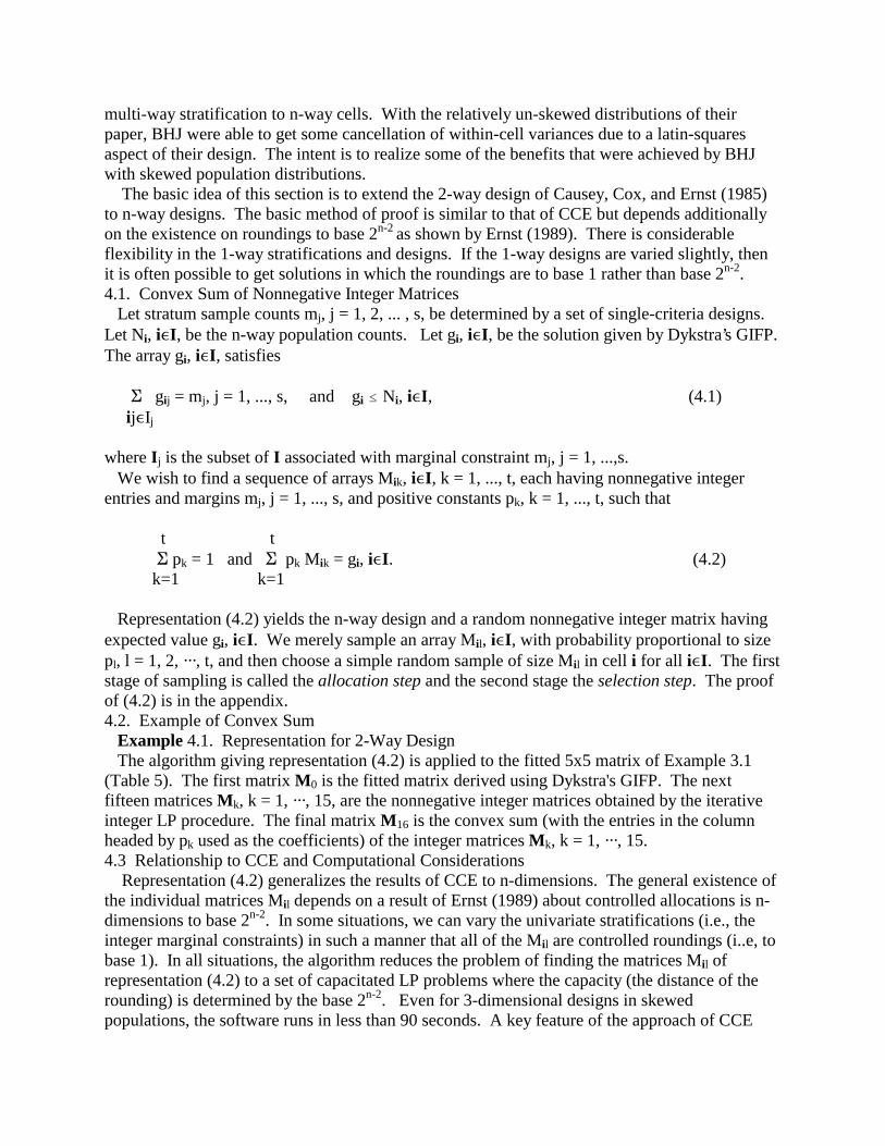
sample were drawn using conventional stratified sampling, then each variable would satisfy a priori specified constraints on their cvs. This would mean that integer marginal constraints of the form mi = Ei,j n(i,j,k) would need to be satisfied. Although we will not be using simple stratified random sampling in the final design, this additional restriction may better allow the final cvs (under the more complicated design) to also approximately satisfy various univariate restraints. Alternatively, we could use a design where ni = n Ni/N where n is the total sample size and Ni/N is the population proportion in cell i. This type of design will generally yield fractional sample sizes in the margins and not, without further restrictions, satisfy univariate cv restraints in moderately skewed population distributions. The advantage of the design of the form ni = n Ni/N is that it is straightforward. The advantage of the method of this paper is that we can take designs in which integer marginal constraints are allowed. The iterative fitting method gives a method of determining individual cell allocations ni when integer marginal constraints are given. The method assures that individual cell values ni are less than the corresponding population proportions Ni/N which cannot be done with classical iterative proportional fitting. The methods of sections 4 and 5 in which a probabilistic structure is given for multi-way sampling and estimation hold for arbitrary ni whether they are given as n Ni/N, by the method of section 3, or some other method. 3. GENERALIZED ITERATIVE PROPORTIONAL FITTING To allocate samples satisfying n single-criteria stratifications to n-way population cells, we use Dykstra’s (1985a,b, 1987, also Winkler 1990) Generalized Iterative Fitting Procedure (GIFP). The initial array is the n-way array of population proportions and the marginal values are the sample allocations to the n sets of single-criteria strata. Deviations of sample proportions from population proportions are minimized on the average (except for rounding) by the systematic fit provided by the Kullback-Leibler measure. If only linear marginal constraints need be satisfied, Dykstra’s GIFP provides answers identical to those provided by classical IPF. Because Dykstra’s GIFP allows convex constraints, we bound sample allocations to n-way cells to be less than their population values. Whereas BHJ required that their 2-way populations have proportions that are products of 1-way population proportions (i.e., independent), we allow fitting to satisfy general interaction restraints in n-way tables (e.g., Bishop, Fienberg, and Holland 1975). Example 3.1. Breakdown of Classical IPF in Sampling Problem Using ordinary IPF with initial matrix N (Table 2) and fixed marginal constraints yields matrix A (Table 3). The entry in cell (1,1) exceeds the population value of 2 units. Applying Dykstra's GIFP with cell (1,1) constrained to be less than or equal to two yields matrix B (Table 4). Winkler (1990) provides another example in which two cells in the matrix obtained by ordinary IPF exceed populations values. After fitting with Dykstra’s GIFP with the two cells restrained to be less than the population value, one of the two fitted cells is less than its upper bound. This demonstrates that Dykstra’s GIFP is a generalization of ordinary IPF even for the simple types of n-way allocations of this paper. The obvious extension of ordinary IPF is to fix the values in the cells that exceed population bounds to be equal to the population bound. The obvious extension will not yield the correct fitted solution. 4. N-WAY DESIGN In the previous section, we addressed the issue of n-way stratification in a manner that generalizes that of BHJ. In this section, we provide a method for allocating the sample of the

multi-way stratification to n-way cells. With the relatively un-skewed distributions of their paper, BHJ were able to get some cancellation of within-cell variances due to a latin-squares aspect of their design. The intent is to realize some of the benefits that were achieved by BHJ with skewed population distributions. The basic idea of this section is to extend the 2-way design of Causey, Cox, and Ernst (1985) to n-way designs. The basic method of proof is similar to that of CCE but depends additionally on the existence on roundings to base 2n-2 as shown by Ernst (1989). There is considerable flexibility in the 1-way stratifications and designs. If the 1-way designs are varied slightly, then it is often possible to get solutions in which the roundings are to base 1 rather than base 2n-2. 4.1. Convex Sum of Nonnegative Integer Matrices Let stratum sample counts mj, j = 1, 2, ... , s, be determined by a set of single-criteria designs. Let Ni, i,I, be the n-way population counts. Let gi, i,I, be the solution given by Dykstra’s GIFP. The array gi, i,I, satisfies E gij = mj, j = 1, ..., s, and gi # Ni, i,I, (4.1) ij,Ij where Ij is the subset of I associated with marginal constraint mj, j = 1, ...,s. We wish to find a sequence of arrays Mik, i,I, k = 1, ..., t, each having nonnegative integer entries and margins mj, j = 1, ..., s, and positive constants pk, k = 1, ..., t, such that t t E pk = 1 and E pk Mik = gi, i,I. (4.2) k=1 k=1 Representation (4.2) yields the n-way design and a random nonnegative integer matrix having expected value gi, i,I. We merely sample an array Mil, i,I, with probability proportional to size pl, l = 1, 2, ···, t, and then choose a simple random sample of size Mil in cell i for all i,I. The first stage of sampling is called the allocation step and the second stage the selection step. The proof of (4.2) is in the appendix. 4.2. Example of Convex Sum Example 4.1. Representation for 2-Way Design The algorithm giving representation (4.2) is applied to the fitted 5x5 matrix of Example 3.1 (Table 5). The first matrix M0 is the fitted matrix derived using Dykstra's GIFP. The next fifteen matrices Mk, k = 1, ···, 15, are the nonnegative integer matrices obtained by the iterative integer LP procedure. The final matrix M16 is the convex sum (with the entries in the column headed by pk used as the coefficients) of the integer matrices Mk, k = 1, ···, 15. 4.3 Relationship to CCE and Computational Considerations Representation (4.2) generalizes the results of CCE to n-dimensions. The general existence of the individual matrices Mil depends on a result of Ernst (1989) about controlled allocations is n-dimensions to base 2n-2. In some situations, we can vary the univariate stratifications (i.e., the integer marginal constraints) in such a manner that all of the Mil are controlled roundings (i..e, to base 1). In all situations, the algorithm reduces the problem of finding the matrices Mil of representation (4.2) to a set of capacitated LP problems where the capacity (the distance of the rounding) is determined by the base 2n-2. Even for 3-dimensional designs in skewed populations, the software runs in less than 90 seconds. A key feature of the approach of CCE

and of this paper is that the algorithm only finds a very small proportion of all individual matrices Mil. Rather than find all of the matrices M that are controlled roundings or controlled allocations, the algorithm finds a very small number that yield representation (4.2). 5. ESTIMATION METHODOLOGY A key facet of the work in this paper is the ability to estimate variances. In the framework of this paper, it is possible to apply a general result of Rao (1975). Alternatives such as bootstrap (e.g., Winkler 1986) can also be used for the n-way designs. CCE did not provide a method of estimating variances. For the 2-way situation, the variance-estimation method of BHJ can be shown to yield very similar results to the estimation methods of this paper. In certain situations, there will be only one unit allocated to an n-way cell. In those situations, within-cell variances can be approximated by collapsing as it is in single-criteria (i.e., univariate) sampling. 5.1. Estimation of the Population Total and Its Variance Let Y be a population total and let Yi be the value for cell i. Let Yi

^ be any unbiased estimator of Yi, i,I. Let Mi

~, i,I, be the random nonnegative integer matrix that takes value Mij, i,I, with probability proportional to size pj (see formula 4.2). Let E(1) denote allocation step expectation and E(2) selection step expectation. Note that E(1)(Mi

~) = gi, i,I. Given a fixed realization of matrix Mi

~ selection step samples are independent. For cell i, let Fi² be the variance of the population mean and let Fi

^² be an estimator such that E(2)(Fi^²) = Fi². In the selection step, any

unbiased estimate of Yi can be used. For the empirical examples of sections 5.2, 5.3, and 5.4 we use Yi

^ = (Ni / Mi~) Ej yij · 1ij,

where yij is the quantitative value assigned to unit ij in cell i and 1ij is the indicator that unit ij is sampled. THEOREM. Let gi, i,I, be the array obtained using Dykstra's GIFP. Let pj, j = 1, ..., t, be nonnegative constants and Mij, i,I, j = 1, ..., t, be nonnegative integer matrices such that t t E pj = 1 and E pj Mij = gi, i,I. j=1 j=1 Let Mi

~, i,I, be the random matrix of sample allocations. An unbiased estimator of the population total is T^ = ∑ (Mi

~ / gi) · Yi^. (5.1)

i,I An unbiased estimator of its variance is v^ = ∑ (Mi

~/gi - 1)²·Yi^² +

i,I

∑ (Mi~/gi - 1)·(Mj

~/gj - 1)·Yi^·Yj

^ + (5.2) i≠j,I ∑ (2·Mi

~/gi - 1)·Ni·(Ni - Mi~)·Fi

^²/Mi. i,I The summations are over gi > 0. Cells i,I for which gi = 0 have no n-way population members. The proofs of (5.1) and (5.2) are in the appendix. 5.2. Example of Variance Estimation for a 2-Way Design Example 5.1 shows that, for fixed size samples, estimators under the multi-way design can have lower total variation for two variables than total variation under judiciously chosen single-criteria designs. Example 5.1. Estimation Under a Two-Way Design We use the database of Example 4.1. Each record contains volumetric data representing the sales of distillate fuel oil in residential and nonresidential end-use sectors. A generalized version of the Dalenius-Hodges method (Cochran, 1977, pp. 127-129, Winkler 2000) is used for single-criteria stratification. The single-criteria designs are highly non-proportional. The magnitudes of the nonzero values range from 72,000 to 1 for the first variable and from 85,000 to 1 for the second. The second variable only takes nonzero values for 60 percent of the records. To reduce cvs, each single-criteria design allocates the same 13 records with certainty. The remaining 1251 records are stratified into two different sets of five strata having a total sample allocation of 37. Each design has strata sample allocations of 6, 6, 7, 8, and 10. The cvs are 0.044 and 0.028, respectively. The first 13 records are also allocated with certainty under the 2-way design. Single-criteria strata boundaries apportion the remaining 1251 records into a 5x5 array. The results of the two single-criteria stratifications and the corresponding 2-way design are compared with two optimal single-criteria designs (Table 6). Given the sample size of 50, the optimal designs yield minimal cvs for exactly one variable. To do this, the optimal designs allocate less than 13 records with certainty. Sufficiently many noncertainty strata are created so that only two sample elements are allocated in each. The first set of four cvs is for optimal univariate designs in which the stratifying variable agrees with one of the variables being estimated. Diagonal elements are low (0.012 and 0.009). Off-diagonal elements are dramatically higher (0.334 and 0.407) because the stratifying variables are not highly correlated with the variables for which the cvs are computed. Regression using the two variables yields an R-square value less than 0.2. If, however, we apply standard contingency table techniques (Bishop, Fienberg, and Holland, 1975) to the underlying population matrix N (Table 2), we reject independence at the 95 percent level of confidence. The second set of numbers is for single-criteria designs used in creating the 2-way stratification. Diagonal elements (0.044 and 0.028) are higher than the diagonal elements in the first matrix. Off-diagonal entries, 0.289 and 0.282, are lower. The final set consists of the cvs 0.104 and 0.041 for the 2-way design. They are also higher than the diagonal entries in the first matrix and approximately twice as high the diagonal entries in the second matrix. They are substantially lower than the highest of the off-diagonal entries for the respective variables (0.334 and 0.407). Using the stratification given by the first row of the first matrix, we have total variation 0.334 while the n-way design yields total variation 0.112. Ignoring the finite

population correction (fpc), sample size must increase by a factor greater than 6 to equal the total variation and cvs of the n-way case. Five hundred independent samples were drawn to evaluate the empirical performance of the estimators based on the 2-way design. The relative empirical biases were 0.008 and 0.000, and the empirical cvs were 0.100 and 0.036, respectively. The biases of 0.04 and 0.05 in the estimated cvs follow because we must approximate within-cell variances of cells having sample allocations of one. The approximation involved substituting the minimum of the within-row and within-column variances for each such cell. The approximation generally overestimates the within-cell variance. 5.3. Three-Way Variance Example This example involves a 3-way design using three single-criteria stratifications. The database and procedures are similar to those in Example 5.1. The single-criteria designs had the same 15 units allocated with certainty and a remaining 50 units allocated in 4, 4, and 2 strata that were determined by three different measures of size, respectively. Thus, the 3-way design array is 4x4x2. Total variation ranged from 0.466 (the best in the case of standard single-criteria stratification techniques) to 0.115 (multi-way) (Table 7). Ignoring the fpc, we would have to increase the sample size by a factor greater than 16 to equal the total variation and cvs given for the multi-way design. Based on 200 independent samples, the empirical biases of the multi-way estimators of the three variables were -0.004, 0.000, and -0.004, respectively. The empirical cvs were 0.070, 0.056, and 0.73, and the biases of the estimates of the cvs were 0.001, 0.001, and -0.002, respectively. 5.4. Components of Variance For the 3-way design example of section 5.3, the within-cell variance component (last summation in equation (5.2)) contributes an average of 67, 83, and 86 percent to the total variance for variables 1, 2, and 3, respectively (Table 8). The average is based on fifteen samples. The extremes are 41 and 100 percent, 27 and 100 percent, and 45 and 100 percent for variables 1, 2, and 3, respectively. 6. DISCUSSION The main strategy of multi-way stratification is in two steps. First, develop single-criteria designs that are not much worse than optimal single-criteria designs. Second, assure that the single-criteria designs can be allocated to n-way cells in a manner that is most consistent with the population proportions in those cells. The method of BHJ, SS, and this paper all provide a representation of the form (4.2) that, in turn, allows the association of a probabilistic model with a design ni. 6.1. Problem Posed in Neyman Paper Neyman (1934, p. 579) observed that stratification can increase the precision of an estimator. Bowley (Neyman 1934, p. 608), in his discussion, noted that the stratification and selection of units for one purpose is not necessarily the best for other purposes. This paper presents n-way designs that allow moderate regulation of the precision of estimators of totals for sets of non-correlated variables. 6.2. Relationship to the Design of BHJ For some populations and pairs of designs BHJ could show (1960, section 9) that, within a very small correction factor, variances under the 2-way design for the estimators of totals were less than or equal the variances under the single-criteria designs. If we use the convex

representation of BHJ for such a situation, then estimator (5.1) gives the same total as estimator (10) of BHJ (when appropriately modified for totals instead of means). The probability structures of the 2-way designs agree and estimator (5.2) gives the same theoretical variance as the BHJ variance (1960, equation 12) (also when properly modified for totals). Generally, the probabilistic structure associated with the estimators depends on the convex sum. The convex sum of BHJ contains all possible roundings of the sample allocation matrix. Representation (4.2) contains a subset of all possible roundings and is not unique. 6.3. Relationship to the work of Sitter and Skinner Sitter and Skinner (1994) extend ideas from Rao and Nigam (1990, 1992). In this section, we will indicate a more plausible reason why their method improved over that of BHJ for the type of simulated data that they considered. We will also demonstrate why the methods of this paper are more general and computationally more tractable in large situations. SS explicitly wanted to restrict their two-way designs to the form: ∑s∈Sn nij(s) p(s) = nPij for i = 1, …, R and j = 1, …, C. (6.1) Here Pij = Nij/N, n is the sample size, and Sn are designs having sample size n. Representation (6.1) corresponds to the representation (4.2) of the Theorem of this paper. A key difference and difficulty is that SS needed to know all of the integer arrays nij(s) prior to running their LP algorithms. The integer arrays nij(s) are part of the restraints of the LP problem. As SS indicated, when there are more constraints, equation (6.1) is difficult to solve using the LP method of their paper but should be easier to solve using a method similar to the method of CCE. The method of this paper solves the equivalent situation for higher dimensional situations and for populations of variables that are reasonably highly skewed. It should be far faster than the LP method of SS. The method of CCE was not extended beyond two dimensions. It is not clear how individuals could find all integer arrays nij(s) corresponding to a design ni in three or more dimensions. If one does not have all of the integer arrays nij(s) prior to solving (6.1) using the LP method of SS, then one cannot generally solve (6.1). Thus, the challenges go beyond the straightforward computational difficulties pointed out by SS. SS explicitly minimized a loss function of the form: w(s) = ∑i (ni.(s) – nPi.)

2 – ∑j (n.j(s) – nP.j)2. (6.2)

As SS indicated, there are designs for which the minimal solution of (6.2) is zero. The designs of this paper (even in higher dimension) yield minimal solution of zero for equation (6.2). SS (section 2.3) indicated how their LP method could be extended to higher dimensions using a squared-error loss function for which different variables could be weighted by various factors. Their method does not generally yield a minimal solution of zero. SS indicated that their method is better at controlling the covariances Cov(nij, ni’j’ ) which directly affect the between-cell variance. A more plausible explanation, as shown in this paper, is that their method was better at controlling the allocated proportions nij to be close to nPij than the method of BHJ. The designs of this paper had restraints in which the univariate stratifications all had integer allocations that were greater than 1. As an approximation for the estimate of the within-cell variance Si

2, we can use the minimum of the appropriate 1-dimensional variances. If i = (i,j), then we can use the minimum of the estimates from the sample values associated with row i or

with column j. SS assume that the variance Si2 are constant across cells i. They also assume

that Si2 can be estimated by the values in a cell having allocated sample greater than 1. With

moderately skewed population distributions, their assumptions would yield inappropriate estimates of Si

2. Their within-cell variance estimates could be strongly biased upwards or downwards. The methods of this paper easily extend to three or more dimensions. 7. SUMMARY This paper presents a methodology for using two or more single-criteria stratifications to produce a multi-way stratification of the population. If each single-criteria design allows control over the precision of estimators of totals for one variable, then multi-way stratification, with no increase in sample size, can yield estimators having only moderate loss of precision for all variables. 1/ This paper reports the results of research and analysis undertaken by Census Bureau staff. It has undergone a Census Bureau review more limited in scope than that given to official Census Bureau publications. This report is released to inform interested parties of research and to encourage discussion.

REFERENCES Bishop, Y., Fienberg, S., and Holland, P. (1975), Discrete Multivariate Analysis, MIT Press, Cambridge, MA. Bryant, E., Hartley, H., and Jessen, R. (1960), "Design and Estimation in Two-Way Stratification," Journal of the American Statistical Association, 55, 105-124. Causey, B., Cox, L., and Ernst, L. (1985), "Applications of Transportation Theory to Statistical Problems," Journal of the American Statistical Association, 80, 903-909. Cochran, W. (1977), Sampling Techniques, Third Edition, J. Wiley, New York. Cox, L. and Ernst, L. (1982), "Controlled Rounding," Informatics, 20, 423-432. Dantzig, G. (1963), Linear Programming and Its Extensions, Princeton University Press, Princeton, N.J. Dykstra, R. (1985a), "An Iterative Procedure for Obtaining I-Projections onto the Intersection of Convex Sets," Annals of Probability, 13, 975-984. Dykstra, R. (1985b), "Computational Aspects of I-Projections," Journal of Statistical Computation and Simulation., 21 265-274. Dykstra, R. and Wollan, P. (1987), "Finding I-Projections Subject to a Finite Set of Linear Inequality Constraints," Applied Statistics, 36 377-383. Ernst, L. R. (1989), "Further Applications of Linear Programming to Sampling Problems," American Statistical Association, Proceedings of the Section on Survey Research Methods, 625-631. Gass, S. (1986), Linear Programming, Fifth Edition, McGraw-Hill, N.Y. Green, J. (2000), “Mathematical Programming for Sample Design and Allocation Problems,” American Statistical Association, Proceedings of the Section on Survey Research Methods, 688-692. Neyman, J. (1934), "On the Two Different Aspects of the Representative Method: The Method of Stratified Sampling and the Method of Purposive Selection," Journal of the Royal Statistical Society B, 97, 558-606. Rao, J. N. K. (1975), "Unbiased Variance Estimation for Multistage Designs," Sankhya, Series

C, 37 133-139. Rao, J. N. K. and A. K. Nigam (1990), “Optimal Controlled Sampling Designs,” Biometrika, 77, 907-814. Rao, J. N. K. and A. K. Nigam (1992), “Optimal Controlled Sampling: a Unified Approach,” International Statistical Review, 60, 89-98. Sitter, R. R. and C. J. Skinner (1994), “Multi-way Stratification by Linear Programming,” Survey Methodology, 20, 65-73. Winkler, W. E. (1986), “Multi-Purpose Survey Sampling,” American Statistical Association, Proceedings of the Section on Survey Research Methods, 614-619. Winkler, W. E. (1987), “An Application of Multi-Purpose Survey Sampling,” American Statistical Association, Proceedings of the Section on Survey Research Methods, 200-204. Winkler, W. E. (1990), “On Dykstra’s Iterative Fitting Procedure,” Annals of Probability, 18, 1410-1415. Winkler, W. E. (1998), “Strata Boundary Determination,” U.S. Bureau of the Census, Statistical Research Division Report rr98/03 (http://www.census.gov/srd/www/byyear.html).

APPENDIX To prepare for the proof of equation (4.2), we need more formal definitions and notation. We consider arrays in n dimensions. Let Ri, i,I, be a array of nonnegative integers, Ai, i,I, be an array of nonnegative reals, and mj, j = 1, ...,s, be a set of positive integer marginal restraints. We say that a nonnegative integer array Mi, i,I, is a controlled allocation with restraint array Ri, i,I, for array Ai, i,I, if A i, i,I, and Mi, i,I, each have margins mj, j = 1, ..., s, and |Ai - Mi| < Ri if A i is not an integer and Ai = Mi if Ai is an integer or zero. Array Ri, i,I, controls how far the allocated array Mi, i,I, can deviate from the original array Ai, i,I. We observe that Ri must necessarily take positive values if Ai is not an integer. Ri can take any nonnegative integer value if Ai is an integer. We will say that nonnegative real array Ai, i,I, has a controlled allocation if we can find nonnegative integer arrays Mi, i,I, and Ri, i,I, such that Mi, i,I, is a controlled allocation with restraint array Ri, i,I, for Ai, i,I. If the restraint array Ri, i,I, consists of zeros and ones and has the property that if Ai is an integer then Ri is zero, we say that Mi, i,I, is a controlled rounding of Ai, i,I. See Ernst (1989) for more information. Restraint arrays need not be unique. For convenience, we will generally only consider the smallest restraint array controlling the allocation of an arbitrary array Ai, i,I, to a nonnegative integer array Mi, i,I. By smallest, we mean that no other nonnegative integer array having entries that are less than or equal the corresponding entries in Ri, i,I, and having one entry that is strictly less can serve as the restraint array. The smallest restraint array is unique. The allocated array Mi, i,I, is generally not unique even if the restraint array is the smallest. In the proof of (4.2) the restraint matrix Ri, i,I, will be fixed for all controlled allocations. The restraint matrix will not be referred to because the proof does not depend on its explicit form.

Proof of (4.2). We define sequence of arrays Aik, i,I, k = 1, ..., t, Mik, i,I, k = 1, ..., t, and positive constants pk, k = 1, ..., t, inductively. For k = 1, let Ai1 = gi, i,I, and let Mi1, i,I, be any controlled allocation of Ai1, i,I. Define Bi1, i,I as follows: if Ai1 - Mi1 > 0 then Bi1 is the smallest integer greater than Ai1, if Mi1 - Ai1 > 0 then Bi1 is the largest integer smaller than Ai1, and if Mi1 = Ai1 then Bi1 = 0. Let I1 = {i,I: Ai1 ≠ Mi1}, e1 = max |(Ai1 - Mi1)/(Mi1 - Bi1)|, i,I1 p1 = (1 - e1), and Ai2 = Mi1 + (Ai1 - Mi1) / e1, i,I. For k > 1, let Mik, i,I, be any controlled allocation of Aik, i,I. Define Bik, i,I as follows: if Aik - Mik > 0 then Bik is the smallest integer greater than Aik, if Mik - Aik > 0 then Bik is the largest integer smaller than Aik, and if Mik = Aik then Bik = 0. Let Ik = {i,I: Aik ≠ Mik}, ek / max |(Aik - Mik)/(Mik - Bik)|, (A.1) i,Ik k-1 pk = (1 - E pj ) (1 - ek), (A.2) j=1 Aik+1 = Mik + (Aik - Mik) / ek, i,I. (A.3) Observe that Aik $ 0 for i,I and all k. If Aik becomes an integer for some k, then it remains an integer for subsequent values of k. At each step k, one additional cell of Aik+1 (the one associated with the normalized maximum deviation ek) is set to an integer value. As I is finite, by (A.1), there exists a smallest integer t such that et = 0 if and only if controlled allocations Mik exist for k = 1, 2, ···, t. t We now show that E pk Mik = Ai, i,I. k=1 Solving (A.3) for Mik and multiplying by pk, we obtain pk Mik = pk (Aik - ek Aik+1)/(1 - ek) which together with (A.1) yields p1 Mi1 = Ai1 + (p1 - 1)/ Ai2 and, for 2 # k # t,

k-1 k pk Mik = (1 - E pj) Aik + (E pj - 1)) Aik+1. j=1 j=1 Consequently, t-1 t-1 E pk Mik = Ai1 + ( E pj - 1) Ait k=1 j=1 = Ai1 + (-pt) Ait, i,I, which, in turn, yields the desired result. ��� Proof of (5.1) and (5.2). We have that E(T^) = E(1)E(2)( E (Mi

~ / gi) · Yi^)

i,I = E(1)( E (Mi

~ / gi) · Yi) i,I = E Yi = Y, i,I where Y is the true population total. We observe that E(1)(M i

~/gi) = 1 and that, conditional on the allocation step, sampling under the selection step is independent across cells. Now, T^ = E (Mi

~ / gi) · Yi^

i,I = E (Mi

~/gi)·Yi + E (Mi~/gi)·(Yi

^-Yi) / A1 + A2. i,I i,I As in BHJ (1960, pp. 113-114), it is straightforward to show that A1 and A2 are uncorrelated under the selection step and that f(Y) / E (Mi

~/gi-1)²·Yi² + i,I

E (Mi~/gi-1)·(Mj

~/gj-1)·Yi·Yj i≠j,I is an unbiased estimator of Var(A1). Consequently, we may apply Theorem of Rao (1975) to obtain (5.2). Specifically, ais, bis, and dijs in Rao's formulas are replaced by Mi

~/gi, (Mi~/gi - 1)², and (Mi

~/gi - 1)·(Mj~/gj - 1),

respectively. �

Table 1. Examples of Matrices Illustrating Controlled Allocations Matrix A 1.1 0.7 1.0 0.5 0.7 | 4 1.1 1.5 0.0 0.1 0.3 | 3 0.0 0.5 0.4 0.1 0.0 | 1 0.2 0.1 0.6 0.1 0.0 | 1 0.6 0.2 0.0 0.2 0.0 | 1 ----------------------------- 3 3 2 1 1 | 10 Matrix B 2.0 0.0 1.0 0.0 1.0 | 4 0.0 3.0 0.0 0.0 0.0 | 3 0.0 0.0 1.0 0.0 0.0 | 1 0.0 0.0 0.0 1.0 0.0 | 1 1.0 0.0 0.0 0.0 0.0 | 1 ----------------------------- 3 3 2 1 1 | 10 Matrix C 2.0 0.0 1.0 0.0 1.0 | 4 1.0 2.0 0.0 0.0 0.0 | 3 0.0 1.0 0.0 0.0 0.0 | 1 0.0 0.0 1.0 0.0 0.0 | 1 0.0 0.0 0.0 1.0 0.0 | 1 ----------------------------- 3 3 2 1 1 | 10

Table 2. Population Counts N Induced by Two Single-Criteria Stratifications 1/ Var 1 Variable 2 Strata Strata 1 2 3 4 5 Total 1 2 7 4 1 11 | 25 2 3 5 7 17 31 | 63 3 0 10 16 47 85 | 158 4 2 3 10 78 257 | 350 5 3 5 29 67 551 | 655 ----------------------------- 10 30 66 210 935 |1251 1/ The quantitative measures of size associated with the variables, by strata, are: Variable 1- 1 : 20589-8116, 2 : 8115-3501, 3 : 3500-1501, 4 : 1500-501, and 5 : 500-0; and Variable 2- 1 : 16423-5195, 2 : 5194-2260, 3 : 2259-648, 4 : 647-152, and 5 : 150-0.

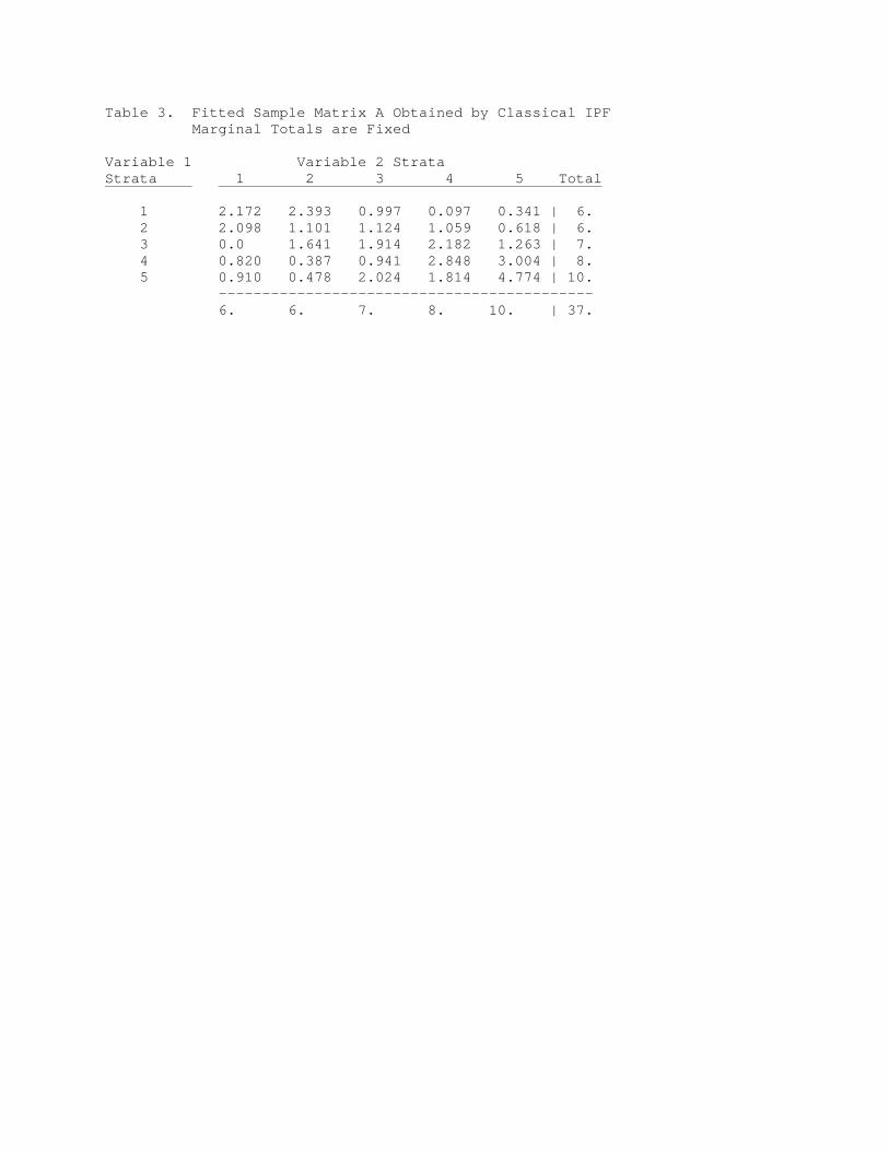
Table 3. Fitted Sample Matrix A Obtained by Classical IPF Marginal Totals are Fixed Variable 1 Variable 2 Strata Strata 1 2 3 4 5 Total 1 2.172 2.393 0.997 0.097 0.341 | 6. 2 2.098 1.101 1.124 1.059 0.618 | 6. 3 0.0 1.641 1.914 2.182 1.263 | 7. 4 0.820 0.387 0.941 2.848 3.004 | 8. 5 0.910 0.478 2.024 1.814 4.774 | 10. ------------------------------------------- 6. 6. 7. 8. 10. | 37.

Table 4. Fitted Sample Matrix B Obtained by Dykstra’s GIFP Marginal Totals are Fixed Variable 1 Variable 2 Strata Strata 1 2 3 4 5 Total 1 2.000 2.483 1.052 0.103 0.362 | 6. 2 2.182 1.061 1.101 1.046 0.610 | 6. 3 0.0 1.614 1.914 2.200 1.272 | 7. 4 0.860 0.377 0.930 2.840 2.993 | 8. 5 0.958 0.465 2.003 1.811 4.763 | 10. ------------------------------------------- 6. 6. 7. 8. 10. | 37.

Table 5. Example of Iterative Integer LP Procedure Cell of Matrix Mk ------------------------------------------------------ k pk (1,1) (1,2) (1,3) (1,4) (1,5) (2,1) (2,2) (2,3) ----------------------------------------------------------------- 0 0.000 2.000 2.483 1.052 0.103 0.362 2.182 1.061 1.101 1 0.140 2.000 3.000 1.000 0.000 0.000 3.000 1.000 1.000 2 0.042 2.000 3.000 1.000 0.000 0.000 3.000 1.000 1.000 3 0.007 2.000 2.000 1.000 0.000 1.000 2.000 2.000 1.000 4 0.054 2.000 3.000 1.000 0.000 0.000 2.000 2.000 1.000 5 0.029 2.000 3.000 1.000 0.000 0.000 2.000 1.000 2.000 6 0.114 2.000 3.000 1.000 0.000 0.000 2.000 1.000 1.000 7 0.104 2.000 3.000 1.000 0.000 0.000 2.000 1.000 1.000 8 0.017 2.000 2.000 2.000 0.000 0.000 2.000 1.000 1.000 9 0.035 2.000 2.000 2.000 0.000 0.000 2.000 1.000 1.000 10 0.003 2.000 2.000 1.000 0.000 1.000 2.000 1.000 1.000 11 0.032 2.000 2.000 1.000 0.000 1.000 2.000 1.000 2.000 12 0.043 2.000 2.000 1.000 0.000 1.000 2.000 1.000 1.000 13 0.237 2.000 2.000 1.000 0.000 1.000 2.000 1.000 1.000 14 0.040 2.000 2.000 1.000 0.000 1.000 2.000 1.000 2.000 15 0.103 2.000 2.000 1.000 1.000 0.000 2.000 1.000 1.000 16 1.000 2.000 2.483 1.052 0.103 0.362 2.182 1.061 1.101 Cell of Matrix Mk ------------------------------------------------------------- k (2,4) (2,5) (3,1) (3,2) (3,3) (3,4) (3,5) (4,1) (4,2) ------------------------------------------------------------------ 0 1.046 0.610 0.000 1.614 1.914 2.200 1.272 0.860 0.377 1 1.000 0.000 0.000 1.000 2.000 2.000 2.000 0.000 1.000 2 1.000 0.000 0.000 1.000 2.000 2.000 2.000 1.000 0.000 3 1.000 0.000 0.000 1.000 2.000 2.000 2.000 1.000 1.000 4 1.000 0.000 0.000 1.000 2.000 2.000 2.000 1.000 0.000 5 1.000 0.000 0.000 1.000 1.000 3.000 2.000 1.000 1.000 6 1.000 1.000 0.000 1.000 2.000 3.000 1.000 1.000 1.000 7 1.000 1.000 0.000 2.000 2.000 2.000 1.000 1.000 0.000 8 1.000 1.000 0.000 2.000 1.000 3.000 1.000 1.000 1.000 9 1.000 1.000 0.000 2.000 2.000 2.000 1.000 1.000 1.000 10 2.000 0.000 0.000 2.000 2.000 2.000 1.000 1.000 1.000 11 1.000 0.000 0.000 2.000 2.000 2.000 1.000 1.000 1.000 12 2.000 0.000 0.000 2.000 2.000 2.000 1.000 1.000 0.000 13 1.000 1.000 0.000 2.000 2.000 2.000 1.000 1.000 0.000 14 1.000 0.000 0.000 2.000 1.000 3.000 1.000 1.000 0.000 15 1.000 1.000 0.000 2.000 2.000 2.000 1.000 1.000 0.000 16 1.046 0.610 0.000 1.614 1.914 2.200 1.272 0.860 0.377

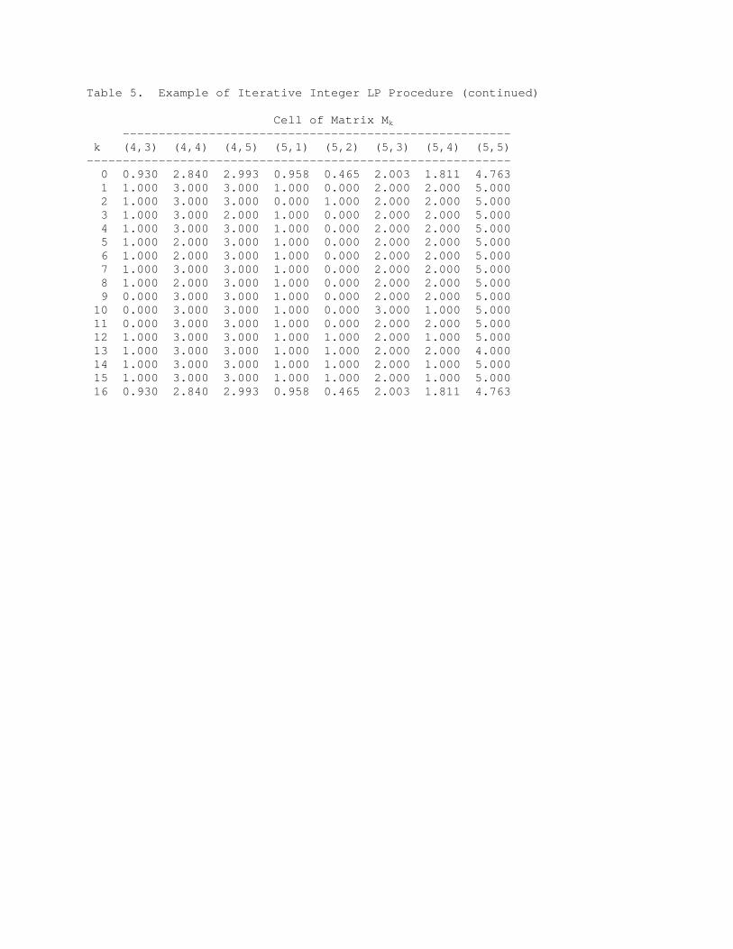
Table 5. Example of Iterative Integer LP Procedure (continued) Cell of Matrix Mk ------------------------------------------------------ k (4,3) (4,4) (4,5) (5,1) (5,2) (5,3) (5,4) (5,5) ----------------------------------------------------------- 0 0.930 2.840 2.993 0.958 0.465 2.003 1.811 4.763 1 1.000 3.000 3.000 1.000 0.000 2.000 2.000 5.000 2 1.000 3.000 3.000 0.000 1.000 2.000 2.000 5.000 3 1.000 3.000 2.000 1.000 0.000 2.000 2.000 5.000 4 1.000 3.000 3.000 1.000 0.000 2.000 2.000 5.000 5 1.000 2.000 3.000 1.000 0.000 2.000 2.000 5.000 6 1.000 2.000 3.000 1.000 0.000 2.000 2.000 5.000 7 1.000 3.000 3.000 1.000 0.000 2.000 2.000 5.000 8 1.000 2.000 3.000 1.000 0.000 2.000 2.000 5.000 9 0.000 3.000 3.000 1.000 0.000 2.000 2.000 5.000 10 0.000 3.000 3.000 1.000 0.000 3.000 1.000 5.000 11 0.000 3.000 3.000 1.000 0.000 2.000 2.000 5.000 12 1.000 3.000 3.000 1.000 1.000 2.000 1.000 5.000 13 1.000 3.000 3.000 1.000 1.000 2.000 2.000 4.000 14 1.000 3.000 3.000 1.000 1.000 2.000 1.000 5.000 15 1.000 3.000 3.000 1.000 1.000 2.000 1.000 5.000 16 0.930 2.840 2.993 0.958 0.465 2.003 1.811 4.763

Table 6. CVs for Single-Criteria Designs and 2-Way Design 1/ CVs | Total ---------------|Variation Var 1 | Var 2 | 2/ ================================================== Optimal Single-Criteria Stratifying Var 1 .012 .334 .334 Stratifying Var 2 .407 .009 .407 Single-Criteria Designs for Multi-Way Design Stratifying Var 1 .044 .289 .292 Stratifying Var 2 .282 .028 .283 Multi-Way Design .104 .041 .112 -------------------------------------------------- 1/ Each of the second set of single-criteria designs and the 2-way design allocate the same 13 population members with certainty and 37 randomly to the strata containing the remaining 1251 population members. 2/ Square root of the sum of squares of two CV columns.

Table 7. CVs for Single-Criteria Designs and 3-Way Design 1/ CVs | Total -----------------------|Variation Var 1 | Var 2 | Var 3 | 2/ ========================================================== Optimal Single-Criteria Stratifying Var 1 .001 .490 .372 .615 Stratifying Var 2 .306 .001 .351 .466 Stratifying Var 3 .604 .884 .001 1.071 Single-Criteria Designs for Multi-Way Design Stratifying Var 1 .047 .291 .221 .368 Stratifying Var 2 .178 .043 .194 .267 Stratifying Var 3 .207 .272 .065 .349 Multi-Way Design .071 .055 .071 .115 ---------------------------------------------------------- 1/ Each of the second set of single-criteria designs and the 3-way design allocate the same 15 population members with certainty and 50 randomly to the strata containing the remaining population members. 2/ Square root of the sum of squares of three cv columns.

Table 8. Components of Variance for 3-Way Design Example Fifteen Samples | Estimated | CV | Within-Cell | Total 1/ | | Variance Proportion | Variable | Variable | Variable | 1 | 2 | 3 | 1 | 2 | 3 | 1 | 2 | 3 ------------------------------------------------------------------- 1,423 1,195 1,684 .101 .056 .083 .48 .99 .75 1,384 1,297 1,576 .059 .056 .042 1.00 .92 .89 1,337 1,269 1,450 .083 .050 .021 .54 .78 .80 1,278 1,246 1,469 .060 .045 .035 .82 .81 .97 1,387 1,246 1,696 .048 .059 .090 .60 .96 1.00 1,345 1,119 1,630 .056 .074 .038 .92 .83 .95 1,211 1,194 1,554 .061 .045 .046 .91 .84 .92 1,460 1,226 1,636 .104 .049 .061 .50 .79 .98 1,355 1,191 1,540 .057 .039 .052 .42 1.00 .72 1,428 1,250 1,843 .100 .069 .098 .41 .98 .99 1,345 1,259 1,845 .071 .087 .083 .51 .71 .99 1,271 1,229 1,808 .063 .075 .089 .76 .62 .86 1,424 1,336 1,550 .047 .067 .043 .95 .27 .82 1,436 1,115 1,637 .085 .029 .054 .49 .98 .45 1,497 1,285 1,833 .051 .066 .095 .81 .97 .88 ------------------------------------------------------------------- AVER 1,372 1,230 1,650 .073 .060 .070 .67 .83 .86 ------------------------------------------------------------------- 1/ True values are 1354, 1254, and 1654.