University of Massachusetts AmherstScholarWorks@UMass Amherst

Wind Energy Center Reports UMass Wind Energy Center

1977

Wind And Solar Residential Heating Systems.Energy And Economics StudyGhazi Darkazalli

John G. McGowan

Follow this and additional works at: https://scholarworks.umass.edu/windenergy_report

Part of the Mechanical Engineering Commons

This Article is brought to you for free and open access by the UMass Wind Energy Center at ScholarWorks@UMass Amherst. It has been accepted forinclusion in Wind Energy Center Reports by an authorized administrator of ScholarWorks@UMass Amherst. For more information, please contactscholarworks@library.umass.edu.

Darkazalli, Ghazi and McGowan, John G., "Wind And Solar Residential Heating Systems. Energy And Economics Study" (1977).Wind Energy Center Reports. 4.Retrieved from https://scholarworks.umass.edu/windenergy_report/4

UNNERSrrY OF MASSACHUSETTS/AMHERST ENERGY ALTERNATIVES PROGRAM

WIND AND SOLAR RESIDENTIAL HEATING SYSTEMS:

ENERGY AND ECONOMICS STUDY

Ghazi Darkaza l l i

and

Jon G. McGowan

UMass Wind Furnace

Energy A1 t e r n a t i ves Program

U n i v e r s i t y o f Massachusetts

Arr~hers t , Mass 01 003

January 1977

Report: WF/TR/77/1

ABSTRACT

Th is work i s p r i m a r i l y concerned w i t h t h e a n a l y t i c a l design of wind

space and water heat ing systems f o r residences. A development o f a d i g i t a l

computer based methodology t o c a l c u l a t e system performance and cos ts i s

presented. I n a d d i t i o n t o wlnd powered systems, so la r , and combined wind

and s o l a r systems are considered i n d e t a i l , The ana lys i s i s based on two

separate computer programs: An energy program t h a t determines system per-

formance as a f u n c t i o n o f subcomponent parameters and a u x i l i a r y energy

requirements, and an economics program t h a t ca l cu la tes present and f u t u r e

(mass produced) cos ts o f the wind and/or s o l a r components and system. Com-

p l e t e d e t a i l s o f a l l p a r t s o f t h e model, which i s intended t o be a general

design t o o l f o r such systems, a r e presented.

The r e s u l t s i nc lude a d e t a i l e d se r ies o f runs based on h o u r l y weather

and s o l a r data f o r a " t y p i c a l " New England s i t e , us ing an "Average"

and "Mociel " (we1 1 i nsu la ted ) res idence model . A1 so, a d d i t i o n a l runs are

presented f o r o the r s i t e s and residences. The performance and economic

r e s u l t s show t h a t wind and/or s o l a r systems are p resen t l y compet i t i ve w i t h

e l e c t r i c based heat ing systems. I t i s a l s o shown t h a t i n t h e f u t u r e such

systems w i l l be compet i t i ve w i t h o i l o r na tu ra l gas hea t i ng systems.

TABLE OF CONTENTS

Page

Abst rac t

Table of Contents

L i s t o f Figures

L i s t o f Tables

I I n t r o d u c t i o n

I1 Descr ip t ion o f t he Overa l l System Conf igurat ion

2.1 Model 1 System

2.2 Model 2 System

2.3 Model 3-A System

2.4 Model 3-B System

2.5 Domestic Hot Water Model

I 1 1 System Components Desc r ip t i on

3.1 The W i ndpower System

3.1 .1 H i s t o r i c a l Background

3.1 .2 W i ndpower - Basic Fundamental s

3.1.3 Power Losses

3.2 The F l at -Pl a t e Col l e c t o r Subsystem

3.2.1 Solar Rad ia t ion - I n p u t

3.2.2 The F l a t -P l a te Col 1 ec to r

3.2.3 The C o l l e c t o r Model

3.2.4 Re f lec t i on Losses

3.2.5 Absorpt ion Losses

3.2.6 Heat Losses from the Absorber P l a t e

3.2.7 Overa l l Col l e c t o r Energy Balance

3.3 Energy Storage

3.3.1 Background

3.3.2 Storage A n a l y t i c a l Model

3.4 The House

3.4.1 Res ident ia l Homes

3.4.2 The General House Model

3.5 The Heat De l i ve ry Model

I V The Computer A n a l y t i c a l Models

4.1 The Main Program

4.2 The Data Sub-program

4.3 The Wind Sub-program

4.4 So lar Sub-program

4.5 The Load Sub-program

4.6 The Heat Exchanger Sub-program

4.7 The Domestic Hot Water (D.H.W.) Subrout ine

V System Performance and A n a l y t i c a l Results

5.1 General Background

5.2 De ta i l ed A n a l y t i c a l Results

5.3 Domesti c Hot Water Heating A n a l y t i c a l Results

5.4 Systems Performance a t Other S i tes

V I he System Economic Model

6.1 Background

6.2 System's I n d i v i d u a l Components Cost Ana lys is

Page

35

6.2.1 Storage Cost, CST

6.2.2 So la r C o l l e c t o r Cost, CC

6.2.3 Windmi l l Cost, CW

a. Tower Cost, CT - b. Rotor Cost, CR

c. Frame and Transmission Costs, CB

d. Generator Cost, CG

6.2.4 Heat D e l i v e r y System Cost, CD

6.3 The Cost o f t h e A u x i l i a r y Heat ing System, CAUX

6.4 Fuel and Conventional Heat ing System Cost, CF

and 'CON

6.4.1 Natura l Gas

6.4.2 O i l Cost

6.4.3 E l e c t r i c i t y Cost

6.5 To ta l and Annual System Cost

V I I Economic Study Resul ts

7.1 I n t r o d u c t i o n

7.2 Economics Computer Ana lys is

7.3 The UMass Model 3-A System Cost

7.4 Other Systems Costs

7.4.1 Fuel Costs

7.4.2 Conventional Systems Costs

7.4.3 Wind and So la r Systenis Costs

7.5 Summary o f Resul ts

7.6 Systems' Costs w i t h Domestic Hot Water Heat ing

Page

1 30

134

139

143

1 48

148

1 48

153

153

Page

VIII Conclusions and Recommendations

8.1 Conclusions

8.2 Recommendations f o r Future Studies

References

Appendix A , Nomenclature

Appendix B, Computer Main Program

Appendix C, Tabulated Sample Resclts

LIST OF FIGURES

2.1 Model 1 No-Storage Wind System

Page

9

2.2 Model 2 Wind System With Storage 11

2.3 Model 3-A So la r and Wind System With One Storage 12

2.4 Model 3-B So la r and Wind System w i t h Two Storage Tanks 14

2.5 Domestic Hot Water System

3.1 Windmi 11 Rotor and V e l o c i t i e s

3.2 Wind V e l o c i t i e s and Forces a t a Blade Element

3.3 The Wind Generator Performance Curves

3.4 Comparison o f t h e A n a l y t i c a l and Theore t i ca l Curves 27 o f t h e Wind Generator (D = 32.5 ft. ) .

3.5 F l a t P l a t e C o l l e c t o r Design

3.6 I l l u s t r a t i o n o f S n e l l ' s Law

3.7 F l a t P l a t e So lar C o l l e c t o r

3.8 Storage Tank and So la r C o l l e c t o r System

3.9 Temperature D i s t r i b u t i o n i n Single-Pass Counter Flow 49 Heat Exchanger

3.1 0 Counter- F l ow Heat Exchanger 50

Computer Program Block Diagram

The Main Program Flow Diagram

Flow Diagram o f t h e Data Sub-program

Wind Sub-program Flow Diagram

So la r Sub-program Block Diagram

Flow Diagram o f t he Heat ing Load Sub-program

The Flow Diagram o f t h e H. X. Sub-program

The D.H.W. Subrout ine Flow Diagram

The Wind Generator Performance Curves

Page

5.2 To ta l Energy I n p u t o f Wind and So lar System 7 2

5.3 The System Monthly Energy Inputs and Heat ing Requirements 7 3

5.4 Performance o f t he Wind w i t h no Storage System - Model 1 75

5.5 Wind System Performance as a Funct ion o f Storage Tank Size

5.6 E f f e c t o f t h e Wind Generator Parameters on t h e Performance o f t he Wind Systems (Model 2)

5.7 So lar System Performance - "Modelt' House

5.8 So lar System Performance - "Average" House

5.9 So lar System Performance - "Model" House

5.10 So lar System Performance - "Average" House

5.11 System Performance - "Model" House

5.12 System Performance - "Average" House

5.13 So lar and Wind System Performance

5.14 Performance o f Combined So la r and Wind Systems 92

5.15 Performance o f Combined So lar and Wind Systems 94

5.16 Performance o f Combined So lar and Wind Systems 95

5.17 Performance o f Combined So la r and Wind Systems 96

5.18 Performance o f Combined So la r and Wind Systems 97

5.19 Performance o f Combined So la r and Wind Systems 98

5.20 Performance o f Combined So lar and Wind Systems 99

5.21 Summary o f System Performance o f Model 2 and 3A 100

5.22 Overa l l Performance o f Model 3-B Systems (Two Storage 103 Tanks )

5 2 3 Overa l l Performance o f Model 3-B Systems (Two Storage 104 Tanks)

5.24 Two Storage Tanks Systems ' Performance Vs. One Storage 105 Tanks Systems

Page

E f f e c t o f Hot Water D e l i v e r y on So la r System Performance 1 08

E f f e c t o f Hot Water D e l i v e r y on t h e So la r Systems 109 Performance

Ef fect o f Hot Water D e l i v e r y on the Wind System 110 Performance

E f f e c t o f Hot Water D e l i v e r y on t h e Wind System Performance

E f f e c t o f Hot Water D e l i v e r y on Combined Wind and S o l a r 113 Sys tems Performance

A u x i l i a r y Energy Needed f o r Domestic Hot Water Heat ing 114

Auxi 1 i a r y Energy Needed f o r Domestic Hot Water Heating 11 5

A u x i l i a r y Energy Needed f o r Hot Water Heat ing 116

A u x i l i a r y Energy Needed f o r Domestic Hot Water Heating 117

A u x i l i a r y Energy Needed f o r Hot Water Heat ing Using 119 a Combined So lar and Wind System

Wind Systems Performance as a Funct ion o f S i t e and Blade 123 Diameter -!

Average Storage Subsystem Cost 131

Average Col 1 e c t o r Cost 135

T o t a l Cost of Tower 142

Present and Future Cost o f t h e Rotor 1 47

Block Diagram o f Economics Computer Program 163

Pro jec ted Fuel Cost 167

Pro jec ted Fuel Cost Per kwh De l ivered 168

Pro jec ted Annual Heat ing Cost o f t h e "Model" House 170

Pro jec ted Annual Conventional Heating Cost o f t he 171 "Average" House

Pro jec ted Annual Heat ing Cost o f a Large New England Home 172

T o t a l Costs o f Present and Future Wind Only Systems 174

7.8 Total Cost of Present and Future Wind and Solar Sys terns

7.9 Present and Future Annual Cost of Wind System w i t h 177 Elec t r ic Auxiliary and Average Annual Cost of E lec t r ic Conventional System

7.10 Present and Future Annual Cost of Wind System with Oil Auxiliary and Average.Annua1 Cost of Oil Conventional Sys tem

7.11 Present and Future Annuaq Cost of Solar System with Elec t r ic Auxiliary and Average Cost of E lec t r ic Conventional System

7.12 Present and Future Cost of Solar System w i t h Oil Auxiliary and Average Annual Cost of Oil Conventional System

7.13 Present and Future Annual Cost of Combined Solar and Wind Systems w i t h E l ec t r i c Auxi 1 i ary and Conventional E lec t r ic Systems

7.14 Present and Future Cost of Combined Solar and Wind Systems w i t h O i 1 Auxi 1 i a ry and Conventional Oi 1 Systems

7.1 5 Summary of the Annual Heating Cost of the Combined Solar and Wind Systems and the Future Annual Cost of Con- ventional Systems

7.16 Summary of Present and Future Annual Cost of Combined Wind and Solar Systems and Average Annual Conventional Systems Cost

7.17 Annual Present and Future Costs of Solar and Wind Systems a s a Function of Auxiliary Requirements

7.18 Annual Present and Future Costs of Solar and Wind Systems as a Function of Auxiliary Requirements ,

7.19 Present and Future Annual Costs of Solar and Wind Systems as a Function of Auxiliary Requirements

7.20 Annual Solar Systems Costs with Conventional, and Solar Pre-heated Domestic Hot Water, "Average" House

7.21 Annual Wind Systems Costs w i t h Conventional, and Wind Pre- heated Domestic Hot Water, "Average" House

7.22 Annual Solar Systems Costs w i t h Conventional, and Solar Preheated Domestic Hot Water, "Model" House

Page

7.23 Annual Wind Systems Costs w i t h Conventional, and 194 Wind Pre-heated Domestic Hot Water, "Model" House

7.24 Annual Cost o f So la r Systems w i t h Conventional, and 195 So lar Pre-heated Domestic Hot Water, "AverageN House

7.25 Annual Cost o f Wind Systems w i t h Conventional- and 196 Wind Pre-heated Domestic Hot Water, "Average" House

7.26 Annual Cost o f So lar Systems w i t h Conventional, and 197 So la r Pre-heated Domestic Hot Water, "Average" House

7.27 Annual Cost o f Wind Systems w i t h Conventional, and Wind 198 Pre-heated Domestic Hot Water, "Model" House

LIST OF TABLES

Page

3.1 R e f l e c t i o n C o e f f i c i e n t o f D i f f used Rad ia t ion f o r 3 4 (12) -

Various Numbers o f G l a z i ngs

3.2 A b s o r p t i v i t y o f a Black Surface f o r D i f f e r e n t Angles 3 6

o f Inc idence (12)

3.3 D a i l y Domestic Hot Water Demand (5) 44

5.1 Res ident i a1 Heating Requi rements f o r (6600 Degree 68 Day C l imate) o f Ha r t fo rd , Connect icut

5.2 Average Monthly So la r I n s o l a t i o n , ~ t u / f t ~ l m o n t h 69

5.3 Representat ive Energy "Overf 1 ow" o f No-storage Wind 7 7 Systems, ("Model " house 1 oad)

5.4 Representat i ve Energy "Overf 1 ow" o f No-s to rage Wind 78 Systems, ("Average" house l oad )

5.5 E f f e c t o f the S ize o f t he Heat D e l i v e r y System on the 81 System Performance, Model 2

5.6 A Sample o f t h e System Overf low o f t he Combined So la r 102 and Wind Systems (Model 3-A)

5.7 Average Monthly So la r I n s o l a t i o n on a V e r t i c a l Surface, 120 Based on 1958 Blue H i l l s and 1975 Amherst, Massachusetts So la r Data

5.8 Useful So la r Energy Del i v e r e d by a So la r System w i t h a 121 200 ft2 C o l l e c t o r , 2000 Gal lon Storage, and 50 f t Baseboard Heaters Operat ing w i t h the "Average" House Load

6.1 Storage Cost (Water) 1 29

6.2 So la r C o l l e c t o r Cost 132

6.3 So la r C o l l e c t o r Cost (11 133

6.4 Wind System To ta l Cost (No Storage) 136

6.5 NASA 100 kW (Rated), 100 F t . Tower 137

6.6 UMass 25.0 kW (Rated), 60 F t . Tower 138

6.7 Tota l Tower Cost 140

Page

6.8 UMass 60' Tower Cost 141

6.9 Cost Summary of UMass Three GRP Blades (32.5 f e e t 144 dia. )

6.10 Cost Estimate of the UMass Hub and Pitch Linkages 145

6.11 Rotor Cost, Summary (23,47)

6.12 Cost of UMass Transmission and Mechanical Controls (47) 149

6.13 Frame & Transmission Cost (23,47) 150

6.14 Generator Cost, Dollars 151

6.15 Heat Delivery System Cost 152

6.16 Natural Gas Cost 155

6.17 Oil Cost 1 56

6.18 Elec t r ic i ty Cost

7.1 UMass Model 3-A Present and Future Cost

7.2 Basic Economics Data Assumptions 166

C H A P T E R 1

INTRODUCTIOr~

The recent energy c r i s i s t h a t the wor ld i s exper iencing i s due

t o t h e exponent ia l l y i nc reas ing r a t e of fuel consu~nption. According t o

recen t s tud ies ( ' '2) t h e Un i ted States wi 11 consume more energy w i t h i n

t h e coming 30 years than i t has consunled over i t s e n t i r e h i s t o r y . I t s

annual demand o f energy i n a l l forms i s expected t o double, w h i l e t he

wor ld annual demand w i 11 probably t r i p 1 e. The increas ing consumption

o f t h e f i n i t e wor ld supply o f o i l and n a t u r a l gas w i l l r e s u l t i n an

increase i n p r i c e s and even tua l l y the d e p l e t i o n of these resources.

I t i s a n t i c i p a t e d t h a t t h e p r i c e of n a t u r a l gas w i l l t r i p l e by the

yea r 1990 and t h a t e l e c t r i c a l energy c o s t w i l l inc rease by 125% o f

i t s present value. (3 ) The p r i c e o f imported o i l has increased f o u r

t imes i n t h e l a s t t h r e e years, and domestic o i l p r i c e s a re expected t o

match those o f imported o i l if the domestic o i l p r i c e c o n t r o l laws are

l i f t e d .

The pro jec ted increase i n energy demand i n d i c a t e s a pressure on

energy resources which w i l l be f e l t worldwide. Coupled w i t h the energy

shortage i s t he environmental impact associated w'ith c u r r e n t methods

o f energy genera t ion and consumption. There i s a growing o b j e c t i o n t o

the combustion of f o s s i l fue l due t o t h e p o l l u t i n g combustion products

and t h e i r e f f e c t on the environment. Nuclear energy has a very h igh

f i r s t c o s t which i s a r e s u l t of necessary sa fe ty measures. There i s

s t rong p u b l i c o p p o s i t i o n t o t h e cons t ruc t i on of nuc lear power p l a n t s due

t o the poss ib le spread of r a d i o a c t i v e waste products and t o the

p o s s i b i l i t y o f sabotage by r a d i c a l groups. Thus, the soar ing p r i ces

o f f u e l coupled w i t h t h e environmental e f f e c t s o f t he present energy

sources have lead t o a search f o r a d i f f e r e n t approach t o the nat iona l

and wor ld energy product ion, such as t h e use o f s o l a r energy and w i ndpower.

The Uni ted States energy consumption i n 1970 was 65 x 1 0 l 5 Btu

w i t h a pro jec ted increase t o 300 x l o 1 5 Btu/year by the year 2000. ( 4 )

The end use of t h i s energy i s d i v i d e d between four sectors, 25 percent

i s used f o r t ranspor ta t i on , 22 percent f o r r e s i d e n t i a l and comnercial

space heating, 37 percent by i ndus t ry , and 16 percent i n e l e c t r i c a l

and t ransmission losses.

Res ident ia l and comnercial space heat ing represents over 20 percent

o f the Uni ted States annual energy consumption, a l s o domestic h o t

water demand accounts f o r 3 percent o f the t o t a l energy consumed o r 15

percent o f the r e s i d e n t i a l energy requirements. (5) Most o f the energy

requ i red f o r space heat ing and domestic h o t water i s suppl ied through

the conversion of f o s s i l fuel t o e l e c t r i c a l o r thermal energy. Therefore,

energy savings achieved through home heat ing by means o f wind and

s o l a r energy w i 11 have a s i g n i f i c a n t i rr~pact on the energy consumption

i n t h e Un i ted States and the world.

The sun has been man's pr imary source o f energy s ince the beginning

o f l i f e . Solar heat and l i g h t a r e the basic requirement f o r b i o l o g i c a l

existance. The sun represents an abundant source o f energy i n the form

o f s o l a r i n s o l a t i o n and wind. Also, t he amount o f s o l a r energy reaching

the e a r t h ' s surface i s more i n p r i n c i p l e than the energy needed i n the

near f u t u r e . Every year t h e sun emits 11 x lo3' B t u o f which an

average o f 59 x l o z 0 Btu reaches the ou ts ide o f t he e a r t h ' s atmosphere

and 36 x l oz0 B tu reaches the e a r t h ' s sur face. Most o f t h i s energy i s

r e f l e c t e d back t o space; however, t h e r e s t i s respons ib le f o r t h e oceanic

cur ren ts , wind generat ion, and t h e - atmospheric c i r c u l a t i o n due t o

temperature d i f fe rences.

Most o f t he pas t work i n s o l a r energy convers ion has been concerned

w i t h cap tu r i ng p a r t o f t h e incoming s o l a r r a d i a t i o n be fore i t i s

r e f l e c t e d back. This has been achieved by us ing s o l a r c o l l e c t o r s o f

d i f f e r e n t types. F l a t p l a t e s o l a r c o l l e c t o r s a r e t h e most w ide l y used

fo r home heat ing. The i n t e n s i t y of s o l a r r a d i a t i o n reaching any g iven

p o i n t on e a r t h va r ies w i t h t h e geographical l a t i t u d e , t h e season, t h e t ime

of day, t h e c loud cover, and t h e amount of haze and dus t i n the atmosphere.

These f a c t o r s y i e l d an i n t e n s i t y on the e a r t h t h a t ranges between zero

and 340 ~ t u / f t ' h r .

Wind, l i k e the sun, i s an e f f e c t i v e l y i nexhaus t i b le source o f energy

t h a t has been neglected. Although t h e techn ica l f e a s i b i l i t y o f windpower

systems i s we1 1 es tab l ished, i t s use has been 1 i m i t e d t o farm and household

needs, such as pumping water and m i l l i n g gra in . Winds a r e generated by

the e a r t h ' s r o t a t i o n and s o l a r heat. It i s est imated t h a t 1 - 1.5 percent

o f t h e s o l a r energy rece ived by the e a r t h ' s surface i s converted i n t o

k i n e t i c energy. ( 6 ) Th is energy i s a v a i l a b l e through the motion o f the a i r

p a r t i c l e s . Wind energy i s captured by w i n d m i l l s and transformed t o

mechanical o r e l e c t r i c a l power. The power p o t e n t i a l i n t h e wind over t he

8 con t i nen ta l Uni ted Sta tes i s about 10 megawatts. (7) This i s a t h e o r e t i c a l

value and the amount of energy t h a t cou ld be ex t rac ted f rom the wind

depends on the s i t e and t h e t o t a l cross sec t i ona l area o f a i r f l o w

through the r o t o r . (7 )

The f i r s t l a r g e sca le market f o r s o l a r and wind energy w i l l be f o r

h o t water heat ing, space heat ing, and t o an ex ten t , space c o o l i n g o f

new bu i l d ings . The market capture f o r s o l a r energy a lone i s est imated (8)

t o range from 1 t o 2.5 percent of a1 1 the energy consumed by the year 2000.

The NSF/NASA So lar Energy Panel est imated t h a t 10 percent o f a1 1 new

b u i l d i n g s cou ld have a combined s o l a r hea t i ng and c o o l i n g system by

1985; and t h a t 10 percent o f the b u i l d i n g s o l d and new cou ld have s o l a r

heat ing by 1990. The p ro jec ted number of b u i l d i n g s t h a t w i l l have s o l a r

energy i n t he year 2000 i s 40 m i l l i o n w i t h a t o t a l energy savings o f

1500 b i 11 i o n k i l o w a t t hours. (1 YlOY11)

According t o a survey conducted i n t h ree major c i t i e s i n t h e Un i ted

States i n March o f 1974, t o assess p u b l i c a t t i t u d e s toward s o l a r energy,

the m a j o r i t y o f those quest ioned accepted w i l l i n g l y and o p t i m i s t i c a l l y

t h e use o f s o l a r energy. They expected i t s widespread use w i t h i n t h e

near f u t u r e and they expected the government and p u b l i c t o cooperate i n

i t s development f o r p r a c t i c a l use. (8) However, i f wind and/or s o l a r

systems a re designed t o supply a l a r g e percentage o f t h e t o t a l heat ing

requirements, then the t o t a l c o s t o f such systems w i l l be acceptable t o

p rospect ive consumers.

The use o f s o l a r energy f o r home heat ing was i n i t i a t e d i n 1939, by

t h e s o l a r energy program a t t h e Massachusetts I n s t i t u t e o f Technology

r e s u l t i n g i n t he c o n s t r u c t i o n o f t h e f o u r experimental s o l a r houses.

Other e a r l y s o l a r houses were constructed such as: Te l ke r and Raymond

(1949), Dover, Massachusetts, 01 i ss So la r house (1955), Arizona, and

many o thers . Recent ly, t he re have been a nurnber o f exper i~nenta l and

a n a l y t i c a l s tud ies on home hea t i ng us ing t h e sun as a source o f energy.

Most o f t h e a n a l y t i c a l s tud ies c o n s i s t o f computer s imu la t ions and

parametr ic s tud ies o f var ious system models. The Lo f and Tybout model (12)

f o r home heat ing ( I 3 ) and f o r heat ing and coo l i ng (14 ) cons i s t s o f a model

home, a f l a t - p l a t e s o l a r c o l l e c t o r , a thermal s to rage device, and an

a u x i l i a r y heat ing system. Th i s model was tes ted f o r t h e opti~num s i z e o f

a s o l a r heat ing system as a func t i on of s i t e (c l imate , l a t i t u d e , ambient

a i r temperature, and the number o f c l oud less days) and the u n i t c o s t

o f t he c o l l e c t o r s , s torage, and auxi 1 i ary heat ing system. ( I 5 ) Another

a n a l y t i c a l approach was Peters ' ( I 6 ) a d d i t i o n of a s o l a r augmented heat

pump t o the s o l a r system suggested p rev ious l y by L o f and Tybout. I n

h i s s imu la t i on Peters used the water thermal s torage tank as t h e c o l d

r e s e r v o i r o f t h e heat pump. The a u x i l i a r y heat ing system was used t o

warm up the storage tank when needed. A maxiniuni c o e f f i c i e n t o f

performance o f 3.16 could be reached when the storage temperature was 40°F.

H is s o l a r augmented heat pump system wi t ,h a 630 square f o o t c o l l e c t o r

would supply approximate ly 60% o f t h e maximum hea t ing load o f an average

New England house.

A t Los Alamos S c i e n t i f i c Laboratory a s i m i l a r s tudy was conducted (17)

t o determine t h e performance of s o l a r heat ing i n s t a l l a t i o n s i n t h e Los

Alamos, New Mexico c l ima te . The study was bhsed on an hour-by-hour

s imu la t i on of t h r e e types of s o l a r systems: a domestic h o t water system;

space hea t i ng system u s i n g a f l a t - p l a t e s o l a r c o l l e c t o r w i t h water c i r -

c u l a t e d t o t r a n s f e r t h e energy c o l l e c t e d t o t h e s to rage and a f o r ced a i r

h e a t d e l i v e r y system; and space h e a t i n g u s i n g a i r f l a t - p l a t e s o l a r

c o l l e c t o r and a rock-bed f o r thermal s to rage . The niodels p r e d i c t t h a t

t h e wa te r / f o r ced a i r system w i t h a c o l l e c t o r area equal t o 50 pe rcen t o f

t h e b u i l d i n g f l o o r a rea w i l l d e l i v e r approx imate ly 75 percen t o f t h e

h e a t i n g load; t h e a i r / r o c k system w i t h t h e sanie c o l l e c t o r area d e l i v e r s

about 73 pe rcen t o f t h e h e a t i n g requi rements. The Colorado S t a t e Un iver -

s i t y S o l a r House I, I 1 and I 1 1 have been used as exper imenta l l a b o r a t o r i e s

t o s tudy t h e a c t u a l performance of t h r e e d i f f e r e n t models t h a t use

s o l a r energy f o r space h e a t i n g and c o o l i n g . ( 1 8 ) S o l a r House I and 11

used l i q u i d t o c o l l e c t s o l a r energy i n t he fo rm o f heat, w h i l e So la r

House I 1 1 used heated a i r . The t h r e e houses were operated under t h e

same weather and sun c o n d i t i o n s t o a l l o w f o r d i r e c t comparison o f t h e

d i f f e r e n t h e a t i n g and c o o l i n g systems.

The purpose of t h i s research s tudy i s t o expand the p rev ious work

on s o l a r energy and t o e x p l o r e t h e f e a s i b i l i t y o f a system t h a t uses a

wind genera to r o r a wind genera to r combined w i t h a f l a t p l a t e s o l a r

c o l l e c t o r i n an e f f o r t t o reduce t h e amount o f energy needed f o r r e s i d e n t i a l

and commercial space h e a t i n g and domest ic h o t wa te r demand. A l though

some a n a l y t i c a l work has been r e p o r t e d i n t h e p a s t on t h e concept o f

w i ndpower h e a t i ng , (19920'21) t h e r e i s no combined s o l a r and windpower

r e s i d e n t i a l h e a t i n g system a v a i l a b l e comnerc ia l l y anywhere i n t h e w o r l d

today o r a d e t a i l e d a n a l y t i c a l model t o p r e d i c t i t s performance. Thus,

t h i s work i s c a r r i e d o u t t o model a n a l y t i c a l l y and t o determine t h e

economic feas ib i l i ty of several types of residential heating systems

for the Northeastern section of the United States . I t includes the

fol 1 owing sys tern options :

- A siniple windpowered e lec t r ica l resistance heating system

with or without thermal energy storage.

- A windpowered energy system combined with a conventional f l a t

plate solar coll ector subsystem with thermal energy storage.

- The previous systems with provision for domestic hot water

demand as a secondary or primary requirement.

The representative house dimensions and thermal resistance used

in the analytical computer program were obtained from an experimental

study currently in progress a t the University of Massachusetts in

Amhers t. The analytical model i s concerned wi t h energy balances

investigated for a range of key system variables (blade diameter, storage

s ize, area of the solar col lector , e t c . ) . The same variables a re used

as a base for an economic study tha t yields capital and operating costs

over the system's 1 i f e cycle.

C H A P T E R 2

DESCRIPTION OF THE OVERALL SYSTEM CONFIGURATION ---~- ---- --

The a n a l y t i c a l niodel i s based on a mathemat ica l - s i n l u l a t i o n u s i n g

a d i g i t a l computer t o determine t h e f e a s i b i l i t y and performance o f

u s i n g wind hea t i ng systems f o r home h e a t i n g and domest ic h o t wa te r

demands. Also, t h e p o s s i b i l i t y o f combining t h e wind systems w i t h a

f l a t - p l a t e s o l a r c o l l e c t o r subsys tem i s i n v e s t i g a t e d . The bas i c wind

energy i n p u t component f o r a l l systems i s a h o r i z o n t a l a x i s wind machine.

The performance of t h e hea t i ng systems, f o r a g i ven s i t e and

weather c o n d i t i o n s , i s s t u d i e d as a f u n c t i o n of the f o l l o w i n g key system

parameters: 1 ) t h e wind genera to r b l ade d iameter , 2 ) t he wind genera to r

tower he igh t , 3 ) t h e s i z e of t h e r e s i d e n t i a l h e a t i n g d e l i v e r y system,

4) t h e s i z e of t h e s o l a r c o l l e c t o r , and 5) t h e s i z e o f t h e thermal

s to rage water tank. A d e t a i l e d economical a n a l y s i s of t h e t o t a l cos t ,

f o r each o f t he systems s tud ied , w i l l be based on assumptions o f mass

produced u n i t manufactur ing. I n t he f o l l ow ing s e c t i o n s a b r i e f d z s c r i p t i o n

o f t h e o p e r a t i o n a l method o f a l l models w i l l be presented.

2.1 Model 1 System

Th is i s t h e s imp les t windpower system (F igu re 2 .1 ) . It has no

energy s to rage and i t c o n s i s t s o f t h e f o l l o w i n g components: 1 ) an

e l e c t r i c a l w ind genera to r , 2 ) a l o a d c o n t r o l l e r , 3) e l e c t r i c h e a t

exchangers, and 4) a domest ic h o t wa te r p re -hea t i ng t ank ( o p t i o n a l ) .

If t h e wind genera to r has e l e c t r i c a l energy t o d e l i v e r and t h e r e i s a

h e a t i n g demand, then t h e genera to r i s connected d i r e c t l y t o t h e e l e c t r i c

baseboard hea te rs by means o f a s w i t c h i n g l o g i c . I f a t any t ime t h e

e l e c t r i c energy generated exceeds t h e house h e a t i n g demands, t h e s w i t c h i n g

l o g i c w i 11 d i r e c t t h e e x t r a energy t o a water tank used as a p re -hea t

f o r domest ic h o t water (see Sec t i on 2 . 5 ) . I f t h e tank temperature

exceeds an upper l i m i t (190°F) then t h e system has an excess o f energy

which i s c a l c u l a t e d i n t h e program as an over f low. I n case t h e r e i s

n o t enough e l e c t r i c energy generated t o keep t h e house temperature a t t h e .-

des i r ed room temperature (68°F) an aux i 1 i a r y h e a t i n g system suppl i es t h e

e x t r a energy needed which i s charged t o the a u x i l i a r y h e a t i n g energy

i n p u t . When t h e house temperature i s g r e a t e r t han 68°F t h e genera to r

i s connected d i r e c t l y t o t he p re -hea t tank.

2.2 Model 2 System

T h i s system ( F i g u r e 2.2) c o n s i s t s o f t he f o l l ow ing components:

1 ) a wind genera to r , 2 ) a l oad c o n t r o l l e r , 3) l i q u i d t o a i r hea t

exchangers, 4) a thermal s to rage tank, and 5) a wate r pump, P I .

E l e c t r i c a l energy f r om t h e wind genera to r i s d i s s i p a t e d i n r e s i s t a n c e

hea te rs p laced i n t h e l a r g e wate r tank. The house temperature i s kep t

a t 68°F by c i r c u l a t i q g h o t water th rough t h e hea t exchangers. I f t h e

house h e a t i n g demand i s g r e a t e r than t he hea t supp l i ed b y t h e exchangers,

an a u x i l i a r y h e a t i n g system p rov ides t h e d i f fe ren ,ce . I f t h e s to rage

temperature exceeds 190°F t hen t h e system has an excess o f energy

( recorded i n t h e program as an o v e r f l o w ) .

2.3 Model 3-A System

T h i s system has two energy sources and one thermal s to rage

( F i g u r e 2.3). A f l a t p l a t e s o l a r c o l l e c t o r subsystem i s added t o t he

wind system desc r i bed i n Model 2 . The c o l l e c t o r subsystem c o n s i s t s of a

FIGURE 2 . 2 - Model 2 Wind System w i t h Storage.

IF = R -I

9; m~ D I- -<

I

OIL OR GA S

WATER B A S E B W D H EAT€ RS I .

LOAD CONTROLLER 1

+ a AUXILIARY

HE A T l N G S Y S T E M

SOLAR 1- -

W A T E R B A S E B W D H E A T E R S

I

ELECTalCAL W I N D L/ A

ENER GY L O A D +COLLECTOR I

2 Y7 + OlLOf WATER

Lb A U X I L IAKY GAS

THERMAL STOW6 E

EATING SYSTEM

0 P I -

FIGURE 2 . 3 - Model 3-A So lar and Wind System With One Storage.

f l a t p l a t e c o l l e c t o r , a wate r - to -wate r hea t exchanger, and a wa te r pump,

P2. These t h r e e coniponents a r e connected i n a c l o s e d l o o p and f i l l e d

w i t h an a n t i - f r e e z e s o l u t i o n . I f t h e c o l l e c t o r has u s e f u l s o l a r energy

a v a i l a b l e ( t h e e f f i c i e n c y o f t h e c o l l e c t o r i s g r e a t e r than zero ) then,

pump P2 i s swi tched on and thermal energy i s t r a n s f e r r e d f rom t h e

c o l l e c t o r t o t h e s to rage tank. I f t h e temperature o f t h e m i x t u r e coming

i n t o t h e c o l l e c t o r i s g r e a t e r t han t h e temperature o f t h e c o l l e c t o r ,

t h e n pump P2 i s swi tched o f f . Energy i s d e l i v e r e d t o t h e house f rom the

s to rage t ank acco rd ing t o t h e same l o g i c used i n Model 2.

2.4 Model 3-B System

Th i s system i s s i m i l a r t o t h e p rev ious one excep t f o r t h e use o f

two separa te thermal s to rage tanks and t h e a d d i t i o n a l water pump, P3

( F i g u r e 2.4). Energy i s s t o r e d by d i s s i p a t i n g the e l e c t r i c a l energy

f rom t h e wind genera to r i n r e s i s t a n c e hea te rs p laced i n s to rage tank 1,

and by t r a n s f e r r i n g ( v i a t h e wate r - to -wate r hea t exchanger) t h e thermal

energy from t h e f l a t p l a t e c o l l e c t o r t o s to rage tank 2. Purr~p P 3 i s

used t o c i r c u l a t e h o t water from s to rage tank 2 t o t h e baseboard heaters .

It i s expected t h a t t h e performance of t h e f l a t p l a t e c o l l e c t o r w i l l

improve by o p e r a t i n g t he s o l a r subsystem a t a r e l a t i v e l y l o w s to rage

temperature. Therefore, i t i s impo r tan t t o use t h e thermal energy s to red

i n t ank 1 f i r s t . When t h e r e i s a hea t i ng demand, pump P 3 i s sw i tched

on and energy i s d e l i v e r e d f rom s to rage t ank 2 t o t h e house. I f t h e

energy de l i v e r e d f rom tank 2 i s i n s u f f i c i e n t , t hen pump PI i s swi tched

on and energy i s t r a n s f e r r e d f r om tank 1 t o t h e house. I f bo th s to rage

tanks cannot supp ly t h e house demands, then t h e a u x i l i a r y hea t i ng system

i s swi tched on.

The two storage tanks a r e connected w i t h each o ther v i a a mix ing

pump P4 which w i l l operate o n l y if the t e ~ ~ i p e r a t u r e o f tank 1 reaches

195°F. I f both tanks ' teniperatures exceed 190°F, then t h e system has

an excess o f energy.

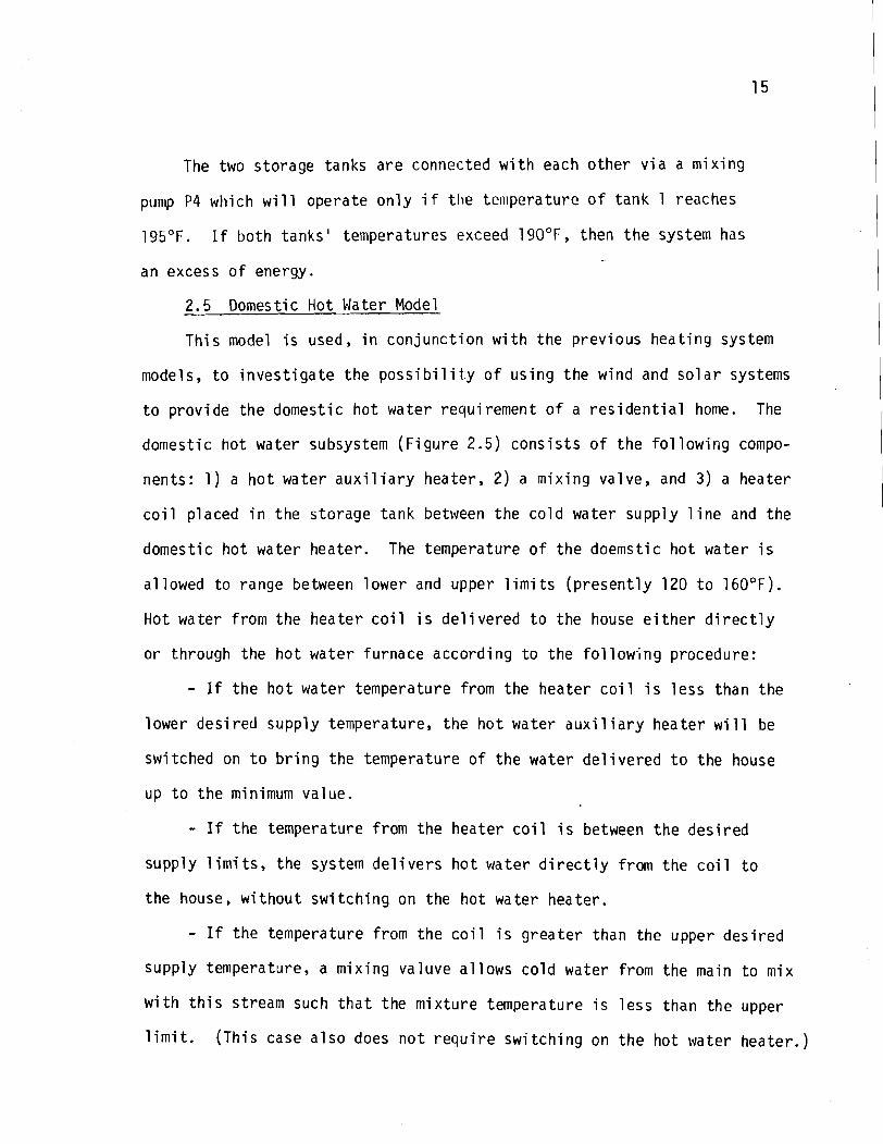
2.5 Domestic Hot Water Model

Th is model i s used, .in con junc t i on w i t h the prev ious heat ing system

models, t o i n v e s t i g a t e the p o s s i b i l i t y o f us ing the wind and s o l a r systems

t o prov ide the domestic ho t water requirement o f a r e s i d e n t i a l home. The

domestic ho t water subsystem (F igu re 2.5) cons i s t s o f t he fo l l ow ing compo-

nents: 1) a h o t water a u x i l i a r y heater, 2) a mix ing valve, and 3) a heater

c o i l placed i n the storage tank between the c o l d water supply l i n e and the

domestic ho t water heater. The temperature o f t he doemstic ho t water i s

al lowed t o range between lower and upper l i m i t s (p resen t l y 120 t o 160°F).

Hot water f rom the heater c o i l i s de l i ve red t o the house e i t h e r d i r e c t l y

o r through the h o t water furnace according t o the f o l l o w i n g procedure:

- I f the h o t water temperature from the heater c o i l i s l e s s than the

lower desi red supply temperature, the h o t water auxi 1 i a r y heater w i 11 be

switched on t o b r i n g the temperature of t he water d e l i v e r e d t o the house

up t o t h e minimum value.

- I f the temperature from the heater c o i l i s between t h e des i red

supply l i m i t s , the system d e l i v e r s h o t water d i r e c t l y from the c o i l t o

the house, w i thou t sw i t ch ing on the h o t water heater .

- I f the temperature from the c o i l i s g rea te r than the upper des i red

supply temperature, a mix ing valuve a l l ows co ld water from the main t o mix

w i t h t h i s stream such t h a t the m ix tu re temperature i s l ess than the upper

l i m i t . (This case a l s o does n o t r e q u i r e swi tch ing on the ho t water heater . )

C H A P T E R 3

SYSTEM COMPONENTS DESCRIPTION

The proposed wind and s o l a r heat ing system cons is t s o f t he f o l l o w i n g

bas ic components: 1 ) an e l e c t r i c a l wind generator, 2) a f l a t - p l a t e s o l a r

c o l l e c t o r , 3 ) a thermal energy storage tank, 4 ) a house, and 5) baseboard

heat exchangers. The o v e r a l l system performance i s a func t i on o f each

i n d i v i d u a l component. The f o l l o w i n g sect ions wi 11 i nc lude a d e s c r i p t i o n

of , and d e t a i l e d mathematical ana lys i s o f each o f the basic components

o f t h e var ious sytems.

3.1 The Windpower System

3.1.1 H i s t o r i c a l backqround

Energy from the wind i s n o t new t o the world. The Chinese and

t h e Japanese used w indmi l l s 4000 years ago. The Babylonians b u i l t a

w indmi l l system f o r t h e i r i r r i g a t i o n p ro jec ts . The f i r s t w indmi l l was

int roduced t o Western Europe i n the 12th century. (22) The e a r l y European

w indmi l l s were moved by s a i l s mounted on a h o r i z o n t a l ax is . The p rope l l e r -

type w indmi l l s t a r t e d a t the beginning of t h e 18th century. The new science

of aerodynamics and s t r u c t u r a l engineer ing con t r i bu ted t o t h e development

o f more powerful and e f f i c i e n t propel l e r - t y p e windmil 1 s. The advancement

o f w indmi l l s made poss ib le the conversion of windpower i n t o a more

v e r s a t i l e form - e l e c t r i c i t y . The f i r s t w ind -e lec t r i ca l generator was

b u i l t i n Denmark i n 1895 by Professor La Cour.

The l a r g e s t w i n d - e l e c t r i c a l generator b u i l t t o da te was the Smith-

Putnam machine s i t u a t e d i n Vermont (Uni ted Sta tes) . Th is 1250 kW machine

had a 175 f o o t diameter and was placed on a 110 f o o t tower. Thc machine

was designed t o feed a1 t e r n a t i n g cu r ren t power i n t o e x i s t i n g e l e c t r i c a l

networks. The present energy c r i s i s s t imu la ted more s tud ies t o develop

the technology o f wind energy conversion systems. For exarnple, a f e d e r a l

program (23) i s underway t o b u i l d a se r ies of l a r g e wind systems w i t h ra ted

capac i t i es rang ing from 100 kW t o several megawatts. Also, d e t a i l e d

s tud ies a re being performed t o determine the economical f eas i b i 1 i t y and

p u b l i c acceptance o f these systems. I n a d d i t i o n t o federal involvement

i n a n a l y t i c a l studies, a l a r g e 100 kW system was sponsored by ERDA and

b u i l t i n 1975 .at NASA-Lewis Research Center a t Plus Brook, Ohio. This

machine has a h o r i z o n t a l ax is , two bladed r o t o r (125 foo t diameter), and

mounted on a 100 foo t tower. (23) The wind machine i s used f o r generat ing

e l e c t r i c i t y and i t i s p resen t l y under t e s t . Experimental r e s u l t s w i l l be

used f o r f u t u r e designs o f l a r g e wind energy convers ion systems.

Another experimental windpower system i s under cons t ruc t i on a t t he

U n i v e r s i t y o f Massachusetts, a l s o sponsored by ERDA. Th is 25.0 kW wind

system has a th ree bladed r o t o r (32.5 f o o t diameter), h o r i z o n t a l ax is ,

and i s mounted on a 60 f o o t tower. Th is wind system i s used as p a r t o f an

experimental study on home heat ing us ing s o l a r and wind energy systems.

3.1.2 Windpower - basic fundamentals

Wind i s the mot ion o f a i r p a r t i c l e s caused by forces due t o , t he

Ear th 's ro ta t i on , buoyancy forces due t o g r a v i t y and s o l a r heat ing o f t h e

ground, and f r i c t i o n e x i s t i n g between a i r and the Ear th ' s surface. The

power i n the wind a t any moment i s the r e s u l t o f a mass o f a i r moving a t

a speed i n some p a r t i c u l a r d i r e c t i o n . Windpower can be computed using

Newton's Second Law and momentuln equat ions. Power i s equal t o energy

pe r t ime. The energy a v a i l a b l e i n t he wind i s t he k i n e t i c energy o f

t h e a i r p a r t i c l e s , and t o cap tu re t h i s energy, o r a f r a c t i o n o f i t , i t

i s necessary t o p lace i n t h e pa th a f t he wind a machine ( w i n d m i l l ) which

w i 11 r e t a r d t he wind and t r a n s f e r t i l e ava i l ab1 e power f rom t h e wind t o

t h e machine. Thus, t h e k i n e t i c energy i n t h e a i r i s t ransformed i n t o

mechanical o r e l e c t r i c a l power by wind genera to rs .

As w i l l be shown i n t he f o l l ow ing a n a l y s i s , t he amount o f power

which can be generated by a w i n d m i l l depends b a s i c a l l y on two f a c t o r s :

f i r s t , t h e wind speed, and second, t he area swept by t h e r o t o r .

The mass f l o w r a t e of a i r M pass ing through a r o t o r o f area A

(F igu re 3.1) i s

M = pAV (3.1)

where p = a i r d e n s i t y and V = a i r v e l o c i t y a t t he r o t o r . The k i n e t i c

energy a v a i l a b l e i n t he c o n t r o l s e c t i o n a t any i n s t a n t i s

The t h r u s t r e s u l t i n g a t t h e r o t o r due t o t he moving a i r stream i s

equal t o t h e r a t e o f change of t he momentum between s t a t e s 1 and 2.

where V 2 = downstream v e l o c i t y and V1 = upstream v e l o c i t y . The power

exchange by t he r o t o r i s equal t o t he r a t e of change i n k i n e t i c energy:

FIGURE 3.1 - Windmill Rotor and Velocities.

Also, power i s equal t o the t h r u s t exerted by t h e w indmi l l t imes the

mean f l o w through the r o t o r . Thus

Equations 3.4 and 3.5 a re obv ious ly equal so t h a t -

f rom which

1 V = $V2 + V1)

Equation 3.6 could be w r i t t e n as fo l l ows

v l - v = v - v 2 (3.7)

which means t h a t r e t a r d a t i o n o f the v e l o c i t y upstream i s equal t o

r e t a r d a t i o n downstream.

S u b s t i t u t i n g f o r V i n Equation 3.4 and us ing non-dimensional

2 v e l o c i t i e s , by l e t t i n g B = g, we g e t 1

1 3 2 P = pAV1(l + B)(1 - B (3.5)

The maximum power f o r a g iven wind speed, V1, i s obtained by d i f f e r e n -

aP t i a t i n g Equation 3.8 w i t h respect t o 6 and s e t t i n g = 0. This y i e l d s

Therefore, the power P i s maximum when the downstream v e l o c i t y V 2 i s one

t h i r d the upstream v e l o c i t y V1. Thus, the maximum power which can be

ex t rac ted from the wind i s

The maximum t h e o r e t i c a l power as a percent of the t o t a l a v a i l a b l e

power i s c a l l e d " the maximum power c o e f f i c i e n t "

- '"ax - 16 - 59.3% C ~ - ~ - - - 2 7 (3.10)

which means t h a t an i dea l windmi 11 can e x t r a c t 59.3 percent o f the

power i n the wind. Cp i s a f u n c t i o n o f the design o f the r o t o r .

3.1.3 Power losses

A p rope l l e r - t ype w indmi l l e x t r a c t s l e s s power than the maximum

due t o t h e f a c t t h a t t he re i s a component o f a i r f l o w along the r a d i u s

adjacent t o t h e blade paths which r e s u l t s i n an exchange o f a i r f l o w

around the blade t i p s w i t h a consequent t i p loss. The theory i n the

previous sec t i on d i d n o t account f o r the aerodynamics losses ( t i p l oss )

due t o t h e shape and s t r u c t u r e o f t he w indmi l l , t h e mechanical f r i c t i o n

losses i n the gear ing and the bearings, and generator losses.

The aerodynamic e f f i c i e n c y , qa, of the w indmi l l depends on the

shape o f t he blade and the d i r e c t i o n o f wind r e l a t i v e t o the blade.

Suppose t h a t a blade element i s placed so t h a t i t w i l l make an angle

(a + 9 ) w i t h the d i r e c t i o n o f the wind (F igure 3.2). The wind v e l o c i t y

approaching the element V w i l l c rea te forces t h a t w i l l cause t h e b lade

t o r o t a t e w i t h a tangen t ia l v e l o c i t y v perpendicular t o V . V R i s the wind

r e l a t i v e v e l o c i t y and makes an angle a w i t h the blade element surface.

Fb i s the f o r c e a c t i n g on the sur face o f t h e blade and has two components --

a l i f t f o r c e Lf perpendicular t o t h e r e l a t i v e v e l o c i t y and a drag f o r c e Df

p a r a l l e l t o the same v e l o c i t y . Also, Fb could be s p l i t i n t o two d i f f e r e n t

components, a t h r u s t T i n the d i r e c t i o n o f the wind v e l o c i t y V and a

d r i v i n g force TD i n t h e d i r e c t i o n of motion o f the blade. The r e l a t i o n s

between T, TD, Lf and Df are g iven i n the fo l l ow ing equations.

FIGURE 3 . 2 - Wind V e l o c i t i e s and Forces a t a Blade Element.

if k i s the r a t i o f, then f

where v i s the tangen t ia l v e l o c i t y . The d e f i n i t i o n o f aerodynamic

e f f i c i ency na o f t he w indmi l l machine i s the r a t i o o f t he use fu l power

TD.v t o the power a r r i v i n g a t the machine TsV v TD*v 1 - kv

- - - - - (3.16)

where i s c a l l e d the t i p speed r a t i o . The power output o f the w indmi l l v machine i s o f f s e t by TJ,, (mechanical e f f i c i ency ) due t o mechanical losses,

such as, bear ing f r i c t i o n , brush f r i c t i o n , and wind f r i c t i o n -- u s u a l l y

c a l l e d windage. Also, t he generator e l e c t r i c a l losses, hys teres is , eddy

cur rents , and res is tance heat ing losses reduce the power output by 11 9

( t h e generator e f f i c i e n c y ) . nq i s the r a t i o of the e l e c t r i c a l power - ou tpu t t o the mechanical power i npu t . (24)

The t o t a l e f f i c i e n c y of t he w indmi l l machine i s g iven by

n = n a - ng ' nm (3.17)

Using Equation 3.9, t he useful power output o f t he machine i s g iven by

3 Pu = 0.296npAV1 (3.18)

Th is imp l ies t h a t t he useful power output o f a wind generator i s a

D2 f u n c t i o n o f t he wind v e l o c i t y and the generator blade diameter (A = T ~ ) .

WIND S P E E D , M P H

! FIGURE 3.3 - The Wind Generator Performance Curves.

Therefore, f o r a g i ven wind data, t h i s a n a l y t i c a l model c a l c u l a t e s t h e

use fu l power o u t p u t o f t h e genera to r as a f u n c t i o n o f b lade d iameter

and wind v e l o c i t y .

The n e t power o u t p u t of t h r e e b laded machines f o r t h i s system a r e

presented i n F i g u r e 3.3, as a f u n c t i o n o f t h e wind speed and b lade d iameter .

These gene ra l i zed performance curves a r e based on t h r e e a n a l y t i c a l programs

developed a t t he U n i v e r s i t y of Massachusetts. The a n a l y t i c a l programs

i n c l u d e wind genera to r and b lade element ( s t r i p ) t h e o r y and a r e based

on s tandard w i n d genera to r and aerodynamics p r a c t i c e . (25926) A comparison

between t he t h e o r e t i c a l , based on Equat ion 3.18, and a n a l y t i c a l power ou tpu t

o f t h e w i n d genera to r i s shown i n F i g u r e 3.4. The t h e o r e t i c a l r e s u l t s a re

based on t h e f o l l o w i n g assumptions: o v e r a l l e f f i c i e n c y q = 1; d e n s i t y

3 o f a i r a t 70°F p = .0735 Lbc! / f t and a b lade d iameter D = 32.5 f e e t .

Wind speed i s a f u n c t i o n o f he igh t . Therefore, when c a l c u l a t i n g

windpower o u t p u t (and a l s o o u t s i d e convec t i ve hea t t r a n s f e r c o e f f i c i e n t s ) ,

wind speed f rom a v a i l a b l e data i s c o r r e c t e d f o r t h e cor respond ing h e i g h t

by usi.ng Hel lman's r e l a t i o n : (26

V s = vl0[0.2337 + 0.656 l0gl0(Y + 4 .75) ] (3.19)

where :

V10 = wind speed a t 10 meters above ground

VS = w ind speed a t S f e e t above ground

Y = S f e e t expressed i n meters

3.2 The F l a t - P l a t e C o l l e c t o r Subsystem

3.2.1 S o l a r r a d i a t i o n - i n p u t

Energy e m i t t e d from t h e sun i s i n t h e f o rm o f e lec t romagnet i c r a d i a t i o n .

WIND SPEED, m p h

FIGLIRE 3.4 - Coniparison of t h e A n a l y t i c a l and T h e o r e t i c a l Curves o f t h e Wind Genera to r (D = 32.5 ft. ).

Outs ide the atmosphere t h e spec t ra l i n t e n s i t y o f t he s o l a r r a d i a t i o n

i s centered near t h e v i s i b l e p o r t i o n o f the e lec t romagnet ic spectrum

and ranges from 0.3 t o 3 microns. The shape o f the s o l a r spectrum

corresponds t o the emiss ion spectrum o f a b lack body, i n d i c a t i n g t h a t

t h e sun can be approximated by a b lack body r a d i a t o r . Also, some o f t h e

s o l a r r a d i a t i o n i s sca t te red and absorbed by t h e d r y a i r molecules, t h e

d u s t p a r t i c l e s present i n t h e a i r , water vapor p a r t i c l e s , and t h i n

c loud l a y e r s . Furthermore, t h e exac t amount o f d i r e c t s o l a r r a d i a t i o n

( a t a s i t e ) depends on t h e a1 t i t u d e and t h e sun 's z e n i t h ang le a t t h e

speci f i ed 1 oca t i on.

So la r data u s u a l l y c o n s i s t s of hou r l y measurements o f i n s o l a t i o n

on a surface a t a c e r t a i n l o c a t i o n . For example, t h e i n i t i a l da ta used

i n t h i s model were the t o t a l s o l a r i n s o l a t i o n on a t i l t e d sur face ' (60

degrees from' t h e h o r i z o n t a l ) measured a t t he MIT So la r House I V a t B lue

H i l l s , Massachusetts. (27 )

3.2.2 The F l a t - P l a t e C o l l e c t o r

A convent iona l f l a t - p l a t e s o l a r c o l l e c t o r i s used i n t h i s model.

The c o l l e c t o r faces the equator , and i t inc ludes a f l a t b lack m e t a l l i c

p l a t e and i s i n s u l a t e d on the back s i d e t o reduce, heat losses. A number

of a i r spaced g laz ings ( two i n t h i s model) a r e used as a cover (F igu re 3.5).

The cover p l a t e s a l l o w s h o r t wave s o l a r r a d i a t i o n t o come through and a re

designed t o be opaque t o l ong wave hea t r e - r a d i a t i o n from t h e c o l l e c t o r

p l a t e . The s o l a r energy absorbed ( i n a form o f heat) by t h e blackened

p l a t e i s removed by a work ing f l u i d (water) c i r c u l a t e d through tubes

soldered t o t h e c o l l e c t o r p l a t e .

ADSORBER TWO GLAZINGS

F R A M E TlJ BE S

FIGURE 3.5 - Flat Plate col lector Design.

The useful energy collected i s the dif ference between the

r a t e a t which so l a r energy i s absorbed by the blackened p la te and the

r a t e a t which heat i s l o s t from the co l lec tor due t o convection and re-

radia t ion losses from the col lector t o the surrounding a i r . In the

following sect ions the various sectors of the co l l ec tor model ( inso la t ion ,

heat losses , radia t ion losses , e t c . ) will be discussed.

The Collector Model

The to ta l s o l a r insolat ion I on a surface i s the sum of the d i r ec t

component Id and the diffused (sky) corr~ponent Is of the s o l a r radiation

1 = 1 + I d s (3.20)

The intensi ty of the so l a r insolat ion ona surface var ies with the

location and or ientat ion of the surface, time of the day, and the cloud

cover. To use the avai lable so l a r data f o r insolat ion on a t i l t e d

surface, the following r e l a t i ons f o r a ver t i ca l surface must be used.

The d i r ec t insolation on a t i 1 ted surface i s given by

and the d i r e c t so l a r insolat ion on a ver t ical surface Id equals

- cos i Id - Idt cos i l

i and i l a r e the incidence angles on ver t ica l and' t i l t e d surfaces

respectively. The sky so l a r radia t ion, I s , i s based on a multiple

regression analysis of data taken over several thousand hours. (12)

I, = 0.78 + 61.3e + 6.17CC (3.23)

CC = cloud cover ( sca le : 0 t o 10; where 0 i s c l ea r and 10 i s cloudy),

e = s o l a r elevation above the horizon in radians.

The angle o f inc idence o f s o l a r r a d i a t i o n on any sur face i s obta ined (28)

by means o f t he f o l l o w i n g :

cos i = ( s i n L cos B - cos L s i n B cos PS) s i n d +

(cos L cos B + s i n L s i n B cos PS)cos d cos H + s i n B

s i n P, cos d s i n H (3.24)

o r from:

cos i = s i n Aacos B + s i n Aasin B cos(Z - Ps)

(3.25)

L = La t i t ude , B = T i l t angle f rom t h e sur face t o t h e h o r i z o n t a l , Ps =

Surface azimuth, Z = So la r azimuth, d = Dec l ina t ion , H = Hour angle,

A, = s o l a r a l t i t u d e .

TI For t h e spec ia l case o f a v e r t i c a l c o l l e c t o r B = 7 and Equations

3.24 and 3.25 reduce t o

cos i = s i n L cos Ps cos d cos H + s i n Ps cos d s i n H

- cos L cos P, s i n d (3.26)

cos i = cos Aacos (Z - Ps) (3.27)

3.2.4 R e f l e c t i o n Losses

A1 1 t h e i n c i d e n t s o l a r r a d i a t i o n i s n o t t ransmi t ted t o the absorber

p l a t e ; p a r t of t he r a d i a t i o n i s r e f l e c t e d back t o t h e sky. These r e f l e c t i o n

losses a r e discussed i n t h e fo l l ow ing .

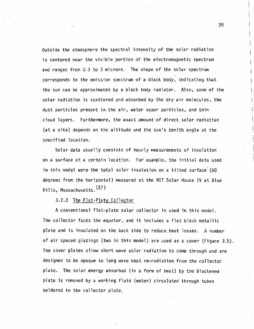
A. R e f l e c t i o n o f d i r e c t r a d i a t i o n from a s i n g l e sur face o f g lass

i s g i ven by Fresnel ' s equat ion (12)

1 s i n 2 ( i - r ) + t a n 2 ( i - r ) ] R l = 9 2 2 (3.28) s i n ( i + r ) t an ( i + r )

where R1 = f r a c t i o n re f l ec ted , r = r e f r a c t i o n angle, i = inc idence

angle. The r e l a t i o n between the r e f r a c t i o n angle and the angle o f

inc idence i s g iven by S n e l l ' s law (F igure 3.6)

"2 - s i n i - - - nl s i n r

"1 ' n2 a r e the r e f r a c t i o n ind ices f o r the two media. The t o t a l f r a c t i o n

o f the s o l a r r a d i a t i o n r e f l e c t e d due t o N number o f glass covers i s

RN i s ca lcu la ted based on the assumption t h a t no r a d i a t i o n i s absorbed

by the cover p la tes .

0 . Ref lected sky r a d i a t i o n : In a d d i t i o n t o the r e f l e c t i o n losses

o f the d i r e c t r a d i a t i o n some of the sky r a d i a t i o n i s r e f l e c t e d due t o the

f a c t t h a t sky r a d i a t i o n cons is ts i n p a r t o f d i r e c t r a d i a t i o n coming from

a l l pa r t s of the hemisphere. This r e f l e c t i o n loss Rr was ca lcu la ted as

a func t ion o f the number o f cover p la tes by means o f g raph ica l i n t e g r a t i o n

over a uniform hemispheric sky, g iven i n Table 3 .l. (12) Therefore, the

t o t a l energy t ransmi t ted through the g lazings per u n i t area qt, i s equal

t o t h e t o t a l r a d i a t i o n on the c o l l e c t o r minus the r e f l e c t i o n losses and

i t i s g iven by the f o l l o w i n g equation:

3.2.5 Absorpt ion Losses

Par t o f the t ransmi t ted s o l a r r a d i a t i o n s reaching the absorber p l a t e

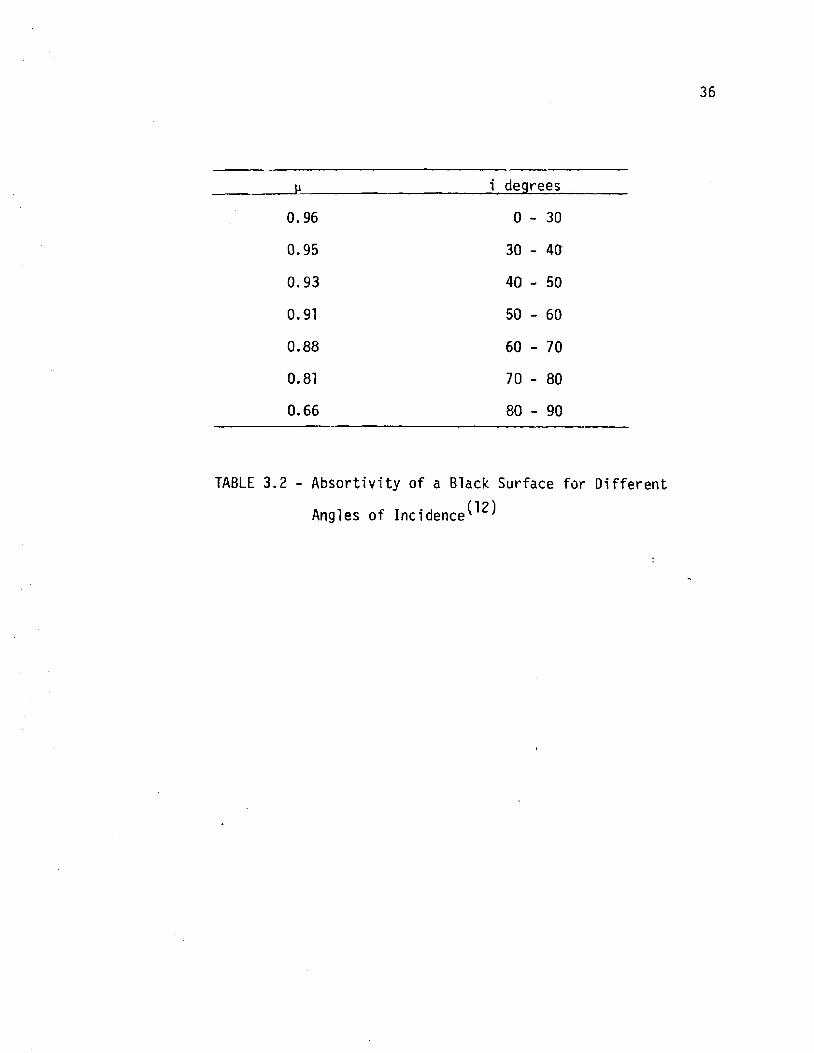
i s n o t absorbed. The amount absorbed i s a funct ion of the a b s o r t i v i t y o f

the p l a t e surface which i s discussed i n the fo l lowing.

FIGURE 3.6 - Illustration of Snell's Law.

TABLE 3.1 - R e f l e c t i o n C o e f f i c i e n t o f D i f f u s e d

R a d i a t i o n f o r Var ious Numbers o f

Gl az ings (12)

For d i r e c t s o l a r r a d i a t i o n a non-se lec t ive b lack sur face has an

absorp t ion c o e f f i c i e n t p . Th i s v a r i a b l e i s a func t i on o f t he inc idence

angle and g iven i n Table 3.2. The absorp t ion c o e f f i c i e n t f o r the d i f f u s e d

r a d i a t i o n can be found by i n t e g r a t i n g absorp t ion as a f unc t i on of

inc idence angle over hemispher ica l .sky f o r an average value. This

average value i s 80 percent o f the d i f f used component o f the t ransmi t ted

s o l a r r a d i a t i o n . Therefore, t h e t o t a l useful r a d i a t i o n absorbed by the

b lack p l a t e per u n i t area qa i s equal t o t he t ransmi t ted r a d i a t i o n minus

the absorp t ion losses :

qa = I d ( l - RN)p + I S ( l - Rr)(0.90) (3.32)

t he f o l l o w i n g assun~ptions were made by ob ta in ing qa: (") 1 ) no d i r t

on t h e g laz ings; 2) no shading e f f e c t f rom the s ides o f t h e c o l l e c t o r on

the absorber p la te ; 3) t h e energy r e f l e c t e d f rom the absorber p l a t e i s

complete ly t ransmi t ted by t h e g laz ings ; 4) no mois ture on the g laz ings .

3.2.6 Heat Losses from the Absorber P l a t e

The convect ive heat losses per u n i t area qc from the absorber p l a t e

sur face t o the f i r s t g lass cover a r e g iven by (29)

qc = hcl (Tp - Tgl (3.33)

where T + T a r e the temperatures of the c o l l e c t o r and the f i r s t g lass P g l

p la te , respec t i ve l y . hcl i s t h e convect ive heat t r a n s f e r c o e f f i c i e n t

between two p a r a l l e l t i l t e d p l a t e s g iven by

= C U P - Tgl) 1 /4 hc l (3.34)

where C i s dependent on the t i lt angle and i t i s found from (11)

C = 0.19 - 7.78 x I O - ~ B (3.35)

B i s t he t i lt angle i n degrees.

P i degrees

0.96 0 - 30

0.95 30 - 40

0.93 40 - 50

0.91 50 - 60

0.88 60 - 70

0.81 70 - 80

0.66 80 - 90

TABLE 3.2 - Abso r t i v i t y o f a Black Surface for D i f f e ren t

Angles o f Incidence (12)

The r a d i a t i v e heat losses between two l a r g e p a r a l l e l p l a t e s a re

a f u n c t i o n of t he e m i s s i v i t y , ec of the c o l l e c t o r sur face and e o f t he 9

g lass p l a t e , and the temperatures o f t h e p l a t e s are g iven by:

where Ecg = ( 1 + - and u = Stefan-Boltzmann constant . The

9 t o t a l r a t e o f heat l o s s qL from the c o l l e c t o r p l a t e t o the f i r s t g lass p l a t e

i s the sum o f the r a d i a t i v e and t h e convect ive losses

S i m i l a r l y t h e same heat l o s s qL occurs between t h e f i r s t and second

p la tes .

which i s equal t o t he heat l o s s between the second p l a t e and the

surrounding a i r

where hc i s t he o u t s i d e convect ive c o e f f i c i e n t .

Given the c o l l e c t o r temperature and t h e ou ts ide a i r temperature, t he

c o l l e c t o r heat losses qL cou ld be found by s o l v i n g the equat ions f o r qL

s imul taneously. This s o l u t i o n , however, i s ve ry complicated and requ i res

cons iderab le computat ional e f f o r t . An approximate s o l u t i o n f o r qL was

found by H o t t e l and Woertz (29) which was mod i f i ed l a t e r by ~ l e i n ' ~ ~ ) and

i s expressed by:

2 With qL in un i t s of watts/m2 f = (1 - 0.04hc + 0.0005hc)(l + 0.091N);

hc = 5.7 + 3.8Vm, ( h c = w / ~ ' K and V, = rn/sec); C = 365.9(1 - 0.008838 +

0 .0001298~~) ;0 5 B 5 90° ( t i l t ) . In t h i s model i t i s assumed tha t there

a r e no edge and rear losses , and tha t the absorbed so l a r energy r a t e

per uni t area is constant over each hour.

3.2.7 Overall Col 1 ec tor Enerqy Balance

Using a control volume (C.V. 1 ) around the absorber pla te bs shown

i n Figure 3.7) one can write the following energy balance equati0.n:

Net r a t e of energy in = Rate of energy stored

which yields to the following:

qa - qL = Elc C 1 5 d t

where M, i s the mass per un i t area of the absorber and re ta ining plate

system, C1 i s the spec i f ic heat of the co l lec tor system and t i s time.

Assuming the col lector t o be operating in steady s ta te , the rate of net

so l a r energy transferred t o the ci rculat ing water through col l ec tor ,

Us , i s obtained from the control volume (C.V.2) around the absorber

pla te (Figure 3 .7) .

where Ac i s the col lector area, Mw the mass f l o w r a t e of water through

the co l lec tor , C i s the specif ic heat of water, Tout and T i n a r e the P

ou t l e t and i n l e t temperature of the water respectively, E the r a t e of

useful energy per u n i t area of the col lector .

In case the control volume will have unsteady conditions, such as

a varying i n l e t temperature of the water, Equation 3.42 should contain a

term tha t accounts for the change in the col lector temperature which

S O L A R ENERGY R E F L E C T E D SOLAR R A D I A T I AT ION

r 1

GLAZING @

H E A T LOSS

L

- -

- I

m,7 - - - - - - - - - - - - - - - - - - T~~ ABSORBER PLATE

FIGURE 3.7 - F l a t P l a t e So la r Co l l ec to r .

r e s u l t s i n :

(qa - qL )d t - Edt = McCldtp

I n t e g r a t i n g the l a s t equat ion w i t h the assumption t h a t t he c o l l e c t o r

operates a t a steady s t a t e d u r i n g one hour i n t e r v a l s we o b t a i n the

fo l l ow ing :

which completes the bas ic a n a l y t i c a l model Tor the s o l a r c o l l e c t o r .

3.3 Energy Storage

3.3.1 Background

Since n e i t h e r wind nor s o l a r r a d i a t i o n i s a v a i l a b l e a l l t he time,

energy storage i s a c r u c i a l f a c t o r i n opera t ing a s o l a r heat ing o r coo l i ng

system. Storage o f windpower and s o l a r energy cou ld be achieved through

d i f f e r e n t methods such as, e l e c t r o l y s i s o f water which s to res energy

i n the form o f hydrogen, DC b a t t e r i e s , f lywheel storage, pumped water

storage, compressed a i r storage, o r thermal energy storage. I n the

present system, thermal energy was chosen as the most appropr ia te .

Thermal energy i s accumulated as s p e c i f i c heat (sens ib le heat) o r as

heat of fusion ( l a t e n t heat) . I n many cases the use o f water proves t o be

the most favo ra t l emate r ia l t o work w i t h f o r economical and a v a i l a b i l i t y

purposes. The thermal energy storage f o r the present system

i s based on the use o f a w e l l i nsu la ted concrete water tank w i t h e l e c t r i c

heaters o r heat exchangers submerged i n s i d e the tanks. This system i s

located i n t h e basement of the house and supp l ies heated water t o the

house heat ing u n i t s (baseboard heaters) .

3.3.2 Storage A n a l y t i c a l Model

The energy balance equa t i on f o r t h e c o n t r o l volume a r - , ' t h e

s torage tank (F igu re 3.8) takes i n t o account t h e r a t e o f c- .jy l o s t

f rom the tank t o t h e surrounding Qtl, t h e r a t e o f s o l a r energy c o l l e c t e d . Q,, t h e r a t e o f use fu l windpower Q,, t h e r a t e o f energy supp l i ed t o t h e

house by t he baseboard heaters Qb, and t h e r a t e o f energy change i n t h e

s to rage tank i t s e l f , Qst:

where

dTs Q s t = MsCp z-

M,, Cp, T, a r e t h e mass, s p e c i f i c heat, and t h e temperature o f t h e

s to rage water r e s p e c t i v e l y . The thermal l o s s th rough t h e t ank w a l l s

Qtl i s g i ven by:

AS = t ank sur face area, Tr = room temperature, Us i s t h e o v e r a l l heat

t r a n s f e r c o e f f i c i e n t o f t h e tank g i ven by

hi a r e t h e o u t s i d e and i n s i d e convec t i ve heat. t r a n s f e r c o e f f i c i e n t s .

Th and \ a r e t h e t h i ckness and thermal c o n d u c t i v i t y o f t h e tank w a l l s

r e s p e c t i v e l y . The r a t e a t which energy i s supp l i ed t o t h e house by t h e

baseboard heaters Qb i s :

where Mb, Tb a r e t h e f l o w r a t e and temperature o f t h e baseboard heaters

r e s p e c t i v e l y .

The r a t e o f use fu l s o l a r energy c o l l e c t e d Q, i s g i ven by:

I n t e g r a t i n g Qs, Qb and Qst w i t h t h e assu l i~p t ion t h a t temperatures a r e

cons tan t o v e r a p e r i o d o f one hour we g e t :

and

Subsc r i p t s ( 1 ) and ( 2 ) r ep resen t t he i n i t i a l and f i n a l temperatures

r e s p e c t i v e l y .

I f t h e s to rage tank were used as a p re -heat f o r domest ic h o t water

demand Equat ion 3.46 w i l l have an a d d i t i o n a l te rm Qhw.

where

Qhw = MhwCp(Ts -

Qhw = the r a t e o f energy t h a t t h e system c o u l d supp ly f o r domest ic h o t

water use. Mhw = t he mass f l o w r a t e o f domestic h o t water f rom t h e s to rage

tank. Tcw = c o l d water temperature.

The domestic h o t water requi rements f o r a f a m i l y o f f o u r i s g i ven

i n Table 3,3.

3.4 The House

3.4.1 Res iden t i a l Homes

Two d i f f e r e n t houses a r e s in iu la ted i n t h e computer program -- a "r40delfl

house and an "Average" one. The "Model" house i s based on Pro fessor C u r t i s

1 TOTAL 50.00

- Hot Water

Gal l ons

TABLE 3.3 - D a i l y Domestic Hot Water Demand (5 )

Time Hot Water Gal 1 ons

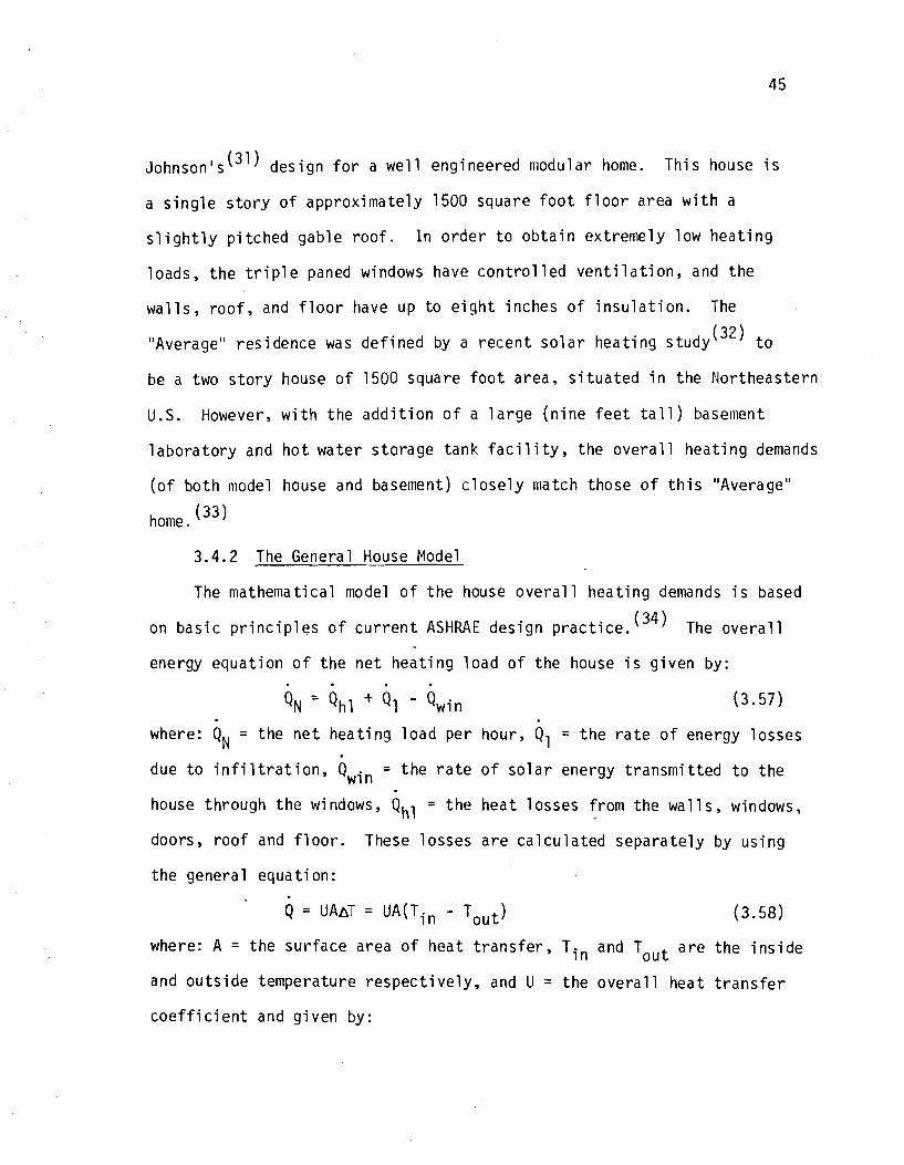
~ o h n s o n ' s ( ~ ~ ) des ign f o r a w e l l engineered nlodular home. Th i s house i s

a s i n g l e s t o r y o f approx imate ly 1500 square f o o t f l o o r area w i t h a

s l i g h t l y p i t c h e d gab le r o o f . I n o r d e r t o o b t a i n ex t reme ly low h e a t i n g

loads, t h e t r i p l e paned windows have c o n t r o l l e d v e n t i l a t i o n , and t h e

w a l l s , roo f , and f l o o r have up t o e i g h t inches o f i n s u l a t i o n . The

"Average" res idence was d e f i n e d by a r e c e n t s o l a r hea t i ng s tudy (32) to

be a two s t o r y house o f 1500 square f o o t area, s i t u a t e d i n t he Nor theas te rn

U.S. However, w i t h t h e a d d i t i o n o f a l a r g e ( n i n e f e e t t a l l ) basement

l a b o r a t o r y and h o t wa te r s to rage tank f a c i l i t y , t h e o v e r a l l h e a t i n g demands

( o f b o t h model house and basement) c l o s e l y match those o f t h i s "Average"

home. (33)

3.4.2 The General House Model

The mathematical model o f t h e house o v e r a l l h e a t i n g demands i s based

on b a s i c p r i n c i p l e s o f c u r r e n t ASHRAE des ign p r a c t i c e . ( 3 4 ) The o v e r a l l

energy equa t i on o f t h e n e t h e a t i n g l o a d of t he house i s g i ven by:

- QN - Q ~ I + QI - Qwin

where: QN = t h e n e t h e a t i n g l o a d p e r hour, Q1 = t h e r a t e o f energy losses

due t o i n f i l t r a t i o n , Qwin = t h e r a t e o f s o l a r energy t r a n s m i t t e d t o t h e

house th rough t h e windows, Qhl = t h e hea t l osses f rom t h e w a l l s , windows,

doors, r o o f and f l o o r . These losses a r e c a l c u l a t e d s e p a r a t e l y by us ing

t h e genera l e q u a t i on:

where: A = t h e su r f ace area of hea t t r ans fe r , Tin and Tout a r e t h e i n s i d e

and o u t s i d e temperature r e s p e c t i v e l y , and U = t h e o v e r a l l hea t t r a n s f e r

c o e f f i c i e n t and g i ven by:

where: ho, hi a r e the outs ide and i n s i d e convect ive heat t r a n s f e r

c o e f f i c i e n t s respec t i ve l y , Th and K a re the th ickness and thermal

c o n d u c t i v i t y o f the surface. hi and K a re assumed t o be a f u n c t i o n o f

the house design and constant i n t ime. However, t h e outs ide convect ion

c o e f f i c i e n t , ho, i s a func t ion of wind v e l o c i t y and d i r e c t i o n . For

wind blowing p a r a l l e l t o the w a l l , assuming a constant Prandt l number

5 t h e average convect ion c o e f f i c i e n t KO i s found from the f o l l o w i n g

equat ion : (35,361 - K a i r 0.5

Laminar Region: ho = 0.664 *ex Prai 33 For ~ e ~ 1 5 0 0 , 0 0 0

o r (3.60) - K a i r 0.33

Turbulent : ho = 0.036 -----Prair ( ~ e ~ ' ~ - 2 3 2 0 0 ) For Rex>500 ,000 X

(3.61 )

where x = t h e l e n g t h o f the w a l l ; Rex = Reynolds number as f u n c t i o n o f

v X x, and def ined by Rex = y- where V i s the wind v e l o c i t y and v t he k inemat ic

v i s c o s i t y ; Kair = Thermal c o n d u c t i v i t y of a i r . For wind b lowing i n t o

t h e w a l l , assuming a constant Pr and t h a t the f l o w i s always i n t h e

laminar region, KO i s g iven by:

when the wind d i r e c t i o n i s perpendicular t o one w a l l i t i s assumed t o

be p a r a l l e l t o the o the r w a l l s . The basement heat losses a re assumed

t o be independent o f t h e wind v e l o c i t y and d i r e c t i o n except f o r t he pa r t s

t h a t a r e exposed t o the wind. The ground temperature i s considered t o vary

l i n e a r l y from 50°F a t the basement f l o o r l e v e l t o the ou ts ide a i r

temperature a t ground l e v e l ,

The heat losses due t o a i r i n f i l t r a t i o n account f o r a s i g n i f i c a n t

p o r t i o n o f the t o t a l heat losses of the house. A i r i n f i l t r a t i o n i s due

t o d i f f e rences i n pressure and dens i t y between the i n s i d e and ou ts ide

o f t he house. Wind b lowing aga ins t t he house causes'an increase i n t h e

ou ts ide pressure and a p a r t i a l vacuum on the leeward s ide o f t h e house.

Thus, t o reduce the pressure d i f fe rence co ld a i r f lows i n and warm a i r

f lows out . A i r dens i t y d i f ferences a re i n s i g n i f i c a n t f o r s h o r t b u i l d i n g s

and a re n o t considered i n t h i s model. I n general t he re a re two methods

t o est imate a i r i n f i l t r a t i o n i n a house: 1 ) t h e d e t a i l e d crack method ( 34 )

which i s based on measuring the leakage c h a r a c t e r i s t i c s o f the house components

and selected pressure d i f fe rences; o r 2 ) t h e a i r changes method which assumes

a number o f a i r changes per hour f o r each room. The number o f changes i s

dependent on the type, use and l o c a t i o n o f the room. (34)

Since the model house was designed f o r c o n t r o l l e d a i r v e n t i l a t i o n ,

the second method i s used i n t h i s model. Thus, t h e i n f i l t r a t i o n heat losses

Qi i s g iven by the f o l l o w i n g equation:

- Qi - pCairVi (Tr - Ta) (3.63)

where Qi = i n f i l t r a t i o n heat losses per hour; P and Cair a re the dens i t y

and s p e c i f i c heat of a i r respec t i ve l y ; Vi i s the vo lumet r ic f l o w r a t e

per hour. As recormiended by ASHRAE, (34) t o keep l i v i n g cond i t i ons i n the

house comfortable, the volumetr ic f low r a t e of a i r i s considered t o be

one volume'change per hour.

The so la r energy coming i n t o the house through the windows, Qwin. warms

the a i r i n s i d e the house and c o n t r i b u t e s t o the reduc t ion o f t h e house

t o t a l heat ing load. Most types of a r c h i t e c t u r a l g lass a r e completely

opaque t o longwave r a d i a t i o n s em i t t ed by sur faces a t temperatures l e s s

than 250°F. Thi s c h a r a c t e r i s t i c produces t h e greenhouse e f f e c t ( s o l a r

r a d i a t i o n which en te rs th rough t h e windows i s t rapped i n s i d e t h e house).

S o l a r r a d i a t i o n s absorbed by surfaces i n s i d e t h e house a r e emi t ted as

heat ( longwave r a d i a t i o n s ) which cannot escape outward s ince windows

a r e opaque t o a l l r a d i a t i o n s w i t h wave l e n g t h beyond 3.0u. Qwin i s

c a l c u l a t e d by us ing an approach s i m i l a r t o t h a t o f t he s o l a r c o l l e c t o r

and i t i s g iven by:

- Qwin - qaAwin( '

where: qa = absorbed s o l a r energy per u n i t area; AWin = area o f t h e

windows f a c i n g the sun; SHADE - shade fac to r . S o l a r energy through

the windows i s c a l c u l a t e d f o r windows t h a t t he sun shines through on ly .

The n e t hea t i ng l oad the re fo re i s t h e t o t a l hea t i ng requirements o f

t h e house minus the s o l a r energy transmi t t e d t o t h e house th rough t h e

windows . 3.5 The Heat D e l i v e r y Model

The r a t e a t which energy i s t r ans fe r red t o t h e house i s dependent

on t h e s i z e and c h a r a c t e r i s t i c s o f t h e heat exchanger used. I n t he

corr~puter model, t h e hea t i ng system i s t e s t e d f o r t he f o l l o w i n g two cases:

1 ) a counter f l o w heat exchanger o f a f i n i t e s i z e (F igu re 3.9) which

d e l i v e r s energy t o t h e system as a f u n c t i o n o f i t s e f f ec t i veness . The

exchanger heat t r ans fe r e f fec t i veness E , i s def ined by t h e f o l l o w i n g

equat ion:

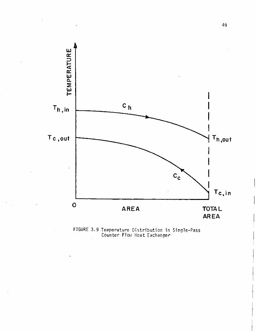
A R E A

F I G l l R E 3 . 9 Temperature Distribution i n Single-Pass Counter Flow tleat Exchanger'

TOTA L AR €A

FIGURE 3.10 - Counter-Flow Heat Exchanger.

where Qb = t h e ac tua l heat t rans fe r r a t e ; Qmax = maximum poss ib le heat

t r a n s f e r r a t e . Th and Tc a r e the h o t and c o l d f l u i d te rmina l temperatures

r e s p e c t i v e l y . Ch = (mC ) t he h o t f l u i d capac i t y ra te . For our case P h

'mi n = Ch f o r a coun te r f l ow exchanger, F igu re 3.10, Since the c o l d f l u i d

i s a i r i n s i d e the house (Cc i s g r e a t e r than C h ) 2 ) an i n f i n i t e heat

exchanger w i t h E = 1.

The e f f e c t i v e n e s s cou ld a l s o be w r i t t e n as a func t ion o f t he number

o f heat t r a n s f e r u n i t s (NTU) and the f l u i d capac i t y r a t e s (37) and i t i s

g iven by:

- where Cmin - - 'max - Cc, t h e c o l d f l u i d capac i t y r a t e and NTU =

, where A = area o f heat exchanger and U = i t s o v e r a l l heat t r a n s f e r 'mi n c o e f f i c i e n t .

Since heat i s t r a n s f e r r e d t o the a i r i n t he house, t h e a i r capac i t y

r a t e i s much l a r g e r than the h o t f l u i d capac i t y r a t e , >> and

/ C = 0, there fore the e f f e c t i v e n e s s equat ion y i e l d s : 'min max

€ = + I - e - NTU

From t h i s equat ion one can show t h a t t he e f fec t i veness o f an i n f i n i t e

area heat exchanger i s equal t o one. One cou ld c a l c u l a t e the ac tua l

heat d e l i v e r e d t o the house Qb, by s p e c i f y i n g the f low r a t e of t he h o t

f l u i d , t h e heat exchange area, A, and the o v e r a l l heat t r a n s f e r c o e f f i c i e n t

o f t he exchanger, U. If t h e heat exchanger f a i l s t o supply a l l the heat ing

load, an a u x i l i a r y heat ing system i s used t o supply t h e d e f i c i t .

C H A P T E R 4.

THE COMPUTER ANALYTICAL MODELS

This chapter inc ludes a d e t a i l ed desc r ip t i on and - the opera t iona l

procedure o f t h e system d i g i t a l computer models. Because o f the v a r i e t y

o f models tes ted and the number o f d i f f e r e n t component con f igu ra t ions the

computer models (as shown schemat ical ly i n F igure 4.1) w i l l i nc lude the

f o l l owing program and sub-programs: 1 ) a main program which s p e c i f i e s

the model, the system conf igura t ion , and the i n i t i a l cond i t ions o f the

var ious components. A1 so, t h i s program combines the o the r sub-programs

t o determine the system performance, 2) a data sub-program which inc ludes

the weather, wind, and s o l a r data f o r a g iven s i t e , 3) a wind sub-program

t h a t ca lcu la tes the windpower ava i lab le , 4) a s o l a r sub-program t h a t

ca lcu la tes the usefu l s o l a r energy a v a i l a b l e t o the house, 5) a load

sub-program which ca lcu la tes the h o ~ ~ s e heat ing load, 6) a heat exchanger

sub-program which ca lcu la tes the energy de l ivered by the system t o the

baseboard heaters, and 7) a ho t water sub-rout ine t h a t determines the

energy de l i ve red by the system i n a form of domestic hot water. From the

previous o v e r a l l system descr ip t ions , i t i s obvious t h a t the use o f a

s p e c i f i c sub-program depends on the system conf igura t ion of the model tested.

4.1 The Main Program

F igure 4.2, represents a b lock diagram o f the l o g i c f low and c o n t r o l

c r j t e r i o n o f the main program. At the beginning o f the program the des i red

model and system con f igu ra t ion a r e spec i f ied . Then the program se ts the

i n i t i a l cond i t ions o f t h e system components such as: t h e s o l a r c o l l e c t o r

spec i f i ca t ions , the house s i z e and insu la t i on , t h e wind generator blade

SUB- PROGRAM rrl I N P U T WTA

SUB-PROGRCUVI SUB-PROGRAM rn

I r I

HEAT MCHANGER t M A I N LOA D

SUB - PFaOGRAM - PROGRAM SLIB - PROCRAM

OUTRIT : HaRLY DAI LY, MONTHLY AND/OR YEARLY,

F i g u r e 4 . 1 Computer Program B lock Diapram

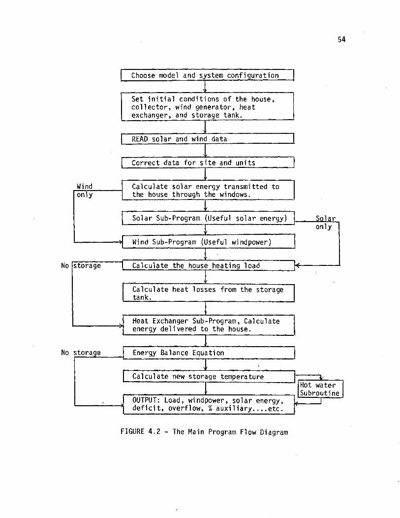
Choose model and system configuration 1

I

+ I READ so l a r and wind data I I 4

I Correct data f o r s i t e and units 1

Calculate s o l a r energy transmitted t o 1-1 the house through the windows. I

Solar Sub- Program (Useful s o l a r energy) Solar I only I

I Wind Sub-program (Useful wi ndpower) I I

1 [storage I Calculate the house heat ins load

4 - Calculate heat losses from the storage tank.

I

Energy Balance Equation 1 I

6

I Calculate new s torage temperature 3. 1 Itlot water I

' Heat Exchanger Sub-program, Calculate enerqy de l i vered t o the house.

FIGURE 4 .2 - The Main Program Flow Diagram

b . ISubroutine 1 ' OUTPUT: Load, wi ndpower , s o l a r energy,

d e f i c i t , overflow, % aux i l i a ry .... e t c . s+-J

diameter and height , the storage tank size, and o ther important parameters.

Next, the program reads the data, from the data sub-program described l a t e r ,

which i s based on hour l y measurements o f s o l a r i nso la t i on , c loud covers,

a i r temperature, wind v e l o c i t y and d i r e c t i o n . The program w i 11 c o r r e c t

the g iven data f o r s i t e and u n i t di f ferences i f necessary. The program

ca lcu la tes , us ing the s o l a r sub-program, the hour l y p o s i t i o n o f t h e sun

w i t h respect t o the house. Then, i t determines the amount o f s o l a r energy

t ransmi t ted through the windows i n t o the house. The energy a v a i l a b l e

from the wind generator and/or the s o l a r c o l l e c t o r i s determined by using

the proper sub-program. A d e t a i l e d d e s c r i p t i o n o f the sub-program i s g iven

i n the f o l l o w i n g sect ions. The house heating load i s determined, us ing the

load sub-program, by c a l c u l a t i n g separate ly the heat losses due t o i n -

f i l t r a t i o n and the convect ive heat losses from the house minus the s o l a r

energy t ransmi t ted t o the house through the windows. The program a l s o

ca lcu la tes the heat losses from the storage tank i n t o the basement. The

energy de l i ve red by the baseboard heat exchangers i s determined by using

the heat exchanger sub-program. The main program performs an energy balance

o f the whole system which inc ludes the energy a v a i l a b l e from the wind and/

o r the sun, the energy de l i ve red by the baseboard. heat exchangers, and the

change i n the amount o f energy s tored i n the storage tank ( fo r models w i t h

storage). As a r e s u l t of the energy balance the program ca lcu la tes a new

storage temperature. If the new storage temperature i s below the lower

l i m i t (70°F) t h e computer program w i l l s e t t h e storage temperature equal

t o t h e lower l i m i t and c a l c u l a t e the system energy d e f i c i t ( t he d e f i c i t i s

equal t o the a u x i l i a r y heat t h a t t h e house uses du r ing t h a t hour) . I f the

s to rage tempera tu re exceeds t h e upper 1 i l n i t (1 90°F) t h e program w i l l s e t

the tempera tu re equal t o t h e upper l i m i t and show an o v e r f l o w o f energy

(which means t h a t t h e r e i s more energy a v a i l a b l e than t h e s to rage hea t

c a p a c i t y and t h e h e a t i n g l o a d d u r i n g t h a t hou r ) .

I f domest ic h o t wa te r i s t o be d e l i v e r e d by t h e system t o t h e house,

t h e computer program w i l l f o l l o w t h e same procedure, g i v i n g p r i o r i t y t o

t h e h e a t i n g load , t hen t o t h e domest ic h o t wa te r demands. The main program

c a l c u l a t e s , us i ng t h e domest ic h o t wa te r sub- rou t ine , t h e energy p rov i ded i n

t h e form of domest ic h o t wa te r . The program a l s o r e c a l c u l a t e s t h e new

s to rage tempera tu re and s e t s t h e i n i t i a l c o n d i t i o n s o f t h e system f o r t h e

n e x t hour .

The program p r i n t s o u t h o u r l y , d a i l y , month ly , and/or y e a r l y

r e s u l t s o f t h e systeni performance.

4.2 The Data Sub-program

The da ta sub-program c o n s i s t s of s i x da ta banks, F i g u r e 4.3. Each

bank i n c l u d e s a p e r i o d o f two months s t a r t i n g w i t h September. A da ta bank

c o n s i s t s o f a number of l i n e s equal t o t h e number of hours i n t h e two

months pe r i od . Each l i n e has f i v e da ta p o i n t s t h a t a r e en te red i n t h e

f o l l o w i n g o r d e r : t h e s o l a r i n s o l a t i o n (SOL) on a s u r f a c e t i l t e d 60" f rom

t h e h o r i z o n t a l , c l oud cove r (CC), w ind v e l o c i t y ( V ) , a i r tempera tu re (TA),

and t h e w ind d i r e c t i o n (WD). The da ta banks a r e r ead one a t a t ime and

s t o r e d i n 'an a r r a y of t h e form (NHR,NDAY) , where NHR rep resen t s t h e hour

o f t h e day and NDAY r ep resen t s t h e day of t h e two months pe r i od .

1 READ SOLAR AND WIND HOURLY DATA I 1 SOL. CC, V . TA, WD. I

T

DATA BANK1 , SEPTEMBER AND OCTOBER 1

DATA BANK3, JANUARY AND FEBRUARY

DATA BANK5, MAY AND JUNE IC

1 DATA BANK6, JULY AND AUGUST I *

A CORRECT WIND DATA FOR U N I T S AND HEIGHT 1 I I CORRECT SOLAR DATA FOR INCIDENCE ANGLES 1 I

4

I M A I N PROGRAM CALCULATIONS 1 1

FIGURE 4.3 - F l o w D i a g r a m of t h e D a t a S u b - p r o g r a m

4.3 The Wind Sub-program

F i g u r e 4.4 shows a f l o w d iagram o f t h e wind gene ra to r sub-program.

The program s t a r t s by c o r r e c t i n g t h e g i ven da ta f o r u n i t s and h e i g h t .

To c o r r e c t f o r h e i g h t t h e w ind v e l o c i t y i s m u l t i p l i e d by a c o r r e c t i o n

f a c t o r (COF) which wi 11 g i v e t h e wind v e l o c i t y a t t h e wind gene ra to r h e i g h t . *

A lso, s i n c e t h e o u t s i d e hea t t r a n s f e r c o e f f i c i e n t o f t h e house w a l l s i s a

f u n c t i o n o f t he wind v e l o c i t y , t h e sub-program c a l c u l a t e s t h e wind v e l o c i t y

a t t h e house h e i g h t by m u l t i p l y i n g t h e v e l o c i t y w i t h a c o r r e c t i o n

c o e f f i c i e n t (COH), t h e two c o r r e c t i o n f a c t o r s COF and COH a r e determined

by u s i n g He l lman 's r e l a t i o n g i v e n i n Chapter 3. Then, u s i n g t h e cu rve

f i t t e d equa t i ons o f t h e gene ra to r power o u t p u t versus wind v e l o c i t y , t h e

sub-program c a l c u l a t e s , f o r a g i ven b lade d iamete r , t h e u s e f u l windpower

o u t p u t a v a i l a b l e t o t h e system.

4.4 S o l a r Sub-program

The s o l a r sub-program, F i g u r e 4.5, opera tes o n l y between t h e hours o f

s u n r i s e and sunset . The sub-program c a l c u l a t e s t h e s o l a r energy t r a n s m i t t e d

th rough t h e windows i n t o t h e house and t h e u s e f u l s o l a r energy c o l l e c t e d

by t h e f l a t - p l a t e c o l l e c t o r s . Th i s sub-program s t a r t s w i t h t h e f o l l o w i n g

i n p u t : t h e c o l l e c t o r s i z e , number o f g l az i ngs , t i 1 t and azimuth angles,

t h e s i t e l o n g i t u d e , and l a t i t u d e , t h e a i r tempera tu re and w ind speed, t h e

w a l l ' s az imuthang le , t h e i n i t i a l temperatures o f t h e c o l l e c t o r and t h e

wo rk i ng f l u i d . The sub-program c a l c u l a t e s : t h e s o l a r i n c i d e n c e ang le on

a l l ve r t i ca -1 su r f aces ( s i n c e a l l t h e windows and t h e c o l l e c t o r a r e v e r t i c a l )

and t h e c o r r e c t i o n s of t h e s o l a r i n s o l a t i o n s f o r a v e r t i c a l su r face . If

t h e model t e s t e d i n c l u d e s o n l y a wind gene ra to r t h e sub-program c a l c u l a t e s

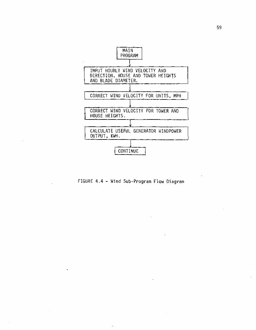
PROGRAM w INPUT HOURLY WIND VELOCITY AND D IRECTION, HOUSE AND TOWER HEIGHTS AND BLADE DIAMETER.

. . I CORRECT WIND VELOCITY FOR UNITS , MPH I I 4

CORRECT WIND VELOCITY FOR TOWER AND HOUSE HEIGHTS.

I i J,

CALCULATE USEFUL GENERATOR WINDPOWER OUTPUT, KWH.

I

FIGURE 4.4 - Wind S u b - p r o g r a m F l o w D i a g r a m

I n p u t : Hou r l y weather da ta , s v l a r i n s o l a t i o n , c l oud cover , c o l 1 e c t o r area, and o r i e n t a t i o n .

I I yes

r

I Energy absorbed by t h e house th rough t h e windows = 0.0 1 7

C a l c u l a t e d i r e c t and d i f f u s e d i n s o l a t i o n on t h e c o l l e c t o r , absorbed s o l a r energy by t h e c o l l e c t o r , hea t losses from t h e c o l l e c t o r .

L 1 L

I f t h e c o l l e c t o r l osses = Absorbed energy 1 I Yes

C o l l e c t o r ternp. = Prev ious hour temp. I :- I 1 C o l l e c t o r losses > Absorbed energy 1

v

[ A d j u s t new c o l l e c t o r temperature.

C o l l e c t o r e f f i c i e n c y = 0.0

I

I CONTINUE I

>

FIGURE 4.5 - So la r Sub-program B lock Diagram

C a l c u l a t e use fu l energy t r a n s f e r e d t o t h e work ing f l u i d , new c o l l e c t o r temperature, and t h e e f f i c i e n c y o f t h e c o l l e c t o r .

the so l a r energy gain through the windows and deletes the r e s t of the

sub-program. If the model includes a solar co l lec tor system then the

sub-program continues t o ca lcu la te : the co l lec tor overall heat t ransfer

coef f ic ien t , the col lector heat losses , the net (useful ) energy collected,

the eff ic iency of the co l lec tor , and the new col lec tor temperature. I f

the useful energy collected i s l e s s than or equal t o zero then the sub-

program s e t s the efficiency of the co l lec tor equal t o zero and calculates

the new col lec tor temperature.

4.5 The Load Sub-program

Figure 4.6 represents the flow diagram of the load sub-program, the

load calculations a re based on hourly weather data t ha t include ambient

a i r temperature, and wind velocity and d i rec t ion . This sub-program calculates

the model house heating load by determining separately the convective heat

losses from the windows, walls, doors, ce i l ing , f l o o r , and the i n f i l t r a t i o n

heat losses from the f i r s t f loor . I f the average home heating load i s t o

be determined, the sub-program performs the previous calculat ions . I t then

skips the f loor heat losses and adds the convective heat losses from the

basement walls, door, f loor and the basement i n f i l t r a t i o n losses. Since

so l a r energy i s transmitted through the house windows the sub-program

calculates the house net heating load by subtracting the so l a r energy

coming through the windows (as determined from the so la r subprogram) from

the to ta l heating 1 oad.

4.6 The Heat Exchanger Sub-program

This sub-program, Figure 4.7, covers two types of baseboard heater

systems. The f i r s t type consis ts of e l e c t r i c baseboard heaters tha t a re

[ Calculate windows l o s se s , N.W.S.&E. I 1 -

( Calculate walls losses . I

4. [ Calculate doors losses . I

I 4,

I Calculate c e i l i n g losses . 1 I

J . Calculate f i r s t f loor i n f i l t r a t i o n losses . (

I

4, I f "Average" house load. No

I

& I Calculate basement wall losses . I

4; Calculate basement f l oo r losses .

I 1 4,

Calculate basement windows and doors 1 I l o s ses . I I . ,'

Calcul a t e basement i n f i 1 t r a t i on losses . -. I

I Total "Average" house losses . I I .I.

I Heating load = Total house losses . I

Net heating load = Total - (Energy through windows)

(CONTINUE I FIGURE 4.6 - Flow Diagram of the Heating

Load Sub-program

r-! If t h e system has no s to rage .

Yes 1

Heat d e l i v e r e d = A v a i l a b l e energy i n s t o r a g e t a n k . I--

C a l c u l a t e h e a t d e l i v e r e d by t h e e l e c t r i c baseboard H.X.

C a l c u l a t e h e a t d e l i vered u s i n g t h e h e a t exchanger s p e c i f i c a t i o n s .

I

-

J. Check H.X. e x i t t empera tu re and keep q r e a t e r t h a n room temp.

Usefu l energy = Heat d e l i v e r e d .

1

FIGURE 4.7 - The Flow Diagram o f t h e H.X. Sub-program

o n l y used i n system models w i t h no s to rage (Model 1 ) . T h i s sub-program

performs h o u r l y energy balances between t h e h e a t i n g l o a d and t h e windpower

a v a i l a b l e f rom the wind genera to r . It has t h e f o l l o w i n g t h r e e p r e d i c t e d -

outcomes:

- t h e load i s g r e a t e r t han t h e windpower. The system i s i n

d e f i c i t and t h e a u x i l i a r y hea t i s sw i tched on.

- t h e l o a d i s equal t o t h e windpower. The system s u p p l i e s a l l

t h e load .

- t h e l oad i s l e s s t han t h e windpower. F o r t h i s case, t h e system

s u p p l i e s t h e h e a t i n g l o a d and ove r f l ows t h e rat ( t h i s e x t r a

energy c o u l d be used f o r domest ic h o t wa te r h e a t i n g ) .

The second t ype i s a conven t iona l h o t water baseboard h e a t i n g system

( w i t h an o p t i o n o f f i n i t e o r i n f i n i t e s i z e d hea t exchangers). The sub-

program c a l c u l a t e s t h e energy d e l i vered by t h e hea te rs as a f u n c t i o n o f

t h e s to rage temperature ( i n 1 e t temperature t o hea te rs ) .

4.7 The Domestic Hot Water (D.H.W.) Subrou t ine

The D.H.W. sub rou t i ne , F i g u r e 4.8, c a l c u l a t e s t h e house D. H.W. energy

requ i rement and t h e p o r t i o n o f t h a t energy supp l i ed by t h e wind and s o l a r

systems. The da ta i n p u t t o t h e sub rou t i ne i nc l udes t h e h o u r l y consumption

o f h o t water , t h e s to rage temperature (TS), and t h e des i r ed upper and lower

D.H. W. temperatures (THWU & THWL r e s p e c t i v e l y ) . If t h e s to rage temperature

i s l e s s than THWL, the s to rage tank a c t s as a p re -hea te r and t h e a u x i l i a r y

D.H.W. fu rnace wi 11 h e a t water up t o THWU. The sub rou t i ne c a l c u l a t e s t h e

a u x i l i a r y energy used and t h e energy d e l i v e r e d by t h e s to rage tank . If

t h e s to rage ternperature i s g r e a t e r than TtIWUy then c o l d water f rom t h e main

.b

S p e c i f y upper, lower and d e s i r e d temp- e r a t u r e s o f t h e domest ic h o t water .

w I

- INPUT: Hour, day, month, s to rage temp. and s i ze .

.L

I READ h o u r l y D.H.W. demand i n ga l l ons . I I

L

C

I C a l c u l a t e energy r e q u i r e d f o r D.H.W. 1 1

I

.L I f energy a v a i l a b l e i n s t roage.

1 Yes 1

I Energy used= D.H.W. energy requ i rement D e f i c i t = 0.0

I 1 C a l c u l a t e a u x i l i a r y energy needed. & D e f i c i t = a u x i l i a r y energy needed.

r .L Energy used = D.H.W. energy r e q u i r e d

- A u x i l i a r y needed 1

. I C a l c u l a t e new s to rage temperature.

I

CONTINUE c 3 FIGURE 4.8 - The D.H.W. Subrou t ine F low Diagram

i s mixed w i t h the h o t water f rom storage u n t i l t h e temperature o f the

m i x t u r e i s equal t o THWU, and the energy de l i ve red by the system i s

equal t o t h e D.H.W. energy demand. I f the storage temperature i s between

THWU and THWL, then t h e storage ho t water i s d e l i v e r e d d i r e c t l y t o t h e

house ( the energy d e l i v e r e d by the system i s equal t o t he D.H.W. energy

demand). A f t e r each hou r ' s c a l c u l a t i o n , t he subrout ine c a l c u l a t e s t h e

new storage temperature.

C H A P T E R 5

SYSTEM PERFORMANCE AND ANALYTICAL RESULTS

This chapter inc ludes the a n a l y t i c a l r e s u l t s based on the system

performance o f a l l the models described i n the previous Chapters. A l l

systems a re tested f o r both the "Average" and "Model" homes (mainta in ing

i n s i d e temperature a t 68°F) by vary ing key system parameters such as:

1 ) w i nd generator b l ade diameter

2) wind generator tower he igh t

3 ) water storage tank s i z e

4) t h e heat d e l i very system s i z e

5 ) t he s o l a r c o l l e c t o r s i z e

5.1 General Backqround

The house heat ing requ i renients and wind energy are determined by

using the 1971 weather data (ambient temperature, wind v e l o c i t y and '

d i r e c t i o n ) from Har t fo rd , Connecticut. The s o l a r energy i s obtained from

the 1958 Blue H i l l s , Massachusetts s o l a r data ( s o l a r i n s o l a t i o n and c1,oud I

cover). These two s i t e s were chosen as representat ives o f the weather

cond i t ions i n the Northeastern p a r t o f the Uni ted States. Other computer

runs w i l l be made w i t h l i m i t e d data a v a i l a b l e from other s i t e s and the

r e s u l t s of these runs w i l l be g iven a t t h e end o f t h i s chapter.

Table 5.1 gives a monthly summary o f the heat ing load of both the

"Average" and "Model" homes based on the Har t fo rd weather data. Also

shown i n Table 5.2 i s the monthly average t o t a l r a d i a t i o n per day f a l l i n g

on a v e r t i c a l sur face and on a surface t i l t e d 60" from the ho r i zon ta l . (27)

Also, based on a d e t a i l e d computer ana lys is o f standard wind generator

and aerodynamic prac t ice , (25) F igure 5.1 represents the wind generator n e t

Month

September

October

November

December

January

February

March

A p r i 1

T o t a l l o a d f o r h e a t i n g season

"Model I' House (no basement)

1589.7

854.6

16624.9 kWhr

"Average" House (model w i t h basement)

1632.8

31 969.5 kWhr

TABLE 5.1 - R e s i d e n t i a l Hea t ing Requirements f o r (6600 Degree Day C l imate ) o f Ha r t f o rd , Connec t i cu t

January

February

March

Apr i 1

May

June

J u l y

August

September

October

November

60" T i l t e d Surface

V e r t i c a l Surface

Deceniber

TABLE 5.2 - Average Monthly Solar Inso la t i on , 8tu/ f tZ/month

. . 0

. . 10 I S 20 25 30 35

WIND SPEED, MPH

F I G U R E 5.1 - The Wind Generator Performance Curves.

power output, for different blade diameters, as a function of the w-ind

velocity.

Figure 5.2 ref lects the importance of the wind generator parameters,

blade diameter and tower height and the i r effect on €he maximum yearly

power output. I t i s important to notice that the blade diameter has a

greater impact on the power input t h a n the tower height. For comparison,

th is - f igures also shows the yearly maximum energy input of a 200 square

foot vertical solar collector. The heating requirements of both the "Model"

and "Average" homes are added to Figure 5.2 t o i l l u s t r a t e the magnitude of

the maximuni wind and solar energy inputs in relation to the yearly heating

load of each residence. From the figure one can see that a small wind

generator or a 200 square foot solar collector could "in principle"

supply the heating requirement of the model home b u t , as a resul t of the

discrepancy in time between the energy avai labi 1 i ty and consumption (see

Figure 5.3) these systems cannot supply a l l the heating load.

Figure 5.3 represents typical monthly values of the "Averagen home

energy requirements and the energy input of representative wind and solar

systems. The windpower output shown in the figure i s based on a 32.5

foot blade diameter wind generator placed on an 80 foot high tower and

the solar energy input i s given for a 200 square foot f l a t plate solar

collector mounted vertically on the south wall of the house. Due t o the

interaction between the system components and various loss terms the amount

of solar and wind energy the system del ivers to the house i s less than

the energy inputs shown in th is figure. In order to determine the exact

amount of useful energy the system contributes, an hour-by-hour analysis

-

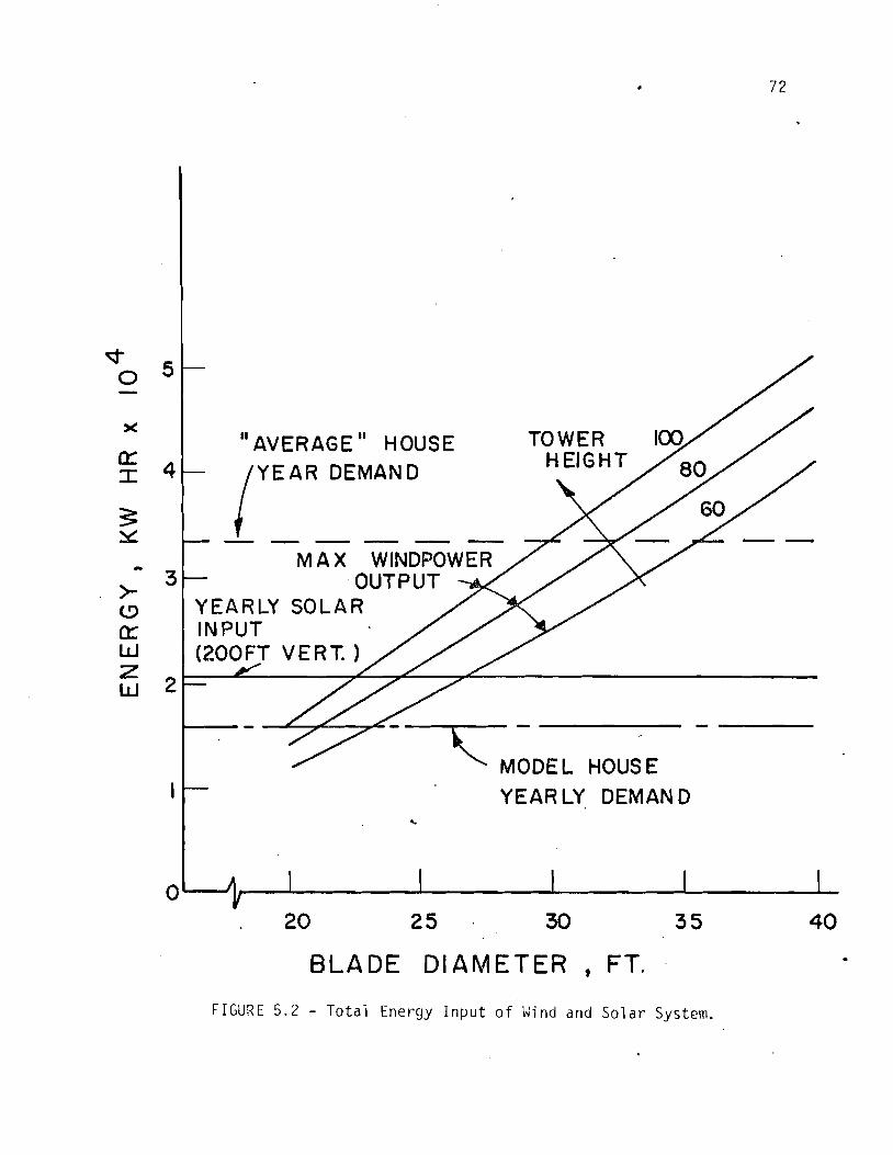
"AVERAGE" HOUSE Y E A R D E M A N D

- M A X WINDPOWER

YEARLY SOLAR

--

- O D E L HOUSE

YEARLY DEMAN D 5

BLADE DIAMETER , FT. -

F I G U R E 5 . 2 - Total Energy I n p u t of Wind and So la r System.

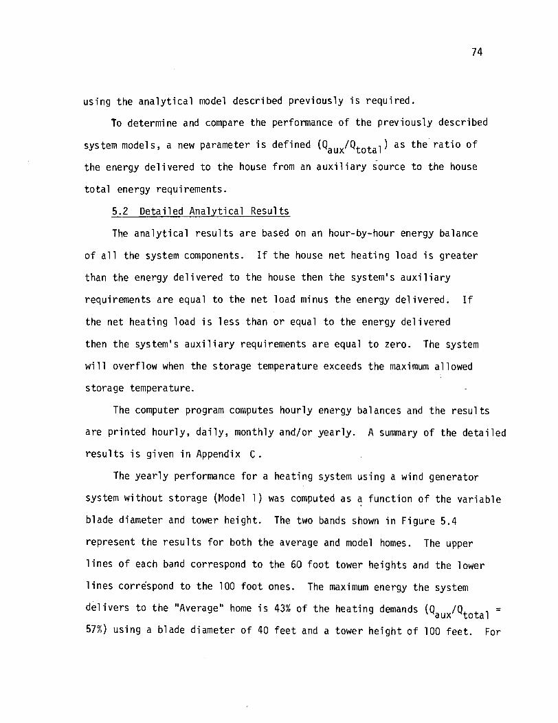
us ing the a n a l y t i c a l model descr ibed p rev ious l y i s requ i red .

To determine and compare the performance o f t h e p rev ious l y descr ibed

system models, a new parameter i s def ined (Qaux/Qtotal ) as t h e r a t i o o f

t he energy de l i vered t o the house from an aux i 1 i ary source t o the house

t o t a l energy requirements.

5.2 De ta i l ed A n a l y t i c a l Resul t s

The a n a l y t i c a l r e s u l t s a re based on an hour-by-hour energy balance

of a l l the system components. I f t h e house n e t hea t i ng l oad i s g rea te r

than the energy de l i ve red t o t h e house then the system's a u x i l i a r y

requirements a re equal t o the n e t load minus t h e energy de l i ve red . I f

the n e t heat ing load i s l e s s than o r equal t o the energy del i ve red

then t h e system's a u x i l i a r y requirements a r e equal t o zero. The system

w i l l over f low when the storage temperature exceeds the maximum al lowed

storage temperature.

The computer program co~liputes hou r l y energy balances and the r e s u l t s

a re p r i n t e d hour ly , d a i l y , monthly and/or y e a r l y . A summary o f t he d e t a i l e d

r e s u l t s i s g iven i n Appendix C . The y e a r l y performance f o r a heat ing system us ing a wind generator

system w i thou t s torage (Model 1 ) was computed as a func t i on o f t he v a r i a b l e

b lade diameter and tower he igh t . The two bands shown i n F igu re 5.4

represent t h e r e s u l t s f o r bo th t h e average and model homes. The upper

l i n e s o f each band correspond t o the 60 f o o t tower he igh ts and the lower

l i n e s correspond t o t h e 100 foo t ones. The maximum energy t h e system

d e l i v e r s t o t h e "Average" home i s 43% of t h e heat ing demands (Qaux/Qtotal - -

57%) us ing a blade diameter of 40 fee t and a tower h e i g h t of 100 f e e t . For

NO ENERGY STORAGE SYSTEM TOWER HEIGHTS : 60 to 100 ft.

"AVERAGE " RESIDENCE (MODEL W/BASEMENT)

I MODEL HOME?

BLADE DIAMETER, FT.

FIGURE 5 . 4 - Performance o f the Wind wi th no Storage System - Model 1 .

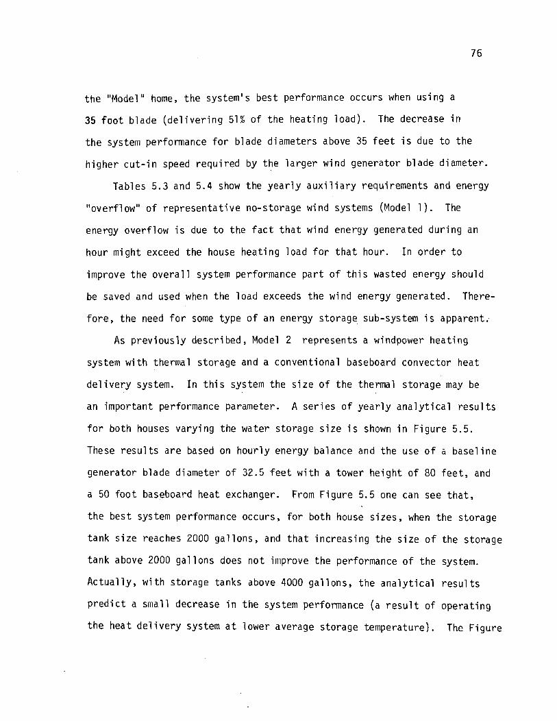
t h e "Model" home, t h e system's b e s t performance occurs when us ing a

35 f o o t b l ade ( d e l i v e r i n g 51% o f t h e hea t i ng l o a d ) . The decrease i n

t h e sys te~ i i performance f o r b lade d iameters above 35 f e e t i s due t o t h e

h i g h e r c u t - i n speed r e q u i red by t h e l a r g e r wind genera to r b l ade d iameter .

Tables 5.3 and 5.4 show t h e y e a r l y a u x i l i a r y requ i rements and energy

"ove r f l ow" o f r e p r e s e n t a t i v e no-s to rage wind systems (Model 1 ) . The

energy o v e r f l o w i s due t o t h e f a c t t h a t wind energy generated d u r i n g an

hour m i g h t exceed t h e house h e a t i n g l o a d f o r t h a t hour. I n o r d e r t o

improve t h e o v e r a l l system performance p a r t o f t h i s wasted energy should

be saved and used when t he l o a d exceeds t h e wind energy generated. There-

f o r e , t h e need f o r some t ype of an energy s to rage sub-system i s apparent .

As p r e v i o u s l y descr ibed , Model 2 r ep resen ts a windpower h e a t i n g

system w i t h thermal s to rage and a convent iona l baseboard convec to r hea t

d e l i v e r y system. I n t h i s system t h e s i z e o f t h e thermal s to rage may be

an impo r tan t performance parameter. A s e r i e s of y e a r l y a n a l y t i c a l r e s u l t s

f o r b o t h houses v a r y i n g t h e water s to rage s i z e i s shown i n F i g u r e 5.5.

These r e s u l t s a r e based on h o u r l y energy ba lance and t h e use o f a b a s e l i n e

genera to r b lade d iameter of 32.5 f e e t w i t h a tower h e i g h t o f 80 f e e t , and

a 50 f o o t baseboard hea t exchanger. From F i g u r e 5.5 one can see t h a t ,

t h e b e s t system performance occurs, f o r b o t h house s i zes , when t h e s to rage

tank s i z e reaches 2000 g a l l o n s , and t h a t i n c r e a s i n g t h e s i z e of t h e s to rage

t ank above 2000 g a l l o n s does n o t improve t h e performance of t h e system.

A c t u a l l y , w i t h s to rage tanks above 4000 ga l l ons , t h e a n a l y t i c a l r e s u l t s

p r e d i c t a sma l l decrease i n t h e system performance (a r e s u l t o f o p e r a t i n g

t h e h e a t d e l i v e r y system a t l owe r average s to rage temperature) . The F i g u r e

D- HT DEF OVRFL- F t . F t . kl.lh/yr kWh/yr

TABLE 5.3 - Representat ive Energy "over f low" o f

No-storage Wind Systems, ("Model "

house l oad ) .

D HT DEF OVRFL F t . -- F t . kWh/yr k Whlyr --

TABLE 5.4 - Rep resen ta t i ve Energy " o v e r f 1 ow" o f No-storage

Wind Syste~i is, ( ' 'Average" house 1 oad) .

Qoux

TOVJER tiElG HT = 8 0 FT.

BLADE DlPlMETER = 32.5 FT.

"AVERAGE" HOME ( W / BASEMENT)

MODEL HOME

( NO BASEMENT 1

I I I

STORAGE S I Z E , GALLONS F I G U R E 5.5 - Wind System Performance as a Func t ion of Storage Tank Size.

shows t h a t t h i s systen~, w i t h 2000 g a l l o n s s to rage , p rov ides a l l t h e

h e a t i n g requ i re~ l l en t s o f t h e "Model" house and over 70% o f t h e "Average"

house hea t i ng demands.

A lso, f o r t h e Model 2 systeni, a number o f a n a l y t i c a l runs va ry i ng

the s i z e and t ype o f t h e hea t d e l i v e r y systeni was performed (Tab le 5 .5 ) ,

r e v e a l i n g an i n s e n s i t i v i t y t o Qaux/Qtotal once a minimun~ (and p r a c t i c a l )

hea t exchanger s i z e was se lec ted . The t a b l e g i ves a sample y e a r l y

performance o f a nuniber o f wind systems w i t h a v a r i a b l e l e n g t h baseboard

hea t exchanger (50 ft., 100 f t . , and i n f i n i t e ) o p e r a t i n g w i t h t h e "Average"

house h e a t i n g load , a v a r i a b l e b lade d iameter , a cons tan t s t o rage s i z e

(1000 g a l l o n s ) , and tower h e i g h t (80 f t . ) .

F i g u r e 5.6 represen ts t he performance curves o f t h e wind genera to r

system w i t h s to rage (Model 2 ) as a f u n c t i o n o f t h e wind genera to r

parameters, t h e b l ade d iameter and t h e tower he igh t . Based on t h e

p rev ious r e s u l t s , t h e s i z e o f t h e s to rage tank i s kep t cons tan t a t 2000

g a l l o n s and 50 f e e t hea t exchanger w h i l e v a r y i n g e i t h e r t he b lade d iameter

(20-40 f e e t ) o r t h e tower h e i g h t (60-100 f e e t ) . The upper l i n e s o f each

band correspond t o t h e 60 f o o t tower h e i g h t s and t h e lower l i n e s correspond

t o the 100 f o o t ones. The f i g u r e s shows t h a t t h i s system c o u l d supp ly over

80 pe rcen t o f the "Average" house hea t i ng demands, u s i n g a 40 f o o t b l ade

d iameter . However, u s i n g t h e b a s e l i n e 32.5 f o o t d iameter wind genera to r

a t a 60 f o o t tower t he system would be ab le t o supp ly a l l t h e h e a t i n g demands

o f t h e "Model" home. I n comparing t h i s system w i t h t h e no s to rage one

(F igu re 5.4) i t can be seen t h a t t h i s t y p e o f system rep resen ts a s i g n i f i -

c a n t source o f energy f o r home hea t i ng .

D H. X. Length C+ Qaux'Qtotal

TABLE 5.5 - E f f e c t of t h e S i ze o f t h e Heat D e l i v e r y

System on t h e System Performance, Model 2.

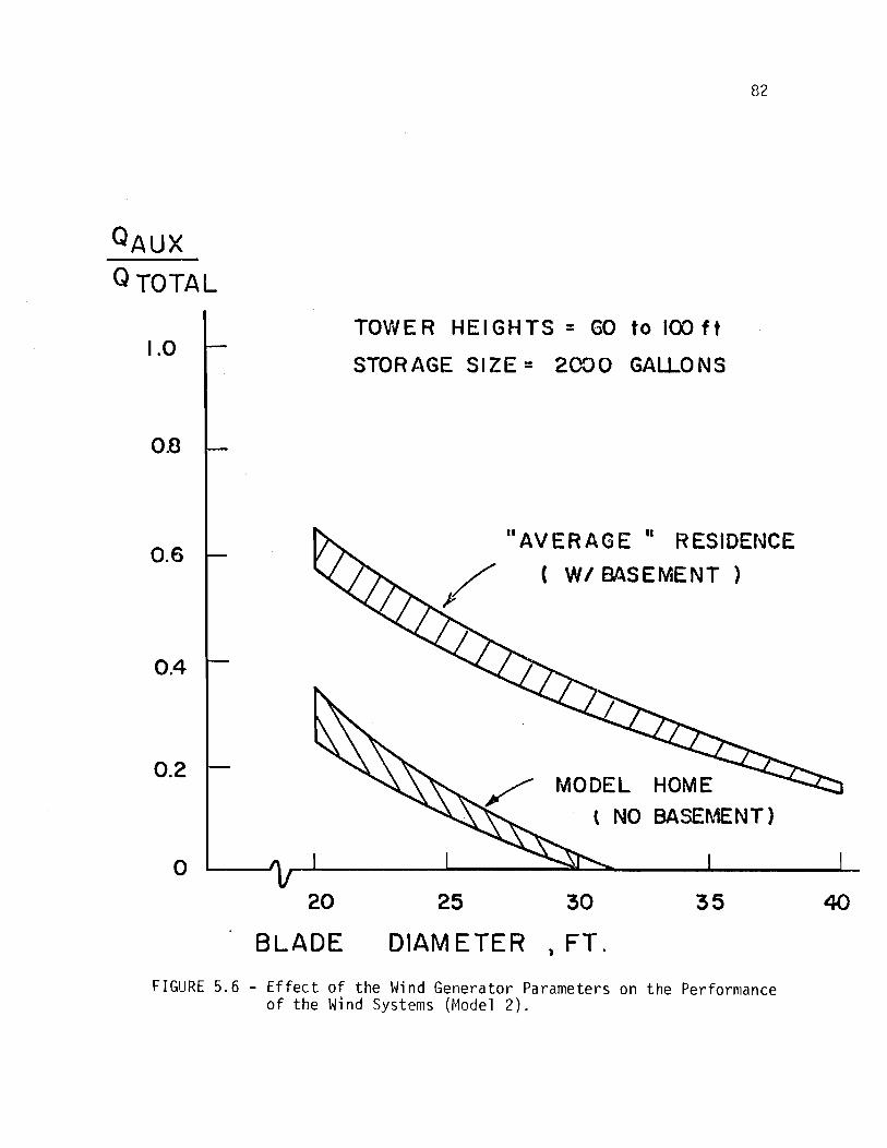
TOWER HEIGHTS = GO to I00 f t

STORAGE SIZE = 2 0 0 GALLONS

" A V E R A G E " RESIDEIJCE

MODEL HOME ( NO BASEMENT)

BLADE DIAMETER , FT.

FIGURE 5.6 - E f f e c t o f t he Wind Generator Parameters on t he Performance o f t h e Wind Systems (Model 2 ) .

S i m i l a r t o t he wind system, the per for~ i iance o f t he s o l a r syst,r l l~ i s f

d funct. iot i o f tho storage s i z c i ~ n d t t ie (Irca o f t t lc s o l ~ r . collector. r i l j i ~ r c s

formance o f 200 t o 600. ftL c o l l e c t o r area s o l a r systen~s, w i t h a 50 foot

heat exchaqger, as a f u n c t i o n o f t he storage tank s i ze . The curves i n

t h e f i g u r e s show l i t t l e s e n s i t i v i t y t o the storage s i z e when i t exceeds

2000 ga l lons . They a l s o show t h a t a s o l a r system w i t h 600 ftL c o l l e c t o r

and 2000 g a l l o n tank w i l l p rov ide 90 percent o f the heat ing requirement

o f t he "Model" home, b u t o n l y about 40 percent f o r t he "Average" home.

To determine the performance o f the s o l a r system as a f u n c t i o n o f

t he c o l l e c t o r s i z e the storage s i z e i s kept cons tant a t 2000 g a l l o n s and

the heat exchanger a t 50 f e e t w h i l e va ry ing t h e area o f t he c o l l e c t o r .

2 F igures 5.9 and 5.10 show t h a t the s o l a r system w i t h 800 ft c o l l e c t o r

w i l l p rov ide about 90 percent and 60 percent o f the y e a r l y hea t i ng requ i re -

ments o f t he "Model" and "Average" homes r e s p e c t i v e l y . The slopes o f the

curves i n both f i g u r e s s t a r t t o dewease r a p i d l y w i t h i nc reas ing c o l l e c t o r

s ize , due t o t h e f a c t t h a t t he e f f i c i e n c y of t h e c o l l e c t o r decreases w i t h

the increase o f t he i n l e t temperature t o t h e c o l l e c t o r .

2 The y e a r l y performance of a 200 f t c o l l e c t o r s o l a r system, a 32.5

f o o t blade diameter wind system (Model 2) and a combined s o l a r and wind

system (Model 3-A) a r e compared i n F igures 5.11 and 5.12 as a f u n c t i o n o f

t h e s i n g l e tank s to rage s i z e w i t h a 50 f o o t heat exchanger. As p r e v i o u s l y

2 shown i n F igu re 5.7, f o r t he "Model" house, a 200 ft c o l l e c t o r s o l a r system

i s very smal l and w i l l p rov ide o n l y about 60 percent o f the house heat ing

requirements, w h i l e t he wind o r t he combined s o l a r and wind system w i t h a

HEAT EXCHANGER = S o f t .

F I G U R E 5.7 - Solar Systern Performance - "flodel" House.

-

-

-

ACOL = 200 f t -

1.0

.80

.20 ACOL = 400 f t 2

ACOL = 6 0 0 f t 2 1

0 I I I I I 1

0 loo0 2000 m o 4000 5000

STORAGE SIZE, GALLONS

x 3 Q 0

.60 0 t- CY

.40

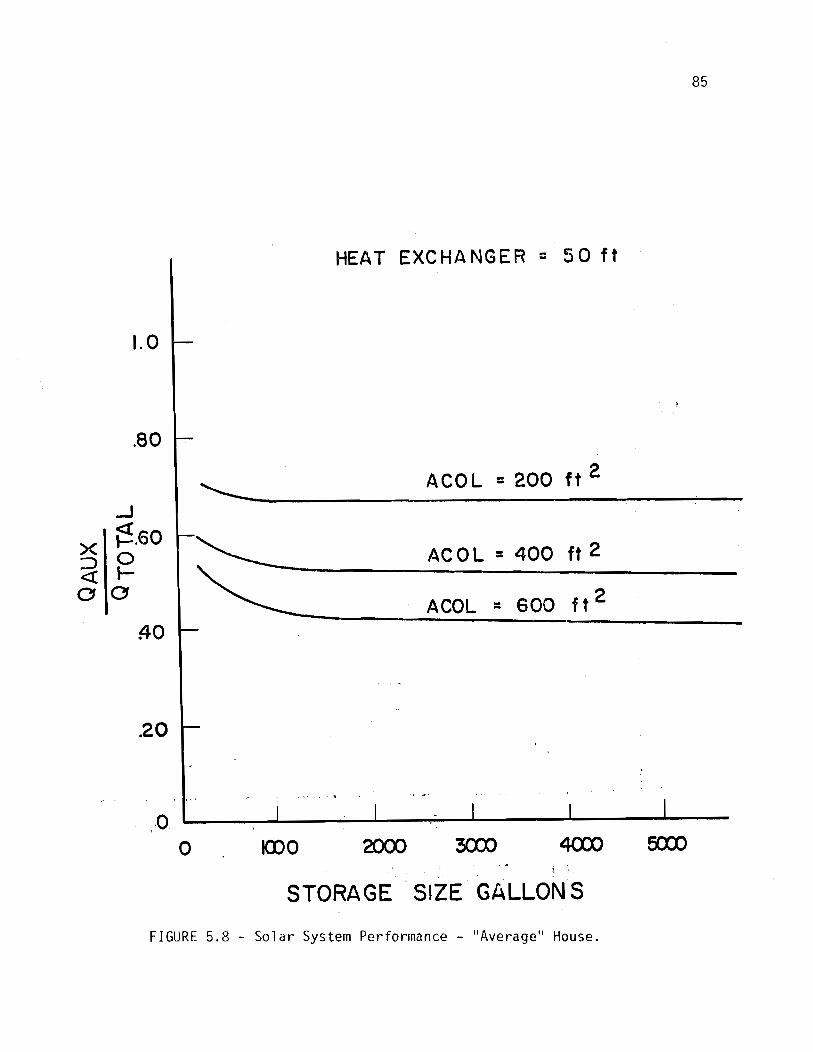
HEAT EXCHANGER = 5 0 f t

F I G U R E 5.8 - S o l a r System Per formance - "Average" House.

1.0

-80

J

X $60 3 0 a k 0 0

40

.20

0

-

-

A C O L = 200 f t

- ACOL = 400 f t 2

ACOL = 600 f t -

-

. . - 1 I

0 . mo 2000 3C00 4000 5000 I

STORAGE ' SlZE GALLONS

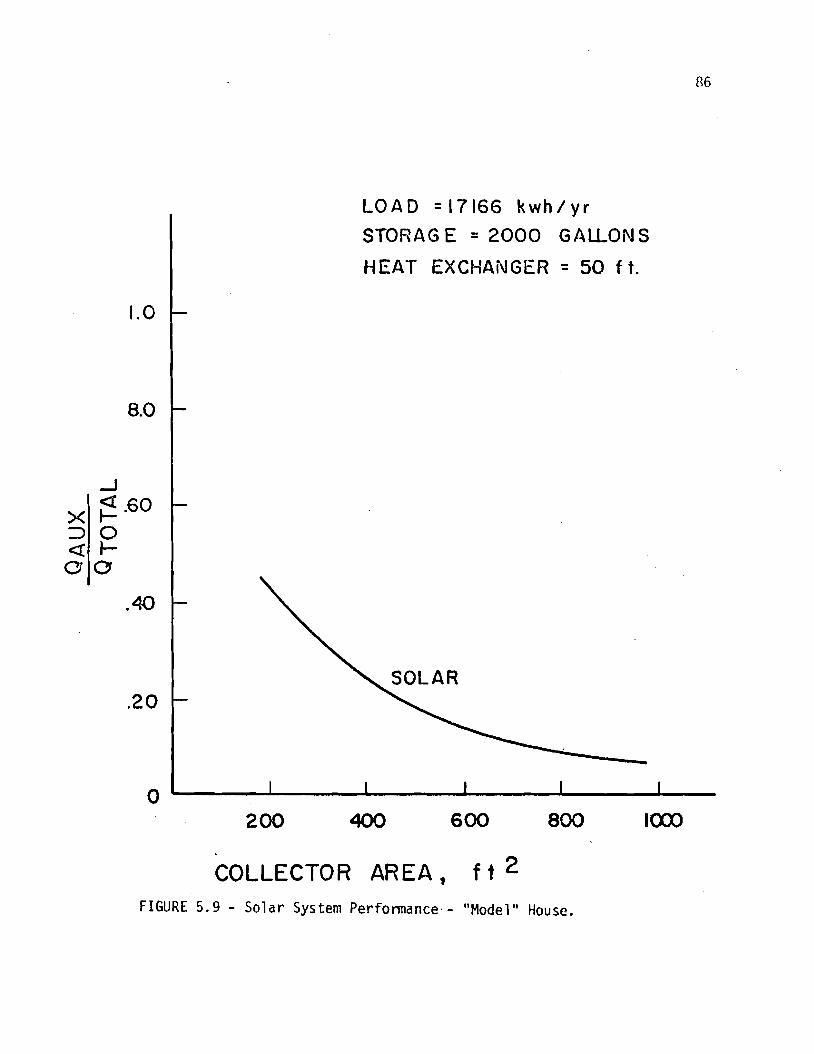
L O A D 47166 k w h / y r

STORAG E = 2000 GALLONS

HEAT EXCHANGER = 50 f t .

COLLECTOR AREA, f t FIGURE 5 . 9 - S o l a r System Performance - "Model" House.

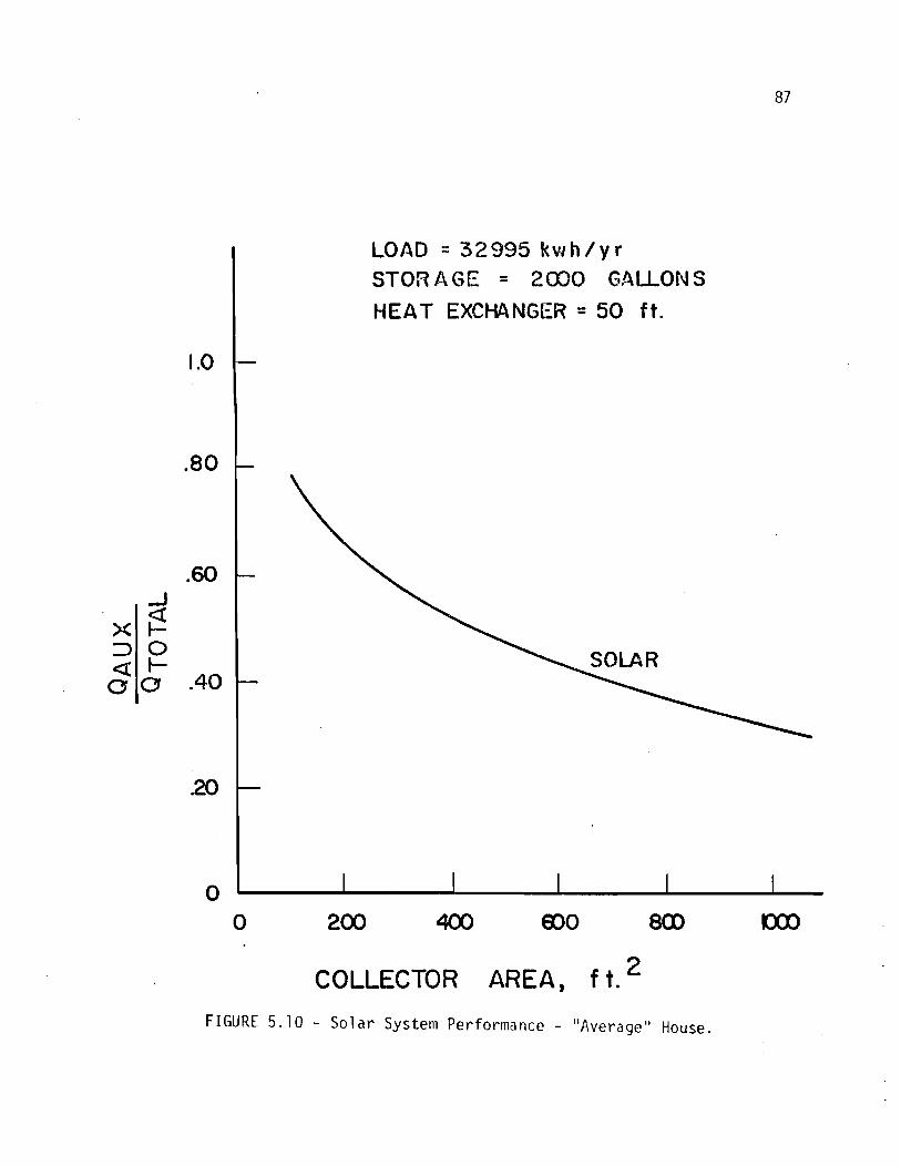
LOAD = 32995 k w h / y r S T O R A G E = 2030 GALLONS

HEAT EXCHANGER = 50 f t .

F I G U R E 5.10 - S o l a r Systeni Perforinance - "Average" House.

-

-

-

-

1

1.0

.80

.60 J

0 200 ($00 800 800 KXX)

COLLECTOR AREA, f t.

X 3

00

a t- o

4 0 - -

.20

0

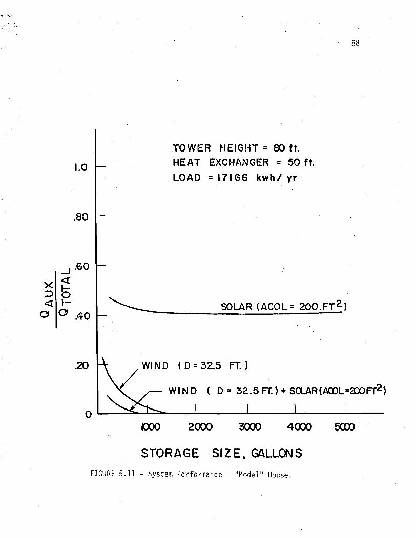
TOVJER WEIGHT = 80 ft. HEAT EXCHANGER = Soft . LOAD = I 7 1 6 6 kwh/ y r -

h/T ( D = 32.5 F K

WIND ( D = ~ ~ . ~ F ~ ~ + s u R ( A C X I L = ~ ~ ~ ~ )

STORAGE SIZE, GALLONS

FIGURE 5.11 - System P e r f o r ~ i i a n c e - "Model" House.

Q oux ~ -

Q total

I' A V E R A G E " HOUSE

- SOLAR ONLY ( 2 0 f t 2 COLLECTOR)

WIND CNLY ( 8 0 ft. TOWER 32.5 f t . D IA. DLA

S O L A R + WIND

. STORAGE S I Z E , G A L L O N S

F I G U R E 5 .12 - Sys teln Perforniance "Average" House.

s to rage s i z e l e s s than 1500 g a l l o n s w i l l p r o v i d e a l l t h e hea t i ng r e q u i r e -

ments o f t h e house. S i m i l a r l y , f o r the "Average" house, F i g u r e 5.12 shows

t h a t t h e s o l a r system w i l l p r o v i d e o n l y about 35 percen t , t h e wind system

about 75 percen t , and t he combined system 85 pe rcen t ' o f t h e h e a t i n g load.

'This f i g u r e a l s o shows t h a t , over a wide range o f s to rage tank s i zes , t h e

2 a d d i t i o n o f a 200 f t c o l l e c t o r o n l y inc reases i t s energy based performance

by about 10 percen t .

To f u r t h e r i n v e s t i g a t e t h e e f f e c t s o f c o l l e c t o r s i ze , F i g u r e 5.13

g i ves t h e performance curves of combined s o l a r and wind systems w i t h

v a r i a b l e c o l l e c t o r area as a f u n c t i o n o f t h e s to rage s i z e . The combined

systems cons idered used a 32.5 f t . b lade d iameter wind genera to r , an 8 0 f o o t

tower, a 50 f o o t hea t exchanger and 200, 300, 400 ft.' s o l a r c o l l e c t o r s .

The f i g u r e s show t h a t , f o r t h e "Average" house, i n c r e a s i n g t h e c o l l e c t o r

area by 100 ft.' w i l l improve t h e o v e r a l l system performance by 3-4 percen t .

For t he "Model" house, t h e system i s l e s s s e n s i t i v e t o t h e c o l l e c t o r area

s ince, as i t was shown e a r l i e r i n t h i s chap te r , w i t h modest s to rage s izes ,

t h e wind system a lone would p r o v i d e a l l t h e h e a t i n g requ i rements o f t h a t

house. F i g u r e 5.14 i s based on a s i m i l a r system w i t h t h e c o l l e c t o r area

cons tan t w h i l e v a r y i n g t h e b lade d iameter . T h i s f i g u r e s shows t h a t by

i n c r e a s i n g t h e b lade d iameter from 25 t o 32.5 ft. t h e system performance

inc reases by approx imate ly 15 percen t , w h i l e i n c r e a s i n g t h e d iameter f rom

32.5 t o 40 ft. r e s u l t s o n l y w i t h about a 5 pe rcen t i nc rease i n t h e o v e r a l l

system performance. The decreas ing e f f e c t i n performance o f t h e l a r g e r

s i zed wind genera to rs i s p r i m a r i l y due t o mismatch o f energy supp ly and

demand, r e s u l t i n g i n s i g n i f i c a n t energy over f low.

BLADE DIAf'AETEE = 32.5 f t TOWER HEIGHT = 80 f t .

HOUSE 32995 kw

ACOL

200 f t 3063

17166 ~ t u h / c , r

0 loo0 2000 3008 4000

. STORAGE SIZE , GALLONS

FIGURE 5.13 - So la r and Wind Systeni Performance.

AUX.

" A V E R A G E " HOUSE

TOWER HEIGHT = 80 FT. ACOL = 2 0 0 F T . ~

WIND 8r SOLAR

STORAGE S I Z E , GALLONS

F I G U R E 5.14 - Performance o f Combined Solar and Wind Systems.

A suliunary o f t h e y e a r l y energy performance on t h e "Average" house

of t h e combined s o l a r and wind systems (Model 3A) i s g i ven i n F igu res 5.15

2 t o 5.20. They i n c l u d e t h e e f f e c t s of c o l l e c t o r area (200 t o 600 ft. ) , tower

h e i g h t (40 t o 80 f t . ) and b lade d iameter (25 t o 40 ff. ) . These r e s u l t s

show t h a t by i n c r e a s i n g t h e s i z e of any one o f t h e t h r e e parameters

inc reases t h e o v e r a l l performance o f t h e system. However, t hey c o n s i s t e n t l y

i n d i c a t e t h a t t h e r a t e o f t h e performance inc rease , decreases w i t h

i n c r e a s i n g s i z e o f t h e parameter. Fo r example, from F igu re 5.18, i n c r e a s i n g

t h e tower h e i g h t f rom 40 t o 60 ft. inc reases t he o v e r a l l performance by

6 percen t , whi ' le t h e same i nc rease i n t h e he igh t , 60 t o 80 ft., r e s u l t s

i n o n l y a 3 pe rcen t i nc rease i n t h e system performance. One reason f o r

t h i s e f f e c t i s due t o t h e f a c t t h a t i n c r e a s i n g t h e s i z e o f one o f these

system components inc reases t h e amount of energy a v a i l a b l e t o t h e system

which causes an i nc rease i n t he i n l e t temperature o f t h e c o l l e c t o r ,

r educ ing t h e c o l l e c t o r e f f i c i e n c y . Another i s t h a t t h e y cause an i nc rease

i n t h e amount o f energy wasted (system o v e r f l o w ) due t o t i m e l a g s between

t h e house hea t i ng demands and t h e a v a i l a b l e energy.

A summary o f t h e expected performance o f t h e llMass s o l a r and wind

system us ing Models 2 and 3-A i s shown i n F igu re 5.21. The systems combine

2 a f l a t p l a t e s o l a r c o l l e c t o r (200 ft. ), a 32.5 ft. b lade d iameter wind

genera to r mounted on a 60 f t . tower , a 2000 g a l l o n s to rage tank, and a 50

f o o t baseboard hea t exchanger. Both t h e wind o n l y and t h e wind and s o l a r

systems a r e compared f o r t he "Model " and "Average" house (cor respond ing

t o t h e p r e s e n t system a t t h e U n i v e r s i t y o f Massachusetts, Amherst ( 3 3 ) )

Q TOTAL ,6

" A V E R A G E " HOUSE

HT = 4 0 FT. STORAGE = 2 0 0 0 GAL.

BLADE DIAMETE R , FT.

F I G U R E 5 . 1 5 - P e r f o r ~ l ~ a n c e o f Combined S o l a r arid Wind Systems.

TOTAL .6

" A V E R A G E " HOUSE HT = 60 FT. STORAGE= ~ O O O G A L .

ACOL

200 F T ~ 4 0 0 F T ~

BLADE DIAMETER , FT FIGURE 5.16 - Performance of Conibined So la r and Wind Systems.

TOTA L

" AVE RAGE " HOUSE

HT = 8 0 FI STORAGE = 2 0 0 0 G A L .

-

-

-

-

- ACO L

2 0 0 FT; 400 FT

I I I I I 6 0 0 F T ~

BLADE D.IAMETER, FT

FIGURE 5.17 - Performance o f Conibined S o l a r and Wind Systems.

AUX.

Q TOTAL .6

LOAD = 3 2 9 9 5 k W h

H .X . = 5 0 FT.

TAN K = 2 0 0 0 GA L. A C O L = 2 0 0 F T . ~

HT. - 40 FT. 60 FT. 80 FT.

BLADE DIAMETER - FT.

FIGURE 5.18 - Perforrnance o f Conibined S o l a r and Wind Systems.

1 .o

.8

.6 ' AlJ X .

TOTAL

4

.2

0

"AL/ERI(\.GE" HOUSE

L O A D = 32995 kwh H . X . = 50 FT TAN!< = 2000 GAL. A C O L = 400 F T . ~

BLADE DIAMETER - FT.

F I G C R E 5.19 - Per-fori~iilnce of Con~biried Soldr and blind Systems.

"AVERAGE" HOUSE LOAD = 32995 k Wh H . X . = 5CF-7: TANK = 2000 G A L .

- A C O L = 600 FT.'

TOTAL

.4

BLADE DIAMETER - FT.

5 ~ . 20 ?crfors:ancc of CocLir ied S o l a r and !%iind Syster; :~

\$!1tdDF=f;';'!EF4 OO;lt,'i

- ',':113C,9PO!',.'EI-7, c SOLAR

(;loo r t COLLECTOR

AVERAGE t*101",5C:

20 25 30 35 40

BLADE D I A M E T E R FT. F I G U R E 5.21 - Sur11111ary of S y s t e ~ l i Performance o f i.todcl 2 and 3A.

The computer runs o f the Model 3-A system performance showed tha t ,

even though the combined so la r and wind energy year ly t o t a l inputs are

greater than the heat ing requirement o f the house, a u x i l i a r y heat i s

s t i l l required, and there i s a considerable amount o f energy overflow,

as shown i n Table 5.6. Therefore, i t was thought that , by having two

separate storage tanks, one f o r the so la r system and another f o r the

wind system, the overa l l performance o f the combined system would improve.

That i s , t h i s two tank system would save p a r t o f energy wasted and increase

the e f f i c i ency o f the so la r co l l ec to r (since the c o l l e c t o r w i l l be

operating a t lower i n l e t temperatures of the co l l ec to r storage tank).

I n order t o study the performance o f the combined so la r and wind

systems w i t h two storage tanks (Model 3-B), a number o f computer runs

were made f o r t he "Average" house load varying the s ize o f the two storage

tanks and the system components. The resu l t s o f these runs showed hard ly

any changes i n the system performance. I n order t o use the ex t ra energy,

w i t h a year ly heating load of 46193 kWh/yr was used as the heating load

f o r addi t iona l computer runs o f the Model 3-B systems. A summary of

the r e s u l t s o f these studies are shown i n Figures 5.22, 5.23 and 5.24.

This combined system consisted o f a 200 square f oo t so la r co l l ec to r , a

32.5 f o o t blade diameter wind generator w i t h a 60 f o o t tower, and two

var iab le s ize storage tanks. The performance curves shown i n Figures

5.22 and 5.23 a re funct ions o f the s ize o f the wind storage tank (TANK1)

and the so lar storage tank (TANK2) respect ively. Both f igu res ind ica te

a l i t t l e o r no change i n the system overa l l performance. This i s p r i m a r i l y

due t o the fac t t h a t the system overflows on ly dur ing the months w i t h less

D ACO!, DEF OVRFL (ft) (ft ) ( kW h/yr ) ( kWh/yr)

H.X.. = 50 fee t ; HT = 60 f e e t

Tank = 2000 gallons; Load = 32995 kWh/yr.

TABLE 5.6 - A Sample of the System Overflow o f the

Combined Solar and Wind Systems (Model 3-A).

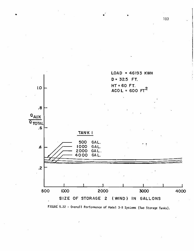
OAUX

TOTAL

*6 t TANK I

LOAD = 46193 KWH

D = 32.5 FT.

HT = 6 0 FT. ACO L = 6 0 0 F T ~

4 0 0 0 GAL.

500 1000 2000 3000

S I Z E OF STORAGE 2 (WIND) IN GALLONS

FIGURE 5.22 - Overall Performance of lilodel 3-8 Systems (TWO Storage Tanks).

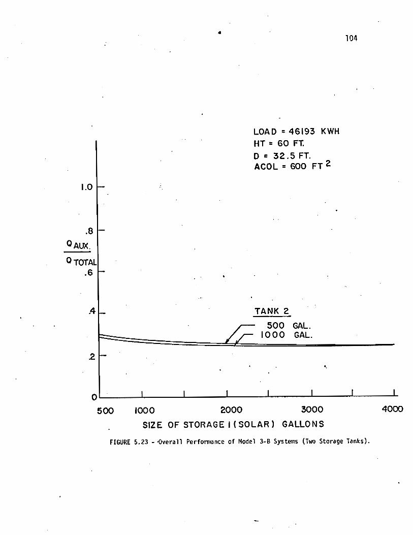
LOAD = 46193 K W H HT = 6 0 FT. D = 32.5 FT. ACOL = 600 FT

SIZE OF STORAGE I (SOLAR) GALLONS

1.0

.8

Q AM.

Q TOTAL .6

.4

FIGURE 5.23 - .Overall Performance of Model 3-8 Systems (Two Storage Tanks).

-

.-

-

- TANK 2

5 0 0 GAL. 1000 GAL.

2

0

,

- 0.

1 I 1 I 1 I I

LOAD = 4 6 1 9 3 KWH/yu

HT = 6 0 FT.

600 FT' (2000 GAL.) . -.- 800 F T ~ (2000 GAL)

200 ( 2000 G A L )

600, (2 12030 GAL)

BLADE DIAMETER , FT

FIGURE 5.24 - Two Storage Tanks Systems' Performance Vs. One Storage Tank Systems.

heat ing requirements, where the e x t r a energy i n p u t cannot be stored.

F igu re 5.24 represents a coinparison between the performance o f the

fo l l ow ing f o u r systems: a v a r i a b l e s i z e c o l l e c t o r s o l a r o n l y system, a

v a r i a b l e b lade diameter wind o n l y system, a combined -so la r and wind system

w i t h v a r i a b l e c o l l e c t o r and blade. s i z e and one storage tank, and a

combined s o l a r and wind system w i t h v a r i a b l e c o l l e c t o r and b lade s i z e

w i t h two storage tanks, ( a l l s torage tanks and baseboard heater s i zes

are kept cons tant a t 2000 ga l l ons and 50 f e e t r e s p e c t i v e l y ) . A t the

lower blade diameters the performance of t he one storage tank system i s

h igher than t h a t o f t he two s torage system. The main reason f o r t h i s

r e s u l t i s t h a t w i t h two tanks the heat losses f rom the tank w a l l s a re

g rea te r than the losses from a s i n g l e tank system. As expected, a t

h igher blade diameters the two tank system has a h igher performance,

however, i t i s a very s l i g h t increase over t he one tank system.

It i s obvious f rom the prev ious d iscuss ion of the performance o f

t he var ious systems t h a t t h e r e are many component s i z e t r a d e o f f s t h a t

can be considered w i t h the combined windpower and s o l a r thermal systems.

Although t h i s chapter has j u s t considered t h e i r e f f e c t s on energy

requirements, a f u t u r e chapter w i l l cons ider t h e i r e f f e c t s on system

economics.

5.3 Domestic Hot Water Heating A n a l y t i c a l Resu l ts

I n t h i s p a r t o f t he s tudy a domestic h o t water heat ing supply i s

in t roduced -as p a r t o f t h e s o l a r and wind r e s i d e n t i a l space heat ing systems.

For t h i s supply, t he thermal s torage o f t he var ious models p rev ious l y '

descr ibed i s used as a pre-heater f o r t h e domestic h o t water sub-system.

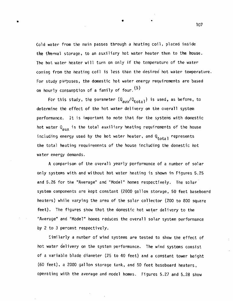
Cold water from the main passes through a heat ing c o i l , placed i n s i d e

the thermal storage, t o an a u x i l i a r y ho t water heater then t o the house.

The ho t water heater w i l l t u r n on o n l y i f the temperature of t he water

coming from the heat ing c o i l i s l ess than t h e des i red hot water temperature.

For study purposes, the domestic ho t water energy requirements are based

on hour l y consumption o f a f a m i l y o f f ou r . (5)

For t h i s study, the parameter (Qaux/Qtotal ) i s used, as before, t o

determine the e f f e c t o f the ho t water d e l i v e r y on t h e o v e r a l l system

performance. It i s important t o note t h a t f o r the systems w i t h domestic

ho t water Qaux i s the t o t a l a u x i l i a r y heat ing requirements o f t h e house

i n c l u d i n g energy used by the h o t water heater, and Qtota, represents

the t o t a l heat ing requirements of the house i n c l u d i n g the domestic ho t

water energy demands.

A comparison o f t he o v e r a l l y e a r l y performance o f a number o f s o l a r

o n l y systems w i t h and w i thou t ho t water heat ing i s shown i n Figures 5.25

and 5.26 f o r the "Average" and "Model" homes respec t i ve l y . The s o l a r

system components are kept constant (2000 g a l l o n storage, 50 f e e t baseboard

heaters) wh i l e vary ing the area o f t he s o l a r c o l l e c t o r (200 t o 800 square

fee t ) . The f i g u r e s show t h a t t h e domestic h o t water d e l i v e r y t o the

"Average" and "Model" homes reduces the o v e r a l l s o l a r system performance

by 2 t o 3 percent respec t i ve l y .

Z i m i l a r l y a number o f wind systems a re tes ted t o show the e f f e c t o f

ho t water d e l i v e r y on t h e system performance. The wind systems cons is t

o f a v a r i a b l e blade diameter (25 t o 40 f e e t ) and a constant tower h e i g h t

(60 f e e t ) , a 2000 g a l l o n storage tank, and 50 f e e t baseboard heaters,

opera t ing w i t h the average and model homes. F igures 5.27 and 5.28 show

"AVERAGE" HOUSE = 32995 k w h / y r

HEAT M C H A N G E R = 50 FT.

T A N K = 2000 GAL. HOT W A T E R = 3565 k w h / y r

~ U E C T O R ' AREA, FT.*

F IGURE 5.25 - E f f e c t o f Ho t Water Del i v e r y on So la r System Performance.

1. 0

-80

.€Q W I T H DOMESTIC HOT WATER SUWLY

-

.40

.20

0 0 200 400 600 800 loo0

-

-

C

I I I

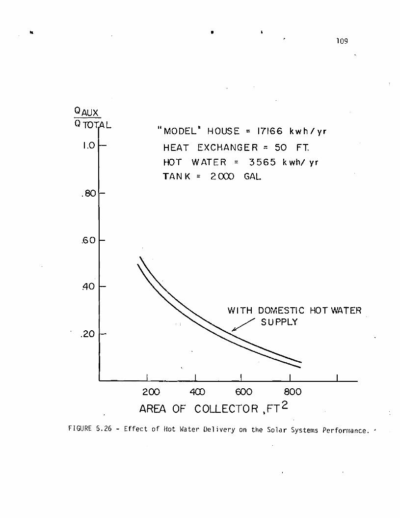
"MODEL" HOUSE = 17166 k w h / y r

H E A T E X C H A N G E R = 50 FT

HOT W A T E R = 3565 k w h / y r

T A N K = 2000 GAL

FIG l lRE 5.26 - E f f e c t o f H o t \ l a t e r D e l i v e r y on t h e S o l a r Systems Per formance. *

Q AUX -- Q TOTAL

1.0

.80

.GO

40

. 20 -

-

-

-

-

W I T H DOMESTIC HOT WATER

I I I I I

200 400 600 800

A R ~ OF COLLECTOR ,FT*

" A V E R A G E I' HOUSE = 32995 k w h / y r

HEAT EXCHANGER = 50 FT

HT = 6 0 FT.

TANK = 2000 GAL

HOT WATER = 3565 k w h / y r

WITH DOMESTIC HOT WATf3 SUPPLY

BLADE DIAMETER, FT.

FIGURE 5.27 - E f f e c t o f Hot Water D e l i v e r y on t h e wind System Perfornmnce.

Q TOTA L

" MODEL " k-IOIJSE

HT = 6 0 FT

HEAT EXCHANGEf;? 50 FT.

TANK = 2030 G A L HOT WATER = 3 5 6 5 k w h / yr

d

-

-

-

WITH DOMESTIC HOT WATER SUPPLY

BLADE DIAMETER, FT.

FIGURE 5.28 - E f f e c t o f Hot Water D e l i v e r y on t h e Wind System Pe r fo r~~ iance .

t h a t hot water del ivery reduces the overall system performance by 4

percent fo r the model house and 3 percent f o r the average house.

The e f f e c t of domestic hot water heating on the combined so l a r and

wind systems (Model 3-A) fo r both the "Average" and "Model " homes i s shown

in Figure 5.29. The combined system cons i s t s of a var iable co l lec to r

2 area ( 0 t o 800 f t ) , a 32.5 foo t blade diameter, a 60 foo t tower, a 2000

gallon s torage, and a 50 foo t baseboard heater . The overall performance

of these systems i s 2 t o 4 percent l e s s than the system performance of

the combined so l a r and wind systems without hot water del ivery.

Since the e f f e c t of domestic hot water heating on the overal l

performance, based on the t o t a l of household and water heating, was

shown t o be small , i t i s important t o determine ' how much of the domestic

hot water energy demand i s delivered by these systems. Thus, in the

fol lowing discussion of r e s u l t s , the auxi 1 i a ry energy used f o r domestic

hot water heating i s presented a s a percent of the t o t a l domestic hot

water energy requirement. For a wind system with a variable blade diameter

(25 t o 40 f e e t ) , 60 foot tower, 2000 gallon storage tank and the "Average"

house heating 1 oad the auxi 1 i a ry hot water energy requirements, Figure 5.30,

range from 40 t o 11 percent respectively. Figure 5.31 ,shows t h a t a so l a r

system operating with the "Average" house load and a var iable co l lec to r

area (200 t o 800 f t 2 ) with 2000 gallon storage tank requires 64 t o 20 per-

cen t , respect ively , of the domestic hot water energy demands t o be

delivered from an aux i l i a ry source. Figures 5.32 and 5.33 represent the

aux i l i a ry domestic hot water energy requirements of wind and so l a r systems

a s a function of blade diameter (60 f o o t tower) and co l l ec to r area

D = 32.5 FT.

HT = 6 0 FT. HEAT EXCI-]ANGER = S O FT. TANK = 2000 G A L .

F I G U R E 5 . 2 9 - E f f e c t o f Ho t Water D e l i v e r y on Combined Wind and S o l a r Systems Performance.

1.0 -

.80 -

.60 -

.40 - WITH DOMESTIC HOT

.20 - 'AVER AGE "

I' MODEL" HOUSE HOUSE

0 I I 1 I

HOT WATER = 3565 k w h / y r

'AVERA-GE " HOUSE H T = 6 0 FT.

BLADE DIAMETER , FT.

FIGURE 5.30 - A u x i l i a r y Energy Needed f o r Doniestic Hot Water Heat ing.

HOT W A T E R = 3565 k w h / y r

"AVERAGE " HOUSE

FIGURE 5.31 - A u x i l i a r y Energy Needed f o r Doniest ic Hot Water Hea t ing .

HOT W A T E R = 3565

" MODEL" HOUSE

BLADE DIAMETER , FT. .,

FIGURE 5.32 - Auxi l ia ry Energy Needed f o r Hot Water Heating.

HOT WATER = 3565 k w h / yr

" MODEL " HO ME

FIGURE 5.33 - A u x i l i a r y Energy Needed f o r Domestic Hot Water Heating.

r e s p e c t i v e l y . Both systems operate w i t h a 2000 g a l l o n s to rage tank and

the "Model" house hea t i ng load. The a u x i l i a r y h o t water energy r e q u i r e -

ment o f t h e wind system, shown i n F igu re 5.32, ranges froni 30 t o 3 percent

f o r 25 t o 40 f o o t b lade d iameter r e s p e c t i v e l y . For t h e s o l a r system,

F igu re 5.33, t h e a u x i l i a r y demands range from 55 t o 11 percent f o r 200

t o 800 square f o o t c o l l e c t o r area r e s p e c t i v e l y . S i m i l a r l y , F i g u r e 5.34

shows t h e a u x i l i a r y domestic h o t water requ i rements of t h e combined s o l a r

2 and wind systems a s a f u n c t i o n o f t h e c o l l e c t o r area ( 0 t o 800 f t ). The

systems operate w i t h t he "Average" house l o a d and use a 32.5 f o o t b lade

d iameter w i n d m i l l , 60 foo t tower, and 2000 g a l l o n s torage tank. The

2 f i g u r e s shows t h a t f o r 800 ft c o l l e c t o r t h e a u x i l i a r y demand i s approx imate ly

2 2 percent w h i l e f o r a 200 f t c o l l e c t o r i t i s 10 percent o f t h e t o t a l

domest ic h o t water energy requirements. For t he "Model1' house t h e

combined s o l a r and wind systems supply a l l t h e h o t water energy demands.

5.4 Systems Performance a t Other S i t e s

S o l a r and wind d a t a have been recorded a t t he U n i v e r s i t y o f Massachu-

s e t t s , Amherst and o t h e r s i t e s i n t h e New England area s ince June 1975.

Therefore, i n t h i s s e c t i o n a sample da ta f rom these s i t e s w i l l be used t o

compare t h e performance o f t h e s o l a r and wind systems a t these s i t e s w i t h

t h e r e s u l t s ob ta ined p r e v i o u s l y f rom t h e B lue H i l l s , Massachusetts and

Har t f o rd , Connect icut s o l a r and wind da ta r e s p e c t i v e l y .

Table 5.7 represents t h e average monthly s o l a r i n s o l a t i o n on a v e r t i c a l

su r face f o r bo th Amherst and B lue H i l l s data. Also, Table 5.8 shows t h e

usefu l s o l a r energy d e l i v e r e d t o t h e "Average" house, a t t h e two s i t e s ,

2 by means of a 200 ft s o l a r c o l l e c t o r v e r t i c a l l y mounted, a 2000 g a l l o n

s to rage tank, and 50 ft. baseboard heaters s o l a r system. The r e s u l t s g iven

HOT WATER = 3565 kvrh / y r

'AVERAGE" HOUSE

0 = 32.5 FT.

HT = 60 FT.

COLLECTOR A R E A , FTZ

FIGURE 5.34 - A u x i l i a r y Energy Mecded f o r Hot Water eating Using a Combined S o l a r and Wind System.

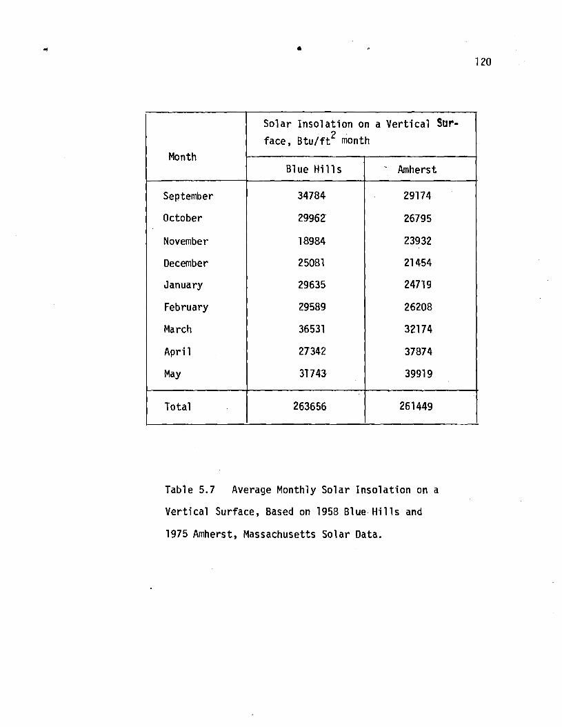
Table 5.7 Average Monthly So lar I n s o l a t i o n on a

V e r t i c a l Surface, Based on 1958 Blue. H i1 1s and

1975 Amherst, Massachusetts So lar Data.

Month

-.

September

October

November

December

January

February

March

Apr i 1

May

To ta l

So la r I n s o l a t i o n on a V e r t i c a l Sur- 2 face, B t u / f t month

- B lue H i l l s

34784

29962

1 8984

25081

29635

29589

36531

27342

3T743

263656

- Amherst

29174

26795

23932

21 454

24719

26208

321 74

37874

3991 9

261 449

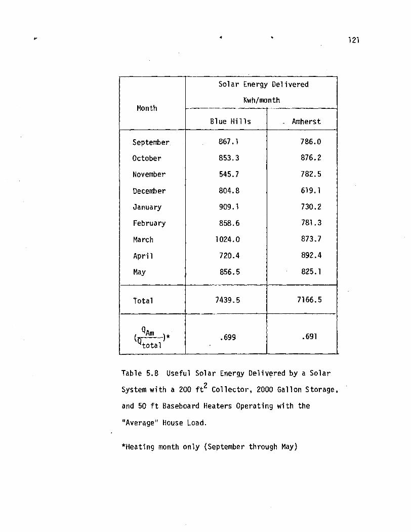
Table 5.8 Useful Solar Energy Delivered by a Solar

2 System w i t h a 200 f t Collector, 2000 Gallon Storage,

and 50 f t Baseboard Heaters Operating w i t h the

-

Month

September

October

November

December

January

February

March

Apri 1

May

Total

Q ~ m (o-)*

to ta l -

"Average" House Load.

*Heating month only (September through May)

- Sol a r Energy Del i vered

Kwhlmonth ----- Blue Hi l l s

867.1

853.3

545.7

804.8

909.1

858.6

1024.0

720.4

856.5

7439.5

.699

- Amherst

786.0

876.2

782.5

619.1

730.2

781.3

873.7

892.4

825.1

7166.5

.691

i n t he tab les show t h a t the t o t a l s o l a r i n s o l a t i o n s and the use fu l s o l a r

energy d e l i v e r e d over the heat ing months a t bo th s i t e s a re approximately

t h e same. As would be expected, t h i s i s due t o t h e f a c t t h a t bo th Amherst

and Blue H i l l s have the same l a t i t u d e and s i m i l a r c l imates .

F igure 5.35 represents a comparison o f t h e wind o n l y system performance

a t th ree d i f f e r e n t s i t e s : 1) Mount Tom, Massachusetts, 2) N o r t h f i e l d ,

Massachusetts, and 3) Har t fo rd , Connecticut. Resul ts a re g iven as a

f u n c t i o n o f t h e b lade diameter and f o r 60 ft. tower, 2000 g a l l o n storage

tank, 50 ft. baseboard heaters and t h e "Average" house load f o r t e n months

o n l y (September through June).

One can see from the f i g u r e t h a t a 32.5 ft. b lade diameter wind system

loca ted a t Mount Tom, Har t fo rd , o r N o r t h f i e l d w i l l supply 100, 70, o r 38

percent o f t h e "Average" house hea t ing requirements r e s p e c t i v e l y . There-

f o r e t h e choice o f s i t e l o c a t i o n f o r wind systems i s very impor tant i n

determi n i ng t h e system o v e r a l l performance.

Q AUX I * "AVERAGE" HOME

HT = 6 0 FT. STORAGE = 2000 GALUINS H.T. = 50 FT.

BLADE DIAMETER , FT

FIGI1P.E 5.35 ldind Svstems Performance a s a Funct ion o f S i t e and Blade Diameter.

* Based on ten months (September through June).

C H A P T E R 6

THE SYSTEM ECONOMIC MODEL

6.1 Background - The economical f e a s i b i l i t y o f s o l a r home heat ing and c o o l i n g has

been the sub jec t of many recent s tud ies . I n a l l o f these system s tud ies ,

d i f f e r e n t economic methods and cond i t i ons were employed. A summary o f

t he most important o f these s tud ies and t h e i r conclusions fo l lows.

(1 ) General E l e c t r i c Corr~pany: ) Th is study was performed by

G. E. f o r t h e Nat ional Science Foundation t o determine the techn ica l ,

economical, s o c i a l , and environmental problems t h a t might r e s u l t f rom

using the s o l a r based heat ing and coo l i ng systems. Cap i ta l cos ts o f

t he s o l a r and conventional systems were determined us ing r e a l p r i c e s

(non- in f l a t i ona ry ) and inc luded t h e c o s t o f t h e conventional system based

on the type o f f u e l used, t h e c o s t of s o l a r panels, storage tank, the

d e l i v e r y system, and mod i f i ca t i ons t o the b u i l d i n g s t ruc tu re . The opera t ing

c o s t o f t he system inc luded maintenance and repa i r s , a u x i l i a r y f u e l cos t ,

i n t e r e s t r a t e , c a p i t a l i z a t i o n c o s t and associated tax savings, and system

usefu l l i f e . Also, t h e l i f e cyc le cos ts were developed f o r compet i t i ve

conventional, and sol a r systems, t o determine t h e * most cos t e f f e c t i ve

over the system's useful l i f e . Fuel p r i ces were based on ac tua l basel ine

r e t a i l f u e l cos ts and upper l i m i t r e t a i l fuel costs.

The f o l l ow i ng a r e t h e i r r e s u l t s obtained from comparing approximately

2500 i n d i v i d u a l l i f e cyc le costs f o r base l ine fuel cos ts and upper l i m i t

fue l costs:

1. Heat ing o n l y systems a re cos t -e f fec t ive when compared t o e l e c t r i c

res is tance heat ing systems i n approximately 85% o f the cases us ing base-

l i n e fuel costs, and i n 94% o f the cases using upper l i m i t f u e l costs.

2. Cool ing on ly systems a re n o t c o s t - e f f e c t i v e f o r e i t h e r basel ine

o r upper l i m i t f u e l costs.

3. Heating and cool i n g systems a re c o s t - e f f e c t i v e when compared

w i t h e l e c t r i c res is tance heat ing systems i n 65% o f the cases us ing base-

l i n e f u e l and 76% i n the cases using upper l i m i t f u e l costs.

( 2 ) Westinghouse E l e c t r i c corpora t i o n : (38'39y40) Thi s study inc luded

a cos t ana lys is o f th ree s o l a r systems: heat ing only, so lar -ass is ted heat

pump, and heat ing and cool ing. To compare these systems w i t h conventional

heat ing and c o o l i r g systems Westinghouse used the l i f e - c y c l e costs approach.

Costs inc luded the s o l a r c o l l e c t o r , storage subsystem, heat exchanger,

c o o l i n g subsystem, supplemental conventional heat ing equipment, and

operat ion and maintenance costs. An annual i n t e r e s t r a t e o f 8 percent

was charged on the c a p i t a l and 7% and 5% i n f l a t i o n ra tes were charged f o r

the fue l and equipment respect ive ly . Based on these ra tes the present

value o f both s o l a r and conventional systems were determined w i t h the

assumption t h a t a l l supplemental energy f o r the s o l a r systems was na tu ra l

gas. The s o l a r systems were evaluated f o r cos t a t performance l e v e l s o f

50 and 80 percent s o l a r dependency. The systems costs were studied f o r

a number o f representa t ive geographic regions and d i f f e r e n t types o f

bu i ld ings.

The W'estinghouse conclusions and recomnendations were:

1. It i s economical ly imprac t i ca l t o design a 100 percent heat ing

and coo l ing s o l a r system.

2. A t present p r i c e s very few s o l a r systems compared favorably

w t t h conventional systems. But t h e 1985 p r i c e s suggest t h a t s o l a r heat ing

and cool i ng systems w i 11 be compet i t i ve w i t h conventional systems.

(3 ) TRW Systems Study: (8'41'42) The TRW study-was performed f o r

d i f f e r e n t c l ima te cond i t i ons and var ious b u i l d i n g types i n four teen

selected c i t i e s . A c o s t ana lys i s program was developed which inc luded

the cos t o f t he equipment, i n s t a l l a t i o n , a p r o f i t f a c t o r and a u x i l i a r y

f u e l and furnace. A c a p i t a l c o s t approach was chosen fo r i t s independence

o f i n t e r e s t r a t e , fue l r a t e and amor t i za t i on period. Based on the c o s t

of fue l saved per year a payback pe r iod was ca lcu la ted by d i v i d i n g the

c a p i t a l c o s t by the fuel cost . Annual costs and present values were a l s o

ca l cu la ted f o r compari son w i t h conventional systems' costs.

The r e s u l t s of TRW economical ana lys i s are:

1. So lar energy shows a c o s t advantage f o r h o t water heat ing systems.

2. Present c o s t o f s o l a r systems should be reduced s u b s t a n t i a l l y i n

order f o r t he s o l a r system t o be compet i t ive.

3 . The market f o r s o l a r systems w i l l increase r a p i d l y i f the system's

s t r u c t u r e i s i n teg ra ted i n the design o f the b u i l d i n g , which w i l l reduce

t h e c a p i t a l cos t .

(4) Lo f and Tybout: (12913'15) The i r e a r l y economical s tud ies were

based on cos ts est imated from experimental s o l a r space heat ing and coo l i ng

systems, commercial s o l a r water heaters and o t h e r commercial conventional

heat ing syitems. Cap i ta l c o s t of a1 1 system components were expressed as

func t i ons o f s o l a r c o l l e c t o r area. Two p r i c e s were adopted i n the ana lys is :

a h igh p r i c e f o r present system costs, and a lower p r i c e f o r fu ture costs.

Also, c a p i t a l cos ts were reduced t o annual cos ts us ing s i n k i n g fund

d e p r e c i a t i o n methods. When compared t o convent iona l systems, t he annual

c o s t o f t h e s o l a r systems i nc luded a u x i l i a r y f u e l and o p e r a t i o n a l cos t s .

I n o rde r t o min imize t he c o s t o f t h e s o l a r systems L o f and Tybout considered

d i f f e r e n t combinat ions o f t he system components. They se lec ted the b e s t

combinat ions between t h e s o l a r systems and t h e complementary convent iona l

systems w i t h t h e f o l 1 owing r e s u l t s :

1. The optimum combinat ion f o r home h e a t i n g i s a combined s o l a r

and e l e c t r i c system.

2. S o l a r systems a r e c o s t c o m p e t i t i v e w i t h convent iona l e l e c t r i c

sys tems.

3 . S o l a r hea t i ng c o u l d compete w i t h gas and o i l hea t i n west and

southwest reg ions o f t h e U.S.

4. Hot water hea t i ng systems' cos t s a r e w i t h i n t h e range o f conven-

t i o n a l f u e l cos ts .

5. The c o s t o f s o l a r energy f o r h e a t i n g and c o o l i n g i n areas w i t h

h i g h c o o l i n g loads i s l e s s expensive than f o r e i t h e r hea t i ng o r c o o l i n g

alone. Whi le i n c o l d areas t h e c o s t o f s o l a r energy f o r hea t i ng a lone i s

l e s s than t h e combined h e a t i n g and c o o l i n g cos t .

I n t h e pas t a few economic s t u d i e s of windpower systems have been

c a r r i e d o u t t o determine t h e f e a s i b i l i t y o f us ing wind systems t o generate

e l e c t r i c i t y . Go ld ing ' s s tudy (26) suggested t h a t t h e c o s t per r a t e d kwh

o f e l e c t r i c i t y . produced decreases w i t h inc rease i n s i z e and o u t p u t o f t h e

wind system. A NASA s tudy (45) showed t h a t t h e c a p i t a l c o s t o f l a r g e u n i t s

100 kW wind systems w i l l u l t i m a t e l y reach 1500 do1 l a r s p e r k i l o w a t t i n s t a l l e d .

These economical s tud ies i n genera l showed, by u s i n g t h e break-even method,

tha t for a combined conventional wind system, the break-even costs will

occur, fo r medium to large scale machines, when the price of 011 r i ses

to (10-1 5) do1 1 ars per barrel.

6.2 System's Individual Components Cost Analysj s

This econonlical study determines the cost of the solar and wind

systems fo r two different representative cases: 1 ) present cost which i s

based on limited production rates; 2) future cost based on mass-production

rates. A1 so, the analytical model takes into consideration the ef fec t

of inflation on present prices. The cost of each component i s developed

from a variety of sources such as: analysis of materials costs, prices

obtained from manufacturers, previous economical studies, the University

of Massachusetts' actual system cost , and other standard cost estimation

methods. All costs used in the following analysis a re based on 1975

prices unless otherwise mentioned.

6.2.1 Storage Cost. CST

The cost of the storage subsystem depends mainly on the type of

storage used. For th i s study, only water thermal storage i s discussed in

de ta i l , since i t i s one of the most economical types of storage for home

heating and i t i s readily available. Storage size, material and insulation

are the basic factors tha t control the cost of the water storage subsystem.

Table 6.1 sumnarizes a l i s t of storage tank prices normalized to dollars per

gallon of storage. The l i s t includes the cost of the UMass storage tank

which was fabricated while this study was in progress.

From the Table one can notice two ranges of prices, 0.73 to 1 .OO and

0.40 to 0.54 dollars per gallon of water, which are assumed t o represent

the present and the future cost of the storage subsystem respectively. Based

Company Source

Wes t inghouse (38) I

Westi nghouse (40 )

Westinghouse (40)

Est imated Westinghouse

Bateman C o n s t r u c t i o n company (40)

Univ . o f Mass. (Presen t c o s t )

Univ . o f Mass. (Fu tu re c o s t )

D u f f i e , e t a1 (44)

N a t i o n a l u r au o f Standards 8457

General E e c t r i c company (1 1

11

I 1

L o f & Tybout (13)

Type (Ma t e r i a 1 ) S i ze I 1 Ga l l ons ) I

Re in fo r ced 1000 Concrete

S tee l ( I n s u l a t e d ) 2000 .

F i berg1 ass

Q u a n t i t y P roduc t i on

I n s u l a t e d ( I n s t a l l e d )

Concrete ( I n s u l a t e d )

I 1

Concrete

S tee l , I n s t a l l ed , I n s u l a t e d I loo0 I

Cost $

I Cost

TABLE 6.1 - Storage Cost (Water)

on these values, for th i s study $0.50/gallon was used as the base cost for

future storage systen~s and $0.80/gal. was used as the base cost for present

systems. Figure 6.1 shows average present and future cost as a function

of the storage size. Then average costs are in the analytical program

as the basic price for present a n d future storage subsystems. The storage

total cost, C S T , i s given by

'ST = 'st 'st (6.1)

where Cst i s storage cost per gallon, and V s t i s the volume of storage in

gallons.

6.2.2 Solar Collector Cost, CC

In th i s study the cost of the collector i s based on the use of f l a t -

plate solar collectors using water as the heat removal f luid. This cost

i s derived from several cost analyses and current r e ta i l prices. A number

of factors are taken into consideration in determining the collector cost

such a s : s ize, materials, manufacturing, shipping, and instal lat ion. In

many cases the cost of the collector ref lects the cost of the total solar

system as a function of the collector area a n d i t includes the cost of

pipes, pumps, controls, heat exchangersand instal lat ion. Table 6.2

represents a sumnary of various researcher's present and future costs

for the f la t -p la te solar collector. Also, for future cost purposes,

Table 6.3 gives a detailed breakdown of the cost per unit area of the

collector and i t i s given for one and two glass covers.

~ a s i n g the collector costs on a per area basis, the total cost of the

collector CC i s given by

C~ = CclAc

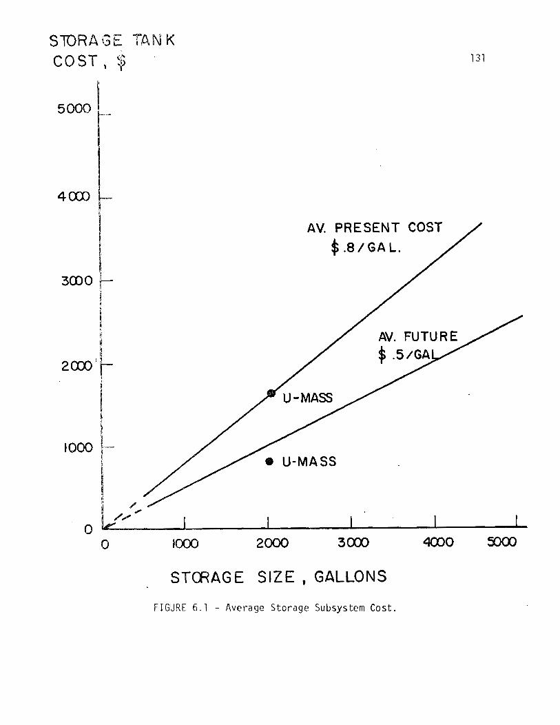
loo0 2000 3000 4000

STCRAGE SIZE , GALLONS

FIGURE 6 . 1 - Average S t o r a g e Subsystem Cost.

Present Cost Future Cost Comnen t s -- M i t r e (46)

G.E. (11 1

UMass (Dixon)

Tybout & Lo f

P r i ce i n c l udes ( c o n t r o l s , pipes, pumps, H . X . ) i n s t a l l e d .

S ing le Glass, i n s t a l l e d

I Double Glass, i n s t a l l e d

Inc ludes (pipes, pumps - - e t c . )

4.0-2.0 Plus ($375 f o r pumps & pipes

Nat iona l u r au 1457 1 - - I n c l udes (pumps, pipes,

o f Stand. con t ro l s , -- e tc . )

Steadman ( 7 ) 1 8.0 I 4.0 1 I n s t a l l e d

Wes tinghouse (38) Plus ($2.32/ f t . f o r p l umbi ng & c o n t r o l s )

Aluminum, double g laze (p lus i n s t a l l a t i o n )

Aluminum, no glaze, p l u s i n s t a l l a t i o n

TABLE 6.2 - So lar C o l l e c t o r Cost

11 - - 2.86 Galvanized i r o n , no glaze, (p lus i n s t a l l a t i o n )

I tern Single Cover* Double-Cover*

Labor & Materials (Mfg. ) 1.69 2.09

Prof i t 35%

Dis t r ibut ion 25%, ( f i r s t l e v e l ) .57 .71

Dis t r ibut ion 40% (second level ) Ins ta l le r /sub-contrac tor 1.15

General Cost 10% .40 .50

Adjustment f o r Shaded Port ion .30 .35

Total Cost 4.70 5.80

* Based on a production r a t e of one mil l ion panels per year .

TABLE 6.3 - Solar Col lec tor Cost (11)

where Ccl cos t o f t he c o l l e c t o r / u n i t area, and A, i s t h e c o l l e c t o r area.

Based on the previous data, two values of Ccl a re assumed f o r present

and f u t u r e cos ts (10 & 5 $lsq ft r e s p e c t i v e l y ) . Thus, the t o t a l c o l l e c t o r

c o s t f o r a g iven area i s shown i n F igure 6.2.

6.2.3 Windmill Cost, CM

Even though the p r i n c i p l e s o f wind systems have been known f o r a long

time, the ana lys i s o f wind systems' cos ts i s a very d i f f i c u l t task and

more o f economical and techn ica l s tud ies a r e needed before an. accurate

and d i v e r s i f i e d model could be developed t o determine t h e system's cos t

as a f u n c t i o n o f t h e number o f blades, blade s ize, e l e c t r i c generator,

tower he ight , t ransmission and c o n t r o l mechanism and o t h e r f a c t o r s .

I n most cases the r o t o r d r i v e s an e l e c t r i c generator and i t .has

been a common p r a c t i c e t o present the cos t o f t he wind system as a f u n c t i o n

o f t he generator r a t e d power output . Table 6.4 represents t h e t o t a l . c o s t s

o f some wind systems as a . funct ion of t he generator r a t e d power output .

The systems could be c l a s s i f i e d by output as: l a r g e (100 kW and up),

medium (10 kW - 100 kW), and small (1-10 kW). From the Table, one n o t i c e s

t h a t small wind systems are the most expensive s ince a l a r g e sum o f the

cos t i s charged towards the tower and i n s t a l l a t i o n and o the r f i x e d costs.

Thus, i n general medium and l a r g e wind systems would produce more energy

and they a r e more economical t o cons t ruc t on a u n i t power basis.

Tables 6.5 and 6.6 represent the c o s t of each system component o f t h e

NASA 100 ku and UMass 25.0 kW wind systems respec t i ve l y . However, i n

comparing the cos ts o f bo th systems i t i s no t i ced t h a t us ing the parameter,

cost/kW, emphasizes the importance of t he generator r a t e d power output only.

COLLECTOR COST, $

COLLECTOR A R E A - f t 2

FIGURE 6.2 - Average Collector Cost.

- -- - -- -

TABLE 6.4 - Wind System To ta l Cost (No Storage)

Source ( r e f . )

Putnam (43)

N A S A ( ~ ~ )

NASA

UMass (47)

llllla s s

Brace I n s t . (43)

Dun1 i t e ( A u s t r a l i a )

I1

E l e k t r o (Swiss)

I1

I1

Jacob (U.S. )

I1

I 1

Cap i ta l c s t 3 x 10- do1 1 a r s

1051

500

150

12.6

6.2

13

2.07

3.11

2.51

3.24

4.89

3.75

4.0

4.0

?ated power 3utput, kW

1000

1 00

100

25.0

25.0

10

1

3

1.2

2.2

6.0

1.8

2.5

3.0

Cost /output $/ kW

1051

5000

1500

500

250

1 300

2070

1040

2090

1470

81 5

2080

1600

1 300

Cormlien t s

Projected t o ' 71

Present Cost

Future Cost

Present Cost

Future Cost

Present Cost

R e t a i l p r i c e s

11

11

11

11

I#

11

11

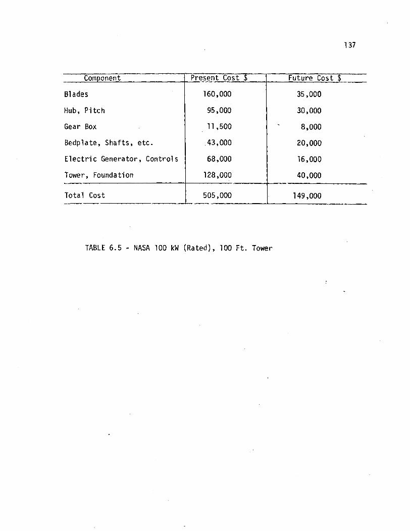
- Component

Blades

Hub, P i t c h

Gear Box

Bedplate, Shafts, e tc .

E l e c t r i c Generator, Contro ls

Tower, Foundation

Tota l Cost

TABLE 6.5 - NASA 100 kW (Rated), 100 F t . Tower

Present Cost $

160,000

Future Cost $

35,000

- - -

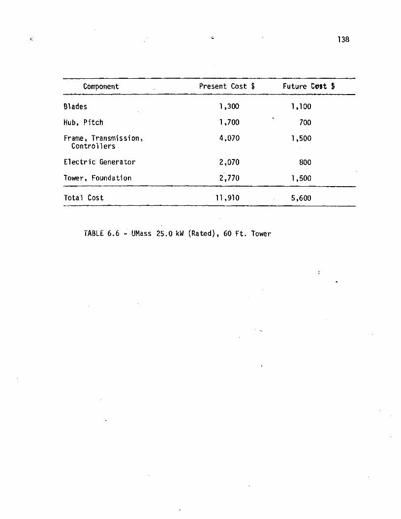
Component Present Cost $ Future Cost $

Blades 1,300 1,100 -

Hub, P i tch 1,700 700

Frame, Transmission, Contro l lers

E l e c t r i c Generator 2,070 800

Tower, Foundation 2,770 1 ,500

Total Cost 11,910 5,600

TABLE 6 .6 - UMass 25.0 kW (Rated), 60 F t . Tower

I n f a c t , (especi a1 l y f o r home heat ing systems) the system o v e r a l l performance

depends on o ther parameters such as: tower height , blades diameter, number

o f blades and o ther system components such as the s i z e o f storage and the

heat d e l i v e r y subsystem. I n t h i s economical ana lys is the t o t a l cos t o f

the system i s based on the f o l l o w i n g cost ana lys is o f each o f the system's

components. Th is d e t a i l e d components' cos t ana lys is w i l l be used t o

determine the cost o f medium s i z e wind systems.

6.2.3a Tower Cost, CT

Since the tower he ight i s an important f a c t o r i n determining the

performance o f the windmil 1 i t i s des i rab le t o express the cost o f the

tower as a f u n c t i o n o f i t s height . Table 6.7 summarizes a number o f

a v a i l a b l e tower costs from var ious sources fo r d i f f e r e n t he ights and

s t ruc tures . Also, Table 6.8 g ives a d e t a i l e d cost ana lys is o f the UMass

tower (47) which cons is ts o f a Stayed Pole Mast, 60 f e e t t a l l , w i t h fou r

dead weight concrete anchors. Pr ices shown i n Table 6.8 are those o f p a r t s

t h a t were purchased from r e t a i l d i s t r i b u t o r s . F igure 6.3 summarizes a1 1

o f t h i s data and gives a graph ica l representa t ion o f the tower cost as

a f u n c t i o n o f he igh t and weight per u n i t he ight . From t h i s f i gu re , one

no t i ces t h a t t h e UMass fu ture tower cos t i s i n the same range o f the

r e t a i l p r i ces obtained from tower manufacturers. Also, t h a t NASA's tower

cos t i s very high due t o e i t h e r over design of the tower s t r u c t u r e o r the

system i s too la rge. Tower p r i c e s used i n the computer ana lys i s are 46

d o l l a r f i o o t and 20 d o l l a r s / f o o t f o r present and f u t u r e cos ts respec t i ve l y .

Other costs could be u t i l i z e d by the program i f needed. The tower t o t a l

cost, CT, i s given by

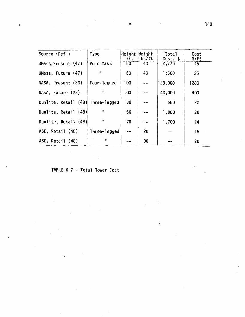
TABLE 6.7 - To ta l Tower Cost

Cost $/Ft 46

25

1280

400

22

20

Dun l i te , Reta i 1 (48)

ASE, R e t a i l (48)

T o t a l Cost, $ 2,770

1 ;500

1 28,000

40,000

660

1,000

Source (Ref. )

UMass, Present (47)

UMass, Future (47)

NASA, Present (23)

NASA, Future (23)

Dun l i t e , R e t a i l (48)

Dun1 i te, Reta i 1 (48)

Height F t . 60

60

100

1 00

30

50

TY pe

Pole Mast

I1

Four- legged

It

Three-legged

11

Weight L b s / f t

40

40

- - - - - - - -

Materials Do1 l a r s

Concrete, including s tee l 800

Four guy wire ropes and f i t t i n g s 700

Sixty f e e t of 10" standard pipe, 40 1 bs / f t j 2 0

Steel footing bal l and socket 200

Upper pole matcher p la te 150

Erection of pole mast 200

Total Cost 2,770

TABLE 6.8 - UMass 60' Tower Cost

TOWER HE1 GHT - f t

F I G U R E 6.3 - Total Cost of Tower.

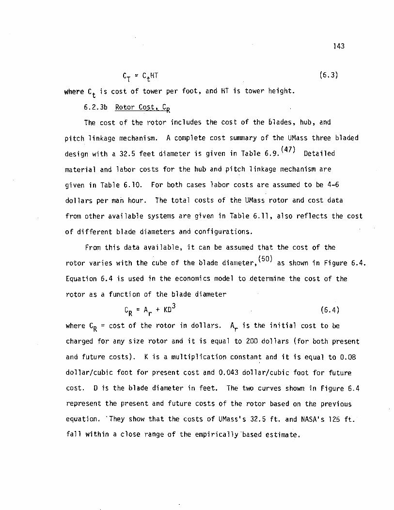
CT = CtHT

where C t i s cost of tower per foo t , and HT i s tower height.

6.2.3b Rotor Cost, CR

The cost of the rotor includes the cost of the blades, hub, and

pitch linkage mechanism. A complete cost summary of the UMass three bladed

design with a 32.5 f e e t diameter i s given in Table 6.9. (47) Detailed

material and labor costs fo r the hub and pitch linkage mechanism a r e

given i n Table 6.10. For both cases labor costs a r e assumed t o be 4-6

do l la rs per man hour. The to t a l costs of the UMass rotor and cost data

from other available systems a r e given in Table 6.11, a lso r e f l ec t s the cost

of d i f fe ren t blade diameters and configurations.

From this data avai lable , i t can be assumed t h a t the cost of the

rotor varies with the cube of the blade diameter, (50) as shown i n Figure 6.4.

Equation 6 .4 i s used in the economics model t o determine the cost of the

rotor a s a function of the blade diameter

where CR = cost of the rotor in dol lars . A, i s the i n i t i a l cost t o be

charged fo r any s i ze rotor and i t is equal t o 200 dol la rs ( f o r both present

and future cos t s ) . K i s a multiplication constant and i t i s equal t o 0.08

dollar/cubic foot fo r present cos t and 0.043 dollar/cubic foot fo r future

cost. D i s the blade diameter in fee t . The two curves shown i n Figure 6 .4

represent the present and future cos t s of the rotor based on the previous

equation. 'They show t h a t the costs of UMass's 32.5 f t . and NASA's 125 f t .

fa1 1 within a c lose range of the empirically based estimate.

I terns Do1 1 a r s

Consuma b l e c ia te r i a1 s .46

Reenforcement m a t e r i a l s 421

Resin and hardner m a t e r i a l s 206

S t e e l m a t e r i a l s (150 I b s ) 4 5

Labor c o s t (77 hours a t $4 /h r ) 308

M isce l laneous . 274

T o t a l 1 ,300

TABLE 6.9 - Cost Summary of UMass Three GRP Blades (32.5 f e e t d i a . )

Components Do1 1 a r s

Flat s t ee l pla te and sheet and sol id bar- stock (237 lb s ) 84

Tubular s t e e l , h u b sockets and standpipe (189 Ibs) 75

Sprockets ( s ix ) 4 1

Pitching chains ( th ree) 30

Bearings , h u b 40 1

Other bearings and bearing materials 99

Steel for the plunger and the cars 20

Bronze materials 84

Ball and n u t assembly and attachments 170

Other s tee l used 18

Labor cost (134 hours, a t $6/hr) 804

Total Cost 1,826

TABLE 6.10 - Cost Estimate o f the UMass Hub and'Pitch Linkages

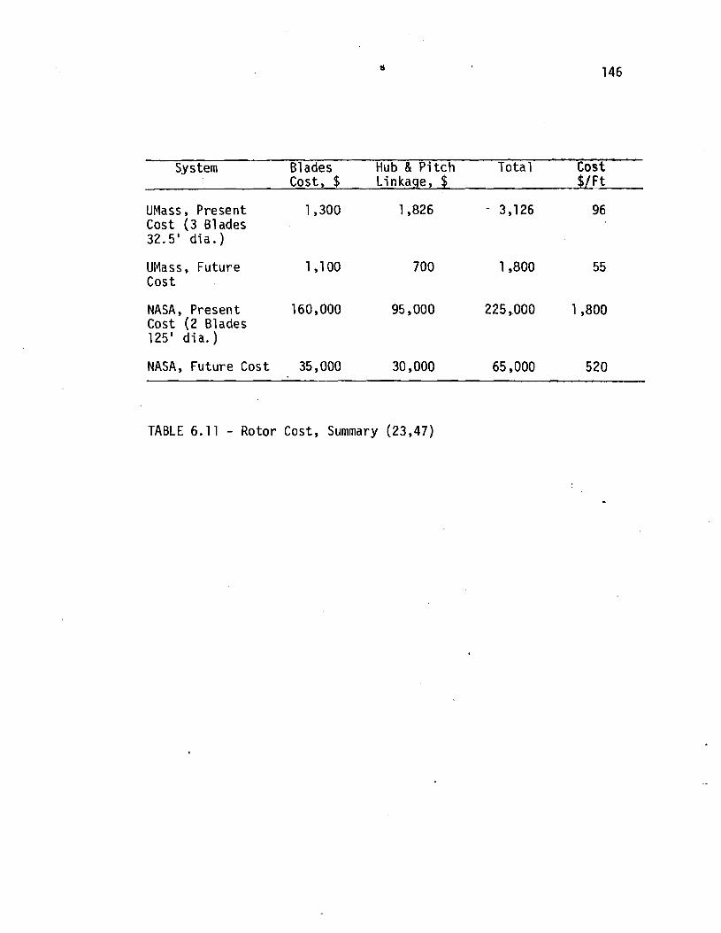
System Blades Hub & P i t c h Total Cost Cost, $ Linkage, $ $/Ft

UMass , Present 1,300 1,826 - 3,126 96 Cost (3 Blades 32.5' d ia.)

UMass, Future 1,100 700 1,800 55 Cost

NASA, Present 160,000 95,000 225 ,.OOO 1,800 Cost (2 Blades 125' d ia . )

NASA, Future Cost 35,000 30,000 65,000 520

TABLE 6.11 - Rotor Cost, Summary (23,47)

6 . 2 . 3 ~ Frame and Transmission Costs, CB

This s e c t i o n covers the c o s t o f s t a t i o n a r y p a r t s o f t h e w+ndmi l l such

as t h e gear box, frame, t ransmiss ion and c o n t r o l s . It i s d i f f i c u l t t o

determine t h e c o s t o f t he s t a t i o n a r y p a r t s o f o t h e r Systems s ince i n most

cases p r i c e s a re quoted f o r t h e e n t i r e w i n d m i l l system. Table 6.12 i s a

c o s t summary o f t h e s t a t i o n a r y p a r t s purchased f o r t h e UMass system.

These cos ts a re used i n t h e present economical model s ince t h e generator

s i z e i s kept t he same throughout t h e a n a l y s i s of t h e system performance.

I n a d d i t i o n , Table 6.13 represents a sample o f t h e present and f u t u r e cos ts

o f the NASA and UMass t ransmiss ion and l i n k a g e mechanisms.

6.2.3.d Generator Cost, C,

The generator cos t i s a f u n c t i o n of i t s r a t e d power ou tpu t and i t i s

determined by choosing a generator s i z e most app rop r ia te f o r a g iven s i t e ,

blade diameter, and tower he igh t . Table 6.14 g ives a summary o f generator

cos ts ob ta ined by t h e UMass and NASA s tud ies . The c o s t o f t h e generator

used i n t h i s economical s tudy i s t h a t o f t he UMass 25.0 kW ( r a t e d ) generator

(s ince i t was used t o determine t h e performance o f the windmil 1 ).

6.2.4 Heat D e l i v e r y System Cost, C,,

The most common types of heat d e l i v e r y systems used i n home heat ing

are: . forced h o t - a i r , ho t water baseboard heaters, o r e l e c t r i c res i s tance

heaters. The c o s t o f t h e d e l i v e r y system depends on the type o f t h e system

and i t s s i ze . Table 6.15 presents a number of h o t water baseboard systems

and t h e i r cos ts p l u s sample a i r and e l e c t r i c system costs. The expanded

use o f any of these systems i n s o l a r and wind hea t i ng i s n o t expected t o

change t h e i r cos t , s i nce heat d e l i v e r y systems have been i n use w i d e l y i n

Speed Up Transmission 1 1,220 I 450

------ 1 tern

p-

blain Frame

Pole Matcher

Switching Logic, F ie ld Cont.

P i t ch Control l e r

Nace l les , Yaw Cont. -------- --

Present Cos t , $

1,075

335

Future Cost , $

400

250

TABLE 6.12 - Cost o f UMass Transmission and Mechanical Cont ro ls ( 4 7 ) .

Total Cost ---

4,145 1,495

Sys tem Transmission Frame and To t a 1 Cost Cost, $ Mech. Cont. $ $ $/ k~

UMass, 26 kW (R), 1,220 2,925 4,145 160 Present

-

UMass, 26 kW (R), 450 1,045 1,495 58 Future

NASA, 100 kW (R), 11,500 43,000 54,500 545 Present

NASA, 100 kW (R), 8,000 20,000 28,000 2 80 Future

TABLE 6.13 - Frame & Transmission Cost (23,47)

UMass , Future 1 25.0 31.1 1 - 8 0 0 1 31

Sys ten1

UMass, Present

NASA, Present 1 100 125 1 68,000 1 680

Rated Power Output k W kVa

25.0 31.1

TABLE 6.14 - Generator Cost, Do l la rs

NASA, Future

Cost $

2,070

100 125 1 16,000 1 160

Cost $/kW __

80

GE ( 1 ) I Water 1 286 1 144 / 6 . 5 $ / f t

M i t r e (46)

L o f & Tybout (12)

N.B.S. (45)

LIMass (47)

Source (Ref. )

Water

TY pe

Water

Water

Water

-- --- P ipes

$ ----

H.X. $

E l e c t r i c

Pumps $

7 $ / f t i n s t a l l e d

Westinghouse (40) 1 A i r I 8 . 4 0 / 1 0 0 f t o f d u c t i n s t a l l e d

TABLE 6.15 - Heat D e l i v e r y System Cost

153

home heating. The on ly increase i n cost w i l l be due t o i n f l a t i o n . I n

t h i s economical study the UMass heat de l i ve r y cost, 465 do l l a r s , was used

since the components were purchased i n New England.

6.3 The Cost o f the A u x i l i a r y Heating System, CAUX

The auxi 1 i a r y system i s needed when the so lar and/or wind system

f a i l s t o supply p a r t o r a l l o f the house heat ing load. Therefore, the

capac i ty o f the a u x i l i a r y heater should be as h igh as the house heating

requirement, even though i n many cases the auxi 1 i a r y heat needed might

be s i g n i f i c a n t l y less . I n t h i s study the a u x i l i a r y system i s assumed

t o be o f the same type (gas, o i l , e l e c t r i c ) as the conventional system

ava i l ab l e t o the buyer. The annual a u x i l i a r y f u e l cost CAUX i s given by:

- C )/EFF 'AUX - (Qaux f (6.5)

where Qaux = the a u x i l i a r y heat requirement i n kWh/yr. and Cf = f ue l

cost per kwh, EFF = e f f i c i e n c y o f the a u x i l i a r y furnace.

The f ue l cost and conventional heat ing system cost a re discussed

i n the next sect ions.

6.4 Fuel and Conventional Heating System Cost, C, and CCoN

The cos t o f heat ing f u e l i s a funct ion of many fac tors w i t h supply

and demand the most important. A l l i nd ica t ions are t h a t supply and demand

a re moving i n the d i r e c t i o n t h a t would increase the cost o f fuel, s ince

demand i s increasing and f ue l sources a re decreasing. The f o l l ow ing

presents a shor t ana lys is o f the 1975 pr ices and the pro jec ted cos t i n

the f u t u r e f o r na tu ra l gas, o i l , and e l e c t r i c i t y . Fuel costs a re normalized

and given sin terms o f cos t per k i l o w a t t o f energy del ivered.

The annual conventional fuel cost, CF, i s g iven by the fo l l ow ing

cF = (Q Cf)/EFF ( 6 . 6 )

where Q i s the t o t a l heat ing load i n kWh/yr and C f i s the f u e l c o s t

per kwh, and EFF = the e f f i c i e n c y o f the furnace.

The c o s t o f conventional system cons is ts o f b a s i c a l l y the same system

components as t h e a u x i l i a r y system the re fo re CCON i s - g i v e n by:

C ~ ~ ~ i = C~~ + C~ +

(6.7)

where CCON i s t h e t o t a l c o s t of conventional system components, CAF

i s the a u x i l i a r y furnace cost, C,, i s d e l i v e r y system cost , and CST i s

the c o s t o f thermal storage.

6.4.1 Natural Gas

Although the use o f na tu ra l gas f o r home heat ing i n the New England

reg ion i s l i m i t e d , i t i s used for heat ing purposes i n o the r p a r t s o f

the country. Therefore, a cos t ana lys is o f na tu ra l gas f u e l and heat ing

system i s conducted i n t h i s study. The heat ing system c o s t inc ludes

furnace cost , duc t ing and i n s t a l l a t i o n charges. Based on var ious sources,

Table 6.16 summarizes 1975 p r i ces of the fuel and t h e system's components

f o r the New England area.

An i n i t i a l average c o s t of .68 cents/kWh was used i n the i n i t i a l

economical model s tud ies w i t h an i n f l a t i o n r a t e o f 7% compounded annual ly .

6.4.2 O i l Cost

I n the recent years o i l p r i c e s have been increas ing r a p i d l y , b a s i c a l l y

dbubl i n g i n t h e l a s t f i v e years. This p r i c e escal l a t i o n i s expected t o

cont inue i n the fu tu re , b u t a t a slower r a t e . Also, i n the New England

region, most o f the o i l consumed i s imported and the Uni ted States govern-

ment has l i t t l e or no c o n t r o l over t h e p r i c e increase.

Table 6.17 g ives a 1975 cos t summary of o i l , o i 1 furnace, pumps, pipes,

TABLE 6.16 - Natura l Gas Cost

4

ffl ffl

Fuel I n f l . Rate, %

Source, Area (Ref. ) Heat Cont n t 3 4 Btu / lO f t

Furnace, Duct I n s t a l l a t i o n , $

M i t re , Boston (46)

Westinghouse, East Coast (40)

General E l e c t r i c , Boston (11)

Massdesign, Cambri dge (49)

E f f i c i e n c y %

1000 1 o3

1051 l o 3

1000 l o 3

1000 l o 3

7 5

65

- -

8 0

Cost $ /cu . f t .

Cost $/kwh

1,700

1,130

- -

2,800

125-250

350 Av.

240

253

- -

7

5.3

- -

.51-.85

1.20

.82

.86

c 0 .r 3' C, a -

- a J ll- C, c a u e

64

cf aJ C, U a J rg r - L V) 3 n " 5 a

W C c n 3 O Y U\

-G

w 7 u l r g O U U\

tr

LL LLS W

C, t aJ s C, 0 t7 0- U r n a

C , a 3 aJC, r m

n

i aJ e , v

aJ U L =3 0 im

e e I M I U J

0 0 0 0

I I I " O n : I

N

CO m CO O L n L D C O

I QI h O O U J M . h 7 7

0 e I 0 e M M M o e w e e N M

m 0 0 0 0 1 UJ a h h h l

0 0 0 0 0 0 0 0 0 3 0 0 0 0 0 a = n a n a

0 e o o o e 7 e e e 7 7 - 7 7

n t 0

e 2 - m Y e U a - a V)

- m a 3 t U J e 0 m - W . 3 C .r 7 w CT) u l -

a n t a J w aJ v, .re .r 0 L . ~ c ~ c , v ) w m + - u l v , w .r- . 3 aJ a E Z n

etc. The table also includes a projected annual inflation ra te on oi l

prices. An average oi l cost of .98 cents/kWh i s used with an inflation

rate of 4% compounded annually.

6.4.3 Electricity Cost

The cost of e lec t r ic heating depends basically on the fuel used to

generate e lec t r ic i ty . Coal, o i l , and nuclear fuels are used to produce

e lec t r ic i ty . All three of these fuels and their basic e lec t r ic power

plants have experienced rapidly rising costs in the past few years. Other

factors also contribute to the high cost of e lec t r i c i ty and make i t the

most expensive of the three heating sources ( o i l , natural gas, and

e lec t r i c i ty ) . However, in spi te of the high cost of e lec t r i c i ty there

i s a significant increase in the proportion of new homes using e lec t r i c i ty

for heating, 33 percent in Mew England. (39)

Table 6.18 represents a range of e lec t r ic i ty and heating system cost

in the New England region. The cost includes base1 ine cost and a fuel

adjustment note charged by the u t i l i t y companies. The table also includes

estimates on annual inflation rates. An e l ec t r i c i ty cost of 4.2 cents/kWh

was used in the analytical program with a 3% inflation rate compounded

annual ly.

6.5 Total and Annual System Cost

The total cost of the solar and/or wind systems include the cost of

acquisition of a l l the systems components described ea r l i e r in th i s Chapter.

the cost of maintenance and operation, and the cost of the auxiliary system.

Total cost i s then reduced into annual cost to be compared with the yearly

cost of the conventional heating system. Annuities are calculated using

- -- -----.-up.- -- Source (Ref. I Heat Content EFF Cost H.X. & Cont ro ls IHFL - ~ . ~~

BtuIkWh % t / kklh----- $ Rate --- "/J

Du f f i e & 341 3 9 5 Beckman (44) 2-4 - 3.5

M i t r e (46) 11 9 5 3- 4 1,500 - Westinghouse (40) " 100 4.0 - 2

Massdesign (49) I I 100 3.4 1,100 3

G.E.. (11) 11 95 2-4 - - West. Mass

Elec. b i l l s I I

TABLE 6.18 - E l e c t r i c i t y Cost

twenty years ' amor t iza t ion per iod and a 6 t o 8 percent i n t e r e s t r a t e

compounded annual ly. As w i l l be discussed, a computer program has been

designed t o ca l cu l a te the costs o f three d i f f e r e n t systems:

A. So lar on ly : which cons is ts of a so l a r co l l ec to r , heat de l i ve r y

subsystem, storage and a u x i l i a r y furnace. The t o t a l cost o f t h i s system

i s given by the fo l lowing equation:

CS1 = Cc + CD + CsT + CAF (6.8)

where CS1 = system t o t a l cos t i n do l l a r s , CAF = cost of a u x i l i a r y furnace

i n do l la rs .

B. Wind only: This system includes the windmi l l , the heat de l i ve r y

subsystem, storage, and an a u x i l i a r y furnace. The t o t a l cost, CS2, o f

t h i s system i s :

CS2 = Cw + CD + CsT + CAF (6.9)

where C,,, = CR + CB + CT + CG.

C. So lar and wind: This system i s a combination o f the previous

two systems w i t h one storage, one heat del i v e r y subsystem, and one a u x i l i a r y

furnace. The t o t a l cost, CS3, i s equal t o the fo l lowing:

CS3 = C w + Cc + CD + CsT + CAF (6.10)

The annual cost of any o f these systems, ACS, i s given by equation 6.10.

ACS = CS.R + CAUX (6.11)

where CS i s the t o t a l cos t of the system and R i s a f i x e d amor t iza t ion

r a t e given by

where ir = percent i n t e r e s t r a t e , and n = amor t iza t ion per iod i n years.

The annual c o s t o f t h e conven t i ona l system i s t h e sum o f t h e annual

con~ponents c o s t and t h e annual conven t iona l f u e l c o s t and i t i s g i ven by:

ACON = CCON R + C F (6.12)

where ACON i s t h e annual conven t i ona l system c o s t .

C H A P T E R 7

ECONOMIC STUDY RESULTS

7.1 I n t r o d u c t i o n -

This chapter combines the r e s u l t s obta ined from the energy model

w i t h those from the cos t ana lys i s model o f t h e previous chapter. System

cos ts a r e thus a f u n c t i o n o f t h e i r performance as we l l as t h e i r o v e r a l l

con f igu ra t i on .

I n order t o compare the cos t o f t he s o l a r and wind systems w i t h the

conventional heat ing systems, the fo l l .owing th ree basic costs were ca lcu la ted:

1) The t o t a l cos t o f the conventional heat ing system which inc ludes the cos t

o f a1 1 the system components, operat ion, and maintenance, 2) The t o t a l cos t

o f t he s o l a r and/or wind system which cons is t s o f the c a p i t a l cos t o f the

system components, ope ra t i on, maintenance, and aux i 1 i a r y system, and 3) The

annual cos ts of the so la r , wind, s o l a r and wind, and the conventional

systems. The annual cos ts i nc lude the average y e a r l y f u e l c o s t f o r t h e

conventional and a u x i l i a r y heat. It i s impor tant t o note t h a t the f u e l

p r i c e s inc luded i n t h e annual cos ts o f t he systems a r e the average p r i c e s

over 20 years (1975 t o 1995). Annual costs were obtained by amor t i z ing

the t o t a l system c o s t over 20 years a t an 8 percent i n t e r e s t r a t e .

7.2 Economics Computer Ana lys is

The cos t of the wind and s o l a r system described i n the previous chapters

was determined by means o f an a n a l y t i c a l computer program t h a t used the

c o s t ana lys i s r e s u l t s o f t he system components g iven i n Chapter 6. Costs

were ca l cu la ted as a func t ion o f the s i z e of t h e system components such as:

b lade diameter, tower height , c o l l e c t o r area, storage s ize , house heat ing

load, and the a u x i l i a r y heat ing requirements o f the system.

F igure 7.1 represents the b lock diagrarii o f the coniputer program. The

program ca lcu la tes the present and f u t u r e c o s t o f the f o l l o w i n g : 1) The

s o l a r system components, 2) The wind system components, 3 ) The storage

and the heat d e l i v e r y system, 4) Cap i ta l cos t o f t he reniaining system

components (no t i n c l u d i n g auxi 1 i a r y heat) , 5) Annual c o s t o f the system

based on 20 years ' amor t i za t i on and 8 percent i n t e r e s t r a t e (annual cos t

inc ludes annual a u x i l i a r y system cost , and the a u x i l i a r y f u e l c o s t averaged

over the amor t i za t i on per iod) , and 6) The c a p i t a l and annual cos t of the

conventional heat ing systems ( fo r na tu ra l gas, o i 1 , and e l e c t r i c systems).

The program a l s o ca l cu la tes the present and fu tu re cost , w i t h 5 year

increments, o f o i 1, na tu ra l gas, and e l e c t r i c i t y . A more d e t a i l e d

descr , ip t ion o f t h i s computer program w i l l be g iven i n Appendix B .

7.3 The UMass Model 3-A System Cost

A sample o f the output from t h i s phase o f work i s g iven i n Table 7.1.

Based on the work o f t h e previous chapter, i t presents t h e present and

f u t u r e cos t o f t h e Uillass Model 3-A system ( t h i s system features a 32.5

f e e t w indmi l l mounted on a 60 foo t tower, a 200 square fee t , v e r t i c a l

mounted, f l a t - p l a t e c o l l e c t o r , a 2000 g a l l o n water thermal storage tank,

and a 50 foo t baseboard h o t water heat de l i v e r y system). A1 so, i n order

t o determine the system's annual costs, t y p i c a l data and assumptions are

shown i n Table 7.2. The t a b l e shows present f u e l cos ts i n dol lars/kWh

and t h e i r corresponding i n f l a t i o n ra tes .

7.4 Other Systems Costs

It i s des i red t o compare s o l a r and wind w i t h conventional systems on

FIGURE 7.1 - B l o c k D i a g r a m o f E c o n o m i c s C o m p u t e r P r o g r a m .

LOAD, SYSTEM REQUIREMENTS

V - CONVENTIONAL SYSTEM COST N. GAS, O I L , ELEC.

AVERAGE AND FUTURE FLlEL COSTS.

-

<

?

TOTAL COST OF SOLAR AND/OR WIND SYSTEMS. (PRESENT & FUTURE)

ECONOMICS MAIN

PROGRAM

-- Y ANNUAL CONVENTIONAL SYSTEM COST. -

v ANNUAL CONVENTICINAL & AUX. FUEL COST.

\Y

ANNUAL SOLAR/WI ND SYSTEM COST. (PRESENT & FLITURE)

v -

4 > ANNUAL COST SOLAR/WIND SYSTEM & AUXIL IARY FUEL & CONVEHTIONAL SYSTEM.

load, and t h e aux- i l i a r y h e a t i n g requi ren ients o f t h e system.

F i g u r e 7 .1 r ep resen t s t h e b l o c k diagrani o f t h e computer program. The

program c a l c u l a t e s t h e p resen t and f u t u r e c o s t o f t h e f o l l o w i n g : 1 ) The

s o l a r system co1.l-~ponents, 2 ) The wind system components, 3 ) The s to rage

and t h e hea t d e l i v e r y system, 4 ) C a p i t a l c o s t o f t h e rema in ing system

components ( n o t i n c l u d i n g a u x i l i a r y h e a t ) , 5 ) Annual c o s t o f t h e system

based on 20 y e a r s ' a m o r t i z a t i o n and 8 pe rcen t i n t e r e s t r a t e (annual c o s t

i n c l u d e s annual a u x i l i a r y system cos t , and t h e a u x i l i a r y f u e l c o s t averaged

ove r t h e a m o r t i z a t i o n p e r i o d ) , and 6 ) The c a p i t a l and annual c o s t o f t h e

conven t iona l h e a t i n g systems ( f o r n a t u r a l gas, o i l , and e l e c t r i c systems).

The program a l s o c a l c u l a t e s t h e p resen t and f u t u r e c o s t , w i t h 5 yea r

increments , o f o i l , n a t u r a l gas, and e l e c t r i c i t y . A more d e t a i l e d

d e s c r i p t i o n o f t h i s computer program w i l l be g i ven i n Appendix 0 .

7.3 The UMass Model 3-A System Cost

A sample o f t he o u t p u t from t h i s phase o f work i s g i v e n i n Table 7.1.

Based on t h e work o f t h e p r e v i o u s chap te r , i t p resen t s t h e p r e s e n t and

f u t u r e c o s t o f t h e Uiilass Model 3-A system ( t h i s system f e a t u r e s a 32.5

f e e t windmi 11 mounted on a 60 f oo t tower, a 200 square f e e t , v e r t i c a l

mounted, f l a t - p l a t e c o l l e c t o r , a 2000 g a l l o n water thermal s t o rage tank,

and a 50 f o o t baseboard h o t water hea t d e l i v e r y system). A1 so, i n o rde r

t o de te rmine t h e system's annual cos t s , t y p i c a l da ta and assumptions a r e

shown i n Table 7.2. The t a b l e shows p resen t f ue l c o s t s i n do l la rs /kWh

and t h e i r co r respond ing i n f l a t i o n r a t e s .

7.4 Other Systems Costs

I t i s d e s i r e d t o compare s o l a r and wind w i t h conven t i ona l systems on

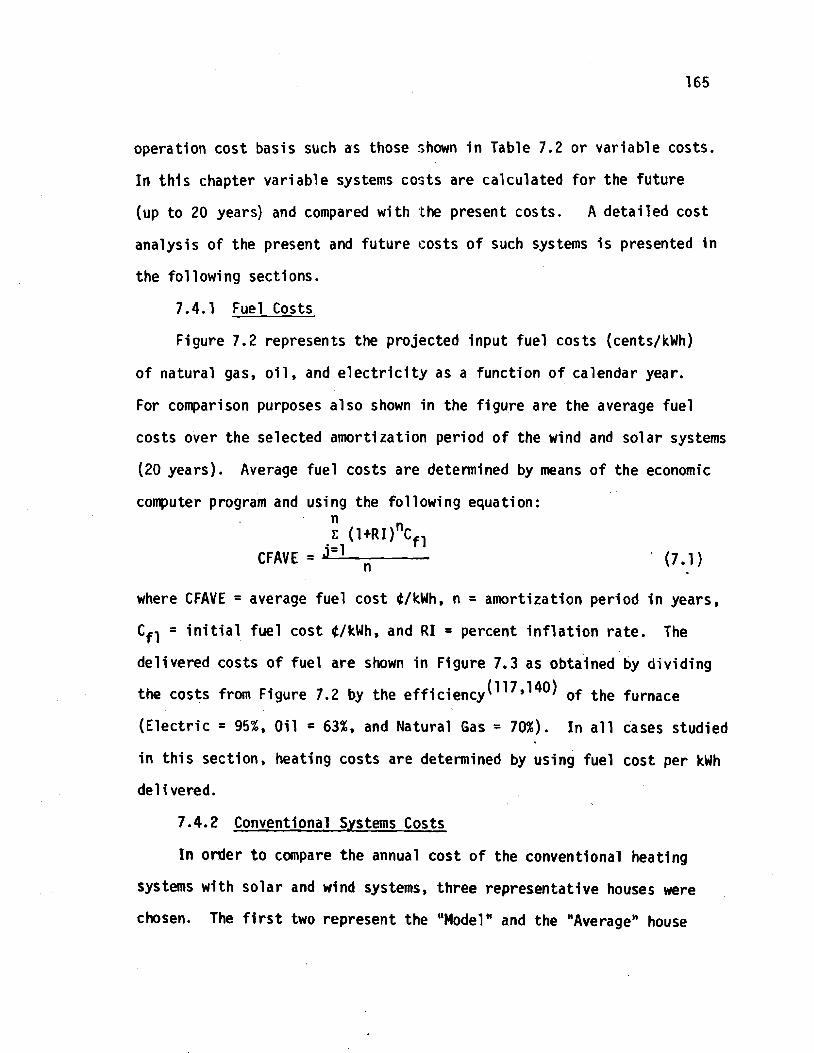
operation cost basis such as those shown i n Table 7.2 o r var iab le costs.

I n t h i s chapter var iab le systems costs are calculated f o r the f u tu re

(up t o 20 years) and compared w i th the present costs. A de ta i led cost

analysis o f the present and f u t u r e costs o f such systems i s presented i n

the f o l 1 owing sections.

7.4.1 Fuel Costs

Figure 7.2 represents the projected input f ue l costs (cents/kWh)

o f natural gas, o i l , and e l e c t r i c i t y as a funct ion o f calendar year.

For comparison purposes a lso shown i n the f i gu re are the average fue l

costs over the selected amortization per iod o f the wind and so lar systems

(20 years). Average fue l costs are determined by means o f the economic

computer program and using the fol lowing equation: n e (I+RI)~C~~

j = l CFAVE = n

where CFAVE = average fue l cost Q/kWh, n = amort izat ion per iod i n years,

Cfl = i n i t i a l f ue l cost $/kwh, and R1 = percent i n f l a t i o n ra te . The

del ivered costs o f f ue l are shown i n Figure 7.3 as ob tdned by d i v i d i ng

the costs from Figure 7.2 by the e f f i c iency( ' 179140) of the furnace

(E lec t r i c = 95%, O i l = 63%, and Natural Gas = 70%). I n a l l cases studied

i n t h i s section, heating costs are determined by using fue l cost per kwh

d e l i vered.

7.4.2 Conventional Systems Costs

I n order t o compare the annual cost o f the conventional heating

systems w i th so la r and wind systems, three representat ive houses were

chosen. The f i r s t two represent the "Model" and the "Average" house

BASIS FOR

OPERATING COST

Solar and Wind System

In t e r e s t Rate 8 Percent 1 I Amortization 20 Years

Fuel

TABLE 7.2 - Basic Economics Data Assunlptions

Inf la t ion Rate

3%

7%

4 % -

TY pe

Elec t r ic

N. Gas

Oi 1

Present Cost $/kwh

.042

.0068

.00975

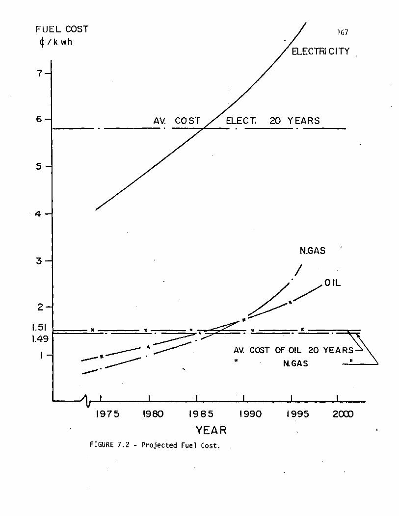
YEAR FIGURE 7 . 2 - Projected Fuel Cost.

FUEL COST 167

$ / k w h

7-

6-

5 -

4 -

3 -

2-

1.51 1.49

I -

CTRICITY .

ELECT 20 Y E A R S

N.G AS

/

AV. COST OFOIL 20 Y E A R S

-*/' .. tt N.GAS / *

t I I I I I

1975 1980 1985 1990 1995

Y E A R F I G U R E 7 .3 - Projected Fuel Cost Per kWh Delivered.

p r e v i o u s l y described, t h e t h i r d represents a t y p i c a l o l d e r home i n New

England, w i t h a much l a r g e r heat inq load. It was expected t h a t t he s o l a r

and wind heat ing o f a l a r g e r house m igh t prove t o be cos t e f f e c t i v e , s ince

energy ove r f l ow w i l l be l e s s than t h i l t o f smal le r homes. F igu re 7.4

represents the annual convent ional heat ing costs, i n do1 1 a rs l yea r , o f

the "Model" house, The y e a r l y house hea t i ng l oad i s 17,166 kwh. As

p rev ious l y discussed, i t i s very w e l l insu la ted , one s t o r y , 2 bedroom,

1500 square f e e t i n area. F igu re 7.5 shows t h e annual convent ional

heat ing c o s t o f t h e "Average" New England house w i t h a heat ing l oad o f

32,995 kwh. Th i s 1 oad a1 so represents t h e hea t i ng requirements o f t h e

UMass So la r H a b i t a t I, c o n s i s t i n g of a two bedroom res idence o f 1500

2 ft and a l a b o r a t o r y basement. The t h i r d house i s an o lder , p o o r l y

i nsu la ted , 1.5 s t o r y c o l o n i a l farm house w i t h a heat ing l oad o f 46,192

kWh/yr. The annual convent ional hea t i ng c o s t of t h i s house i s shown

i n F igu re 7.6. I n a l l t h ree f i g u r e s t h e annual cos ts a re g iven f o r th ree

types o f convent ional systems ( e l e c t r i c , o i l , and n a t u r a l gas).

As can be seen from a l l t h e r e s u l t s , the' c o s t of e l e c t r i c hea t i ng i s

s i g n i f i c a n t l y h igher than t h e c o s t of n a t u r a l gas and o i l heat ing (whose

y e a r l y cos ts a re almost i d e n t i c a l ) . Since t h e co,st of n a t u r a l gas systems

a r e a lmost i d e n t i c a l t o o i l systems costs, o n l y o i 1 and e l e c t r i c convent ional

systems w i l l be discussed i n the remainder of t h i s chapter.

7.4.3 Wind and S o l a r Systems Costs

The e f f e c t of several key system parameters on the performance o f the

wind and s o l a r systems was shown i n a prev ious chapter. One i s now i n a

p o s i t i o n t o d iscuss t h e e f f e c t of the same parameters on the t o t a l costs.

" MODEL" HOUSE

L O A D = 17166 k w h / y r

ELECT R I C/

YEAR F I G U R E 7.4 - P ro jec ted Annual Heat ing Cost o f t h e "Model" House.

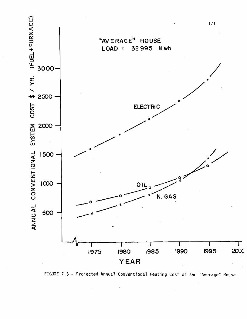
"AV E R A G E" HOUSE LOAD = 32995 K w h

/ N. GAS

Y E A R

FIGURE 7 .5 - Pro jec ted Annual Conventional Heating Cost o f t he "Average" House.

LOAD = 46192 k w h

YEAR FIGURE 7 .6 - P r o j e c t e d Annual H e a t i n g Cost o f a Large New England Home.

For example, F igure 7.7 shows the t o t a l c o s t o f t he wind system as a

f u n c t i o n o f two wind generator paramc!ters: blade diameter, and tower

he ight . As can be seen, bo th paran~elet-s i n f l uence the cos t o f the bas ic

system, w i t h b l ade diameter having a s t ronger i n f 1 uence.

F igure 7.8 presents r e s u l t s t h a t compare the t o t a l cos t o f s o l a r

on ly systems w i t h wind o n l y systems. For t h i s comparison, both wind and

s o l a r systems have a storage tank s i z e o f 2000 ga l lons . The cos t o f the

wind on ly system i s determined as a f u n c t i o n o f the blade diameter f o r

a g iven tower h e i g h t o f 60 f e e t ( t h e tower he igh t i s kept constant s ince

i t was shown e a r l i e r t h a t the performance o f t he wind system i s more

s e n s i t i v e t o the blade diameter than t o t h e tower h e i g h t ) . S i m i l a r l y ,

t h e cos t o f t he s o l a r system i s g iven as a f u n c t i o n o f the c o l l e c t o r

area ( t h e key system v a r i a b l e ) . I n the f i g u r e the so l i d 1 ines represent

present wind and s o l a r systems costs. The do t ted l i n e s represent f u t u r e

wind and s o l a r systems costs. The importance o f F igu re 7.8 l i e s i n the

f a c t t h a t f o r a s p e c i f i c t o t a l c o s t a system cou ld be chosen, then compared

on a performance basis us ing previous r e s u l t s . For example, w i t h $5000,

i n the fu tu re , one could choose e i t h e r a s o l a r system w i t h about 800

square f e e t c o l l e c t o r area o r a wind system w i t h a blade diameter o f

approximately 25 fee t . Refer ing t o t h e performance curves o f these systems

(F igure 5.10 and 5.21 r e s p e c t i v e l y ) i t i s apparent t h a t the so la r system

requ i res l ess a u x i l i a r y heat than the wind system ( f o r t he H a r t f o r d and Blue

H i l l s d a t a j .

The annual costs o f heat ing the "Average" house (32,995 kWh/yr, based

on H a r t f o r d and Blue H i l l s data) us ing wind, so la r , combined wind and so la r

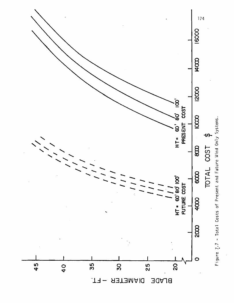
+-' c b, ffl

a r e compared nex t w i t h t h e annual hea t i ng c o s t o f t he convent ional systems.

(1) Wind Systems: Present and f u t u r e annual cos ts o f hea t i ng the

"average" house us ing wind on l y systems w i t h e i t h e r e l e c t r i c o r o i l

a u x i l i a r y a r e shown i n F igures 7.9 and 7.10 respec t i ve l y . The cos ts o f

t he wind systems a r e g iven as a f u n c t i o n o f t h e b lade diameter and f o r

a 60 f e e t tower he igh t and 2000 g a l l o n water storage tank. The f i g u r e s

a l s o show the 1975, 1995 and t h e average annual c o s t o f convent ional e l e c t r i c

and o i 1 heat ing systems. F igu re 7.9 shows t h a t bo th present and f u t u r e

annual cos ts o f t h e wind systems w i t h 25 f o o t t o 40 foo t b lade diameters

a r e l e s s than the 1975, 1995 and the average annual cos t o f t he conven-

t i o n a l e l e c t r i c hea t i ng systems. It i s a l s o shown i n F igure 7.10 t h a t

t he f u t u r e cos ts o f t he wind system, w i t h o i l a u x i l i a r y a r e l e s s than

the 1995 c o s t o f the convent ional o i l hea t i ng systems.

(2 ) Solar Systems: Present and f u t u r e annual cos ts o f heat ing the

"average" house us ing s o l a r o n l y systems w i t h e l e c t r i c o r o i l a u x i l i a r y a r e

shown i n F igures 7.11 and 7.12 r e s p e c t i v e l y . The f i gu res a l s o show the

1975, 1995 and t h e average annual cos ts of convent ional e l e c t r i c and o i l

heat ing systems. The s o l a r systems cos ts a r e presented as a f u n c t i o n of

t he c o l l e c t o r area and f o r a 2000 g a l l o n storage tank. F igu re 7.11 shows

t h a t t h e present and f u t u r e cos ts of t he s o l a r system i s much l e s s than

the 1995 convent ional e l e c t r i c systems.. It a l s o shows t h a t f u t u r e s o l a r

systems cos ts a r e approximate ly equal t o t h e 1975 e l e c t r i c convent ional

systems w h i l e the present c o s t o f t he s o l a r systems a r e s l i g h t l y h igher

i n comparing t h e s o l a r systems cos ts w i t h 1995 convent ional o i l system

cos t . F igu re 7.12 shows t h a t t h e present s o l a r systems cos ts a r e

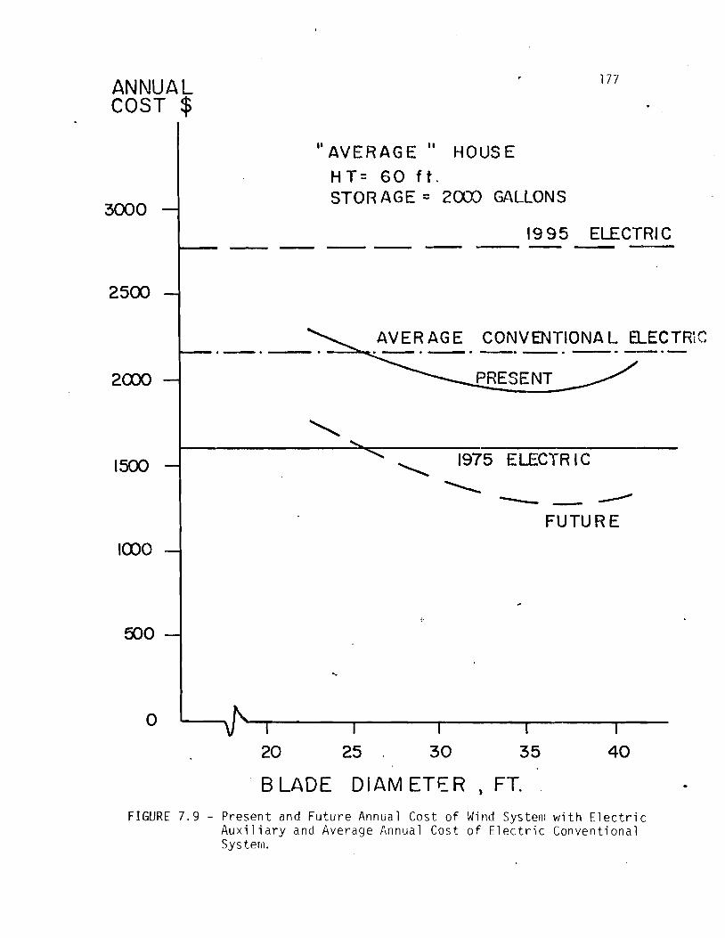
ANNUAL COST $

" A V E R A G E " HOUSE H T = 60 f t . STORAGE = 2003 GALLONS

_ _ L - -

1995 ELECTRIC --

I \ AVER AGE CONVO\ITIONA L ELECTRIC

\ 1975 ELECTRIC

\ -- / FUTU R E

BLADE DIAMETER , FT. FIGLIRE 7 .9 - Presen t and F u t u r e Annual Cost of Wind System w i t h E l e c t r i c

A u x i l i a r y and Average Annual Cost o f E l e c t r i c Conven t iona l Sys terii.

ANNUAL COST

'AVERAGE" HOUSE

H T = 60 FT.

STORAGE = 2009 GAL.

l- 1995 OIL - 'rcc FUTURE -- ---- / / . -. .-

AVERAGE CCNVENTIONAL OIL

1975 O I L

BLADE DIAMETER ,FT

F I G U R E 7.10 - Present and Future Annual Cost o f Wind System w i t h O i l A u x i l i a r y and Average Annual Cost o f O i l Conventional System

ANNUAL COST

"AVERAGE" HOUSE S T 0 RAGE = . 2000 G A L .

t-- 1995 E L E C T R lC --

F I G U R E 7.11 - Present and Future Annual Cost of Solar System with Elec t r ic Auxi 1 i a r y a n d Average Cost of E lec t r ic Conventional System.

2500 -

Xaoo-

1500 -

loo0 -

500 -

0

AVERAGE C O N V E N T I O N A L E L E C T . . - . - . . - . -.

P R E S E N T

\ \ 1 1975 ELECTRIC -

\ - - - - - FUTURE

-.

I I I 1

0 200 400 600 800

- AREA OFCOLLECTOR, f t 2

ANNUAL COST

"AVERAGE" HOUSE

S T O R A G E = 2 8 O O G A L .

200 400 a0 800

AREA OF COLLECTOR f t 2

IS00 -

Im -. 974

FIGURE 7 .12 - Presen t a n d Fu tu re Cast o f S o l a r System w i t h O i l A u x i l i a r y and Average Annual Cost o f O i l Convent iona l Sys ten^.

PRESENT

IWS O I L

FU TU FE / - - __- - . - - - .

AVERAGE CCtMVENTiONAL OIL

approxinlately equal t o the cos t o f the 1995 convent ional o i l system, wh i l e

t he f u t u r e s o l a r systenls cos ts are l ess . Also t h e r e s u l t s i n d i c a t e

t h a t both f u t u r e and present cos ts o f t he s o l a r systems a r e h ighe r than

the 1975 convent i onal o i 1 system cos t .

(3) Combined So la r and Wind Systems: The annual cos ts o f heat ing

the "Average" house (32,995 kWh/yr) us ing a combined s o l a r and wind

system w i t h e l e c t r i c , o i l , o r n a t u r a l gas a u x i l i a r y system as a f u n c t i o n

of blade diameter a re shown i n F igures 7.13 and 7.14, r e s p e c t i v e l y . Also,

the r e s u l t s present the 1975, 1995 and t h e average convent ional heat ing

system cost . The combined system cons i s t s o f a 200 square f o o t s o l a r

c o l l e c t o r , 60 f o o t tower, 2000 g a l l o n storage tank, and a v a r i a b l e blade

diameter ( t h i s system i s very much s i m i l a r t o t h e UMass So lar H a b i t a t I

except f o r t he v a r i a b l e blade d iameter ) . Present. and f u t u r e annual cos ts

a re shown and a re compared w i t h the 1975, 1995 and t h e average annual

convent ional hea t i ng cos ts o f the rep resen ta t i ve f u e l . For systems us ing

e l e c t r i c a u x i l i a r y heat i t i s shown (F igure 7.13) t h a t bo th the present

and f u t u r e s o l a r and wind systems c o s t l e s s than t h e 1995 heat ing cos t o f

a convent ional e l e c t r i c system. I t a l s o shows t h a t o n l y combined systems

w i t h a blade diameter l a r g e r than 25 f e e t and produced a t h igh volume

( f u t u r e c o s t ) w i l l compete w i t h the 1975 convent ional e l e c t r i c systems.

I t i s c l e a r from F igure 7.14 t h a t t he f u t u r e cos ts o f t h e combined s o l a r

and wind systems w i t h o i l a u x i l i a r y heat a r e l e s s than the 1995 cos t of

convent ional o i 1 hea t i ng systems.

7.5 Surr~mary o f Resul ts

F igures 7.15 and 7.16 g i v e d i f f e r e n t summaries o f t h e annual heat ing

182

" A V E R A G E " HOUSE (32,995 kw h r / y r )

TOWER HEIGHT= 60 F T STOR AGE = 2000 G A L . COLLECTOR AREA = 200 F T . ~

- FUTURE ( 1995) ELECTRIC - - --

PRESENT SOLAR + W I N D (w/ELECT. AUX

- ELECTRIC (1975)\ 1

FUTURE SOLAR + WIN D ( w / ELECT A UX. )

BLADE DIAMETER, FT.

FIGURE 7 .13 - Presen t and Fut:rre Annual Cost o f Combined S o l a r and Wind Systems w i t h E l e c t r i c A u x i l i a r y and Convent iona l E l e c t r i c Syste~ns.

ANNUAL COST

$ -- .

AVERAGE HOUSE (32,995 kwh/yr) TOWER HEIGHT = 6 0 FT. STORAGE = 2000 GAL. COLLECTOR AREA = 2 0 0 F T ~

I 1995 OIL -------- 0

0

FUTURE 4 ---------- - - - lax> . .

NERAGE CCNVE NTIONAL OIL

BLADE DIAMETER , FT.

FIGURE 7.14 - Present and Future Cost of Combined Solar and Wind . Systems with Oil Auxiliary and Conventional Oil Systems.

"AVERAGE" KXGE (32.995 k w h / yr) TOWER HEIGHT = 6 0 FT STORAGE = 2000 GAL. COLLECTOR AREA =200m2

1995 ELECTRI C t ---------- PFaESENT SOLAR +WIND + ELECT. AUX.

PRESENT 901AR + WIND + N.GAS \ AU X.

1995 N.GAS \\ FUTURE SOLAR+ WIND + ELECT AUX, -- - -\-- - - - - - - , - - , - - - - - - - - - FUTURE S+W+OILAUX. - 5 # - --.-----/ - - - # - - --

FUTURE S + W + N.GAS AUX.

BLADE.. DIAMETER ,ET.

FIGURE 7.15 - Sununary o f the Annual Heating Cost o f the Combined Solar and Wind Systems and the Fugure Annual Cost of Conventional Systems.

LOAD = 32,995 kwh H T = 6 0 FT. TANK = 2000 G A L A C O L = 200 FT.

PRESENT 0353;

AVE R . COW. ELECT.

SOLAR + WIND WlTH AUX. \\\

\ N. GAS AUX.

FUTURE CXlS'i \ SOW? +VIIND

AVE R . COW. SOLAR + WIND WlTH AUX.

ELECT.

- *\\\

\ N. GAS AUX.

FUTURE CXlS'i - 1

SOW? +VIIND

ELECT AUX. WITH AUX. ls , - - - -

ELECT AUX. WITH AUX.

a 3 - OIL AUX.-- /

,, z lox, - = = = . - <GAS AUX --

. . - - . .- GAS ( n i l

B L A D E DIA. , FT.

FIGURE 7.16 - Sununary of Present and Future Annual Cost of Combined Wind and So lar Systems and Average Annual Conventional Systenls Cost.

cos ts o f t he p rev ious l y descr ibed s o l a r and wind systems w i t h vary ing

sources o f a u x i l i a r y heat. The annual convent ional heat ing cos ts i n F igure

7.15 represents t h e 1995 expected cos ts . Whi l e t h e annual convent ional

heat ing cos ts shown i n F igure 7.16 a re the average cos ts ove r the

amor t i za t i on pe r iod of t h e s o l a r and wind systems.

The annual cos ts of s o l a r and/or wind heat ing systems w i t h e l e c t r i c

a u x i l i a r y a r e shown i n F igures 7.17, 7.18 and 7.19 as a f u n c t i o n o f t h e

a u x i l i a r y heat ing requirements of these systems. F igure 7.17 shows t h a t

f o r the "Model" house (17,166 kWhlyr) t he annual cos ts o f present, f u t u r e

s o l a r and f u t u r e wind systems are more economical than the average annual

c o s t o f the convent ional e l e c t r i c system. For t h e "Average" house (32,995

kWh/yr) and the Ranch house (46,192 kWh/yr), F igures 7.18 and 7.19

respec t i ve l y , t h e annual cos ts o f most so la r , wind, and combined s o l a r

and wind systems are c o s t compe t i t i ve w i t h t h e convent ional e l e c t r i c

system bo th a t present and f u t u r e costs.

7.6 Systems' Costs w i t h Domestic Hot Water Heat ing

It was shown i n Chapter 5 t h a t t he a d d i t i o n o f domestic h o t water

subsystem t o t h e s o l a r and/or wind hea t i ng systems does n o t reduce t h e i r

o v e r a l l performance by more than 4 percent. Therefore, i t i s now impor tan t

t o determine the e f fec t of h o t water d e l i v e r y on t h e annual c o s t o f these

systems. Since the convent ional , as w e l l as t h e s o l a r and/or wind systems,

w i l l have t h e same domestic h o t water system components (except f o r the

heat ing co71 placed i n t h e storage tank of the s o l a r and wind systems) t h e

fo l l ow ing a n a l y s i s of domestic ho t water hea t i ng cos t i s based on the

annual c o s t o f the heat ing systems p l u s the annual f u e l c o s t of domestic

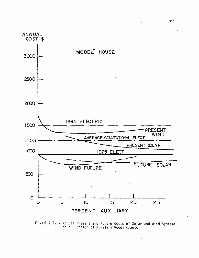
ANNUAL COST, $

1995 ELECTRIC

\\- PR ',;No'

\ AVERAGE C a d W I O N 4 L ELECT. .- PRESENT SOLAR

- 1975 ELECT. - -- / 7 --- --

WIND FUURE FUTURE SOLAR

PERCENT A U X I L I A R Y

FIGURE 7 .17 - Annual Present and Fu tu re Costs o f S o l a r and Wind Systems as a Func t i on o f A u x i l a r y Requirements.

A N N U A L COST $

"AVERAGE ' HOU SE -

1995 ELECTRIC ---- - -

AVER. CON V.

ELECT RI C

SOLAR AND WIND 1975 ELECTR lC FUTURE, 1 2 0 0 ~ ~ ~ 1 /

-

-

-

5

i I I I I 1 1

PERCENT AUXIL IARY .

FIGURE 7.18 - Annual Present and Future Costs o f So lar and Wind Systems as a Funct ion o f Auxi 1 i a r y Requi ren~ents.

1995 ELECTRIC - _ I _ - - - - - -

SOLAR & WlND PRESENT

AVERAGE C(X4VENTIONAL ELECTRIC

SOLAR+WIND

/ / FUTURE WlND

LOAD = 461 9 2 K w h / yr

I I I 1 I 1

20 SO 40 5 0 60 70

PERCENT A U X I L I A R Y FIGURE 7 .19 - Present and Future Annual Costs o f Solar and Wind Systems

as a Function o f Aux i l ia ry Requirements.

ho t wat i . : Ilea t i n g (auxi 1 i a r y o r convent ional ) . Figures 7.20 t o 7.27 present a corr~parison between t h e cos ts o f s o l a r

and wind systems w i t h 1 ) convent ional ( e l e c t r i c and o i l ) domestic h o t

water heat ing, and 2) s o l a r and wind pre-heat ing of domestic h o t water by

means o f the thermal s torage ( w i t h e l e c t r i c o r o i l a u x i l i a r y ) . The annual

c o s t o f t he s o l a r systems a re g iven as a f u n c t i o n o f area o f t h e c o l l e c t o r

2 (200 t o 800 ft ) and f o r a 2000 g a l l o n storage tank. Wind system cos ts

a re based on a v a r i a b l e b lade diameter (25 t o 40 f e e t ) , a 60 f o o t tower,

and a 2000 g a l l o n storage tank. Present and f u t u r e cos ts o f a l l systems

a re g iven f o r both t h e "Average" and "Model" houses. The annual cos ts

g iven i n F igures 7.20 t o 7.23 a re those o f s o l a r and wind systems us ing

e l e c t r i c f u e l f o r convent ional and a u x i l i a r y heat ing o f domestic h o t water.

The f i g u r e s show t h a t us ing s o l a r o r wind systems' s to rage as a pre-heat

w i l l save on the average 10 percent and 14 percent ("Average" and "Model"

houses r e s p e c t i v e l y ) o f the domestic h o t water annual heat ing c o s t compared

w i t h the convent ional ho t water heat ing. As shown i n F igures 7.21 and 7.23,

i t i s impor tan t t o no te the r a p i d increase i n savings w i t h t h e increase of

t he b lade diameter o f the wind systems (due t o the use o f the energy over-

f l o w o f these systems).

S i ~ n i l a r l y , F igures 7.24 t o 7.27 present t he annual cos ts o f s o l a r and

wind systems us ing o i l f u e l f o r convent ional and a u x i l i a r y heat ing o f

domestic ho t water. The f i gu res show t h a t us ing the s o l a r and wind thermal

s torage f o r pre-heat ing the domestic h o t water w i 11 redllce the annual heat ing

c o s t o f domestic h o t water by approximate ly 6 t o 8 percent compared w i t h

convent ional ho t water heat ing .

S O L A R H E A T I N G CON VENTION A L

H O T WATER

SOLAR H E A T I N G +

SOLAR H O T WATER

HOT WATER = 3565 K W H / Y R. " A V E R A G E " H O U S E S T O R A G E = 2000 G A L . - ELECTRI C FUEL

COLLECTOR AREA , FT.

F igu re 7.20 Annual S o l a r S y s t e m Costs w i t h Convent iona l , and S o l a r Pre-heated Domestic l i o t Water, "P.vcrafle" House.

A N N U A L COST

F i c u r e 7.21 Annual !.!ind S y s t e m Costs w i t h Convent iona l , and U ind Pre-heated Dorcestic Ho t \ !a te r , "P,veragen House.

3000

2500

2000

I500

1800

500-

- WIN D HEAT1 N G + CONVENTIONAL HOT WATER

- PRES E NT

- FUTURE \ '\

WIND HEATING + WIND HOT WATER

- '?!'& 212 - / 1

" AVERAGE" HOUSE .- HOT WATER =3565 kwh /y r

- STORAGE = 2000 GAL. HT = 6 0 FT. ELECTRI C FUEL

O + , l I I I I 20 25 3 0 3 5 4 0

B L A D E D I A M E T E R , FT

" MODEL" HOUSE HOT WATER = 3565 KWH / YR. STORAGE = 2 0 0 0 GAL. - ELECTR I C FUEL

SOLAR HEATING

- + CONVENTIONAL

- / -- / FUTURE

SOLAR HEATING + SOLAR HOT WATER

0 I I 1 I I

200 400 600 800 1000

COLLECTOR A R E A , FT*

F i g u r e 7.22 Annual So la r Systems Costs w i t h Convent iona l , and S o l a r Preheated Domestic Ho t Water, "Model" Hcuse.

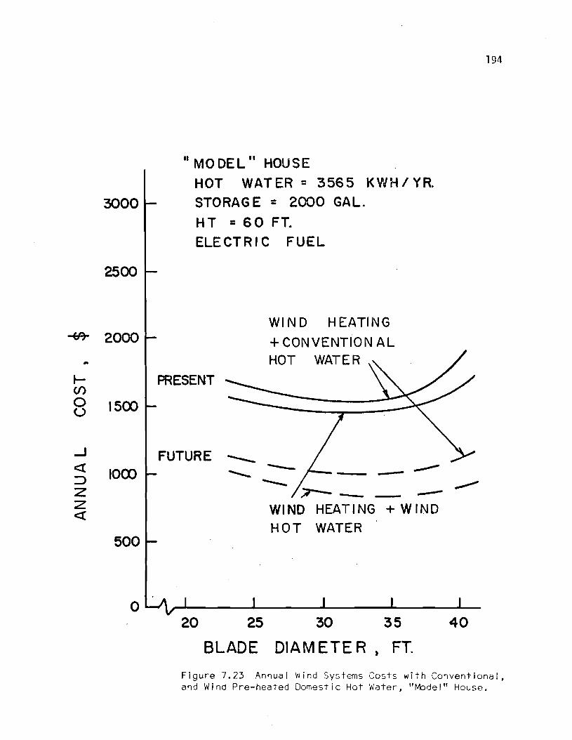
" MODEL" HOUSE HOT WATER = 3565 KVdH/YR.

- STORAGE = 2000 GAL.

H T = 6 0 FT. ELECTRIC FUEL

WIND HEATING + CONVENTI'ON AL HOT WATER

PRESENT

-

FUTURE 1 - -- /

WIND HEATING + WIND HOT WATER -

BLADE DIAMETER , FT.

F i g u r e 7.23 Annual Wind Systems Costs wi:h Convent iona l , and Wind Pre-heated Domest ic Ho t Water, "Model" House.

" A V E R A G E " HOUSE

HOT WATER = 3 5 6 5 K W H / Y R . STORAGE = 2000 GAL O I L F U E L

SOLAR HEATING + CONVENTIONAL

HOT WATER

/ - - - - - - - T\

_-. - - - FUTU RE

S O L A R HEATING +

I SOLAR HOT WATER

F i c u r e 7.24 Anru:.l Ccst- of Sc l a r Sysf-cr is w i i - 1 1 Cor~~ /en t ion<z I , 9. an3 Colar Pre-hea lei l j o r r e s t i c Hct ';:ate.r-, "Averaqe" - l:f-'tj;e.

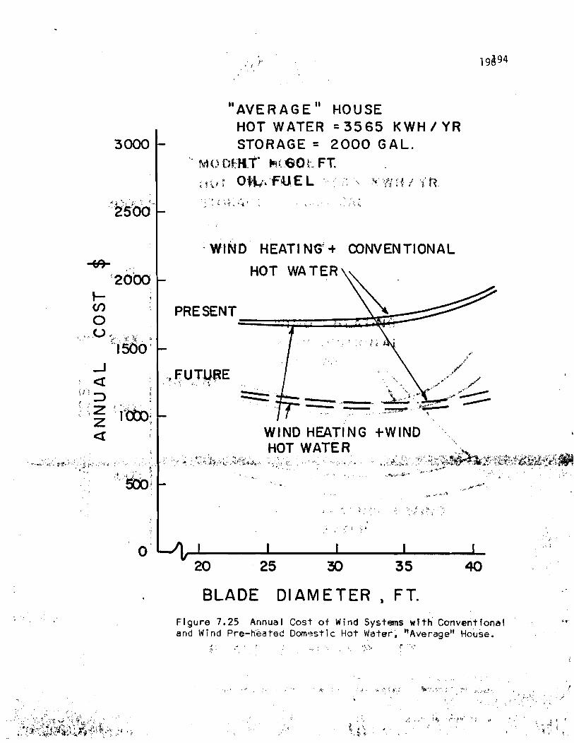
" A V E R A G E " HOUSE HOT WATER =3565 K W H / Y R STORAGE = 2 0 0 0 GAL.

" ed r s ~ ~ f . ) d f ' hi 6 0 4. FT : t ; * : O$$& FUEL - ', , r :";':{ I; f t 3

t , L I " " % a # . . < ' ' I L

- WIND' HEAT1 NG + CONVENTIONAL

HOT WATER\\ -

PRESENT A

WIND HEATING +WIND " - . I

HOT W ATE R ' . , . .x <i.. ; '.

r ' .* . . ,..&;*+* $3,;,(' .. ,;- .',.7:5.*4: - * ..~" .:., , i , , . . : ',. . . . " l . . : ; . ,'. , , , .IJ.-~.:; - , . , . ,,?. . . !,**:.~,~L~?.;x + . .., $&,"'. 7 ,, ,*.. */..; i; . &q;,~<~&&?%~ipi4&~,# s"', ,: ,,. .: .;* '%* pC6. ..,. ,. 1

, ." ..,*-.* . . < " ... . " , . . , , ,a*,.. -$.' z .' . .

.w *a

.4 * -7

BLADE D I A M E T E R , FT. F i g u r e 7.25 Annual Cost o f Wind Systems with Conventional .I and Wind P r e - b a t e d D m s s t i c Hot Water, " ~ v e r a g e " House.

. I i . 'a 1, * . I

I u MODEL" HOUSE HOT WATER = 3565 M W H / Y R . S T O R A G E = 2000 G A L . O I L FUEL

SOLAR HEATIN5 + CONVENTIONAL PREsmT H O T WATER

-- c-

SOLAR HEATING -+ SOLAR HOT WATER

F i g u r e 7.26 Annuai Ccst o f S o l a r Systems w i t h Ccnvcnt i o n a l , and S o l a r Pre-heated Domest ic H o t Wate~ ' , "Average" House.

" MODEL " HOU S E HCK WATER = 3565 KWH/YR. STORAGE = 2 0 0 0 GALLONS

HT = 60 FT. O I L F U E L

- WIND HEATING 9 CONVENTIONAL

HOT WATER

WIND HEATING + WIND 500 HOT WATER

0 I I I I

0 20 25 30 35 40

BLADE D IAM ETE R , FT.

F i g u r e 7.27 Annual Cost o f Nind Systems w i t h Conventional, and W i n d Pre-heated Gorrest i c Hot- Xat e! - , "klcde I " t iouss.

C H A P T E R 8

CONCLUSIONS AND RECOMMENDATIONS

A detailed discussion of solar and/or wind systems performance

and economics were presented in Chapters 5 , 6, and 7. I n t h i s Chapter

conclusions based on this study and recommendations for future studies

related t o wind, solar , and combined wind and solar systems will be made.

8.1 Conclusions '

Based on the previous resul ts , the following conclusions are divided

into two categories: A ) Performance, and B ) Economics.

A. Performance:

1. Wind systems performance i s more sensitive t o blade diameter

than the tower height.

2. An optimum storage size could be determined for a specific system

configuration for both wind and combined wind and solar systems.

3 . When a minimum baseboard heater s ize for a system i s reached a

larger s ize does not significantly improve i t s performance.

4 . A wind system corresponding to current UMass f ac i l i t y (D=32.5 f t ,

HT=60 f t , H.X.=50 f t , and 2000 gallon storage) will provide over 75 percent

of the heating requirements of an "Average" New England house, and a l l

the heating load of a "Mgdel" house (very we1 1 insulated).

2 5. A solar system with a vertically mounted collector (ACOL=800 f t ,

H. X.=50 f t , and 2000 gallon storage) wi 11 supply over 60 percent of the

"model " house heating requirements.

6. The performance of the combined wind and solar systems i s more

sensitive t o percentage changes in the s ize of wind generator blade than

the s ize of the collector.

. . SO0

7. Separat ing wind and s o l a r s to rage i n t o two tanks f o r t he

corr~bined wind and s o l a r systems w i l l inc rease t h e systems performance

by approximately one percent f o r l a r g e r systems and decrease the per -

formance by approximate ly one percent f o r smal l e r sys terns.

8. Using s o l a r and wind systems s torage as a -p rehea t f o r domestic

h o t water w i l l decrease t h e o v e r a l l performance o f these systenis by

approximate ly (2 t o 4) percent and supply 40 t o 97 percent (depending on

t h e type and component s i z e o f t h e systems) o f the domestic h o t water

hea t i ng requirements.

6. Economics

1. Wind systems' cos ts a re more s e n s i t i v e t o b lade diameter s i z e

than tower he igh t .

2. Present and f u t u r e wind systems' costs a re c o s t compe t i t i ve

w i t h e l e c t r i c convent ional hea t i ng systems,

3. Future s o l a r systems' cos ts a re cos t compe t i t i ve w i t h 1975

e l e c t r i c convent ional hea t i ng systems.

4. Present s o l a r systems' cos ts a re c o s t e f f e c t i v e when compared

t o e l e c t r i c convent ional hea t i ng systems over 20 years amor t i za t i on

per iod .

5. A t present s o l a r systems are n o t c o s t con~pet i t i v e w i t h conven

t i o n a l o i l o r n a t u r a l gas hea t i ng systems.

6. Combined s o l a r and wind systems are cos t compe t i t i ve w i t h con-

vent iona l e l e c t r i c a t 1975 p r i ces .

7. . Most s o l a r and wind systenis a re cos t e f f e c t i v e when compared t o

convent ional e l e c t r i c hea t i ng a t 1975 p r i ces .

8. Most s o l a r and wind systems would be cos t e f f e c t i v e over 20

years amor t i za t i on per iod.

9. Using s o l a r and wind systems as preheat f o r domestic h o t

water reduces the annual h o t water heat ing c o s t by 40 t o 90 percent

compared t o convent ional h o t water heat ing.

8.2 Recomrnendations f o r Future S tud ies

I n t h e near f u t u r e wind and s o l a r energy cou ld produce a consider-

ab le p o r t i o n o f t he Uni ted States and t h e wor ld ' s space heat ing energy.

Therefore, t h i s s tudy and f u t u r e s tud ies w i l l p l a y an impor tant r o l l i n

improving the performance o f these systems and increas ing t h e i r d e s i r -

a b i l i t y . It i s f e l t t h a t t he re are a number o f areas t h a t need f u r t h e r

i n v e s t i g a t i o n and ana lys i s i n the f u t u r e such as:

1. The need f o r experimental v e r t i f i c a t i o n o f model by us ing So lar

H a b i t a t da ta (33) and should i nc lude c a l i b r a t i o n o f i n d i v i d u a l component

model s . 2. Add i t i ona l a n a l y t i c a l runs us ing o the r designs f o r wind generator

components ( i .e. changes i n t h e performance o f t he present design o r

t o t a l l y a new generator) . A lso i nc lude the e f f e c t s o f f u r t h e r improve-

ments on t h e wind generator economics.

3. Expand s tud ies t o i nc lude mu1 t i - f a m i l y residences, i n s t i t u t i o n a l , and farm heat ing app l i ca t i ons . Large w indmi l l a r rays w i l l obv ious ly be

needed f o r such appl i c a t i ons . 4. Continue s i n g l e f a m i l y s tud ies t o i nc lude o t h e r s i t e s (as new

h o u r l y wind and s o l a r data i s accumulated).

5 . Develop a s i m p l i f i e d design procedure, such as was developed f o r

s o l a r on ly systems by K le in , e t a1 . (52, 42) f o r t he wind and t h e com-

b ined wind and s o l a r systems. Such a procedure would e l i m i n a t e t h e use

of hour-by-hour data and the d e t a i l e d c a l c u l a t i o n procedure.

6. Expand the econonlic s tudy t o i n c l u d e such f a c t o r s as increased

amor t iza t ion per iod, reduced i n t e r e s t ra tes , t a x i ncen t i ves , e t c .

7 . Expand modeling t o i n c l u d e systems t h a t supply e l e c t r i c i t y on

demand ( o r w i t h some e l e c t r i c a l storage) from t h e wind generator. Such

systems could use h igh temperature thermal s torage w i t h a Rankine c y c l e

r e c y c l i n g t o a low temperature storage ( t o be used f o r r e s i d e n t i a l heat ing) .

8. Consider o ther v a r i a t i o n s o f conventional heat ing systems such

as heat pumps.

9. Determine cos t advantage o f b u i l d i n g s o l a r and wind systems as

p a r t o f the b u i l d i n g s t r u c t u r e .

10. Develop a break-even model o f s o l a r and wind systenis' costs

compared t o conventional heat ing sys tems . 11. Consider i n d e t a i l s market capture and consumer acceptance of

s o l a r and wind heat ing systems.

REFERENCES

Solar Heating and Cool ing of Bu i ld ings , General E l e c t r i c Co., N.S.F., May 1974, Vol. 111.

Glaser, Peter E. , "The Case o f So lar Energy," ~ F t h u r D. L i t t l e , Inc., Sept. 3, 1972.

Br idgers, Frank H. , "Applying So lar Energy f o r Cool ing and Heating I n s t i t u t i o n a l Bui ld ings," ASHRAE Journal, Sept. 1974.

Roberts, Ralph, "Energy Sources and Conversion Techniques, " American S c i e n t i s t , 1966, Vol. 61.

"Resident ia l Water Heating:. Fuel Conservation Economical and Pub1 i c Pol icy," N.S.F. by J.J. Mutch, R-1498-NSF, May 1974.

Heronemus, W . E. , "A1 t e r n a t i v e Energy Resources t h a t Should I n t e r e s t ' the U.S. Navy," U.S. Navy Energy Symposium U.S.N.R. DC, Annapolis, 14aryland, Sept. 18, 1973.

Steadman, P h i l i p , "Energy, Environment and Bui ld ing," Cambridge U n i v e r s i t y Press, Cambridge, England, 1975.

",Solar Heating and Cool ing of Bui ld ings," TRW System Group, TRW Report No. 25168.001, May 31, 1974, C a l i f o r n i a .

"An Assessment of So lar Energy as a Nat ional Energy Resource," IdSF/NASA So lar Energy Panel , December 1972.

"Solar Heating and Cool ing of Bui ldings," General E l e c t r i c Co., N.S.F., May 1974, Vol. I .

"Solar Heating and Cool in.g of Bui ld ings," General E l e c t r i c Co., N.S.F., May 1974, Vol. 11.

Lof , G.O. and Tybout, R.A., "A Model fo r op t im iz ing So lar Heating Design," ASME 72-WA/SOL-8.

Tybout, R.A. and Lof , G.O. , "Solar House Heating," Natura l Resources Journal, Vol. 10, 268 (1970).

14. Lof, G.O. and Tybout, R.A., "The Design and Cost of Optimized Systems f o r Cool ing Dwell ings by Solar Energy," Paper presented a t the I n t e r n a t i o n a l So lar Energy Soc ie ty Congress, Par is (1 973).

15. Lof , G.O. and Tybout, R.A., "Cost of House Heating w i t h Solar Energy," So lar Energy, - 14, 253 (1973).

Pete rs , Warren D. , "A D e t a i l e d Study o f New England R e s i d e n t i a l H e a t i n g Systems U s i n g S o l a r Energy and Heat Pumps," Mas te r o f Sc ience P r o j e c t Repor t , Dept . o f Mechanical Eng ineer ing , U n i v e r s i t y o f Massachuset ts , Amherst, 1974.

Balcomb, D., e t a l , " S o l a r H e a t i n g Handbook f o r Los Alamos," LA-5967, Los Alamos S c i e n t i f i c Labora to ry , Los A1 amos, New Mexico, 1975.

Ward, Dan S., "Performance o f a R e s i d e n t i a l S o l a r H e a t i n g and C o o l i n g System," Annual Progress Repor t , 711174-2/1/75, Colorado S t a t e U n i v e r s i t y .

Proceedings o f t h e S o l a r H e a t i n g and C o o l i n g f o r B u i l d i n g Workshop, NSF, NTIS PB 223-536, 1974.

B e t t i g n i e s , C . , " P o t e n t i a l o f Windpower U t i l i z a t i o n i n t h e A r c t i c Environment, House Heat ing, " Brace Research I n s t i t u t e P u b l i c a t i o n DT-8, August 1970.

Ga lan is , N. and D e l i s l e , A., "Performance E v a l u a t i o n o f Wind D r i v e n eati in^ Systems," Proceedings o f 8 t h I n t e r s o c i e t y Energy Convers ion E n g i n e e r i n g Conference, 1973.

" S o l a r Energy f r o m Ear th , " an AIAA Assessment, American I n s t i t u t e o f A e r o n a u t i c s and A s t r o n a u t i c s , New York, A p r i 1 21 , 1975.

E l d r i d g e , F.R., "Wind Machines," The MITRE C o r p o r a t i o n , MTR-6971, NSF-RA-N-75-051, October 1975.

S i s k i n d , C h a r l e s S., " E l e c t r i c a l Machines, D i r e c t and A l t e r n a t e C u r r e n t ," 2nd E d i t i o n , McGraw-Hi1 1 . 1959.

G l a u e r t , H., -- Elements o f A e r o f o i l and A i r s c r e w Theory, Cambridge U n i v e r s i t y Press, 1959.

Gold ing, E.W., "The Genera t ion o f E l e c t r i c i t y by Wind Power," P h i l o s o p h i c a l L i b r a r y , New York, 1956.

S o l a r R a d i a t i o n Data a t S o l a r House I V , B lue H i l l s , Massachusetts, 1959.

W h i l l i e r , A., "Notes on S o l a r Energy," Brace Research I n s t i t u t e o f M c G i l l U n i v e r s i t y , T e c h n i c a l Repor t No. T.63, Oct . 1964, Quebec, Can.

29. H o t t e l , H.C. , and Woertz, B. B. , "The Performance of a F l a t - P l a t e S o l a r Heat C a l l e c t o r , " T r a n s a c t i o n o f t h e A.S.M.E., 64, P. 91 (February 1942).

30. " R e s i d e n t i a l Hot Water S o l a r Energy S to rage Subsystems," S t a n f o r d Research I n s t i t u t e , T e c h n i c a l Repor t , PB252685, NSF RA-N-75-095, January 1976.

Johnson, C .A. , "Engineering S t r u c t u r a l Modules f o r Economical Housing," American Society o f A g r i c u l t u r a l Engineers, Paper No. 72- 91 0, December 1972.

Corman, J.C., McGowan, J.G., and Peters, W.D., "Solar Augmented Hone I ieat ing Heat Purnp System," Proceedings of the 9 t h I n t e r - soc ie ty Energy Conversion Engineering Conference, 1974.

Wells, W.D., "Design and I n s t a l l a t i o n o f a Heating System f o r a Solar and Windpower Heated Home," Master o f Science Pro jec t , ME, U n i v e r s i t y o f Massachusetts, Amherst, MA, August 1976.

ASHRAE Handbook o f Fundamentals, American Society o f Heating, Re f r ige ra t ion , and A i r Cond i t ion ing Engineers, ASHRAE Publ ica t ion , 1972.

K re i th , Frank, P r i n c i p l e s o f Heat Transfer, - I n t e r n a t i o n a l Textbook Company, 5 t h p r i n t i n g , June 1969.

Schl i c h t i n g , H., "Boundary Layer Theory," 6 t h Ed i t i on , McGraw-Hi 11 , 1 968.

Kays, W. and London, A.L., Compact Heat Exchangers, 2nd Ed i t i on , McGraw-Hi 11, 1964.

Westinghouse E l e c t r i c Corporat ion, "Solar Heat ing and Cool i n g o f Bui ld ings, Phase 0," F i n a l Report, Volume I, PI3 235-427, May 1974.

Westinghouse E l e c t r i c Corporation, "Solar Heating and Cool ing o f Bu i ld - ings, Phase 0," F ina l Report, Volume 11, PB 235 428, May 1974.

Westi nghouse E l e c t r i c Corporat ion, "Solar Heating and Cool ing o f .Bu i l d ings , Phase 0," F ina l Report, Volume 111, PB 253 429, May 1974.

TRW System Group, "Solar Heating and Cool ing o f Bui ldings," TRW No. 25168.002, Volume 11, May 1974.

TRW System Group, "So lar Heating and Cooling. o f Bui ldings," TRW No. 25168.003, Volume 111, May 1974.

NSF/NASA, "Wind Energy Conversion System," Workshop Proceedings, NSF/RA/N-73-006, December 1973.

Du f f i e , J.A.9 e t a l . , Semi-Annual Progress Report, January 1974, NTIS No. PB 2441 51 .

Nat ional Bureau o f Standards, "Solar Heating and Cooling o f Bu i ld ings: Methods of Economic Evaluat ion," U.S. Department of Corrmerce, NTIS No. Com-75-11070, J u l y 1975.

46. Chan, D.C. , "Res ident ia l Energy Consumption and Small-Scale Options o f Energy Systems f o r Space Heating," MITRE Technical Report MTR-2951, November 1974.

47. U n i v e r s i t y o f Massachusetts, " I n v e s t i g a t i o n o f t he F e a s i b i l i t y o f Using Windpower f o r Space Heating i n Colder Cl imates," T h i r d Q u a r t e r l y Report Uiilass., Archerst, Report NO. NSF/RANN/AER-75- 00603/PR/75/3, December 1975.

48. A1 t e r n a t i v e Sources o f Energy, ASE's Spectrum, An A1 t e r n a t i ve Technical Equipment D i r e c t o r , Route 2, Box 90A, Mi laca, MN 56353.

49. Massdesign, A r c h i t e c t s and Planners, Inc. , "Solar Heated Homes f o r New England," Cambridge, Mass. , A p r i l 1975.

50. Heronemus, W.E., Professor, Personal Communication, January 1974, Department o f C i v i l Engineering, Uni vers'i t y o f Massachusetts, Amherst, MA 01003.

51. K le in , S.A. , Beckman, W.A., and D u f f i e , J.A., "A Design Procedure f o r Solar Heat ing Systems," So lar Energy, Volume 18, No. 2, 43 (1976).

52. K le in , S.A. , Beckman, W.A., and D u f f i e , J.A., "A Design Procedure f o r Solar A i r Heat ing Systems," Proceedings o f t h e I n t e r n a t i o n a l So lar Energy Soc ie ty Conference, Volume 4, 1976.

APPENDIX A

NOMENCLATURE

A : Area swept by the r o t o r

Aa : Solar a1 ti tude angle

A,, ACOL: Area o f t h e s o l a r c o l l e c t o r

ACON : Annual c o s t of the conventional system

ACS : Annual system c o s t

A r : I n i t i a l c o s t charged f o r any s i z e r o t o r

As : Storage tank surface area

Awi n : Area o f t he windows

B : Surface t i lt angle, from the sur face t o the h o r i z o n t a l

C : M u l t i p l i c a t i o n factor , f u n c t i o n o f t i lt angle

'AF

' a i r

CAUX :

C1

Auxi 1 i a r y furnace c o s t

Spec'if ic heat o f a i r

Annual a u x i l i a r y f u e l cos t

S p e c i f i c heat o f c o l l e c t o r absorber p l a t e

Cost o f frame and t ransmission

Cloud cover on sca le 0 - 10, (O=clear, 1 O = f u l l c loud cover)

Cold f l u i d capac i ty r a t e

Cost o f so l a r c o l l e c t o r

C o l l e c t o r cos t per u n i t area

Cost o f heat de l i v e r y system

Annual conventional fuel cos t

degrees

ft2

ft2

ft2

degrees

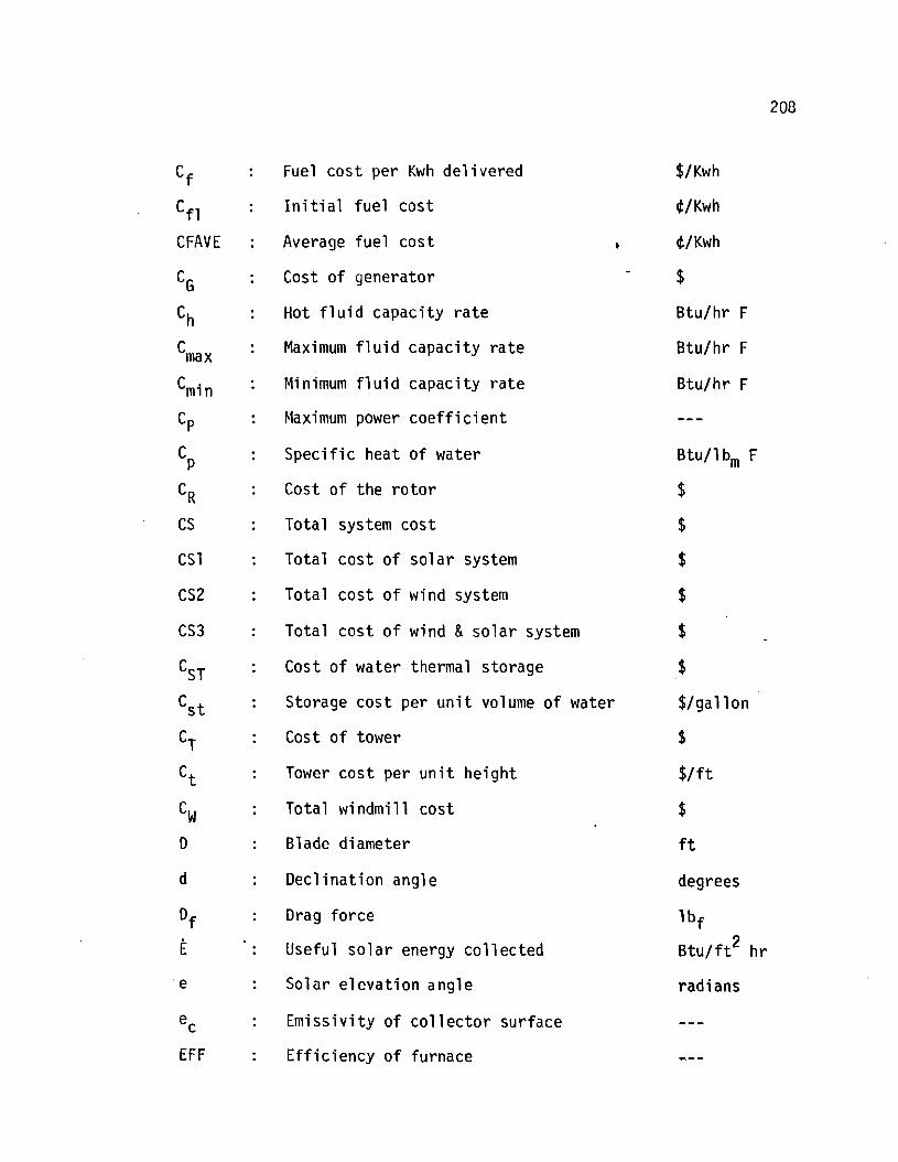
Fuel cos t per Kwh delivered

I n i t i a l fuel cost

Average fuel cost + CFAVE

Cost of generator

Hot f l u id capacity r a t e

Maximum f lu id capacity r a t e

Minimum f lu id capacity r a t e

Maximum power coef f ic ien t

Specific heat of water

Cost of the ro tor

Total system cost

Total cos t of so la r system

Total cos t of wind system

Total cos t of wind & so l a r system

Cost of water thermal storage

Storage cos t per u n i t volume of water

Cost of tower

$/gal lon

$

$ / f t Tower cos t per uni t height

Total windmill cost

Blade diameter

Decl ination angle degrees

bf

s t u / f t 2 h r

Drag force

Useful so l a r energy coll ected

Solar elevation angle

Emissivity of co l lec tor surface

Efficiency of furnace

radians

c

EFF

Emiss i v i t y o f g l a z i n g

Force a c t i n g on blades

Hour angle o f the sun, noon = 0, af ternoon = p o s i t i v e

degrees

Convective heat t r a n s f e r c o e f f i c i e n t

Convective heat t r a n s f e r c o e f f i c i e n t between two para1 1 e l ti 1 ted p la tes

I n s i d e h . t . convect ive c o e f f i c i e n t

Outside h . t . convect ive c o e f f i c i e n t

Windmil l tower he igh t

Length o f baseboard heaters

Tota l s o l a r i n s o l a t i o n on a v e r t i c a l sur face

So lar inc idence angle on a v e r t i c a l sur face

degrees

Solar inc idence angle on a t i l t e d sur face

degrees

D i r e c t s o l a r r a d i a t i o n on a v e r t i c a l sur face

D i r e c t s o l a r r a d i a t i o n on a t i l t e d sur face

Percent i n t e r e s t r a t e

D i f f used s o l a r r a d i a t i o n

Mu1 t i p 1 i c a t i o n constant

Rat io o f drag t o l i f t fo rce

Thermal c o n d u c t i v i t y o f a i r

K i n e t i c energy o f wind

Thermal c o n d u c t i v i t y o f storage tank wa l l s

L a t i t u d e degrees

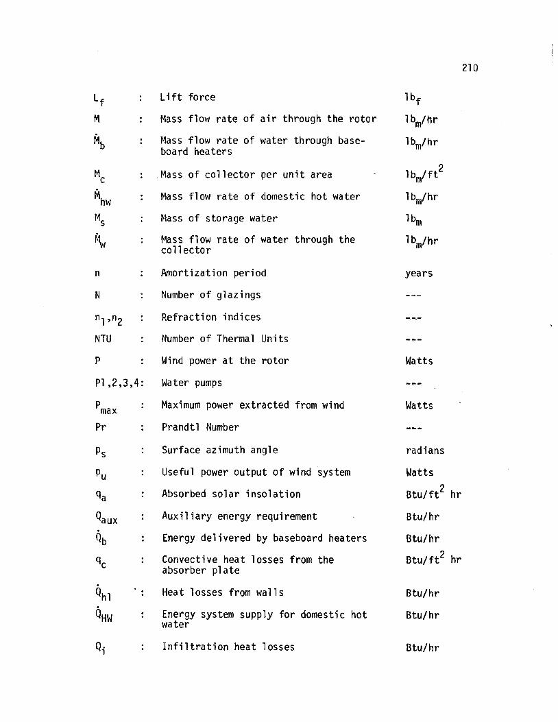
Lift force

Mass flow rate of a i r through the rotor

Mass flow ra te of water through base- board heaters

Mass of collector per unit area

Mass flow rate of domestic hot water

Mass of storage water

Mass flow rate of water through the coll ector

Amortization period years

Number of glazings

Refraction indices

Number of Thermal Units

" 1'" :

NTU

Wind power a t the rotor Watts

Water pumps

Maximum power extracted from wind Watts

Prandtl Number

p s

p u

9 a

Qaux

4 b

c

Surface azimuth angle radians

Useful power output of wind system Watts

~ t u / f t ~ hr Absorbed solar insolation

Auxiliary energy requirement

Energy delivered by baseboard heaters

Convective heat losses from the absorber p l a t e

Heat 1 osses from wall s

Energy system supply for domestic hot water

Inf i l t ra t ion heat losses

Heat losses from the co l lec tor

Maxiniurn energy delivered by baseboard heaters

Net home heating load

Useful so la r energy col l ected

Energy change of storage tank

Transmitted s o l a r radia t ion through the glazings

Heat losses from storage walls

Total heating load

it 1

Qtotal ' Qw

Q w i n

Useful wind energy

Solar energy transmitted t o the house through windows

Fixed amortization r a t e

Refraction angle degrees

Fraction ref lacted of d i r e c t so la r insolat ion

Rex

R I

R~

Reynold's Number based on length

Percent in f la t ion r a t e

Fraction of d i r e c t so l a r insolat ion ref lacted due t o N covers

Fraction ref lacted of diffused s o l a r radiation

SHADE : Shading fac tor fo r windows and col 1 ec tor

Thrust of the rotor

Time

Ambient temperature

Model 3-0 wind storage tank

Model 3-8 so la r storage tank

Water i n l e t and e x i t temperature o f baseboard heaters

Cold f l u i d ten~perature o f t he heat exchanger

Cold water temperature fro111 t h e main -

D r i v i n g f o r c e on blades

Teniperature o f f i r s t & second g laz ings r e s p e c t i v e l y

Storage tank w a l l s th ickness f e e t

F Hot f l u i d temperature o f t h e heat exchanger

Water i n l e t and e x i t temperature o f t he c o l l e c t o r

Temperature o f t he c o l l e c t o r p l a t e

C o l l e c t o r p l a t e temperature a t beginning and end of t he hour

Room temperature

Temperature o f s torage

Water temperature through the c o l l e c t o r

Storage tank o v e r a l l heat t r a n s f e r c o e f f i c i e n t

Wind v e l o c i t y a t t he r o t o r mph

mph

mp h

f t 3 / h r

m/sec

mph

mph

ga l 1 ons

Tangent ia l wind v e l o c i t y

Upstream and downstream wind v e l o c i t i e s

Volumetr ic i n f i l t r a t i o n r a t e

W i nd ve l o c i t y i n meter per second

Wind r e l a t i v e v e l o c i t y

Wind speed a t s f e e t above ground

Volume of water i n s torage

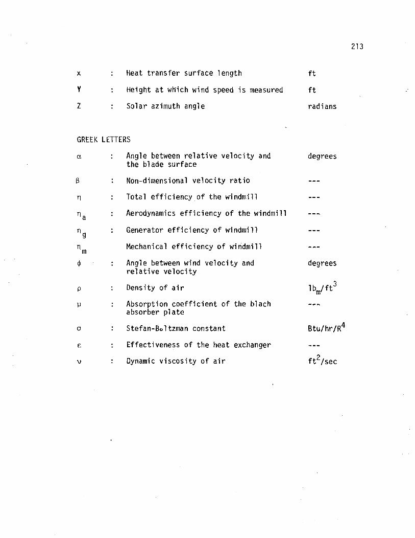
x : Heat t r a n s f e r sur face leng th

Y : Height a t which wind speed i s measured

Z : Solar azimuth angle

GREEK LETTERS

a : Angle between r e l a t i v e v e l o c i t y and t h e b lade surface

B : Non-dimensional v e l o c i t y r a t i o

n : Tota l e f f i c i e n c y o f t h e w indmi l l

na : Aerodynamics e f f i c i e n c y o f t h e windmi 11

n : Generator e f f i c i e n c y o f windmi 11 9

'rn Mechanical e f f i c i ency o f w indmi l l

4 : Angle between wind v e l o c i t y and re1 a t i v e v e l o c i t y

P : Densi ty of a i r

1.1 : Absorpt ion c o e f f i c i e n t of t he b lach absorber p l a t e

a : Stefan-Boltzman constant

E : Effect iveness o f t h e heat exchanger

v : Dynamic v i s c o s i t y o f a i r

ft

ft

radians

degrees

- -- degrees

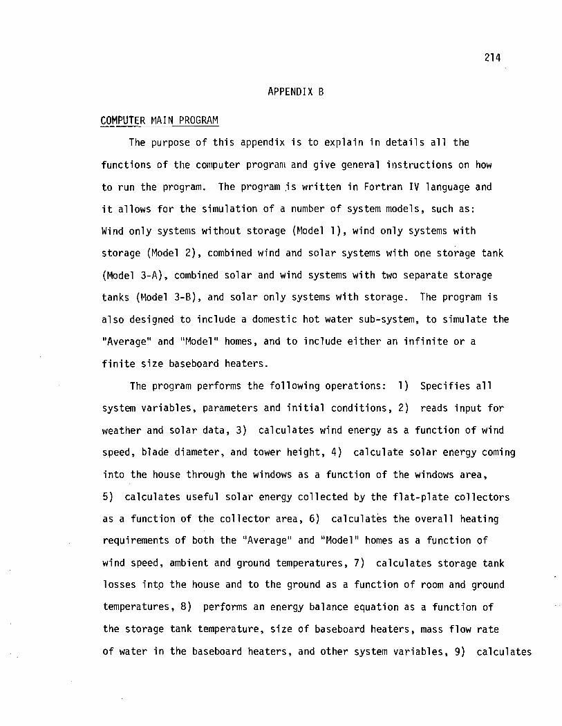
APPENDIX B

COMPUTER MA1 N PROGRAM

The purpose o f t h i s appendix i s t o exp la in i n d e t a i l s a l l t he

func t i ons o f t h e cotriputer program and g i v e general i t ~ s t r u c t i o n s on how

t o r u n the program. The program . is w r i t t e n i n For t ran I V language and

i t al lows f o r t h e s imu la t i on of a number o f system models, such as:

Wind o n l y systems w i thou t s torage (Model I ) , wind o n l y systems w i t h

storage (Model 2), combined wind and s o l a r systems w i t h one storage tank

(Model 3-A), combined s o l a r and wind systems w i t h two separate storage

tanks (Model 3-B), and s o l a r o n l y systems w i t h storage. The program i s

a l s o designed t o i nc lude a domestic h o t water sub-system, t o s imulate t h e

"Average" and "Model" homes, and t o i nc lude e i t h e r an i n f i n i t e o r a

f i n i t e s i z e baseboard heaters.

The program performs t h e f o l l owing operat ions: 1 ) Spec i f i es a1 1

system var iab les , parameters and i n i t i a l cond i t ions , 2) reads i n p u t f o r

weather and s o l a r data, 3) ca l cu la tes wind energy as a f u n c t i o n o f wind

speed, blade diameter, and tower he ight , 4 ) c a l c u l a t e s o l a r energy coming

i n t o t h e house through t h e windows as a f u n c t i o n o f t he windows area,

5 ) ca l cu la tes usefu l s o l a r energy c o l l e c t e d by t h e f l a t - p l a t e c o l l e c t o r s

as a f u n c t i o n o f t h e c o l l e c t o r area, 6) ca l cu la tes t h e o v e r a l l heat ing

requirements o f both t h e "Average" and "Model" homes as a f u n c t i o n o f

wind speed, ambient and ground temperatures, 7 ) ca lcu la tes storage tank

losses i n t o t h e house and t o t h e ground as a f u n c t i o n o f room and ground

temperatures, 8) performs an energy balance equat ion as a f u n c t i o n o f

t h e storage tank temperature, s i z e of baseboard heaters, mass f l o w r a t e

o f water i n t h e baseboard heaters, and o the r system var iab les , 9 ) ca l cu la tes

domest ic h o t water energy requi rements as a f u n c t i o n o f t h e s to rage

tank temperature, 10) c a l c u l a t e s t h e system energy o v e r f l o w and

a u x i l i a r y energy requi re~: icnts f o r space h e a t i n g and do~ i i es t i c h o t water ,

11) c a l c u l a t e s new i n i t i a l c o n d i t i o n s o f t h e systeni, 12) o u t p u t

i nc l udes hou r l y , d a i l y , month ly and y e a r l y r e s u l t s .

INPUT

Data i n p u t t o t h e program i s d i v i d e d i n t o s i x da ta banks (B1, B2,

B3, B4, B5 and B6) . Each da ta bank covers a p e r i o d o f two months

s t a r t i n g w i t h September and October (B1). Data i s g i v e n i n h o u r l y

measurements o f t h e f o l l o w i n g : S o l a r i n s o l a t u i o n (SUN), c l o u d cover

(CC) measured on a 0 t o 10 sca le , where 0 equals c l e a r sky and 10

comp le te l y overcas t , Wind speed ( N V ) , d r y b u l b a i r temperature (NTA) ,

and wind d i r e c t i o n (WD) i n tens o f degrees measured f rom due no r th , where

09 = East, 18 = South, 27 = West, 36 = No r th and 00 = calm. A sample o f

one day o f data, 24 hours, i s shown i n F i g u r e B.1.

DOMESTIC HOT WATER SUBROUTINE -

This sub rou t i ne c a l c u l a t e s t h e D.H.W. energy requi rements, energy

suppl i e d by t h e s o l a r and/or wind systems f o r D.H.W. hea t ing , and t h e

a u x i l i a r y hea t r e q u i r e d f o r h o t wa te r hea t i ng . '

ECONOMICS PROGRAM

T h i s program c a l c u l a t e s t h e t o t a l and annual c o s t s o f t h e s o l a r and/

o r w ind systems as a f u n c t i o n o f components s i z e and a u x i l i a r y h e a t i n g

requi rements, t h e t o t a l and annual c o s t s o f o i l , n a t u r a l gas and e l e c t r i c

h e a t i n g systems as a f u n c t i o n o f t h e hea t i ng load, and e f f e c t o f

2 S o l a r I n s o l a t i o n , R t u / f t h r --Cloud Cover, 0 t o 10 s c a l e

//,/7.1(Iind .. Speed, An~bieri t kno t s Temperature , F

Wind D i r e c t i o n

(1 9 (14 c, 2 2'3

F i g u r e B. 1 sample Data, One Day (24 hours )

d e l i v e r i n g domest ic h o t water on t h e annual systenl cos ts . A l l c o s t s

a r e c a l c u l a t e d f o r p resen t and f u t u r e r a t e s o f p roduc t ion .

COlvlPUTER RUN PROCEDURE -.

I n o r d e r t o r un t h e main con~pute r program f o r a s p e c i f i c system

c o n f i g u r a t i o n t h e f o l l o w i n g s teps should be f o l l owed :

1. Ass ign p roper va lues o f t h e system c o n t r o l parameter.

2. De f i ne t h e system co~nponents s j z e and v a r i a b l e s .

3. Get data banks.

4. Get ho t water sub - rou t i ne (HW1).

5. Run.

To r u n t h e economics computer program i n t p u t t h e f o l l o w i n g in fo rma-

t i o n : b l ade d iameter , tower he igh t , area o f t h e c o l l e c t o r , s t o rage

s i ze , hea t i ng load, a u x i l i a r y requi rements f o r home h e a t i n g and domest ic

h o t water, and t h e domest ic h o t wa te r h e a t i n g l oad .

SYSTEM CONTROL PARAMETERS --

The f o l l o w i n g l i s t o f parameters d e f i n e t h e t y p e o f system c m f i g u r -

a t i o n and o u t p u t . Each parameter c o u l d be ass igned one o f two va lues:

ze ro f o r no and one f o r yes.

HOTW = 1 . 0 i n c l u d e s domest ic ho t wa te r = 0.0 p rec ludes domest ic h o t water

L IMIT = 1.0 f i n i t e l e n g t h baseboard = 0.0 i n f i n i t e l e n g t h baseboard

NFLR = 1.0 "Average" house 1 oad = 0.0 "Model" house l o a d

MO N = 1.0 month ly p r i n t o u t = 0.0 D a i l y o r h o u r l y p r i n t o u t

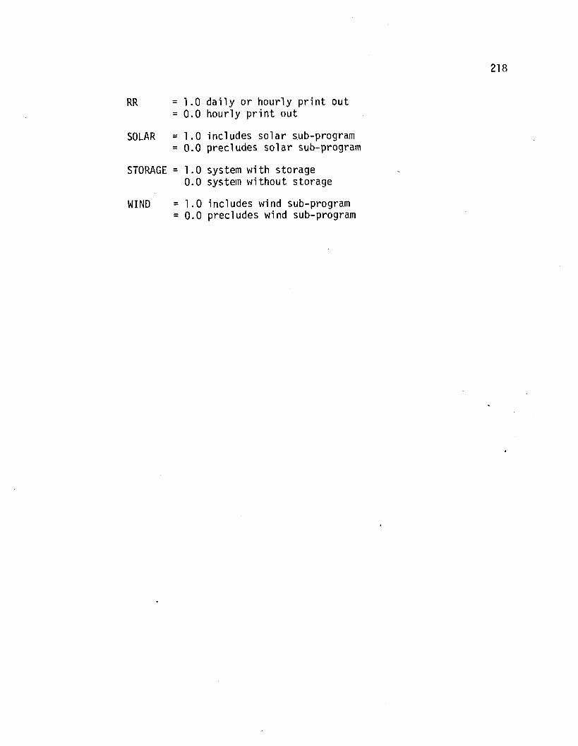
RR = 1.0 da i l y o r hourly p r in t out = 0.0 hourly p r in t out

SOLAR = 1 .0 includes so l a r sub-program = 0.0 precludes s o l a r sub-program

STORAGE = 1.0 system w i t h s torage 0.0 systern without storage

WIND = 1.0 includes wind sub-program = 0.0 precludes wind sub-program

MAIN PROGRAM FORTRAN VARIABLES -

degrees A1 : T i 1 t angle o f o r i g i n a l s o l a r da ta

A2 : L a t i t u d e degrees

A3 : C o l l e c t o r t i 1 t ang le - degrees

ABASDR : Area o f basement doors

ABASEF : Area o f basement f l o o r

ABW : Area o f basement w a l l s (separated i n t o sec t i ons depending on t ype o f i n s u l a t i o n , inc ludes : ABWW1, ABWN1, . . . e t c . )

ACEIL : Area o f c e i l i n g

ACOL : Area o f c o l l e c t o r

ADE : Area o f e a s t doors

ADN : Area o f n o r t h doors

ADS : Area o f south doors

ADW : Area o f west doors

AGRN D : F l o o r area

A3 : Thermal c a p a c i t y o f c o l l e c t o r

A1 : A2 i n rad ians

ALONG : Long i tude

rad ians

degrees

AWALLE : Area o f e a s t w a l l s

AWALLN : Area o f n o r t h w a l l s

AWALLS : ~ F e a o f sou th w a l l s

AWALLW : Area o f west w a l l s

AWE : Area o f eas t windows

AWN : Area o f n o r t h windows

AWS : Area o f south windows

AWN : Area o f west windows

AUX

AU XN S

: Percent a u x i l i a r y energy

: Percent a u x i l i a r y energy of systems w i t h o u t s torage

AUXT : Percent auxi 1 i a r y energy i n c l u d i n g h o t water auxi 1 i a r y

rad ians

2 B t u l f t h r

B A

C L

C M I N

CO F

: A1 i n rad ians

: Energy l o s s from absorber p l a t e

: Minimum f l u i d capac i t y r a t e

: Cor rec t i on c o e f f i c i e n t f o r wind speed a t tower h e i g h t

COH : Cor rec t i on c o e f f i c i e n t f o r wind speed a t house h e i g h t

COLCP

CON

C P

COT

D

D A

DEFNS

: S p e c i f i c heat o f c o l l e c t o r

: Conversion f a c t o r , knot t o mph

: S p e c i f i c heat o f a i r

: Cut o f temperature

: Blade diameter f t

rad ians

B t u l h r

: D e c l i n a t i o n angle

: A u x i l i a r y energy requ i red o f systems w i thou t s torage

: Auxi 1 i a r y energy , requ i red o f sys tems w i t h s torage

DEFS

DFSOL : D i f f used s o l a r r a d i a t i o n

DELTC : Change i n c o l l e c t o r temperature

DRSOLT : D i r e c t s o l a r r a d i a t i o n on a t i 1 t e d sur face

DRSOLV : D i r e c t s o l a r r a d i a t i o n on a v e r t i c a l sur face

E : Useful s o l a r energy c o l l e c t e d

EC : E m i s s i t i v i t y o f c o l l e c t o r p l a t e

EFF : E f f i c i e n c y o f c o l l e c t o r

EE

E G

ES

EW

GALLONS

GN

HA

HC

H T

HTR

HW

I

I I

NCC

N D

NDAY

NDW

NH R

NM

N TA

OVRFLS

OVRFNS

PCOL

P E

P R

P S

So la r energy through eas t windows

E m i s s i v i t y o f g lass

So la r energy through south windows

So la r energy through west windows

Volume o f water i n storage

Number o f g laz ings

Hour angle

Convective heat t r a n s f e r c o e f f i c i e n t

Tower h e i g h t

Height wind data measured a t

Convective heat t r a n s f e r c o e f f i c i e n t

Inc idence angle on a v e r t i c a l sur face

Inc idence angle on a t i l t e d sur face

Cloud cover

Number o f days i n t he month

Day o f t h e month

Wind d i r e c t i o n

Hour o f t he day

Month o f t h e year

Ambient temperature

Energy ove r f l ow o f t h e system

Energy ove r f l ow of systems w i thou t s torage

C o l l e c t o r s o l a r azimuth

East w a l l s o l a r azimuth

Prandt l number f o r a i r

South w a l l s o l a r azimuth

- -

B tu /h r

B tu /hr

gal 1 ons

rad ians

B t u l h r ftZ F

rad ians

r a d i ans

days

rad ians

rad ians

rad ians

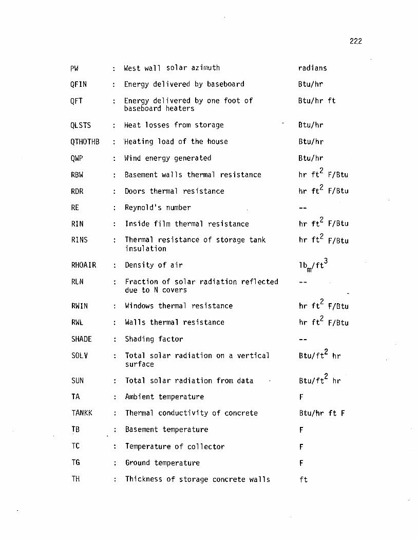
PW

QFI N

Q FT

West w a l l s o l a r azimuth rad ians

B t u l h r

B t u l h r f t

Energy d e l i v e r e d by baseboard

Energy d e l i v e r e d by one f o o t o f baseboard hea te rs

QLSTS

QTHOTHB

QWP

RBW

RDR

RE

R I N

R I NS

Heat losses f r om s to rage

'Heat ing l o a d o f t h e house

Wind energy generated B t u l h r

Basement w a l l s thermal r e s i s t a n c e

Doors thermal r e s i s t a n c e

Reynol d ' s number

I n s i d e f i l m thermal r e s i s t a n c e

Thermal r e s i s t a n c e o f s to rage t ank i n s u l a t i o n

RHOA :[ R

RL lV

Dens i t y o f a i r

F r a c t i o n o f s o l a r r a d i a t i o n r e f l e c t e d due t o N covers

RWIN

RW L

SHADE

SOLV

Windows thermal r e s i s t a n c e

Wal ls thermal r e s i s t a n c e

Shading f a c t o r

T o t a l s o l a r r a d i a t i o n on a v e r t i c a l su r f ace

To ta l s o l a r r a d i a t i o n f r om da ta

Ambient temperature F

B t u l h r f t F

F

F

F

f t

TANKK Thermal c o n d u c t i v i t y o f conc re te

Basement temperature

Temperature o f c o l l e c t o r

Ground temperature

Thickness o f s t o rage concre te w a l l s

THOUT : Water e x i t temperature f rom baseboard hea te rs

TIMECOR : C o r r e c t i o n f a c t o r f o r l o c a l t ime

TSMAX : Maximum s to rage temperature

TSS 1 : Storage t empera tu re "a t beg inn ing o f t h e hour

UBASEF : O v e r a l l hea t t r a n s f e r c o e f f i c i e n t o f basement f l oor

llBW2 : O v e r a l l hea t t r a n s f e r c o e f f i c i e n t o f basement w a l l s

UCEIL : O v e r a l l hea t t r a n s f e r c o e f f i c i e n t o f c e i l i n g

UGRND : O v e r a l l hea t t r a n s f e r c o e f f i c i e n t o f f l o o r

UTANK : O v e r a l l hea t t r a n s f e r c o e f f i c i e n t o f s to rage t ank w a l l s

VOLUIYB : Volume o f basement

VOLUMF : Volume o f f i r s t f l o o r

V S C A I R : V i s c o s i t y o f a i r

W L : House l e n g t h

W P : Wind power generated

WW : House w i d t h

Y : Absorbed s o l a r r a d i a t i o n

Y FIN : Length o f baseboard hea te rs

DOMESTIC.HOT WATER SUBROUTINE FORTRAN VARIABLES

DEFHW : A u x i l i a r y energy r e q u i r e d f o r D.H.W. Heat ing

DMASS : Mass o f wa te r i n s to rage

1 b f / f t 2 sec

f t

HW : D.H.W. requirements

QDHW : Energy d e l i v e r e d by t h e system f o r D.H.N. hea t i ng

QHW : Energy needed f o r D. H.W. hea t i ng

ROWTR : Dens i ty o f water

TCW : Cold water temperature

TDS2 : Temperature o f s to rage be fo re D.H.W. de l i very

TDS3 : Temperature o f s torage a f t e r D.H.W. d e l i very

THWH : Upper l i m i t D.H.W. temperature

THWL : Lower l i m i t D.H.W. temperature

TIiWR : Temperature o f D.H.W. r e q u i r e d

ECONOMIC FORTRAN VARIABLES

ACCONV : Annual f u e l and convent iona l system c o s t

ACONV : Annual convent iona l system c o s t

ACOST : Annual c o s t o f s o l a r and wind systems i n c l u d i n g a u x i l i a r y

AC S : Annual c o s t o f s o l a r and/or wind system

BCONl : I n i t i a l c o s t o f t he blades

BCON2 : Present c o s t o f blades

BCON3 : I n i t i a l c o s t o f t h e blades

BCON4 : Future c o s t o f t he blades

CBS : Present c o s t o f s t a t i o n a r y p a r t o f t h e w indmi l l

CBS2 : Future c o s t o f s t a t i o n a r y p a r t o f t he w i ndmi 11

CCOL : Present c o s t o f t h e c o l l e c t o r

ga l 1 ons/hr

B tu /h r

I b,,,/gal l o n

F

CCOL2

CDEL

CDUCT

C FAV E

CFUEL

CFUELl

CFLlR

CGEN

CGEN2

CONV

CSOL

CST

CST2

CSTOR

CTWR

CTW R2

CWIN

I

N

R I

Fu tu re c o s t o f t h e c o l l e c t o r

Cost o f hea t d e l i v e r y system

Cost o f a i r d u c t

Average f u e l c o s t

Annual f u e l c o s t pe r Kwh d e l i v e r e d

I n i t i a l c o s t o f f u e l

Furance c o s t

Present genera to r c o s t

Fu tu re gene ra to r c o s t

Convent ional system c o s t

Cost o f s o l a r system components

Present c o s t o f s to rage

Fu tu re c o s t o f s t o rage

Cost o f s t o rage

Tower p resen t c o s t

Tower f u t u r e c o s t

Cost of wind system components

Percent i nte res t r a t e

A m o r t i z a t i o n p e r i o d

I n f l a t i o n r a t e o f f u e l c o s t ( pe rcen t )

$ / f t 2

6

$

$1 Kwh

$1 Kwh

$1 Kwh

$

$

$

$

$

$ /ga l 1 on

$/ga l 1 on

$

$ / f t

$1 ft

8 - -

years

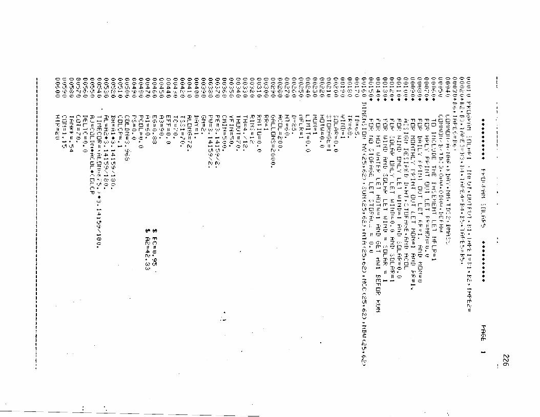
3 5, LC ro c-

b3 I II 5. C

4 CC'

C

P C

8-n *.is

C

qlia '2

C ,= i-Q I,.' a=,

+ x

I1 L

I-.

fin

= . .

',.I ,= ,z

m .m

I 1 I-.

-= .= I-. p. C.

t? CI

J A

C A

1 . 1 -

CI

E A

T -:I

rlib !LC

b?.

rbct . .

I,,

C I .. n: 1-n

37. rll .d

7 A

-a

2

rc cr 17 r t~ lL.'

" - * 1. ' 1:.

.- r~:, iJ1

B. rt:* 'U

" 7 A

'3 :-- - .h

rtr I-P

q7: rn.1 b

c. -3 ,=. c, C I-.

.b i.~j

.=, .= 4 4

-rt 7, C G 7-1 T

I z 0 - 4 I e -

.- I' $ I A n? r T :n . .

J..'l

!- 0 m r -.r IT! r z r-

5 P? z. + I! e .:

CI

5 2 t?

I I 1; 1 p. ;;:, -I c r

1 F c n C

I I m m - n

% . - 1-

I

11 1.1 P:. 1 id ([ IF= i . tI:_:T+-.t.:,<,*LlLUl>1 0 I... : : (14$*~1 +q.;'L;?:!., i.. 21-::>7+,t556+L1~u1--1 11 I ' . ::LI-?:~: (l<Iy.;'_'o+ bHTF'+il. 1 5 i > 0 u& ::(I I: ~H=I. I . :i;,71 11 I:I c, 4 r! I>I:E I L = ~ I . I:I~ '3; F I J ~ F ~ . { D = ~ . 111 1 5 2 l-lIje.5 0 l!lL-=4:3. 7 % IJl,!=.~z. (17 11 I.I&~, 1.1 <il: 1 L=I!II~I+I~IL 0[157 1.1 HF:A: ~ F = F ~ I ~ L I ~ I I = ~ ~ I : - E I L (I 111 6, :i: (I til,!l{= 7 2 . 2; Hll!i:=48. (! 0 c, '3 I:I tll,lL= t-4. 2 $ f;Rl,~I=%.l. [I 11 7 0 111 t l~ l l i= ld. I! !it HU2=21. (1 (I 111 7 1 I! f f I ~ E = > l . S HUIII=Z~. (I I:I ZC 11 ~ l ~ l f f ~ - ~ ~ = l , I ~ , ~ * : ~ . ::..fii:lE-~IlE (I 111 7 :; 1.1 LHFtLlE=il. 1 1 1 0 7 4 111 HE=filnlE* i 1. - :HALIE) [I [175 I:I Fil~l=Fil~~l!l* 1: 1 . - 1 HtiIlE.? [I I:I 7 6, f j H ~ . = ~ l ~ ! i + i 1 . -iHAr~E.:f i (I 0 7 7 l:l 1 71 l-y..:, .: ;: = I? F, 1- L [;pi .,I, * ::: . '1: 3 11 I~I 7 :E: 0 TH},;',,.'D~-.; = 1 r.10; -I ~. . . . g? 4 0 079 l:l -. ILIE>=T!~\:'-;UL ;++. ::.34 [I 111 !f: 6 I) f i rAp{t:.._:=~y.. .: 1 LIE;*:: I LIE> rg 0::: 1 111 ~ l # l ~ L L l ~ l = l ! ~ l ~ l * : ~ : . -~l!l l! l-~ll l.~l

(1 :- ,-I *L . IJHk- 1 '& t.iIlA','=l I~I E; ,!: I:I H I J ~ ~ L L : ~ =ld~*:::. -Hlll,z -HI!.?

r~ [I ::: 4 I:I ~ I , I ~ L L ~ ~ = I , ! ~ - + ~ . -~l, l r i -nl lr{ (I 111:;; !:B CI ~l:i!ll,tl 1 =i(t.I.o!t l- l , i I~:* 1 . 0 1:1:36 (I AE:l,l ;. 1 = l ! l ~ * 1 . 0 I);!:? 1.l fiE!loll{ 1 =lslL+ 1 . ,j 91, .:, - a-o ,-. lj 11 fi 1 F: = 1.1 . 111 (I (I [I 1 2 0 (I&? [I ~ I , I I - = ~ ~ ? . 6 F:kl!!l=41.4 n u.3 cl I:I PF'= . 'a I I-

(I 0.3 1 1:l T::PtA::<,== u. 0 11 *? .=: 111 k:~!!IPi=lc~. 1 I 0 lj.3.z: 0 F I I F . : = ~ ~ . 24 lj (I 4 I~I 1 1 3 ~ 5 111. f LP=0 .24 (I [I+? I:\ IJEh.::EF= 1 . ../ 16.. [I [Is> 6, [I UbI.nlz= 1 . ...- 17. 2::: b

(I 1:l'i; 0 '\:OLl-ll.tk:= 1 I: I:q 111. 'fi './OLI-IMF= 1 2 5 00. (I 0'3:s [I ~F:l,~l!~::=I,:i,j*;. 5-5. D*5. 5 lj O.39 I) fiE;l!l>= 8 I ~ I I ~ I + ~ . * l . n l ~ : ) *:*, 5 (I 1 0 0 (I fiE,IJ 1 = ~:.1~llo1+~. *I,.IL,I +:3. 0 1 111 O p 1 14 = 111 . 6. :k; (11 0 2 0 UTHNk= 1 . .I cF: I rl+F.: I1.i:i:+TH..s.TANk.K) (I 1 ~ 1 3 11 Pi= 1 01 0 4 0 I:. C: = 6 1 0 1 050 rib\= 1 01 ( i e . ~ 14D='313 $' kmY= 1 (1 1 0 7 11 At:Ai.LZ1P=5<, . [I 1 [1:5: (I 1 F i..>TlJF'HI_.E. El:!. (I. I:I'.I lT,ALLOI.i'::= ij. 0 (I 1 0 9 111 I F : L l l 1 T . ! . l . : 'r 'FIN=O [I 1 1 [I 1:l IF~~;-ULAF'.EI;'.I:I.I:I? AI:UL=I:I.(I (I1110 F'EIPIT 16.'?5. D. HT w r lF LF'. AI:.~~L 9 I3hLL.Dt-fS ;: "IF I N (I 1 1 2 [I 1 4 T 1 i.'30!l1IINDr U L A P ~ H ~ T I ~ l r >:lLIF'AI>EyF:fiTIO Cl11:;[1 12[1 ~ : ~ p ~ T I t i l - l ~ 0 1 1 4 0 E . . 1 C ! i . Z l - l P i i 1 1. .JJ:? .lll:l:.rl I r.-lJ,~ r P{'r:(l I r JJ.? ,NTRc.I I r J . l i r (11 lt;O+l.~Lll~lr 11. -1-1, !, 1 1 ~ 1 . 2 4 ) ..i.-l=I:~lrC..k) 0 1 ] ii, 0 I F l . t i r l . ~ l ~ ~ . 1,: FPIMT 1c.21 ~1 1;[1 .::?[I I - U ~ ~ T 1 ~{I-IE (J 1 1 5: [I .;: 2 2 I,! T U T 11 = <I . 111 01 1 5 0 I.,! F II= I:I . I! (I 1 2 i~ 11 IJl,!p11= i~. [I

Cl 12 1 I) :: 7 111 '-,.'=t!,.! * 1 {Hp . r1 ['ltqa.(' 1

11 1 3 2 i l C L . i . d L = ~.l-lI{ t ! { t j b , , + ri[1t3'~':1 (I 1 2 2 111 1: 1: =ric:1;. 1. I-it{k, , riL4FI.y' b

(11 24lJ 1 h=I*TH <l1tlP* l{Ttfi'f> (I 1 ;:3 I) l!i[l~Vi[lI~~ 9. l.itjK. r4r16i.r') 01.26O I,I't.'=';?+I: IJIJoC LjF [I 1 2 1 (I ~ ' :?= 'v '+ I: u r i c ~ : . ~ ~ 0 1,331) IFi.ldII.4L1.tl:l. I.! IXI I L ~ ;,4r1 (I 1 29 111 I F i:.IuLFfF . EC!. 1 . .:I 13fi TO 706- 01 ~[II.I ;--.41j CUIJl-Jril>t-. [I 1 '5.1 (1 ~ F i : r l . ~ l ~ ! . ~ l : l . : ~ I>O TU caSO lj 1 ,j: F: [I IFI;D.EI:?.LS.~ 13Cj TO f2E.I:l.

0 1::.':1;0 IF('I.EI:!.:::~.~ I:;IJ 1 0 C,:~[I [I 1 :::4 0 IFt.Il.E!.1. .I;=. 5: I ~ C I[] ;,73 r .1135~ IFI:II.EI:I.:::~.~ 150 TO g9 i1 (I 1 2: 111 IF<D.EI:?.~I).., 130 TO 7lJ0 (ll'>il:l C.5i.l I F i.I,I1,:.L,E. ~ : . ~ . ~ ~ : . l , ~ ' - ; . l ~ ~ . . ~ ~ , . 1: )ca: ,4 ,~.~,~ U1::::311 g.55 lo~P=-.41: i~+. 1:~4.:;*1,1:,!-. 1);:~::4:3*1~1~:.:*1,1'~~+. I~I)~~.S*I.,.P\:++~.-. OU~I~~~:::*I~I:;++~. Cll>*gij i:.!54 I F c:ltl'~,'. LE. 2:. 5,;t l!J!='=l:l. [I

0 14 0 f! I F l:l~i'-;. t>E. .36. 1 .:I I , I ~ = ~ Y . 0141 i l T O ~;.'I:I

(11421') ~ C , O I F ~ I J V . L - E . ~ . ~ ~ . D R . I ~ I - - ~ ' . I ; F . . : ~ ~ . l:rbt,4.1;<,~ 014:1;1~ c.t.2 !,li.=-:?;2;.::+. .r;Z*l,l'.:'-. I:I::JT'*(J~,'+I,I'.,'+. rj?1~3~+I,lt.;*+:::. -. O ~ I I ~ I : ~ ~ ~ ~ + I J V + * $ . 0144(:1 <.c.4 1Fi.l,I',:.LE.-1.4~:? l,lf-'=O. ij [I 1 4 5 1.1 IF<l!)'\!.l3E.~;l, 1.1, l!lF'=25. @l .?C. [ I 5 0 1.0 ,37ij (I1470 <,['; I F ,.IoIp~:'.LE. 5 . 46. GF'. hl'v', GE. E'b. l>Er7h. 6 ' 4 (11.?:31:1 674 blF '=- l .:;:7.)+. 521*lJ::'-. I~IL;*l~l'-~*I!.l'\?+. ~ l l ~ l ~ : ~ * l ~ l ' v ' * + : ~ . -. 506°3E-4*~dV+*4. 01450 e.76 I F t.ItI'v'. L E . 3 . 46) l,!F'= [I. [I

0150i1 IF <I,I~Y~.I~E.Z~,. 1) I J I F ' = ~ ~ . I:!

0 15 1 il 130 T O ,370 I I I F n.:l!I1*.!. LE . L-;. [I.OF'. l , l ' ~ ! . I ~ E . ~ 7 . 5 : > 6 ~ : 4 . 6 : ~ : ~ (115:::1) : II!F'=-~. 5t+s++.4s35~+l.d't;-. 051:3~,+lrl~,t*1!~',:+. i11:1:34+1&'+*'3. -, Q~IO~:::.~.~+IAV++~. 015a4Ci &:34 I F a.l!l'~'. 1-E.5,. C1.i ldF=[l. [I 01550 IF CIJC?. 1I.E. 27.5.) I!I~=z,. o 0 15~.[1 130 1- 0 9 7 I:! i11s70 15'313 I F ~ : . I ! I ' - ~ . L E . ~ , ~ ; ~ . U ~ , I ~ I ' ~ . I ~ E . ~ ~ ~ . $ ~ E . ~ ~ , ~ ~ , ~ ~ - )

(11580 r.'+i' r,tF'=-c,. 'l;,?g+l. :3El+~'-;-. ~~+?:-!+I,I?;+I,I'.,;+. i~~ti;:e.+~,,lr)++:>. -. 0001 17+l$lum*+4. 01530 t.44 I F i:I~l '~~.LE.~..5f; ' , InJF'=l:l. I) @ 1 c. 0 lj I F <(I!'$. 6E. 24.5: l!IF'=55. (1161 o GU r0 ,970 olheo 7 0 0 IF I:.~!':!.LE. ;'. 7 5 . ~ ~ : . ~ 1 ~ . ; . 5 ~ . 2 ~ . 7 ) 7 1 1 4 ~ 7 1 3 2 C116'3O 7 0 2 IJF '=-~ 2 . 1 i j71 + 3. 1;7+l,la:!-. ,5::f:7*Wsi**2. +. 1j13~96,*M!;++:3. -. ~ 0 0 1 : ~ ~ + l ~ ! i t + + 4 . ( I lc040 7u-4 I F I..IJ'.,'.LE. 7. 73:) I!I~=[I. 111

(11e.5O I F 'u'~;. ISE. 22. 7:j LIp=EF;. 0 I) 1 <,h cl i.U TO -37r.l 01c.70 -370 I~I~~I=I,IF'LI+I,I~ O~~:::I:I 7516 CUI-il II-~I-IE 0 1 ij 9 111 I~!!,IF=IIIP* 34 1 .3. (I1 70i.I IF(.riHF..GT'. t..HPiD.liHF'.LT. 19) 940r4(10 01710 51:ll.l EE=EW=EZ.=IJ. I:I (11720 TI:.= Te u173[l 152 1u (11741:l ir41:l IFI:.TI::.LT. TAr Tl:=TA (I 1 7 5 [I HI.'=I-IHF' 01 7615 Hk=HF+T I PlEC OF' 017'70 De=Z:j. :jt$.1'..,, 18111. + 3 . 141544.5 IN i2 , +3. 14153,,':265.+ (DH'i+lh3.:j> 0 1 7:3 1) I++ I : .HF: -~~ . ) e.3. 14lrgy.....1?. (1 1 79 15 .-I I!! 1.1 [I = 1 Q 1 2: 1:) 1 j I F rHn.E1;1. U. 11, 1:,0 TO ~ $ L I

11 1 :3 1 I:I IF~.HH.I~~.I.I.I:I:~ 150 1 0 '372 0 1 :3 ;: [I F'=pE lj 1 5: .I; 11 130 TO >~[ I IJ

0194 15 '3~,1) ~ ~ = r i ~ + y LI 1 :;: :, (1 k.t,t=~. (I 1$:6U 130 TO ,+~I:I

[I 1 3 7 1.1 *:4~z -lt,lrj[l=z (I 1i::S 0 F'=F~II [I 1 !S.+ 1:) 5 0 10 >1:11'?1:1 illa~I:lij 5 7 5 El!i=~l!l+'.( (1141 0 (1

(I 1 9 2 1:) 11. [J 1 0 '3 '3 111 (1143D id:::^:^ EE=EI,I=rJ. 111 (11441:1 4 ~ 1 .-II,U~LI=~ (I 1 4 5 r? F'=VC CIL ljl'3e.O ~ 1 ~ l I j l : l CD.l.1 1= t:<I!.i 1.UL.I +1::0.5 ':.E:H'> -1-.J:s: ~.:fiL:, +Z:I I I i'L:A'*1:.05 i :P i i +:.I.INi:Dfi>

- (11470++ i:lI.fiz: 0:HL) *IIDI. 1: Eri) +..I. I ( J I fiL.18 +..:II.{ i.t:H::t *[:DL: t..p:> :I +1I.u5 i.Dfi> +1_'05 iH&> (1 1'<3:::[1++5: 11.1 o::k;* 1 :. 1 r.4 o:F.:l *1:.n,:: 0: 1,tq:* +.i. ] p i *:wfi.:1 (I 1 -3 t3 111 rI.Ui.l=:_ ]pi <.P? +l:U':: !.IIH:I * < I N *..HHj +':.lt* (.AL'r +C:O:z CP:! *11:0:3 inn'> *C.O:: !.HH:i ljzr?(t(~+-II:n:- (HL::* + I : ~ - Z i.F':* *<If{ I:.L~~.:I [I 2 111 1 [I ti I 1 =UC:(-JL. (,I; 0.5 I 1 ? (1 -2 (1:. (1

L - L . I F # ' . H I 1.15T. 1.5i1;1:3,i A I 1 = 1 . 5 7 0 7 02 0 3 o 1 = ~i I:: 0 :, ,:: I:: u ,> 1 ,:, (I 2 0 .? 111 I F I .RI . 151. 1. 5713E::l h I = l . 5707 0 2 05 I'J . j ]p{f i :=z I P { i , f i I > .."1 ,52 112 i j f . I) p = fi 2: 1 1.4 ,., ..; 1 1.4 $ ;) [I? 07 [I 6 : ~ s . 5+ r i ::I!( I QI-i;..:! *: ~ r i I'.~I-I.:) .:a ./ <:.<1pi i.fi~+~;.:) SIP^ <HI+R:, .r + <TH~{~.HI-F:S (I~I:I$:I:I++TH:J ( .BI-P) :I .. 1.Tyri ~ , . r i I +p , + T h t i I:AI+F:.> :r :, (121jgD r-:LP{= 1 . - < e.: 1 . - ~ L , J .,, 1. 1 . + 1.2. +15ri- 1 . .I + k L l (12 1 [I [I IFi;15ri.E1;?. 1 . j PLl=C1.16 (121 1 0 IF ,511. EQ. > . > F'D=I.I. 24 0 2 1 2 0 1 F i.Gpi . 111 . 3 . :! F: p= I:' . 2 '3 (12 1 3 i ~ I F ~ . A ~ . L T . .5 ;::;;1...1 HE:-=lj. 96 OE 1 4 I:I IF i.61. I ~ E . . 52:::6. ~ r i D . fiI. LT. . g,*3:3:) h)'i.:=O. g5 (12 1 5 (1 IFc.HI.15E. .&,'+:::.firjp.HI.LT. .:_':7P<,., eB:::=rJ;3:3 (12 I 6 I:I IF ~ A I . ITE. . : j 7 2 ~ . ~ P { D . AI. L T . 1. 13472:) fi~:'5=1:'.31 (1>170 IF i . u ~ . I ~ E . 1. [1472. fit-ID. 01. LT . 1 .;el 7:) ~1:'5=~1:3:2 - L

l j Z 1 5 0 IF (el. GE. 1 .2217 . fib(^. fi1. L T . 1. 396:3:? ~ b : 5 = 0 . (12 [I I . - I . I : FIE:;=I:I.~.~. (122 (I (I 5 I p l f i f j = . i I p i (AL.:, +:<. I ri I: rlfi.:~ +c.n.s ~.HL j +I::US i.Ufi) +C.OS iHR) 0 2 2 1 111 A i ~ = f i j I t i (5. I pii~H::~ 0 .;. .:..= LLL - DF:?uL= [I. T:S+<. 1 . .s+Hfi+c,. 17+11.C il :. .-..-;; I'i

LC- . I F i:DF.I.OL. LT. [I. [I, DF.ZOL=O. (I 0224 [I [I~T."S DL T=CUL-LIF':OL (1225 (I IFiLlF.:.~.ULT.LT.[ i . (1.) s (110 .2015 (12&.13 201[1 [IF:_:DLT=O. 111 (122 7 (I DFS.OL=:.I.:OL rJZ&'$:l:l 2 [I 1 5 C.ntiT I NI-IE 0 .Z* 3 -3 il LL . . DF:;:.OL'.,?=DF'I ~ L T + I ; D ~ I ...'C'OS I 1

02.3(l0 50L1$=DF~CL~, /+DF" UL 0 2 3 1 0 I ~-[IR:~:OL.'.,'+ I _ c. 1 . - F ~ p i r *AL::<.+[IFTOL+ (,I. -F'D) • (0. 30) 0232 I:I 1 F i, 'T' . T . [I . 111 > '.( = [I . 1.1 023 :: 13 I F ( . - I I ~ ~ ~ ~ L I . E I ~ ~ . 1.1 130 r o ggn (12340 , I F r .-lblr.iD. EC!. 2:) 5 0 TO ,375 (12'55 I) I F (.Jl!l~i[l. El>. ::,I ES=Y*HS U , 3 c a 0 EIJI-{~IIJI=EE+E I.+EIJ 02'37 0 I F (SULWP. LI;~. I:I. <I> GO TO 2205 @E.SrS [I [:=(I. 1'3-111. I.ICII'~:~:~*H.~ 02 39 0 H13=1. +!:I. .jO4*n1,r (1,3 u 111 I F 1HV.Lt . 1 i 1 . j F=l:,.76*11:1.**(-. (1325*H'$>

C. Jz .=, rl:, r,

or-, . - C I...',

m '2 ,:...', II

1 3 ,

t-.

2 1.'

C n ,>:I , >:,

a& * '3 ,-* .= TI-I rt:f . . t-s-9 I-,:# re c ,=a <a:,

Y Y

n T .?.. Y'+ ,,..'* 4,..'!

I:.'.' I,..'" c. C . . 831 CI I . .

C -.,j r,:l ,=a . . . . . . . . - - Gi r1:i

G:I r1.*

--I .=. f l a

ru rtj i.,j i.,) 17,

a=

1-11

C 92 '.I.' C

,=,

- ,.. , I..'! - .- I1 rn

-4 I C1 c .: 0 C D - ,. ,

a','! - -

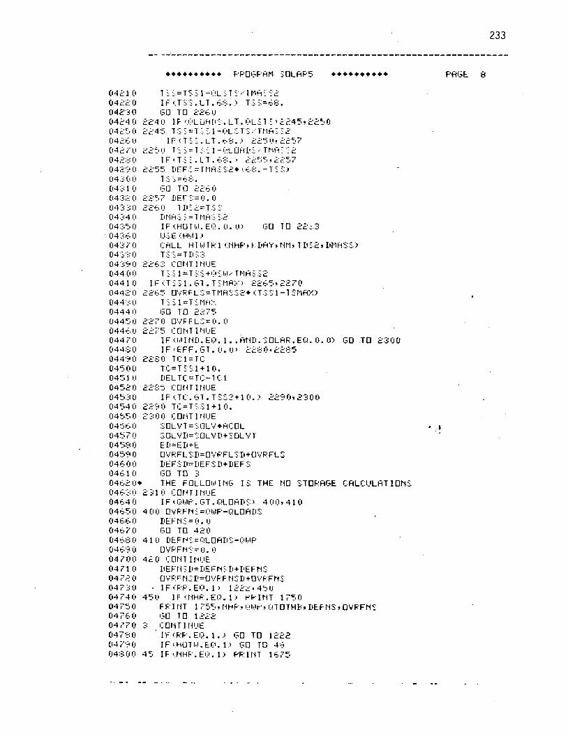
(1421 0 T..:,..:,=TT.;; - - - 1 -I;,L;,T 1,.1 ~2 oil>= 0 I F <.TI'<:. LT. ; . :3 . ) T.I,;:=<.g. (142.3 I.? I ~ U 1.0 22E. l~ (1424 0 2241:1 1F ~.I:ILU~~II.::. LT. I::IL<T~ 122459 $250 (14~~,1:1 2 2 4 5 T ~ ~ , ~ , = T ; . ~ , 1 - 1 ; ! L , ~ , ~ : ~ ~ . . ' ~ ~ ~ f i ~ 7 _ L 2

(14>i31.1 IF i T::. 1 . LT. &:3. ,) 225 111. >;:,7 ( 4 z . 7 ; 1.1 ~ ' y ,- - T ;r 1 -C,L UF~LI,: .. T p,fi.~.'z 2 ,..i LL- . _ > . - 04,;_'::: 0 I F i: TZ..:. L . c.:$:. :, ztrjf,, >;:57 (142'30 ,5+25:, I ~EF : :=Tp l f i < : z :~ *~ .~ . : _ : . -~~ : :~ . r [I 4 .1: (I (1 Tz <=G:E:. (14::: 1 0 130 T O ~ ~ - . 1 ]

(14 32 (1 225,7 fit-$'::= I), 0 Cl 6 1 :>:2 1) 2 2 6 cl 1. D ,7 2 = T 5 3 (I 4.3 4 (I Dplfi:i.>:=T p1fi.L. '5.2 (14:>'_, 0 I F I:.HU'TI.J. EB. 1;l. I?., 130 TO 22.: 3 (l4:36 0 IJ:T:E '.HI!! 1 ., (14 3 7 (1 I::~LL HTI!!TI;:l !:I.{HF',~..DH'~',~{M,TD'ZZ~DMFISS:) lj4:3z 111 T 5 - ': - - T 11 .? ;. .:. .-.

(1 4 .> 9 0 ,, .:' '2 6 -..-. '7 COIiT I PiI-IE 044 0 (1 T;:: 1 =TSS+Q'<.IJ,; Tpl~:s.72 (I44 1 0 I F r.T::Ll. 131 . T.:I.lA:,:> =zE,5r 227[ l (I442 2 2 6 5 041,!R'Lz=Tp1A:i.5L>* I:,T:<:.~ 1 -TSMBX) 044':: 111 ~'7;';; -. .& 1 =T: plfi:-, 0444 111 130 1- fl .=, .:, - c

L C , 1

044!51j 2 2 7 0 IJ':?FFL.~=I:I. 111 044E.O 2 2 7 5 11nI.iT IPiI-IE (144 ;' [I I F i.lrlII-ID. 150. 1. . HHD. SOLHF;:. EB. U. 0) GD TO 2:30U (I 4 4 5 I:I I F I:.EFF. GT. (I. i:~.) 2;:'iO. =2$5 0 4 4 9 2 c,-,l:~ .-. .=, TC~=TI;

045 111 0 Tl;=T:::<:l+l 0 . (1451 I:! DELTC:= TI::-^ 11.1 0 4 5 2 0 22E:S CUIi T 1 I.{l-IE 045:s (I I F < T i : , I ~ T . T . ~ ~ . : ~ + 1 0 , : > zz90rz '>( I0 (14540 ze,31:1 T F : = T S . S ~ + ~ D . (1455 0 2':: (1 I:I C.OIiT 1 NIJE tj45i3 111 SOLVT= iflL1\!*Hl::OL 0457 0 ~ a i ' v ' D = ' ~ . ( J ~ V ~ ~ + ~ ~ [jL'.,'T (1458 [I ELl=ED+E 0 4 5 9 0 U'h:'F:FLz:D=O',:I;'FL:I:r~+u'I:'pFLS (I 4 e. [I [I DEF$D=IIEFSU+DEF~ I]4E0 1 0 6 0 TU 3 04i iEi l+ THE FULLOI!! I PIG I:S THE NO S:TOF.:FlGE CfiLC:I_ILHT IONS (14c.5l:l 2.31 111 Cnl{TINI-IE 0464 0 IFI.ISI!IP.GT.~~!LO~~DX:> 401:1,41(l (14e,5 o 4 o (I @'V'F;:Fld 5 =I;II,I.I~-I;!LOAII:;: (14iffj. 0 DEFI.i:S=li. I:I 0 4 6 7 0 5 0 TO 4 2 0 04<.:3[1 4 1 [I DEFI.{:-.=BLOfiD~:-1.:!l,Ip (145'3 (1 u'v'FFNS=l:l. I)

0471:11:1 4 2 0 IIOI.iTIf4IJE (1471 0 LIEFI.4 5:Ll=IlEFN:_.D+[lEF Nz: (I 4 7 ,? 111 U',:RcTt{.;:I1=fJ!:'F:F I~+o;:eFp{z: [1473(1 . IFI:F:F.El;:l. 1 > 1 E i z . 4 y i j (14741:l 45111 IFIP~HIT.: .EI~.~.:~ +PINT 1 7 5 0 (I4 75 11 F K I riT 1 7559 1-1tiF'r BC!F'r I:?TO'THEr DEFPiS, OVPFNC' (16+76 0 150 To 1."2z 04.270 3 l : . u t i r~~ i l -~~ (14750 1FiL:P. Ela. 1.) 130 TO 1 2 9 2 (14 7'3 0 I F ~.kiuTlJ. kU. 1.1 150 To 4;s 04801:l 4 5 I F I.NHF'. El>. 1.) PF: 1I.iT 1 6 7 5

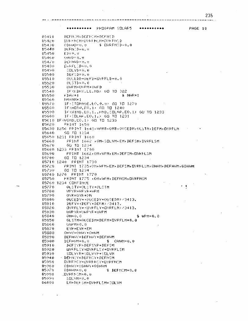
+**++*+*** ppO13F;'fitI EOLfiFY ++****c*e+ F' ill-<E 1 [I

i t 5, 4 1 o IIEFII :~;=r~t_f--rr: i ' l+r~EFr i f rl 0 t, .% 2 111 !I'.,'F Fti!Pl-LI'::I- F h LFl+i)':.'k FPi- LI (154 2: (I I:IIII{IVIII=-I.I. I:I 'f. L] I,.' F: F 11 I I -I I:I . I:I 05-1 4 n LIL-:FI~ : r ~ = 1.1. 1-1

(I 7 -1 :al:~ [< 1 I = i~ . 1.1 (I ':a 4 c, I! l ~ l ~ ~ l ~ ~ ~ l = l ~ l ~ IJ

05370 J ~ ~ f ~ l j l , l J ~ : = I!. 1.1

(I 5 4 :I: 1.1 u as; F F L 11 = 1.1 . I:I (15.1'9 0 .I. u L by1 LI = . [I [1'>3 [I iJ 11 E F i. 11 = I:I . I:I (15% 1 111 1:!1_1: [ILI=~I~FLI=L>YF'FLII= ?I. 0 (155,' 111 lYlL'>lLl- 1.1. I:l (155':: 0 I-IIvI P PI= 1-1 1 . i F' PI+ 1) la! F' LI 0 s '_, 4 I:I IF~~.IIH'~'.LE.~{LI.! 130 -ro ?=,:- .LL

.fI"55 0 Ll fi '.,' = 1 9 t4tiF.:= 1 (I :, 5, c. [I riPl=PiPl+ 1 (IS5 7 I:) IFI.Z.TDF'~~I:~E.E.~I. 111. [I.! 150 7 0 1Z;'lj (I 3':, ::: [I IF 1 . ~ 0 T I,[. EIJI. 1 I IGU T 0 1 2 4 CI

[I a? CI I F i<I!!II.iLI. EIII. 1. .HI-{LI.:IOLAF'. EQ. I.! 60 7 0 12:>:3 lj50S (I 0 IF~.:OLHF..EI:!.~.::I 13n 10 1z. I : l (Iy5,l (I I F ICIIIJV{I!. El:!. 1.1, To 1.LL'-"- ,- .= ;' 055.2 0 F'PIr I l ' 1<,51:1 (156-:!:1:1 12:'5c. FF' I r iT l < - . ~ : ~ ~ I ~ I F ' P 1 E ~ ~ I ~ ! ~ l ~ ~ ~ ! ~ l ~ I ~ E ~ I ~ ~ I ~ J 1 - ~ ~ 1 . ~ ~ ~ E F M ~ ~ S , ! ~ F L ~ ~ (1564 (I 130 TO 12 I :4 (I'.;e.!j,[l 12'::l FRIPiT ~<.C.I:I (I 5 5, c. 111 F'F'lPiT 1c.c.Z ? l l l p l ? ::.OL?'Pl? EPl- UEF'..Pl? U'V'RFLSFl 0 5 6 7 i l 130 TU l,:::.lr (15- .I 2 1 1 .=, .:; -< I ,.-- p ~ ' 1 1 - 4 ~ 171)1:1 (1569 0 F'PI 1iT 1 caEn2. <!PI! I!IF'Pl! DEF5.N. O'v'K'LzM (157 0 0 130 TO 12:34 0 5 7 1 0 1241:l FF ' INT 17.20 (It;7;:[1 F'F' I t41 17.35- IC't.lr IIIFPI? EM? DEF.Stls D1\*EFL>Pl? ~;!hl~lPlr 11EFHhll.13 QIIH~IM 0' -.-<

- t i - 130 1.0 12.34 (15740 1 2 7 0 F ' f ? I b i l 17TI:l 05750 F'F.'IPiT 1 7 7 5 - ~IlPlr ldF.Plr DEFfi:.T.l'l, D'~'kFri5.N 0576. :',0 12:34 C T 1 PILIE (I577 [I QL 2 T'~'=I;IL'I: Ta<+1IlL:S TM * b

0578 0 l.,lp'<F:=I!Ip'.{F+I,1pp1 (1579 0 QYF:=l:-!'y'p+[~p] CIS@ 0 [I I;! I&. E 1 1 ' ~ ' = I:. I;I U.I. E 11 'r' +I:! 1-1 ': E 11 P I ? . / : I : 4 1 :s . (1581 [I DEF'r'= cIlEF'f+LlEF p1:1 ,->.241 '3. 0 5 5 2 0 i]':?PFL.'y'= 8 U'::FFL'<+O'~:'F:FL~.~,:I /:34 13. (15E::s [I I-IIJF'fF=I-ll~i~\ F'+I_II!IF'M fjsz:.? 0 I;! PI = [I . 111 % MF'Pl=(I. 11 0 5 9 5 0 I~!L'~TM=I~.!I-I:E:E~~M=DEFM=D'~!F'FLP~=I~. 0 (I'i::e. 0 l-lln~F'tl= I]. (.I

(15:37 0 E'u'F.:=E'IF:+EP~ (I :;:s 8 (I I:IHI~I'~=I;IHI~I'~(+I~IHI!I~~ 055:p lj LIEF HI,I '~'=LIEF~I!~'~'+DEF~IIIM (I 5 9 I:I 0 LIEFH~IP~= 0. I:I 'f; OHl,,lPl=~j. [I O!f,"l 0 ~ I E F .T')'P=IlEF'?'fP+DEFf b l 05'32 (I U'\CFFL ~.'<=uC'~FL'~'r '+T_l'.{PFL~ 0593 0 ";.OL?~'y'F'=<,UL',:')'~+'~ UL'V'M (15'3.?(l . IIEF!~'I '~'=~IE}Y~{:: '~'+DEFI.~'. :~I (I 5 4 5 111 D',jF'F;{'? '.(=L]?,.'F'FIf <'f+fi'.,.'PFr{,I M (I .:, '' E, [I l~~ I l~ l~ l ' <=~ : !L~H l~ l ' y +l;lI~H!~!pl (15 1 4 7 fj I;ILIHI,IP~= 111. 111 '?; DEFriIPI=O. U fj'_,9$1:1 .U:..'pFN:tq=0.u (I :, .3 CI 5 u L- t,! p1 = 1:1 . 111 (I 6 f> 1 1 111 EP~=[IEF i p l r - ~ ' r . ' ~ ~ ~ c n = _"OLVM

1 I:I 10 1.1 I) s 1 - 1 k : ~ ~ ~ l - t ~ i ti^ HIIJIPI rittb-*- ~.IIH~I. I+M. i 1 1 i z . LIPIF+: ::> 1 [I [I 1 [I 11 UplPiEri i k:, T LI: 3 . I;'HI,I. I;IIIHI,I DEF:Hl,l 1 [I 1j2 111 I F I . I . 1 . 1 . 1 I ! . 1 ~ I : I I J < I ~ 41.11 IJ lT?fI:'.il 401:lI.l l F + r 4 h P . ~ l ~ l . l : ~ 4IJ[1~~41:11[1 1[104<1 41.11:1C1 ) ~ H I I I P = ~ ~ I . I . 1 [I 111 5 I:I 1~~1,1!i= 1 ':: Ill. 'f. THI!IL= 120. 1 [I I J : ~ 0 TI: ~I=<.I.I. 1 <I [I -3 (I p[j l#l l e= t : , :: 1: 1 [I 1 1 1.1 HI,iI.lA.> i = L ' ~ I , I T F ' + ) ~ I ~ I & ~ L 1 [I 1 2 <I l:Fl!l= 1 . 1014C1 41:11[1 lFiliHF.'.EQ. 1) t i !~I=l . 1 2 1 0 1 5 0 ~ F I I - ~ L ~ F ' . I ~ T . l .Fi l- i I l . I~~HP.LT.7:? HI,I=[I. 0 1 I:I 1 -. I? 1 F i l{HF'. Eli.1. 3 > HI+I=. 1 0 1 7 0 IF t t i w . EI;~. :i:. ~ 9 . r i t i?. EILI. zq:> HI!I=~. '32 1 111 1 b [I 1 F ~.r{Hk'. ~I.;I. .+:I Hl.~l= 3. C.2 1 l j I ' j O I F i r i t l k . El:!. 1 HIu1=4. 1 [ I ~ [ I O I F <Piti?. Ell!. 1 1 . CIF . DHF . El?. 2 2 ) HIII=:::. 4'; 1 [I;: 1 [I 1 F i . r~hp . El;#. 1 2 ~ ~ I , I = ? . ;:5 1 il 1- =* (1

L - L . I F l.r{HF. F-:Cl. 1 3.) H!,l= 1 . ::: 1 [l > *.* 0

L- -' I F 1 V~HF.'. EI:~. I+:# HI#I=>. 55 1 [I F: 4 111 I F iriHt-. El:!. 15:1 HIJ= I . 35 1 0 2 5 1 F i l<Hp. El;!. 1 6 ) hIA= 1 . 2 l:l 1 [I -. -

~t (-I I F i l i ~ F . El:!. 1 7 > HI#!= 1 . 1115 1 111 ,? 7 o I F ~ ~ ~ ~ P . E I : I . I:;;::* HI,I=I..,~::~ 1 [I 2:s [I IF~. r {5k .E l I ; . l,+.! H ~ , ! l = ~ : . : 3 : ~ : 1 l:lz 9 111 I F Cf<Hb'. El:!. >1:1:1 H I O I = ~ . :3l:l 1 0 ::: [I IJ IF i f . iPF ' .EQ.z I ,? HI!I=4.:3 1 i 1 2 1 0 ' lFcr.{hF.E~;~.z.r;':~ H I , I=? .~ :~ 1 I]::: 2 [I H ~ I ! ~ ~ ~ = ~ ~ I ~ I T F ' ~ ~ I ~ I 1 c1.3::: [I l ~ ~ h 1 ~ l = H l ~ ~ ~ l 4 ~ ~ PlaI* 8.. THIIIP-TI~.III::~ 1 11 ::: 4 111 IF<TD:Z.LE. 7 0 . .:I 4021:1,4Ij3O 1 i1::;5 0 4 1112 0 LIEF~I,I=I;~)-IIJ 1 0.3t. o C?IIYI!I=[I. I:I

1 [lsC,5 Tfi.S,Z;=TD'S 2 1 [I :> 7 0 I:G TO $1:170 1C?:381:1 40.::1:1 IF~.TII~~.I ;E,THI, IL. .~ 41:141:1.41:151:1 1[1:3'"l 4C14il ~ ~ ~ ~ ~ ~ ~ L I = H ~ I ~ ~ * I . T H I ~ I ~ - T I ~ : I ~ ~ . ! . . ~ ~ . T ~ I ~ ; ~ - T ~ I ~ ! : > 1 [I4 0 111 I;! LIH !,I = H I,! pl1.1 +I:. ~ I I I * r. T LI 3 - 'r I: Ill:? 1 0 4 1 IJ . DEFHI,I= 0. [I 1 0 4 2 0 150 TU 40<,0 1 [14;1:1 4 I:I I::~H~~I=HI!I~I*C.~III* < TDTZ-TC.IJ) 1 044 1:1 ~IEFHI,I=~HI,. I- I~II I~II I 1[145I:l 41:1~.1:1 TLI::~=~~I:. ;- I ; I [ IHI, I . ,~II~~~~.~.:~ 1 0 4 6 0 4 0 7 0 ~ I ! l r { l I fjl>E 1 0 4 :s I:I F'ETLIF:M 1 0 4 9 I:I E I.(D

(I 111 1 1.1 1.1 [:,p[]13kj,?l El:.rIl i : ~ t iP l~T~ [ ] \ - lTF l - lT '> (1 i l l 1 u [11piE~{:: l L j l { 116 i y p .I::.:: I;\;,! , I:.:.; i.5)

I:I 1 2 0 F:EHL LCJF~I !~ r i , I 0 r:r 1 2: [I 1.i = 2 I:I i r il 1 4 ?I 1. = 1:) IJ 0 1 5 !:I F+JI~I=I:I. (1 (I 111 1 r:, 0 1 = Iil . 1:1:3 11 ill 1 7 CI .i. = I) . 1.1 il I! 1 :$: IJ I:.-.:.' r = . 8 3; I::%T~=. 5 [I 111 1 9 [I I:C.EL= 10. 3; CC.DLz=5. [I [I 2 111 111 5:l:fij.il =~l:ll:l. % ~l'JOI.i:-;=~iII:I, ~ 0 ~ 1 [I L:c:IJ~~E=. 0:: -& E1:01.{4=, [14:3

il 2.3 fl . LL - I: 1.4 =z I:I~ I:I .%, ,-.i7E,.,.:,-,-, - - .:. <I 111 .

111 ,Z-.<: L..- - 1:. L: .:. = -1 1 4 .j . I:~::~=~?(II.I.

(I (I 2 4 111 C:Tl+. l t ; :=j<. . 9' LTl,JF:z=i(!. (1 <I 2 >i 1:) I : .L IEL=~~D. CI CI 2 c, 111 1I.F 150 .

-: - .- I 11 I,LIIJC:T=~ I:IO [I I:I 2 :is [I F:= I.... 4. 1- 1.f' r l + I . ? * t N i (jili?~ PF: I F i T 14 0 0 0 .I: 1-1 1.1 REFD? D ? t-47'- ACGL. 13FLLnr-i, LO~iLl*Fil-lX (I r? :: 1 [I ~:,l,.i 1 I{= <I,!: bI-1 1 +E:I:.UI{Z+D*~ 3.11 +C.I::<+i:TbW*HT CJ (1'2 2 (1 - .:L- . I F i 11 . EI:I . I:I . 1.1 , 1:.1,l I r i = I! . I:I (I 111 r3.2 1.l l:z.:oL=C C.gL*ul:.UL (I (I .3 4 111 C : ~ T ~ + = I : '. T + t s r ; ~ ~ U r l 0 (I ':: 5 I) C:Tr]T=I_ Id 1 II+C::<:~L+I: '<TOF;+I::DEL (I lj>c, 111 rii_.;=~:.TgT+F 0 I:I .3 7 i~ 1:.1,1 I t { ? = ~ . E : < . J ~ + ; + ~ : I I . D ~ { . ~ * ~ I + * ..'! +I::E::~+I:TI,.WE*HT (I 0:3:3 0 I F I: 11 . E I:! . 0 . I:I > IT. I!I I rl c' = o . I:I 0 1'1 ~ : . c IL~= I : : c L ~ L ~ * F C IJL 0 0 3 0 I:I I:.'< rUp2=1: >T;+I;ALL-J~.{ o 0 4 1 il CTOTZ=C.I!I I r.i?+~::';DLz+C::z TnF:2+C.DEL 00420 AI;:~.~=I,TDT>*~ lj 04:::O 2 TDL=I: 5TD;:+C IIEL (I [I34 0 :<TIIL~=C::ST~F:~+I::DEL (I <I 3 5 i l F 'F - . I I i T 2OCl.Ii? 1 (I 0 4 5 111 F't?If.iT 2 1 13 (I I;I 4 7 I:I PF'ILiT >i [~ ,C: ' I ' f lLr~:I . I IF{ .9TDL.C:TUl r AcS (I [14 is [I pF:It.iT E ~ [ I . ~ . ~ ~ L ~ . I ~ G I I I . ~ ~ . : ~ ~ : T I I L ~ . ~ ~ . T O T ~ ~ A C . ~ : P O(14~3 0* THE FCJLLTJ!?III-~G 1:s THE PIATI-IPAL Gh:i I:O:-.T 0iJ51lO 1;FI-Itrl.L 1=. i.lr?en:3 (1051 0 P I = . <I;

(I 1:15 2: (1 E F F - . (I [I 5 :> ):I I:UIIV= 1 7 (10. lj ilf 4 fl fj~:.~~i':!=~:.urv+ *F rJ 05.5 0 F'FINT 1 5 0 (I I) 5 F. 0 130 T O l2i.l 0 1115 7 0* THEi FOI.LUI~!~NI 1:; THE O I L COST (11:1:;$jO ~ [ I C I C : F I - I E L ~ = . I : I ~ I ' ~ ~ ~ 0 (1.53 [I F I = . 1114 (I f! c. lj 0 EFF=. 63 (I (IC. 1 [I l:.~;~{'.,.'= 1 :3 111 1:1

ljcrc..eo . ril:.gI.ib'=Cfir'*F' (I 1.1 f, :3 [I F'F:ltiT 1 - 0 (I 1 3 ~ ~ 4 o 130 T O l e i ? 00Fm51:I* THE FOL.LOIJ IPdS I S THE C.O'I'T OF ELkC1 E I C I TY (I~I<,~I:I 111:1 I:.FI-IEL~=.I:I-+; (11j<.70 - P I = . [ I , ~ (I OE.8 [I EFF=. *+5 lj 111 6 3 [I 1:.Dri1,!= 1 :,[I [I.

The performance of the two storage tanks systems, Model 3-B,

were s tud ied by means o f a mod i f i ed ve rs ion o f the main computer

program. The modi f ied program i s n o t l i s t e d i n t h i s appendix b u t

a copy o f t he program i s kept on f i l e .

APPENDIX C

TABULATED SAMPLE RESULTS --

The purpose of th i s appendix i s to present samples of the performance

and economic analysis resul ts obtained from the computer runs. Results

are available in the form of hourly, dai ly, monthly, and yearly print-

outs. I n t h i s appendix only yearly summary resul ts are given.

Table C.l through C.12 represent a sample of the solar and wind yearly

overall systems' performance as a function of system configuration, com-

ponents' s izes, home heating requirements, and domestic hot water heating

load ( for systems with domestic h o t water preheat).

Also, sample resul ts of the economic analysis of the solar and wind,

and combined solar and wind systems are given in Tables C.13, C.14, and

C . 15. The tab1 es show total , and annual costs of these systems in

addition to conventional e l ec t r i c , o i l , and natural gas heating systems'

costs. All costs are given for present and future prices. Economics'

resul t s are based on the aux i 1 i ary requi rements of a given sys tem con-

figuration, components' s izes , in teres t ra tes , amortization period, and

heating load.

Additional performance and economics' resul ts are kept on f i l e for

future references.

Table C.4 Yearly Performance Results

L ar a

=-I - L m a , . t

m 0

a, F . n ru I - .

< Tab1 e C.6 Yearly Performance Resul t s

Tab1 e C . 7 Yearly Perforpance Resul t s

I --

a

SLRW f DEF ~ V R F L ~m

3232 I ~ Z S Z -.

2 6-01p .. 1

WPWX --- 2-Zc70

,ye%.

ZOO~'

3222 / 72x3

LOHD

311925

~ Y / I 30 166 //

I

3 //

p N

//

4

//

B o ( 9 9

9

//

4

3 v y r 7 I r 9 y 3 I g a 9 ~ //

Y I 4 , y o ( Y O 0

A/

I/

+ //

//

' 5

0

"(3

// 1 n

4++-- - - . I F ~ 1 I

I / G 1603 3

9793

/ 3 0 3 9 991 f

/ . 5 ~ 2 j

/ j f E

7 7 j ./M j

A y u l o / ~ S / O I s 9 0 2

30/66 176x1 j vroo

2 1 I -179' I , . 1 . I V Y 1

4 5 1 + x

2Vo7o / 63 95 / 737g 1 501° j9d/6615625 /575y 1?6/6

'I/

i I 1 I

r/ 6 H

/I

PA

4

//

4

4

3 ~ 9 2 7 1737. J Z Z Z ~ I ~ / X ~

VOJU 1 ~ 7 ~ 3

# b o l o / 2577

60 1 400 yo I V J ~ 7 u 7 t 7 ! 5 2 6 2 / ~ 7 ~ 5

g

9

4 +

4

r/

9

0

3gvy 6705

5/52

v /07

3 / I /

/

/ S

17 / I

I

- 1- i so?; I I i

I 2 o b /

/07/8

1f

*IS;)

,//9 . 0 9 f

- / 2 Y 407'o -- .07?

---- .or/

1 3 2 8 ~ ~ ( S q $ q

-/oiUD

//

//

b ~ i ~ ~ ~ l 0

I . !

1 I

I I I

1 I - I 1 I I- I

.No , 2 0 3

4 1 </o 5259

s / 140 / 4 I

2 1 I //

1 u 4 - 2 2 I Y O i 4 -

0

0

go 1600 Yo 1 2 0 0

I

Y o o

9 I y u 7 c / 1 5 ~ 3 g

14 p' g / J L T ~ . ~

'/ 4 / // 6

4

+ r/

//

./sd

- , 2 #

N /L

393f ! / d V Y 3

600

403

2 0 0

2 0 0

36.n g 2 y 6 J j

//di/ I/%i).o

1 I I I

// 160

/ / j f0

// / y o

I L O

11 /go

l o o 0

YODO

4

/OoO

1 / 1 6 o ! l o o

q o o

I/oo

603 b o o ,

Loo

// :YO

20dLl

N65/

/71/?5

1 y6~A?91ydsy 1355-9

200.

F o g 2

3 // 3.2 B t Y 1,7633

y / 12'1339 //

//

fojd/ ( ~ 4 9 ~ 9

f d / d r 9 o / ~ j ' ~ /

// I ' / & ~ P o l ~ 7 6 ) /S t&= llL117

// I // j I

2 6 6 3 -

/66;f

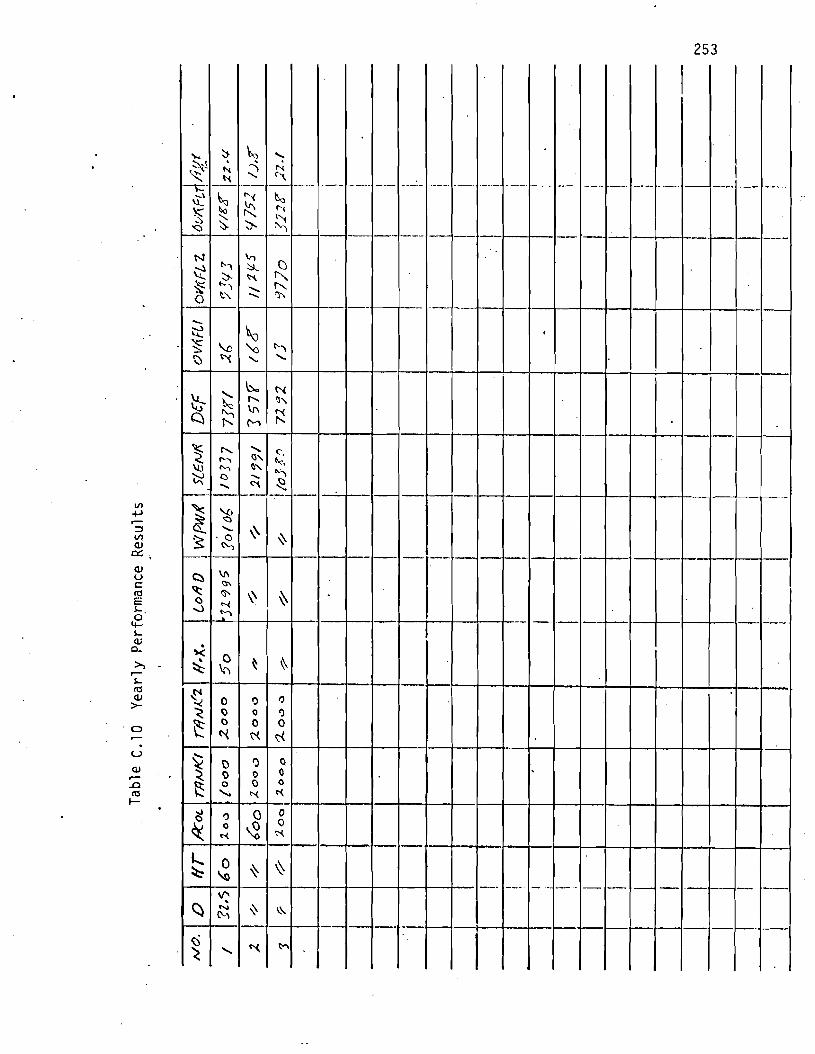
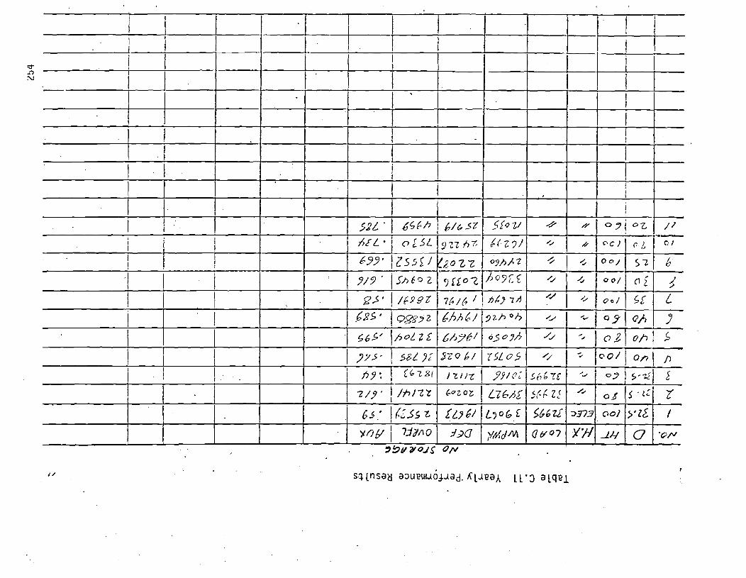
Table C.14 Yearly Econcmics Results -. - - - - ,

I n t . Rate= 0.08 LOAD- - ~ 2 9 3 5 Kv/h S t o r a g e = 2000 Gd//o*

No. Years= 20 H.W.= 0

do. I D

,' - I F t .

E l e c . Ann. Cost+Fue?+Furnace

-- HT I ACOL ! W X .

F t . ' r e s e n t F u t u r e

VO

,-132.5 , I

5 --.

Conv.

T o t a l C o s t S&w

P r e s e n t

Gas Ann. C ~ s t - i F u e l + 'urnace

F u t u r e

876 1798

i d 2 7

r

1 7 7 ~ 7 / 3 0

6

5021

60. 3 6 0 ) / ' . ? . 9 . 3

, , / / /(m0137.0 /i)~g.'o 5 ~ 5 0 /(/57 ( Y S ~ ? 5: 7 6 /500"

p,-; ./ /2:3

11 7 ' / / j ' t -.

f/n . , ( - ) { , ~ o . , 15.6 /6273 g /oL 9 , I / / o % > ,

7 2 32.5 4-0 l ; d 0 2 2 . / 135,'.; 62.76 1 7 ~ ~ l I 0 3 q j. 7; / 7 7 ~

Conv. Ann.

P r e s e n t

/ 0 3 9

P r e s e n t

14273

//?',':

3

F u t u r e

/ 5 9 /

l n d i /.,-**'

:17/

2 / 7 1

2,71

21 i /

;/,I A17i

.?/ / I

1 0 3 1 1 ,7? I / v L ~ 1 /~.t',5

' r <:I--' I r J ~ l A ~ c - l

972 1276

O i i Cost+Fuel+Furnace

- 7 ,:<33

9 5 ~ j 974 /,-?Z 1 / 0 5 3 / it74'

1#/7L/ > j . y

67.9 -- - I / /

I I I

I I - I

I i - I I.

/r73 1 J.?- 1 2 7 L

F u t u r e

974

' 1

1,~:;; 2 2 . 2 / 2 ;? ZV,O 112 ;q

l r j ' / I / ~ z / 2

---.

Conv.

/ d 7 q i 1 2,2/ , /,< q;

Y):, I / / g c

1

I

I

j I

t C / d

9- I i /

J

/24'"; 4 9 2 2 /,&)/5 1 / d ~ 5

!

I

1

$ i q 1/?56

I

-

r3 U1

I I

1

/^P&

i I I

'7 , ' to

j -4

I I

-

2/7/

,

/ 7 1 d

1

i-

2.171

1 .i;J 2 / 5 0 / / J 2 0 2

I 1 . I

Table C . 15 Yearly Economics Results. Int. Rate= C 8 LOAD= Mi92 A'jqb No. Years= 20 H.W.= 0

a-

HT ! ACOL ; AUX. ) Total Cost S&M Gas O i 1 El ec . Ann. Cost+ Fuel + Furnace Ann. Cost+Fuel+Furnace Ann. Cost+Fuel+Furnace

Present 1 Future ! Conv. 1 present l~uture I Conv. Iresent l~uture 1 Conv.