SEMANTICCNR/ISMARNTUA

Wind and Wave Atlas of the

Mediterranean Sea

Wind and Wave Atlas of the

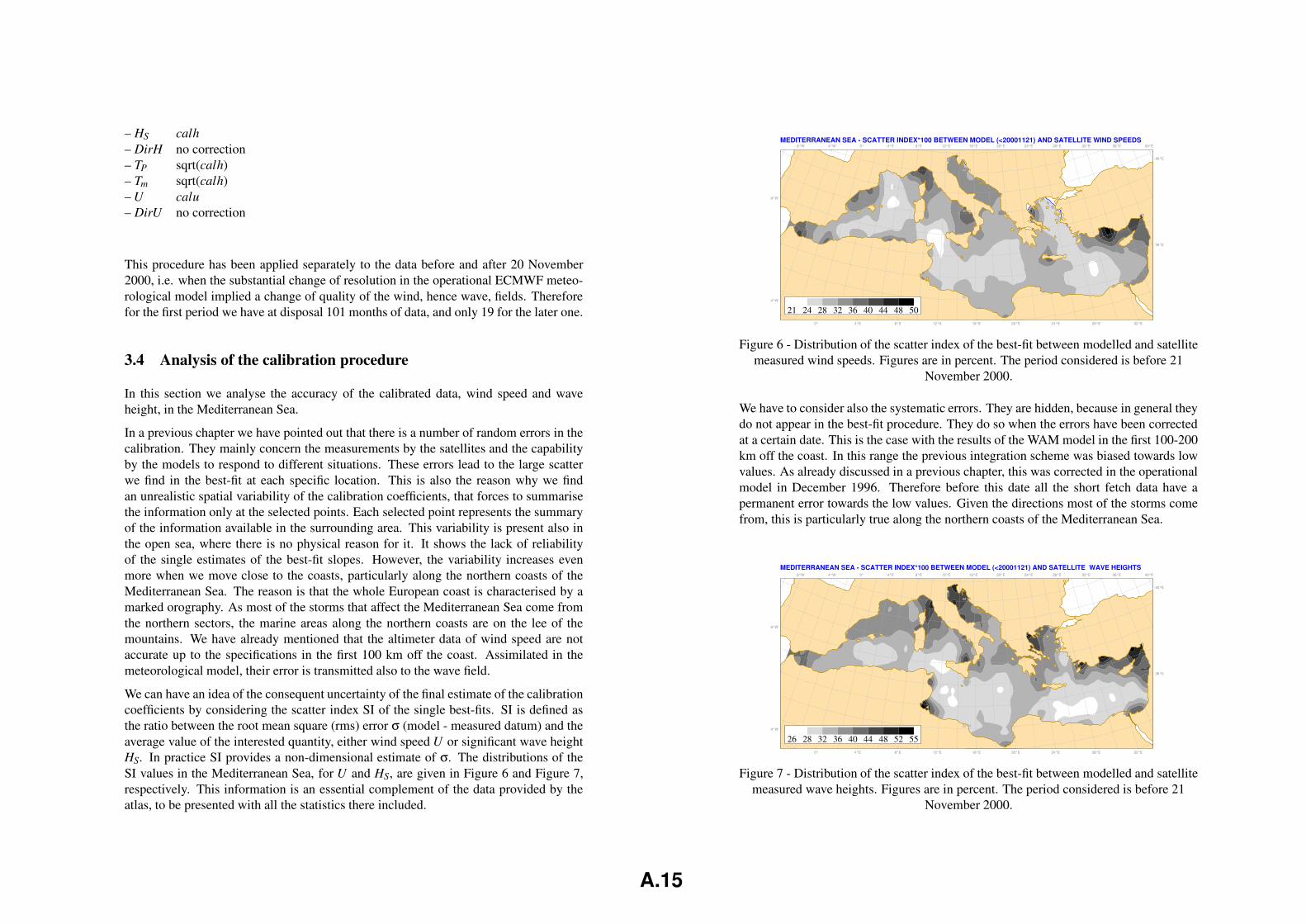
Mediterranean Sea

APRIL 2004

WESTERN EUROPEAN UNIONWESTERN EUROPEAN ARMAMENTS ORGANISATION

RESEARCH CELL

This page has been intentionally left BLANK

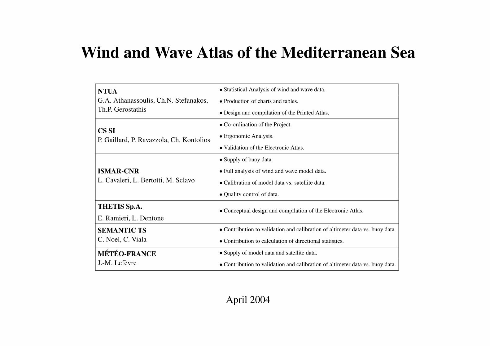
Wind and Wave Atlas of the Mediterranean Sea

NTUAG.A. Athanassoulis, Ch.N. Stefanakos,Th.P. Gerostathis

• Statistical Analysis of wind and wave data.

• Production of charts and tables.

• Design and compilation of the Printed Atlas.

CS SIP. Gaillard, P. Ravazzola, Ch. Kontolios

• Co-ordination of the Project.

• Ergonomic Analysis.

• Validation of the Electronic Atlas.

ISMAR-CNRL. Cavaleri, L. Bertotti, M. Sclavo

• Supply of buoy data.

• Full analysis of wind and wave model data.

• Calibration of model data vs. satellite data.

• Quality control of data.

THETIS Sp.A. • Conceptual design and compilation of the Electronic Atlas.E. Ramieri, L. Dentone

SEMANTIC TSC. Noel, C. Viala

• Contribution to validation and calibration of altimeter data vs. buoy data.

• Contribution to calculation of directional statistics.

METEO-FRANCEJ.-M. Lefevre

• Supply of model data and satellite data.

• Contribution to validation and calibration of altimeter data vs. buoy data.

April 2004

This page has been intentionally left BLANK

Foreword

General Introduction

It is obviously useful to have available a detailed and prolonged statistics of the wind andwave conditions in an area of interest. The WW-Medatlas project had the aim to pro-duce such an atlas for the Mediterranean Sea, making use of the data and methodologiespresently available.

Traditionally, extended wind and wave data in the open sea were available only from thevisual reports by sailors. Notwithstanding the strong limitations, several atlases havebeen built from this source. The actual measurement of the wave conditions at specificlocations became current practice with the introduction of the wave measuring buoys.Wind data in the open sea were more rare, as taken from special buoys or from open seaplatforms. Then the satellite era began, with a steady flow of wind and wave data. Atthe same time the numerical models, both meteorological and wave ones, improved theiraccuracy to a point where their results could be reliably used for practical purposes.

This may look like an overwhelming amount of data. However, each source has itsdrawbacks and limitations. The buoys are very sparse, and only a limited number ofthem are available. Each satellite moves along a fix orbit, and the altimeter derived dataare available only along its ground tracks, with large spaces between, at a time intervalequal to the duration of the cycle, typically between 10 and 30 days. The numericalmodels are the densest source, both in space and time. However, they are models, andas such only an approximation to the truth.

The solution lies in the combined use of all these sources, complementing their variousdrawbacks with the data from an alternative source. This has been the principle followedfor the preparation of this atlas.

Such a procedure is not straightforward and requires several steps. The data, both fromthe measurements and from the models, need to be collected, checked for possible

macroscopic errors and eventually corrected. Then the various sources must be com-bined, providing the final dataset suitable for the final statistics. This report describesthe overall procedure followed for the production of the atlas and the available results.

The present Atlas has been based on model data, appropriately calibrated by meansof satellite altimeter measurements. In that way the systematic space-time coverage, aunique feature of numerical models, is fully exploited and, at the same time, the qualityof the data and presented results is significantly improved by using the most up-to-dateand reliable measurement technique able to cover large sea areas: satellite remote sens-ing.

A 10-year data set consisting of 935 data points, distributed throughout the wholeMediterranean sea, has been collected, calibrated, analyzed and exploited in prepar-ing the Atlas. Various important statistical parameters have been calculated for the mainwind and wave characteristics, and their geographical distribution has been displayed,on a seasonal basis, by contour lines in 70 maps. Besides, 2580 bivariate histograms forthe main wind and wave characteristics have been calculated (again on a seasonal basis)and presented for 129 points along the Mediterranean Sea, in the printed Atlas. All theseresults (maps, contour lines and histograms) are also available in electronic form, pro-viding the user with additional, more flexible and more efficient, tools for treating andrecovering the information he/she needs. In the electronic Atlas, histograms and relatedstatistics are given for an extended set of 239 data points.

Neither measurements nor models are perfect. Therefore the user should not forget thatthe results here provided are only approximations of the truth. A detailed discussionof the accuracy of the results and of its geographical distribution is given in the text.However, we can confidently state that these are among the best data available in theMediterranean Sea. A well thought use of the atlas would be the key to make the best ofit.

Acknowledgements

The authors would like to thank:

– The Western European Union for their financial support,

– CNES (Centre National des Etudes Spatiales) and NASA (National Aeronauticand Space Agency) for having provided TOPEX altimeter data,

– ESA (European Space Agency) for having provided ERS altimeter data,

– the personnel of ECMWF for their help during the retrieval and the analysis of thewind and wave model data,

– Ente Publico Puertos del Estados, Clima Maritimo, Madrid, Spain,

– Ministry of Transport and Public Works, Sea Works Unit, Nicosia, Cyprus,

i

– National Center for Marine Research, Anavyssos, Greece, for providing with buoydata from their area of responsibility,

– Prof. I.V. Lavrenov, Arctic and Antarctic Research Institute, St. Petersburg, Rus-sia, for a preliminary hindcast study of the Greek Seas

Among the many other people that we want to acknowledge for their contribution andsupport, we mention:

– Kostas Belibassakis, Yannis Georgiou, Panagiotis Gavriliadis and Yanna Raptifrom NTUA for their support during the period 1999-2004

– A. Bergamasco who has contributed on Medatlas project as Thetis’s project man-ager during the first 2 years,

– Nathalie Imperatrice, engineer at CS SI, for her contribution for producing thetime series datasets of ten year length,

– Martine Pellen-Blin, Fabien Colomban, Philippe Cassou engineers at CS SI, forthe ergonomic evaluation and software validation of the Electronic atlas and forquality control on deliverables.

ii

Contents

Foreword . . . . . . . . . . . . . . . . . . . . . . . . . . . . . . . . . . . . i

A Theoretical Background A.1

1 Introduction . . . . . . . . . . . . . . . . . . . . . . . . . . . . . . . . A.1

1.1 Aim of the project and of the atlas . . . . . . . . . . . . . . . . A.1

1.2 General description of the atlas’s content . . . . . . . . . . . . A.1

1.3 General outline of the applicability of the atlas . . . . . . . . . A.1

1.4 Customers . . . . . . . . . . . . . . . . . . . . . . . . . . . . A.1

1.5 Partners . . . . . . . . . . . . . . . . . . . . . . . . . . . . . . A.2

2 Data sources . . . . . . . . . . . . . . . . . . . . . . . . . . . . . . . . A.5

2.1 Measured Data . . . . . . . . . . . . . . . . . . . . . . . . . . A.5

2.2 Model data . . . . . . . . . . . . . . . . . . . . . . . . . . . . A.8

2.3 Data handling . . . . . . . . . . . . . . . . . . . . . . . . . . . A.11

3 Calibration . . . . . . . . . . . . . . . . . . . . . . . . . . . . . . . . A.11

3.1 The data available for calibration . . . . . . . . . . . . . . . . . A.12

3.2 Choice of points . . . . . . . . . . . . . . . . . . . . . . . . . A.12

3.3 Calibration procedure . . . . . . . . . . . . . . . . . . . . . . . A.12

3.4 Analysis of the calibration procedure . . . . . . . . . . . . . . A.15

4 Statistical modelling and analysis of wind and waves . . . . . . . . . . A.17

4.1 Short term and long term statistical modelling of wind and waves A.17

4.2 Description of the data samples . . . . . . . . . . . . . . . . . A.18

4.3 From original samples to grouped samples . . . . . . . . . . . A.20

4.4 Analytic probability models . . . . . . . . . . . . . . . . . . . A.22

4.5 Wind and wave climate in the Mediterranean Sea . . . . . . . . A.23

5 Reliability assessment of the atlas . . . . . . . . . . . . . . . . . . . . A.27

5.1 Critical analysis of the reliability of the calibrated data . . . . . A.27

5.2 Geographical distribution of the reliability . . . . . . . . . . . . A.28

6 Electronic atlas . . . . . . . . . . . . . . . . . . . . . . . . . . . . . . A.28

6.1 Content of the electronic atlas . . . . . . . . . . . . . . . . . . A.28

6.2 Design and development of the electronic atlas . . . . . . . . . A.30

Bibliography . . . . . . . . . . . . . . . . . . . . . . . . . . . . . . . A.30

B Statistical Results B.1

1 Charts of mean wind speed . . . . . . . . . . . . . . . . . . . . . . . . B.3

2 Charts of wind direction . . . . . . . . . . . . . . . . . . . . . . . . . B.9

3 Charts of mean wave height . . . . . . . . . . . . . . . . . . . . . . . . B.15

4 Charts of mean wave period . . . . . . . . . . . . . . . . . . . . . . . B.21

5 Charts of mean wave slope . . . . . . . . . . . . . . . . . . . . . . . . B.27

6 Charts of wave direction . . . . . . . . . . . . . . . . . . . . . . . . . B.33

7 Charts of wind speed isopleths . . . . . . . . . . . . . . . . . . . . . . B.39

8 Charts of wave height isopleths . . . . . . . . . . . . . . . . . . . . . . B.61

9 Histograms of wind speed-wind direction . . . . . . . . . . . . . . . . B.83

10 Histograms of wave height-wave period . . . . . . . . . . . . . . . . . B.159

11 Histograms of wave height-wave direction . . . . . . . . . . . . . . . . B.235

12 Histograms of wave height-wind speed . . . . . . . . . . . . . . . . . . B.311

iii

This page has been intentionally left BLANK

iv

Part A

Theoretical Background

1 Introduction

1.1 Aim of the project and of the atlas

This atlas is the result of the Medatlas project led between 1999 and 2004 by a con-sortia of six companies located in France, Italy and Greece (see section 1.5 for furtherinformation). The main objective of this atlas is to provide reliable long term wind andwaves statistics at specified points of the Mediterranean Sea at pratically every offshorelocation (at about 50 km intervals).

1.2 General description of the atlas’s content

This atlas presents the results of the statistical analysis carried out on wind and wavedata, spanning a ten year period collected and analysed by the participants. These resultsare presented either in graphical form (charts) or in tabular form (bivariate histograms)which are described more in details in chapter 6.

1.3 General outline of the applicability of the atlas

The information contained in this Atlas can be used in various ways and for variousdifferent applications in Ship Design and Operational Planning, as well as in Offshoreand Coastal Engineering. Among them, we mention, as examples, the following:

– Operational Planning and Optimization of existing ships or fleetBy defining margins of operationally acceptable environmental conditions for ex-isting ships (single ship or a fleet), and using the information of the Atlas to assessprobabilities, it is possible to calculate operability indices, optimize the overallefficiency of ships, reorganise the geographical distribution of a fleet etc.

– Compare different designs by means of their operability indices

– Perform operational planning of offshore activities (naval or civil)

– Planning the seasonal window (e.g, month) of a war-at-sea exercise

– Planning the seasonal window of a specific offshore activity (hauling up,dredging, construction)

– Planning the most appropriate period for organizing a sailing race

– Ship DesignFor safety reasons, the key information is the extreme value of wind and waveparameters, which are not examined in this Atlas.For assessing the operability of a specific design in a specific sea environment wehave to study the efficiency/operability of this design in various sea states and theaverage by using the long-term probability of occurrence, which is provided bythe Atlas.

– Assess offshore wave energy resource

1.4 Customers

1.4.1 Western European Union - Research Cell

The current mission of the WEAO Research Cell is to provide the member nations ofthe WEAO with an efficient and effective service in the field of co-operative defenceresearch and technology.

WHAT IS THE WEAO?

The Western European Armaments Organisation (WEAO) was created in Ostend in Oc-tober 1996 by the adoption of its Charter and signature of the WEAO MOU by the then13 members of WEAG. Its membership has since increased to 19. It is a subsidiary bodyof the WEU and shares in the WEU’s legal personality Although the WEAO Charter andMOU are the foundation documents for the creation of an European Armaments Agency,the Organisation is currently operating only as a Research Cell, known usually by theacronym WRC. Its offices are in Brussels, co-located with the WEU Secretariat and theArmaments Secretariat of WEAG. The Cell is headed by a General Manager, plus 13members of staff, drawn from 8 different European countries. The General Manager isresponsible to the Board of Directors of the WEAO; the Board is currently made up ofthe National Armaments Directors of the 19 member states, and meets in formal sessionin March and October each year.

A.1

WHAT DOES THE WRC DO?

The WRC provides the WEAO member states with a variety of services in the field ofdefence Research and Technology. Some are common services provided to all members,whilst some support specific groups of nations undertaking co-operative R&T projects.

The common services provided by the WRC include administrative support to theWEAO Board of Directors and the WEAG Panel II (the Research and Technology Panelof WEAG), and to their subsidiary groups and committees, and advice to WEAO mem-bers on a variety of matters to do with R&T co-operation. Collectively, the staff of theCell have expertise in a wide variety of subjects; they include not only scientists, engi-neers and contracts specialists, but also staff who are expert in IT, in MOU and generallegal matters, in organisation and management of conferences, and of course in gen-eral administration in an international context. The WRC supports co-operative R&Tprojects by assisting the participating nations to prepare and sign the relevant project ar-rangements, by providing administrative support to the project management teams whenrequired, and by letting contracts for research work on behalf of the project participants.The Cell is able to let contracts using the legal personality of the WEU.

1.4.2 Delegation Generale pour l’Armement (France)

Established in April 1961 within the Ministry of Defence, the Delegation Generale pourl’Armement (DGA) prepares future defence capabilities and runs the development ofmaterials as well as weapon systems to equip French Armed Forces.

DGA is in charge of designing and acquiring weapon systems to meet the needs ex-pressed by Armed Forces. As such, it is tasked with preparing tomorrow’s defenceequipment and conducting armament programmes. DGA runs its activities in partner-ship with the headquarters staff, the users of equipment thus developed, and with arma-ment industrialists who manufacture the equipment.

DGA’s added value lies in its high level of technical skills as well as its ability to con-trol risks involved in conducting particularly complex projects. DGA’s position withinthe Ministry of Defence makes it a privileged representative able to provide an overall“joint-service” view. As a result, DGA has been offering France a chance to acquirehigh technology materials and weapons such as the Leclerc tank, the Charles-de-GaulleAircraft carrier and the Rafale aircraft.

1.4.3 The Ministry of Defence of the Republic of Italy

The Ministry of Defence of the Republic of Italy was officially established in May 1947,after the reunification of the earliest Ministries of the War, Navy and Air Force. TheMinister of Defence is charged with implementation of security and defence guidelinesestablished by the Government and approved by the Parliament. Being advised by the

Chief of Defence Staff and the Secretary General of Defence/National Armaments Di-rector, the Minister defines the guidelines related to military policy, intelligence andsecurity, and technical/administrative activities.

The Secretary General of Defence/National Armaments Director is responsible for orga-nization and management of technical, industrial and administrative Defence areas. Heis also responsible for the activities of the Ministry of Defence related to research, devel-opment and procurement. Medatlas project (RTP10.10) has been managed and fundedas part of these activities.

1.4.4 Hellenic Ministry of National Defence / General Secretariat for EconomicPlanning and Defence Investments

The Ministry of Defence (MoD) and the Hellenic Armed Forces under its command(Army, Navy, Air Force), implement the National Defence Policy decided upon by theHellenic Government.

The Ministry of Defence focuses on issues related to defence policy, national defencedesign and planning, the structure of the Armed Forces, crisis management and the eval-uation of intelligence material. In addition, relations with international organisations,personnel training and welfare, infrastructure and armaments, conscript recruitment pol-icy, information technology and meteorology, as well as the social contribution of theArmed Forces, constitute major areas of MoD activity.

The General Secretariat for Economic Planning and Defence Investments is a separatebody of the MoD, which supports the Minister in the areas of economic planning andbudgeting, the implementation of armaments programs and expenditures, military com-pensatory benefits, the development of domestic defence industry and technology, andthe optimal utilisation of the real estate portfolio of the National Defence Fund.

1.5 Partners

1.5.1 CS

CS (or CS SI) is positioned at the crossroads of information and communications sys-tems, infrastructure installations and scientific and technical applications for both civil-ian and military use. Its comprehensive range of services includes systems design, inte-gration and outsourcing. Nearly 70% of CS’s work involves projects that span severalyears. CS builds long-term relationships with its customers and provides them with thesolutions that are best suited to their needs and resources.

As MedAtlas Project SLIE (Single Legal Industrial Entity), CS has represented IEs (In-dustrial Entities) in front of Research and Technology Project (RTP) Research Cell (RC)and Management Group (MG). As such, CS was responsible for the overall project man-agement and helds the interface to the MG for all administrative and technical aspects

A.2

of the MEDATLAS project. Responsible for carrying out the MedAtlas project in goodconditions and as official interlocutor of the MG for the contract execution, CS has beenspecially in charge of:

– Contract management, and technical control for the Work Packages (WPs),

– MG consultation for every request of the project evolution,

– Co-ordination in Consortium,

– In collaboration with each IE, technical progresses assessment of each WP andreporting towards the MG,

– Meetings preparation and leading.

In addition, CS has taken part in:

– Data base creation, loading and administration,

– Ergonomic evaluation and software validation of the Electronic atlas,

– Data migration in order to provide not calibrated data in time series format for allthe 935 points and ten years period.

1.5.2 NTUA

NATIONAL TECHNICAL UNIVERSITY of ATHENS (NTUA) is the oldest technicaluniversity in Greece, covering all disciplines of engineering. The University is dividedinto nine academic departments and operates about a hundred laboratories within thesphere of its technological competence.

The School of Naval Architecture and Marine Engineering, which is one of the mostactive departments at NTUA, consists of four Divisions and operates four Laborato-ries. In the Division of Ship and Marine Hydrodynamics, the Sea Wave Research Groupis being involved, through academic research and European and National projects, inresearch concerning wave modelling and wave transformation, wave-body interactionproblems, coastal hydrodynamics, ocean wave statistics, stochastic modelling of waveclimate, wave energy, remote sensing, marine geographical information systems, inte-grated graphical user interfaces for marine/coastal applications, and marine atlases bothin electronic and paper form.

The main contributions of NTUA in the present project are:

– the systematic derivation of long-term wind and wave statistics, including empiri-cal probability densities and the appropriate probabilistic modelling of the variousparameters studied (univariate, bivariate, directional, time series),

– the systematic production of charts and tables for the various wind & wave pa-rameters, and

– the design, realisation and publication of the Printed form of the atlas, includingthe design of the cover page.

Apart from the above major contributions, NTUA has also contributed to:

– the collection of in situ measurements,

– the development of the user-interface,

– the design and development of graphical presentation software,

– the testing and validation of the Electronic version of the atlas.

1.5.3 ISMAR

One of the largest institutes of CNR, the Italian National Research Council, ISMAR(formerly ISDGM) has three main lines of activity, devoted respectively to the studyof coastal areas and lagoons, geology and oceanography. Within the last section, nu-merical modelling has a prominent role, focused on circulation and wave modelling, inboth deep and shallow water. While ISMAR has no operational role, the institute hascontributed to the development and implementation of many operational models in Italyand abroad.

Given its previous experience, the main role of ISMAR in this project was the partlyretrieval, the handling and calibration of the ECMWF wind and wave data. Ten years ofdata have been screened and homogenised to take into account the changes occurred inthe models during the whole period. The data, available as fields, have been transformedinto time series at each of the points chosen for late consideration in the atlas.

The satellite data provided by Meteo-France have been prepared for comparison withmodel data. The distribution of co-located values have been carefully analysed withsophisticated statistical tools deriving correction coefficients for both wind and wavemodel parameters at each chosen location. These coefficients have been analysed forconsistency and used to obtain the final calibrated model results.

ISMAR has done a critical analysis of the errors present in the model and satellite data,and derived an estimate of the accuracy of the calibrated data and of its geographicaldistribution. It has provided the wave data for the Italian network, to be used for theassessment of the quality of the altimeter data. It has also used these data for an assess-ment of the performance of the ECMWF wind and wave models in the MediterraneanSea. ISMAR has carried out statistics for the wind and wave model data, estimating inparticular the dominant wind and wave directions at the single grid points and the spatialvariability of the overall fields.

A.3

1.5.4 THETIS

Thetis is a Technological Centre based in the historic Arsenale of Venice. Thetis op-erates as a systems integrator in the development of projects, services and innovativetechnological applications in two business areas:

– Environmental and civil engineering:

– System analysis; specialist and environmental impact studies; environmentalmonitoring systems and services; environmental informatics; dissemination oftechnical and scientific information.

– Facility management; restoration and rehabilitation of historic buildings; tech-nologies for urban maintenance; structural integrity monitoring systems; projectmanagement.

– Intelligent Transport Systems (ITS)

– GPS localisation and fleet management systems and services for public transportapplications; maritime and inland navigation management systems (VTMIS, Ves-sel Traffic Management Information Services).

The main contribution of Thetis in MedAtlas project was to develop the electronic ver-sion of the Mediterranean wind and wave atlas. This activity initially concentrated onthe conceptual design of the electronic application and the definition of its general archi-tecture. Afterward Thetis developed the electronic atlas interface and produced differentapplication releases. These were evaluated by customers and partners, as well as sub-jected to specific ergonomic analyses and validation plans.

Finally, Thetis integrated data (bivariate frequency tables, spatial distribution of statisti-cal quantities, spatial distribution of probabilities of important events) in the electronicatlas and performed an accurate final evaluation.

The software MapObject version LT of the ESRI family was used to develop the elec-tronic atlas.

1.5.5 SEMANTIC TS

SEMANTIC-TS is a French SME specialized in research and development, from de-velopment of physical idea and its mathematical modelling, to implementation of insitu measurement or signal processing system. Semantic TS company conducts stud-ies, develops specific softwares, and organizes measurement campaigns in the areas ofoceanography, time-frequency domain, underwater acoustics, environment and signalprocessing.

Contribution of SEMANTIC TS remains first in calculating directional statistics of wavedata and building a tool for NTUA’s analyses of the data. WAM hindast wave data havebeen made available and processed and directional statistics have been calculated (polarhistogram and wave rose). Results have been presented in a web site which constitutes auseful tool because it gathers, in a unique site, observable in any computer environment,all the available information which was in different formats. This allowed facilities toanalyze data and synthesize results.

On a second hand, SEMANTIC TS has used available buoys and altimeters wave datain the Mediterranean Sea for a validation and calibration of altimeter data. Data from15 Mediterranean buoys and from Topex and ERS satellites have been collected andprocessed, in order to create collocation files and show comparison statistics. Colloca-tion results web sites have been computed as well as a sensibility study, and analysed incollaboration with METEO FRANCE.

1.5.6 METEO FRANCE

Meteo-France, a public administration placed under the authority of the Ministry ofTransport and Housing, is the French organisation responsible for supplying informationnationwide on the state of the atmosphere, of the ocean upper layer and the repercus-sions this may have on human life and property. Meteo-France is also a member stateof the European Centre for Medium-Range Weather Forecasting (ECMWF). Among thenecessary activities to meet these requirements, Meteo-France, receives, processes andarchives information supplied by observing systems, among them one finds polar orbit-ing environment satellites. Meteo-France also analyses all this information and feedsit into numerical prediction models, either at global scale or over areas of particularinterest.

As a meteorological service, the main contribution of Meteo-France in this project wasto collect data from numerical weather prediction models, from numerical wave predic-tion models and from satellite altimeters and scatterometers, for a ten years period forthe whole Mediterranean sea.

Then, because of its experience in using satellite data for improving and validating wavemodel analyses, Meteo-France was is charge of the validation/calibration of the satel-lite data that have been used to correct the model data. Among the wave models in theMediterranean sea, the most extended source is provided by ECMWF. The ERS near realtime data (Fast Delivery Products) from the European Space Agency (ESA) have beenarchived at Meteo-France. The TOPEX/Poseidon Geophysical Data Records (GDR’s)have been provided by CNES, the French space agency. Once validated and calibratedusing results from global studies, the altimeters wave data have been validated for theMediterranean Sea using buoys data collected for the project, in collaboration with SE-MANTIC TS.

A.4

2 Data sources

There are four main sources of marine wind and wave data available to the user:

– visual observations from ships,

– data measured from buoys or platforms,

– data measured by remote instruments on board of high altitude flying satellites,

– meteorological and wave models operational at the various meteo-oceanographiccentres.

These data have different characteristics expressed as quality, accuracy, errors present inthe data, geographical distributions, number of data. In the following sections we givea brief description of the data and of their use when assembling the atlas. In particu-lar we list also the problems and consequent limitations associated to each source andinstrument.

Remark about visual estimates:

Taken from ships of opportunity, this has been for a long time the only source of in-formation for wind and wave data in the open sea. Many decades of data exist, anda full generation of atlases has been based on these data. However, careful compar-isons with properly measured data have shown the limitations of this approach and thesubstantial errors potentially present in the reported data, particularly in stormy con-ditions, the situation that users care more about. From the point of view of the atlasof a full basin, a major limitation of the visual data is given by their preferential dis-tribution along the most common maritime routes, and by the tendency of the ships toavoid the stormy areas, in so doing substantially biasing the statistics that can be de-rived. Given the large availability of alternative data, that, combined in an optimal way(see later sections), provide a good accuracy and a complete coverage in space and time,no use has been made of visual estimates in the preparation of this atlas.

2.1 Measured Data

2.1.1 Buoy data

Introduction This has become since a while ago the standard method for the collec-tion of wave data in the open sea. The data are measured from a floating buoy, mooredat a given location. The local depth can reach a few hundreds metres, with the exclusionof very shallow water (a few metres).

The data The most common supplier of this kind of buoys has been Datawell, fromNetherlands. The first buoy was the Waverider, a surface following sphere including astabilised vertical accelerometer. The related signal is transmitted to land on a continu-ous basis, where it is recorded at predetermined intervals. The limit of this buoy is itscapability of measuring only the vertical component of motion of the surface. Hence nodirectional information is available.

The Waverider was followed by the Wavec, a much larger version with the capability ofrecording also directional information. Also this buoy is based on the principle of sur-face following. Therefore measuring the motion of the buoy corresponds to know howthe local geometrical characteristics of the sea surface change with time. The physicalquantities measured are the surface elevation and the two orthogonal components of thesurface slope. Proper mathematical handling of these quantities provides estimate ofthe elevation frequency spectrum, and of the dependence on frequency of mean wavedirection, skewness and kurtosis. Further integration leads to the integral parameterssignificant wave height HS, mean direction θm, peak and mean period TP and Tm.

The Wavec buoy is quite large, its overall diameter, once assembled, measuring morethan 3 metres. The weight is more than 700 kg. While this poses obvious difficulties forits handling, it is also a deterrent to the improper removal or damaging of the buoy. Asthe Waverider, the Wavec buoy is characterised by a very high reliability. During morethan ten years of operation in the network around Italy (RON, De Boni et al., 1993) thedata obtained amount to more than 90% of the theoretical maximum. The interruptionshave been due mainly to software problems in the transmission of the data from the landstation to the central collection office.

As the Waverider, the Wavec buoy is continuously in operation, i.e. the signal carry-ing the measurements is continuously transmitted. The sequence of recording is purelya strategic decision, based on a trade-off between the information made available, theamount of repetitive information and the associated volume of storage. In general athree-hour interval is chosen between two sequential records, to be taken at synoptictimes (00, 03, 06, . . . UT), to be eventually reduced in case of a severe storm. In morerecent times the Wavec has been progressively substituted by the Directional Waverider,a much lighter version still with directional capabilities.

A substantial number of these buoys, either Waverider or Wavec or Directional Wa-verider, are distributed along the coasts of the Mediterranean Sea. A summary of thesituation, including the satellite data discussed in the next section, is given in Table 1.The Table provides the location, its geographical coordinates, the local depth, and theperiod for which the data were available for this project. The most substantial sourceof buoy data was given by the Italian network RON (De Boni et al., 1993). However,a large network exists also along the Spanish coastline. Table 2 lists the informationavailable from the single sources.

A.5

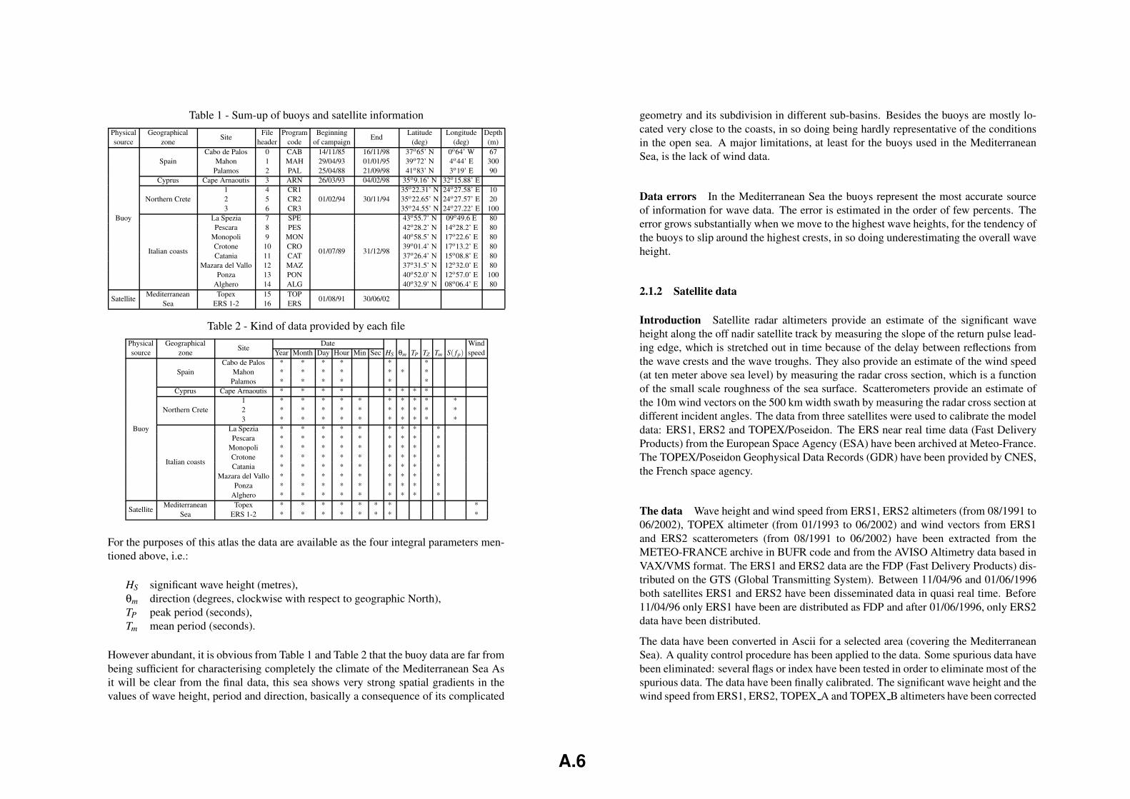
Table 1 - Sum-up of buoys and satellite informationPhysical Geographical

SiteFile Program Beginning

EndLatitude Longitude Depth

source zone header code of campaign (deg) (deg) (m)

Buoy

SpainCabo de Palos 0 CAB 14/11/85 16/11/98 37o65’ N 0o64’ W 67

Mahon 1 MAH 29/04/93 01/01/95 39o72’ N 4o44’ E 300Palamos 2 PAL 25/04/88 21/09/98 41o83’ N 3o19’ E 90

Cyprus Cape Arnaoutis 3 ARN 26/03/93 04/02/98 35o9.16’ N 32o15.88’ E

Northern Crete1 4 CR1

01/02/94 30/11/9435o22.31’ N 24o27.58’ E 10

2 5 CR2 35o22.65’ N 24o27.57’ E 203 6 CR3 35o24.55’ N 24o27.22’ E 100

Italian coasts

La Spezia 7 SPE

01/07/89 31/12/98

43o55.7’ N 09o49.6 E 80Pescara 8 PES 42o28.2’ N 14o28.2’ E 80

Monopoli 9 MON 40o58.5’ N 17o22.6’ E 80Crotone 10 CRO 39o01.4’ N 17o13.2’ E 80Catania 11 CAT 37o26.4’ N 15o08.8’ E 80

Mazara del Vallo 12 MAZ 37o31.5’ N 12o32.0’ E 80Ponza 13 PON 40o52.0’ N 12o57.0’ E 100

Alghero 14 ALG 40o32.9’ N 08o06.4’ E 80

SatelliteMediterranean

SeaTopex 15 TOP

01/08/91 30/06/02ERS 1-2 16 ERS

Table 2 - Kind of data provided by each filePhysical Geographical

SiteDate Wind

source zone Year Month Day Hour Min Sec HS θm TP TZ Tm S( fp) speed

Buoy

SpainCabo de Palos * * * * * *

Mahon * * * * * * *Palamos * * * * * *

Cyprus Cape Arnaoutis * * * * * * * *

Northern Crete1 * * * * * * * * * *2 * * * * * * * * * *3 * * * * * * * * * *

Italian coasts

La Spezia * * * * * * * * *Pescara * * * * * * * * *

Monopoli * * * * * * * * *Crotone * * * * * * * * *Catania * * * * * * * * *

Mazara del Vallo * * * * * * * * *Ponza * * * * * * * * *

Alghero * * * * * * * * *

SatelliteMediterranean

SeaTopex * * * * * * * *

ERS 1-2 * * * * * * * *

For the purposes of this atlas the data are available as the four integral parameters men-tioned above, i.e.:

HS significant wave height (metres),θm direction (degrees, clockwise with respect to geographic North),TP peak period (seconds),Tm mean period (seconds).

However abundant, it is obvious from Table 1 and Table 2 that the buoy data are far frombeing sufficient for characterising completely the climate of the Mediterranean Sea Asit will be clear from the final data, this sea shows very strong spatial gradients in thevalues of wave height, period and direction, basically a consequence of its complicated

geometry and its subdivision in different sub-basins. Besides the buoys are mostly lo-cated very close to the coasts, in so doing being hardly representative of the conditionsin the open sea. A major limitations, at least for the buoys used in the MediterraneanSea, is the lack of wind data.

Data errors In the Mediterranean Sea the buoys represent the most accurate sourceof information for wave data. The error is estimated in the order of few percents. Theerror grows substantially when we move to the highest wave heights, for the tendency ofthe buoys to slip around the highest crests, in so doing underestimating the overall waveheight.

2.1.2 Satellite data

Introduction Satellite radar altimeters provide an estimate of the significant waveheight along the off nadir satellite track by measuring the slope of the return pulse lead-ing edge, which is stretched out in time because of the delay between reflections fromthe wave crests and the wave troughs. They also provide an estimate of the wind speed(at ten meter above sea level) by measuring the radar cross section, which is a functionof the small scale roughness of the sea surface. Scatterometers provide an estimate ofthe 10m wind vectors on the 500 km width swath by measuring the radar cross section atdifferent incident angles. The data from three satellites were used to calibrate the modeldata: ERS1, ERS2 and TOPEX/Poseidon. The ERS near real time data (Fast DeliveryProducts) from the European Space Agency (ESA) have been archived at Meteo-France.The TOPEX/Poseidon Geophysical Data Records (GDR) have been provided by CNES,the French space agency.

The data Wave height and wind speed from ERS1, ERS2 altimeters (from 08/1991 to06/2002), TOPEX altimeter (from 01/1993 to 06/2002) and wind vectors from ERS1and ERS2 scatterometers (from 08/1991 to 06/2002) have been extracted from theMETEO-FRANCE archive in BUFR code and from the AVISO Altimetry data based inVAX/VMS format. The ERS1 and ERS2 data are the FDP (Fast Delivery Products) dis-tributed on the GTS (Global Transmitting System). Between 11/04/96 and 01/06/1996both satellites ERS1 and ERS2 have been disseminated data in quasi real time. Before11/04/96 only ERS1 have been are distributed as FDP and after 01/06/1996, only ERS2data have been distributed.

The data have been converted in Ascii for a selected area (covering the MediterraneanSea). A quality control procedure has been applied to the data. Some spurious data havebeen eliminated: several flags or index have been tested in order to eliminate most of thespurious data. The data have been finally calibrated. The significant wave height and thewind speed from ERS1, ERS2, TOPEX A and TOPEX B altimeters have been corrected

A.6

according to relations deduced from comparisons with buoys measurements, cross com-parisons between altimeters, and global analyses of the evolution of the significant waveheight (SWH).

Calibration of the data

1/ Topex data The significant wave height and the wind speed from TOPEX altime-ter have been corrected according to relations deduced from comparisons with buoysmeasurements (Cotton et al, 1997, Lefevre and Cotton 2001).

SWHcor. = 1.052 SWHgdr−0.094U10cor. = 0.87 U10gdr +0.68

For TOPEX data, linear time dependant correction has been applied to the Ku band datain order to correct a maximum bias of 40 cm for cycle 236 (31/01/1999), starting fromno correction at cycle 132.

2/ ERS altimeter data The following regression relation, from Queffeulou (1994), hasbeen used to correct the SWH f dp for ERS1:

SWHcor. = 1.32 SWH f dp−0.72

For the ERS-2 SWH f dp, the following regression relation from Queffeulou (1996) hasbeen applied:

SWHcor. = 1.09 SWH f dp−0.12

Validation Once the satellite data were calibrated using results from global studies,a further validation of altimeter data in the Mediterranean Sea has been done using thelocally available buoys and altimeters wave data. The aim was to compare data frombuoys and satellites. As there is no data about wind speed from buoys, only HS has beencompared. To make the comparison possible, a collocation procedure (time and space)is needed. Obviously this can be done only with a certain approximation. The closerthey are, the most significant is the comparison. The comparison can be done with dif-ferent approximations in time (T ) and space (D), and for different ranges of wave height(H). Then T , D and H can be considered as parameters.

Data from 15 Mediterranean buoys and from Topex and ERS satellites have been col-lected and processed. Tools adapted to collocation files creation and analysis have beenfirst developed. That means:

• a database containing all the data

• a tool able to realise collocation on buoys and satellite data: that means to enhancecomparable data with different set of the parameters T , D and H

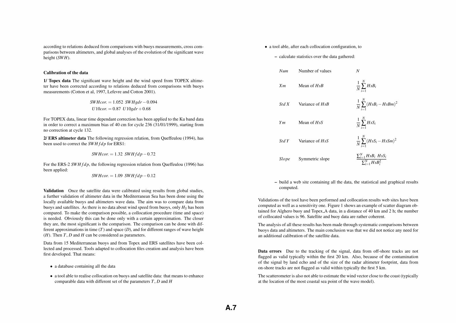
• a tool able, after each collocation configuration, to

– calculate statistics over the data gathered:

Num Number of values N

Xm Mean of HsB1N

N

∑i=1

HsBi

Std X Variance of HsB1N

N

∑i=1

(HsBi−HsBm)2

Y m Mean of HsS1N

N

∑i=1

HsSi

Std Y Variance of HsS1N

N

∑i=1

(HsSi−HsSm)2

Slope Symmetric slope∑N

i=1 HsBi HsSi

∑Ni=1 HsB2

i

– build a web site containing all the data, the statistical and graphical resultscomputed.

Validations of the tool have been performed and collocation results web sites have beencomputed as well as a sensitivity one. Figure 1 shows an example of scatter diagram ob-tained for Alghero buoy and Topex A data, in a distance of 40 km and 2 h; the numberof collocated values is 96. Satellite and buoy data are rather coherent.

The analysis of all these results has been made through systematic comparisons betweenbuoys data and altimeters. The main conclusion was that we did not notice any need foran additional calibration of the satellite data.

Data errors Due to the tracking of the signal, data from off-shore tracks are notflagged as valid typically within the first 20 km. Also, because of the contaminationof the signal by land echo and of the size of the radar altimeter footprint, data fromon-shore tracks are not flagged as valid within typically the first 5 km.

The scatterometer is also not able to estimate the wind vector close to the coast (typicallyat the location of the most coastal sea point of the wave model).

A.7

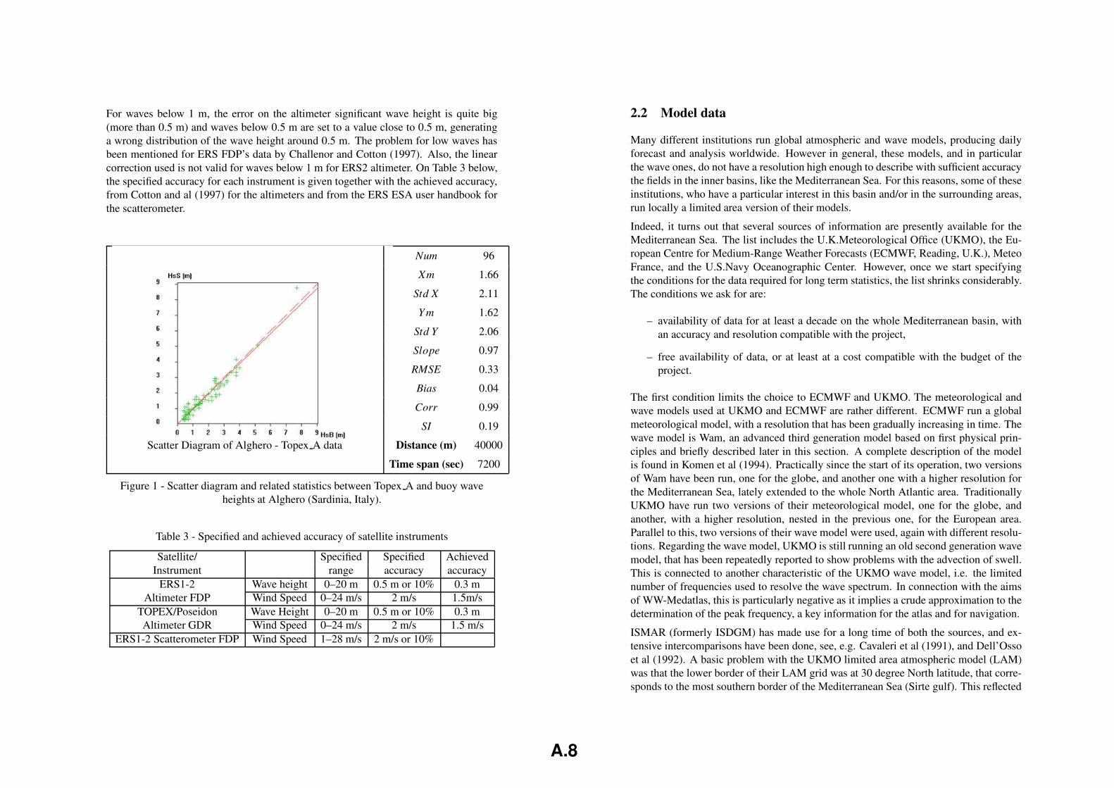
For waves below 1 m, the error on the altimeter significant wave height is quite big(more than 0.5 m) and waves below 0.5 m are set to a value close to 0.5 m, generatinga wrong distribution of the wave height around 0.5 m. The problem for low waves hasbeen mentioned for ERS FDP’s data by Challenor and Cotton (1997). Also, the linearcorrection used is not valid for waves below 1 m for ERS2 altimeter. On Table 3 below,the specified accuracy for each instrument is given together with the achieved accuracy,from Cotton and al (1997) for the altimeters and from the ERS ESA user handbook forthe scatterometer.

Num 96

Xm 1.66

Std X 2.11

Y m 1.62

Std Y 2.06

Slope 0.97

RMSE 0.33

Bias 0.04

Corr 0.99

SI 0.19

Scatter Diagram of Alghero - Topex A data Distance (m) 40000

Time span (sec) 7200

Figure 1 - Scatter diagram and related statistics between Topex A and buoy waveheights at Alghero (Sardinia, Italy).

Table 3 - Specified and achieved accuracy of satellite instruments

Satellite/ Specified Specified AchievedInstrument range accuracy accuracy

ERS1-2Altimeter FDP

Wave height 0–20 m 0.5 m or 10% 0.3 mWind Speed 0–24 m/s 2 m/s 1.5m/s

TOPEX/PoseidonAltimeter GDR

Wave Height 0–20 m 0.5 m or 10% 0.3 mWind Speed 0–24 m/s 2 m/s 1.5 m/s

ERS1-2 Scatterometer FDP Wind Speed 1–28 m/s 2 m/s or 10%

2.2 Model data

Many different institutions run global atmospheric and wave models, producing dailyforecast and analysis worldwide. However in general, these models, and in particularthe wave ones, do not have a resolution high enough to describe with sufficient accuracythe fields in the inner basins, like the Mediterranean Sea. For this reasons, some of theseinstitutions, who have a particular interest in this basin and/or in the surrounding areas,run locally a limited area version of their models.

Indeed, it turns out that several sources of information are presently available for theMediterranean Sea. The list includes the U.K.Meteorological Office (UKMO), the Eu-ropean Centre for Medium-Range Weather Forecasts (ECMWF, Reading, U.K.), MeteoFrance, and the U.S.Navy Oceanographic Center. However, once we start specifyingthe conditions for the data required for long term statistics, the list shrinks considerably.The conditions we ask for are:

– availability of data for at least a decade on the whole Mediterranean basin, withan accuracy and resolution compatible with the project,

– free availability of data, or at least at a cost compatible with the budget of theproject.

The first condition limits the choice to ECMWF and UKMO. The meteorological andwave models used at UKMO and ECMWF are rather different. ECMWF run a globalmeteorological model, with a resolution that has been gradually increasing in time. Thewave model is Wam, an advanced third generation model based on first physical prin-ciples and briefly described later in this section. A complete description of the modelis found in Komen et al (1994). Practically since the start of its operation, two versionsof Wam have been run, one for the globe, and another one with a higher resolution forthe Mediterranean Sea, lately extended to the whole North Atlantic area. TraditionallyUKMO have run two versions of their meteorological model, one for the globe, andanother, with a higher resolution, nested in the previous one, for the European area.Parallel to this, two versions of their wave model were used, again with different resolu-tions. Regarding the wave model, UKMO is still running an old second generation wavemodel, that has been repeatedly reported to show problems with the advection of swell.This is connected to another characteristic of the UKMO wave model, i.e. the limitednumber of frequencies used to resolve the wave spectrum. In connection with the aimsof WW-Medatlas, this is particularly negative as it implies a crude approximation to thedetermination of the peak frequency, a key information for the atlas and for navigation.

ISMAR (formerly ISDGM) has made use for a long time of both the sources, and ex-tensive intercomparisons have been done, see, e.g. Cavaleri et al (1991), and Dell’Ossoet al (1992). A basic problem with the UKMO limited area atmospheric model (LAM)was that the lower border of their LAM grid was at 30 degree North latitude, that corre-sponds to the most southern border of the Mediterranean Sea (Sirte gulf). This reflected

A.8

the focus of interest of UKMO on the British Isles. The problem lies in the boundaryconditions at the outer border of a LAM grid. At this position they are coincident withthe local ones from the global model. A LAM shows its power (more defined detailsof the fields, typically higher wind speeds, etc.) in the inner part of its grid. There-fore, while the UKMO LAM achieved its aim on UK, it was not so effective on theMediterranean Sea, particularly in its most southern part.

In the long term, but in any case within the first part of the last decade, the ISMAR expe-rience has been that, notwithstanding the different resolutions, the quality of the productsfrom the two centres was comparable, with possibly a better capability by ECMWF tocarve out details of the fields. After this period a direct comparison in the MediterraneanSea has not been a straightforward matter, due to the heavy commercialisation put onby UKMO. Using a three-year long intercomparison among different wind and wavemodels Bidlot et al (2001) found the following results between UKMO and ECMWF:

– the results for wind speed are quite similar,

– UKMO has a slightly smaller bias for wave height, but with a larger scatter,

– UKMO has by far the worst results for TP, because of the smaller number of fre-quencies considered.

On top of this, UKMO make available their products for a fee much higher than the onerequested by ECMWF. All the above conditions have led to the final choice of ECMWFas official source for the data to be used for the atlas. In the following paragraphs wegive a brief description of the models used at the Centre and of the available results.

2.2.1 The atmospheric model - wind data

The operational model at ECMWF is spectral, i.e. the horizontal fields are describedby a two-dimensional expansion of spherical harmonics truncated at, e.g., 319 (T319).The truncation identifies the resolution, here defined as half the smallest resolved wavelength, used to describe the fields. For T319 it is 40,000/(2 x 319)∼=63 km. Advection iscalculated with a semi-Lagrangian scheme, while the physics is carried out on a reducedGaussian grid in physical space. The vertical structure of the atmosphere is described bya multi-level hybrid σ coordinate system. The physical parameterisations describe thebasic physical processes connected to radiative transfer, turbulent mixing, subgrid-scaleorographic drag, moist convection, clouds and surface soil processes. The prognos-tic variables include wind components, temperature, specific humidity, liquid/ice watercontent and cloud fraction. Parameterisation schemes are necessary in order to properlydescribe the impact of subgrid-scale mechanisms on the large scale flow of the atmo-sphere. Forecast weather parameters, such as the two-metre temperature, precipitationand cloud cover, are computed by the physical parameterisation of the model. The ten

metre wind is derived with a boundary layer model from the lowest σ level, 0.997, cor-responding to about 30 metre height. A compact description of the model can be foundin Simmons (1991) and Simmons et al (1995).

The horizontal resolution and the number of levels with which the atmosphere is de-scribed in the model has varied in time. T213 (95 km resolution) and 31 levels wereused from 1991 till 1998, when ECMWF passed to T319. This change had a limited ef-fect, because the Gaussian grid , used to model the processes in physical space, was notchanged. The big step ahead came in November 2000, when the Centre passed to T511(about 40 km resolution), with 60 levels on the vertical and a 40 km resolution Gaus-sian grid. Cavaleri and Bertotti (2003a) have clearly shown how a different resolutionimplies a different quality of the results. In the Mediterranean Sea this corresponded toan appreciable increase of the wind speeds, a fact to be considered in the evaluation ofthe calibrated data and of the final statistics.

Errors The model data at very low wind speeds are not reliable because the situationis dominated by sub-grid processes. This is particularly true close to land, an obviousexample being the land-sea breezes.

In the coastal areas the model winds are unreliable in all the conditions because of thedominant influence of orography, not properly represented in the meteorological modelbecause of limited resolution (95 km for T213, 40 km for T511). Also the limited ac-curacy with which the actual coastline is represented into the model introduces errors inthe coastal wind fields.

In offshore blowing conditions the winds are strongly underestimated, much more thanoff the coast. This problem is not yet completely understood, but dominant roles arelikely to be played by the orography and by the modelling of the marine boundary layer(see Cavaleri and Bertotti, 2003b).

There is a tendency to underestimate the peak wind speeds more than the average andlow ones. This is probably connected to the resolution of the model, but the properparameterisation of the physical processes active in heavy storm conditions is likely toplay a role.

2.2.2 The WAM wave model

Since July 1992 the European Centre for Medium-Range Weather Forecasts run, parallelto their meteorological model, a wave model. Similarly to the weather forecast, the aimis to produce a forecast of the wave conditions.

The wave model used at ECMWF is WAM, an advanced third generation model devel-oped with the co-operative effort of most of the experts available at the time. The twomaster references are WAM-DI (1988) and Komen et al (1994). Only a brief description,sufficient for the purposes of the report, is given here. The interested reader is referredto the above references for a full description and explanation.

A.9

The model stands on the spectral description of the sea surface, i.e. at all the pointsof the grid covering the area of interest the wave conditions are represented as the su-perposition of a finite, but large, number of sinusoidal components, each characterisedby frequency f (Hz), direction θm (flow, degrees cwrgn), and height h (metres), henceenergy F , proportional to h2. The evolution in time and space of the whole field isgoverned by the so-called energy balance equation

∂F∂t

+ cg ∇F = Sin +Snl +Sdis (2.1)

where the left-hand terms represent the time derivative and the kinematics of the field,and the right-hand ones the physical processes at work for its evolution. More specifi-cally:

– ∂/∂t is the derivative with respect to time,

– cg is the group speed,

– ∇F represents the spatial gradient in the field.

Given the area covered by the model, the input information is provided by the drivingwind fields, i.e. at each point by the modulus and direction of U10 (wind speed). Morespecifically, U10 is used, together with the wave conditions existing at that time at thatpoint, to evaluate the friction velocity, hence the surface stress that expresses the actualtransfer of momentum from wind to waves.

The term Sdis summarises the energy loss by the various dissipation processes at work.For all practical terms the only dissipative term of significance in deep-water is white-capping, i.e. the breaking that appears at the crest of the waves under the action ofwind. More processes appear when the waves enter a shallow water area, the two mostprominent ones being bottom friction and depth induced breaking. It is worthwhile topoint out that the shallow water area is the least accurate part of the model. Togetherwith other factors discussed later, this hampers the use of model data in the very shallowcoastal zones. However, this is not relevant for the present project, that, because of itspurposes, is going to focus its attention mainly in the deep water zone.

The fourth-order nonlinear wave-wave interactions Snl represent the conservative ex-change of energy between the different wave components that takes place continuouslyduring the evolution of the field.

All the above processes are correctly represented in the WAM model via their properequations. The model is numerically integrated through a semi-implicit scheme, whileadvection is done with a first order upwind scheme. Because of requirements for numer-ical stability, the integration time step depends on the grid resolution, being 20 minutesfor 0.5 degree, 15 minutes for 0.25 degree resolution.

2.2.3 The WAM model operational at ECMWF

Two versions of the WAM model have been operational at ECMWF, one for the globalocean and one for the Mediterranean Sea. The reason for doing this is the maximumresolution allowed for the global version because of computer power limitations, andthe contemporary requirements to go to a higher resolution to properly describe the ge-ometrical characteristics of the Mediterranean basin.

The wave model for the Mediterranean Sea became operational in July 1992. A 0.5 de-gree resolution was used in both latitude and longitude, for an overall number of about950 points (WAM considers only sea points in its description of the basin). The resolu-tion was later increased to 0.25 degree, for an overall almost 4000 points.

The original wave model for the Mediterranean Sea included the area between 6o Westand 36o East in longitude, and 30o and 46o North in latitude. The area was later ex-tended to include the Baltic Sea. In the Fall of 1998 a much more extended version wasmade operative. It includes the North Atlantic Ocean, the Barents Sea, the Baltic Sea,the Mediterranean Sea, and the Black Sea. The resolution is still 0.25 degree, but onlyin the latitude direction. For each latitude a different number of points has been usedin the longitude direction, uniformly distributed at 27.5 km distance, more exactly ata distance corresponding to 0.25 degree in the latitude direction. This implies that thegrid points are staggered and some further manipulation is required during the advectionphase.

The number of frequencies has been kept constant at N f =25, with f1=0.04 Hz andfn+1=1.1 fn. Nd=12 directions have been used for most of the time, increased to 24in correspondence of the expansion of the interested area in the Fall of 1998.

2.2.4 The results available at ECMWF

The information available at any moment of the integration process is represented, at anygrid point, by the energy available for each wave component, i.e. by the two-dimensionalspectrum F( f ,θ). From this spectrum a number of quantities is evaluated.

An integration on directions provides the one-dimensional spectrum E( f ), i.e. a de-scription of the energy distribution with frequency. A further integration on frequencyprovides the overall energy E, from which the significant wave height HS is derived.Different integrations provide estimates of the mean period Tm, sometimes called en-ergy period, and the mean direction θm. The formulas for the different parameters aregiven below.

E( f ) =

∫

F( f ,θ)dθ (2.2)

The n-th order moments of the frequency spectrum are defined as

mn =

∫

E( f ) f nd f (2.3)

A.10

from which

HS = 4√

m0 (2.4)

Tm =m−1

m0(2.5)

θm = tan−1∫∫

F( f ,θ) sinθ dθ∫∫

F( f ,θ) cosθ dθ(2.6)

Note that in practical applications the integrals are substituted by finite summations.

The integral wave parameters available from the ECMWF archive have been retrievedfor the Mediterranean area starting from 1 July 1992. The fields are available at 00, 06,12, 18 UT of each day. The data have been taken with 0.5 degree resolution between thegeographical limits present in the first version of the model at ECMWF, i.e. between 6o

West and 36o East for longitude, and 30o and 46o North for latitude. This correspondsto a 85x33 point grid, out of which about 950 are sea points. Values on land are givenas −1.0, an impossible value for any wave parameter.

2.2.5 Data errors

The model wave data are not reliable at combined low wave heights and periods be-cause associated to light winds. Given (see above) that these are not reliable, a similaruncertainty follows also for the corresponding wave heights.

The model has a tendency to miss the peaks of a storm more than the general tendencyto underestimate the wave heights in the Mediterranean Sea (connection with the under-estimate of the wind speeds, see above).

The wave data have a lower reliability close to the coasts in case of inshore blowingwinds because of the already mentioned poor accuracy of winds in these conditions. Ifthe wind is blowing offshore the wave data can be substantially wrong till at least 50,most likely 100, km from the coast, because of the errors in the driving wind field (seeabove) and the approximation in the definition of the coastline due to the resolution ofthe wave model grid. The latter point is even more true during the first years consideredfor this analysis because of the 0.5 degree (55km) resolution used at the time.

The integration algorithm used in the WAM model led to an underestimate of the waveheights in the early stages of wave generation, typically in the first 100-200 km off thecoasts in offshore blowing wind conditions. This algorithm was corrected in December1996.

For a few years all the model wave data in the low height range have strongly been bi-ased towards upper values. The reason was a bug into the altimeter software of ERS2that provided minimum wave heights of 1-1.2 metre also for much lower wave heights.These data were assimilated into the operational analysis, i.e. the data used for this atlas.Therefore the low height model data are strongly biased towards larger values.

Three different grids were used during the decade considered for the present analysis.Originally at 0.5 degree resolution, both in latitude and longitude, after a few years themodel grid was upgraded to 0.25 degree, to be then changed again to a staggered onewith 27.5 km resolution (regular in latitude, irregular in longitude). The associated ap-proximation on the definition of the coastline has made some grid points to be land onone grid and sea in another one, and vice versa.

2.3 Data handling

From what we have said in the previous sections we conclude that:

– the buoy data are very accurate, but far from enough in space to suffice for theproper description of the characteristics of the whole Mediterranean Sea,

– the satellite data have a good quality, with the exception of very low and very largewind and wave values, and of the areas close to the coasts, especially when thesatellite is flying toward offshore. There is a very large number of data available.However, for a specific location the data exists only at large time intervals (10 or30 days depending on the satellite, more frequent for scatterometer wind). For thealtimeter, the only source for wave height data, these are available only along theground tracks of the satellite orbits,

– the model data are continuous in space and time, hence ideal for the purpose ofthe atlas. However, both the wind and wave data show a marked tendency to un-derestimate the corresponding measured values. Independently on this, the dataare unreliable for low and very large values and in general close to the coasts, tilla distance of 50-100 km.

It is clear that no single source suffices for providing suitable data for the atlas. Thesolution lies in the combined use of all the sources, reaching the best available results.The buoys are used to validate the satellite data. Then the latter ones are used to cali-brate the wind and wave model results. Finally the calibrated data are used to derive thestatistics for all the chosen points. The various stages of this procedure is the subject ofthe following chapter.

3 Calibration

In this chapter we summarise the data potentially available for calibration, the choice ofthe usable ones depending on a number of conditions, the procedure followed for thecalibration and the problems connected with the input data and consequently the results.

The model parameters calibrated on the base of the satellite data are:

A.11

– wind speed

– wave height

– wave period

Only the first two parameters were actually derived from satellite measurements. Thecalibration of the wave period has been derived from that for wave height. No correc-tion of direction has been introduced. Wherever checks were possible, we found thatthe direction was well estimated by the models, at least for non negligible values of theparameters.

3.1 The data available for calibration

As specified in the previous chapter, we have available different data-sets from differentsatellite instruments, for both wind speed and wave height. Specifically we have:

– wave height: Topex altimeter ERS1-2 altimeter– wind speed: Topex altimeter ERS1-2 altimeter ERS1-2 scatterometer

These will be used to calibrate the model wind and wave data from the ECMWF archive.These data are available, with some limitations, for the decade from July 1992 till June2002.

3.2 Choice of points

To keep the volume of the atlas within reasonable limits, we have considered a reducednumber of points with respect to the more than 900 with 0.5 degree resolution used forretrieving the data from the ECMWF archive. Besides, in some part of the Mediter-ranean Sea, typically the more open basins, the spatial gradients of the wind and wavecharacteristics are likely to be more limited than in the smaller basins enclosed by coasts.

Two choices have been made. For the electronic version of the atlas we have chosen 239points. Most of these are at one degree interval both in latitude and longitude, comple-mented by some sparse points in the most critical areas, namely the Ligurian Sea, theAdriatic Sea, and the Aegean Sea. For the printed version the number has been reducedto 129, a subset of the larger choice, obtained selecting one point out of two in eachdirection, with staggered selection on adjacent lines, again complemented with extrapoints in the mentioned areas.

3.3 Calibration procedure

3.3.1 Definition of calibration coefficients

For each data-set and for each single satellite measurement, e.g. the ECMWF and theTopex measured wind speeds, the model data have been interpolated in space and time

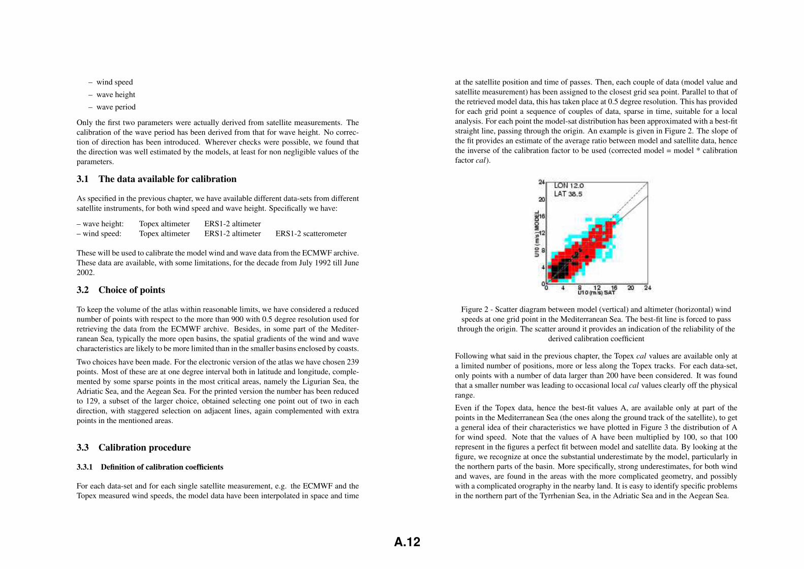
at the satellite position and time of passes. Then, each couple of data (model value andsatellite measurement) has been assigned to the closest grid sea point. Parallel to that ofthe retrieved model data, this has taken place at 0.5 degree resolution. This has providedfor each grid point a sequence of couples of data, sparse in time, suitable for a localanalysis. For each point the model-sat distribution has been approximated with a best-fitstraight line, passing through the origin. An example is given in Figure 2. The slope ofthe fit provides an estimate of the average ratio between model and satellite data, hencethe inverse of the calibration factor to be used (corrected model = model * calibrationfactor cal).

Figure 2 - Scatter diagram between model (vertical) and altimeter (horizontal) windspeeds at one grid point in the Mediterranean Sea. The best-fit line is forced to pass

through the origin. The scatter around it provides an indication of the reliability of thederived calibration coefficient

Following what said in the previous chapter, the Topex cal values are available only ata limited number of positions, more or less along the Topex tracks. For each data-set,only points with a number of data larger than 200 have been considered. It was foundthat a smaller number was leading to occasional local cal values clearly off the physicalrange.

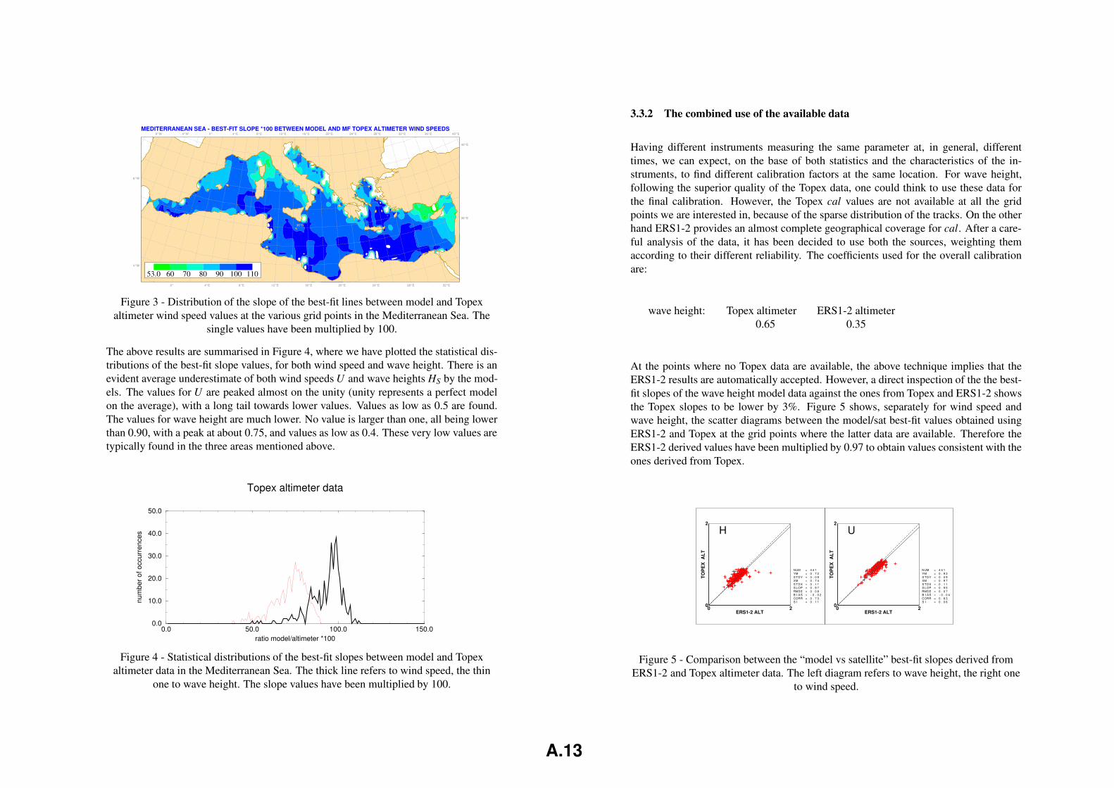
Even if the Topex data, hence the best-fit values A, are available only at part of thepoints in the Mediterranean Sea (the ones along the ground track of the satellite), to geta general idea of their characteristics we have plotted in Figure 3 the distribution of Afor wind speed. Note that the values of A have been multiplied by 100, so that 100represent in the figures a perfect fit between model and satellite data. By looking at thefigure, we recognize at once the substantial underestimate by the model, particularly inthe northern parts of the basin. More specifically, strong underestimates, for both windand waves, are found in the areas with the more complicated geometry, and possiblywith a complicated orography in the nearby land. It is easy to identify specific problemsin the northern part of the Tyrrhenian Sea, in the Adriatic Sea and in the Aegean Sea.

A.12

MEDITERRANEAN SEA - BEST-FIT SLOPE *100 BETWEEN MODEL AND MF TOPEX ALTIMETER WIND SPEEDS

32°N

36°N

40°N

44°N

8°W

8°W

4°W

4°W

0°

0°

4°E

4°E

8°E

8°E

12°E

12°E

16°E

16°E

20°E

20°E

24°E

24°E

28°E

28°E

32°E

32°E 36°E

36°E

40°E

40°E

32°N

36°N

40°N

44°N

8°W

8°W

4°W

4°W

0°

0°

4°E

4°E

8°E

8°E

12°E

12°E

16°E

16°E

20°E

20°E

24°E

24°E

28°E

28°E

32°E

32°E 36°E

36°E

40°E

40°E

53.0 60 70 80 90 100 110

Figure 3 - Distribution of the slope of the best-fit lines between model and Topexaltimeter wind speed values at the various grid points in the Mediterranean Sea. The

single values have been multiplied by 100.

The above results are summarised in Figure 4, where we have plotted the statistical dis-tributions of the best-fit slope values, for both wind speed and wave height. There is anevident average underestimate of both wind speeds U and wave heights HS by the mod-els. The values for U are peaked almost on the unity (unity represents a perfect modelon the average), with a long tail towards lower values. Values as low as 0.5 are found.The values for wave height are much lower. No value is larger than one, all being lowerthan 0.90, with a peak at about 0.75, and values as low as 0.4. These very low values aretypically found in the three areas mentioned above.

0.0 50.0 100.0 150.0ratio model/altimeter *100

0.0

10.0

20.0

30.0

40.0

50.0

num

ber o

f occ

urre

nces

Topex altimeter data

Figure 4 - Statistical distributions of the best-fit slopes between model and Topexaltimeter data in the Mediterranean Sea. The thick line refers to wind speed, the thin

one to wave height. The slope values have been multiplied by 100.

3.3.2 The combined use of the available data

Having different instruments measuring the same parameter at, in general, differenttimes, we can expect, on the base of both statistics and the characteristics of the in-struments, to find different calibration factors at the same location. For wave height,following the superior quality of the Topex data, one could think to use these data forthe final calibration. However, the Topex cal values are not available at all the gridpoints we are interested in, because of the sparse distribution of the tracks. On the otherhand ERS1-2 provides an almost complete geographical coverage for cal. After a care-ful analysis of the data, it has been decided to use both the sources, weighting themaccording to their different reliability. The coefficients used for the overall calibrationare:

wave height: Topex altimeter ERS1-2 altimeter0.65 0.35

At the points where no Topex data are available, the above technique implies that theERS1-2 results are automatically accepted. However, a direct inspection of the the best-fit slopes of the wave height model data against the ones from Topex and ERS1-2 showsthe Topex slopes to be lower by 3%. Figure 5 shows, separately for wind speed andwave height, the scatter diagrams between the model/sat best-fit values obtained usingERS1-2 and Topex at the grid points where the latter data are available. Therefore theERS1-2 derived values have been multiplied by 0.97 to obtain values consistent with theones derived from Topex.

0 2ERS1-2 ALT

0

2

TOP

EX

ALT

H

S I = 0 . 1 1CORR = 0 . 7 3B I A S = - 0 . 0 2RMS E = 0 . 0 8S L OP = 0 . 9 7S T DX = 0 . 1 1XM = 0 . 7 4S T DY = 0 . 0 9YM = 0 . 7 2NUM = 4 4 1

0 2ERS1-2 ALT

0

2

TOP

EX

ALT

U

S I = 0 . 0 6CORR = 0 . 8 3B I A S = - 0 . 0 4RMS E = 0 . 0 7S L OP = 0 . 9 5S T DX = 0 . 1 1XM = 0 . 9 7S T DY = 0 . 0 9YM = 0 . 9 3NUM = 4 4 1

Figure 5 - Comparison between the “model vs satellite” best-fit slopes derived fromERS1-2 and Topex altimeter data. The left diagram refers to wave height, the right one

to wind speed.

A.13

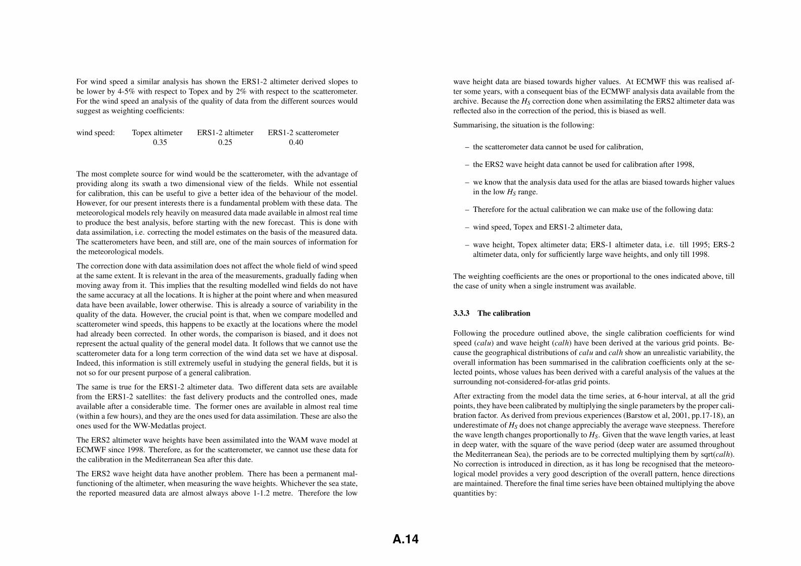
For wind speed a similar analysis has shown the ERS1-2 altimeter derived slopes tobe lower by 4-5% with respect to Topex and by 2% with respect to the scatterometer.For the wind speed an analysis of the quality of data from the different sources wouldsuggest as weighting coefficients:

wind speed: Topex altimeter ERS1-2 altimeter ERS1-2 scatterometer0.35 0.25 0.40

The most complete source for wind would be the scatterometer, with the advantage ofproviding along its swath a two dimensional view of the fields. While not essentialfor calibration, this can be useful to give a better idea of the behaviour of the model.However, for our present interests there is a fundamental problem with these data. Themeteorological models rely heavily on measured data made available in almost real timeto produce the best analysis, before starting with the new forecast. This is done withdata assimilation, i.e. correcting the model estimates on the basis of the measured data.The scatterometers have been, and still are, one of the main sources of information forthe meteorological models.

The correction done with data assimilation does not affect the whole field of wind speedat the same extent. It is relevant in the area of the measurements, gradually fading whenmoving away from it. This implies that the resulting modelled wind fields do not havethe same accuracy at all the locations. It is higher at the point where and when measureddata have been available, lower otherwise. This is already a source of variability in thequality of the data. However, the crucial point is that, when we compare modelled andscatterometer wind speeds, this happens to be exactly at the locations where the modelhad already been corrected. In other words, the comparison is biased, and it does notrepresent the actual quality of the general model data. It follows that we cannot use thescatterometer data for a long term correction of the wind data set we have at disposal.Indeed, this information is still extremely useful in studying the general fields, but it isnot so for our present purpose of a general calibration.

The same is true for the ERS1-2 altimeter data. Two different data sets are availablefrom the ERS1-2 satellites: the fast delivery products and the controlled ones, madeavailable after a considerable time. The former ones are available in almost real time(within a few hours), and they are the ones used for data assimilation. These are also theones used for the WW-Medatlas project.

The ERS2 altimeter wave heights have been assimilated into the WAM wave model atECMWF since 1998. Therefore, as for the scatterometer, we cannot use these data forthe calibration in the Mediterranean Sea after this date.

The ERS2 wave height data have another problem. There has been a permanent mal-functioning of the altimeter, when measuring the wave heights. Whichever the sea state,the reported measured data are almost always above 1-1.2 metre. Therefore the low

wave height data are biased towards higher values. At ECMWF this was realised af-ter some years, with a consequent bias of the ECMWF analysis data available from thearchive. Because the HS correction done when assimilating the ERS2 altimeter data wasreflected also in the correction of the period, this is biased as well.

Summarising, the situation is the following:

– the scatterometer data cannot be used for calibration,

– the ERS2 wave height data cannot be used for calibration after 1998,

– we know that the analysis data used for the atlas are biased towards higher valuesin the low HS range.

– Therefore for the actual calibration we can make use of the following data:

– wind speed, Topex and ERS1-2 altimeter data,

– wave height, Topex altimeter data; ERS-1 altimeter data, i.e. till 1995; ERS-2altimeter data, only for sufficiently large wave heights, and only till 1998.

The weighting coefficients are the ones or proportional to the ones indicated above, tillthe case of unity when a single instrument was available.

3.3.3 The calibration

Following the procedure outlined above, the single calibration coefficients for windspeed (calu) and wave height (calh) have been derived at the various grid points. Be-cause the geographical distributions of calu and calh show an unrealistic variability, theoverall information has been summarised in the calibration coefficients only at the se-lected points, whose values has been derived with a careful analysis of the values at thesurrounding not-considered-for-atlas grid points.

After extracting from the model data the time series, at 6-hour interval, at all the gridpoints, they have been calibrated by multiplying the single parameters by the proper cali-bration factor. As derived from previous experiences (Barstow et al, 2001, pp.17-18), anunderestimate of HS does not change appreciably the average wave steepness. Thereforethe wave length changes proportionally to HS. Given that the wave length varies, at leastin deep water, with the square of the wave period (deep water are assumed throughoutthe Mediterranean Sea), the periods are to be corrected multiplying them by sqrt(calh).No correction is introduced in direction, as it has long be recognised that the meteoro-logical model provides a very good description of the overall pattern, hence directionsare maintained. Therefore the final time series have been obtained multiplying the abovequantities by:

A.14

– HS calh– DirH no correction– TP sqrt(calh)– Tm sqrt(calh)– U calu– DirU no correction

This procedure has been applied separately to the data before and after 20 November2000, i.e. when the substantial change of resolution in the operational ECMWF meteo-rological model implied a change of quality of the wind, hence wave, fields. Thereforefor the first period we have at disposal 101 months of data, and only 19 for the later one.

3.4 Analysis of the calibration procedure

In this section we analyse the accuracy of the calibrated data, wind speed and waveheight, in the Mediterranean Sea.

In a previous chapter we have pointed out that there is a number of random errors in thecalibration. They mainly concern the measurements by the satellites and the capabilityby the models to respond to different situations. These errors lead to the large scatterwe find in the best-fit at each specific location. This is also the reason why we findan unrealistic spatial variability of the calibration coefficients, that forces to summarisethe information only at the selected points. Each selected point represents the summaryof the information available in the surrounding area. This variability is present also inthe open sea, where there is no physical reason for it. It shows the lack of reliabilityof the single estimates of the best-fit slopes. However, the variability increases evenmore when we move close to the coasts, particularly along the northern coasts of theMediterranean Sea. The reason is that the whole European coast is characterised by amarked orography. As most of the storms that affect the Mediterranean Sea come fromthe northern sectors, the marine areas along the northern coasts are on the lee of themountains. We have already mentioned that the altimeter data of wind speed are notaccurate up to the specifications in the first 100 km off the coast. Assimilated in themeteorological model, their error is transmitted also to the wave field.

We can have an idea of the consequent uncertainty of the final estimate of the calibrationcoefficients by considering the scatter index SI of the single best-fits. SI is defined asthe ratio between the root mean square (rms) error σ (model - measured datum) and theaverage value of the interested quantity, either wind speed U or significant wave heightHS. In practice SI provides a non-dimensional estimate of σ. The distributions of theSI values in the Mediterranean Sea, for U and HS, are given in Figure 6 and Figure 7,respectively. This information is an essential complement of the data provided by theatlas, to be presented with all the statistics there included.

MEDITERRANEAN SEA - SCATTER INDEX*100 BETWEEN MODEL (<20001121) AND SATELLITE WIND SPEEDS

32°N

36°N

40°N

44°N

8°W

8°W

4°W

4°W

0°

0°

4°E

4°E

8°E

8°E

12°E

12°E

16°E

16°E

20°E

20°E

24°E

24°E

28°E

28°E

32°E

32°E 36°E

36°E

40°E

40°E

32°N

36°N

40°N

44°N

8°W

8°W

4°W

4°W

0°

0°

4°E

4°E

8°E

8°E

12°E

12°E

16°E

16°E

20°E

20°E

24°E

24°E

28°E

28°E

32°E

32°E 36°E

36°E

40°E

40°E

21 24 28 32 36 40 44 48 50

Figure 6 - Distribution of the scatter index of the best-fit between modelled and satellitemeasured wind speeds. Figures are in percent. The period considered is before 21

November 2000.

We have to consider also the systematic errors. They are hidden, because in general theydo not appear in the best-fit procedure. They do so when the errors have been correctedat a certain date. This is the case with the results of the WAM model in the first 100-200km off the coast. In this range the previous integration scheme was biased towards lowvalues. As already discussed in a previous chapter, this was corrected in the operationalmodel in December 1996. Therefore before this date all the short fetch data have apermanent error towards the low values. Given the directions most of the storms comefrom, this is particularly true along the northern coasts of the Mediterranean Sea.

MEDITERRANEAN SEA - SCATTER INDEX*100 BETWEEN MODEL (<20001121) AND SATELLITE WAVE HEIGHTS

32°N

36°N

40°N

44°N

8°W

8°W

4°W

4°W

0°

0°

4°E

4°E

8°E

8°E

12°E

12°E

16°E

16°E

20°E

20°E

24°E

24°E

28°E

28°E

32°E

32°E 36°E

36°E

40°E

40°E

32°N

36°N

40°N

44°N

8°W

8°W

4°W

4°W

0°

0°

4°E

4°E

8°E

8°E

12°E

12°E

16°E

16°E

20°E

20°E

24°E

24°E

28°E

28°E

32°E

32°E 36°E

36°E

40°E

40°E

26 28 32 36 40 44 48 52 55

Figure 7 - Distribution of the scatter index of the best-fit between modelled and satellitemeasured wave heights. Figures are in percent. The period considered is before 21

November 2000.

A.15

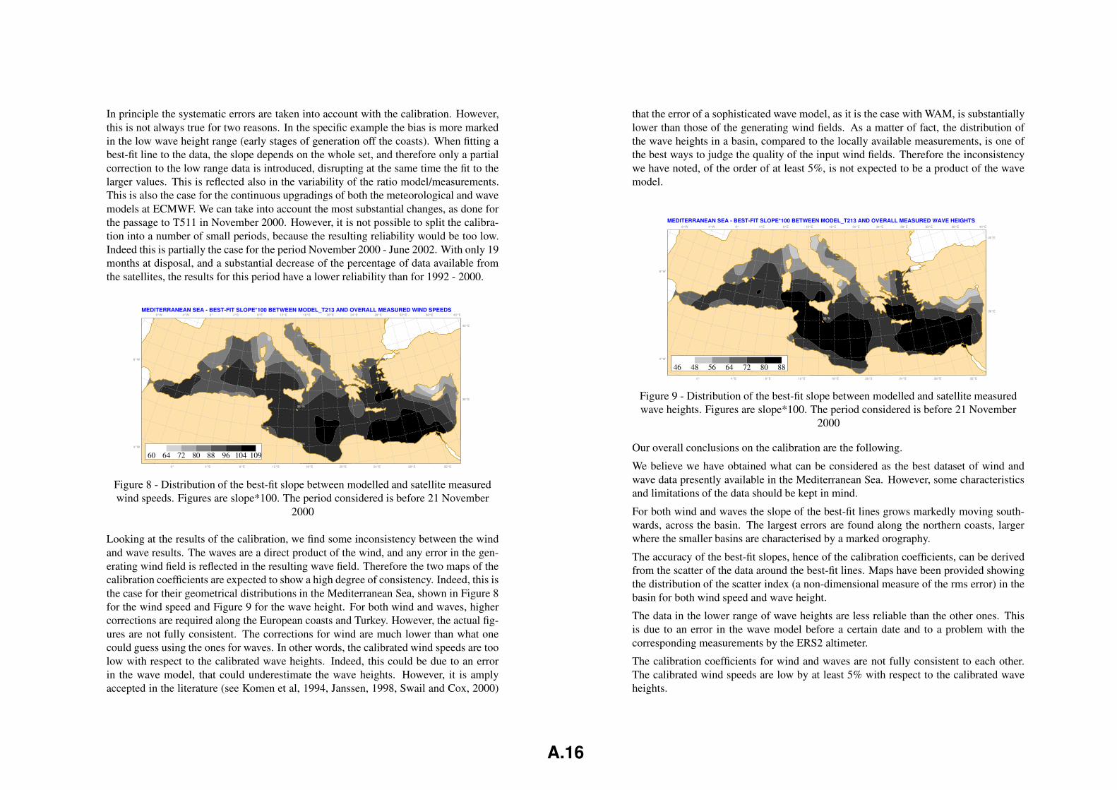
In principle the systematic errors are taken into account with the calibration. However,this is not always true for two reasons. In the specific example the bias is more markedin the low wave height range (early stages of generation off the coasts). When fitting abest-fit line to the data, the slope depends on the whole set, and therefore only a partialcorrection to the low range data is introduced, disrupting at the same time the fit to thelarger values. This is reflected also in the variability of the ratio model/measurements.This is also the case for the continuous upgradings of both the meteorological and wavemodels at ECMWF. We can take into account the most substantial changes, as done forthe passage to T511 in November 2000. However, it is not possible to split the calibra-tion into a number of small periods, because the resulting reliability would be too low.Indeed this is partially the case for the period November 2000 - June 2002. With only 19months at disposal, and a substantial decrease of the percentage of data available fromthe satellites, the results for this period have a lower reliability than for 1992 - 2000.

MEDITERRANEAN SEA - BEST-FIT SLOPE*100 BETWEEN MODEL_T213 AND OVERALL MEASURED WIND SPEEDS

32°N

36°N

40°N

44°N

8°W

8°W

4°W

4°W

0°

0°

4°E

4°E

8°E

8°E

12°E

12°E

16°E

16°E

20°E

20°E

24°E

24°E

28°E

28°E

32°E

32°E 36°E

36°E

40°E

40°E

32°N

36°N

40°N

44°N

8°W

8°W

4°W

4°W

0°

0°

4°E

4°E

8°E

8°E

12°E

12°E

16°E

16°E

20°E

20°E

24°E

24°E

28°E

28°E

32°E

32°E 36°E

36°E

40°E

40°E

60 64 72 80 88 96 104 109

Figure 8 - Distribution of the best-fit slope between modelled and satellite measuredwind speeds. Figures are slope*100. The period considered is before 21 November

2000

Looking at the results of the calibration, we find some inconsistency between the windand wave results. The waves are a direct product of the wind, and any error in the gen-erating wind field is reflected in the resulting wave field. Therefore the two maps of thecalibration coefficients are expected to show a high degree of consistency. Indeed, this isthe case for their geometrical distributions in the Mediterranean Sea, shown in Figure 8for the wind speed and Figure 9 for the wave height. For both wind and waves, highercorrections are required along the European coasts and Turkey. However, the actual fig-ures are not fully consistent. The corrections for wind are much lower than what onecould guess using the ones for waves. In other words, the calibrated wind speeds are toolow with respect to the calibrated wave heights. Indeed, this could be due to an errorin the wave model, that could underestimate the wave heights. However, it is amplyaccepted in the literature (see Komen et al, 1994, Janssen, 1998, Swail and Cox, 2000)

that the error of a sophisticated wave model, as it is the case with WAM, is substantiallylower than those of the generating wind fields. As a matter of fact, the distribution ofthe wave heights in a basin, compared to the locally available measurements, is one ofthe best ways to judge the quality of the input wind fields. Therefore the inconsistencywe have noted, of the order of at least 5%, is not expected to be a product of the wavemodel.

MEDITERRANEAN SEA - BEST-FIT SLOPE*100 BETWEEN MODEL_T213 AND OVERALL MEASURED WAVE HEIGHTS

32°N

36°N

40°N

44°N

8°W

8°W

4°W

4°W

0°

0°

4°E

4°E

8°E

8°E

12°E

12°E

16°E

16°E

20°E

20°E

24°E

24°E

28°E

28°E

32°E

32°E 36°E

36°E

40°E

40°E

32°N

36°N

40°N

44°N

8°W

8°W

4°W

4°W

0°

0°

4°E

4°E

8°E

8°E

12°E

12°E

16°E

16°E

20°E

20°E

24°E

24°E

28°E

28°E

32°E

32°E 36°E

36°E

40°E

40°E

46 48 56 64 72 80 88

Figure 9 - Distribution of the best-fit slope between modelled and satellite measuredwave heights. Figures are slope*100. The period considered is before 21 November

2000

Our overall conclusions on the calibration are the following.

We believe we have obtained what can be considered as the best dataset of wind andwave data presently available in the Mediterranean Sea. However, some characteristicsand limitations of the data should be kept in mind.

For both wind and waves the slope of the best-fit lines grows markedly moving south-wards, across the basin. The largest errors are found along the northern coasts, largerwhere the smaller basins are characterised by a marked orography.

The accuracy of the best-fit slopes, hence of the calibration coefficients, can be derivedfrom the scatter of the data around the best-fit lines. Maps have been provided showingthe distribution of the scatter index (a non-dimensional measure of the rms error) in thebasin for both wind speed and wave height.

The data in the lower range of wave heights are less reliable than the other ones. Thisis due to an error in the wave model before a certain date and to a problem with thecorresponding measurements by the ERS2 altimeter.

The calibration coefficients for wind and waves are not fully consistent to each other.The calibrated wind speeds are low by at least 5% with respect to the calibrated waveheights.

A.16

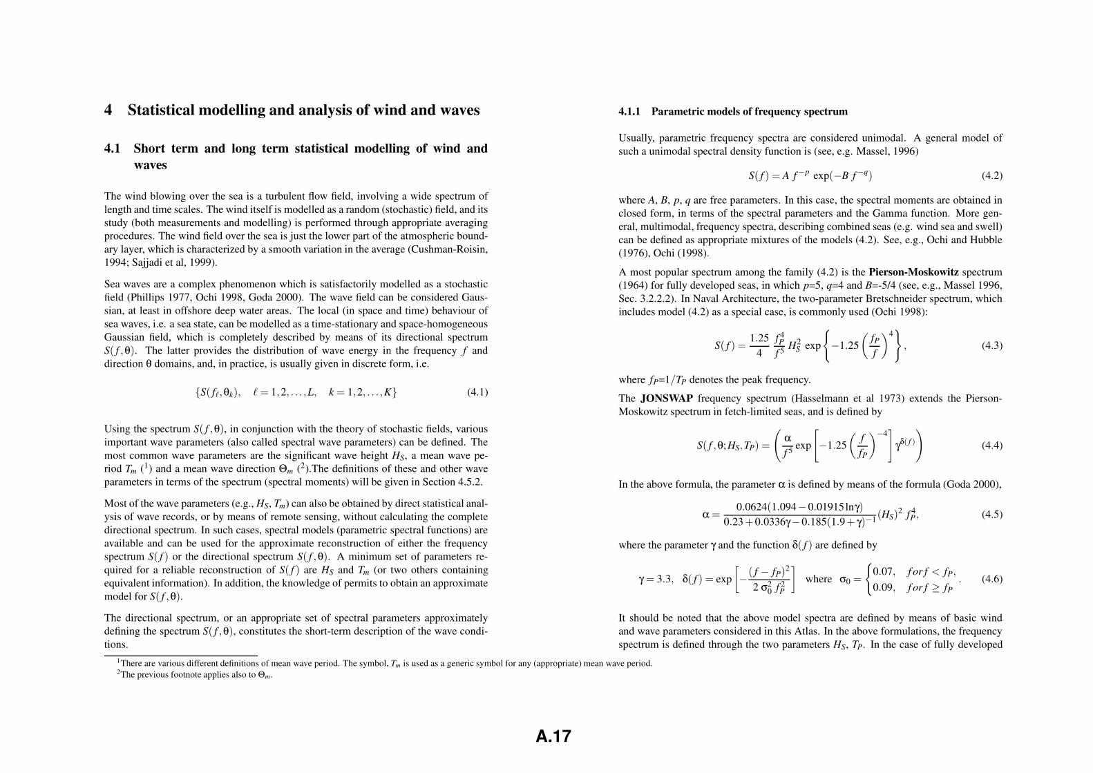
4 Statistical modelling and analysis of wind and waves

4.1 Short term and long term statistical modelling of wind andwaves

The wind blowing over the sea is a turbulent flow field, involving a wide spectrum oflength and time scales. The wind itself is modelled as a random (stochastic) field, and itsstudy (both measurements and modelling) is performed through appropriate averagingprocedures. The wind field over the sea is just the lower part of the atmospheric bound-ary layer, which is characterized by a smooth variation in the average (Cushman-Roisin,1994; Sajjadi et al, 1999).

Sea waves are a complex phenomenon which is satisfactorily modelled as a stochasticfield (Phillips 1977, Ochi 1998, Goda 2000). The wave field can be considered Gaus-sian, at least in offshore deep water areas. The local (in space and time) behaviour ofsea waves, i.e. a sea state, can be modelled as a time-stationary and space-homogeneousGaussian field, which is completely described by means of its directional spectrumS( f ,θ). The latter provides the distribution of wave energy in the frequency f anddirection θ domains, and, in practice, is usually given in discrete form, i.e.

{S( f`,θk), ` = 1,2, . . . ,L, k = 1,2, . . . ,K} (4.1)

Using the spectrum S( f ,θ), in conjunction with the theory of stochastic fields, variousimportant wave parameters (also called spectral wave parameters) can be defined. Themost common wave parameters are the significant wave height HS, a mean wave pe-riod Tm (1) and a mean wave direction Θm (2).The definitions of these and other waveparameters in terms of the spectrum (spectral moments) will be given in Section 4.5.2.

Most of the wave parameters (e.g., HS, Tm) can also be obtained by direct statistical anal-ysis of wave records, or by means of remote sensing, without calculating the completedirectional spectrum. In such cases, spectral models (parametric spectral functions) areavailable and can be used for the approximate reconstruction of either the frequencyspectrum S( f ) or the directional spectrum S( f ,θ). A minimum set of parameters re-quired for a reliable reconstruction of S( f ) are HS and Tm (or two others containingequivalent information). In addition, the knowledge of permits to obtain an approximatemodel for S( f ,θ).

The directional spectrum, or an appropriate set of spectral parameters approximatelydefining the spectrum S( f ,θ), constitutes the short-term description of the wave condi-tions.

4.1.1 Parametric models of frequency spectrum

Usually, parametric frequency spectra are considered unimodal. A general model ofsuch a unimodal spectral density function is (see, e.g. Massel, 1996)

S( f ) = A f−p exp(−B f−q) (4.2)

where A, B, p, q are free parameters. In this case, the spectral moments are obtained inclosed form, in terms of the spectral parameters and the Gamma function. More gen-eral, multimodal, frequency spectra, describing combined seas (e.g. wind sea and swell)can be defined as appropriate mixtures of the models (4.2). See, e.g., Ochi and Hubble(1976), Ochi (1998).

A most popular spectrum among the family (4.2) is the Pierson-Moskowitz spectrum(1964) for fully developed seas, in which p=5, q=4 and B=-5/4 (see, e.g., Massel 1996,Sec. 3.2.2.2). In Naval Architecture, the two-parameter Bretschneider spectrum, whichincludes model (4.2) as a special case, is commonly used (Ochi 1998):

S( f ) =1.25

4f 4P

f 5 H2S exp

{

−1.25(

fP

f

)4}

, (4.3)

where fP=1/TP denotes the peak frequency.

The JONSWAP frequency spectrum (Hasselmann et al 1973) extends the Pierson-Moskowitz spectrum in fetch-limited seas, and is defined by

S( f ,θ;HS,TP) =

(

αf 5 exp

[

−1.25(

ffP

)−4]

γδ( f )

)

(4.4)

In the above formula, the parameter α is defined by means of the formula (Goda 2000),

α =0.0624(1.094−0.01915lnγ)

0.23+0.0336γ−0.185(1.9+ γ)−1(HS)2 f 4

P, (4.5)

where the parameter γ and the function δ( f ) are defined by

γ = 3.3, δ( f ) = exp[

−( f − fP)2

2 σ20 f 2

P

]

where σ0 =

{

0.07, f or f < fP,

0.09, f or f ≥ fP. (4.6)

It should be noted that the above model spectra are defined by means of basic windand wave parameters considered in this Atlas. In the above formulations, the frequencyspectrum is defined through the two parameters HS, TP. In the case of fully developed

1There are various different definitions of mean wave period. The symbol, Tm is used as a generic symbol for any (appropriate) mean wave period.2The previous footnote applies also to Θm.

A.17

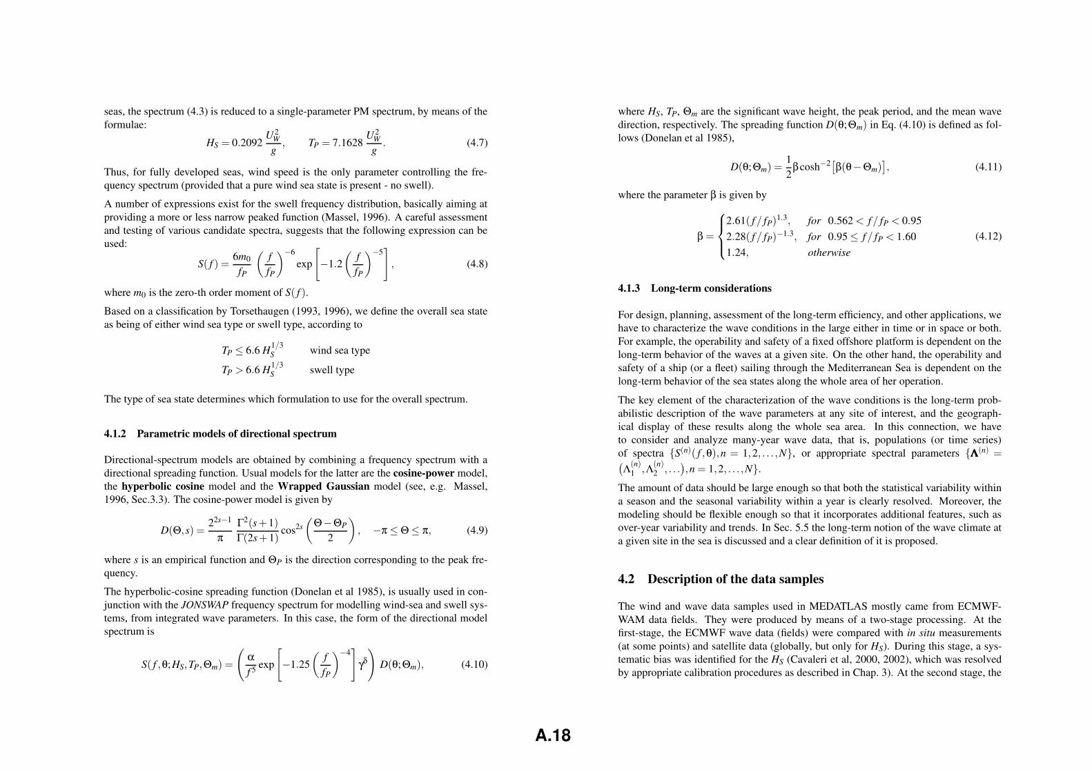
seas, the spectrum (4.3) is reduced to a single-parameter PM spectrum, by means of theformulae:

HS = 0.2092U2

Wg

, TP = 7.1628U2

Wg

. (4.7)

Thus, for fully developed seas, wind speed is the only parameter controlling the fre-quency spectrum (provided that a pure wind sea state is present - no swell).

A number of expressions exist for the swell frequency distribution, basically aiming atproviding a more or less narrow peaked function (Massel, 1996). A careful assessmentand testing of various candidate spectra, suggests that the following expression can beused:

S( f ) =6m0

fP

(

ffP

)−6

exp

[

−1.2(

ffP

)−5]

, (4.8)

where m0 is the zero-th order moment of S( f ).

Based on a classification by Torsethaugen (1993, 1996), we define the overall sea stateas being of either wind sea type or swell type, according to

TP ≤ 6.6 H1/3S wind sea type

TP > 6.6 H1/3S swell type

The type of sea state determines which formulation to use for the overall spectrum.

4.1.2 Parametric models of directional spectrum

Directional-spectrum models are obtained by combining a frequency spectrum with adirectional spreading function. Usual models for the latter are the cosine-power model,the hyperbolic cosine model and the Wrapped Gaussian model (see, e.g. Massel,1996, Sec.3.3). The cosine-power model is given by

D(Θ,s) =22s−1

πΓ2(s+1)

Γ(2s+1)cos2s

(

Θ−ΘP

2

)

, −π ≤ Θ ≤ π, (4.9)

where s is an empirical function and ΘP is the direction corresponding to the peak fre-quency.

The hyperbolic-cosine spreading function (Donelan et al 1985), is usually used in con-junction with the JONSWAP frequency spectrum for modelling wind-sea and swell sys-tems, from integrated wave parameters. In this case, the form of the directional modelspectrum is

S( f ,θ;HS,TP,Θm) =

(

αf 5 exp

[

−1.25(

ffP

)−4]

γδ

)

D(θ;Θm), (4.10)

where HS, TP, Θm are the significant wave height, the peak period, and the mean wavedirection, respectively. The spreading function D(θ;Θm) in Eq. (4.10) is defined as fol-lows (Donelan et al 1985),

D(θ;Θm) =12

βcosh−2[β(θ−Θm)]

, (4.11)

where the parameter β is given by

β =

2.61( f/ fP)1.3, for 0.562 < f/ fP < 0.952.28( f/ fP)−1.3, for 0.95 ≤ f/ fP < 1.601.24, otherwise

(4.12)

4.1.3 Long-term considerations

For design, planning, assessment of the long-term efficiency, and other applications, wehave to characterize the wave conditions in the large either in time or in space or both.For example, the operability and safety of a fixed offshore platform is dependent on thelong-term behavior of the waves at a given site. On the other hand, the operability andsafety of a ship (or a fleet) sailing through the Mediterranean Sea is dependent on thelong-term behavior of the sea states along the whole area of her operation.

The key element of the characterization of the wave conditions is the long-term prob-abilistic description of the wave parameters at any site of interest, and the geograph-ical display of these results along the whole sea area. In this connection, we haveto consider and analyze many-year wave data, that is, populations (or time series)of spectra {S(n)( f ,θ),n = 1,2, . . . ,N}, or appropriate spectral parameters {ΛΛΛ(n) =(

Λ(n)1 ,Λ(n)

2 , . . .)

,n = 1,2, . . . ,N}.

The amount of data should be large enough so that both the statistical variability withina season and the seasonal variability within a year is clearly resolved. Moreover, themodeling should be flexible enough so that it incorporates additional features, such asover-year variability and trends. In Sec. 5.5 the long-term notion of the wave climate ata given site in the sea is discussed and a clear definition of it is proposed.

4.2 Description of the data samples

The wind and wave data samples used in MEDATLAS mostly came from ECMWF-WAM data fields. They were produced by means of a two-stage processing. At thefirst-stage, the ECMWF wave data (fields) were compared with in situ measurements(at some points) and satellite data (globally, but only for HS). During this stage, a sys-tematic bias was identified for the HS (Cavaleri et al, 2000, 2002), which was resolvedby appropriate calibration procedures as described in Chap. 3). At the second stage, the

A.18

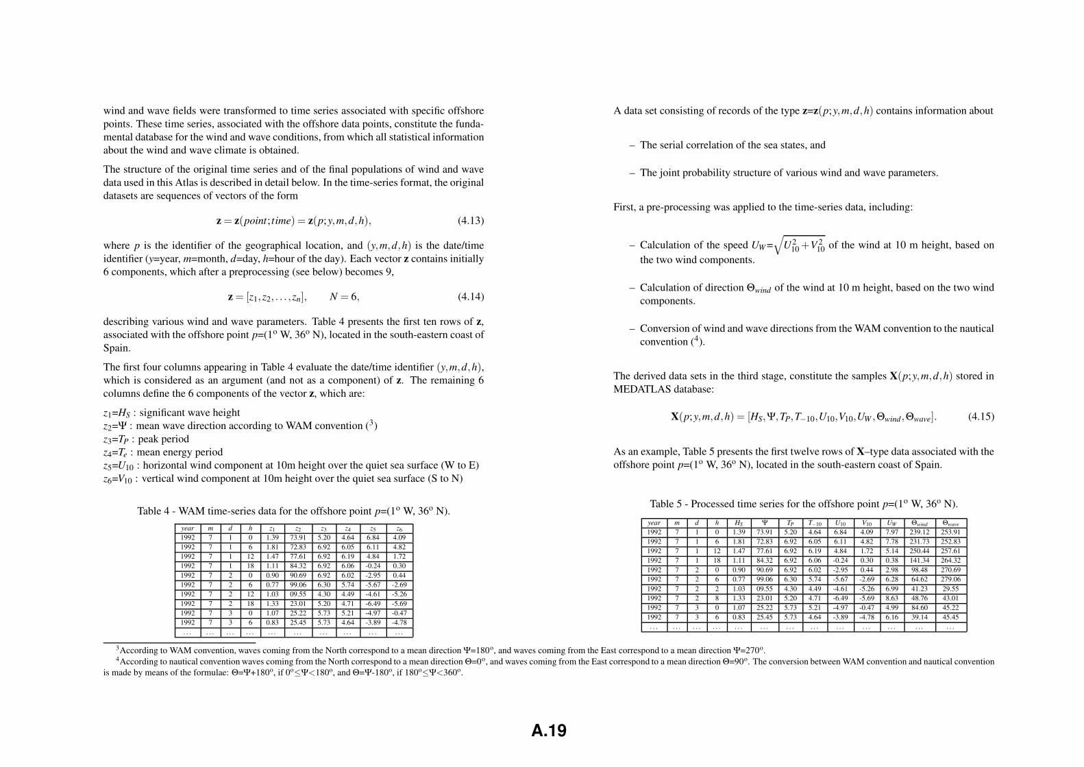
wind and wave fields were transformed to time series associated with specific offshorepoints. These time series, associated with the offshore data points, constitute the funda-mental database for the wind and wave conditions, from which all statistical informationabout the wind and wave climate is obtained.

The structure of the original time series and of the final populations of wind and wavedata used in this Atlas is described in detail below. In the time-series format, the originaldatasets are sequences of vectors of the form

z = z(point; time) = z(p;y,m,d,h), (4.13)

where p is the identifier of the geographical location, and (y,m,d,h) is the date/timeidentifier (y=year, m=month, d=day, h=hour of the day). Each vector z contains initially6 components, which after a preprocessing (see below) becomes 9,

z = [z1,z2, . . . ,zn], N = 6, (4.14)

describing various wind and wave parameters. Table 4 presents the first ten rows of z,associated with the offshore point p=(1o W, 36o N), located in the south-eastern coast ofSpain.

The first four columns appearing in Table 4 evaluate the date/time identifier (y,m,d,h),which is considered as an argument (and not as a component) of z. The remaining 6columns define the 6 components of the vector z, which are:

z1=HS : significant wave heightz2=Ψ : mean wave direction according to WAM convention (3)z3=TP : peak periodz4=Te : mean energy periodz5=U10 : horizontal wind component at 10m height over the quiet sea surface (W to E)z6=V10 : vertical wind component at 10m height over the quiet sea surface (S to N)

Table 4 - WAM time-series data for the offshore point p=(1o W, 36o N).year m d h z1 z2 z3 z4 z5 z61992 7 1 0 1.39 73.91 5.20 4.64 6.84 4.091992 7 1 6 1.81 72.83 6.92 6.05 6.11 4.821992 7 1 12 1.47 77.61 6.92 6.19 4.84 1.721992 7 1 18 1.11 84.32 6.92 6.06 -0.24 0.301992 7 2 0 0.90 90.69 6.92 6.02 -2.95 0.441992 7 2 6 0.77 99.06 6.30 5.74 -5.67 -2.691992 7 2 12 1.03 09.55 4.30 4.49 -4.61 -5.261992 7 2 18 1.33 23.01 5.20 4.71 -6.49 -5.691992 7 3 0 1.07 25.22 5.73 5.21 -4.97 -0.471992 7 3 6 0.83 25.45 5.73 4.64 -3.89 -4.78. . . . . . . . . . . . . . . . . . . . . . . . . . . . . .

A data set consisting of records of the type z=z(p;y,m,d,h) contains information about

– The serial correlation of the sea states, and

– The joint probability structure of various wind and wave parameters.

First, a pre-processing was applied to the time-series data, including:

– Calculation of the speed UW =√

U210 +V 2

10 of the wind at 10 m height, based onthe two wind components.

– Calculation of direction Θwind of the wind at 10 m height, based on the two windcomponents.

– Conversion of wind and wave directions from the WAM convention to the nauticalconvention (4).

The derived data sets in the third stage, constitute the samples X(p;y,m,d,h) stored inMEDATLAS database:

X(p;y,m,d,h) = [HS,Ψ,TP,T−10,U10,V10,UW ,Θwind,Θwave]. (4.15)

As an example, Table 5 presents the first twelve rows of X–type data associated with theoffshore point p=(1o W, 36o N), located in the south-eastern coast of Spain.

Table 5 - Processed time series for the offshore point p=(1o W, 36o N).

year m d h HS Ψ TP T−10 U10 V10 UW Θwind Θwave

1992 7 1 0 1.39 73.91 5.20 4.64 6.84 4.09 7.97 239.12 253.911992 7 1 6 1.81 72.83 6.92 6.05 6.11 4.82 7.78 231.73 252.831992 7 1 12 1.47 77.61 6.92 6.19 4.84 1.72 5.14 250.44 257.611992 7 1 18 1.11 84.32 6.92 6.06 -0.24 0.30 0.38 141.34 264.321992 7 2 0 0.90 90.69 6.92 6.02 -2.95 0.44 2.98 98.48 270.691992 7 2 6 0.77 99.06 6.30 5.74 -5.67 -2.69 6.28 64.62 279.061992 7 2 2 1.03 09.55 4.30 4.49 -4.61 -5.26 6.99 41.23 29.551992 7 2 8 1.33 23.01 5.20 4.71 -6.49 -5.69 8.63 48.76 43.011992 7 3 0 1.07 25.22 5.73 5.21 -4.97 -0.47 4.99 84.60 45.221992 7 3 6 0.83 25.45 5.73 4.64 -3.89 -4.78 6.16 39.14 45.45. . . . . . . . . . . . . . . . . . . . . . . . . . . . . . . . . . . . . . .

3According to WAM convention, waves coming from the North correspond to a mean direction Ψ=180o, and waves coming from the East correspond to a mean direction Ψ=270o.4According to nautical convention waves coming from the North correspond to a mean direction Θ=0o, and waves coming from the East correspond to a mean direction Θ=90o. The conversion between WAM convention and nautical convention

is made by means of the formulae: Θ=Ψ+180o, if 0o≤Ψ<180o, and Θ=Ψ-180o, if 180o≤Ψ<360o.

A.19

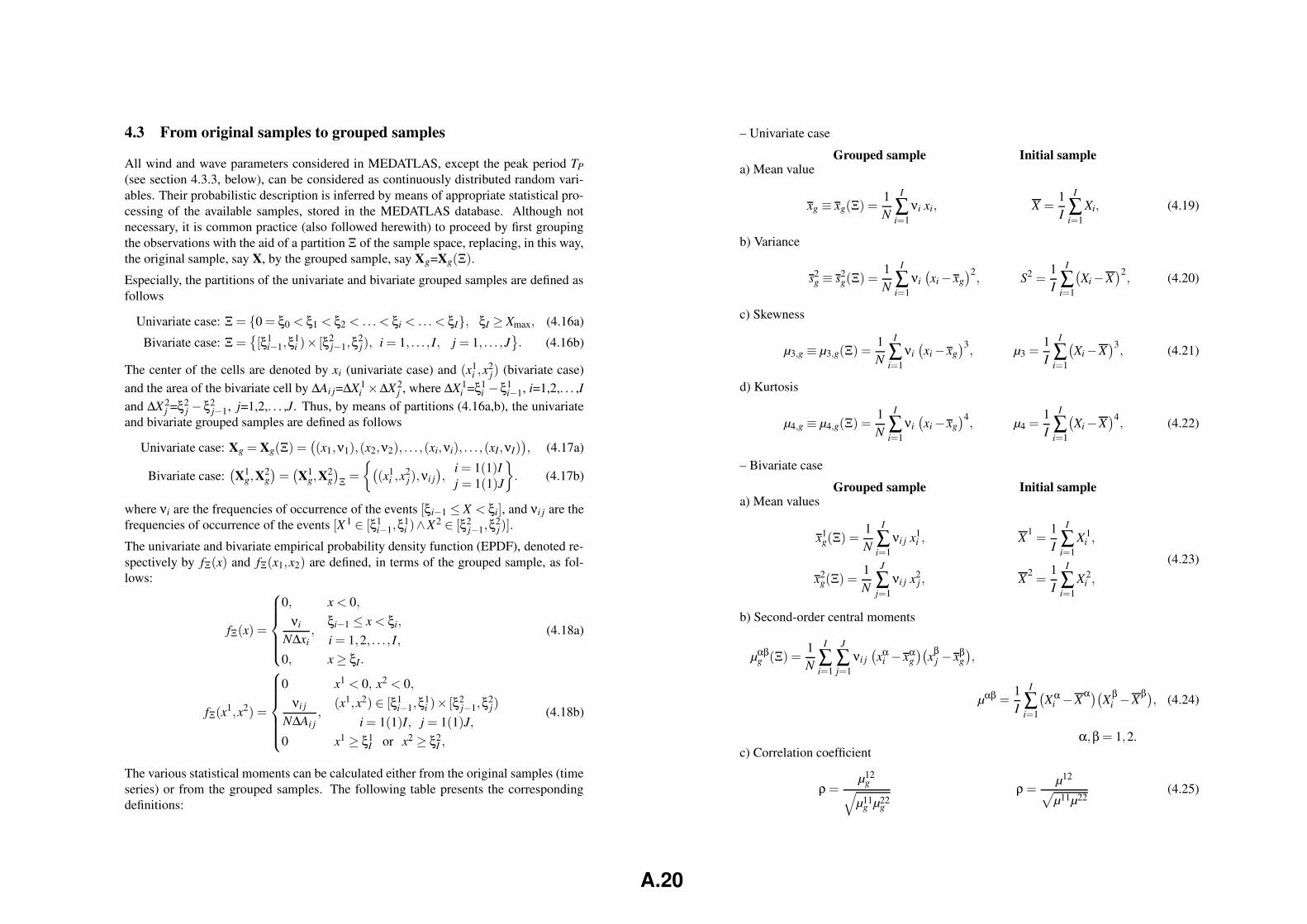
4.3 From original samples to grouped samples

All wind and wave parameters considered in MEDATLAS, except the peak period TP(see section 4.3.3, below), can be considered as continuously distributed random vari-ables. Their probabilistic description is inferred by means of appropriate statistical pro-cessing of the available samples, stored in the MEDATLAS database. Although notnecessary, it is common practice (also followed herewith) to proceed by first groupingthe observations with the aid of a partition Ξ of the sample space, replacing, in this way,the original sample, say X, by the grouped sample, say Xg=Xg(Ξ).

Especially, the partitions of the univariate and bivariate grouped samples are defined asfollows

Univariate case: Ξ = {0 = ξ0 < ξ1 < ξ2 < .. . < ξi < .. . < ξI}, ξI ≥ Xmax, (4.16a)

Bivariate case: Ξ ={

[ξ1i−1,ξ

1i )× [ξ2

j−1,ξ2j), i = 1, . . . , I, j = 1, . . . ,J

}

. (4.16b)

The center of the cells are denoted by xi (univariate case) and (x1i ,x

2j) (bivariate case)

and the area of the bivariate cell by ∆Ai j=∆X1i ×∆X2

j , where ∆X1i =ξ1

i −ξ1i−1, i=1,2,. . . ,I

and ∆X2j =ξ2

j − ξ2j−1, j=1,2,. . . ,J. Thus, by means of partitions (4.16a,b), the univariate

and bivariate grouped samples are defined as follows

Univariate case: Xg = Xg(Ξ) =(

(x1,ν1),(x2,ν2), . . . ,(xi,νi), . . . ,(xI,νI))

, (4.17a)

Bivariate case:(

X1g,X

2g)

=(

X1g,X

2g)

Ξ =

{

(

(x1i ,x

2j),νi j

)

,i = 1(1)Ij = 1(1)J

}

. (4.17b)

where νi are the frequencies of occurrence of the events [ξi−1 ≤ X < ξi], and νi j are thefrequencies of occurrence of the events [X 1 ∈ [ξ1

i−1,ξ1i )∧X2 ∈ [ξ2

j−1,ξ2j)].

The univariate and bivariate empirical probability density function (EPDF), denoted re-spectively by fΞ(x) and fΞ(x1,x2) are defined, in terms of the grouped sample, as fol-lows:

fΞ(x) =

0, x < 0,

νi

N∆xi,

ξi−1 ≤ x < ξi,

i = 1,2, . . . , I,0, x ≥ ξI.

(4.18a)

fΞ(x1,x2) =

0 x1 < 0, x2 < 0,

νi j

N∆Ai j,

(x1,x2) ∈ [ξ1i−1,ξ

1i )× [ξ2

j−1,ξ2j)

i = 1(1)I, j = 1(1)J,0 x1 ≥ ξ1

I or x2 ≥ ξ2I ,

(4.18b)

The various statistical moments can be calculated either from the original samples (timeseries) or from the grouped samples. The following table presents the correspondingdefinitions:

– Univariate case

Grouped sample Initial samplea) Mean value

xg ≡ xg(Ξ) =1N

I

∑i=1

νi xi, X =1I

I

∑i=1

Xi, (4.19)

b) Variance

s2g ≡ s2

g(Ξ) =1N

I

∑i=1

νi(

xi − xg)2

, S2 =1I

I

∑i=1

(

Xi−X)2

, (4.20)

c) Skewness

µ3,g ≡ µ3,g(Ξ) =1N

I

∑i=1

νi(

xi − xg)3

, µ3 =1I

I

∑i=1

(

Xi−X)3

, (4.21)

d) Kurtosis

µ4,g ≡ µ4,g(Ξ) =1N

I

∑i=1

νi(

xi − xg)4

, µ4 =1I

I

∑i=1

(

Xi−X)4

, (4.22)

– Bivariate case

Grouped sample Initial samplea) Mean values

x1g(Ξ) =

1N

I

∑i=1

νi j x1i , X1

=1I

I

∑i=1

X1i ,

x2g(Ξ) =

1N

J

∑j=1

νi j x2j , X2

=1I

I

∑i=1

X2i ,

(4.23)

b) Second-order central moments

µαβg (Ξ) =

1N

I

∑i=1

J

∑j=1

νi j(

xαi − xα

g)(

xβj − xβ

g)

,

µαβ =1I

I

∑i=1

(

Xαi −Xα)(Xβ

i −Xβ), (4.24)

α,β = 1,2.c) Correlation coefficient

ρ =µ12

g√

µ11g µ22

g

ρ =µ12

√

µ11µ22(4.25)

A.20

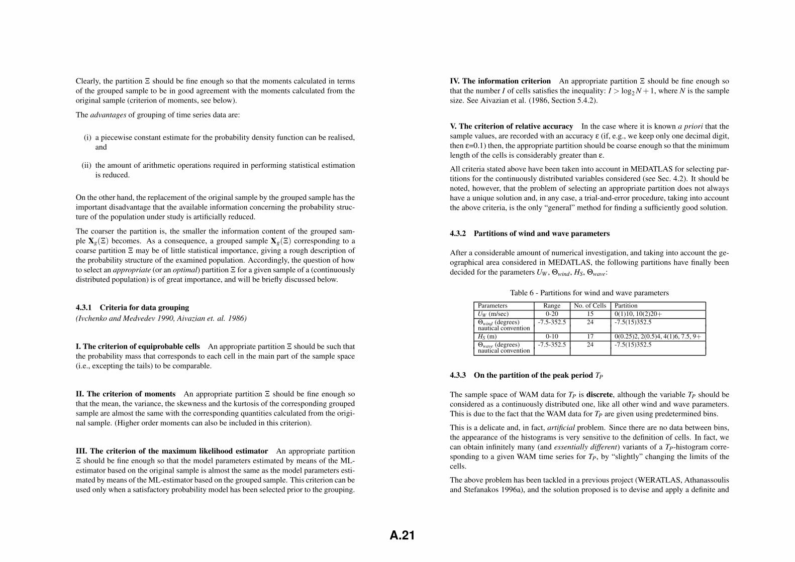
Clearly, the partition Ξ should be fine enough so that the moments calculated in termsof the grouped sample to be in good agreement with the moments calculated from theoriginal sample (criterion of moments, see below).

The advantages of grouping of time series data are:

(i) a piecewise constant estimate for the probability density function can be realised,and

(ii) the amount of arithmetic operations required in performing statistical estimationis reduced.

On the other hand, the replacement of the original sample by the grouped sample has theimportant disadvantage that the available information concerning the probability struc-ture of the population under study is artificially reduced.

The coarser the partition is, the smaller the information content of the grouped sam-ple Xg(Ξ) becomes. As a consequence, a grouped sample Xg(Ξ) corresponding to acoarse partition Ξ may be of little statistical importance, giving a rough description ofthe probability structure of the examined population. Accordingly, the question of howto select an appropriate (or an optimal) partition Ξ for a given sample of a (continuouslydistributed population) is of great importance, and will be briefly discussed below.

4.3.1 Criteria for data grouping(Ivchenko and Medvedev 1990, Aivazian et. al. 1986)

I. The criterion of equiprobable cells An appropriate partition Ξ should be such thatthe probability mass that corresponds to each cell in the main part of the sample space(i.e., excepting the tails) to be comparable.

II. The criterion of moments An appropriate partition Ξ should be fine enough sothat the mean, the variance, the skewness and the kurtosis of the corresponding groupedsample are almost the same with the corresponding quantities calculated from the origi-nal sample. (Higher order moments can also be included in this criterion).

III. The criterion of the maximum likelihood estimator An appropriate partitionΞ should be fine enough so that the model parameters estimated by means of the ML-estimator based on the original sample is almost the same as the model parameters esti-mated by means of the ML-estimator based on the grouped sample. This criterion can beused only when a satisfactory probability model has been selected prior to the grouping.

IV. The information criterion An appropriate partition Ξ should be fine enough sothat the number I of cells satisfies the inequality: I > log2 N +1, where N is the samplesize. See Aivazian et al. (1986, Section 5.4.2).

V. The criterion of relative accuracy In the case where it is known a priori that thesample values, are recorded with an accuracy ε (if, e.g., we keep only one decimal digit,then ε=0.1) then, the appropriate partition should be coarse enough so that the minimumlength of the cells is considerably greater than ε.

All criteria stated above have been taken into account in MEDATLAS for selecting par-titions for the continuously distributed variables considered (see Sec. 4.2). It should benoted, however, that the problem of selecting an appropriate partition does not alwayshave a unique solution and, in any case, a trial-and-error procedure, taking into accountthe above criteria, is the only “general” method for finding a sufficiently good solution.

4.3.2 Partitions of wind and wave parameters

After a considerable amount of numerical investigation, and taking into account the ge-ographical area considered in MEDATLAS, the following partitions have finally beendecided for the parameters UW , Θwind , HS, Θwave:

Table 6 - Partitions for wind and wave parameters

Parameters Range No. of Cells PartitionUW (m/sec) 0-20 15 0(1)10, 10(2)20+Θwind (degrees) -7.5-352.5 24 -7.5(15)352.5nautical conventionHS (m) 0-10 17 0(0.25)2, 2(0.5)4, 4(1)6, 7.5, 9+Θwave (degrees) -7.5-352.5 24 -7.5(15)352.5nautical convention

4.3.3 On the partition of the peak period TP

The sample space of WAM data for TP is discrete, although the variable TP should beconsidered as a continuously distributed one, like all other wind and wave parameters.This is due to the fact that the WAM data for TP are given using predetermined bins.

This is a delicate and, in fact, artificial problem. Since there are no data between bins,the appearance of the histograms is very sensitive to the definition of cells. In fact, wecan obtain infinitely many (and essentially different) variants of a TP-histogram corre-sponding to a given WAM time series for TP, by “slightly” changing the limits of thecells.

The above problem has been tackled in a previous project (WERATLAS, Athanassoulisand Stefanakos 1996a), and the solution proposed is to devise and apply a definite and

A.21

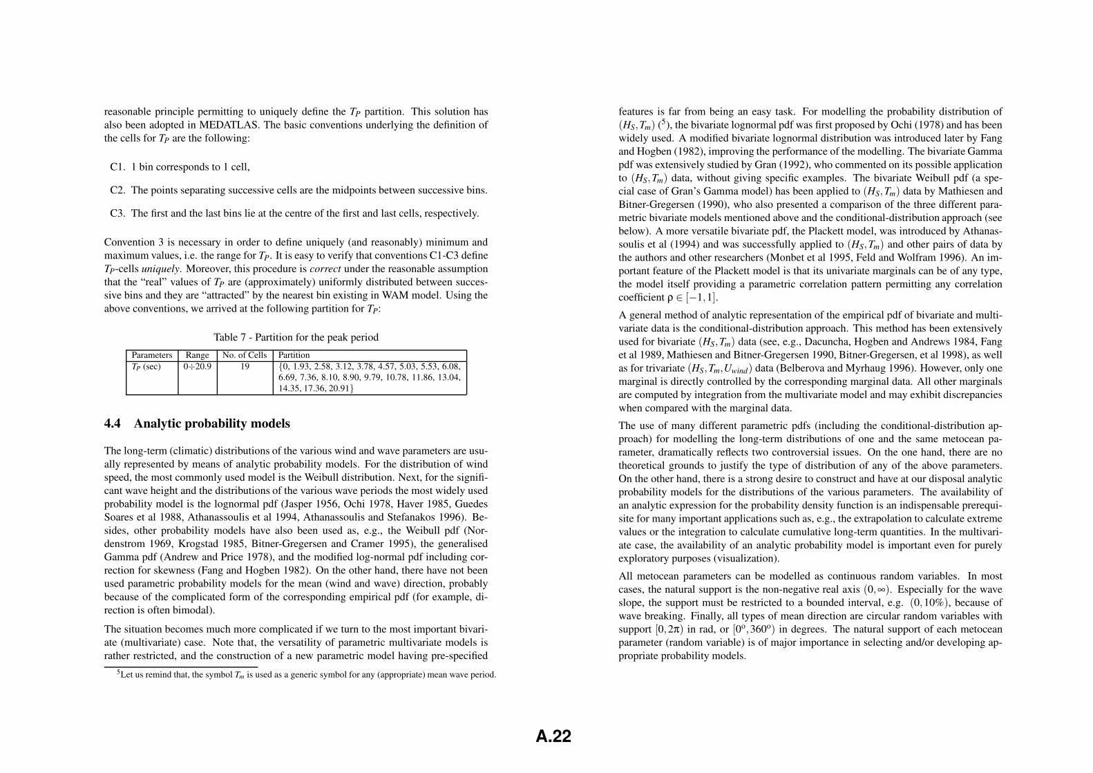
reasonable principle permitting to uniquely define the TP partition. This solution hasalso been adopted in MEDATLAS. The basic conventions underlying the definition ofthe cells for TP are the following:

C1. 1 bin corresponds to 1 cell,

C2. The points separating successive cells are the midpoints between successive bins.

C3. The first and the last bins lie at the centre of the first and last cells, respectively.

Convention 3 is necessary in order to define uniquely (and reasonably) minimum andmaximum values, i.e. the range for TP. It is easy to verify that conventions C1-C3 defineTP-cells uniquely. Moreover, this procedure is correct under the reasonable assumptionthat the “real” values of TP are (approximately) uniformly distributed between succes-sive bins and they are “attracted” by the nearest bin existing in WAM model. Using theabove conventions, we arrived at the following partition for TP:

Table 7 - Partition for the peak period

Parameters Range No. of Cells PartitionTP (sec) 0÷20.9 19 {0, 1.93, 2.58, 3.12, 3.78, 4.57, 5.03, 5.53, 6.08,

6.69, 7.36, 8.10, 8.90, 9.79, 10.78, 11.86, 13.04,14.35, 17.36, 20.91}

4.4 Analytic probability models

The long-term (climatic) distributions of the various wind and wave parameters are usu-ally represented by means of analytic probability models. For the distribution of windspeed, the most commonly used model is the Weibull distribution. Next, for the signifi-cant wave height and the distributions of the various wave periods the most widely usedprobability model is the lognormal pdf (Jasper 1956, Ochi 1978, Haver 1985, GuedesSoares et al 1988, Athanassoulis et al 1994, Athanassoulis and Stefanakos 1996). Be-sides, other probability models have also been used as, e.g., the Weibull pdf (Nor-denstrom 1969, Krogstad 1985, Bitner-Gregersen and Cramer 1995), the generalisedGamma pdf (Andrew and Price 1978), and the modified log-normal pdf including cor-rection for skewness (Fang and Hogben 1982). On the other hand, there have not beenused parametric probability models for the mean (wind and wave) direction, probablybecause of the complicated form of the corresponding empirical pdf (for example, di-rection is often bimodal).

The situation becomes much more complicated if we turn to the most important bivari-ate (multivariate) case. Note that, the versatility of parametric multivariate models israther restricted, and the construction of a new parametric model having pre-specified

features is far from being an easy task. For modelling the probability distribution of(HS,Tm) (5), the bivariate lognormal pdf was first proposed by Ochi (1978) and has beenwidely used. A modified bivariate lognormal distribution was introduced later by Fangand Hogben (1982), improving the performance of the modelling. The bivariate Gammapdf was extensively studied by Gran (1992), who commented on its possible applicationto (HS,Tm) data, without giving specific examples. The bivariate Weibull pdf (a spe-cial case of Gran’s Gamma model) has been applied to (HS,Tm) data by Mathiesen andBitner-Gregersen (1990), who also presented a comparison of the three different para-metric bivariate models mentioned above and the conditional-distribution approach (seebelow). A more versatile bivariate pdf, the Plackett model, was introduced by Athanas-soulis et al (1994) and was successfully applied to (HS,Tm) and other pairs of data bythe authors and other researchers (Monbet et al 1995, Feld and Wolfram 1996). An im-portant feature of the Plackett model is that its univariate marginals can be of any type,the model itself providing a parametric correlation pattern permitting any correlationcoefficient ρ ∈ [−1,1].

A general method of analytic representation of the empirical pdf of bivariate and multi-variate data is the conditional-distribution approach. This method has been extensivelyused for bivariate (HS,Tm) data (see, e.g., Dacuncha, Hogben and Andrews 1984, Fanget al 1989, Mathiesen and Bitner-Gregersen 1990, Bitner-Gregersen, et al 1998), as wellas for trivariate (HS,Tm,Uwind) data (Belberova and Myrhaug 1996). However, only onemarginal is directly controlled by the corresponding marginal data. All other marginalsare computed by integration from the multivariate model and may exhibit discrepancieswhen compared with the marginal data.

The use of many different parametric pdfs (including the conditional-distribution ap-proach) for modelling the long-term distributions of one and the same metocean pa-rameter, dramatically reflects two controversial issues. On the one hand, there are notheoretical grounds to justify the type of distribution of any of the above parameters.On the other hand, there is a strong desire to construct and have at our disposal analyticprobability models for the distributions of the various parameters. The availability ofan analytic expression for the probability density function is an indispensable prerequi-site for many important applications such as, e.g., the extrapolation to calculate extremevalues or the integration to calculate cumulative long-term quantities. In the multivari-ate case, the availability of an analytic probability model is important even for purelyexploratory purposes (visualization).

All metocean parameters can be modelled as continuous random variables. In mostcases, the natural support is the non-negative real axis (0,∞). Especially for the waveslope, the support must be restricted to a bounded interval, e.g. (0,10%), because ofwave breaking. Finally, all types of mean direction are circular random variables withsupport [0,2π) in rad, or [0o,360o) in degrees. The natural support of each metoceanparameter (random variable) is of major importance in selecting and/or developing ap-propriate probability models.

5Let us remind that, the symbol Tm is used as a generic symbol for any (appropriate) mean wave period.

A.22

An efficient general method for analytic representation of any wind or wave parame-ter (or any combination of them) is the Kernel Density Model (KDM) representation,which has been developed and assessed by Athanassoulis and Belibassakis (2002). Inthis work, a modification of the classical kernel density estimation method has been in-troduced that can serve the purpose of both estimation and analytic representation ofany metocean parameter (the univariate case) or any set of metocean parameters (themultivariate case), provided that a representative histogram is available.

The kernel density model has been first introduced in the context of nonparametric dis-criminant analysis by Fix and Hodges (1951) and has become a central topic in thecontext of nonparametric statistical estimation and regression since the 1970’s; see, e.g.,the informative books by Silverman (1986) and Scott (1995).

In the case of a grouped sample, the kernel density model is (Athanassoulis and Belibas-sakis 2002)

f (x) =1N

I

∑i=1

νi K(x;xi,h), (4.26)

where νi is the relative frequency of the bin xi (i.e., the cell [ξi−1,ξi)), and K(x;xi,h)are smooth, non-negative functions, usually taken to be probability density functions inthemselves, and h is a parameter controlling the bandwidth (essential support) of eachK(x;xi,h). The functions K(x;xi,h) are called kernels and their specific form does notseriously affect the representation, except in the vicinity of the boundary points of thesupport of f (x).

The fixed-bandwidth kernel representation has been found susceptible to local over-smoothing behaviour in the areas of high pdf values, and local undersmoothing be-haviour in areas of low pdf values, especially in the tails of the represented pdf. Instead,the variable-bandwidth kernel representation of the form

f (x) =1N

I

∑i=1

νi K(x;xi,hi), (4.27)

has been chosen. The local bandwidths hi are associated one-to-one with the bins xi.

The kernel density model can be extended in a straightforward way to the multivariatecase; see, e.g., Silverman(1986), Hardle (1991), Wand and Jones (1995). Especially, inthe bivariate case, given the grouped sample

{

(x1i ,x

2j),νi j

}

i=1,(1),I, j=1(1),J , the variable-bandwidth kernel representation is defined by

f (x1,x2) =1N

I

∑i=1

J

∑j=1

νi j K(

x1,x2;(x1i ,x

2j),hi j

)

, (4.28)

If the elements of the bandwidth matrix are assumed to be pairwise independent anduniform along x1 and x2, a multiplicative kernel can be used

K(

x1,x2;(x1i ,x

2j),hi j

)

= K1(

x1;x1i ,h

1i)

K2(

x2;x2j ,h

2j)

(4.29)

which is marginally consistent. Thus, the estimation of the bandwidths hdid can be based

on the marginal data alone.

Taking into account the different support of the various variables considered, new fam-ilies of skewed (asymmetric) kernel functions are developed, suitable for the represen-tation of the pdf’s of linear random variables with support on (0,∞) or (0,s), and ofdirectional (circular) random variables with support on [0o,360o). The kernel functionsconsidered are the univariate Gamma, Lognormal, Beta and Wrapped Gaussian kernels.Special attention has also been paid to the construction of bivariate kernels as tensorproducts of the univariate ones, which are able to represent any bivariate (and, in gen-eral, multivariate) empirical pdf, perfectly conforming with all marginals.

MATLAB codes are available upon request.

4.5 Wind and wave climate in the Mediterranean Sea

The wind and wave climate at a specific site in the sea can be defined by means of thelong-term statistics of the (most) important wind and wave parameters. Traditionally, thetime-series structure of wind and wave parameters is ignored and the latter are treated,in the long-term sense, as random variables. However, the seasonal inhomogeneity isimportant for most applications and should be taken into account. A way to do this is bysubdividing the whole population into classes, according to the season (or month); thisis a common practice in Wind and Wave Atlases; see, e.g., the ones developed by NavalOceanography Command Detachment (1983), Hogben et al (1986), Direccion Generalde Puertos y Costas (1988), Athanassoulis and Skarsoulis (1992). See, also Hogben(1990). Accordingly, the wind and wave climate at a given site in the sea is defined bymeans of the seasonal statistics of the important wind and wave parameters. A morecomplete definition is

The wind and wave climate of a given site in the sea is defined by the setof the joint probability distributions of all important wind and wave param-eters, including at least

i) The bivariate probability distributions:

P(UW ,Θwind|site,season),P(HS,TP|site,season), P(HS,Θwave|site,season),P(HS,UW |site,season),

from which one can also derive:

ii) The corresponding univariate probability distributions:

P(UW |site,season), P(Θwind|site,season),P(HS|site,season), P(TP|site,season), P(Θwave|site,season),

A.23

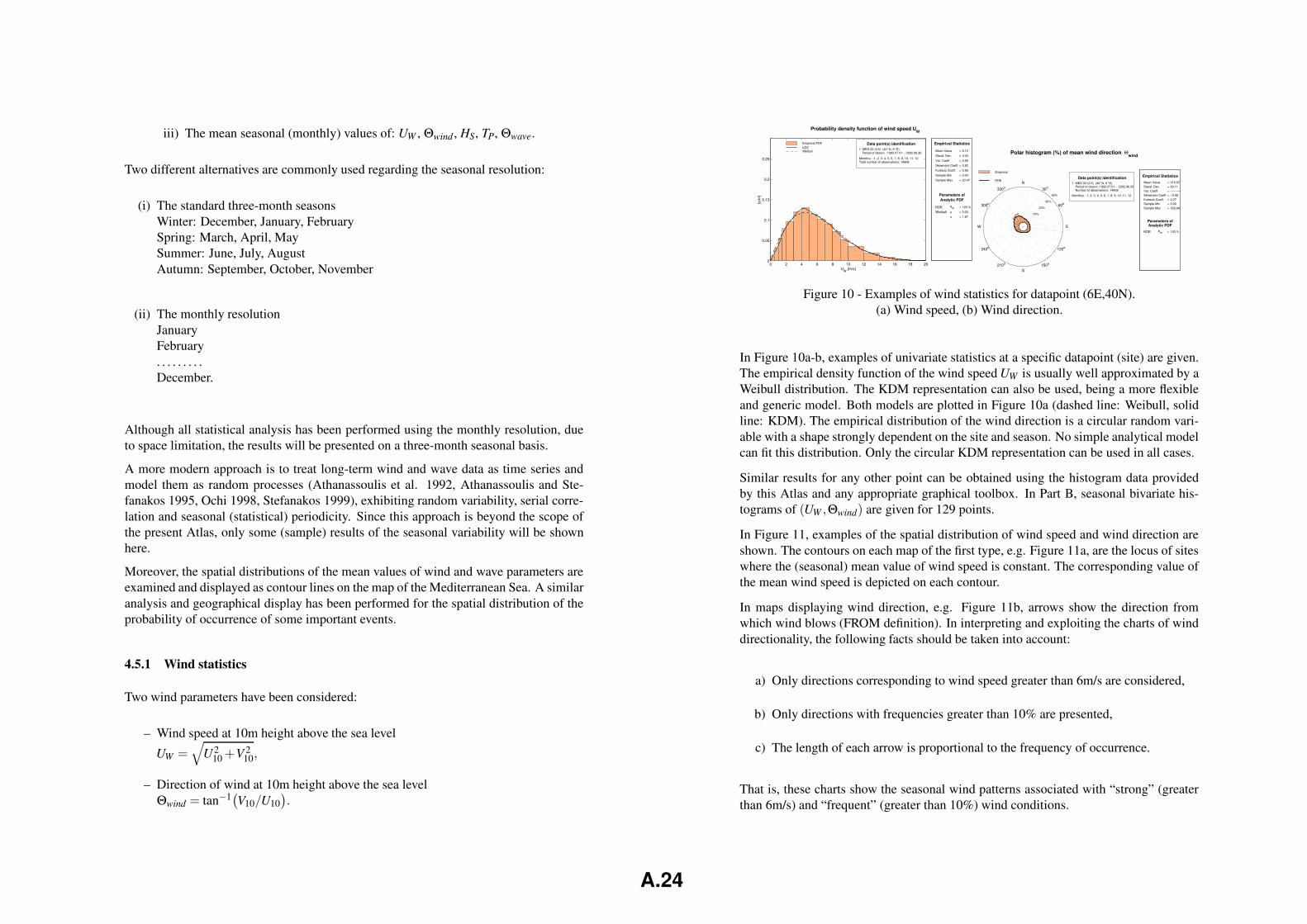
iii) The mean seasonal (monthly) values of: UW , Θwind , HS, TP, Θwave.

Two different alternatives are commonly used regarding the seasonal resolution:

(i) The standard three-month seasonsWinter: December, January, FebruarySpring: March, April, MaySummer: June, July, AugustAutumn: September, October, November

(ii) The monthly resolutionJanuaryFebruary. . . . . . . . .December.

Although all statistical analysis has been performed using the monthly resolution, dueto space limitation, the results will be presented on a three-month seasonal basis.

A more modern approach is to treat long-term wind and wave data as time series andmodel them as random processes (Athanassoulis et al. 1992, Athanassoulis and Ste-fanakos 1995, Ochi 1998, Stefanakos 1999), exhibiting random variability, serial corre-lation and seasonal (statistical) periodicity. Since this approach is beyond the scope ofthe present Atlas, only some (sample) results of the seasonal variability will be shownhere.

Moreover, the spatial distributions of the mean values of wind and wave parameters areexamined and displayed as contour lines on the map of the Mediterranean Sea. A similaranalysis and geographical display has been performed for the spatial distribution of theprobability of occurrence of some important events.

4.5.1 Wind statistics

Two wind parameters have been considered:

– Wind speed at 10m height above the sea level

UW =√

U210 +V 2

10,

– Direction of wind at 10m height above the sea levelΘwind = tan−1(V10/U10

)

.

Probability density function of wind speed UW

Empirical Statistics

Mean Value

Stand. Dev.

Var. Coeff.

Skewness Coeff.

Kurtosis Coeff.

Sample Min

Sample Max

Parameters ofAnalytic PDF

KDE bW

Weibull µσ

=

=

=

=

=

=

=

=

=

=

6.12

3.42

0.56

0.82

0.59

0.03

23.47

120 %

0.03

1.87

0 2 4 6 8 10 12 14 16 18 200

0.05

0.1

0.15

0.2

0.25

UW

[m/s]

[s/m

]

Empirical PDF Data point(s) identification1. MED.33 (0.5) (40°N, 6°E)

Period of observ. :1992.07.01 − 2002.06.30

Month(s) : 1, 2, 3, 4, 5, 6, 7, 8, 9, 10, 11, 12Total number of observations: 14608

KDEWeibull Polar histogram (%) of mean wind direction Θ

wind

Empirical Statistics

Mean ValueStand. Dev.Var. Coeff.Skewness Coeff.Kurtosis Coeff.Sample MinSample Max

Parameters ofAnalytic PDF

KDE bW

=======

=

319.9790.11−−−−−−−0.080.370.00359.94

120 %

N

30o

60o

E

120o

150o

S210o

240o

W

300o

330o

10%

20%

30%

40%

Empirical

Data point(s) identification1. MED.33 (0.5) (40°N, 6°E) Period of observ.:1992.07.01 − 2002.06.30 Number of observations: 14608

Month(s) : 1, 2, 3, 4, 5, 6, 7, 8, 9, 10, 11, 12

KDE

Figure 10 - Examples of wind statistics for datapoint (6E,40N).(a) Wind speed, (b) Wind direction.

In Figure 10a-b, examples of univariate statistics at a specific datapoint (site) are given.The empirical density function of the wind speed UW is usually well approximated by aWeibull distribution. The KDM representation can also be used, being a more flexibleand generic model. Both models are plotted in Figure 10a (dashed line: Weibull, solidline: KDM). The empirical distribution of the wind direction is a circular random vari-able with a shape strongly dependent on the site and season. No simple analytical modelcan fit this distribution. Only the circular KDM representation can be used in all cases.

Similar results for any other point can be obtained using the histogram data providedby this Atlas and any appropriate graphical toolbox. In Part B, seasonal bivariate his-tograms of (UW ,Θwind) are given for 129 points.

In Figure 11, examples of the spatial distribution of wind speed and wind direction areshown. The contours on each map of the first type, e.g. Figure 11a, are the locus of siteswhere the (seasonal) mean value of wind speed is constant. The corresponding value ofthe mean wind speed is depicted on each contour.

In maps displaying wind direction, e.g. Figure 11b, arrows show the direction fromwhich wind blows (FROM definition). In interpreting and exploiting the charts of winddirectionality, the following facts should be taken into account:

a) Only directions corresponding to wind speed greater than 6m/s are considered,

b) Only directions with frequencies greater than 10% are presented,

c) The length of each arrow is proportional to the frequency of occurrence.

That is, these charts show the seasonal wind patterns associated with “strong” (greaterthan 6m/s) and “frequent” (greater than 10%) wind conditions.

A.24

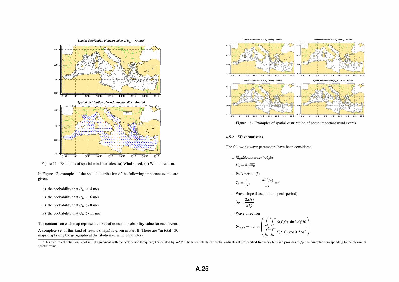
4

4

5

5

5

5

5

5

5 5

5

5

5

5.5

5.5

5.5

5.55.5

5.5

5.5

5.5

5.5

5.5

5.55.5

5.5

5.5

5.5

5.5

5.5

5.5

5.5

6

6

666

6

6

6

6

6

66.5

6.56.5

77.

5

45°N

5°W 0° 5°E 10°E 15°E 20°E 25°E 30°E 35°E30°N

35°N

40°N

Spatial distribution of mean value of UW

. Annual

30%

45°N

5°W 0° 5°E 10°E 15°E 20°E 25°E 30°E 35°E30°N

35°N

40°N

Spatial distribution of wind directionality. Annual

Figure 11 - Examples of spatial wind statistics. (a) Wind speed, (b) Wind direction.

In Figure 12, examples of the spatial distribution of the following important events aregiven:

i) the probability that UW < 4 m/s

ii) the probability that UW < 6 m/s

iii) the probability that UW > 8 m/s

iv) the probability that UW > 11 m/s

The contours on each map represent curves of constant probability value for each event.

A complete set of this kind of results (maps) is given in Part B. There are “in total” 30maps displaying the geographical distribution of wind parameters.

20

25

25

25

25

25

30

30

30

30

30

30

30

30

35

35

35

35

35

35

35

35

35

35

35

35

35

3535

35

35

35

40

40

40

40

40

40

40

40

40

40

40

40

40

40

45°N

5°W 0° 5°E 10°E 15°E 20°E 25°E 30°E 35°E30°N

35°N

40°N

Spatial distribution of P[UW

< 4m/s]. Annual

50

50

50

50

60

60

60

60

60

60

60

60

60

60

60

60

60

60

60

60

60

60

60

70

70

70

70

70

70

7070

70

70

70

70

70

45°N

5°W 0° 5°E 10°E 15°E 20°E 25°E 30°E 35°E30°N

35°N

40°N

Spatial distribution of P[UW

< 6m/s]. Annual

10

10

10

15

15

15

15

15

15

15

15

15

15

15

15

15

20

20

20

20

20

20

20

20

20 2020

20 20

20

20

25

25

25

25

25

25

25

25

25

30

30

30

30

30

30 3540

45°N

5°W 0° 5°E 10°E 15°E 20°E 25°E 30°E 35°E30°N

35°N

40°N

Spatial distribution of P[UW

> 8m/s]. Annual

1

2

2

2

2

24

4

4

4

4

4

4

4

4

4

4

4

4

4

4

4

4

4

6

6

6

6

6

6

66

6

6

6

666

6

6

6

6

6

6

68

8

8

8

8

8

8

8

88

8

12

12

16

20

45°N

5°W 0° 5°E 10°E 15°E 20°E 25°E 30°E 35°E30°N

35°N

40°N

Spatial distribution of P[UW

> 11m/s]. Annual

Figure 12 - Examples of spatial distribution of some important wind events

4.5.2 Wave statistics

The following wave parameters have been considered:

– Significant wave height

HS = 4√

m0

– Peak period (6)

TP =1fP

,dS( fP)

d f= 0

– Wave slope (based on the peak period)

βP =2πHS

gT 2P

– Wave direction

Θwave = arctan

∫ 2π

0

∫ ∞

0S( f ,θ) sinθ d f dθ

∫ 2π

0

∫ ∞

0S( f ,θ) cosθ d f dθ

6This theoretical definition is not in full agreement with the peak period (frequency) calculated by WAM. The latter calculates spectral ordinates at prespecified frequency bins and provides as f P, the bin-value corresponding to the maximumspectral value.

A.25

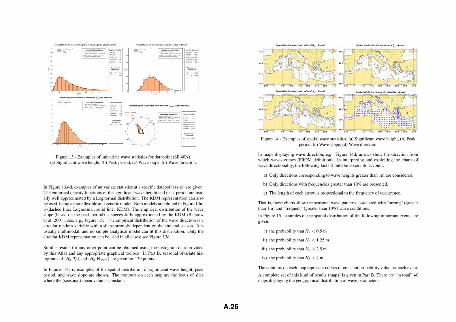
Probability density function of significant wave height HS (Sea and Swell)

Empirical Statistics

Mean Value

Stand. Dev.

Var. Coeff.

Skewness Coeff.

Kurtosis Coeff.

Sample Min

Sample Max

Parameters ofAnalytic PDF

KDE bW

LogN µσ

=

=

=

=

=

=

=

=

=

=

1.39

1.14

0.82

1.94

5.06

0.04

9.95

40 %

0.0326

0.7830

0 0.5 1 1.5 2 2.5 3 3.5 40

0.2

0.4

0.6

0.8

1

1.2

1.4

1.6

1.8

2

HS [m]

[1/m

]Empirical PDF Data point(s) identification

1. MED.33 (0.5) (40°N, 6°E)Period of observ. :1992.07.01 − 2002.06.30

Month(s) : 1, 2, 3, 4, 5, 6, 7, 8, 9, 10, 11, 12Total number of observations: 14608

KDELogN

Probability density function of peak period TP (Sea and Swell)

Empirical Statistics

Mean Value

Stand. Dev.

Var. Coeff.

Skewness Coeff.

Kurtosis Coeff.

Sample Min

Sample Max

Parameters ofAnalytic PDF

KDE bW

LogN µσ

=

=

=

=

=

=

=

=

=

=

6.54

1.95

0.30

0.55

0.35

2.28

21.62

120 %

1.8330

0.3037

0 2 4 6 8 10 12 140

0.1

0.2

0.3

0.4

0.5

TP [s]

[1/s

]

Empirical PDF Data point(s) identification1. MED.33 (0.5) (40°N, 6°E)

Period of observ. :1992.07.01 − 2002.06.30

Month(s) : 1, 2, 3, 4, 5, 6, 7, 8, 9, 10, 11, 12Total number of observations: 14608

KDELogN

Probability density function of wave slope βP (Sea and Swell)

Empirical Statistics

Mean Value

Stand. Dev.

Var. Coeff.

Skewness Coeff.

Kurtosis Coeff.

Sample Min

Sample Max

Parameters ofAnalytic PDF

KDE bW

=

=

=

=

=

=

=

=

1.87

0.80

0.43

0.63

0.17

0.04

6.26

60 %

0 0.5 1 1.5 2 2.5 3 3.5 4 4.5 5 5.5 6 6.5 70

0.1

0.2

0.3

0.4

0.5

0.6

0.7

0.8

0.9

1

βP [%]

Empirical PDF Data point(s) identification1. MED.33 (0.5) (40°N, 6°E)

Period of observ. :1992.07.01 − 2002.06.30

Month(s) : 1, 2, 3, 4, 5, 6, 7, 8, 9, 10, 11, 12Total number of observations: 14608

KDE

Polar histogram (%) of mean wave direction Θwave

(Sea and Swell)

Empirical Statistics

Mean Value

Stand. Dev.

Var. Coeff.

Skewness Coeff.

Kurtosis Coeff.

Sample Min

Sample Max

Parameters ofAnalytic PDF

KDE bW

=

=

=

=

=

=

=

=

319.42

83.91

−−−−−−

0.09

0.78

0.00

359.97

60 %

N

30o

60o

E

120o

150o

S210o

240o

W

300o

330o

10%

20%

30%

40%

Empirical

Data point(s) identification1. MED.33 (0.5) (40°N, 6°E) Period of observ.:1992.07.01 − 2002.06.30 Number of observations: 14608

Month(s) : 1, 2, 3, 4, 5, 6, 7, 8, 9, 10, 11, 12

KDE

Figure 13 - Examples of univariate wave statistics for datapoint (6E,40N).(a) Significant wave height, (b) Peak period, (c) Wave slope, (d) Wave direction.

In Figure 13a-d, examples of univariate statistics at a specific datapoint (site) are given.The empirical density functions of the significant wave height and peak period are usu-ally well approximated by a Lognormal distribution. The KDM representation can alsobe used, being a more flexible and generic model. Both models are plotted in Figure 13a-b (dashed line: Lognormal, solid line: KDM). The empirical distribution of the waveslope (based on the peak period) is successfully approximated by the KDM (Barstowet al, 2001); see, e.g., Figure 13c. The empirical distribution of the wave direction is acircular random variable with a shape strongly dependent on the site and season. It isusually multimodal, and no simple analytical model can fit this distribution. Only thecircular KDM representation can be used in all cases; see Figure 13d.

Similar results for any other point can be obtained using the histogram data providedby this Atlas and any appropriate graphical toolbox. In Part B, seasonal bivariate his-tograms of (HS,TP) and (HS,Θwave) are given for 129 points.

In Figures 14a-c, examples of the spatial distribution of significant wave height, peakperiod, and wave slope are shown. The contours on each map are the locus of siteswhere the (seasonal) mean value is constant.

0.6

0.8

0.8

0.8

0.8

0.8

0.8

0.80.8

0.8

1

1

1

1

1

1

1

1

1

1

1

1

1

1

1.2

1.2

1.2

1.2

1.2

1.2

1.2 1.2

1.2

1.2

1.2

1.41.4

45°N

5°W 0° 5°E 10°E 15°E 20°E 25°E 30°E 35°E30°N

35°N

40°N

Spatial distribution of mean value of HS . Annual

55

5.5

5.5 5.5

5.5

5.5

5.5

5.5

5.5

6

6 6

66

6

6

6

6

6

6

6

6

6.5

6.5

6.5

6.5

6.5

6.56.5

6.5

6.5

6.5

6.5

6.57

7

7

7

45°N

5°W 0° 5°E 10°E 15°E 20°E 25°E 30°E 35°E30°N

35°N

40°N

Spatial distribution of mean value of Tp . Annual

1.11.3

1.3

1.3

1.3

1.3

1.5

1.5

1.51.5

1.5

1.5

1.5

1.5

1.5

1.5

1.5

1.5

1.7

1.7

1.71.7

1.7

1.7

1.71.7

1.7

1.7

1.7

1.7

1.7

1.7

1.7

1.7

1.7

1.7

1.7

1.71.9

1.9

1.9

1.9

1.9

1.9

1.91.9

1.9

1.9

2.1

2.1

2.1

2.1

2.1

45°N

5°W 0° 5°E 10°E 15°E 20°E 25°E 30°E 35°E30°N

35°N

40°N

Spatial distribution of mean value of βp . Annual

30%

45°N

5°W 0° 5°E 10°E 15°E 20°E 25°E 30°E 35°E30°N

35°N

40°N

Spatial distribution of wave directionality. Annual

Figure 14 - Examples of spatial wave statistics. (a) Significant wave height, (b) Peakperiod, (c) Wave slope, (d) Wave direction.

In maps displaying wave direction, e.g. Figure 14d, arrows show the direction fromwhich waves comes (FROM definition). In interpreting and exploiting the charts ofwave directionality, the following facts should be taken into account:

a) Only directions corresponding to wave heights greater than 1m are considered,

b) Only directions with frequencies greater than 10% are presented,

c) The length of each arrow is proportional to the frequency of occurrence.

That is, these charts show the seasonal wave patterns associated with “strong” (greaterthan 1m) and “frequent” (greater than 10%) wave conditions.

In Figure 15, examples of the spatial distribution of the following important events aregiven:

i) the probability that HS < 0.5 m

ii) the probability that HS < 1.25 m

iii) the probability that HS > 2.5 m

iv) the probability that HS > 4 m

The contours on each map represent curves of constant probability value for each event.

A complete set of this kind of results (maps) is given in Part B. There are “in total” 40maps displaying the geographical distribution of wave parameters.

A.26

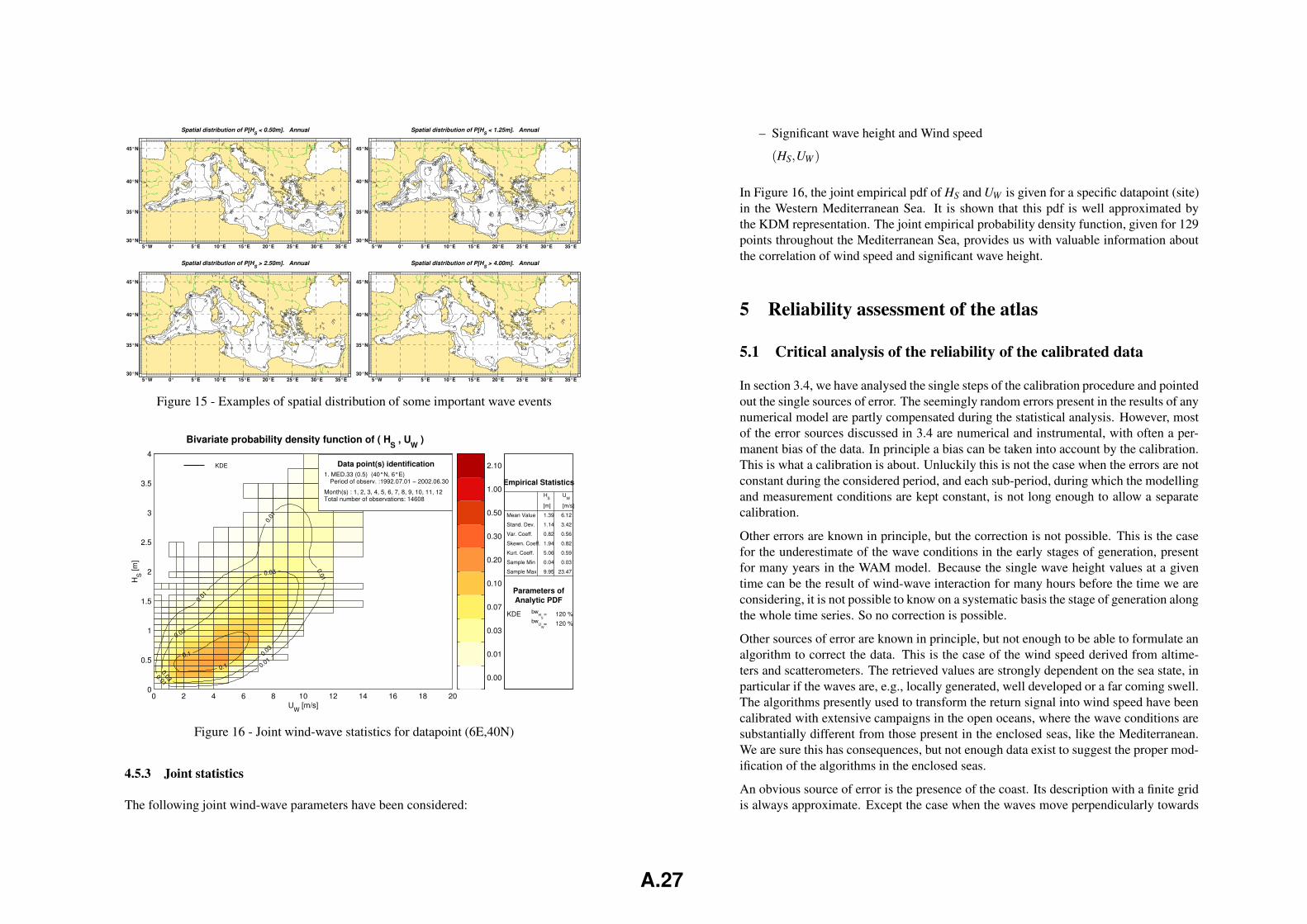
10

10

10

15

15

15

15

15

15

15

15

15

15

20

20

2020

20

20

20

20

20

2020

20

203030

30

30

30

30

30

3030

30

40

40

40

40

40

40

40

50

5050

50

50

60

60

70

45°N

5°W 0° 5°E 10°E 15°E 20°E 25°E 30°E 35°E30°N

35°N

40°N

Spatial distribution of P[HS < 0.50m]. Annual

55

60

60

65

65

65

65

65

65

65

65

65

65

65

65

70

70

70

70

70

70

70

70

70

70

70

75

75

75

75

75

75

75

75

75

75

75

75

75

75

75

80

80

8080

80

80

80

80

80

80

80

80

85

85

85

85

85

90

90

45°N

5°W 0° 5°E 10°E 15°E 20°E 25°E 30°E 35°E30°N

35°N

40°N

Spatial distribution of P[HS < 1.25m]. Annual

1.5

1.5

1.5

1.5

2.5

2.5

2.5

2.5

2.52.5

2.5

2.5

2.5

2.5

2.5

2.5

2.5

5

55

5

55

5

5

5

5

5

5

5

5

5

55

7.5

7.5

7.5

7.5

7.5

7.5

7.5

7.5

10

10

10

10

10

15

45°N

5°W 0° 5°E 10°E 15°E 20°E 25°E 30°E 35°E30°N

35°N

40°N

Spatial distribution of P[HS > 2.50m]. Annual

0.1

0.1

0.1

0.1

0.1

0.10.5

0.5

0.5

0.5

0.5

0.5

0.5

0.5

0.5

0.5

0.5

0.5

0.5

0.5

0.5

0.5

0.5

0.5

0.5

0.5

0.5

0.5

1

1

1 1

1

11

1

11

1

22

22

4 4

45°N

5°W 0° 5°E 10°E 15°E 20°E 25°E 30°E 35°E30°N

35°N

40°N

Spatial distribution of P[HS > 4.00m]. Annual

Figure 15 - Examples of spatial distribution of some important wave events

0.00

0.01

0.03

0.07

0.10

0.20

0.30

0.50

1.00

2.10

Empirical StatisticsH

SU

W

[m] [m/s]

Mean Value

Stand. Dev.

Var. Coeff.

Skewn. Coeff.

Kurt. Coeff.

Sample Min

Sample Max

Parameters ofAnalytic PDF

KDE bwH

Sbw

UW

=

=

1.39

1.14

0.82

1.94

5.06

0.04

9.95

6.12

3.42

0.56

0.82

0.59

0.03

23.47

120 %120 %

0 2 4 6 8 10 12 14 16 18 200

0.5

1

1.5

2

2.5

3

3.5

4

0.1

0.1 0.03

0.03

0.03

0.03

0.01

0.01

0.01

0.01

0.01

1. MED.33 (0.5) (40°N, 6°E)

Month(s) : 1, 2, 3, 4, 5, 6, 7, 8, 9, 10, 11, 12

Data point(s) identification

Period of observ. :1992.07.01 − 2002.06.30

Total number of observations: 14608

KDE

UW

[m/s]

Bivariate probability density function of ( HS , U

W )

HS [m

]

Figure 16 - Joint wind-wave statistics for datapoint (6E,40N)

4.5.3 Joint statistics

The following joint wind-wave parameters have been considered:

– Significant wave height and Wind speed

(HS,UW )

In Figure 16, the joint empirical pdf of HS and UW is given for a specific datapoint (site)in the Western Mediterranean Sea. It is shown that this pdf is well approximated bythe KDM representation. The joint empirical probability density function, given for 129points throughout the Mediterranean Sea, provides us with valuable information aboutthe correlation of wind speed and significant wave height.

5 Reliability assessment of the atlas

5.1 Critical analysis of the reliability of the calibrated data

In section 3.4, we have analysed the single steps of the calibration procedure and pointedout the single sources of error. The seemingly random errors present in the results of anynumerical model are partly compensated during the statistical analysis. However, mostof the error sources discussed in 3.4 are numerical and instrumental, with often a per-manent bias of the data. In principle a bias can be taken into account by the calibration.This is what a calibration is about. Unluckily this is not the case when the errors are notconstant during the considered period, and each sub-period, during which the modellingand measurement conditions are kept constant, is not long enough to allow a separatecalibration.

Other errors are known in principle, but the correction is not possible. This is the casefor the underestimate of the wave conditions in the early stages of generation, presentfor many years in the WAM model. Because the single wave height values at a giventime can be the result of wind-wave interaction for many hours before the time we areconsidering, it is not possible to know on a systematic basis the stage of generation alongthe whole time series. So no correction is possible.

Other sources of error are known in principle, but not enough to be able to formulate analgorithm to correct the data. This is the case of the wind speed derived from altime-ters and scatterometers. The retrieved values are strongly dependent on the sea state, inparticular if the waves are, e.g., locally generated, well developed or a far coming swell.The algorithms presently used to transform the return signal into wind speed have beencalibrated with extensive campaigns in the open oceans, where the wave conditions aresubstantially different from those present in the enclosed seas, like the Mediterranean.We are sure this has consequences, but not enough data exist to suggest the proper mod-ification of the algorithms in the enclosed seas.

An obvious source of error is the presence of the coast. Its description with a finite gridis always approximate. Except the case when the waves move perpendicularly towards

A.27

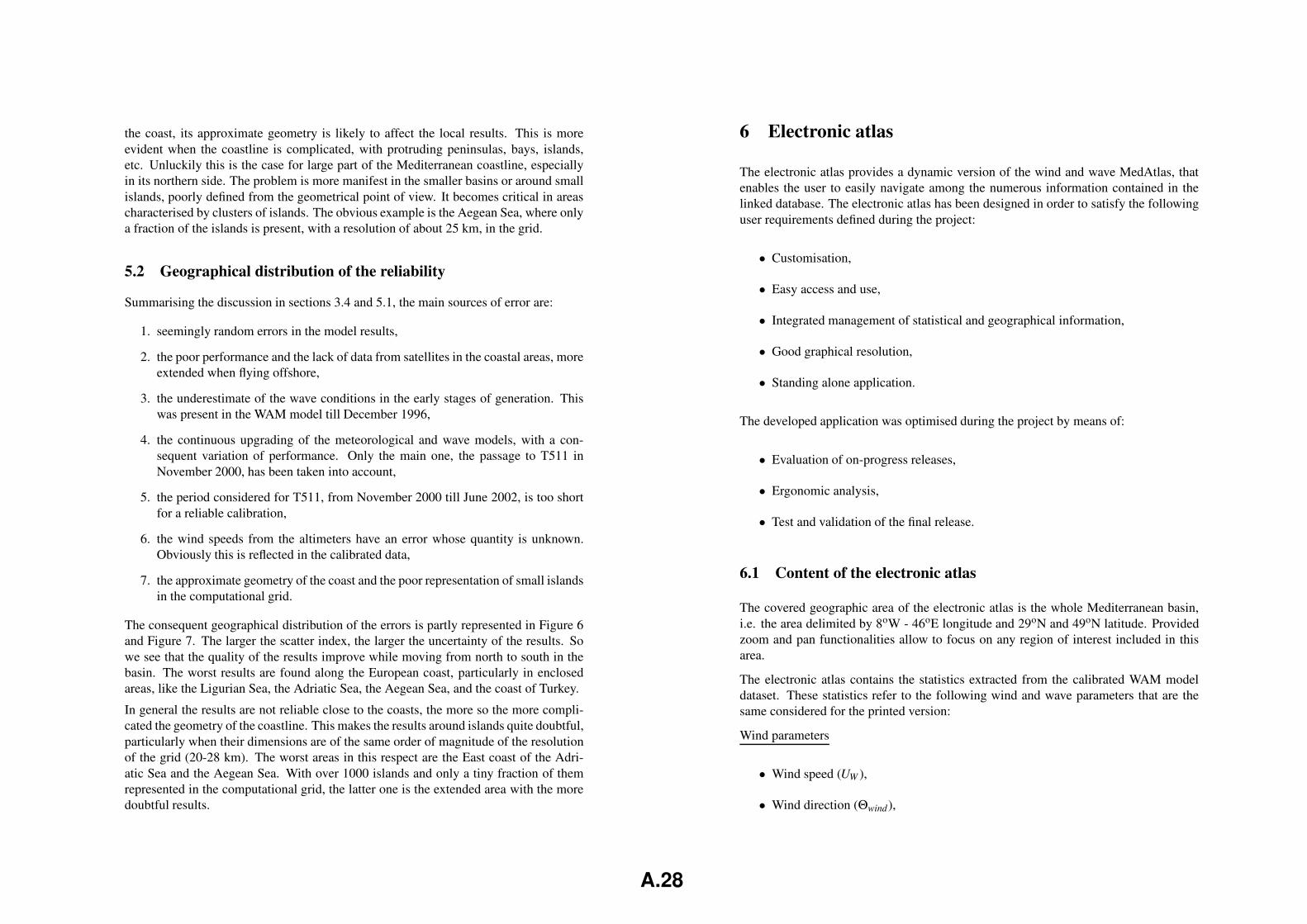
the coast, its approximate geometry is likely to affect the local results. This is moreevident when the coastline is complicated, with protruding peninsulas, bays, islands,etc. Unluckily this is the case for large part of the Mediterranean coastline, especiallyin its northern side. The problem is more manifest in the smaller basins or around smallislands, poorly defined from the geometrical point of view. It becomes critical in areascharacterised by clusters of islands. The obvious example is the Aegean Sea, where onlya fraction of the islands is present, with a resolution of about 25 km, in the grid.

5.2 Geographical distribution of the reliability

Summarising the discussion in sections 3.4 and 5.1, the main sources of error are:

1. seemingly random errors in the model results,

2. the poor performance and the lack of data from satellites in the coastal areas, moreextended when flying offshore,

3. the underestimate of the wave conditions in the early stages of generation. Thiswas present in the WAM model till December 1996,

4. the continuous upgrading of the meteorological and wave models, with a con-sequent variation of performance. Only the main one, the passage to T511 inNovember 2000, has been taken into account,

5. the period considered for T511, from November 2000 till June 2002, is too shortfor a reliable calibration,

6. the wind speeds from the altimeters have an error whose quantity is unknown.Obviously this is reflected in the calibrated data,

7. the approximate geometry of the coast and the poor representation of small islandsin the computational grid.

The consequent geographical distribution of the errors is partly represented in Figure 6and Figure 7. The larger the scatter index, the larger the uncertainty of the results. Sowe see that the quality of the results improve while moving from north to south in thebasin. The worst results are found along the European coast, particularly in enclosedareas, like the Ligurian Sea, the Adriatic Sea, the Aegean Sea, and the coast of Turkey.

In general the results are not reliable close to the coasts, the more so the more compli-cated the geometry of the coastline. This makes the results around islands quite doubtful,particularly when their dimensions are of the same order of magnitude of the resolutionof the grid (20-28 km). The worst areas in this respect are the East coast of the Adri-atic Sea and the Aegean Sea. With over 1000 islands and only a tiny fraction of themrepresented in the computational grid, the latter one is the extended area with the moredoubtful results.

6 Electronic atlas

The electronic atlas provides a dynamic version of the wind and wave MedAtlas, thatenables the user to easily navigate among the numerous information contained in thelinked database. The electronic atlas has been designed in order to satisfy the followinguser requirements defined during the project:

• Customisation,

• Easy access and use,

• Integrated management of statistical and geographical information,

• Good graphical resolution,

• Standing alone application.

The developed application was optimised during the project by means of:

• Evaluation of on-progress releases,

• Ergonomic analysis,

• Test and validation of the final release.

6.1 Content of the electronic atlas

The covered geographic area of the electronic atlas is the whole Mediterranean basin,i.e. the area delimited by 8oW - 46oE longitude and 29oN and 49oN latitude. Providedzoom and pan functionalities allow to focus on any region of interest included in thisarea.

The electronic atlas contains the statistics extracted from the calibrated WAM modeldataset. These statistics refer to the following wind and wave parameters that are thesame considered for the printed version:

Wind parameters

• Wind speed (UW ),

• Wind direction (Θwind),

A.28

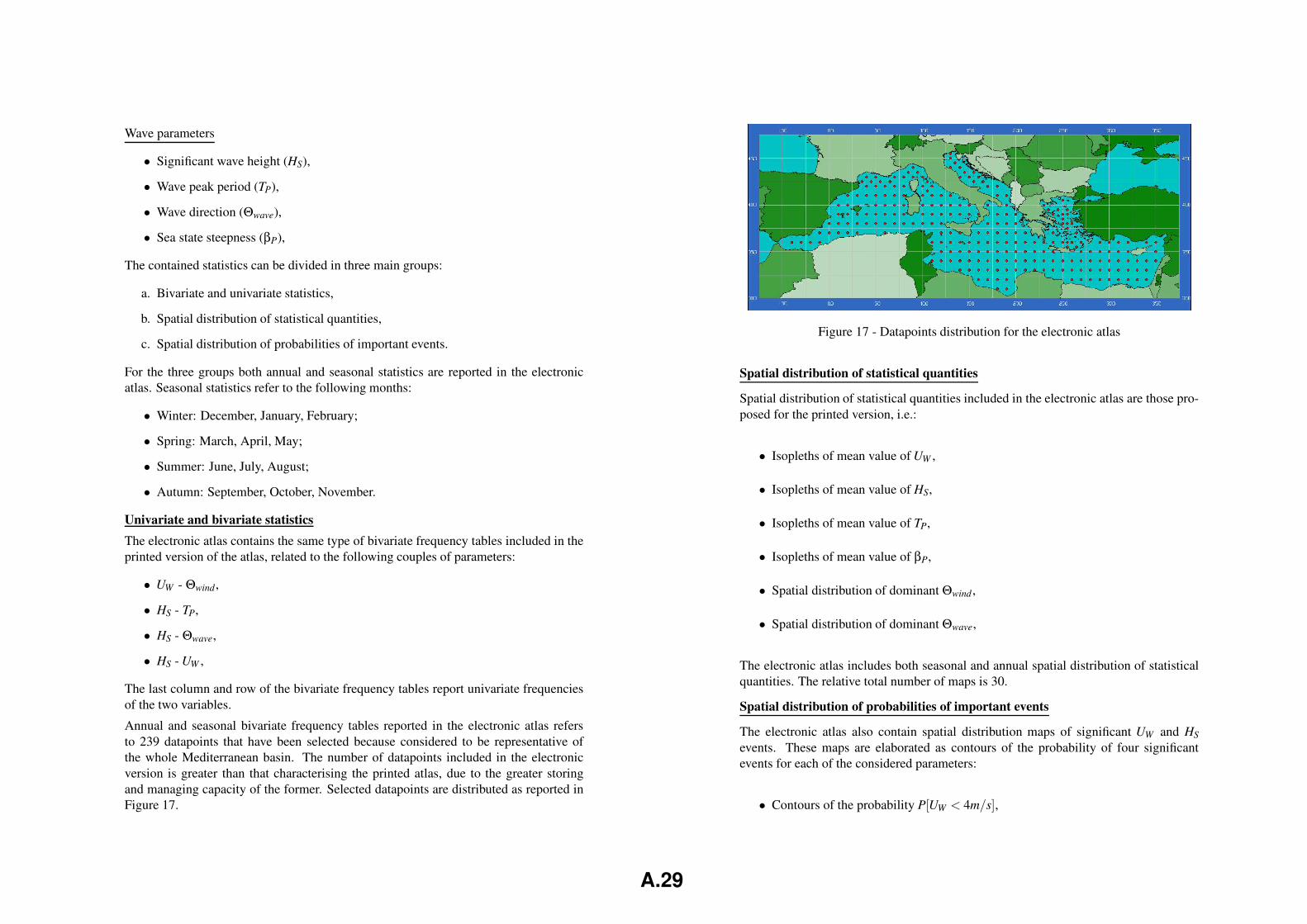
Wave parameters

• Significant wave height (HS),

• Wave peak period (TP),

• Wave direction (Θwave),

• Sea state steepness (βP),

The contained statistics can be divided in three main groups:

a. Bivariate and univariate statistics,

b. Spatial distribution of statistical quantities,

c. Spatial distribution of probabilities of important events.

For the three groups both annual and seasonal statistics are reported in the electronicatlas. Seasonal statistics refer to the following months:

• Winter: December, January, February;

• Spring: March, April, May;

• Summer: June, July, August;

• Autumn: September, October, November.

Univariate and bivariate statisticsThe electronic atlas contains the same type of bivariate frequency tables included in theprinted version of the atlas, related to the following couples of parameters:

• UW - Θwind ,

• HS - TP,

• HS - Θwave,

• HS - UW ,

The last column and row of the bivariate frequency tables report univariate frequenciesof the two variables.

Annual and seasonal bivariate frequency tables reported in the electronic atlas refersto 239 datapoints that have been selected because considered to be representative ofthe whole Mediterranean basin. The number of datapoints included in the electronicversion is greater than that characterising the printed atlas, due to the greater storingand managing capacity of the former. Selected datapoints are distributed as reported inFigure 17.

Figure 17 - Datapoints distribution for the electronic atlas

Spatial distribution of statistical quantities

Spatial distribution of statistical quantities included in the electronic atlas are those pro-posed for the printed version, i.e.:

• Isopleths of mean value of UW ,

• Isopleths of mean value of HS,

• Isopleths of mean value of TP,

• Isopleths of mean value of βP,

• Spatial distribution of dominant Θwind ,

• Spatial distribution of dominant Θwave,

The electronic atlas includes both seasonal and annual spatial distribution of statisticalquantities. The relative total number of maps is 30.

Spatial distribution of probabilities of important events

The electronic atlas also contain spatial distribution maps of significant UW and HSevents. These maps are elaborated as contours of the probability of four significantevents for each of the considered parameters:

• Contours of the probability P[UW < 4m/s],

A.29

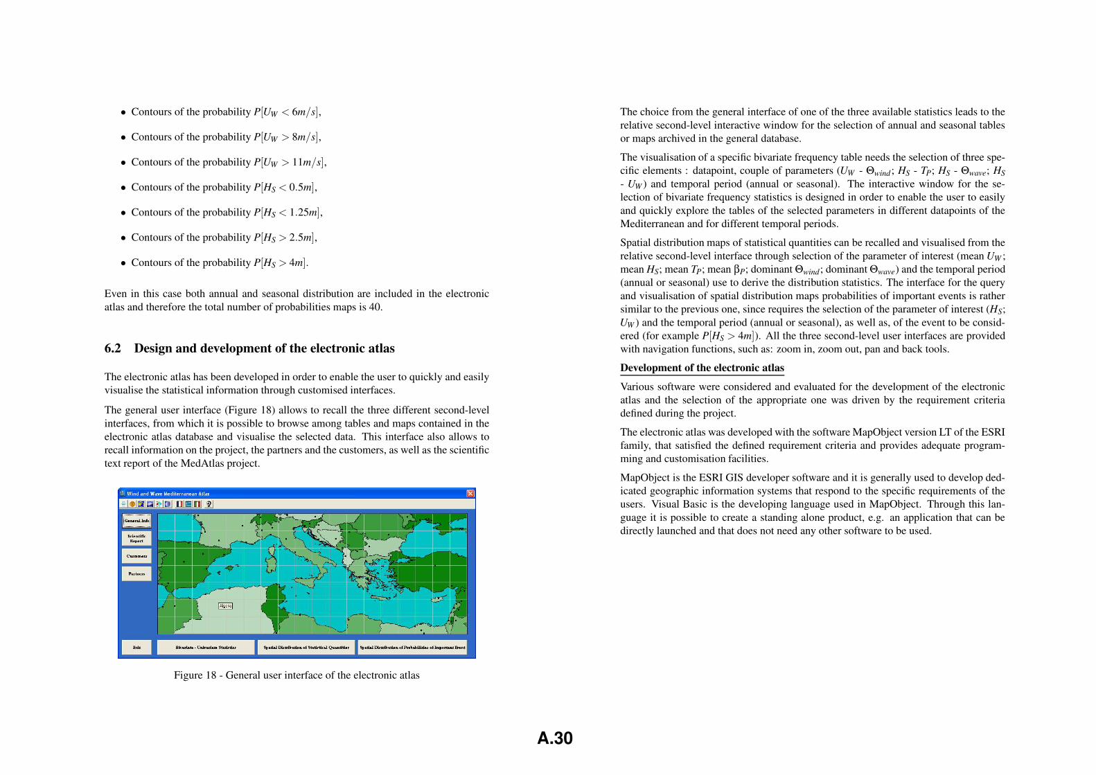
• Contours of the probability P[UW < 6m/s],

• Contours of the probability P[UW > 8m/s],

• Contours of the probability P[UW > 11m/s],

• Contours of the probability P[HS < 0.5m],

• Contours of the probability P[HS < 1.25m],

• Contours of the probability P[HS > 2.5m],

• Contours of the probability P[HS > 4m].

Even in this case both annual and seasonal distribution are included in the electronicatlas and therefore the total number of probabilities maps is 40.

6.2 Design and development of the electronic atlas

The electronic atlas has been developed in order to enable the user to quickly and easilyvisualise the statistical information through customised interfaces.

The general user interface (Figure 18) allows to recall the three different second-levelinterfaces, from which it is possible to browse among tables and maps contained in theelectronic atlas database and visualise the selected data. This interface also allows torecall information on the project, the partners and the customers, as well as the scientifictext report of the MedAtlas project.

Figure 18 - General user interface of the electronic atlas

The choice from the general interface of one of the three available statistics leads to therelative second-level interactive window for the selection of annual and seasonal tablesor maps archived in the general database.

The visualisation of a specific bivariate frequency table needs the selection of three spe-cific elements : datapoint, couple of parameters (UW - Θwind ; HS - TP; HS - Θwave; HS- UW ) and temporal period (annual or seasonal). The interactive window for the se-lection of bivariate frequency statistics is designed in order to enable the user to easilyand quickly explore the tables of the selected parameters in different datapoints of theMediterranean and for different temporal periods.

Spatial distribution maps of statistical quantities can be recalled and visualised from therelative second-level interface through selection of the parameter of interest (mean UW ;mean HS; mean TP; mean βP; dominant Θwind; dominant Θwave) and the temporal period(annual or seasonal) use to derive the distribution statistics. The interface for the queryand visualisation of spatial distribution maps probabilities of important events is rathersimilar to the previous one, since requires the selection of the parameter of interest (HS;UW ) and the temporal period (annual or seasonal), as well as, of the event to be consid-ered (for example P[HS > 4m]). All the three second-level user interfaces are providedwith navigation functions, such as: zoom in, zoom out, pan and back tools.

Development of the electronic atlas

Various software were considered and evaluated for the development of the electronicatlas and the selection of the appropriate one was driven by the requirement criteriadefined during the project.

The electronic atlas was developed with the software MapObject version LT of the ESRIfamily, that satisfied the defined requirement criteria and provides adequate program-ming and customisation facilities.

MapObject is the ESRI GIS developer software and it is generally used to develop ded-icated geographic information systems that respond to the specific requirements of theusers. Visual Basic is the developing language used in MapObject. Through this lan-guage it is possible to create a standing alone product, e.g. an application that can bedirectly launched and that does not need any other software to be used.

A.30

Bibliography

[1] Aivazian, S., Enukov, I., Mechalkine, L., 1986, Elements de modelisation et traite-ment primaire des donnees, MIR Publishers, Moscow.

[2] Andrew, R.N. and W.G. Price, 1978, Applications of generalized gamma functionsin ship dynamics, Trans. Royal Inst. Naval Architects (RINA), 1978, pp. 137-143.

[3] Athanassoulis, G.A. and Ch.N. Stefanakos, 1995, A nonstationary stochasticmodel for long-term time series of significant wave height, Journal of Geophys-ical Research, Vol. 100, No. C8, pp. 16149-16162.

[4] Athanassoulis G.A. and Ch.N. Stefanakos, 1996a, ”Statistical analysis of wavedata. Ia: Univariate statistics/Mediterranean Sea”, NTUA Report, WERATLASProject, JOU2-CT93-0390, 35+85+85pp.

[5] Athanassoulis, G.A. and Ch.N. Stefanakos, 1996b, Statistical Analysis of wavedata. IIa: Bivariate statistics/Mediterranean Sea, NTUA Report, WERATLASProject, JOU2-CT93-0390, April 1996.

[6] Athanassoulis, G.A. and Ch.N. Stefanakos, 1996c, Statistical analysis of wavedata. IIIa: Directional statistics/Mediterranean Sea. Part 1: Theoretical back-ground, Greek contribution to WERATLAS project, JOU2-CT93-0390, May 1996.

[7] Athanassoulis, G.A. and Ch.N. Stefanakos, 1998, Missing-value completion ofnonstationary time series of wave data, 17th International Conference on OffshoreMechanics and Arctic Engineering, Lisbon, Portugal, July 5-9, 1998.

[8] Athanassoulis G.A., Stefanakos, Ch.N., 2001, ”Time Series Statistics”, Greekcontribution to MEDATLAS project, Contract No. 99/RFP10.10/009, July 2001(70pp.).

[9] Athanassoulis, G.A. and K.A. Belibassakis, 1999, Analytic representation of mul-tivariate distributions by means of kernel density models with application to oceanwave data,EUROWAVES project report no. SCR/18, MAS3-CT97-0109, July1999.

[10] Athanassoulis, G.A. Belibassakis, K.A., 2002, ”Probabilistic description of meto-cean parameters by means of kernel density models. 1. Theoretical backgroundand first results”, Applied Ocean Research, Vol. 24, pp. 1-20.

[11] Athanassoulis, G.A. E.K. Skarsoulis and K.A. Belibassakis, 1994, Bivariate dis-tributions with given marginals with an application to wave climate description,Applied Ocean Research, Vol. 16, No. 1, pp. 1-17.

[12] Athanassoulis, G.A. E.K. Skarsoulis, 1992, Wind and Wave Atlas of the North-Eastern Mediterranean Sea, Ship and Marine Hydrodynamics Laboratory, NationalTechnical University of Athens.

[13] Athanassoulis, G.A., Vranas,P. and T.S. Soukissian, 1992, A new model for long-term stochastic analysis and prediction–Part I: Theoretical background, Journal ofShip Research, Vol. 36, No. 1, pp. 1-16.

[14] Barstow, S.F., G.A. Athanassoulis, L. Cavaleri, G. Mork, K.A. Belibassakis, Ch.N.Stefanakos, Th.P. Gerostathis, M. Sclavo, L. Bertotti, and H.E. Krogstad, 2001,EUROWAVES: A user-friendly tool for the evaluation of wave conditions at anyEuropean coastal location, Mast3 Project CT97-0109, Final technical Report.

[15] Belberova, D., and D. Myrhaug, 1996, Critical assessment of the joint occurrenceof wind and waves at a buoy station off the southern Norwegian coast, Journal ofWind Engineering and Industrial Aerodynamics, Vol. 61, 207-224.

[16] Bidlot, J.R., D.H.Holmes, P.A.Wittmann, R.Lalbeharry, and H.S.Chen, 2001, ”In-tercomparison of the performance of operational ocean wave forecasting systemswith buoy data”, ECMWF, Tech.Memo 315, 46pp.

[17] Bitner-Gregersen, E.M. and E.H. Cramer, 1995, Uncertainties of load character-istics and fatigue damage of ship structures, Marine Structures, 1995, No. 8, pp.97-117.

[18] Bitner-Gregersen, E.M., C. Guedes Soares and A. Silvestre, 1998, On the aver-age wave steepness, Ocean Wave Kinematics, Dynamics and Loads on Structures,Proc. of the 1998 International OTRC Symposium, April 30 -May 1, 1998, pp.513-520, Houston, Texas.

[19] Bitner-Gregersen, E.M., C.G. Soares, U. Machado and P. Cavaco, 1998, Com-parison of different approaches to joint environmental modelling, Proceedings ofthe 17th International Conference on Offshore Mechanics and Arctic Engineering,OMAE, Lisbon, Portugal, 5-9 July, 1998

[20] Cavaleri, L., and L.Bertotti, 2003a, The characteristics of wind and wave fieldsmodelled with different resolutions, Q.J.R.Meteorol.Soc., 129, pp.1647-1662.

[21] Cavaleri, L., and L.Bertotti, 2003b, The accuracy of modelled wind and wave fieldsin enclosed seas, in publication on Tellus.

A.31

[22] Cavaleri, L., Bertotti, L., Sclavo, M., 2000, Comparison between model and buoymeasured wave parameters, ISDGM Report, 2000.

[23] Cavaleri, L., Bertotti, L., Sclavo, M., Ramieri, E., 2002, Calibration of wind andwave model data in the Mediterranean Sea - The extended period July 1992 - June2002, ISDGM Report, 2002.

[24] Cavaleri, L., L.Bertotti, and P.Lionello, 1991, Wind wave cast in the MediterraneanSea, J.Geophys.Res., 96, No.C6, pp.10,739-10,764.

[25] Challenor, P. G., and O. D. Cotton, (1997), The SOC contribution to the ESAworking group calibration and validation of ERS-2 FD measurements of signifi-cant wave height and wind speed. In ”Proceedings CEOS Wind and wave valida-tion workshop”, pp. 81-93, 3-5 June, 1997, ESTEC , Noordwijk, The Netherlands

[26] Chen, S.X., 1999, Beta kernel estimators for density functions, ComputationalStatistics and Data Analysis, Vol. 31, pp. 131-145.

[27] Cotton, P. D., Challenor, P. G., and D. J. T. Carter (1997). An assessment of theaccuracy and reliablility of Geosat, ERS-1, ERS-2, and TOPEX altmeter measure-ments of significant wave height and wind speed. In ”Proceedings CEOS Wind andwave validation workshop”, pp. 81-93, 3-5 June, 1997, ESTEC , Noordwijk, TheNetherlands.

[28] Dacunha, N.M.C., M. Hogben and K.S. Andrews, 1984, Wave climate synthe-sis worldwide, Proc. of International Symposium on Wave and Wind ClimatologyWorldwide, The Royal Inst. of Naval Architects (RINA), 1984, London.

[29] De Boni, M., L.Cavaleri, and A.Rusconi, 1993, ”The Italian wave measure-ment network”, 23rd Int.Conf.Coast.Eng., pp.116-128, 4-9 October 1992, Venice,3520pp.

[30] Dell’Osso, L., L.Bertotti, and L.Cavaleri, 1992, The GORBUSH storm in theMediterranean Sea: atmospheric and wave simulation, Monthly Weather Review,120, No.1, pp.77-90.

[31] Direccion General de Puertos y Costas, 1988, Atlas Basado sobre ObservacionesVisuales de Barcos en Ruta.

[32] ERS user handbook ESA SP 11-48.

[33] Fang, Z., Dai Shunsun and Jin Chengyi, 1989, On the long-term joint distributionof characteristic wave height and period and its application, Acta OceanologicaSinica, Vol. 8, No. 3, pp. 315-325.

[34] Fang, Z.S. and N. Hogben, 1982, Analysis and Prediction of Long-term Probabil-ity Distributions of Wave Heights and Periods, Report, National Maritime Institute,1982, London.

[35] Feld, G. and J. Wolfram, 1996, Bivariate modelling of H and T , 15th InternationalOffshore Mechanics and Arctic Engineering Conference, 1996, Vol. 2, Florence,Italy.

[36] Ferreira, J.A. and C. Guedes Soares, 1999, Modelling the long-term distributionof significant wave height with the Beta and Gamma models, Ocean Engineering,Vol. 26, pp. 713-725.

[37] Fisher, N.I. 1993, Statistical Analysis of Circular Data, Cambridge UniversityPress, Cambridge, 1993.

[38] Fix, E. and Hodges, J.L., 1951, Nonparametric discrimination: Consistency prop-erties, Rep. No4, USAF School of Aviation Medicine, Randolph Field, Texas.

[39] Goda, Y. 2000, Random seas and design of maritime structures, World Scientific.

[40] Gran, S., 1992, A Course in Ocean Engineering, Elsevier Scence Publishers, Am-sterdam.

[41] Hardle, W., 1991, Smoothing techniques with implementation in S, Springer Ver-lag.

[42] Haver, S., 1985, Wave climate off northern Norway”, Applied Ocean Research,Vol. 7, 85-92.

[43] Hogben, N., 1990, Long term wave statistics, The Sea, (Le Mehaute, B. and D.M.Hanes, eds.), J. Wiley & Sons, New York, Vol. 9A, 293-333.

[44] Hogben, N., Dacunha and Ollivier, 1986, Global Wave Statistics.

[45] IAHR working group, 1989, List of sea-state parameters, Journal of Waterway,Port, Coastal, and Ocean Engineering, Vol. 115, No. 6, pp. 793-808, 1989.

[46] Ivchenko, G., Medvedev, Yu., 1990, Mathematical statistics, MIR Publishers,Moscow.

[47] Janssen, P.A.E.M., 1998, On error growth in wave models, Tech.Memo. No.249,ECMWF, 12pp.

[48] Jasper, N.H., 1956, Statistical distribution patterns of ocean waves and of wave-induced ship stresses and motions with engineering applications”, Transactions ofThe Society of Naval Architects and Marine Engineers, 1956, Vol. 64, pp. 375-432.

[49] Johnson, N., Kotz, S., 1970, Continuous univariate distributions, Houghton MifflinCo., Boston.

A.32

[50] Komen, G.J., L.Cavaleri, M.Donelan, K.Hasselmann, S.Hasselmann, andP.A.E.M.Janssen, 1994, Dynamics and Modelling of Ocean Waves, CambridgeUniversity Press, 536pp.

[51] Krogstad, H.E., 1985, Height and period distributions of extreme waves, AppliedOcean Research, Vol. 7, No. 3, pp. 158-165.

[52] Lefevre J.-M. and Cotton D., 2001. “Ocean Surface Waves”, in Fu, L.L., andCazenave, A., editors, Satellite Altimetry and Earth Sciences”, Academic Press,International Geophysics Series, Vol 69, 463p.

[53] Longuet-Higgins, M.S, Cartwright, D.E. and N.D. Smith, 1963, Observations ofthe directional spectrum of sea waves using the motion of a floating buoy in: OceanWave Spectra, Prentice-Hall, pp. 111-136.

[54] Longuet-Higgins, M.S., 1957, The statistical analysis of a random, moving sur-face, Philosophical Transactions of the Royal Society of London, Series A, Vol.249, pp. 321-387.

[55] Mardia, K.V., 1972, Statistics of directional data, Academic Press.

[56] Mathiesen, J. and E. Bitner-Gregersen, E., 1990, Joint distributions for significantwave height and wave zero-upcrossing period, Applied Ocean Research, 1990, Vol.12, pp. 93-103.

[57] Moerk G. and S.F. Barstow, 1998a, Comparison of WAM estimates of Hs withTOPEX/POSEIDON altimeter data in the Mediterranean Sea; a comparison of lowand high resolution wind models, EUROWAVES project report no.SCR/1 MAS3-CT97-0109, July 1998.

[58] Moerk G. and S.F. Barstow, 1998b, Comparison of WAM estimates of Hs withTOPEX/POSEIDON altimeter data in European Atlantic waters; a comparisonof low and high resolution wind models, EUROWAVES project report no.SCR/2,MAS3-CT97-0109, September 1998.

[59] Moerk G. and S.F. Barstow, 1999, Comparison of WAM estimates of Hs withTOPEX altimeter data in the Baltic and Black Sea, EUROWAVES project reportno. SCR/31, MAS3-CT97-0109, March 1999.

[60] Monbet, V., M. Prevosto and J. Deshayes, 1995, Approximation of up crossing ofhigh level for the acceleration of the response of a non linear stochastic oscillator,7th International Conference of Applications of Statistics and Probability, Paris.

[61] Naval Oceanography Command Detachment, 1983, U.S. Navy Hindcast SpectralOcean Wave Model Climatic Atlas: North-Atlantic Ocean.

[62] Nordenstrom, N., 1969, Methods for predicting long-term distributions of waveloads and probability of failure for ships. Part I: Environmental conditions andshort term response, Report 69-21-S, Det Norske Veritas.

[63] Ochi, M.K. 1998 Ocean waves. The stochastic approach, Cambridge UniversityPress

[64] Ochi, M.K., 1978, Wave statistics for the design of ships and ocean structures,Transactions of The Society of Naval Architects and Marine Engineers, 1978, Vol.60, pp. 47-76.

[65] Ochi, M.K., 1982, Stochastic analysis and probabilistic prediction of random seas,Advances in Hydroscience, Vol. 13, pp. 217-375, 1982.

[66] Parzen, E., 1962, On estimation of a probability density function and mode, TheAnnals of Mathematical Statistics, Vol. 33, No. 3, pp. 1065-1076.

[67] Philips, O.M., 1977, The dynamics of the upper ocean, Cambridge University Press(2nd edition).

[68] Plackett, R.L., 1965, A class of bivariate distributions. J. Am. Statist. Assoc., Vol.60, 516-522.

[69] Queffeulou P, 1996, Significant wave height and backscatter coefficient at ERS1/2and TOPEX-POSEIDON ground-track crossing points FDP, Final report, ESAcontract 143189, Department d’Oceanographie Spatial, IFREMER.

[70] Queffeulou P., A. Bentamy, Y. Quilfen and J. Tournadre, Validation of ERS-1 andTOPEX-POSEIDON altimeter wind and wave measurements, Document de travailDRO-OS 94-08, Ifremer, Decembre 1994.

[71] Scott, D.W., 1992, Multivariate density estimation. Theory, Practice and Visuali-sation, John Wiley & Sons.

[72] Silverman, B.W., 1986, Density estimation, Chapman and Hall.

[73] Simmons, A., 1991: Development of the operational 31-level T213 version of theECMWF forecast model, ECMWF Newsletter, 56, pp.3-13.

[74] Simmons, A., R.Mureau, and T.Petroliagis, 1995: Error growth and predictabilityestimates for the ECMWF forecasting system, Q.J.Roy.Meteor.Soc., 121, pp.1739-1771.

[75] Simonoff, J.S., 1996, Smoothing methods in statistics, Springer-Verlag.

[76] Soares, Guedes C., L.C. Lopes and M.D.S. Costa, 1988, Wave climate modellingfor engineering purposes, Proceedings of an International Conference on ComputerModelling in Ocean Engineering, B.A. Schrefler and O.C. Zienkiewicz (eds.),Venice, Italy, 19-23 September 1988, pp. 169-175.

A.33

[77] Stefanakos, Ch.N., 1999, Nonstationary stochastic modelling of time series withapplications to environmental data, Ph.D. Thesis, National Technical University ofAthens, Dept. of Naval Architecture and Marine Engineering, Athens, Greece.

[78] Stefanakos, Ch.N.,Athanassoulis, G.A., 2001, A unified methodology for the anal-ysis, completion and simulation of nonstationary time series with missing-values,with application to wave data, Applied Ocean Research, Vol. 23/4, pp. 207-220.

[79] Stefanakos, Ch.N., Athanassoulis, G.A., Barstow, S.F., 2002, Multiscale time se-ries modelling of significant wave height, 12th International Offshore and PolarEngineering Conference, ISOPE’2002, Kitakyushu, Japan, May 26-31, pp. 66-73.

[80] Stefanakos, Ch.N., Athanassoulis, G.A., 2003, Bivariate stochastic simulationbased on nonstationary time series modelling, 13th International Offshore and Po-lar Engineering Conference, ISOPE’2003, Honolulu, Hawaii, USA, May 25-31,pp. 46-50.

[81] Stefanakos, Ch.N., Athanassoulis, G.A., Cavaleri, L., Bertotti, L., Lefevre, J.-M.,2004a, Wind and Wave Climatology of the Mediterranean Sea. Part I: Wind Statis-tics, 14th International Offshore and Polar Engineering Conference, ISOPE’2004,Toulon, France, May 23-28.

[82] Stefanakos, Ch.N., Athanassoulis, G.A., Cavaleri, L., Bertotti, L., Lefevre, J.-M.,2004b, Wind and Wave Climatology of the Mediterranean Sea. Part II: Wave Statis-tics, 14th International Offshore and Polar Engineering Conference, ISOPE’2004,Toulon, France, May 23-28.

[83] Swail, V.R., and A.T.Cox, 2000, On the use of NCEP-NCAR reanalysis surfacemarine wind fields for a long-term North Atlantic wave hindcast, J.of Atmsph.And Ocean.Tech., Vol.17, pp.532-545.

[84] WAM-DI Group, 1988, The WAM model - a third generation ocean wave predic-tion model, J.Physic.Oceanog., 18, pp.1775-1810.

[85] Wand, M.P., Jones, M.C., 1995, Kernel smoothing, Chapman & Hall.

A.34