wind assisted propulsion for pure car and truck carriers

Wind assisted propulsion for pure

car and truck carriers

MÅRTEN S I LVAN IUS ma r t e n s i@k t h . s e

0 70 - 7713878

Master Thesis Ver. 1.1

KTH Centre for Naval Architecture

January 2009

ABSTRACT Several studies regarding wind assisted propulsion have been carried out before. The most common reasons for those studies have been high or increasing bunker prices. Most of the studies were never realized since the benefits, at that time, were too small. Due to environmental laws, public opinion and costs the modern shipping companies have to reduce their fuel consumption. This investigation focuses on reducing fuel consumption for a 230 m Pure Car and Truck Carrier using wind where five systems are examined. The systems are the Flettner rotor, the wing sail, the kite, the horizontal axle wind turbine and the vertical axle wind turbine. The Flettner rotor and the wing are mounted at the bow of the ship where profitable wind redirection and speed increasing occur. For these systems a global drag reducing effect due to delayed separation is also expected. However this effect is not considered in this study. Overall results conclude that the wing system is preferable. It has good payback investment, assumes to have global drag reducing effects, is cheap to build and maintain and has a predicted performance of 4.6% fuel saving on a worldwide route. The rotor could theoretically provide a fuel saving of 5.8% but is considered to have a more complicated installation. It also needs more free air volume than what’s available at the bow for full operability. The kite is an expensive installation and has poor payback on the investment. According to this model, and assumptions made, the kite performance is predicted to 5.0% fuel saving on a worldwide route. Wind turbines are not considered profitable.

3

ACKNOWLEDGEMENTS I would like to express my gratitude to the staff at the technical department at Wallenius Marine AB Stockholm office for their support and genuine effort to maintain a good working environment. My special thanks goes to the R&D group and Carl-Johan Söder for supporting and supervising this master thesis project. At the Royal Institute of technology (KTH) I would like to thank Anders Rosén at the Center for Naval Architecture for continuous review and support during my work. During the fluid mechanical investigation the support from Arne Karlsson at the mechanics institute were very helpful. CFD investigation could not have been done without the support of Stefan Wallin KTH Mechanics and Tristan Favre. Göran Gatenfjord at GGRail help me with wind turbine information and Christoph Thomsen-Jung at Skysails helped me with information about the Skysails system. At last I would like to thank the crew at M/V Undine for the professional reception and informational tour. Mårten Silvanius, Stockholm 2009-01-29

4

CONTENTS Nomenclature ................................................................................................................................................................ 5 1. Introduction .......................................................................................................................................................... 8

1.1. Objective ...................................................................................................................................................... 8 1.2. Method .......................................................................................................................................................... 8 1.3. Studied systems ........................................................................................................................................... 8 1.3.1. The Flettner Rotor ............................................................................................................................. 8 1.3.2. The kite ................................................................................................................................................ 9 1.3.3. The wing profile ................................................................................................................................. 9 1.3.4. Wind turbine .....................................................................................................................................10

1.4. Specifications of analyzed systems .........................................................................................................11 2. Studied ship .........................................................................................................................................................11

2.1. Advantages of the current ship shape ....................................................................................................12 2.2. Installation ..................................................................................................................................................13 2.2.1. Wing and rotor installation .............................................................................................................13 2.2.2. Kite installation ................................................................................................................................14

3. Modelling the system and ship performance .................................................................................................14 3.1. General sailing theory ...............................................................................................................................15 3.2. Total engine power needed .....................................................................................................................17 3.3. Modelling the bow ....................................................................................................................................21 3.4. System specific theory ..............................................................................................................................24 3.4.1. Flettner rotor ....................................................................................................................................24 3.4.2. The wing ............................................................................................................................................29 3.4.3. The Kite .............................................................................................................................................31 3.4.4. The horizontal axle wind turbine HAWT ....................................................................................34 3.4.5. The vertical axle wind turbine VAWT .........................................................................................35

3.5. Stability .......................................................................................................................................................37 3.6. Rudder induced resistance due to system .............................................................................................38

4. Results ..................................................................................................................................................................41 4.1. Bow effect ..................................................................................................................................................41 4.2. Power per square meter from systems ..................................................................................................41 4.3. Actual power from systems .....................................................................................................................42 4.4. Economic analysis .....................................................................................................................................44 4.4.1. Wind statistics ...................................................................................................................................44 4.4.2. Savings ...............................................................................................................................................45 4.4.3. Installation cost ................................................................................................................................45 4.4.4. Return on investment ......................................................................................................................46

5. Conclusion ...........................................................................................................................................................46 6. Recommendations ..............................................................................................................................................47 Appendix A – Result plots .........................................................................................................................................48 Appendix B – Wind data ............................................................................................................................................62 References.....................................................................................................................................................................64

5

NOMENCLATURE A projected area of system [m2]

FA frontal area of the ship [m2]

rA surface area of the rotor [m2]

RA surface area of the rudder [m2]

AR aspect ratio

RAR aspect ratio rudder

SA side area of the ship [m2]

b span [m]

B breadth of ship [m]

rotc rotational coefficient

BC block coefficient

lC lift coefficient

LC three dimensional lift coefficient

RLC three dimensional lift coefficient of rudder

dC drag coefficient

DC three dimensional lift coefficient

RDC three dimensional drag coefficient of rudder

fc frictional coefficient

pc wind turbine coefficient

xC drag coefficient of ship superstructure in x-direction

yC drag coefficient of ship superstructure in y-direction

d lever arm for the heeling tank [m]

D drag force [N]

kiteD drag force kite [N]

e span efficiency factor

fF frictional force [N]

xF force in x-direction [N]

HxAF aerodynamic hull force in x-direction [N]

SxAF system force in x-direction [N]

HxHF hydrodynamic hull force in x-direction [N]

PxHF hydrodynamic propulsion force in x-direction [N]

RxHF hydrodynamic rudder force in x-direction [N]

HSxAF added induced resistance due to side slip from system [N]

slipyHF added induced resistance due to side slip from hull [N]

yF force in y-direction [N]

SyAF system force in y-direction [N]

Sx totF total force generated by the system [N]

HyAF aerodynamic hull force in y-direction [N]

6

HyHF hydrodynamic hull force in y-direction [N]

RyHF hydrodynamic rudder force in y-direction [N]

ZF force in z-direction [N]

g gravity [m/s2]

h lever arm for wind system [m]

10mh altitude of 10 m [m]

rh height of the rotor [m]

systemh altitude of system [m]

HAWT Horizontal Axle Wind Turbine

DCk hull coefficient

1k hull coefficient

2k hull coefficient

L lift force [N]

kiteL lift force kite [N]

1 lL lift per length of rotor [N/m]

ppL Length between perpendiculars [m]

ReL characteristic length [m]

revM momentum required to spin the rotor [Nm]

P total engine power [W] p wind speed probability

PCTC Pure car truck carrier

revP power to rotate the rotor [W]

SP power from system [W]

turbP theoretical maximum output of wind turbine [W]

waveP power to compensate wave resistance [W]

windP power to compensate wind resistance [W]

rudderP power to compensate rudder resistance [W]

slipP power to compensate side slip from hull [W]

q stagnation pressure [kg/ms2]

r radius of the rotor [m]

Re Reynolds number

S swept area of wind turbine [m2] tdw tonne dead weight

T draft of ship [m]

rotU rotation speed rotor [m/s]

altV altitude dependent wind speed [m/s]

AV apparent wind speed [m/s]

~

AV corrected apparent wind speed [m/s]

dynAV kite dynamic wind speed [m/s]

kiteAV kite apparent wind speed [m/s]

VAWT Vertical Axle Wind Turbine

7

heelv volume heeling tank [m3]

TV true wind speed [m/s]

SV ship speed [m/s]

X global x-coordinate x ship x-coordinate

Y global y-coordinate y ship y-coordinate

'

vY non-dimensional manoeuvre derivative

vY dimensional manoeuvre derivative

δ system sheet angle [°]

ζ system mounting angle at hull [°]

λ yaw/drift angle [°]

β apparent wind direction [°]

localβ apparent wind direction at the bow[°]

γ true wind angle [°]

Γ circulation

θ heeling angle of kite [°] τ kite towing angle [°]

heelv heeling tank volume [m3]

Aρ density of air [kg/m2]

Hρ density of water [kg/m2]

shipη ship hull and propeller efficiency

σ constant according to Prandtl (7-14) µ dynamic viscosity of air

ω angular velocity

8

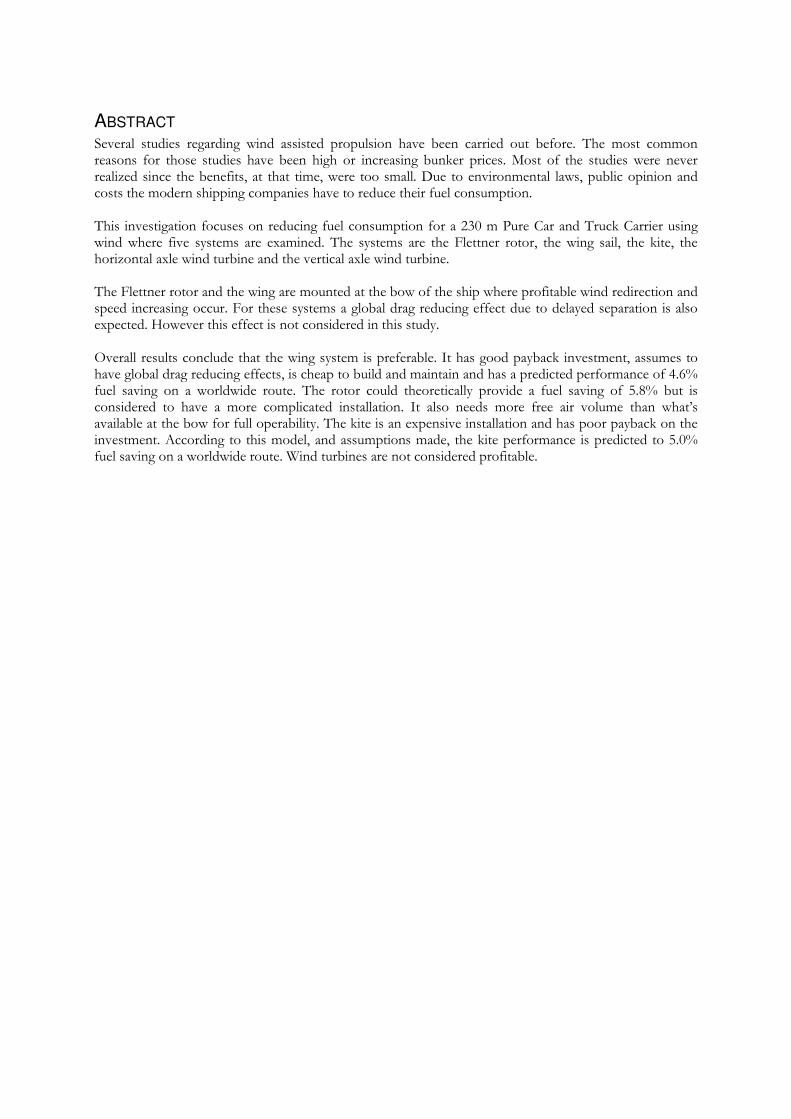
1. INTRODUCTION The world oil price affects the shipping industry costs and profits. The current environmental awareness also makes it more urgent to reduce the consumption of fossil fuel. This master thesis will focus on how to reduce costs and pollution by using wind as a power source for ships. During the analysis Wallenius Marine AB is the assigner and the Pure Car Truck Carrier (PCTC) Fedora will serve as norm. Analyzing different systems will make it possible to decide whether it is profitable or not to install wind powered propulsion. The decisions will be based on a cost benefit analysis which is strictly related to the oil price. It should also be considered that a wind assisted fleet is less sensitive to oil price fluctuations. The International Energy Agency, IEA, states in the report World Energy Outlook 2008 that the oil price will increase to over 100 $/barrel when the world economy has stabilized. By the year of 2030 the oil price claims to have increased above 200 $/barrel [IEA, 2008]. Figure 1 presents the oil price development from 2004 to 2009. This study started when oil price was at its peak.

Figure 1, Oil price development $/barrel, Platts Brent intra index [E24, 2009].

1.1. OBJECTIVE

The history reveals many different methods and ideas for wind propulsion, and several studies in how to gain sail power for merchant vessels have been done before. This investigation will initially consider earlier investigations performed. Based on the outcome from this analysis interesting systems will be further analyzed. The study will focus on the best performing and feasible systems for different types of wind auxiliary propulsion. A comparison will tell which of the systems that could be profitable and useful on a ship in the Wallenius fleet. It is desired that the considered systems can be retrofitted without changing the ship design drastically, for example high masts can give trouble with heeling and passing bridges. The performance of the systems will be predicted using wind statistics from relevant routes.

1.2. METHOD

By using basic ship theory and fluid dynamics a Power Prediction Program (PPP) is developed and utilized to predict the performance of the different systems. Some of the data that are used as input to the PPP are collected from previous wind tunnel tests and towing tank tests of the PCTC Fedora. Others are calculated using ship data and semi empirical approximations. The calculations are performed in Matlab from The Mathworks Inc. which can handle the extensive model. A minor two dimensional fluid dynamical analysis is performed in Fluent from Fluent Inc. Relevant wind statistics are retrieved from the European Center for Medium-range Weather Forecasts, (ECMWF) data.

1.3. STUDIED SYSTEMS

Four different techniques for utilizing wind will be analyzed in this report and they are briefly introduced here.

1.3.1. The Flettner Rotor

The technique of a spinning rotor using the Magnus effect was tried on a ship as early as in 1924, but was never considered to be a good alternative since the oil price was so low and the profits were small. But the

9

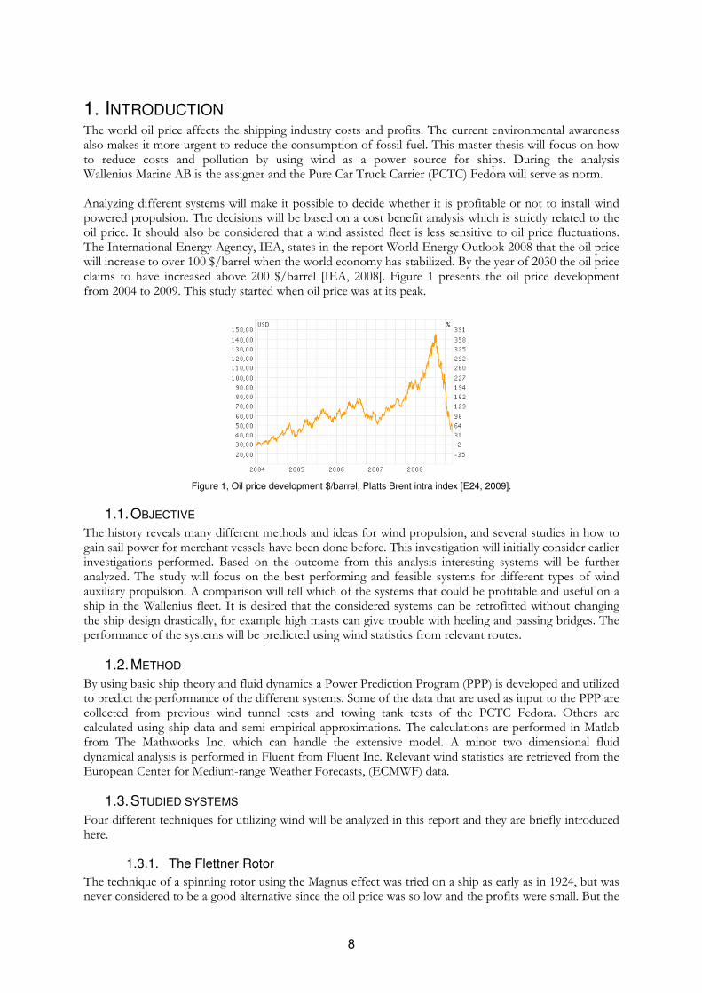
shipping industry have reconsidered this and the wind mill building company Enercon is at the moment constructing a ship with auxiliary propulsion of 4 large Flettner rotors of 25 meters height, see Figure 2 [Enercon, 2008].

Figure 2, The E-ship ordered by Enercon is a 130 m freighter that will be equipped with four 24m high rotors that uses the

Magnus effect. It will be finished in 2009 [Enercon, 2008].

1.3.2. The kite

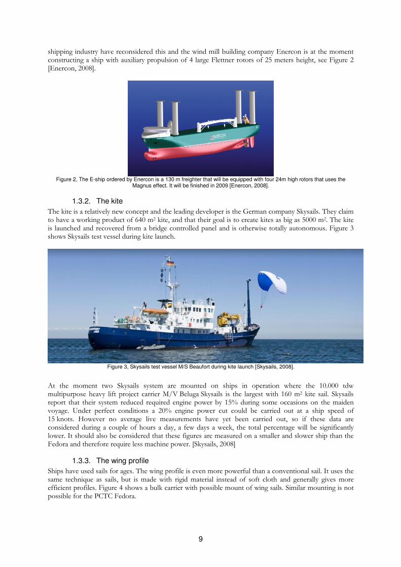
The kite is a relatively new concept and the leading developer is the German company Skysails. They claim to have a working product of 640 m2 kite, and that their goal is to create kites as big as 5000 m2. The kite is launched and recovered from a bridge controlled panel and is otherwise totally autonomous. Figure 3 shows Skysails test vessel during kite launch.

Figure 3, Skysails test vessel M/S Beaufort during kite launch [Skysails, 2008].

At the moment two Skysails system are mounted on ships in operation where the 10.000 tdw multipurpose heavy lift project carrier M/V Beluga Skysails is the largest with 160 m2 kite sail. Skysails report that their system reduced required engine power by 15% during some occasions on the maiden voyage. Under perfect conditions a 20% engine power cut could be carried out at a ship speed of 15 knots. However no average live measurements have yet been carried out, so if these data are considered during a couple of hours a day, a few days a week, the total percentage will be significantly lower. It should also be considered that these figures are measured on a smaller and slower ship than the Fedora and therefore require less machine power. [Skysails, 2008]

1.3.3. The wing profile

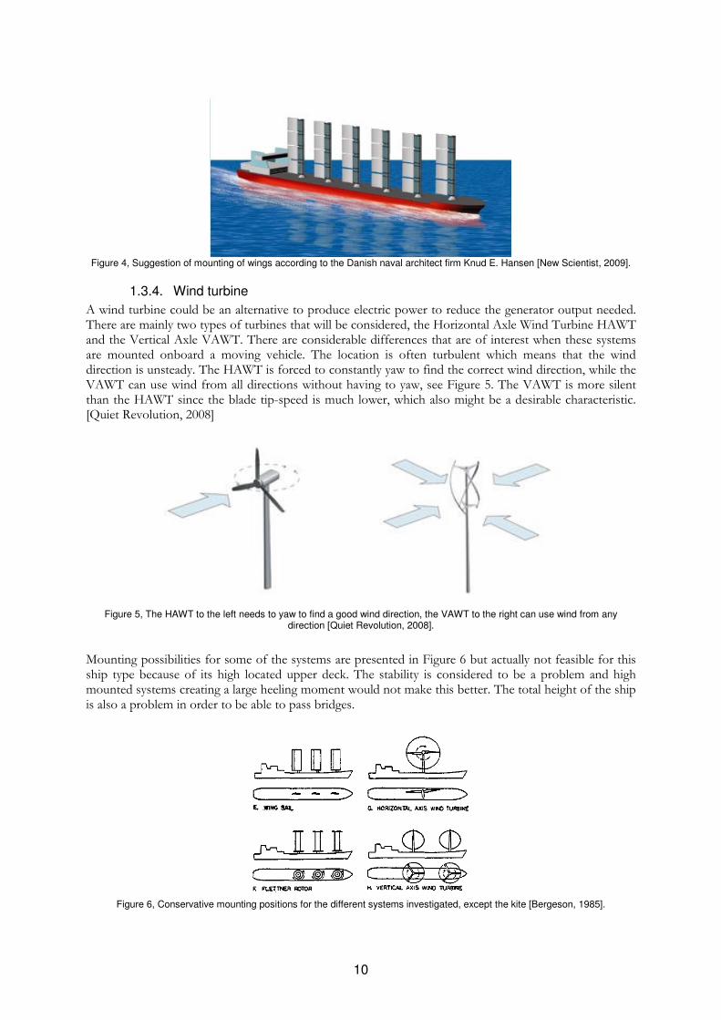
Ships have used sails for ages. The wing profile is even more powerful than a conventional sail. It uses the same technique as sails, but is made with rigid material instead of soft cloth and generally gives more efficient profiles. Figure 4 shows a bulk carrier with possible mount of wing sails. Similar mounting is not possible for the PCTC Fedora.

10

Figure 4, Suggestion of mounting of wings according to the Danish naval architect firm Knud E. Hansen [New Scientist, 2009].

1.3.4. Wind turbine

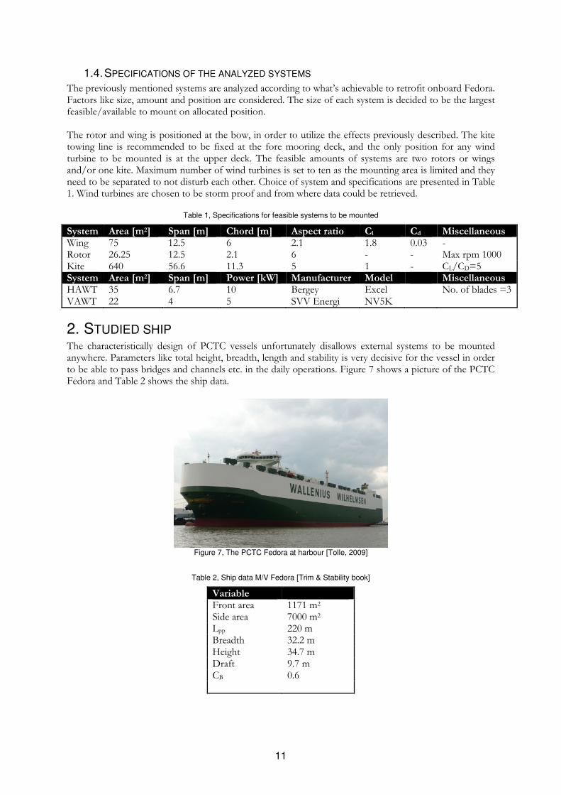
A wind turbine could be an alternative to produce electric power to reduce the generator output needed. There are mainly two types of turbines that will be considered, the Horizontal Axle Wind Turbine HAWT and the Vertical Axle VAWT. There are considerable differences that are of interest when these systems are mounted onboard a moving vehicle. The location is often turbulent which means that the wind direction is unsteady. The HAWT is forced to constantly yaw to find the correct wind direction, while the VAWT can use wind from all directions without having to yaw, see Figure 5. The VAWT is more silent than the HAWT since the blade tip-speed is much lower, which also might be a desirable characteristic. [Quiet Revolution, 2008]

Figure 5, The HAWT to the left needs to yaw to find a good wind direction, the VAWT to the right can use wind from any

direction [Quiet Revolution, 2008].

Mounting possibilities for some of the systems are presented in Figure 6 but actually not feasible for this ship type because of its high located upper deck. The stability is considered to be a problem and high mounted systems creating a large heeling moment would not make this better. The total height of the ship is also a problem in order to be able to pass bridges.

Figure 6, Conservative mounting positions for the different systems investigated, except the kite [Bergeson, 1985].

11

1.4. SPECIFICATIONS OF THE ANALYZED SYSTEMS

The previously mentioned systems are analyzed according to what’s achievable to retrofit onboard Fedora. Factors like size, amount and position are considered. The size of each system is decided to be the largest feasible/available to mount on allocated position. The rotor and wing is positioned at the bow, in order to utilize the effects previously described. The kite towing line is recommended to be fixed at the fore mooring deck, and the only position for any wind turbine to be mounted is at the upper deck. The feasible amounts of systems are two rotors or wings and/or one kite. Maximum number of wind turbines is set to ten as the mounting area is limited and they need to be separated to not disturb each other. Choice of system and specifications are presented in Table 1. Wind turbines are chosen to be storm proof and from where data could be retrieved.

Table 1, Specifications for feasible systems to be mounted

System Area [m2] Span [m] Chord [m] Aspect ratio Cl Cd Miscellaneous Wing 75 12.5 6 2.1 1.8 0.03 - Rotor 26.25 12.5 2.1 6 - - Max rpm 1000 Kite 640 56.6 11.3 5 1 - CL/CD=5 System Area [m2] Span [m] Power [kW] Manufacturer Model Miscellaneous HAWT 35 6.7 10 Bergey Excel No. of blades =3 VAWT 22 4 5 SVV Energi NV5K

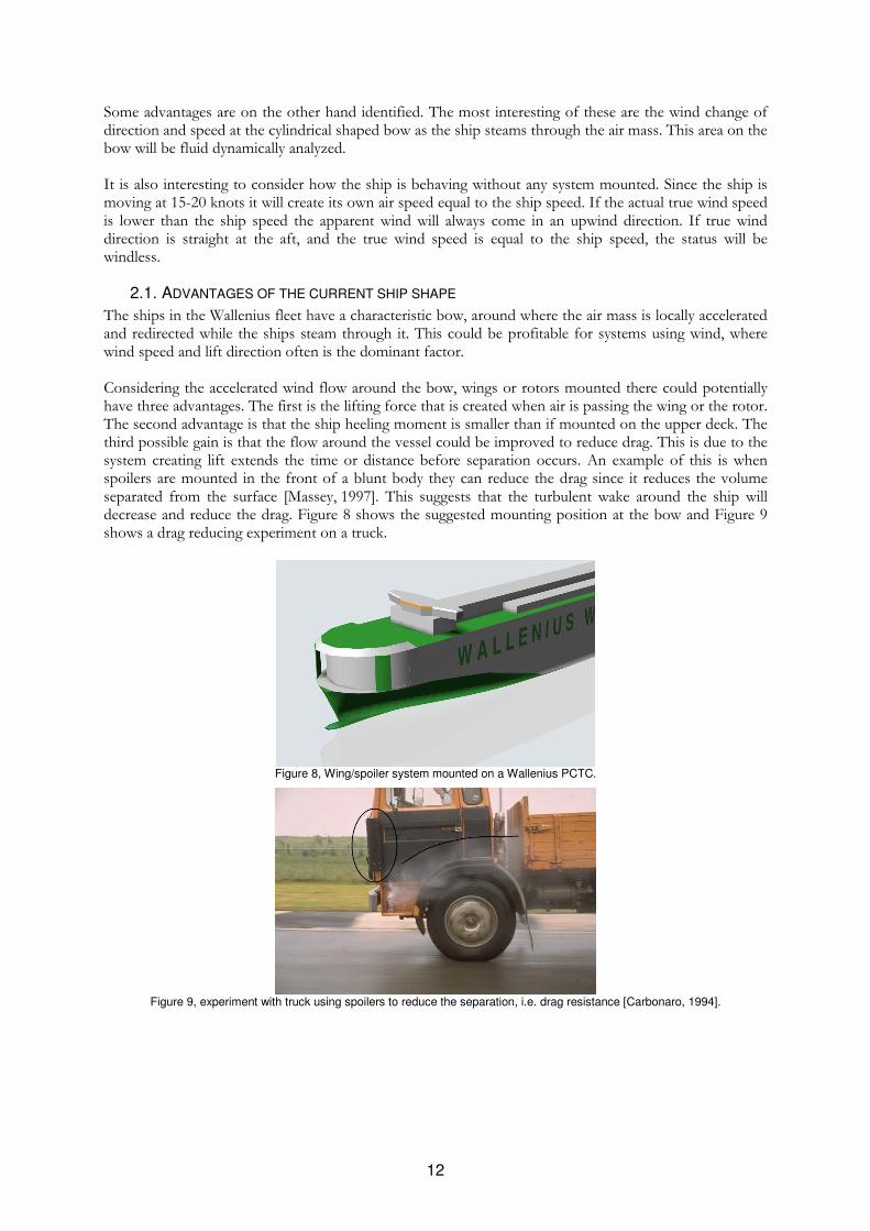
2. STUDIED SHIP The characteristically design of PCTC vessels unfortunately disallows external systems to be mounted anywhere. Parameters like total height, breadth, length and stability is very decisive for the vessel in order to be able to pass bridges and channels etc. in the daily operations. Figure 7 shows a picture of the PCTC Fedora and Table 2 shows the ship data.

Figure 7, The PCTC Fedora at harbour [Tolle, 2009]

Table 2, Ship data M/V Fedora [Trim & Stability book]

Variable Front area 1171 m2 Side area 7000 m2 Lpp 220 m Breadth 32.2 m Height 34.7 m Draft 9.7 m CB 0.6

12

Some advantages are on the other hand identified. The most interesting of these are the wind change of direction and speed at the cylindrical shaped bow as the ship steams through the air mass. This area on the bow will be fluid dynamically analyzed. It is also interesting to consider how the ship is behaving without any system mounted. Since the ship is moving at 15-20 knots it will create its own air speed equal to the ship speed. If the actual true wind speed is lower than the ship speed the apparent wind will always come in an upwind direction. If true wind direction is straight at the aft, and the true wind speed is equal to the ship speed, the status will be windless.

2.1. ADVANTAGES OF THE CURRENT SHIP SHAPE

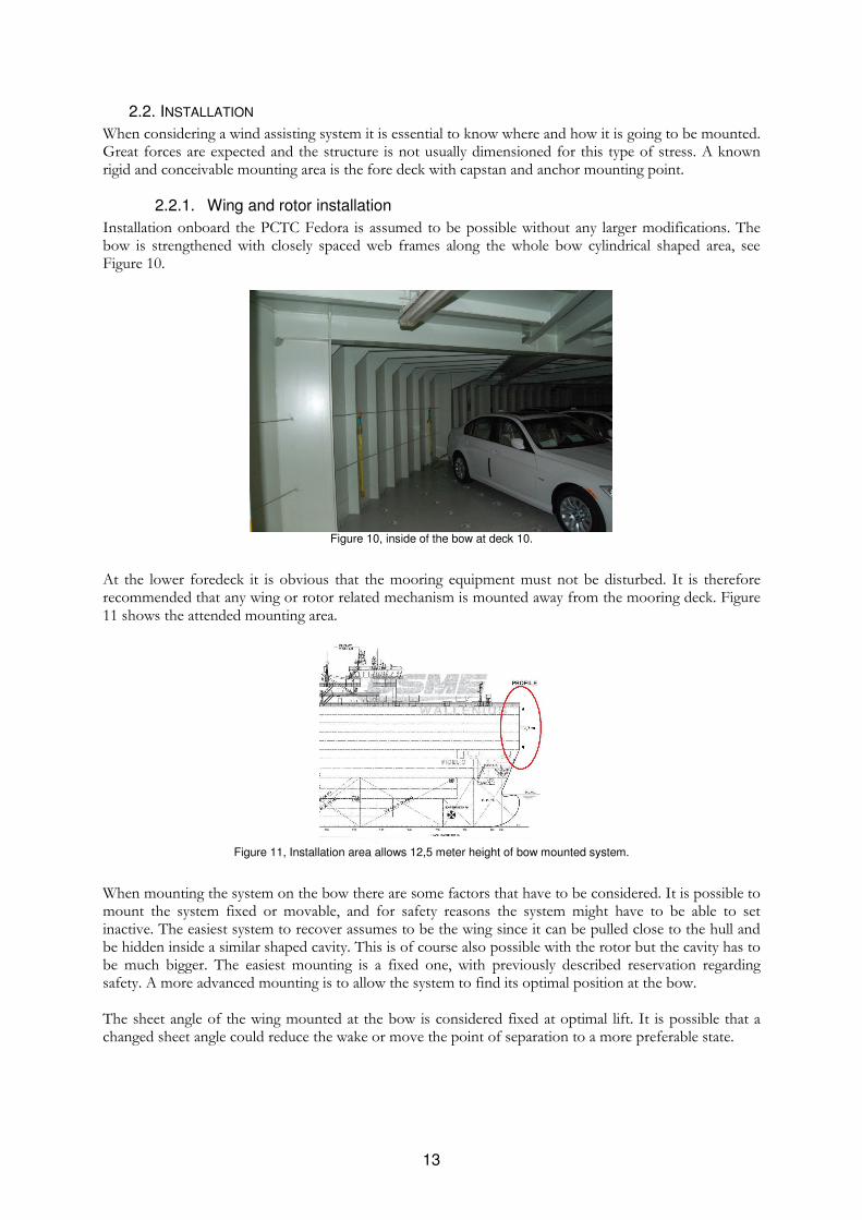
The ships in the Wallenius fleet have a characteristic bow, around where the air mass is locally accelerated and redirected while the ships steam through it. This could be profitable for systems using wind, where wind speed and lift direction often is the dominant factor. Considering the accelerated wind flow around the bow, wings or rotors mounted there could potentially have three advantages. The first is the lifting force that is created when air is passing the wing or the rotor. The second advantage is that the ship heeling moment is smaller than if mounted on the upper deck. The third possible gain is that the flow around the vessel could be improved to reduce drag. This is due to the system creating lift extends the time or distance before separation occurs. An example of this is when spoilers are mounted in the front of a blunt body they can reduce the drag since it reduces the volume separated from the surface [Massey, 1997]. This suggests that the turbulent wake around the ship will decrease and reduce the drag. Figure 8 shows the suggested mounting position at the bow and Figure 9 shows a drag reducing experiment on a truck.

Figure 8, Wing/spoiler system mounted on a Wallenius PCTC.

Figure 9, experiment with truck using spoilers to reduce the separation, i.e. drag resistance [Carbonaro, 1994].

13

2.2. INSTALLATION

When considering a wind assisting system it is essential to know where and how it is going to be mounted. Great forces are expected and the structure is not usually dimensioned for this type of stress. A known rigid and conceivable mounting area is the fore deck with capstan and anchor mounting point.

2.2.1. Wing and rotor installation

Installation onboard the PCTC Fedora is assumed to be possible without any larger modifications. The bow is strengthened with closely spaced web frames along the whole bow cylindrical shaped area, see Figure 10.

Figure 10, inside of the bow at deck 10.

At the lower foredeck it is obvious that the mooring equipment must not be disturbed. It is therefore recommended that any wing or rotor related mechanism is mounted away from the mooring deck. Figure 11 shows the attended mounting area.

Figure 11, Installation area allows 12,5 meter height of bow mounted system.

When mounting the system on the bow there are some factors that have to be considered. It is possible to mount the system fixed or movable, and for safety reasons the system might have to be able to set inactive. The easiest system to recover assumes to be the wing since it can be pulled close to the hull and be hidden inside a similar shaped cavity. This is of course also possible with the rotor but the cavity has to be much bigger. The easiest mounting is a fixed one, with previously described reservation regarding safety. A more advanced mounting is to allow the system to find its optimal position at the bow. The sheet angle of the wing mounted at the bow is considered fixed at optimal lift. It is possible that a changed sheet angle could reduce the wake or move the point of separation to a more preferable state.

14

2.2.2. Kite installation

The kite has a recovery and launch module called SkySails Arrangement Module, SAM, and a winch. The winch is where the towing line is fixed. It is assumed that the winch can be mounted away from the SAM in order to decrease the heeling produced. On Fedora the winch could be mounted below the mooring deck by the bosun storage compartment, and the SAM can be mounted up on the forecastle. This would create a smaller heeling momentum than if the winch also would be mounted on the forecastle. In previous calculations, mainly considering heeling tank volume, the winch mounting position is at the mooring deck. It is considered better to mount the winch close to the mooring deck since it is dimensioned for great strains due to the reinforcements around the capstan and anchor windlass.

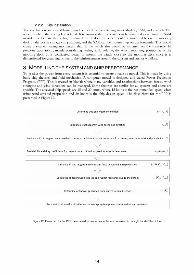
3. MODELLING THE SYSTEM AND SHIP PERFORMANCE To predict the power from every system it is essential to create a realistic model. This is made by using basic ship theories and fluid mechanics. A computer model is designed and called Power Prediction Program, (PPP). This is created in Matlab where many variables and relationships between forces, wind strengths and wind directions can be managed. Some theories are similar for all systems and some are specific. The analyzed ship speeds are 15 and 20 knots, where 15 knots is the recommended speed when using wind assisted propulsion and 20 knots is the ship design speed. The flow chart for the PPP is presented in Figure 12.

For a statistical weather distribution the average system power is summarized and evaluated.

Determine net power generated from system in ship direction

Decide the added induced side slip and rudder resistance due to the system

Calculate lift and drag from system, and force generated in ship direction

Establish lift and drag coefficients for present system. Rotation speed for rotor is determined

Decide total ship engine power needed at current condition. Consider resistance from waves, wind induced side slip and wind

Calculate actual apparent wind speed and direction

Determine ship and weather condition ( ), ,T SV V γ

( ),AV β

( )P

( , , )L D rot

C C U

( ), , ,S SxA yA

L D F F

( )S

P

( ),HS RxA xH

F F

Figure 12, Flow chart for the PPP, determined or needed variables are presented in the right hand of the picture

15

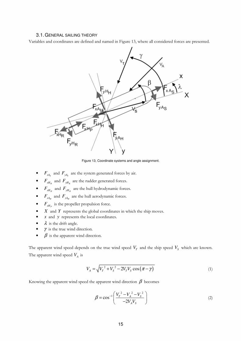
3.1. GENERAL SAILING THEORY

Variables and coordinates are defined and named in Figure 13, where all considered forces are presented.

Figure 13, Coordinate systems and angle assignment.

• SxA

F and SyA

F are the system generated forces by air.

• RxH

F and RyH

F are the rudder generated forces.

• HxH

F and HyH

F are the hull hydrodynamic forces.

• HxA

F and HyA

F are the hull aerodynamic forces.

• PxH

F is the propeller propulsion force.

• X and Y represents the global coordinates in which the ship moves.

• x and y represents the local coordinates.

• λ is the drift angle.

• γ is the true wind direction.

• β is the apparent wind direction.

The apparent wind speed depends on the true wind speed TV and the ship speed SV which are known.

The apparent wind speed A

V is

( )2 22 cosA T S T SV V V V V π γ= + − − (1)

Knowing the apparent wind speed the apparent wind direction β becomes

2 2 2

1cos2

T A S

A S

V V V

V Vβ − − −

= −

(2)

16

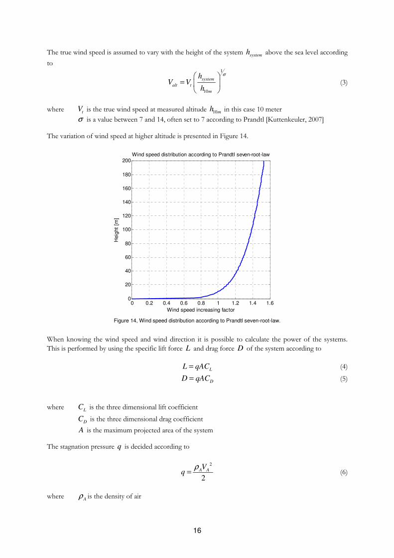
The true wind speed is assumed to vary with the height of the system system

h above the sea level according

to

1

10

system

alt t

m

hV V

h

σ =

(3)

where tV is the true wind speed at measured altitude 10mh in this case 10 meter

σ is a value between 7 and 14, often set to 7 according to Prandtl [Kuttenkeuler, 2007] The variation of wind speed at higher altitude is presented in Figure 14.

0 0.2 0.4 0.6 0.8 1 1.2 1.4 1.60

20

40

60

80

100

120

140

160

180

200Wind speed distribution according to Prandtl seven-root-law

Heig

ht

[m]

Wind speed increasing factor

Figure 14, Wind speed distribution according to Prandtl seven-root-law.

When knowing the wind speed and wind direction it is possible to calculate the power of the systems.

This is performed by using the specific lift force L and drag force D of the system according to

L

L qAC= (4)

DD qAC= (5)

where L

C is the three dimensional lift coefficient

DC is the three dimensional drag coefficient

A is the maximum projected area of the system The stagnation pressure q is decided according to

2

2

A AV

qρ

= (6)

where A

ρ is the density of air

17

Note that L

C and D

C is different for every system and decided in the System specific chapter.

Translation is thereafter made to determine the effective force in the ship moving direction xF and the

orthogonal side force y

F . The translation is performed by using the Euler rotation theorem according to

cos sin

sin cos

S

S

xA

yA

F D

F L

β β

β β

− = −

(7)

3.2. TOTAL ENGINE POWER NEEDED

The effective engine power needed at no wind is 4900 kW at 15 knots and 12000 kW at 20 knots. When true wind is present additional engine power is needed. The superstructure of the vessel will cause a large

force due to the apparent wind both in y-direction HyAF and x-direction

HxAF . The force in the y-

direction will induce side slip and heel the vessel, however the heeling generated from the superstructure is not considered. The force in x-direction on the ship hull will either reduce or increase the required engine

power. The following calculation is based on wind drag coefficients xC and yC determined in wind

tunnel tests performed on a model of M/V Fedora by DSME at Force Technology in Denmark.

21

2HxA A A F xF V A Cρ= (8)

21

2HyA A A S yF V A Cρ= (9)

where F

A is the frontal area of the ship

S

A is the side area of the ship

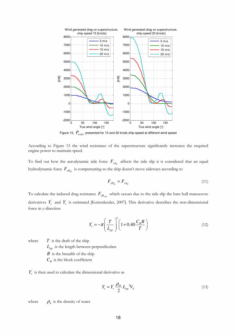
The calculated equivalent engine power wind

P needed due to the wind drag are presented in Figure 15

according to

HxA S

wind

ship

F VP

η

⋅= (10)

18

0 50 100 150-2000

-1000

0

1000

2000

3000

4000

5000

6000

7000

8000

Wind generated drag on superstructure, ship speed 15 [knots]

[kW

]

True wind angle [°]

0 50 100 150-2000

-1000

0

1000

2000

3000

4000

5000

6000

7000

8000

Wind generated drag on superstructure, ship speed 20 [knots]

[kW

]


5 m/s

10 m/s

15 m/s

20 m/s

5 m/s

10 m/s

15 m/s

20 m/s

Figure 15,

windP presented for 15 and 20 knots ship speed at different wind speed

According to Figure 15 the wind resistance of the superstructure significantly increases the required engine power to maintain speed.

To find out how the aerodynamic side force HyA

F affects the side slip it is considered that an equal

hydrodynamic force HyH

F is compensating so the ship doesn’t move sideways according to

H HyH yA

F F= (11)

To calculate the induced drag resistance slipxH

F which occurs due to the side slip the bare hull manoeuvre

derivatives '

vY and

vY is estimated [Kuttenkeuler, 2007]. This derivative describes the non-dimensional

force in y-direction

2

' 1 0.40 Bv

pp

C BTY

L Tπ

= − + (12)

where T is the draft of the ship

ppL is the length between perpendiculars

B is the breadth of the ship

B

C is the block coefficient

'

vY is then used to calculate the dimensional derivative as

' 2

2

Hv v pp S

Y Y L Vρ

= (13)

where h

ρ is the density of water

19

The force in the y-direction is speed dependent and the leeway angle λ is calculated.

1tan tan H

H

yH

yH v S

S v

FF Y V

V Yλ λ −

= ⇔ =

(14)

Knowing the leeway angle λ it is possible to estimate the expected side slip resistance slipxHF . This

resistance will reduce the system’s ability to save fuel since the ship has to yaw to keep course. The drift

resistance slipxHF is according to [Schentzle, 1985] calculated as

2

22 2

1

1

1slip H

DCxH yH

pp

h S

kF F

k LV k T

k Tρ λ

= −

+

(15)

where DCk ≈ 1 - 1.2

1k ≈ 2

2k ≈ 0.2 – 0.3

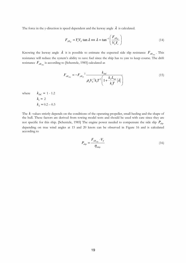
The k -values strictly depends on the conditions of the operating propeller, small heeling and the shape of the hull. These factors are derived from towing model tests and should be used with care since they are

not specific for this ship. [Schentzle, 1985] The engine power needed to compensate the side slip slipP

depending on true wind angles at 15 and 20 knots can be observed in Figure 16 and is calculated according to

slipxH S

slip

ship

F VP

η

⋅= (16)

20

0 50 100 150 2000

2000

4000

6000

8000

Wind generated drift resistance,

ship speed 15 [knots]

[kW

]


0 50 100 1500

5

10

15

Leeway angle λ due to true wind, ship speed 15 [knots]

Leew

ay a

ngle

λ [

°]


0 50 100 150 2000

2000

4000

6000

8000

Wind generated drift resistance,


[kW

]


0 50 100 1500

5

10

15

Leeway angle λ due to true wind, ship speed 20 [knots]

Leew

ay a

ngle

λ [

°]True wind angle [°]

5 m/s

10 m/s

15 m/s

20 m/s

Figure 16, The engine power needed to compensate the side slip slipP and leeway angle λ for 15 and 20 knots ship speed at

different true wind speed and wind angles.

Notice that quite large compensation has to be made due to side slip. Additional engine power needed is similar for 15 and 20 knots, but leeway angles are almost twice as big at 15 knots. The conclusion is that lower speed needs higher leeway angle to compensate. The magnitude of theses leeway angles are confirmed during an interview with the crew members of M/V Undine, a similar ship to M/V Fedora. Added resistance due to waves also increases the engine power needed. Waves are assumed to have the same direction as the true wind angle. Assuming that a certain wind strength correlates to a certain sea state, using the Beaufort table, the wave added resistance is roughly approximated based on Wallenius

Marine model data. Approximated increase of power waveP is presented in Figure 17.

0 50 100 1500

2000

4000

6000

8000

10000

12000

Wave generated resistance, ship speed 15 [knots]


Engin

e p

ow

er

[kW

]

0 50 100 1500

2000

4000

6000

8000

10000

12000

Wave generated resistance, ship speed 20 [knots]


Engin

e p

ow

er

[kW

]

5 m/s

10 m/s

15 m/s

20 m/s

Figure 17, Approximated wave induced resistance in equivalent engine power waveP .

21

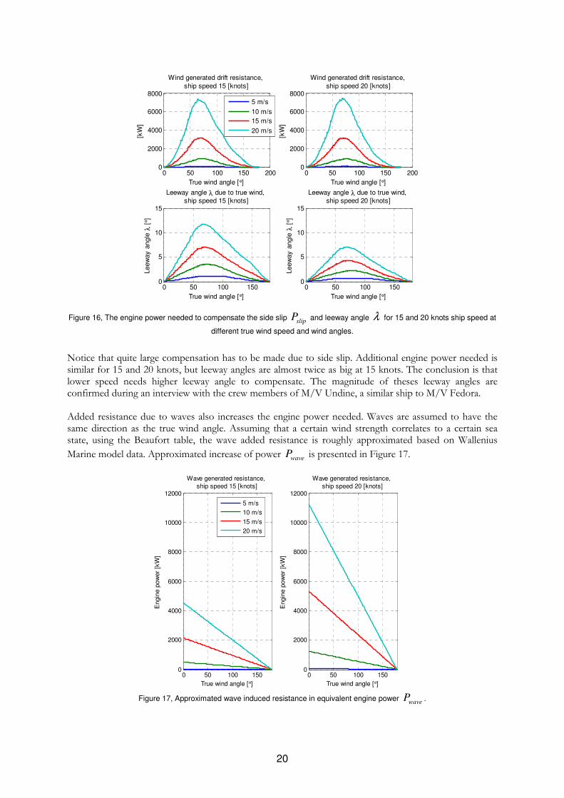
The estimated total induced wave, wind and side slip resistance slip wind waveP P P P= + + is presented in

Figure 18 as equivalent engine power.

0 50 100 1500

5

10

15

20

25

30

Total wind, side slip and wave generated resistance, ship speed 20 [knots]

[MW

]


0 50 100 1500

5

10

15

20

25

30

Total wind, side slip and wave generated resistance, ship speed 15 [knots]

[MW

]


5 m/s

10 m/s

15 m/s

20 m/s

Figure 18, Total engine power required [MW] at 15 and 20 knots ship speed. Wind, side slip and wave generated resistance

included for different true wind speed and wind angle. The black dashed line shows required power at no wind, the red dashed line shows available engine power.

At unfavourable winds it will occasionally be impossible for the ship to keep designated speed due to the high resistance. It can also be seen that the ship already is making profitable sailing at true wind speed above ship speed when wind direction is favourable, this is presented as negative power at true wind angles.

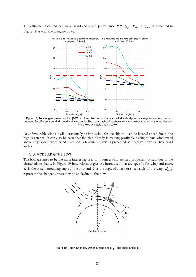
3.3. MODELLING THE BOW

The bow assumes to be the most interesting area to mount a wind assisted propulsion system due to the characteristic shape. In Figure 19 bow related angles are introduced that are specific for wing and rotor.

ζ is the system mounting angle at the bow and δ is the angle of attack or sheet angle of the wing. localβ

represent the changed apparent wind angle due to the bow.

Figure 19, Top view of bow with mounting angle ζ and sheet angle δ .

22

To predict the wind speed magnification at the bow a minor two dimensional CFD analysis is performed. During the analysis the program Fluent is used. Simulating the ship and bow two-dimensional is assumed to be a satisfactory method to approximate how the wind behaves. The method considers friction and bow simulation allows apparent wing angle changes. Laminar flow is used, and the flow for 40 degrees apparent wind angle is shown in Figure 20.

Figure 20, Top view of the starboard side of the bow showing the 2-dimensional flow around the bow at apparent wind direction 40 degrees port from the bow. The scale at the left hand of the picture shows the wind speed magnification. Note the separation

in the upper right corner of the picture.

The results from CFD analysis reveal the magnification of the wind speed and also the interesting point of separation. As seen in Figure 20 separation occurs in the upper right corner, about 50 degrees of the bow. Separation, wakes and turbulence create more total ship drag and it is also an unprofitable area for the wing to create lift. Due to this it is important to place the wing before the separation point for it to be able to create lift and delay the separation. Bow mounted systems are not effective when positioned close to the area of separation. This can be

observed in Figure 21 where magnification is low at high ζ . The cross in the plot marks an example of

mount position on bow ζ = 30 degrees and apparent wind direction β =20 degrees. Wind speed

magnification is about 1.7.

23

10

20

30

40

50

60

70

80

90

10 20 30 40 50 60

ζ Position on bow [°]

β A

ppare

nt

win

d d

irection [

°]

0

0.5

1

1.5

2

2.5

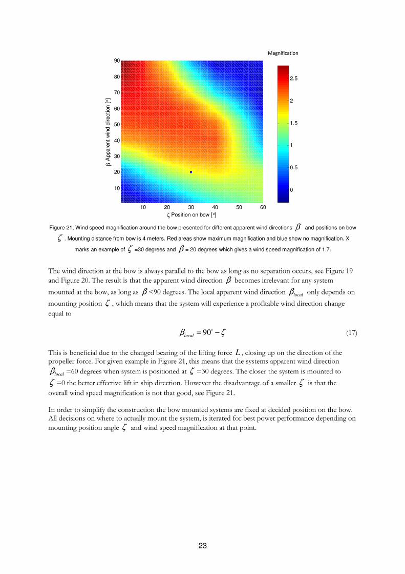
Figure 21, Wind speed magnification around the bow presented for different apparent wind directions β and positions on bow

ζ . Mounting distance from bow is 4 meters. Red areas show maximum magnification and blue show no magnification. X

marks an example of ζ =30 degrees and β = 20 degrees which gives a wind speed magnification of 1.7.

The wind direction at the bow is always parallel to the bow as long as no separation occurs, see Figure 19

and Figure 20. The result is that the apparent wind direction β becomes irrelevant for any system

mounted at the bow, as long as β <90 degrees. The local apparent wind direction localβ only depends on

mounting position ζ , which means that the system will experience a profitable wind direction change

equal to

90localβ ζ= −� (17)

This is beneficial due to the changed bearing of the lifting force L , closing up on the direction of the propeller force. For given example in Figure 21, this means that the systems apparent wind direction

localβ =60 degrees when system is positioned at ζ =30 degrees. The closer the system is mounted to

ζ =0 the better effective lift in ship direction. However the disadvantage of a smaller ζ is that the

overall wind speed magnification is not that good, see Figure 21. In order to simplify the construction the bow mounted systems are fixed at decided position on the bow. All decisions on where to actually mount the system, is iterated for best power performance depending on

mounting position angle ζ and wind speed magnification at that point.

Magnification

24

3.4. SYSTEM SPECIFIC THEORY

Analyzed systems are selected from what is feasible to retrofit onboard the fleet and what is assumed to be generating profitable power. This chapter will describe the power generated from different systems in detail. Most of the power presentations in the following figures are presented in equivalent engine power

where the ship propulsion efficiency shipη is set to 0.75 [DSME, 2007]. System power in ship direction

SP is

SxA S

S

ship

F VP

η

⋅= (18)

The rotor and the wing system have one part mounted on the port side and the other one mounted on the starboard side. When calculating the system power, only one side of the system is assumed active. It is also considered that no heeling from system will occur since it can be compensated with the onboard heeling tanks.

3.4.1. Flettner rotor

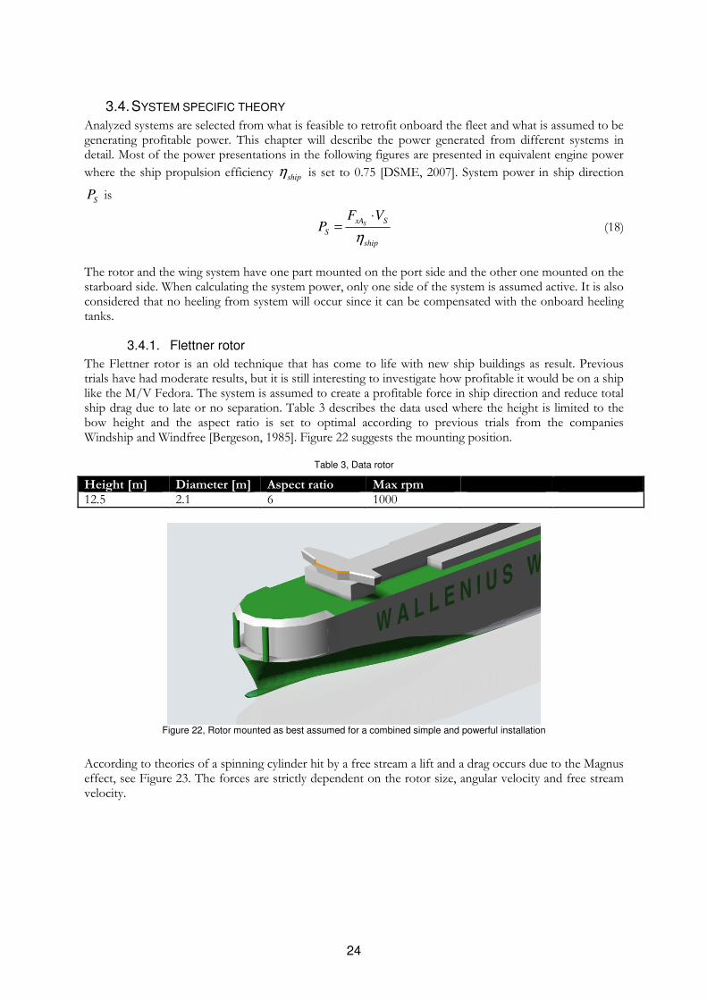
The Flettner rotor is an old technique that has come to life with new ship buildings as result. Previous trials have had moderate results, but it is still interesting to investigate how profitable it would be on a ship like the M/V Fedora. The system is assumed to create a profitable force in ship direction and reduce total ship drag due to late or no separation. Table 3 describes the data used where the height is limited to the bow height and the aspect ratio is set to optimal according to previous trials from the companies Windship and Windfree [Bergeson, 1985]. Figure 22 suggests the mounting position.

Table 3, Data rotor

Height [m] Diameter [m] Aspect ratio Max rpm 12.5 2.1 6 1000

Figure 22, Rotor mounted as best assumed for a combined simple and powerful installation

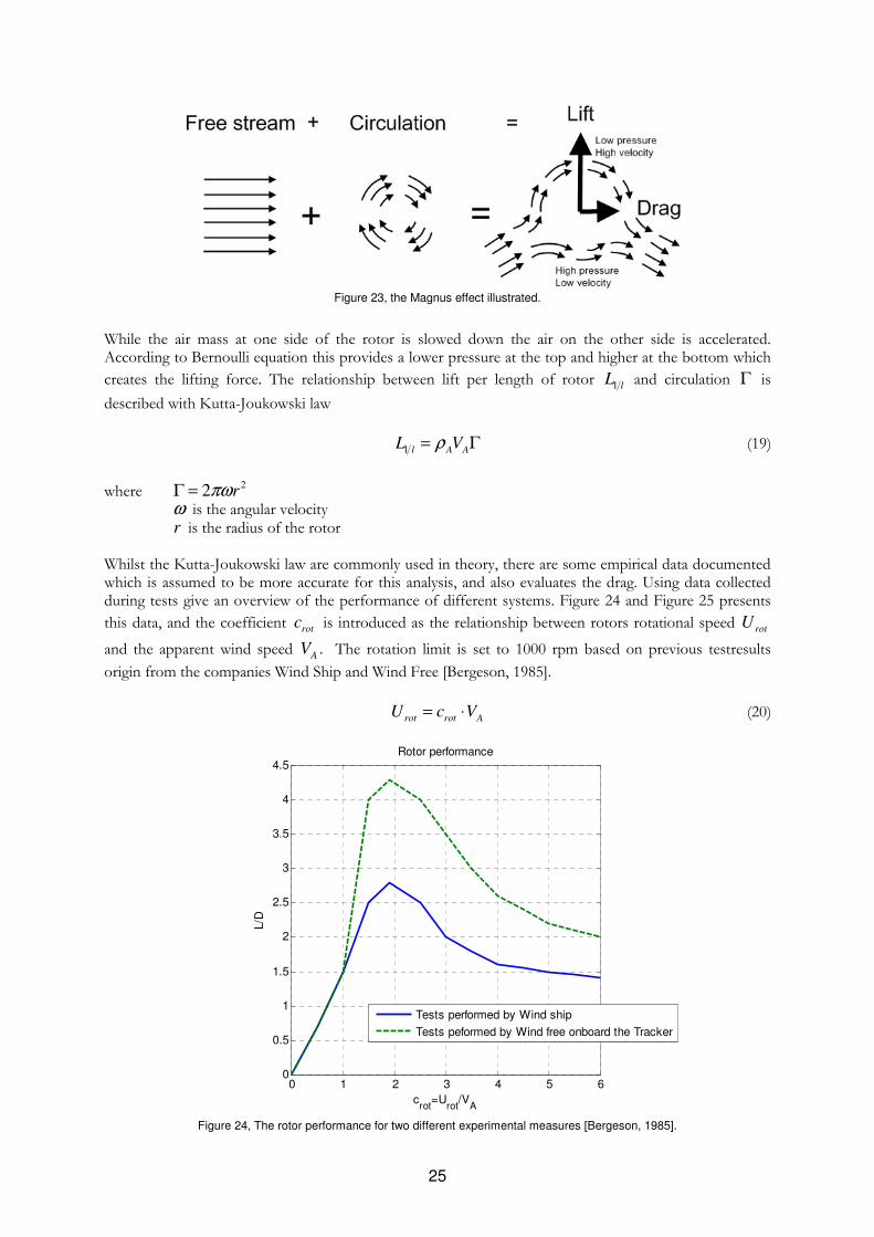
According to theories of a spinning cylinder hit by a free stream a lift and a drag occurs due to the Magnus effect, see Figure 23. The forces are strictly dependent on the rotor size, angular velocity and free stream velocity.

25

Figure 23, the Magnus effect illustrated.

While the air mass at one side of the rotor is slowed down the air on the other side is accelerated. According to Bernoulli equation this provides a lower pressure at the top and higher at the bottom which

creates the lifting force. The relationship between lift per length of rotor 1 lL and circulation Γ is

described with Kutta-Joukowski law

1 l A AL Vρ= Γ (19)

where 22 rπωΓ =

ω is the angular velocity r is the radius of the rotor

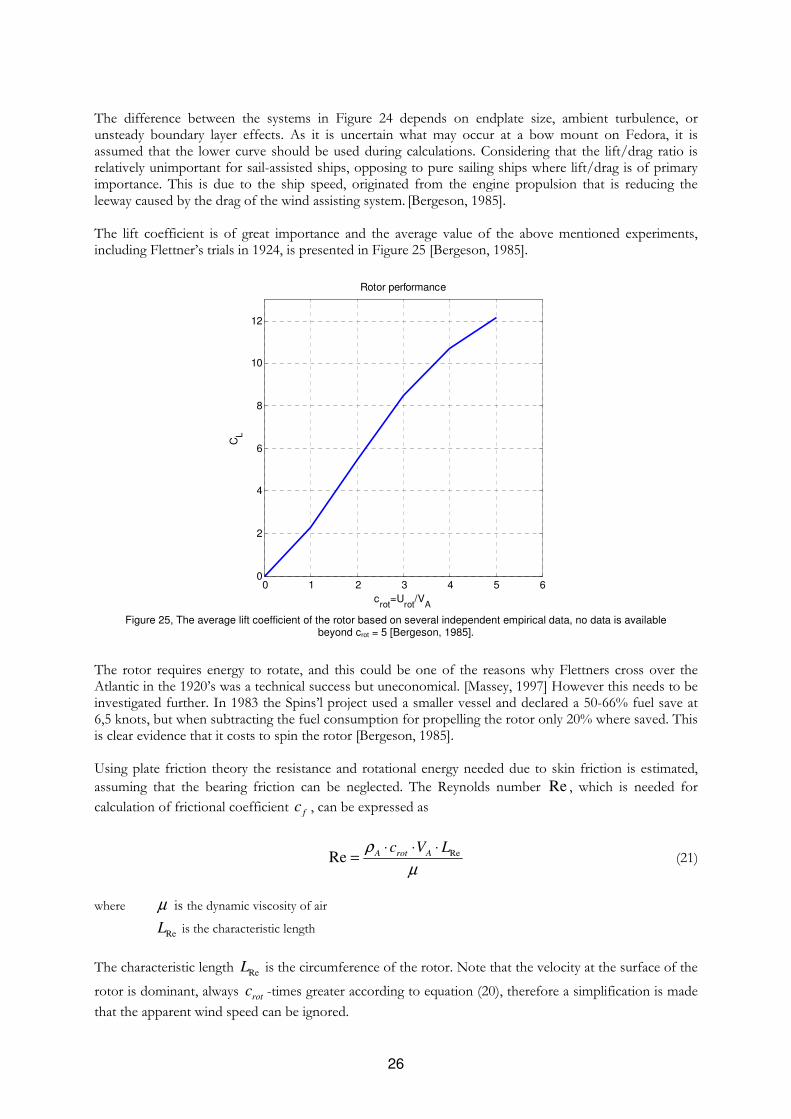
Whilst the Kutta-Joukowski law are commonly used in theory, there are some empirical data documented which is assumed to be more accurate for this analysis, and also evaluates the drag. Using data collected during tests give an overview of the performance of different systems. Figure 24 and Figure 25 presents

this data, and the coefficient rotc is introduced as the relationship between rotors rotational speed rotU

and the apparent wind speed AV . The rotation limit is set to 1000 rpm based on previous testresults

origin from the companies Wind Ship and Wind Free [Bergeson, 1985].

rot rot AU c V= ⋅ (20)

0 1 2 3 4 5 60

0.5

1

1.5

2

2.5

3

3.5

4

4.5

crot

=Urot

/VA

L/D

Rotor performance

Tests performed by Wind ship

Tests peformed by Wind free onboard the Tracker

Figure 24, The rotor performance for two different experimental measures [Bergeson, 1985].

26

The difference between the systems in Figure 24 depends on endplate size, ambient turbulence, or unsteady boundary layer effects. As it is uncertain what may occur at a bow mount on Fedora, it is assumed that the lower curve should be used during calculations. Considering that the lift/drag ratio is relatively unimportant for sail-assisted ships, opposing to pure sailing ships where lift/drag is of primary importance. This is due to the ship speed, originated from the engine propulsion that is reducing the leeway caused by the drag of the wind assisting system. [Bergeson, 1985]. The lift coefficient is of great importance and the average value of the above mentioned experiments, including Flettner’s trials in 1924, is presented in Figure 25 [Bergeson, 1985].

0 1 2 3 4 5 60

2

4

6

8

10

12

crot

=Urot

/VA

CL

Rotor performance

Figure 25, The average lift coefficient of the rotor based on several independent empirical data, no data is available

beyond crot = 5 [Bergeson, 1985].

The rotor requires energy to rotate, and this could be one of the reasons why Flettners cross over the Atlantic in the 1920’s was a technical success but uneconomical. [Massey, 1997] However this needs to be investigated further. In 1983 the Spins’l project used a smaller vessel and declared a 50-66% fuel save at 6,5 knots, but when subtracting the fuel consumption for propelling the rotor only 20% where saved. This is clear evidence that it costs to spin the rotor [Bergeson, 1985]. Using plate friction theory the resistance and rotational energy needed due to skin friction is estimated,

assuming that the bearing friction can be neglected. The Reynolds number Re , which is needed for

calculation of frictional coefficient fc , can be expressed as

ReRe A rot Ac V Lρ

µ

⋅ ⋅ ⋅= (21)

where µ is the dynamic viscosity of air

ReL is the characteristic length

The characteristic length ReL is the circumference of the rotor. Note that the velocity at the surface of the

rotor is dominant, always rotc -times greater according to equation (20), therefore a simplification is made

that the apparent wind speed can be ignored.

27

When Reynolds number is known the frictional coefficient fc is calculated. Equation (22) is valid at both

laminar and turbulent boundary layer as well as high and low Re . [Oklahoma state university, 2008]

2.58

0.455 1700

log(Re) Refc = − (22)

To calculate the total power needed to rotate the rotor the frictional force fF is needed

2

2

rotf f A r

UF c Aρ= (23)

where rA is the surface area of the rotor

The power needed to rotate the rotor revP is hereafter calculated

rev f rotP F U= ⋅ (24)

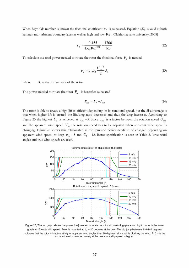
The rotor is able to create a high lift coefficient depending on its rotational speed, but the disadvantage is that when higher lift is created the lift/drag ratio decreases and thus the drag increases. According to

Figure 25 the highest LC is achieved at rotc =5. Since rotc is a factor between the rotation speed rotU

and the apparent wind speed AV , the rotation speed has to be adjusted when apparent wind speed is

changing. Figure 26 shows this relationship as the rpm and power needs to be changed depending on

apparent wind speed, to keep rotc =5 and LC =12. Rotor specification is seen in Table 3. True wind

angles and true wind speeds are used.

0 20 40 60 80 100 120 140 160 1800

50

100

150

200Power to rotate rotor, at ship speed 15 [knots]


[kW

]

5 m/s

10 m/s

15 m/s

20 m/s

0 20 40 60 80 100 120 140 160 1800

500

1000

1500Rotation of rotor, at ship speed 15 [knots]


rpm

5 m/s

10 m/s

15 m/s

20 m/s

Figure 26, The top graph shows the power [kW] needed to rotate the rotor at correlating rpm according to curve in the lower

graph at 15 knots ship speed. Rotor is mounted at ζ = 20 degrees at the bow. The big jump between 110-140 degrees

indicates that the rotor is inactive at higher apparent wind angles than 90 degrees, since hull is blocking the wind. At 5 m/s the apparent wind is always coming at the bow since ship speed is higher.

28

The total power of the system SS xA S revP F V P= ⋅ − is reduced with up to 160 kW due to the cost of

rotating the cylinder, as can be seen in Figure 26. SxAF is calculated according to equation (7) with L and

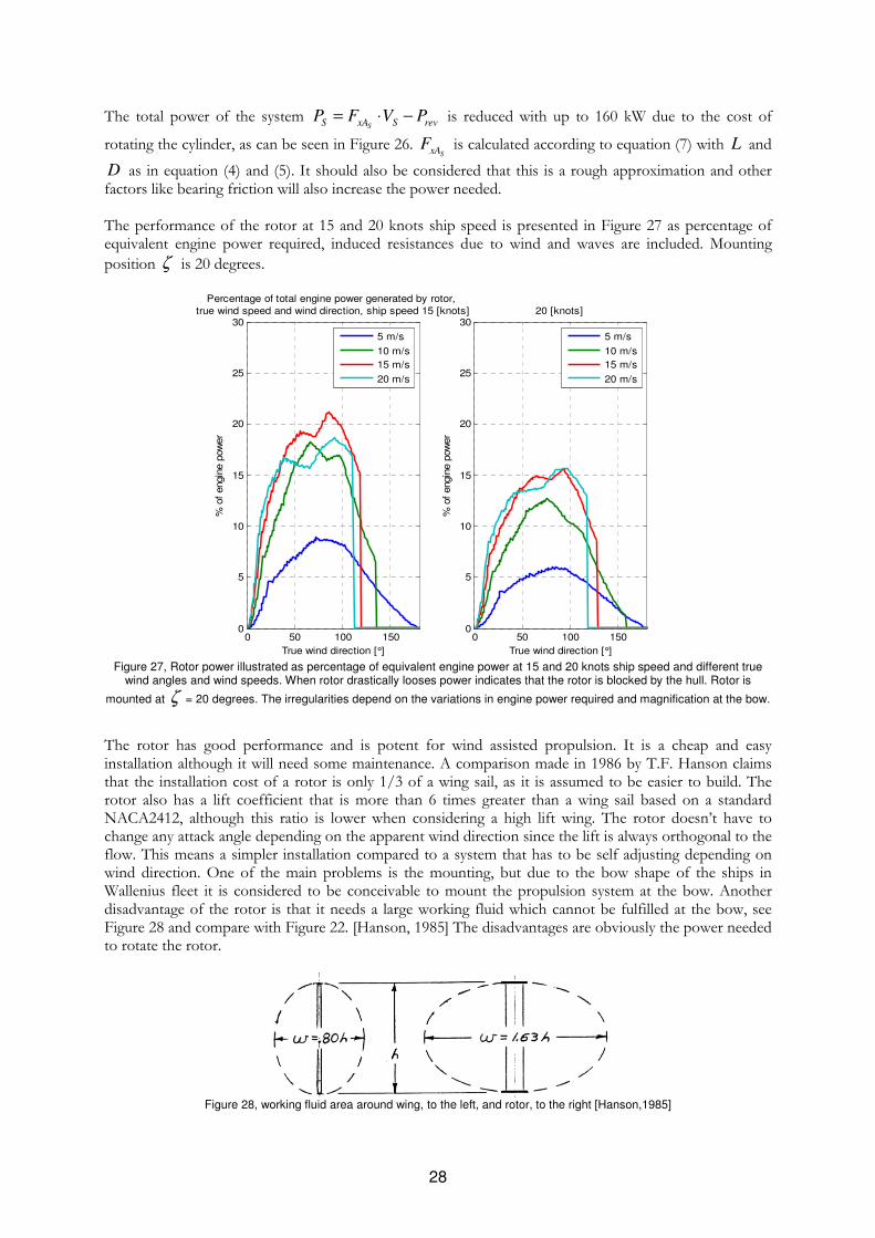
D as in equation (4) and (5). It should also be considered that this is a rough approximation and other factors like bearing friction will also increase the power needed. The performance of the rotor at 15 and 20 knots ship speed is presented in Figure 27 as percentage of equivalent engine power required, induced resistances due to wind and waves are included. Mounting

position ζ is 20 degrees.

0 50 100 1500

5

10

15

20

25

30

True wind direction [°]

% o

f engin

e p

ow

er

Percentage of total engine power generated by rotor,

true wind speed and wind direction, ship speed 15 [knots]

5 m/s

10 m/s

15 m/s

20 m/s

0 50 100 1500

5

10

15

20

25

30


% o

f engin

e p

ow

er

20 [knots]

5 m/s

10 m/s

15 m/s

20 m/s

Figure 27, Rotor power illustrated as percentage of equivalent engine power at 15 and 20 knots ship speed and different true

wind angles and wind speeds. When rotor drastically looses power indicates that the rotor is blocked by the hull. Rotor is

mounted at ζ = 20 degrees. The irregularities depend on the variations in engine power required and magnification at the bow.

The rotor has good performance and is potent for wind assisted propulsion. It is a cheap and easy installation although it will need some maintenance. A comparison made in 1986 by T.F. Hanson claims that the installation cost of a rotor is only 1/3 of a wing sail, as it is assumed to be easier to build. The rotor also has a lift coefficient that is more than 6 times greater than a wing sail based on a standard NACA2412, although this ratio is lower when considering a high lift wing. The rotor doesn’t have to change any attack angle depending on the apparent wind direction since the lift is always orthogonal to the flow. This means a simpler installation compared to a system that has to be self adjusting depending on wind direction. One of the main problems is the mounting, but due to the bow shape of the ships in Wallenius fleet it is considered to be conceivable to mount the propulsion system at the bow. Another disadvantage of the rotor is that it needs a large working fluid which cannot be fulfilled at the bow, see Figure 28 and compare with Figure 22. [Hanson, 1985] The disadvantages are obviously the power needed to rotate the rotor.

Figure 28, working fluid area around wing, to the left, and rotor, to the right [Hanson,1985]

29

3.4.2. The wing

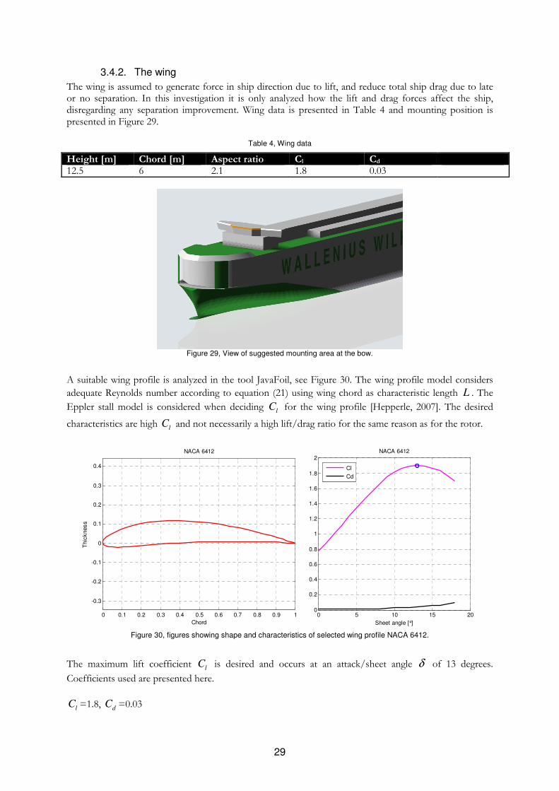
The wing is assumed to generate force in ship direction due to lift, and reduce total ship drag due to late or no separation. In this investigation it is only analyzed how the lift and drag forces affect the ship, disregarding any separation improvement. Wing data is presented in Table 4 and mounting position is presented in Figure 29.

Table 4, Wing data

Height [m] Chord [m] Aspect ratio Cl Cd 12.5 6 2.1 1.8 0.03

Figure 29, View of suggested mounting area at the bow.

A suitable wing profile is analyzed in the tool JavaFoil, see Figure 30. The wing profile model considers

adequate Reynolds number according to equation (21) using wing chord as characteristic length L . The

Eppler stall model is considered when deciding lC for the wing profile [Hepperle, 2007]. The desired

characteristics are high lC and not necessarily a high lift/drag ratio for the same reason as for the rotor.

0 0.1 0.2 0.3 0.4 0.5 0.6 0.7 0.8 0.9 1

-0.3

-0.2

-0.1

0

0.1

0.2

0.3

0.4

NACA 6412

Chord

Thic

kness

0 5 10 15 200

0.2

0.4

0.6

0.8

1

1.2

1.4

1.6

1.8

2

Sheet angle [°]

NACA 6412

Cl

Cd

Figure 30, figures showing shape and characteristics of selected wing profile NACA 6412.

The maximum lift coefficient lC is desired and occurs at an attack/sheet angle δ of 13 degrees.

Coefficients used are presented here.

lC =1.8, dC =0.03

30

The lift and the drag forces of the wing are calculated in the same way as for the rotor according to equation (1)-(7). The actual wing system is thought to be mounted in a bow slot, as in Figure 8, and no

free wing-tip are exposed, i.e. no induced drag from the wing tips and aspect ratio AR considered

infinite. This means that lift LC and drag DC coefficients are equal to lC and dC .

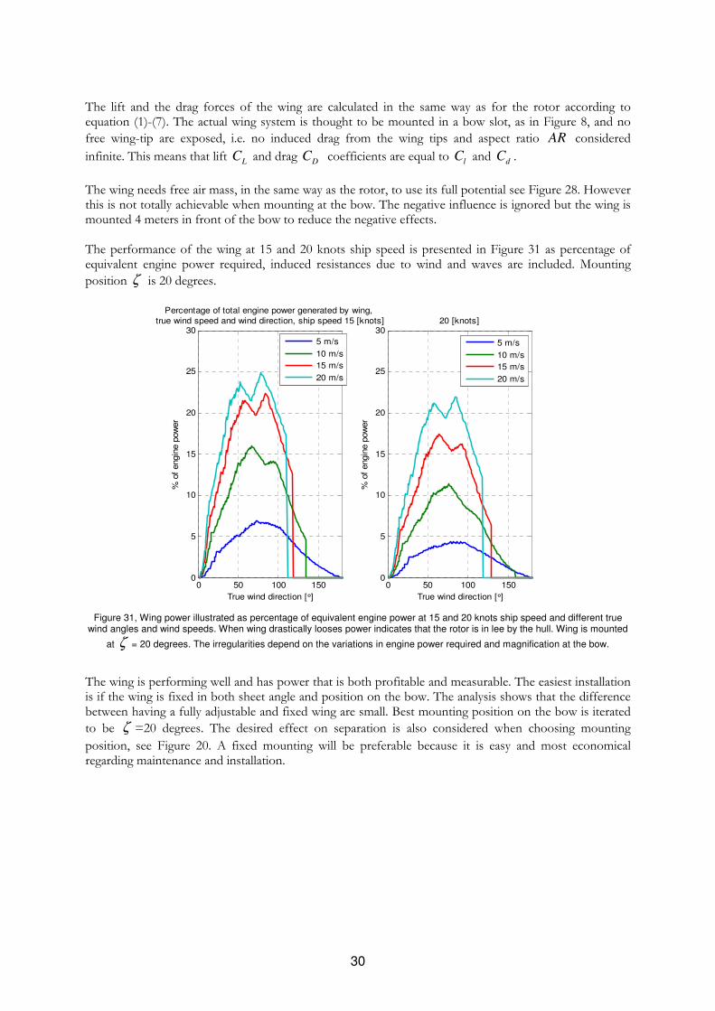
The wing needs free air mass, in the same way as the rotor, to use its full potential see Figure 28. However this is not totally achievable when mounting at the bow. The negative influence is ignored but the wing is mounted 4 meters in front of the bow to reduce the negative effects. The performance of the wing at 15 and 20 knots ship speed is presented in Figure 31 as percentage of equivalent engine power required, induced resistances due to wind and waves are included. Mounting

position ζ is 20 degrees.

0 50 100 1500

5

10

15

20

25

30


% o

f engin

e p

ow

er

Percentage of total engine power generated by wing, true wind speed and wind direction, ship speed 15 [knots]

5 m/s

10 m/s

15 m/s

20 m/s

0 50 100 1500

5

10

15

20

25

30


% o

f engin

e p

ow

er

20 [knots]

5 m/s

10 m/s

15 m/s

20 m/s

Figure 31, Wing power illustrated as percentage of equivalent engine power at 15 and 20 knots ship speed and different true

wind angles and wind speeds. When wing drastically looses power indicates that the rotor is in lee by the hull. Wing is mounted

at ζ = 20 degrees. The irregularities depend on the variations in engine power required and magnification at the bow.

The wing is performing well and has power that is both profitable and measurable. The easiest installation is if the wing is fixed in both sheet angle and position on the bow. The analysis shows that the difference between having a fully adjustable and fixed wing are small. Best mounting position on the bow is iterated

to be ζ =20 degrees. The desired effect on separation is also considered when choosing mounting

position, see Figure 20. A fixed mounting will be preferable because it is easy and most economical regarding maintenance and installation.

31

3.4.3. The Kite

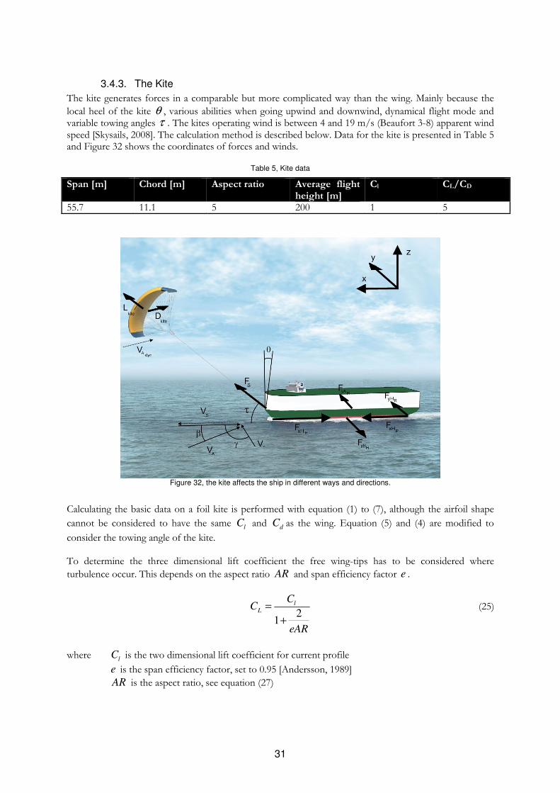
The kite generates forces in a comparable but more complicated way than the wing. Mainly because the

local heel of the kite θ , various abilities when going upwind and downwind, dynamical flight mode and variable towing angles τ . The kites operating wind is between 4 and 19 m/s (Beaufort 3-8) apparent wind speed [Skysails, 2008]. The calculation method is described below. Data for the kite is presented in Table 5 and Figure 32 shows the coordinates of forces and winds.

Table 5, Kite data

Span [m] Chord [m] Aspect ratio Average flight height [m]

Cl CL/CD

55.7 11.1 5 200 1 5

Figure 32, the kite affects the ship in different ways and directions.

Calculating the basic data on a foil kite is performed with equation (1) to (7), although the airfoil shape

cannot be considered to have the same lC and dC as the wing. Equation (5) and (4) are modified to

consider the towing angle of the kite. To determine the three dimensional lift coefficient the free wing-tips has to be considered where

turbulence occur. This depends on the aspect ratio AR and span efficiency factor e .

2

1

lL

CC

eAR

=

+

(25)

where l

C is the two dimensional lift coefficient for current profile

e is the span efficiency factor, set to 0.95 [Andersson, 1989]

AR is the aspect ratio, see equation (27)

32

0

2

LD d D

CC C C

eARπ= + + (26)

where d

C is the two dimensional drag coefficient for current profile

0D

C is the drag from other extremities in this case the lines

An approximate ratio of /L D

C C is set to 5 [Gernez, 2009]. This is used to determine 0D

C , where l

C is

set to 1 and d

C +0D

C is decided so that /L D

C C =5 is fulfilled.

2

bAR

A= (27)

where b is the surface span

A is the area One advantage of the kite is its flight height which is significantly higher than the other systems, here is an average altitude of 200 meters is set. Together with the dynamic flight which increases the apparent wind speed for the system it is a system that can profit from strong and stable winds at high altitude. The area can also be considered to be larger than for any other system used. The big disadvantage is that the kite will not always fly and create lift in the ship’s moving direction. This depends both on the towing angle τ and the kite’s true flying direction. The towing angle is assumed to always be 35 degrees to the water level as it is unsafe if the kite is allowed closer to the water.

The apparent wind speed A

V is used to calculate the forces acting on the ship but the wind speed also

needs to be corrected ~

AV according to [Kuttenkeuler, 2007] for heeling angles θ which are assumed to be shifting between -10 to 10 degrees when the kite flies in dynamic mode.

~

sin cos cos sin2

A AV V aπ

β θ

= − ⋅ (28)

The dynamic wind speed dynA

V of the kite is approximated to two times the actual true wind speed

[Gernez, 2009].

2dynA T

V V= ⋅ (29)

The kite apparent wind speed kiteA

V is the root mean square value of ~

AV and dynA

V according to

( )2

~ 2

kite dynAA A

V V V

= +

(30)

The towing angle τ determines the lifting force direction of the kite kite

L according to

coskite

L L τ= (31)

33

Where L is calculated according to equation (4) using kiteA

V from equation (30). The drag kite

D will stay

unaffected by the towing angle τ but will be affected by the heeling angle θ according to

coskite

D D θ= (32)

Where D is calculated according to equation (5) using ~

AV . The dynamic speed of the kite creates a drag

but of the same size in opposite direction while it flies dynamically. This wind speed is therefore not contributing to the drag resistance of the kite. At downwind the kite will behave more like a spinnaker and use the drag caused by the apparent wind

speed ~

AV to propel the ship. The dynamic wind speed will still create lift in the same way as before. The

total propelling force will consist of the drag from the apparent wind and the lift from the dynamic speed.

The drag coefficient in this case is plated

C =1.18 when the kite is assumed to have the same drag as a plate

[Massey, 1997]. The percentage of total engine power required delivered by the kite at 15 and 20 knots ship speed is presented in Figure 33.

0 50 100 1500

10

20

30

40

50

60

70

80

90

100


% o

f engin

e p

ow

er

Percentage of total engine power generated by kite, true wind speed and wind direction, ship speed 15 [knots]

5 m/s

10 m/s

15 m/s

0 50 100 1500

10

20

30

40

50

60

70

80

90

100


% o

f engin

e p

ow

er

20 [knots]

5 m/s

10 m/s

15 m/s

Figure 33, Kite power illustrated as percentage of equivalent engine power at 15 and 20 knots ship speed and different true wind angles and wind speeds, note that 20 m/s is not presented as it is assumed to be too windy. The sudden loss of power represents the recovery of the kite due to weak or strong winds. The dip at 15 m/s ~160 degrees shows the change of mode

from upwind to downwind.

The kite is performing well but is a more complex system than the rotor or wing. The kite is a realizable system, provided by Skysails and can be mounted onboard the ship Fedora. The irregularities in Figure 33 depend on the variations in engine power required, wind speed boundary values and mode shifting between upwind and downwind. However the performance per area, comparing to the smaller and simpler systems that the rotor and wing system represent is not as good.

34

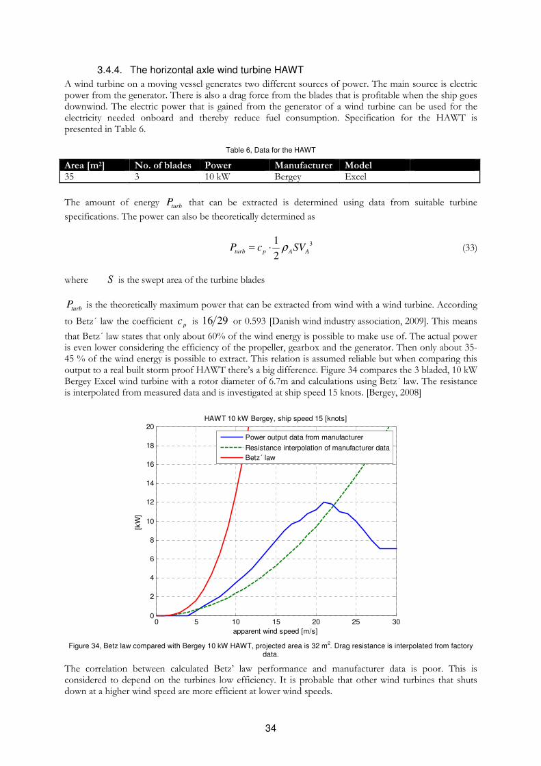
3.4.4. The horizontal axle wind turbine HAWT

A wind turbine on a moving vessel generates two different sources of power. The main source is electric power from the generator. There is also a drag force from the blades that is profitable when the ship goes downwind. The electric power that is gained from the generator of a wind turbine can be used for the electricity needed onboard and thereby reduce fuel consumption. Specification for the HAWT is presented in Table 6.

Table 6, Data for the HAWT

Area [m2] No. of blades Power Manufacturer Model 35 3 10 kW Bergey Excel

The amount of energy turb

P that can be extracted is determined using data from suitable turbine

specifications. The power can also be theoretically determined as

31

2turb p A A

P c SVρ= ⋅ (33)

where S is the swept area of the turbine blades

turbP is the theoretically maximum power that can be extracted from wind with a wind turbine. According

to Betz´ law the coefficient p

c is 16 29 or 0.593 [Danish wind industry association, 2009]. This means

that Betz´ law states that only about 60% of the wind energy is possible to make use of. The actual power is even lower considering the efficiency of the propeller, gearbox and the generator. Then only about 35-45 % of the wind energy is possible to extract. This relation is assumed reliable but when comparing this output to a real built storm proof HAWT there’s a big difference. Figure 34 compares the 3 bladed, 10 kW Bergey Excel wind turbine with a rotor diameter of 6.7m and calculations using Betz´ law. The resistance is interpolated from measured data and is investigated at ship speed 15 knots. [Bergey, 2008]

0 5 10 15 20 25 300

2

4

6

8

10

12

14

16

18

20

apparent wind speed [m/s]

[kW

]

HAWT 10 kW Bergey, ship speed 15 [knots]

Power output data from manufacturer

Resistance interpolation of manufacturer data

Betz´ law

Figure 34, Betz law compared with Bergey 10 kW HAWT, projected area is 32 m

2. Drag resistance is interpolated from factory

data.

The correlation between calculated Betz’ law performance and manufacturer data is poor. This is considered to depend on the turbines low efficiency. It is probable that other wind turbines that shuts down at a higher wind speed are more efficient at lower wind speeds.

35

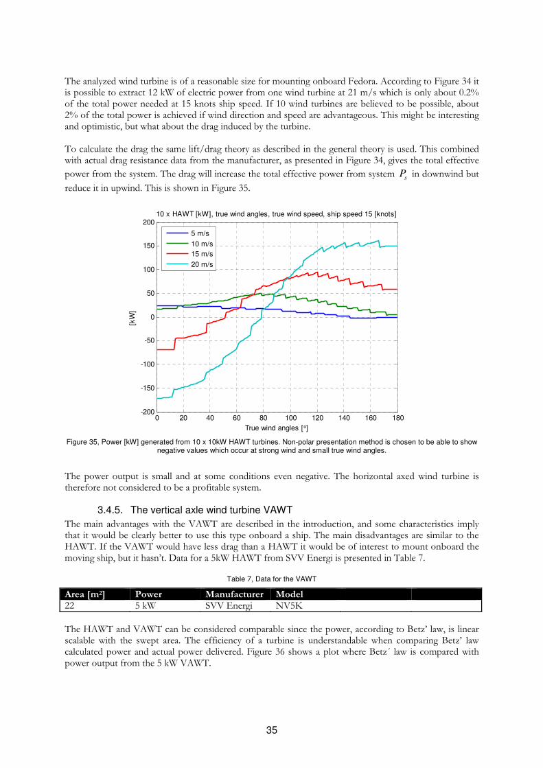
The analyzed wind turbine is of a reasonable size for mounting onboard Fedora. According to Figure 34 it is possible to extract 12 kW of electric power from one wind turbine at 21 m/s which is only about 0.2% of the total power needed at 15 knots ship speed. If 10 wind turbines are believed to be possible, about 2% of the total power is achieved if wind direction and speed are advantageous. This might be interesting and optimistic, but what about the drag induced by the turbine. To calculate the drag the same lift/drag theory as described in the general theory is used. This combined with actual drag resistance data from the manufacturer, as presented in Figure 34, gives the total effective

power from the system. The drag will increase the total effective power from system s

P in downwind but

reduce it in upwind. This is shown in Figure 35.

0 20 40 60 80 100 120 140 160 180-200

-150

-100

-50

0

50

100

150

200

True wind angles [°]

[kW

]

10 x HAWT [kW], true wind angles, true wind speed, ship speed 15 [knots]

5 m/s

10 m/s

15 m/s

20 m/s

Figure 35, Power [kW] generated from 10 x 10kW HAWT turbines. Non-polar presentation method is chosen to be able to show

negative values which occur at strong wind and small true wind angles.

The power output is small and at some conditions even negative. The horizontal axed wind turbine is therefore not considered to be a profitable system.

3.4.5. The vertical axle wind turbine VAWT

The main advantages with the VAWT are described in the introduction, and some characteristics imply that it would be clearly better to use this type onboard a ship. The main disadvantages are similar to the HAWT. If the VAWT would have less drag than a HAWT it would be of interest to mount onboard the moving ship, but it hasn’t. Data for a 5kW HAWT from SVV Energi is presented in Table 7.

Table 7, Data for the VAWT

Area [m2] Power Manufacturer Model 22 5 kW SVV Energi NV5K

The HAWT and VAWT can be considered comparable since the power, according to Betz’ law, is linear scalable with the swept area. The efficiency of a turbine is understandable when comparing Betz’ law calculated power and actual power delivered. Figure 36 shows a plot where Betz´ law is compared with power output from the 5 kW VAWT.

36

0 5 10 15 20 25 300

2

4

6

8

10

12

14

16

18

20

wind speed [m/s]

[kW

]

VAWT 5kW SVV Energi AB, ship speed 15 [knots]

Power output data from manufacturer

Resistance interpolation of manufacturer data

Betz´ law

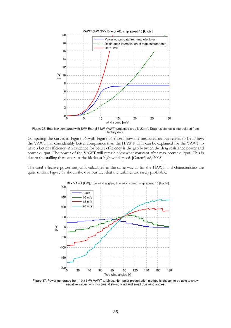
Figure 36, Betz law compared with SVV Energi 5 kW VAWT, projected area is 22 m

2. Drag resistance is interpolated from

factory data.

Comparing the curves in Figure 36 with Figure 34 shows how the measured output relates to Betz´ law; the VAWT has considerably better compliance than the HAWT. This can be explained for the VAWT to have a better efficiency. An evidence for better efficiency is the gap between the drag resistance power and power output. The power of the VAWT will remain somewhat constant after max power output. This is due to the stalling that occurs at the blades at high wind speed. [Gatenfjord, 2008] The total effective power output is calculated in the same way as for the HAWT and characteristics are quite similar. Figure 37 shows the obvious fact that the turbines are rarely profitable.

0 20 40 60 80 100 120 140 160 180-200

-150

-100

-50

0

50

100

150

200

True wind angles [°]

[kW

]

10 x VAWT [kW], true wind angles, true wind speed, ship speed 15 [knots]

5 m/s

10 m/s

15 m/s

20 m/s

Figure 37, Power generated from 10 x 5kW VAWT turbines. Non-polar presentation method is chosen to be able to show

negative values which occurs at strong wind and small true wind angles.

37

The vertical axed wind turbine doesn’t seem to be a profitable solution. An alternative solution would be to have wind turbines that are foldable and only use them at downwind or at port. This could be interesting considering the environmental profile, but probably not economic since they can rarely be used and are expensive investments.

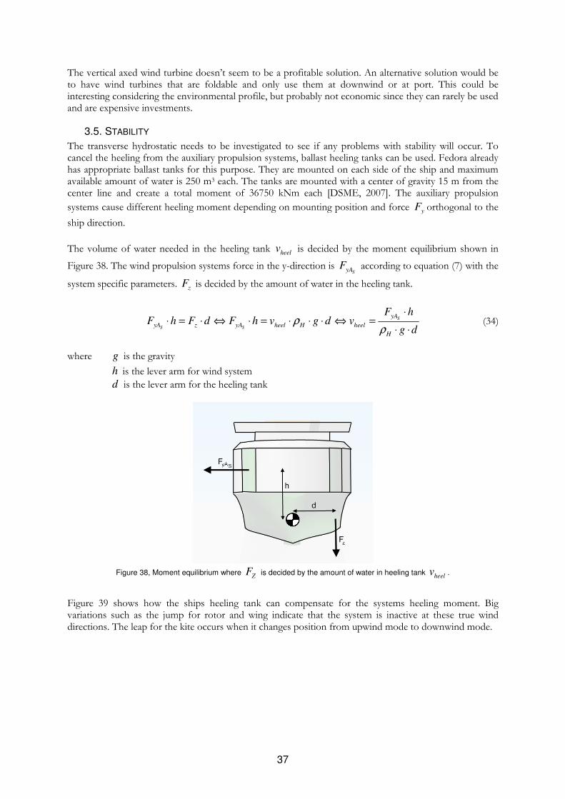
3.5. STABILITY

The transverse hydrostatic needs to be investigated to see if any problems with stability will occur. To cancel the heeling from the auxiliary propulsion systems, ballast heeling tanks can be used. Fedora already has appropriate ballast tanks for this purpose. They are mounted on each side of the ship and maximum available amount of water is 250 m3 each. The tanks are mounted with a center of gravity 15 m from the center line and create a total moment of 36750 kNm each [DSME, 2007]. The auxiliary propulsion

systems cause different heeling moment depending on mounting position and force y

F orthogonal to the

ship direction.

The volume of water needed in the heeling tank heel

v is decided by the moment equilibrium shown in

Figure 38. The wind propulsion systems force in the y-direction is SyA

F according to equation (7) with the

system specific parameters. z

F is decided by the amount of water in the heeling tank.

S

S S

yA

yA z yA heel H heel

H

F hF h F d F h v g d v

g dρ

ρ

⋅⋅ = ⋅ ⇔ ⋅ = ⋅ ⋅ ⋅ ⇔ =

⋅ ⋅ (34)

where g is the gravity

h is the lever arm for wind system

d is the lever arm for the heeling tank

Figure 38, Moment equilibrium where

ZF is decided by the amount of water in heeling tank

heelv .

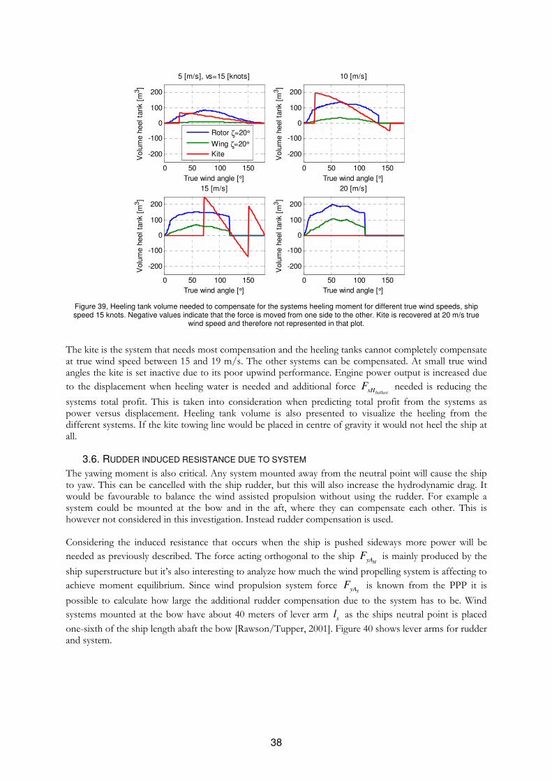
Figure 39 shows how the ships heeling tank can compensate for the systems heeling moment. Big variations such as the jump for rotor and wing indicate that the system is inactive at these true wind directions. The leap for the kite occurs when it changes position from upwind mode to downwind mode.

38

0 50 100 150

-200

-100

0

100

200


Volu

me h

eel ta

nk [

m3]

5 [m/s], vs=15 [knots]

0 50 100 150

-200

-100

0

100

200

10 [m/s]


Volu

me h

eel ta

nk [

m3]

0 50 100 150

-200

-100

0

100

200

15 [m/s]


Volu

me h

eel ta

nk [

m3]

0 50 100 150

-200

-100

0

100

200

20 [m/s]


Volu

me h

eel ta

nk [

m3]

Rotor ζ=20°

Wing ζ=20°Kite

Figure 39, Heeling tank volume needed to compensate for the systems heeling moment for different true wind speeds, ship speed 15 knots. Negative values indicate that the force is moved from one side to the other. Kite is recovered at 20 m/s true

wind speed and therefore not represented in that plot.

The kite is the system that needs most compensation and the heeling tanks cannot completely compensate at true wind speed between 15 and 19 m/s. The other systems can be compensated. At small true wind angles the kite is set inactive due to its poor upwind performance. Engine power output is increased due

to the displacement when heeling water is needed and additional force ballastxH

F needed is reducing the

systems total profit. This is taken into consideration when predicting total profit from the systems as power versus displacement. Heeling tank volume is also presented to visualize the heeling from the different systems. If the kite towing line would be placed in centre of gravity it would not heel the ship at all.

3.6. RUDDER INDUCED RESISTANCE DUE TO SYSTEM

The yawing moment is also critical. Any system mounted away from the neutral point will cause the ship to yaw. This can be cancelled with the ship rudder, but this will also increase the hydrodynamic drag. It would be favourable to balance the wind assisted propulsion without using the rudder. For example a system could be mounted at the bow and in the aft, where they can compensate each other. This is however not considered in this investigation. Instead rudder compensation is used. Considering the induced resistance that occurs when the ship is pushed sideways more power will be

needed as previously described. The force acting orthogonal to the ship HyA

F is mainly produced by the

ship superstructure but it’s also interesting to analyze how much the wind propelling system is affecting to

achieve moment equilibrium. Since wind propulsion system force SyA

F is known from the PPP it is

possible to calculate how large the additional rudder compensation due to the system has to be. Wind

systems mounted at the bow have about 40 meters of lever arm s

l as the ships neutral point is placed

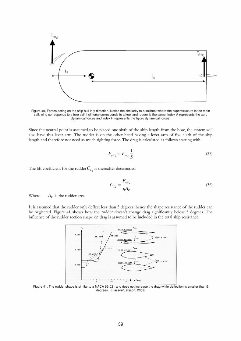
one-sixth of the ship length abaft the bow [Rawson/Tupper, 2001]. Figure 40 shows lever arms for rudder and system.

39

Figure 40, Forces acting on the ship hull in y-direction. Notice the similarity to a sailboat where the superstructure is the main

sail, wing corresponds to a fore sail, hull force corresponds to a keel and rudder is the same. Index A represents the aero dynamical forces and index H represents the hydro dynamical forces.

Since the neutral point is assumed to be placed one sixth of the ship length from the bow, the system will also have this lever arm. The rudder is on the other hand having a lever arm of five sixth of the ship length and therefore not need as much righting force. The drag is calculated as follows starting with

1

5R SyH yAF F= (35)

The lift coefficient for the rudderRL

C is thereafter determined.

R

R

yH

L

R

FC

qA= (36)

Where R

A is the rudder area

It is assumed that the rudder only deflect less than 5 degrees, hence the shape resistance of the rudder can be neglected. Figure 41 shows how the rudder doesn’t change drag significantly below 5 degrees. The influence of the rudder section shape on drag is assumed to be included in the total ship resistance.

Figure 41, The rudder shape is similar to a NACA 63-021 and does not increase the drag while deflection is smaller than 5

degrees. [Eliasson/Larsson, 2002]

40

With these assumptions there is only the rudders induced drag RD

C left according to

2

R

R

L

D

R

CC

eARπ= (37)

Where R

AR is the rudder aspect ratio

Knowing the rudders induced drag it is possible to know how the ships total resistance is affected by

calculating the hydrodynamic force caused by the rudder in x-direction RxH

F .

R RxH R R D

F D qA C= = (38)

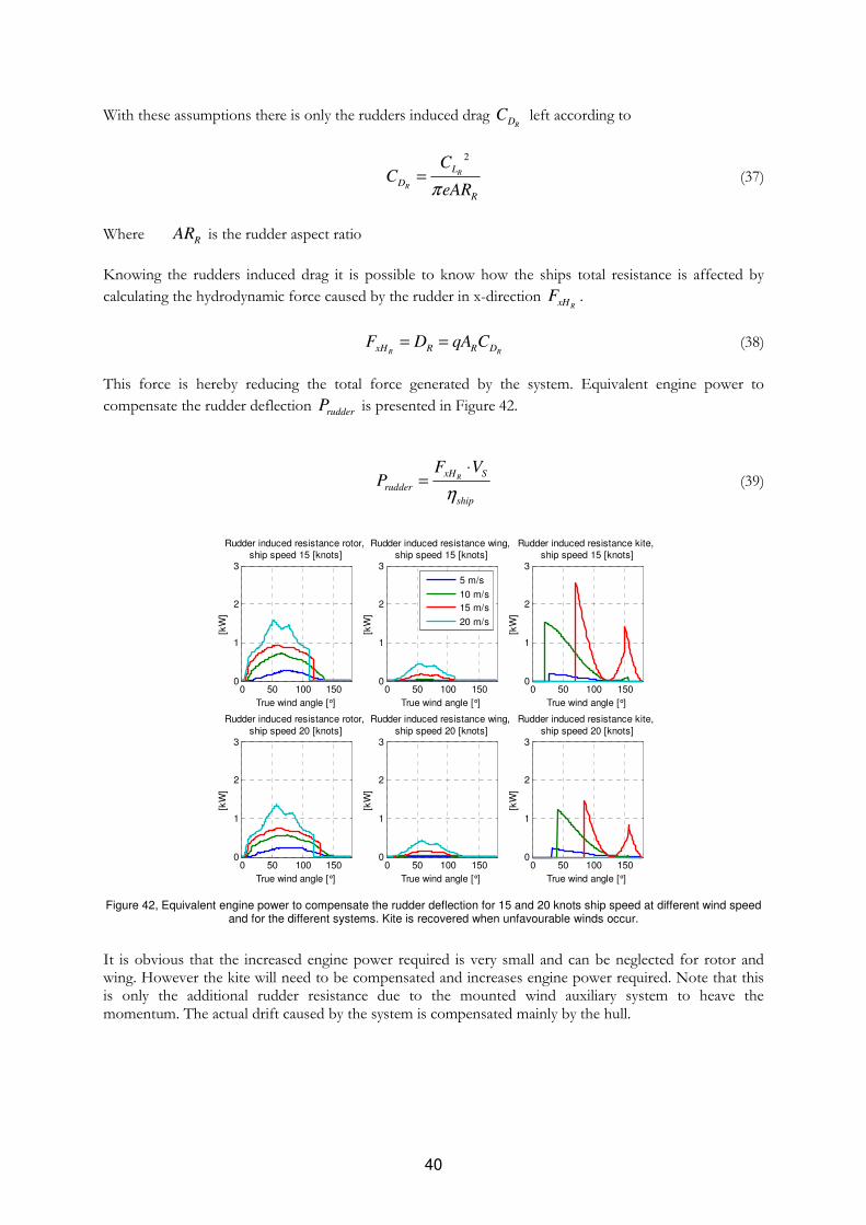
This force is hereby reducing the total force generated by the system. Equivalent engine power to

compensate the rudder deflection rudder

P is presented in Figure 42.

RxH S

rudder

ship

F VP

η

⋅= (39)

0 50 100 1500

1

2

3

Rudder induced resistance rotor, ship speed 15 [knots]

[kW

]


0 50 100 1500

1

2

3

Rudder induced resistance wing, ship speed 15 [knots]

[kW

]


0 50 100 1500

1

2

3

Rudder induced resistance kite, ship speed 15 [knots]

[kW

]


5 m/s

10 m/s

15 m/s

20 m/s

0 50 100 1500

1

2

3

Rudder induced resistance rotor, ship speed 20 [knots]

[kW

]


0 50 100 1500

1

2

3

Rudder induced resistance wing, ship speed 20 [knots]

[kW

]


0 50 100 1500

1

2

3

Rudder induced resistance kite, ship speed 20 [knots]

[kW

]


Figure 42, Equivalent engine power to compensate the rudder deflection for 15 and 20 knots ship speed at different wind speed

and for the different systems. Kite is recovered when unfavourable winds occur.

It is obvious that the increased engine power required is very small and can be neglected for rotor and wing. However the kite will need to be compensated and increases engine power required. Note that this is only the additional rudder resistance due to the mounted wind auxiliary system to heave the momentum. The actual drift caused by the system is compensated mainly by the hull.

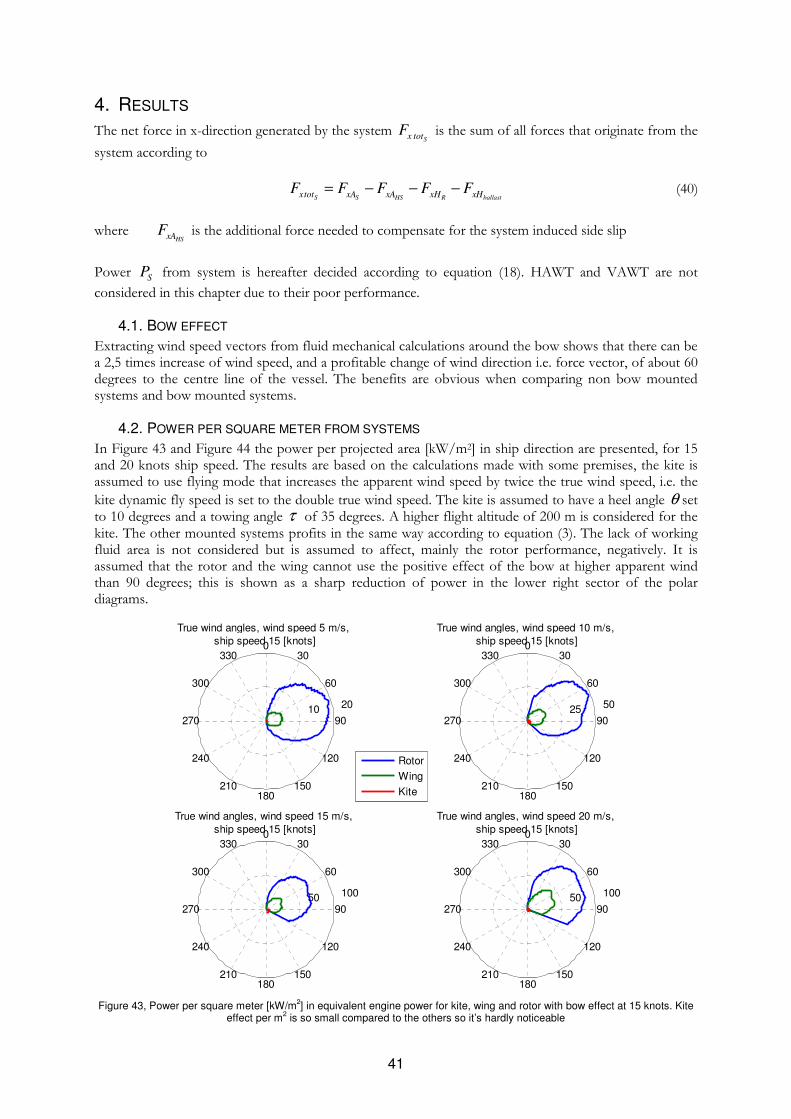
41

4. RESULTS

The net force in x-direction generated by the system Sx tot

F is the sum of all forces that originate from the

system according to

S S HS R ballastxtot xA xA xH xH

F F F F F= − − − (40)

where HSxA

F is the additional force needed to compensate for the system induced side slip

Power S

P from system is hereafter decided according to equation (18). HAWT and VAWT are not

considered in this chapter due to their poor performance.

4.1. BOW EFFECT

Extracting wind speed vectors from fluid mechanical calculations around the bow shows that there can be a 2,5 times increase of wind speed, and a profitable change of wind direction i.e. force vector, of about 60 degrees to the centre line of the vessel. The benefits are obvious when comparing non bow mounted systems and bow mounted systems.

4.2. POWER PER SQUARE METER FROM SYSTEMS

In Figure 43 and Figure 44 the power per projected area [kW/m2] in ship direction are presented, for 15 and 20 knots ship speed. The results are based on the calculations made with some premises, the kite is assumed to use flying mode that increases the apparent wind speed by twice the true wind speed, i.e. the

kite dynamic fly speed is set to the double true wind speed. The kite is assumed to have a heel angle θ set to 10 degrees and a towing angle τ of 35 degrees. A higher flight altitude of 200 m is considered for the kite. The other mounted systems profits in the same way according to equation (3). The lack of working fluid area is not considered but is assumed to affect, mainly the rotor performance, negatively. It is assumed that the rotor and the wing cannot use the positive effect of the bow at higher apparent wind than 90 degrees; this is shown as a sharp reduction of power in the lower right sector of the polar diagrams.

10 20

30

210

60

240

90270

120

300

150

330

180

0

True wind angles, wind speed 5 m/s, ship speed 15 [knots]

Rotor

Wing

Kite

25 50

30

210

60

240

90270

120

300

150

330

180

0


50 100

30

210

60

240

90270

120

300

150

330

180

0


50 100

30

210

60

240

90270

120

300

150

330

180

0


Figure 43, Power per square meter [kW/m2] in equivalent engine power for kite, wing and rotor with bow effect at 15 knots. Kite

effect per m2 is so small compared to the others so it’s hardly noticeable

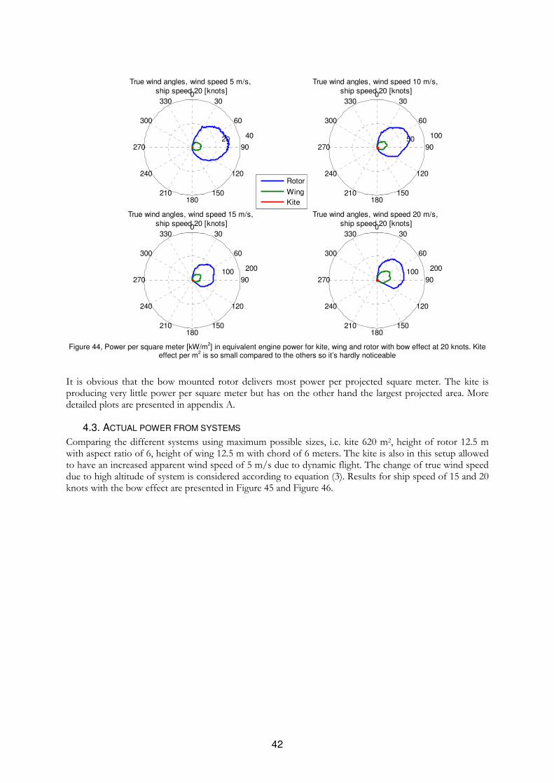
42

50 100

30

210

60

240

90270

120

300

150

330

180

0


100 200

30

210

60

240

90270

120

300

150

330

180

0


100 200

30

210

60

240

90270

120

300

150

330

180

0


20 40

30

210

60

240

90270

120

300

150

330

180

0


Rotor

Wing

Kite

Figure 44, Power per square meter [kW/m2] in equivalent engine power for kite, wing and rotor with bow effect at 20 knots. Kite

effect per m2 is so small compared to the others so it’s hardly noticeable

It is obvious that the bow mounted rotor delivers most power per projected square meter. The kite is producing very little power per square meter but has on the other hand the largest projected area. More detailed plots are presented in appendix A.

4.3. ACTUAL POWER FROM SYSTEMS

Comparing the different systems using maximum possible sizes, i.e. kite 620 m2, height of rotor 12.5 m with aspect ratio of 6, height of wing 12.5 m with chord of 6 meters. The kite is also in this setup allowed to have an increased apparent wind speed of 5 m/s due to dynamic flight. The change of true wind speed due to high altitude of system is considered according to equation (3). Results for ship speed of 15 and 20 knots with the bow effect are presented in Figure 45 and Figure 46.

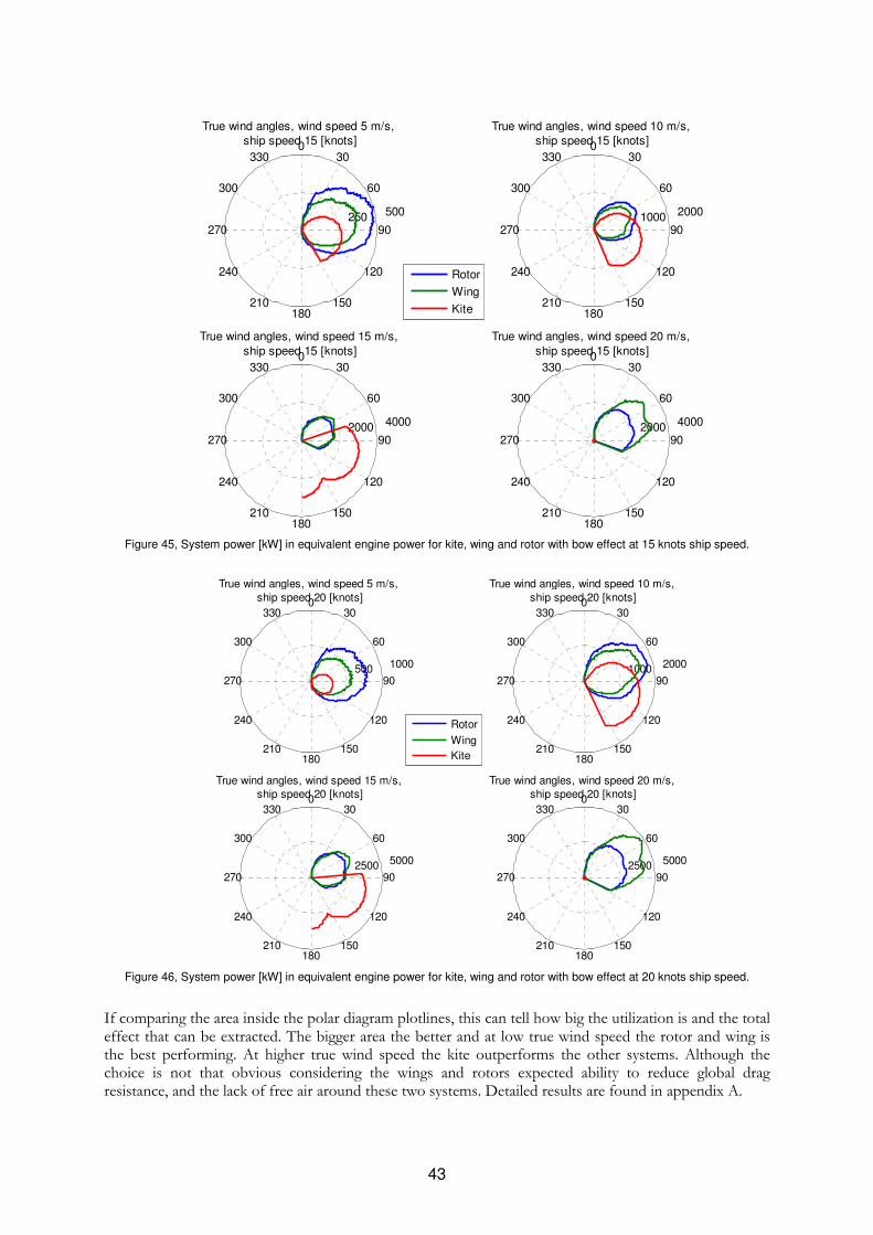
43

2000 4000

30

210

60

240

90270

120

300

150

330

180

0

True wind angles, wind speed 20 m/s,


250 500

30

210

60

240

90270

120

300

150

330

180

0


1000 2000

30

210

60

240

90270

120

300

150

330

180

0


2000 4000

30

210

60

240

90270

120

300

150

330

180

0



Rotor

Wing

Kite

Figure 45, System power [kW] in equivalent engine power for kite, wing and rotor with bow effect at 15 knots ship speed.

2500 5000

30

210

60

240

90270

120

300

150

330

180

0


500 1000

30

210

60

240

90270

120

300

150

330

180

0



1000 2000

30

210

60

240

90270

120

300

150

330

180

0



Rotor

Wing

Kite

2500 5000

30

210

60

240

90270

120

300

150

330

180

0


Figure 46, System power [kW] in equivalent engine power for kite, wing and rotor with bow effect at 20 knots ship speed.

If comparing the area inside the polar diagram plotlines, this can tell how big the utilization is and the total effect that can be extracted. The bigger area the better and at low true wind speed the rotor and wing is the best performing. At higher true wind speed the kite outperforms the other systems. Although the choice is not that obvious considering the wings and rotors expected ability to reduce global drag resistance, and the lack of free air around these two systems. Detailed results are found in appendix A.

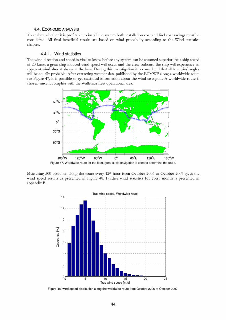
44

4.4. ECONOMIC ANALYSIS

To analyze whether it is profitable to install the system both installation cost and fuel cost savings must be considered. All final beneficial results are based on wind probability according to the Wind statistics chapter.

4.4.1. Wind statistics

The wind direction and speed is vital to know before any system can be assumed superior. At a ship speed of 20 knots a great ship induced wind speed will occur and the crew onboard the ship will experience an apparent wind almost always at the bow. During this investigation it is considered that all true wind angles will be equally probable. After extracting weather data published by the ECMWF along a worldwide route see Figure 47, it is possible to get statistical information about the wind strengths. A worldwide route is chosen since it complies with the Wallenius fleet operational area.

180oW 120oW 60oW 0o 60oE 120oE 180oW

60oS

30oS

0o

30oN

60oN

Figure 47, Worldwide route for the fleet, great circle navigation is used to determine the route.

Measuring 500 positions along the route every 12th hour from October 2006 to October 2007 gives the wind speed results as presented in Figure 48. Further wind statistics for every month is presented in appendix B.

0 5 10 15 20 250

2

4

6

8

10

12

14

Occura

nce [

%]

True wind speed [m/s]

True wind speed, Worldwide route

Figure 48, wind speed distribution along the worldwide route from October 2006 to October 2007.

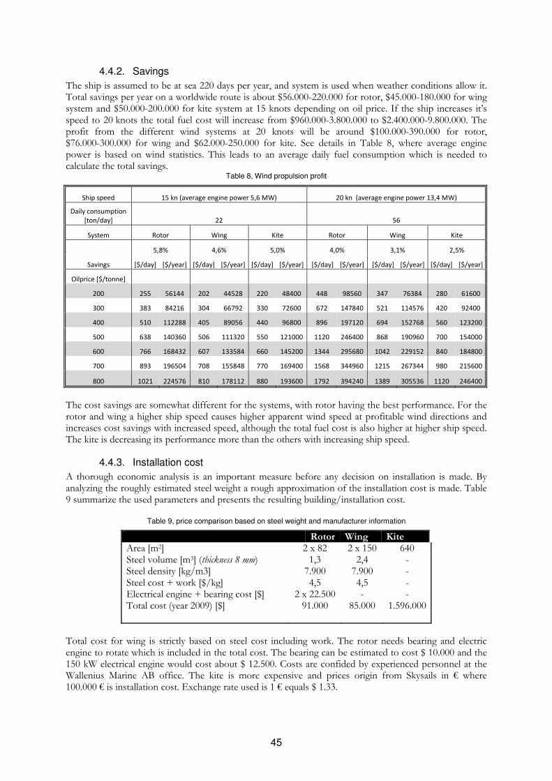
45

4.4.2. Savings

The ship is assumed to be at sea 220 days per year, and system is used when weather conditions allow it. Total savings per year on a worldwide route is about $56.000-220.000 for rotor, $45.000-180.000 for wing system and $50.000-200.000 for kite system at 15 knots depending on oil price. If the ship increases it’s speed to 20 knots the total fuel cost will increase from $960.000-3.800.000 to $2.400.000-9.800.000. The profit from the different wind systems at 20 knots will be around $100.000-390.000 for rotor, $76.000-300.000 for wing and $62.000-250.000 for kite. See details in Table 8, where average engine power is based on wind statistics. This leads to an average daily fuel consumption which is needed to calculate the total savings.

Table 8, Wind propulsion profit

Ship speed 15 kn (average engine power 5,6 MW) 20 kn (average engine power 13,4 MW)

Daily consumption

[ton/day] 22 56

System Rotor Wing Kite Rotor Wing Kite

Savings

5,8% 4,6% 5,0% 4,0% 3,1% 2,5%

[$/day] [$/year] [$/day] [$/year] [$/day] [$/year] [$/day] [$/year] [$/day] [$/year] [$/day] [$/year]

Oilprice [$/tonne]

200 255 56144 202 44528 220 48400 448 98560 347 76384 280 61600

300 383 84216 304 66792 330 72600 672 147840 521 114576 420 92400

400 510 112288 405 89056 440 96800 896 197120 694 152768 560 123200

500 638 140360 506 111320 550 121000 1120 246400 868 190960 700 154000

600 766 168432 607 133584 660 145200 1344 295680 1042 229152 840 184800

700 893 196504 708 155848 770 169400 1568 344960 1215 267344 980 215600

800 1021 224576 810 178112 880 193600 1792 394240 1389 305536 1120 246400

The cost savings are somewhat different for the systems, with rotor having the best performance. For the rotor and wing a higher ship speed causes higher apparent wind speed at profitable wind directions and increases cost savings with increased speed, although the total fuel cost is also higher at higher ship speed. The kite is decreasing its performance more than the others with increasing ship speed.

4.4.3. Installation cost

A thorough economic analysis is an important measure before any decision on installation is made. By analyzing the roughly estimated steel weight a rough approximation of the installation cost is made. Table 9 summarize the used parameters and presents the resulting building/installation cost.

Table 9, price comparison based on steel weight and manufacturer information

Rotor Wing Kite Area [m2] 2 x 82 2 x 150 640 Steel volume [m3] (thickness 8 mm) 1,3 2,4 - Steel density [kg/m3] 7.900 7.900 - Steel cost + work [$/kg] 4,5 4,5 - Electrical engine + bearing cost [$] 2 x 22.500 - - Total cost (year 2009) [$] 91.000 85.000 1.596.000

Total cost for wing is strictly based on steel cost including work. The rotor needs bearing and electric engine to rotate which is included in the total cost. The bearing can be estimated to cost $ 10.000 and the 150 kW electrical engine would cost about $ 12.500. Costs are confided by experienced personnel at the Wallenius Marine AB office. The kite is more expensive and prices origin from Skysails in € where 100.000 € is installation cost. Exchange rate used is 1 € equals $ 1.33.

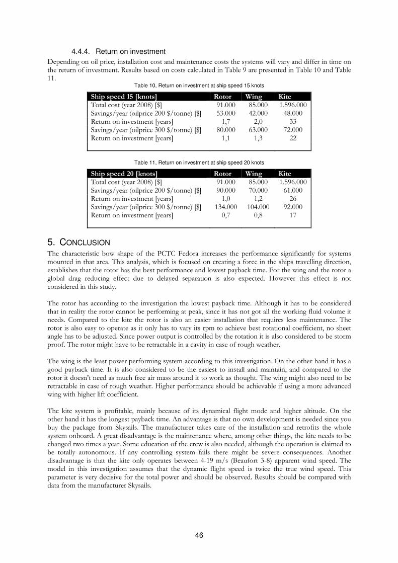
46

4.4.4. Return on investment

Depending on oil price, installation cost and maintenance costs the systems will vary and differ in time on the return of investment. Results based on costs calculated in Table 9 are presented in Table 10 and Table 11.

Table 10, Return on investment at ship speed 15 knots

Ship speed 15 [knots] Rotor Wing Kite Total cost (year 2008) [$] 91.000 85.000 1.596.000 Savings/year (oilprice 200 $/tonne) [$] 53.000 42.000 48.000 Return on investment [years] 1,7 2,0 33 Savings/year (oilprice 300 $/tonne) [$] 80.000 63.000 72.000 Return on investment [years] 1,1 1,3 22

Table 11, Return on investment at ship speed 20 knots

Ship speed 20 [knots] Rotor Wing Kite Total cost (year 2008) [$] 91.000 85.000 1.596.000 Savings/year (oilprice 200 $/tonne) [$] 90.000 70.000 61.000 Return on investment [years] 1,0 1,2 26 Savings/year (oilprice 300 $/tonne) [$] 134.000 104.000 92.000 Return on investment [years] 0,7 0,8 17

5. CONCLUSION The characteristic bow shape of the PCTC Fedora increases the performance significantly for systems mounted in that area. This analysis, which is focused on creating a force in the ships travelling direction, establishes that the rotor has the best performance and lowest payback time. For the wing and the rotor a global drag reducing effect due to delayed separation is also expected. However this effect is not considered in this study. The rotor has according to the investigation the lowest payback time. Although it has to be considered that in reality the rotor cannot be performing at peak, since it has not got all the working fluid volume it needs. Compared to the kite the rotor is also an easier installation that requires less maintenance. The rotor is also easy to operate as it only has to vary its rpm to achieve best rotational coefficient, no sheet angle has to be adjusted. Since power output is controlled by the rotation it is also considered to be storm proof. The rotor might have to be retractable in a cavity in case of rough weather. The wing is the least power performing system according to this investigation. On the other hand it has a good payback time. It is also considered to be the easiest to install and maintain, and compared to the rotor it doesn’t need as much free air mass around it to work as thought. The wing might also need to be retractable in case of rough weather. Higher performance should be achievable if using a more advanced wing with higher lift coefficient. The kite system is profitable, mainly because of its dynamical flight mode and higher altitude. On the other hand it has the longest payback time. An advantage is that no own development is needed since you buy the package from Skysails. The manufacturer takes care of the installation and retrofits the whole system onboard. A great disadvantage is the maintenance where, among other things, the kite needs to be changed two times a year. Some education of the crew is also needed, although the operation is claimed to be totally autonomous. If any controlling system fails there might be severe consequences. Another disadvantage is that the kite only operates between 4-19 m/s (Beaufort 3-8) apparent wind speed. The model in this investigation assumes that the dynamic flight speed is twice the true wind speed. This parameter is very decisive for the total power and should be observed. Results should be compared with data from the manufacturer Skysails.

47

Overall results conclude that the wing system is preferable. It has good payback investment, assumes to have global drag reducing effects, is cheap to build and maintain and has a measurable performance. The wind turbines are not considered profitable.

6. RECOMMENDATIONS The advantage is clear concerning the theoretical fuel savings determined, and this should be verified. My recommendations would be to verify the results of the wing and rotor in a wind tunnel test. The global effect of the wing and rotor seems interesting since it could reduce the fuel consumption even more. This might also be settled during a full three dimensional CFD-analysis. Kite performance should be verified by Skysails, as they will deliver an own analysis of fuel savings established. Installation of the wing and the rotor should be investigated more thoroughly regarding solid mechanics and manufacturing.

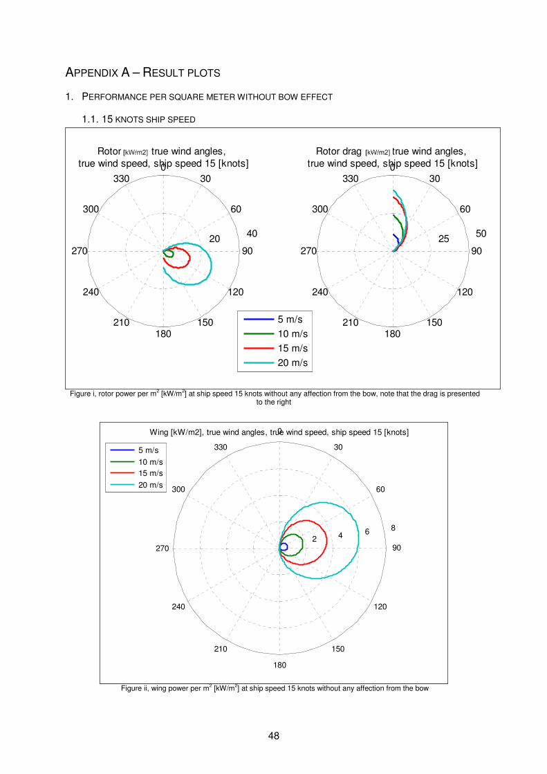
48

APPENDIX A – RESULT PLOTS

1. PERFORMANCE PER SQUARE METER WITHOUT BOW EFFECT

1.1. 15 KNOTS SHIP SPEED

20 40

30

210

60

240

90270

120

300

150

330

180

0

Rotor [kW], true wind angles, true wind speed, ship speed 15 [knots]

5 m/s

10 m/s

15 m/s

20 m/s

25 50

30

210

60

240

90270

120

300

150

330

180

0

Rotor drag [kW], true wind angles, true wind speed, ship speed 15 [knots]

Figure i, rotor power per m2 [kW/m2] at ship speed 15 knots without any affection from the bow, note that the drag is presented

to the right

2 4 6 8

30

210

60

240

90270

120

300

150

330

180

0Wing [kW/m2], true wind angles, true wind speed, ship speed 15 [knots]

5 m/s

10 m/s

15 m/s

20 m/s

Figure ii, wing power per m2 [kW/m2] at ship speed 15 knots without any affection from the bow

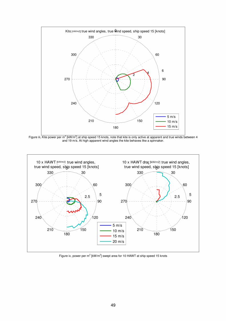
49

2 4

6

30

210

60

240

90270

120

300

150

330

180

0Kite [kW], true wind angles, true wind speed, ship speed 15 [knots]

5 m/s

10 m/s

15 m/s

Figure iii, Kite power per m2 [kW/m2] at ship speed 15 knots, note that kite is only active at apparent and true winds between 4

and 19 m/s. At high apparent wind angles the kite behaves like a spinnaker.

2.5 5

30

210

60

240

90270

120

300

150

330

180

0


5 m/s

10 m/s

15 m/s

20 m/s

2.5 5

30

210

60

240

90270

120

300

150

330

180

0

10 x HAWT drag [kW], true wind angles, true wind speed, ship speed 15 [knots]

Figure iv, power per m2 [kW/m2] swept area for 10 HAWT at ship speed 15 knots

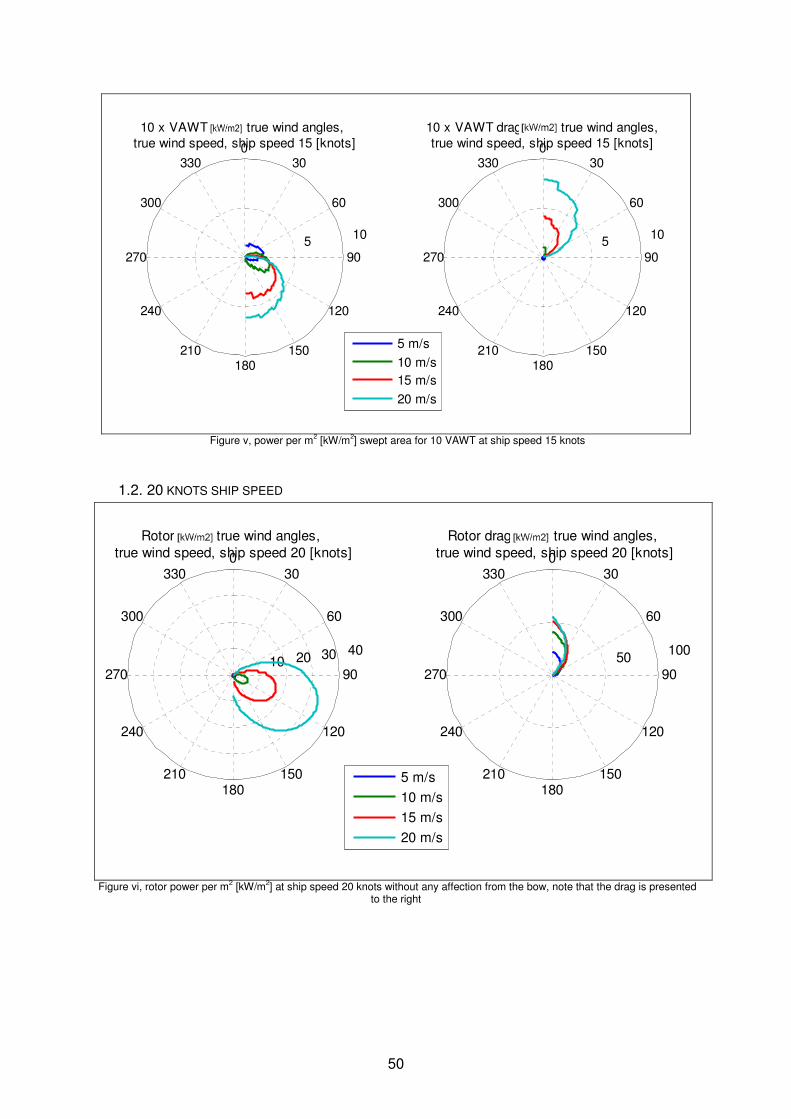
50

5 10

30

210

60

240

90270

120

300

150

330

180

0


5 m/s

10 m/s

15 m/s

20 m/s

5 10

30

210

60

240

90270

120

300

150

330

180

0

10 x VAWT drag [kW], true wind angles,true wind speed, ship speed 15 [knots]

Figure v, power per m2 [kW/m2] swept area for 10 VAWT at ship speed 15 knots


10 20 30 40

30

210

60

240

90270

120

300

150

330

180

0


5 m/s

10 m/s

15 m/s

20 m/s

50 100

30

210

60

240

90270

120

300

150

330

180

0


Figure vi, rotor power per m2 [kW/m2] at ship speed 20 knots without any affection from the bow, note that the drag is presented

to the right

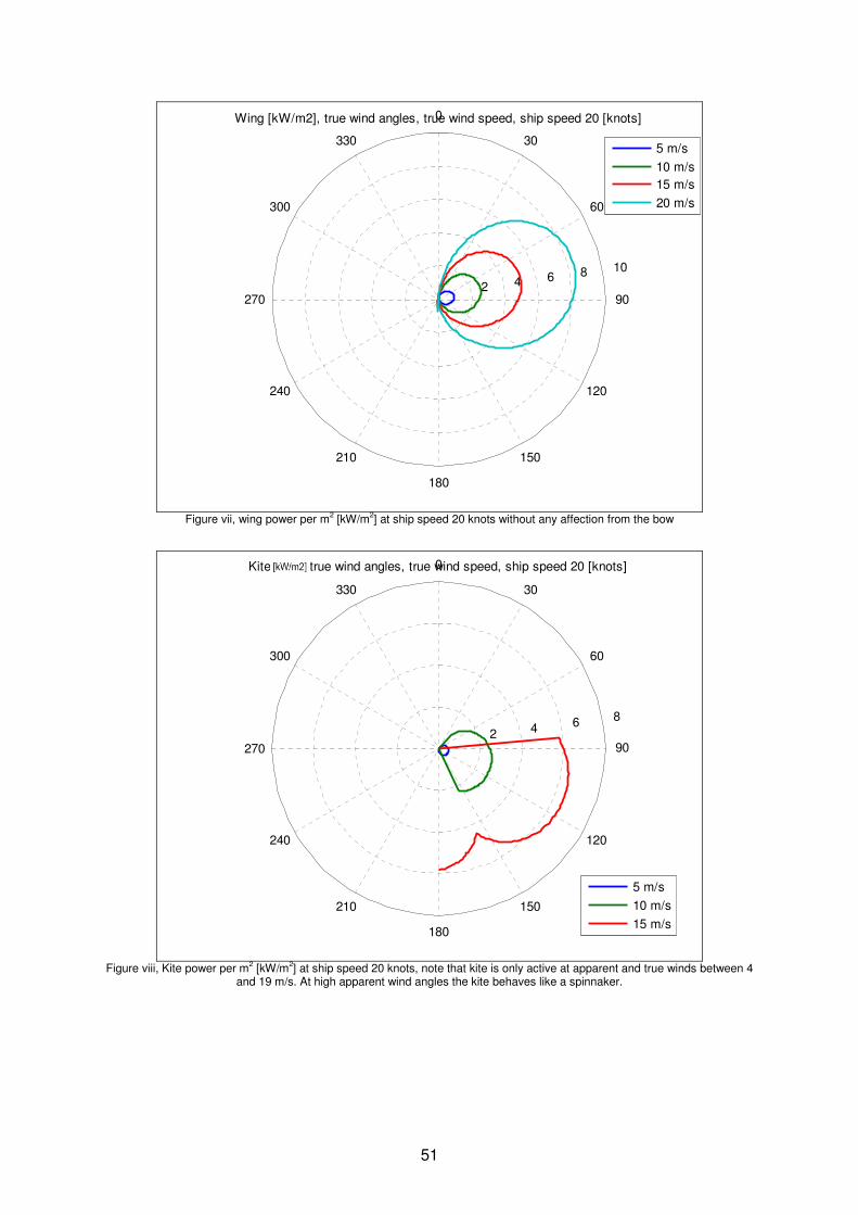
51

2 4 6 8 10

30

210

60

240

90270

120

300

150

330

180

0Wing [kW/m2], true wind angles, true wind speed, ship speed 20 [knots]

5 m/s

10 m/s

15 m/s

20 m/s

Figure vii, wing power per m2 [kW/m2] at ship speed 20 knots without any affection from the bow

2 4 6 8

30

210

60

240

90270

120

300

150

330

180


5 m/s

10 m/s

15 m/s

Figure viii, Kite power per m2 [kW/m2] at ship speed 20 knots, note that kite is only active at apparent and true winds between 4

and 19 m/s. At high apparent wind angles the kite behaves like a spinnaker.

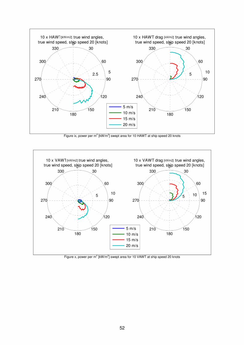
52

2.5 5

30

210

60

240

90270

120

300

150

330

180

0


5 10

30

210

60

240

90270

120

300

150

330

180

0


5 m/s

10 m/s

15 m/s

20 m/s

Figure ix, power per m2 [kW/m2] swept area for 10 HAWT at ship speed 20 knots

5 10 15

30

210

60

240

90270

120

300

150

330

180

0

10 x VAWT drag [kW], true wind angles, true wind speed, ship speed 20 [knots]

5 10

30

210

60

240

90270

120

300

150

330

180

0


5 m/s

10 m/s

15 m/s

20 m/s

Figure x, power per m2 [kW/m2] swept area for 10 VAWT at ship speed 20 knots

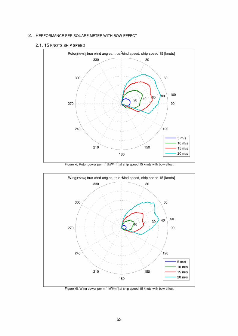
53

2. PERFORMANCE PER SQUARE METER WITH BOW EFFECT


20 40 60 80 100

30

210

60

240

90270

120

300

150

330

180

0Rotor [kW], true wind angles, true wind speed, ship speed 15 [knots]

5 m/s

10 m/s

15 m/s

20 m/s

Figure xi, Rotor power per m2 [kW/m2] at ship speed 15 knots with bow effect.

10 20 30 40 50

30

210

60

240

90270

120

300

150

330

180

0Wing [kW], true wind angles, true wind speed, ship speed 15 [knots]

5 m/s

10 m/s

15 m/s

20 m/s

Figure xii, Wing power per m2 [kW/m2] at ship speed 15 knots with bow effect.

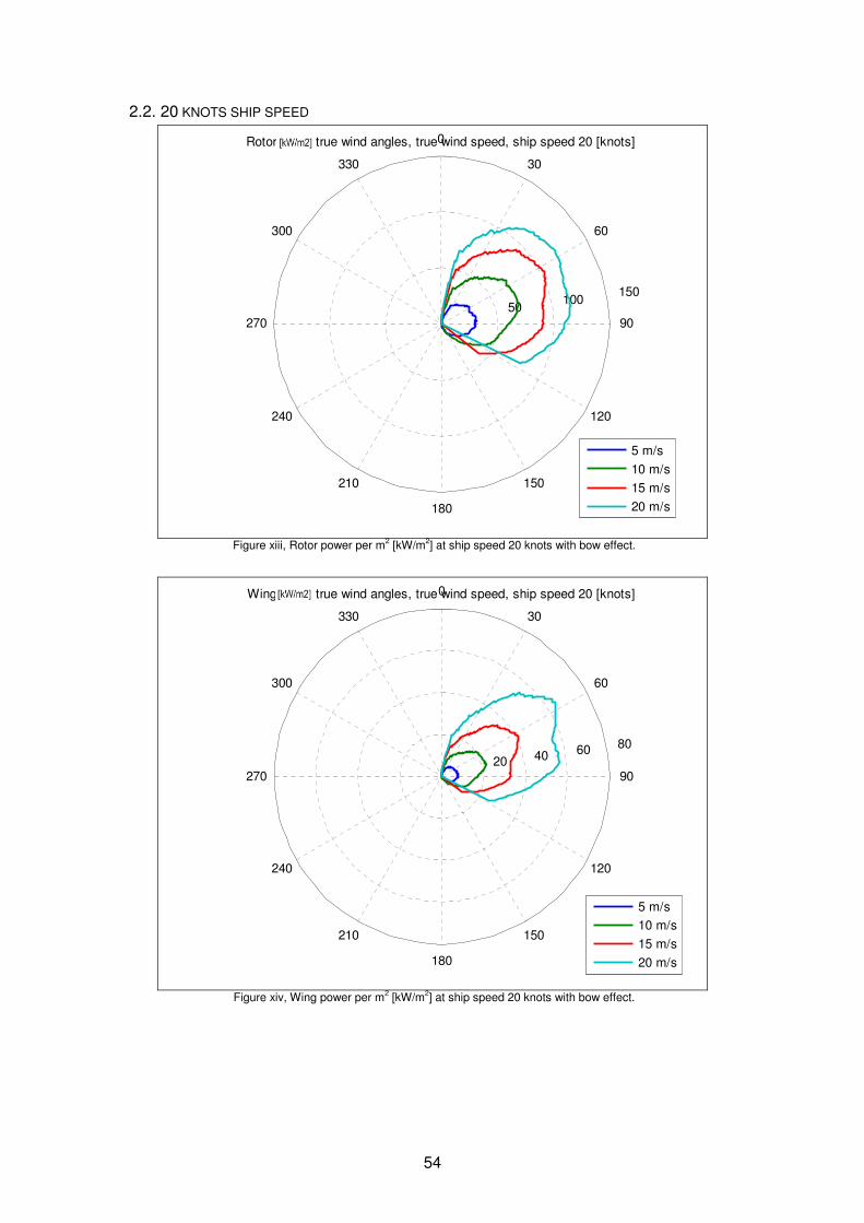
54


50 100

150

30

210

60

240

90270

120

300

150

330

180


5 m/s

10 m/s

15 m/s

20 m/s

Figure xiii, Rotor power per m2 [kW/m2] at ship speed 20 knots with bow effect.

20 40 60 80

30

210

60

240

90270

120

300

150

330

180


5 m/s

10 m/s

15 m/s

20 m/s

Figure xiv, Wing power per m2 [kW/m2] at ship speed 20 knots with bow effect.

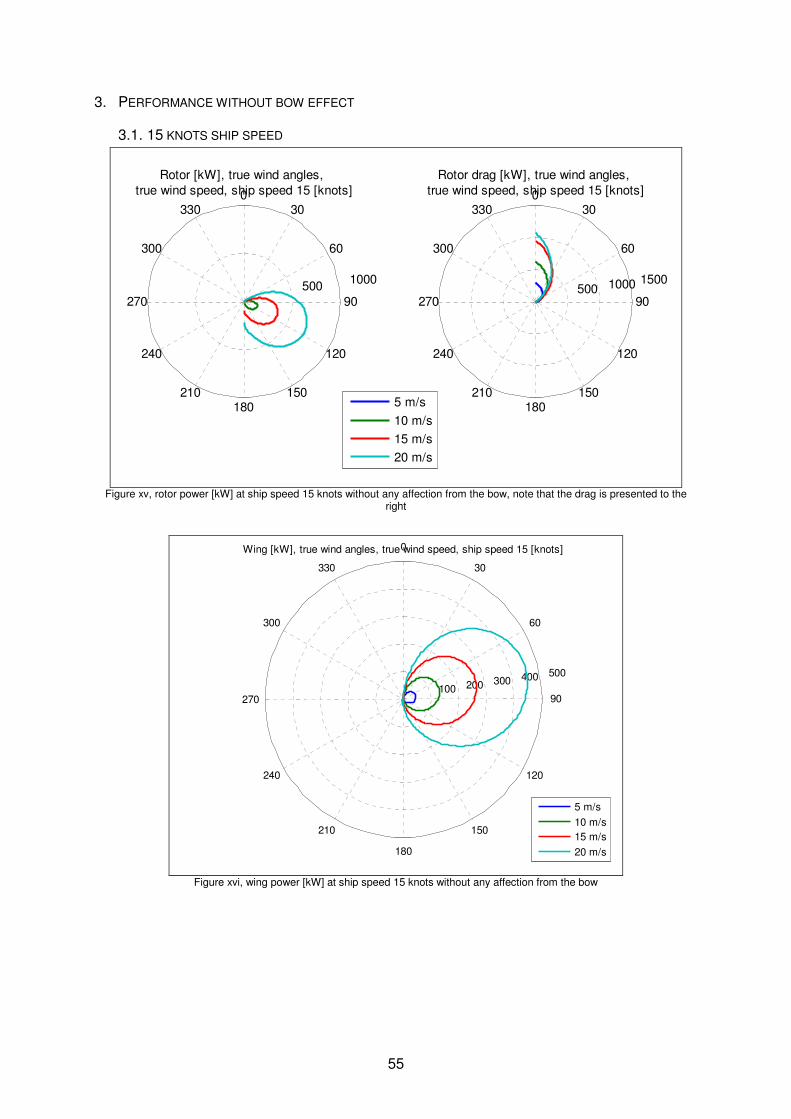
55

3. PERFORMANCE WITHOUT BOW EFFECT


500 1000

30

210

60

240

90270

120

300

150

330

180

0


500 1000 1500

30

210

60

240

90270

120

300

150

330

180

0


5 m/s

10 m/s

15 m/s

20 m/s

Figure xv, rotor power [kW] at ship speed 15 knots without any affection from the bow, note that the drag is presented to the

right

100 200 300 400 500

30

210

60

240

90270

120

300

150

330

180


5 m/s

10 m/s

15 m/s

20 m/s

Figure xvi, wing power [kW] at ship speed 15 knots without any affection from the bow

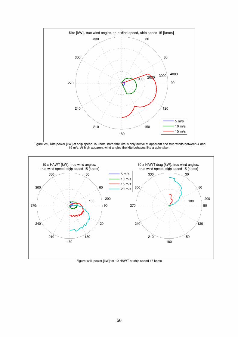
56

1000 2000 3000 4000

30

210

60

240

90270

120

300

150

330

180


5 m/s

10 m/s

15 m/s

Figure xvii, Kite power [kW] at ship speed 15 knots, note that kite is only active at apparent and true winds between 4 and

19 m/s. At high apparent wind angles the kite behaves like a spinnaker.

100 200

30

210

60

240

90270

120

300

150

330

180

0


5 m/s

10 m/s

15 m/s

20 m/s

100 200

30

210

60

240

90270

120

300

150

330

180

0


Figure xviii, power [kW] for 10 HAWT at ship speed 15 knots

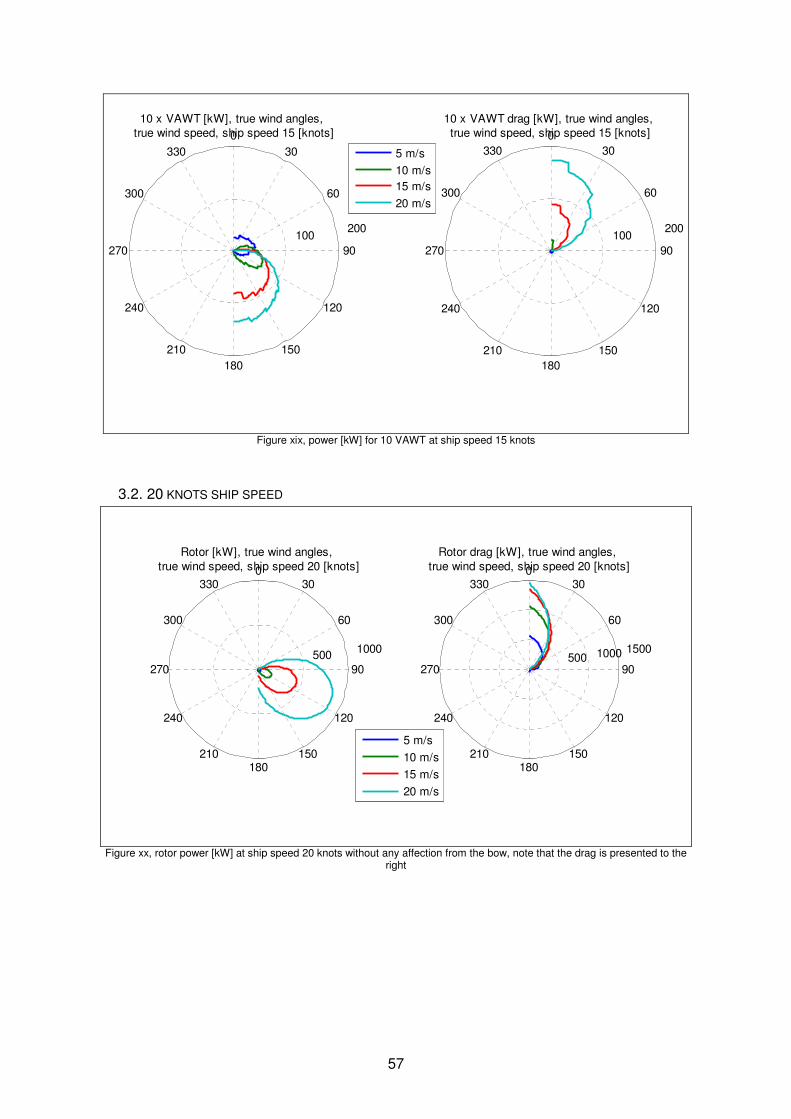
57

100 200

30

210

60

240

90270

120

300

150

330

180

0


5 m/s

10 m/s

15 m/s

20 m/s

100 200

30

210

60

240

90270

120

300

150

330

180

0


Figure xix, power [kW] for 10 VAWT at ship speed 15 knots


500 1000

30

210

60

240

90270

120

300

150

330

180

0


500 1000 1500

30

210

60

240

90270

120

300

150

330

180

0


5 m/s

10 m/s

15 m/s

20 m/s

Figure xx, rotor power [kW] at ship speed 20 knots without any affection from the bow, note that the drag is presented to the

right

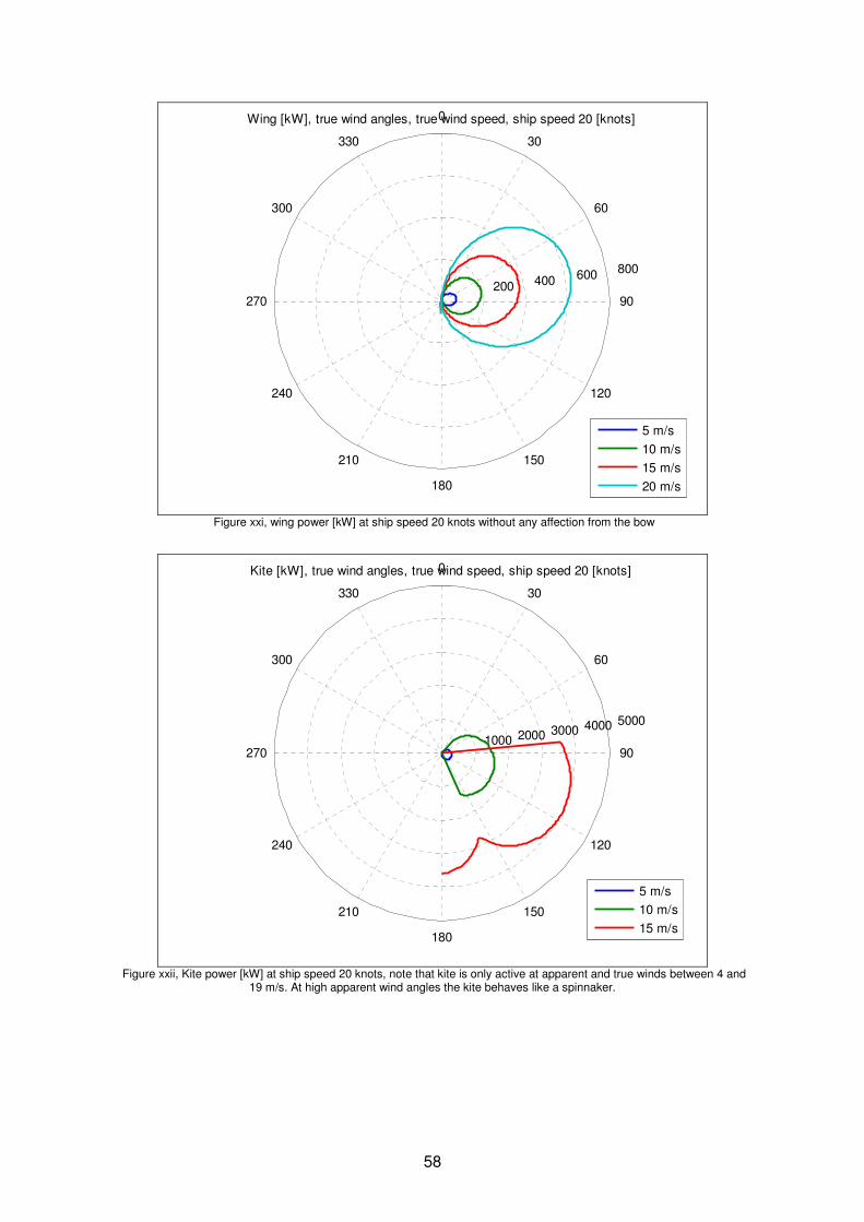
58

200 400 600 800

30

210

60

240

90270

120

300

150

330

180


5 m/s

10 m/s

15 m/s

20 m/s

Figure xxi, wing power [kW] at ship speed 20 knots without any affection from the bow

1000 2000 3000 4000 5000

30

210

60

240

90270

120

300

150

330

180


5 m/s

10 m/s

15 m/s

Figure xxii, Kite power [kW] at ship speed 20 knots, note that kite is only active at apparent and true winds between 4 and

19 m/s. At high apparent wind angles the kite behaves like a spinnaker.

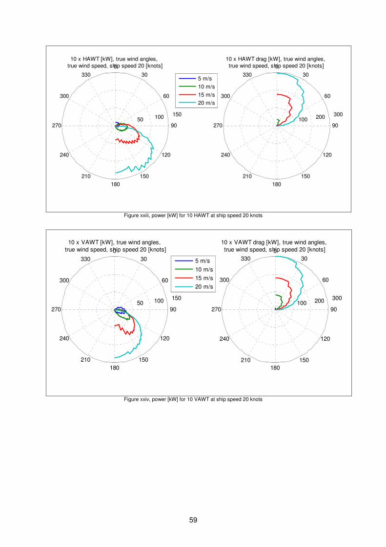
59

50 100 150

30

210

60

240

90270

120

300

150

330

180

0


100 200 300

30

210

60

240

90270

120

300

150

330

180

0


5 m/s

10 m/s

15 m/s

20 m/s

Figure xxiii, power [kW] for 10 HAWT at ship speed 20 knots

50 100 150

30

210

60

240

90270

120

300

150

330

180

0


100 200 300

30

210

60

240

90270

120

300

150

330

180

0


5 m/s

10 m/s

15 m/s

20 m/s

Figure xxiv, power [kW] for 10 VAWT at ship speed 20 knots

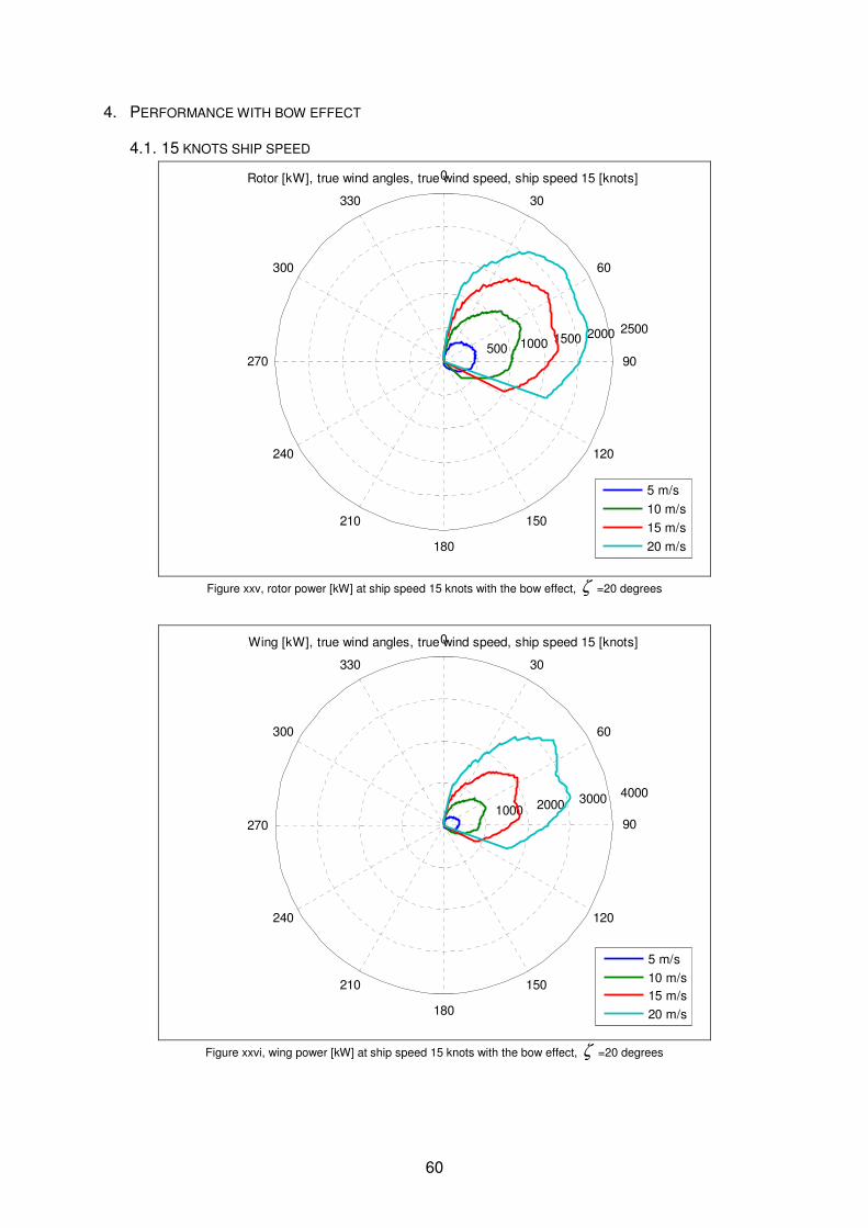
60

4. PERFORMANCE WITH BOW EFFECT


500 1000 1500 2000 2500

30

210

60

240

90270

120

300

150

330

180


5 m/s

10 m/s

15 m/s

20 m/s

Figure xxv, rotor power [kW] at ship speed 15 knots with the bow effect, ζ =20 degrees

1000 2000 3000 4000

30

210

60

240

90270

120

300

150

330

180


5 m/s

10 m/s

15 m/s

20 m/s

Figure xxvi, wing power [kW] at ship speed 15 knots with the bow effect, ζ =20 degrees

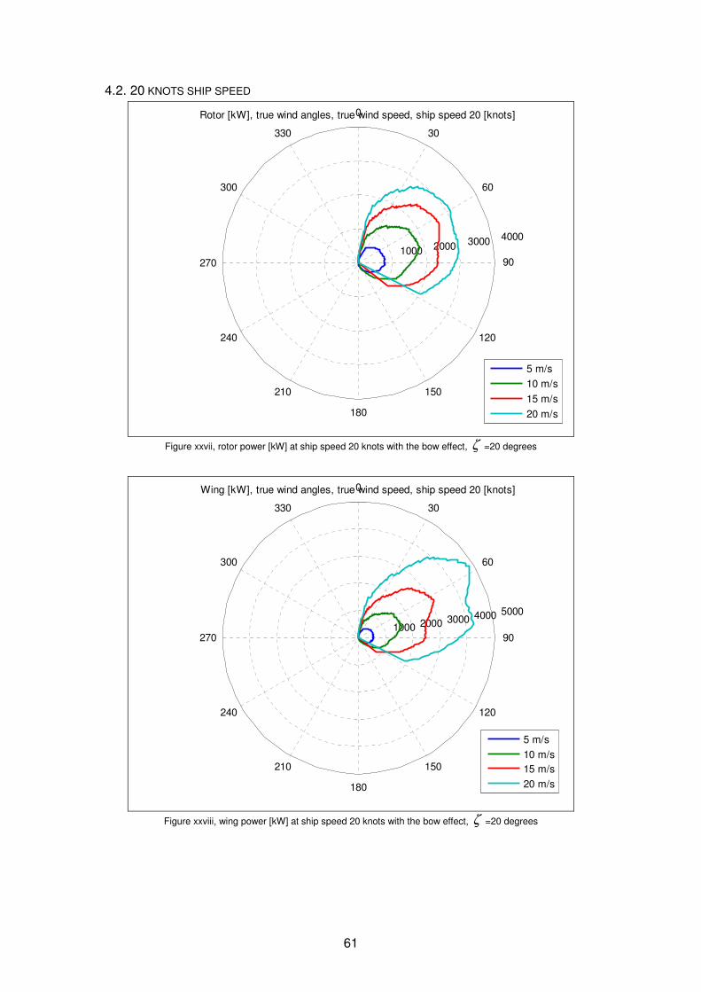
61


1000 2000 3000 4000

30

210

60

240

90270

120

300

150

330

180


5 m/s

10 m/s

15 m/s

20 m/s

Figure xxvii, rotor power [kW] at ship speed 20 knots with the bow effect, ζ =20 degrees

1000 2000 3000 4000 5000

30

210

60

240

90270

120

300

150

330

180


5 m/s

10 m/s

15 m/s

20 m/s

Figure xxviii, wing power [kW] at ship speed 20 knots with the bow effect, ζ =20 degrees

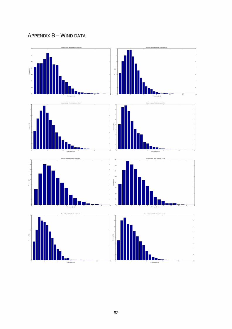
62

APPENDIX B – WIND DATA

0 5 10 15 20 250

2

4

6

8

10

12

14

Occura

nce [

%]

Wind speed [m/s]

True wind speed, World wide route in January

0 5 10 15 20 25 300

2

4

6

8

10

12

14

Occura

nce [

%]

Wind speed [m/s]

True wind speed, World wide route in February

0 5 10 15 20 250

2

4

6

8

10

12

14

16

Occura

nce [

%]

Wind speed [m/s]

True wind speed, World wide route in March

0 5 10 15 20 250

2

4

6

8

10

12

14

16

18

Occura

nce [

%]

Wind speed [m/s]

True wind speed, World wide route in April

0 2 4 6 8 10 12 14 16 180

2

4

6

8

10

12

14

16

18

Occura

nce [

%]

Wind speed [m/s]

True wind speed, World wide route in May

0 2 4 6 8 10 12 14 16 18 200

2

4

6

8

10

12

14

16

Occura

nce [

%]

Wind speed [m/s]

True wind speed, World wide route in June

0 5 10 15 20 25 300

5

10

15

Occura

nce [

%]

Wind speed [m/s]

True wind speed, World wide route in July

0 5 10 15 20 250

2

4

6

8

10

12

14

16

Occura

nce [

%]

Wind speed [m/s]

True wind speed, World wide route in August

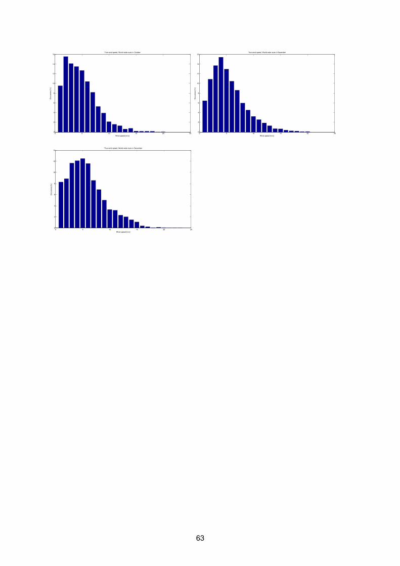
63

0 5 10 15 20 250

2

4

6

8

10

12

14

16

Occura

nce [

%]

Wind speed [m/s]

True wind speed, World wide route in October

0 5 10 15 20 250

2

4

6

8

10

12

14

16

Occura

nce [

%]

Wind speed [m/s]

True wind speed, World wide route in November

0 5 10 15 20 250

2

4

6

8

10

12

14

Occura

nce [

%]

Wind speed [m/s]

True wind speed, World wide route in December

64

REFERENCES 1. Tupper, Rawson. Basic ship theory - Fifth edition. Woburn : Butterworth-Heinemann, 2001. ISBN 0 7506 5398 1. 2. Tolle, Martin. Shiptracker.com. [Online] 27 January 2009. http://images.vesseltracker.com/images/vessels/midres/86256.jpg. 3. Schentzle, P. Estimation of wind potential. s.l. : Journal of wind engineering and industrial aerodynamics, 1985. 4. Massey, B:S. Mechanics of fluids (sixth edition). Padstow, Great Britain : Chapman & Hall, 1997. ISBN 0 412 34280 4. 5. Kuttenkeuler, Jakob. Surface ship controllability. Stockholm : KTH, Center for Naval Architecture, 2006. 6. Kuttenkeuler, Jakob. Segling - så funkar det. Stockholm : KTH - Center for Naval Architecture, 2007. 7. Hanson, T.F. Sail assist and the Spins'l. 1986. 8. Gernez, Etienne. DNV. 27 January 2009. 9. Gatenfjord, Göran. GGRail. 8 October 2008. 10. Flettner, A. Mein weg zum rotor. Leipzig : Köhler & Amelang, 1926. 11. Eliasson, Lars Larsson & Rolf. Principles of yacht design. Midsomer Norton : Adlard Coles Nautical, 2002. ISBN 0-7136-5181-4. 12. Carbonaro, M. Flow visualizations. Rhode Saint Genèse : von Karman Institute, 1994. 13. Bergeson, Lloyd and Greenwald, C. Kent. Sail Assist Development 1979-1985. Amsterdam : Elsevier Science Publishers, 1985. 19 (1985) 45-114. 14. Andersson, J.D. Introduction to flight. Third edition. s.l. : McGraw-Hill, Aerospace Science series, 1989. ISBN 0-07-100496-3. 15. International Energy Agency. World Energy Outlook 2008. 2008. 16. DSME, Daewoo shipbuilding and marine engineering co.ltd. Trim & Stability booklet, H.NO 4445. 2007. 17. Skysails. Technology information. Hamburg : Skysails, 2008. 18. Quiet Revolution. [Online] 2008. http://www.quietrevolution.co.uk/faq_qr5.htm#qr3. 19. New Scientist. [Online] 2009. http://www.newscientist.com/data/images/archive/2488/24881601.jpg. 20. Knud E. Hansen; Bloch, Martin Rosander and Jens O.V. Modern Windships. Copenhagen : Knud E Hansen, 2000. 21. Oklahoma state university; Fluid mechanics . Lecture notes Chapter 9 Lecture 4. 2008. ENGSC 3233. 22. Martin Hepperle. Javafoil. [Online] 2 5 2007. [Cited: 21 1 2009.] www.mh-aerotools.de/airfoils/javafoil.htm. 23. e24. [Online] 2009. http://bors.e24.se/bors24.se/site/commodity/commodity_detail.page?magic=(cc%20(detail%20(tsid%20130455)%20(graph%20(period%205Y)%20(from%20null)%20(to%20null)))). 24. Enercon. Christening and launch of “E-Ship 1” in Kiel. Aurich : Enercon, 2008. 25. Bergey. BWC Excel 10kW Class wind turbine. [Online] [Cited: 12 October 2008.] www.bergey.com/Products/Excel.Spec.Frt.pdf. 26. Danish wind industry association. Betz' law. [Online] [Cited: 22 Januari 2009.] www.windpower.org/en/tour/wres/betz.htm.

wind assisted propulsion for pure car and truck carriers

Documents