wind farms impact on radar aviation...
TRANSCRIPT

WIND FARMS IMPACT ON RADAR AVIATIONINTERESTS - FINAL REPORT
FES W/14/00614/00/REPDTI PUB URN 03/1294
The work described in this report was carried out undercontract as part of the DTI Sustainable EnergyProgrammes. The views and judgements expressed in thisreport are those of the contractor and do not necessarilyreflect those of the DTI.
September 2003
Contractor QinetiQ
Prepared by Gavin J Poupart
First published 2003© Crown copyright 2003

(ii)
This page is intentionally blank

(iii)
EXECUTIVE SUMMARY
Background
The Department of Trade and Industry (DTI) of the UK Government is committed to reducingcarbon emissions and revising the UK energy infrastructure. As such, increased renewableenergy generation is seen as a potential significant contributor to realising this vision. The UK’swind resource is significant and with the technology currently available, the UK has the potentialto harness a significant proportion of the UK’s energy requirements from this renewableresource.
The process of obtaining planning permission to build a wind farm involves manyconsiderations, including consultation with various aviation stakeholders, both civil and military.These parties may raise objections for a variety of reasons. A known source of objection is thatthe wind farm may appear on the display of air traffic control radar. Decisions made regardingthe likely impact that a wind farm may have upon radar operations are currently based uponassumptions. The electromagnetic interactions between a wind turbine and a radar signal arecomplex and there is currently limited understanding in this area and no accepted method forquantifying this potential impact.
A conflict of interest currently exists between the desire to encourage wind farm development asa renewable energy source and the desire to maintain the operational safety of air traffic. Thepractical manifestation of this conflict is that the UK has seen objections against a significantproportion of proposed wind farms on the grounds of aviation safety. This situation is obviouslyunsatisfactory to the wind energy industry. Often developers commit to the costs of siteassessments that are subsequently refused permission, are subjected to planning delays or aresignificantly constrained regarding potential areas for development if they are to avoid thispotential conflict.
Conversely, the current limited knowledge base and technical complexity of this subject areadoes not aid the aviation stakeholders when making assessments of the potential impact of windfarms upon aviation operational safety. The aviation stakeholders are often unable to provideclear and grounded comment as to whether a particular proposed wind farm presents a safetyissue or what would be needed to mitigate and achieve the safety confidence required. The DTIhas tackled this issue, in part, by commissioning this project to provide a detailed understandingof the interaction between wind farms and radar systems. It is anticipated that this study willprovide input into the revision of the “Wind Energy and Aviation Interests interim guidelines”ref. ETSU W/14/00626/REP for the siting of wind farms.
Objectives
The main objectives of the study were as follows:
• Determine the effects of siting wind turbines adjacent to primary air traffic controlradar;
• Provide the information required for the generation of guidelines by civil, militaryand wind farm developer stakeholders;
• Determine the extent to which detailed design of wind turbines influences theireffects on radar systems;

(iv)
• Determine the extent to which the design of the radar processing influences theeffects of wind turbines on radar systems.
Methodology
As a mechanism to predict the Radar Cross Section (RCS) of wind turbines and understand theinteraction of radar energy and turbines, a computer model has been developed by exploitingQinetiQ’s stealth technology expertise. This model operates in a ‘super-computer’ environmentand is designed to predict and simulate the impact of wind farms upon the primary radar display.The model considers the affects of the radar propagation over the terrain between the radar andthe wind farm, the dynamic radar scattering from the wind farm and the processing in the radar.It can then display its results on a simulated radar display
The model has been validated through a full-scale trial and modelling process. Data have beencollected from a number of sources: a single operational Enercon E-66 turbine located atSwaffham in Norfolk using a mobile experimental radar station, high fidelity RCS measurementsof a scale model blade in a compact range chamber and from the radar display at RAF Marham(a radar having visibility of the Swaffham turbine).
The propagation code used as an input to the model was successfully validated by comparing itsoutput with a validated public domain propagation model. A number of references are providedagainst other QinetiQ work that have in the past validated the QinetiQ propagation model as partof Ministry of Defence programmes.
In addition to the trial at Swaffham, some radar display video data were collected from Prestwickof a nearby multiple turbine wind farm appearing on the radar display. A model simulation wasrun of this wind farm with the turbines in a ‘typical’ configuration. Results provided additionalconfidence in the model’s predictive ability.
In summary, a predictive computer model has been developed, validated against a single turbinescenario and has shown an accurate prediction capability. The reality is that most sites ofconcern will have multiple turbines, further model validation could be gained through a multipleturbine trial.
Stakeholder benefits
The experience gained and learning achieved during the development and validation of thepredictive computer model have been used to perform a sensitivity analysis (identification of thesensitivity of sub-elements of the radar and wind farm interaction) and to compile a list of thekey factors influencing the radar signature of wind turbines. Together, these have enabled us toprovide a much more detailed quantification of the complex interactions between wind turbinesand radar systems than was previously available.
The following points summarise some of the results of the project:
• The design of the tower and nacelle should have the smallest RCS signaturepossible. The RCS of the tower and nacelle can be effectively reduced thoughcareful shaping;
• Large turbines do not necessarily lead to large RCS (i.e. tower height does notgreatly affect RCS);

(v)
• Blade RCS returns can only be effectively controlled though the use of absorbingmaterials;
• For low probability of detection, but a large clutter return, set wind turbines suchthat they are mainly yawed close to ±90° from the radar direction;
• For high probability of detection, but a smaller area of clutter, set wind turbinessuch that they are mainly yawed close to 0° and 180° from radar direction;
It was noted that some of the RCS predictions used in the model are 4 to 6 dB lower than themeasurements, near RCS peaks. This is a result of two main factors:
Firstly blade reflectivity. The blades are not metallic and therefore, have to be assigned areflectivity in the modelling process. This has been estimated, and it appears from themeasurements that the blades are more reflective than expected.
Secondly, the predictions carried out do not model any returns resulting from multipleinteractions within the turbine structure. Given geometry that gives rise to paths back to the radarvia multiple bounce these returns can be very large. Without this mechanism the predictions willbe different from the measurement where strong multiple bounce returns are present.
To reduce this difference we must deal with both of these factors. The turbine blades need to bemodelled with a more realistic reflectivity and the multiple bounce calculations must be includedin the turbine calculations.
The model has the potential to be a valuable tool for the wind energy community and canprovide a validated route to:
• Generate the detailed data required for more sophisticated initial screening than iscurrently available;
• Support the development of mitigation and solutions, including: sitingoptimisation, control of wind turbine RCS and enhanced radar filters (able toremove the returns from wind turbines);

(vi)
This page is intentionally blank

(vii)
LIST OF CONTENTS
Executive summary iii
List of contents vii
1 Introduction 11.1 Project background 1
1.2 Radar cross-section 2
1.3 Objectives of work 2
1.4 Report structure 2
2 Key factors influencing the radar signature of wind turbines 52.1 Learning as potential inputs to the DTI guidelines 5
3 Computer model development 113.1 Benefits of the model 11
3.2 Model philosophy 11
3.3 Code structure 12
3.4 Functionality 12
3.5 Model limitations 14
4 RCS predictions of wind turbines 154.1 Reason for RCS predictions 154.2 Input information 15
4.3 CAD Creation 15
4.4 Data collected 17
4.5 Results and analysis 17
4.6 Summary 23
5 Radar measurements 255.1 Scale model measurements 25
5.2 RCS prediction validation with a scale model blade 27
5.3 Trial planning 27
5.4 Swaffham trial 28
5.5 Swaffham results 30
5.6 Wind farm trial 34
6 Validation of the computer model 356.1 Validation philosophy 35

(viii)
6.2 RCS validation 35
6.3 Spectral content validation 43
6.4 Propagation validation 46
6.5 WHIRL validation 48
6.6 Summary 54
7 Parameter sensitivity 577.1 Current parameters 57
7.2 Further parameters 57
7.3 Detailed tower sensitivity study 59
7.4 Detailed nacelle sensitivity study 63
7.5 Detailed blade sensitivity study 66
7.6 Summary 74
8 Conclusions 758.1 Overview 75
8.2 RCS Predictions 75
8.3 Computer model development 76
8.4 Radar measurements 76
8.5 Validation of WHIRL 76
8.6 Key factors influencing the radar signature of wind turbines 78
8.7 Summary 79
9 Recommendations 81
10 Acknowledgements 83
11 List of abbreviations 85
A RCS modelling of wind turbines A-1A.1 Approximations in CAD models A-1
A.2 Main Enercon turbine dimensions A-2
A.3 Details of data collection technique A-2
A.4 Effects of internal structure A-2
A.5 Further results A-5
B Detailed model description B-1B.1 WHIRL COM B-1
B.2 WHIRL-DIS: Simulated radar display B-4
B.3 Ocellus: RCS computation B-8

(ix)
B.4 NEMESIS: propagation calculation B-10
B.5 Shadowing B-12
C Outline wind turbine trials plan C-1C.1 Introduction C-1
C.2 Concept of necessary trials data C-1
C.3 PPI Video Collection C-2
C.4 RCS and raw radar data collection C-4
C.5 Summary of trials C-6
D Radar measurement details D-1D.1 MPR site D-1
D.2 MPR parameters D-1
D.3 Radar calibration and performance checks D-1
D.4 Blade position sensor D-2
D.5 Full results D-4
E Circular polarisation E-1
F Identification of UK wind farms within line-of-sight of primary radar F-1F.1 QinetiQ introduction F-1
F.2 Emrad Introduction F-1
F.3 Wind Farms F-2
F.4 UK Radar Installations F-2
F.5 Description of the Database F-3
G Independent review of WHIRL G-1G.1 QinetiQ introduction G-1
G.2 EMRAD introduction G-1
G.3 Ocellus G-2
G.4 NEMESIS G-4
G.5 Wind Farms Having Interaction at Radar Locations (WHIRL) G-5
G.6 Investigation of the Radar Cross-Section of a simple wind turbine blade section G-8
G.7 Overall Conclusions G-16
G.8 Mathmatics appendix G-19
References G-21

(x)
This page is intentionally blank

Page 1 of 86
1 INTRODUCTION
1.1 Project background
1.1.1 The Department of Trade and Industry of the UK Government has a policy ofencouraging the development of renewable energy sources. One such renewable energysource is the power available from the wind. With the position of the UK on the edge ofthe continent of Europe, wind energy is particularly plentiful, so that wind is a promisingrenewable energy source for the UK.
1.1.2 The process of obtaining planning permission to erect a wind turbine or a wind farm (agroup of wind turbines built on the same site) involves many considerations, includingconsultation with various aviation interests, both civil and military. These parties mayraise objections to a proposed wind turbine for a variety of reasons. One common sourceof objection from the Royal Air Force is that the wind turbine, being a tall object (70 to100 metres or more), is a threat to the safety of low-flying military aircraft on trainingflights. Another source of objections is that the wind turbine will appear as an echo onthe display of radar used in air traffic control (ATC). This echo distracts the air trafficcontroller from the aircraft echoes which are his main interest, and can reduce theeffectiveness of the radar by masking genuine aircraft returns. This is considered as athreat to the safety of air traffic, both civil and military.
1.1.3 There is, thus, a conflict of interest between the desire to encourage wind farmdevelopment as a renewable energy source, and the desire to maintain the safety of airtraffic. In practice, a large fraction of proposed wind farms have objections lodgedagainst them on grounds of aviation safety. This situation is unsatisfactory to the windenergy industry, as it involves them in the expense of preparing cases for wind farmdevelopment at sites that are subsequently refused permission, and considerably restrictsthe areas available for wind farm development.
1.1.4 The Department of Trade and Industry, contracting via Future Energy Solutions (FES) atHarwell has set up a working party under the title “Wind energy, defence and civilaviation interests”. This provides a forum for representatives of the wind energy industryto meet with civil and military aviation authorities, and discuss these issues. Examples ofwind farms in the vicinity of ATC radar exist in the UK. In some cases, problems havebeen reported and documented.
1.1.5 Cases are known where the presence of a wind farm adjacent to an airport is causingproblems for the ATC of the airport. On the other hand, cases are also known where awind turbine close to an airfield causes little or no problem to the airfield ATC. Thereasons for this apparent inconsistency are not well understood.
1.1.6 This lack of understanding makes it hard for the aviation safety authorities to give clearand well-founded decisions on whether a particular proposed wind farm presents a safetyissue or not.
1.1.7 The Department of Trade and Industry commissioned this study to clarify the interactionof wind turbines and radar systems, and to provide input into the production of guidelinesfor the siting of wind turbines near radar systems.

Page 2 of 86
1.2 Radar cross-section
1.2.1 Throughout this report we will be using the term, radar cross-section (RCS). For readersunfamiliar with this term the following paragraphs are a description of its meaning.
1.2.2 An essential element in considering the detection of a wind turbine by a radar is thestrength of the radar reflection from the turbine. This is measured by its RCS, which is anarea, usually measured in square metres. It can have a wide range of values, and is oftenquoted in decibel square-metres (dBsm), which is a logarithmic measure. An RCS of0dBsm means 1 square metre, every 3dB increase doubles the value in square metres,and each 10dB added means that the RCS is multiplied by 10.
1.2.3 In the special case of a large metal sphere, the RCS is equal to the area of the geometricalcross-section. For other targets it can be much greater than the geometrical area (e.g. aflat plate viewed at right angles, or the corner reflector used on buoys and small boats).In yet other targets it can be much smaller than the geometrical area (e.g. a stealthaircraft).
1.3 Objectives of work
1.3.1 The main objectives of the work are as follows:
• Provide information for the generation of guidelines for the siting of wind turbinesnear radar systems;
• Determine the effects of siting wind turbines adjacent to radar systems;• Determine the extent to which the detailed design of the turbines influences their
effect on radar systems;• Determine the extent to which the radar processing influences the effects of wind
turbines on radar systems.
1.3.2 To achieve these aims QinetiQ set out to complete the following tasks:
• Develop a computer model to simulate the effects of wind turbines on radarsystems;
• Carry out radar cross-section (RCS) predictions of four wind turbine designs andanalyse their radar signatures;
• Plan field trials to validate the predictions and computer model;• Validate the predictions and model against the data collected in the field trials
1.3.3 After planning the field trials QinetiQ was also instructed to carry out these trials and thisis also reported on here.
1.4 Report structure
1.4.1 The main report is split into sections, each containing details of one of the tasks carriedout. Section 2 pulls together findings gained from the completion of this work into keyfactors influencing the radar signature of wind turbines, which should help thedevelopment of siting guidelines.

Page 3 of 86
1.4.2 Section 3 reports on the development of a computer model to simulate the effects of windturbines on radar systems. This model is developed using QinetiQ experience in radarscattering and radar propagation to allow the effects of a turbine on a primary radardisplay to be simulated.
1.4.3 Section 4 reports on RCS predictions carried out on wind turbines. The RCS of an objectis a measure of how much energy is returned to the radar, and hence is critical inunderstanding, and simulating the effects of a wind turbine on radar. The predictions aredone using QinetiQ prediction codes developed from 20 years of research in the UKstealth programme.
1.4.4 Section 5 contains the details and results of the radar measurements that have been madeto validate the predictions and the computer model described in section 2. Thesemeasurements have been carried out on a scale model turbine blade in a QinetiQmeasurement facility and of a real turbine using a QinetiQ mobile experimentation radar.
1.4.5 Section 6 explains the validation process and the results from this exercise. Thevalidation uses all the data collected and explained in sections 3 and 4 to validate thecomputer model described in section 2. The model has been run to reproduce measuredscenarios and the resulting output compared to the measured result.
1.4.6 Section 7 identifies the key parameters that influence the effects a turbine will have on aradar system. Examples would be the parameters which affect the RCS, and hence thereturning power to the radar and radar settings and filters.
1.4.7 Section 8 contains the conclusions from the report, summarising all of the findings fromthe previous sections.
1.4.8 Section 9 describes the recommendations resulting from this study.
1.4.9 The following sections in the main body of the report concentrate on the results andfindings of the study. All the technical detail and mathematics are presented inappendices at the back of the report and are referenced from the main text.
1.4.10 Appendix A includes details of how the modelling of the wind turbines was carried out,and reasoning for the simplifications made. It also includes results from the predictionscarried out.
1.4.11 Appendix B includes a detailed description of the computer model, fully describing thefunctionality of each of the model parts. It also includes a section on the mathematics ofradar shadowing caused by turbines.
1.4.12 Appendix C is the outline trials plan that was generated early in the project to define thetrials to be carry out.
1.4.13 Appendix D includes details of the radar trials carried out, including calibration andinstrumentation issues. It also includes more processed measurement results.
1.4.14 Appendix E includes a discussion of the issues surrounding circular polarisation andshows that the RCS prediction techniques used in this work can be applied to circularpolarisation problems.

Page 4 of 86
1.4.15 Appendix F details the work carried out by the subcontractor EMRAD in creating adatabase of radar sites within line of site (LoS) of wind farms in the UK.
1.4.16 Appendix G contains a review of the QinetiQ computer model by the subcontractorEMRAD, explaining their views on the work carried out and the validity of the model.

Page 5 of 86
2 KEY FACTORS INFLUENCING THE RADAR SIGNATURE OFWIND TURBINES
2.1 Learning as potential inputs to the DTI guidelines
2.1.1 In order to detail the relevant input sections for the DTI guidelines, they are identifiedbelow under the following headings for clarity; Wind turbine, Wind farm, Terrain, andRadar.
2.1.2 Wind turbine
2.1.2.1 Design (Shape). A typical wind turbine is made up of three main components, the tower,the nacelle, and the rotor. We have carried out a study of the effects of shape on the RCSof these components (see section 7). We consider each of the turbine components andpresent the key factors influencing the radar signature.
2.1.2.2 The wind turbine tower is a constant return that should be minimised to aid the radarfiltering of the turbine. Radar processing can suppress stationary objects, but if the RCSis too high then the object will still appear as clutter on the PPI display. It should benoted that although the tower is essentially stationary it does vibrate and sway undernormal operation and this may have an effect on the radar filtering.
2.1.2.3 For a tapered cylindrical tower increasing the taper angle will greatly reduce the towerRCS (e.g. Enercon tower RCS is ≈100m2. Increasing taper angle by 2° reduces RCS to≈10m2). Over the range of likely tower sizes the diameter and height of the tower onlyhave a small effect on the tower scattering. As the tower does not move, squashing thetower into an oval cross-section and pointing the narrow cross section at the radar canfurther reduce its RCS. This is only effective if there is one illuminating radar system asthe RCS will be lower only when looking at the narrow tower cross-section (for detailssee section 7.3). The tower of a wind turbine will bend under normal operation due towind load and thermal heating. These effects are likely to be big enough to significantlyeffect the tower RCS, and need to be taken into consideration when designing a tower forRCS control.
2.1.2.4 Unlike the tower the turbine nacelle RCS is a function of the turbine yaw angle. It rotatesonly slowly with respect to the radar, hence will be suppressed by radar filters. As withthe tower it is still important to keep this return to a minimum to give the radar the bestchance of filtering the turbine return.
2.1.2.5 Curved surface nacelles send energy in all directions, giving a less variable but high RCSwith changing yaw angle. Flat panel nacelles create a variable RCS return with very highspikes and regions of low returns as the yaw is varied (e.g. the Enercon curved nacellevaries between 2m2 and 160m2, where as the Vestas flat panel nacelle varies between0.003m2 and 12,600m2). To create an all round low nacelle return flat panels angled awayfrom the radar (tilted up or down) should be used (e.g. the Vestas nacelle maximum canbe reduced from 12,600m2 to 50m2 with a 10° tilt angle. See section 7.4 for more details).
2.1.2.6 With current nacelle designs (rounded or flat panel) the yaw angles which give the lowestRCS are around ±45° and ±135° with the highest RCS occurring at 0°, ±90°, and 180°.

Page 6 of 86
2.1.2.7 The turbine rotor is very important in considering the effect of wind turbines on radar. Asit is spinning a proportion of the blades (depending on yaw angle and RPM) will betravelling fast enough to be unsuppressed by most radar stationary clutter filters. Hence,unless these returns are below the radar threshold then the turbine will appear as a targeton the radar PPI display.
2.1.2.8 The RCS of a turbine rotor changes rapidly as the blades rotate, and also vary as theturbine yaws and the blades pitch. From the data collected in this work on a number ofblade designs (see section 7.5 for details) it is clear that, during a single revolution of therotor, for any yaw angle a large RCS will be seen at some point. Shaping to control theRCS is only effective over a limited region of aspects. The same energy is being reflectedbut if we can concentrate it into a small number of directions this will leave regionswhere there is little backscatter of energy. As the blades will present most aspects to theradar at some point in time, shaping will have little effect on minimising the rotor RCSover any significant time period. The only real answer is to try and absorb some energythrough the use of materials.
2.1.2.9 Material. A study proposal from QinetiQ is under consideration by the DTI to investigatethe radar reflectivity of different wind turbine materials and if carried out will more fullyaddress this issue in due course.
2.1.2.10 However, it is safe to say that the materials used in the manufacture of a wind turbinewill affect the wind turbine’s RCS value. In particular, metals and other electricallyconducting materials, such as carbon fibre, are reflective to radar and, therefore, willcontribute to increasing the RCS signature. Where the material used has semitransparentproperties (such as wood or glassfibre) to radar, the internal structure of the wind turbinemay need to be considered.
2.1.2.11 Operation (Yaw). The wind turbine RCS varies with the Yaw i.e. with the relativeorientation of the wind turbine and the radar.
2.1.2.12 The components of the turbine that are a function of yaw are the nacelle and the rotor. Asalready discussed the nacelle RCS is minimised at ±45° and ±135° yaw angles, but asthis is likely to be suppressed by radar filters, it is not the key source of scattering as seenby the radar. So are there any preferable yaw angles for minimising the effect from theturbine rotor blades? We must take account of the stationary clutter filter which willaffect how the rotor appears to the radar as the yaw is varied. As the yaw moter movesthe rotor axis closer to facing the radar the relative speed of the blades towards and awayfrom the radar decreases and so the radar return from a greater proportion of the bladeslength is suppressed by the radar filters. The maximum speed of the blades in thedirection of the radar, and hence the least suppression of the blade RCS, occurs when therotor is facing 90° from the radar.
2.1.2.13 From our analysis we see that that from yaw angles around 0° and 180° (i.e. when theturbine is facing towards or away from the radar) the RCS of the blades are consistentlyhigh (around 100 to 1000m2) throughout a complete rotation (see section 7.5 for details).This means that whenever the radar looks at the turbine there is a high probability ofseeing a large signal and detecting the turbine. But this does not take account of the radarfilters which will be more effective at this yaw angle. The filter is likely to suppress alarge amount of the turbine return leaving just a small signal (i.e. a small region of PPIclutter) that is just detectable but with a high probability of detection. At the other
Page 7 of 86
extreme when the rotor is facing 90° from the radar (yaw of ±90°) the RCS of the turbineblades are very variable. When a blade edge is vertical (blade pointing up or down) avery large RCS is seen which is as large if not larger than the blade face return. But thisonly occurs for a short time during the blade rotation and for the rest of the time the RCSis low (below 1m2). Also as the blades are moving in the direction of the radar beam theradar filter will not suppress much of the returning energy for a vertical blade. This givesrise to a situation where the turbine will go undetected unless a vertical blade is observed,and if one is seen the resulting clutter on the PPI screen is large. The time periods in aturbine’s rotation when the RCS is high are short, and the probability of detection low,but when seen the resulting clutter will be large.
2.1.2.14 Blade Pitch. If a turbine has pitching blades then the effect of this pitching angle resultsin an adjustment to the yaw angle at which the situations described above occur. If theblades are pitched back by x degrees then the large RCS seen close to 0° and 180° yawdue to the blade faces will now occur at x° and 180+x°. Large pitch angles can createlarger clutter problems by moving the large RCS seen, when looking at the front or therear face of the blades, to a yaw angle where the radar filter is less effective (see section7.5 for details).
2.1.2.15 Blade Numbers. Whilst the current wind turbine is tending towards three-bladed systems,other blade configurations are feasible, the effects of which may be to vary the RCS. Thisrequires further investigation although it should be noted that the model described withinthis report can manage any blade configuration that the manufacturer’s may wish toconsider.
2.1.2.16 Rotation Speed. The rotational speed and the diameter of the turbine rotor determine thevelocity at the tip of the rotor. For a radar filter to suppress the whole blade, the tip speedof the blade in the direction of the radar must be less than the speed at which the radarfilter passes incoming radar returns unsuppressed. For a typical filter the suppressionbecomes less effective at around 50kph.
2.1.2.17 Lower rotational speeds for a given rotor diameter would allow more suppression tooccur, but given that typical rotor RPM are between 15 and 25, giving rise to tip speedsin excess of 160kph, high suppression over a wide range of yaw angles would requiremuch slower rotational speeds. For example, a maximum tip speed of 50kph for a 60mrotor would limit the RPM to 4.5. Small reductions in rotational speed will have littleeffect on the radar impact.
2.1.3 Wind farm
2.1.3.1 Range. Current procedures have put a lot of emphasis on the range of the wind farm fromthe radar. This has led to an impression that the further from the radar the farm is placedthe smaller the interference. The situation is not that simple. A greater range is onlybetter because it will increase the chances of intervening terrain and the earth’s curvatureobscuring the radar LoS to the turbines. Due to the magnitude of scattering from a windturbine, if the wind farm is within the operating range of the radar and LoS exists thenthe radar will receive clutter signals from the turbines.
2.1.3.2 Layout Spacing. Spacing of wind turbines within a wind farm is typically of the order ofa few hundreds of metres. The resolution of the radar in cross range is a function of thedistance between the radar and the wind farm and the radar beam width. The downrange

Page 8 of 86
resolution is dependant on the pulse width of the radar involved and is typically in therange of 50-300 metres.
2.1.3.3 If the spacing between the towers of the wind farm were smaller or equal to the crossrange and down range resolutions, then tracking of aircraft over the wind farm would bevery difficult. This is because radar will not resolve two targets that are within theresolution of the radar and will just appear as one large target. Conversely, if the windturbines were several resolution cells apart, then there is resolvable space between theturbines and a potential to see the crossing aircraft amongst the turbine returns.
2.1.3.4 Layout Geometry. It has yet to be established which wind farm layout is more acceptableand more research is needed to determine the optimal arrangement as far as radaroperators are concerned. However the following statements can be made regarding howvarious layout arrangements will appear to any radar system.
2.1.3.5 A grid layout will display as a regular pattern on the radar. This may prove easier for theradar operator to identify on the display.
2.1.3.6 A line of wind turbines running parallel to the radar’s boresight will tend to produce adeeper but narrow radar shadow due to the cumulative blocking effect of the line of windturbines. A line of wind turbines that is offset at an angle to the radar’s boresight willtend to produce a wider but less deep radar shadow as the angle increases. A line of windturbines perpendicular to the radar’s boresight will produce minimal radar shadow. Arandom layout, which in reality is more likely, will produce a combination of the aboveeffects. Which of these layouts is best will depend on what the radar coveragerequirements are at low level behind the wind farm.
2.1.3.7 In a circumstance where a single wind turbine in clear LoS to the radar is undetectedthen, assuming sufficiently wide spacing of wind turbines in wind farm, it is highly likelythat a wind farm of similar wind turbines would also be undetectable.
2.1.4 Terrain
2.1.4.1 Line of Sight between Radar and wind farm. As radar operate on a Line of Sight (LOS)basis, it is obvious that direct LOS between wind farm and radar should be avoidedwherever possible i.e. by using the intervening terrain to mask the wind farm from theradar. If there is a LOS and the radar is working effectively then any wind turbine willcause radar clutter.
2.1.4.2 Over the horizon effects. Wind farms can create a detectable radar return even when notin direct LoS of the radar. This is due to diffraction over the intervening ground betweenthe radar and wind farm. The level of detectability of the wind farm is dependant onfrequency of radar and the distance from the wind farm to the point of diffraction and thedistance below the LoS horizon where the wind farm is located.
2.1.4.3 Effect of wind turbine/wind farm on more distant objects. The diffraction effectsmentioned above, and the design of wind turbines, mean that wind turbines individuallycreate ‘radar shadows’. Any shadow that does exist behind wind turbine decreases inintensity with distance (e.g.) for a 3GHz radar, the shadow extends hundreds of metresbehind a typical wind turbine (see Annex B.5).

Page 9 of 86
2.1.5 Radar
2.1.5.1 Frequency. Frequency of radar systems varies but is generally in one of three bands:10GHz (3cm wavelength), 3GHz (10cm) and 1GHz (30cm). Higher frequency radarprovides greater resolution i.e. the individual radar tracks are smaller and easier todifferentiate. Hence for those radar with the highest frequencies, there is a smaller chanceof both an aircraft and a wind turbine being in the same radar resolution cell causingtrack merge.
2.1.5.2 Track Filtering. All radar contain filtering systems that are designed to extract outinformation that is of use for the particular radar purpose and to reject all otherinformation (perceived as clutter). As already discussed above, operating wind turbinesexhibit many of the characteristics associated with aircraft i.e. relatively large RCS with astrong Doppler shift. As current generation radar systems are not designed for theremoval, by filtering, of clutter from wind turbines, we have a situation where windturbines can cause clutter and false tracks on radar displays.

Page 10 of 86
This page is intentionally blank

Page 11 of 86
3 COMPUTER MODEL DEVELOPMENT
3.1 Benefits of the model
3.1.1 The benefit of this model is to allow the effects of any particular wind farm on aparticular radar to be accurately predicted. This can assist in the production of theregulatory guidelines by highlighting the important parameters and allowing theseparameters to be quickly modified and the effect on the radar observed.
3.2 Model philosophy
3.2.1 The purpose of this model is to investigate in detail what the effects of radar echoesreceived by radar from a wind turbine are, and to study the effects of the radar signalprocessing on these highly variable echoes. This will give an understanding of thecircumstances under which a turbine is visible to radar and when it is not visible. It alsoenables the examination of proposed means to distinguish wind turbine echoes fromother echoes, and then if possible prevent them from obscuring wanted targets on theradar operator's display.
3.2.2 The basic idea of the computation is to study the progress of each radar pulse transmittedduring a specified interval of time. During this interval the radar dish rotates, a (wanted)target aircraft moves across the scene, and blades rotate on one or more wind turbines.The magnitude of each received pulse is calculated, taking into account the antenna beampattern, the propagation from the antenna to the target aircraft and the turbines, and thevariable RCS of the aircraft and turbines. These returns are then passed through asimulation of representative radar signal processing, leading to a list of confirmed echodetections. These are then displayed on a plan-position indicator (PPI) display typical ofradar displays. A PPI is just a monitor on to which all the radar information is displayedfor the operator to interpret.
3.2.3 QinetiQ's software suite for studying and analysing the interactions of wind turbines withthe performance of radar systems is known as WHIRL.
3.2.4 The software has been designed in a modular way corresponding to each of the followingstages that require simulation. These stages are:
• Radar transmission of a pulse;• Propagation of pulse over terrain from radar to wind farm;• Scattering of pulse by wind farm;• Propagation of pulse over terrain from wind farm to radar;• Radar receives returning energy pulse;• Radar signal processing;• Radar display.

Page 12 of 86
3.2.5 WHIRL itself consists of two parts, and it uses output from two other programs tosimulate these processes:
• WHIRL-COM: simulates the radar signal processing;• WHIRL-DIS: simulates a radar PPI display, using radar echo information output by
WHIRL-COM;• Ocellus: computes the RCS, a measure of the energy scattered by the wind turbines
(feeds into WHIRL-COM);• NEMESIS: computes the propagation factor between the radar and the wind
turbines and back to the radar (feeds into WHIRL-COM).
3.2.6 This is described in more detail in the following sections.
3.3 Code structure
3.3.1 Figure 3-1 is a diagram of how all the code modules fit together.
Nemesis
Creates propagation patternfactor which takes into
account effects of terrainand elevation beam pattern
of radar
Ocellus
Run previously to collect allRCS data on turbines
WHIRL DIS
RCS Library
Propagation pattern factorLibrary
WHIRL COMMain computational function containing scenario set-up, radar
range equation, and radar processing
Figure 3-1; Diagram of how the QinetiQ software WHIRL fits together
3.4 Functionality
3.4.1 The functionality of each of the modules is briefly explained here. A more detailedexplanation is contained in appendix B.
3.4.2 WHIRL-COM
3.4.2.1 WHIRL-COM performs the computational work of simulating the reflection of radarsignals from a target aircraft and one or more turbines, and tracing the echoes throughappropriate radar signal processing.

Page 13 of 86
3.4.2.2 WHIRL-COM consists of four main sections:
• Graphical user interface, which allows the user to input data on the scenario to bemodelled, and controls the running of the subsequent computation;
• Calculation of the geometry of motion of an aircraft target, and rotation of turbineblades;
• Radar equation calculation, which takes into account the rotation of the radar beam,the propagation factor from radar to aircraft target and turbines, and the RCS as theaircraft target moves and the turbine blades rotate;
• Simulates radar data processing, including pulse integration, moving targetindication, and noise-related thresholding. Outputs the confirmed detections forinput to WHIRL-DIS.
3.4.2.3 WHIRL-COM can model any number of turbines in any position in the UK (other siteswould be possible given the relevant terrain data required). One aircraft target can beflown on a straight track across the display. Its start position, stop position and speed isset by the user. The code is currently set up to model a standard ATC primary radar, butall the radar parameters can be changed to suite different radar operations.
3.4.3 WHIRL-DIS
3.4.3.1 WHIRL-DIS is a program that simulates a radar operator's plan position indicator (PPI)display. It takes in the file from WHIRL-COM containing the accepted radar detections,and displays it in real time on the PPI display. This gives a visual indication of the effectsof the various signal processing options.
3.4.3.2 The program was kept separate from WHIRL-COM so that it could be run on a portablecomputer for demonstration purposes. The separation ensures that WHIRL-DIS can runfast enough to display its output in real time, and is not held up by any time consumingcalculations that are done in WHIRL-COM.
3.4.3.3 WHIRL-DIS does processing of its own: it accepts and displays the detections found inits input file. It contains additional thresholding with a user-adjustable range-dependentthreshold. This allows the user to see the effect of adjusting the threshold withoutrepeating the WHIRL-COM calculations.
3.4.3.4 When reading` an input file the user can select what threshold to set, and whether themoving target indicator (MTI) filter switch is on or off. Once a simulation is read in toWHIRL-DIS the user has a full range of viewing tools to enable the results to beevaluated. These are:
• Centre the simulation by mouse and keying in;• Zoom in and out by increments, mouse and keying in;• Variable display persistence of radar detections;• Start and stop simulation at will;• Move back and forth through simulation one second at a time;• Reset simulation.
3.4.3.5 A comprehensive description of WHIRL DIS is contained in Appendix B.2.

Page 14 of 86
3.4.4 Ocellus: RCS computation
3.4.4.1 QinetiQ's software for the computation of RCS is known as Ocellus. This is used morewidely for QinetiQ's RCS prediction work.
3.4.4.2 This code calculates the RCS of the turbines for parameters such as:
• Frequency of radar energy;• Position of the transmitting and receiving antenna (Do not have to be co-located);• Distance to target;• Polarisation of radar energy.
3.4.4.3 It does these calculations using several mathematical methods. Most of the contributionto the turbine’s RCS comes from the method of physical optics. When the programdetects the presence of a sharp edge, an additional factor is applied to the RCS accordingto the physical theory of diffraction.
3.4.4.4 In the context of the present study, this program is used to generate a table of RCS valuesfor a particular turbine over a wide variety of parameters. Once complete the resultingtable encapsulates all the data for a particular turbine and can be used in WHIRL toinvestigate many different scenarios.
3.4.5 NEMESIS: propagation calculation
3.4.5.1 NEMESIS is a QinetiQ program for calculating radar propagation factors taking intoaccount the following factors:
• Radar frequency;• Intervening terrain;• Radar's elevation beam pattern.
3.4.5.2 This program uses the parabolic equation method, and is used more widely in QinetiQwhere propagation calculations are required.
3.5 Model limitations
3.5.1 Currently the model does not include any of the following effects:
• Interactions between individual turbines within a farm;• Interactions between aircraft targets and the turbines;• Any shadowing effects caused by the turbines of the aircraft target;
3.5.2 These capabilities can be straightforwardly implemented, although they have not beenspecifically introduced within this study.

Page 15 of 86
4 RCS PREDICTIONS OF WIND TURBINES
4.1 Reason for RCS predictions
4.1.1 As discussed in the introduction, the RCS is a measure of the energy returned from theturbine to the radar. This is one of the key factors in determining the effects of turbineson radar systems. All objects illuminated by the radar beam will return some energy tothe radar receiver. The only way a radar can discriminate between a real target and someother object in the environment is if the RCS of the object is different in some way to thatof the real target. So it is clear that without a thorough understanding of the turbines RCSits effect on radar cannot be calculated.
4.2 Input information
4.2.1 In order to predict the RCS of wind turbine we require detailed geometry information sothat a computer aided design (CAD) model of the turbine can be created. This is used togenerate an input file for the RCS prediction software. Also required are the electricalproperties of the construction materials if not made from metal. The turbines weconcentrated on were the Vestas V47 (used at the Hare Hill wind farm in south-westScotland), and the Enercon E-66 (The turbine at Swaffham, Norfolk). The E-66 turbinewas to be measured in the field trials and the data used to validate the predictions. Wealso acquired information on some other blade designs so the sensitivity of the turbineRCS to design change could be investigated.
4.2.2 Three companies were contacted to supply this information, Vestas (UK), Ecotricity (UKarm of Enercon), and NEG Micon Rotors. QinetiQ also took their own measurements ofthe turbines in order to build up accurate and comprehensive CAD models.
4.3 CAD Creation
4.3.1 All the models were created in a commercially available CAD package (SDRC I-DEAS).All the parts of the turbine are built separately and are then "joined" together to makedifferent turbine configurations.
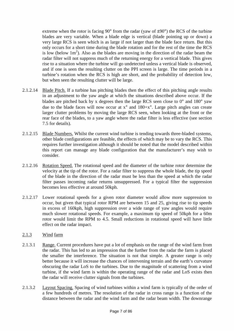
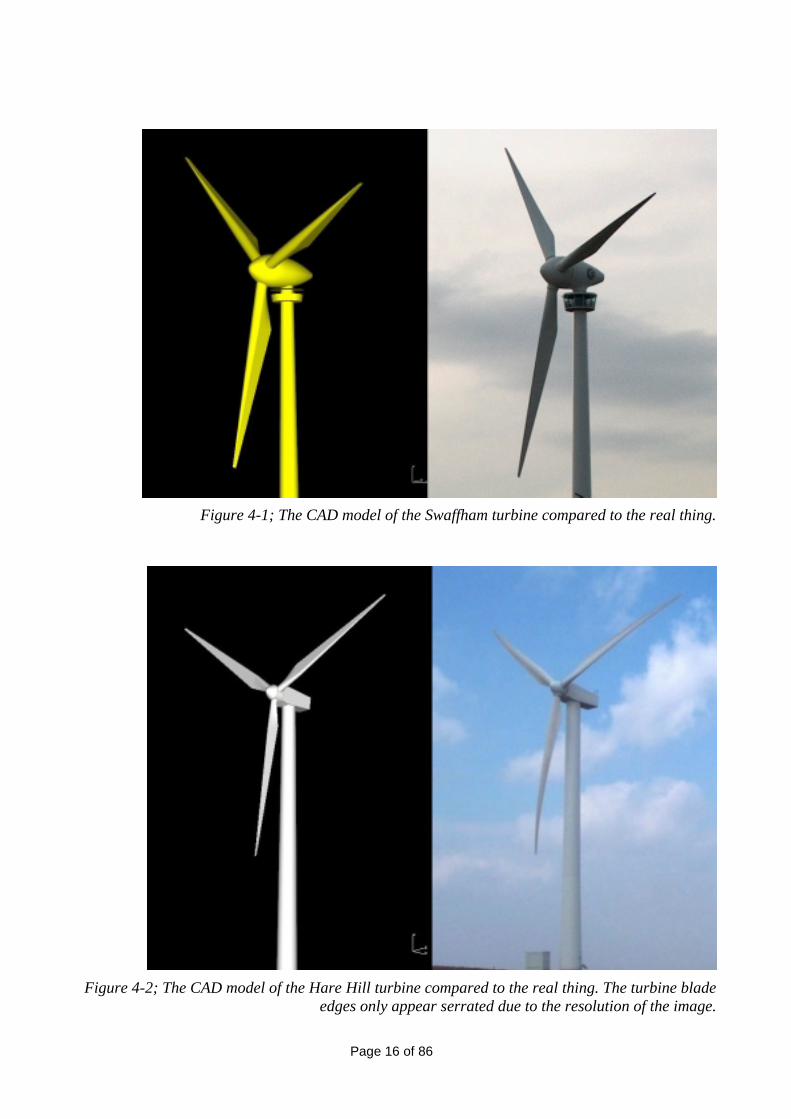
4.3.2 For details of all the approximations made in generating the CAD models see AppendixA.1. Figure 4-1 and Figure 4-2 show the models made as compared to the real turbines.
4.3.3 Four different CAD models were generated as follows:
• Enercon E66 turbine with a 66m diameter rotor;• Vestas V47 turbine with a 47m diameter rotor;• Enercon E66 tower and nacelle with a 80m rotor using NEG Micon blades;• Vestas V47 tower and nacelle with a 52m rotor using NEG Micon blades.
4.3.4 All these CAD models are descriptions of the turbines’ outer surfaces, and no attempt hasbeen made to model the internal structure. The effect of internals on the signature isdiscussed in more detail in appendix A.4.
Page 16 of 86
Figure 4-1; The CAD model of the Swaffham turbine compared to the real thing.
Figure 4-2; The CAD model of the Hare Hill turbine compared to the real thing. The turbine bladeedges only appear serrated due to the resolution of the image.

Page 17 of 86
4.4 Data collected
4.4.1 Far field RCS predictions on all four models described in section 4.3 have been carriedout. Each of the turbines has the same predictions completed on it, carried out in thefollowing way.
4.4.2 For each configuration there are three CAD model descriptions. One has a blade pitch of0° (i.e. the blades are set to catch the maximum wind), one a pitch of 20° (feathered tospill some wind, and 90° (feathered right back to stall the turbine). For each of thesepitches data were collected at 1.5GHz and 3GHz, and at 36 yaw angles of the rotor andnacelle (every 10°). At each of these yaw angles data from 2400 positions of the bladeswere collected to allow simulation of the blade movements in any of the yaw positions.This means over 2 million RCS calculations have been completed. Table 4-1 summarisesthe turbine set-ups predicted.
No of blade pitches 3 {0°, 20°, and 90°}
No. of frequencies 2 3GHz, 1.5GHz
No. of yaw angles 36 0° to 360° in 10° steps
No. of rotor positions foreach yaw
2400 (every 0.05° of rotation)
Table 4-1; Summary of the turbine set-ups predicted on all four turbine configurations.
4.5 Results and analysis
4.5.1 All of the turbine predictions exhibited several basic characteristics. To explain thesecharacteristics the examples of the Enercon turbine at Swaffham (with a blade pitch of 0degrees, at yaw angles of 0 degrees and 90) degrees is used. The RPM for both of thesewere set to 12.4 RPM. A more complete set of the predictions from all the turbines canbe found in Appendix A.5.
4.5.2 In all cases the yaw angle is specified relative to the direction of the radar. So when theyaw is 0° the radar is pointing along the axis of rotation of the turbine rotor, with theblades in front of the tower when viewed from the radar position. This means the turbineis face on to the radar. When the yaw is 90° the turbine rotation axis is perpendicular tothe direction of the radar, i.e. the turbine appears side on to the radar.
4.5.3 We will, firstly, consider the results for the Swaffham turbine at 0 degrees yaw beforeexamining the results for the Swaffham turbine at 90 degrees yaw.
4.5.4 The RCS at 0 degrees yaw is presented in Figure 4-3. It shows a number of features(labelled 1 to 8 on the figure) that can be attributed to the turbine blades. Since we areinvestigating the RCS with time, from a single yaw angle, any contribution to the RCSfrom the tower will be constant. There are two very broad peaks. At the top of which,either side of the maxima, are two further peaks. The symmetry between these isapparent and the likely cause of the observed peaks is the turbine blades. The positions intime of these features are summarised in Table 4-2.

Page 18 of 86
Number Time (secs) Degrees rotated Description
0 0.000 0.0 Initial blade positions (notmarked)
1 ~0.125 ~9.3 Small peak
2 ~0.850 ~63.2 Large peak
3 ~0.980 ~72.9 Small peak
4 ~1.125 ~83.7 Large peak
5 ~1.750 ~130.2 Small peak
6 ~2.450 ~182.3 Large peak
7 ~2.600 ~193.4 Small peak
8 ~2.740 ~203.9 Large peak
Table 4-2; Summary of the main features of the RCS from the Swaffham turbine at 0° yaw
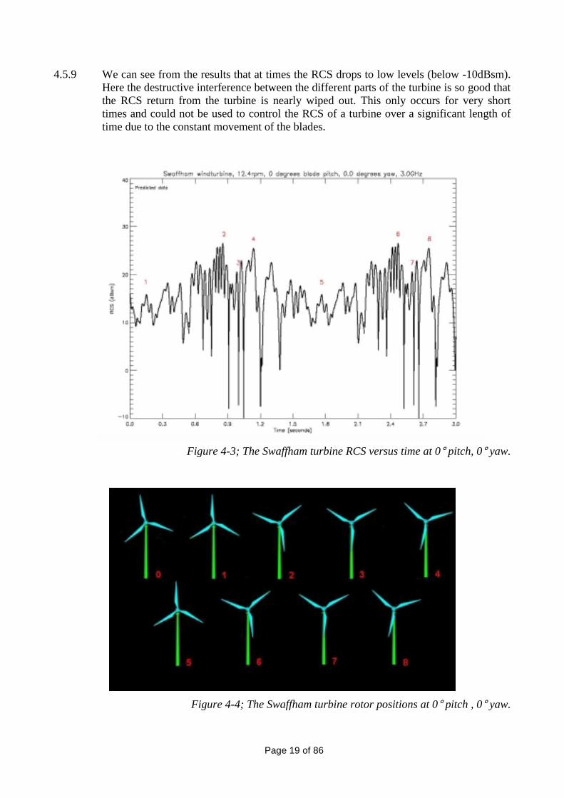
4.5.5 Figure 4-4 details the blade positions at the times indicated in the table above. Position 0is the turbine configuration at time, t = 0. It can be seen that the blade position for thepeaks 2 and 6, and, 4 and 8 are the same respectively. Likewise the small peaks observedat 1 and 5, and, 3 and 7 are also the same. The angular spread between all of these is~120 degrees. This confirms that these small and large peaks are a result of someinteraction with the blades.
4.5.6 We can explain the features observed by considering what is happening to the blades asthey rotate. It may be noted from Figure 4-4 that the peaks (features 2,4,6 and 8 in Figure4-3), occur when a blade is just either side of the tower.
4.5.7 As the blades move the returns from the blades combine with the constant returns fromthe tower and nacelle in different ways. As the returning signals are electromagneticwaves they have a magnitude and a phase (i.e. are phasor quantities). Hence, due toconstructive (in-phase) and destructive (out-of-phase) interference between the differentparts of the turbine, peaks and troughs arise in the RCS pattern.
4.5.8 Furthermore, the inclinations of the blades' surfaces are always changing due to thechanging pitch and rotation of the blades with time. This has the effect of altering theprojected area seen by the radar. The RCS of the blades is closely related to the surfacearea presented to the radar. This, coupled with the interference phenomenon describedabove, will give rise to maxima and minima in a cyclic fashion. The period of thisbehaviour should be equal to the angle between the individual blades, i.e. 120 degrees.
Page 19 of 86
4.5.9 We can see from the results that at times the RCS drops to low levels (below -10dBsm).Here the destructive interference between the different parts of the turbine is so good thatthe RCS return from the turbine is nearly wiped out. This only occurs for very shorttimes and could not be used to control the RCS of a turbine over a significant length oftime due to the constant movement of the blades.
Figure 4-3; The Swaffham turbine RCS versus time at 0° pitch, 0° yaw.
Figure 4-4; The Swaffham turbine rotor positions at 0° pitch , 0° yaw.

Page 20 of 86
4.5.10 This is in fact what is observed in our results. To confirm that the effects seen are fromthe blades, the zero-Doppler (ZD) components were removed from the data. This processremoves all the contributions from the data originating from non-moving parts, i.e. thetower and nacelle. Figure 4-5 presents the data without the ZD components. It can beseen that the same features observed in the complete RCS (Figure 4-3) are present. Thedifference being that the small peaks at points 1 and 5 are approximately 5 dB lower.When the blade positions at these points are considered (see Figure 4-4) we can see thatthe small peaks correspond to when the tower is at its most visible. Therefore the reasonfor the difference in levels is that at this point the RCS is dominated by the returns fromthe tower, which are removed by the ZD processing.
Figure 4-5; The Swaffham turbine RCS versus time at 0° pitch, 0° yaw, with the zero-Dopplercomponent removed.
4.5.11 The RCS at 90 degrees yaw is presented in Figure 4-6. It shows four features (labelled 1to 4 on the figure) that, as with the 0 degrees yaw case, can be attributed to the turbineblades. The figure shows two very sharp spikes in the RCS (labelled 1 and 3) and twoless distinct features between these spikes (labelled 2 and 4). These are summarised inTable 4-3.
4.5.12 The two sharp peaks (1 and 3) can be seen to occur when a blade is pointing verticallydownwards, as shown in Figure 4-7. The radar is looking from right to left in terms of thefigure. When the blade is positioned as shown then the leading edge is both perpendicularand directed towards the radar. The spike is a result of this leading edge. At this point thereturn from the blade will be at its highest.

Page 21 of 86
Number Time (secs) Degrees rotated Description
0 0.000 0.0 Initial blade positions (not marked)
1 ~0.375 ~27.9 Peak
2 ~1.150 ~85.6 Slight Peak
3 ~1.990 ~148.1 Peak
4 ~2.790 ~203.9 Slight Peak
Table 4-3; Summary of the main features of the RCS from the Swaffham turbine at 90° yaw4.5.13 Based on this we might expect to see some sort of event occurring in the RCS when a
blade is pointing directly upwards. This is indeed the case with the very small peaks seenbetween the large spikes (i.e. 2 and 4). Again, the blade positions are shown in Figure4-7. The general flatness of the RCS can be attributed to the fact that the profile of theblades when viewed from 90 degrees yaw is very flat and any subtle effects resultingfrom the blades will be swamped by the return from the tower and nacelle which willdominate.
Figure 4-6; The Swaffham turbine RCS versus time at 0° pitch, 90° yaw
Page 22 of 86
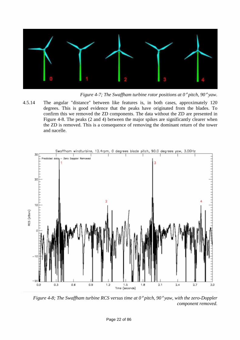
Figure 4-7; The Swaffham turbine rotor positions at 0° pitch, 90° yaw.4.5.14 The angular "distance'' between like features is, in both cases, approximately 120
degrees. This is good evidence that the peaks have originated from the blades. Toconfirm this we removed the ZD components. The data without the ZD are presented inFigure 4-8. The peaks (2 and 4) between the major spikes are significantly clearer whenthe ZD is removed. This is a consequence of removing the dominant return of the towerand nacelle.
Figure 4-8; The Swaffham turbine RCS versus time at 0° pitch, 90° yaw, with the zero-Dopplercomponent removed.

Page 23 of 86
4.6 Summary
4.6.1 We have explained the various features (peaks and troughs) on the predicted RCS for theSwaffham wind turbine at two yaws (0 degrees and 90 degrees). The blades contributeless when viewed from side-on (90 degrees yaw) than at head-on (0 degrees yaw) interms of average RCS. However, in both cases the dominant features, such as the peaksin the RCS, are a direct result of the turbine blades.

Page 24 of 86
This page is intentionally blank
Page 25 of 86
5 RADAR MEASUREMENTS
5.1 Scale model measurements
5.1.1 To add confidence and credibility to the RCS prediction process and the results for thisproject, one of the blade designs supplied by NEG Micon Rotors was made into a 1/15th
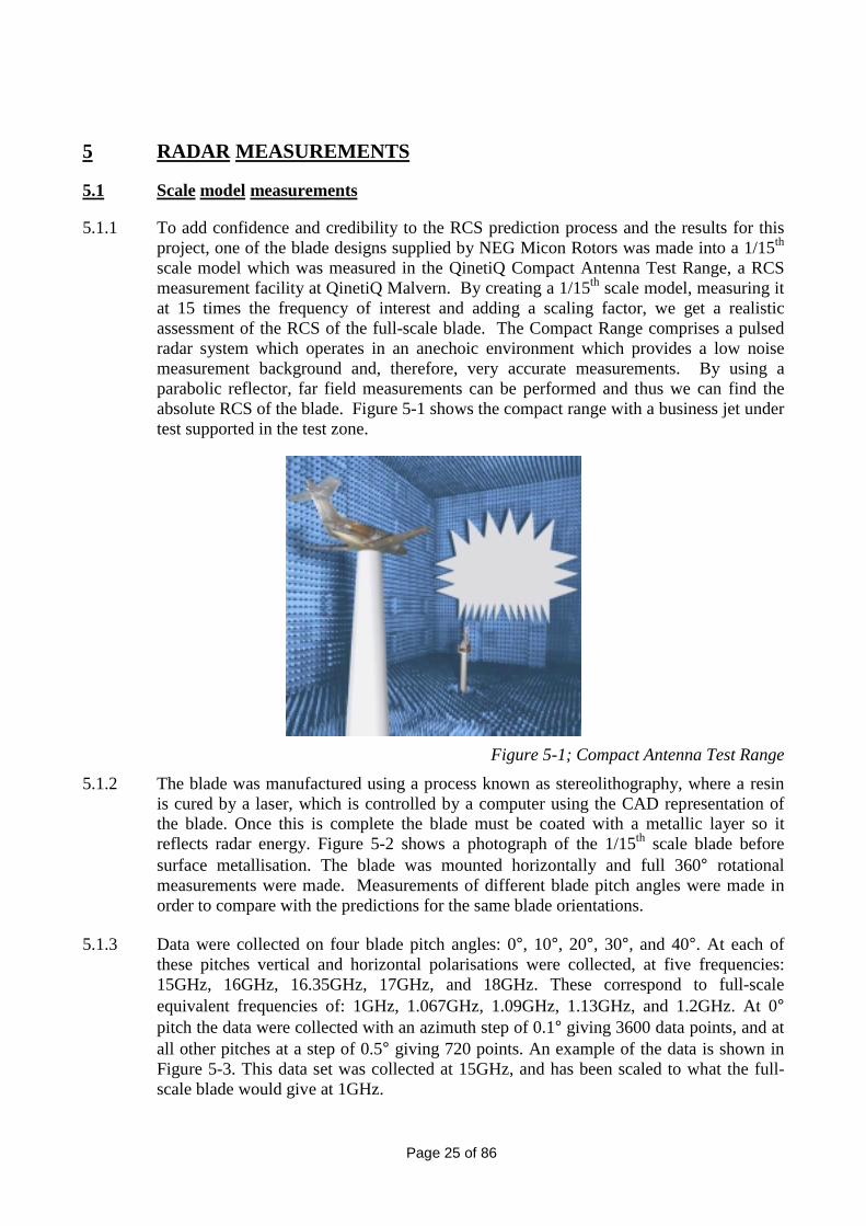
scale model which was measured in the QinetiQ Compact Antenna Test Range, a RCSmeasurement facility at QinetiQ Malvern. By creating a 1/15th scale model, measuring itat 15 times the frequency of interest and adding a scaling factor, we get a realisticassessment of the RCS of the full-scale blade. The Compact Range comprises a pulsedradar system which operates in an anechoic environment which provides a low noisemeasurement background and, therefore, very accurate measurements. By using aparabolic reflector, far field measurements can be performed and thus we can find theabsolute RCS of the blade. Figure 5-1 shows the compact range with a business jet undertest supported in the test zone.
Figure 5-1; Compact Antenna Test Range5.1.2 The blade was manufactured using a process known as stereolithography, where a resin
is cured by a laser, which is controlled by a computer using the CAD representation ofthe blade. Once this is complete the blade must be coated with a metallic layer so itreflects radar energy. Figure 5-2 shows a photograph of the 1/15th scale blade beforesurface metallisation. The blade was mounted horizontally and full 360° rotationalmeasurements were made. Measurements of different blade pitch angles were made inorder to compare with the predictions for the same blade orientations.
5.1.3 Data were collected on four blade pitch angles: 0°, 10°, 20°, 30°, and 40°. At each ofthese pitches vertical and horizontal polarisations were collected, at five frequencies:15GHz, 16GHz, 16.35GHz, 17GHz, and 18GHz. These correspond to full-scaleequivalent frequencies of: 1GHz, 1.067GHz, 1.09GHz, 1.13GHz, and 1.2GHz. At 0°pitch the data were collected with an azimuth step of 0.1° giving 3600 data points, and atall other pitches at a step of 0.5° giving 720 points. An example of the data is shown inFigure 5-3. This data set was collected at 15GHz, and has been scaled to what the full-scale blade would give at 1GHz.

Page 26 of 86
Figure 5-2 Non-metallised 15th scale NEG Micon Rotors blade.
-70
-60
-50
-40
-30
-20
-10
0
10
20
30
-180 -150 -120 -90 -60 -30 0 30 60 90 120 150 180
Angle (degrees)
RCS(dBsm)
Figure 5-3; RCS of blade at full-scale frequency of 1GHz with blade at 0 degree pitch. Polarisationis vertical.
5.1.4 The leading edge of the blade is presented to the radar at 0°. Here the RCS rises to amaximum of 22dBsm. At 90° the tip of the blade is facing the radar, and the RCS is only-14dBsm. At 180° the trailing edge is facing the radar. This is angled slightly soproducing a peak of 14dBsm at -175°. The return at -90° is when the blade root is facingthe radar, which could not occur when attached to a turbine hub.
Page 27 of 86
5.2 RCS prediction validation with a scale model blade
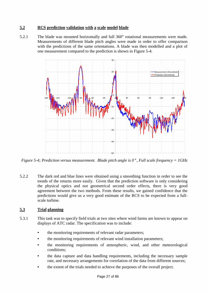
5.2.1 The blade was mounted horizontally and full 360° rotational measurements were made.Measurements of different blade pitch angles were made in order to offer comparisonwith the predictions of the same orientations. A blade was then modelled and a plot ofone measurement compared to the prediction is shown in Figure 5-4.
-50
-40
-30
-20
-10
0
10
20
30
-180 -150 -120 -90 -60 -30 0 30 60 90 120 150 180
MeasurementPredictionMeasurement (Smoothed)Prediction (Smoothed)
Figure 5-4; Prediction versus measurement. Blade pitch angle is 0° , Full scale frequency = 1GHz
5.2.2 The dark red and blue lines were obtained using a smoothing function in order to see thetrends of the returns more easily. Given that the prediction software is only consideringthe physical optics and not geometrical second order effects, there is very goodagreement between the two methods. From these results, we gained confidence that thepredictions would give us a very good estimate of the RCS to be expected from a full-scale turbine.
5.3 Trial planning
5.3.1 This task was to specify field trials at two sites where wind farms are known to appear ondisplays of ATC radar. The specification was to include:
• the monitoring requirements of relevant radar parameters;• the monitoring requirements of relevant wind installation parameters;• the monitoring requirements of atmospheric, wind, and other meteorological
conditions;• the data capture and data handling requirements, including the necessary sample
rate, and necessary arrangements for correlation of the data from different sources;• the extent of the trials needed to achieve the purposes of the overall project.

Page 28 of 86
This specification was to be sufficient for any third party to conduct the trials and wouldsupply all the data needed to successfully validate the computer model. The outline trialsplan generated from this task can be found in appendix C.
5.3.2 QinetiQ required full-scale radar measurements of wind turbines to provide radar data forvalidation of the computer model (WHIRL). The plan was to use an instrumentationradar to make radar measurements of a single wind turbine at Swaffham, Norfolk, and torecord the information from the Watchman radar sited at Marham Royal Air Force (RAF)base. Also data would be recorded from the primary radar at Prestwick of the twenty-turbine wind farm at Hare Hill, Ayrshire, Scotland. Each site has particularcharacteristics: the Swaffham site is located about 5nmi from an ATC radar at the RAFairfield at Marham, and, being a single turbine, will form a good experimental ‘control’,and the Hare Hill site is well-known for the clutter it causes on the ATC PPI radardisplays at Prestwick Airport. No instrumentation radar measurements were to take placeat Prestwick.
5.3.3 In order to collect the data from the primary radar at Marham and Prestwick QinetiQsought a contractor who would be able to offer this service. Contact with RAF StrikeCommand informed QinetiQ that Flight Refuelling Ltd (FRL) was the manufacturer ofthe RAF’s current ATC displays for their Watchman primary airfield radar and also thatthe company had a display recording system that is used by FRL as a service tool. A visitwas made by QinetiQ to FRL to discuss requirements, and to see a demonstration of PPIrecording playback. FRL immediately understood the requirement and the demonstrationshowed that the PPI playback matched our need. The result was that FRL would be sub-contracted for these aspects of the trials.
5.3.4 Exploration of QinetiQ instrumentation radar resources showed that our MultibandPulsed Radar (MPR), could match the needs of the trials programme. MPR, althoughclassed as a mobile radar, is built into four shipping containers that are permanentlyattached to two 40 ft-long articulated trailers. MPR presently operates on the 3 GHzfrequency of ATC primary radar systems.
5.3.5 Along with collecting the radar data the MPR also logs the current weather conditions,against time so that this information can be linked to the measurement. It also collectsvideo footage of the wind turbine when it collects radar data, so that visual checks of thecurrent state of the turbine can be made.
5.3.6 Another important part of the trial is the collection of data from the turbine. This must belogged against time so that the radar measurements and the turbine data can be linkedtogether. We planned to collect the data direct from the turbines’ control systems using aPC.
5.4 Swaffham trial
5.4.1 The Swaffham trial took place from 1 July 2002 to 5 July 2002, and was successfullycompleted.
5.4.2 The QinetiQ MPR was stationed at Swaffham Raceway, 3.45km from the Ecotricitywind turbine (see Figure 5-5). Radar observations of the turbine were made at regularintervals over a period of five days, during which a variety of weather conditions wereexperienced. Views of the turbine varied by more than 180° in yaw angle, with more than

Page 29 of 86
half of the aspects being seen during both wet and dry conditions (see Figure 5-6). Intotal, nearly 250 RCS measurements of the turbine were recorded, lasting between oneand two minutes each. These data are split roughly half-and-half between linearhorizontal and linear vertical polarisations, and can be calibrated for absolute RCS usingsphere measurements made at the site.
Figure 5-5; The MPR radar on site at Swaffham, with the wind turbine visible in the distance.

Page 30 of 86
North
MPR
Wet weather measurements
Dry weather measurements
Figure 5-6: Rough sketch showing turbine heading during measurements. Dotted lines for drymeasurements, shaded areas for wet-weather measurements
5.4.3 Output from the radar at RAF Marham was also successfully collected by FRL. This waslater analysed at QinetiQ using kit supplied by FRL.
5.4.4 The data from the turbine control system were also collected without problems, largelythanks to the help and assistance of Ecotricity, the turbine operators. They supplied a PCthat was hooked up to the turbine supervisory control and data acquisition (SCADA)system to record all the turbine settings every 3 seconds for the duration of the trial. Datacollected from the turbine were rotor revolutions per minute (RPM), pitch of each blade,and yaw angle of the turbine. What this data set lacked was a means to identify where theblades were in their rotation cycle at any given time. To do this QinetiQ developed asensor (see appendix D.4 for details) to record this from within the nacelle. This workedwell in lab testing, but in the nacelle of the turbines it suffered problems fromelectromagnetic interference and vibration. Data lost due to these problems wereinterpolated and correlated to the turbine blade positions from the recorded RCS data,and from the MPR video footage.
5.5 Swaffham results
5.5.1 To give an example of the results collected from the MPR trial, a typical data set isexamined. All the main scattering features of the turbine are identified. More results arecontained in Appendix D.5.

Page 31 of 86
5.5.2 To give a sense of scale to these results Figure 5-7 shows a range of RCS values andwhere different objects lie on this scale. This shows why wind turbines are easilydetected by radar as their scattering magnitude puts then up with some of the largestaircraft targets. Any operating ATC radar must be sensitive enough to see the smallaircraft, which tend to have RCS of about 1m2 to 10m2, where as the turbine return is upto 1000m2 in some instances.
Typical RCS values (from textbook)
-40 -30 -20 403020100-10
0.0001 0.001 0.01 0.1 1.0 10 100 1000 10000m²
dBsmInsects Birds Man
SmallAircraft
Jumbojet
Ships
Windturbines
Figure 5-7; RCS scale showing the relative scattering magnitudes of different objects.
5.5.3 A set of data was identified during which the turbine was rotating at almost constantmaximum speed (23 RPM). Using the video footage recorded by the radar, times werededuced for the start and end of three full rotations, so that RCS data could be extractedfor just this period (16:25:00.02 to 16:25:08.00, 1/7/2002). The calibrated RCS andspectra for the first revolution are shown in Figure 5-8 and Figure 5-9. Doppler spectrafor the whole period are shown in Figure 5-10.
0 0.1 0.2 0.3 0.4 0.5 0.6 0.7 0.8 0.9 1 1.1 1.2 1.3 1.4 1.5 1.6 1.7 1.8 1.9 2 2.1 2.2 2.3 2.4 2.5 2.6 2.7 2.8 2.9 30
5
10
15
20
25
30
35
Time (s)
RCS
(dB)
RCS from SWT008
Figure 5-8; Calibrated RCS for (just over) one full revolution

Page 32 of 86
5.5.4 Frame-by-frame analysis of the video allowed approximate timings to be deduced for theoccasions when a blade was either vertical or horizontal with respect to the radar line ofsight. These blade positions correspond to expected maxima and minima of the RCS fora single blade, and hence might be expected to give rise to peaks and troughs in theoverall turbine RCS pattern. The times for these events are listed in Figure 5-11.Comparison with the peak positions in the RCS plot, Figure 5-8, shows a fair correlationbetween the video timings and the locations of peak RCS levels.
5.5.5 Considering Figure 5-8, it can be seen that there are three repetitions of approximatelythe same RCS variation during a single revolution, giving nine RCS peaks. Since thereare three turbine blades, spaced at 120°, we expect to see 6 'flashes' as each blade passesthrough the vertical, above and below the hub. It is proposed that the three additionalRCS peaks correspond to dihedral scattering, occurring half-way between the verticalflashes as incident radar energy is reflected from one blade onto the other beforereturning to the receiver. This scattering may be at a maximum when the blade furthestfrom the radar is horizontal, so that the radar is looking along the axis of the dihedralformed by the other two blades.
Time (s)
Dop
pler
(Hz)
Spectra from SWT008
0 0.1 0.2 0.3 0.4 0.5 0.6 0.7 0.8 0.9 1 1.1 1.2 1.3 1.4 1.5 1.6 1.7 1.8 1.9 2 2.1 2.2 2.3 2.4 2.5 2.6 2.7 2.8 2.9 3
-1500
-1000
-500
0
500
1000
1500
Figure 5-9; Doppler spectra versus time corresponding to the RCS plot

Page 33 of 86
-80
-60
-40
-20
0
20
Time (s)
Dop
pler
(Hz)
0 1 2 3 4 5 6 7 8
-1000
-500
0
500
1000
1500
Figure 5-10; Spectrum against time for three full revolutions
2.72
2.30 2.522.061.82
0.52 0.740.280.00
1.40 1.641.160.94
Figure 5-11; Approximate timings of blade positions (in seconds), taken from video
dB

Page 34 of 86
5.5.6 So at this point the blades are in the position shown in Figure 5-11, at 0.52 seconds, withthe radar looking from the left of the page and the rotor turning clockwise. We willdefine blade 1 as the horizontal blade, blade 2 as the lower blade and blade 3 as the upperblade. As the blades continue to rotate blade 3 will approach vertical, where the bladetip’s velocity vector is pointing directly away from the radar, hence negative Dopplerfrequencies are observed. The Doppler frequency generated by blade 2 is decreasing asthe blade approaches horizontal, and is overtaken by the Doppler contribution from theapproaching blade 1. When blade 1 reaches vertical (1.16 seconds in Figure 5-11), we geta maximum positive value in the Doppler frequency as now blade 3 has a velocity vectorpointing directly towards the radar.
5.5.7 The spectrum from the vertical blade has a curved maximum region (dark red in thefigures), which starts just before the blade reaches vertical and rapidly moves towardszero Doppler. This can be interpreted as a strong return moving from the blade tip downtowards the root of the blade, and could be from the front or back edge, depending on theblade curvature.
5.6 Wind farm trial
5.6.1 A trial using the wind farm known as Hare Hill in Scotland was due to be completed tocollect data from a wind farm with several wind turbines in site of a radar at Prestwickairport. Unfortunately the data available from the turbines was not suitable for the trialand budgetary constraints meant adding instrumentation to provide this data was notpossible.
5.6.2 However some video of the PPI display at Prestwick was collected and this has been usedfor validation in section 6.5.5.

Page 35 of 86
6 VALIDATION OF THE COMPUTER MODEL
6.1 Validation philosophy
6.1.1 To validate the WHIRL-COM model using the data collected at Marham, we havebroken the process down in to three separate areas for which we wish to makecomparisons against the real measurement data. This comes from the requirement tovalidate not only WHIRL but also the two data libraries it requires. This means weneeded to validate not just against the output of WHIRL but also the input libraries thatthe code runs from. These two libraries contain the RCS data for the turbines used in thesimulation and the propagation data for the particular radar in question. Both of theselibraries were validated using the output from the MPR data collected at Marham. Oncethese libraries were shown to be correct we then validated the WHIRL software with thePPI data collected from the Watchman at RAF Marham.
6.1.2 The prediction data were collected sometime before the trial took place and hence aperfect match in the set up of the measured and the predicted scenarios was not possible.Nevertheless, the differences are small and should not greatly influence the results.
6.2 RCS validation
6.2.1 Overview
6.2.1.1 In order to validate the RCS predictions it was necessary to compare them withmeasurement data taken from equivalent turbine configurations.
6.2.1.2 We have measurement data from the Swaffham trial for a number of different scenarios(see section 5.4). The measurement configurations used in our comparison aresummarised in Table 6-1.
Data set Yaw (degs) Pitch (degs) AverageRPM
Frequency(GHz)
1 0.4 0.96 12.4 3.05
2 100.33 0.99 12.5 3.05
3 39 0.99 20.6 3.05
4 0 0 10.7 3.05
5 50 5 22.5 3.05
6 100 0 13.6 3.05
Table 6-1; Summary of the measurement configurations used in the RCS validation

Page 36 of 86
6.2.1.3 It should be noted that the turbine orientation of our prediction data does not exactlymatch those of the measurements. A comparison of the predicted orientations and themeasured are summarised in Table 6-2. The differences are all very small and likelydifferences in the RCS will be small enough to allow effective comparisons. Also themeasurement data refer to average or estimated values of yaw, blade pitch and RPM. Wewill be referring to the orientation of our modelled turbine throughout the followingsubsection.
Measured Predicted
Yaw (degs) Blade Pitch (degs) RPM Yaw(degs)
Blade Pitch (degs) RPM
0.4 0.96 12.4 0 0 12.4
100.33 0.99 12.5 100 0 12.5
39 0.99 20.6 40 0 20.6
0 0 10.7 0 0 10.7
50 5 22.5 50 5 22.5
100 0 13.6 100 0 13.6
Table 6-2, Summary of the measured and predicted turbine orientations
6.2.2 Swaffham turbine at 0 degrees yaw, 0 degrees pitch
6.2.2.1 The results of the comparison between the measurement and predicted RCS data for theturbine viewed from `head-on' (0 degrees yaw) are presented in Figure 6-1. It can be seenin this figure that the two sets of data match very closely in terms of a general trend andlevel. The main differences are a number of peaks that are not fully reproduced by thepredictions. This is due to two effects; 1) the reflectivity of the blades and 2) a scatteringphenomenon known as “multiple bounce” returns. The reflectivity of our blades was anestimate based on the reflectivity of fibreglass, but it appears the blades are morereflective than expected hence, the predictive values are lower than the measured values.The scattering due to multiple bounce returns was not computed as part of the predictionsdue to the computational overhead involved. Where paths exist back to the radar via twoor three bounces from the turbine structure the predictions will be lower than themeasurements. This is discussed more fully in the conclusions to this section.

Page 37 of 86
Figure 6-1; Comparison of the measured and predicted Swaffham turbine RCS versus time at 0°pitch, 0° yaw, 12.4RPM.
6.2.3 Swaffham turbine at 100 degrees yaw, 0 degrees pitch
6.2.3.1 At 100 degrees yaw we find that the measured and predicted RCS values are very close.The comparisons between the two data sets are presented in Figure 6-2. Here the meanRCS levels are within 2 to 3dB of each other and a very good match has beendemonstrated. This indicates that the multiple bounce paths back to the radar are notsignificant at this yaw angle.

Page 38 of 86
Figure 6-2; Comparison of the measured and predicted Swaffham turbine RCS versus time at 0°pitch, 100° yaw, 12.4RPM.
6.2.4 Swaffham turbine at 50 degrees yaw, 0 degrees pitch
6.2.4.1 In Figure 6-3 the comparison between the measured and predicted data is presented forthe turbine at 50 degrees yaw. Overall the agreement is good with all the main featuresreplicated by the predictions.
6.2.4.2 Away from the blade flashes the prediction data are higher than the measurements byaround 5dB, and as with the 0° yaw data the peaks in the predictions are down on themeasurement equivalent by around 4dB. These differences can be accounted for, aspreviously, by a lack of multiple bounce data in the predictions and differences in theblade reflectivity. The reason for the predictions being 5dB higher than the measurementsaway from the peaks is to do with the model of the nacelle used. In the predictions thenacelle is a perfectly smooth object and so produces a strong specula return at yaw anglesnear 40 to 50°. This effect in the measurements is smaller because the nacelle curvatureis not as consistent and this causes the scattering to be incoherent. These differences arenot critical in the modelling of the turbine response and the level of accuracy issufficient.
Page 39 of 86
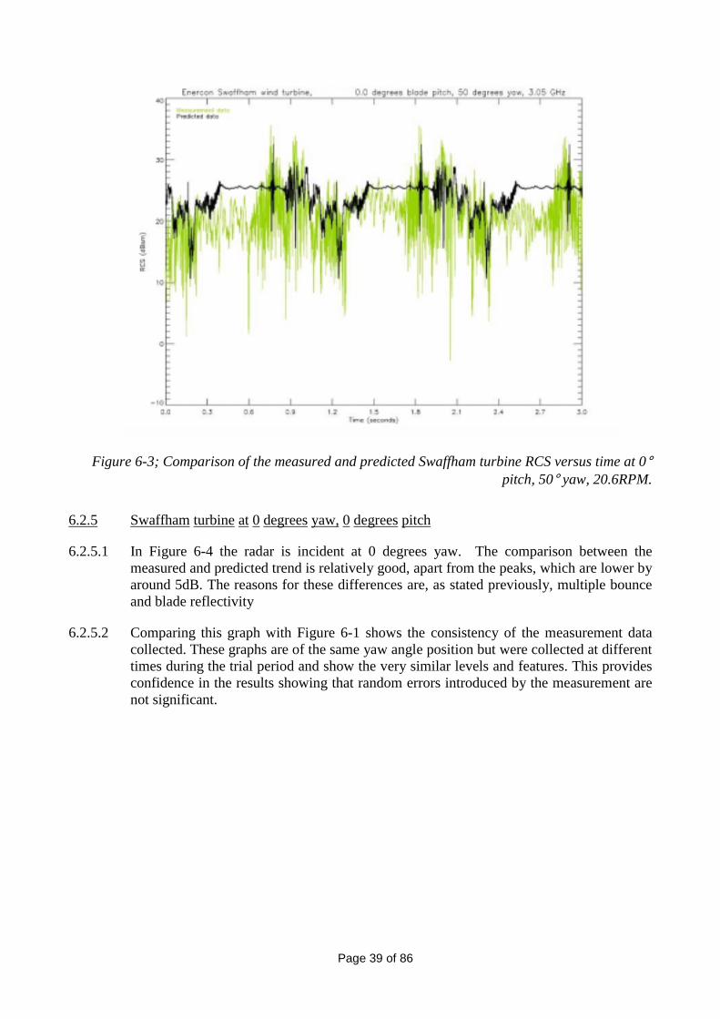
Figure 6-3; Comparison of the measured and predicted Swaffham turbine RCS versus time at 0°pitch, 50° yaw, 20.6RPM.
6.2.5 Swaffham turbine at 0 degrees yaw, 0 degrees pitch
6.2.5.1 In Figure 6-4 the radar is incident at 0 degrees yaw. The comparison between themeasured and predicted trend is relatively good, apart from the peaks, which are lower byaround 5dB. The reasons for these differences are, as stated previously, multiple bounceand blade reflectivity
6.2.5.2 Comparing this graph with Figure 6-1 shows the consistency of the measurement datacollected. These graphs are of the same yaw angle position but were collected at differenttimes during the trial period and show the very similar levels and features. This providesconfidence in the results showing that random errors introduced by the measurement arenot significant.

Page 40 of 86
Figure 6-4; Enercon turbine at Swaffham, 0 degs pitch, 0 degs yaw, 10.7RPM.
6.2.6 Swaffham turbine at 50 degrees yaw, 5 degrees pitch
6.2.6.1 In Figure 6-5 we can see the prediction data compared with the measurement data for theturbine when the blade has been pitched at ~5 degrees. It can be observed that there is areasonable level of agreement between the two data sets. The predictions are generallyhigher than the measurements, bar one repeating peak that is not found in the predicteddata. The higher prediction levels are due to a strong return from the nacelle that is notpresent in the measurement due to imperfections in the nacelle which are not modelled inthe predictions.
6.2.7 Swaffham turbine at 100 degrees yaw, 0 degrees pitch
6.2.7.1 There is exceptionally good agreement at 100 degrees yaw (see Figure 6-6) between thepredicted and measured data in terms of trend and magnitude. The predicted data arelower than the trial data by around 2dB.

Page 41 of 86
Figure 6-5; Enercon turbine at Swaffham, 5 degs pitch, 50 degs yaw, 22.5RPM
Figure 6-6; Enercon turbine at Swaffham, 0 degs pitch, 100 degs yaw, 13.6RPM

Page 42 of 86
6.2.8 Conclusions
6.2.8.1 The RCS predictions of the Swaffham turbine discussed in the previous sub-section havebeen compared to measurement data successfully. The positions of the peaks and basictrend of the measurement data were shown to be accurately predicted. The level ofagreement is sufficient for the current purpose and the differences are understood andexplainable.
6.2.8.2 It was noted that some of the predictions are 4 to 6 dB lower than the measurements, nearRCS peaks. EMRAD noted this in their review of the model – see appendix G. Onfurther consideration it was concluded that this is the result of two main factors.
6.2.8.3 Firstly, the blades are modelled as solid fibreglass bodies. The properties of the fibreglasswe used give rise to an 8dB reduction in the returns emanating from the blades. Theblades appear to be more reflective increasing the level of the measurement data over thepredictions.
6.2.8.4 Secondly, the predictions carried out do not model any returns resulting from multipleinteractions within the turbine structure. An example of this would be energy reflected bya blade onto the tower and then returned to the radar. This effect is commonly referred toas “multiple-bounce” returns. The Ocellus prediction code is capable of predictingmultiple bounce returns from a structure, but this has not been computed because of thecomputational overhead involved if calculated for a full rotation of the blades. Givengeometry that gives rise to paths back to the radar via multiple bounce these returns canbe very large. Without this mechanism the predictions will be different from themeasurement where strong multiple bounce returns are present.
6.2.8.5 To overcome this difference we must deal with both of these factors. The turbine bladesneed to be modelled with a more realistic reflectivity. It should be noted that the genuineblades are fibreglass shells, containing lightning conductors and have metal tips. Theshell structure and metallic elements will undoubtedly affect the level of the RCS.Reflectivity values would ideally come from small scale measurements of the materialsinvolved, but if this was not possible then a more reflective blade could be modelled tomake sure the predictions do not fall below the actual scattering levels.
6.2.8.6 The multiple bounce calculations must be included in the turbine calculations. To predictthis mechanism for the complete detailed model is not impossible but is a timeconsuming process. A better solution might be to calculate the multiple bounce on asimplified turbine and then add these results into the final solution. Some investigationwould need to be carried out to find the right trade-off between accuracy andcomputational efficiency, so that the predictions could be carried out in an optimum way.
6.2.8.7 At around 40 to 50° yaw the predictions showed a higher RCS than the measurements attimes when the blades are not causing large returns. At these points the RCS isdominated by the scattering from the nacelle, which in the computer model of the turbinegives a stronger return than observed from the measurements. This is due to the modelnacelle being a perfectly smooth object creating a large specula return at this yaw angle.This is not seen in the measurements due to imperfections in the nacelle surface.

Page 43 of 86
6.3 Spectral content validation
6.3.1 To further validate the predictions we have looked at the spectral content of the returningsignal as compared to the measured data. To make the comparison the measurement dataand prediction data were processed using the same Fourier transform routine. Themeasurement data were re-sampled at the rate of the collected prediction data to allow acomparison to be made.
6.3.2 The spectra have been calculated using a complete revolution of the rotor, so shows thefrequency content averaged over the whole cycle. We expect to see negative and positivefrequency components for parts of the cycle when a blade is moving towards and awayfrom the radar. The maximum significant frequency component should match up to theblade tip speed in the direction of the radar.
6.3.3 Yaw -100° and an RPM of 16.5 comparison
6.3.3.1 Figure 6-7 shows the results of this comparison. The main features to note are the largezero Doppler spike showing a large part of the turbine has no movement relative to theradar (tower and nacelle). This is present in both the prediction and the measurement andthey are within 1dB of each other in magnitude.
6.3.3.2 The prediction data show a sharp cut-off at around ±1170Hz. This corresponds to a bladetip speed of 58.5ms-1. Calculating the tip speed from the rotation rate of 16.5 RPM givesa tip speed of 57ms-1, a good match. Beyond this frequency there are no data and we areleft with the noise level. For the measurements this is around 50dB and in thepredictions, a much cleaner data-set, this is down at –80dB. These differences are notimportant when studying these graphs.
6.3.3.3 The effect of the higher noise level on the measurement data is that the highest frequencycomponent is not as distinct due to the higher noise level. Also the real turbine has moredegrees of freedom. Vibration, sway and flex will all give rise to spectral componentsthat are not modelled in the prediction.
6.3.3.4 Overall the measurements and the predictions show a good level of agreement withsimilar patterns and the same basic features.

Page 44 of 86
Figure 6-7; Frequency spectrum for one revolution of the Enercon E-66 turbine, measured andpredicted comparison. Yaw -100°, Pitch 0°, RPM 16.5.
6.3.4 Yaw 10° and RPM of 12.4 comparison
6.3.4.1 Figure 6-8 shows the comparison when looking at 10° yaw. This is close to lookingnormal to the rotor when the spectral content will be smaller as the blades do not movemuch in the direction of the radar.
6.3.4.2 As before both the data-sets show a zero Doppler spike and then frequency componentsup to the blade tip speed in the direction of the radar. The slower drop-off in spectracomponents seen in the measurement data is probably due to the greater range ofmovement possible for the real turbine. The prediction roll-off frequency is ±160Hzwhich corresponds to a tip speed of 8ms-1 in the direction of the radar. Working from theRPM and the yaw angle we get a tip speed of 7.8ms-1 in the radar direction, a good match.
6.3.4.3 Results agree well out to the tip speed frequency of ±160Hz, then beyond this frequencythere is some extra frequency components in the measurement data from movement notmodelled in the predictions (i.e. flex and bending of the blades and tower). Data –50dBor lower are not significant as this is the noise floor of the measurements.
6.3.5 Yaw 90° and 12.5 RPM comparison
6.3.5.1 Figure 6-9 shows the comparison with a yaw of 90°. Again the main features to note arethe large zero Doppler return shown in both data sets and the cut-off frequency thatoccurs at ±850Hz. This corresponds to a tip speed of 42ms-1. Using the RPM we find atip speed of 43ms-1, a good match.

Page 45 of 86
6.3.5.2 The comparison shows the main features are replicated, with the predictions being at aslightly lower level than the measurements.
Figure 6-8; Frequency spectrum for one revolution of the Enercon E-66 turbine, measured andpredicted comparison. Yaw -10°, Pitch 0°, RPM 12.4
Figure 6-9; Frequency spectrum for one revolution of the Enercon E-66 turbine, measured andpredicted comparison. Yaw 90°, Pitch 0°, RPM 12.5
Page 46 of 86
6.4 Propagation validation
6.4.1 The validation of the propagation model has been limited to a simple comparisonbetween NEMESIS (used for input to WHIRL) predictions and those from anotherwidely used model, the Advanced Refractive Effects Prediction System (AREPS version2.01.2014). This is produced by the Space and Naval Warfare Systems Center, SanDiego, Atmospheric Propagation Branch.
6.4.2 The scenario chosen for comparison was a simulation of the MPR looking at theSwaffham wind turbine. The radar was placed at 52°39.2'N, 0°37.9'E, at a height of 2mabove ground level. The direction of illumination was 085°, at 2° elevation, using afrequency of 3.05GHz. A vertical slice prediction was made with both models, showingthe one-way path loss as a function of height and range. Results are shown in Figure 6-10and Figure 6-11, which have been plotted using the same scales as far as possible. Thegraphs show the one-way path-loss for a bearing from the radar, taking into account theterrain. The terrain is a brown colour in both of the plots at the bottom of each graph, andthe other colours show the path-loss at a range and height from the radar. The AREPSplot only shows data below an elevation angle from the radar of 45°, hence the area of nocolour in the top left of the plot. We can see areas of high loss close to the ground wherethe terrain is screening the radar’s view and a lobe structure as the elevation angle isincreased. These lobes are caused by energy travelling via the ground and energytravelling directly from the radar constructively interfering with each other to create alobing pattern. The NEMESIS output has more subtle variations in colour, makingcomparison difficult, but it shows broadly similar features to the AREPS output.
6.4.3 This is only a one-off comparison, but other projects within QinetiQ have used theNEMESIS propagation model successfully. One such project states that the model hasbeen tested and accepted for maritime radar studies at 3GHz. This project confirmed thatNEMESIS predictions of propagation factor, as a function of height and range, wereconsistent with measurements for the VHF band. Comparisons in the general literatureindicate that NEMESIS agrees well with ray optics and diffraction solutions in theirrespective regions of validity, and that NEMESIS agrees with other parabolic waveequation solutions.

Page 47 of 86
-180
-170
-160
-150
-140
-130
-120
-110
-100
-90
Range (km)
Hei
ght (
m)
1 2 3 4 5 6 7 8 9 100
20
40
60
80
100
120
140
160
180
200
Figure 6-10; 1-way path loss from NEMESIS
Figure 6-11; AREPS propagation loss prediction

Page 48 of 86
6.5 WHIRL validation
6.5.1 Scenarios tested
6.5.1.1 To carry out the validation a few scenarios were picked so that the turbine returns couldbe studied and compared with the results from WHIRL. The comparison is done based onthe physical size of the turbine return, and the number of times in 50 radar scans theturbine is "hit" or "missed" by the radar. We maintained a consistent approach whencomparing the predictions with the real display. Table 6-3 lists the scenarios investigated.
6.5.1.2 As an example of the radar picture at Marham an image with a range of 13nmi is shownin Figure 6-12. Here the wind turbine can be seen as a small yellow return, along withother clutter that appears to be from trees, road traffic and other large man-madestructures, plus several aircraft targets. To examine the clutter caused by the turbine wehave zoomed right in on its position to get the best view. This is clearly not how the radaroperators would use the PPI but is required to properly compare the simulation with thereal data.
Date Time Turbine RPM Turbine bladePitch
Turbine Yawangle (fromradardirection)
02/07/2002 17:26 23 6 39
04/07/2002 16:06 12.4 1 0.4
05/07/2002 12:20 12.5 1 93
01/07/02 18:18 Turbine switchedoff
90 28
Table 6-3; Turbine configurations investigated for validating WHIRL

Page 49 of 86
Figure 6-12; Screen shot from the recorded Marham data showing the turbine return and some airtraffic.
6.5.2 Turbine at 40° yaw
6.5.2.1 The first scenario tested has the turbine at 40° yaw to the radar with a pitch of 6° and arotation speed of 23 RPM. Referring to the RCS data from the turbine in Figure 5-8 andFigure 6-3, when not close to either 90° yaw or 0° yaw from the radar direction, thesignature levels of the turbine have similar characteristics. The major differences in thescattered energy occur in the frequency spectrum.
6.5.2.2 To compare the data from WHIRL with the recorded picture, two parameters wereconsidered; the size of the return on the screen and the amount of valid hits seen in asample of 50 radar revolutions. Examples of a valid hit and a miss are shown for thesimulation and the recorded data in Figure 6-13 and Figure 6-14. The radar display showshits in the last scan as yellow and then this fades with each subsequent scan of the radarwithout a hit to orange though to black. The colours and persistence of the plots can beset by the user of the display. In WHIRL we have only modelled the clutter caused by theturbine, which is shown in Figure 6-13 and Figure 6-14 as the central orange or yellowplot. The other plots seen in the real radar display are from other clutter sources notassociated with the wind turbine.
6.5.2.3 The size of the return from the wind farm when a good hit is returned in the real data is410m in azimuth and 160m in down range. In the prediction large returns are 400m in

Page 50 of 86
azimuth and 150m in down range. Out of 50 rotations of the radar 10 do not see theturbine in the recorded data. The WHIRL results miss 12 times in 50 radar scans.
6.5.2.4 These results show that the model accuracy reproduces the effects of the radar with theturbine in this configuration.
Figure 6-13; Results for turbine at 40° yaw when the turbine is missed (orange is afterglow ofdisplay) for the real data (top) and WHIRL (bottom).

Page 51 of 86
Figure 6-14; Results for turbine at 40° yaw when the turbine is well seen (yellow marks recent hits)for the real data (top) and WHIRL (bottom).
6.5.3 Turbine at 0° yaw
6.5.3.1 In this example the turbine is facing the radar, meaning that there is a small radialvelocity component return from the turbine in the direction of the radar. The blade pitchis 1° and the rotation speed is 12.4 RPM. If the MTI filter is working well then this is theyaw angle for which the turbine causes the least amount of clutter. When the real datawere analysed the number of times the return signal from the turbine was rejected waslittle different to the results at 40° yaw. The radar missed detection of the turbine 11times in 50 scans. What is apparent (see Figure 6-15) is that the size of the clutter on thedisplay is smaller than at 40° yaw, so the turbine return has been better suppressed butnot enough for the radar to reject the turbine altogether. The range cell size of a good hiton the radar display is 130m by 260m.
6.5.3.2 The simulation of this situation showed very little sign of turbine clutter. This is causedby the simulation using a perfectly repeating wind turbine signature and perfectlyimplemented radar processing. The real turbine has a more variable return due to minorfluctuations in its operational state and has more degrees of freedom to create Dopplershift than the predictions.
6.5.3.3 To further investigate the performance of the MTI filter the returns on the PPI displaywere viewed when the turbine was non-operational and only drifting in the wind. A small
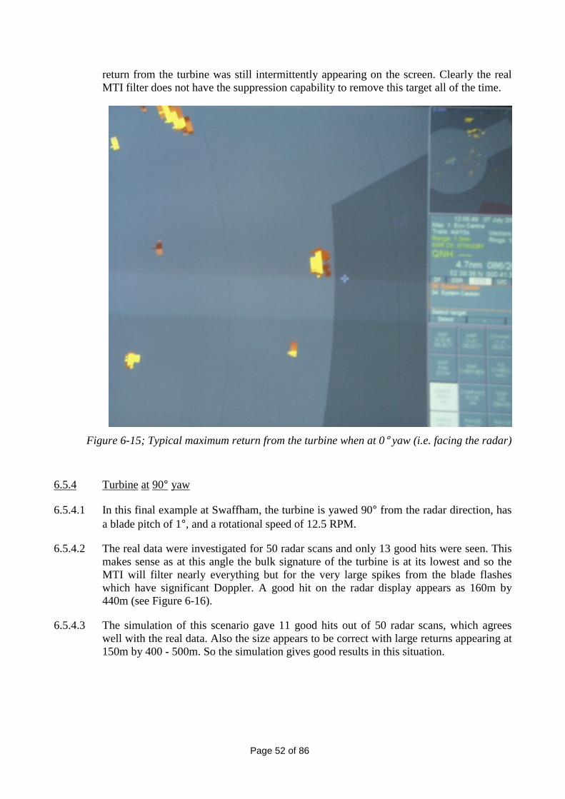
Page 52 of 86
return from the turbine was still intermittently appearing on the screen. Clearly the realMTI filter does not have the suppression capability to remove this target all of the time.
Figure 6-15; Typical maximum return from the turbine when at 0° yaw (i.e. facing the radar)
6.5.4 Turbine at 90° yaw
6.5.4.1 In this final example at Swaffham, the turbine is yawed 90° from the radar direction, hasa blade pitch of 1°, and a rotational speed of 12.5 RPM.
6.5.4.2 The real data were investigated for 50 radar scans and only 13 good hits were seen. Thismakes sense as at this angle the bulk signature of the turbine is at its lowest and so theMTI will filter nearly everything but for the very large spikes from the blade flasheswhich have significant Doppler. A good hit on the radar display appears as 160m by440m (see Figure 6-16).
6.5.4.3 The simulation of this scenario gave 11 good hits out of 50 radar scans, which agreeswell with the real data. Also the size appears to be correct with large returns appearing at150m by 400 - 500m. So the simulation gives good results in this situation.

Page 53 of 86
Figure 6-16; Results for turbine at 90° yaw when the turbine is well seen (yellow marks recent hits)for the real data (top) and WHIRL (bottom).
6.5.5 Prestwick test
6.5.5.1 No official trial took place at Prestwick. While we were on site video data were collectedfrom a PPI unit of the clutter caused by the Hare Hill wind farm. As a test of the modelwe ran a simulation of the Hare Hill site to compare with these data. Because noinformation is available of the wind turbines state while these data were recorded wehave selected a yaw angle of 40° and a rotation speed of 23 RPM. All the turbines haveexactly the same yaw and RPM and are all given random rotor start positions at the startof the simulation.
6.5.5.2 The data collected showed good correlation with the recorded data from Prestwick (seeFigure 6-17). The display at Prestwick uses different colours from Marham with yellowused for a current plot and greens used for fading older plots. This is chosen by the user.The size of the clutter on the real screen extends approximately 2300m in down rangeand 3000m in cross range. In the simulation the extent of the clutter predicted is 2500min down range and 4000m in cross range. This shows the predicted region of clutterappears wider than the recorded video. This may be due to the real turbines being at ayaw angle that is more easily filtered than the simulation. This would cause the cross-range extent to be smaller but without knowing the configuration of the turbines at thistime no certain conclusions can be drawn.
6.5.5.3 This test has demonstrated that with a multiple turbine site the simulation gives usefulinformation about radar impact.

Page 54 of 86
Figure 6-17; Comparison of the simulation of clutter produced from the Hare Hill wind farm on thePrestwick primary radar (bottom) with a real video recording (top).
6.6 Summary
6.6.1 The RCS predictions of the Swaffham turbine discussed in the previous sub-section havebeen compared to measurement data successfully. The positions of the peaks and basictrend of the measurement data were shown to be accurately predicted. Some of thepredictions are 4 to 6dB lower than the measurements, near RCS peaks but thedifferences are understood, explainable and could be corrected for.

Page 55 of 86
6.6.2 The validation of the propagation model has been limited to a simple comparisonbetween NEMESIS (used for input to WHIRL) predictions and those from anotherwidely used model, the Advanced Refractive Effects Prediction System (AREPS version2.01.2014). This is produced by the Space and Naval Warfare Systems Center, SanDiego, Atmospheric Propagation Branch. The comparison showed good agreementbetween the two models. Also NEMESIS has been extensively used and validated inprevious QinetiQ projects carried out for military customers.
6.6.3 The WHIRL model has been validated using the data recorded for a single turbine atSwaffham from the RAF Marham primary radar. The simulation agrees well with therecorded video picture for most turbine configurations. The turbine configuration thatagrees least well is when it is pointing at the radar (0° yaw).
6.6.4 To quantify the accuracy of the model we can compare the number of scans a turbine isobserved and detected by the radar with that predicted by WHIRL for each configuration.When the turbine is at 40° yaw the radar hit rate is 80%, whereas the WHIRL hit rate is73%. This is a 7% error or expressed another way the model is correct 93% of the time.At a yaw angle of 90° the radar hit rate is 26%, and the WHIRL hit rate is 24%. Thismakes the model correct 98% of the time. At 0° yaw where the agreement is not so goodthe radar hit rate is 78%, and the WHIRL hit rate is 40%. This makes the model 62%accurate at this yaw.
6.6.5 The model has been shown to be sufficiently accurate to assess the effect of a turbine onradar. The results from Prestwick, although not a proper validation of a multiple turbinesite, give encouragement and confidence that the model can give a realistic assessment ofthe clutter levels to be expected from a large wind farm.

Page 56 of 86
This page is intentionally blank