wind field retrieval from satellite radar systems
TRANSCRIPT

Wind Field Retrieval from Satellite Radar Systems
Doctoral Thesis in Physics
(September 2002)
Advisors: Dr. Ad Stoffelen and Dr. Angel Redaño
PhD program in Astronomy and Meteorology (1997-1999)

Marcos Portabella Arnús
PhD thesis
University of Barcelona, 2002.
ISBN: 90-6464-499-3
Printed by: Ponsen & Looijen BV, Amsterdam
Cover image: Sergio Ros de Mora
Cover design: Birgit van Diemen (KNMI Studio)

To my mother, Carol, Paco and Pere
“Now, there’s a man with an open mind --
you can feel the breeze from here!”
Groucho Marx

This thesis is based on the following publications:
Chapter 2
Portabella, M., and Stoffelen, A., “Characterization of residual information for SeaWinds quality control,” IEEE Trans. Geosci. Rem. Sens., accepted for publication in September 2002, Institute of Electrical and Electronics Engineers.
Chapter 3
Portabella, M., and Stoffelen, A., “Quality control and wind retrieval for SeaWinds,” Scientific report WR-2002-01, Koninklijk Nederlands Meteorologisch Instituut, The Netherlands, 2002.
Chapter 4
Portabella, M., Stoffelen, A., and Johannessen, J.A., “Toward an optimal inversion method for SAR wind retrieval,” J. Geophys. Res., vol. 107, no. C8, pp. 1-13, 2002, American Geophysical Union.
Chapter 5
Portabella, M., and Stoffelen, A., “Rain detection and quality control of SeaWinds,” J. Atm. and Ocean Techn., vol. 18, no. 7, pp. 1171-1183, 2001, American Meteorological Society.
Portabella, M., and Stoffelen, A., “A comparison of KNMI quality control and JPL rain flag for SeaWinds,” Can. Jour. of Rem. Sens., vol. 28, no. 3, pp. 424-430, 2002, Canadian Remote Sensing Society.
Other publications related to the work described in this thesis:
Portabella, M., and Stoffelen, A., “A probabilistic approach for SeaWinds data assimilation,” to be submitted to Quart. J. R. Met. Soc. in October 2002.
Portabella, M., and Stoffelen, A., “A probabilistic approach for SeaWinds data assimilation: an improvement in the nadir region,” Visiting Scientist report for the EUMETSAT NWP SAF, available at http://www.eumetsat.de/en/area4/saf/internet/, 2002.
Portabella, M., “ERS-2 SAR wind retrievals versus HIRLAM output: a two way validation-by-comparison,” ESA report EWP-1990, European Space Research and Technology Centre, Noordwijk, The Netherlands, 1998.
Portabella, M., Stoffelen, A., and De Vries, J., “Development of a SeaWinds wind product for weather forecasting,” Proc. of International Geoscience and Remote Sensing Symposium (IGARSS), vol. III, pp. 1076-1078, 2001.
Portabella, M., and Stoffelen, A., “QuikSCAT quality control: rain flag,” Proc. of Ocean Winds workshop, IFREMER, scientific topic no. 21, 2000.
Portabella, M., and Stoffelen, A., “Towards a QuikSCAT quality control indicator: rain detection,” Proc. of SPIE symposium on Remote Sensing of the Ocean and Sea Ice, vol. 4172, pp. 177-180, 2000.
Portabella, M., Stoffelen, A., and Voorrips, A., “Preliminary results in Qscat quality control: rain detection,” Proc. of QuikSCAT Cal/Val Workshop, Pasadena/Arcadia (USA), 1999.

Contents v
Contents
1 Introduction 1
1.1 Importance of sea-surface wind observations........................................................... 1
1.1.1 Meteorological observations....................................................................... 1 1.1.2 Applications of sea-surface wind observations .......................................... 3
1.2 Relation between radar backscatter and wind .......................................................... 4
1.2.1 The radar equation ...................................................................................... 4 1.2.2 Radar backscatter modulation of the sea surface........................................ 7 1.2.3 Interaction between the sea surface and the wind....................................... 9 1.2.4 The geophysical model function................................................................. 10
1.3 Remote-sensing satellite radars ................................................................................ 12
1.3.1 Scatterometers............................................................................................. 12 1.3.2 SAR............................................................................................................. 14
1.4 Wind retrieval ........................................................................................................... 17
1.4.1 Inversion problem....................................................................................... 18 1.4.2 Inversion methodology ............................................................................... 20 1.4.3 QuikSCAT problem.................................................................................... 22 1.4.4 SAR problem .............................................................................................. 23 1.4.5 Quality control ............................................................................................ 24
1.5 Aim and overview of the thesis ................................................................................ 26
2 Maximum likelihood estimation 29
2.1 Definition.................................................................................................................. 30
2.1.1 Bayesian approach ...................................................................................... 30 2.1.2 MLE optimization technique ...................................................................... 31
2.2 Cost function............................................................................................................. 32
2.2.1 Wind retrieval skill ..................................................................................... 32 2.2.2 QuikSCAT example.................................................................................... 33
2.3 Normalized residual.................................................................................................. 37
2.3.1 <MLE> for QuikSCAT............................................................................... 37
2.4 MLE characterization ............................................................................................... 42
2.4.1 Theoretical case .......................................................................................... 43

vi Wind field retrieval from satellite radar systems
2.4.2 MLE simulation .......................................................................................... 45 2.4.3 Detailed analysis of MLE differences: real versus simulated..................... 49 2.4.4 MLE influence on wind retrieval................................................................ 56
2.5 Conclusions .............................................................................................................. 58
3 Wind retrieval for determined problems: QuikSCAT case 61
3.1 Standard procedure ................................................................................................... 62
3.1.1 Inversion ..................................................................................................... 62 3.1.2 Ambiguity removal ..................................................................................... 65 3.1.3 Relevance of spatial resolution................................................................... 67
3.2 Multiple solution scheme.......................................................................................... 71
3.3 Comparison between the standard procedure and the MSS ..................................... 75
3.3.1 Statistical results ......................................................................................... 75 3.3.2 Cases ........................................................................................................... 79
3.4 Conclusions .............................................................................................................. 80
4 Wind retrieval for underdetermined problems: SAR case 83
4.1 Current wind retrieval algorithms............................................................................. 83
4.2 General approach...................................................................................................... 85
4.3 Evaluation of two SAR wind retrieval methods....................................................... 87
4.3.1 SAR and HIRLAM data ............................................................................. 87 4.3.2 SWDA+C-band method.............................................................................. 88 4.3.3 Statistical wind retrieval approach.............................................................. 95
4.4 Conclusions .............................................................................................................. 100
5 Quality control 103
5.1 KNMI quality control procedure .............................................................................. 104
5.1.1 Collocations ................................................................................................ 104 5.1.2 Rn characterization ..................................................................................... 105 5.1.3 Threshold validation ................................................................................... 110 5.1.4 Cases ........................................................................................................... 114 5.1.5 Influence of data format.............................................................................. 117
5.2 KNMI quality control versus JPL rain flag .............................................................. 121
5.2.1 JPL rain flag description............................................................................. 121 5.2.2 Comparison................................................................................................. 122 5.2.3 Cases ........................................................................................................... 125
5.3 Conclusions .............................................................................................................. 127
6 Discussion and outlook 129
6.1 Wind retrieval ........................................................................................................... 129
6.1.1 Multiple solution scheme versus general approach .................................... 129 6.1.2 QuikSCAT outer regions ............................................................................ 131 6.1.3 MLE norm .................................................................................................. 132

Contents vii
6.1.4 Data assimilation experience ...................................................................... 132
6.2 Quality control .......................................................................................................... 133
6.2.1 QuikSCAT outer regions ............................................................................ 133 6.2.2 QuikSCAT low resolution .......................................................................... 134 6.2.3 QuikSCAT rain flags .................................................................................. 135 6.2.4 SAR case..................................................................................................... 136
6.3 General aspects ......................................................................................................... 137
6.3.1 NWP data versus in-situ observations ........................................................ 137 6.3.2 Spatial resolution ........................................................................................ 138 6.3.3 Radar bands and polarizations .................................................................... 138
6.4 Outlook ..................................................................................................................... 139
A QuikSCAT data products 143
B Expected maximum likelihood estimator 145
B.1 <MLE> surface fit for the 25-km JPL-retrieved winds in HDF format ................... 145
B.2 <MLE> calculation for the 25-km JPL-retrieved winds in BUFR format ............... 146
B.3 <MLE> calculation for the 25-km KNMI-retrieved winds in BUFR format........... 149
B.4 <MLE> calculation for the 100-km KNMI-retrieved winds in BUFR format......... 149
C Inversion tuning 153
D Quality control with QSCAT-1 163
Resumen (summary in Spanish) 167
Acronyms 185
Bibliography 189
Acknowledgements 197
Curriculum vitae 199

viii Wind field retrieval from satellite radar systems
Chapter 1. Introduction 1
Chapter 1
Introduction
Most of the remote-sensing satellite radar systems can provide sea-surface wind field information, which in turn is very useful for a number of meteorological and oceanographic applications. This thesis reviews the wind retrieval procedures of such systems and explores fundamental methodology to overcome the up-to-date unresolved problems.
In this introductory chapter, the need for sea-surface wind observations, as provided by satellite radars, and the interaction between the radar signal and the wind are discussed. Then, the different satellite radar systems and the influence of their measurement geometry on wind retrieval are analysed. The aim and overview of the thesis are presented at the end of this chapter.
1.1 Importance of sea-surface wind observations
The atmospheric flow is determined by the wind field and the mass or atmospheric density field. Stoffelen (1998a) shows that pressure or temperature (mass-related magnitudes) observations alone are not sufficient to describe the atmospheric flow. Outside the Tropics, only the large-scale component of the wind field may be derived from the atmospheric pressure and temperature fields. The wind measurements are therefore necessary to define the circulation in the Tropics at all scales and elsewhere at subsynoptic scales.
1.1.1 Meteorological observations
The Global Telecommunication System (GTS) is distributing the meteorological observations of the Global Observing System (GOS) in a timely manner for many meteorological applications. The GTS conventional data include observations of pressure, temperature, humidity, wind and
2 Wind field retrieval from satellite radar systems
other parameters coming from the surface-based (ground stations, oil platforms, buoys, ships, etc.), balloon radiosonde (vertical profiles of several of these meteorological parameters) and aircraft systems. These conventional data are not enough to describe the atmospheric flow in sufficient detail (Stoffelen, 1993). Over land, there is a lack of observations in the poorly populated and/or undeveloped regions of the world. Over the oceans, the lack of observations is a more acute problem. For example, ships and aircrafts cover very limited regions of the global ocean (only traffic routes) at irregular intervals of time and space, and they tend to avoid the worst (and therefore most interesting) weather. Buoys, while of higher accuracy, have even sparser coverage (Atlas and Hoffman, 2000).
Satellites offer an effective way to provide meteorological information in these otherwise data sparse regions. There are two types of remote sensing instruments onboard satellites: passive and active.
The passive instruments measure the electromagnetic (EM) radiation coming from the Earth surface and/or its surrounding atmosphere. Several meteorological parameters can be derived from these instruments, depending on the domain of the EM spectrum (microwave, infrared, visible, etc.) where each instrument operates. For example, the thermal infrared is used by the Along Track Scanning Radiometer (ATSR) onboard the Earth Remote Sensing (ERS) satellites to retrieve sea surface temperatures; the ultraviolet, visible and near infrared is used by the Global Ozone Monitoring by Occultation of Stars (GOMOS) onboard the Environmental Satellite (ENVISAT) to retrieve ozone and other trace gases concentrations; and the infrared is used by the High-resolution Infrared Radiation Sounder (HIRS) on board the National Oceanographic and Atmospheric Administration (NOAA) polar satellites to retrieve temperature and humidity profiles of the atmosphere.
The passive instruments can also be used to retrieve winds. The emission of microwave radiation from the ocean surface depends on the surface roughness, which in turn depends on the near surface wind speed (see section 1.2.3). However, the accuracy of the retrievals decreases in the presence of clouds, and no wind direction can be derived. An example of this type of instruments is the Special Sensor Microwave Imager (SSM/I) onboard the Defense Meteorological Satellite Program (DMSP) platforms. An alternative to measure winds from passive instruments is to track clouds or humidity features from geostationary satellites (fixed with respect to an Earth location) such as Meteosat. However, it is often difficult to accurately assign a height to the features tracked.
The active instruments emit EM radiation towards the Earth and measure the properties of the signal that comes back to the instrument, after absorption, reflection or scattering by the Earth’s surface or its atmosphere. The most common measured property is the amplitude, but also the polarization, the phase or the frequency measurements are applied. Regarding the retrieval of meteorological parameters, active sensing is especially adequate for deriving winds. A good example is the Doppler Wind Lidar (DWL). The DWL emits a laser pulse towards the Earth, which is scattered in all directions by aerosol particles and molecules in the atmosphere. A small fraction of this scattering will return to the DWL. The motion of the aerosol particles in the direction of the laser beam (called line of sight, LOS) will produce a Doppler frequency shift in the return pulse. Since it is assumed that the atmospheric particles move with the wind, the LOS wind speed can be derived. Although only one component of the wind can be derived with the DWL, the instrument is very useful since it will be the first spaceborne instrument capable of retrieving wind profiles of the atmosphere. The European Space Agency (ESA) recently approved an experimental DWL mission, which is planned for launch in 2007.

Chapter 1. Introduction 3
As discussed above, the wind information is crucial to describe the atmospheric flow. Over land, despite the data voids, there is a reasonable amount of wind observations. However, the oceanic wind observing systems described up to now are either rather sparse (ships, buoys, etc.) or provide profile wind information (DWL), leading to a poor horizontal coverage, especially at the surface. Since oceans cover about 70% of the Earth’s surface, the wind observations over water are essential for a wide variety of applications (see section 1.1.2).
The radars onboard satellites are able to provide accurate sea-surface wind vector information with a high coverage (compared to conventional data). The radar is a microwave active system, which is used to observe the surface roughness. Since the sea surface roughness is driven by the wind, the latter can be inferred from radar data (see section 1.2).
A more comprehensive description of the different types of meteorological data used in the GOS can be found at the World Meteorological Organization (WMO) web site (http://www.wmo.ch).
1.1.2 Applications of sea-surface wind observations
As already discussed, the satellite radars are the main sea-surface wind information source, which is essential to describe the atmospheric flow. From the various types of satellite radars, mesoscale winds, with spatial resolutions ranging from a few km to 100 km, can be derived. Therefore, these wind observations are very useful for many meteorological and oceanographic applications.
Weather forecasting
The forecast of extreme weather events is not always satisfactory, while their consequences can have large human and economic impact. Since many weather disturbances develop over the oceans, sea surface wind observations can help to improve the prediction of the intensity and position of such disturbances.
Nowcasting, short-range forecasting and numerical weather prediction (NWP) assimilation can benefit from the sea surface wind observations. In this respect, Stoffelen and Anderson (1997a) show that the spaceborne radar winds have a beneficial impact on analyses and short-range forecast, mainly due to improvements on the sub-synoptic scales. Moreover, the impact of assimilating sea surface winds into NWP models significantly depends on the data coverage. Stoffelen and Van Beukering (1997) and Undén et al. (1997) show a much more positive impact by duplicating the sea surface wind data coverage.
Wave and Ocean modeling
Surface winds are needed to drive surface wave and surge models. A reliable wave prediction is as important as a good weather prediction for shipping activities, for example.
Ocean circulation models are driven by surface winds and heat exchange. Moreover, the surface winds are needed to calculate surface fluxes of heat, moisture and momentum at the air-sea

4 Wind field retrieval from satellite radar systems
interface. Therefore, the ocean model output is strongly related to the quality of the forcing (wind) input. Global gridded remote-sensing sea-surface winds (Bentamy et al., 2001) have been extensively used in ocean model forcing (Grima et al., 1999; Quilfen et al., 2000). The ocean circulation models play an important role, for example, in the seasonal forecasting of the El Niño southern oscillation (ENSO) or the Asian Monsoons (Latif et al., 1998).
Climate
Surface wind fields are required to validate coupled ocean-atmosphere global models, which in turn are essential to understand the Earth climate. The Tropics is a very sensitive region of our climate system. Accurate and widely available time series of near surface wind data in the Tropics would help to predict climate and climate change (Stoffelen, 1998a).
Local studies
Local wind fields, such as land-sea breezes and katabatic wind flows strongly affect the microclimate in coastal regions. They determine to a large extent the advection and dispersion of pollutants in the atmosphere and coastal waters (by generation of local wind driven currents). Since most of the world’s population lives in coastal areas and most pollutants are released into the environment near coasts, the study of these local winds is also of great relevance for environmental purposes.
The use of high-resolution sea-surface winds can be important in a number of applications, such as in semi-enclosed seas, straits, along marginal ice zones and in coastal regions.
1.2 Relation between radar backscatter and wind
The radar (transmitter) emits microwave radiation towards the Earth. This radiation, with a wavelength of typically a few centimetres, is scattered and reflected on the wind roughened sea surface such that a part of the emitted power will be detected by the radar (receiver). Only a small fraction of the radiation is absorbed by the atmosphere at the wavelengths mentioned (Rosenkranz, 1993).
1.2.1 The radar equation
In a radar system, the relation between the received power (Pr) and the transmitted power (Pt) is given by the following equation (Ulaby et al., 1982):

Chapter 1. Introduction 5
( ) rrt
ortt
r dARR
GGPP ⋅= ∫ 223
2
4
σπλ
(1.1)
where λ is the beam wavelength, G the antenna gain, R the antenna-target distance, A the effective area (radar footprint) and σ° the normalized radar cross-section (NRCS). The sub-indexes t and r stand for transmitter and receiver, respectively. Equation 1.1 represents the most generic formulation of the radar equation, which corresponds to bistatic radar. That is, the transmitter and the receiver use different antennae and can therefore be in separate locations.
In case of monostatic radar (transmitter and receiver use the same antenna), the antenna gain, antenna-target distance and effective area values are identical for the transmitter and receiver. Therefore, equation 1.1 can be re-written as:
( ) dAR
GPP
ot
r ⋅= ∫ 4
2
3
2
4
σπλ
(1.2)
If we assume that σ° does not vary over A (generally assumed over sea), we get the following expression for the averaged σ° in A:
( )t
ro
P
P
AG
R22
434
λπσ = (1.3)
However, in reality, the roughness elements on the ocean surface largely depend on the local wind condition, which in turn can exhibit large variability. Since the scattering mechanism does not linearly depend on the geophysical condition, the geophysical variability within the footprint will contribute to σ° (Stoffelen, 1998a). This is particularly acute for low winds and large footprints.
Radar footprint
The radar footprint or resolution is the spatial discrimination between signals received from different parts of an area. More specifically, the resolution is the distance between points at which the response power is half the peak-power (Pp) response. That is, the resolution is defined as the half-power width of the response. This is illustrated in Figure 1.1, where the resolution W is shown as the width between the half-power points in the response from the target sensed.
Figure 1.1 Radar definition of resolution; the half-power width (Figure 7.20 from Ulaby et al., 1982)
6 Wind field retrieval from satellite radar systems
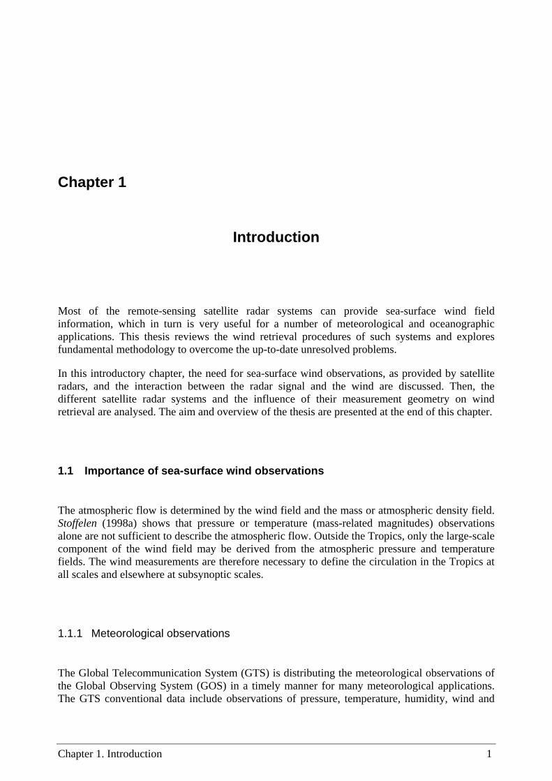
The microwave systems obtain resolution by measurement of one or more of the following quantities: angle, range, and speed. The angular discrimination is achieved by the beamwidth of the antenna. The narrower the beamwidth, the higher or “finer” the resolution (smaller the area cross-hatched in Figure 1.2a) is. The range (antenna-target direction projected onto the surface) resolution is obtained by a time-delay measurement, which is equivalent to a range measurement because of the known constant speed of the EM wave. Many different kinds of time-delay techniques may be used in radar systems, such as pulse, frequency-modulated or chirp radars (Ulaby et al., 1982). In Figure 1.2b, the crosshatched area shows the resolution resulting from the combination of the angle and the range measurements. In the case of only range measurement, that is, the antenna beam illuminates all the ground (broad beamwidth), the resolution cell would be a ring lying between the two half-power range response contours, as shown in Figure 1.2b. The speed measurement depends on the Doppler frequency shift of the received carrier frequency, which is proportional to the relative speed between the object sensed and the radar system. The geometry of a radar system travelling over the Earth is such that different points on the surface have different relative speeds. Therefore, by using the appropriate frequency filters
Figure 1.2 Methods for microwave sensing: (a) angle only, (b) angle and range, (c) angle and speed, and (d) range and speed (Figure 7.21 from Ulaby et al., 1982).

Chapter 1. Introduction 7
one can discriminate between signals from different parts of the surface of the Earth. Similar to the discussion of Figure 1.2b, Figure 1.2c shows the resolution of combining the angle and the speed measurements (cross-hatched area) and the resolution of using only the speed measurement (hyperbolic-shape strip).
The radar that does not use the speed resolution is called the real aperture radar (RAR). The scatterometer is a RAR for which a combination of range and angle resolution techniques (Figure 1.2b) is used to get a spatial resolution of typically 25-50km. The radar system that uses the combination of the range and speed discrimination (Figure 1.2d) is called the synthetic aperture radar (SAR). The SAR can have a spatial resolution up to a few meters. More detailed information about the resolution of radar systems can be found in Ulaby et al. (1982).
As discussed in section 1.3, the existing radar systems from which sea surface wind fields can be retrieved are the non-nadir looking monostatic radars (scatterometer and SAR). For such systems, the σ° or NRCS is usually called radar backscatter coefficient.
1.2.2 Radar backscatter modulation of the sea surface
As illustrated in Figure 1.3, the radar backscatter increases with the sea surface roughness. The latter modulates the radar backscatter signal in several ways. Here, we synthesise the major contributions to this modulation.
Bragg scattering
The backscatter signal from the sea surface is dominated by the so-called Bragg resonant mechanism, when using radar systems such as the scatterometer (Valenzuela, 1978) and the SAR (Hasselmann et al., 1985).
The backscatter power is proportional to the density of surface elements whose size is comparable to the incident wavelength. Therefore, the Bragg scattering is dominated by centimetre wavelength surface elements. These elements are the so-called gravity-capillary waves. They respond instantaneously to the strength of the local wind (Plant, 1982). Since the caps of these waves tend to align perpendicular to the local wind, the radar backscatter is wind direction dependent.
From a theoretical point of view, the condition for resonance of the incoming microwaves is:
θλλ
sin2
nB = (1.4)
Where λ and θ are the microwave wavelength and incidence angle respectively, λB the gravity-capillary (Bragg) wavelength, and n a positive whole number. The major contribution to the radar return is for n=1 (Valenzuela, 1978). Bragg scattering is thought to be dominant for an incidence angle range of 30° < θ < 70°.

8 Wind field retrieval from satellite radar systems
Figure 1.3 Schematic illustration of the microwave scattering and reflection at a smooth (a), rough (b), and very rough (c) ocean surface (Adopted from Figure I-5, Stoffelen, 1998a).
Specular reflection
Another mechanism to get backscatter signal from the ocean is specular reflection. The facets of the ocean that are normal to the incident microwaves will reflect the radiation back in the direction of the radar antenna. The specular reflection contribution to the backscatter signal depends on the incidence angle of the radar beam. For increasing incidence angles, the probability that a facet is oriented perpendicularly to the incident beam decreases, since the steepness of the ocean waves is limited. At the scatterometer and SAR incidence angle regime (generally, θ > 20°), the specular reflection is thought to provide a non-negligible contribution to the radar backscatter for incidence angles smaller than 30° (Stewart, 1984).

Chapter 1. Introduction 9
The orientation of the facets will generally be dependent on the surface wind speed and direction. Therefore, the contribution of the specular reflection to σ° is, as in the case of Bragg scattering, wind vector dependent.
Speckle noise and tilt modulation
At the spatial resolution of the SAR systems (up to a few meters), there are two major mechanisms that significantly increase the variability of the backscatter measurements:
• The speckle noise is a well-known problem, which occurs in a coherent system such as radars. The speckle noise is formed as a result of random phase variations in the interaction between the radar signal and the surface (Goodman, 1976). The phase variations are introduced by a single or a combination of the following effects: small-scale properties (roughness) of the surface; random motion of point scatters; and variations in the distance between the radar and the target.
• The wave modulation (tilt modulation) produces variations in the pixel intensity at such scales. That is, for ocean waves longer than the SAR resolution, the amount of specular reflection and Bragg scattering will vary according to the part of the wave which is targeted by the radar.
In order to eliminate the variability associated to these mechanisms, a practical solution is to decrease the resolution (increase the pixel size) of the SAR. By averaging the backscatter intensity over an area of 300-500 meters, the speckle noise is removed (Portabella, 1998; Lehner et al., 1998). At such scales, the variability associated to the wave modulation is also removed since the longer waves are usually between 200 and 300 meters. Therefore, by degrading the resolution of the SAR systems, the backscatter variability associated to speckle noise and wave modulation can be removed. The scatterometer systems only have the speckle type of variability but because of their large footprints (25-50 km), it is reduced to 5-10% typically.
Consequently, in terms of the mean σ° value, the scatterometer and the SAR (at 500 m resolution or lower) have similar properties (Kerbaol, 1997) and are modulated by the Bragg scattering and the specular reflection.
1.2.3 Interaction between the sea surface and the wind
As mentioned before, when the wind starts to blow over the ocean, the gravity-capillary waves are formed almost instantaneously. Part of the energy of the wind is absorbed by the ocean and transferred in space and time from the shorter waves (gravity-capillary) to the gravity (decimetric) and longer (metric or larger) waves. For increasing wind speeds, longer waves are formed. A fully developed wind sea will therefore contain a wide spectrum of waves.
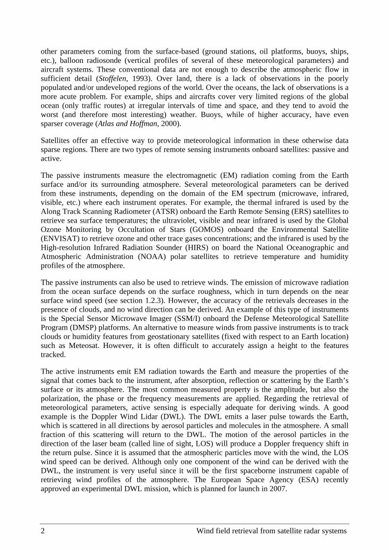
The dynamic interaction between the long and the short waves is rather complex as illustrated in Figure 1.4. The distribution of the gravity-capillary waves is modulated by the gravity and in turn the long waves. The distribution or energy density of the gravity-capillary waves is known (up to
10 Wind field retrieval from satellite radar systems
a certain degree of knowledge) to be dependent on the wind. Stoffelen (1998a) describes with some detail the theoretical relation between the wind speed and direction and the energy density of such waves.
1.2.4 The geophysical model function
As discussed in section 1.2.2, the gravity-capillary (Bragg) waves are the dominant contribution to the radar backscatter. We also know that there exists a relationship between the sea surface wind and such waves (section 1.2.3). Therefore, the centimetre-wavelength radars (scatterometer and SAR) provide in principle sea-surface wind vector information, and as such, a wind-to-backscatter relationship exists. The latter is generally referred to as the geophysical model function (GMF).
Several attempts have been made to theoretically model the GMF (Janssen et al., 1998). However, the results were not satisfactory. This is due to the fact that the ocean topography is not well understood. The interactions between long and short waves are not trivial. Phenomena such as breaking waves, foam, formation of slicks, etc., contribute in different ways, not yet understood, to the density of the gravity-capillary waves. Moreover, the EM interaction of the
Figure 1.4 Schematic illustration of the indirect modulation of short gravity-capillary waves by a long wave. (a) A simplified system consisting of a long wave (dotted), a gravity wave (dashed), and a short gravity-capillary wave (solid line). In (b) the modulation of the gravity wave by the orbital velocity of the long wave is taken into account. In (c) the modulation of the gravity-capillary waves by the gravity waves is also taken into account (Figure 5.1 from Mastenbroek, 1996).

Chapter 1. Introduction 11
radar with the complex ocean topography is not well modelled, i.e., the Bragg scattering and the specular reflection.
An alternative is to find an empirical GMF. The latter is widely used for sea surface wind retrieval from radar backscatter measurements. Several GMFs are available and tuned for different radar instruments. However the basic formulation is common to all non-nadir looking monostatic radars.
The empirically derived forward model function (GMF), which relates the state variables (wind speed and wind direction) to the observations (radar backscatter), is generally defined as:
[ ]Zo BBB )2cos()cos(1 210 φφσ ++= (1.5)
where φ is the wind direction. When the wind blows precisely in the azimuth direction of the radar beam (or view), if it blows towards the radar is referred to as upwind (φ=0°) and if it blows away from the radar is referred to as downwind (φ=180°); when it blows precisely perpendicular to the azimuth direction of the radar view, it is referred to as crosswind (φ=90° and φ=270°)., and the coefficients B0, B1 and B2 depend on the wind speed, the local incidence angle, and the polarization and frequency of the radar beam. The value of the exponent z and the number of harmonics (additional harmonics may be added to equation 1.5) depend on the tuning performed for each GMF.
The empirical GMFs were originally tuned for the different scatterometers. However, as discussed in section 1.2.2, in terms of σ°, the scatterometer and the SAR have similar properties. Therefore, a scatterometer GMF can be used to retrieve winds from SAR data, provided that the GMF is derived for the same frequency, polarization, and incidence angles used by the SAR instrument1.
Wind stress versus 10-meter wind
The reference wind used by the GMFs is the 10-meter height wind (U10). However, the energy density of the Bragg waves is actually not directly related to the surface wind but to the surface wind stress τ (momentum flux), which is a measure of the impact that the wind has on the sea surface. The relationship between τ and U10 is:
1010Uτ UCD= (1.6)
where CD is the surface drag coefficient.
Therefore, it seems more reasonable to find the empirical relationship τ-to-σ°, rather than the U10-to-σ°, and then apply equation 1.6 to derive U10. However, the CD depends on wind speed and its determination is still uncertain (compare CD parameterisations of Smith et al., 1992, with those of Donelan et al., 1993). Instead, by directly estimating the U10-to-σ°, the mean behavior of CD is taken into account implicitly. Moreover, τ observations are complicated and not widely 1 Note, however, that the sub-footprint variability, which contributes to the σ° (see section 1.2.1), depends on the footprint size. Also note from equation 1.5 that the wind direction modulation is not linear and, therefore, the sub-footprint wind direction variability will result in a small change in wind direction modulation at low winds. These effects are ignored here.

12 Wind field retrieval from satellite radar systems
available, whereas U10 observations are relatively straightforward and widely available (Stoffelen, 1998a).
Real versus neutral winds
The atmospheric stability is known to affect the surface drag (CD) and therefore the τ-to-U10 relation of equation 1.6. This will introduce some uncertainty when using real winds in the estimation of the GMF. In such cases, a mean stratification in the lowest 10 meters (as influenced by the air-sea temperature difference) at any wind velocity is taken into account. Since stability depends on the wind speed, the mentioned uncertainty is small in the case of scatterometers (large footprints). However, in the case of high resolution SAR it may still have an important effect especially when the stratification rapidly changes from stable (or neutral) to unstable. An example of GMF tuned to real 10-meter winds is the CMOD-4 (Stoffelen and Anderson, 1997b).
An alternative is to correct the measured winds (U10) to equivalent neutral winds (U10N) in the process of estimating a GMF. Since U10N is uniquely related to the stress by the corresponding drag coefficient (CDN in this case), this is equivalent to measure τ and therefore theoretically desirable. However, when estimating the GMF by using NWP model winds it is difficult to get accurate information on the atmospheric stability. Therefore, performing wind corrections with inaccurate stability information is equivalent to adding another source of error to the GMF estimation. If we use buoy data, which include accurate information on atmospheric stability, to estimate the GMF, it is still doubtful whether a correction based on local stability can be representative of the stability averaged over large radar footprints such as those from scatterometers, i.e., 25-50 km. Moreover, U10N is an oceanographic variable (remember it is equivalent to the surface stress), and therefore, once derived, it has to be corrected to U10 for further meteorological use. Without accurate information on surface stability (buoys are not everywhere), this correction is uncertain. An example of GMF tuned to neutral winds using buoy data is CMOD-Ifr (Ifremer, 1996).
1.3 Remote-sensing satellite radars
The scatterometer and SAR are the only remote-sensing satellite radar systems (up to now) capable of observing wind fields over the ocean. Therefore, this thesis will be focused on the wind retrieval problem of such systems. In this section, a brief description of the so-called monostatic non-nadir looking radars, i.e., scatterometer and SAR, is given.
1.3.1 Scatterometers
The scatterometer is a monostatic non-nadir looking RAR. As discussed in section 1.2, wind vector information can be empirically derived from it. Over the last two decades, scatterometers onboard satellites have provided very valuable sea surface wind field information. In addition to

Chapter 1. Introduction 13
the meteorological and oceanographic use of scatterometer winds, the scatterometer data are of interest in applications such as sea ice (e.g., ice edge and iceberg track monitoring) and permafrost detection, snow melt and rainforest deforestation.
In terms of the antenna geometry, the scatterometer systems can be classified as: side-looking and rotating scatterometers.
Side-looking scatterometers
The side-looking scatterometers consist of a set of fan-beam antennae with a fixed orientation, all pointing to one or both sides of the satellite flight track. The incidence angles of such radars (15° < θ < 70°) are within the Bragg scattering and specular reflection regimes.
The National Aeronautic and Space Administration (NASA) has launched two side-looking Ku-band (about 2 cm wavelength) scatterometers up to now: the Seasat-A Scatterometer System (SASS) onboard Seasat, and the NASA Scatterometer (NSCAT) onboard ADEOS-1.
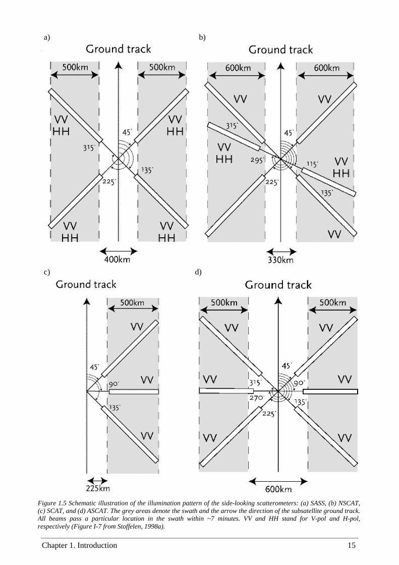
The SASS was the first satellite scatterometer. It was launched in 1978, but unfortunately failed after three months. As shown in Figure 1.5a, it had four antennae with dual polarization, horizontal (H-pol) and vertical (V-pol). At each side of the subsatellite track, the set of two antennae (fore and aft views) covered a swath of 500 km. Thus, any wind vector cell (WVC) or node (subsatellite cross-track location) of the swath is illuminated twice, first by the fore view and a few minutes later by the aft view, at two different azimuth angles (see view orientation in figure 1.5a). Since the H-pol and V-pol views were seldom operated simultaneously (Wentz et al., 1984), only two measurements are usually taken for each WVC. As it will be shown in section 1.4.1, with only two independent measurements, the wind retrieval is ambiguous. Fore more details on the Seasat mission and the SASS instrument, see Pierson (1983).
Based on the SASS experience, a follow-on instrument, NSCAT, was launched in 1996 onboard ADEOS-1, which lasted for 9 months. In comparison with SASS, a dual-polarization view (mid view) in between the fore and aft views was incorporated at each side of the swath (see Figure 1.5b); the fore and aft views were only V-pol and the swath was larger (600 km). The addition of a third view improves significantly the wind retrieval. Moreover, for H-pol the relationship between backscatter and wind differs from V-pol, and as such, H-pol provides useful complementary information, in particular on the wind direction domain. However, as we will see in section 1.4.1, the optimal orientation of the mid view would be precisely in between the fore and aft views. More NSCAT-related information can be found in JPL (1997).
In the interim between SASS and NSCAT, ESA launched two identical C-band (5.7 cm wavelength) scatterometers onboard ERS-1 (July 1991) and ERS-2 (April 1995), respectively. In contrast with SASS and NSCAT, the ERS scatterometers (SCAT) have optimal antenna geometry for wind retrieval, with the mid view precisely in between the fore and aft views (see Figure 1.5c). However, since the antennae are only V-pol (no H-pol), the wind direction retrieval is somewhat ambiguous (see section 1.4.1 and Stoffelen and Anderson, 1997c). As seen in Figure 1.5c, the SCAT illuminates only one side of the subsatellite track and its swath is 500-km wide. For more detailed information on the ERS SCAT instruments, see ESA (1993).
The Advanced scatterometer (ASCAT) due onboard METOP, which is planned for launch in late 2005, will use the same wavelength, polarization and antenna orientation as SCAT, but will be

14 Wind field retrieval from satellite radar systems
double sided (see Figure 1.5d). Therefore, ASCAT will benefit much from the knowledge gained during the ERS missions. However, the ASCAT range of incidence angles is such that the extreme outer part of the swath corresponds to incidence angles that were not available in the SCAT swath. A detailed description of ASCAT instrument and data products can be found in Figa-Saldana (2002).
Rotating scatterometers
In contrast with the side-looking scatterometers, the rotating scatterometers have a set of rotating antennae that sweep the Earth surface in a circular pattern as the satellite moves.
The SeaWinds on QuikSCAT mission (from NASA and NOAA) is a “quick recovery” mission to fill the gap created by the loss of data from NSCAT, when the ADEOS-1 satellite lost power in June 1997. It was launched in June 1999 and a similar version of the instrument (SeaWinds-2) will fly on the Japanese ADEOS-2 satellite, currently scheduled for launch in late 2002. The new-concept SeaWinds instrument is a conically scanning pencil-beam Ku-band scatterometer. It uses a rotating 1-meter dish antenna with two spot views, a H-pol view and a V-pol view at incidence angles of 46º and 54º respectively, that sweep the surface in a circular pattern (see Figure 1.6a). Due to the conical scanning, a WVC is generally viewed when looking forward (fore) and a second time when looking aft. As such, up to four views emerge: H-pol fore, H-pol aft, V-pol fore, and V-pol aft, in each WVC. The 1800-km-wide swath covers 90% of the ocean surface in 24 hours. As discussed in section 1.1.2, the data coverage is important for several applications, especially for data assimilation. In this respect, SeaWinds represents a substantial improvement compared to the side-looking scatterometers, where the largest coverage, given by NSCAT, is only half of SeaWinds coverage, i.e., 90% of the ocean surface within 48 hours. However, the wind retrieval from SeaWinds data is not trivial. In contrast with the side-looking scatterometers, the number of views and their azimuth angles vary with the subsatellite cross-track location. The wind retrieval skill will therefore depend on the area of the swath, as will be further discuss in section 1.4.3. For more detailed information on the QuikSCAT instrument and data we refer to [Spencer et al. (1997), JPL (2001), Leidner et al. (2000)].
Another concept of rotating scatterometer (RFSCAT) is currently being investigated by ESA. It consists of a rotating fan-beam scatterometer, which would sweep the Earth surface in a circular pattern (see Figure 1.6b) and would cover a wide range of incidence angles (approx. 20° < θ < 50°). The number of views and their azimuth angles vary with the subsatellite cross-track location like for SeaWinds, but due to the wide incidence angle range, generally more views are provided. For more information on the ongoing work, we refer to Lin et al. (2002).
1.3.2 SAR
The SAR is a monostatic non-nadir looking radar, which uses the range and speed (Doppler) measurements to improve resolution (see section 1.2.1). The SAR is therefore a high resolution radar, which has been used in many applications such as ocean wave modelling, sea ice detection, surface topography, land surface properties, surface soil moisture, disaster monitoring (floods,
Chapter 1. Introduction 15
a) b)
c) d)
Figure 1.5 Schematic illustration of the illumination pattern of the side-looking scatterometers: (a) SASS, (b) NSCAT, (c) SCAT, and (d) ASCAT. The grey areas denote the swath and the arrow the direction of the subsatellite ground track. All beams pass a particular location in the swath within ~7 minutes. VV and HH stand for V-pol and H-pol, respectively (Figure I-7 from Stoffelen, 1998a).

16 Wind field retrieval from satellite radar systems
a)
b) c)
Figure 1.6 Same as Figure 1.5 but for the rotating scatterometers, SeaWinds (a) [adopted from Figure I-7 of Stoffelen 1998a] and RFSCAT (b), and the SAR (c). The areas subdividing the QuikSCAT swath (plot a) are discussed in section 1.4.3.

Chapter 1. Introduction 17
earthquake, oil spills, etc.), deforestation, etc. As the scatterometer, the SAR σ° is mainly modulated (over water) by the sea-surface wind field.
During the last two decades, several SAR systems have been put into orbit onboard different satellite missions, e.g., Seasat, ERS-1, JERS-1, ERS-2, Radarsat-1 and Envisat. In terms of antenna geometry, all of them have a single-view pointing perpendicular to the flight track (see Figure 1.6c). Several parameters depend on the instrument design: the resolution (from 3 m to 1 km) the swath width (from 20 km to 500 km), the polarization (V-pol, H-pol, cross-polarization) and the frequency (C-band, Ku-band). Some of the SAR instruments can operate in different modes and therefore vary several of the mentioned parameters. For example, the Envisat SAR has the capability to change resolution, swath width and polarization using modes such as scansar, wide-swath, image, alternating polarization or global monitoring.
In order to use the SAR σ° information for wind retrieval, a comprehensive calibration is required (Scoon et al., 1996; Kerbaol, 1997). In this respect, the ERS-1 and ERS-2 SAR images can be well calibrated and therefore used for wind retrieval (Kerbaol, 1997). Such SAR instruments operate in C-band, use V-pol, have a spatial resolution of about 30 meters, a 100-km wide swath, and illuminate the Earth’s surface at a mean incidence angle of 23°. For more detailed information on the ERS SAR instruments and data, see ESA (1993).
1.4 Wind retrieval
The wind retrieval procedure for scatterometer data is schematically illustrated in Figure 1.7. A set of radar backscatter measurements (observations) in each observation cell (WVC) is inverted into a set of ambiguous wind solutions. The inversion output is then used, together with some additional information (typically from NWP models) and spatial consistency constraints, to select one of the ambiguous wind solutions as the observed wind for every WVC. This is called ambiguity removal (AR), and in contrast with the inversion, which is performed on a WVC-by-WVC basis, the AR procedure is spatially filtering many neighbouring WVCs at once.
An important aspect of wind retrieval is the quality control (QC). The goal of the QC is to detect and reject poor-quality retrieved winds. As illustrated in Figure 1.7, the output from inversion can be used for QC purposes prior to AR.
Observations Inversion Ambiguity Removal
Quality Control
Wind Field
INPUT OUTPUT
Observations Inversion Ambiguity Removal
Quality Control
Wind Field
INPUT OUTPUT
Figure 1.7 Schematic illustration of the scatterometer wind retrieval process

18 Wind field retrieval from satellite radar systems
1.4.1 Inversion problem
As discussed in section 1.2.4, the GMF (see equation 1.5) relates the radar backscatter measurements (known) to the wind speed and the wind direction (unknowns). The number of independent σ° from the same area (WVC) is therefore of particular importance for a successful inversion of the two unknowns. As shown in section 1.3, the number of views per WVC and their relative azimuth angles depend on the radar instrument design. In this section, we briefly discuss the inversion problem for different number of views and relative geometry.
a) Case with one view
Since the GMF has two unknowns (speed and direction), if only one backscatter measurement from one view is available, then the inversion problem is underdetermined. Thus, there are infinite wind speed and direction solutions, which satisfy equation 1.5, as seen from the solution curve (solid line) shown in Figure 1.8a. Moreover, the range of wind solutions is extended if we take into account the measurement noise, as denoted by the dashed and dotted curves (corresponding to a simulated ±10% noise in σ°).
b) Case with two views
Two backscatter measurements with different azimuth angles, that is, two views, should be enough to derive a unique wind-vector solution since the inversion problem should resolve two unknowns. However, because of the harmonics in the GMF, there can be up to four ambiguous solutions. This is illustrated in Figure 1.8b, where the wind solutions (see circles) correspond to the intersections of the two individual solution curves (one for each σ°). Since this is an ideal case (no noise), the solutions are always represented by curve intersections. However, if we take into account the measurement noise (positive or negative vertical shifts of the curve as shown in Figure 1.8a), sometimes there will be no intersection, thus reducing the number of solutions to up to two (even if the curves do not intersect, there will be two local minimum distances between the two curves that can be taken as solutions).
The GMF is harmonic (i.e., highly non-linear) in the wind direction domain but behaves quasi-linearly in the wind speed domain. Consequently, for two independent views, the wind speed is generally well determined (all solutions correspond to a similar wind speed value in Figure 1.8b). The degree of independence of the σ° views is given by the azimuth separation among them. Because of the harmonic wind direction dependence of the backscatter signal (clearly reflected in any solution curve of Figure 1.8), the optimal azimuth separation between two views is 90° (see Figure 1.8b). By looking only at the solid and dotted lines of Figure 1.8e, we see the effect of using two σ° views very close in azimuth (only 5° separation). Both solution curves are very close to each other (almost parallel), denoting that neither the wind direction nor the wind speed are well determined (no clear minimum distances or intersections), thus resembling the case with only one σ° view. Similar problems arise when the two views are too far in azimuth. In the extreme case where the azimuth separation is 180° (see solid and dashed lines of Figure 1.8e), the

Chapter 1. Introduction 19
only difference between the two curves is given by the upwind-downwind asymmetry (see speed value differences between the two minima in the solid or the dashed curve of Figure 1.8e). Two views can be considered independent when their azimuth separation range is [20°, 160°].
Therefore, in general, for two independent backscatter views, there will be up to four equally likely (intersection of curves) wind solutions, with varying wind speeds and very different wind directions, denoting an ambiguity problem. In case of V-pol and azimuth separation of 90°, the solution wind speeds will be very similar (as seen in Figure 1.8b).
c) Case with three or more views and good azimuth diversity
For three or more views, the inversion problem is overdetermined provided that the azimuth diversity, that is, the spread of azimuth looks among measurements (i.e., spread of views) in the WVC, is sufficiently high.
Figure 1.8c shows the inversion using 3 noise-free σ° measurements with good azimuth diversity (90° separation between fore and aft views and a mid view precisely in the middle). In this ideal case, there is a unique intersection (see right circle) of the three solution curves, potentially denoting a unique solution (the “truth” as indicated by the arrow). However, it is clearly discernible that there is another location where the lines almost intersect (see left circle), denoting a secondary solution. In reality, the measurement noise will almost always prevent any triple intersection and produce two solutions (see circles) with similar minimum curve-distance values. Thus, the inversion will result in two equally likely ambiguous wind solutions.
Figure 1.8d shows the same as Figure 1.8c but with a H-pol mid view. As mentioned before, the H-pol and V-pol backscatter are differently modulated by the wind. Thus, the incorporation of a H-pol view can help in resolving the wind direction ambiguity. In particular, comparing Figures 1.8c and 1.8d, a larger separation of the curves around the secondary solution is noticeable in the latter (see left circles), produced by the larger upwind-downwind asymmetry of the H-pol compared to the V-pol (see dashed curves). Therefore, by using a H-pol (instead of a V-pol) view, the secondary wind solution becomes less likely and consequently the inversion less ambiguous.
Generally speaking, in the presence of good azimuth diversity, there can be up to four generally well-determined wind solutions of which one or two are the most likely. This represents a clear reduction in ambiguity with respect to the two-view case.
d) Case with three or more views and poor azimuth diversity
Figure 1.8e shows the inversion using 3 noise-free σ° measurements with extremely poor azimuth diversity: two views separated 5° and a third view 180° apart. As discussed before, two σ° views separated by 5° in azimuth are not considered independent and therefore the wind retrieval is problematic. Moreover, the only difference between two views separated 180° is given by the upwind-downwind modulation of the radar backscatter. In Figure 1.8e, since all views are V-pol, the upwind-downwind modulation is almost symmetric (similar minima values in each solution curve) and the dashed line (180° apart view) is therefore very close to the other two lines, especially in the wind direction range from 150° to 300° (indicated by segment). In this ideal

20 Wind field retrieval from satellite radar systems
case, there is still a triple intersection (see arrow), denoting a unique solution. However, in the presence of noise, the curves can be indistinguishable such that this case resembles the case with only one view: almost no wind speed and direction skills.
Figure 1.8f shows the same as Figure 1.8e but with a H-pol view 180° apart. Comparing the V-pol and the H-pol solution curves (dotted lines of Figures 1.8e and 1.8f, respectively), the H-pol has a larger upwind-downwind asymmetry (as already discussed) and a smaller upwind-crosswind modulation (shown here as the speed difference between the curve maximum and minimum). Both effects contribute in Figure 1.8f to significantly separate the curves and to reduce the overlapping region to the wind direction range from 170° to 250° (indicated by segment).
By using a H-pol view, there is a gain in both the wind speed and the wind direction determination, in comparison with the three V-pol view case. However, comparing this case with the good azimuth diversity case, the loss in wind speed and direction determination is still significant.
The examples shown in this case (Figures 1.8e and 1.8f) represent the worst scenario in terms of azimuth diversity. In general, for poor azimuth diversity you can still solve certain winds with reasonable accuracy, depending on the speed and (mainly) the direction of the true wind with respect to the azimuth views, i.e., the GMF sensitivities to speed and direction changes for each view. For example, azimuth views of 80°, 100°, 170°, and 190° resolve a true wind of 60° quite well, but one of 90° badly. The inclusion of additional views will help in the determination of the wind speed and the wind direction. The more independent the additional views, the better wind vector determination, i.e., accuracy, will result.
In summary, for one view, the inversion problem is underdetermined. For two or more views, the problem is determined and, because of the low noise of satellite radar systems, the accuracy of the retrieved winds is generally high. The latter is however not true in case of poor azimuth diversity among views. Another problem of multiple-view systems is the wind direction ambiguity. This problem is most significant for two-view systems and least significant when using multiple H-pol views.
1.4.2 Inversion methodology
For two or more independent σ° views, a technique called Maximum Likelihood Estimation is used to invert winds. The Maximum Likelihood Estimation (MLE) can be interpreted as a measure of the distance between a set of n measurements and the solution lying on the two-dimensional GMF surface in a n-dimensional space (Stoffelen, 1998a). In the standard wind retrieval procedure, the minimum MLE values correspond to the wind solutions used for AR purposes. For simplicity, in section 1.4.1, the MLE is interpreted as the distance among the n single-σ° solution curves as a function of the wind direction, where the solutions correspond to the wind directions with minimum distances; the lower a minimum distance (solution) is, the larger the likelihood of this solution of being the “true” wind. As is later discussed, the MLE takes into account the measurement noise. The MLE formulation and the standard wind retrieval procedure are further discussed in chapters 2 and 3, respectively.

Chapter 1. Introduction 21
a) b)
c) d)
e) f)
Figure 1.8 The curves represent the set of wind speed and direction values, which satisfy the GMF for a single σ°measurement, produced by a wind of 8 m/s and 245° (arbitrary reference). The incidence angle of the views is 54°. The number of views and their polarizations and azimuth angles are distributed as follows: (a) one V-pol view at 45° (solid), with simulated noise in σ° (dotted and dashed correspond to +10% and –10% σ° increments, respectively); (b) two V-pol views at 45° (solid) and 135° (dotted); (c) three V-pol views at 45° (solid), 90° (dashed), and 135° (dotted); (d) same as (c) but the 90° view (dashed) being H-pol; (e) three V-pol views at 45° (solid), 50° (dotted) and 225° (dashed); (f) same as (e) but the 50° view (dotted) being H-pol. The arrows point the “truth”; the circles and segments show the possible wind solutions.

22 Wind field retrieval from satellite radar systems
For one σ° view, the inversion is underdetermined as already discussed. Therefore, additional information is needed to successfully invert winds. This will be further discussed in chapter 4.
1.4.3 QuikSCAT problem
The SeaWinds swath is divided into 76 equidistant 25km-by-25km WVCs, numbered from left to right when looking along the satellite’s propagation direction. As already mentioned, in contrast with the side-looking scatterometers, QuikSCAT has an antenna geometry, which is dependent on the WVC or node number due to its circular scans on the ocean. Figure 1.9 shows the mean azimuth separation between fore and aft views per node number, for both the outer (solid) and the inner (dotted) views. The plot shows a varying azimuth separation not only between the fore and aft views (notice that both the solid and dashed lines are far from being flat) but also between the inner and outer views (notice that the lines are not parallel), denoting an azimuth sampling (diversity) dependence on the node number. Since the outer and inner views are V-pol and H-pol, respectively, it can be easily inferred from the plot that the number of views and the polarization is also node dependent.
As discussed in section 1.4.1, the skill of the wind retrieval algorithm depends very much on the number of views and their polarization and azimuth diversity. The QuikSCAT swath is therefore
Figure 1.9 Mean azimuth separation between fore and aft views by node, for a few revolutions of HDF data; the outer view separation is in solid line and the inner view separation in dotted line.

Chapter 1. Introduction 23
subdivided in several regions, which are assigned to three different categories (see Figure 1.6a) according to the different inversion skill cases already discussed (see section 1.4.1):
• Category I corresponds to the so-called outer regions (nodes 1-8 and 69-76), where there is only V-pol outer-view information (see Figure 1.9). The inversion skill in this region corresponds to case b of section 1.4.1. At nodes 1-2 and 75-76, the azimuth separation between the fore and aft views is very small (sometimes only one view is available), thus resembling the single-view case a of section 1.4.1 and resulting in both wind speed and direction underdetermination. However, these nodes represent a very small part of the QuikSCAT swath. At the remaining outer region (nodes 3-8 and 69-74), there is enough azimuth separation between the two views (more than 20°, as seen in Figure 1.9) to consider them independent, thus resulting in a significant wind direction ambiguity.
• Category II corresponds to the so-called sweet regions of the swath (nodes 9-28 and 49-68), where there are four views (fore-inner, fore-outer, aft-inner and aft-outer) and two polarizations (H-pol and V-pol) available, with good azimuth diversity (see azimuth spreading in Figure 1.9). The inversion skill in these regions corresponds to case c of section 1.4.1 with H-pol information: the wind vector is well determined and the wind direction ambiguity is small.
• Category III corresponds to the so-called nadir region (nodes 29-48), where there also are four views and two polarizations but the fore and aft looks are nearly 180° apart and the separation between the inner and outer views is very small (see Figure 1.9), thus showing poor azimuth diversity. The inversion skill in this region corresponds to case d of section 1.4.1 with H-pol information: the wind speed and the wind direction are poorly determined.
The QuikSCAT instrument includes all the different inversion problem cases described in section 1.4.1, especially cases b, c, and d, and it is therefore of particular interest to study the wind retrieval problem. In contrast with the previously flown scatterometers, all side looking (see section 1.3.1), the QuikSCAT swath includes an area of poor azimuth diversity (nadir region), which represents a new challenge for scatterometer wind retrieval.
1.4.4 SAR problem
As discussed in section 1.2, the synthetic aperture radar (SAR) backscatter intensities (σ°) and their statistical properties contain quantitative information about the state of the sea surface roughness and therefore can be used to derive sea-surface wind information. As such, well-calibrated SAR data, e.g., ERS-1 and ERS-2 SAR instruments, can be used for wind retrieval.
Although much work has been done on the forward modelling of estimating the radar backscatter modulations from the geophysical parameters, there are fewer reports on the inverse modelling to estimate geophysical parameters from the SAR σ° modulations. The main reason for this comes from the fact that for single-view measurement instruments, such as SAR (see section 1.3.2), the wind inversion has an inherent underdetermination problem (case a of section 1.4.1). In addition,

24 Wind field retrieval from satellite radar systems
as already discussed, the relationship between σ° and the geophysical parameters is non-linear and ambiguous, further complicating the inversion.
On the other hand, C-band SAR images of the sea surface usually manifest expressions of atmospheric phenomena occurring in the marine boundary layer. Most common among these phenomena are boundary layer rolls, atmospheric convective cells, atmospheric internal gravity waves, tropical rain cells, katabatic wind flows and meteorological fronts. This has recently been documented in a series of papers published in the Special Section on Advances in Oceanography and Sea Ice Research using ERS observations (JGR, 1998) and in the EOQ (1998).
For the study of these atmospheric phenomena, SAR can provide very useful wind information. However, it is clear that additional external information needs to be used to overcome the inherent underdetermination problem of SAR wind retrieval.
1.4.5 Quality control
Radar systems such as space-borne scatterometers with extended coverage are able to provide accurate winds over the ocean surface and can potentially contribute to improve the situation for tropical and extratropical cyclone prediction (Isaksen and Stoffelen, 2000; Stoffelen and Van Beukering, 1997; Atlas et al., 2001). However, the impact of observations on weather forecast often critically depends on the Quality Control (QC) applied. For example, Rohn et al. (1998) show a positive impact of cloud motion winds on the European Centre for Medium-Range Weather Forecasts (ECMWF) model after QC, while the impact is negative without QC. The effect of QC also applies for satellite radar data. Besides their importance for NWP data assimilation, in applications such as nowcasting and short-range forecasting, the confidence of meteorologists in the satellite radar data is boosted by a better QC. Therefore, in order to successfully use satellite radar data in any of the mentioned applications, a comprehensive QC needs to be carried out in advance.
The goal of QC is to detect and reject poor-quality WVCs. Several geophysical phenomena other than wind can “contaminate” the radar observations and in turn decrease the quality of the retrieved winds. A short description of the most significant phenomena follows.
Sea ice
As previously discussed, the sea surface winds are inferred from the sea surface roughness. The wind retrieval from satellite radar systems is therefore only possible from water observations. A WVC partially or totally covered by other surfaces than water, such as land or sea ice, will contain poor or no wind information. Consequently, it is important to identify and remove such WVC from the wind retrieval process.
In contrast with the coastal lines, for which a precise description is available, the sea ice edge information is less accurate since the sea ice is continuously changing. The information used to identify sea ice areas in the radar data processing chain is often derived from satellite data, which is often insufficient for an accurate and up-to-date monitoring of the sea ice sheet changes.

Chapter 1. Introduction 25
Therefore, at high latitudes, there can be ice-contaminated WVCs, which have not been flagged as such in the data product.
Confused sea state
For a constant sea-surface wind, as the longer waves develop (see discussion on wave formation in section 1.2.3), the surface stress (and therefore CD) gradually decreases since such waves grow and move in the direction of the surface wind. The minimum surface stress corresponds to a fully developed wind sea, that is, a sea state in equilibrium with the local wind. However, Mastenbroek (1996) shows that, in general, the surface stress, characterized by the sea surface roughness, does not significantly depend on the sea state. Only in cases of confused sea state, such as in the vicinity of the center of a low-pressure system or along atmospheric front lines, where the sea is clearly not in equilibrium with the local wind, the wind retrieval is of poor quality. Moreover, in such cases, different wind fields can take part in the same WVC (e.g., imagine a front line, which separates two different wind fields, crossing the WVC), decreasing in turn the quality of the retrievals. This is of particular importance for the large scatterometer WVC, since the probability of having different wind fields in a WVC increases with the WVC size.
Rain effects
Rain is known to both attenuate and backscatter the microwave signal. Van de Hulst (1957) explains these effects. Raindrops are small compared to radar wavelengths and cause Rayleigh scattering (inversely proportional to wavelength to the fourth power). Large drops are relatively more important in the scattering and smaller wavelengths more sensitive. For example, Boukabara et al. (1999) show the variation of the signal measured by a satellite microwave radiometer with the rain rate. As the rain rate increases, the spaceborne instrument sees less and less of the radiation emitted by the surface, and increasingly sees the radiation emitted by the rainy layer that becomes optically thick due to volumetric Rayleigh scattering. For SeaWinds, at Ku-band, a dense rain cloud results in a radar cross-section corresponding to a 15-20 m/s wind.
In addition to these effects, there is a “splashing” effect. The roughness of the sea surface is increased because of splashing due to raindrops. This may increase the measured σ°, which in turn will affect the quality of wind speed (positive bias due to σ° increase) and direction (loss of anisotropy in the backscatter signal) retrievals.
Comparing Ku-band to C-band radars, the higher frequency of the former makes the rain attenuation and scattering effects about 50 times stronger. In particular, as SeaWinds operates at high incidence angles and therefore the radiation must travel a long path through the atmosphere, the problem of rain becomes acute. It is therefore very important to include a consistent QC procedure in the QuikSCAT wind retrieval process.

26 Wind field retrieval from satellite radar systems
1.5 Aim and overview of the thesis
The aim of this thesis is to review the current wind retrieval procedures of scatterometer and SAR systems, identify the most significant unresolved problems, and propose new methods (based on fundamental methodology) to overcome such problems. In this respect, the antenna geometry of the QuikSCAT nadir region presents a new problem (i.e., poor azimuth diversity) in scatterometer wind retrieval, which needs to be carefully addressed. On the other hand, although some work has been done to derive winds from SAR, the underdetermination problem of such instrument is still a major obstacle for successful wind retrieval; new ideas are therefore needed. Finally, and due to the importance of quality control in scatterometry, a QC procedure for QuikSCAT is identified as a major goal in this thesis.
In chapter 2, Maximum Likelihood Estimation, the most commonly used technique to invert winds from scatterometers, is defined and characterized. The Maximum Likelihood Estimator (MLE) is an optimization technique derived from Bayes theory, which maximizes the probability of the “true” wind by minimizing the so-called MLE cost function. The shape of the latter can in turn be used to examine the inversion problem since it provides information on the relative probability of every point (wind solution) of the cost function. In this respect, the poor azimuth diversity in the views of the QuikSCAT nadir region produces broad minima in the MLE cost function, indicating a decrease in the level of determination of the problem, compared to the steep and well defined minima of the QuikSCAT sweet regions. The QuikSCAT nadir region represents a new challenge in terms of scatterometer wind retrieval and, as such, it is identified as a region of main interest in this thesis.
Prior to investigating the wind retrieval in the QuikSCAT nadir region, the MLE behaviour is further examined. Due to non-linearities in the inversion and some misestimation of the measurement error (noise), the MLE presents some systematic dependencies. These are removed by empirically normalizing the MLE, as a function of wind speed and node number. The resulting normalized residual (Rn) is a very useful parameter for wind retrieval and quality control purposes, as demonstrated in the following chapters. Finally, the difference in the MLE distribution between different processing of the same instrument data is also examined, including a theoretical derivation of the distribution properties and a comparison between simulated and real distributions. It turns out that a reduction of the multi-dimensional space of the MLE, due to the averaging of several backscatter measurements, is the main cause for a change in the MLE distribution. Despite the distribution differences, the information content of the MLE remains almost the same as inferred from the wind retrieval scores achieved by the different data processing.
In chapter 3, the wind retrieval for determined (scatterometer) problems is revised, with special attention to the QuikSCAT nadir region. The scatterometer standard wind retrieval procedure consists of considering the MLE cost function minima as the potential (ambiguous) wind solutions that are used by the AR procedure (a spatial filter which uses background, i.e., NWP, wind information as well) to select the observed wind. In the QuikSCAT nadir region, where the cost function minima are broad, the use of the standard procedure results in inaccurate and unrealistic wind fields. This is due to the fact that the standard procedure only considers the MLE minima as potential wind solutions, ignoring all the neighbouring cost function points that are of comparable probability of being “true”. A scheme, which takes into account the information on

Chapter 1. Introduction 27
the skill of the inversion, that is, the shape of the MLE cost function, seems more suitable when the retrieval problem is less well determined. Such scheme would allow more ambiguous wind solutions (not constrained to only the cost function minima) when the retrieval problem results in broad cost function minima. A multiple solution scheme (MSS) is therefore proposed in order to overcome such inversion limitations, notably present in poor azimuth diversity areas.
The MSS uses a variational analysis AR, thus ensuring spatially consistent and meteorologically balanced retrieved fields. Moreover, the variational AR explicitly uses the relative probability of each ambiguous solution. This makes the scheme flexible enough to accept many wind solutions without the risk of oversmoothing the resulting wind field, since the less likely solutions will always be down-weighted. An empirical method, which converts the MLE values into probabilities of the “true” wind, is explained and applied for QuikSCAT.
A comparison between the standard wind retrieval and the MSS procedures is then performed, using the National Center for Environmental Prediction (NCEP) winds as background term in the variational analysis and ECMWF winds for validation. The comparison is performed at 100-km spatial resolution, since the 100-km product shows to be both less ambiguous and more accurate than the 25-km product. The MSS turns out to be more in agreement with ECMWF than the standard procedure, especially at nadir. Moreover, it shows more spatially consistent and realistic winds without removing the information content of the observations. In fact, AR results in winds with generally higher a priori probability. As such, the MSS concept is potentially beneficial for QuikSCAT data assimilation purposes in NWP.
The wind retrieval for underdetermined problems is revised in chapter 4. Single-view measurement systems such as the SAR present an inherent underdetermination problem, that is, the single-backscatter measurement, which is sensitive to both the wind speed and the wind direction, is insufficient to resolve the wind vector. However, there exist a few algorithms specially developed for SAR, which try to isolate the problem by only deriving one of the wind components. This is the case of the SAR wind direction algorithm (SWDA), which is deriving the local wind direction from the linear expressions, associated with atmospheric phenomena such as wind streaks, detected in the SAR image. Another algorithm, the scatterometer GMF, derives unambiguously the wind speed provided that the wind direction information is given. Therefore, a method, which combines the SWDA and the scatterometer GMF, can close the problem in terms of SAR wind retrieval. Such method, which provides independent wind vectors, i.e., equivalent to assuming no underdetermination, is validated against high resolution NWP data. Several problems are identified when using this method for SAR wind retrieval. The accuracy of the SWDA decreases with increasing wind streak spacing and the wind streaks show some misalignment either to the right or to the left of the “true” wind direction. Since the combined method assumes no errors, i.e., the algorithms are perfect, the reported errors in the wind direction estimation (SWDA) are directly affecting the wind speed estimation. Moreover, the wind direction cannot always be derived, denoting the inherent underdetermination problem of SAR wind retrieval.
A generalized inverse method, i.e., SAR wind retrieval algorithm (SWRA), which is based on the Bayesian approach and uses a simplistic set of assumptions, is proposed as an alternative to the current SAR wind retrieval algorithms. It acknowledges that the SAR wind retrieval is underdetermined and, as such, combines the SAR wind information (SAR term) with additional external information (background term), i.e., NWP winds, to derive the wind field taking into account that both sources of information contain errors and these are well characterized. The SWRA is validated and compared to the previous method, showing very promising results. It results in a compromise between the SAR and the NWP information. However, the SAR wind

28 Wind field retrieval from satellite radar systems
variability information is mainly added to the most sensitive wind component, i.e., the wind speed, resulting sometimes in a wind direction field close to the smooth NWP field. It is shown that by setting a more comprehensive set of assumptions, i.e., allowing the wind direction information derived from the SAR image pattern to be incorporated in the SAR term, the problem may in some cases be solved.
In chapter 5, a new QC procedure is set for QuikSCAT, in particular to screen out rain-contaminated points. It is based on the MLE and, as such, follows the QC procedures developed for NSCAT (Figa and Stoffelen, 2000) and ERS (Stoffelen, 1998a) scatterometers. The MLE indicates how well the backscatter measurements used in the retrieval of a particular wind vector fit the GMF, which is derived for fair weather conditions. The main assumption for this QC procedure is that since a large inconsistency with the GMF results in a large MLE, this indicates geophysical conditions other than those modelled by the GMF (e.g., rain, confused sea state, sea ice). A (MLE) threshold, which separates the good-quality winds from the poor-quality retrieved winds, can therefore be tuned.
A generic and empirically derived method, which uses the normalized MLE, i.e., the Rn, as QC parameter, is proposed to characterize and validate the QC procedure. The Rn results in a good QC indicator and rain detector. A Rn threshold is defined such that it maximizes the poor-quality rejections (including rain-contaminated data) and minimizes the good-quality rejections. The results show indeed the potential positive impact of assimilating QuikSCAT winds into NWP models after using the QC by Rn.
In order to improve the QC for QuikSCAT, a comparison between the above-mentioned (Royal Dutch Meteorological Institute or KNMI) QC by Rn and a rain flag developed by JPL is then performed. The KNMI QC turns out to be more effective as QC indicator, while the JPL rain flag is more effective as a rain detector. The JPL rain flag is, however, rejecting too many consistent wind data in dynamically active areas. The KNMI QC is therefore recommended. Nevertheless, in the poor azimuth diversity areas, where the JPL rain flag is able to detect some flow-inconsistent and rain-contaminated winds, which are not detected by KNMI QC, the combined use of the KNMI QC and the JPL rain flag is recommended.
In chapter 6, a general discussion on the work described in this thesis is presented. In particular, the differences and similarities of the wind retrieval methods proposed in chapters 3 and 4, that is, the MSS and the SWRA, respectively, are discussed. Both methods are based on the Bayesian approach and use some additional information, i.e., NWP winds; the main difference between them lies in the level of determination of the problem that each method is facing.
The MLE-based QC presented in chapter 5 has limited use or none when the problem is not overdetermined, that is, when there are less than three radar views, e.g., QuikSCAT outer-region and SAR cases. Alternatives to QC radar winds in such cases are presented here. Other QC issues such as the need of a QC for low-resolution winds, i.e., 50 km and 100 km, and the claim of effective rain flags in Ku-band radars are also addressed. Finally, a general outlook is presented.

Chapter 2. Maximum likelihood estimation 29
Chapter 2
Maximum Likelihood Estimation
In remote sensing, the relationship between any observation or set of observations and one or more geophysical state variables is generally represented with the following equation:
)(xy nK= (2.1)
where y is the vector of observations, x is the vector of state variables that y depends on, and the operator Kn is the so-called forward model, which relates the state variables to the observations; the subscript n reminds us that it might be non-linear. The process of deriving the best estimate of x for a given y, allowing for observation errors, is called inversion. There are several approaches for inverting remotely sensed variables, including Bayes’ theorem, exact algebraic solutions, relaxation, least squares estimation, truncated eigenvalue expansions, etc (Rodgers, 2000). The most general approach to the problem is the Bayesian approach. This approach is also used in scatterometry, where the inversion process is highly non-linear.
Several optimization techniques, which depend on the desired statistical objective, can be applied when using the Bayesian approach, including maximum likelihood, maximum posterior probability, minimum variance, minimum measurement error, etc. The maximum likelihood estimation is the most commonly used technique to invert winds in scatterometry (Pierson, 1990; Stoffelen, 1998a).
In this chapter, the MLE is defined and several of its properties, related to the inversion and quality control, are extensively examined.

30 Wind field retrieval from satellite radar systems
2.1 Definition
2.1.1 Bayesian approach
The Bayesian approach is used generally in meteorological analysis, as proposed by Lorenc (1986). He proceeded from a generic Bayesian analysis equation, expressed in terms of multi-dimensional probability distribution functions, through a fairly standard set of assumptions, to a variational equation for the “best” analysis.
The Bayes’ theorem states that the posterior probability of an event A occurring, given that event B is known to have occurred, is proportional to the prior probability of A, multiplied by the probability of B occurring given that A is known to have occurred:
)()|()|( APABPBAP ⋅∝ (2.2)
This is applicable to the inverse analysis problem. If A is the event true state (xt) and B is the event observations (yo), then equation 2.2 can be re-written as:
)()|()|( ttoot xxyyx PPP ⋅∝ (2.3)
This equation defines an Nx-dimensional Probability Distribution Function (PDF), which we shall call Pa(x), i.e., posterior probability (Rodgers, 2000), specifying all we know about the analysis. For a complete solution to the generalized problem we need to know also the accuracy of xa; this information is also contained in Pa(x).
The probability P(yo|xt) contains the uncertainty in the observation and the forward model and can be written as:
ttototo dyxyyyxyxy ⋅−⋅−=−= ∫ ))(()())(()|( nfonof kPPkPP (2.4)
where yt are the true observation values, Po represents the random observational errors and Pf the forward model errors.
The prior probability P(xt) contains our knowledge about the state x before the observations are taken. As it will be shown throughout the thesis, the definition of the prior probability is very important for solving inversion problems. Equation 2.3 can therefore be re-written as:
)())(()( tnofa PkPP xxyx o ⋅−∝ (2.5)
In using this nomenclature we have anticipated the assumption that the PDFs of Pof and P(xt) are independent, i.e., that their errors are uncorrelated, which is generally the case. If this is not the case, one should use the joint PDF instead.

Chapter 2. Maximum likelihood estimation 31
Then, as already mentioned, several optimization techniques, depending on the desired statistical objective, can be applied when using the Bayesian approach (equation 2.5). For example, the best estimate of the state xa can be the mean of Pa(x) or the maximum of Pa(x), which correspond to the minimum variance and the maximum posterior probability estimates of xa, respectively.
2.1.2 MLE optimization technique
In scatterometry, the MLE consists of maximizing Pa(x) (see equation 2.5), using no external information (other than scatterometer) in the prior probability (P(xt)) term. For example, in the case of the ERS scatterometers, the prior information in the measurement space was used in the P(xt) term to define the MLE (Stoffelen and Anderson, 1997c). For SeaWinds, no prior information about the state x is used, that is:
=)( txP constant (2.6)
For scatterometer wind retrieval, since the problem is, in general, determined (see sections 1.3 and 1.4), using no external information in the prior probability is generally valid.
Following the derivation of equation 2.5, we now need to specify the PDFs Pf and Po. A common assumption, which simplifies the solution, is that errors are Gaussian, i.e., that the PDFs are multi-dimensional Gaussian functions. In this case, equation 2.5 can be written as:
)}]({)()}({2
1exp[)( 1 xyFOxyx oo n
Tna kkP −+−−∝ − (2.7)
where O and F are the error covariance matrices of Pf and Po, respectively. Since maximizing Pa is equivalent to minimizing –ln(Pa), the MLE cost function can be written as:
)}({)()}({ 1 xyFOxy oo nT
n kkMLE −+−= − (2.8)
For scatterometers, yo contains the σ° measurements; Kn is the GMF; and x is the wind vector at 10m height. The GMF is considered perfect, i.e., F≈0, and the σ° measurements are assumed uncorrelated, i.e., O matrix is diagonal. Equation 2.8 is minimized locally, that is, in a WVC-by-WVC basis. For SeaWinds, the MLE is therefore defined as [adopted from JPL (2001)]:
( )( )∑
=
−=
N
iosi
osi
omi
kpNMLE
1
21
σσσ
(2.9)
where N is the number of measurements, σmi° is the backscatter measurement, σsi° is the backscatter simulated through the Geophysical Model Function (GMF) for different wind speed and direction trial values, and Kp(σsi°) is the measurement error variance (noise). Strictly speaking, when assuming Gaussian errors, a term ))(ln( o
siKp σ should be added to the right-hand
side of equation 2.9 but this term is not significant and, as such, is not used. [Note: the Kp is usually taken proportional to either σmi° or σsi°; the latter is chosen, following the MLE definition for QuikSCAT given by JPL.]

32 Wind field retrieval from satellite radar systems
2.2 Cost function
The MLE value represents the probability of a trial wind vector (solution) being the “true” wind, according to equation 2.3. The SeaWinds optimization technique consists of looking for the minima of equation 2.9, which represent the local solutions with maximum probability of being the “true” wind. Since it is computationally expensive to search for minimum MLE in the entire wind domain, the following procedure is usually applied in scatterometry:
• For a particular wind direction, the minimum MLE is searched as a function of wind speed, which, in contrast with wind direction, behaves quasi-linearly and a single well-determined minimum is usually found. The search is generally performed at the speed step size given by a look-up-table (LUT) (0.2 m/s for QuikSCAT).
• The same operation is repeated for every wind direction, at the step size given by the LUT (2.5° for QuikSCAT). The resulting minimum MLE as a function of wind direction is referred to as MLE cost function.
In the standard wind retrieval procedure, the MLE cost function is searched for minima. There are typically up to four minima, which are called ambiguous wind solutions. The set of (ambiguous) wind vector solutions are subsequently used for AR purposes.
2.2.1 Wind retrieval skill
The MLE (see equation 2.9) can be interpreted as a measure of the distance between a set of σmi° values and the solution σsi° set lying on the GMF surface in a transformed measurement space where each axis of the measurement space is scaled by Kp(σsi°) (Stoffelen and Anderson, 1997c). As discussed in section 1.4.2, such distance can be somehow interpreted as the distance among the single-σ° solution curves of Figure 1.8 described in section 1.4.1. The shape of the MLE cost function is then determined by the σ° modulation of any view (modulation of a single-σ° solution curve) and the relative geometry among views (“phase” shift among curves). By using the MLE cost function minima in the retrieval (standard procedure), the shape of the cost function will determine the skill of the wind retrieval.
Figure 2.1 shows an example of the MLE cost function for QuikSCAT. The diamond symbols indicate the ambiguous wind solutions detected by the inversion procedure. The shape of the minima determines the accuracy of the wind retrieval. The broader the minima (equivalent to the larger the overlapping segment in Figure 1.8), the less accurate the retrieved winds are, since we are ignoring the neighbouring wind solutions to the minima, which are of comparable probability of being the “true” wind, i.e., comparable MLE value. The depths of the minima relative to each other determine in this case the likelihood of each ambiguous solution of being the “true” wind and therefore the ambiguity or uncertainty of the system. The closer the depth of the secondary minima to that of the primary (deepest) minimum and the larger the number of (deep) minima

Chapter 2. Maximum likelihood estimation 33
(equivalent to the larger the number of clear intersections or near-intersections in Figure 1.8), the more ambiguous the wind retrieval is.
The modulation of the cost function (difference between maximum and minimum in Figure 2.1) is also important in terms of wind retrieval accuracy. It shows how unlikely the lowest likelihood points of the cost function are compared to the highest likelihood points. For example, the low GMF modulation at low winds (equivalent to the low solution curve modulation in Figure 1.8) results in a low cost function modulation. In this case, the wind direction solutions coming out of the inversion are not so meaningful anymore, since the current procedure is ignoring many cost function points of comparable probability to that of the ambiguous solutions. The low cost function modulation therefore results in low wind direction skill when using the current (i.e., standard) wind retrieval procedure1.
The MLE cost function is an output from the inversion, and as such is reflecting the inherent inversion problems. Using the minima of the MLE cost function as the only ambiguous wind solutions can lead to poor quality retrievals. As we will see in chapter 3, if we properly use the information on accuracy and ambiguity derived from the MLE cost function (inversion), the wind retrieval may improve significantly.
MLE along line of minima
0 60 120 180 240 300 360Wind Direction (degrees)
0
20
40
60
80
MLE
Figure 2.1 Example of MLE cost function for QuikSCAT node number 33. The diamond symbols indicate the locations of the minima found by the inversion procedure.
2.2.2 QuikSCAT example
As discussed in section 1.4.3, the wind retrieval performance decreases in certain regions of the QuikSCAT swath. This is an inherent problem of the QuikSCAT inversion, which is reflected in the shape of the MLE cost function.
1 Wind direction information is meteorologically less meaningful for low winds. We generally find that the wind vector error does not depend on wind speed.
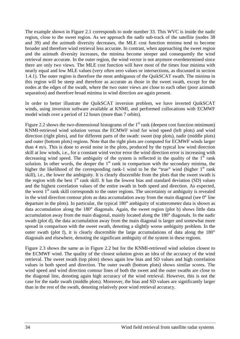
34 Wind field retrieval from satellite radar systems
The example shown in Figure 2.1 corresponds to node number 33. This WVC is inside the nadir region, close to the sweet region. As we approach the nadir sub-track of the satellite (nodes 38 and 39) and the azimuth diversity decreases, the MLE cost function minima tend to become broader and therefore wind retrieval less accurate. In contrast, when approaching the sweet region and the azimuth diversity increases, the minima become steeper and consequently the wind retrieval more accurate. In the outer region, the wind vector is not anymore overdetermined since there are only two views. The MLE cost function will have most of the times four minima with nearly equal and low MLE values (very often zero values or intersections, as discussed in section 1.4.1). The outer region is therefore the most ambiguous of the QuikSCAT swath. The minima in this region will be steep and therefore as accurate as those in the sweet swath, except for the nodes at the edges of the swath, where the two outer views are close to each other (poor azimuth separation) and therefore broad minima in wind direction are again present.
In order to better illustrate the QuikSCAT inversion problem, we have inverted QuikSCAT winds, using inversion software available at KNMI, and performed collocations with ECMWF model winds over a period of 12 hours (more than 7 orbits).
Figure 2.2 shows the two-dimensional histograms of the 1st rank (deepest cost function minimum) KNMI-retrieved wind solution versus the ECMWF wind for wind speed (left plots) and wind direction (right plots), and for different parts of the swath: sweet (top plots), nadir (middle plots) and outer (bottom plots) regions. Note that the right plots are computed for ECMWF winds larger than 4 m/s. This is done to avoid noise in the plots, produced by the typical low wind direction skill at low winds, i.e., for a constant wind vector error the wind direction error is increasing with decreasing wind speed. The ambiguity of the system is reflected in the quality of the 1st rank solution. In other words, the deeper the 1st rank in comparison with the secondary minima, the higher the likelihood of the corresponding rank-1 wind to be the “true” wind (higher 1st rank skill), i.e., the lower the ambiguity. It is clearly discernible from the plots that the sweet swath is the region with the best 1st rank skill. It has the lowest bias and standard deviation (SD) values and the highest correlation values of the entire swath in both speed and direction. As expected, the worst 1st rank skill corresponds to the outer regions. The uncertainty or ambiguity is revealed in the wind direction contour plots as data accumulation away from the main diagonal (see 0° line departure in the plots). In particular, the typical 180° ambiguity of scatterometer data is shown as data accumulation along the 180° diagonals. Again, the sweet region (plot b) shows little data accumulation away from the main diagonal, mainly located along the 180° diagonals. In the nadir swath (plot d), the data accumulation away from the main diagonal is larger and somewhat more spread in comparison with the sweet swath, denoting a slightly worse ambiguity problem. In the outer swath (plot f), it is clearly discernible the large accumulations of data along the 180° diagonals and elsewhere, denoting the significant ambiguity of the system in these regions.
Figure 2.3 shows the same as in Figure 2.2 but for the KNMI-retrieved wind solution closest to the ECMWF wind. The quality of the closest solution gives an idea of the accuracy of the wind retrieval. The sweet swath (top plots) shows again low bias and SD values and high correlation values in both speed and direction. The outer swath (bottom plots) shows similar scores. The wind speed and wind direction contour lines of both the sweet and the outer swaths are close to the diagonal line, denoting again high accuracy of the wind retrieval. However, this is not the case for the nadir swath (middle plots). Moreover, the bias and SD values are significantly larger than in the rest of the swath, denoting relatively poor wind retrieval accuracy.

Chapter 2. Maximum likelihood estimation 35
a) b) sweet swath
0 5 10 15 20Wind speed (m/s) − ECMWF
0
5
10
15
20
Win
d sp
eed
(m/s
) −
KN
MI
N= 168500mx= 7.68 my= 7.73m(y−x)= 0.04 s(y−x)= 1.61cor_xy= 0.89
sweet swath
0 90 180 270 360Wind dir (deg) − ECMWF
0
90
180
270
360
Win
d di
r (d
eg)
− K
NM
I
N= 138412mx= 177.23 my= 177.47m(y−x)= 0.24 s(y−x)= 48.98cor_xy= 0.90
c) d) nadir swath
0 5 10 15 20Wind speed (m/s) − ECMWF
0
5
10
15
20
Win
d sp
eed
(m/s
) −
KN
MI
N= 94521mx= 7.57 my= 7.66m(y−x)= 0.09 s(y−x)= 1.70cor_xy= 0.88
nadir swath
0 90 180 270 360Wind dir (deg) − ECMWF
0
90
180
270
360
Win
d di
r (d
eg)
− K
NM
I
N= 75969mx= 190.13 my= 191.61m(y−x)= 1.48 s(y−x)= 56.34cor_xy= 0.88
e) f) outer swath
0 5 10 15 20Wind speed (m/s) − ECMWF
0
5
10
15
20
Win
d sp
eed
(m/s
) −
KN
MI
N= 57558mx= 7.51 my= 7.85m(y−x)= 0.35 s(y−x)= 2.27cor_xy= 0.83
outer swath
0 90 180 270 360Wind dir (deg) − ECMWF
0
90
180
270
360
Win
d di
r (d
eg)
− K
NM
I
N= 45712mx= 213.11 my= 214.50m(y−x)= 1.39 s(y−x)= 106.86cor_xy= 0.64
Figure 2.2 Two-dimensional histogram of the 1st rank KNMI-retrieved wind solution versus ECMWF wind in the different parts of the swath: the sweet (top plots), the nadir (middle plots) and the outer (bottom plots) regions. The left plots correspond to wind speed (bins of 0.4 m/s) and the right plots to wind direction (bins of 2.5°). The latter are computed for ECMWF winds larger than 4 m/s. N is the number of data; mx and my are the mean values along the xand y axis, respectively; m(y-x) and s(y-x) are the bias and the standard deviation with respect to the diagonal, respectively; and cor_xy is the correlation value between the x- and y-axis distributions. The contour lines are in logarithmic scale: each step is a factor of 2 and the lowest level (outer-most contour line) is at N/8000 data points.
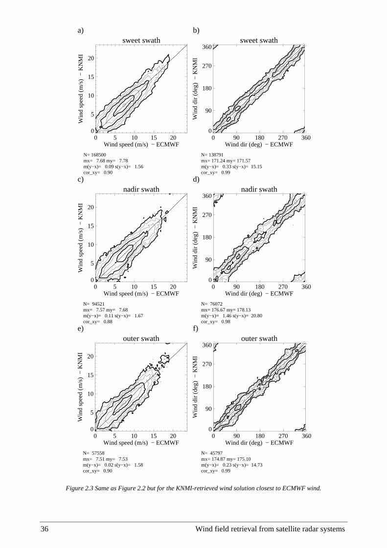
36 Wind field retrieval from satellite radar systems
a) b) sweet swath
0 5 10 15 20Wind speed (m/s) − ECMWF
0
5
10
15
20
Win
d sp
eed
(m/s
) −
KN
MI
N= 168500mx= 7.68 my= 7.78m(y−x)= 0.09 s(y−x)= 1.56cor_xy= 0.90
sweet swath
0 90 180 270 360Wind dir (deg) − ECMWF
0
90
180
270
360
Win
d di
r (d
eg)
− K
NM
I
N= 138791mx= 171.24 my= 171.57m(y−x)= 0.33 s(y−x)= 15.15cor_xy= 0.99
c) d) nadir swath
0 5 10 15 20Wind speed (m/s) − ECMWF
0
5
10
15
20
Win
d sp
eed
(m/s
) −
KN
MI
N= 94521mx= 7.57 my= 7.68m(y−x)= 0.11 s(y−x)= 1.67cor_xy= 0.88
nadir swath
0 90 180 270 360Wind dir (deg) − ECMWF
0
90
180
270
360W
ind
dir
(deg
) −
KN
MI
N= 76072mx= 176.67 my= 178.13m(y−x)= 1.46 s(y−x)= 20.80cor_xy= 0.98
e) f) outer swath
0 5 10 15 20Wind speed (m/s) − ECMWF
0
5
10
15
20
Win
d sp
eed
(m/s
) −
KN
MI
N= 57558mx= 7.51 my= 7.53m(y−x)= 0.02 s(y−x)= 1.58cor_xy= 0.90
outer swath
0 90 180 270 360Wind dir (deg) − ECMWF
0
90
180
270
360
Win
d di
r (d
eg)
− K
NM
I
N= 45797mx= 174.87 my= 175.10m(y−x)= 0.23 s(y−x)= 14.73cor_xy= 0.99
Figure 2.3 Same as Figure 2.2 but for the KNMI-retrieved wind solution closest to ECMWF wind.

Chapter 2. Maximum likelihood estimation 37
In summary, as seen in Figures 2.2 and 2.3, the sweet regions show the best wind retrieval skill of the QuikSCAT swath, in terms of ambiguity and accuracy. Although there is a significant ambiguity problem in the outer swath, its accuracy is comparable to that of the sweet swath1. The wind retrieval accuracy in the nadir region is significantly poorer compared to the outer and sweet regions of the QuikSCAT swath.
2.3 Normalized residual
The MLE represents a distance, which is “normalized” by the measurement error variance or noise (see equation 2.9). In this respect, the MLE should behave uniformly across the swath (node number) and over any wind condition. However, it often presents some unwanted dependencies, and the main reason for this is that the measurement noise is misestimated (a more detailed analysis on these dependencies can be found in section 2.4.3). In order to avoid this problem, for a given wind and node number, an expected MLE value can be estimated, and used to normalize the MLE in the following way:
Rn = MLE / <MLE> (2.10)
where the MLE value represents any point of the cost function for a particular WVC, and <MLE> is the expected MLE for that WVC (node number) and wind condition.
Note that we are not trying to change the relative weights of equation 2.9 but rather to provide an averaged normalization of the MLE. In other words, we do not intend to optimise the inversion, i.e., change the MLE formula, since we believe that equation 2.9 is already working reasonably well for such purpose; we rather want to define a more stable parameter which may be useful for other applications. As we will see in chapters 3 and 5, the Rn (see equation 2.10) is a very useful parameter for wind retrieval and QC purposes, respectively.
2.3.1 <MLE> for QuikSCAT
The purpose of the <MLE> is to compensate the misestimation of the measurement noise in order to correct the MLE dependencies. Therefore, an accurate knowledge of the instrument and geophysical (O+F in equation 2.8) noise is needed. In this respect, Figa and Stoffelen (2000) used an instrument error model derived by Cavanié (1997) to compute the <MLE> of the NSCAT Rn parameter.
Since there is no instrument error model available for QuikSCAT, an alternative method has to be sought. As discussed in section 1.4.1, in an ideal case (no noise), the single-σ° solution curves do always intersect. In reality, and because of the measurement noise, the solution curves may not
1 Note that a feature of the closest is that the more solutions are available, the better the apparent quality. However, it is clear that quality degrades with the number of solutions. The outer swath results are therefore too optimistic, since the outer swath represents more solutions (typically four) than the rest of the swath (on average, between two and three).
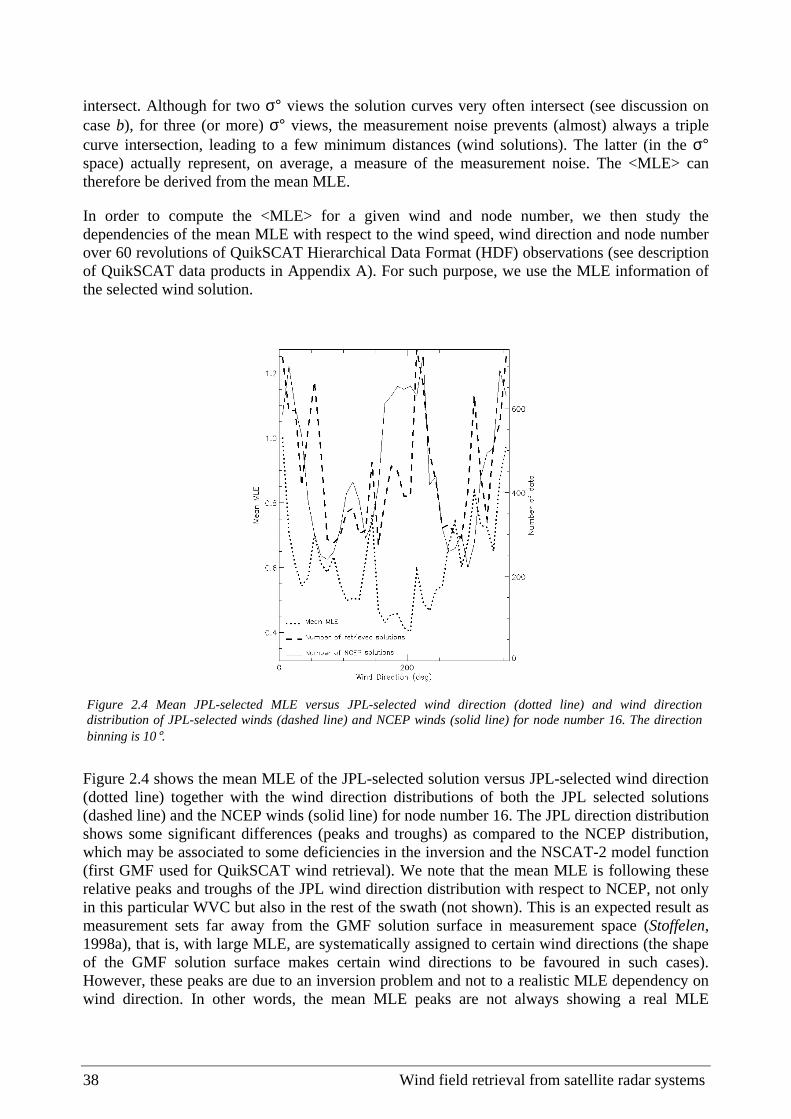
38 Wind field retrieval from satellite radar systems
intersect. Although for two σ° views the solution curves very often intersect (see discussion on case b), for three (or more) σ° views, the measurement noise prevents (almost) always a triple curve intersection, leading to a few minimum distances (wind solutions). The latter (in the σ° space) actually represent, on average, a measure of the measurement noise. The <MLE> can therefore be derived from the mean MLE.
In order to compute the <MLE> for a given wind and node number, we then study the dependencies of the mean MLE with respect to the wind speed, wind direction and node number over 60 revolutions of QuikSCAT Hierarchical Data Format (HDF) observations (see description of QuikSCAT data products in Appendix A). For such purpose, we use the MLE information of the selected wind solution.
Figure 2.4 shows the mean MLE of the JPL-selected solution versus JPL-selected wind direction (dotted line) together with the wind direction distributions of both the JPL selected solutions (dashed line) and the NCEP winds (solid line) for node number 16. The JPL direction distribution shows some significant differences (peaks and troughs) as compared to the NCEP distribution, which may be associated to some deficiencies in the inversion and the NSCAT-2 model function (first GMF used for QuikSCAT wind retrieval). We note that the mean MLE is following these relative peaks and troughs of the JPL wind direction distribution with respect to NCEP, not only in this particular WVC but also in the rest of the swath (not shown). This is an expected result as measurement sets far away from the GMF solution surface in measurement space (Stoffelen, 1998a), that is, with large MLE, are systematically assigned to certain wind directions (the shape of the GMF solution surface makes certain wind directions to be favoured in such cases). However, these peaks are due to an inversion problem and not to a realistic MLE dependency on wind direction. In other words, the mean MLE peaks are not always showing a real MLE
Figure 2.4 Mean JPL-selected MLE versus JPL-selected wind direction (dotted line) and wind direction distribution of JPL-selected winds (dashed line) and NCEP winds (solid line) for node number 16. The direction binning is 10°.

Chapter 2. Maximum likelihood estimation 39
dependency on wind direction but just some artificial accumulation of wind direction solutions due to some deficiencies in the inversion. Therefore, we discard the wind direction dependency when computing the <MLE>.
As such, <MLE> is computed as a function of wind speed and node number. The method to compute <MLE> is as follows:
• We compute the mean MLE of the JPL-selected solution with respect to the JPL-selected wind speed and the node number for the 60 revolutions of HDF data. Figure 2.5a shows a 3D plot of this mean MLE. The surface is a bit noisy, which is mainly due to geophysical effects such as rain, which we want to discard from wind retrieval. At high wind speeds additional noise is present due to the small amount of data we get at these speeds and node numbers.
• In order to filter the noise on the surface, we set up an iterative process which consists in rejecting the MLEs which are at least two times higher than the mean MLE for that particular wind speed and node number, and we compute again the mean MLE surface. Then, we start the rejection process again in an iterative mode until it converges (no more rejections). The process converges very rapidly after two iterations and the number of data rejected in each speed and node bin is very small (up to 7% in some high-speed bins). This gives faith in the noise filtering method as it shows that only the tail of the MLE distribution is cut in each bin, corresponding to geophysical anomalies. The resulting surface is shown in Figure 2.5b. The peaks have disappeared in general and at high speeds the surface is much smoothed. In order to show the consistency of this filtering procedure, we show the contour plots of both mean MLE surfaces (before and after filtering) in Figure 2.6. It is clearly discernible that the shape of the surface remains the same and only the noise has been removed.
• In order to extrapolate to high wind speeds, we fit a two-dimensional function to the filtered surface in a very simple way (see Appendix B.1). The function is only fit in the inner swath (nodes 9 to 68) and extrapolated for the outer swath (nodes 1 to 8 and 69 to 76) (see discussion below). The result of the fitting is shown in Figure 2.7. The 3D surface is the expected MLE and compares well to the computed mean MLE in the inner part of the swath.
As discussed in section 1.4.1, for two σ° views, the solution curves intersect (equivalent to null MLE value) very often regardless of the measurement noise. In such a case, i.e., outer regions, the MLE is not a good noise indicator. However, as it is clearly discernible from Figure 2.7, the mean MLE of the inner swath can be extrapolated to the outer regions, thus providing Rn computation for the entire QuikSCAT swath.
In this section, we have shown a method to compute the <MLE>, and therefore the Rn, for QuikSCAT. For such purpose, we use the “selected” solution information available in the JPL HDF data product. However, the <MLE> can be computed from: another inversion (e.g., KNMI inversion); another data format (e.g., BUFR); or another cost function solution (e.g., 1st rank). In this thesis, we will use the Rn for different purposes, which in turn will require different <MLE> surfaces. The computation of the latter can be found in Appendix B.
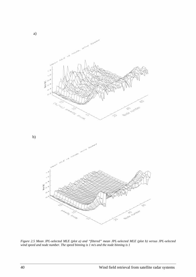
40 Wind field retrieval from satellite radar systems
a)
b)
Figure 2.5 Mean JPL-selected MLE (plot a) and “filtered” mean JPL-selected MLE (plot b) versus JPL-selected wind speed and node number. The speed binning is 1 m/s and the node binning is 1

Chapter 2. Maximum likelihood estimation 41
a) b)
Figure 2.6 Contour plots of Figure 2.5a (plot a) and 2.5b (plot b).
Figure 2.7 Expected MLE versus wind speed and node number. The speed binning is 1 m/s and the node binning is 1.

42 Wind field retrieval from satellite radar systems
2.4 MLE characterization
For QuikSCAT, the data are distributed in two different formats, according to time delay constraints: on the one hand, a complete data product, which usually takes a few weeks to be delivered and is used for broad scientific purposes; on the other hand, a near-real time (NRT) product, which takes a few hours to be delivered, contains somehow reduced information (aggregated data) compared to the former product, and is used for operational purposes (e.g., data assimilation). The former is the Hierarchical Data Format (HDF) and the latter is the Binary Universal Format Representation (BUFR). A full description of the HDF and BUFR data products can be found in JPL (2001) and Leidner et al. (2000), respectively.
Figure 2.8 shows the contour plot of the two-dimensional histogram of the BUFR MLE versus the HDF MLE for QuikSCAT. [Note: in this section, the MLE of the 1st rank solution from the QuikSCAT sweet swath nodes is used; the NSCAT-2 GMF is used in the MLE computation]. The plot shows only small correlation (around 0.5) between both MLE distributions. Moreover, the mean BUFR MLE value (0.28) is significantly smaller than the mean HDF value (0.57).
It is clear from these results that the MLE distributions of both formats are significantly different. Since the MLE information is essential for wind retrieval and QC purposes (see chapters 3 and 5, respectively, for further discussion), it seems relevant at this stage to try to understand these differences and their implications for scatterometry. We therefore perform a comprehensive characterization of the MLE.
MLE HISTOGRAM
0.0 0.5 1.0 1.5 2.0 2.5HDF MLE
0.0
0.5
1.0
1.5
2.0
2.5
BU
FR
MLE
N=1114381
mx= 0.57 my= 0.28
m(y−x)= −0.30 s(y−x)= 0.46
cor_xy= 0.55
Figure 2.8 Contour plot of the two-dimensional histogram of the BUFR MLE versus the HDF MLE. The legend and the contour lines are the same as in Figure 2.2 (the lowest contour level is, in this case, at N/4000 data points).

Chapter 2. Maximum likelihood estimation 43
Appendix A describes the main differences between HDF and BUFR, in terms of the σ° information. In summary, the BUFR σ° is an average of the different HDF σ° measurements per view. From a theoretical point of view, the MLE distribution characteristics may change just by taking a different number of σ° in the MLE computation. In this section, we show this with a simple example. Then, a simulation is performed to bridge the gap between theory and reality. Finally, the impact of the different (HDF and BUFR) MLE behavior on wind retrieval is examined.
2.4.1 Theoretical case
As discussed in section 2.2.1, the MLE is a distance between the σ° measurements and the solution lying on the GMF surface, more precisely a squared distance (see equation 2.9). The following case corresponds to a simplified version of the MLE, which uses the following set of assumptions:
1) Typically for SeaWinds, HDF contains N>4 σ° per WVC while BUFR contains M=4 σ° per WVC in the sweet swath. Therefore, the MLE is computed for HDF in a higher dimensional measurement space than for BUFR. In this example we simplify the problem assuming N=2 and M=1.
2) The truth or solution lies in the origin of our measurement space for simplicity.
3) Since in scatterometry the errors are considered Gaussian, we consider pairs of measurements (x,y) in the N(=2)-dimensional space as Gaussian distributed points around the origin (solution). Therefore, we use the following two-dimensional Gaussian PDF (Probability Density Function):
( )dxdyedxdyyxp
yx2
22
2
1
22
1),( σ
πσ
+−= , (2.11)
where the SD in both axis is assumed identical, i.e., σ =σx=σy.
4) For simplicity, we also assume constant Kp noise values for both HDF and BUFR. As such, the MLE is equivalent to a squared distance to the origin weighted by a constant factor. Moreover, this assumption is important since it will allow us to show the significant change between the mentioned MLE distributions just by setting N>M.
Mathematical demonstration
In order to show the difference between two distributions, we use the following mathematical definitions:
• The mean or expected value of a function f(x,y) is defined in terms of the PDF p(x,y) by
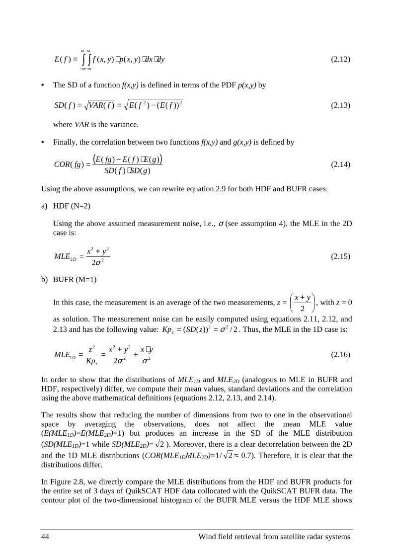
44 Wind field retrieval from satellite radar systems
∫ ∫∞
∞−
∞
∞−
⋅⋅⋅= dydxyxpyxffE ),(),()( (2.12)
• The SD of a function f(x,y) is defined in terms of the PDF p(x,y) by
22 ))(()()()( fEfEfVARfSD −== (2.13)
where VAR is the variance.
• Finally, the correlation between two functions f(x,y) and g(x,y) is defined by
( ))()(
)()()()(
gSDfSD
gEfEfgEfgCOR
⋅⋅−= (2.14)
Using the above assumptions, we can rewrite equation 2.9 for both HDF and BUFR cases:
a) HDF (N=2)
Using the above assumed measurement noise, i.e., σ (see assumption 4), the MLE in the 2D case is:
2
22
2 2σyx
MLE D
+= (2.15)
b) BUFR (M=1)
In this case, the measurement is an average of the two measurements, z =
+2
yx, with z = 0
as solution. The measurement noise can be easily computed using equations 2.11, 2.12, and 2.13 and has the following value: 2/))(( 22 σ== zSDKpz . Thus, the MLE in the 1D case is:
22
222
1 2 σσyxyx
Kp
zMLE
zD
⋅++== (2.16)
In order to show that the distributions of MLE1D and MLE2D (analogous to MLE in BUFR and HDF, respectively) differ, we compute their mean values, standard deviations and the correlation using the above mathematical definitions (equations 2.12, 2.13, and 2.14).
The results show that reducing the number of dimensions from two to one in the observational space by averaging the observations, does not affect the mean MLE value (E(MLE1D)=E(MLE2D)=1) but produces an increase in the SD of the MLE distribution (SD(MLE1D)=1 while SD(MLE2D)= 2 ). Moreover, there is a clear decorrelation between the 2D
and the 1D MLE distributions (COR(MLE1DMLE2D)= 2/1 ≈ 0.7). Therefore, it is clear that the distributions differ.
In Figure 2.8, we directly compare the MLE distributions from the HDF and BUFR products for the entire set of 3 days of QuikSCAT HDF data collocated with the QuikSCAT BUFR data. The contour plot of the two-dimensional histogram of the BUFR MLE versus the HDF MLE shows

Chapter 2. Maximum likelihood estimation 45
indeed small correlation between both MLE distributions, as presented in the introduction. However, the results differ somewhat from the theoretical example. The correlation is smaller in the real case and the ratio between the mean values of HDF and BUFR distributions is 1 in the case of the theoretical example while 2 in the real case where the mean BUFR MLE value (0.28) is substantially smaller than the mean HDF value (0.57). This can be expected, since the theoretical example is just a simplification of the problem as discussed above. In order to understand the real results in more detail, a simulation is needed.
2.4.2 MLE Simulation
In the simple example that we theoretically solve in Section 2.4.1, we show that the small correlation between HDF and BUFR MLE distributions is due to the σ° averaging, assuming two measurements for HDF and one for BUFR. However, in the real case, where HDF contains more than four measurements and BUFR typically four, the results, although similar, present some differences with respect to the theoretical case. In particular, the correlation is significantly smaller (0.5) compared to the simple theoretical example (0.7).
In this section, we simulate HDF and BUFR MLEs, assuming a realistic number of measurements for both sets. First, the simulation is constrained to the most important assumptions used in the theoretical case to show that the theoretical demonstration can be extrapolated to the real case by using a larger number of σ° in both HDF and BUFR products. Then, a more realistic simulation is compared to the real distribution. Finally, we simulate the effects of varying the number of σ° on the MLE distributions.
2.4.2.1 Simulation procedure We use the JPL-selected winds of the BUFR files as truth to simulate two sets of measurements. The first set simulates the HDF product, using realistic noise values and number of measurements per view. Then, similar to the real data, these measurements are averaged per view to generate the second set which simulates the BUFR product. The more HDF observations per view in a particular WVC that we simulate, the larger the measurement noise that we assume for each individual measurement, such that the information content is the same in each simulated HDF and BUFR WVC. Once we have simulated both sets of measurements, we invert them, using equation 2.9, to derive the simulated MLE.
Number of σº
In order to adequately simulate both products we have to use a realistic number of σ° per WVC. In the case of the HDF simulation, we produce a variable number of measurements depending on the WVC number and view.

46 Wind field retrieval from satellite radar systems
Figure 2.9 shows the histogram of the number of measurements per WVC and view for one day of HDF data. [Note that because of symmetry, both the fore-view and the aft-view histograms are identical; therefore, only one of them is shown in the Figure]. Figure 2.9a corresponds to WVC number 12 and Figure 2.9b to WVC number 55. It is clear from the different distributions of Figures 2.9a and 2.9b that the number of measurements in HDF varies from one WVC to another. Moreover, these distributions are broad, indicating that the number of measurements is varying considerably in each WVC as well. However, to simplify the simulation, we have chosen the number of σº corresponding to the peak of each distribution as the fixed value to represent the number of σº for each particular WVC and view.
As explained above, the BUFR measurements are produced by averaging the HDF measurements per view. Therefore, the number of σº in BUFR will depend on the number of views in HDF. Since we perform this simulation in the sweet parts of the swath, we use a constant number of four σ° per WVC for BUFR.
a) b)
Figure 2.9 Normalized histogram of the number of σ° measurements for WVC numbers 12 (plot a) and 55 (plot b). The solid line corresponds to one of the inner swath views (fore or aft views have the same distributions) and the dotted line to one of the outer swath views.
2.4.2.2 Simulation results
In order to provide a realistic simulation, we use the Kp and the wind distributions as provided in the JPL product together with the realistic number of measurements for HDF and BUFR computed in section 2.4.2.1
Figure 2.10 shows the contour plot of the two-dimensional histogram of the simulated BUFR MLE versus the simulated HDF MLE. Although the distribution differs somewhat from the real case (Figure 2.8), it is clear that we have successfully reproduced the same small correlation (about 0.5 in both cases) by simply assuming a different number of measurements (more σº in HDF than BUFR). The remaining differences between the simulated and the real distributions, which can be explained by many issues, are analysed in detail in section 2.4.3. Nevertheless, it is clear from the results that the simulation is a good reflection of reality. Therefore, since averaging
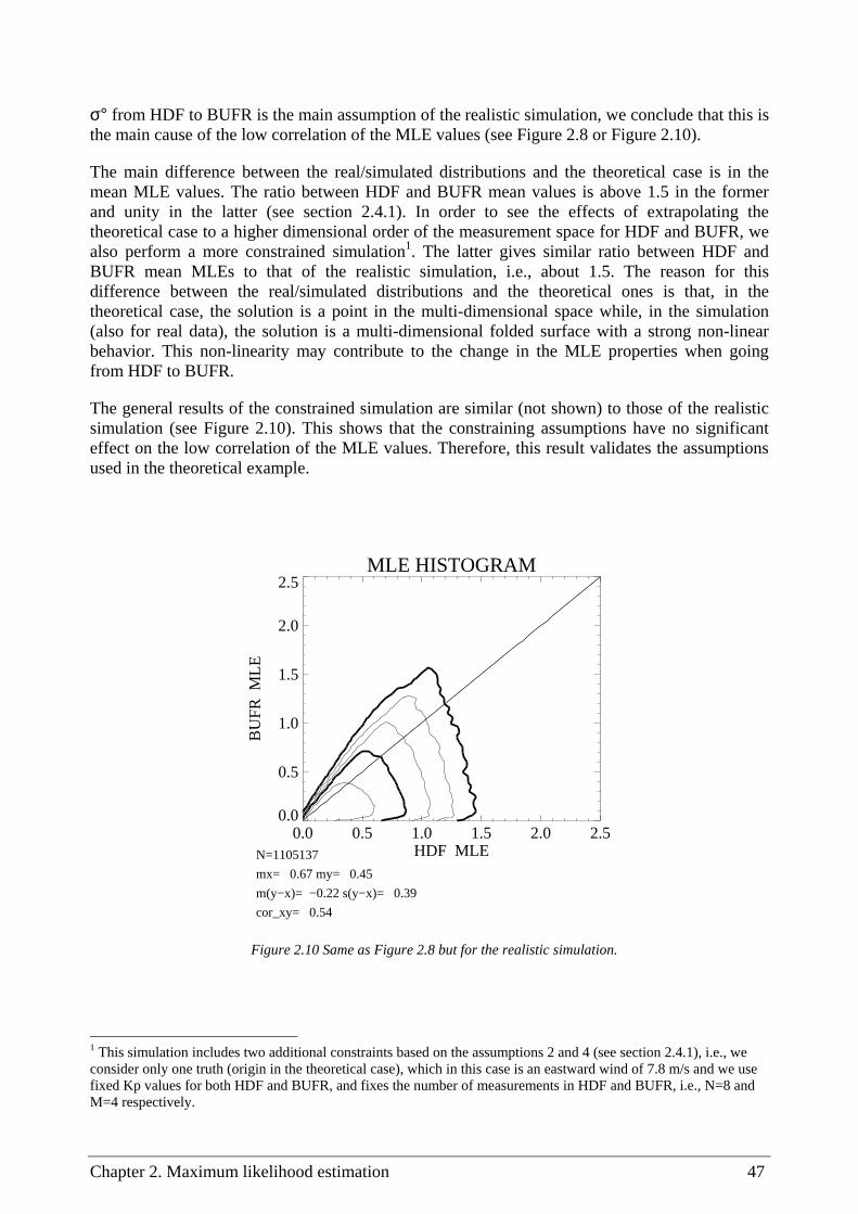
Chapter 2. Maximum likelihood estimation 47
σ° from HDF to BUFR is the main assumption of the realistic simulation, we conclude that this is the main cause of the low correlation of the MLE values (see Figure 2.8 or Figure 2.10).
The main difference between the real/simulated distributions and the theoretical case is in the mean MLE values. The ratio between HDF and BUFR mean values is above 1.5 in the former and unity in the latter (see section 2.4.1). In order to see the effects of extrapolating the theoretical case to a higher dimensional order of the measurement space for HDF and BUFR, we also perform a more constrained simulation1. The latter gives similar ratio between HDF and BUFR mean MLEs to that of the realistic simulation, i.e., about 1.5. The reason for this difference between the real/simulated distributions and the theoretical ones is that, in the theoretical case, the solution is a point in the multi-dimensional space while, in the simulation (also for real data), the solution is a multi-dimensional folded surface with a strong non-linear behavior. This non-linearity may contribute to the change in the MLE properties when going from HDF to BUFR.
The general results of the constrained simulation are similar (not shown) to those of the realistic simulation (see Figure 2.10). This shows that the constraining assumptions have no significant effect on the low correlation of the MLE values. Therefore, this result validates the assumptions used in the theoretical example.
1 This simulation includes two additional constraints based on the assumptions 2 and 4 (see section 2.4.1), i.e., we consider only one truth (origin in the theoretical case), which in this case is an eastward wind of 7.8 m/s and we use fixed Kp values for both HDF and BUFR, and fixes the number of measurements in HDF and BUFR, i.e., N=8 and M=4 respectively.
MLE HISTOGRAM
0.0 0.5 1.0 1.5 2.0 2.5HDF MLE
0.0
0.5
1.0
1.5
2.0
2.5
BU
FR
MLE
N=1105137
mx= 0.67 my= 0.45
m(y−x)= −0.22 s(y−x)= 0.39
cor_xy= 0.54
Figure 2.10 Same as Figure 2.8 but for the realistic simulation.

48 Wind field retrieval from satellite radar systems
MLE distribution dependence on number of σº
Figure 2.11 is similar to Figure 2.10. We use the same simulation procedure but in this case we fix the number of σ° used in the simulated HDF instead of using a realistic number. In the case of fixing the number of HDF measurements to 5 (plot a), one view has two σ° measurements and the rest of the views have only one each. In the case of 6 σ° measurements (plot b), two views have two measurements each and the other two views have only one measurement each. Analogous explanation goes for the cases of 7 (plot c) and 8 (plot d) measurements. [Note that the different combinations of measurements / views (e.g., in the case of 5 σ°, you may use two measurements for the fore inner, the fore outer, the aft inner or the aft outer view) do not affect
a) b) MLE HISTOGRAM
0.0 0.5 1.0 1.5 2.0 2.5HDF MLE
0.0
0.5
1.0
1.5
2.0
2.5
BU
FR
MLE
N= 24927
mx= 0.54 my= 0.45
m(y−x)= −0.09 s(y−x)= 0.28
cor_xy= 0.78
MLE HISTOGRAM
0.0 0.5 1.0 1.5 2.0 2.5HDF MLE
0.0
0.5
1.0
1.5
2.0
2.5B
UF
R M
LE
N= 24927
mx= 0.59 my= 0.44
m(y−x)= −0.15 s(y−x)= 0.34
cor_xy= 0.66
c) d) MLE HISTOGRAM
0.0 0.5 1.0 1.5 2.0 2.5HDF MLE
0.0
0.5
1.0
1.5
2.0
2.5
BU
FR
MLE
N= 24927
mx= 0.63 my= 0.45
m(y−x)= −0.19 s(y−x)= 0.37
cor_xy= 0.60
MLE HISTOGRAM
0.0 0.5 1.0 1.5 2.0 2.5HDF MLE
0.0
0.5
1.0
1.5
2.0
2.5
BU
FR
MLE
N= 24927
mx= 0.67 my= 0.44
m(y−x)= −0.22 s(y−x)= 0.39
cor_xy= 0.53
Figure 2.11 Same as Figure 2.10 but using a varying number of measurements in the HDF simulation: a) 5; b) 6; c) 7; and d) 8.

Chapter 2. Maximum likelihood estimation 49
the two-dimensional histograms (not shown)].
The plots in Figure 2.11 clearly show a decreasing correlation value with increasing number of HDF measurements (from 0.78 in plot a to 0.53 in plot d). Moreover, this effect is also seen in the shapes of the two-dimensional histograms, which are progressively smeared away from the diagonal. The correlation value of the theoretical case (0.7) is in between the correlation values of Figures 2.11a (0.78) and 2.11b (0.66). This suggests that the decorrelation of the MLE when going from N=2 to M=1 is similar to the one from N=5 or 6 to M=4. The two-dimensional histogram in Figure 2.11d is very similar to the one in Figure 2.10. Both histograms present as well similar correlation values. This is due to the fact that the realistic distribution of the number of σ° measurements used for HDF in Figure 2.10 contains 8 σ° measurements per WVC on average for the sweet parts of the swath. We can therefore interpret Figure 2.11 as a transition from the theoretical case to reality.
Figure 2.12 shows separately the distributions (one-dimensional histograms) of simulated BUFR and HDF MLEs. The different plots correspond to the different number of measurements simulated in HDF, in the same way as for Figure 2.11. As explained in Appendix A, the BUFR simulated measurements are an average by view of the HDF simulated measurements. Figure 2.12 clearly shows that the MLE distribution for simulated BUFR is invariant to the number of HDF measurements used prior to the BUFR averaging. This is an expected result since the number of BUFR simulated measurements per WVC is always the same (four, one for each view). However, the distribution of HDF MLE is significantly changing with the number of simulated HDF measurements, increasing its peak and mean value with increasing number of simulated measurements (see evolution from Figures 2.12a to 2.12d). Since the MLE value is a measure of the distance from the measurements to the GMF, this distribution change indicates that the more measurements (or the more dimensions in the measurement space) we use, the lower the probability to be close to the solution or GMF. As discussed in the first simulation, the dependence of the mean MLE value on the number of measurements is due to the non-linearities in the GMF.
The decorrelation between HDF and BUFR MLEs is explained by their different distribution characteristics. Although the non-linear behavior of the GMF is affecting the MLE distributions, it is clear from the simulation results that the decorrelation is mainly due to a much smaller number of σ° used in the inversion for BUFR compared to HDF (about half, since typically BUFR contains 4 and HDF 8 measurements).
In section 2.4.1, we demonstrate the change in the MLE distribution characteristics when averaging from a two-dimensional measurement space to a one-dimensional one. With the simulation here we are able to better characterize the evolution of the MLE distributions when encountering higher dimensional measurement spaces.
2.4.3 Detailed analysis of MLE differences: real versus simulated
In sections 2.4.1 and 2.4.2, we clearly demonstrate the change in the MLE distribution characteristics when averaging the σ° information (from HDF to BUFR), which leads to a small correlation of the HDF and BUFR MLEs. However, some differences are visible in the simulated
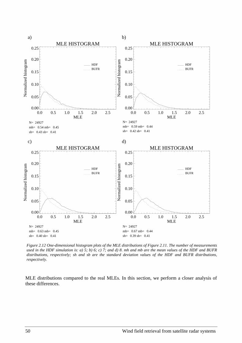
50 Wind field retrieval from satellite radar systems
MLE distributions compared to the real MLEs. In this section, we perform a closer analysis of these differences.
a) b) MLE HISTOGRAM
0.0 0.5 1.0 1.5 2.0 2.5MLE
0.00
0.05
0.10
0.15
0.20
0.25
Nor
mal
ized
his
togr
am
HDF
BUFR
N= 24927
mh= 0.54 mb= 0.45
sh= 0.43 sb= 0.41
MLE HISTOGRAM
0.0 0.5 1.0 1.5 2.0 2.5MLE
0.00
0.05
0.10
0.15
0.20
0.25
Nor
mal
ized
his
togr
am
HDF
BUFR
N= 24927mh= 0.59 mb= 0.44sh= 0.42 sb= 0.41
c) d)
MLE HISTOGRAM
0.0 0.5 1.0 1.5 2.0 2.5MLE
0.00
0.05
0.10
0.15
0.20
0.25
Nor
mal
ized
his
togr
am
HDF
BUFR
N= 24927mh= 0.63 mb= 0.45sh= 0.40 sb= 0.41
MLE HISTOGRAM
0.0 0.5 1.0 1.5 2.0 2.5MLE
0.00
0.05
0.10
0.15
0.20
0.25
Nor
mal
ized
his
togr
am
HDF
BUFR
N= 24927mh= 0.67 mb= 0.44sh= 0.39 sb= 0.41
Figure 2.12 One-dimensional histogram plots of the MLE distributions of Figure 2.11. The number of measurements used in the HDF simulation is: a) 5; b) 6; c) 7; and d) 8. mh and mb are the mean values of the HDF and BUFR distributions, respectively; sh and sb are the standard deviation values of the HDF and BUFR distributions, respectively.

Chapter 2. Maximum likelihood estimation 51
Distributions
Similar to Figure 2.12, Figure 2.13 shows the one-dimensional histograms of HDF and BUFR MLEs but for real (plot a) and simulated (realistic) (plot b) data. Note that the shape of the simulated HDF and BUFR distributions is different compared to the real distributions. In particular, the mean value of the BUFR distributions is larger for the simulated MLE than for the real MLE. Moreover, the SD value of the HDF distributions is substantially larger for the real compared with the simulated MLE. We also note that in the HDF real data there is a larger accumulation of values in the vicinity of zero MLE.
Mean values versus node number and wind speed
In order to better understand these differences in the MLE distributions, we study the behavior of the mean simulated and real MLE as a function of wind speed and cross-track location.
Figure 2.14 shows the mean MLE surface as a function of wind speed and node number for the HDF (plot a) and BUFR (plot b) real data (same surfaces as Figures 2.5b and B.2a, respectively, but for the 1st rank instead of the selected MLE). The noise in the MLE surfaces, caused by geophysical effects (such as rain) and/or small amount of data (at high winds), is filtered out (see section 2.3.1). The MLEs used in this Figure correspond to the MLEs of the 1st rank solutions provided in both QuikSCAT data products (HDF and BUFR). Figures 2.15a and 2.15b show the same surfaces as Figures 2.14a and 2.14b, respectively, but for simulated data. The MLEs used in this Figure correspond to the MLEs of the 1st rank solutions provided by the KNMI inversion software.
a) b) MLE HISTOGRAM
0.0 0.5 1.0 1.5 2.0 2.5MLE
0.00
0.05
0.10
0.15
0.20
0.25
Nor
mal
ized
his
togr
am
HDF
BUFR
N=1114381
mh= 0.57 mb= 0.28
sh= 0.53 sb= 0.40
MLE HISTOGRAM
0.0 0.5 1.0 1.5 2.0 2.5MLE
0.00
0.05
0.10
0.15
0.20
0.25N
orm
aliz
ed h
isto
gram
HDF
BUFR
N=1105137mh= 0.67 mb= 0.45sh= 0.40 sb= 0.42
Figure 2.13 One-dimensional histogram plots of the HDF and BUFR MLE distributions for real data (a) and the realistic simulation (b). The legend is the same as in Figure 2.12.

52 Wind field retrieval from satellite radar systems
a)
b)
Figure 2.14 Mean 1st-rank MLE versus wind speed and node number (only inner swath nodes are shown) for real data: (a) HDF and (b) BUFR. The speed binning is 1 m/s and the node binning is 1.
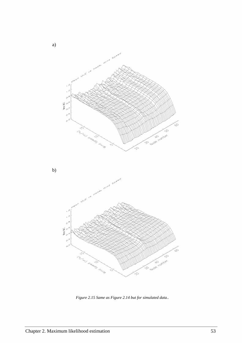
Chapter 2. Maximum likelihood estimation 53
a)
b)
Figure 2.15 Same as Figure 2.14 but for simulated data..

54 Wind field retrieval from satellite radar systems
In HDF, there is a slight increase of the surface with increasing distance to nadir (Figures 2.14a and 2.15a). The reason for this increase lies in the inversion. As the inversion is a non-linear process, the scaling (linear correction), that is, the Kp noise (see equation 2.9), is not sufficient to compensate for the increase in the MLE due to the increase in the number of σº. Nevertheless, the mean MLE surfaces show that this effect is minor. Note that the increase is stepwise in the simulated data (Figure 2.15a) and not monotonic as for real data (Figure 2.14a) because of the approximation in the number of σº made in the simulation of HDF data, that is, we use a constant number of measurements in each WVC while in reality the number of measurements per WVC varies (see Figure 2.9).
In BUFR, there is no increase in MLE with increasing distance to nadir (Figures 2.14b and 2.15b), as the number of σº is kept constant for all WVCs. As for the HDF case, the simulated MLE behaviour across track (Figure 2.15b) compares well with the real case in BUFR (Figure 2.14b).
If we compare the mean MLE behaviour as a function of wind speed between the real (Figure 2.14) and the simulated (Figure 2.15) cases, we see a large discrepancy at low speeds. In reality, the MLE increases with decreasing speed while in the simulated case the MLE decreases with decreasing speed.
The reason for this MLE increase in the real case is that the observation error (Kp) is underestimated for low wind speeds. From equation 2.9, an underestimation in the Kp (denominator term) will in turn produce an increase in the MLE. The Kp noise contains two terms: the instrument noise and the geophysical noise. Figa and Stoffelen (2000) provide a physically based model for the NSCAT backscatter observation error. They find that for low wind speed, the largest uncertainty lies in the spatial variability of the geophysical target (geophysical noise). Since the different view and polarization measurements in a WVC do not sample exactly the same area, the geophysical collocation error variability becomes substantial at low backscatter levels.
However, in the simulated case, the Kp is considered as a true value and therefore we would expect no increase or decrease in the MLE value at low wind speeds. This is however not the case. The problem lies in the inversion and, among others, in the fact that we assume that the measurement noise is proportional to the true value. The latter leads to a Kp that is proportional to σs° (simulated σ° from the GMF) in the denominator of equation 2.9. Stoffelen (1998a) explains on page III-29 how proportional errors cause positive bias in the solution (after inversion). This positive bias will in turn produce a decrease in the MLE. Figure 2.16 illustrates the problem in the case of a two-view measurement system (QuikSCAT has up to four views, but for simplicity we draw a 2D case). The solid curves represent the solution space. The diamond represents the pair of “true” measurements, which are the starting point in the simulation process. The solid circle around the diamond represents the “true” measurement noise (Kpt). Using this Kpt we simulate the measurement pair (triangle inside the solid circle). The dashed circle represents its corresponding estimated noise (Kpm). After inversion, we get a positively biased solution (star) which has its proportional noise (Kps) represented by the dotted circle. As Kps increases significantly, the MLE decreases (Kps is the denominator of equation 2.9) and this effect is more acute as we approach the origin corresponding to lower speeds.
Finally, it is clear that the mean MLE at mid and high speeds is significantly larger for simulated data than for real data (see the surface plateau level of Figure 2.15 compared to Figure 2.14). This means that there is an overestimation of the Kp (or measurement) noise at these speed regimes.

Chapter 2. Maximum likelihood estimation 55
Since the largest uncertainty at these speeds lies in the instrument noise and not in the geophysical noise, we conclude that there is probably an overestimation of the instrument noise.
Main differences
According to the analysis, we conclude that the remaining differences between the simulated and the real distributions can be attributed to the following:
• The simulation of the number of σº per WVC and view in HDF is just a rough approximation. In the real data a WVC can contain a variable number of σº (see Figure 2.9) and in the simulation we have fixed this number.
• The different behaviour of the real and simulated MLEs at low speeds as discussed above (see Figures 2.14 and 2.15). In the real data, the estimated Kp values, and more specifically the geophysical noise values, are underestimated.
• An overall overestimation in the real data of the estimated Kp values (except at low winds where the opposite occurs), more specifically, the instrument noise values. This is deduced from the higher mean MLE values of both HDF and BUFR simulated distributions (Figure 2.15) compared to the mean values of the real distributions (Figure 2.14).
Figure 2.16 Schematic illustration of the effect of proportional noise on MLE in a 2D measurement space.
σ° (view 1)
σ° (
view
2)

56 Wind field retrieval from satellite radar systems
There may be other reasons that could cause minor differences in the distributions, such as processing of eggs or composites, i.e., for real data HDF uses eggs and BUFR composites (see Appendix A), whereas for simulated data we treated both HDF and BUFR as composites. Nevertheless and as discussed in the previous section, these differences are not so relevant as the simulation is a good reflection of reality.
2.4.4 MLE influence on wind retrieval
In the previous sections, we have shown how different the MLE distributions are in HDF and BUFR. In the BUFR product, σ° measurements are combined to result in only 4 independent σ°s. In HDF, on average, 8 σ° measurements are available per WVC in the sweet swath. This data reduction could cause information in the σ° measurements to be lost. As such, the poor BUFR and HDF MLE comparison should be taken seriously. In this section, we investigate in some detail the wind retrieval performance properties of SeaWinds BUFR as compared to HDF. For such purpose, we perform triple collocations of HDF, BUFR and ECMWF winds.
Figure 2.17 shows the two-dimensional histograms of BUFR winds versus HDF winds (upper plots), BUFR versus ECMWF (middle plots) and HDF versus ECMWF (bottom plots). The left plots correspond to the histograms of wind speeds and the right plots to the histograms of wind directions. Both BUFR and HDF retrieved winds correspond to the 1st rank solution.
From the upper plots we note that the BUFR and HDF retrieved winds are not identical, although very similar. Figure 2.17a shows almost no bias in speed and a very small SD (0.58 m/s). Figure 2.17b shows a typical effect of comparing 1st rank solutions, which is the secondary distribution around 180°. This is due to the fact that 1st and 2nd rank solutions (often with very similar wind speed but wind direction 180° apart) can have very similar MLE values and therefore be switched from one data product to the other. This effect leads to very high directional SD values. Still, we can see from the correlation factor (0.87) that the retrieved directions are similar.
Looking at the middle and bottom plots of Figure 2.17, we can see almost no difference between HDF and BUFR when compared to ECMWF winds. Figures 2.17c and 2.17e show almost identical wind speed distributions with almost the same bias and SD. Figures 2.17d and 2.17f show very similar wind direction distributions with almost the same correlation factor.
Therefore, we conclude that the difference in the MLE distributions is not affecting the quality of the retrieved winds. Moreover, as we will see in chapter 5, the QC skills in BUFR and HDF are also similar.

Chapter 2. Maximum likelihood estimation 57
a) b) WINDS HISTOGRAM
5 10 15 20Wind speed (m/s) - HDF
5
10
15
20
Win
d sp
eed
(m/s
) -
BU
FR
N=1114381
mx= 7.87 my= 7.89
m(y-x)= 0.02 s(y-x)= 0.58
cor_xy= 0.99
WINDS HISTOGRAM
0 90 180 270 360Wind dir (deg) - HDF
0
90
180
270
360
Win
d di
r (d
eg)
- B
UF
R
N= 962552
mx= 196.92 my= 196.76
m(y-x)= -0.16 s(y-x)= 51.54
cor_xy= 0.87
c) d) WINDS HISTOGRAM
5 10 15 20Wind speed (m/s) - ECMWF
5
10
15
20
Win
d sp
eed
(m/s
) - B
UFR
N=1060810
mx= 7.59 my= 7.85
m(y-x)= 0.26 s(y-x)= 1.90
cor_xy= 0.86
WINDS HISTOGRAM
0 90 180 270 360Wind dir (deg) - ECMWF
0
90
180
270
360W
ind
dir (
deg)
- B
UFR
N= 856586
mx= 196.51 my= 197.07
m(y-x)= 0.56 s(y-x)= 57.30
cor_xy= 0.85
e) f) WINDS HISTOGRAM
5 10 15 20Wind speed (m/s) - ECMWF
5
10
15
20
Win
d sp
eed
(m/s
) - H
DF
N=1058882
mx= 7.60 my= 7.85
m(y-x)= 0.25 s(y-x)= 1.89
cor_xy= 0.86
WINDS HISTOGRAM
0 90 180 270 360Wind dir (deg) - ECMWF
0
90
180
270
360
Win
d di
r (de
g) -
HD
F
N= 858657
mx= 197.22 my= 197.87
m(y-x)= 0.65 s(y-x)= 58.67
cor_xy= 0.84
Figure 2.17 Two-dimensional histogram of BUFR winds versus HDF winds (top plots), BUFR winds versus ECMWF winds (middle plots) and HDF winds versus ECMWF winds (bottom plots). The left plots correspond to wind speeds (bins of 0.4 m/s) and the right plots to wind directions (bins of 2.5°). Only ECMWF winds above 4 m/s are used in the wind direction plots. The legend and contour lines are the same as in Figure 2.2.

58 Wind field retrieval from satellite radar systems
2.5 Conclusions
The MLE is an optimization technique derived from a Bayesian approach, which is generally used in meteorological analysis. This technique, as applied in scatterometry, maximizes the probability of being the “true” wind by minimizing a cost function, which uses no prior or background information.
In scatterometry, the standard wind retrieval procedure works as follows: the minima of the MLE cost function, considered as the ambiguous wind solutions, are in turn used by the AR procedure to select the observed wind. In these circumstances, it is shown how the shape of the MLE cost function determines the skill of the wind retrieval procedure in terms of ambiguity and accuracy. In particular, for QuikSCAT, the shape gradually changes with the cross-track location (WVC), thus affecting the retrieval skill of the different swath regions. On the one hand, in the regions with only two views, i.e., outer regions, where the cost function minima are usually equally deep, there is an important ambiguity problem. On the other hand, in the regions with poor azimuth diversity such as the nadir region or the edges of the outer swath, where the cost function minima are broad, the accuracy of the retrieved winds is substantially lower compared to the rest of the swath. The cost function shape is therefore reflecting the limitations of the inversion. As such, a new wind retrieval procedure, which appropriately takes into account these limitations, would improve the wind retrieval skill, in comparison with the standard procedure.
The MLE usually presents some unwanted dependencies to certain parameters, such as the node number or the wind condition. In order to remove these dependencies, the MLE is normalized (Rn). The dependencies are mainly caused by miscalculations of the measurement noise. Therefore, accurate information on the measurement noise is needed in the normalization factor (<MLE>). In the absence of a noise model, a good noise indicator is the mean behavior of the MLE. A method, which uses the mean MLE information to empirically derive the <MLE> for QuikSCAT, is presented. It is shown that the wind direction dependencies of the mean MLE are not real but rather due to some deficiencies in the inversion. The <MLE> is consequently computed from the mean MLE dependencies on the node number and retrieved wind speed. The Rn represents a more stable parameter, compared to the MLE, and is very useful for wind retrieval and QC purposes. This empirical method, although applied for QuikSCAT in here, is generic and, as such, can be used to determine the Rn of any scatterometer system.
A comparison between the MLE of two different data formats, the QuikSCAT HDF and BUFR products, shows that both MLE distributions are poorly correlated. A comprehensive characterization of the MLE is performed in order to fully understand the MLE distribution differences. A very simple example is solved theoretically to show that the different level of averaging of the data in HDF and BUFR (i.e., the BUFR σ° is an average of the HDF σ°s per view) can be the main cause. From simulated MLE distributions with different number of measurements (BUFR and HDF), we conclude that the small correlation of the MLE distributions of both formats is due to the σ° averaging. The simulation results validate the assumptions used in the theoretical case.
Further simulations show how the MLE distributions change as a function of the number of observations taken. The higher the difference in the number of HDF and BUFR observations, the smaller the correlation and the higher the mean MLE value difference between the two products.

Chapter 2. Maximum likelihood estimation 59
The remaining differences between simulated and real MLEs are also analysed in detail. Misestimation of the real measurement noise and simplification in the computation of the number of measurements for both formats in the simulation are pointed out as the main cause for these differences.
Despite the small correlation between the HDF and the BUFR MLEs, the wind retrieval of both formats is of comparable quality. As one might expect, the QC properties in BUFR and HDF show no major differences as well (see section 5.1.5). Therefore, we conclude that the information content of the product is not significantly affected by the σ° averaging.

60 Wind field retrieval from satellite radar systems

Chapter 3. Wind retrieval for determined problems: QuikSCAT case 61
Chapter 3
Wind Retrieval for Determined Problems:
QuikSCAT Case
Scatterometers provide σ° measurements from multiple views and as such generally wind speed and direction can be determined. However, the level of determination of the problem depends very much on the number and relative geometry of radar views. This is well illustrated in section 1.4.1 with several cases. The radar instrument that represents all these cases, especially the determined ones (cases b-d of section 1.4.1), is QuikSCAT (see section 1.4.3). Therefore, in order to study the wind retrieval for determined problems, it seems reasonable to focus on such instrument.
In chapter 2, the wind retrieval skill in the different parts of the QuikSCAT swath is extensively discussed. Although the geometry varies with the node number, the good azimuth diversity of the sweet regions is comparable to that of other scatterometer systems, such as NSCAT or ERS SCAT, leading to accurate winds. In the outer regions however, there is a significant ambiguity problem but, as discussed in section 2.2.2, the accuracy is comparable to that of the sweet swath. Therefore, if there is a way to remove the inherent ambiguity, the outer swath could provide accurate winds. This is feasible when using a consistent AR scheme, as shown by Stoffelen and Cats (1991) for the Seasat SASS (comparable geometry to the QuikSCAT outer swath). The wind retrieval over the poor-azimuth-diversity nadir region is inaccurate and has no precedent in scatterometry; as such, special attention should be given to it.
In this chapter, the standard wind retrieval procedure used in scatterometry will be described and implemented for QuikSCAT use. An alternative method will be proposed in order to improve wind retrieval, notably in the nadir region. Both procedures will then be validated and inter-compared with the help of independent NWP wind information.
As inferred from Figure 1.9 (section 1.4.3), the QuikSCAT azimuth diversity smoothly changes with the node number in the inner swath. In other words, there is no discontinuity between the sweet and the nadir regions. As such, it seems reasonable to consider the sweet swath as well for this study. Therefore, we focus our research on improving wind retrieval in the inner swath (sweet + nadir), giving special attention to the nadir region. However, this does not mean that the methodology applied for the inner swath is not valid for the outer swath. Moreover, as will be

62 Wind field retrieval from satellite radar systems
further discussed in section 6.1.2, the results from this chapter are applicable to the outer swath as well.
3.1 Standard procedure
The scatterometer wind retrieval procedure consists of inversion, QC, and AR. In this section, we describe the standard inversion + AR methodology used in scatterometry. Regarding the QC procedure, there is no standard procedure (up to now); different methods have been used in the past for the different instruments. Because of its importance and independence from the retrieval procedure used, a separate chapter is dedicated to QC (see chapter 5).
3.1.1 Inversion
The MLE-based inversion has already been exhaustively discussed in chapter 2. The standard procedure gives up to four ambiguous wind solutions, corresponding to the cost function minima. In the process of deriving such minima, several parameters can be tuned to improve the inversion in terms of ambiguity and quality. An example on how to perform a comprehensive inversion tuning, in this case, for QuikSCAT is shown in Appendix C. The tuning, although improving the overall wind retrieval skill, does not solve any of the already discussed inherent inversion problems, as seen from the significantly lower skill of the nadir region, compared to the sweet regions (see Appendix C).
As an interface between the inversion and the AR, a natural step in scatterometry is to convert the MLE into a solution probability. As can be inferred from the equations of section 2.1, the probability of being the “true” wind given a set of scatterometer observations is related by definition to the MLE in the following way:
2/1)|( MLEo e
kvp −=σ , (3.1)
where v represents the “true” wind and σ° the set of backscatter measurements, and k is a normalization factor. The theoretical relationship is therefore an exponential. In other words, as the MLE, which represents the misfit of the measurements with the solution lying on the GMF surface, increases, the probability of that particular solution being the “true” wind decreases exponentially. In reality, for several reasons such as the miscalculation of the measurement noise (see section 2.3), the shape of the exponential may differ from the theory. A comprehensive characterization of the solution probability for QuikSCAT, based on the empirical methodology described by Stoffelen et al. (2000), follows.

Chapter 3. Wind retrieval for determined problems: QuikSCAT case 63
Empirical solution probability
• We use the Rn instead of the MLE to avoid the already mentioned problem in the measurement noise estimation, such that equation 3.1 is re-written as:
lRno ek
vp /
'
1)|( −=σ (3.2)
where k’ is again a normalization factor, and l is the parameter that we want to empirically derive. Since we are not using the JPL inversion but the KNMI “tuned” inversion (i.e., NSCAT-2 GMF, no smoothing and 3D interpolation, as discussed in Appendix C), the <MLE>, used to calculate the Rn (see equation 2.10), is re-computed (see Appendix B.3).
• In order to empirically derive equation 3.2, we can ignore the a priori knowledge on the exponential behavior of the probability, and make the following assumption: There exists a function ps(x) such that, if we have a set of inversion solutions vi with normalized residual Rni, then the probability that rank j is the one closest to the true wind, denoted by s=j, is given by
∑=
=∈= N
iis
jsi
Rnp
RnpNiRnjsP
1
)(
)(}),1{,|( (3.3)
• To determine ps(x), we concentrate first on only those cases which have exactly two solutions. We process about 2.5 days of QuikSCAT BUFR data and we collocate them with ECMWF winds. The closest solution to the ECMWF wind is used as the “selected” wind. Therefore, we can construct a two-dimensional histogram showing the relative probability of selecting the 1st rank (or the 2nd rank), as a function of Rn1 and Rn2. But according to our assumption, by applying equation 3.3 with N=2, we find that the probability of selecting the 1st rank is given by
112
21
121 )}(/)(1{
)()(
)(),|1( −+=
+== RnpRnp
RnpRnp
RnpRnRnsP ss
ss
s (3.4)
• Therefore, by re-arranging equation 3.4, the two-dimensional histogram gives an estimate of ps(Rn2)/ ps(Rn1) for every combination of Rn2 and Rn1. Figure 3.1a shows such experimentally determined ratios as a function of Rn2 - Rn1, for several values of Rn1. Although for Rn1 = 2.5 the ratio is somewhat noisy, it is discernible that the ratio is a fairly invariant function of Rn2 - Rn1. Since Rn1 is constant and therefore ps(Rn1) is also a constant, this plot is actually showing the shape of ps(x).
• As we know from equation 3.2, the shape of ps(x) is exponential and therefore we just have to fit the exponential to the experimental function of Figure 3.1a by adjusting the l parameter. Figure 3.1b shows the best fit to Figure 3.1a, which is represented by the following function:
4.1/)( xs exp −= (3.5)

64 Wind field retrieval from satellite radar systems
where x is representing the Rn.
In order to check whether the assumption is correct and the ps(x) we found can be generalized for any number of solutions and not only for two, we use the probability function to predict how often a certain solution rank corresponds to the “true” solution for a varying number of solutions and varying distributions of Rni (remember that we have used only a few constant Rn1 values to fit the distributions of Figure 3.1a). Tables 3.1 and 3.2 compare the predicted distributions over the different ranks (same stratification as tables in Appendix C) with the “observed” distributions (using the closest to ECMWF) in the sweet and the nadir swaths respectively, for the set of about 2.5 days of collocated QuikSCAT-ECMWF data. As shown, when comparing the left side to the right side of the columns, the correspondence is remarkable1. Therefore, we conclude that the assumption is correct and that equation 3.5 can be used to determine the solution probability.
1 Note that the right side of the columns of tables 3.1 and 3.2 compare well as expected with the columns of tables C.1 and C.2 respectively, since the only difference is the data set used, i.e., much larger in the latter tables.
a) b)
Figure 3.1 Plot a shows the ratio of the number of realizations of Rn2 and the number of realizations of Rn1 as a function of Rn2 – Rn1, and for values of Rn1=0.1 (solid), Rn1=1.1 (dashed), and Rn1=2.5 (dotted). Plot b shows the single exponential fit to the curves of plot a

Chapter 3. Wind retrieval for determined problems: QuikSCAT case 65
Table 3.1 Predicted / observed distributions at 25-km (sweet swath)1. 2 Solutions 3 Solutions 4 Solutions All Solutions
Number of Data 331666 233477 317373 882516
Rank 1 91 / 90 82 / 82 77 / 79 84 / 84
Rank 2 9 / 10 15 / 15 18 / 17 14 / 14
Rank 3 - 3 / 3 4 / 3 2 / 2
Rank 4 - - 1 / 1 0 / 0
Table 3.2 Predicted / observed distributions at 25-km (nadir swath)1. 2 Solutions 3 Solutions 4 Solutions All Solutions
Number of Data 262753 172506 45638 480897
Rank 1 82 / 80 79 / 79 65 / 66 79 / 79
Rank 2 18 / 20 17 / 17 20 / 19 18 / 18
Rank 3 - 4 / 4 8 / 8 2 / 2
Rank 4 - - 7 / 7 1 / 1
1 Non-smoothing and 3D interpolation have been used in the inversion.
3.1.2 Ambiguity removal
In order to understand the importance of the solution probability for AR, a brief description of AR follows. As discussed in section 1.4, the AR is the process of selecting a unique wind vector out of a set of ambiguous wind vectors at each WVC. The AR is not computed in a WVC-by-WVC basis but over many neighbouring WVCs at once. There are two AR techniques, which are commonly used in scatterometry: spatial filters, e.g., median filter for QuikSCAT, and variational analysis.
Median filter
The median of a group of data values is that value for which there are equal numbers of data values of greater and lesser magnitude. This conventional definition of the median can only be applied to non-circular (i.e., linear and scalar) data in which the ordering of the values is obvious. For circular data or vector data such as scatterometer winds, an alternative definition of median is

66 Wind field retrieval from satellite radar systems
used. The median of a set of data x(1), x(2),…,x(N) is defined as the number x(M) which minimizes:
∑=
−N
i
ixMx1
)()( (3.6)
where NM ≤≤1 .
The medians of circular and vector data calculated using the alternative definition have similar characteristics to the median of non-circular data, i.e., extreme and isolated data are ignored.
The median filter is used by JPL for QuikSCAT AR (JPL, 2001) and works as follows:
• The wind field over an entire revolution of scatterometer data is initialised with the help of an NWP model. For each particular WVC, the 1st rank or the 2nd rank wind vector solution, whichever is closer to the NWP field, is selected as first guess wind. The number of ranked solutions used for initialisation does not necessarily need to be two (see section 3.2).
• The wind vectors in a 7 x 7 filter window determine a median vector for the center WVC. The median vector is compared with the ambiguities in that WVC, and the closest ambiguity to the median is selected for use in the next iteration. The entire revolution is filtered in that way. The process continues until it converges, i.e., when no new replacements of vectors have been made.
The MLE (or probability) information is implicitly used in the median filter. The probability can play an important roll in the selection of ambiguities used in the initialization and filtering processes (this is further discussed in section 3.2). However, it is never used explicitly in this AR technique.
Variational analysis
The variational analysis is a commonly used technique for data assimilation into NWP models. It consists of combining the background field (NWP) with the observations, assuming that both sources of information contain errors and these are well characterized, to get an analysis field, which is spatially consistent and meteorologically balanced. This analysis field can then be used for scatterometer AR, that is, to select the closest ambiguous wind solution to the analysis field at each WVC. At KNMI, a simple 2D (at surface level only) variational analysis scheme (2D-Var) has been specifically developed for AR (Stoffelen et al., 2000), which attempts to minimize the cost function
scatob JJxJ +=)(δ , (3.7)
where Jb is the background term and Joscat is the observation term. It uses an incremental
formulation with the control variable of wind increments, bxxx −=δ , defined on a rectangular
equidistant grid. The control variable xb is the background field, which in 2D-Var is a NWP model forecast. The forecast is also used as first guess making the control variable equal to the null-vector at the start of the minimization.

Chapter 3. Wind retrieval for determined problems: QuikSCAT case 67
The Jb is a quadratic term that contains the inverse of the background error covariance matrix. It penalizes the deviation from the background field. The Jo
scat expresses the misfit between the ambiguous wind vector solutions and the control variable at each observation point. The contribution of the wind solutions in each observation point is weighted by the solution probability.
In order to solve the minimization problem, a conjugate gradients method is used, which also requires the gradient of the cost function. After convergence, the control variable vector of wind increments is added to the background field to obtain the wind analysis. The analyzed wind field is then used for AR, as already discussed.
The solution probability is indeed used explicitly in this AR technique. It plays a very important roll in the minimization and therefore must be characterized in a comprehensive way. In this respect, the empirically derived solution probability, shown in the previous section, is essential for a successful use of a variational analysis AR.
3.1.3 Relevance of spatial resolution
KNMI has a NRT 100-km resolution QuikSCAT wind product, which includes inversion, QC and ambiguity removal. Stoffelen et al. (2000) show that the 25-km QuikSCAT winds are often too noisy, especially at low winds and in the nadir region. They also show that the averaging of the radar backscatter information, and therefore the reduction of the spatial resolution, significantly reduces the noise of the inverted winds and the rank-1 probability (see also Portabella et al., 2001). For applications such as mesoscale NWP data assimilation, where the effective resolution of the models is never lower than 100-200 km, the use of reduced resolution QuikSCAT winds is very promising. In this respect, ECMWF is now using a reduced resolution QuikSCAT wind processing for assimilation purposes. Therefore, a comparison between the 25-km and the 100-km inversions seems appropriate at this stage, and can in turn help to better understand the QuikSCAT inversion problem.
Probability at 100-km
We can perform this comparison in terms of the probability, since it is a closer stage to AR (see section 3.1.1) than the MLE. Therefore, we first compute the probability for the 100-km product, following the same methodology as for the 25-km product (see section 3.1.1):
• In order to get a Rn at 100-km resolution, the corresponding <MLE> (see equation 2.10) is computed (see Appendix B.4).
• The shape of ps(x) is found by processing about 10 days of QuikSCAT data and shown in Figure 3.2 for the same values of Rn1 as used in Figure 3.1a. The curves are noisier than in Figure 3.1a, since the number of data used in the 100-km two-dimensional histogram is about four times smaller than that used in the 25-km histogram (one 100-km WVC corresponds to sixteen 25-km WVCs). Despite this noise, note that the curve of Figure 3.1b fit also fairly

68 Wind field retrieval from satellite radar systems
well the curves of Figure 3.2. Therefore, we also use equation 3.5 to compute the solution probability at 100-km, where x is in this case the Rn at 100-km resolution.
• Similar to tables 3.1 and 3.2, the results for the verification of the 100-km probability are shown in tables 3.3 and 3.4 respectively. The correspondence between the predicted and the observed distributions is also remarkable, confirming the validity of equation 3.5 for computing 100-km probability.
Comparison
By comparing tables 3.1 and 3.2 to tables 3.3 and 3.4 respectively, one can clearly see the substantially higher 1st rank skill of the 100-km product, denoting a smaller ambiguity problem (see section 2.2.2 and Appendix C), compared to the 25-km product (note the higher percentages of the rank-1 row in the 100-km tables in comparison with the 25-km tables).
In order to compare both products, we have transformed the MLE cost function into a probability cost function by using equation 3.5. We invert the already mentioned sets of BUFR data (2.5 days for the 25-km and 10 days for the 100-km) and keep the probability cost function information. [Note that discussing about peaks or maxima in the probability cost function is equivalent to the discussion about minima in the MLE cost function]. Figure 3.3 shows the statistical results of looking at several characteristics of the cost function.
Figure 3.2 Same as Figure 3.1a but for the 100-km resolution Rn

Chapter 3. Wind retrieval for determined problems: QuikSCAT case 69
Table 3.3 Predicted / observed distributions at 100-km (sweet swath)1.
2 Solutions 3 Solutions 4 Solutions All Solutions
Number of Data 53753 67947 73269 194969
Rank 1 97 / 96 94 / 93 92 / 92 94 / 93
Rank 2 3 / 4 5 / 5 7 / 7 5 / 6
Rank 3 - 1 / 2 1 / 1 1 / 1
Rank 4 - - 0 / 0 0 / 0
Table 3.4 Predicted / observed distributions at 100-km (nadir swath)1.
2 Solutions 3 Solutions 4 Solutions All Solutions
Number of Data 66618 40478 9344 116440
Rank 1 83 / 83 93 / 93 78 / 74 86 / 86
Rank 2 17 / 17 6 / 6 16 / 19 13 / 13
Rank 3 - 1 / 1 3 / 4 1 / 1
Rank 4 - - 3 / 3 0 / 0
1 Non-smoothing and 3D interpolation have been used in the inversion.
The top plots of Figure 3.3 show the histograms of the difference between the maximum (Pmax) and the minimum (Pmin) probabilities for the 25-km (plot a) and the 100-km (plot b) products. The distributions of Figure 3.3b are much broader and shifted towards higher probability difference values than the distributions of Figure 3.3a, denoting a better probability modulation and therefore accuracy (see section 2.2.1) of the 100-km product. Comparing the sweet (solid lines) with the nadir (dotted lines), we see a better probability modulation for the former in both products.
The middle plots of Figure 3.3 show the histograms of the number of cost function points with probability larger than 10% for the 25-km (plot c) and the 100-km (plot d) products. As discussed in section 2.2, the cost function is computed at the direction step size of the GMF LUT (2.5°) and therefore contains 144 points. The fact of having at least one point above 10% probability is an indication of a good probability modulation since it shows how likely these points are with
respect to the remaining cost function points with average likelihood of =144
1 0.7%. In this
sense, notice the larger amount of times that the 25-km product cost function does not have any probability value above 10% compared to the 100-km product, showing again a better probability modulation of the latter. In a similar way, if we compare the sweet with the nadir swaths, we notice a larger number of times (the double or more) where no cost function points were above

70 Wind field retrieval from satellite radar systems
a) b)
c) d)
e) f)
Figure 3.3 Histograms of the difference between the maximum (Pmax) and the minimum (Pmin) probabilities (top plots), the number of cost function points with probability larger than 10% (middle plots), and the difference between Pmax and the mean probability (Pmean) over an interval of ±12.5° around Pmax (bottom plots), for the sweet (solid lines) and the nadir (dotted lines) regions and for the 25-km (left plots) and the 100-km (right plots) products.

Chapter 3. Wind retrieval for determined problems: QuikSCAT case 71
10% probability in the latter. However, the fact of having more or less points above 10% does not necessarily show a better modulation. For example, if we look at the shape of the distributions in Figure 3.3d, we see that the nadir swath distribution is shifted towards a larger number of points compared to the sweet swath. Since the nadir swath does not usually have more than 3 solutions (look at the number of data with 4 solutions in comparison with the number of data with 2 or 3 solutions in table 3.4), the relatively large number of points above 10% probability could be an indication of a flat peak, as expected from this region of the swath (see section 2.2.2).
The bottom plots of Figure 3.3 show the histograms of the difference between Pmax and the mean probability (Pmean) over an interval of ±12.5° around Pmax for the 25-km (plot e) and the 100-km (plot f) products. This difference gives an indication of the peak modulation. The larger the difference, the steeper the maximum (or main peak) of the cost function and therefore the better the accuracy of retrieved winds is (see sections 2.2.1 and 2.2.2). The larger accumulations of data at low difference values in the nadir swath (dotted) with respect to the sweet (solid) swath confirms the existence of flatter peaks in the former as discussed above. Moreover, this is not only valid for the 100-km product but also for the 25-km product. The reason why we could not infer flat peaks in the 25-km product from the middle plot distributions is that the flat peaks are below the 10% probability level imposed in such plots. However, as we see from the larger accumulation of data at low Pmax-Pmean values in Figure 3.3e with respect to Figure 3.3f, the peaks are much flatter (lower peak modulation) at 25-km than at 100-km resolution.
Therefore, we conclude that, for QuikSCAT, the 100-km product is less ambiguous and more accurate than the 25-km product and therefore more suitable for wind retrieval purposes than the 25-km product. In this chapter, we will therefore use the 100-km product.
3.2 Multiple solution scheme
So far, we have extensively examined the inversion problem for QuikSCAT, tuned the inversion in order to reduce its ambiguity and improve its accuracy, and determined the relation between the relative probability of a solution and the MLE in order to prepare QuikSCAT ambiguous solutions for AR. We have learned that in the nadir swath, the accuracy of the inverted winds is low compared to the sweet swath, due to low peak modulation in the probability cost function. For low winds, the accuracy is also low due to the low cost function modulation. The worst scenario therefore occurs for low winds in the nadir swath, where the cost function modulation is rather flat.
The number of solutions in the nadir swath is smaller than in the sweet swath (see the relatively small amount of data with 3 and 4 solutions compared with 2 solutions in table 3.4, in contrast with table 3.3). This may be caused by the noise and/or the shape of the cost function, i.e., a cost function that has well defined and steep probability peaks (or MLE minima) may have a larger number of peaks than a cost function that has broad peaks. However, it seems contradictory to provide less wind solutions to AR when the cost function peaks are less well defined, since for such cases the information content of the wind solutions is poor. Along a broad peak, there are several wind solutions with almost the same relative probability as the peak. However, by selecting only one (as the inversion is doing), we assign zero probability to the rest of the points that belong to the broad peak. On the other hand, by selecting all of the points of the broad peak, we are transferring to AR all retrieved information; that is, the inversion could not find a clear
72 Wind field retrieval from satellite radar systems
candidate for that particular region of the cost function, but rather a few candidates with comparable probability.
Precedent
At JPL a procedure, based on a multiple solution inversion output (not constrained to four solutions) in combination with AR, called DIRTH (Stiles et al., 2000) was developed. It includes an initialization technique for the median filter, called the Thresholded Nudging (TN), and a multiple solution selection scheme as input to the median filter, called the Direction Interval Retrieval (DIR).
The TN allows for more than two ambiguities in the initialization (see section 3.1.2) and works as follows. The probability1 of the cost function is normalized with the probability of rank 1, and the number of ambiguities (up to four) with normalized probability above 0.2 is used in the initialization.
The DIR performs AR in the following way. Given a threshold T (0.8), a set of cost function points around each of the local maxima (resulting in as many segments as local maxima) is selected such that the number of points is minimized and the integral of the cost function over the interval of such points is T. Then, AR is performed in the usual manner (except for using the TN for initialization), and only the segment of points around the selected ambiguity is further used by the median filter (see section 3.1.2).
By examining many wind field cases, we conclude that the DIRTH winds are often very smooth and unrealistic in the nadir swath. Here we identify some possible reasons for this result:
• By applying the median filter only on the segment that was selected in the first place by the “traditional” AR, the scheme is subject to the accuracy of the latter. That is, if the traditional AR fails in an area and produces the wrong solutions, all the segments used in that area will in turn produce a more or less smooth field (probably following some segment extremes, depending on the segment width) but wrong.
• When using a threshold T of 0.8 to define the segments, it may well happen that the remaining cost function points that sum a probability of 0.2 (1-T) contain valuable information indeed. In particular, if we look at the Pmax - Pmin distributions in the nadir swath for 25-km resolution (Figure 3.3a), we see a relatively poor probability modulation. In such region, many cost function points with substantial probability may be left out of the segment selection. This will in turn decrease the quality of the wind retrieval.
The reason for setting such threshold T is to prevent oversmoothing. That is, if we use T=1, all data in the cost function will be used by the median filter, which in turn will result in a wind field inhibited by the NWP reference and the median filter characteristics. This is due to a very important limitation of the median filter AR, which is not explicitly using the relative probability of each solution, but rather considering all the solutions with identical probability. Despite the mentioned threshold and as already discussed, the resulting wind field is still substantially smooth in areas with large solution segments, i.e., the nadir region. Since the median filter does not
1 Stiles et al. (2000) use the theoretical relation between MLE and probability, i.e., equation 3.1, to compute the latter.

Chapter 3. Wind retrieval for determined problems: QuikSCAT case 73
ensure meteorologically balanced fields, the retrieved winds are not only oversmoothed but also unrealistic in some (of such) areas.
Alternative
The 2D-Var AR (see section 3.1.2) explicitly uses the probability of all ambiguous solutions. This AR therefore allows the possibility of using as many ambiguous solutions as we desire without a substantial risk of oversmoothing. Moreover, since the variational analysis is always constrained to spatial consistency and meteorological balance, we can ensure realistic retrieved winds by using a scheme based on a multiple solution inversion output in combination with such AR.
Figure 3.4 shows a QuikSCAT retrieved wind field, using the standard inversion output (up to four ambiguous wind solutions) and the 2D-Var AR. In the nadir region, it is clearly discernible that the retrieved wind field is spatially inconsistent. Since the 2D-Var analysis field (not shown) is spatially consistent, the problem is most likely in the ambiguous solution distribution.
Figure 3.4 QuikSCAT retrieved wind field using the standard inversion output (cost function minima) and the 2D-Var AR. The acquisition date is January 15 2002 at 16 hours UTC. The solid lines separate the sweet-left (left side), the nadir (middle), and the sweet-right (right side) regions of the QuikSCAT swath.

74 Wind field retrieval from satellite radar systems
a)
b)
Figure 3.5 Same as Figure 3.4 but for QuikSCAT ambiguous wind field using (a) the standard inversion output (cost function minima); and (b) the multiple solution scheme. Only solutions with probability above 10-5 (a) and 2x10⁻⁷ (b) are shown.

Chapter 3. Wind retrieval for determined problems: QuikSCAT case 75
Figure 3.5a shows the standard ambiguous solution distribution (MLE cost function minima) for the same case of Figure 3.4. As we can clearly see in the nadir region, the wind solution pattern shows almost no solutions in the direction of the mean flow. Therefore, even if the 2D-Var analysis field were of acceptable quality, there is no way to select a consistent wind field from such solution pattern.
Figure 3.5b shows the multiple ambiguous solution (not constrained to four) distribution again for the same meteorological case as Figures 3.4 and 3.5a. We show all the cost function solutions with probability above a guessed threshold1 of 2x10⁻⁷. Notice how often the ambiguous solutions in the sweet swath are around the cost function minimum, which is in the direction of the mean flow, denoting little ambiguity (main cost function minimum much deeper than the remaining minima) in comparison to the nadir swath. Note also that the number of solutions in the nadir region is large, indicating lower accuracy (broader minima) than in the sweet swath. In comparison with Figure 3.5a, we are providing much more information content to the AR using the multiple solution inversion output. As already discussed, the 2D-Var will use the information in an appropriate way (the ambiguous solutions are weighted by their computed probability) and therefore, from a theoretical point of view, the multiple solution concept should considerably improve the resulting analysis field. Moreover, the AR will now result in a spatially consistent wind field since the multiple solution concept does provide solutions aligned with the mean flow (see solution distribution in the nadir swath of Figure 3.5b). [Note: the dots in Figures 3.4 and 3.5 represent quality-controlled points. This issue is discussed in section 6.2.2.]
Therefore, it seems reasonable to test the multiple solution scheme (MSS) against the standard procedure. Since using all the points of the cost function with non-zero probability (up to 144) as solution ambiguities for the 2D-Var AR is computationally expensive, we use the mentioned probability thresholds, i.e., 10-5 for the standard procedure and 2x10⁻⁷ for the MSS, as a first guess.
3.3 Comparison between the standard procedure and the MSS
As discussed in section 3.1.2, the 2D-Var background term is a NWP forecast field. The QuikSCAT data products distributed by JPL and NOAA include collocated NCEP wind information. The latter is used for AR purposes, i.e., background term. As such, a different reference should be used to compare the standard wind retrieval and the MSS procedures. In this section, we use ECMWF winds as reference.
3.3.1 Statistical results
Three days of QuikSCAT and ECMWF collocated winds at 100-km resolution are used in the comparison. Table 3.5 shows the mean RMS of wind vector differences between ECMWF and three different wind sources: standard wind retrieval, MSS and NCEP. Comparing the standard procedure and the MSS, the latter shows better performance, i.e., agreement with ECMWF. As
1 The reason for choosing a different probability threshold in the standard procedure and the MSS is due to the normalization of the probability; the former is normalized with up to 4 solutions and the latter with up to 144.

76 Wind field retrieval from satellite radar systems
expected, the major difference between the two procedures is in the nadir region, where the RMS difference is more than 0.5 m/s lower for the MSS. In the sweet swath, the MSS also works better. This is due in part to an improvement at low winds, where low cost function modulation is expected, and in part to the improvement of the analysis field, i.e., a better 2D-Var analysis in nadir is expected to positively impact the analysis in the sweet regions. Indeed, the results (not shown) indicate better agreement of MSS analysis (compared to standard analysis) with ECMWF in both the sweet and the nadir swath.
Table 3.5 Mean vector RMS1 (m/s)
Swath region
Standard procedure
MSS NCEP
Sweet 2.48 2.23 2.85
Nadir 2.98 2.45 2.96 1 The vector RMS is referred to as the RMS of the wind vector difference between ECMWF and the different wind sources shown in the table.
Both the standard procedure and the MSS show generally better scores (against ECMWF) than NCEP (see table 3.5). This suggests that 2D-Var is successfully exploiting the observations rather than to follow the background (i.e., NCEP). As such, the quality of the background does not significantly affect the quality of the retrieved winds. This is also true in the nadir region. As discussed in section 3.2, the MSS provides a larger number of equally likely ambiguous solutions in the nadir swath, compared to the sweet regions, thus resulting in a larger influence of the background term in 2D-Var. However, the impact of NCEP in the nadir is also minor, as seen from the substantial difference in vector RMS between the MSS (2.45 m/s) and NCEP (2.96 m/s). The observations and the constraints on meteorological balance and spatial consistency are therefore the most dominant factors in the retrieval.
Figure 3.6 shows the two-dimensional histograms of the standard procedure (top plots) and the MSS (bottom plots) selected solutions against ECMWF winds, for wind speed (left plots) and wind direction (right plots), in the nadir swath. The MSS shows a slight improvement in the wind speed accuracy compared to the standard procedure, as denoted by their corresponding SD values (see left plots). The main improvement is in wind direction. It is clear that the contour lines in Figure 3.6d are closer to the diagonal than those of Figure 3.6b. The better wind direction accuracy of the MSS is confirmed by the SD scores, where the standard procedure is more than 4° higher than the MSS. The fact that the main improvement is in wind direction is an expected result since the MSS allows essentially a larger wind direction choice to the AR procedure (i.e., 2D-Var) than the standard procedure. The range of wind speed values is generally small compared to the range of wind directions of the MSS ambiguous solutions. Taking into account that 2D-Var is properly weighting these solutions (with assigned probabilities) and, at the same time, using some spatial constraints, i.e., rotation and little divergence, the impact of the MSS is maximal in the wind direction component.
The overall results (table 3.5) show that the difference in wind vector accuracy between the nadir and the sweet regions is 20% for the standard procedure, while only 10% for the MSS. This is mainly due to the substantial improvement of the MSS in wind direction accuracy at nadir.

Chapter 3. Wind retrieval for determined problems: QuikSCAT case 77
a) b)
nadir swath (selected solution)
0 5 10 15 20Wind speed (m/s) − ECMWF
0
5
10
15
20
Win
d sp
eed
(m/s
) −
Sta
ndar
d
N= 50680mx= 7.83 my= 8.12m(y−x)= 0.29 s(y−x)= 1.56cor_xy= 0.91
nadir swath (selected solution)
0 90 180 270 360Wind dir (deg) − ECMWF
0
90
180
270
360
Win
d di
r (d
eg)
− S
tand
ard
N= 43680mx= 183.73 my= 185.84m(y−x)= 2.10 s(y−x)= 18.82cor_xy= 0.98
c) d)
nadir swath (selected solution)
0 5 10 15 20Wind speed (m/s) − ECMWF
0
5
10
15
20
Win
d sp
eed
(m/s
) −
MS
S
N= 50680mx= 7.83 my= 8.10m(y−x)= 0.28 s(y−x)= 1.50cor_xy= 0.91
nadir swath (selected solution)
0 90 180 270 360Wind dir (deg) − ECMWF
0
90
180
270
360
Win
d di
r (d
eg)
− M
SS
N= 43680mx= 182.59 my= 183.98m(y−x)= 1.40 s(y−x)= 14.39cor_xy= 0.99
Figure 3.6 Two-dimensional histogram of the Standard (top plots) and MSS (bottom plots) selected wind solution versus ECMWF wind in the nadir region. The left plots correspond to wind speed (bins of 0.4 m/s) and the right plots to wind direction (bins of 2.5°). The latter are computed for ECMWF winds above 4 m/s. The legend and contour lines are the same as in Figure 2.2.
MSS probabilistic behavior
A way to test the consistency of the MSS is to look at the probability distributions of certain solutions. Figure 3.7a shows how often a solution with a particular probability value is selected (diamond symbols) or closest to NCEP (star symbols) as a function of probability. Both the x-axis and the y-axis are in logarithmic scale. As such, the diagonal denotes a consistent probabilistic behavior, i.e., a solution with probability value 10-2 (for example) is expected to be

78 Wind field retrieval from satellite radar systems
“selected” 1% of the time. The closest solution turns out to be probabilistically rather inconsistent as shown by the large discrepancy with the diagonal. This essentially means that if the MSS systematically selects the closest solution, it would be doing a poor job since it would not correct the differences between QuikSCAT and NCEP (background) observing systems, where they exist. The selected solution shows a more consistent probability pattern than the closest, especially in the most populated region, i.e., probabilities between why is t 10-2 and 10-0.4 (see solid line in Figure 3.7b), where the diamonds clearly follow the diagonal. The reason for this is that many closest-to-NCEP low-probability solutions are not selected and high-probability solutions are selected instead. This indicates that in general 2D-Var is successfully resolving the large number of solutions provided by the MSS, thus confirming the small dependency (of the MSS) on the background discussed at the beginning of this section.
A remaining question is what to do with both tails of the distribution, i.e., probabilities below 10-3 and above 10-0.2 (see solid line in Figure 3.7b), where the probabilistic behavior is far from being consistent. Figure 3.7b shows the quality of the data (star symbols) as a function of probability. Note that the quality is decreasing (i.e., increasing RMS) as we approach the extremes of the distribution1. In particular, below 10-4, the data are of poor quality (close to 4 m/s RMS), indicating that the probability threshold of 2x10⁻⁷ initially used by MSS (see section 3.2) may be increased to improve the quality of the retrievals. This is a QC issue, which will be further discussed in section 6.2.2.
1 Below probability of 8x10⁻⁶ the number of data is very small (see solid line in figure 3.7b) and therefore not statistically significant, as denoted by the noisy RMS values in the left part of Figure 3.7. This is also true for probability above 10-0.2.
a) b)
Figure 3.7 (a) Number of times (normalized and in logarithmic scale) that a solution with a particular probability value is selected (diamond) or closest to NCEP (star) versus probability (logarithmic scale). (b) Normalizedhistogram of selected solutions (solid line) and mean RMS of vector difference between the selected solutions and ECMWF winds (star) versus probability (logarithmic scale).
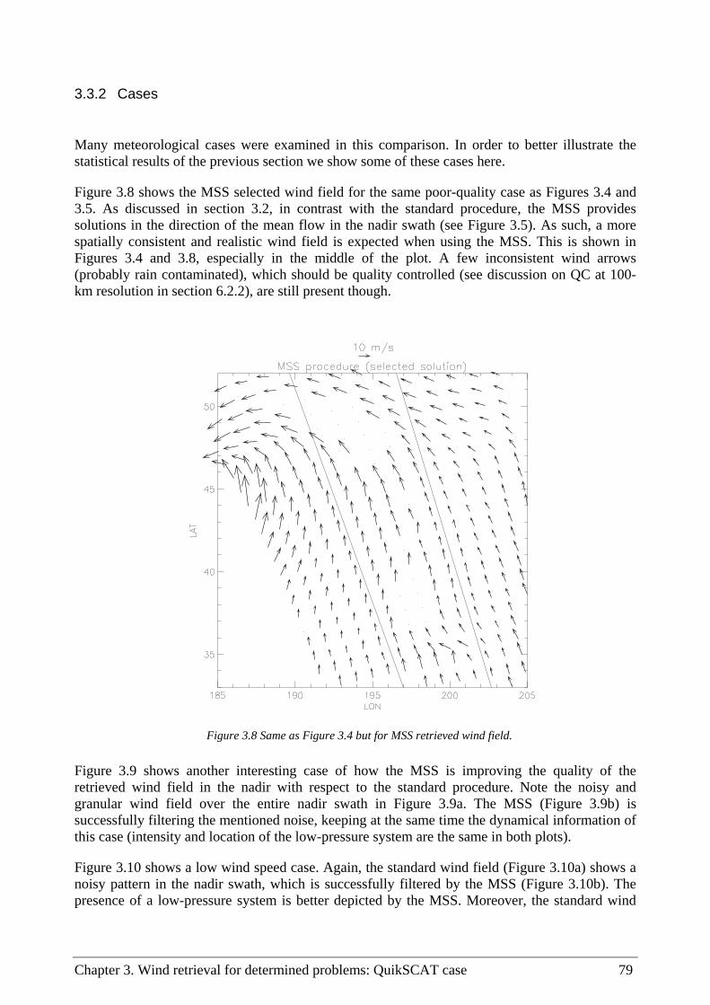
Chapter 3. Wind retrieval for determined problems: QuikSCAT case 79
3.3.2 Cases
Many meteorological cases were examined in this comparison. In order to better illustrate the statistical results of the previous section we show some of these cases here.
Figure 3.8 shows the MSS selected wind field for the same poor-quality case as Figures 3.4 and 3.5. As discussed in section 3.2, in contrast with the standard procedure, the MSS provides solutions in the direction of the mean flow in the nadir swath (see Figure 3.5). As such, a more spatially consistent and realistic wind field is expected when using the MSS. This is shown in Figures 3.4 and 3.8, especially in the middle of the plot. A few inconsistent wind arrows (probably rain contaminated), which should be quality controlled (see discussion on QC at 100-km resolution in section 6.2.2), are still present though.
Figure 3.9 shows another interesting case of how the MSS is improving the quality of the retrieved wind field in the nadir with respect to the standard procedure. Note the noisy and granular wind field over the entire nadir swath in Figure 3.9a. The MSS (Figure 3.9b) is successfully filtering the mentioned noise, keeping at the same time the dynamical information of this case (intensity and location of the low-pressure system are the same in both plots).
Figure 3.10 shows a low wind speed case. Again, the standard wind field (Figure 3.10a) shows a noisy pattern in the nadir swath, which is successfully filtered by the MSS (Figure 3.10b). The presence of a low-pressure system is better depicted by the MSS. Moreover, the standard wind
Figure 3.8 Same as Figure 3.4 but for MSS retrieved wind field.

80 Wind field retrieval from satellite radar systems
field is also somewhat noisy in the sweet swath, as expected from the low cost function modulation at low winds (see section 3.2). As it is discernible from Figure 3.10, the MSS is successfully filtering the noise in the sweet swath as well.
Figure 3.10c shows the ECMWF wind field. Both the intensity and location of the low-pressure system are in disagreement with the observations. The assimilation of a well-defined and spatially consistent wind field such as the MSS could help very much to improve ECMWF forecast.
3.4 Conclusions
After the extensive examination of the scatterometer and, in particular, the QuikSCAT inversion problems in chapter 2, the standard wind retrieval procedure is compared to a new procedure, the so-called multiple solution scheme, in this chapter. Prior to the comparison, several aspects of the wind retrieval are revised.
First, and in order to get a more suitable interface between the inversion and the AR schemes used in scatterometry, the MLE cost function is transformed into a probability cost function, by experimentally finding the relation between the MLE and the probability of the “true” wind. We use the determined probability function to predict how often a certain solution rank corresponds to the “true” solution, using ECMWF winds as reference. The correspondence is remarkable, indicating that the solution probability function we found is adequate.
a) b)
Figure 3.9 QuikSCAT retrieved wind field using the standard procedure (a) and the MSS (b). The acquisition date is February 3 2002 at 2 hours UTC. The solid lines separate the sweet-right (left side), the nadir (middle), and the sweet-left (right side) regions of the QuikSCAT swath.
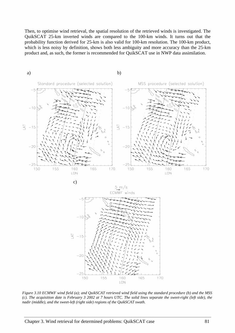
Chapter 3. Wind retrieval for determined problems: QuikSCAT case 81
Then, to optimise wind retrieval, the spatial resolution of the retrieved winds is investigated. The QuikSCAT 25-km inverted winds are compared to the 100-km winds. It turns out that the probability function derived for 25-km is also valid for 100-km resolution. The 100-km product, which is less noisy by definition, shows both less ambiguity and more accuracy than the 25-km product and, as such, the former is recommended for QuikSCAT use in NWP data assimilation.
a) b)
c)
Figure 3.10 ECMWF wind field (a); and QuikSCAT retrieved wind field using the standard procedure (b) and the MSS (c). The acquisition date is February 3 2002 at 7 hours UTC. The solid lines separate the sweet-right (left side), the nadir (middle), and the sweet-left (right side) regions of the QuikSCAT swath.

82 Wind field retrieval from satellite radar systems
The results of the extensive study on the QuikSCAT inversion problem (see chapter 2) show that in order to improve the wind retrieval, notably in the nadir region, more ambiguous wind solutions need to be provided to the AR. In order to be successful with a multiple solution concept, it is very important to characterize each of the ambiguous wind solutions with its corresponding probability of being the “true” wind. Therefore, a median filter AR, in which the probability of each solution is not explicitly used in the final selection, is inappropriate. We propose to use the multiple solution inversion output in combination with a variational analysis AR (i.e., 2D-Var), the so-called MSS. The variational analysis AR is not only capable of correctly assuming multiple solutions (it explicitly uses the probability) but also ensures spatial consistency and meteorological balance of the retrieved winds.
A comparison between the standard wind retrieval procedure and the MSS is then performed, using NCEP winds as background term for 2D-Var and ECMWF winds as validation reference. The MSS turns out to be more in agreement with ECMWF than the standard procedure, especially at nadir. As expected, the MSS wind direction is substantially better in nadir, thus validating the procedure proposed. Moreover, the MSS selected solution is, in general, probabilistically consistent, whereas the closest-to-NCEP solution is rather inconsistent with the a priori set probabilities. In other words, the influence of the background in the retrieved field is relatively small. As such, 2D-Var is successfully exploiting the information content of the observations.
The meteorological cases examined clearly show more spatially consistent and realistic wind fields for the MSS than for the standard procedure, especially at nadir. Moreover, the MSS is not only acting as a spatial filter, but is also keeping the wind information (e.g., lows, fronts, etc.) present in the observations. As such, the multiple solution scheme seems to be more appropriate for QuikSCAT data assimilation purposes than the standard scheme.
It may still be worthwhile to evaluate the effect of the spatial filtering by validating different versions of MSS with in-situ data.

Chapter 4. Wind retrieval for underdetermined problems: SAR case 83
Chapter 4
Wind Retrieval for Underdetermined Problems:
SAR Case
The wind retrieval of a single-view measurement system is underdetermined, i.e., an infinite number of wind solutions satisfy the GMF described by equation 1.5 (case a of section 1.4.1). As discussed in section 1.4.4, the ERS SAR instruments are well-calibrated single-view measurement systems and, as such, ideal to study the underdetermination problem.
As discussed in section 2.1.2, the MLE is a valid inversion parameter when the problem is determined. In the case of underdetermination, it is obvious that additional information is needed to derive the sea-surface wind field. This additional information can sometimes be derived from the SAR imaging system itself and/or from NWP models or buoy data.
In this chapter, several SAR wind retrieval algorithms will be described, and a comparison of two different wind retrieval methods will be performed: the first, widely used for SAR wind retrieval, assumes that the SAR system is not underdetermined and, as such, the wind direction information can be derived from the SAR image and then used in equation 1.5 (GMF) or equation 2.9 (MLE) to solve the wind speed component [note that both equations are equivalent for such purpose]; the second is an alternative we propose, which assumes that the SAR system is indeed underdetermined and, as such, combines the SAR wind information with additional information, i.e., NWP winds, to derive the wind field by using a statistical approach.
4.1 Current wind retrieval algorithms
In recent years, several algorithms have been developed and applied for SAR wind retrievals. Common among these are the C-band GMFs such as the CMOD-4 (Stoffelen and Anderson, 1993; Johannessen et al., 1994a) or the CMOD-Ifr (Ifremer, 1996), the SAR Wind Direction Algorithm (SWDA) (Wackerman et al., 1996, Vachon and Dobson, 1996, Fetterer et al., 1998), and the SAR Wind Algorithm (SWA) (Chapron et al., 1995, Kerbaol et al., 1998), which are all

84 Wind field retrieval from satellite radar systems
empirically based methods. A comprehensive presentation of these methods is found in Special Section on Advances in Oceanography and Sea Ice Research using ERS observations (JGR, 1998), EOQ (1998) and Fetterer et al. (1998).
As discussed in section 1.2.4, in the C-band models, the σ° is a non-linear function of wind speed (exponential) and wind direction (harmonic). For the ERS-1 scatterometer (whose data are used to develop the C-band models), three σ° views are available at each node (see section 1.3.1), allowing a solution of the CMOD-4 inversion to be obtained (case c of section 1.4.1) after taking account of the non-linearity (see scatterometer wind retrieval discussed in chapters 2 and 3). In contrast, inversion of a single-view SAR σ° measurement is more difficult as the sensitivity depends on the (unknown) true surface wind vector; one is therefore usually facing ambiguities and a problem of underdetermination (case a of section 1.4.1).
A limitation of the SWDA is that the spatial resolution of the wind direction information is derived from 25 km averages within the SAR image. Hence, at scales smaller than this, no wind direction information is available. In turn, all the σ° variability is incorrectly assigned to wind speed variability, by ignoring potential wind direction variability at these scales. Another problem of the SWDA is the 180° ambiguity in the wind direction determination, which is due to the fact that the wind streak reflects the orientation of the wind but not its sense of direction.
A limitation of the SWA is that the longer waves used to determine the smearing in the SAR image spectrum, are not fully coupled to local wind variations. In addition, as the wind waves and swell starts to feel the bottom topography as they move into shallow water, their period remains constant but their propagation direction change and the phase speed decreases. In turn, their wavelength decreases as well (Pond and Pickard, 1978). This leads to an underestimation of the SWA wind retrievals. Similar difficulties arise for offshore winds, in particular in shallow water, as the fetch and depth-limited waters affect the growth of the wave spectrum. As it, for a given wind speed, never reaches the spectrum for fully developed seas the SWA retrieval will underestimate the wind speed. Since the present study is focused on shallow water regions (mostly 100m depth or below), the wind field retrieval based on the SWA algorithm has been discarded.
We have chosen to apply SWDA and CMOD-4 inversion for further examination of the limitations addressed above. The algorithms are therefore briefly introduced below.
SAR Wind Direction Algorithm
The SWDA is used to extract the wind direction information from linear, low frequency expressions detected in the SAR image. These are usually associated with wind rows or wind streaks, which are manifestations of roll vortices in the Planetary Boundary Layer (PBL) (Brown, 1990; LeMone, 1973). The rolls are approximately aligned with the surface wind. Roll vortices in the PBL are counter-rotating helical circulation which are superimposed on the dominant wind field. They are most pronounced during unstable conditions (Wackerman et al., 1996), although Etling and Brown (1993) reported the presence of wind rolls in stable conditions as well. The SWDA was proposed by Fetterer et al. (1998) and looks for these linear expressions in the Fourier domain of the SAR image at a spatial resolution of 25 km to determine wind direction. Subsequently SAR wind speed is usually retrieved at smaller resolution.

Chapter 4. Wind retrieval for underdetermined problems: SAR case 85
C-band model inversion
The CMOD-4 model was originally developed for the ERS-1 scatterometer (Stoffelen and Anderson, 1993) but it has also shown to give reasonable estimates of wind speed when applied to ERS SAR images (Johannessen et al., 1994a). As discussed in section 1.2.4, the model is based on the backscatter from the rough ocean surface for moderate incidence angles (20°-60°), which is dominated by resonant Bragg scattering (Valenzuela, 1978). Additionally, specular reflection may contribute to the backscatter.
The CMOD-4 also follows the generic equation 1.5 described in section 1.2.4. The model is tuned to the real (“true”) wind at 10 meters height and the ERS-1 scatterometer σ°. CMOD-4 describes the coherence of the fore, aft and mid view backscatter measurement (the so-called cone surface) within about 0.1 dB. Wind retrieval based on CMOD-4 (Stoffelen and Anderson, 1997b) results in an accuracy of 3 m/s vector RMS (root mean square) when applied to scatterometer data (Stoffelen, 1998b). Other relevant references here include Korsbakken et al. (1998) and Lehner et al. (1998).
As discussed in section 1.3.2, to derive the wind field in a SAR precision image (PRI) from a C-band model inversion, comprehensive calibration of the radar backscatter value σ° is required (Scoon et al., 1996). The calibration procedure performed in this thesis can be found in Laur et al. (1998).
4.2 General approach
Besides the limitations of the different algorithms presented in the previous section, there is a very important problem inherent in SAR σ° observations. Both wind speed and wind direction information is present at the same time and cannot be properly discriminated. As discussed above, this underdetermination problem is obviously present in the wind vector retrieval algorithms, such as CMOD-4. Moreover, it directly affects the quality of the retrievals of the algorithms, which only derive one wind component, such as SWA or SWDA.
A methodology, which combines some of these algorithms with some external information, may be the solution to this inherent problem in SAR wind retrieval. In order to be successful, the method should take into account the spatial and accuracy characteristics and limitations of the observations and of the additional data used to combine them in an optimal way.
In this section, we consider an alternative approach by which the problem of underdetermination can be solved in a statistical way. The general statistical approach used by Lorenc (1986) to solve inversion problems (including underdetermined problems) in meteorological analysis is characterized by the most general equation of the Bayesian approach discussed in section 2.1.1; that is, the maximum a posterior probability described by equation 2.5. In contrast with scatterometers, where no external information is used in the prior probability P(xt), Lorenc (1986) uses background information, i.e., NWP. As such, P(xt) can be written as the deviations from (or errors of) some background xb:

86 Wind field retrieval from satellite radar systems
)()( bt xxx −= bPP (4.1)
Therefore, assuming Gaussian errors and that Pb and Pof (see equation 2.4) are independent, i.e., that background errors and observational errors are uncorrelated, equation 2.5 becomes:
)]()(2
1)}({)()}({
2
1exp[)( 11
bboo xxBxxxyFOxyx −−−−+−−∝ −− Tn
Tna kkP (4.2)
where O, F and B are the error covariance matrices of Pb, Po and Pf. respectively.; the first and second terms of the exponential are referred to as observation and background terms, respectively.
This equation allows combining the remotely sensed measurements (observation term) and the external information (background term) in a statistical way. In other words, it allows to combine the SAR information, i.e., σ° and/or wind streaks, with some background information, i.e., NWP models and/or buoy data, to retrieve the most probable wind vector, assuming that all sources of information contain (Gaussian) errors and these are well characterized, including their spatial correlation.
The most probable wind vector results from maximizing Pa (equation 4.2), which is equivalent to minimizing –ln(Pa):
)()()}({)()}({ 11bboo xxBxxxyFOxy −−+−+−= −− T
nT
n kkJ (4.3)
where J is the so-called cost function.
In case of a non-linear forward model Kn or in case of non-linear error properties, e.g., the error magnitude depending on the value of the true observation, the maximum posterior probability solution may have some unwanted features, such as biases (see, e.g., Stoffelen and Anderson, 1997b). It is important in these cases to carefully investigate whether the best estimate comes from the maximum probability or from other optimization techniques (see beginning of chapter 2), such as the minimum variance or the unbiased analysis (Stoffelen, 2000).
SAR Application
For SAR, yo can contain σ°, wind direction from wind streaks or other derived parameters (see section 4.1); kn can be the C-band model, the SWDA or other SAR wind retrieval algorithm (see section 4.1); xb can be a NWP wind field or buoy wind data; and x is the wind field at 10m height.
The matrices O+F and B can be diagonal in which case the global minimisation problem is just a sum of local minimisation problems. In meteorological analyses, B is constructed generally from so-called spatial structure functions that provide the spatial error correlation of the background field. Since the observational network is generally rather sparse, the typical correlation length used for wind parameters is 250 km. Unless in specific cases of katabatic flow, land breeze, etc, that may provide a well-determined physical forcing, the scarcity of the observation network is also a problem for high-resolution models, such as the High-resolution limited area model (HIRLAM). So, generally over a SAR scene the NWP output will be quite smooth.
Chapter 4. Wind retrieval for underdetermined problems: SAR case 87
Also, the O matrix may contain correlation. A good example is the case where SAR image wind streaks are used for wind direction determination (see section 4.1). A spatial context of 25 km is used for this (Fetterer et al., 1998), and if the wind state from SAR at, let’s say, 5 km resolution is sought, then the contribution from the wind streak observations is spatially correlated.
For SAR, several existing wind retrieval methods can be described by the above formalism. Generally, further simplifying assumptions have to be made such as B→∞ or O + F = I (identity).
4.3 Evaluation of two SAR wind retrieval methods
In this section, we evaluate the outcome of two different SAR wind retrieval methods. The first one is based on a commonly used combination of the SWDA and C-band models, whereas the second one is the new method based on the generalized inverse approach addressed in section 4.2. This new method, called the Statistical Wind Retrieval Approach (SWRA) combines the SAR derived wind information with the VHR (very-high resolution HIRLAM) output to determine the optimum wind vector, using a simplified set of assumptions. Unlike the other methods, this method takes into account the relative quality of the observations (SAR) and the background information (VHR). A description of the data used in here is presented prior to the evaluation.
4.3.1 SAR and HIRLAM data
A set of 15 SAR images that were acquired from January 1997 to October 1997 by the second European Remote Sensing Satellite (ERS-2) over the southern North Sea coastal regions were selected representing various wind conditions (onshore, offshore, along-shore, low, medium, high). The ERS-2 SAR PRI images presented in this paper are provided by ESA (Grabak and Laur, 1995). All SAR acquisition times are between 10:00 UTC and 11:00 UTC. The selected SAR images are listed in table 4.1.
HIRLAM V55, a high-resolution (55 km) mesoscale NWP model, is run operationally at KNMI. It has the capability of running a nested VHR (Very High Resolution) model with a 5 km resolution, which is able to simulate and generate specific mesoscale atmospheric weather phenomena such as land-sea breezes (De Bruijn, 1997). This model yields as output, among others, the wind field at 10 m height above the sea surface, which can be compared or combined with the near surface wind information inferred from the SAR images.
A comprehensive description of HIRLAM and its nesting strategy can be found in De Bruijn and Brandsma (2000). However, it is important to mention that the analysis is performed on the V55 model; the nested model does not have its own analysis scheme and receives its initial information from the coarse mesh model. There are no specific physical parameterisation schemes for the VHR model. [A complete description of such schemes is found in Gustafson (1991)].

88 Wind field retrieval from satellite radar systems
Table 4.1 ERS-2 PRI SAR images selected.
Orbit Frame Acquisition date Acquisition time (UTC)
Wind Conditions1
9381 2529 4-Feb-97 10:48:56 H / Off
9567 2511 17-Feb-97 10:40:04 M / Along
9610 2547 20-Feb-97 10:46:20 M / Off
10297 2511 9-Apr-97 10:37:13 L / Along
10569 2547 28-Apr-97 10:40:34 M / On
10984 2511 27-May-97 10:28:37 M / On
11428 2511 27-Jun-97 10:54:30 H / Along
11614 2547 10-Jul-97 10:46:23 L / Along
12072 2547 11-Aug-97 10:40:37 L / Off
12301 2511 27-Aug-97 10:37:14 L / Off
12430 2511 5-Sep-97 10:54:28 M / Off
12487 2511 9-Sep-97 10:28:35 H / On
12530 2511 12-Sep-97 10:34:19 M / Along
12931 2511 10-Oct-97 10:54:29 H / Off
12988 2511 14-Oct-97 10:28:37 L / On 1 L: Low winds (<7 m/s); M: Medium winds (7 m/s<v<13 m/s); H: High winds (>13 m/s) On: Onshore winds; Off: Offshore winds; Along: Alongshore winds
In order to collocate the HIRLAM output product to the calibrated SAR (including analogue to digital converter power loss correction) image at a standard size of 80 km x 95 km, we define a WVC in the SAR image, as an area of 5km x 5km only covered by ocean (no land or ice “contamination”). In a pure ocean calibrated SAR image, there is a total of 304 (16 x 19) WVCs. Then, the HIRLAM output product is spatially interpolated to the actual coordinates of the WVCs. Finally, as HIRLAM forecasts are provided on an hourly basis, the HIRLAM outputs are linearly interpolated to the actual acquisition time of the SAR image.
4.3.2 SWDA+C-band method
In this section, we explore a common way of deriving wind vectors based on a combination of one of the C-band models and the SWDA, with the additional help of the VHR HIRLAM wind direction information.

Chapter 4. Wind retrieval for underdetermined problems: SAR case 89
4.3.2.1 Methodology
As described in Fetterer et al. (1998), the SWDA is used to retrieve the wind direction from the streak features in the SAR image, which are approximately aligned in the direction of the surface wind. As emphasised in section 4.1, the retrieval method only provides estimate of the wind streak direction, and therefore a 180° ambiguity remains. In contrast with Fetterer et al. (1998) who use buoy data to provide the additional information needed to solve this ambiguity, we use the VHR model, i.e., the direction value closest to that given by the VHR is selected.
The SWDA provides wind direction information in 25-km grid cells. In order to retrieve a wind vector of 5 km resolution (VHR model resolution), the 25 km cells are subdivided in 5 km WVCs, assuming a constant and error-free wind direction within the 25 km area. The CMOD-4 is then used to retrieve the wind speed at each WVC based on the σ°, the incidence angle and the SWDA wind direction information. We computed wind speed in an area of 3 x 3 25-km grid cells at 5-km resolution.
As said in section 4.2, the SAR wind retrieval methods can be described by the general approach while varying the set of assumptions. Therefore, this alternative method can also be described following the general approach, but with a very strong set of assumptions, notably: no errors, and no background term in the cost function.
4.3.2.2 Validation procedure
Although the quantitative validation is done with the VHR model wind information as a reference, a method based on an optimum combination of both VHR and C-band models is also used to qualitatively analyse some specific cases. In so doing one can alternatively retrieve the wind speed or the wind direction from the C-band model, using the VHR wind direction or wind speed products as input. In the latter case, when wind direction is retrieved, four ambiguities are generally found (i.e., up to four points in the solid line of Figure 1.8a satisfy a given wind speed solution) from which the closest to the VHR direction is selected. The RMS difference of the retrieved wind vector component compared to the VHR component can then be estimated:
N
vvRMS
N
i
tii∑
=
−= 1
2)( (4.4)
where vi and vit correspond to the wind vector component for a particular WVC provided by the
C-band and the VHR models respectively; and N is the number of WVCs in the SAR image.
The method, described by Portabella (1998), uses variations around the input VHR values to look for the minimum RMS. In the case of wind speed retrievals, the variations are performed in the VHR wind direction, looking for a minimum RMS in wind speed; and similarly, in the case of
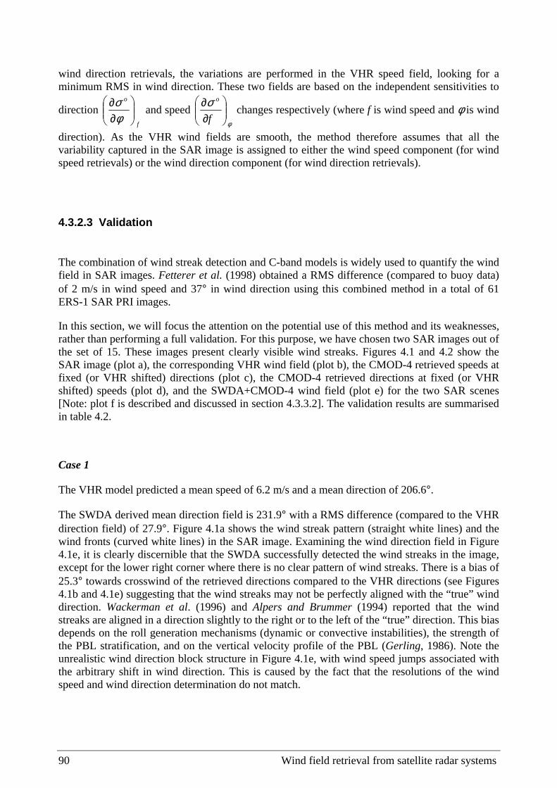
90 Wind field retrieval from satellite radar systems
wind direction retrievals, the variations are performed in the VHR speed field, looking for a minimum RMS in wind direction. These two fields are based on the independent sensitivities to
direction f
o
∂∂
φσ
and speed φ
σ
∂∂
f
o
changes respectively (where f is wind speed and φ is wind
direction). As the VHR wind fields are smooth, the method therefore assumes that all the variability captured in the SAR image is assigned to either the wind speed component (for wind speed retrievals) or the wind direction component (for wind direction retrievals).
4.3.2.3 Validation
The combination of wind streak detection and C-band models is widely used to quantify the wind field in SAR images. Fetterer et al. (1998) obtained a RMS difference (compared to buoy data) of 2 m/s in wind speed and 37° in wind direction using this combined method in a total of 61 ERS-1 SAR PRI images.
In this section, we will focus the attention on the potential use of this method and its weaknesses, rather than performing a full validation. For this purpose, we have chosen two SAR images out of the set of 15. These images present clearly visible wind streaks. Figures 4.1 and 4.2 show the SAR image (plot a), the corresponding VHR wind field (plot b), the CMOD-4 retrieved speeds at fixed (or VHR shifted) directions (plot c), the CMOD-4 retrieved directions at fixed (or VHR shifted) speeds (plot d), and the SWDA+CMOD-4 wind field (plot e) for the two SAR scenes [Note: plot f is described and discussed in section 4.3.3.2]. The validation results are summarised in table 4.2.
Case 1
The VHR model predicted a mean speed of 6.2 m/s and a mean direction of 206.6°.
The SWDA derived mean direction field is 231.9° with a RMS difference (compared to the VHR direction field) of 27.9°. Figure 4.1a shows the wind streak pattern (straight white lines) and the wind fronts (curved white lines) in the SAR image. Examining the wind direction field in Figure 4.1e, it is clearly discernible that the SWDA successfully detected the wind streaks in the image, except for the lower right corner where there is no clear pattern of wind streaks. There is a bias of 25.3° towards crosswind of the retrieved directions compared to the VHR directions (see Figures 4.1b and 4.1e) suggesting that the wind streaks may not be perfectly aligned with the “true” wind direction. Wackerman et al. (1996) and Alpers and Brummer (1994) reported that the wind streaks are aligned in a direction slightly to the right or to the left of the “true” direction. This bias depends on the roll generation mechanisms (dynamic or convective instabilities), the strength of the PBL stratification, and on the vertical velocity profile of the PBL (Gerling, 1986). Note the unrealistic wind direction block structure in Figure 4.1e, with wind speed jumps associated with the arbitrary shift in wind direction. This is caused by the fact that the resolutions of the wind speed and wind direction determination do not match.

Chapter 4. Wind retrieval for underdetermined problems: SAR case 91
The CMOD-4 derived mean wind speed field is 5.1 m/s with a RMS difference of 1.7 m/s. It is discernible from Figure 4.1e that in the areas where the wind direction estimates are biased towards crosswind compared to VHR directions (Figure 4.1b), wind speed estimates are high compared to VHR speeds. This documents, as expected, that C-band model errors are directly affected by the errors in the direction estimation, i.e., a direction bias towards crosswinds will produce an overestimation of C-band wind speeds and a bias towards upwind or downwind will produce underestimation in the C-band speeds.
Despite this bias, the wind speed field retrieved from the C-band model suggests the presence of wind fronts, which are not detected by the VHR model. The upper right corner of the image (Figure 4.1e) corresponds to the higher wind speed part of the front (about 8 m/s). In the lower left corner of the image there is also an increase of the wind speed, suggesting the presence of a second somewhat weaker front. This is also the case for the retrieved wind speeds at fixed directions in Figure 4.1c, where the fronts can be seen as a wind speed change. In comparison, the retrieved wind direction at fixed speed (Figure 4.1d) also shows the wind front, but by a change in wind direction. According to the wind streak information, Figure 4.1c is more realistic than Figure 4.1d, although it is likely that both retrieval methods contain errors due to the strict assumptions of σ° variability as either wind speed or wind direction variations.
Case 2
The VHR model predicted a mean speed of 12.6 m/s and a mean direction of 322.9°.
The SWDA mean direction field is 323.9° and the RMS difference is 16.5°. Figure 4.2a shows the wind streaks (straight lines) in the SAR image. Although there is no significant bias in this case, the image presents some variability in the wind direction. In particular, the wind streaks are changing direction in the right part of the image (straight black lines), suggesting the presence of a wind front (curved black line), which is not predicted by the VHR model. To the left of the front, the wind streak directions are biased about 15° towards upwind when compared to the VHR directions (see Figures 4.2b and 4.2e). This is due to the fact that the precision of the SWDA is affected by the sampling of the SAR scene in the Fourier domain. Fetterer et al. (1998) reported that the precision of the direction estimate decreases as the location of the peak gets closer to the origin of the Fourier domain. In particular, for wind streaks with spacing from 4.5 to 6 km an angle precision up to 27° was reported. In the lower left corner of the SAR image, the wind streak spacing is 4.5 km, leading to a discretization of 27° in the wind streak direction determination. Note again the arbitrary blocked structure of the wind field.
The CMOD-4 derived mean speed field is 10.7 m/s and the RMS is 2.8 m/s. The relatively high RMS value indicates a significant variability due to the presence of the wind front. The wind direction field in the right part of the wind front (Figure 4.2e) is slightly biased towards crosswind compared to the C-band retrieved directions at fixed speeds in Figure 4.2d. On the other hand, the C-band retrieved speeds at fixed directions of Figure 4.2c decrease at the right side of the front. Therefore, the increase in wind speed to the right of the front (2-3 m/s higher than the left part) in Figure 4.2e is mainly due to a misalignment of the wind streaks with respect to the “true” direction field. In the lower left corner of the image (Figure 4.2e), the speeds are higher than in the surrounding 25-km wind direction grid cells. The reason is the error in the wind direction estimation due to the streak spacing. This error is biasing the direction towards

92 Wind field retrieval from satellite radar systems
crosswind in this particular 25-km cell, which in turn produces higher C-band retrieved wind speeds than in the surrounding 25-km cells.
In contrast with the previous image (case 1), the retrieved directions at fixed speeds (Figure 4.2d) are more realistic than the retrieved speeds at fixed directions (Figure 4.2c) according to the wind streak information.
Summary of all cases
From the set of 15 SAR images, only four of them contained clear wind streaks and therefore used to examine the combined SWDA + C-band method. The two cases not shown present similar problems to the two above discussed cases, although slightly better agreement with the VHR as no fronts are present in the scenes. This retrieval method is able to detect some atmospheric phenomena, like wind fronts, which are not predicted by the VHR model. However, the accuracy of the SWDA decreases with the wind streak spacing and the wind streaks show indeed some misalignment with the “true” wind direction. The C-band model errors are directly affected by the errors in the direction estimation. Due to the low resolution of the direction retrievals, all the variability in the 25-km cells is assumed to be in the speed component, which is obviously incorrect. Finally, the direction of the local wind is not always detected hence limiting the full use of the method1. We further investigate these cases in the next section.
1 Note that in this analysis, we have used the “peak” method to retrieve wind directions. This method simply finds the position with the highest value and assumes that this represents a peak in the spectrum due to wind streaks. Direction is assumed to be normal to the peak direction. However, Fetterer et al. (1998) also used a more sophisticated method to look for the wind direction in the Fourier domain. This second method is called “cigar-shaped” and assumes that the wind direction is manifested in the spectrum as a smear of energy in the crosswind direction. This method was reported to be very useful, as it was able to detect not only wind streaks but also other manifestations of the local wind. Surfactant streaks (at low wind speed), blowing foam and water from breaking waves (at high wind speed), and ellipticity of atmospheric convective cells will give rise to image expressions that are aligned with the local surface wind direction. This, in turn, will generate smears in the “cigar-shaped” spectrum. Fetterer et al. (1998) detected smears in the spectrum in all 61 ERS-1 SAR images examined.
Table 4.2 Validation SWDA+CMOD-4.
SAR Scene
VHR Mean Speed (m/s) / Direction (°)
RMS in Speed (m/s) / Direction (°)
Bias in Speed (m/s) / Direction (°)
Case 1 6.2 / 206.6 1.7 / 27.9 -1.1 / 25.3
Case 2 12.6 / 322.9 2.8 / 16.5 -1.9 / 1
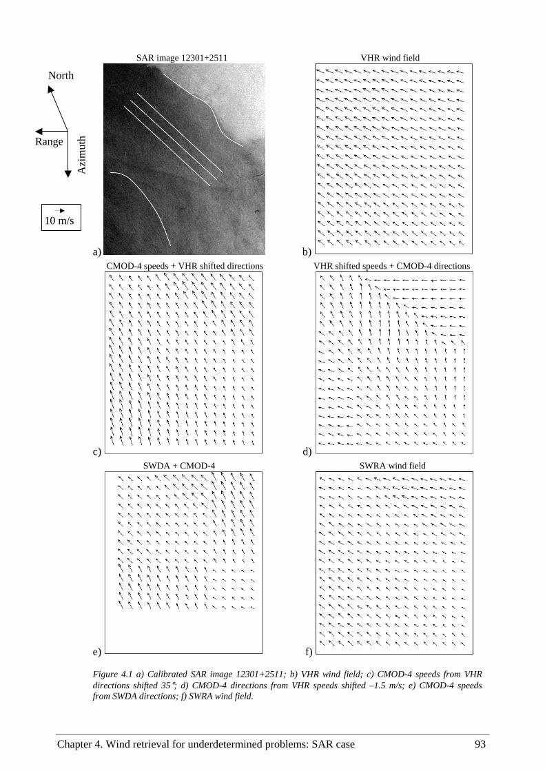
Chapter 4. Wind retrieval for underdetermined problems: SAR case 93
SAR image 12301+2511 VHR wind field
a) b)
CMOD-4 speeds + VHR shifted directions VHR shifted speeds + CMOD-4 directions
c) d)
SWDA + CMOD-4 SWRA wind field
e) f)
Figure 4.1 a) Calibrated SAR image 12301+2511; b) VHR wind field; c) CMOD-4 speeds from VHR directions shifted 35°; d) CMOD-4 directions from VHR speeds shifted –1.5 m/s; e) CMOD-4 speeds from SWDA directions; f) SWRA wind field.
Azi
mut
h North
Range
10 m/s

94 Wind field retrieval from satellite radar systems
SAR image 12530+2511 VHR wind field
a) b)
CMOD-4 speeds + VHR shifted directions VHR shifted speeds + CMOD-4 directions
c) d)
SWDA + CMOD-4 SWRA wind field
e) f)
Figure 4.2 a) Calibrated SAR image 12530+2511; b) VHR wind field; c) CMOD-4 speeds from VHR directions shifted -15°; d) CMOD-4 directions from VHR speeds shifted –1.5 m/s; e) CMOD-4 speeds from SWDA directions; f) SWRA wind field.
Range
North A
zim
uth
5 m/s

Chapter 4. Wind retrieval for underdetermined problems: SAR case 95
4.3.3 Statistical wind retrieval approach
As explained in section 4.2, the method derived from the general approach will depend on the set of assumptions we make. Here we present a simplified statistical method consisting of combining SAR data and VHR wind to retrieve an optimum wind vector. In contrast with section 4.3.2, it assumes that both the SAR observations (including the retrieval algorithms) and the VHR model output contain errors.
4.3.3.1 Methodology
The method uses a C-band model function as forward model to relate the SAR measured (and calibrated) backscatter to the wind state, and the VHR wind field as background information.
Therefore, equation 4.3 can be written as:
)()()}({)()}({ 11HH vvBvvvFOv −−+−+−= −− To
mTo
m CMODCMODJ σσ (4.5)
where σm° are the backscatter measurements, CMOD the C-band model function, vH the HIRLAM VHR wind field, and v the wind field estimate.
For simplicity, we assume that there is no spatial correlation (O+F and B are diagonal matrices), and therefore the global minimisation problem can be treated as a sum of local minimisation problems. In other words, we can minimize the cost function J for every 5-km WVC, instead of minimizing the entire SAR scene. Therefore, for every WVC the cost function we have to minimize is:
22
∆−
+
∆−
=v
vv H
σσσ oo
mJ (4.6)
where σ° is the backscatter value computed by applying the C-band model with the wind vector estimate v and incidence angle θ corresponding to that particular WVC [σ°=CMOD(v)θ]; ∆σ and ∆v are the Gaussian error SDs from the O and B matrices respectively. For simplicity, the forward model has been considered perfect (F=0).
Assuming that the wind vector component errors are independent, equation 4.6 can be written as:
222
∆−
+
∆−
+
∆−
=v
vv
u
uuJ HH
oom
σσσ
(4.7)
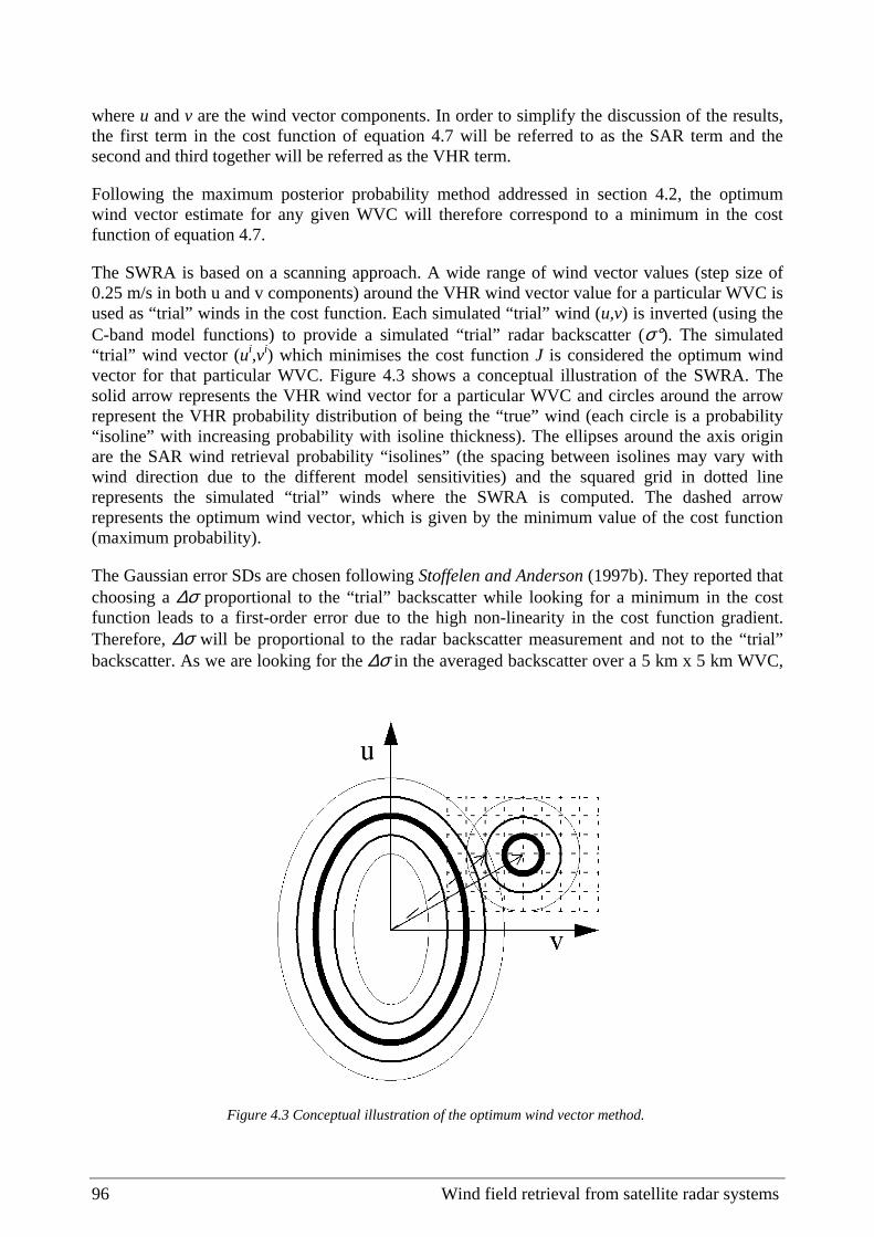
96 Wind field retrieval from satellite radar systems
where u and v are the wind vector components. In order to simplify the discussion of the results, the first term in the cost function of equation 4.7 will be referred to as the SAR term and the second and third together will be referred as the VHR term.
Following the maximum posterior probability method addressed in section 4.2, the optimum wind vector estimate for any given WVC will therefore correspond to a minimum in the cost function of equation 4.7.
The SWRA is based on a scanning approach. A wide range of wind vector values (step size of 0.25 m/s in both u and v components) around the VHR wind vector value for a particular WVC is used as “trial” winds in the cost function. Each simulated “trial” wind (u,v) is inverted (using the C-band model functions) to provide a simulated “trial” radar backscatter (σ°). The simulated “trial” wind vector (ui,vi) which minimises the cost function J is considered the optimum wind vector for that particular WVC. Figure 4.3 shows a conceptual illustration of the SWRA. The solid arrow represents the VHR wind vector for a particular WVC and circles around the arrow represent the VHR probability distribution of being the “true” wind (each circle is a probability “isoline” with increasing probability with isoline thickness). The ellipses around the axis origin are the SAR wind retrieval probability “isolines” (the spacing between isolines may vary with wind direction due to the different model sensitivities) and the squared grid in dotted line represents the simulated “trial” winds where the SWRA is computed. The dashed arrow represents the optimum wind vector, which is given by the minimum value of the cost function (maximum probability).
The Gaussian error SDs are chosen following Stoffelen and Anderson (1997b). They reported that choosing a ∆σ proportional to the “trial” backscatter while looking for a minimum in the cost function leads to a first-order error due to the high non-linearity in the cost function gradient. Therefore, ∆σ will be proportional to the radar backscatter measurement and not to the “trial” backscatter. As we are looking for the ∆σ in the averaged backscatter over a 5 km x 5 km WVC,
Figure 4.3 Conceptual illustration of the optimum wind vector method.

Chapter 4. Wind retrieval for underdetermined problems: SAR case 97
this value should be closely associated with the variability in the backscatter measurement (instrument error + geophysical error) from 0 to 5 km (subcell variability). The subcell averaged mean SD for all the set of 15 SAR images is 7.8% (see Portabella, 1998) and is used as the proportionality constant, i.e., ∆σ = 0.078σm°.
∆u and ∆v represent the error of the HIRLAM model at 5 km resolution. At present no attempt has been done on calculating these errors, and since the HIRLAM is close to ECMWF, we use the ECMWF errors instead. Stoffelen (1996) reported a large scale (250 km) error variance in both ECMWF wind components (u,v) of approximately 1 m2/s2. Stoffelen and Anderson (1997b) use a climatological wind spectrum to estimate the small-scale variability. They find that the computed variabilities are consistent with differences between measurement systems with different resolution, i.e., buoys, scatterometer and ECMWF model. Using their climatological spectrum, we estimate the variability between 5 and 250 km to be 2.0 m2/s2, leading to a final total error variance of 3 m2/s2 in both wind components. Therefore, ∆u=∆v= 3 m/s.
4.3.3.2 Results
Table 4.3 shows the averaged variability in both wind components (the wind direction variability is given in equivalent m/s) for all the VHR, SWRA and C-band retrieved wind fields. The latter is computed by using a VHR wind speed (direction) as input to retrieve the wind direction (speed) with the C-band model.
The variability in the C-band retrieved winds fields is, as expected, much higher than the variability in the VHR wind fields due to the impact of short scale atmospheric phenomena which are not included in the VHR model. The fact that the VHR model does not have its own analysis scheme, that it receives its initial information from the V55 model, and that there are no specific parameterisation schemes for the VHR model (see section 4.3.1), makes the VHR effective resolution closer to 55 km than to 5 km.
Similarly, table 4.3 shows low variability in the SWRA wind directions, comparable to the variability in the VHR wind fields and much lower than the variability in the C-band models retrieved wind directions. On the other hand, the variability in the SWRA wind speeds is between the low variability of the VHR speeds and the higher variability of the C-band retrieved speeds. For small-scale turbulence, as depicted in SAR images, one may expect the same amount of variability along and perpendicular to the mean flow (i.e., in the speed and direction component). VHR contains the large scales (about 100 km) and the SAR term is effective in adding smaller scale (5 km) variability when a discrepancy occurs. This variability is added to the component
Table 4.3 Averaged STD comparisons.
Wind Component VHR Averaged STD
SWRA Averaged STD
CMOD-4 Averaged STD
Speed (m/s) 0.55 0.75 1
Direction (m/s)1 0.45 0.45 1.65 1 The direction values are given in equivalent m/s.
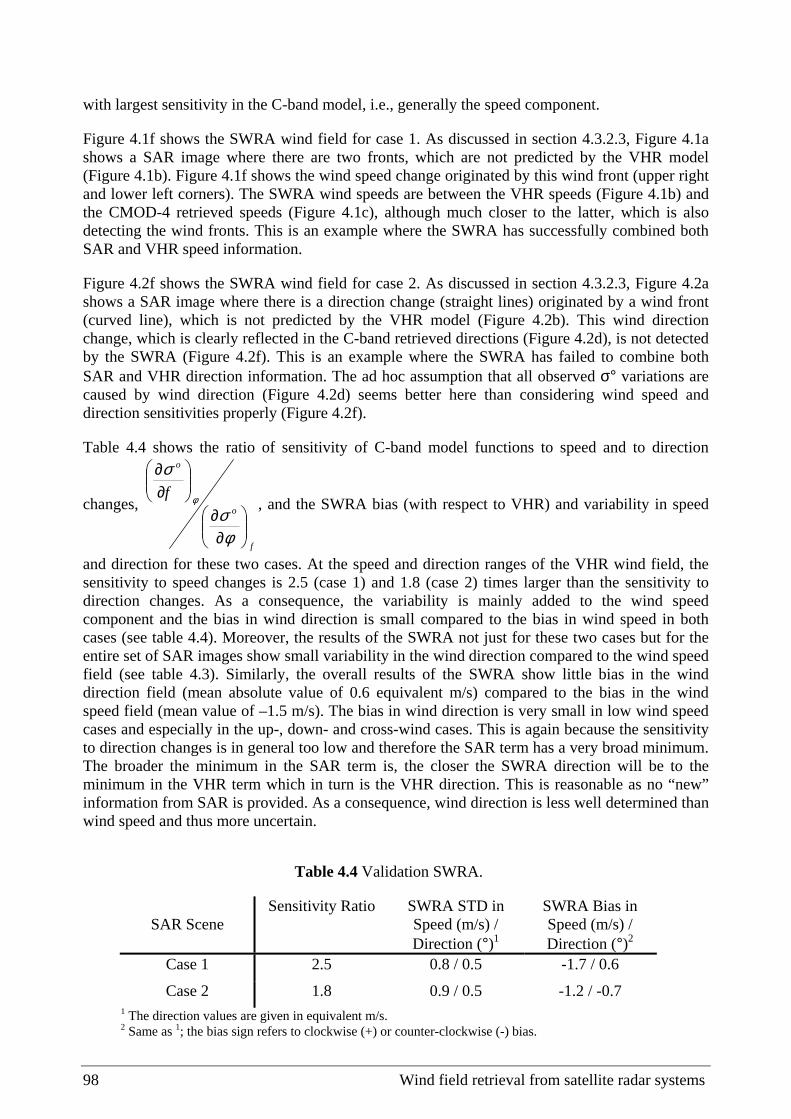
98 Wind field retrieval from satellite radar systems
with largest sensitivity in the C-band model, i.e., generally the speed component.
Figure 4.1f shows the SWRA wind field for case 1. As discussed in section 4.3.2.3, Figure 4.1a shows a SAR image where there are two fronts, which are not predicted by the VHR model (Figure 4.1b). Figure 4.1f shows the wind speed change originated by this wind front (upper right and lower left corners). The SWRA wind speeds are between the VHR speeds (Figure 4.1b) and the CMOD-4 retrieved speeds (Figure 4.1c), although much closer to the latter, which is also detecting the wind fronts. This is an example where the SWRA has successfully combined both SAR and VHR speed information.
Figure 4.2f shows the SWRA wind field for case 2. As discussed in section 4.3.2.3, Figure 4.2a shows a SAR image where there is a direction change (straight lines) originated by a wind front (curved line), which is not predicted by the VHR model (Figure 4.2b). This wind direction change, which is clearly reflected in the C-band retrieved directions (Figure 4.2d), is not detected by the SWRA (Figure 4.2f). This is an example where the SWRA has failed to combine both SAR and VHR direction information. The ad hoc assumption that all observed σ° variations are caused by wind direction (Figure 4.2d) seems better here than considering wind speed and direction sensitivities properly (Figure 4.2f).
Table 4.4 shows the ratio of sensitivity of C-band model functions to speed and to direction
changes,
f
o
o
f
∂∂
∂∂
φσ
σ
φ , and the SWRA bias (with respect to VHR) and variability in speed
and direction for these two cases. At the speed and direction ranges of the VHR wind field, the sensitivity to speed changes is 2.5 (case 1) and 1.8 (case 2) times larger than the sensitivity to direction changes. As a consequence, the variability is mainly added to the wind speed component and the bias in wind direction is small compared to the bias in wind speed in both cases (see table 4.4). Moreover, the results of the SWRA not just for these two cases but for the entire set of SAR images show small variability in the wind direction compared to the wind speed field (see table 4.3). Similarly, the overall results of the SWRA show little bias in the wind direction field (mean absolute value of 0.6 equivalent m/s) compared to the bias in the wind speed field (mean value of –1.5 m/s). The bias in wind direction is very small in low wind speed cases and especially in the up-, down- and cross-wind cases. This is again because the sensitivity to direction changes is in general too low and therefore the SAR term has a very broad minimum. The broader the minimum in the SAR term is, the closer the SWRA direction will be to the minimum in the VHR term which in turn is the VHR direction. This is reasonable as no “new” information from SAR is provided. As a consequence, wind direction is less well determined than wind speed and thus more uncertain.
Table 4.4 Validation SWRA.
SAR Scene
Sensitivity Ratio SWRA STD in Speed (m/s) / Direction (°)1
SWRA Bias in Speed (m/s) / Direction (°)2
Case 1 2.5 0.8 / 0.5 -1.7 / 0.6
Case 2 1.8 0.9 / 0.5 -1.2 / -0.7 1 The direction values are given in equivalent m/s. 2 Same as 1; the bias sign refers to clockwise (+) or counter-clockwise (-) bias.

Chapter 4. Wind retrieval for underdetermined problems: SAR case 99
In summary, it seems that the SWRA is successfully combining the SAR and the VHR speed information. In comparison it is systematically adding less variability to the wind direction, biasing the results towards the VHR direction information, since the SAR radar backscatter is generally most sensitive to wind speed variations.
Using the information on wind streaks, one may conclude that the backscatter variability in Figure 4.2a is caused by the wind direction rather than the wind speed changes. In order to improve the SWRA performance, an additional wind streak term may be added after investigation of its weight (additional terms in matrix O+F) as a measure of the quality of the SAR-derived wind direction. Improved wind direction determination will result in improved wind speed retrieval. Furthermore, in meteorological analysis spatial correlation patterns (matrix B) are used to prescribe the amount of rotation and divergence in the analysed field. We anticipate that the dominating rotational part would constrain the solution of the SWRA in the appropriate direction. However, we did not test this.
4.3.3.3 Error Analysis
In the SWRA, it is assumed that SAR σ° variability may be due to speed and direction changes. The relative quality of VHR and SAR data is weighted in the analysis, taking into account the information content of the data. Nonetheless, non-linearities in the C-band model functions and inaccuracies in the cost function weights (∆σ2,⋅∆u2 and⋅∆v2) introduce errors in the wind vector estimation. As said in section 4.2, the best retrieval method (minimum variance, maximum probability, unbiased) will depend on the errors induced by the non-linearity of the forward model.
In order to estimate non-linearity errors in the SWRA, the following error analysis is performed. From a “true” wind vector (ut,vt) we apply the C-band model function to get a “true” radar backscatter σt° at a mean incidence angle of 23°. Then, we add the Gaussian noise corresponding to the values of⋅∆u,⋅∆v and ∆σ discussed in section 4.3.3.1 to generate the VHR wind vectors vH
i=(uti,vt
i) and the backscatter measurements σmoi. For each pair [vH
i, σmoi] we compute an
SWRA wind vector (see section 4.3.3.1). Finally, we compute the bias of SWRA winds with respect to the “true” wind in speed and direction components.
This procedure is performed for different “true” wind speeds and directions, ranging from 5 to 15 m/s (step size of 5 m/s) and from 0° to 180° (step size of 10°) [note: the rest of the angles is not computed because of symmetry].
Figure 4.4 shows the wind speed and direction bias results in the SWRA. A positive bias in wind speed component denotes an underestimation of the SWRA with respect to the “true” wind speed and vice versa. Both a positive direction bias in the range of “true” wind directions 0°-90° and a negative bias in the range 90°-180° denote a bias towards crosswind (0° is upwind). In contrast, both a negative direction bias in the range 0°-90° and a positive direction bias in the range 90°-180° denote a up/down-wind bias.
The biases in wind speed component are always positive, denoting underestimation, and with a maximum around crosswind directions. Moreover, the underestimation increases with decreasing
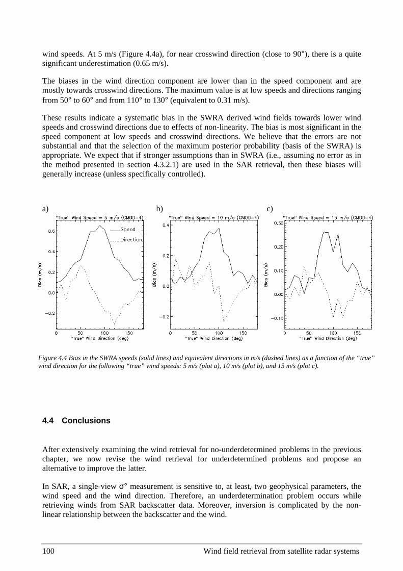
100 Wind field retrieval from satellite radar systems
wind speeds. At 5 m/s (Figure 4.4a), for near crosswind direction (close to 90°), there is a quite significant underestimation (0.65 m/s).
The biases in the wind direction component are lower than in the speed component and are mostly towards crosswind directions. The maximum value is at low speeds and directions ranging from 50° to 60° and from 110° to 130° (equivalent to 0.31 m/s).
These results indicate a systematic bias in the SWRA derived wind fields towards lower wind speeds and crosswind directions due to effects of non-linearity. The bias is most significant in the speed component at low speeds and crosswind directions. We believe that the errors are not substantial and that the selection of the maximum posterior probability (basis of the SWRA) is appropriate. We expect that if stronger assumptions than in SWRA (i.e., assuming no error as in the method presented in section 4.3.2.1) are used in the SAR retrieval, then these biases will generally increase (unless specifically controlled).
4.4 Conclusions
After extensively examining the wind retrieval for no-underdetermined problems in the previous chapter, we now revise the wind retrieval for underdetermined problems and propose an alternative to improve the latter.
In SAR, a single-view σ° measurement is sensitive to, at least, two geophysical parameters, the wind speed and the wind direction. Therefore, an underdetermination problem occurs while retrieving winds from SAR backscatter data. Moreover, inversion is complicated by the non-linear relationship between the backscatter and the wind.
a) b) c)
Figure 4.4 Bias in the SWRA speeds (solid lines) and equivalent directions in m/s (dashed lines) as a function of the “true” wind direction for the following “true” wind speeds: 5 m/s (plot a), 10 m/s (plot b), and 15 m/s (plot c).

Chapter 4. Wind retrieval for underdetermined problems: SAR case 101
A commonly used method, which combines the SAR image streak information (SWDA) and the SAR backscatter information (CMOD-4), is first examined. The combination of the SWDA with the CMOD-4 closes the problem, but does not take account of the difference in spatial context of the SAR σ° and the wind streak information. Moreover, uncertainties in wind streak determination and σ° are not explicitly used in the wind interpretation.
In addition, the following uncertainties have been reported from the SWDA: a) the direction of the local wind is not detected in all the wind cases; b) the accuracy of the method decreases with increasing wind streak spacing; and c) the wind streaks show some misalignment either to the right or to the left of the “true” wind direction. The C-band model derived wind speed errors are directly affected by the error in the SWDA derived direction.
In contrast, the more general inversion methodology, i.e., the GA, commonly used in meteorological analysis, can be applied to overcome the problems of underdetermination and non-linearity. An alternative method to the SWDA+CMOD-4, the so-called SWRA, i.e., a simplified version of the GA, is proposed. It allows the retrievals of an optimum wind vector from the best combination of SAR and VHR wind information assuming Gaussian noise errors in both “measurement” sources. The SWRA results in a compromise between SAR and VHR information, and distributes the SAR signal variability in a pre-defined way between speed and direction changes, according to their respective sensitivities.
The SWRA shows promising results, although in particular cases the wind direction may draw closely to the VHR model output, due to relatively low SAR wind direction sensitivity. An error analysis is performed and a systematic bias with respect to the “true” wind is found in both wind components. The major bias is produced at low wind speeds for crosswind directions where the SWRA underestimates the “true” wind speed by 0.65 m/s. Inaccuracies in the estimation of the cost function weights (∆σ2,⋅∆u2 and⋅∆v2) or even the cost function specification are identified as the main sources of error of the SWRA. Nevertheless, from a theoretical point of view, the SWRA will result in a better wind analysis than the SWDA+CMOD-4.
The validation study has been restricted to only 15 ERS-2 SAR images. Therefore, further validation of the SWDA + C-band wind field retrievals from SAR images is necessary to fully explore the impact of oceanic and atmospheric phenomena other than wind in the retrievals, not only at 5 km but also at higher resolutions. Fetterer et al. (1998) conclude that SWDA has the potential to retrieve directions at higher resolution although this was not tested yet. In that sense, higher resolution NWP models like GESIMA (1 km) or FITNAH (1.5 km) could also be more useful for validation in some cases.
Further examination of the SWRA is also needed. In particular, more sophisticated estimation of the cost function weights is required in order to improve the quality of the SWRA winds. Backscatter sensitivity to wind is variable, i.e., non-linear effects can occur in the inversion, and requires further investigation. Information from wind streaks may be incorporated in the SWRA, after further study of their quality and spatial representation. A higher resolution SWDA may also help to improve the quality of the SWRA. With respect to the background information, more aspects like spatial background error correlation could be implemented.
In view of the ENVISAT payload, which is not including a wind scatterometer, it is therefore attractive to improve and develop an independent SAR wind vector retrieval method. In this context it should therefore be emphasised that ESA initiated the investigation, development and testing of a new approach. This SAR wind field retrieval method is based on the consideration of the time decorrelation and phase spectra computed from inter-look processing of single-look-

102 Wind field retrieval from satellite radar systems
complex (SLC) SAR data (Johnsen et al., 1999). With the use of this method there is less demand or need for auxiliary information such as obtained from a high-resolution atmospheric boundary layer model or from direct wind field observations. However, it does require the availability of SLC data, which demands special processing techniques.
Although the SWRA works also with incomplete wind vector information, SAR independent wind vectors could also be used in the SWRA after characterization of their relative errors and subsequently improve the quality of the SWRA wind vectors. Note also that via integrated use of SAR observations and model output (i.e., HIRLAM) in real time, the initial wind field conditions can be optimised leading to further improvements in model prediction.
The potential of combining SAR backscatter data and HIRLAM wind information in mesoscale meteorological studies for coastal regions is shown to be very promising.

Chapter 5. Quality control 103
Chapter 5
Quality Control
The quality control (QC) of radar-derived winds can be a very important part of the wind retrieval process for certain applications, such as data assimilation (see section 1.4.5). As mentioned in chapter 2, the MLE is essential for QC purposes, especially in scatterometry.
As discussed in section 2.2.1, the MLE can be interpreted as a measure of the distance between a set of radar backscatter measurements and the solution lying on the GMF surface. The MLE therefore indicates how well the backscatter measurements used in the retrieval of a particular wind vector fit the GMF, which is derived for fair weather wind conditions. A large inconsistency with the GMF results in a large MLE, which indicates geophysical conditions other than those modelled by the GMF, such as for example rain, confused sea state, or ice. The MLE therefore provides a good indication for the quality of the retrieved winds.
However, the MLE is a good quality indicator only when the problem is overdetermined. The reason for this comes from the fact that in order to discriminate good-quality winds from poor-quality winds, the range of MLE values as induced by the noise (i.e., good-quality data) has to be clearly identified or, in other words, the MLE has to be a good noise indicator. As discussed in section 2.3, this only occurs when the problem is overdetermined (cases c and d of section 1.4.1). Consequently, the MLE-based QC is not valid for one-view or two-view measurement systems (cases a and b of section 1.4.1, respectively), such as the SAR or the outer regions of the QuikSCAT swath.
Since no QC procedure was initially set for QuikSCAT, a MLE-based and empirically determined procedure is presented for such instrument in this chapter. In order to improve the QC, a comparison with a QuikSCAT rain flag lately developed by JPL is then performed. Alternatives to perform QC when the problem is not overdetermined, i.e., for one-view and two-view measurement systems, are discussed in section 6.2.

104 Wind field retrieval from satellite radar systems
5.1 KNMI quality control procedure
The MLE-based QC presented in here uses the Rn as QC parameter since, as discussed in section 2.3, it represents a more stable parameter than the MLE. We hypothesize that the MLE is very much altered in the case of (for example) rain and therefore very different from the <MLE>. A set of backscatter measurements coming from a “rainy” WVC is expected to be inconsistent with any set of backscatters simulated from the GMF, since basic properties of the backscatter measurements such as H-pol to V-pol ratio (Wentz et al., 1999) and the isotropy of scattering at the ocean surface are expected to be different. In other words, the set of backscatter measurements coming from a “rainy” WVC is expected to be further away from the GMF than a set of measurements coming from a “windy” WVC (which should be consistent with the GMF). Therefore, the MLE is much higher than the <MLE> and the normalized residual is high. This is true not only for rain but also for any geophysical phenomena other than wind (e.g., confused sea state, sea ice, etc.), which “hides” the wind-related information. In contrast, the MLE of a “windy” WVC is closer to the <MLE> and consequently we have Rn values of the order of 1.
We propose to use the Rn as a QC indicator and to empirically determine a Rn threshold, which separates the good-quality from the poor-quality winds. In order to do this, we will first characterize the Rn or, in other words, examine whether the Rn is a good quality indicator and whether it allows the definition of the mentioned threshold. Then, a validation, which is also used to tune the defined threshold, will be performed followed by the examination of a few meteorological cases where the QC has been applied. Finally, the influence of the data processing (format) on the QC will be investigated.
5.1.1 Collocations
The QC by Rn procedure is empirically derived and, as such, a set of collocations will be used during the characterization and validation processes. In particular, we collocate a set of 180 orbits of QuikSCAT HDF data with ECMWF winds and SSM/I rain data. The HDF data correspond to the preliminary science data product, produced by JPL using the NSCAT-2 GMF.
We use the analyses 3-hour and 6-hour forecast ECMWF winds on a 62.5-km grid and we interpolate them both spatially and temporally to the QuikSCAT data acquisition location and time respectively.
The collocation criteria for SSM/I rain data are less than 30 minutes time and 0.25º spatial distances from the QuikSCAT measurement.
The SSM/I instruments are on board DMSP satellites. We have used DMSP F-13 and F-14 satellites (the most recent ones). Most of the collocations with F-13 were found at low latitudes (tropics) while collocations with F-14 were found at mid and high latitudes.

Chapter 5. Quality control 105
5.1.2 Rn characterization
The way to characterize the Rn is to test it against a variety of geophysical conditions such as rain, confused sea state (in wind fronts, centre of lows, coastal regions) or just pure wind cases. We study the correlations between the Rn, the quality of QuikSCAT winds and the rain to define the already mentioned Rn threshold. [Note that both the ECMWF winds and the SSM/I rain data, used as characterization and validation tools, contain uncertainties and obey different space and time representations than the QuikSCAT winds.]
As QC indicator, we use the Rn of the JPL-selected solution; that is, the Rn (see equation 2.10) computed from the MLE value of the JPL-selected solution and its corresponding <MLE> (see section 2.3.1). Therefore, if we identify a poor-quality wind selected solution we will assume that all wind solutions in that particular WVC are of poor quality. This means that the QC is performed on a node-by-node basis. [Note: Nodes that are accepted may have wind solutions (others than the selected) with Rn above the threshold. These solutions are kept but will be down-weighted in procedures such as variational AR or data assimilation procedure (Stoffelen et al., 2000).]
We characterize the Rn in the sweet parts of the swath. However, as we show in the validation, the threshold is applicable for the entire inner swath.
Rn as a quality indicator
The first step in the characterization of this QC procedure is to confirm the correlation between the Rn and the quality of the data. The mean RMS of wind vector difference between the JPL-selected and ECMWF winds (RMS-ECMWF) is used as a quality indicator.
Figure 5.1 shows a contour plot of a two-dimensional histogram of RMS-ECMWF against Rn. We set an arbitrary threshold at RMS=5 m/s which is roughly separating the “good” from the “poor” quality cases. Figure 5.1a, which represents the whole collocated data set, shows a clear correlation between RMS-ECMWF and Rn. Most of the low Rn cases, represented by the two darkest grey-filled contours (remember that the plots are in logarithmic scale), are of good quality. The RMS-ECMWF increases as Rn increases, which means that, as expected, the quality of the data is decreasing while Rn increases, i.e., Rn is a good quality indicator.
Figures 5.1b, 5.1c, and 5.1d show a different histogram distribution with respect to wind speed. The RMS-ECMWF increases more rapidly with Rn at higher wind speeds. The quality of the data is poor for lower values of Rn as the retrieved wind speed increases. This suggests a Rn threshold dependent on the retrieved wind speed, with a threshold value smaller at high wind speeds than at low speeds.

106 Wind field retrieval from satellite radar systems
a) b)
c) d)
Figure 5.1 Two-dimensional histograms of RMS-ECMWF versus Rn, for all data (plot a), JPL-selected speeds under 10 m/s (plot b), speeds between 10 and 15 m/s (plot c) and speeds over 15 m/s (plot d). The contouring is in logarithmic scale (two steps corresponding to a factor of 10 in number density) filled from white (unpopulated areas) to black (most populated areas).
Quality Control of rain
As said before, the Ku-band signal is known to be distorted in the presence of rain. In order to study this distortion effect, SSM/I collocations are used as a rain indicator.
Figure 5.2 shows both the mean retrieved wind speed (plot a) and the mean ECMWF wind speed (plot b) versus the rain rate. The retrieved wind speed increases with the rain rate while the ECMWF wind speed shows obviously no significant dependence on the rain. As the rain rate increases, the density and size of the droplets increases and the probability of having a homogeneous rainy WVC (no patches with absence of rain) increases. Therefore, the wind information contained in a particular WVC is increasingly hidden and the backscatter signal
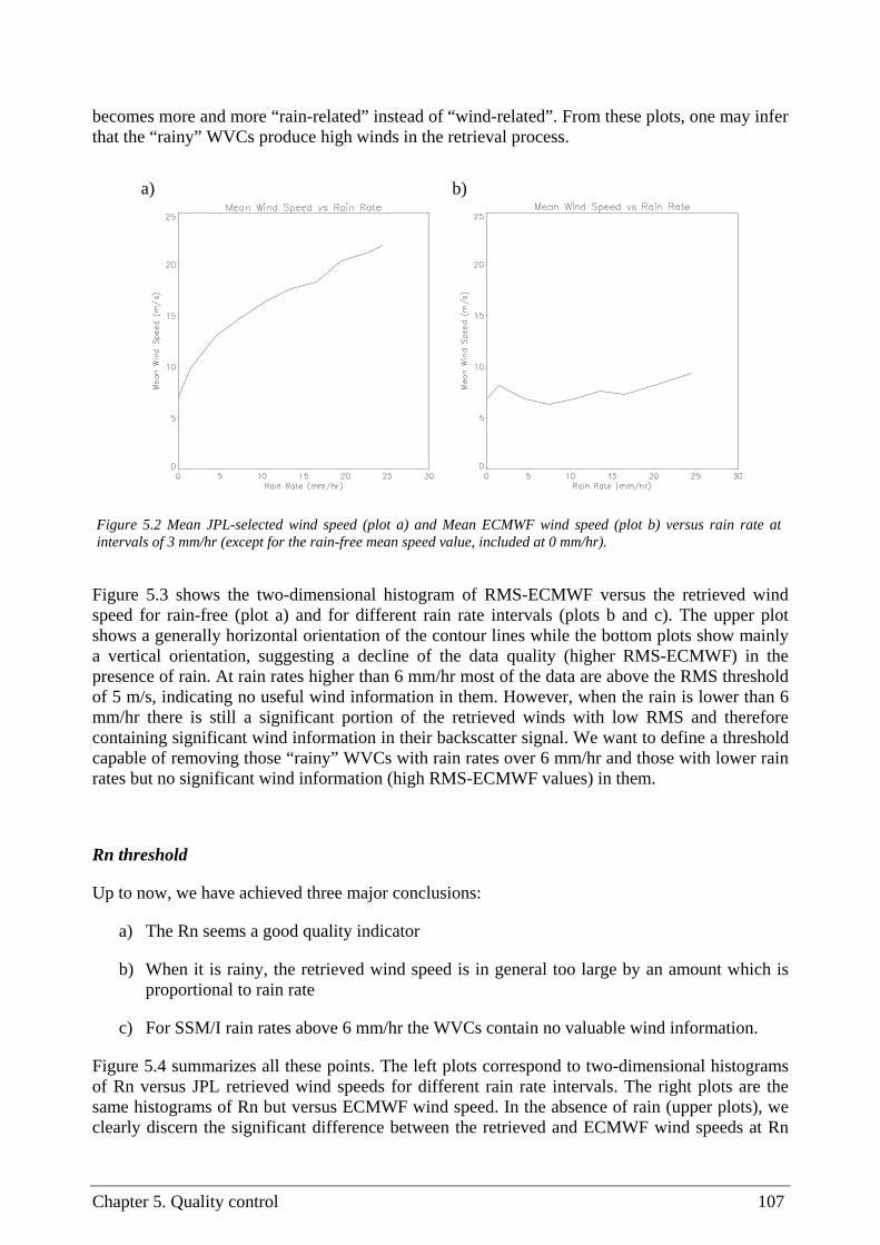
Chapter 5. Quality control 107
becomes more and more “rain-related” instead of “wind-related”. From these plots, one may infer that the “rainy” WVCs produce high winds in the retrieval process.
Figure 5.3 shows the two-dimensional histogram of RMS-ECMWF versus the retrieved wind speed for rain-free (plot a) and for different rain rate intervals (plots b and c). The upper plot shows a generally horizontal orientation of the contour lines while the bottom plots show mainly a vertical orientation, suggesting a decline of the data quality (higher RMS-ECMWF) in the presence of rain. At rain rates higher than 6 mm/hr most of the data are above the RMS threshold of 5 m/s, indicating no useful wind information in them. However, when the rain is lower than 6 mm/hr there is still a significant portion of the retrieved winds with low RMS and therefore containing significant wind information in their backscatter signal. We want to define a threshold capable of removing those “rainy” WVCs with rain rates over 6 mm/hr and those with lower rain rates but no significant wind information (high RMS-ECMWF values) in them.
Rn threshold
Up to now, we have achieved three major conclusions:
a) The Rn seems a good quality indicator
b) When it is rainy, the retrieved wind speed is in general too large by an amount which is proportional to rain rate
c) For SSM/I rain rates above 6 mm/hr the WVCs contain no valuable wind information.
Figure 5.4 summarizes all these points. The left plots correspond to two-dimensional histograms of Rn versus JPL retrieved wind speeds for different rain rate intervals. The right plots are the same histograms of Rn but versus ECMWF wind speed. In the absence of rain (upper plots), we clearly discern the significant difference between the retrieved and ECMWF wind speeds at Rn
a) b)
Figure 5.2 Mean JPL-selected wind speed (plot a) and Mean ECMWF wind speed (plot b) versus rain rate at intervals of 3 mm/hr (except for the rain-free mean speed value, included at 0 mm/hr).

108 Wind field retrieval from satellite radar systems
values larger than 4 (see speed shift in the contour line), denoting a poor quality of the retrieved solutions. Thus, in case of no rain, high Rn is seemingly associated with systematically wrong winds. This wind speed difference at Rn values larger than 4 becomes significantly larger (2-3 m/s) in the middle plots while for low Rn (darkest contour) there is no significant difference. This is denoting that although at mid and high winds the wind retrieval is not very much affected by low rain rates, at low winds the sensitivity to rain is so important that even at low rain rates the quality of the retrievals is poor. This is an expected result as for low winds you get lower backscatter than for high winds and therefore the backscattering from the rain droplets becomes more significant. Comparing the contours from the left and the right plots, there is a positive shift of the left ones with respect to the right ones (indicating a positive bias of the retrieved speeds with respect to ECMWF speeds) as the rain rate increases. This shift becomes excessively large and unacceptable (more than 10 m/s) for rain rates over 6 mm/hr (bottom plots), denoting again the poor quality of the retrieved solutions.
a)
b) c)
Figure 5.3 Two-dimensional histograms of RMS-ECMWF versus JPL-selected wind speed for rain-free (plot a), for rain rates from 0 to 6 mm/hr (plot b) and for rain rates above 6 mm/hr (plot c). The contouring is the same as in Figure 5.1.
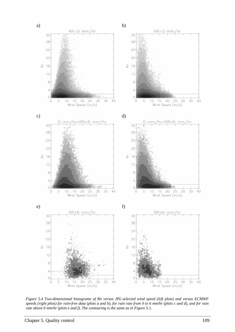
Chapter 5. Quality control 109
a) b)
c) d)
e) f)
Figure 5.4 Two-dimensional histograms of Rn versus JPL-selected wind speed (left plots) and versus ECMWF speeds (right plots) for rain-free data (plots a and b), for rain rate from 0 to 6 mm/hr (plots c and d), and for rain rate above 6 mm/hr (plots e and f). The contouring is the same as in Figure 5.1.

110 Wind field retrieval from satellite radar systems
In the definition of a Rn threshold we would like to achieve the following goals:
• Maximum poor-quality data rejection, including rain;
• Minimum good-quality data rejection.
As said before, the Rn threshold may be dependent on the retrieved wind speed. Figures 5.4a and 5.4b (no rain) suggest that the threshold should include and follow the contour lines that are very similar in both plots (showing good-quality data). Obviously, this threshold should become constant at a certain wind speed. Otherwise, we would start rejecting more and more data for increasing wind speed, until the threshold reaches zero at a certain wind speed from where on all higher retrieved speeds would be rejected. Figures 5.4a and 5.4b do not suggest poor quality of all high wind speeds. The constant threshold value has to be a compromise between the amount of high-wind data we want to keep and the amount of “rainy” data we want to reject.
From Figure 5.1, it is obvious that for higher winds we should be more critical with the Rn threshold. Therefore and in order to reject most of the “rainy” data (see Figure 5.4e), we define a minimum threshold value of 2 for speeds higher than 15 m/s. From Figures 5.4a and 5.4b, we define a parabolic threshold with a maximum value of 4 at 5 m/s, which reaches a value of 2 at 15 m/s (see the Rn threshold in black solid lines in Figure 5.4). Therefore, the defined threshold function is:
,5,100
2,4
,
2/15
)(/15
00
200
=−==
=⇒>−⋅+=⇒≤
vAy
where
ysmv
vvAyysmv
(5.1)
v is the retrieved (JPL-selected) wind speed and y the Rn threshold value.
Note that we have tested different thresholds including: 1) different parabolas with maxima and minima at different Rn / Speed locations; 2) a constant value for all wind speeds; and 3) a constant value for all speeds but with a step (change in value) at different wind speed locations. None of them have given better results than the one defined above according to our statistics and the two previously mentioned goals. Although the validation procedure has been used for threshold testing and tuning purposes, in the next section, we do only present the threshold with best validation results, i.e., the above defined threshold (see equation 5.1).
5.1.3 Threshold validation
We test the defined threshold against the set of ECMWF and SSM/I collocations (see section 5.1.1). [Note: we have performed the same validation with a different set of data and got the same results]. The test consists of looking at the Rn of the JPL-selected solution of any WVC. If the Rn is lower or equal to the threshold, the WVC is accepted; otherwise, the WVC is rejected. The results for the sweet parts of the swath are shown in tables 5.1, 5.2 and 5.3.

Chapter 5. Quality control 111
Table 5.1 shows the percentage of accepted and rejected WVCs from all the WVCs, segregated by wind speed intervals. 5.6% of data are rejected and the rejection rate is increasing with wind speed. This is an expected result. As “rainy” cells result in higher retrieved wind speeds (the larger the rain rate the larger the speed bias) and we want to get rid of those cells, the amount of rejections should increase with wind speed. However, in order to reject rain, we have defined a threshold that decreases with wind speed (up to 15 m/s where it remains constant) and therefore we might reject an increasing amount of “good” solutions as well.
Table 5.2 shows the total and the percentage of the accepted and rejected solutions for above and below a RMS-ECMWF threshold of 5 m/s. For the total, accepted and rejected classes, the different RMS-ECMWF value is also shown. On the one hand, there is a very small portion of rejected data (2.9 %) with RMS values below 5 m/s, indicating that most of the “good” quality solutions have been accepted. On the other hand, there is a significant percentage of rejected data (35.2%) with RMS values over 5 m/s, showing that the Rn threshold is effective in rejecting poor-quality data. The difference between the mean RMS of rejected and accepted data is 4 m/s, showing again the effectiveness of the Rn threshold.
Table 5.3 shows the percentage of the accepted and rejected solutions divided by rain rate intervals. When there is no rain, the percentage of rejections is 3.4%. If we compare this result with the total portion of rejections given in table 5.1 (5.6%) we can conclude that in more than 2% of the cases we are rejecting “rainy” cells. When the rain is over 6 mm/hr, most of the “rainy” cells are rejected (87.3%), denoting a very good behaviour of the Rn threshold. When the rain is lower or equal to 6 mm/hr, the percentage of rejections decrease significantly (29.4%) compared to higher rain rates. As said in the previous section, at these rain rates we are still getting “fair” quality winds (with enough wind information) that we may want to keep, but still there is a significant portion of low winds (see discussion of Figure 5.4) of poor quality that are rejected. In this sense, we achieve a good compromise in the screening of cases in the absence of rain (3.4% of rejections) and in cases of SSM/I rain over 6 mm/hr (87.3% of rejections).
Figure 5.5 shows the two-dimensional histograms of RMS-ECMWF versus retrieved wind speed for different rain intervals. The left plots correspond to the accepted solutions and the right plots to the rejected solutions. It is clear when comparing the contour lines of the left with the right plots that the latter show a much more vertical orientation with the maximum (darkest contour) significantly higher than the former (accepted solutions). This is a way to show the mean RMS difference between the accepted and the rejected solutions presented in table 5.2. For rain rates over 6 mm/hr (see bottom plots) most of the solutions are rejected.
Comparing the distributions of Figures 5.3a and 5.3b (prior to QC) with the distributions of Figures 5.5a and 5.5c (accepted solutions), it is discernible that either for no rain or for rain rate lower than 6 mm/hr, the distributions have become flatter (less vertically oriented) after QC. This indicates a general decrease of the mean RMS and therefore a good performance of the method.
Tables 5.4, 5.5 and 5.6 are the same as tables 5.1, 5.2 and 5.3 but for the nadir swath. As discussed in section 2.2.2, in the nadir swath, there is not enough azimuth diversity in the σº views and the inversion skill is significantly lower compared to the sweet regions, where there is good azimuth diversity. In other words, the MLE wind-information content is not so meaningful in the nadir swath as it is in the sweet swath. This will in turn affect the skill of the QC procedure, being lower in the nadir than in the sweet regions. And this is what we see in the results shown in the tables mentioned above.

112 Wind field retrieval from satellite radar systems
Table 5.1 Accepted and rejected WVCs from all the WVCs (sweet swath).
Total V<10 10≤V≤15 V>15
Num. Points (n/a) 4826841 3796408 859747 170686
Accepted (%) 94.4 95.8 91 81
Rejected (%) 5.6 4.2 9 19
Table 5.2 Relative quality of accepted and rejected WVCs (sweet swath).
RMS≤5 RMS>5 Mean RMS (m/s)
Total (n/a) 4429905 396970 2.46
Accepted (%) 97.1 64.8 2.24
Rejected (%) 2.9 35.2 6.24
Table 5.3 Accepted and rejected WVCs by rain rate intervals (sweet swath).
RR=0 0<RR≤6 RR>6
Num. Points (n/a) 1027124 88311 3664
Accepted (%) 96.6 70.6 12.7
Rejected (%) 3.4 29.4 87.3
Table 5.4 Accepted and rejected WVCs from all the WVCs (nadir swath).
Total V<10 10≤V≤15 V>15
Num. Points (n/a) 2812095 2186477 511131 114487
Accepted (%) 93.7 95.9 88.5 76.2
Rejected (%) 6.3 4.1 11.5 23.8
Table 5.5 Relative quality of accepted and rejected WVCs (nadir swath).
RMS≤5 RMS>5 Mean RMS (m/s)
Total (n/a) 2483112 329113 2.81
Accepted (%) 96.8 70.6 2.55
Rejected (%) 3.2 29.4 6.62
Table 5.6 Accepted and rejected WVCs by rain rate intervals (nadir swath).
RR=0 0<RR≤6 RR>6
Num. Points (n/a) 572894 47529 2526
Accepted (%) 96 64.5 14.8
Rejected (%) 4 35.5 85.2
Note: RMS is referred as the mean RMS of vector difference between JPL-retrieved winds and ECMWF winds in m/s; V is the JPL-selected wind speed in m/s; and RR is the SSM/I rain rate in mm/hr.

Chapter 5. Quality control 113
a) b)
c) d)
e) f)
Figure 5.5 Two-dimensional histograms of RMS-ECMWF versus JPL-selected wind speed for the accepted (left plots) and rejected WVCs (right plots). The top plots correspond to rain-free data, the middle plots to rain rate from 0 to 6 mm/hr and the bottom plots to rain rate above 6 mm/hr. The contouring is the same as in Figure 5.1.

114 Wind field retrieval from satellite radar systems
Comparing table 5.4 with table 5.1, we see a larger percentage of rejections in the nadir swath, which increases with wind speed. At speeds higher than 15 m/s, 23.8% of the data are rejected. This represents almost 5% more rejections than in the sweet regions.
Comparing table 5.5 with table 5.2, there is a slightly larger percentage of rejections at RMS-ECMWF ≤ 5m/s and a smaller percentage of rejections at RMS-ECMWF > 5m/s in the nadir swath, indicating a slight decrease in the performance of the QC procedure. Although the RMS-ECMWF of the accepted solutions is slightly higher in the nadir swath, the RMS-ECMWF difference between accepted and rejected solutions is the same (4 m/s), showing a comparable result in both regions.
Comparing table 5.6 with table 5.3, when rain is over 6 mm/hr there are slightly less rejections in the nadir swath. This shows again a slightly worse performance in the nadir swath, especially if we consider that, overall (see tables 5.1 and 5.4), this region suffers more rejections (especially at high winds, where the rain is “located”). However, the percentage of rejections for rain under 6 mm/hr is about 6% higher in the nadir swath. Most of these rejections have an RMS-ECMWF over 5 m/s. This result is unexpectedly positive, as even if the overall portion of rejections with RMS-ECMWF > 5 m/s (see tables 5.2 and 5.5) is about 6% smaller in the nadir swath, the portion of rejections when the rain is below 6 mm/hr is around 6% higher for the nadir swath.
In general, the skill of the QC procedure is good in both regions of the swath, although it is slightly better in the sweet region.
The QC procedure presented in here is based on the selected solution information. We have also tested a QC based on the first rank solution information, i.e., using both the 1st rank MLE value and the <MLE> computed from the 1st rank solution in equation 2.10, as well as a Rn threshold based on the 1st rank wind speed. It shows similar results to the QC based on the selected solution, although the latter is marginally better. A possible explanation for this small difference is that there is more correlation between a geophysical disturbance and the MLE of the selected solution rather than with the MLE of the first-rank solution. In other words, there is some correlation between the data quality and the number of the wind solutions and their corresponding MLE values. Ambiguity removal then picks the geophysically most consistent solution. Therefore, we recommend the use of the QC based on the selected solution.
5.1.4 Cases
In this section, we show a few wind field examples where the QC procedure has been applied. Figures 5.6, 5.7 and 5.8 show triple collocated QuikSCAT-ECMWF-SSM/I data. The arrows in Figures 5.6a, 5.7a, and 5.8a correspond to the QuikSCAT JPL-selected wind solutions and the greyscales represent the accepted (grey) and the rejected (black) solutions by the Rn threshold (QC). The squares correspond to the collocated SSM/I rain data, where the size of the squares annotates rain rate. The arrows in Figures 5.6b, 5.7b, and 5.8b correspond to the collocated ECMWF winds. The solid lines divide the different regions of the swath (outer, sweet and nadir).
In Figure 5.6, there is a case of significant rain (up to 25 mm/hr) over the entire plot, especially in the middle-left and upper-right parts. It is clearly discernible that most of the areas with rain rate above 6 mm/hr (mid-large squares) are rejected by the QC.

Chapter 5. Quality control 115
At about 12º latitude, there is a “band” of rejections going from the centre to the right side of the plot. This area is dividing a mid and high wind speed area (south part) from a low speed one (north part), suggesting the presence of a wind front. The QC is performing well as in the frontal area, confused sea state is expected (due to high temporal wind variability) and therefore poor-quality wind solutions exist. The wind field in Figure 5.6b (ECMWF wind field) does not at all reflect the spatial detail seen in Figure 5.6a, showing a potential positive impact of assimilation of QuikSCAT winds into the ECMWF model.
Although the low wind speed region shows some erratic flow patterns, most of the wind solutions have been accepted by the QC. This region is mostly located in the nadir part of the swath. As said before, in the nadir regions there is a lack of azimuth diversity in the σº views. As discussed in chapters 2 and 3, this affects the skill of the inversion and in turn the skill of the standard wind retrieval, in particular at low wind speeds where the GMF is less sensitive to wind direction changes. Our QC will not detect these points since they do not exhibit large Rn. However, an improved wind retrieval scheme, as shown in chapter 3, will produce solution patterns that are more consistent.
CASE : 02/09/99 1400 UTC a) b)
Figure 5.6 Collocated QuikSCAT-ECMWF-SSM/I data. Plot a shows QuikSCAT wind field (JPL-selected winds), where grey corresponds to accepted WVCs and black to rejected WVCs. The size of the squares represent the different rain rates from 0 mm/hr (no square) to 25 mm/hr (the largest ones). Plot b shows the collocated ECMWF winds. The solid lines separate different regions of the swath. In this case, the left side of the plot corresponds to the sweet-left region, the middle to the nadir region and the right side to the sweet-right region. The acquisition date was September 2 1999 at 14 hours UTC.

116 Wind field retrieval from satellite radar systems
In Figure 5.7a, the presence of a wind front is clearly discernible in the middle of the plot, where again a confused sea state and therefore poor-quality winds are expected. WVCs along the front line are rejected by QC. This is also the case for the centre of the low at the bottom of the plot, where there is probably extreme temporal and spatial sea state variability or rain. At the left side of the wind front we see a region of significant rain (above 6 mm/hr), which has been successfully detected by the QC.
CASE : 28/08/99 0500 UTC a) b)
Figure 5.7 Same as Figure 5.6 but for different date (August 28 1999 at 5 hours UTC) and location. The solid lines separate the nadir (left side), the sweet-left (middle) and the outer-left (right side) regions.
Although the QC is not expected to work fine in the outer regions (see discussion at the beginning of this chapter), the same procedure (including the threshold defined in section 5.1.2) is also applied in such regions in this section. As it is discernible in Figure 5.7a, there are very few rejections in the outer region (right side of the plot). This is an expected result (see QC discussion in section 6.2.1). In general, the QC does not detect much of the poor-quality data in the outer regions. However, in this case, the flow looks consistent and therefore the QC apparently seems to work.
The ECMWF forecast (Figure 5.7b) does not accurately place the centre of the low and the associated wind front is not so pronounced as in the QuikSCAT plot (Figure 5.7a). This example illustrates again the potential positive impact of assimilating QuikSCAT winds into ECMWF after using our QC.
Figure 5.8 shows a clear pure wind case. No fronts were predicted by ECMWF (plot b) and almost no rain was observed by SSM/I. Most of the wind solutions have been accepted by the
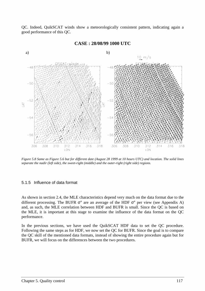
Chapter 5. Quality control 117
QC. Indeed, QuikSCAT winds show a meteorologically consistent pattern, indicating again a good performance of this QC.
CASE : 28/08/99 1000 UTC a) b)
Figure 5.8 Same as Figure 5.6 but for different date (August 28 1999 at 10 hours UTC) and location. The solid lines separate the nadir (left side), the sweet-right (middle) and the outer-right (right side) regions.
5.1.5 Influence of data format
As shown in section 2.4, the MLE characteristics depend very much on the data format due to the different processing. The BUFR σ° are an average of the HDF σ° per view (see Appendix A) and, as such, the MLE correlation between HDF and BUFR is small. Since the QC is based on the MLE, it is important at this stage to examine the influence of the data format on the QC performance.
In the previous sections, we have used the QuikSCAT HDF data to set the QC procedure. Following the same steps as for HDF, we now set the QC for BUFR. Since the goal is to compare the QC skill of the mentioned data formats, instead of showing the entire procedure again but for BUFR, we will focus on the differences between the two procedures.
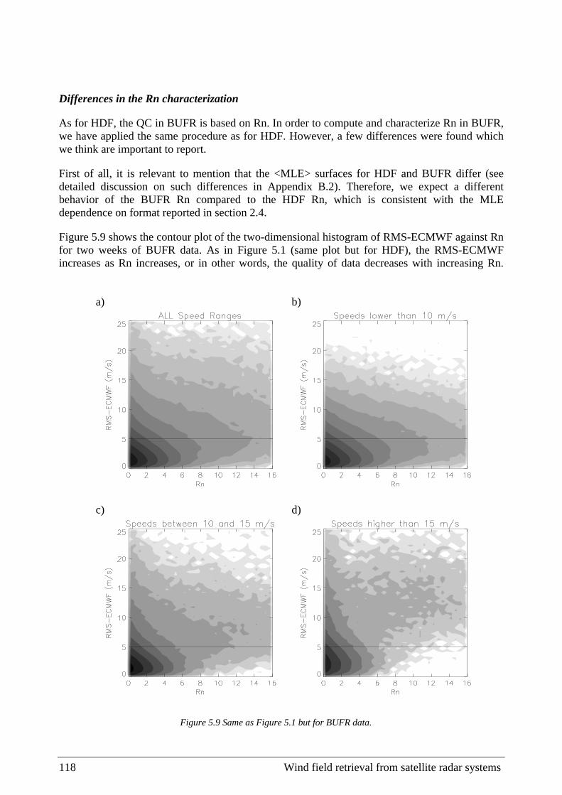
118 Wind field retrieval from satellite radar systems
Differences in the Rn characterization
As for HDF, the QC in BUFR is based on Rn. In order to compute and characterize Rn in BUFR, we have applied the same procedure as for HDF. However, a few differences were found which we think are important to report.
First of all, it is relevant to mention that the <MLE> surfaces for HDF and BUFR differ (see detailed discussion on such differences in Appendix B.2). Therefore, we expect a different behavior of the BUFR Rn compared to the HDF Rn, which is consistent with the MLE dependence on format reported in section 2.4.
Figure 5.9 shows the contour plot of the two-dimensional histogram of RMS-ECMWF against Rn for two weeks of BUFR data. As in Figure 5.1 (same plot but for HDF), the RMS-ECMWF increases as Rn increases, or in other words, the quality of data decreases with increasing Rn.
a) b)
c) d)
Figure 5.9 Same as Figure 5.1 but for BUFR data.
Chapter 5. Quality control 119
From Figure 5.9b, 5.9c, and 5.9d we can also infer that the RMS-ECMWF is increasing more rapidly with Rn at higher wind speeds. However, when comparing Figures 5.1 and 5.9, it is clearly discernible that the RMS-ECMWF in HDF increases more rapidly with respect to Rn for all wind speeds, suggesting a better behaviour of the HDF Rn as a quality control indicator.
Nevertheless, we have looked at the same plots as in Figures 5.2 and 5.3 but for BUFR (not shown) and they are very similar to HDF. Therefore, the rain rate also proportionally increases the retrieved wind speed and, above 6 mm/hr, produces undesirable “rainy” WVCs. Moreover, the same plot as in Figure 5.4 but for BUFR (not shown) is very similar to HDF, suggesting that the optimal BUFR Rn threshold may be the same as that used for HDF. We therefore test equation 5.1 for BUFR.
Differences in the threshold validation
In the same way as in HDF (see section 5.1.3), we test the defined threshold against ECMWF and SSM/I collocations. The results for the sweet parts of the swath are shown in tables 5.7, 5.8 and 5.9, and the results for the nadir parts are shown in tables 5.10, 5.11 and 5.12. Tables 5.7-5.12 are equivalent to tables 5.1-5.6 (see section 5.1.3), respectively, but for BUFR data.
In general, the results show that the BUFR QC is slightly more critical than the HDF QC. This is consistent with the previous discussion on the Rn behaviour.
Comparing table 5.7 with table 5.1, we note a larger percentage of rejections in BUFR than in HDF at all speeds. From tables 5.8 and 5.2, we see that the RMS-ECMWF difference between accepted and rejected solutions is 4 m/s in HDF, while in BUFR is slightly lower than 3 m/s. However, this does not indicate a clear better performance of the HDF QC compared to BUFR, since overall RMS-ECMWF is lower for BUFR (2.26 m/s) than for HDF (2.46 m/s)1. From tables 5.9 and 5.3, the amount of “rainy” WVCs rejected is slightly lower for BUFR, perhaps as a result of the slightly poorer performance of the BUFR QC compared to the HDF QC2. Overall, the results show that HDF and BUFR QC are of comparable performance.
Comparing the BUFR QC (tables 5.10-5.12) with the HDF QC (tables 5.4-5.6) in the nadir region, we can draw similar conclusions than for the sweet parts of the swath, except that, in this case, the total number of rejections in BUFR is comparable to HDF. The reason why the number of rejections in the nadir swath is not higher for BUFR is that the <MLE> in BUFR is misfit towards higher values (compared to the filtered mean MLE values) in the nadir parts (see discussion of Figure B.2 in Appendix B.2). This in turn decreases the value of Rn and therefore decreases the number of rejections.
In general, the BUFR QC works fine and is comparable to the HDF QC. Therefore, the properties of the MLE as a QC indicator, i.e., the MLE information content, are almost independent of the data format used, despite the important differences between the MLE distributions, e.g., small correlation between HDF and BUFR, as discussed in section 2.4. In other words, anomalies like
1 The selected solution in the BUFR product is replaced by the DIR solution (see section 3.2). Since DIR is oversmoothing the retrieved field, the BUFR selected field is expected to be more in agreement with ECMWF than HDF. 2 It seems like a Rn threshold for BUFR that produces the same rejection rate as for HDF (i.e., 5.6%) would give better scores. This has not been tested.

120 Wind field retrieval from satellite radar systems
Table 5.7 Accepted and rejected WVCs from all the WVCs (sweet swath).
Total V<10 10≤V≤15 V>15
Num. Points (n/a) 3005557 2261475 617140 126942
Accepted (%) 93.3 94.9 90.5 79.2
Rejected (%) 6.7 5.1 9.5 20.8
Table 5.8 Relative quality of accepted and rejected WVCs (sweet swath).
RMS≤5 RMS>5 Mean RMS (m/s)
Total (n/a) 2805852 203084 2.26
Accepted (%) 95.5 63.8 2.07
Rejected (%) 4.5 36.2 4.92
Table 5.9 Accepted and rejected WVCs by rain rate intervals (sweet swath).
RR=0 0<RR≤6 RR>6
Num. Points (n/a) 647292 56939 2904
Accepted (%) 95.3 72.7 16.1
Rejected (%) 4.7 27.3 83.9
Table 5.10 Accepted and rejected WVCs from all the WVCs (nadir swath).
Total V<10 10≤V≤15 V>15
Num. Points (n/a) 1744647 1290254 372353 82040
Accepted (%) 93.9 95.9 90.3 79.1
Rejected (%) 6.1 4.1 9.7 20.9
Table 5.11 Relative quality of accepted and rejected WVCs (nadir swath).
RMS≤5 RMS>5 Mean RMS (m/s)
Total (n/a) 1585453 160703 2.48
Accepted (%) 96.1 72.3 2.29
Rejected (%) 3.9 27.7 5.49
Table 5.12 Accepted and rejected WVCs by rain rate intervals (nadir swath).
RR=0 0<RR≤6 RR>6
Num. Points (n/a) 360953 28150 1536
Accepted (%) 95.9 70.7 19.4
Rejected (%) 4.1 29.3 80.6
Note: RMS is referred as the mean RMS of vector difference between JPL-retrieved winds and ECMWF winds in m/s; V is the JPL-selected wind speed in m/s; and RR is the SSM/I rain rate in mm/hr.
Chapter 5. Quality control 121
rain cause similar effects in both HDF and BUFR σ° products, that is, HDF and BUFR MLEs are strongly correlated in such cases.
5.2 KNMI quality control versus JPL rain flag
In the presence of extreme weather events, the likelihood of rain is relatively high and the QC of SeaWinds particularly important, according to the KNMI experience with NRT processing of SeaWinds data (http://www.knmi.nl/scatterometer). Although the KNMI QC is effective in rejecting rain-contaminated data, additional information on rain may be needed. In this respect, since May 2000, the SeaWinds data products, including the NRT data distributed by the National Oceanic and Atmospheric Administration (NOAA), have a rain flag (JPL, 2001). Since both the KNMI QC and the JPL rain flag are used in NRT processing, it is useful to compare them in order to improve the quality control for SeaWinds. In this section, we test the JPL rain flag against our QC.
Also since May 2000, JPL wind retrievals have been produced using a new GMF called QSCAT-1 (see Appendix C). In order to perform a consistent comparison with the JPL rain flag (set simultaneously to QSCAT-1 GMF), the new data should be used. Therefore, the QC performed in section 5.1 needs to be revised for the new data. This is done in Appendix D. In summary, the MLE characteristics do not significantly change and it is therefore concluded that the same QC procedure (i.e., same <MLE> surface and Rn threshold) can be used with the new QuikSCAT data (produced with the QSCAT-1 GMF).
5.2.1 JPL rain flag description
In January 2000, JPL incorporated in the QuikSCAT products two different rain flags based on the mp_rain_probability and the nof_rain_index respectively. However, since May 2000, JPL merged both techniques into a single rain flag. This rain flag procedure is actually based on the mp_rain_probability and called the MUDH (Multidimensional Histogram) rain algorithm (Huddleston and Stiles, 2000). The nof_rain_index (Mears et al., 2000) is incorporated as an additional parameter in the MUDH rain algorithm, but it is currently not being used (zero weight is assigned to this parameter) in the computation of the rain flag (JPL, 2001).
Briefly, mp_rain_probability is the probability of encountering a columnar rain rate that is greater than 2km*mm/hr. This probability value is read directly from a table based on several input parameters including average brightness temperature (both H-pol and V-pol), normalized inter-view σ° difference, wind speed, wind direction relative to along track, and a normalized MLE. The space spanned by these parameters can detect whether the set of σº values used in wind retrieval contain a noteworthy component created by some physical phenomenon other than wind over the ocean’s surface, assuming that the most likely phenomenon is rain.
The final rain flag deduced from the MUDH rain algorithm is also incorporated in the QuikSCAT products and can be found in the wvc_quality_flag variable.

122 Wind field retrieval from satellite radar systems
5.2.2 Comparison
The JPL rain flag separates “rain” (rain rate above 2km*mm/hr) from “no rain” (rain rate below 2km*mm/hr) cases and the KNMI QC separates cases of poor quality to be rejected (above Rn threshold) from those of good quality to be accepted (below Rn threshold).
Both the JPL rain flag and the KNMI QC are meant to separate the usable data from the non-usable data. Therefore, the user should use only “no rain” data according to JPL rain flag and reject the “rain” data. In the same way, the user should accept or reject data according to KNMI QC, and therefore a study of the difference in behaviour of both procedures is of interest.
In order to make a consistent comparison, we have processed two weeks of HDF data and classified the results in four different categories: A) “JPL Rain Flag - No Rain” and “KNMI QC - Accepted”; B) “JPL Rain Flag - Rain” and “KNMI QC - Accepted”; C) “JPL Rain Flag - No Rain” and “KNMI QC - Rejected”; and D) “JPL Rain Flag - Rain” and “KNMI QC - Rejected”. In line with the previous paragraph, categories A and D show similarities and categories B and C show discrepancies between the two procedures.
In tables 5.13-5.15, we present the results of collocating 2 weeks of QuikSCAT HDF data (sweet regions only) with ECMWF winds and SSM/I rain data. [Note: we have performed the same comparison in the nadir swath and got similar results]. In total, there are about 5.2 million collocations with ECMWF and 1.1 million collocations with SSM/I. We refer to rain data when SSM/I surface rain rate (RR) value is above 2 mm/hr, and to rain-free data when SSM/I surface rain rate value is below 2 mm/hr.
Table 5.13 shows, by category, the percentage of total data, the QuikSCAT mean speed, the ECMWF mean speed, the mean bias (QuikSCAT minus ECMWF wind speed), the mean RMS of wind vector difference (RMS-ECMWF), the percentage of data with rain (RR>2 mm/hr), and the percentage of all rain points (RR>2 mm/hr).
The results in table 5.13 show very good agreement between both procedures, as 94% of the data corresponds to categories A and D (91.1% in A and 2.9% in D). Moreover, category A shows good-quality (0.5 m/s bias and 2.2 m/s RMS) rain-free (only 0.1% of data a rain contaminated) data while category D shows very poor-quality (5.1 m/s bias and 8.2 m/s RMS) and rain-contaminated (31.9% of data are rain contaminated) data.
Categories B and C contain 6% of the data and correspond to the differences in behaviour of both procedures.
Comparing both categories in terms of SSM/I rain detection, category B contains 13.9% of all the rain data while category C only contains 2.4%. Therefore, the JPL rain flag is more efficient as rain detector since only 7.6% (5.2% in A and 2.4% in C) of all rain data is not rejected, while the KNMI QC accepts 19.1% (5.2% in A and 13.9% in B) of rain data.
In terms of quality of the data, both categories contain data of poor quality, with similar bias (2.4 m/s in B and 1.7 m/s in C) and RMS (4.8 m/s in B and 4.1 m/s in C) values. The KNMI QC is more efficient in rejecting poor-quality data than the JPL rain flag since category C contains

Chapter 5. Quality control 123
twice as much data as category B (4% in C; 2% in B). However, the JPL rain flag seems to work reasonably well as a QC flag as categories B and D show that only 27% of that data (13.6% in B and 31.9% in D) are rain contaminated data and therefore the rest are rain-free data but still of poor quality.
Tables 5.14 and 5.15 are similar to table 5.13 but only for rain-free data and rain data respectively. Table 5.14 contains about 1.1 million data and table 5.15 about 17000 data.
Table 5.14 shows very similar results to table 5.13. The most significant result is that for rain-free data, categories B and D contain poor-quality data, as seen from the high bias (2.2 m/s in B and 4.4 m/s in D) and RMS (4.4 m/s in B and 7 m/s in D). This confirms the JPL rain flag as a Quality Control flag as well.
Table 5.15 shows clearly the effect of rain in the quality of the data. All categories have larger bias and RMS values compared to tables 5.13 and 5.14. In particular, category A contains 5.2% of rainy data, which are clearly of poor quality (2.4 m/s bias and 5.5 m/s RMS). Neither the JPL rain flag nor the KNMI QC detects these data.
A B C D
Table 5.13 Comparison for all data.
JPL Rain Flag No Rain
JPL Rain Flag Rain
KNMI QC Accepted
Number of data (%): 91.1 QuikSCAT Mean Speed (m/s): 7.6 ECMWF Mean Speed (m/s): 7.1 Bias-ECMWF (m/s): 0.5 RMS-ECMWF (m/s): 2.2 Rain > 2 mm/hr (%1): 0.1 Rain > 2 mm/hr (%2): 5.2
Number of data (%): 2.0 QuikSCAT Mean Speed (m/s): 14.2 ECMWF Mean Speed (m/s): 11.8 Bias-ECMWF (m/s): 2.4 RMS-ECMWF (m/s): 4.8 Rain > 2 mm/hr (%1): 13.6 Rain > 2 mm/hr (%2): 13.9
KNMI QC Rejected
Number of data (%): 4.0 QuikSCAT Mean Speed (m/s): 9.1 ECMWF Mean Speed (m/s): 7.4 Bias-ECMWF (m/s): 1.7 RMS-ECMWF (m/s): 4.1 Rain > 2 mm/hr (%1): 1.0 Rain > 2 mm/hr (%2): 2.4
Number of data (%): 2.9 QuikSCAT Mean Speed (m/s): 12.3 ECMWF Mean Speed (m/s): 7.2 Bias-ECMWF (m/s): 5.1 RMS-ECMWF (m/s): 8.2 Rain > 2 mm/hr (%1): 31.9 Rain > 2 mm/hr (%2): 78.5
1 : % of data in this category with rain (RR> 2 mm/hr) 2 : % of all rain points (RR>2mm/hr)

124 Wind field retrieval from satellite radar systems
The results clearly show that the category B contains poor-quality data, including a significant amount of rainy data. Therefore, it seems a good idea to incorporate the JPL rain flag to the KNMI QC in order to improve the Quality Control of QuikSCAT data. However, according to the results in tables 5.13-5.15, the ECMWF wind speeds in category B are in general significantly higher (up to 4.7 m/s higher) than those in the other categories. This means that category B corresponds to dynamically active situations. Therefore, it could well be that this category systematically corresponds to frontal or low-pressure system areas where the discrepancy
A B C D
A B C D
Table 5.14 Comparison for rain-free data.
JPL Rain Flag No Rain
JPL Rain Flag Rain
KNMI QC Accepted
Number of data (%): 92.7 QuikSCAT Mean Speed (m/s): 7.0 ECMWF Mean Speed (m/s): 6.5 Bias-ECMWF (m/s): 0.5 RMS-ECMWF (m/s): 2.0
Number of data (%): 1.3 QuikSCAT Mean Speed (m/s): 12.2 ECMWF Mean Speed (m/s): 10.0 Bias-ECMWF (m/s): 2.2 RMS-ECMWF (m/s): 4.4
KNMI QC Rejected
Number of data (%): 3.5 QuikSCAT Mean Speed (m/s): 7.8 ECMWF Mean Speed (m/s): 5.9 Bias-ECMWF (m/s): 1.9 RMS-ECMWF (m/s): 4.2
Number of data (%): 2.5 QuikSCAT Mean Speed (m/s): 10.3 ECMWF Mean Speed (m/s): 5.9 Bias-ECMWF (m/s): 4.4 RMS-ECMWF (m/s): 7.0
Table 5.15 Comparison for rain data.
JPL Rain Flag No Rain
JPL Rain Flag Rain
KNMI QC Accepted
Number of data (%): 5.2 QuikSCAT Mean Speed (m/s): 10.8 ECMWF Mean Speed (m/s): 8.4 Bias-ECMWF (m/s): 2.4 RMS-ECMWF (m/s): 5.5
Number of data (%): 13.9 QuikSCAT Mean Speed (m/s): 13.7 ECMWF Mean Speed (m/s): 9.0 Bias-ECMWF (m/s): 4.7 RMS-ECMWF (m/s): 8.2
KNMI QC Rejected
Number of data (%): 2.4 QuikSCAT Mean Speed (m/s): 9.9 ECMWF Mean Speed (m/s): 6.6 Bias-ECMWF (m/s): 3.3 RMS-ECMWF (m/s): 6.1
Number of data (%): 78.5 QuikSCAT Mean Speed (m/s): 14.4 ECMWF Mean Speed (m/s): 6.4 Bias-ECMWF (m/s): 8.0 RMS-ECMWF (m/s): 11.2

Chapter 5. Quality control 125
between ECMWF and QuikSCAT is indeed of valuable interest, in which case, these data should be kept and not rejected.
In order to determine the convenience of incorporating the JPL rain flag in the KNMI QC, some meteorological cases need to be examined.
5.2.3 Cases
Many meteorological cases were examined. Indeed, some systematic effects were found that help in understanding the statistical results of section 5.2.2. In this section, we show two wind field examples, which are representative of the entire set of examined cases. Figures 5.10 and 5.11 show QuikSCAT winds where both the KNMI QC and the JPL rain flag have been applied. The arrows in Figures 5.10a and 5.11a correspond to the QuikSCAT JPL-selected wind solutions and the colors represent categories A (green), B (yellow), C (blue) and D (red). Figures 5.10b and 5.11b are the same as Figures 5.10a and 5.11a, respectively, but arrows belonging to categories C and D are substituted by dots.
In Figure 5.10, the presence of a low-pressure system in the western North-Atlantic Ocean is clearly discernible in the middle-right part of the plot. A wind front is partly visible going from northeast to south of the low. The KNMI QC has rejected data in the vicinity of the low and along the front line where a confused sea state is expected (see red and blue arrows). We can also see KNMI QC rejections at low-wind areas (blue arrows at bottom part of the plot), where the QuikSCAT retrieved wind flow is clearly inconsistent. As anticipated in the previous section, category B winds (yellow arrows) are mainly focused in the most dynamical area.
Looking at the same case but only showing category A and category B winds (accepted winds after KNMI QC most of the yellow arrows show a spatially consistent flow which should be kept. Moreover, the closest Meteosat image (not shown) to the QuikSCAT pass reveals no clouds (therefore no rain) south of the low (where most yellow arrows are located). We discern very few undesirable yellow arrows in the vicinity of the low (most likely poor-quality winds). Therefore, since the consistent category B winds (yellow) are located in the sweet part of the QuikSCAT swath, it seems that the KNMI QC works fine in these regions.
Figure 5.11 shows a front line in the middle of the plot associated with a low-pressure system, which is not observed by QuikSCAT, presumably located around 49° North and 314° East. The red arrows in the centre of Figure 5.11a clearly show the presence of rain bands along the front line. This is confirmed by SSM/I (not shown), which detected significant rain (rain rates above 6 mm/hr) in this area. As in the previous case, there is a large number of consistent winds rejected by the JPL rain flag (yellow arrows) in the sweet region (left side of the long black solid line). Some of these winds are rain-contaminated but the rain rate, according to SSM/I, is around 2 mm/hr. In section 5.1.2, we show no significant effect on the quality of high winds at these rain rates.
Looking at the same case but only for the accepted data after KNMI QC (Figure 5.11b), some inconsistent winds are still visible (yellow arrows), which are most likely rain contaminated (unfortunately no SSM/I observations available but Meteosat shows thick clouds over that area) and therefore undesirable. These arrows are located in the nadir region of the swath (between the black solid lines), where KNMI QC is expected to perform less well than in the sweet regions.
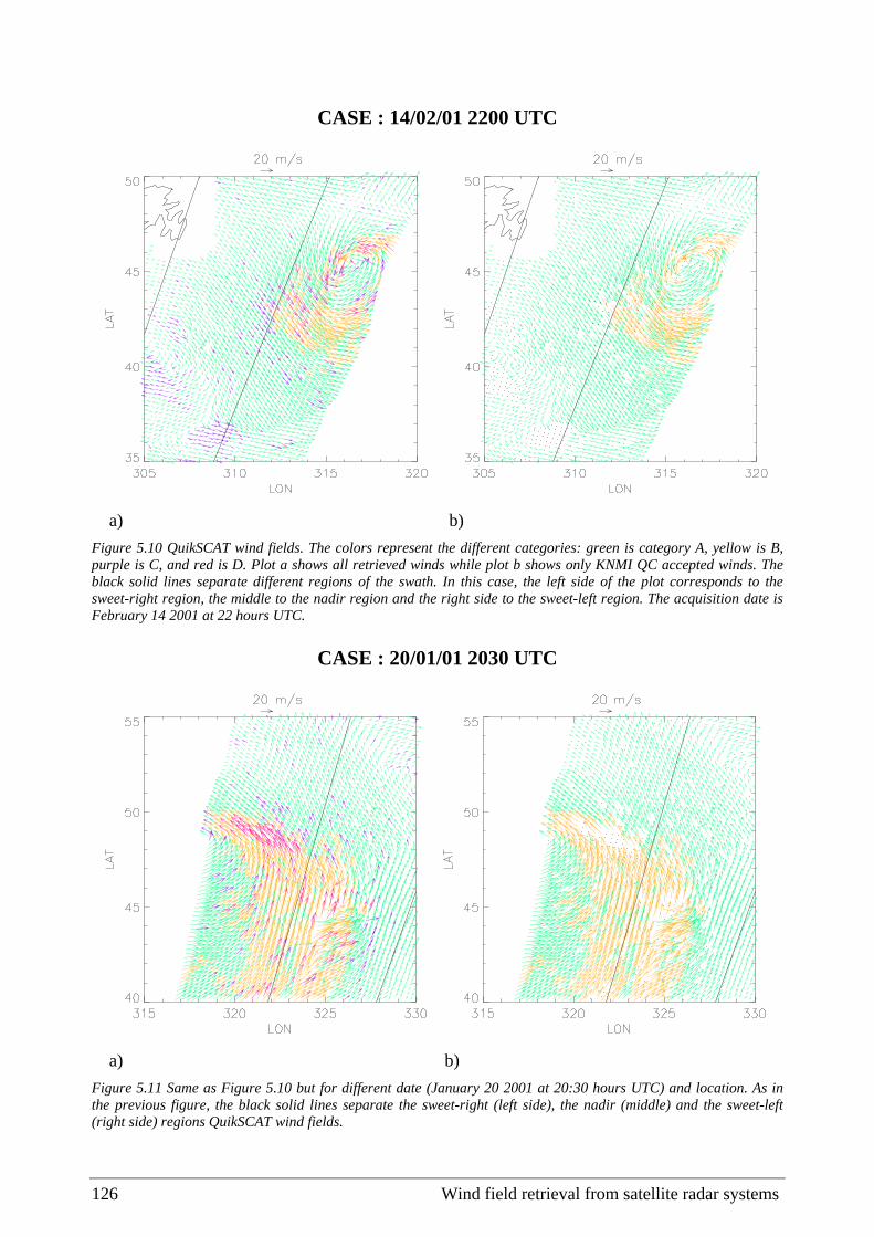
126 Wind field retrieval from satellite radar systems
CASE : 14/02/01 2200 UTC
a) b)
Figure 5.10 QuikSCAT wind fields. The colors represent the different categories: green is category A, yellow is B, purple is C, and red is D. Plot a shows all retrieved winds while plot b shows only KNMI QC accepted winds. The black solid lines separate different regions of the swath. In this case, the left side of the plot corresponds to the sweet-right region, the middle to the nadir region and the right side to the sweet-left region. The acquisition date is February 14 2001 at 22 hours UTC.
CASE : 20/01/01 2030 UTC
a) b)
Figure 5.11 Same as Figure 5.10 but for different date (January 20 2001 at 20:30 hours UTC) and location. As in the previous figure, the black solid lines separate the sweet-right (left side), the nadir (middle) and the sweet-left (right side) regions QuikSCAT wind fields.

Chapter 5. Quality control 127
As explained in section 5.1.3, the reason for the presence of inconsistent wind data lies in the nature of the QC. The QC is based on MLE and therefore on the quality of inversion. In contrast with the sweet regions, in the nadir region there is poor azimuth diversity among observations, which in turn leads to a decrease in the quality of inversion (see section 2.2.2). Subsequently, not only the KNMI QC but also the standard wind retrieval skills are lower in the nadir region than in the sweet regions of the swath. The lower quality of the standard retrievals is indicated in the right middle top part of Figure 5.11b, where several inconsistent winds, which are accepted by both KNMI QC and JPL rain flag (green arrows), are discernible (see chapter 3 for an improved wind retrieval scheme).
From the meteorological cases examined, we can conclude that category B winds are primarily located in dynamically active areas and in many cases they show very consistent wind flows, notably in the sweet swath. However, there are also several rain-contaminated cases and poor-quality winds in the nadir region, which belong to category B (and therefore not detected by KNMI QC) and are undesirable.
Figures 5.10b and 5.11b clearly show that rejecting category B winds can significantly reduce the synoptic-scale information content in some meteorological situations. Nevertheless, in the areas where the azimuth diversity is poor and therefore the quality of both the inversion and the KNMI QC is lower, the rejection of category B winds is necessary.
Therefore, for QuikSCAT QC purposes, we recommend the use of the KNMI QC in the sweet parts of the swath. In the nadir regions however, the combined use of the JPL rain flag and the KNMI QC procedure is recommended.
5.3 Conclusions
A MLE-based QC procedure, which follows the QC procedure investigated for NSCAT (Figa and Stoffelen, 2000) and the QC applied to the ERS scatterometer (Stoffelen, 1998a), is set in this chapter. In contrast with ERS scatterometer, NSCAT and SeaWinds are sensitive to volumetric rain absorption. As such, QC rejection for ERS is only activated in case of confused sea state, ice occurrence, etc, whereas in the case of QuikSCAT and NSCAT also rain is eliminated.
Collocations of QuikSCAT data with ECMWF winds and SSM/I rain were used to characterize and validate the QC (by Rn) for both the HDF and the BUFR formats. The empirically derived QC by Rn procedure proposed in this chapter, although applied for QuikSCAT data, is generic and, as such, can be applied to any overdetermined (i.e., three or more views) scatterometer system.
The results show a good correlation between the RMS-ECMWF (mean RMS of wind vector difference between ECMWF and QuikSCAT winds) and the Rn. The data quality, as measured by the inverse of RMS-ECMWF, decreases with increasing Rn, and the decrease rate becomes sharper for increasing retrieved wind speed (i.e., data quality becomes poor at medium Rn values when retrieved speeds are higher).

128 Wind field retrieval from satellite radar systems
The presence of rain artificially increases the retrieved winds, proportionally to the rain rate. For rain rates over 6 mm/hr, the backscatter measurements contain insufficient wind information but rather rain information, leading to poor-quality retrieved winds of typically 15-20 m/s.
We defined a Rn threshold dependent on wind speed, which is optimized to separate the good-quality cases from those of poor quality (including rain) in the inner swath (nodes 9 to 68). For HDF, the results show a RMS-ECMWF difference between accepted and rejected data of 4 m/s, most of the SSM/I “rainy” cells rejected, and more than 97% of good-quality data (low RMS-ECMWF) accepted.
The effectiveness of this QC procedure is illustrated with a few typical examples. Cases with meteorologically inconsistent spatial wind patterns are generally removed, while important information on the dynamical structures is kept. Patterns that are meteorologically consistent are kept in general.
The QC procedure works well in the entire inner swath although the skill in the sweet regions, where the MLE is most meaningful, is slightly better than in the nadir region. In terms of data format, the QC procedures in HDF and BUFR are of comparable skill, denoting that although the MLE characteristics change with the format, the MLE information content does not significantly change, as discussed in chapter 2.
A comprehensive comparison of our (KNMI) QC and the JPL rain flag is performed in order to determine an improved QC procedure for QuikSCAT. Again, the set of collocations with ECMWF winds and SSM/I rain data is used for this comparison. The KNMI QC detects 4% of poor-quality and almost rain-free data, which are not detected by the JPL rain flag. On the other hand, the JPL rain flag detects 2% of poor-quality and partially rain-contaminated data, which are not detected by the KNMI QC. The KNMI QC is more effective as QC indicator while the JPL rain flag is more effective as a rain detector.
The KNMI QC is based on the MLE parameter, which turns out to be a very good QC parameter. The JPL rain flag is based not only on the MLE but also on other parameters, which are identified to be sensitive to rain, such as the brightness temperature, the inter-view σ° difference, the wind direction and others. However, these parameters are not related to the quality of the data, which explains why the KNMI QC works better as quality indicator.
The results also show that the JPL rain flag tends to reject many data in rain-free dynamically active areas. We have illustrated this by two different meteorological cases. In both cases, there is an excess of consistent wind rejections by the JPL rain flag, especially in the sweet parts of the swath. In the nadir region, the inversion skill and consequently the KNMI QC efficiency are lower than those in the sweet regions due to the poor azimuth diversity. In this area the JPL rain flag is able to detect some flow-inconsistent and rain-contaminated winds, which are not detected by the KNMI QC.
For the QC of QuikSCAT data, we recommend the use of the KNMI QC. In the sweet swath, the KNMI QC suffices. However, the combination of the JPL rain flag and the KNMI QC is recommended in the nadir region.

Chapter 6. Discussion and outlook 129
Chapter 6
Discussion and Outlook
In this thesis, the wind field retrieval for satellite remote-sensing radar systems has been investigated, with special focus on two different systems: the QuikSCAT scatterometer and the ERS SAR. New methods have been proposed to improve the wind retrieval for both determined (especially, in areas with poor azimuth diversity) and underdetermined problems. Moreover, a generic MLE-based and empirically derived methodology is presented for QC purposes.
In the concluding sections of the previous chapters, many conclusions have been drawn together with several recommendations for future work. In the previous chapters, however, several aspects of the work presented in this thesis have been intentionally skipped or need some additional clarification. In this chapter, a brief and final discussion on some relevant aspects of this thesis together with a more general outlook is provided.
6.1 Wind retrieval
A general discussion on the wind retrieval procedures proposed in this thesis is presented in this section.
6.1.1 Multiple solution scheme versus general approach
The wind retrieval procedures proposed in chapters 3 and 4, i.e., the multiple solution scheme (MSS) and the general approach (GA), respectively, are conceptually very similar although they are presented in a different way. The GA (or more in particular, the SWRA) is related to the most general equation of the Bayesian approach (see section 2.1.1) and consists of minimizing a cost function with two terms: the observation and the background. The MSS uses a more constrained

130 Wind field retrieval from satellite radar systems
solution of the Bayesian approach, the MLE (see section 2.1.2), for inversion. However, for AR purposes, it uses a variational scheme, which consists of minimizing a cost function that includes the departures from the inverted solutions (i.e., observation term) and the departures from a NWP model (i.e., background term). Both wind retrieval procedures are therefore minimizing the same type of cost function.
Moreover, the MSS and the GA are flexible enough to accommodate different levels of determination of the problem, as shown in their corresponding cost functions. The MSS cost function uses a variable number of wind solutions according to the level of determination of the problem. That is, the more determined the problem (better azimuth diversity), the smaller the number of solutions in the observation term. Moreover, for each solution a probability of being the “true” wind is assigned and used in the cost function. Thus, the more determined the problem, the smaller the number of solutions with comparable probability. The MSS is therefore consistent with the level of determination of each WVC, allowing more influence of the background term as the problem becomes less determined, i.e., the larger the number of solutions with comparable probability in the observation term, the larger the overall weight of the background term in the cost function.
The mentioned flexibility is also present in the GA cost function. Now, the observation term allows large (infinite if you wish) numbers of solutions with equal probability (see isolines of Figure 4.3 in section 4.3.3.1), which will result in a larger influence of the background term in the cost function, as expected from an underdetermined system. However, the GA is flexible enough, such that it allows additional wind information to be included whenever it is available. For example, in the case of SAR, the wind direction information can sometimes be derived from the image (i.e., wind streaks) and, after a comprehensive characterization of the retrieval errors, it can be included in the observation term of the GA cost function, thus improving the retrievals.
Therefore, the MSS and the GA are complementary in that the former assumes that the problem is overdetermined but allows a decrease in the level of determination, as caused by the degradation of the azimuth diversity, i.e., as the QuikSCAT nadir is approached, and the latter assumes that the problem is underdetermined and allows an increase in the level of determination, as provided by the instrument capabilities, i.e., wind direction information derived from the SAR image pattern.
The main difference between the two procedures lies in the space of the observation term. The wind domain is used in the MSS, while the GA is using the backscatter domain. Stoffelen and Anderson (1997a) show that, for scatterometer data assimilation (similar to variational AR), it is better to use the wind domain in the observation term than the backscatter domain. The reason is that the uncertainty in the wind domain behaves in a Gaussian way and it is therefore easy to characterize the observation and background error, whereas in the backscatter domain, due to the highly non-linear transformation (GMF), the uncertainty or noise is more difficult to characterize. In the GA, however, the wind domain cannot be used because of the underdetermination problem. In other words, while the MLE inversion provides certain amount of wind solutions to the observation term of the MSS, no wind solutions can be provided to the same term of the GA (“standalone” inversion not possible because of underdetermination) and therefore backscatter information is used instead.
One could alternatively assume certain degree of determination in SAR and apply the MSS. The inversion of a single backscatter would produce a flat (null) MLE cost function, i.e., a large number of solutions (144, for a MLE cost function step size of 2.5°) with identical probability. These solutions, which lay on the solid line of Figure 1.8a, lay as well on the highest probability

Chapter 6. Discussion and outlook 131
ellipse (thick line) of Figure 4.3. In other words, if we only consider these wind solutions, the MSS and the GA are equivalent1. Strictly speaking, this alternative is not taking into account the underdetermination problem. However, it could well be that its implementation provides fair results. In such case, we could unify the satellite radar wind retrieval methods described in this thesis. It is therefore recommended to test the MSS for SAR wind retrieval.
6.1.2 QuikSCAT outer regions
In chapter 3, we revise the wind retrieval for determined problems and focus our work on the new challenges posed by the new instrument geometries, that is, on improving the wind retrieval over poor-azimuth diversity areas. The methodology proposed is actually implemented in the QuikSCAT inner swath and therefore valid for any overdetermined problem.
The QuikSCAT outer regions are characterized by an instrument geometry, which is similar to the Seasat SASS, i.e., two views. As discussed in section 1.4.1, for a two-view measurement system, i.e., case b, the wind retrieval problem is determined. Moreover, the wind accuracy of such systems is comparable to that of overdetermined systems with good azimuth diversity, e.g., QuikSCAT sweet regions, provided that there exists a good AR scheme that is able to cope with the large ambiguity problem of such systems (see section 2.2.2). As already mentioned, Stoffelen and Cats (1991) show the potential contribution of Seasat SASS winds in NWP data assimilation, and therefore the usefulness of two-view measurement systems.
The QuikSCAT outer region case differs somehow from the SASS case. The difference is in the azimuth diversity. While the SASS has an optimal azimuth separation, i.e., two views 90° apart (see sections 1.3.1 and 1.4.1), the azimuth separation for QuikSCAT monotonically decreases as we approach the edges of the outer swath (see Figure 1.9 in section 1.4.3). In chapter 3, we propose a method, the MSS, which allows a variable number of solutions from inversion, according to the level of determination or azimuth diversity, to be used for AR purposes. It seems reasonable to apply the same methodology (MSS) to the QuikSCAT outer regions. Moreover, the variational analysis AR used by the MSS should work significantly better for QuikSCAT than for SASS, since, in the case of QuikSCAT, the large (i.e., 1400-km wide) and almost unique wind information (i.e., low ambiguity) of the inner swath can be easily extrapolated to the few nodes of the outer regions, while for SASS, the ambiguity problem is over the entire swath, i.e., only two views available (see section 1.3.1).
Therefore, the methodology used in chapter 3 can also be applied to the QuikSCAT outer regions. However, as seen in chapter 2, the characteristics of the MLE change with the dimension of the measurement space. That is, the MLE distributions of two-view and four-view measurement systems differ. This means that the MSS is applicable to the QuikSCAT outer regions, provided that the solution probability is re-computed using the outer-swath MLE information and the observation term of the AR is tuned to the outer regions.
As discussed in section 1.4.3, the edges of the outer swath (nodes 1-2 and 75-76) are characterized by the presence of single-view measurements or by a very poor azimuth separation between the two views, i.e., equivalent to a single-view measurement. These areas present an
1 As for GA, a wind streak term could also be incorporated to the MSS cost function for SAR wind retrieval.

132 Wind field retrieval from satellite radar systems
underdetermination problem similar to the SAR and, as such, the methodology proposed in chapter 4 could be adapted for QuikSCAT and used in such areas for wind retrieval purposes. However, these areas (4 WVCs) represent a very small portion of the total QuikSCAT swath (76 WVCs) and the effort may not be worthwhile. At JPL, the wind retrieval is usually not performed in these WVCs.
It is important to say that, as shown in chapter 5, a comprehensive QC is needed to successfully derive winds from radar data. However, chapter 5 does only provide a QC procedure for overdetermined systems. The QC for single-view and two-view systems is addressed in section 6.2.
6.1.3 MLE norm
The MLE, as defined in equation 2.9 (see section 2.1.2), is usually computed with one of two different norms: a measurement error variance (Kp) proportional to the GMF simulated backscatter (σs°) or a Kp proportional to the backscatter measurement (σm°). As discussed in section 2.4.3, using a Kp proportional to σs° causes bias in the wind solutions (see Stoffelen and Anderson, 1997b). This is less true for a Kp proportional to σm° since the MLE norm remains fixed during the inversion process. However, there is no prior way to determine what is the best choice and usually tests are conducted for such purpose.
In this thesis, we use Kp proportional to σs° to compute the MLE at 25-km resolution since this is recommended/used by JPL (see equation 2.9) and part of the work described in this thesis uses the JPL inversion information (e.g., the QC work described in chapter 5 uses the JPL-selected MLE information). However, recent experiments seem to indicate that, for SeaWinds, a Kp proportional to σm° is slightly better than a Kp proportional to σs° at 100-km resolution (Portabella and Stoffelen, 2002). As such, the former is used in section 3.3.
A fixed norm has been successfully used to invert ERS winds (Stoffelen and Anderson, 1997c). The use of such MLE norm has not yet been tested for SeaWinds and is therefore recommended. Note that this is relevant for inversion but does not strongly impact QC, since the latter is based on a parameter which is supposed to remove the influence from the norm, that is, the normalized residual.
6.1.4 Data assimilation experience
In chapter 4, a wind retrieval method derived from the GA with a constrained set of assumptions, i.e., the SWRA is used to retrieve winds from SAR observations. A simplistic set of assumptions is used, notably no spatial correlation in the background errors. The latter is assumed to allow local minimization of the cost function, i.e., minimization in a WVC-by-WVC basis. However, as concluded in section 4.4, the wind retrieval may improve by implementing a background term where spatial correlation errors are included.
As discussed in section 6.1.1, there is a parallelism between the MSS and the GA. In particular, the background term is much the same although its implementation depends on the spatial

Chapter 6. Discussion and outlook 133
resolution of the observing system. The background term of the 2D-Var cost function (MSS) includes spatial error correlation information. The latter is derived from data assimilation schemes, such as 3D-Var or 4D-Var, and tuned for QuikSCAT AR purposes. The experience on data assimilation and the 2D-Var could be used to set a background term to the SWRA applicable for higher resolutions. In such case, additional effort would be required in the tuning, since the SWRA is used at a higher resolution (i.e., a few km) than the 2D-Var (i.e., 50-100 km).
6.2 Quality control
In this section, a general discussion on the QC for radar systems is presented, focusing on alternatives to the procedure proposed in chapter 5 for cases where the latter is not valid.
6.2.1 QuikSCAT outer regions
The MLE-based QC procedure (see section 5.1) is not effective for two-view measurement systems (case b of section 1.4.1), such as the Seasat SASS or the QuikSCAT outer regions. The MLE is used to invert two parameters, the wind speed and the wind direction. Therefore, the minimum number of independent views needed for wind retrieval is two (see section 1.4.1). As discussed at the beginning of chapter 5, in order to discriminate good-quality winds from poor-quality winds, the MLE has to be a good noise indicator. Thus, to use the MLE for QC, an additional backscatter view, i.e., at least three independent views, is needed to enable the retrieval of a third parameter, i.e., the noise. This is comprehensively illustrated in Figure 1.8 (see discussion on the effects of noise for a varying number of views in section 1.4.1).
However, the MLE-based procedure can be used in the outer regions as a first step to remove pairs of grossly inconsistent backscatter data. For such purpose, we can use the extrapolated <MLE> computed in section 2.3.1 to compute the Rn in the outer swath. As discussed in section 1.4.1, in such regions the wind vector is not overdetermined and generally multiple wind speed and direction combinations exist that exactly fit the measurements. Then the MLE is going to be zero or very close to zero in most of the cases, regardless of the quality of the data. Only for the exceptional case when the MLE is substantially larger than our extrapolated <MLE> we can infer that the data are of bad quality in these parts of the swath. This means that our QC procedure is going to be characterized by a small number of rejections in the outer regions. As such, our QC can be used to provide a gross check.
The limitations of a MLE-based QC can be inferred from Figure 2.3 (section 2.2.2). [Note: the MLE-based QC presented in chapter 5 has been applied in section 2.2.2; in the outer swath, the same QC as in the nadir swath, i.e., a combination of KNMI QC and JPL rain flag, is used]. Although the outer regions (bottom plots) show comparable accuracy to that of the sweet regions (top plots)1, the former shows a bias at high wind speeds (note how the contour lines are not
1 This is only true if we are able to successfully remove the large ambiguity in the outer swath (see discussion in sections 2.2.2 and 6.1.2).

134 Wind field retrieval from satellite radar systems
centered on the diagonal anymore), not present in the latter (compare Figures 2.3a and 2.3c), which denotes possibly rain contamination (see effects of rain on wind retrieval in section 5.1.2).
Additional efforts to QC the outer-region data can be done in the AR part of the wind retrieval procedure. As seen in chapter 3, the MSS uses a variational analysis AR, i.e., 2D-Var, which consists of minimizing a cost function with two terms, the observation and the background. Assuming that the background error information is a good reference, large discrepancies between the wind solutions provided by the MLE inversion and the analysis (i.e., output from variational AR) can be interpreted as poor-quality retrieved solutions. After a comprehensive validation, a threshold, which relates these discrepancies to the quality of the observations, can be set. This gross error check is the so-called variational QC.
A variational QC has not yet been tested. We anticipate that the wind vector consistency checks in the 2D-Var (i.e., variational QC) will be an effective complement for the MLE-based QC in the outer swath. Its development is therefore strongly recommended.
6.2.2 QuikSCAT low resolution
An important aspect of the 100-km product proposed in chapter 3, which needs to be examined, is the QC. Up to now, the 100-km product is using the MLE-based QC at 25-km resolution (see chapter 5) in the following way: if there is sufficient information on the 100-km WVC after QC (at least half of the 25-km WVCs within the 100-km WVC), the wind retrieval is performed.
The problem of using such QC procedure is illustrated in Figure 3.5 (section 3.2). Figure 3.5b shows the effects of using the recommended 25-km QC (see chapter 5), i.e., KNMI QC + JPL rain flag in the nadir and KNMI QC in sweet regions, in comparison with Figure 3.5a, where only the KNMI QC has been applied. On the one hand, as discussed in section 5.2.3, the JPL rain flag is rejecting a considerable amount of consistent winds, as seen in the Northern part (nadir region) of the wind flow (see WVCs with consistent wind solutions in Figure 3.5a removed in Figure 3.5b). On the other hand, the 25-km QC (using JPL rain flag) is able to reject several WVCs of poor quality, probably rain contaminated (see the nadir region WVCs with inconsistent solution pattern, both in speed and direction, in the lower half of Figure 3.5a, removed in Figure 3.5b). These poor-quality WVCs show zero probability in the direction of the flow (not shown) and therefore it is of great importance to identify these cases and reject them, regardless of the solution scheme, i.e., the standard procedure or the MSS (see chapter 3), we use. However, even if the 25-km QC is able to remove most of the poor-quality WVCs, a few of them still remain in Figure 3.5b (notice the absence of solutions aligned with the mean flow in a few nadir WVCs).
An alternative would be to use a variational QC (see section 6.2.1). This QC would reject large discrepancies with the control variable and, as such, many of the inconsistent nadir winds would be rejected. Moreover, in contrast with the JPL rain flag, it would generally keep the consistent wind flow. However, the rejection of discrepancies with the analysis could lead to a retrieved field too close to the background and, as such, not useful in data assimilation, i.e., the impact of assimilating observations that are well in agreement with the NWP background is expected to be negligible. Consequently, an extensive testing is required prior to using such QC.

Chapter 6. Discussion and outlook 135
Another possibility is to set up a QC procedure for 100-km resolution in a similar way as it was done for 25 km, i.e., defining a Rn (at 100km) and setting an optimal threshold (see section 5.1). The 100-km QC would be able to reject the 100-km WVCs that despite they contain good-quality 25-km information (after 25-km QC), they result in poor-quality 100-km winds; for example, a 100-km WVC crossed by a front line, which still contains enough quality controlled 25-km WVCs for wind retrieval. More work needs to be done in order to define the best strategy to quality control low resolution retrieved winds, notably at 50-km and 100-km resolution.
Finally, as discussed in section 3.3.1, the MSS selected solutions with low probability values, i.e., below 10-4, are of poor quality. As such, a higher probability threshold than the one used (i.e., 2x10⁻⁷) by the MSS could be used for QC purposes. However, by increasing the probability threshold, we will also decrease the number of MSS ambiguous solutions (see section 3.2). This may lead to some additional noise in the nadir swath, i.e., the lower the range of solutions the larger the number of cases with no solution aligned with the “true” direction. Nevertheless, large discrepancies with the mean flow will most generally occur when the observation is of poor quality. Therefore, a variational QC could be then used to remove such poor quality cases.
In order to define the best strategy for 100-km QC further investigation of the procedures discussed in this section is required. A combination of some of these procedures may be more appropriate.
6.2.3 QuikSCAT rain flags
The presence of rain is known to affect the quality of the retrieved winds in radar remote sensing, especially for Ku-band (and shorter wavelengths) systems. In chapter 5, a MLE-based procedure, i.e., KNMI QC, is set to QC the (Ku-band) QuikSCAT data, including the rejection of rain-contaminated WVCs. A rain flag specifically tuned for QuikSCAT, i.e., JPL rain flag, is tested and used as a complement to the KNMI QC in certain areas of the swath, where additional rain information is needed. In this respect, there are (up to now) two additional rain detection procedures for QuikSCAT:
• The first uses the noise measurements of QuikSCAT, which are ocean view measurements without a signal return, as radiometer signals with an accuracy of about 10-15 K to detect the rain. Although it may work fine in the Tropics, at higher latitudes the temperature contrast between the sea surface and the cloud droplets is not sufficiently large to be discriminated by such system. Another problem here is the large footprint of the radiometer of about 75 km (Jones et al., 1999).
• Another recent rain flag parameter based on an Empirical Normalized Objective Function (Mears et al., 2000), i.e., the nof_rain_index, has been included in the JPL product, although it is not used in the JPL rain flag computation (see section 5.2.1). The nof_rain_index is based upon a simplified version of the standard GMF to determine a MLE and a wind speed for each WVC. The MLE is based upon the sum of the squared differences between the set of σ° that were used to retrieve winds and the corresponding GMF σ° that would generate the ambiguity with the smallest MLE (i.e., 1st rank). The wind speed is based upon a modified σ°, which is specifically calculated to be less sensitive to rain. The simplified MLE is normalized by a tabular empirical estimate for the

136 Wind field retrieval from satellite radar systems
95th percentile of the squared difference distribution. These tabular values are indexed by beam polarization, cross-track location in the swath and wind speed. The normalized MLE is then divided by the number of σ° in the WVC, multiplied by thirty, and rounded to the nearest integer value. The resulting nof_rain_index is most effective for wind speeds under 10 m/s but not very effective for wind speeds greater than 15 m/s. This is a major constraint since, as discussed in section 5.1.2, most of the significant rain (above 6 mm/hr) results in a radar backscatter corresponding to a 15-20 m/s wind.
These rain flags have not been used in chapter 5 because of their mentioned limitations. However, if any new rain flag for QuikSCAT is set in the future, it could be incorporated in the QC procedure following the same steps of section 5.2.
6.2.4 SAR case
As for two-view measurement systems, the MLE-based QC procedure (see section 5.1) is not valid for single-view measurement systems (case a of section 1.4.1), such as the SAR. In contrast with the two-view measurement systems, where the QC procedure can be used as a gross quality check, the MLE concept cannot be used for single-view measurement systems at all. The MLE is not a valid inversion parameter since the wind retrieval problem is underdetermined (see chapter 4). The MLE value is always zero, i.e., for a single measurement there is always a wind solution that fits the GMF, regardless of the quality of the observation. Thus, the MLE cannot be used for QC purposes in systems like SAR.
The SAR images contain information of the state of the surface roughness, which in turn can be used to derive estimates of the integrated mixture of processes and features in the upper ocean and in the atmospheric boundary layer (Alpers, 1995, Johannessen et al., 1991). Moreover, from the form and the location of the roughness pattern one can in the majority of cases determine unambiguously whether it arises from predominantly oceanic or atmospheric processes and features (Johannessen et al., 1996; Alpers et al., 1998). Therefore, most of the geophysical effects, which are known to disturb the “wind” signal (see section 1.4.5) such as rain, sea ice, or fronts, can be identified by looking at the SAR image (a comprehensive interpretation of SAR images can be found in Johannessen et al., 1994b). As such, a “manual” QC can be performed on SAR data.
The spatial resolution of the retrieved winds is also relevant for QC purposes. As such, Portabella (1998) concludes that, at 300-500 meter resolution, the presence of point targets such as ships or oil platforms can strongly influence the radar backscatter signal and therefore the quality of the retrieved winds. A practical way (i.e., other than manually) to solve such problems is to decrease the resolution. That is, the influence of point targets on the average backscatter signal at pixel sizes of a few km is negligible. In chapter 4, the wind retrieval is performed at a resolution of 5 km, thus avoiding this problem.
Up to now, however, there is no automatic way to QC SAR data. In this respect, efforts towards an automation of QC tasks are recommended, notably for operational use of SAR retrieved winds.

Chapter 6. Discussion and outlook 137
6.3 General aspects
In this section, several issues concerning the methodology and the radar systems used in this thesis are briefly discussed.
6.3.1 NWP data versus in-situ observations
In the work described in this thesis, the NWP data, i.e., ECMWF and HIRLAM, are repeatedly used for many purposes, including validation, characterization, comparison, and wind retrieval. Observations (other than radar), i.e., SSM/I rain data, are only used in chapter 5 to characterize the Rn and define a threshold for QC purposes. Moreover, in-situ observations, e.g., buoys, ships, etc., are not used at all for SAR nor for scatterometer related work.
The use of NWP and/or in-situ data is of particular importance for calibration and validation in scatterometry (Stoffelen, 1998a). Moreover, the optimum way to extract information from radar systems such as the SAR is to combine them with NWP models and/or in-situ measurements (McNider and Pielke, 1984; Gudiksen et al., 1992).
There are a few reasons for not using in-situ measurements in this thesis. First of all, the in-situ measurements are often too coarse and far in distance from radar acquisitions (Fetterer et al., 1998; Stoffelen, 1998a), leading to uncertainties or errors in the results. Moreover, the accuracy of the tuning, the calibration or the validation depends very much on the number of independent collocations. The collocations with mesoscale NWP model data can be precisely performed both in space and time and, since NWP data are available everywhere on the globe, the amount of collocations is much larger compared to the collocations with in-situ measurements. For instance, the ERS scatterometer produces almost a million WVCs per 2.5 days, scattered over the world’s oceans. On the other hand, if we put one buoy at the equator for comparison purposes, measuring continuously in time, and allow a collocation radius of 50 km, then it would take the same 2.5 days to obtain one collocation with the scatterometer (Stoffelen, 1998a).
Another reason for not using in-situ measurements is related to the spatial representation of the observations. As such, satellite radar observations represent a spatial average. While NWP data also represent a spatial average of comparable resolution (compared to the radar observations), the in-situ measurements are often taken at a single point in space. Deriving the differences in spatial representativeness represents an additional effort, which is often not taken (e.g., Rufenach, 1998; Bentamy et al., 2002). In this respect, Stoffelen (1998b) shows a comprehensive way of deriving such differences using triple collocations of buoy, scatterometer and NWP data.
Nevertheless, the in-situ measurements are also useful for calibration and validation purposes. Stoffelen (1998a) discusses the important role of in-situ measurements in NWP: on the one hand, the NWP models use all kind of meteorological observations (including in situ) through their data assimilation schemes to produce their best analysis; on the other hand, the in-situ measurements

138 Wind field retrieval from satellite radar systems
are used very effectively to characterize NWP model errors. The NWP model output is in turn used for the type of work presented in this thesis.
6.3.2 Spatial resolution
In the preceding chapters, several spatial resolutions have been used for wind retrieval and QC. In particular, 100-km resolution is used by the MSS for QuikSCAT wind retrieval (chapter 3), 5-km resolution is used by the SWRA for SAR wind retrieval (chapter 4), and 25-km resolution is used by the KNMI QC for QuikSCAT QC (chapter 5). The choice of spatial resolution is done according to optimization and/or practical reasons. For example, in the case of QuikSCAT wind retrieval, the 100-km product turned out to be less ambiguous and more accurate compared to the 25-km product (see section 3.1.3). For SAR, the 5-km resolution was selected low enough to remove speckle, wave modulation and point-target effects (see sections 1.2.2 and 6.2.4), and to be comparable with the resolution of the VHR (although, as seen in chapter 4, the effective resolution of the VHR is much lower than 5 km), which is used by the SWRA for wind retrieval. In the case of QuikSCAT QC, the 25-km resolution is used to accommodate the QC procedure to the actual resolution (i.e., 25 km) of the QuikSCAT data products delivered by JPL.
However, the methodology presented in this thesis is not dependent on the resolution. That is, the MSS and the SWRA are proposed to solve the already discussed levels of determination of the problem in radar remote sensing. In a similar way, the KNMI QC methodology can be applied to any overdetermined radar system. In the case another resolution is required for any of the already mentioned procedures, additional tuning, e.g., re-computation of weights and probabilities in the cost function, may be performed and different validation tools, e.g., different observation types, or different complementary information (for wind retrieval), e.g., different NWP models, may be used, but the basic methodology would not vary.
6.3.3 Radar bands and polarizations
As discussed in chapter 1, the Bragg scattering mechanism is the major contributor to the radar backscatter signal. The gravity-capillary waves are almost instantaneously in equilibrium with the local wind and therefore their detection very suitable for wind retrieval. As such, a centimetre wavelength beam is required in order to get Bragg scattering from such waves, i.e., the gravity-capillary are centimetre waves (see section 1.2.2). The radar bands used in this thesis are obviously within the centimetre wavelength range, i.e., about 5 cm for C-band and 2 cm for Ku-band. Nevertheless these are not the only bands suitable for wind retrieval.
In order to determine the range of wavelengths suitable for wind retrieval, there are a few atmospheric and oceanic constraints to take into account. On the one hand, the smaller the radar wavelength, the more significant the atmospheric effects on the radar signal. As discussed in chapter 5, the Ku-band is already significantly affected by rain and, as such, it gives a bottom limit to the mentioned range of wavelengths, i.e., shorter wavelengths than Ku-band (2 cm) are too much affected by atmospheric phenomena. On the other hand, the longer the wavelength, the

Chapter 6. Discussion and outlook 139
less instantaneously the ocean wave will be in equilibrium with the local wind. This will in turn affect the quality of the retrievals. The upper limit of wavelengths should therefore take into account the energy transfer time-delay between the shorter and the longer waves. Waves of up to several decimetres are considered to be almost instantaneously (in terms of scatterometer footprint scale) in equilibrium with the local wind (Komen et al., 1994). An important constraint for the upper limit is the limitation of antenna size, i.e., the higher the wavelength, the larger the antenna size to keep beamwidth and signal-to-noise ratio values. Satellite radar systems operating at a few decimetres wavelength are feasible, as shown by the L-band (≈2.2 dm) SAR onboard JERS-1. Therefore, wavelengths larger than 5 cm, i.e., C-band, could also be used by satellite radars for wind retrieval purposes. In this respect, some efforts have been made to develop a GMF for S-band (≈9 cm) and L-band radars (Unal et al., 1991).
As discussed in section 1.4.1, the polarization is very important for wind retrieval. The V-pol, for example, has a good upwind-crosswind modulation, which favours accurate wind retrieval. However, it has a poor upwind-downwind asymmetry, which in turn produces an ambiguity problem. In contrast, the H-pol has a smaller upwind-crosswind modulation but a considerable upwind-downwind asymmetry, thus potentially reducing the ambiguity problem. A combined use of V-pol and H-pol is therefore strongly recommended in radar remote sensing.
Lately, there have been some efforts to test the potential of a polarimetric radar. The polarimetric radar is not only emitting and receiving in the same polarization, i.e., V-pol or H-pol, but has also cross-polarization capabilities, i.e., emitting in V-pol and receiving in H-pol and vice versa. Yueh et al. (2001) show that a polarimetric radar has a strong potential for improving the wind direction accuracy by removing almost completely the ambiguity. Moreover, the accurate and unambiguous wind direction information derived from the polarimetric data is of particular importance in areas of poor azimuth diversity such as the QuikSCAT nadir region. A problem encountered in the experiments is that the signal is weaker than predicted by theory (Yueh et al., 2001). In this respect, ESA is investigating the feasibility of including polarimetric modes in the RFSCAT system (Lin et al., 2002).
The Department of Defense (DoD) WindSat mission, to be launched in 2003, carries a multi-frequency polarimetric microwave radiometer, which will provide wind vector and sea surface temperature observations. The experience on WindSat polarimetric measurements can be very useful for designing future satellite radar missions.
6.4 Outlook
The methods proposed for satellite radar wind retrieval and QC and applied to two different systems (i.e., QuikSCAT and ERS SAR) in this thesis have produced very promising results. They take account of both underdetermined and determined problems in general, including the azimuth sampling, a new challenge for satellite radar wind retrieval after the launch of QuikSCAT. As such, the methodology presented is generic and can be applied to any past, current or future satellite remote-sensing radar system (see radar instrument description in section 1.3). Therefore, the MSS (see chapter 3) could be applied to future scatterometers, e.g.,
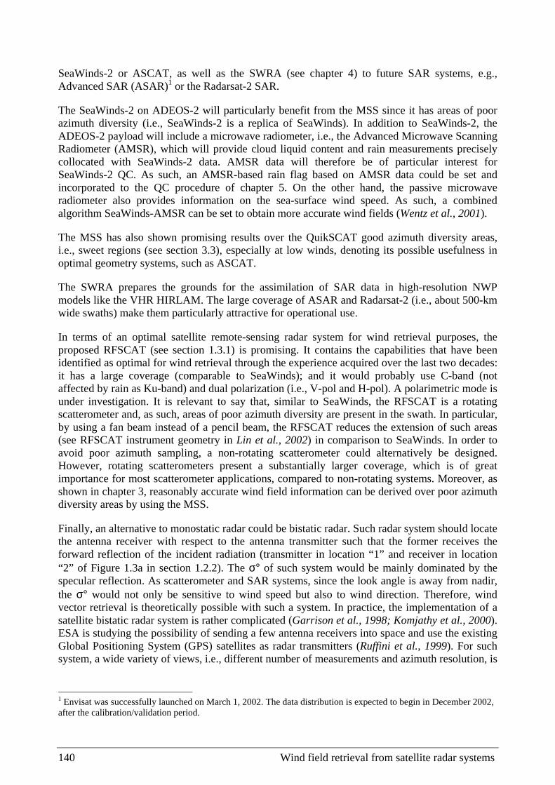
140 Wind field retrieval from satellite radar systems
SeaWinds-2 or ASCAT, as well as the SWRA (see chapter 4) to future SAR systems, e.g., Advanced SAR (ASAR)1 or the Radarsat-2 SAR.
The SeaWinds-2 on ADEOS-2 will particularly benefit from the MSS since it has areas of poor azimuth diversity (i.e., SeaWinds-2 is a replica of SeaWinds). In addition to SeaWinds-2, the ADEOS-2 payload will include a microwave radiometer, i.e., the Advanced Microwave Scanning Radiometer (AMSR), which will provide cloud liquid content and rain measurements precisely collocated with SeaWinds-2 data. AMSR data will therefore be of particular interest for SeaWinds-2 QC. As such, an AMSR-based rain flag based on AMSR data could be set and incorporated to the QC procedure of chapter 5. On the other hand, the passive microwave radiometer also provides information on the sea-surface wind speed. As such, a combined algorithm SeaWinds-AMSR can be set to obtain more accurate wind fields (Wentz et al., 2001).
The MSS has also shown promising results over the QuikSCAT good azimuth diversity areas, i.e., sweet regions (see section 3.3), especially at low winds, denoting its possible usefulness in optimal geometry systems, such as ASCAT.
The SWRA prepares the grounds for the assimilation of SAR data in high-resolution NWP models like the VHR HIRLAM. The large coverage of ASAR and Radarsat-2 (i.e., about 500-km wide swaths) make them particularly attractive for operational use.
In terms of an optimal satellite remote-sensing radar system for wind retrieval purposes, the proposed RFSCAT (see section 1.3.1) is promising. It contains the capabilities that have been identified as optimal for wind retrieval through the experience acquired over the last two decades: it has a large coverage (comparable to SeaWinds); and it would probably use C-band (not affected by rain as Ku-band) and dual polarization (i.e., V-pol and H-pol). A polarimetric mode is under investigation. It is relevant to say that, similar to SeaWinds, the RFSCAT is a rotating scatterometer and, as such, areas of poor azimuth diversity are present in the swath. In particular, by using a fan beam instead of a pencil beam, the RFSCAT reduces the extension of such areas (see RFSCAT instrument geometry in Lin et al., 2002) in comparison to SeaWinds. In order to avoid poor azimuth sampling, a non-rotating scatterometer could alternatively be designed. However, rotating scatterometers present a substantially larger coverage, which is of great importance for most scatterometer applications, compared to non-rotating systems. Moreover, as shown in chapter 3, reasonably accurate wind field information can be derived over poor azimuth diversity areas by using the MSS.
Finally, an alternative to monostatic radar could be bistatic radar. Such radar system should locate the antenna receiver with respect to the antenna transmitter such that the former receives the forward reflection of the incident radiation (transmitter in location “1” and receiver in location “2” of Figure 1.3a in section 1.2.2). The σ° of such system would be mainly dominated by the specular reflection. As scatterometer and SAR systems, since the look angle is away from nadir, the σ° would not only be sensitive to wind speed but also to wind direction. Therefore, wind vector retrieval is theoretically possible with such a system. In practice, the implementation of a satellite bistatic radar system is rather complicated (Garrison et al., 1998; Komjathy et al., 2000). ESA is studying the possibility of sending a few antenna receivers into space and use the existing Global Positioning System (GPS) satellites as radar transmitters (Ruffini et al., 1999). For such system, a wide variety of views, i.e., different number of measurements and azimuth resolution, is
1 Envisat was successfully launched on March 1, 2002. The data distribution is expected to begin in December 2002, after the calibration/validation period.

Chapter 6. Discussion and outlook 141
expected. As such, the wind retrieval methodology implemented in this thesis could be further explored for bistatic radar use.

142 Wind field retrieval from satellite radar systems

Appendix A. QuikSCAT data products 143
Appendix A
QuikSCAT Data Products
There are two QuikSCAT data products: the Hierarchical Data Format (HDF) and the Binary Universal Format Representation (BUFR). The former usually takes a few weeks to be delivered and is used for broad scientific purposes; the latter is a near-real time (NRT) product and, as such, takes only a few hours to be delivered, contains somehow reduced information (compared to the former product), and is used for operational purposes (e.g., data assimilation). A full description of the HDF and BUFR data products can be found in JPL (2001) and Leidner et al. (2000), respectively.
The work described in this thesis is focused on the Level 2A and Level 2B HDF Science products and on the NRT BUFR product. The Level 2A contains the radar backscatter (σ°) related information and the level 2B the surface wind related information, while the BUFR product contains both the σº and the wind information.
The main difference between the HDF and the BUFR product is related to the spatial resolution of σ°. In each WVC, the σ° of a particular view (fore-inner, fore-outer, aft-inner, aft-outer) in the BUFR product is an average of all σ°s of that particular view in the HDF product, which fall in the same WVC.
The SeaWinds σ°s can be either “eggs” or slices. In a particular WVC, an “egg” σ° is the radar backscatter from the whole pulse or footprint whose centre falls in that WVC. The “egg” can be subdivided in individual range-resolution elements or slices; the slices of a particular “egg” whose centre fall in the same WVC are weight- averaged (the weighting factor is directly dependent on the noise of each slice “measurement”) to become a pulse-composite σ°. The antenna footprint or “egg” is an ellipse approximately 25-km in azimuth by 37-km in the look (or range) direction. The slices are 25-km in azimuth by a variable range resolution of approximately 2 to 10 km (the nominal width is 6 km).
The HDF data are given in “egg” resolution. Therefore, although the size of the WVC is 25 km, the actual resolution of the winds retrieved from the “egg” σºs is approximately 40 km. Composites enhance the wind resolution mainly in range direction down to 25 km, and have little effect on azimuth resolution. The BUFR σ°s are weighted average of pulse-composites or WVC-composites.

144 Wind field retrieval from satellite radar systems
Figure A.1 shows a schematic illustration of the σ° processing. For example, the σ° information for a single view (fore-inner, aft-inner, fore-outer or aft-outer) at the top-right WVC is: two σ°s, which correspond to the two right-most “eggs”, for HDF; and one σ°, which corresponds to the WVC-composite of the (four) darkest slices, for BUFR.
Figure A.1 The slices for three pulses or footprints (“eggs”) of a single view are shown along with four WVCs (squares). The slices are shaded differently depending on which WVC contains the slice centroid. Slices with centroids outside the four WVCs are not striped. All slices with the same shading from a single pulse contribute to the pulse-composites for that pulse and WVC. Similarly, all slices with the same shading contribute to the WVC-composite (Figure 6 from Leidner et al., 2000).

Appendix B. Expected maximum likelihood estimator 145
Appendix B
Expected Maximum Likelihood Estimator
B.1 <MLE> surface fit for the 25-km JPL-retrieved winds in HDF format
In order to fit a 2D function to the filtered mean MLE surface (see Figure 2.5b), we first fit a function for the MLE dependence on wind speed at a certain node. Then we assume that the shape of this function is nearly constant over all nodes of the inner swath and we compute the variation of its mean value over the node number domain.
Figure B.1a shows the fit of the filtered mean MLE versus wind speed for node number 25 with a Gaussian + 2nd order polynomial function. The dotted line represents the extrapolated values for wind speeds higher than 20 m/s. It is clearly discernible that the fit is very accurate for that particular node.
Figure B.1b shows the averaged MLE over all wind speeds and normalized with the speed dependent function (fit on Figure B.1a) versus the node number in the inner swath. The fit is a 2nd order polynomial function (node dependent function). The dotted line shows the extrapolation over the outer swath.
The fact that we have found a 2D function which fits reasonably well to the computed mean MLE makes our assumption of considering the shape of the speed dependent function constant over the node domain valid.
The 2D function that fits the filtered mean MLE surface is simply the product of the speed and the node dependent functions. The expression is the following:
)(')( nfvfMLE fit ⋅=>< (B.1)
2543
)(2
1
0
2
2
1
)( vAvAAeAvf A
Av
⋅+⋅++⋅=−
⋅− (B.2)
2210)(' nBnBBnf ⋅+⋅+= ; ]76,1[∈∀ n (B.3)

146 Wind field retrieval from satellite radar systems
where f is the wind speed dependent function, f’ is the node dependent function, v is the wind speed and n the node number.
The coefficient values are the following:
A0 = 0.78519; A1 = 1.47396; A2 = 2.91577
A3 = 0.31881; A4 = -4.2426E-3; A5 = 6.9633E-5
B0 = 1.37840; B1 = -0.02713; B2 = 3.4853E-4
B.2 <MLE> calculation for the 25-km JPL-retrieved winds in BUFR format
Following the methodology described in section 2.3.1, we compute the <MLE> for the 25-km JPL-retrieved winds in BUFR format. In this section, we summarize the mentioned <MLE> computation, emphasizing the differences with the <MLE> in HDF format (see section 2.3.1 and Appendix B.1).
The <MLE> is also computed from 60 orbits of real data (BUFR in this case). From the mean MLE surface versus wind speed and node number, the noise is filtered using the same iterative process as for HDF. However, the MLEs rejected are three (or more) times higher than the mean MLE instead of two times as for HDF. This is done to keep consistency in the filtering procedure
a) b)
Figure B.1 Filtered mean JPL-selected MLE versus JPL-selected wind speed (plot a) for node number 25 (stars), where the solid line shows the function fit and the dotted line the extrapolation for wind speeds higher than 20 m/s; and averaged JPL-selected MLE over all JPL-selected wind speeds, normalized with the speed dependent function (fit on plot a),, versus the node number (plot b) in the inner swath (stars), where the solid line represents the function fit and the dotted line the extrapolation for the outer swath.

Appendix B. Expected maximum likelihood estimator 147
in terms of rejecting a small amount of data and conserving the shape of the original function (see discussion in section 2.3.1).
Figure B.2a shows the filtered mean JPL-selected MLE versus JPL-selected wind speed and node number for BUFR. Comparing this surface with the one for HDF (Figure 2.5b), both are very similar although the BUFR surface looks more irregular for speeds higher than 7 m/s. These irregularities make the two-dimensional function fit (see below) to the BUFR surface less accurate. As said in section 2.3.1, the function fit is required for extrapolation purposes. Figure B.2b shows the function fit (or <MLE> surface). It is clearly discernible that the irregularities seen in Figure B.2a are filtered out in the fit, but the main shape of both surfaces remains the same and therefore the accuracy of the resulting Rn is not expected to decrease significantly.
Both surfaces in Figure B.2 are for speeds lower than 20 m/s and for the inner nodes. The two-dimensional function fit is used in the same way as in HDF to extrapolate the expected MLE surface for winds higher than 20 m/s and the outer nodes.
<MLE> surface fit
Looking at the filtered mean MLE surface (see Figure B.2a), it is clearly discernible that assuming a constant shape of the MLE dependence on wind speed over all nodes of the inner swath (as in Appendix B.1) is not valid anymore.
In this case, we fit a Gaussian + 2nd order polynomial function to the filtered mean MLE for each node of the inner swath separately. Then, we fit a 2nd order polynomial function to the evolution of each coefficient of the previous function with respect to the node number. Therefore, the 2D function that fits the filtered mean MLE surface is the following:
2543
)(2
1
0
2
2
1
vAvAAeAMLE A
Av
fit ⋅+⋅++⋅=><−
⋅− (B.4)
2210 nAnAAA iiii ⋅+⋅+= ; ]76,1[],5,0[ ∈∀∈∀ ni (B.5)
where <MLE> is the expected MLE (see Figure B.2b), v is the wind speed and n the node number.
The coefficient values are the following:
A00 = 0.55000; A01 = 0.00000; A02 = 0.00000
A10 = 1.50000; A11 = 0.00000; A12 = 0.00000
A20 = 2.75000; A21 = 0.00000; A22 = 0.00000
A30 = 0.21210; A31 = -2.49E-3; A32 = 3.02E-5
A40 = -7.41E-3; A41 = 3.13E-4; A42 = -4.08E-6
A50 = 1.18E-4; A51 = -4.76E-6; A52 = 6.24E-8

148 Wind field retrieval from satellite radar systems
a)
b)
Figure B.2 “Filtered” mean JPL-selected MLE (plot a) and Expected MLE (plot b) versus JPL-selected wind speed and node number for the inner swath nodes. The speed binning is 1 m/s and the node binning is 1.

Appendix B. Expected maximum likelihood estimator 149
B.3 <MLE> calculation for the 25-km KNMI-retrieved winds in BUFR format
As in Appendix B.2, we follow the methodology described in section 2.3.1 to compute the <MLE> for our KNMI-inverted winds. In contrast with the <MLE> used in chapter 5, we use the 1st rank MLE and wind speed information to compute the <MLE> since we do not have information on the “selected” solution (no KNMI 25-km AR at this stage). However, as discussed in section 5.1.3, the Rn based on the 1st rank solution is comparable to the Rn based on the selected solution in terms of QC skill. Therefore, it is irrelevant whether we use an <MLE> based on the selected or the 1st rank solution for computing the solution probability.
Figure B.3a shows the “filtered” mean KNMI 1st rank MLE as a function of node number and KNMI 1st rank wind speed for QuikSCAT BUFR data, at the inner swath. In contrast with Figures 2.5b and B.2a, there is no straightforward way to fit a two-dimensional function (see Appendices B.1 and B.2) to this surface. We could directly use this surface as <MLE> by creating a table. However, there is some remaining noise in the surface, especially at low and high winds that we would like to remove. It is also important to remove this noise if we want to consistently extrapolate the <MLE> for winds higher than 20 m/s. Therefore, we have fit a Gaussian + 2nd order polynomial function in the speed domain for every node of the inner swath. Since it is not practical to use 60 different functions (one for every inner swath node) and the mean MLE is rather constant for high winds, we have created a two-dimensional array (table) with speed bins of 1 m/s and node bins of 1, which ranges from nodes 1 to 76 and from speeds 0 m/s to 20 m/s. For any wind speed higher than 20 m/s, the <MLE> value used is the one at 20 m/s for that particular node number. There are not yet plans to use the Rn in the outer swath and therefore no attempt to extrapolate the <MLE> in the outer swath has been made. However, as a first guess, we have copied the <MLE> values at the edges of the inner swath to the outer swath nodes. Figure B.3b shows the <MLE> surface derived from the <MLE> array, over the inner swath. The surface compares well with the mean MLE surface (Figure B.3a).
B.4 <MLE> calculation for the 100-km KNMI-retrieved winds in BUFR format
The <MLE> for 100-km is computed in a similar way to the Rn for 25-km (see Appendix B.3). Figure B.4a shows the “filtered” mean KNMI 1st rank MLE surface as a function of the KNMI 1st rank wind speed and the node number for 100-km resolution inverted winds. [Note that the 100-km node numbers 4 to 16 correspond to most of the QuikSCAT inner swath]. As in Figure B.3a, there is no straightforward way to fit a two-dimensional function to the surface. Therefore, we compute a table in a similar way as for the 25-km product <MLE> (see Appendix B.3). However, as we can see in Figure B.4a, no significant noise is present in the surface. Therefore, we do not even perform a function fit in the speed domain, as it is done for the 25-km surface (see Appendix B.3), but rather leave the surface as it is. We only perform an average over the last three speed bins (wind speeds from 17 m/s to 20 m/s) to filter the remaining noise at high winds and therefore be able to consistently extrapolate for winds higher than 20 m/s. Therefore, the <MLE> table (shown in Figure B.4b) is almost a copy of the mean MLE surface (Figure B.4a).

150 Wind field retrieval from satellite radar systems
a)
b)
Figure B.3 “Filtered” mean KNMI 1st rank MLE (plot a) and Expected MLE (plot b) as a function of node number and KNMI 1st rank wind speed for BUFR data (inner swath), at 25-km resolution. The speed binning is 1 m/s and the node binning is 1.
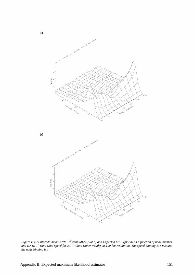
Appendix B. Expected maximum likelihood estimator 151
a)
b)
Figure B.4 “Filtered” mean KNMI 1st rank MLE (plot a) and Expected MLE (plot b) as a function of node number and KNMI 1st rank wind speed for BUFR data (inner swath), at 100-km resolution. The speed binning is 1 m/s and the node binning is 1.

152 Wind field retrieval from satellite radar systems

Appendix C. Inversion tuning 153
Appendix C
Inversion Tuning
Although the QuikSCAT inversion problem discussed in section 2.2 is inherent of the inversion process and therefore not solvable at this stage, a further examination of such process is desirable in order to optimize it for QuikSCAT.
NSCAT-2 versus QSCAT-1
Since May 2000, the JPL QuikSCAT winds are retrieved using the QSCAT-1 GMF. This is the first empirically derived GMF from QuikSCAT measurements (Freilich et al., 2002), as the one used before the mentioned date, NSCAT-2, was derived from NSCAT data (Wentz and Smith, 1999). Since we have had access to both the NSCAT-2 and the QSCAT-1 tables (remember that the GMFs are tabulated for computational efficiency purposes), it seems reasonable to compare them, using the KNMI inversion software, in order to choose the most appropriate for QuikSCAT wind retrieval. A set of 12 hours of QuikSCAT data is collocated with ECMWF winds and used in here for reference.
Figure C.1 shows the wind direction distributions with respect to the satellite flight direction of ECMWF winds (solid lines) and QuikSCAT retrieved solutions closest to ECMWF (dotted lines). The QuikSCAT winds from the top plots are retrieved using NSCAT-2 GMF; the ones from the bottom plots are retrieved using QSCAT-1 GMF. It is discernible from the left plots (i.e., wind direction distributions for WVC number 20) that the QSCAT-1 wind direction distribution fits better the ECMWF distribution than the NSCAT-2 distribution, where some unrealistic accumulations are discernible (see peaks around 60°, 120° and 230° in Figure C.1a). Looking at the direction distributions over the entire inner swath (right plots), we still see a better fit of QSCAT-1distributions, denoting that the QSCAT-1 wind directions are somewhat more realistic than NSCAT-2 directions.
This result is in line with the RMS difference values between QuikSCAT and ECMWF wind directions. As expected, the RMS difference in wind direction is lower for QSCAT-1 than for NSCAT-2 in both the sweet and the nadir swaths (see table C.1).
154 Wind field retrieval from satellite radar systems
a) b)
c) d)
Figure C.1 Wind direction (with respect to the satellite flight direction) histograms of ECMWF winds (solid lines) and QuikSCAT-retrieved solutions closest to ECMWF (dotted lines) for WVC number 20 (left plots) and for the inner swath (right plots). The QuikSCAT winds have been retrieved using NSCAT-2 GMF (top plots) and QSCAT-1 GMF (bottom plots). Non-smoothing and 3D interpolation have been used in the inversion.
Tables C.2 to C.5 show the percentage of “selected” solutions (closest to ECMWF) stratified by number of solutions and rank. The number of solutions corresponds to the number of minima in the MLE cost function and the solution ranking goes from the deepest to the shallowest cost function minimum in ascending order. The first row corresponds to the number of data stratified by number of solutions. Tables C.2 and C.3 correspond to the NSCAT-2 GMF selected solution distributions of the sweet and nadir swaths, respectively. Tables C.4 and C.5 correspond to QSCAT-1 GMF selected solution distributions of the sweet and nadir swaths, respectively.
As discussed in section 2.2.2, the 1st rank skill shows the ambiguity or uncertainty of the inversion. In these tables, the 1st rank skill is shown by the percentage of selections of rank 1 solution. As we see in the tables, in general the 1st rank skill is higher for NSCAT-2 than for QSCAT-1 in the sweet swath and comparable in the nadir swath (see overall results in the last

Appendix C. Inversion tuning 155
column of the tables). Moreover, the number of solutions given by the NSCAT-2 GMF is significantly smaller than the number given by QSCAT-1 in both the sweet and the nadir swaths (see the relative accumulation of data for 3 and 4 solutions of QSCAT-1 tables compared to NSCAT-2 tables). This shows that NSCAT-2 GMF produces a much less ambiguous wind product than QSCAT-1.
Figure C.2 shows the two-dimensional histograms of the QuikSCAT retrieved wind solution closest to ECMWF versus the ECMWF winds for zonal (left plots) and meridional (right plots) components. The QuikSCAT winds from the top plots are retrieved using the NSCAT-2 GMF; the ones from the bottom plots are retrieved using the QSCAT-1 GMF. As discussed in section 2.2.2, the quality of the closest gives an idea of the accuracy of the retrieved winds. No significant difference is discernible when comparing NSCAT-2 (top) and QSCAT-1 (bottom) plots. However, if we look at the legend we see slightly lower SD values for NSCAT-2 compared to QSCAT-1. [Note: these histograms correspond to the sweet parts of the swath; similar conclusions can be derived from the nadir swath histograms (not shown)]. Although the RMS difference in direction is lower for QSCAT-1 than for NSCAT-2 winds, the RMS difference in speed is lower for NSCAT-2 than for QSCAT-1 (see table C.1), leading to an overall comparable accuracy, slightly higher for NSCAT-2 winds.
Stoffelen et al. (2000) computed a more realistic RMS difference in wind direction, called the normalized RMS (NRMS). Using the actual RMS definition, the more ambiguous solutions are provided by the inversion, the smaller the RMS will be, because the chance that one of the solutions will be close to the wind reference will increase. In the limit of an infinite amount of observations, the RMS will even be zero, while the information content of the set of solutions in reality decreases with an increasing number of solutions, because there is no a priori way to say which of the solutions is the correct one. In order to solve this problem, they normalize the RMS with an expected value, which is dependent on the angle separation of the neighboring solutions of the closest solution to reference (ECMWF in this case). For more details, see Stoffelen et al. (2000). If we compute the NRMS, we get lower values for the less ambiguous NSCAT-2 product than for QSCAT-1 (see table C.1).
Both the RMS and the NRMS parameters are not the true and only way to look at the accuracy of the retrieved winds. Moreover, the ECMWF is just a reference. Therefore, it is difficult to say precisely from the results, which of the two GMFs produces more accurate winds. However, it is clear that both GMFs produce winds of comparable accuracy.
Table C.1 Statistics for NSCAT-2 and QSCAT-11.
RMS in Speed (m/s) NSCAT-2/QSCAT-1
RMS in Direction(°) NSCAT-2/QSCAT-1
NRMS NSCAT-2/QSCAT-1
Sweet swath 1.57 / 1.66 21.39 / 19.36 0.4953 / 0.5113
Nadir swath 1.67 / 1.73 29.14 / 27.56 0.5359 / 0.5619
1 Non-smoothing and 3D interpolation have been used in the inversion.

156 Wind field retrieval from satellite radar systems
Table C.2 Solution distribution for NSCAT-2 GMF (sweet swath)1. 1 Solution 2 Solutions 3 Solutions 4 Solutions All Solutions
Number of Data 378 62856 44029 61172 168435
Rank 1 100 90 81 79 84
Rank 2 - 10 14 16 13
Rank 3 - - 5 3 2
Rank 4 - - - 2 1
Table C.3 Solution distribution for NSCAT-2 GMF (nadir swath)1. 1 Solution 2 Solutions 3 Solutions 4 Solutions All Solutions
Number of Data 6877 48382 30943 8303 94505
Rank 1 100 81 79 64 80
Rank 2 - 19 16 19 17
Rank 3 - - 5 9 2
Rank 4 - - - 8 1
Table C.4 Solution distribution for QSCAT-1 GMF (sweet swath)1. 1 Solution 2 Solutions 3 Solutions 4 Solutions All Solutions
Number of Data 29 45139 48795 74473 168436
Rank 1 100 94 81 74 81
Rank 2 - 6 14 18 14
Rank 3 - - 5 5 4
Rank 4 - - - 3 1
Table C.5 Solution distribution for QSCAT-1 GMF (nadir swath)1. 1 Solution 2 Solutions 3 Solutions 4 Solutions All Solutions
Number of Data 4000 45806 36279 8413 94498
Rank 1 100 82 78 70 80
Rank 2 - 18 16 20 17
Rank 3 - - 6 6 3
Rank 4 - - - 4 0
1 Non-smoothing and 3D interpolation have been used in the inversion.

Appendix C. Inversion tuning 157
In summary, the NSCAT-2 provides a less ambiguous product than QSCAT-1 without decreasing the quality of the wind retrieval. In other words, in comparison with QSCAT-1, NSCAT-2 is capable of removing a significant amount of unrealistic ambiguous wind solutions. Moreover, as discussed in Appendix D, the NSCAT-2 GMF better fits the backscatter measurements than the QSCAT-1 GMF. Consequently, the NSCAT-2 GMF will be used for deriving QuikSCAT winds.
a) b) sweet swath
−20 −10 0 10 20U comp. (m/s) − ECMWF
−20
−10
0
10
20
U c
omp.
(m
/s)
− K
NM
I
N= 168500mx= −1.11 my= −1.03m(y−x)= 0.08 s(y−x)= 1.83cor_xy= 0.96
sweet swath
−20 −10 0 10 20V comp. (m/s) − ECMWF
−20
−10
0
10
20
V c
omp.
(m
/s)
− K
NM
I
N= 168500mx= −0.21 my= −0.20m(y−x)= 0.02 s(y−x)= 1.89cor_xy= 0.94
c) d)
sweet swath
−20 −10 0 10 20U comp. (m/s) − ECMWF
−20
−10
0
10
20
U c
omp.
(m
/s)
− K
NM
I
N= 168500mx= −1.11 my= −1.10m(y−x)= 0.01 s(y−x)= 1.84cor_xy= 0.96
sweet swath
−20 −10 0 10 20V comp. (m/s) − ECMWF
−20
−10
0
10
20
V c
omp.
(m
/s)
− K
NM
I
N= 168500mx= −0.21 my= −0.22m(y−x)= −0.01 s(y−x)= 1.95cor_xy= 0.94
Figure C.2 Two-dimensional histogram of the closest KNMI-retrieved wind solution to ECMWF wind versus ECMWF wind for QuikSCAT winds derived with the NSCAT-2 (top plots) and the QSCAT-1 (bottom plots) GMFs. The left plots correspond to the zonal wind component and the right plots to the meridional wind component (bins of 0.4 m/s for both components). The legend and the contour lines are the same as in Figure 2.2. Non-smoothing and 3D interpolation have been used in the inversion.

158 Wind field retrieval from satellite radar systems
Smoothing versus interpolation
The MLE cost function is often noisy (imagine very small peaks and troughs in Figure 2.1). This leads to the detection of excessive minima close to each other in the inversion process, especially in the nadir swath where the minima tend to be broad. A common way to solve the problem is to apply a smoothing technique over the cost function. The idea is to define a smoothing window whose size is determined by the number of cost function points below a certain threshold. This threshold can be defined for example as a factor of the minimum MLE value, the minimum Rn value, or the difference between the maximum and the minimum MLE values in the cost function. Here we test a couple of smoothing techniques, whose main difference is the resulting window sizes, and compare them to a non-smoothing inversion (smoothing window size is zero). Figure C.3 shows the smoothing window size distribution over the mentioned 12-hour period of QuikSCAT data and the entire inner swath for two different techniques. Since we use the same wind direction step size as the one defined in the table (2.5°) to compute the MLE cost function, the latter has a total of 144 points. The number of points used in the smoothing is = 2 x window size + 1. The difference between technique I (Figure C.3a) and technique II (Figure C.3b) lays in the window size distribution, whose mean value is around 1-2 in the former and 4-5 in the latter.
Figure C.4 shows the same wind direction distributions as Figure C.1a but for no smoothing (plot a), smoothing technique I (plot b) and smoothing technique II (plot c). It is clearly discernible from the plots that there is an increase of unrealistic retrieved wind directions as we increase the window size (see evolution of peaks centered around 60°, 120° and 230° from Figures C.4a to C.4c). This shows how sensitive can be the smoothing to the quality of the retrieval. As we increase the smoothing window, the MLE cost function changes shape and the minima are therefore shifted. Due to the non-linearity of the cost function, some wind directions are favoured in the smoothing process, leading to an increase of unrealistic accumulations at certain directions as shown in Figure C.4b and C.4c.
a) b)
Figure C.3 Normalized histograms of the smoothing window size for the smoothing techniques I (plot a) and II (plot b) over the entire inner swath.

Appendix C. Inversion tuning 159
An alternative to the smoothing is the interpolation of the GMF LUT. As mentioned in section 2.2, to compute the MLE cost function, we search for a minimum in the speed domain and then we repeat this operation for the entire wind direction spectrum. This is usually performed at the LUT resolution level for speed (0.2 m/s) and direction (2.5°), and only the incidence angles are interpolated (the step size is 1° in the LUT). However, the GMF is also sensitive to speed and direction changes and this may lead to inaccuracies in the selection of the minimum, which in turn can produce noise in the MLE cost function. Therefore, we perform a three-dimensional linear interpolation in the incidence angle, speed and direction domains. Since the GMF is especially sensitive to speed changes, we refine the minimum search in speed to a resolution of 0.02 m/s. [Note that tests at a higher resolution search in the speed domain, up to 0.001 m/s, have been performed with similar results].
Figures C.4a and C.1a show the retrieved wind direction distributions (compared to ECMWF) for interpolating in 1D (only incidence angle) and in 3D (incidence angle, speed and direction), respectively. The QuikSCAT wind direction distributions look almost identical. In contrast with
a)
b) c)
Figure C.4 Same as Figure C.1a but for no smoothing (plot a), smoothing technique I (plot b) and smoothing technique II (plot c). The 1D interpolation scheme has been used in the inversion.

160 Wind field retrieval from satellite radar systems
smoothing, the 3D interpolation is not adding any unrealistic accumulation of retrieved directions. This is an expected result, since the interpolation is looking for a more precise minimum but not changing the shape of the MLE cost function.
Tables C.6 and C.7 are similar to the tables C.2 and C.3 respectively. In the former, 1D interpolation has been used, while 3D interpolation is used in the latter. The 3D interpolation scheme has much less number of solutions (see the decrease in the number of data with 4 solutions in the 3D tables compared to the 1D tables) and a higher 1st rank skill (see higher percentages of rank-1 solutions for the 3D tables compared to the 1D tables), resulting in a less ambiguous product compared to the 1D product. In the nadir region, since the minima tend to be broad, the noise in the cost function is expected to produce more ambiguity than in the sweet swath where minima are steeper. Notice the significant reduction of ambiguity in the nadir of the 3D scheme with respect to the 1D scheme, denoting a clear reduction of the cost function noise.
Table C.8 is similar to the left column (NSCAT-2 results) of table C.1. Again, the former corresponds to the results of the 1D scheme, and the latter to the results of the 3D scheme. When comparing the two tables, we notice no significant differences, and therefore no significant difference in the quality of both interpolation schemes. The speed RMS values are almost
Table C.6 Solution distribution for NSCAT-2 GMF (sweet swath)1.
1 Solution 2 Solutions 3 Solutions 4 Solutions All Solutions
Number of Data 132 50786 40677 76835 168430
Rank 1 100 92 77 73 80
Rank 2 - 8 18 18 15
Rank 3 - - 5 6 4
Rank 4 - - - 3 1
Table C.7 Solution distribution for NSCAT-2 GMF (nadir swath)1.
1 Solution 2 Solutions 3 Solutions 4 Solutions All Solutions
Number of Data 571 18900 20599 54437 94507
Rank 1 100 81 71 42 56
Rank 2 - 19 24 23 22
Rank 3 - - 5 18 12
Rank 4 - - - 17 10
1 Non-smoothing and 1D interpolation have been used in the inversion.

Appendix C. Inversion tuning 161
identical and the direction RMS is somewhat higher in the 3D scheme compared to the 1D scheme. In contrast, the NRMS of the 3D scheme is lower compared to that of the 1D scheme, especially in the nadir region, as expected from the lower ambiguity of the 3D scheme already mentioned.
If we go back to the discussion on the smoothing, the smoothing technique I produces similar ambiguity, speed RMS and NRMS values (not shown) than the 3D scheme. However, the RMS in direction for the smoothing technique I is 10% higher than for the 3D scheme due to the unrealistic direction accumulations already discussed. The smoothing technique II produces the least ambiguous product of all. This is reflected in only a small decrease of the NRMS (drop of 2% in the sweet swath and 5% in the nadir region) in comparison with the 3D scheme. However, the direction RMS difference of the smoothing technique II is about 20% higher than that of the 3D scheme.
Therefore, we can say that the 3D scheme is the only examined scheme, which considerably reduces the ambiguity of the retrieved winds without affecting their quality in comparison to the flat scheme (1D interpolation). The smoothing techniques are meant to remove undesired wind solutions. However, this is not evident for QuikSCAT at low winds, where the solution pattern (we have examined many cases) is very noisy and does not show clearly undesirable solutions, which may be removed by smoothing, with the consequent decrease in quality. [Note that the smoothing techniques have also been tested in combination with the 3D interpolation resulting in similar problems than when combined with the 1D interpolation]. Therefore, for QuikSCAT, it is better to keep all the information (no smoothing) and use the 3D scheme.
Table C.8 Statistics for NSCAT-21.
RMS in Speed (m/s) NSCAT-2
RMS in Direction(°) NSCAT-2
NRMS NSCAT-2
Sweet swath 1.57 20.89 0.5095
Nadir swath 1.65 25.57 0.8422
1 Non-smoothing and 1D interpolation have been used in the inversion.

162 Wind field retrieval from satellite radar systems

Appendix D. Quality control with QSCAT-1 163
Appendix D
Quality Control with QSCAT-1
The QC procedure of section 5.1 is based on the MLE information derived with the NSCAT-2 GMF. If we invert winds using a different GMF, i.e., QSCAT-1, we will get different MLE values. Although these differences are not expected to be significant, it may well be that Quality Control is affected and therefore it needs to be revised.
Assuming no major changes, we first compute the Rn (see equation 2.10) using the new QSCAT-1 GMF MLE data and the existing <MLE> surface (i.e., computed from NSCAT-2 GMF data in Appendix B.1). The test is performed for two weeks of QuikSCAT HDF data.
Rn Characterization
As in section 5.1.2, we collocate QuikSCAT data with ECMWF winds and SSM/I rain data and look at the same kind of plots as in Figures 5.1 to 5.4 in order to characterize the Rn. The plots show very similar features as in section 5.1.2. The only difference is a slight increase in the Rn values.
Figure D.1 shows the contour plot of a two-dimensional histogram of RMS-ECMWF against Rn. As in Figure 5.1 (same plot but for the NSCAT-2 GMF), the RMS-ECMWF increases (quality of data decreases) as Rn increases and the RMS-ECMWF is increasing more rapidly with Rn at higher wind speeds (see plots b, c and d). However, when comparing both Figures, it is discernible that the distributions (see contour lines) in Figure D.1 are slightly shifted towards higher Rn values compared to Figure 5.1. The shift is more significant at mid and high wind speeds (see plots c and d of both Figures).
As we have used the same <MLE> surface to compute the Rn, the above-mentioned shift means that in general the MLE values coming out from the inversion are slightly higher using the QSCAT-1 GMF than using the NSCAT-2 GMF. This is an indication that the NSCAT-2 GMF better fits the backscatter measurements than the QSCAT-1 GMF (see chapter 2). Therefore, if we keep the same Rn threshold as in section 5.1, we would expect to have more rejections in this case.

164 Wind field retrieval from satellite radar systems
Threshold Validation
Similar to section 5.1.3, we test the same Rn threshold as defined in section 5.1.2 (see equation 5.1) against ECMWF and SSM/I collocations. The results for the sweet parts of the swath are shown in tables D.1, D.2 and D.3, and the results for the nadir part are shown in tables D.4, D.5 and D.6. Tables D.1-D.6 are in the same format as tables 5.1-5.6 (see section 5.1.3), respectively.
a) b)
c) d)
Figure D.1 Same as Figure 5.1 but for the QSCAT-1 GMF.
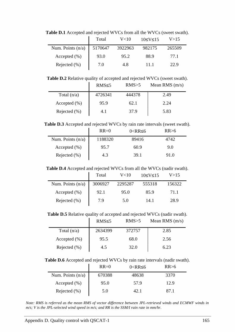
Appendix D. Quality control with QSCAT-1 165
Table D.1 Accepted and rejected WVCs from all the WVCs (sweet swath). Total V<10 10≤V≤15 V>15
Num. Points (n/a) 5170647 3922963 982175 265509
Accepted (%) 93.0 95.2 88.9 77.1
Rejected (%) 7.0 4.8 11.1 22.9
Table D.2 Relative quality of accepted and rejected WVCs (sweet swath).
RMS≤5 RMS>5 Mean RMS (m/s)
Total (n/a) 4726341 444378 2.49
Accepted (%) 95.9 62.1 2.24
Rejected (%) 4.1 37.9 5.83
Table D.3 Accepted and rejected WVCs by rain rate intervals (sweet swath).
RR=0 0<RR≤6 RR>6
Num. Points (n/a) 1188320 89416 4742
Accepted (%) 95.7 60.9 9.0
Rejected (%) 4.3 39.1 91.0
Table D.4 Accepted and rejected WVCs from all the WVCs (nadir swath).
Total V<10 10≤V≤15 V>15
Num. Points (n/a) 3006927 2295287 555318 156322
Accepted (%) 92.1 95.0 85.9 71.1
Rejected (%) 7.9 5.0 14.1 28.9
Table D.5 Relative quality of accepted and rejected WVCs (nadir swath).
RMS≤5 RMS>5 Mean RMS (m/s)
Total (n/a) 2634399 372757 2.85
Accepted (%) 95.5 68.0 2.56
Rejected (%) 4.5 32.0 6.23
Table D.6 Accepted and rejected WVCs by rain rate intervals (nadir swath).
RR=0 0<RR≤6 RR>6
Num. Points (n/a) 670388 48638 3370
Accepted (%) 95.0 57.9 12.9
Rejected (%) 5.0 42.1 87.1
Note: RMS is referred as the mean RMS of vector difference between JPL-retrieved winds and ECMWF winds in m/s; V is the JPL-selected wind speed in m/s; and RR is the SSM/I rain rate in mm/hr.

166 Wind field retrieval from satellite radar systems
Comparing table D.1 to table 5.1, we appreciate a larger percentage of rejections in the former at all speeds, and more in particular at mid and high winds. From tables D.2 and 5.2, we see a considerable amount of this excess of rejections concentrated below the RMS value of 5 m/s, which in turn makes the RMS-ECMWF slightly smaller. The RMS-ECMWF difference between accepted and rejected solutions is slightly smaller in table D.2 (3.6 m/s) compared to table 5.2 (4 m/s). This indicates a somewhat better performance of the HDF QC using the NSCAT-2 GMF. However, this excess in rejections is positively contributing to rain detection. From tables D.3 and 5.3, the amount of “rainy” WVCs rejected is higher in the former, especially at rain rates below 6 mm/hr where there is 9.7% more of rejections.
Comparing the HDF QC using the QSCAT-1 GMF in the nadir (tables D.4- D.6) with the HDF QC using the NSCAT-2 GMF (tables 5.4-5.6), we can draw the same conclusions than for the sweet parts of the swath. In terms of quantitative results, the only significant differences with respect to the sweet parts are the following: the excess of rejections is 1.6 % in total (see tables 5.4 and D.4) while in the sweet parts is 1.4% (see tables 5.1 and D.1); and the excess of rejections for rain rates below 6 mm/hr is 6.6% (see tables 5.6 and D.6) compared to the 9.7% in the sweet parts (see tables 5.3 and D.3).
In general, the results show that with the QSCAT-1 GMF the QC rejects more data than with the NSCAT-2 GMF. However, this gives a positive impact on rain detection, especially for rain rates below 6 mm/hr. Therefore, we believe that using the same QC procedure (i.e., same <MLE> surface and Rn threshold) as in section 5.1 for the new GMF (QSCAT-1) is appropriate and there is no need to tune the QC procedure to the new data.

Resumen (Summary in Spanish) 167
Resumen (Summary in Spanish)
1 Introducción
La mayoría de los sistemas radar embarcados en satélites y utilizados en teledetección son capaces de proporcionar información sobre el campo de viento en la superficie del mar. Esta tesis revisa los métodos de obtención o extracción del viento a partir de las mediciones de dichos sistemas y propone nuevos métodos para mejorar la calidad de las extracciones en los casos donde la metodología actual es insuficiente.
1.1 Importancia de las observaciones del viento en superficie
El flujo atmosférico está determinado por los campos de viento y de masa (o densidad) de aire. Las mediciones de viento son particularmente importantes para definir la circulación atmosférica a cualquier escala en los trópicos y fuera de ellos a escalas sub-sinópticas. En este sentido, el sistema de observación global (GOS), que incluye observaciones de distintas variables meteorológicas (por ejemplo presión, temperatura o viento) provenientes de sistemas de observación en superficie (estaciones meteorológicas terrestres, boyas, plataformas petrolíferas, barcos, etc.), aéreos (radiosondas o aviones) y espaciales (satélites), tiene en éstos últimos una de las mayores fuentes de información del viento. En concreto, la mayor fuente de información del viento sobre la superficie marina, que representa alrededor de un 70% de la superficie terrestre, proviene de las observaciones de los radares embarcados en satélites.
Los campos de viento (observaciones) obtenidos a partir de mediciones de radar tienen numerosas aplicaciones tanto en meteorología como en oceanografía. Así, la predicción del tiempo a corto y medio plazo, la modelización de la circulación oceánica o de las olas, la modelización de la interacción entre la superficie marina y el aire, la climatología o estudios más locales como las brisas o los flujos catabáticos son ejemplos de aplicaciones de dichas observaciones. Sin duda, una de las aplicaciones más importantes de este tipo de observaciones es la integración de datos en modelos numéricos de predicción del tiempo. Como se sabe, muchas de las borrascas de latitudes medias o fenómenos meteorológicos más extremos como las tormentas tropicales o los huracanes se originan en el océano. Estos suelen tener un gran impacto tanto social como económico, en ocasiones agravado por las predicciones imprecisas o erróneas.

168 Wind field retrieval from satellite radar systems
La integración de datos de viento en superficie puede ayudar a mejorar la predicción de la intensidad y posición de dichos fenómenos.
1.2 Relación entre la señal de radar y el viento
El radar (transmisor) emite radiación electromagnética en la región de las microondas hacia la Tierra. Esta radiación, típicamente de una longitud de onda de unos pocos centímetros, es dispersada y reflejada por la superficie rugosa marina de forma que una fracción de la potencia emitida será detectada por el radar (receptor). En esta región de las microondas, la absorción de radiación por parte de la atmósfera es pequeña. En la ecuación radar, que determina la relación entre la potencia emitida y la recibida, el coeficiente que hace referencia a la rugosidad de la superficie se llama sección eficaz del radar (σ°). En el caso de radares monostáticos (emisor y receptor en el mismo lugar), que son los únicos radares embarcados en satélites utilizados en observación de la Tierra hasta la fecha, este coeficiente se suele denominar coeficiente de retrodispersión.
La resolución del radar se obtiene por medición de tres magnitudes: el ángulo, la distancia y la velocidad. La primera hace referencia a la anchura (angular) del haz electromagnético y, por tanto depende del tipo de antena; la segunda se refiere al cálculo del retraso de la señal; y la tercera, al cálculo de la velocidad relativa entre el radar y la superficie “iluminada”. Los radares de apertura real (RAR) utilizan la discriminación en ángulo y en distancia, mientras que los radares de apertura sintética (SAR) utilizan la discriminación en distancia y en velocidad. Así, la resolución típica de los dispersómetros (un tipo de RAR) es de 25-50 km mientras que la de los sistemas SAR es típicamente de unos cuantos metros.
El coeficiente de retrodispersión, básicamente ligado a la rugosidad del mar, está caracterizado fundamentalmente por dos fenómenos: la dispersión de Bragg (mecanismo de resonancia entre la onda incidente y las olas de longitud de onda similar, es decir, las olas de capilaridad-gravedad) y la reflexión especular (efecto “espejo” que dependerá de la orientación de las olas respecto al radar). El viento, a su vez, interacciona con la superficie del mar. Es decir, cuando el viento empieza a soplar sobre el mar, las olas de capilaridad-gravedad se forman instantáneamente. Parte de la energía del viento es absorbida por el mar y es transferida espacial y temporalmente de las olas más pequeñas (olas de capilaridad-gravedad) a las olas de gravedad (decimétricas) y sucesivamente a las más largas (métricas, etc.). Cuanto mayor sea el módulo del viento mayor será el tamaño de olas que se formarán. La rugosidad del mar consecuentemente dependerá sobretodo del viento. La relación entre la señal del radar y el viento es pues indirecta y viene determinada por el efecto del viento sobre la rugosidad del mar que a su vez tiene un efecto sobre la señal electromagnética incidente. Esta relación, denominada función del modelo geofísico o GMF (Geophysical Model Function) es muy difícil de modelar teóricamente entre otros motivos por la compleja interacción entre las olas de diferente tamaño (que forman la rugosidad marina). Sin embargo, la modelización empírica es una buena alternativa para determinar dicha relación. La GMF empírica que relaciona el vector viento a 10 metros (sobre el mar) y el coeficiente de retrodispersión se formula generalmente de la siguiente manera:
[ ]Zo BBB )2cos()cos(1 210 φφσ ++= (1)
Resumen (Summary in Spanish) 169
donde φ es la dirección del viento (φ=0° cuando el viento sopla en la dirección del radar), y los coeficientes B0, B1 y B2 dependen del módulo del viento y del ángulo de incidencia, la polarización y la frecuencia del haz del radar. El valor del exponente z y el número de armónicos (la ecuación 1 puede contener armónicos adicionales) dependen del método de determinación empírica utilizado. Así pues, existen varias GMF empíricas para los distintos radares.
1.3 Tipos de radares en teledetección espacial
Existen varios tipos de radares embarcados en satélite y utilizados en observación de la Tierra. Sin embargo, para la obtención de la dirección del viento se necesita un radar cuyo haz no sea vertical sino inclinado (ángulo de incidencia entre los 16° y los 70°). Así pues, existen dos tipos de radar capaces de observar el campo de viento sobre el mar: los dispersómetros y el SAR.
En términos de la geometría de las antenas, los dispersómetros se pueden dividir en dos tipos: los de “mirada” lateral y los de rotación. Los primeros tienen las antenas fijas y por tanto la orientación relativa de los diferentes haces es invariable. Los segundos, tienen uno o varios haces en rotación, lo cual produce una orientación relativa de los haces que depende de la posición perpendicular a la traza del satélite. Actualmente sólo hay un radar de cada tipo en órbita: el SCAT, de “mirada” lateral, embarcado en el satélite europeo ERS-2, y el SeaWinds, de rotación, embarcado en el satélite americano QuikSCAT. Ambos tipos de dispersómetros tienen ya garantizada su continuidad con misiones futuras como ASCAT embarcado en METOP (2005) o SeaWinds-2 embarcado en ADEOS-2 (fin del 2002), respectivamente1.
En cuanto al SAR, actualmente hay varias misiones en órbita, como ERS-2, Envisat o Radarsat-1. En cuanto a futuras misiones SAR, Radarsat-2 está programado para ser lanzado en el 2004.
1.4 Obtención del viento
El proceso de obtención del vector viento a partir de las mediciones o coeficientes de retrodispersión del radar consiste en dos pasos: inversión y eliminación de la ambigüedad. El primer paso es calcular el vector viento a partir de las mediciones con la ayuda de la ecuación (1). Puesto que para ello se deben determinar el módulo y la dirección (dos incógnitas), se necesitarán al menos dos mediciones independientes para que el sistema esté determinado. Además, y debido a la alta no linealidad de la GMF y a los errores característicos de estas mediciones, la inversión suele dar hasta cuatro soluciones posibles del vector viento. Así pues, el segundo paso consiste en utilizar información adicional sobre el campo de viento (normalmente proveniente de modelos de predicción) así como criterios de balance meteorológico (por ej., geostrofía) y consistencia espacial para seleccionar una de las soluciones de la inversión como el vector viento observado.
1 Nota: SeaWinds se suele denominar QuikSCAT para diferenciarlo de SeaWinds-2, aunque ambos instrumentos son idénticos.

170 Wind field retrieval from satellite radar systems
La separación angular (o azimutal) entre los distintos haces del radar es muy importante a la hora de invertir el viento. Dos haces que observan un mismo lugar en la superficie con muy poca separación angular son en la práctica equivalentes a un solo haz. El grado de independencia de los haces dependerá entonces de la separación angular. La polarización de los haces también es importante. Dos haces con polarización vertical separados 180° son equivalentes a un solo haz, mientras que si los haces tienen polarización horizontal el grado de dependencia de los dos haces es menor. Otro aspecto importante de la inversión es el número de haces disponibles. Como ya hemos dicho, con un solo haz, el sistema está indeterminado. Como veremos en el próximo capítulo, con dos haces independientes la inversión presenta un problema de ambigüedad y sólo es a partir de tres haces independientes que la inversión puede ser óptima. Para estudiar el problema de la obtención del viento a partir de datos radar, SeaWinds es el instrumento más adecuado ya que la separación angular de sus haces así como el número de haces varía a lo ancho del campo de observación. Como se puede ver en la figura 1, el campo de observación de QuikSCAT, que está subdividido en 76 celdas de observación del vector viento de 25 km x 25 km de resolución (centradas en posiciones perpendiculares a la traza del satélite), se puede dividir en diversas regiones atendiendo a los criterios de inversión anteriormente expuestos: la región exterior (celdas 1-8 y 69-76), con sólo dos haces; la región óptima (celdas 9-25 y 49-68) con cuatro haces y buena diversidad azimutal (angular); y la región nadir (celdas 26-48), con cuatro haces pero poca diversidad azimutal. En esta tesis también se estudiará a fondo el problema de la obtención del viento en un sistema indeterminado como el SAR (un solo haz). Para ello utilizaremos el SAR del satélite ERS-2.
Figura 1 Separación azimutal media entre los haces delantero y trasero de QuikSCAT por número de celda (o nodo) de observación para unas cuantas revoluciones de datos. La línea sólida representa la separación de los haces exteriores y la línea punteada la separación de los haces interiores.
Además de la inversión y de la eliminación de ambigüedad, otro aspecto importante en la obtención del viento es el control de calidad de las observaciones. La relación entre σ° y el viento

Resumen (Summary in Spanish) 171
a 10 metros (ecuación 1) está basada en el equilibrio local entre el viento y el estado del mar. Efectos como la presencia de hielo marino o el estado ambiguo del mar (en las proximidades de frentes o centros de bajas presiones, por ejemplo) pueden afectar a la calidad de las extracciones. Otro fenómeno importante que afecta sobretodo a los radares de alta frecuencia como QuikSCAT (banda Ku, es decir, unos 2 cm de longitud de onda) es la presencia de lluvia. Así pues, en esta tesis también se estudiará el control de calidad, con especial atención a los datos QuikSCAT por su mencionado problema con la lluvia.
2 Estimación de máxima verosimilitud
Existen diversos métodos de inversión de magnitudes físicas a partir de mediciones en teledetección. El más utilizado y que, a la vez, constituye el acercamiento más general al problema de la inversión es el método Bayesiano. En la aplicación de este método existen diversas técnicas de optimización, entre las que está la estimación de máxima verosimilitud, que es la más utilizado en la obtención del viento a partir de datos radar.
2.1 Definición
El método Bayesiano viene de la aplicación del teorema de Bayes al problema de la inversión. Este teorema dice que la probabilidad condicional de (que ocurra el suceso) A dado (el suceso) B (probabilidad a posteriori) es proporcional a la probabilidad de B dado A, multiplicado por la probabilidad a priori de A. Si A es el vector viento que queremos invertir y B son las mediciones (σ°), y desarrollamos el teorema asumiendo que la probabilidad a priori de A es constante y que los errores son gaussianos (asunciones a menudo usadas en dispersometría), nos encontramos que la solución al problema de la inversión pasa por maximizar la siguiente ecuación:
)}]({)()}({2
1exp[)( 1 xyFOxyx oo n
Tna kkP −+−−∝ − (2)
donde x es el vector viento, yo las mediciones, kn la GMF, y O y F representan las matrices de covarianza o errores de las mediciones y de la GMF, respectivamente. Así pues, maximizar la probabilidad de obtener el viento “verdadero” (Pa(x)) es equivalente a minimizar el exponente de la ecuación (2) que en dispersometría se denomina el estimador de máxima verosimilitud o MLE (Maximum Likelihood Estimator) y se define como:
( )( )∑
=
−=
N
ios
os
omi
kpNMLE
1
21
σσσ
(3)
donde N es el número de mediciones, σmio son los coeficientes de retrodispersión, σs
o es el coeficiente de retrodispersión simulado con la GMF para diferentes valores del vector viento, y Kp(σs
o) es la varianza (error) de las mediciones. El MLE se puede interpretar como una medida de la distancia entre el conjunto de las mediciones y la solución que yace en la superficie

172 Wind field retrieval from satellite radar systems
bidimensional de la GMF, en un espacio observacional en el que cada eje está escalado por kp(σs
o) (Stoffelen y Anderson, 1997c).
2.2 Función coste
El proceso de minimización de la ecuación (3) es muy costoso computacionalmente. Teniendo en cuenta que el comportamiento de la GMF es cuasi lineal en el dominio del módulo del viento, se suele minimizar primero en este espacio. Es decir, se considera la dirección del viento constante y se busca el valor del módulo que minimiza la ecuación (3). Este proceso se repite a intervalos de unos pocos grados (típicamente 2.5°) para todo el espectro de direcciones, de modo que el resultado es una función constituida por un valor mínimo del MLE para cada dirección, que denominaremos la función coste (ver figura 2). En el procedimiento estándar de obtención del viento (en dispersometría), los mínimos de la función coste constituyen las soluciones ambiguas que se enviarán al proceso de eliminación de ambigüedad mencionado en la sección 1.4.
Como hemos explicado anteriormente, el MLE es equivalente a la probabilidad de obtener el viento “verdadero”: cuanto más pequeño sea el valor del MLE, mayor es la probabilidad de que esa solución sea el viento “verdadero”. De este modo, la forma de la función coste nos puede dar mucha información sobre la calidad de las extracciones en el procedimiento estándar. Así, cuando los mínimos tienen valores similares, existe un problema de ambigüedad significativo en la extracción, puesto que las soluciones aportadas por la inversión son equiprobables. Si, en cambio, los mínimos son poco definidos (anchos), la precisión del viento obtenido disminuirá puesto que los puntos de la función coste cercanos al mínimo (solución) no son considerados como soluciones pese a tener probabilidades similares al mínimo.
MLE along line of minima
0 60 120 180 240 300 360Wind Direction (degrees)
0
20
40
60
80
MLE
Figura 2 Ejemplo de función coste para la celda de observación número 33 de QuikSCAT. Los símbolos diamante indican la localización de los mínimos en el proceso de obtención del viento.

Resumen (Summary in Spanish) 173
Utilicemos como ejemplo las distintas regiones del campo de observación de QuikSCAT. En la región exterior, donde sólo se dispone de dos haces, la función coste tiene típicamente cuatro mínimos bien definidos con valores idénticos o muy similares, lo cual deriva en un problema de ambigüedad. En la región óptima, que consta de cuatro haces con buena diversidad azimutal, la función coste presenta mínimos bien definidos de los que uno o dos suelen presentar valores muy inferiores a los demás, reduciendo significativamente el problema de la ambigüedad. A medida que nos aproximamos hacia el nadir del satélite (entre las celdas 38 y 39) la diversidad azimutal va disminuyendo (ver figura 1). Así pues, la región nadir está caracterizada por unos mínimos poco definidos (anchos) en la función coste, produciendo así un problema significativo de precisión en la obtención del viento.
2.3 Residuo normalizado
El MLE representa una distancia “normalizada” por el error de medición (ver ecuación 3). De este modo, el MLE debería comportarse de un modo uniforme a lo ancho del campo de observación y para cualquier condición ventosa. Sin embargo, a menudo presenta dependencias no deseadas cuya razón principal es la estimación errónea de los errores de medición. Para eliminar estas dependencias es necesaria una segunda normalización, es decir, encontrar un valor esperado del MLE que normalice el MLE de la siguiente manera:
Rn = MLE / <MLE> (4)
donde el MLE representa cualquier punto de la función coste de una determinada celda de observación; <MLE> es el valor esperado del MLE para esta celda y viento observado; y Rn es el residuo normalizado.
Para determinar el <MLE> es necesaria una información precisa del error de medición. Hay dispersómetros como NSCAT (dispersómetro de la NASA) para los que un modelo de errores fue desarrollado (Cavanié, 1997) y utilizado entre otras cosas para determinar el Rn (Figa y Stoffelen, 2000). En el caso de QuikSCAT, nadie ha desarrollado un modelo de errores y por tanto hay que buscar una alternativa para determinar el Rn. Ésta se halla precisamente en el estudio del mismo MLE. La idea es que, como el MLE representa el concepto de distancia entre las mediciones y la solución o GMF (ver sección 2.1) y esta distancia no es nula debido precisamente al error de medición, el comportamiento medio del MLE nos es más que el comportamiento medio del error de medición. De este modo, una solución práctica y sencilla para determinar el <MLE> de QuikSCAT consiste en procesar un número significativo de observaciones (en esta tesis se utilizan 60 órbitas) y calcular el valor medio del MLE para distintas condiciones de viento y celdas de observación. Como veremos en los capítulos 3 y 5, el Rn es un parámetro muy útil para la obtención del viento y el control de calidad, respectivamente.
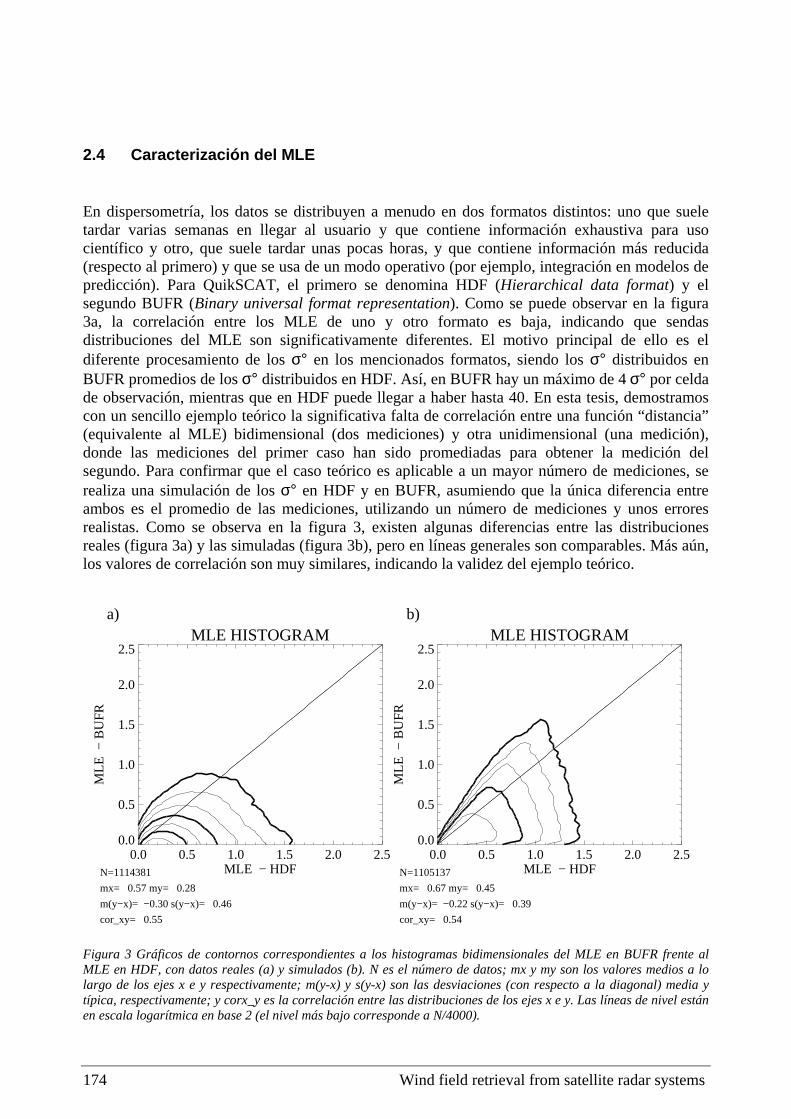
174 Wind field retrieval from satellite radar systems
2.4 Caracterización del MLE
En dispersometría, los datos se distribuyen a menudo en dos formatos distintos: uno que suele tardar varias semanas en llegar al usuario y que contiene información exhaustiva para uso científico y otro, que suele tardar unas pocas horas, y que contiene información más reducida (respecto al primero) y que se usa de un modo operativo (por ejemplo, integración en modelos de predicción). Para QuikSCAT, el primero se denomina HDF (Hierarchical data format) y el segundo BUFR (Binary universal format representation). Como se puede observar en la figura 3a, la correlación entre los MLE de uno y otro formato es baja, indicando que sendas distribuciones del MLE son significativamente diferentes. El motivo principal de ello es el diferente procesamiento de los σ° en los mencionados formatos, siendo los σ° distribuidos en BUFR promedios de los σ° distribuidos en HDF. Así, en BUFR hay un máximo de 4 σ° por celda de observación, mientras que en HDF puede llegar a haber hasta 40. En esta tesis, demostramos con un sencillo ejemplo teórico la significativa falta de correlación entre una función “distancia” (equivalente al MLE) bidimensional (dos mediciones) y otra unidimensional (una medición), donde las mediciones del primer caso han sido promediadas para obtener la medición del segundo. Para confirmar que el caso teórico es aplicable a un mayor número de mediciones, se realiza una simulación de los σ° en HDF y en BUFR, asumiendo que la única diferencia entre ambos es el promedio de las mediciones, utilizando un número de mediciones y unos errores realistas. Como se observa en la figura 3, existen algunas diferencias entre las distribuciones reales (figura 3a) y las simuladas (figura 3b), pero en líneas generales son comparables. Más aún, los valores de correlación son muy similares, indicando la validez del ejemplo teórico.
a) b)
MLE HISTOGRAM
0.0 0.5 1.0 1.5 2.0 2.5MLE − HDF
0.0
0.5
1.0
1.5
2.0
2.5
MLE
− B
UF
R
N=1114381
mx= 0.57 my= 0.28
m(y−x)= −0.30 s(y−x)= 0.46
cor_xy= 0.55
MLE HISTOGRAM
0.0 0.5 1.0 1.5 2.0 2.5MLE − HDF
0.0
0.5
1.0
1.5
2.0
2.5
MLE
− B
UF
R
N=1105137
mx= 0.67 my= 0.45
m(y−x)= −0.22 s(y−x)= 0.39
cor_xy= 0.54
Figura 3 Gráficos de contornos correspondientes a los histogramas bidimensionales del MLE en BUFR frente al MLE en HDF, con datos reales (a) y simulados (b). N es el número de datos; mx y my son los valores medios a lo largo de los ejes x e y respectivamente; m(y-x) y s(y-x) son las desviaciones (con respecto a la diagonal) media y típica, respectivamente; y corx_y es la correlación entre las distribuciones de los ejes x e y. Las líneas de nivel están en escala logarítmica en base 2 (el nivel más bajo corresponde a N/4000).

Resumen (Summary in Spanish) 175
Pese a la poca correlación entre las distribuciones de MLE de ambos formatos (HDF y BUFR), en esta tesis se demuestra que tanto la calidad de los vientos observados como la eficiencia de los controles de calidad en HDF y en BUFR son comparables. Así pues, se concluye que la reducción de la información contenida en las observaciones en BUFR respecto a las observaciones en HDF no es significativa y por tanto no afecta al proceso de obtención del viento.
3 Obtención del viento en sistemas determinados
Como ya hemos visto en la sección 1.4, QuikSCAT es el dispersómetro más adecuado para estudiar los distintos problemas de inversión del viento que plantean las distintas geometrías relativas de los haces del radar. El caso más interesante, por el hecho de ser inédito, es el que plantea la región nadir de QuikSCAT, donde la escasa diversidad azimutal es la causante de la poca precisión de los vientos obtenidos mediante el procedimiento estándar. Las regiones exterior y óptima, en cambio, no presentan problemas significativos de imprecisión y el tipo de geometría que presentan tiene precedentes (instrumentos como el SASS embarcado en Seasat, los SCAT embarcados en ERS-1 y ERS-2 o el NSCAT en ADEOS-1) y por tanto ha sido ampliamente estudiado y optimizado en el pasado.
En este capítulo, describiremos el procedimiento de extracción estándar utilizado en dispersometría y lo aplicaremos a los datos QuikSCAT. Además, propondremos un procedimiento alternativo para mejorar la calidad de las extracciones, especialmente en la región nadir de QuikSCAT. Ambos procedimientos serán validados y comparados con la ayuda de información independiente procedente de un modelo de predicción.
3.1 Procedimiento estándar
Como hemos explicado en la sección 1.4, el procedimiento de extracción del viento consiste primero en invertir las mediciones y posteriormente eliminar la ambigüedad de las soluciones aportadas por la inversión. La inversión, basada en el MLE (ver sección 2.1), se implementa en la práctica con el cálculo de la función coste (ver seción 2.2). En el procedimiento estándar, los mínimos de la función coste representan las soluciones ambiguas del viento posteriormente utilizadas en el proceso de eliminación de la ambigüedad.
Como paso previo a la eliminación de la ambigüedad, los valores del MLE de las soluciones suelen convertirse en valores de probabilidad de ser el viento “verdadero”. La relación entre ésta y el MLE puede inferirse de las ecuaciones (2) y (3) y es la siguiente:
2/1)|( MLEo e
kvp −=σ , (5)
donde v representa el viento “verdadero”, σo el conjunto de las mediciones y k un factor de normalización de la probabilidad (constante). Esta relación teórica puede sufrir en la práctica ligeras variaciones, entre otros motivos, por el comportamiento no uniforme del MLE comentado

176 Wind field retrieval from satellite radar systems
en la sección 2.3. Así pues, en esta tesis, implementamos el método empírico desarrollado por Stoffelen et al. (2000) para encontrar la mencionada relación en los datos QuikSCAT. El Rn es utilizado en la ecuación (5) en lugar del MLE por ser un parámetro más estable (ver sección 2.3). La relación empíricamente determinada entre la probabilidad y el Rn es una exponencial del mismo tipo que la ecuación (5) cuyo exponente tiene como denominador 1.4 (en lugar de 2).
Existen dos procedimientos generalmente utilizados en la eliminación de la ambigüedad. El primero consiste en pasar un filtro medio (JPL, 2001) por un campo de viento que ha sido inicializado con una de las dos soluciones más probables (la más cercana al viento dado por un modelo de predicción que se utiliza como referencia) en cada celda de observación invertida. En este procedimiento, la probabilidad se utiliza de un modo implícito en la inicialización y posteriormente en el filtrado, pero nunca de un modo explícito. El segundo procedimiento es el análisis variacional, método generalmente utilizado en la integración de observaciones en modelos de predicción numéricos. Éste consiste en combinar información de fondo (generalmente de un modelo de predicción) con las mediciones, asumiendo que ambas fuentes de observación tienen errores y éstos están bien caracterizados, para obtener un análisis (campo de viento) consistente espacial y meteorológicamente. Este análisis es utilizado para eliminar la ambigüedad, seleccionando la solución más próxima al análisis en cada celda de observación. En este procedimiento, la probabilidad de cada solución no sólo es utilizada explícitamente sino que además juega un papel muy importante en la eliminación de la ambigüedad.
3.2 Procedimiento de solución múltiple
La obtención del viento por el procedimiento estándar en la región nadir de QuikSCAT es substancialmente imprecisa (ver sección 2.2). El motivo principal es que únicamente los mínimos de la función coste son considerados como soluciones ambiguas. En la región nadir, la función coste presenta mínimos poco definidos (anchos), de modo que la elección del punto mínimo como única solución posible, descartando todos los puntos de alrededor cuya probabilidad de ser el viento “verdadero” es comparable a la del mínimo, no parece apropiada. Si, por el contrario, seleccionamos estos puntos como soluciones ambiguas, estaremos transfiriendo una información más realista al proceso de eliminación de ambigüedad.
Existe un procedimiento de solución múltiple (no limitado a cuatro soluciones o mínimos como el estándar) desarrollado por Stiles et al. (2000). El problema de este método es que usa un filtro medio para eliminar la ambigüedad. Como ya se ha mencionado en la sección 3.1, el filtro medio no utiliza explícitamente el valor de la probabilidad de las soluciones ambiguas. Como consecuencia de ello los campos de viento resultantes a menudo presentan poco variabilidad (más cerca de la variabilidad de los campos de viento de un modelo de mesoescala que de un dispersómetro) y son poco realistas.
En esta tesis, proponemos una alternativa que consiste en utilizar un procedimiento de solución múltiple en combinación con un análisis variacional. Puesto que el análisis variacional está condicionado siempre al balance meteorológico, podemos asegurar que este método producirá vientos realistas.

Resumen (Summary in Spanish) 177
3.3 Comparación entre los procedimientos estándar y de solución múltiple
Tanto el procediminento estándar (PE) como el de solución múltiple (PSM) utilizan el análisis variacional para la eliminación de la ambigüedad. Los términos observacional y de fondo del análisis variacional están representados por las observaciones QuikSCAT (esto es, la información sobre las soluciones ambiguas dadas por cada uno de los procedimientos) y las salidas (esto es, viento en superficie) del modelo NCEP, respectivamente. En la comparación se utilizan las salidas del modelo de predicción del centro europeo de predicción a plazo medio (ECMWF) como referencia.
Los resultados muestran que los vientos PSM son más precisos (esto es, parecidos a ECMWF) que los PE, tanto en la región óptima como en la región nadir. En esta última, la mejora es significativa y se produce en gran parte por la mejora en la calidad de la dirección del viento. Éste es un resultado esperado, puesto que en la región nadir, el PSM permite un número mayor (respecto al PE) de soluciones que se caracterizan por valores similares en módulo y dispares en dirección. Así pues, la probabilidad de encontrar una solución alineada con el flujo “verdadero” es mayor en el PSM que en el PE.
Otro resultado destacado es que la calidad de los vientos del modelo NCEP es menor que la de los vientos tanto del PSM como del PE. De ello se deduce que el análisis variacional asigna un peso mayor a las observaciones (mediciones de QuikSCAT) que a la información de fondo (NCEP). De este modo, los métodos de obtención del viento (PE y PSM) no depeden de forma significativa de la calidad de la información de fondo. Esto es muy importante puesto que se trata de obtener campos de viento de la forma más independiente (basados en las observaciones radar).
a) b)
Figura 4 Campos de viento del PE (a) y del PSM (b). La fecha de adquisición es el 3 de Febrero de 2002 a las 2 horas UTC. Las lineas sólidas separan las distintas regiones del campo de observación de QuikSCAT: región óptima derecha (parte izquierda), región nadir (parte central) y región ótptima izquierda (parte derecha).

178 Wind field retrieval from satellite radar systems
La figura 4 muestra las diferencias entre el PE y el PSM. El campo de viento del PE (figura 4a) es sustancialmente inconsistente en la región nadir. Por el contrario, el campo de viento del PSM (figura 4b) es espacialmente consistente tanto en la región nadir como en la óptima. Así pues, el PSM es capaz de filtrar el “ruido” que hay en el viento del PE manteniendo al mismo tiempo la información dinámica existente (la intensidad y la posición de la borrasca son iguales en las dos figuras).
En esta tesis, se han examinado un gran número de casos meteorológico. En general, el PSM produce campos de viento más consistentes y realistas que el PE, especialmente en la región nadir. Así pues, los vientos PSM resultan particularmente interesantes en el campo de la integración de datos en modelos de mesoescala como ECMWF.
4 Obtención del viento en sistemas indeterminados
Los sistemas radar con un solo haz o visión en principio presentan un problema de indeterminación a la hora de invertir el vector viento (ver sección 1.4). En este sentido, el SAR es pues el sistema adecuado para estudiar este tipo de problemas puesto que sólo dispone de un haz lateral de visión fija. Como hemos visto en los capítulos precedentes, el MLE es un parámetro válido para la inversión en problemas determinados. Sin embargo, es obvio que en caso de indeterminación se necesitará información adicional para invertir el vector viento. Esta información adicional puede a veces extraerse de las propias imágenes SAR y/o de modelos de predicción o boyas. En este capítulo compararemos dos métodos de obtención del viento. El primero, habitualmente utilizado, supone que el SAR es un sistema determinado y por tanto capaz de extraer el vector viento de un modo independiente. El segundo, propuesto en esta tesis como alternativa al primero, supone que el SAR es un sistema indeterminado y está basado en un método estadístico que combina las informaciones del SAR y de un modelo de predicción para obtener el vector viento.
4.1 Algoritmos de obtención del viento para SAR
Hoy en día existen tres algoritmos comúnmente utilizados en la obtención del viento a partir de imágenes SAR: el modelo CMOD-4, el SWDA (SAR wind direction algorithm) y el SWA (SAR wind algorithm).
El CMOD-4 es la GMF (ver ecuación 1) más utilizada en la inversión del viento a partir de datos del dispersómetro SCAT de los satélites ERS. El problema de la inversión en SAR es que su único haz es sensible tanto a la dirección como al módulo del viento (dos incógnitas), lo cual conlleva problemas de ambigüedad e indeterminación.
El SWDA es un algoritmo de obtención de la dirección del viento. Está basado en la detección de expresiones lineales (sobre el mar) en la imagen SAR, que a menudo están asociadas con wind streaks o wind rows. Estos últimos son manifestaciones (en la imagen) de vórtices circulares que se forman en la capa límite planetaria y que están aproximadamente alineados con el viento local.

Resumen (Summary in Spanish) 179
El SWA es un algoritmo de obtención del módulo del viento. Está basado en la detección de las olas más grandes a partir del espectro de la imagen SAR. Estas olas, al estar en equilibrio con el viento local, nos dan información sobre el módulo del viento en superficie. El equilibrio de las olas con el viento local se rompe en aguas poco profundas, dando lugar a errores significativos en la estimación del viento por parte del SWA. Como las imágenes SAR utilizadas en esta tesis están localizadas en aguas poco profundas, el SWA será descartado y nos centraremos en el CMOD-4 y el SWDA.
4.2 Método estadístico
Al margen de las limitaciones de los algoritmos presentados en la sección anterior, hay un problema importante que es inherente al sistema de observación SAR. Tanto la dirección como el módulo del viento están presentes al mismo tiempo y no pueden distinguirse del todo. Así pues, un método que combine estos algoritmos con información adicional externa podría ser la solución a este problema. Para ello, el método tendría que tener en cuenta las características espaciales, las limitaciones y la precisión de todas las fuentes de información.
En esta sección, presentamos un método estadístico utilizado por Lorenc (1986) para resolver problemas de inversión en análisis meteorológico. Está basado en el método Bayesiano presentado en la sección 2.1. La diferencia es que en lugar de considerar la probabilidad a priori de A (vector viento) como constante, en este caso se utiliza la información de fondo de una fuente externa para caracterizar la mencionada probabilidad, de modo que la ecuación (2) se puede escribir ahora de la siguiente forma:
)]()(2
1)}({)()}({
2
1exp[)( 11
bboo xxBxxxyFOxyx −−−−+−−∝ −− Tn
Tna kkP (6)
donde xb es la información de fondo del campo de viento (por ejemplo, las salidas de un modelo de predicción), y B representa la matriz de covarianza o errores de la información de fondo. Del mismo modo que para la ecuación (2), maximizar la probabilidad de obtener el viento “verdadero” (Pa(x)) es equivalente a minimizar los dos términos del exponente de la ecuación (2), también denominados términos observacional (el primero) y de fondo (el segundo).
4.3 Evaluación de dos métodos de obtención del viento para SAR
En esta sección, se evalúan dos métodos diferentes de obtención del viento de alta resolución (5 km) a partir de imágenes SAR. El primero, generalmente utilizado para SAR, está basado en la combinación de los algoritmos SWDA y CMOD-4. El segundo es un método nuevo basado en el método estadístico presentado en la sección 4.2 y llamado SWRA (SAR wind retrieval algorithm). En esta evaluación se utilizan 15 imágenes SAR y las salidas de muy alta resolución (VHR, Very-high resolution) del modelo de predicción HIRLAM (High resolution limited area model).

180 Wind field retrieval from satellite radar systems
Método SWDA+CMOD-4
El método consiste en extraer primero la información sobre la dirección del viento con el algoritmo SWDA. Con esta información, se puede invertir directamente el módulo del viento utilizando CMOD-4 (ver ecuación 1). De este modo, se puede obtener el vector viento de un modo independiente, es decir, sin utilizar información adicional.
La evaluación de este método revela sin embargo varios problemas. En primer lugar, el SWDA detecta la dirección del viento con una resolución no mayor de 25 km. Así, toda la variabilidad entre 25 km y 5 km es asignada (erróneamente) al módulo del viento. Además, el SWDA no siempre detecta wind streaks y estos últimos en cualquier caso no están perfectamente alineados con el viento, añadiendo más incertidumbre a la medición del viento. Es importante destacar también que la precisión del SWDA disminuye con la distancia entre wind streaks. Por último, el problema más importante es que el método asume los algoritmos como perfectos, de modo que los errores en la estimación del módulo del viento (CMOD-4) están directamente afectados por los errores en la estimación de la dirección (SWDA).
Método SWRA
El SWRA consiste en aplicar el método estadístico al caso del SAR, utilizando asunciones simples. Así, si utilizamos el modelo CMOD-4 como GMF, el VHR como información de fondo, y asumimos que no hay correlación espacial de los errores (O+F y B son matrices diagonales), el exponente de la ecuación (6) se puede escribir ahora como:
222
∆−
+
∆−
+
∆−
=v
vv
u
uuJ HH
oom
σσσ
(7)
donde σmo es el coeficiente de retrodispersión del SAR para una celda de observación
determinada; uH y vH son las componentes del vector viento “observado” por el VHR; ∆σ, ∆u y ∆v son los errores gaussianos de las matrices de covarianza obtenidos empíricamente; u y v son las componentes del vector viento que buscamos (o sea, que minimice el coste J) y σo es el valor del coeficiente de retrodispersión correspondiente al vector viento (u,v) y determinado por CMOD-4 (ver ecuación 1). El primer término de la ecuación (7) se denomina término SAR y los otros dos se denominan término VHR.
A diferencia del método anterior, el SWRA garantiza la obtención de un campo de viento y no considera las fuentes de información como perfectas (exentas de errores). Éste método permite extraer el campo de viento óptimo, producto de la mejor combinación de las informaciones del SAR y del VHR. En este sentido, el SWRA resulta muy prometedor. Sin embargo, la variabilidad del viento resultante (básicamente aportada por la información SAR) está distribuida de una forma predefinida entre el módulo y la dirección, de acuerdo con las respectivas sensibilidades del modelo CMOD-4. Como se observa en la tabla 1, la variabilidad del viento del SWRA es un compromiso entre las variabilidades del VHR y del SAR para el módulo del viento. Sin embargo, no ocurre lo mismo con la dirección. Esto es debido a que generalmente CMOD-4 tiene mayor sensibilidad (más del doble) a cambios en el módulo que en la dirección. Para evitar que la dirección resultante esté demasiado dominada por el término VHR, se recomienda añadir

Resumen (Summary in Spanish) 181
información sobre detección de wind streaks (SWDA) en el término SAR, tras una exhaustiva caracterización de los errores y la precisión del SWDA.
5 Control de calidad
El control de calidad (CC) de las extracciones de campos de viento a partir de datos radar es de una gran importancia en aplicaciones como la integración de datos en modelos de predicción. Para lograr establecer un CC eficiente, el MLE resulta ser un parámetro muy útil.
Como ya hemos mencionado en la sección 2.1, el MLE se puede interpretar como una medida de la distancia entre las mediciones y la solución que yace en la GMF. El MLE por tanto indica en qué medida las mediciones se ajustan a la GMF cuya superficie se ha calculado empíricamente con distintas condiciones de viento. Así pues, inconsistencias entre las mediciones y la GMF dan como resultado valores altos de MLE, indicando por tanto condiciones geofísicas distintas a las modeladas por la GMF como la lluvia, el estado de mar ambiguo o el hielo marino. De este modo, el MLE nos da una buena indicación de la calidad de las extracciones del viento.
En este capítulo, nos centraremos en establecer un procedimiento de CC basado en el MLE. Este mismo principio se ha utilizado en el pasado para establecer el CC de radares como SCAT o NSCAT. Sin embargo, no existe todavía un CC para QuikSCAT cuyo problema con la lluvia hace del CC un elemento indispensable para la obtención de vientos de buena calidad. Es más, en la actualidad, no existe ningún método genérico de CC aplicable a cualquier radar. Así pues, en esta tesis desarrollaremos un método de CC genérico, a partir de los datos QuikSCAT. Dado que existe un método de detección de lluvia desarrollado por el JPL (Jet propulsion Laboratory) para datos QuikSCAT, en la segunda parte de este capítulo efectuaremos una comparación de nuestro CC, desarrollado en el KNMI (Instituto Meteorológico Holandés), con el mencionado método del JPL con el fin de mejorar el control de calidad, en este caso, de QuikSCAT.
5.1 Procedimiento genérico de CC
El procedimiento basado en el MLE que presentaremos a continuación utiliza el Rn como indicador de la calidad de las extracciones (en lugar del MLE), puesto que es un parámetro
Tabla 1. Comparación de la variabilidad.
Componentes del viento Variabilidad en VHR
Variabilidad en SWRA
Variabilidad en SAR
Módulo (m/s) 0.55 0.75 1
Dirección (m/s)1 0.45 0.45 1.65 1 Los valores de la dirección están dados en m/s equivalentes, es decir, teniendo en cuenta la intensidad del viento en la cuantificación del error en la dirección.

182 Wind field retrieval from satellite radar systems
sensiblemente más estable que el MLE (ver sección 2.3). De acuerdo con la relación entre el Rn y el MLE (ver ecuación 4), cuando la retrodispersión de una celda de observación está “contaminada” por otros efectos geofísicos que no sean el viento, el Rn tendrá valores altos; en cambio, cuando la retrodispersión está dominada por el efecto geofísico del viento, el Rn tendrá valores cercanos a la unidad. Así pues, el método consiste en la determinación empírica de un umbral de Rn que separe los vientos de buena calidad de los de mala calidad. Para ello, se utilizarán co-localizaciones de datos QuikSCAT con los campos de viento del modelo de ECMWF y las observaciones de lluvia obtenidas por el SSM/I (Special sensor microwave imager) embarcado en el satélite DMSP (Defense meteorological satellite program).
Como paso previo a la determinación del umbral, caracterizamos el Rn o, en otras palabras, examinamos la relación entre el Rn y la calidad de las extracciones para determinar la existencia del mencionado umbral. Los resultados muestran una clara correlación entre la calidad de las extracciones y el valor de Rn. La calidad disminuye a medida que el Rn aumenta, siendo el ritmo de tal disminución mayor cuanto más fuerte sea el viento. La presencia de lluvia incrementa artificialmente el valor del módulo del viento obtenido. Para cantidades de lluvia superiores a 6 mm/hora, la información predominante en la señal (retrodispersión) no es el viento sino la lluvia, que a su vez produce unos (falsos) vientos de 15-20 m/s en el proceso de extracción.
A continuación, se define un umbral que depende del módulo del viento obtenido. El umbral se ajusta en un proceso de validación que consiste en utilizar las co-localizaciones mencionadas anteriormente para determinar la calidad de los datos aceptados (con valor de Rn inferior o igual al umbral definido) y rechazados (con valor de Rn superior al umbral) por nuestro CC. El umbral óptimo en términos de rechazo mayoritario de datos de baja calidad y aceptación mayoritaria de datos de buena calidad es el siguiente:
,5,100
2,4
,
2/15
)(/15
00
200
=−==
=⇒>−⋅+=⇒≤
vAy
donde
ysmv
vvAyysmv
(8)
v es el módulo del viento obtenido e y el valor umbral de Rn.
Los resultados de la validación muestran que, para el umbral definido en la ecuación (8), el 97% de los datos de buena calidad son aceptados, la calidad de los datos rechazados es muy baja con respeto a la calidad de los datos aceptados y la mayoría de las celdas de observación “contaminadas” por lluvia son rechazadas por nuestro CC.
Los resultados de aplicar el CC en datos QuikSCAT se pueden ver en la figura 5. Ésta muestra los campos de viento co-localizados de QuikSCAT (figura 5a) y de EMWF (figura 5b) para una situación meteorológica determinada. En la parte central del campo de viento hay un frente bien definido donde generalmente el estado del mar es ambiguo y por tanto la calidad de las extracciones es baja. Como se puede observar, a lo largo del frente, el CC ha rechazado la mayoría de las celdas de observación (flechas rojas). Lo mismo ocurre en las proximidades del centro de bajas presiones situado en la parte baja del gráfico, donde probablemente hay una alta variabilidad temporal y espacial del estado del mar. La parte izquierda del frente presenta una región sensiblemente afectada por la de lluvia (valores superiores a 6 mm/hora), como lo indican

Resumen (Summary in Spanish) 183
los datos SSM/I co-localizados (ver cuadrados), que ha sido detectada por el CC (ver flechas rojas).
Las implicaciones de un CC eficiente como el presentado aquí quedan patentes en este caso meteorológico. Como se observa al comparar la figuras 5a y 5b, las predicciones de ECMWF han errado significativamente en la localización del centro de bajas presiones y de su frente asociado. Así pues, el impacto potencialmente positivo de integrar los datos QuikSCAT en modelos de predicción como ECMWF después de aplicar este CC queda claramente ilustrado con este ejemplo.
5.2 Comparación entre los procedimientos de CC del KNMI y de detección de lluvia del JPL
Como se ha visto en la sección precedente, la detección de la lluvia es de gran importancia para el CC de los datos QuikSCAT. En este sentido, el JPL ha desarrollado un procedimiento de
CASO : 02/09/99 1400 UTC
a) b)
Figura 5 Co-localizaciones de datos QuikSCAT, ECMWF y SSM/I. El gráfico (a) muestra el campo de viento obtenido a partir de datos QuikSCAT, donde las flechas de color gris corresponden a los vientos aceptados por el CC y las de color negro a los vientos rechazados por el CC. El tamaño de los cuadrados representa la cantidad de lluvia observada por el SSM/I, desde 0 mm/hora (no hay cuadrado) hasta 25 mm/hora (los cuadrados más grandes). El gráfico (b) muestra el campo de viento co-localizado dado por ECMWF. Las líneas sólidas separan las distintas partes del campo de observación: la parte izquierda del gráfico corresponde a la región nadir, la central a la región óptima y la parte derecha a la región exterior. Las observaciones fueron adquiridas el 2 de Septiembre de 1999 a las 14 horas UTC.

184 Wind field retrieval from satellite radar systems
detección de lluvia para QuikSCAT. Este método está basado en una serie de parámetros que son identificados como sensibles a la lluvia. Estos parámetros son, entre otros, la diferencia normalizada entre las retrodispersiones de los distintos haces, el módulo y la dirección del viento obtenido y el MLE.
Con el fin de mejorar el CC para QuikSCAT, se realiza una comparación del CC propuesto en la sección precedente con el método de detección de lluvia del JPL. Para ello se utilizarán de nuevo datos ECMWF y SSM/I co-localizados. La comparación se realiza en las regiones nadir y óptima.
Los resultados muestran que el CC del KNMI detecta (rechaza) un 4% de datos que son de mala calidad y en su mayoría no contaminados por la lluvia y que no han sido detectados por el método del JPL. Éste, por su parte, detecta un 2% de datos de mala calidad y parcialmente contaminados por la lluvia y que no han sido detectados por el CC del KNMI. De este modo, el CC es más eficiente como indicador de calidad (en general) mientras que el método del JPL es más eficiente como indicador de lluvia.
El CC del KNMI está basado en el MLE, que resulta ser un buen parámetro para el CC. El método del JPL está basado no sólo en el MLE sino también en otros parámetros, que son identificados como sensibles a la lluvia como ya hemos mencionado anteriormente. Sin embargo, estos otros parámetros no están relacionados con la calidad de los datos, lo cual explica por qué el CC del KNMI funciona mejor como indicador de calidad.
Aun así, se puede apreciar que hay una parte considerable de datos de mala calidad, parcialmente contaminados por la lluvia, que son detectados por el método del JPL y no por el CC del KNMI, sugiriendo que ambos métodos son complementarios y que su combinación podría mejorar sensiblemente el CC de QuikSCAT. Sin embargo, los resultados también muestran que el método del JPL tiende a rechazar muchos datos en zonas dinámicamente activas y no contaminadas por la lluvia.
La calidad de los datos se determina por comparación con los datos del modelo ECMWF. En las zonas dinámicamente activas, es precisamente donde se espera que los modelos de predicción sean más imprecisos y por tanto donde las estadísticas sobre la calidad de los datos puedan ser menos fiables. De modo que es necesario recurrir al examen directo de situaciones meteorológicas para determinar si la calidad de estos datos rechazados por el JPL es realmente mala.
Después de examinar numerosos campos de viento, se observa que en la región óptima de QuikSCAT, hay un exceso de vientos fuertes, espacial y meteorológicamente consistentes, que son rechazados por el método del JPL. En la región nadir, donde la eficiencia del CC del KNMI es menor comparada con la eficiencia en la región óptima, el método del JPL es capaz de detectar algunos vientos de mala calidad, contaminados por la lluvia, que no son detectados por el CC del KNMI.
Así pues, se recomienda el uso del CC del KNMI para los datos QuikSCAT. En la región óptima, el CC del KNMI es suficiente; sin embargo, en la región nadir, se recomienda el uso combinado del CC del KNMI y el método de detección de lluvia del JPL.

Acronyms 185
Acronyms
2D-Var Two-dimensional Variational Analysis 3D-Var Three-dimensional Variational Analysis 4D-Var Four-dimensional Variational Analysis ADEOS Advanced Earth Observation Satellite AER Atmospheric Environmental Research Inc. AMSR Advanced Microwave Scanning Radiometer AR Ambiguity Removal ASAR Advanced SAR ASCAT Advanced Scatterometer ATSR Along Track Scanning Radiometer BUFR Binary Universal Format Representation CERSAT Centre ERS d’Archivage et de Traitement CDTI Centro para el Desarrollo Tecnológico e Industrial CMOD-4 ESA C-band GMF for the ERS Scatterometer CMOD-Ifr Ifremer C-band GMF for the ERS Scatterometer DIR Direction Interval Retrieval DIRTH DIR + TN DMSP Defense Meteorological Satellite Program DNMI Norwegian Meteorological Institute DoD Department of Defense (USA) DWL Doppler Wind Lidar ECMWF European Centre for Medium-range Weather Forecasts EM Electromagnetic ENSO El Niño Southern Oscillation ENVISAT Environmental Satellite ERS European Remote Sensing Satellite ESA European Space Agency ESRIN European Space Research Institute ESTEC European Space Research and Technology Centre EUMETSAT European Meteorological Satellite Organization GA General Approach GMF Geophysical Model Function GOMOS Global Ozone Monitoring by Occultation of Stars GOS Global Observing System GPS Global Positioning System GTS Global Telecommunication System

186 Wind field retrieval from satellite radar systems
HDF Hierarchical Data Format HIRLAM High-Resolution Limited Area Model HIRS High-Resolution Infrared Radiation Sounder H-pol Horizontal Polarization IFREMER Institut Français de Recherche pour l’Exploitation de la Mer. JERS Japanese Earth Resources Satellite JPL Jet Propulsion Laboratory KNMI Royal Netherlands Meteorological Institute LOS Line of Sight LUT Look-up-table MBL Marine Boundary Layer MEC Ministerio de Educación y Ciencia METOP Meteorological Operational Polar Satellites MLE Maximum Likelihood Estimator <MLE> Expected MLE MSS Multiple Solution Scheme MUDH Multidimensional Histogram NASA National Air and Space Administration (USA) NCEP National Centre for Atmospheric Prediction (USA) NOAA National Oceanographic and Atmospheric Administration (USA) NRMS Normalized RMS in wind direction NRCS Normalized Radar Cross Section NRT Near Real Time NSCAT NASA Scatterometer NSCAT-2 NASA Ku-band GMF for NSCAT NWP Numerical Weather Prediction OVWST Ocean Vector Wind Science Team PBL Planetary Boundary Layer PDF Probability Density Function PRI Precision Image QC Quality Control QSCAT-1 NASA Ku-band GMF for QuikSCAT QuikSCAT NASA satellite dedicated the first SeaWinds instrument RAR Real Aperture Radar RFSCAT Rotating Fan-beam Scatterometer RMS Root-Mean-Squared RMS-ECMWF Mean RMS of vector difference between JPL-selected and ECMWF winds Rn Normalized Residual RR Rain Rate SAF Satellite Application Facility SAG Science Advisory Group SAR Synthetic Aperture Radar SASS Seasat-A Scatterometer System Seasat Sea State Satellite SeaWinds NASA Ku-band rotating pencil-beam scatterometer SD Standard Deviation SLC Single-look complex SSM/I Special Sensor Microwave Imager SWA SAR Wind Algorithm SWDA SAR Wind Direction Algorithm

Acronyms 187
SWRA Statistical Wind Retrieval Approach SWT Science Working Team TN Thresholded Nudging UKMO United Kingdom Meteorological Office USA United States of America UTC Universal Time Coordinated V55 Operational (55 km resolution) HIRLAM VHR Very High Resolution HIRLAM V-pol Vertical Polarization WVC Wind Vector Cell WMO World Meteorological Organization

188 Wind field retrieval from satellite radar systems

Bibliography 189
Bibliography
Alpers, W., and Brummer, B., “Atmospheric boundary layer rolls observed by the synthetic aperture radar aboard the ERS-1 satellite,” J. Geophys. Res., vol. 99, no. C6, pp. 12613- 12621, 1994.
Alpers, W., “Measurement of mesoscale oceanic and atmospheric phenomena by ERS-1 SAR,” Radio Sci. Bull. 275, pp. 14-22, Int. Union of Radio Sci., c/o University of Gent (INTEC), Gent, Belgium, 1995.
Alpers, W., Pahl, U., and Gross, G., “Katabatic wind fields in coastal areas studied by ERS-1 synthetic aperture radar imagery and numerical modelling,” J. Geophys. Res., vol. 103, no. C4, pp. 7875-7886, 1998.
Atlas, R, and Hoffman, R.N., “The use of satellite surface wind data to improve weather analysis and forecasting at the NASA data assimilation office,” Satellites, Oceanography and Society, D. Halpern, ed. Elsevier Science B.V., pp. 57-78, 2000.
Atlas, R., Hoffman, R.N., Leidner, S.M, Sienkiewicz, J., Yu, T.-W., Bloom, S.C., Brin, E., Ardizzone, J., Terry, J., Bungato, D., Jusem, J.C., “The effects of marine winds from scatterometer data on weather analysis and forecasting,” Bull. Amer. Meteorol. Soc., vol. 82, no. 9, pp. 1965-1990, 2001.
Bentamy, A., Quilfen, Y., and Flament, P., “Scatterometer wind fields – a new release over the decade 1991-2001,” Can. Jour. of Rem. Sens., vol. 28, no. 3, 2002.
Boukabara, S.A., Hoffman, R.N., and Grassotti, C., “Atmospheric compensation and heavy rain detection for SeaWinds using AMSR,” Atmospheric Environmental Research Inc., 1999.
Brown, R.A., “Surface fluxes and remote sensing of air-sea interactions, surface waves and fluxes,” eds. G.L. Geernaert and W.J. Plant, Kluwer Academic Publishers, Dordrecht, The Netherlands, pp. 7-27, 1990.
Cavanié, A., “Evaluation of Kp on central and lateral antennas of NSCAT over artic sea ice,” Report presented at the 12th ASCAT Science Advisory Group Meeting, Darmstadt, Germany, 16-17 October 1997.
Chapron, B., Fouhaily, T. E., and Kerbaol, V., “Calibration and validation of ERS wave mode products,” Document DRO/OS/95-02, Institut Français de Recherche pour l’Exploitation de la Mer, 1995.
190 Wind field retrieval from satellite radar systems
De Bruijn, E. I. F., “Experiments with horizontal diffusion and advection in a nested fine mesh mesoscale model,” Scientific report WR-97-08, Koninklijk Nederlands Meteorologisch Instituut (KNMI), De Bilt, The Netherlands, 1997.
De Bruijn, E. I. F., and Brandsma, T., “Rainfall prediction for a flooding event in Ireland caused by the remnants of hurricane Charley,” Journal of Hydrology, vol. 239, pp. 148-161, 2000.
Doneland, M.A., Dobson, F.W., Smith, S.D., and Anderson, R.J., “On the dependence of sea surface roughness on wave development,” J. Physical Oceanography, vol. 23, pp. 2143-2149, 1993.
EOQ - Earth Observation Quarterly, European Space Agency Publications Division, ESTEC, postbus 299, 2200 AG Noordwijk, The Netherlands, no. 59, 1998.
Etling, D., and Brown, R. A., “Roll vortices in the planetary boundary layer: a review,” Boundary Layer Meteorol., vol. 65, pp. 215-248, 1993.
ESA, “ERS user handbook,” revision 1, European Space Agency SP-1148, September 1993.
Figa, J., and Stoffelen, A., “On the assimilation of Ku-band scatterometer winds for weather analysis and forecasting”, IEEE Trans. on Geoscience and Rem. Sens., vol. 38 (4) pp. 1893-1902, July 2000.
Figa-Saldana, J., Wilson, J.J.W., Attema, E., Gelsthorpe, R., Drinkwater, M.R., and Stoffelen, A., “The advanced scatterometer (ASCAT) on METOP: a follow-on for European scatterometers,” Can. Jour. of Rem. Sens., vol. 28, no. 3, 2002.
Fetterer, F., Gineris, D., and Wackerman, C., “Validating a scatterometer wind algorithm for ERS-1 SAR,” IEEE Trans. Geosci. Rem. Sens., vol. 36, no. 2, 1998.
Freilich, M.H., Vanhoff, B.A., and Dunbar, R.S., “Empirical determination of a Ku-band wind model function from SeaWinds scanning scatterometer,” J. Geophys. Res. (in prep.), 2002.
Garrison, J.L., Katzberg, S.J., Hill, M.I., “Effect of sea roughness on bistatically scattered range coded signals from the Global Positioning System,” Geophys. Res. Lett., vol. 25, no. 13, pp. 2257-2260, 1998.
Gerling, T. W., “Structure of the surface wind field from the Seasat SAR,” J. Geophys. Res., vol. 91, no. C2, pp. 2308-2320, 1986.
Goodman, J.W., “Some fundamental properties of speckle,” J. Optical Soc. of Am., vol. 66, pp.1145-1150, 1976.
Grabak, O., and Laur, H., “ERS SAR.PRI CCT and Exabyte,” Document ER-IS-EPO-GS-5902.4, European Space Agency, Italy, 1995.
Grima, N., Bentamy, A., Katsaros, K., Quilfen, Y., Delecluse, P., and Levy, C., “Sensitivity of an oceanic general circulation model forced by satellite wind stress fields,” J. Geophys. Res., vol 104, C4, pp. 7967-7989, 1999.

Bibliography 191
Gudiksen, P. H., Leone, J. M., King, C. W., Ruffieux, D., and Neff, W. D., “Measurements and modelling of the effects of ambient meteorology on nocturnal drainage flows,” J. Appl. Meteorol., vol. 31, pp. 1023-1032, 1992.
Gustafsson, N., “The HIRLAM model,” Seminar Proceedings on Numerical Methods in Atmospheric Models, vol. 2, pp. 115-146, 1991.
Hasselmann, K., Raney, R.K., Plant, W.J., Alpers, W., Shuchman, R.A., Lyzenga, D.R., Rufenach, C.L., and Tucker, M.J., “Theory of synthetic aperture radar ocean imaging: a MARSEN view,” J. Geophys. Res., vol. 90, no. C3, pp. 4659-4686, 1985.
Huddleston, J.N., and Stiles, B.W., “Multidimensional histogram (MUDH) rain flag”, version 2.1, Jet Propulsion Laboratory, available at http://podaac-www.jpl.nasa.gov/quikscat/, September 2000.
Ifremer, “WNF products - user manual,” Ifremer-Cersat, ref. C2-MUT-W-01-IF, 1996.
Isaksen, L., and Stoffelen, A., “ERS scatterometer wind data impact on ECMWF’s tropical cyclone forecasts” IEEE Trans. on Geoscience and Rem. Sens., vol. 38 (4) pp. 1885-1892, July 2000.
Janssen, P.A.E.M., Wallbrink, H., Calkoen, C.J., van Halsema, D., Oost, W.A., and Snoeij, P., “VIERS-1 scatterometer model,” J. Geophys. Res., vol. 103, no. C4, pp. 7807-7831, 1998.
Johannessen, J. A., Schuchman, R., Johannessen, O. M., Davidson, K., and Lyzenga, D. R., “Synthetic aperture radar imaging of ocean circulation features and wind fronts,” J. Geophys. Res., vol. 96, no. C6, pp. 10411-10422, 1991.
Johannessen, J. A., Vachon, P. W., and Johannessen, O. M., “ERS-1 SAR imaging of marine boundary layer processes,” ESA EOQ no. 46, 1994a.
Johannessen, J.A., Digranes, G., Espedal, H., Johannessen, O.M., Samuel, P., Browne, D., Vachon, P.W., “SAR ocean feature catalogue,” ESA SP-1174, European Space Agency, 1994b.
Johannessen, J. A., Vachon, P. W., and Johannessen, O. M., “ERS-1 SAR imaging of marine boundary layer processes, Study of Earth System from Space,” Journal of Earth Observation and Remote Sensing (Russian), No. 3, 1996.
Johnsen, H., Engen, G., Hogda, K., Chapron, B., and Desnos, Y., “Validation of Envisat ASAR wave mode level 1b and level 2b products using ERS SAR data,” Proc. of CEOS SAR Workshop, ESA SP-450, Toulouse, pp. 59-64, 1999.
Jones, L., Mladen, S., Park, J., and Mehershadi, R., “A Quality Control Rain Flag using QuikSCAT Radiometric Observations,” Proc. of QuikSCAT Cal/Val Workshop, Pasadena/Arcadia (USA), November 1999.
JPL, “QuikSCAT science data product user’s manual”, version 2.2, Jet Propulsion Laboratory D-12985, pp. 89, December 2001.
JPL, “NASA scatterometer science data product user’s manual,” version 1.1, Jet Propulsion Laboratory D-18053, pp. 68, April 1997.
192 Wind field retrieval from satellite radar systems
Kerbaol, V., “Analyse spectrale et statistique vent-vagues des images radar a ouverture synthetique: application aux donnees des satellites ERS-1/2,” PhD thesis at the University of Rennes 1, December 1997.
Kerbaol, V., Chapron, B., and Vachon, P. W., “Analysis of ERS-1/2 synthetic aperture radar wave mode imagettes,” J. Geophys. Res., vol. 103, no. C4, pp. 7833-7846, 1998.
Komen, G.J., Cavaleri, L., Donelan, M., Hasselmann, K., Hasselmann, S., Janssen, P.A.E.M., “Dynamics and modelling of ocean waves,” Cambridge University Press, 1994.
Komjathy, A., Zavorotny, V.U., Axelrad, P., Born, G.H., Garrison, J.L., “GPS signal scattering from sea surface: wind speed retrieval using experimental data and theoretical model,” Remote Sensing of Environment, vol. 73, no. 2, pp. 162-174, 2000.
Korsbakken, E., Johannessen, J. A., and Johannessen, O. M., “Coastal wind field retrievals from ERS synthetic aperture radar images,” J. Geophys. Res., vol. 103, no. C4, pp. 7857- 7874, 1998.
Latif, M., Anderson, D., Barnett, T., Cane, M., Kleeman, R., Leetmaa, A., O’Brien, J., Rosati, A., and Schneider, E., “A review of the predictability and prediction of ENSO,” J. Geophys. Res., vol. 103, no. C7, pp. 14375-14393, 1998.
Laur, H., Bally, P., Meadows, P. J., Sanchez, J., Schaettler, B., and Lopinto, E., “ERS SAR calibration: Derivation of the backscattering coefficient σ° in ESA ERS SAR PRI products,” Document ES-TN-RS-PM-HL09, Issue 2, Rev. 5, European Space Agency, 1998.
Lehner, S., Horstmann, J., Koch, W., and Rosenthal, W., “Mesoscale wind measurements using recalibrated ERS SAR images,” J. Geophys. Res., vol. 103, no. C4, pp. 7847-7856, 1998.
Leidner, M., Hoffman, R., and Augenbaum, J., “SeaWinds scatterometer real-time BUFR geophysical data product”, version 2.2.0, NOAA/NESDIS, February 2000.
LeMone, M.A., “Structure and dynamics of horizontal roll vortices in the Planetary Boundary Layer,” J. Atm. Sci., 30, pp. 1077-1091, 1973.
Lin, C., Stoffelen, A., De Kloe, J., Wismann, V., Bartha, S., Schulte, H., “Wind retrieval capability of rotating, range-gated, fanbeam spaceborne scatterometer,” Proc. of SPIE on Remote Sensing, vol. 4880, Crete, Greece, September 2002.
Lorenc, A.C., “Analysis methods for numerical weather prediction,” Quart. J. R. Met. Soc., vol. 112, pp. 1177-1194, 1986.
Mastenbroek, K., “Wind-wave interaction,” PhD thesis at the Delft University of Technology, Delft, The Netherlands, December 1996.
McNider, R. T., and Pielke, R. A., “Numerical simulation of slope and mountain flows,” J. Appl. Meteorol., vol. 23, 1441-1453, 1984.
Mears, C., Wentz, F., and Smith, D., “SeaWinds on QuikSCAT normalized objective function rain flag,” version 1.2, Jet Propulsion Laboratory, available at http://podaac-www.jpl.nasa.gov/quikscat/, September 2000.

Bibliography 193
Pierson, W.J., “Highlights of the Seasat-SASS program: a review,” Satellite Microwave Remote Sensing, T.D. Allan, ed. Ellis Horwood Ltd., pp. 69-86, 1983.
Pierson, W.J., “Probabilities and statistics for backscatter estimates obtained by a scatterometer,” J. Geophys. Res., vol. 94, no. C7, pp. 9743-9759, 1989.
Plant, W.J., “Relationship between stress wind and wave slope,” J. Geophys. Res., vol. 87, no. C3, pp. 1961-1967, 1982.
Pond, S., and Pickard, G. L., “Introductory dynamic oceanography,” edited by Pergamon Press, 1978.
Portabella, M., “ERS-2 SAR wind retrievals versus HIRLAM output: a two way validation-by-comparison,” ESA report EWP-1990, European Space Research and Technology Centre, Noordwijk, The Netherlands, 1998.
Portabella, M., Stoffelen, A., and De Vries, J., “Development of a SeaWinds wind product for weather forecasting,” Proc. of International Geoscience and Remote Sensing Symposium (IGARSS), vol. III, pp. 1076-1078, 2001.
Portabella, M., and Stoffelen, A., “A probabilistic approach for SeaWinds data assimilation: an improvement in the nadir region,” Visiting Scientist report for the EUMETSAT NWP SAF, available at http://www.eumetsat.de/en/area4/saf/internet/, 2002.
Quilfen, Y., Bentamy, A., Delecluse, P., Katsaros, K.B., and Grima, N., “Prediction of sea level anomalies using ocean circulation model forced by scatterometer wind and validation using TOPEX/Poseidon data,” IEEE Trans. Geosci. Rem. Sens., vol 38, no. 4, pp. 1871-1884, 2000.
Rodgers, C. D., “Inverse methods for atmospheric sounding: theory and practice,” World Scientific Publishing Co., 2000.
Rohn, M., Kelly, G., and Saunders, R., “Experiments with atmospheric motion vectors at ECMWF,” Proc. of Fourth International Winds Workshop, EUM P24, ISSN 1023-0416, pp. 139-146, October 1998.
Rosenkranz, P.W., “Absorption of microwaves by atmospheric gases,” Atmospheric remote sensing by microwave radiometry, M.A. Janssen, ed. John Wiley & Sons inc., 1993.
Rufenach, C.L., “ERS-1 scatterometer measurements – part II: an algorithm for ocean-surface wind retrieval including light winds,” IEEE Trans. Geosci. Rem. Sens., vol. 36, no 2, pp. 623-635, 1998.
Ruffini, G., Cardellach, E., Rius, A., Aparicio, J.M., “Remote sensing of the ocean by bistatic radar observations: a review,” Report WP1000, ESA contract 13461/99/NL/GD, Institut d’Estudis Espacials de Catalunya, Barcelona, Spain, 1999.
Scoon, A., Robinson, I. S., and Meadows, P. J., “Demonstration of an improved calibration scheme for ERS-1 SAR imagery using a scatterometer wind model,” Int. J. Remote Sensing, vol. 17, no. 2, pp. 413-418, 1996.

194 Wind field retrieval from satellite radar systems
Smith, S.D., Anderson, R.J., Oost, W.A., Kraan, C., Maat, N., DeCosmo, J., Katsaros, K.B., Davidson, K.L., Bumke, K., Hasse, L., and Chadwick, H.M., “Sea surface wind stress and drag coefficients: the HEXOS results,” Boundary Layer Meteorol., vol. 60, pp. 109-142, 1992
Special Section : Advances in the Oceanography and Sea Ice Research using ERS observations, J. Geophys. Res., vol. 103, no. C4, pp. 7753-8213, 1998.
Spencer, M.W., Wu, C., and Long, D.G., “Tradeoffs in the design of a spaceborn scanning pencil beam scatterometer: application to SeaWinds,” IEEE Trans. Geosci. Rem. Sens., vol. 35, no. 1, pp. 115-126, 1997.
Stewart, R.H., “Methods of satellite oceanography,” University of California Press, 1984.
Stiles, B.W., Pollard, B.D., Dunbar, R.S., “Direction interval retrieval with thresholded nudging,” IEEE Trans. Geosci. Rem. Sens., vol. 40, no. 1, pp. 79-89, 2002.
Stoffelen, A., and Cats, G., “The impact of Seasat-A scatterometer data on high-resolution analyses and forecasts: the development of the QEII storm,” Mon. Wea. Rev., vol. 119, pp. 2794-2802, 1991.
Stoffelen, A., and Anderson, D. L. T., “ERS-1 scatterometer data and characteristics and wind retrieval skill,” Proc. of first ERS-1 Symposium, ESA Sp-359, vol. 1, pp. 41-47, 1992.
Stoffelen, A., “Doppler wind lidar observations: NWP requirements,” Proc. of the 7th Conference on Coherent Laser Microwave Technologies and Applications, Tropical Meeting, Paris, France, 19-23 July 1993.
Stoffelen, A., “Error modelling of scatterometer in-situ, and ECMWF model winds; A calibration refinement,” Technical Report TR-193, Koninklijk Nederlands Meteorologisch Instituut (KNMI), De Bilt, The Netherlands, 1996.
Stoffelen, A., and Anderson, D., “Ambiguity removal and assimilation of scatterometer data,” Quart. J. R. Met. Soc., vol. 123, pp. 491-518, 1997a.
Stoffelen, A., and Anderson, D., “Scatterometer data interpretation: derivation of the transfer function CMOD-4,” J. Geophys. Res., vol. 102, no. C3, pp. 5767-5780, 1997b.
Stoffelen, A., and Anderson D., “Scatterometer data interpretation: measurement space and inversion,” J. Atm. and Ocean. Techn., vol. 14(6), pp. 1298-1313, 1997c.
Stoffelen, A., Van Beukering, P., “Implementation of improved ERS scatterometer data processing and its impact on HIRLAM short range weather forecasts,” Report NRSP-2/97-06, Beleidscomissie Remote Sensing, The Netherlands, 1997.
Stoffelen, A., “Scatterometry,” PhD thesis at the University of Utrecht, ISBN 90-393-1708-9, October 1998a.
Stoffelen, A., ‘Error modeling and calibration: towards the true surface wind speed,” J. Geophys. Res., vol. 103, no. C4, pp. 7755-7766, 1998b.
Stoffelen, A., “A generic approach for assimilating scatterometer observations,” Proc. of ECMWF Seminar on Exploitation of the New Generation of Satellite Instruments for Numerical

Bibliography 195
Weather Prediction, European Centre for Medium-Range Weather Forecasts (ECMWF), Reading, United Kingdom, 2000.
Stoffelen, A., de Vries, J., and Voorrips, A., “Towards the real-time use of QuikSCAT winds,” Final Report USP-2/00-26, Beleidscomissie Remote Sensing, The Netherlands, September 2000.
Ulaby, F.T., Moore, R.K., and Fung, A.K., “Microwave remote sensing,” Addison-Wesley Publishing Company inc., volume II, pp. 1064, 1982.
Unal, C.M.H., Snoeij, P., and Swart, P.J.F., “The polarization-dependent relation between radar backscatter from the ocean surface and surface wind vector at frequencies between 1 and 18 GHz,” IEEE Trans. Geosci. Rem. Sens., vol. 29, no. 4, pp. 621-626, 1991.
Undén, P., Kelly, G., Le Meur, D., and Isaksen, L., “Observing system experiments with the 3D-Var assimilation system,” Technical Memorandum No. 244, European Centre for Medium-Range Weather Forecasts (ECMWF), Reading, United Kingdom, 1997.
Vachon, P. W., and Dowson, F. W., “Validation of wind vector retrieval from ERS-1 SAR images over the ocean,” The Global Atmosphere and Ocean System, vol. 5, pp. 177-187, 1996.
Valenzuela, G. R., “Theories for interaction of electromagnetic and oceanic waves - A review,” Boundary Layer Meteorol., vol. 13, pp. 61-85, 1978.
Van De Hulst, H.C., “Light scattering by small particles,” John Wiley and Sons, New York, pp. 428, 1957.
Wackerman, C., Rufenach, C., Schuchman, R., Johannessen, J., and Davidson, K., “Wind vector retrieval using ERS-1 synthetic aperture radar imagery,” IEEE Trans. Geosci. Rem. Sens., vol. 34, pp. 1343-1352, 1996.
Wentz, F.J., Peteherych, S., and Thomas, L.A., “A model function for ocean radar cross sections at 14.6 GHz,” J. Geophys. Res., vol. 89, no. C3, pp. 3689-3704, 1984.
Wentz, F.J., and Smith, D.K., “A model function for the ocean normalized radar cross section at 14 GHz derived from NSCAT observations,” J. Geophys. Res., vol. 104, C5, 11499-11514, 1999.
Wentz, F.J., Smith, D.K., and Mears, C., “Rain and the QuikSCAT winds,” Proc. of QuikSCAT Cal/Val Workshop, Pasadena/Arcadia (USA), November 1999.
Wentz, F.J., Smith, D.K., Mears, C.A., Gentemann, C.L., “Advanced algorithm for QuikSCAT and SeaWinds/AMSR,” Proc. of Internationl Geoscience and Remote Sensing Symposium (IGARSS), vol. III, pp. 1079-1081, 2001.
Yueh, S.H., Wilson, W.J., and Dinardo, S., “Polarimetric radar remote sensing of ocean surface wind,” Proc. of Internationl Geoscience and Remote Sensing Symposium (IGARSS), vol. III, pp. 1557-1559, 2001.

196 Wind field retrieval from satellite radar systems

Acknowledgements 197
Acknowledgements
First of all, I would like to thank my parents and sister for all their support. My mother has spent a considerable part of her life taking care of me; I am still amazed by the way she (unconditionally) loves her son. Pere, my father, has always encouraged me to work on science and do a PhD; his common sense and great enthusiasm (on my work) have been of great value. Paco, my second father, represents the “stable element” at home; his kindness and efforts to make my life easier are very much appreciated. My sister Carol has been supportive in many ways; she is not only a great woman but also my best fan! Moreover, thanks to her three adorable children (Annie, Pedro, and Carla), I enjoy the experience of being uncle. I owe my family most of what I am (if anyone knows what am I, please let me know). This thesis is dedicated to them.
I am specially indebted to Ad Stoffelen. His effort in making the study and reporting systematic and coherent, including his scientific advice on the methodology and on the interpretation of the results are highly appreciated. Moreover, the output of this study would have been very limited without his patience and help. After all the effort and time that he has dedicated in teaching me scatterometry, I tend to think that he has an unbreakable patience! Ad is the “soul” of this thesis.
I am also very grateful to Angel Redaño, who has given me his support in many ways since the very beginning, when I decided to start the PhD program at the University of Barcelona. He encouraged me to work abroad and, since then, has always kept track of the evolution of my work. His help with all the bureaucracy aspects of the PhD program and useful advices on the work development are acknowledged.
The work described in this thesis was carried out at ESA and KNMI. At ESA, Johnny Johannessen supervised my work on SAR wind retrieval. He shared his excellent knowledge with me and helped me very much in keeping my research always consistent. Special thanks go to Evert Attema for his valuable advices on radar remote sensing. Pascal Lecomte initiated me into scatterometry. At KNMI, John de Vries, Julia Figa, and Aart Voorrips extensively contributed, as members of the QuikSCAT team, to the work described in this book. I shared with them not only the office but also discussions, ideas, laughs, stress and, for sure, lots of good moments. Jos de Kloe helped me very much with the scatterometer inversion.
During the thesis period, I also had the pleasure to share the office with Lidia Saavedra, John van de Vegte, Wim Som de Cerff and Siebren de Haan; I am not sure whether they were as lucky as me! Further acknowledgements go to all the people in the Earth Sciences division (ESA) and the Research & Development Observations division (KNMI) for their overall support in a nice and friendly atmosphere.

198 Wind field retrieval from satellite radar systems
I would also like to thank the following people for their kind support in different ways: Berthyl Duessmann for providing the SAR georeference code; Erik Korsbakken for providing his SAR calibration and CMOD-4 software; Peter Meadows for providing the last updates of the calibration procedure; Bertrand Chapron and Vincent Kerbaol for their interesting discussions on SAR wind retrieval; Chris Wackerman from ERIM for providing his SWDA software; Toon Moene for his patient help with the HIRLAM runs; Gerard Cats for his guidance with the HIRLAM interpolation libraries; Mark Leidner for providing the QuikSCAT BUFR readers and collaborating in the QuikSCAT inversion; Hans Hersbach for his interesting discussions on QuikSCAT QC; Kelly Perry for her efficient help on QuikSCAT data product related issues; the anonymous reviewers for helping to improve the publications used in the thesis; Birgit van Diemen for providing the cover design; and my dear friends Pere Carrasco and Sergio Ros for helping me with the final layout of the manuscript and providing the photograph on the cover, respectively.
Special thanks go to the radar data distribution centres. The SAR data were obtained from the European Space Research Institute (ESRIN) ERS Order Desk; the QuikSCAT data were obtained from NOAA and the NASA Physical Oceanography Distributed Active Archive Center (PODAAC), at JPL.
This work was only possible due to the financial support provided by the following research programs: QuikSCAT fellowship from the European Meteorological Satellite Organization (EUMETSAT); Spanish Trainee from the Centre for the Technological and Industrial Development (CDTI) and the Spanish Ministry of Education and Culture (MEC); and Visiting Scientist of the NWP Science Application Facility (SAF) from EUMETSAT.
Many, many, many thanks to my relatives and friends! I consider myself the luckiest person in the world for being so well surrounded. During the last 6 years, no matter where I was (Frascati, Leiden or Amsterdam), I have received many visits (Tromps, you are the number one!) and met great new “allegados” (friends). A special mention goes to my dear friends from the “cuchi-pandi” and the “G-n group”. They all had to suffer from my obsession (PhD) for a long time. Moreover, I feel like I would have never finished this work without their support. Every moment shared with them represents a piece of this book.
Finally, I want to pay a special tribute to my grandmother “Abuelita”, a strong woman who taught me how to take care of my beloved.

Curriculum Vitae 199
Curriculum Vitae
Marcos Portabella was born in Barcelona on 14 October 1970. He received his B.Sc. degree in Physics in 1994, with a specialization in atmospheric physics, from the University of Barcelona, and the M.Sc. in Space Studies in 1995, with a specialization in Remote Sensing, from the Institute of Space Studies of Catalonia (Barcelona).
From 1995 to 1996, he worked at the Astronomy and Meteorology department of the University of Barcelona, collaborating in the operational implementation of a mesoscale NWP model (Meteo project). For the last 6 years, he has worked in radar remote sensing at ESA and KNMI in the framework of the following programs: Spanish Trainee MEC fellowship (ESA), EUMETSAT fellowship (KNMI), and Visiting Scientist of the NWP SAF (KNMI). At ESA-ESRIN (Italy, 1996-1997), he was involved in the validation of NSCAT winds. At ESA-ESTEC (Netherlands, 1997-1998) he carried out the development of a wind retrieval method for SAR. Since 1999, he works at KNMI, being involved in several wind retrieval activities for SeaWinds scatterometer, including data interpretation, inversion, and quality control. In last few months, his work is focused on the improvement of SeaWinds retrieved winds.
He has been well involved in several scatterometer-related working groups. In particular, as a member of the NSCAT and (more recently) QuikSCAT Science Working Teams (SWT), he has collaborated with JPL (among others) in calibration and validation activities. He has also contributed to the assimilation of QuikSCAT data in ECMWF.