wind power short-term forecasting hybrid model based on...

Wind Power Short-Term Forecasting Hybrid Model Based on CEEMD-SEMethod

Authors:

Keke Wang, Dongxiao Niu, Lijie Sun, Hao Zhen, Jian Liu, Gejirifu De, Xiaomin Xu

Date Submitted: 2019-12-16

Keywords: improved extreme learning machine with kernel, sample entropy, complementary ensemble empirical mode decomposition, hybridforecasting model, wind power forecasting

Abstract:

Accurately predicting wind power is crucial for the large-scale grid-connected of wind power and the increase of wind power absorptionproportion. To improve the forecasting accuracy of wind power, a hybrid forecasting model using data preprocessing strategy andimproved extreme learning machine with kernel (KELM) is proposed, which mainly includes the following stages. Firstly, the Pearsoncorrelation coefficient is calculated to determine the correlation degree between multiple factors of wind power to reduce dataredundancy. Then, the complementary ensemble empirical mode decomposition (CEEMD) method is adopted to decompose the windpower time series to decrease the non-stationarity, the sample entropy (SE) theory is used to classify and reconstruct thesubsequences to reduce the complexity of computation. Finally, the KELM optimized by harmony search (HS) algorithm is utilized toforecast each subsequence, and after integration processing, the forecasting results are obtained. The CEEMD-SE-HS-KELMforecasting model constructed in this paper is used in the short-term wind power forecasting of a Chinese wind farm, and the RMSEand MAE are as 2.16 and 0.39 respectively, which is better than EMD-SE-HS-KELM, HS-KELM, KELM and extreme learning machine(ELM) model. According to the experimental results, the hybrid method has higher forecasting accuracy for short-term wind powerforecasting.

Record Type: Published Article

Submitted To: LAPSE (Living Archive for Process Systems Engineering)

Citation (overall record, always the latest version): LAPSE:2019.1638Citation (this specific file, latest version): LAPSE:2019.1638-1Citation (this specific file, this version): LAPSE:2019.1638-1v1

DOI of Published Version: https://doi.org/10.3390/pr7110843

License: Creative Commons Attribution 4.0 International (CC BY 4.0)

Powered by TCPDF (www.tcpdf.org)

processes

Article

Wind Power Short-Term Forecasting Hybrid ModelBased on CEEMD-SE Method

Keke Wang 1,2,*, Dongxiao Niu 1,2, Lijie Sun 1,2, Hao Zhen 1,2, Jian Liu 3, Gejirifu De 1 andXiaomin Xu 1

1 School of Economics and Management, North China Electric Power University, Beijing 102206, China;[email protected] (D.N.); [email protected] (L.S.); [email protected] (H.Z.);[email protected] (G.D.); [email protected] (X.X.)

2 Beijing Key Laboratory of New Energy and Low-Carbon Development, Beijing 102206, China3 North China Power Dispatching and Control Centre, Beijing 100053, China; [email protected]* Correspondence: [email protected]; Tel.: +86-156-5291-2329

Received: 20 October 2019; Accepted: 6 November 2019; Published: 11 November 2019

Abstract: Accurately predicting wind power is crucial for the large-scale grid-connected of windpower and the increase of wind power absorption proportion. To improve the forecasting accuracy ofwind power, a hybrid forecasting model using data preprocessing strategy and improved extremelearning machine with kernel (KELM) is proposed, which mainly includes the following stages. Firstly,the Pearson correlation coefficient is calculated to determine the correlation degree between multiplefactors of wind power to reduce data redundancy. Then, the complementary ensemble empiricalmode decomposition (CEEMD) method is adopted to decompose the wind power time series todecrease the non-stationarity, the sample entropy (SE) theory is used to classify and reconstruct thesubsequences to reduce the complexity of computation. Finally, the KELM optimized by harmonysearch (HS) algorithm is utilized to forecast each subsequence, and after integration processing, theforecasting results are obtained. The CEEMD-SE-HS-KELM forecasting model constructed in thispaper is used in the short-term wind power forecasting of a Chinese wind farm, and the RMSE andMAE are as 2.16 and 0.39 respectively, which is better than EMD-SE-HS-KELM, HS-KELM, KELM andextreme learning machine (ELM) model. According to the experimental results, the hybrid methodhas higher forecasting accuracy for short-term wind power forecasting.

Keywords: wind power forecasting; hybrid forecasting model; complementary ensemble empiricalmode decomposition; sample entropy; improved extreme learning machine with kernel

1. Introduction

With the increasingly serious problem of energy shortage and environmental pollution, energysaving and emission reduction strategy is the key measure to promote green development [1,2], andrenewable energy is increasingly favored by people [3]. As one of the most promising renewableenergy sources, wind power has been paid worldwide attention owing to its clean, low-carbon andeconomic characteristics [4,5]. In recent years, China has vigorously developed renewable energy, andboth the installed capacity and the grid-connected capacity of wind power are becoming larger andlarger. According to the relevant data released by the National Energy Administration, in 2018, Chinaadded 21.27 million kW of wind power grid-connected installed capacity [6], and the cumulativegrid-connected installed capacity reached 184 million kW, accounting for 9.7% of the total wind powerinstalled capacity. Although wind power generation technology is gradually matured, due to theintermittence, randomness, fluctuation, and uncertainty of wind energy, the large-scale access of windfarms brings tough challenges to the safe and stable operation of power systems [7,8]. Therefore,

Processes 2019, 7, 843; doi:10.3390/pr7110843 www.mdpi.com/journal/processes

Processes 2019, 7, 843 2 of 19

accurate and effective wind power forecasting technology is necessary for the security and stabilityof the power grid. Firstly, accurately forecasting wind power can provide decision support for griddispatching plan and power market transaction [9], strengthen the stability and safety of the powersystem [10]; secondly, it can be helpful to the reduction of systems rotating reserve capacity and powergeneration cost, and the enhancement of the wind farms’ economic benefits and the utilization rateof wind power by users [11]; in addition, with the advancement of power market reform, accurateshort-term wind power forecasting can also provide relevant basis for the grid-connected wind powersales under power market conditions [3], promote inter-provincial priority to absorb renewable energy,and reduce the risk brought by wind power uncertainty for power market participants [12]. Thus, itfollows that wind power forecasting is of great significance to the safe operation of power system andthe sound development of the power industry.

At present, scholars all over the world have conducted extensive research on the models andmethods of wind power forecasting, mainly including three categories: physical models, statisticalmodels, and intelligent forecasting models [13–15]. The physical model is more complex and relies onmeteorological and wind speed data provided by numerical weather prediction (NWP) system, whichrequires high accuracy and completeness of data, and is more geared for long-term prediction of windpower [16,17]. Although the physical model does not require the support of historical data, NWP dataneeds a lot of calculations in order to forecast wind power, resulting in fewer engineering applicationsin China. The statistical methods mainly include regression analysis, exponential smoothing, timeseries, and Kalman filtering, which are superior to physical methods when forecasting short-termwind power [18]. Statistical models are more mature in the application of wind power forecastingthan physical methods by studying the information related to time and space in the data. However,due to the fact that the linear models are commonly used in statistical methods, the randomness ofmeteorological data cannot be accurately expressed, and the forecasting results of wind power series arepoor because of the non-linear and non-stationary characteristics of the series [19,20]. In recent years,artificial intelligence has developed rapidly, and a variety of intelligent forecasting models and machinelearning algorithms have been successfully used to wind power forecasting, and good results havebeen obtained. Common intelligent forecasting models include artificial neural network (ANN) [21],support vector machine (SVM) [22,23], least squares support vector machine (LSSVM) [24], etc. Thesingle intelligent algorithm itself has certain defects [25]. It is difficult to ensure high forecastingaccuracy, for it cannot accurately grasp the law of wind power variation, resulting in large errors at theforecasting points where wind power fluctuates sharply. Therefore, some hybrid models of intelligentalgorithms have been proposed. And it can be seen from the empirical results that the hybrid model hashigher forecasting accuracy and better fitting effect. In addition, because the time series of wind powerdata are non-stationary sequences with strong randomness and volatility, data pre-processing methodcan effectively improve the wind power forecasting accuracy [26]. Recently, various data preprocessingmethods have been used in the forecasting the short-term wind power to achieve the purpose of featuredimension reduction and data noise reduction. In general, the results are satisfactory. There are somecommon data preprocessing methods used by researchers, including principal component analysis(PCA) [27], correlation analysis [28], cluster analysis [29], wavelet transform (WT) [30], empirical modedecomposition (EMD) [31] and other corresponding improved methods. For example, the empiricalwavelet transform (EWT) is an innovative adaptive wavelet decomposition method. The core idea ofEWT is to extract modal signal components with Fourier compact support by constructing orthogonalwavelet filter banks adaptively. Compared with EMD method, it can avoid the phenomenon of modealiasing and false modes, and get fewer modal signal components.

In wind power forecasting, the common hybrid models usually combine data preprocessingmethods with intelligent forecasting models. Through the data preprocessing method, data screeningand dimension reduction can be performed to reduce data redundancy. Then, through the signaldecomposition algorithm, multiple stable components’ sets of wind speed or wind power can develop.After obtaining the forecasting results of each component with intelligent forecasting model, the final

Processes 2019, 7, 843 3 of 19

forecasting outcome of wind speed or wind power can be achieved by reconstructing the results.Du et al. [32] used complementary ensemble empirical mode decomposition (CEEMD) to decomposewind power series, by doing so, the noise data can be eliminated, and the main features of originaldata can be extracted. Then, the improved wavelet neural network (WAN) was used to forecastwind power. Jiang et al. [33] considered that the existing wind speed forecasting models neglect thefluctuation influence between adjacent wind turbines, resulting in poor forecasting accuracy. For thispurpose, they constructed a combined wind speed forecasting model, which uses gray correlationanalysis to screen the fluctuation information and inputs the obtained fluctuation information intothe SVM for wind speed forecasting. Yan et al. [34] proposed a new hybrid wind speed predictionmethod, which uses correlation-assisted discrete wavelet transform (DWT) for decomposition thewind speed sequence and utilizes generalized autoregressive conditional heteroscedastic (GARCH) toreflect the fluctuation of the subsequence and adjust the parameters of the prediction model based onLSSVM in real time, so as to reflect the change of wind speed better. This method has achieved goodresults in accuracy and stability. Fei [35] proposed an integrated model for wind speed forecastingusing EMD and multi-kernel relevance vector regression (MkRVR) algorithm. The wind speed wasdecomposed into intrinsic mode functions (IMFs) with different frequency ranges by EMD method,and the forecasting model was established by using MkRVR for the forecasting of each decomposedsignal. The empirical results proved that the EMD-MkRVR model is accurate and efficient in predictingwind speed. Khosravi et al. [36] studied the prediction effect of three machine learning algorithmmodels for wind power output, including multilayer feed-forward neural network (MLFFNN), supportvector regression with a radial basis function (SVR-RBF), and adaptive neuro-fuzzy inference system(ANFIS). The input variables of the three models were temperature, pressure, relative humidity andlocal time. The comparison between the empirical results showed that SVR-RBF was superior toMLFFNN and ANFIS-PSO. Wu and Lin [37] firstly used variational mode decomposition (VMD) todecompose the original wind speed sequence into subsequences of various frequencies. Then batalgorithm (BA) was used to the parameters optimization of least squares support vector machine(LSSVM), and each subsequence was forecast by the improved LSSVM model. Finally, the results ofwind speed forecasting were achieved by superimposing the forecasting results of each subsequence.Jiang et al. [38] developed a hybrid wind speed prediction approach based on EMD, VMD and sampleentropy (SE). The performance of the hybrid approach was verified by the real measured wind speeddata of two cases, which proved that it had better prediction effect. Tian et al. [39] constructed a hybridwind speed prediction model consisting of data preprocessing, optimization model and predictionmodule. This model balanced the contradiction between prediction accuracy and stability. In theempirical study, the mean absolute percentage error (MAPE) of the model was less than 4%, whichconfirmed that it has high prediction accuracy. Yin et al. [40] constructed a hybrid model for short-termwind power forecasting. The extreme learning machine (ELM) optimized by the crisscross optimizationalgorithm (CSO) was used to forecast, which solved the problem of premature convergence of ELM andhad high forecasting accuracy. Through the analysis of the existing literature, it is found that the existingliterature pays insufficient attention to data preprocessing. The effective data preprocessing methodcan improve the input data quality of the model and improve the prediction accuracy. However, VMD,EEMD, CEEMD and other methods will get more subsequences when decomposing the original powerseries, which increases the complexity of forecasting. As an improved neural network, KELM has theadvantage of fast training speed and strong generalization ability. The KELM method optimized byHS has better prediction performance and stronger global search capability.

On account of the above analysis, for the purpose of obtaining more accurate wind powerforecasting results, this paper proposes a multi-step hybrid wind power forecasting model combiningcomplete ensemble empirical mode decomposition (CEEMD), sample entropy and improved extremelearning machine with kernel (KELM). The hybrid forecasting models is based on the combination ofmixed signal decomposition algorithm and optimized machine learning algorithm, which includesdata preprocessing stage, optimizing stage and forecasting stage. Firstly, Pearson correlation analysis

Processes 2019, 7, 843 4 of 19

is adopted to screen out the input data which have high correlation with wind power, and extract themain features of the original data, so as to reduce data redundancy. Then, CEEMD method is utilizedto decompose the wind power time series into a series of modal components, so as to eliminate noiseand improve the quality of input data of the forecasting model. The sample entropy is used to classifyand reconstruct subsequences, which can effectively reduce the amount of calculation. Secondly, theharmony search (HS) algorithm is used to optimize the parameters and improve the search abilityof KELM model [41]. Finally, the improved KELM is applied to forecast each component, and theforecasting results of respective component are reconstructed to obtain the wind power forecastingvalue. The KELM model is faster in training and overcomes the shortcomings of easily falling intolocal optimal solution. In this paper, different Chinese wind farms are used as practical cases, andthe multi-step hybrid wind power forecasting model is used to forecast wind power in ultra-shortterm and short term. Under the same conditions, the EMD-SE-HS-KELM, HS-KELM, KELM and ELMmethods are compared to validate the effectiveness of the wind power forecasting model constructedin this paper. The innovations of this paper are as follows:

(1) Ensure the quality of input data of the forecasting model. Most wind power forecasting modelsonly adopt a single data preprocessing method. Thus, the accuracy is limited due to the fact thatthe complexity of original data is not properly dealt with. This paper first analyses the correlationof indicators, eliminates the indicators with low correlation degree to reduce data redundancy,and then uses CEEMD to decompose wind power to improve the quality of input data of theforecasting model, and use sample entropy (SE), which was proposed by Richman [42] to classifyand reconstruct subsequences to reduce the computational complexity.

(2) Realize multi-step forecasting of wind power. The hybrid wind power forecasting modelconstructed in this paper comprises three parts: data preprocessing, optimization and forecasting.Reasonable multi-level forecasting model can be more supportive for decision-making.

(3) Balance model forecasting accuracy and stationarity. This paper uses a variety of methods toenhance the forecasting accuracy of wind power and improve the stability of the model. TheKELM model with faster training speed is used, and the parameters of the KELM model areoptimized by the HS algorithm to improve the search performance.

(4) Verify the performance of the forecasting model comprehensively. According to the real measureddata of wind farms in China, the ultra-short-term and short-term forecasting of wind powerare carried out by adopting the model respectively, and the comprehensive performance of theforecasting model is investigated by calculating four forecasting accuracy evaluation indicators,which confirms the feasibility of multi-scenario application of the model.

The rest of the paper is organized as follows: Section 2 introduces the method used in thewind power forecasting model constructed in this paper. Section 3 establishes a hybrid wind powerforecasting model. Firstly, the Pearson correlation coefficient between the original data set and thewind power is calculated, and the data with low correlation degree is eliminated. CEEMD- SE is usedto decompose and reconstruct the wind power time series, which can eliminate noise and reduce theamount of computation; and the KELM model optimized by HS wind power is utilized to forecastwind power. Section 4 validates the effectiveness of the model proposed in this paper by comparing itwith EMD-SE-HS-KELM, HS-KELM, KELM, and ELM methods. The conclusion is shown in Section 5.

2. Materials and Methods

2.1. Pearson Correlation Coefficient

The Pearson correlation coefficient is calculated as follows:

Px,y =cov(X,Y)σXσY

=E((X−µX)(Y−µY))

σXσY

=E(XY)−E(X)E(Y)

√E(X2)−E2(X)

√E(Y2)−E2(Y)

(1)

Processes 2019, 7, 843 5 of 19

where (X, Y) are two different variables. The value of Px,y whose range is [−1, 1] reflects the degree oflinear correlation between Y and X. The following conclusions can be drawn:

If∣∣∣Px,y

∣∣∣→ 1 , it means that the correlation degree between Y and X is stronger; In contrast,if

∣∣∣Px,y∣∣∣→ 0 , the correlation degree is weaker, or they are non-linear correlation, or even irrelevant.

2.2. Complementary Ensemble Empirical Mode decomposition (EMD)

EMD is widely applied into signal analysis, which was initially proposed by Hibert-Huang as anadaptive data mining methodology [42]. The complex signal is disintegrated into a finite number ofintrinsic mode functions (IMFs) components and a residual component through EMD method. TheEMD method can be theoretically employed to the decomposition of signals of any time type, as wellas signals according to the temporal feature scale of the data itself. It is superior to other methods inhandling non-stationary and nonlinear data [42]. However, it also is liable to produce serious defectsof mode mixing problem [43], which will affect the accuracy of intrinsic mode functions. CEEMD isan improved algorithm of EMD and it can effectively reduce the occurrence of this phenomenon byusing noise characteristics. CEEMD decomposition is based on EMD, and its implementation processis as follows:

(1) Add N pairs of white noise to original sequence to obtain a set containing 2N signals.The auxiliary noise is Gaussian white noise ni(t)(i = 1, 2, · · · , N) with a mean of 0 and a constantamplitude coefficient k. When N ranges from 100 to 300, the value of k is 0.001~0.5 times of the signalstandard deviation. [

xi1(t)xi2(t)

]=

[1 11 −1

][x(t)ni(t)

](2)

where x(t) is original signal; ni(t) is auxiliary white noise; xi1(t) and xi2(t) are the signal pairs after thenoise is added.

(2) EMD decomposition is performed on the obtained 2N signals, and a set of IMF componentsis obtained for each signal. The j-th IMF component of the i-th signal is IMFi j, and the residualcomponent is recorded as the last IMF component.

(3) The corresponding IMF components are averaged to obtain the components of each phaseafter the original sequence x(t) is decomposed by CEEMD:

IMF j =1

2N

2N∑i=1

IMFi j (3)

where IMF j denotes the j-th IMF obtained through the decomposing process of the original signalby CEEMD.

2.3. Sample Entropy Theory

After decomposing the data sequence by CEEMD, n subsequences can be obtained. If theforecasting model is used directly to model and predict each subsequence, the calculation scale will belarge. Therefore, the sample entropy theory can be used to analyze the complexity of each subsequence,and the subsequences can be classified and reconstructed, which can lead to the significant reductionof the computational complexity. The SE is initially proposed by Richman [44]. SE is used to measurethe possibility of generating new patterns in signals to assess the complexity of time series. A highsequence self-similarity indicates a low sample entropy value; while a complex sample sequenceindicates a large sample entropy value.

For the time seriesx(n)

= x(1), x(2), · · · , x(N), the calculation consists following steps:

(1) Construct a sequence of vectors Xm(1), · · · , Xm(N −m + 1) with dimension m, where:

Xm(i) =x(i), x(i + 1), · · · , x(i + m− 1)

, 1 ≤ i ≤ N −m + 1 (4)

Processes 2019, 7, 843 6 of 19

Xm(i) is a vector, composed of m consecutive x values starting from the ith point.(2) The distance d[Xm(i), Xm( j)] between vectors Xm(i) and Xm( j) is defined as the maximum

distance between the corresponding elements:

d[Xm(i), Xm( j)] = maxk=0,··· ,m−1

(∣∣∣x(i + k) − x( j + k)∣∣∣) (5)

(3) For a specific Xm(i), denote the number of distances between Xm(i) and Xm( j)(1 ≤ j ≤ N −m, j , i) that are less than or equal to r as Bi. For 1 ≤ j ≤ N −m, define:

Bmi (r) =

1N −m− 1

Bi (6)

(4) Define B(m)(r):

B(m)(r) =1

N −m

N−m∑i=1

Bmi (r) (7)

B(m)(r) is the probability that two sequences match m points under similar tolerance r.(5) Expand the dimension to m + 1. Similar to Bi, repeat step (3) and denote the number of

conditional distances as Ai. Define Ami (r):

Ami (r) =

1N −m− 1

Ai (8)

(6) Define Am(r):

Am(r) =1

N −m

N−m∑i=1

Ami (r) (9)

Am(r) is the probability that two sequences match m + 1 points.The Sample Entropy is defined as:

SamEn(m, r) = limN→∞

− ln

[A

m(r)

Bm(r)

](10)

When N is a finite value, it can be estimated as follows:

SamEn(m, r, N) = − ln[

Am(r)

Bm(r)

](11)

2.4. Harmony Search (HS) Algorithm

HS algorithm is a new optimization algorithm enlightened by musical performance process inbands [41]. It is featured by strong global optimization ability, simple structure and few parameters.The HS algorithm is also popular in the optimization of neural networks. All in all, the procedureof the HS algorithm include initialization, a new harmony generation, update of harmony memory(HM), and judgment of algorithm termination conditions. The calculation of HS algorithm is describedas follows:

(1) InitializationSetting parameters. Parameters comprise harmony memory size (HMS), harmony memory

considering rate (HMCR), pitch adjusting rate (PAR), and bandwidth (BW). The meanings of parametersare explained as follows:

HMS: the music played by each instrument has a certain range. A solution space is constructed bythe music playing range of each instrument, and then a harmony memory is randomly generated bythis solution space.

Processes 2019, 7, 843 7 of 19

HMCR: it is necessary to take a group of harmony from this harmony memory through a certainprobability, and fine tune this group of harmony to get a group of new harmony, and then judgewhether this group of new harmony is better than the worst harmony in the harmony memory, and amemory matching rate needs to be randomly generated.

PAR: select a group of harmonies in the harmony memory with a certain probability to fine tune.BW: a group of harmonies taken from the memory are tuned with a certain probability, which is

specified here.Xi =

(xi1,xi2, · · · , xid, · · · xiD

)represents a harmony vector with D-dimension. The ith vector of HM

is denoted as Xi, and each dimension is generated by the following formula:

Xi,d = xmin,d +(xmax,d − xmin,d

)∗ rand() (12)

where: d ∈ [1, D] and i ∈ [1, HMS]. rand() represents a random number, which is uniformly distributedin [0, 1]. xmin,d and xmax,d represent the maximum value and minimum value of the search range foreach dimension variable respectively.

(2) New harmony GenerationGenerate a new harmony vector Xnew, and each dimension of it is created as follows:

Xnew,d =

Xi,d i f r1 < HCMR

Xnew,d otherwise(13)

Xnew,d =

Xi,d ± rand() ∗ bwd i f r2 < PARXmin,d +

(Xmax,d −Xmin,d

)∗ rand() otherwise

(14)

where: Xi,d is randomly chosen from HM; bwd is the d-dimensional of bw; r1 and r2 are random numbersuniformly distributed in the range [0, 1].

(3) Update of HMThe objective function is used to evaluate the new harmony. Compare the new harmony Xnew

with the worst harmony in the HM, if the former is better, then replace the worst harmony in the HMwith the new harmony. For the KELM model, the kernel parameter δ and the penalty coefficient Care evaluated.

(4) Judgment of algorithm termination conditionsTo determine whether the algorithm satisfies the termination condition, the algorithm outputs the

best harmony vector, otherwise it returns to step 2.

2.5. Extreme Learning Machine with Kernel

Traditional learning algorithms, such as back propagation neural network (BPNN) algorithm,have some shortcomings, like slow training speed and easy to fall into local minimum points. Based onthe single hidden layer feed-forward neural network (SLFN), the extreme learning machine (ELM) is anew algorithm, which has been widely used in many fields for its good learning ability. The connectionweight between the input layer and the hidden layer is randomly generated as well as the threshold ofthe hidden layer neurons. The algorithm simply set the hidden layer neuron number in training, and aunique global optimal solution can be attained with quick learning speed and excellent generalizationcapability. The network structure of the extreme learning machine is shown in Figure 1.

In Figure 1,ωi j is the connection weight involving xi(i = 1, 2, · · · , n) and v j( j = 1, 2, · · · , l), whilevl is randomly generated as the threshold of the hidden layer; βi j represents the connection weightinvolving vi(i = 1, 2, · · · l) and y j( j = 1, 2, · · · , m). For a single hidden layer neural network with a(n − l −m) structure, given Q samples (xi, ti), the input data is xi = [xi1, xi2, · · · , xim]

T, the expectedoutput is ti = [ti1, ti2, · · · , tim]

T. The output of the network ELM is [45]:

Processes 2019, 7, 843 8 of 19

y j =l∑

i=1

βiσi(ωix j + v j

), j = 1, 2, · · · , Q (15)

where: σi is the activation function.Processes 2019, 7, x FOR PEER REVIEW 8 of 19

Figure 1. Extreme learning machine (ELM) training model with ( )n l m− − structure.

In Figure 1, ijω is the connection weight involving ( 1, 2, , )ix i n= L and ( 1, 2, , )jv j l= L , while

lv is randomly generated as the threshold of the hidden layer; ijβ represents the connection weight involving ( 1, 2, )iv i l= L and ( 1, 2, , )jy j m= L . For a single hidden layer neural network with a

( )n l m− − structure, given Q samples ( ),i ix t , the input data is [ ]1 2, , , Ti i i imx x x x= L , the expected

output is [ ]1 2, , , Ti i i imt t t t= L . The output of the network ELM is [45]:

( )1

, 1,2, ,Ql

j i i i j ji

y x v j=

= β σ ω + = L (15)

where: iσ is the activation function.

1 1

, ,x , ,T T

vT Tl m

tH T T

tω

β β = β = = β M M (16)

where: T is the expected output vector; , , xvH ω is denoted as the output matrix of the hidden layer, which can be expressed as:

( ) ( )

( ) ( )1 1 1 1

, ,x

1 1

l l

v

Q l Q l

x v x vH

x v x vω

σ ω + σ ω + = σ ω + σ ω +

KM O M

L (17)

Calculate the solution by means of the Moore-Penrose generalized inverse [46]: * =H T+β (18)

On the basis of ELM, Huang combines nuclear learning with ELM, replaces random mapping in ELM with nuclear mapping, and proposes KELM algorithm [47]. By introducing the kernel function to obtain better application potential, the definition of kernel function is as follows:

X is the input space, H is the feature space, if there is a mapping ( ) :x X Hϕ → from X to H , so that for all ,x y X∈ , function ( ) ( ) ( ),K x y x y= ϕ ϕg , then ( ),K x y is the kernel function, ( )xϕ is the mapping function, and ( ) ( )x yϕ ϕg is the inner product of ,x y mapped to the feature space [48]. This method achieves better application by introducing a kernel function. Defines the kernel matrix as:

( ) ( ) ( ),ij

TELM

ELM i j i j

Q HHQ h x h x K x x = = =

(19)

where: ( )h x denotes the output function of the hidden layer node; ( ),i jK x x is a kernel function,

namely:

1x

2x

1y

Input Layer Output LayerHidden layer

ijβijω

2y

mynx

2v

lv

1v

Figure 1. Extreme learning machine (ELM) training model with (n− l−m) structure.

Hω,v,xβ = T,β =

β1

T

...βl

T

, T =

t1

T

...tm

T

(16)

where: T is the expected output vector; Hω,v,x is denoted as the output matrix of the hidden layer,which can be expressed as:

Hω,v,x =

σ(ω1x1 + v1) . . . σ(ωlx1 + vl)

.... . .

...σ(ω1xQ + v1

)· · · σ

(ωlxQ + vl

) (17)

Calculate the solution by means of the Moore-Penrose generalized inverse [46]:

β∗ = H+T (18)

On the basis of ELM, Huang combines nuclear learning with ELM, replaces random mapping inELM with nuclear mapping, and proposes KELM algorithm [47]. By introducing the kernel function toobtain better application potential, the definition of kernel function is as follows:

X is the input space, H is the feature space, if there is a mapping ϕ(x) : X→ H from X to H,so that for all x, y ∈ X, function K(x, y) = ϕ(x)·ϕ(y), then K(x, y) is the kernel function, ϕ(x) is themapping function, and ϕ(x)·ϕ(y) is the inner product of x, y mapped to the feature space [48]. Thismethod achieves better application by introducing a kernel function. Defines the kernel matrix as: QELM = HHT

QELMi j = h(xi)h(x j

)= K

(xi, x j

) (19)

where: h(x) denotes the output function of the hidden layer node; K(xi, x j

)is a kernel function, namely:

K(xi, x j

)= exp

−‖xi − x j‖/2δ2

(20)

Processes 2019, 7, 843 9 of 19

According to Equations (19) and (20) he output and output weights of KELM are as follows:

f (x) =

K(x, x1)

...M

(x, xQ

)( I

C+ ΩELM

)−1y (21)

β =( I

C+ ΩELM

)−1y (22)

This paper utilize the HS algorithm to optimize the kernel parameter δ and the penalty coefficientC, which is crucial for the search ability of the KELM algorithm.

Extreme Learning Machine with Kernel (KELM) has strong generalization ability with a highlearning speed. Combined with the SLFN of the kernel learning map, this method overcomes theshortcomings of the traditional neural network, which easily falls into the local optimal solution.

3. Wind Power Forecasting Model

3.1. Model Design

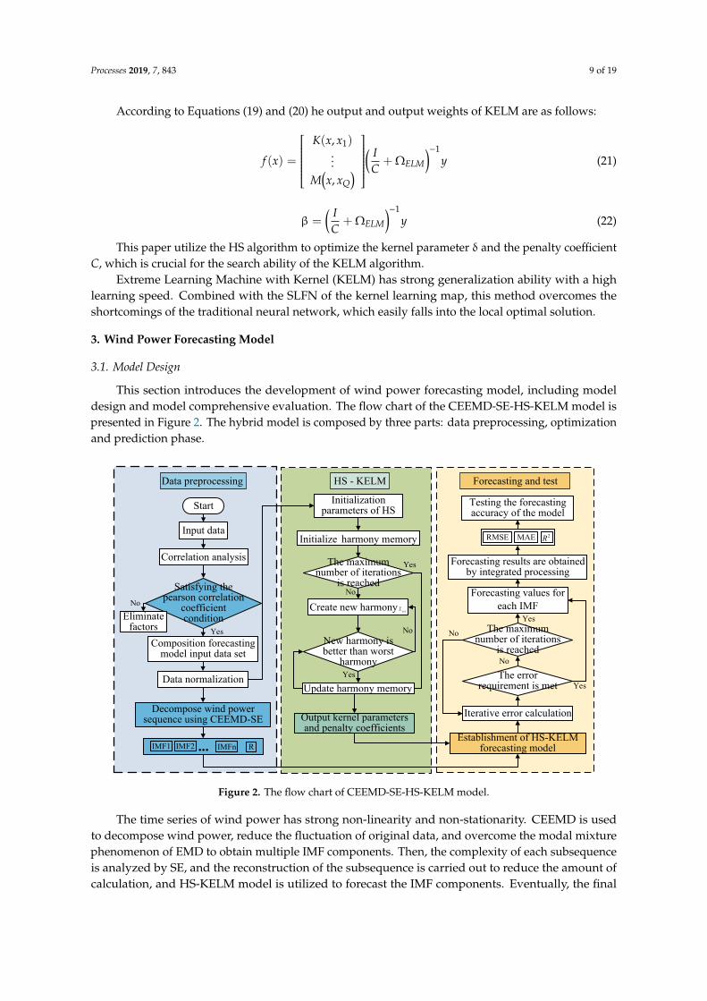
This section introduces the development of wind power forecasting model, including modeldesign and model comprehensive evaluation. The flow chart of the CEEMD-SE-HS-KELM model ispresented in Figure 2. The hybrid model is composed by three parts: data preprocessing, optimizationand prediction phase.

Processes 2019, 7, x FOR PEER REVIEW 9 of 19

( ) 2, exp 2i j i jK x x x x= − − δ (20)

According to Equations (19) and (20) he output and output weights of KELM are as follows:

( )( )

( )11,

,ELM

Q

K x x If x yCM x x

− = + Ω

M (21)

1

= ELMI yC

− β + Ω

(22)

This paper utilize the HS algorithm to optimize the kernel parameter δ and the penalty coefficient C, which is crucial for the search ability of the KELM algorithm.

Extreme Learning Machine with Kernel (KELM) has strong generalization ability with a high learning speed. Combined with the SLFN of the kernel learning map, this method overcomes the shortcomings of the traditional neural network, which easily falls into the local optimal solution.

3. Wind Power Forecasting Model

3.1. Model Design

This section introduces the development of wind power forecasting model, including model design and model comprehensive evaluation. The flow chart of the CEEMD-SE-HS-KELM model is presented in Figure 2. The hybrid model is composed by three parts: data preprocessing, optimization and prediction phase.

Start Initialization parameters of HS

Correlation analysis

Input data

Decompose wind power sequence using CEEMD-SE

Data normalization

Satisfying the pearson correlation

coefficient condition

No

Eliminate factors Yes

Initialize harmony memory

Output kernel parameters and penalty coefficients

The maximum number of iterations

is reachedNo

Create new harmony

New harmony is better than worst

harmony

Update harmony memory

Yes

Yes

No

newX

Establishment of HS-KELM forecasting model

Forecasting values for each IMF

Testing the forecasting accuracy of the model

Data preprocessing HS - KELM Forecasting and test

Composition forecasting model input data set

...IMF1 IMF2 IMFn R

Forecasting results are obtained by integrated processing

RMSE MAE 2R

The maximum number of iterations

is reached

Iterative error calculation

The error requirement is met Yes

Yes

No

No

Figure 2. The flow chart of CEEMD-SE-HS-KELM model.

The time series of wind power has strong non-linearity and non-stationarity. CEEMD is used to decompose wind power, reduce the fluctuation of original data, and overcome the modal mixture phenomenon of EMD to obtain multiple IMF components. Then, the complexity of each subsequence is analyzed by SE, and the reconstruction of the subsequence is carried out to reduce the amount of calculation, and HS-KELM model is utilized to forecast the IMF components. Eventually, the final

Figure 2. The flow chart of CEEMD-SE-HS-KELM model.

The time series of wind power has strong non-linearity and non-stationarity. CEEMD is usedto decompose wind power, reduce the fluctuation of original data, and overcome the modal mixturephenomenon of EMD to obtain multiple IMF components. Then, the complexity of each subsequenceis analyzed by SE, and the reconstruction of the subsequence is carried out to reduce the amount ofcalculation, and HS-KELM model is utilized to forecast the IMF components. Eventually, the final

Processes 2019, 7, 843 10 of 19

wind power forecasting results are obtained through integrated processing. This paper establishes aCEEMD-SE-HS-KELM model to forecast wind power, as shown below:

(1) Screen the original data set through correlation analysis to obtain data indicators with highcorrelation, which can used as the input data of CEEMD-HS-KELM forecasting model;

(2) Decompose the original wind power sequence X through CEEMD method to obtain n subsequences components from high frequency to low frequency, which are n − 1 intrinsic modefunction IMFi(t) and one approximately monotonous residual R(t);

(3) Utilize SE theory to calculate the complexity of each subsequence and reconstruct the subsequencedecomposed by CEEMD;

(4) HS-KELM model is constructed for each subsequence and the forecast values of each subsequenceare obtained;

(5) Superimpose the wind power forecasting results of each subsequence to obtain the finalforecasting results.

3.2. Evaluation Criteria

For the performance test of the proposed model, three evaluation criteria are of great importance,including Root Mean Square Error (RMSE), Mean Absolute Error (MAE) and Determination Factor R2.The calculation methods are as follows:

RMSE =

√√1n

n∑i=1

(pi − p′i

)2(23)

MAE =1n

N∑i=1

∣∣∣p′i − pi∣∣∣ (24)

R2 =

n∑i=1

(p′i − pi

)2

n∑i=1

(pi − pi)2 (25)

where: pi represents the true power value, kW; p′i represents the anti-normalized power value afterCEEMD-SE-HS-KELM output, kW; n represents the data number.

4. Short-Term Wind Power Forecasting

To comprehensively verify the performance of the CEEMD-SE-HS-KELM wind power hybridforecasting model proposed in this paper, the following case is designed. Taking the measured data ofa wind farm in China as an example, short-term wind power is made by the hybrid forecasting model,and compared with many intelligent forecasting models, multiple error indicators are calculated, andthe fitting effect and forecasting accuracy of the model are analyzed.

The wind power data of Beijing wind farm in May 2017 is selected as experimental sample. Therated installed capacity of the wind farm is 49 MW and the sampling frequency is one point per 5 min.The data of 17 consecutive days from May 15th to 31st are taken, totaling 4608 sampling points, ofwhich the first 4322 sampling points are training sets of the forecasting model. The last 288 samplingpoints are the test set, the original data is in the “Supplementary Materials”.

4.1. Data Set Screening

The original data sets are divided into two categories, one is historical meteorological data,including historical wind power data and historical weather data such as wind speed and wind

Processes 2019, 7, 843 11 of 19

direction. According to the Pearson correlation coefficients analysis of the original data sets, theobserved correlations degrees between the meteorological data and wind power are shown in Table 1.

Table 1. Pearson correlation coefficient analysis results.

Indicators Correlation Indicators Correlation Indicators Correlation

windspeed

10 m 0.788

winddirection

10 m −0.391 temperature 0.22730 m 0.796 30 m −0.308 humidity −0.5150 m 0.777 50 m −0.025 rainfall 0.2970 m 0.764 70 m 0.289 pressure −0.37

hub height 0.764 hub height 0.289 -

According to the Pearson correlation coefficients, the coupling degree between wind speed, winddirection and wind power are relatively high, so the wind speeds of different heights, the wind directionof 30 m, the wind direction of 50 m are selected as the input variables of the model. The original data isconverted into a number between [0, 1], the purpose of which is to eliminate the magnitude differencebetween the various dimensions of data and avoid the influence on the forecasting result caused by thelarge magnitude difference between input and output data. The normalization method is as follows:

x∗i =xi − xmin

xmax − xmin(26)

where: xmin and xmax are respectively the minimum and the maximum value in the sequence, xi is theinitial input data, and x∗i is the normalized data.

4.2. CEEMD Decomposition of Wind Power Sequence and Subsequence Reconstruction

The original wind power data is decomposed by CEEMD decomposition method, and 12 IMFcomponents and 1 residual component are obtained. The result of decomposition is shown in Figure 3.After CEEMD decomposition processing, the characteristic changes of the signal are extracted fromhigh frequency to low frequency, and the components are relatively stable.


Table 1. Pearson correlation coefficient analysis results.

Indicators Correlation Indicators Correlation Indicators Correlation

wind speed

10 m 0.788

wind direction

10 m −0.391 temperature 0.227 30 m 0.796 30 m −0.308 humidity −0.51 50 m 0.777 50 m −0.025 rainfall 0.29 70 m 0.764 70 m 0.289 pressure −0.37 hub

height 0.764 hub

height 0.289 -

According to the Pearson correlation coefficients, the coupling degree between wind speed, wind direction and wind power are relatively high, so the wind speeds of different heights, the wind direction of 30 m, the wind direction of 50 m are selected as the input variables of the model. The original data is converted into a number between [0, 1], the purpose of which is to eliminate the magnitude difference between the various dimensions of data and avoid the influence on the forecasting result caused by the large magnitude difference between input and output data. The normalization method is as follows:

min

max min

ii

x xxx x

∗ −=−

(26)

where: m inx and maxx are respectively the minimum and the maximum value in the sequence, ix is the initial input data, and ix

∗ is the normalized data.

4.2. CEEMD Decomposition of Wind Power Sequence and Subsequence Reconstruction

The original wind power data is decomposed by CEEMD decomposition method, and 12 IMF components and 1 residual component are obtained. The result of decomposition is shown in Figure 3. After CEEMD decomposition processing, the characteristic changes of the signal are extracted from high frequency to low frequency, and the components are relatively stable.

Figure 3. Decomposition results of CEEMD.

Using the HS-KELM model to directly forecast each subsequence will increase the amount of computation. SE method is used to calculate the complexity of each subsequence, and the results are shown in Figure 4.

0 500 1000 1500 2000 2500 3000 3500 40000

150

Orig

inal

0 500 1000 1500 2000 2500 3000 3500 4000-10

0

10

IMF

2

0 500 1000 1500 2000 2500 3000 3500 4000-2

0

2

IMF

3

0 500 1000 1500 2000 2500 3000 3500 4000-5

0

5

IMF

4

0 500 1000 1500 2000 2500 3000 3500 4000-20

0

20

IMF

5

0 500 1000 1500 2000 2500 3000 3500 4000-50

0

50

IMF

6

0 500 1000 1500 2000 2500 3000 3500 4000-50

0

50

IMF

7

0 500 1000 1500 2000 2500 3000 3500 4000-50

0

50

IMF

8

0 500 1000 1500 2000 2500 3000 3500 4000-100

0

100

IMF

9

0 500 1000 1500 2000 2500 3000 3500 4000-50

0

50

IMF

10

0 500 1000 1500 2000 2500 3000 3500 4000-50

0

50

IMF

11

0 500 1000 1500 2000 2500 3000 3500 4000-10

0

10

IMF

12

0 500 1000 1500 2000 2500 3000 3500 4000-10

0

10

IMF

13

0 500 1000 1500 2000 2500 3000 3500 400030

40

50

R

Figure 3. Decomposition results of CEEMD.

Using the HS-KELM model to directly forecast each subsequence will increase the amount ofcomputation. SE method is used to calculate the complexity of each subsequence, and the results areshown in Figure 4.

Processes 2019, 7, 843 12 of 19Processes 2019, 7, x FOR PEER REVIEW 12 of 19

Figure 4. Sample entropy of each subsequence.

The criterion of SE for IMF sequence classification is about 0.2 times of the original sequence standard deviation [49]. By calculating the standard deviation of subsequence complexity, the standard deviation is 0.25, so the similarity difference of subsequence reconstruction is obtained. The value is 0.12 and is rounded down to 0.1. As shown in Figure 5, the sample entropy of IMF2 and IMF3 subsequences has small difference, and the two subsequences can be classified into one class, and integrated and reconstructed as a new subsequence input into the HS-KELM for training and forecasting. All subsequences are categorized and the results are presented in Table 2 and the reconstructed results are presented in Figure 5.

Table 2. Results of the new subsequence with merged intrinsic mode functions (IMF) components.

New Subsequence Number

Initial Subsequence Number



1 1 5 7 2 2,3 6 8,9 3 4 7 10,11,12 4 5,6 8 R

Figure 5. Wind power sub-sequences processed by CEEMD-SE.

IMF1 IMF2 IMF3 IMF4 IMF5 IMF6 IMF7 IMF8 IMF9 IMF10 IMF11 IMF12 R0

0.2

0.4

0.6

0.8

1

1.2

1.4

1.6

1.8

The sequence number

Sam

ple

entro

py

1.166

1.73 1.719

0.706

0.422

0.33

0.202

0.0760.057

0.019 0.008 0.006 0.0004

0 500 1000 1500 2000 2500 3000 3500 4000 4500

-5

0

5

IMF

1

0 500 1000 1500 2000 2500 3000 3500 4000 4500

-5

0

5

IMF

2

0 500 1000 1500 2000 2500 3000 3500 4000 4500

-10-505

10

IMF

3

0 500 1000 1500 2000 2500 3000 3500 4000 4500-40

-20

0

20

40

IMF

4

0 500 1000 1500 2000 2500 3000 3500 4000 4500-20-10

01020

IMF

5

0 500 1000 1500 2000 2500 3000 3500 4000 4500

-50

0

50

IMF

6

0 500 1000 1500 2000 2500 3000 3500 4000 4500-50

0

50

IMF

7

0 500 1000 1500 2000 2500 3000 3500 4000 4500

35

40

45

R

Time point/(5min)Time point/(5min)


The criterion of SE for IMF sequence classification is about 0.2 times of the original sequencestandard deviation [49]. By calculating the standard deviation of subsequence complexity, the standarddeviation is 0.25, so the similarity difference of subsequence reconstruction is obtained. The valueis 0.12 and is rounded down to 0.1. As shown in Figure 5, the sample entropy of IMF2 and IMF3subsequences has small difference, and the two subsequences can be classified into one class, andintegrated and reconstructed as a new subsequence input into the HS-KELM for training and forecasting.All subsequences are categorized and the results are presented in Table 2 and the reconstructed resultsare presented in Figure 5.



The criterion of SE for IMF sequence classification is about 0.2 times of the original sequence standard deviation [49]. By calculating the standard deviation of subsequence complexity, the standard deviation is 0.25, so the similarity difference of subsequence reconstruction is obtained. The value is 0.12 and is rounded down to 0.1. As shown in Figure 5, the sample entropy of IMF2 and IMF3 subsequences has small difference, and the two subsequences can be classified into one class, and integrated and reconstructed as a new subsequence input into the HS-KELM for training and forecasting. All subsequences are categorized and the results are presented in Table 2 and the reconstructed results are presented in Figure 5.






1 1 5 7 2 2,3 6 8,9 3 4 7 10,11,12 4 5,6 8 R


IMF1 IMF2 IMF3 IMF4 IMF5 IMF6 IMF7 IMF8 IMF9 IMF10 IMF11 IMF12 R0

0.2

0.4

0.6

0.8

1

1.2

1.4

1.6

1.8

The sequence number

Sam

ple

entro

py

1.166

1.73 1.719

0.706

0.422

0.33

0.202

0.0760.057

0.019 0.008 0.006 0.0004

0 500 1000 1500 2000 2500 3000 3500 4000 4500

-5

0

5

IMF

1

0 500 1000 1500 2000 2500 3000 3500 4000 4500

-5

0

5

IMF

2

0 500 1000 1500 2000 2500 3000 3500 4000 4500

-10-505

10

IMF

3

0 500 1000 1500 2000 2500 3000 3500 4000 4500-40

-20

0

20

40

IMF

4

0 500 1000 1500 2000 2500 3000 3500 4000 4500-20-10

01020

IMF

5

0 500 1000 1500 2000 2500 3000 3500 4000 4500

-50

0

50

IMF

6

0 500 1000 1500 2000 2500 3000 3500 4000 4500-50

0

50

IMF

7

0 500 1000 1500 2000 2500 3000 3500 4000 4500

35

40

45

R

Time point/(5min)Time point/(5min)



New SubsequenceNumber

Initial SubsequenceNumber

New SubsequenceNumber

Initial SubsequenceNumber

1 1 5 72 2,3 6 8,93 4 7 10,11,124 5,6 8 R

Processes 2019, 7, 843 13 of 19

4.3. Wind Power Forecasting by CEEMD-SE-HS-KELM Model

Following decomposition and reconstruction for the sequences, 8 HS-KELM forecasting modelsare constructed, and the above 8 subsequences are respectively trained and forecast. For the HS-KELMmodel, the common values of 3 parameters HMCR, PAR and BW of HS algorithm is [0.63, 0.99],[0.01, 0.73] and [0.0004, 0.3] respectively [41,50], the maximum iteration limit is detailed in reference [51],and the objective function is set as RMSE. Therefore, HMS = 100, HMCR = 0.9, PAR = 0.35, BW = 0.25,the number of new harmony vectors generated each time is 10.

For the HS-KELM model, the number of hidden layer neurons is set to 20, the data of a certainday is randomly selected and the wind power is forecast. RMSE is selected as the objective function,and the number of terminations is set as 100. As shown in Figure 6, the target function value tendsto be gentle after 21 iterations, and ends at the 100th generation. The convergence speed is faster,and it is more consistent with the actual power curve. Therefore, the forecasting model structure ofHS-KELM model is set as “6-20-1”. Train and forecast the eight subsequences respectively, and thefinal forecasting results of each subsequence are integrated to get the wind power forecasting outputvalue, as shown in Figure 7.



Following decomposition and reconstruction for the sequences, 8 HS-KELM forecasting models are constructed, and the above 8 subsequences are respectively trained and forecast. For the HS-KELM model, the common values of 3 parameters HMCR , PAR and BW of HS algorithm is [0.63,0.99] , [0.01,0.73] and [0.0004,0.3] respectively [41,50], the maximum iteration limit is detailed in reference [51], and the objective function is set as RMSE. Therefore, 100HMS = ,

0.9HMCR= , 0.35PAR= , 0.25BW = , the number of new harmony vectors generated each time is 10.

For the HS-KELM model, the number of hidden layer neurons is set to 20, the data of a certain day is randomly selected and the wind power is forecast. RMSE is selected as the objective function, and the number of terminations is set as 100. As shown in Figure 6, the target function value tends to be gentle after 21 iterations, and ends at the 100th generation. The convergence speed is faster, and it is more consistent with the actual power curve. Therefore, the forecasting model structure of HS-KELM model is set as “6-20-1”. Train and forecast the eight subsequences respectively, and the final forecasting results of each subsequence are integrated to get the wind power forecasting output value, as shown in Figure 7.

Figure 6. Iteration curve.

0 10 20 30 40 50 60 70 80 90 1000

20

40

60

80

100

120

Iteration times

Obj

ectiv

e fu

nctio

n va

lue/

RM

SE

The number of termination iterations is 100

0 50 100 150 200 250 300

-5

0

5

IMF

1

0 50 100 150 200 250 300

-5

0

5

IMF

2

0 50 100 150 200 250 300-10

0

10

IMF

3

0 50 100 150 200 250 300-20

0

20

IMF

4

0 50 100 150 200 250 300

-10

0

10

IMF

5

0 50 100 150 200 250 300-50

0

50

IMF

6

0 50 100 150 200 250 3000

10

20

IMF

7

0 50 100 150 200 250 30035.1

35.2

35.3

IMF

8

0 50 100 150 200 250 3000

50

100

Fore

casti

ng re

sults

Actual Value Forecasting Value

Time point /(5min)




Following decomposition and reconstruction for the sequences, 8 HS-KELM forecasting models are constructed, and the above 8 subsequences are respectively trained and forecast. For the HS-KELM model, the common values of 3 parameters HMCR , PAR and BW of HS algorithm is [0.63,0.99] , [0.01,0.73] and [0.0004,0.3] respectively [41,50], the maximum iteration limit is detailed in reference [51], and the objective function is set as RMSE. Therefore, 100HMS = ,

0.9HMCR= , 0.35PAR= , 0.25BW = , the number of new harmony vectors generated each time is 10.

For the HS-KELM model, the number of hidden layer neurons is set to 20, the data of a certain day is randomly selected and the wind power is forecast. RMSE is selected as the objective function, and the number of terminations is set as 100. As shown in Figure 6, the target function value tends to be gentle after 21 iterations, and ends at the 100th generation. The convergence speed is faster, and it is more consistent with the actual power curve. Therefore, the forecasting model structure of HS-KELM model is set as “6-20-1”. Train and forecast the eight subsequences respectively, and the final forecasting results of each subsequence are integrated to get the wind power forecasting output value, as shown in Figure 7.


0 10 20 30 40 50 60 70 80 90 1000

20

40

60

80

100

120

Iteration times

Obj

ectiv

e fu

nctio

n va

lue/

RM

SE

The number of termination iterations is 100

0 50 100 150 200 250 300

-5

0

5

IMF

1

0 50 100 150 200 250 300

-5

0

5

IMF

2

0 50 100 150 200 250 300-10

0

10

IMF

3

0 50 100 150 200 250 300-20

0

20

IMF

4

0 50 100 150 200 250 300

-10

0

10

IMF

5

0 50 100 150 200 250 300-50

0

50

IMF

6

0 50 100 150 200 250 3000

10

20

IMF

7

0 50 100 150 200 250 30035.1

35.2

35.3

IMF

8

0 50 100 150 200 250 3000

50

100

Fore

casti

ng re

sults

Actual Value Forecasting Value

Time point /(5min)

Figure 7. Wind power forecasting results.

Processes 2019, 7, 843 14 of 19

4.4. Comparative Analysis of Forecasting Models

To confirm the validity of this model, ELM, KELM, HS-KELM, EMD-SE-HS-KELM,CEEMD-SE-HS-KELM models are constructed for comparative analysis, and they are respectivelynamed configuration #1–#5. The KELM structure is in the form of “6-20-1”, and the maximum numberof training time is 500. To avoid the influence of randomness on the forecasting results, the averagevalue of each model is taken after 50 independent runs and compared with the actual wind power.The forecasting results are presented in Figure 8.


Figure 7. Wind power forecasting results.

4.4. Comparative Analysis of Forecasting Models

To confirm the validity of this model, ELM, KELM, HS-KELM, EMD-SE-HS-KELM, CEEMD-SE-HS-KELM models are constructed for comparative analysis, and they are respectively named configuration #1–#5. The KELM structure is in the form of “6-20-1”, and the maximum number of training time is 500. To avoid the influence of randomness on the forecasting results, the average value of each model is taken after 50 independent runs and compared with the actual wind power. The forecasting results are presented in Figure 8.

To compare and evaluate forecasting accuracy of different models, determination coefficient R2 and model error indexes such as Root Mean Square Error (RMSE) and Mean Absolute Error (MAE) are calculated respectively, as shown in Table 3 and Figure 9.

Table 3. The calculation results of model evaluation index.

Evaluation Index ELM KELM HS-KELM

EMD-SE-HS-KELM

CEEMD-SE-HS-KELM

Configuration #1 #2 #3 #4 #5 RMSE 20.84 15.63 9.74 4.67 2.16 MAE 9.29 7.05 3.86 0.52 0.39

R2 1.12 1.05 0.96 1.03 1.01

Figure 8. Wind power forecasting results (5 min). (a) configuration #1: ELM model; (b) configuration #2: KELM model; (c) configuration #3: HS-KELM model; (d) configuration #4: EMD-SE-HS-KELM model; (e) configuration #5: CEEMD-SE-HS-KELM model; (f) comparison of forecasting values of different models.

0 50 100 150 200 250

0

20

40

60

80

100

Win

d po

wer

/MW

0 50 100 150 200 250

-6

-4

-2

0

2

4

6

Time/5min

Erro

r/MW

Configuration #5

ActualConfiguration #5

(e)

0 50 100 150 200 250-20

0

20

40

60

80

100

120

Win

d po

wer

/MW


0 50 100 150 200 250

-40

-20

0

20

Time/5min

Erro

r/MW

Configuration #2

(b)0 50 100 150 200 250

0

20

40

60

80

100

120

Win

d po

wer

/MW


0 50 100 150 200 250-60

-40

-20

0

20

40

60

Time/5min

Erro

r/MW

Configuration #1

(a)

0 50 100 150 200 250

0

20

40

60

80

100

120W

ind

pow

er/M

W

Actual DataConfiguration #4

0 50 100 150 200 250-15

-10

-5

0

5

10

15

Time/5min

Erro

r/MW

Configuration #4

(d)0 50 100 150 200 250

0

20

40

60

80

100

Win

d po

wer

/MW


0 50 100 150 200 250-30

-20

-10

0

10

20

30

Time/5min

Erro

r/MW

Configuration #3

(c)

0 50 100 150 200 250-20

0

20

40

60

80

100

120

Win

d Po

wer

/MW

Time/5min

Actual Configuration #5Configuration #4Configuration #3Configuration #2Configuration #1

(f)

Figure 8. Wind power forecasting results (5 min). (a) configuration #1: ELM model; (b) configuration#2: KELM model; (c) configuration #3: HS-KELM model; (d) configuration #4: EMD-SE-HS-KELMmodel; (e) configuration #5: CEEMD-SE-HS-KELM model; (f) comparison of forecasting values ofdifferent models.

To compare and evaluate forecasting accuracy of different models, determination coefficient R2

and model error indexes such as Root Mean Square Error (RMSE) and Mean Absolute Error (MAE) arecalculated respectively, as shown in Table 3 and Figure 9.

Table 3. The calculation results of model evaluation index.

EvaluationIndex ELM KELM HS-KELM EMD-SE-HS-KELM CEEMD-SE-HS-KELM

Configuration #1 #2 #3 #4 #5

RMSE 20.84 15.63 9.74 4.67 2.16MAE 9.29 7.05 3.86 0.52 0.39

R2 1.12 1.05 0.96 1.03 1.01

Processes 2019, 7, 843 15 of 19Processes 2019, 7, x FOR PEER REVIEW 15 of 19

Figure 9. Root Mean Square Error (RMSE) and Mean Absolute Error (MAE) and R2 of different forecasting models.

It can be seen from Table 3 and Figure 8, Figure 9:

(1) Comparing EMD-SE-HS-KELM and CEEMD-SE-HS-KELM, the RMSE and MAE of the latter are improved by 53.63% and 24.36% respectively compared with EMD-SE-HS-KELM, which indicates that the hybrid model of data preprocessing based on CEEMD-HS has better processing effect.

(2) Comparing HS-KELM and EMD-SE-HS-KELM, the RMSE and MAE of the latter are improved by 52.10% and 86.58%, respectively, compared with HS-KELM, which indicates that for non-stationary wind power series, pre-processing can effectively eliminate noise, ensure data quality and improve forecasting accuracy.

(3) Comparing KELM and HS-KELM, the RMSE and MAE of the latter are improved by 37.67% and 45.23%, respectively, compared with KELM, which indicates that the parameters of KELM algorithm are optimized by HS algorithm, which effectively improves the search ability and the forecasting accuracy.

(4) Compared with ELM, the RMSE and MAE of the KELM are improved by 25.02% and 24.06% respectively compared with ELM, which indicates that the forecasting accuracy of KELM algorithm is better than ELM model, and KELM has a stronger generalization ability.

It can be seen from Figure 8, that a single KELM and ELM forecasting model can only roughly reflect the wind power trend, but the forecasting value at each time point is quite different from the actual. The CEEMD-SE-HS-KELM hybrid forecasting model constructed in this paper has a good fitting effect between the forecasting result and the actual value at each time point, and its forecasting accuracy is higher.

5. Conclusions

Aiming at short-term forecasting of non-linear and unsteady wind power time series, a hybrid forecasting model consisting of CEEMD-SE and HS optimized KELM is proposed in this paper. Firstly, the Pearson correlation coefficient is used to screen the input data to reduce data redundancy. Secondly, the combined data preprocessing strategy of CEEMD-SE is utilized to process the data. The wind power time series is decomposed and reconstructed to eliminate data noise and reduce the computational load. After that, the KELM model optimized by HS is used to forecast each subsequence after reconstructing, and the final wind power forecasting value is obtained after integration processing. Finally, a specific wind farm in China is taken as an example, the CEEMD-SE-HS-KELM, EMD-SE-HS-KELM, HS-KELM, KELM and ELM models are established to forecast wind power respectively. The case study shows that:

(1) KELM model has higher forecasting accuracy than ELM model, and has broad application prospects in wind power forecasting.

#1#2

#3 #4

#5

0

5

10

15

20

25

RMSE

#1#2

#3 #4

#5

0

2

4

6

8

10

MAE

#1#2

#3 #4

#5

0

0.5

1

1.5

R-Square

Configuration #1 Configuration #2 Configuration #3 Configuration #4 Configuration #5

Figure 9. Root Mean Square Error (RMSE) and Mean Absolute Error (MAE) and R2 of differentforecasting models.

It can be seen from Table 3 and Figure 8, Figure 9:

(1) Comparing EMD-SE-HS-KELM and CEEMD-SE-HS-KELM, the RMSE and MAE of the latter areimproved by 53.63% and 24.36% respectively compared with EMD-SE-HS-KELM, which indicatesthat the hybrid model of data preprocessing based on CEEMD-HS has better processing effect.

(2) Comparing HS-KELM and EMD-SE-HS-KELM, the RMSE and MAE of the latter are improved by52.10% and 86.58%, respectively, compared with HS-KELM, which indicates that for non-stationarywind power series, pre-processing can effectively eliminate noise, ensure data quality and improveforecasting accuracy.

(3) Comparing KELM and HS-KELM, the RMSE and MAE of the latter are improved by 37.67%and 45.23%, respectively, compared with KELM, which indicates that the parameters of KELMalgorithm are optimized by HS algorithm, which effectively improves the search ability and theforecasting accuracy.

(4) Compared with ELM, the RMSE and MAE of the KELM are improved by 25.02% and 24.06%respectively compared with ELM, which indicates that the forecasting accuracy of KELM algorithmis better than ELM model, and KELM has a stronger generalization ability.

It can be seen from Figure 8, that a single KELM and ELM forecasting model can only roughlyreflect the wind power trend, but the forecasting value at each time point is quite different from theactual. The CEEMD-SE-HS-KELM hybrid forecasting model constructed in this paper has a goodfitting effect between the forecasting result and the actual value at each time point, and its forecastingaccuracy is higher.

5. Conclusions

Aiming at short-term forecasting of non-linear and unsteady wind power time series, a hybridforecasting model consisting of CEEMD-SE and HS optimized KELM is proposed in this paper. Firstly,the Pearson correlation coefficient is used to screen the input data to reduce data redundancy. Secondly,the combined data preprocessing strategy of CEEMD-SE is utilized to process the data. The wind powertime series is decomposed and reconstructed to eliminate data noise and reduce the computational load.After that, the KELM model optimized by HS is used to forecast each subsequence after reconstructing,and the final wind power forecasting value is obtained after integration processing. Finally, a specificwind farm in China is taken as an example, the CEEMD-SE-HS-KELM, EMD-SE-HS-KELM, HS-KELM,KELM and ELM models are established to forecast wind power respectively. The case study shows that:

(1) KELM model has higher forecasting accuracy than ELM model, and has broad applicationprospects in wind power forecasting.

Processes 2019, 7, 843 16 of 19

(2) Compared with the single KELM model, HS can optimize the kernel parameters and penaltyfunction of KELM to obtain higher forecasting accuracy, which indicates that HS-KELM modelhas stronger global search ability and more stable forecasting performance.

(3) Compared with EMD-SE, the data preprocessing strategy based on CEMD-SE has betterperformance and effectively improves the forecasting accuracy. The hybrid model proposed inthis paper can be well applied to short-term wind power forecasting.

Supplementary Materials: The following are available online at http://www.mdpi.com/2227-9717/7/11/843/s1.

Author Contributions: All of the authors have contributed to this research. K.W., L.S. and H.Z. collected the dataand wrote this paper; D.N. provided professional guidance; J.L. collected the data, G.D. and X.X. revised thismanuscript. All authors have approved the submitted manuscript.

Funding: This work was supported by the 2018 Key Projects of Philosophy and Social Sciences Research, Ministryof Education, China (grant number 18JZD032); 111 Project, (grant number B18021); Natural Science Foundation ofChina (grant number 71804045).

Conflicts of Interest: The authors declare no conflict of interest.

Nomenclature

NWP Numerical weather predictionANN Artificial neural networkSVM Support vector machineLSSVM Least squares support vector machinePCA Principal component analysisWT Wavelet transformEMD Empirical mode decompositionEWT Empirical wavelet transformCEEMD Complementary ensemble empirical mode decompositionWAS Wavelet neural networkDWT Discrete wavelet transformGARCH Generalized autoregressive conditional heteroscedasticMkRVR Multi-kernel relevance vector regressionIMF Intrinsic mode functionsMLFFNN Multilayer feed-forward neural networkSVR Support vector regressionRBF Radial basis functionANFIS Adaptive neuro-fuzzy inference systemPSO Particle swarm optimizationVMD Variational mode decompositionBA Bat algorithmELM Extreme learning machineCSO Crisscross optimization algorithmKELM Extreme learning machine with kernelHS Harmony searchSE Sample entropyHM Harmony memoryHMS Harmony memory sizeHMCR Harmony memory considering ratePCR Pitch adjusting rateBW BandwidthBPNN Back propagation neural networkRMSE Root mean square errorMAE Mean absolute errorR2 Determining factor

Processes 2019, 7, 843 17 of 19

References

1. Cai, W.; Lai, K.-H.; Liu, C.; Wei, F.; Ma, M.; Jia, S.; Jiang, Z.; Lv, L. Promoting sustainability of manufacturingindustry through the lean energy-saving and emission-reduction strategy. Sci. Total Environ. 2019, 665, 23–32.[CrossRef] [PubMed]

2. Cai, W.; Liu, C.; Lai, K.-H.; Li, L.; Cunha, J.; Hu, L. Energy performance certification in mechanicalmanufacturing industry: A review and analysis. Energy Convers. Manag. 2019, 186, 415–432. [CrossRef]

3. Hong, C.; Lin, W.M.; Wen, B.Q. Review of wind speed and wind power prediction methods for wind farms.Power Syst. Clean Energy. 2011, 27, 60–66.

4. Ren, Y.; Suganthan, P.N.; Srikanth, N. A novel empirical mode decomposition with support vector regressionfor wind speed forecasting. IEEE Trans. Neural Netw. Learn. Syst. 2016, 27, 1793–1798. [CrossRef] [PubMed]

5. Zhao, X.; Wang, C.; Su, J.; Wang, J. Research and application based on the swarm intelligence algorithm andartificial intelligence for wind farm decision system. Renew. Energy 2019, 134, 681–697. [CrossRef]

6. National Energy Administration. China Power Industry Annual Development Report: Renewable EnergyAdded Capacity Accounts for Over 50%. Available online: http://www.nea.gov.cn/2019-06/19/c_138155207.htm (accessed on 19 June 2019).

7. Zhang, C.; Zhou, J.; Li, C.; Fu, W.; Peng, T. A compound structure of ELM based on feature selection andparameter optimization using hybrid backtracking search algorithm for wind speed forecasting. EnergyConvers. Manag. 2017, 143, 360–376. [CrossRef]

8. Tasnim, S.; Rahman, A.; Oo, A.M.T.; Haque, M.E. Wind power prediction in new stations based on knowledgeof existing stations: A cluster based multi source domain adaptation approach. Knowl. Based Syst. 2018, 145,15–24. [CrossRef]

9. Wang, J.; Du, P.; Niu, T.; Yang, W. A novel hybrid system based on a new proposed algorithm-Multi-ObjectiveWhale Optimization Algorithm for wind speed forecasting. Appl. Energy 2017, 208, 344–360. [CrossRef]

10. Li, H.; Wang, J.; Lu, H.; Guo, Z. Research and application of a combined model based on variable weight forshort term wind speed forecasting. Renew. Energy 2018, 116, 669–684. [CrossRef]

11. Feng, S.L.; Wang, W.S.; Liu, C.; Dai, H.Z. Study on the physical approach to wind power prediction.Proc. CSEE 2010, 30, 1–6.

12. Yang, W.; Wang, J.; Lu, H.; Niu, T.; Du, P. Hybrid wind energy forecasting and analysis system based ondivide and conquer scheme: A case study in China. J. Clean. Prod. 2019, 222, 942–959. [CrossRef]

13. Zhang, W.; Qu, Z.; Zhang, K.; Mao, W.; Ma, Y.; Fan, X. A combined model based on CEEMDAN andmodified flower pollination algorithm for wind speed forecasting. Energy Convers. Manag. 2017, 136, 439–451.[CrossRef]

14. Jiang, P.; Yang, H.; Heng, J. A hybrid forecasting system based on fuzzy time series and multi-objectiveoptimization for wind speed forecasting. Appl. Energy 2019, 235, 786–801. [CrossRef]

15. Hao, Y.; Tian, C. The study and application of a novel hybrid system for air quality early-warning. Appl. SoftComput. 2019, 74, 729–746. [CrossRef]

16. Wang, Y.; Wang, J.; Wei, X. A hybrid wind speed forecasting model based on phase space reconstructiontheory and Markov model: A case study of wind farms in northwest China. Energy 2015, 91, 556–572.[CrossRef]

17. Sun, W.; Liu, M. Wind speed forecasting using FEEMD echo state networks with RELM in Hebei, China.Energy Convers. Manag. 2016, 114, 197–208. [CrossRef]

18. Lahouar, A.; Slama, J.B.H. Hour-ahead wind power forecast based on random forests. Renew. Energy 2017,109, 529–541. [CrossRef]

19. Li, C.; Zhu, Z. Research and application of a novel hybrid air quality early-warning system: A case study inChina. Sci. Total Environ. 2018, 626, 1421–1438. [CrossRef] [PubMed]

20. Xiao, L.; Shao, W.; Yu, M.; Ma, J.; Jin, C. Research and application of a hybrid wavelet neural network modelwith the improved cuckoo search algorithm for electrical power system forecasting. Appl. Energy 2017, 198,203–222. [CrossRef]

21. Li, G.; Shi, J.; Zhou, J. Bayesian adaptive combination of short-term wind speed forecasts from neural networkmodels. Renew. Energy 2011, 36, 352–359. [CrossRef]

22. Liu, D.; Niu, D.; Wang, H.; Fan, L. Short-term wind speed forecasting using wavelet transform and supportvector machines optimized by genetic algorithm. Renew. Energy 2014, 62, 592–597. [CrossRef]

Processes 2019, 7, 843 18 of 19

23. Hu, J.; Wang, J.; Ma, K. A hybrid technique for short-term wind speed prediction. Energy 2015, 81, 563–574.[CrossRef]

24. Zhou, J.; Shi, J.; Li, G. Fine tuning support vector machines for short-term wind speed forecasting. EnergyConvers. Manag. 2011, 52, 1990–1998. [CrossRef]

25. Li, H.; Wang, J.; Li, R.; Lu, H. Novel analysis-forecast system based on multi-objective optimization for airquality index. J. Clean. Prod. 2019, 208, 1365–1383. [CrossRef]

26. Huang, G.-B.; Zhou, H.; Ding, X.; Zhang, R. Extreme learning machine for regression and multiclassclassification. IEEE Trans. Syst. Man Cybern. Part B Cybern. 2011, 42, 513–529. [CrossRef] [PubMed]

27. Zhang, Y.; Zhang, C.; Zhao, Y.; Gao, S. Wind speed prediction with RBF neural network based on PCA andICA. J. Electr. Eng. 2018, 69, 148–155. [CrossRef]

28. Huang, Y.; Shen, L.; Liu, H. Grey relational analysis, principal component analysis and forecasting of carbonemissions based on long short-term memory in China. J. Clean. Prod. 2019, 209, 415–423. [CrossRef]

29. Qi, J.; Xu, C.Z.; Liu, Y.Q.; Han, S.; Li, L. Short-term wind power prediction method based on wind speedcloud model in similar day. Autom. Electr. Power Syst. 2018, 42, 53–59.

30. Gilles, J. Empirical wavelet transform. IEEE Trans. Signal Process. 2013, 61, 3999–4010. [CrossRef]31. Naik, J.; Satapathy, P.; Dash, P. Short-term wind speed and wind power prediction using hybrid empirical

mode decomposition and kernel ridge regression. Appl. Soft Comput. 2018, 70, 1167–1188. [CrossRef]32. Du, P.; Wang, J.Z.; Yang, W.D.; Niu, T. A novel hybrid model for short-term wind power forecasting. Appl. Soft

Comput. 2019, 80, 93–106. [CrossRef]33. Jiang, P.; Wang, Y.; Wang, J. Short-term wind speed forecasting using a hybrid model. Energy 2017, 119,

561–577. [CrossRef]34. Jiang, Y.; Huang, G.; Peng, X.; Li, Y.; Yang, Q. A novel wind speed prediction method: Hybrid of

correlation-aided DWT, LSSVM and GARCH. J. Wind Eng. Ind. Aerodyn. 2018, 174, 28–38. [CrossRef]35. Fei, S.W. A hybrid model of EMD and multiple-kernel RVR algorithm for wind speed prediction. Int. J.

Electr. Power Energy Syst. 2016, 78, 910–915. [CrossRef]36. Khosravi, A.; Koury, R.; Machado, L.; Pabon, J. Prediction of wind speed and wind direction using artificial

neural network, support vector regression and adaptive neuro-fuzzy inference system. Sustain. EnergyTechnol. Assess. 2018, 25, 146–160. [CrossRef]

37. Wu, Q.; Lin, H.X. Short-term wind speed forecasting based on hybrid variational mode decompositionand least squares support vector machine optimized by bat algorithm model. Sustainability 2019, 11, 652.[CrossRef]

38. Jiang, Y.; Huang, G.; Yang, Q.; Yan, Z.; Zhang, C. A novel probabilistic wind speed prediction approach usingreal time refined. Energy Convers. Manag. 2019, 185, 758–773. [CrossRef]

39. Tian, C.; Hao, Y.; Hu, J. A novel wind speed forecasting system based on hybrid data preprocessing andmulti-objective optimization. Appl. Energy 2018, 231, 301–319. [CrossRef]

40. Yin, H.; Dong, Z.; Chen, Y.; Ge, J.; Lai, L.L.; Vaccaro, A.; Meng, A. An effective secondary decompositionapproach for wind power forecasting using extreme learning machine trained by crisscross optimization.Energy Convers. Manag. 2017, 150, 108–121. [CrossRef]

41. Geem, Z.W.; Kim, J.H.; Loganathan, G.V. A new heuristic optimization algorithm: Harmony search. Simulation2001, 76, 60–68. [CrossRef]

42. Richman, J.S.; Moorman, J.R. Physiological time-series analysis using approximate entropy and sampleentropy. Am. J. Physiol. Heart Circ. Physiol. 2000, 278, H2039–H2049. [CrossRef] [PubMed]

43. Huang, N.E.; Shen, Z.; Long, S.R.; Wu, M.C.; Shih, H.H.; Zheng, Q.; Yen, N.-C.; Tung, C.C.; Liu, H.H.The empirical mode decomposition and the Hilbert spectrum for nonlinear and non-stationary time seriesanalysis. Proc. R. Soc. A: Math. Phys. Eng. Sci. 1998, 454, 903–995. [CrossRef]

44. Yeh, J.R.; Shieh, J.S.; Huang, N.E. Complementary ensemble empirical mode decomposition: A novel noiseenhanced data analysis method. Adv. Adapt. Data Anal. 2010, 2, 135–156. [CrossRef]

45. Lin, T.; Cai, R.Q.; Zhang, L.; Yang, X.; Liu, G.; Liao, W.J. Prediction intervals forecasts of wind power basedon IBA-KELM. Renew. Energy Resour. 2018, 7, 23.

46. Bapat, K.M.P.B. The Generalized Moore-Penrose Inverses. Linear Algebra Appl. 1992, 165, 59–69.47. Huang, G.-B. An insight into extreme learning machines: Random neurons, random features and kernels.

Cogn. Comput. 2014, 6, 376–390. [CrossRef]

Processes 2019, 7, 843 19 of 19

48. Li, D. Kernel Function. In Encyclopedia of Microfluidics and Nanofluidics; Springer: Boston, MA, USA, 2008.[CrossRef]

49. Hornero, R. Optimal parameters study for sample entropy-based atrial fibrillation organization analysis.Comput. Methods Programs Biomed. 2010, 99, 124–132.

50. Kim, J.H.; Geem, Z.W.; Kim, E.S. Parameter estimation of the nonlinear muskingum model using harmonysearch. J. Am. Water Resour. Assoc. 2001, 37, 1131–1138. [CrossRef]

51. Omran Mahamed, G.H.; Mahdavi, M. Global-best harmony search. Appl. Math. Comput. 2008, 198, 643–656.

© 2019 by the authors. Licensee MDPI, Basel, Switzerland. This article is an open accessarticle distributed under the terms and conditions of the Creative Commons Attribution(CC BY) license (http://creativecommons.org/licenses/by/4.0/).

Powered by TCPDF (www.tcpdf.org)

http://www.tcpdf.org

wind power short-term forecasting hybrid model based on...

Documents