wind stress parameterisation in the southern ocean · wind stress parameterisation in the southern...

Wind Stress Parameterisation in the Southern

Ocean

A thesis submitted in partial fulfilment of the requirements forthe degree of Bachelor of Philosophy (Science) with Honours

by

David Karel Hutchinson

Supervisor:Dr. Andrew McC. Hogg

Geophysical Fluid Dynamics GroupResearch School of Earth SciencesThe Australian National University

5 November 2008

Declaration

This thesis is an account of research undertaken between February 2008 and November2008 at The Research School of Earth Sciences, The Australian National University,Canberra, Australia.

Except where acknowledged in the customary manner, the material presented inthis thesis is, to the best of my knowledge, original and has not been submitted inwhole or part for a degree in any university.

David K. Hutchinson5 November 2008

iii

Acknowledgements

Firstly I would like to thank my supervisor Andy Hogg, for his astute direction andencouragement throughout the year. He has almost always made himself available toanswer my questions, and his feedback on earlier drafts of this thesis was invaluable.Thanks also to all of the GFD group for making me feel very welcome here, and for allthe interesting discussions over lunch and coffee. It has been a privilege to spend myhonours year here.

I would like to thank mum, dad and Henry for supporting me throughout the year,and for making life easy for me living at home. I must also thank them for helpingme get through the earlier years of my degree, especially in the times when I lackedenthusiasm (i.e. most of second year!), as it was their support that got me throughthose years. Dad also gave me useful feedback on my thesis too, which was muchappreciated. Thanks also to Tamsin for her support, for all the fun times we hadthroughout the year, and for being so flexible around my study and rowing needs.Thanks to the boys club: Dan, Lee, and Robin, for all the fun times involving pool,cards, board games, Wii sports, and beer. I’d also like to mention the guys from theANU boat club for keeping me doing regular exercise, and for the great time we hadat uni games.

I would also like to acknowledge the support of an A.L. Hales Scholarship providedby RSES. This work was supported by the National Facility of the Australian Partner-ship for Advanced Computing.

v

Abstract

Wind stress is often parameterised in ocean-atmosphere coupled models by a simpledrag law, which depends quadratically on the atmospheric velocity at a reference height.Strictly speaking, this drag law should be written as a quadratic function of the differ-ence between the ocean and atmosphere velocities. The two different cases give verysimilar magnitudes of stress, however recent studies have shown that including theocean velocity in the calculation of stress leads to a significant reduction in wind powerinput to the ocean. While this effect has previously been modelled in gyre circulations,this work is the first to investigate it in the Southern Ocean, using the eddy-resolvingquasi-geostrophic coupled model Q-GCM. In this model, including the ocean velocityin the stress calculation is found to reduce power input, but paradoxically the circum-polar transport is increased. The increase in transport is a consequence of two mainfactors: eddy saturation of the Antarctic Circumpolar Current, and eddy damping un-der the ocean velocity dependent stress. This result is unique to the Southern Ocean,and it adds to the substantial body of evidence that the Southern Ocean can only bemodelled accurately if eddies are resolved.

The wind stress parameterisation scheme is also modified to include temperaturecoupling in the Southern Ocean. Scatterometer observations have established a stronglink between wind stress gradients and sea surface temperature (SST) gradients, dueto convection in the atmospheric boundary layer caused by SST fronts. A simplemodification to the wind stress is implemented, coupling the quadratic drag law to thetemperature difference between the ocean and atmosphere. This simple representationis shown to be consistent with scatterometer observations, and the coupling constantis calibrated using known correlations between stress and SST in the Southern Ocean.Unlike the ocean velocity dependent stress, the temperature coupled stress is found tohave a negligible effect on the mean flow in this model.

vii

Contents

Declaration iii

Acknowledgements v

Abstract vii

1 Introduction 11.1 Components of the Ocean Circulation . . . . . . . . . . . . . . . . . . . 1

1.1.1 Geostrophic Circulation . . . . . . . . . . . . . . . . . . . . . . . 21.1.2 Ocean Gyres . . . . . . . . . . . . . . . . . . . . . . . . . . . . . 31.1.3 Dynamics of the ACC . . . . . . . . . . . . . . . . . . . . . . . . 41.1.4 Meridional Overturning Circulation . . . . . . . . . . . . . . . . 7

1.2 Wind Stress Dependence on Ocean Velocity . . . . . . . . . . . . . . . . 71.2.1 Power Input to the Oceans . . . . . . . . . . . . . . . . . . . . . 81.2.2 Estimate of Power Difference . . . . . . . . . . . . . . . . . . . . 9

1.3 Wind Stress Dependence on SST . . . . . . . . . . . . . . . . . . . . . . 101.3.1 Correlations between SST and Wind Stress . . . . . . . . . . . . 111.3.2 Modelling the Atmospheric Response . . . . . . . . . . . . . . . . 111.3.3 Modelling the Ocean Response . . . . . . . . . . . . . . . . . . . 12

1.4 Project Aims . . . . . . . . . . . . . . . . . . . . . . . . . . . . . . . . . 13

2 Model: Q-GCM 152.1 Dynamic Features . . . . . . . . . . . . . . . . . . . . . . . . . . . . . . 15

2.1.1 Quasi-Geostrophic Equations . . . . . . . . . . . . . . . . . . . . 152.1.2 Mixed Layers . . . . . . . . . . . . . . . . . . . . . . . . . . . . . 182.1.3 Fixed Atmosphere Pressure . . . . . . . . . . . . . . . . . . . . . 19

2.2 Wind Stress . . . . . . . . . . . . . . . . . . . . . . . . . . . . . . . . . . 212.2.1 Stress as a Function of Atmosphere Velocity . . . . . . . . . . . . 222.2.2 Ocean Velocity Dependent Stress . . . . . . . . . . . . . . . . . 242.2.3 Temperature Coupled Stress . . . . . . . . . . . . . . . . . . . . 26

2.3 Program Modifications . . . . . . . . . . . . . . . . . . . . . . . . . . . . 262.3.1 Wind Power Input . . . . . . . . . . . . . . . . . . . . . . . . . . 262.3.2 Temperature Coupling . . . . . . . . . . . . . . . . . . . . . . . . 27

3 Ocean Velocity Dependent Stress 293.1 Wind Stress Differences . . . . . . . . . . . . . . . . . . . . . . . . . . . 293.2 Power Input . . . . . . . . . . . . . . . . . . . . . . . . . . . . . . . . . . 30

3.2.1 Spatial Distribution . . . . . . . . . . . . . . . . . . . . . . . . . 30

ix

x Contents

3.2.2 Spatially Averaged Power . . . . . . . . . . . . . . . . . . . . . . 313.3 Circumpolar Transport . . . . . . . . . . . . . . . . . . . . . . . . . . . . 33

3.3.1 Eddy Saturation . . . . . . . . . . . . . . . . . . . . . . . . . . . 333.3.2 Eddy Damping Effect . . . . . . . . . . . . . . . . . . . . . . . . 36

3.4 Transient Kinetic Energy . . . . . . . . . . . . . . . . . . . . . . . . . . 373.5 Discussion . . . . . . . . . . . . . . . . . . . . . . . . . . . . . . . . . . . 39

4 Temperature Coupled Stress 434.1 Calibration of Coupling Constant . . . . . . . . . . . . . . . . . . . . . . 43

4.1.1 Sea-Air Temperature Difference . . . . . . . . . . . . . . . . . . . 434.1.2 Directional Correlations Between Stress and SST . . . . . . . . . 454.1.3 Test Values of κ . . . . . . . . . . . . . . . . . . . . . . . . . . . 454.1.4 Other Factors Affecting Calibration . . . . . . . . . . . . . . . . 50

4.2 Flow Results . . . . . . . . . . . . . . . . . . . . . . . . . . . . . . . . . 514.2.1 Ekman Velocity . . . . . . . . . . . . . . . . . . . . . . . . . . . . 514.2.2 Power Input . . . . . . . . . . . . . . . . . . . . . . . . . . . . . . 524.2.3 Circumpolar Transport . . . . . . . . . . . . . . . . . . . . . . . 534.2.4 Kinetic Energy . . . . . . . . . . . . . . . . . . . . . . . . . . . . 54

4.3 Discussion . . . . . . . . . . . . . . . . . . . . . . . . . . . . . . . . . . . 56

5 Conclusion 595.1 Ocean Velocity Dependent Stress . . . . . . . . . . . . . . . . . . . . . . 595.2 Temperature Coupled Stress . . . . . . . . . . . . . . . . . . . . . . . . . 595.3 Future Directions . . . . . . . . . . . . . . . . . . . . . . . . . . . . . . . 60

Bibliography 63

List of Figures

1.1 A simplistic Stommel model reproduced from Vallis (2006) showing (a)wind stress varying sinusoidally in the y direction; (b) streamfunctionof the resulting gyre circulation. There is a strong northward flow alongthe western boundary, and a much slower southward return flow in theinterior. . . . . . . . . . . . . . . . . . . . . . . . . . . . . . . . . . . . . 4

1.2 Illustration of the different processes by which momentum is trans-ferred downwards in an ACC-like channel (reproduced from Hallbergand Gnanadesikan, 2001). In each scheme, wind stress at the surface isbalanced by bottom (ie: topographic) form stress, and the northwardEkman flux from the wind is balanced by a southward geostrophic flux.Eastward momentum is transferred downwards via diapycnal overturn-ing in scheme (a), and by interfacial form stress created by eddies inschemes (b) and (c). . . . . . . . . . . . . . . . . . . . . . . . . . . . . . 6

1.3 A schematic of the wind velocity u, as a function of height z, in theatmospheric boundary layer. H is the reference height, at which au ismeasured. Fig. (a) shows the velocity profile in thermal equilibrium(based on Vallis, 2006, Fig. 2.10), while (b) shows a velocity profile thathas been perturbed by convective upwelling. . . . . . . . . . . . . . . . . 10

2.1 Schematic diagram of the layered structure of Q-GCM (not to scale).The QG dynamics of the atmosphere are prescribed by a fixed pressurefield; only the ocean and the mixed layers are allowed to evolve in time. 16

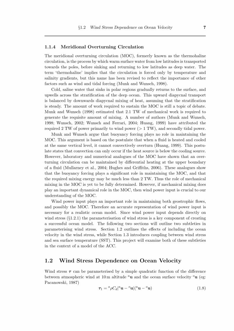
2.2 Comparison of the zonal mean wind stress from the NCEP, SOC and HRclimatologies, with that of the present model. Only the domain of thepresent model is shown here, with the centre of the domain: y = 1440km, corresponding to 55S. The southern edge of the domain: y = 0 km,corresponds to 68S. . . . . . . . . . . . . . . . . . . . . . . . . . . . . . 22

2.3 (a) Zonally averaged atmospheric velocity (black) plotted with its corres-ponding pressure (red); (b) zonally averaged ocean dynamic wind stresscomponents. . . . . . . . . . . . . . . . . . . . . . . . . . . . . . . . . . . 23

3.1 Comparison of zonal wind stress between (a) oτx0 from S0, and (b) oτx

1

from simulation S1. Since oτx0 depends only on the atmospheric velocity,

it varies only in the y direction. A similar pattern is seen in oτx1 , with

additional variations due to the ocean velocity. . . . . . . . . . . . . . . 30

xi

xii LIST OF FIGURES

3.2 (a) |ou1|, (b) P1 and (c) Pdiff as calculated from simulation S1, witheach quantity time averaged over 50 years. Both P1 and Pdiff are largein magnitude above regions of high velocity. . . . . . . . . . . . . . . . . 31

3.3 Time series of the area averaged power input. Both P1 and P0 arecalculated in simulation S1, whereas only P0 is calculated in simulationS0. The above curves were smoothed using a low-pass Fourier filter,with a cutoff frequency of 0.5 years−1. This filtering method applies toall of the subsequent time series presented in this thesis. . . . . . . . . . 32

3.4 Layer 1 mean streamfunctions of (a) S0 and (b) S1; instantaneous layer1 streamfunctions of (c) S0 and (d) S1, taken at t = 120 years in eachcase; (e) topography anomaly. The direction of the flow is similar inboth simulations, and is closely linked to the topography. Jets appearto meander around elevated topography, and are stronger above valleys. 34

3.5 (a) Total transport, and (b) layer 1 transport, for simulation S0 (blue),and the extended run (red) with a 25% reduction in wind stress. Thesystem is forced using the τ0 parameterisation in both cases. . . . . . . 35

3.6 (a) Total transport, and (b) layer 1 transport, for simulation S1 (blue),and the extended run (red) with a 25% reduction in wind stress. Thesystem is forced using the τ1 parameterisation in both cases. The ap-parent discontinuity between the blue and red trends is caused by thelow pass filters applied to each trend separately. Without filtering, theblue and red trends would join up (although there would be much morehigh frequency noise). . . . . . . . . . . . . . . . . . . . . . . . . . . . . 36

3.7 Schematic diagram of the eddy damping effect of using τ1, reproducedfrom Zhai and Greatbatch (2007). (a) A constant wind blowing over acircularly symmetric eddy. Under τ0 forcing, the wind stress magnitudeis the same at the top and the bottom of the eddy. Under τ1 forcing, themagnitude of stress is weakened on the upper half, and strengthened onthe lower half, which damps the eddy in both cases. (b) The contributionof the ocean velocity to the wind stress, which damps the flow of the eddy. 37

3.8 Time series of Layer 1 kinetic energy for each simulations. . . . . . . . . 38

4.1 A snapshot at 15 years of (a) SST, (b) atmospheric surface temperature(AST), and (c) their difference ∆T . It is clear from a visual comparisonthat regions of large |∆T | correlate strongly with SST gradients in thex direction. . . . . . . . . . . . . . . . . . . . . . . . . . . . . . . . . . . 44

4.2 (a) Correlations between the perturbation crosswind SST gradient (∇T × τ )′ · kand the curl of the perturbation wind stress (∇ × τ ′) · k, with (b) ahistogram of observations. (c) Correlations between the perturbationdownwind SST gradient (∇T · τ )′ and the divergence of the perturba-tion wind stress ∇·τ ′, with (d) a histogram of observations. In each bin,the ‘x’ marker represents the mean, and the error bar is ±1 standarddeviation. Based on a 3 year simulation with κ = 0.1 C−1. . . . . . . . 46

LIST OF FIGURES xiii

4.3 (a) and (b): Same as Fig. 4.2a and 4.2c respectively, but with a restricteddomain and a least squares linear fit. αc and αd are the slopes of therespective linear models. The above data were calculated from a 3 yearsimulation using κ = 0.1 C−1. . . . . . . . . . . . . . . . . . . . . . . . . 47

4.4 αc and αd plotted as a function of κ, where each point is generated froma 3 year simulation. Each trend shows a least squares linear fit, used tocalibrate κ to 0.23 C−1. . . . . . . . . . . . . . . . . . . . . . . . . . . . 48

4.5 Directional Coupling results for the calibrated model, using κ = 0.23 C−1,with the same domain restrictions as in Figs. 4.3a,b. The results areaggregated from a 30 year simulation. . . . . . . . . . . . . . . . . . . . 48

4.6 Zonal wind stress oτx plotted as a function of y, comparing the defaultstress DS with the three-quarter stress TS and half stress HS schemes. . 50

4.7 Comparison of time averaged Ekman velocity of (a) S0 and (b) Sκ; with(c) the contribution of ∆T . . . . . . . . . . . . . . . . . . . . . . . . . . 52

4.8 (a) Layer 1 velocity |ou1|; (b) time averaged power 〈Pκ〉 from Sκ; (c)the difference in power 〈Pκ〉 − 〈P0〉, between the Sκ and S0 simulations.Unlike Pdiff, the power difference 〈Pκ〉 − 〈P0〉 does not correlate verystrongly with velocity. . . . . . . . . . . . . . . . . . . . . . . . . . . . . 53

4.9 Time series of power input from the S0 simulation (red) and the Sκ

simulation, marked P0 and Pκ respectively. The Pκ series is translatedon the time axis to begin at the same point in time as P0. . . . . . . . . 54

4.10 Time averaged streamfunctions for (a) S0, and (b) Sκ, showing a verysimilar pattern of flow for both. . . . . . . . . . . . . . . . . . . . . . . . 55

4.11 Time series of (a) total transport, and (b) layer 1 transport. In eachplot, the blue trend is from the Sκ simulation, and the red trend is fromthe S0 simulation. . . . . . . . . . . . . . . . . . . . . . . . . . . . . . . 55

4.12 Time series of layer 1 KE for simulations S0 (red) and Sκ (blue). . . . . 564.13 Reproduced from Fig. 2 of Hogg et al. (2008), showing the pattern

of circulation in their model. (a) mean SST (Contour Interval 2C);(b) mean upper layer streamfunction (CI 2 Sv). The dashed lines arenegative contours, and the bold line is the zero contour. . . . . . . . . . 57

xiv LIST OF FIGURES

List of Tables

2.1 Description of the symbols used in the Q-GCM equations. . . . . . . . . 172.2 Fixed parameter values for simulations, divided into global, ocean and

atmosphere components. . . . . . . . . . . . . . . . . . . . . . . . . . . . 202.3 Parameters which are adjusted for the two different experiments, separ-

ated into ocean and atmosphere parameters. ‘Value 1’ corresponds tothe ocean velocity difference simulations, while ‘Value 2’ corresponds tothe windstress-sst coupling simulations. . . . . . . . . . . . . . . . . . . 21

2.4 Summary of wind stress schemes. . . . . . . . . . . . . . . . . . . . . . . 23

3.1 Comparison of circumpolar transport between simulations S0 and S1. . 333.2 Layer 1 quantities of mean flow KE, TKE and total KE for each simu-

lation. Simulation S0 has a greater KE, from both mean and transientcontributions. . . . . . . . . . . . . . . . . . . . . . . . . . . . . . . . . . 39

4.1 Comparison of our calibrated model, with observational data in the SOfrom O’Neill et al. (2003) and Chelton et al. (2004). We chose to tune ourmodel to O’Neill et al. (2003), since we are following their methodologyfor calculating the αc and αd coefficients. . . . . . . . . . . . . . . . . . 49

4.2 Comparison between the Default Stress (DS), Three-Quarter Stress (TS)and Half Stress (HS) schemes of the αc and αd coefficients, and the re-scaled coefficients φc and φd. . . . . . . . . . . . . . . . . . . . . . . . . 51

4.3 Comparison of transport between the Sκ and S0 simulations. . . . . . . 544.4 Layer 1 quantities of mean flow KE, TKE and total KE for Sκ and S0. . 54

xv

xvi LIST OF TABLES

Chapter 1

Introduction

This thesis is based upon a model of the circulation in the Southern Ocean (SO). Inparticular, the model deals with the Antarctic Circumpolar Current (ACC), a regionwhere the ocean circulation is unblocked by continental boundaries. The focus is ontwo problems in parameterising wind stress. Wind stress is parameterised by a draglaw, which depends quadratically on the difference between the atmosphere and oceanvelocities (Eq. 1.8). This drag law can also be approximated using the atmosphere ve-locity only (Eq. 1.9). This thesis compares the circumpolar flow under these two stressregimes, and how they affect the wind power input to the ocean. The second problemis the impact of sea surface temperature fronts (SST) in altering local stress patterns.These SST interactions with the wind stress are modelled by a simple modification tothe quadratic drag law (Eq. 1.21). This chapter begins by outlining some features ofocean circulation that motivate the investigation of wind stress. This is followed by areview of recent studies on the two areas of interest. The chapter concludes by settingout the aims of this project.

1.1 Components of the Ocean Circulation

The oceans are of primary importance to the Earth’s climate, in terms of regulatingtemperature and heat transport. For example, the entire atmosphere has the sameheat capacity as only the top three metres of the oceans. This great difference in heatcapacity means that heat transfer at an ocean-atmosphere interface largely acts toregulate the temperature of the atmosphere to that of the ocean. Another consequenceof the ocean’s large heat capacity is that most of the heat energy absorbed from solarradiation is stored in the oceans. Ocean circulation plays a key role in redistributingthis heat.

The Earth is approximately in thermal equilibrium, with the incoming solar radi-ation balanced by the outgoing blackbody radiation. The incoming radiation is highlydependent on latitude, with much higher intensity at low latitudes (near the equator)than at high latitudes (near the poles). If we ignore the Earth’s axial tilt, the dailyaverage solar radiation I at a given latitude θ is given by (eg: Vallis, 2006)

I(θ) =S

π(1− α) cos θ (1.1)

1

2 Introduction

where S is the solar constant, and α is the earth’s albedo. This representation ofI captures the basic latitudinal dependence of solar radiation, without including thedetails of seasonal changes (due to the axial tilt).

The emitted blackbody radiation E given by Stefan’s Law, depends only on tem-perature T (in Kelvin):

E = σT 4 (1.2)

where σ is the Stefan-Boltzmann constant. Earth’s temperature range is mostly con-fined within a few tens of degrees of its average temperature (288 K), so the outgoingradiation is much more uniform than the incoming radiation. This gives rise to netheating in equatorial regions, and net cooling in high latitudes. It is partly via theoceans that this excess heat is transported from the equator towards the poles.

Circulation in the oceans can be divided into two distinct types. The first typeis near-horizontal, geostrophic circulation, forced primarily by the wind. Two typesof geostrophic circulation are discussed below; ocean gyres, which are found in themajority of the world’s ocean basins, and the zonally re-entrant channel flow of theACC. The second type of ocean circulation is the meridional overturning circulation(MOC), which communicates water between the surface and the abyssal ocean. Bothtypes of circulation are important to the transport of heat from equator to poles.

1.1.1 Geostrophic Circulation

The primitive momentum equation for a fluid in the rotating reference frame of theEarth is (eg: Pedlosky, 1987)

DuDt

+ 2Ω× u = −∇pρ

+ g +F

ρ(1.3)

where u is velocity, t is time, D/Dt = ∂/∂t+u · ∇ is the advective derivative, Ω is theEarth’s angular velocity, p is the pressure, ρ is the density, g = −gk is the gravitationalvector and F represents the dissipation due to friction. The coordinate system is chosento align with geopotential surfaces, where x and y are the coordinates in the eastwardand northward directions respectively, and z is in the ‘vertical’ direction, pointing outof the Earth’s surface. In the remainder of this section the effects of friction are ignored,setting F ≈ 0. Since vertical motions are typically small compared to horizontal ones,the z component of the momentum equation reduces to the hydrostatic balance

∂p

∂z= −ρg. (1.4)

The horizontal components of the momentum equation can be simplified when scaled bythe characteristic velocity U , the characteristic lengthscale L and the Coriolis parameterf = 2Ω sin θ. The Rossby number Ro = U/fL is the ratio of inertial accelerations toCoriolis accelerations, which summarises the importance of the Earth’s rotation to theflow. If Ro 1, then the advective terms in Eq. (1.3) can be ignored, leaving abalance between the Coriolis acceleration and the pressure gradient. This is known as

§1.1 Components of the Ocean Circulation 3

the geostrophic approximation (eg: Pedlosky, 1987), and is given in cartesian form as

fu = −1ρ

∂p

∂y(1.5a)

fv =1ρ

∂p

∂x(1.5b)

where u and v are the velocity components in the eastward and northward directionsrespectively. The geostrophic approximation gives a steady state description of thelarge scale flows in the ocean and atmosphere, and does not allow for time-dependentvelocity fields. Although it is a greatly simplified model, it gives an accurate descriptionof most ocean surface currents.

1.1.2 Ocean Gyres

Since the geostrophic equations are steady-state only, they must be coupled to anequation of state, such as an advective buoyancy equation, to allow for time-dependentflows. The resulting problem is non-linear and cannot be solved analytically. TheStommel model (Stommel, 1948) simplifies this by vertically integrating over the oceandepth. This eliminates the thermodynamics, giving a model which is linear and dependsonly on the wind stress (Vallis, 2006). The Stommel model assumes a flat-bottomedocean, with friction parameterised by linear drag at the ocean floor. It relates themeridional velocity v (the overbar indicates a depth integrated quantity), to the windstress curl:

βv = curlz(τt − τb) (1.6)

where β = ∂f/∂y is assumed to be constant, τt is the wind stress at the ocean surface,and τb is the stress at the ocean floor. curlz( ) is defined as the z-component ofthe vector curl operator ∇ × ( ). The Munk model (Munk, 1950) makes the samesimplifications, but instead uses drag at the sidewalls, rather than the ocean floor. TheStommel-Munk model uses friction both at the sidewalls, and at the ocean floor.

If bottom friction is small, it is possible to simplify Equation (1.6) to a balancebetween wind stress and meridional velocity:

βv ≈ curlzτt. (1.7)

This is known as Sverdrup balance (Sverdrup, 1947). It gives a useful qualitative de-scription of meridional geostrophic flow in an ocean gyre system. Figure 1.1 shows anillustration of Sverdrup balance, applied to a rectangular box ocean basin. The sinus-oidal wind stress forces a gyre circulation as shown in the streamfunction. The windstress curl is negative, which causes a negative meridional velocity (southward) throughthe interior of the basin. The strong western boundary current is a consequence of thevariation of the Coriolis parameter with latitude (Stommel, 1948). Although Sverdrupbalance gives a useful description of gyre circulation, its quantitative predictions arenot always consistent with observations. This is mainly due to non-negligible verticalvelocities, which are explicitly ignored in the derivation of Eq. (1.6).

4 Introduction

Figure 1.1: A simplistic Stommel model reproduced from Vallis (2006) showing (a) wind stressvarying sinusoidally in the y direction; (b) streamfunction of the resulting gyre circulation.There is a strong northward flow along the western boundary, and a much slower southwardreturn flow in the interior.

Sverdrup balance requires a pressure difference between the east and west bound-aries of the ocean basin. Across the latitude band of Drake Passage in the SO, theSverdrup balance does not apply (Rintoul et al., 2001), because there are no zonalboundaries to support a pressure difference. A pressure profile around a zonal contourmust return to its original value, which implies that there is no net meridional geo-strophic flow: v = 0. The ACC is dynamically unique, since it is the only major oceancurrent with no zonal boundaries.

1.1.3 Dynamics of the ACC

Since Sverdrup balance does not apply in the ACC, the flow must be limited by otherfactors. The flow of the ACC is balanced primarily by momentum gained at thesurface (from the westerly wind) and lost at the ocean floor. This is in contrast to gyreflows, which are controlled by the wind stress curl (Eq. 1.7). Thermodynamic effectsmay also be important, however the momentum balance is thought to be the primarymechanism limiting the flow. Friction plays only a minor role in the momentum balanceof the ACC. If the flow is assumed to be limited by friction either at the sides or thebottom of the current, then the computed transport is at least an order of magnitudegreater than the observed value (of order 100 Sv), using accepted values of lateraland vertical viscosity (Munk and Palmen, 1951). Early attempts to model the ACCcould not explain the observed transport using realistic constraints of both wind stressand friction (eg: Hidaka and Tsuchiya, 1953; Gill, 1968). This has become known as

§1.1 Components of the Ocean Circulation 5

Hidaka’s dilemma.

In light of the discrepancy between friction based models and observations, Munkand Palmen (1951) proposed that the ACC transport is not limited by friction, but bytopographic form stress, also known as mountain drag. This is a process by which flowacross topographic features creates pressure gradients, which oppose the flow. Since theactual measurement of topographic form stress is not feasible, models have providedthe only method of testing Munk and Palmen’s hypothesis.

A major hurdle for numerical models of the ACC is that the momentum balancedepends greatly on the resolution of the model. Coarse resolution models of the ACC,where the grid length is larger than the eddy radius, do not support Munk and Palmen’shypothesis (Gill and Bryan, 1971; Bryan and Cox, 1972). This is because the verticalviscosity is too small to create a downward momentum flux sufficient to balance theinput of momentum from the wind stress. On the other hand, models which resolveeddies do support the concept of topographic form stress balancing the wind stressfrom the surface (McWilliams et al., 1978; Wolff et al., 1991).

Eddies create interfacial form stress, which acts to transfer momentum downwardsmuch faster than viscous shear forces. Straub (1993) argued that in the presence ofeddies, the transport of the ACC may actually be independent of wind stress (providedthat the stress is at least large enough to create baroclinic instability in the first place).Using a two-layer quasi-geostrophic (QG) model of the ACC, Straub argued that thevelocity of the flow is approximately limited to the velocity at which baroclinic instabil-ity first develops. This theory, also known as eddy saturation, can give a reasonableestimate of the transport of the ACC. However, the eddy saturation theory assumesthat baroclinic instability is dominant throughout the channel, whereas it may only beconfined to regions of elevated topography (Hallberg and Gnanadesikan, 2001). An-other issue is that under eddy saturation, the predicted transport is highly dependenton the stratification (Straub, 1993; Hallberg and Gnanadesikan, 2001; Hogg and Blun-dell, 2006).

Diapycnal overturning may also be important in setting the transport of the ACC.It has been argued that the eastward momentum gained at the surface is commu-nicated down to bottom water through buoyancy-driven overturning, where a west-ward topographic form stress can then limit the flow (Gent et al., 2001; Hallbergand Gnanadesikan, 2001). Figure 1.2 (reproduced from Hallberg and Gnanadesikan,2001) illustrates the different processes by which momentum is transferred downwards,showing (a) diapycnal fluxes, (b) stationary eddies, and (c) transient eddies. Diapycnaloverturning also plays a key role in setting the stratification, which directly affects thetransport under eddy saturated flow. Therefore QG models of the ACC are limited,since they explicitly ignore thermodynamic effects, and cannot simulate overturning.

In this project we use a three layer QG model of the ACC, with a fixed stratifica-tion. We work under the hypothesis that the downward transfer of momentum is, tofirst order, created by eddy-related interfacial form stress, and overturning effects areignored.

6 Introduction

Figure 1.2: Illustration of the different processes by which momentum is transferred down-wards in an ACC-like channel (reproduced from Hallberg and Gnanadesikan, 2001). In eachscheme, wind stress at the surface is balanced by bottom (ie: topographic) form stress, and thenorthward Ekman flux from the wind is balanced by a southward geostrophic flux. Eastwardmomentum is transferred downwards via diapycnal overturning in scheme (a), and by interfacialform stress created by eddies in schemes (b) and (c).

§1.2 Wind Stress Dependence on Ocean Velocity 7

1.1.4 Meridional Overturning Circulation

The meridional overturning circulation (MOC), formerly known as the thermohalinecirculation, is the process by which warm surface water from low latitudes is transportedtowards the poles, before sinking and returning to low latitudes as deep water. Theterm ‘thermohaline’ implies that the circulation is forced only by temperature andsalinity gradients, but this name has been revised to reflect the importance of otherfactors such as wind and tidal forcing (Munk and Wunsch, 1998).

Cold, saline water that sinks in polar regions gradually returns to the surface, andupwells across the stratification of the deep ocean. This upward diapycnal transportis balanced by downwards diapycnal mixing of heat, assuming that the stratificationis steady. The amount of work required to sustain the MOC is still a topic of debate.Munk and Wunsch (1998) estimated that 2.1 TW of mechanical work is required togenerate the requisite amount of mixing. A number of authors (Munk and Wunsch,1998; Wunsch, 2002; Wunsch and Ferrari, 2004; Huang, 1999) have attributed therequired 2 TW of power primarily to wind power (> 1 TW), and secondly tidal power.

Munk and Wunsch argue that buoyancy forcing plays no role in maintaining theMOC. This argument is based on the postulate that when a fluid is heated and cooledat the same vertical level, it cannot convectively overturn (Huang, 1999). This postu-late states that convection can only occur if the heat source is below the cooling source.However, laboratory and numerical analogues of the MOC have shown that an over-turning circulation can be maintained by differential heating at the upper boundaryof a fluid (Mullarney et al., 2004; Hughes and Griffiths, 2006). These analogues showthat the buoyancy forcing plays a significant role in maintaining the MOC, and thatthe required mixing energy may be much less than 2 TW. Thus the role of mechanicalmixing in the MOC is yet to be fully determined. However, if mechanical mixing doesplay an important dynamical role in the MOC, then wind power input is crucial to ourunderstanding of the MOC.

Wind power input plays an important role in maintaining both geostrophic flows,and possibly the MOC. Therefore an accurate representation of wind power input isnecessary for a realistic ocean model. Since wind power input depends directly onwind stress (§1.2.1) the parameterisation of wind stress is a key component of creatinga successful ocean model. The following two sections will outline two subtleties inparameterising wind stress. Section 1.2 outlines the effects of including the oceanvelocity in the wind stress, while Section 1.3 introduces coupling between wind stressand sea surface temperature (SST). This project will examine both of these subtletiesin the context of a model of the ACC.

1.2 Wind Stress Dependence on Ocean Velocity

Wind stress τ can be parameterised by a simple quadratic function of the differencebetween atmospheric wind at 10 m altitude au and the ocean surface velocity ou (eg:Pacanowski, 1987)

τ1 = aρCd|au− ou|(au− ou) (1.8)

8 Introduction

where aρ is the density of air at sea level and Cd is the drag coefficient, which is ap-proximated as a constant. Standard wind stress parameterisations often neglect the oucontribution, because typical atmospheric velocities are of order au ∼ 10 ms−1, whilstocean velocities on a basin scale are ou ∼ 0.1 ms−1. Thus Eq (1.8) is approximatedby setting au − ou ≈ au, giving a wind stress that depends only on the atmosphericvelocity (eg: Pedlosky, 1987)

τ0 = aρCd|au|au. (1.9)

In some regions, this approximation becomes far less accurate, because ocean sur-face velocities become comparable to wind velocities. Pacanowski (1987) pointed outthat in equatorial regions, ou ∼ 1 ms−1, and au ∼ 6 ms−1, so that the use of τ0 intro-duces errors in τ greater than 10%. However, in most parts of the ocean au is 2 ordersof magnitude larger than ou, so it is not obvious that including ou in the wind stressparameterisation should change the behaviour of the flow significantly.

1.2.1 Power Input to the Oceans

Power input from the wind to the ocean is the dot product of the ocean surface velocityand the wind stress (eg: Stern, 1975, p114):

Power =∫∫

ou · τdA (1.10)

which is integrated over the ocean surface. To align with current literature, the ‘power’P is hereafter referred to as the integrand of Equation (1.10). This definition is in factthe power per unit area:

P = ou · τ . (1.11)

Using the two different parameterisations of wind stress given by Equations (1.8) and(1.9), we may define the corresponding power inputs P1 and P0:

P1 = ou · τ1 (1.12a)

P0 = ou · τ0. (1.12b)

For the purposes of this project we will assume that P1 is the exact power, and P0 isan approximate value, which neglects ou. It is also convenient to define the quantitiesPdiff and τdiff

Pdiff = P0 − P1 (1.13a)

τdiff = τ0 − τ1. (1.13b)

In other words, τdiff measures the difference between the approximate wind stress τ0

and the exact value τ1, and Pdiff measures the difference between the approximate andexact power input.

§1.2 Wind Stress Dependence on Ocean Velocity 9

1.2.2 Estimate of Power Difference

Duhaut and Straub (2006) used a scaling argument to show that including ou in thewind stress reduces the basin integrated power input by at least 20%. Their argumentwas derived from the assumptions that:

• |au| |ou|,

• au has large horizontal length scales, and

• ou can be thought of as the sum of oubasin and oumesoscale,

where |oumesoscale| is generally much larger than |oubasin|, but∫

oumesoscale · τ0 dA goesto zero when integrated over the basin. Given these assumptions, τ0 projects well ontothe basin but poorly onto the mesoscale, so that:

〈τ0〉 ∼ aρCdau2 (1.14a)

∴ 〈P0〉 ∼ aρCdau2 oubasin (1.14b)

where the angled brackets represent area averages (over the basin). τ1 can be approx-imated using |au− ou| ∼ |au|

τ1 = aρCd|au− ou|(au− ou) (1.15a)

∼ aρCd|au|(au− ou). (1.15b)

This approximation of τ1 retains the important contribution of the ocean velocity tothe direction of stress, whilst ignoring its relatively small magnitude. This allows adirect comparison of τ1 to τ0, which yields a simple estimate of their difference τdiff

τdiff = τ0 − τ1 (1.16a)

∼ aρCd|au|ou. (1.16b)

Thus τdiff projects well onto ou and because |oumesoscale| |oubasin|, we have:

〈τdiff〉 ∼ aρCdauoumesoscale (1.17a)

〈Pdiff〉 ∼ aρCdau(oumesoscale)2 (1.17b)

hence,〈Pdiff〉〈P0〉

∼ (oumesoscale)2auoubasin

. (1.18)

Then by substituting in the typical sizes of each velocity, au ∼ 10 ms−1, oumesoscale ∼ 0.2ms−1 and oubasin ∼ 0.02 ms−1, we obtain a ratio of 〈Pdiff〉 / 〈P0〉 ∼ 0.2. In other words,using τ1 instead of τ0 reduces the basin scale power input by approximately 20%. Thisis somewhat counterintuitive given that P0 and P1 typically differ by less than 5% atany point.

Duhaut and Straub (2006) also investigated this difference in a QG model of adouble-gyre simulation. Their modelling found that 〈Pdiff〉 / 〈P0〉 ranged between 0.2

10 Introduction

Figure 1.3: A schematic of the wind velocity u, as a function of height z, in the atmosphericboundary layer. H is the reference height, at which au is measured. Fig. (a) shows the velocityprofile in thermal equilibrium (based on Vallis, 2006, Fig. 2.10), while (b) shows a velocityprofile that has been perturbed by convective upwelling.

and 0.35. Subsequent modelling of the North Pacific (Dawe and Thompson, 2006)and the North Atlantic (Zhai and Greatbatch, 2007) have found similar values of〈Pdiff〉 / 〈P0〉. Similar values of this ratio have been estimated in scatterometer studies(Hughes and Wilson, 2008; Xu and Scott, 2008).

The studies discussed above show that including the ocean velocity in the windstress leads to a significant reduction in the wind power input to the ocean. Thisoccurs despite only a small change in the magnitude of stress. The power reductionis caused by strong correlations between the stress difference τdiff and the mesoscaleocean velocity.

1.3 Wind Stress Dependence on SST

When the ocean and atmosphere are in thermal equilibrium, the velocity profile of theatmospheric boundary layer resembles that of Figure 1.3a. The wind velocity at the seasurface matches the ocean surface velocity and increases sharply with height near thesurface. Far from the boundary layer, the atmospheric velocity profile then approachesthe geostrophic value asymptotically. In terms of characterising the velocity differencebetween ocean and atmosphere, wind velocities are measured at a reference height of10 m above sea level. This 10 m reference velocity is used to parameterise wind stress,as in Equations (1.8) and (1.9).

When the atmospheric temperature is different from the SST, there will be a sens-ible heat flux across the air-sea interface. If the heat flux is large and positive, theatmospheric boundary layer will become unstable and begin to convect. Convectionincreases the thickness of the boundary layer, and perturbs the wind velocity profilenear the sea surface (Spall, 2007), as shown in Figure 1.3b. The perturbed wind velo-

§1.3 Wind Stress Dependence on SST 11

city profile increases the velocity shear near the surface, thereby increasing the windstress on the sea surface. In this project we refer to the effect SST has on the windstress as ‘temperature coupling’. Below we shall outline the experimental evidence ofcoupling between SST and wind stress, and discuss recent attempts to model this effectnumerically.

1.3.1 Correlations between SST and Wind Stress

The impact of temperature coupling upon wind stress is to create gradients in windstress that correlate with SST gradients. Evidence of such correlations is based onscatterometer data and other satellite imaging techniques (Chelton et al., 2001, 2004;O’Neill et al., 2003, 2005). These studies investigated the relationship between thedivergence of the perturbation wind stress ∇ · τ ′, and the perturbation downwind SSTgradient, (∇T · τ )′ (where T is the SST and τ is the wind stress). The primes denotethe perturbation fields of each quantity, with the large scale mean fields removed. Thespatial filtering required to obtain these perturbation fields is discussed in detail inSection 2.3.2.

It has been shown that for many regions of the world’s oceans, the relationshipbetween ∇ · τ ′ and (∇T · τ )′ is linear. There is also a linear relationship between thecurl of the perturbation wind stress (∇ × τ ′) · k, and the cross-wind SST gradient(∇T × τ )′ · k. In other words

∇ · τ ′ = αd(∇T · τ )′ and (1.19a)

(∇× τ ′) · k = αc(∇T × τ )′ · k (1.19b)

where αd and αc are the correlation coefficients in each case. The αd coefficient werefound to be consistently larger than the αc coefficient, by roughly a factor of 2. Theselarge differences indicated that the wind stress response to SST gradients was stronglydependent on the alignment between the wind and SST fronts. The correlation coef-ficients also exhibited a strong dependence on location, with different results found intropical regions (Chelton et al., 2001) than in the SO (O’Neill et al., 2003). For areview of these satellite studies, see Chelton et al. (2004), which compared correlationsas described by Equations (1.19a) and (1.19b), between the wind stress and SST in anumber of major oceanic regions (see also Chelton et al., 2004, Fig. 4).

1.3.2 Modelling the Atmospheric Response

Observational studies such as those referred to above have established that there isan important link between SST and the wind stress. The basic mechanism is simple;regions of warm SST drive convective upwelling in the atmospheric mixed layer, leadingto divergence in the atmospheric boundary layer. Conversely regions of cold SST giverise to convergence in the atmospheric boundary layer. However, it is not knownwhether these effects could qualitatively change the behaviour of general circulationmodels, or other ocean-atmosphere models in general.

12 Introduction

Small et al. (2003) investigated the atmospheric response to SST changes, usinga numerical atmosphere model using (time-dependent) SST as a boundary condition.Here the SST was prescribed from observations. Their simulated atmospheric responseagreed with observations of the wind direction, giving similar correlations to those ofChelton et al. (2004). However, the model of Small et al. (2003) did not allow the windfield to feed back into the evolution of SST.

Spall (2007) modelled the atmospheric response to SST fronts, using an idealised2-dimensional model with 1 horizontal dimension (across the front) and a verticaldimension. As in Small et al. (2003), Spall’s model prescribed an SST front, and sim-ulated the atmospheric response. Spall (2007) examined the difference in atmosphericresponse between (a) wind blowing from the cold to the warm side of front, and (b)wind blowing from the warm to the cold side of the front. In case (a), he found thatthe height of the atmospheric boundary layer increased sharply downwind of the front,whereas in case (b), the atmospheric boundary layer increased over a much greaterdistance. The magnitude of the increase in case (a) was much larger than case (b).

Spall (2007) also calculated a correlation coefficient between wind stress and tem-perature:

αs =∂τ

∂T. (1.20)

This coefficient has a different definition to those of Chelton et al. (2004): αd and αc

given by Equations (1.19a) and (1.19b) respectively. However, all of the coefficientsare of the same dimension, and at some level compare the change in τ to the changein T across SST fronts. Therefore, they may be reasonably be expected to be of thesame order of magnitude. Spall (2007) found that in the warm-to-cold case, αs =−0.024 Nm−2 C−1, whereas in the cold-to-warm case αs = 0.020 Nm−2 C−1. This isof similar magnitude to the correlation coefficients found by Chelton et al. (2004) andother studies, which give αd ∼ 0.015 Nm−2 C−1 and αc ∼ 0.01 Nm−2 C−1.

1.3.3 Modelling the Ocean Response

A recent study by Hogg et al. (2008) investigated this coupling between SST and windstress in a high resolution QG ocean model, coupled to a dynamic atmospheric mixedlayer. This is the only model to date, that has allowed the ocean to evolve in responseto SST-wind stress coupling. Instead of coupling the wind stress to gradients in SST asin Spall (2007), Hogg et al. (2008) parameterised the wind stress response as a functionof the temperature difference between atmosphere and ocean at each point. Their windstress was a simple modification of Equation (1.9), which is labelled below as τκ:

τκ = aρCd(1 + κ∆T )|au|au (1.21)

where ∆T = To−Ta (SST – atmos. temp.) and κ is a coupling parameter1 adapted fromSpall (2007). Hogg et al. (2008) acknowledged that this was a crude parameterisation of

1Hogg et al. (2008) labelled this coupling parameter α, but we label it κ to avoid confusing it withαc and αd.

§1.4 Project Aims 13

the SST-wind stress coupling, and that their coupling parameter was poorly constrainedby observations. They varied κ as an experimental parameter, and investigated its effecton an idealised gyre circulation model. They found that including κ in the wind stressled to a substantial slowing of the gyre circulation, despite only a small change in τ ateach point.

1.4 Project Aims

This project investigates two subtleties in parameterising wind stress as outlined above;firstly the effect of including ocean velocity in the calculation of wind stress, andsecondly the coupling of wind stress and SST.

To date, the power difference Pdiff (Eq. (1.13a)) has only been modelled numericallyfor gyre circulations. The effect has not been investigated in a SO model, where thegeostrophic flow cannot be estimated from the Sverdrup balance. A large fraction ofthe global wind power input to the oceans occurs in the SO, due to the strong westerlywinds and the relatively high velocity of the ACC. This project is the first to investigatethe effect of including the ocean velocity in the stress, in the context of a numericalmodel of the SO. This project uses a QG model with a high resolution ocean (10 kmgrid), coupled to a dynamic atmospheric mixed layer. In particular, τdiff and Pdiff aremeasured both locally, and integrated over the model domain. We also investigate thequalitative flow changes caused by including ou in the wind stress.

The second aim is to model SST-wind stress coupling in the SO, using the para-meterisation of Hogg et al. (2008): Eq. (1.21). We attempt to find the optimal valueof the coupling parameter κ using the observational data of O’Neill et al. (2003) andChelton et al. (2004). Although this model cannot explicitly set values of αc and αd

as defined by those studies, the model can feasibly compute αc and αd. Thus, by aniterative procedure, the coupling parameter κ (defined by Eq. 1.21) can be adjusted toobtain correlations that agree with O’Neill et al. (2003) and Chelton et al. (2004). Thiswork is the first to model SST-wind stress coupling in the SO, and aims to evaluatethe importance of such coupling in the SO. In particular, this project tests whetherthe reduced flow found in gyre circulations (Hogg et al., 2008) also occurs in the SO.

14 Introduction

Chapter 2

Model: Q-GCM

The numerical experiments in this project are carried out using the quasi-geostrophiccoupled model, Q-GCM Version 1.4.0. This chapter outlines some key dynamical fea-tures of the model, describes the structure, and presents the key equations of motion.A full description of the model is given in the Q-GCM users’ guide (Hogg et al., 2003a),and in Hogg et al. (2003b). We present only those features which are relevant to thisproject, as the project required several new programming modules to be added to Q-GCM. These additions are described in detail in section 2.3, after the main features ofthe model have been outlined.

2.1 Dynamic Features

The model consists of three quasi-geostrophic (QG) ocean layers, three QG atmospherelayers, an ocean mixed layer and an atmosphere mixed layer. In this project, only theocean component plus the atmosphere mixed layer are permitted to evolve dynamically;the three QG atmosphere layers are set to a fixed pressure profile. A schematic diagramof this layer structure is shown in Figure 2.1, with the 3 non-evolving atmospheric layerslabelled as the ‘Atmos. QG component’.

2.1.1 Quasi-Geostrophic Equations

The three bulk layers of the ocean evolve according to the linearised QG equations.This section outlines the QG equations, and their implementation in Q-GCM. In orderto maintain the flow of this section, we outline our operator notation before introducingthe equations of motion. The symbol ∇ refers to the horizontal grad operator i ∂

∂x +j ∂∂y ,

and J refers to the 2D Jacobian operator, defined by:

J(a, b) =∂a

∂x

∂b

∂y− ∂a

∂y

∂b

∂x. (2.1)

All other symbols used in the equations of motion are defined in Table 2.1. Note that‘pressure’ refers to dynamic pressure, i.e. pressure divided by mean density.

The QG equations are formulated in terms of the time evolution of potential vor-

15

16 Model: Q-GCM

Figure 2.1: Schematic diagram of the layered structure of Q-GCM (not to scale). The QGdynamics of the atmosphere are prescribed by a fixed pressure field; only the ocean and themixed layers are allowed to evolve in time.

ticity (PV) in each layer:

∂q1∂t

=1f0J(q1, p1)−

A4

f0∇6p1 +

f0owek

H1(2.2a)

∂q2∂t

=1f0J(q2, p2)−

A4

f0∇6p2 (2.2b)

∂q3∂t

=1f0J(q3, p3)−

A4

f0∇6p3 +

δek2H3

∇2p3. (2.2c)

The first two terms of Eqs. (2.2a-c) represent the advection of PV and its dissipation,and are common to all three layers. The last term of Eq. (2.2a) gives the change inlayer 1 PV due to Ekman pumping at the surface, and is a function of wind stress (Eq.2.28). The last term of Eq. (2.2c) is a frictional drag term from the bottom Ekmanlayer.

§2.1 Dynamic Features 17

Symbol Descriptionpk Dynamic pressure in layer kqk Potential Vorticity in layer kHk Mean layer height of layer kηk Height perturbation of the lower interface of layer kg′k Reduced gravity between layers k and k + 1

owek ocean Ekman velocity (in z-direction)δek Bottom Ekman layer thicknessf0 Coriolis parameterA4 Biharmonic diffusion coefficientαbc Non-dimensional boundary coefficient

∂∂n Outward normal derivative∆x Horizontal grid spacing

Table 2.1: Description of the symbols used in the Q-GCM equations.

Pressure is determined from the PV by inverting:

f0qk = ∇2pk + f0β(y − y0) +f20

Hk(ηk − ηk−1) (2.3)

for pk. Interface height perturbations are given by:

ηk = −pk − pk+1

g′kfor k = 1, 2 (2.4a)

η0 = η3 = 0. (2.4b)

The east and west boundaries are periodic, so that the channel reconnects in the xdirection, as is the case in the ACC. The pressure on the north and south boundariesis given by

pk = fk(t) (2.5)

where fk(t) is different on the north and south boundaries. The function fk(t) satisfiesa mixed boundary condition constrained by conservation of mass and momentum,following McWilliams (1977) (see Appendix B of Hogg et al. (2003a)). We also needto apply boundary conditions for the derivatives of pressure on the north and southboundaries. These are given by another mixed condition (Haidvogel et al., 1992), interms of normal derivatives:

∂2pk

∂n2= −αbc

∆x∂pk

∂nand (2.6a)

∂4pk

∂n4= −αbc

∆x∂3pk

∂n3. (2.6b)

We use the β-plane approximation

f = f0 + βy (2.7)

18 Model: Q-GCM

where the constant β is calculated as

β =∂f

∂yy0 (2.8)

with the plane centred at y0 = 55S.As a diagnostic tool, we also introduce a streamfunction ψk for each ocean layer k,

defined by

ψk(x, y) = −Hk

f0pk(x, y). (2.9)

Streamfunction is related to the ocean velocity (uk, vk) in layer k by

uk =1Hk

∂ψk

∂y(2.10a)

vk = − 1Hk

∂ψk

∂x(2.10b)

so that the flow follows contours of ψk. Note that ψk has dimensions of volume perunit time, and the total transport through the channel for each layer is

Transport = ψk(y2)− ψk(y1) (2.11)

where y1 and y2 are at the southern and northern boundaries respectively. ψk isconstant along the southern and northern boundaries, since the pressure is constantalong those boundaries (2.5).

One of the main strengths of Q-GCM is its ability to resolve mesoscale flow inthe ocean. For the simulations used here, the ocean resolution is set to 10 km. Thisis smaller than the first and second Rossby radii (33,19) km, so it can accuratelyresolve eddy activity. The presence of eddies plays an important role in the momentumbalance of the ACC. Eddies transfer momentum downwards through interfacial formstress. This enables topographic form stress to limit the flow to much smaller velocitiesthan would otherwise be the case (as discussed in §1.1.3). In this model, we includetopography at the ocean floor, derived from the known topography of the ACC. Themean depth of our current is set to 4 km, and the topographic gradients are modelledupon the real topography of the ACC, although it is truncated at ±900 m from themean ocean depth. We have observed that if the topography is replaced by a flatbottomed-ocean, the equilibrium velocity is approximately 10 times larger than it iswhen the ACC topography is present. This situation is similar to Hidaka’s dilemma,where the modelled transport is unrealistically large, in the absence of topographicform stress.

2.1.2 Mixed Layers

We now outline some key dynamics of the mixed layers. In all that follows, the su-perscripts a and o, when placed in front of a symbol, denote atmospheric and oceanicquantities respectively. For example, aT is the atmospheric temperature, and oT is the

§2.1 Dynamic Features 19

oceanic temperature.The mean temperatures of both the ocean and atmosphere are set explicitly, while

the temperature anomaly is allowed to vary locally. The temperature anomaly in theoceanic mixed layer oTm is determined by

∂

∂toTm = − ∂

∂x(oum

oTm)− ∂

∂y(ovm

oTm) + oK2∇2(oTm)− oK4∇4(oTm)−F0 + F ′

SoρoCp

oHm

(2.12)where the mixed layer velocity (oum,

ovm) is determined by a sum of geostrophic forces(due to pressure gradients), and the dynamic wind stress (oτx, oτy)

(oum,o vm) =

1f0

(−∂p1

∂y,∂p1

∂x) +

1oHmf0

(oτy,−oτx). (2.13)

We use both Laplacian and biharmonic diffusion, with coefficients oK2 and oK4 respect-ively. Heat flux is determined by a combination of insolation F ′

S and ocean-atmosphereheat flux F0. Insolation is the sum of a mean and a latitudinally varying compon-ent FS = FS + F ′

S(y), where the latitudinal varying component is chosen so that itintegrates to zero over the domain:

F ′S(y) = −|F ′

S | cos(πyY

). (2.14)

Wind stress (oτx, oτy) is calculated using a quadratic drag law. We use three differentparameterisations of this drag law; each parameterisation is outlined in section 2.2.

The temperature anomaly in the atmospheric mixed layer aTm is given by

∂

∂taTm = − ∂

∂x(aum

aTm)− ∂

∂y(avm

aTm) + aK2∇2(aTm)− aK4∇4(aTm) +F0 − Fm

aρaCpaHm

.

(2.15)Here Fm is the outgoing radiative flux (derived in full by Hogg et al. (2003a)) andthe other parameters are the atmospheric equivalents of Eq. (2.12). Insulating bound-ary conditions are applied to the mixed layer temperatures at both the northern andsouthern boundaries

∂

∂yaTm = 0,

∂

∂yoTm = 0. (2.16)

2.1.3 Fixed Atmosphere Pressure

The pressure is prescribed in the three QG atmosphere layers to acheive a westerlywind stress varying sinusoidally in the meridional direction. As with pressure, windstress is formulated in terms of the dynamic stress, that is the stress divided by meandensity.

aτ ≈ Aτ sin(πyY

)i. (2.17)

Here Y is the length of the domain in the y direction, so that the wind stress is zeroat the northern and southern boundaries, and is at a maximum in the centre of the

20 Model: Q-GCM

Parameter Value Unit DescriptionX, Y (23040, 2880) km Domain sizeFS -210 W m−2 Mean insolation|F ′

S | 70 W m−2 Amplitude of variable insolationf0 −1.2× 10−4 s−1 Mean Coriolis parameter (55S)β 1.3× 10−11 m−1s−1 Coriolis parameter gradientλ 35 W m−2K−1 Sensible and latent heat flux coefficient

oHk (300, 1100, 2600) m Ocean layer heightsoHm 100 m Ocean mixed layer height

oρ 1.0× 103 kg m−3 Ocean densityoCp 4.0× 103 J kg−1K−1 Ocean specific heat capacityg′k (0.05, 0.025) m s−2 Reduced gravityA4 1.0× 1010 m4s−1 Oc. biharmonic viscosity coeff.αbc 5.0 - Mixed BC coefficientδek 1.0 m Bottom Ekman layer thickness

oRd1,oRd2 (33, 19) km Ocean baroclinic Rossby radii (derived)aHm 1000 m Atmosphere mixed layer height

aρ 1.0 kg m−3 Atmosphere densityaCp 1000 J kg−1 K−1 Atmosphere specific heat capacityCd 1.3× 10−3 - Drag coefficient

Table 2.2: Fixed parameter values for simulations, divided into global, ocean and atmospherecomponents.

domain. The amplitude of this sinusoidal profile is set as an approximation to themean zonal wind stress from the SOC Climatology of Josey et al. (2002), with Aτ setto 0.14 m2s−2. The sinusoidal wind stress is an idealisation; as wind stress in realityis not purely zonal, and does not go to zero at the boundaries of the ACC channelstudied here.

We cannot set aτ explicitly, because it evolves as part of the dynamic mixed layer.Instead, the atmosphere pressure must be read in from a file, and the wind stress is thendetermined from the pressure and the mixed layer height (as shown in §2.2). Thereforewe must invert Eq. (2.21) to solve for the geostrophic velocity au1, and deduce apressure field which would give the desired wind stress profile of Eq. (2.17). In orderto simplify the calculation, we approximate the mixed layer velocities by: aum ≈ au1,avm ≈ av1 = 0.

Hence aτx is given in terms of the geostrophic velocity au1

aτx ≈ Cdau1

2. (2.18)

Solving for au1

au1 =√

aτx

Cd(2.19)

§2.2 Wind Stress 21

Parameter Value 1 Value 2 Unit Description∆ox 10 10 km Oceanic horizontal grid spacing∆ot 12 20 min Ocean timestepoK2 380 200 m2s−1 Laplacian diffusion coeff.oK4 1.0× 1011 5.0× 1010 m4s−1 biharmonic diffusion coeff.∆ax 80 10 km Atmospheric horizontal grid spacing∆at 1 1 min Atmosphere timestepaK2 2.7× 104 2.0× 103 m2s−1 Laplacian diffusion coeff.aK4 3.0× 1014 5.0× 1011 m4s−1 biharmonic diffusion coeff.

Table 2.3: Parameters which are adjusted for the two different experiments, separated intoocean and atmosphere parameters. ‘Value 1’ corresponds to the ocean velocity difference sim-ulations, while ‘Value 2’ corresponds to the windstress-sst coupling simulations.

which implies a meridional pressure gradient of

∂

∂yap1 = −f

√aτx

Cd. (2.20)

Finally, we assign an initial pressure1 at the southern boundary of 105 m2s−2 andintegrate Eq. (2.20) using the sinusoidal wind stress (2.17), to give the atmosphericpressure. Figure 2.3 shows a plot of ap1 as a function of y, with the resulting trends ofau1, oτx and oτy.

Figure 2.2 shows the mean zonal wind stress prescribed in this model, comparedwith those of SOC, NCEP (as presented by Josey et al. (2002)) and Hellerman andRosenstein (1983), labelled HR. Under the approximations used above, the stress fieldis not perfectly sinusoidal, but it achieves the desired approximation to the SOC dataof Josey et al. (2002).

2.2 Wind Stress

This section derives the three different parameterisations of wind stress used in thisproject (following the derivation of Hogg et al., 2003a). Each scheme is outlined sep-arately below. The first scheme, referred to as S0 (§2.2.1), formulates wind stress fromthe atmospheric velocity only, with stress labelled as τ0. The second scheme, referredto as S1 (§2.2.2), uses the velocity difference between atmosphere and ocean, withstress labelled as τ1. The third scheme, Sκ (§2.2.3) uses ocean-atmosphere temperat-ure coupling, with stress labelled as τκ. See Table 2.4 for a summary of the differentwind stress schemes.

1We may arbitrarily assign a background pressure, because only the pressure gradients will affectthe model dynamics.

22 Model: Q-GCM

0 500 1000 1500 2000 25000

0.02

0.04

0.06

0.08

0.1

0.12

0.14

0.16

y (km)

a τx (m

2 /s2 )

NCEPSOCHRPresent Model

Figure 2.2: Comparison of the zonal mean wind stress from the NCEP, SOC and HR clima-tologies, with that of the present model. Only the domain of the present model is shown here,with the centre of the domain: y = 1440 km, corresponding to 55S. The southern edge of thedomain: y = 0 km, corresponds to 68S.

2.2.1 Stress as a Function of Atmosphere Velocity

The first scheme uses a drag law for the stress, depending solely on the atmospheremixed layer velocity. The atmospheric dynamic stress is

(aτx0 ,

aτy0 ) = Cd|aum|(aum,

avm). (2.21)

We now show how to simultaneously determine the (unknown) mixed layer velocityand stress from the (known) geostrophic velocity. The mixed layer velocity is writtenas the sum of geostrophic and ageostrophic components

f0aum = − ∂

∂yap1 +

∂

∂zaτy (2.22a)

−f0avm = − ∂

∂xap1 +

∂

∂zaτx. (2.22b)


0

2

4

6

8

10

Vel

ocity

(m

/s)

1

1.005

1.01

1.015

1.02

1.025

x 105

(a) Atmosphere Velocity and Pressure

Pre

ssur

e (m

2 /s2 )

0 500 1000 1500 2000 2500

0

5

10

x 10−5 (b) Ocean Dynamic Stress

Str

ess

(m2 /s

2 )

Y (km)

oτx

oτy

Figure 2.3: (a) Zonally averaged atmospheric velocity (black) plotted with its correspondingpressure (red); (b) zonally averaged ocean dynamic wind stress components.

Scheme Stress EquationS0

aτ0 Cd|aum|aum

S1aτ1 Cd|aum − oum|(aum − oum)

Sκaτκ Cd(1 + κ∆T )|aum|aum

Table 2.4: Summary of wind stress schemes.

We assume a fixed value of the atmospheric mixed layer thickness, and zero stress atthe upper boundary of the mixed layer. Integration over the mixed layer depth aHm

yields

aum = au1 −aτy

0aHmf0

(2.23a)

avm = av1 +aτx

0aHmf0

(2.23b)

where (aτx0 ,

aτy0 ) is the layer-averaged stress. We then substitute Eq. (2.21) into

(2.23a,b)

aum = au1 −Cd|aum|avm

aHmf0(2.24a)

avm = av1 +Cd|aum|aum

aHmf0(2.24b)

24 Model: Q-GCM

which can be rearranged to

aum =[

au1 −Cd|aum|av1

aHmf0

][1 +

(Cd|aum|aHmf0

)2]−1

(2.25a)

avm =[

av1 +Cd|aum|au1

aHmf0

][1 +

(Cd|aum|aHmf0

)2]−1

. (2.25b)

Eqs. (2.25a,b) are then combined to give the magnitude of the mixed layer velocity interms of |au1|:

|aum| =√

aum2 + avm

2 =aHm|f0|√

2Cd

√√√√−1 +

√1 + 4

(Cd|au1|aHmf0

)2

. (2.26)

Thus Eq. (2.26) is fed back into (2.25a,b), which allows us to determine the mixedlayer velocity components in terms of (au1,

av1). The mixed layer velocities are thenused to calculate the atmospheric wind stress, Eq. (2.21).

Oceanic dynamic wind stress is then calculated using:

oτ =aρoρ

aτ . (2.27)

The oceanic Ekman velocity owek is proportional to the curl of the wind stress

owek =1f0

(∂oτy

∂x− ∂oτx

∂y

)(2.28)

which is the forcing term in the evolution of PV (Eq. 2.2a).

2.2.2 Ocean Velocity Dependent Stress

We now outline the wind stress calculation for the case where the difference betweenatmosphere and ocean velocities are accounted for. Starting from the same integralmixed layer equations (2.23a,b)

aum = au1 −aτy

1aHmf0

(2.29a)

avm = av1 +aτx

1aHmf0

. (2.29b)

The ocean mixed layer velocities are similar in form to their atmospheric counterparts,

oum = ou1 +oτy

1oHmf0

(2.30a)

ovm = ov1 −oτx

1oHmf0

(2.30b)


and the wind stress is a quadratic function of the mixed layer velocity difference

(aτx1 ,

aτy1 ) = Cd|aum − oum|(aum − oum,

avm − ovm). (2.31)

For simplicity, we define the parameters M , a and b:

M ≡ |aum − oum| ≥ 0 (2.32a)

a ≡ CdaHmf0

(2.32b)

b ≡aρCd

oρoHmf0≈ 10−2a. (2.32c)

We can then write Eq. (2.31) as

(aτx1 ,

aτy1 ) = CdM(aum − oum,

avm − ovm). (2.33)

Substituting Eq. (2.33) into (2.29a,b)

aum = au1 − aM(avm − ovm) (2.34a)

avm = av1 + aM(aum − oum) (2.34b)

and similarly for the ocean velocities, we substitute Eq. (2.33) into (2.30a,b)

oum = ou1 + bM(aum − oum) (2.35a)

ovm = ov1 − bM(aum − oum). (2.35b)

The ocean velocity equations (2.35a,b) can be subtracted from the atmosphere velocityequations (2.34a,b), and rearranged to

(aum − oum) + (a+ b)M(avm − ovm) = (au1 − ou1) (2.36a)

(avm − ovm)− (a+ b)M(aum − oum) = (av1 − ov1). (2.36b)

We then square Eqs. (2.36a,b), and add them together

M2 + (a+ b)2M4 = |au1 − ou1|2. (2.37)

This quadratic equation inM2 can now be solved in terms of the known layer 1 velocities

M =1√

2|a+ b|

√−1 +

√1 + 4(a+ b)2|au1 − ou1|2. (2.38)

26 Model: Q-GCM

The velocity difference components can then be solved in terms of M , a and b, fromcross-substitution of (2.36a) and (2.36b)

aum − oum =au1 − ou1 − (a+ b)M(av1 − ov1)

1 + (a+ b)2M2(2.39a)

avm − ovm =av1 − ov1 + (a+ b)M(au1 − ou1)

1 + (a+ b)2M2(2.39b)

which are then substituted back into Eq. (2.33) to give the atmospheric wind stress. Asbefore, oceanic wind stress is computed from the atmospheric stress, using the densityratio (2.27), and the Ekman velocity is calculated from the curl of the wind stress(2.28).

2.2.3 Temperature Coupled Stress

Although observations have demonstrated that coupling exists between SST gradientsand wind stress (see §1.3.1), there is no agreed methodology for parameterising a tem-perature coupled stress. For this reason we choose a simple coupling mechanism asused by Hogg et al. (2008), which may be considered as conjecture for the moment.Starting from aτ0 (2.21), we modify the magnitude of the wind stress by a factor of(1 + κ∆T ), where ∆T = oTm − aTm:

(aτxκ ,

aτyκ ) = Cd(1 + κ∆T )|aum|(aum,

avm). (2.40)

However, we do not change our calculation of the mixed layer velocity aum, given byEqs. (2.25a,b) and (2.26).

2.3 Program Modifications

Several new program modules have been added to Q-GCM for this project. The modi-fications are largely diagnostic in nature and do not alter the dynamic components ofthe existing model (v1.4), except for the temperature coupled wind stress as describedabove. The modifications are divided below into those relevant to the ocean velocitydependent stress experiment, and the temperature coupled stress experiment.

2.3.1 Wind Power Input

The option of including the ocean velocity in the wind stress is already included in Q-GCM v1.4. Since the power input to the ocean is our primary focus, we would like toexamine the difference between the approximate and exact power input Pdiff = P0−P1.Previously, it was possible to determine a time-averaged estimate of Pdiff using twoseparate simulations; one forced using the approximate wind stress τ0, and the otherusing the exact wind stress τ1. 〈P0〉 could be calculated from one simulation and 〈P1〉could be calculated from the other, thereby giving an estimate

〈Pdiff〉 u 〈P0〉 − 〈P1〉 . (2.41)

§2.3 Program Modifications 27

This method does not allow us to calculate Pdiff at any given instant, and relieson time-averaging over a long enough period that variability in the flow is eliminated.Another shortfall of this estimate is that τ0 and τ1 will force the model differently, andthus the equilibrium ocean velocity will be different in each case. Since power input isproportional to both τ and ou, a different equilibrium velocity would feed back uponthe estimate of Pdiff, if it is calculated from separate runs. Therefore it is more accurateto calculate Pdiff by calculating the two different wind stresses τ0 and τ1 in the samesimulation.

The program has been modified to calculate P0 and P1 simultaneously. When the τ1

stress is used to force the ocean (i.e. power input of P1), the approximate power inputP0 is calculated at the same time. Note that P0 is calculated purely as a diagnosticquantity; only the τ1 stress is used to force the model under this modification. Thecode has also been modified to output the distribution of power within the oceanchannel. The power distribution was calculated in v1.4, however this informationwas not available in any output from the code. Under the new modifications thespatial patterns of power can be compared to other important quantities, such as thestreamfunction or the topography.

2.3.2 Temperature Coupling

The coupling between SST and the wind stress is modelled using a simple couplingparameter κ applied to the wind stress (κ is defined implicitly in Eq. 2.40). Thisparameterisation is yet to be tested, so a component of this project is to develop amethod to enable validation of the new scheme. The coupling used here is comparedto the satellite observations of O’Neill et al. (2003) and Chelton et al. (2004), whichfound correlations between SST gradients and wind stress of the form (1.19a,b).

We perform the same calculations as O’Neill et al. (2003), enabling us to gauge theapplicability of the scheme and an optimal value for κ. Their study was based on acomparison wind stress fields from QuikSCAT scatterometer observations, with SSTfields from the National Oceanic and Atmospheric Administration (NOAA; Reynoldsand Smith 1994). O’Neill et al. applied spatial smoothing to their wind stress and SSTfields, to remove the large scale features. The large scale features are thought to bedue to barotropic effects, whereas SST-wind stress coupling is more localised, occurringover length scales of order 100 km or less. O’Neill et al. used a loess filter to smooth totheir wind stress and SST fields. They observed that the correlations between SST andstress were insensitive to the particular choice of filtering algorithm. We were unableto implement a loess filtering algorithm in Q-GCM, so instead we apply block averagesof approximately equivalent wavelengths.

The algorithm used is as follows. The wind stress and SST fields are sampled at 1day intervals, and a three month average field is accumulated from these samples. (Atthe beginning of each three month block, the sample fields are reset to zero, so thereis no overlap between blocks.) We then spatially smooth both the stress and the SSTdata using a block average of length 130 km in the y direction, and 150 km in the xdirection (at 55S, this corresponds to 1.2 lat. by 2.3 long., consistent with O’Neill

28 Model: Q-GCM

et al. (2003)). The purpose of this initial filtering is primarily to reduce noise from ourcorrelation calculations.

We then apply spatial filtering to remove the large-scale wind stress fields. Thedominant wind velocity profile in this model is a sinusoidally varying westerly wind,due to barotropic effects. This amounts to a large wind stress curl, which is unrelatedto SST-induced perturbations. Therefore filtering is needed to remove the mean field,so that the effects of SST coupling can be isolated for analysis.

The block averages are calculated at lengths of 600 km in the y direction, and 1200km in the x direction (at 55S, this corresponds to 5.4 lat. by 18.8 long.). Theseblock averages are calculated for each component of the wind stress, and subtractedfrom the 3 month average field, giving the perturbation wind stress components (τx)′

and (τy)′. Finally, these perturbation components are differentiated using linear finitedifferencing, giving the perturbation wind stress divergence ∇·τ ′ and curl (∇×τ ′) ·k.

The perturbation SST gradients are found using the same method as above, exceptthat SST is differentiated before it is spatially filtered. This is because it is the directionof the SST gradient (in relation to the wind) that controls the wind stress response,rather than the direction of the perturbation gradient. Therefore the SST gradient mustbe separated into its downwind and crosswind components before it is filtered. Thefiltering consists of removing block averages as before, which yields the perturbationfields of each quantity: (∇T · τ )′ and (∇T × τ )′ · k.

Once the data have been filtered, we reduce the number of grid-points by sub-sampling 1 in every 8 points, in both the x and y directions. This reduces the numberof observations in each three month block from∼ 6×105 down to∼ 1×104, which speedsup the process of sorting the data. We implement the sorting algorithm ‘quicksort’(Verity, copied 2008) to index the (∇T × τ )′ · k field in ascending order, and use theordered array to record the (∇ × τ ′) · k data into bins of (∇T × τ )′ · k. The meanvalues of (∇ × τ ′) · k in each bin are then used to create a plot of (∇ × τ ′) · k vs.(∇T × τ )′ · k, with the standard deviation used as the error bar in each bin. We usethe same method of sorting and binning to create a similar plot of ∇ · τ ′ vs. (∇T · τ )′.

The plots are then fitted with least squares regression lines, and the slope of thelines are the αc and αd correlation coefficients, according to Equations (1.19a,b). Theseαc and αd are then compared to scatterometer observations of the SO, in order to tuneour coupling parameter κ (Eq. 2.40). We aim to use an array of simulations to calibrateκ, using correlations from each simulation to calculate the αc and αd coefficients.

Chapter 3

Ocean Velocity Dependent Stress

This chapter presents the results of simulations, comparing the τ0 stress parameterisa-tion with the τ1 parameterisation. The qualitative differences between the two regimesare investigated, with particular emphasis on the power input, kinetic energy and cir-cumpolar transport. One significant difference between the two simulations is the eddyactivity, indicated by the kinetic energy, and much of the analysis is centred aroundthe eddy field.

The results presented here are based on simulations in approximate equilibrium.The ocean was spun up from an initial state of rest, over approximately 25 years. Thisproject is not concerned with spinup, which has been analysed in a SO model by Wolffet al. (1991), and has been investigated previously in Q-GCM (Hogg and Blundell,2006). The time series shown, and time-averaged quantities are based on simulationsin a quasi-steady state, after spinup is complete. The term ‘quasi-steady’ is usedbecause the simulations vary over a range of different timescales. The flow exhibitsvariability on interannual and interdecadal timescales (Hogg and Blundell, 2006), aswell as short term variability due to the growth and decay of transient eddies. Thetime averaged results are integrated over a period of 50 years, so that this variabilityis removed.

3.1 Wind Stress Differences

We begin by comparing zonal wind stress oτx between the simulations S0 and S1

(summarised in §2.2), to illustrate the effect of including the ocean velocity in the windstress. Figure 3.1 shows a comparison between the spatial patterns of (a) oτx

0 and (b)oτx

1 , where each quantity is time averaged over 50 years. oτx0 depends purely on the

atmosphere velocity, and therefore varies only in the y direction. oτx1 can be viewed as

the sum of oτx0 , and a perturbation field due to the ocean velocity contribution. The

y components of wind stress oτy1 and oτy

0 are not shown, since they are much smallerthan the x components (see Figure 2.3).

While the perturbations in oτx1 due to ocean velocity are generally small compared

to the magnitude of the wind stress, the perturbations are enhanced in regions of highocean velocity. This can be seen by comparing the oτx

1 field in Figure 3.1b with thevelocity field in Figure 3.2a. The differences in forcing are greatest above standing

29

30 Ocean Velocity Dependent Stress

Figure 3.1: Comparison of zonal wind stress between (a) oτx0 from S0, and (b) oτx

1 fromsimulation S1. Since oτx

0 depends only on the atmospheric velocity, it varies only in the ydirection. A similar pattern is seen in oτx

1 , with additional variations due to the ocean velocity.

eddies and jets; both of which are important features of the equilibrium flow.

3.2 Power Input

The differences in stress between oτx0 and oτx

1 (Figure 3.1) has implications for powerinput, as discussed in Section 1.2.2. We now investigate the difference in power inputPdiff (Eq. 1.13a), and how it correlates with ocean velocity.

3.2.1 Spatial Distribution

Figure 3.2 shows a comparison between the spatial distributions of (a) the top layerocean velocity, (b) the power distribution P1 and (c) the power difference Pdiff. Allthree quantities are time averaged over 50 years. There is a clear correlation betweenthe ocean velocity and Pdiff, indicating that the power reduction caused by using τ1is much greater over jets. As shown in Figure 3.2b, there are regions of both highlypositive, and highly negative P1, corresponding to areas in which the flow either alignswith, or opposes the wind direction. Regardless of whether P1 is positive or negative,Pdiff is always positive, because τdiff aligns with the ocean velocity (see Eq. 1.16b).This alignment of τdiff with ou1 means that the flow is always damped in regions ofhigh velocity.

Although the time averaged distributions in Figure 3.2 do not illustrate the presenceof transient eddies, the principle of τ1 damping high velocity flows is especially truewhen applied to eddies. Eddies both strongly align with, and strongly oppose the

§3.2 Power Input 31

Figure 3.2: (a) |ou1|, (b) P1 and (c) Pdiff as calculated from simulation S1, with each quantitytime averaged over 50 years. Both P1 and Pdiff are large in magnitude above regions of highvelocity.

wind stress, and are damped in both situations. This point will be analysed further inSection 3.3.2, after the mean flow characteristics have been discussed.

3.2.2 Spatially Averaged Power

Figure 3.3 shows the spatially averaged power input time series from each simulation.Both curves show significant interdecadal variability, as observed in a previous studyof the SO using Q-GCM (Hogg and Blundell, 2006). The amplitude of the variationsis roughly a factor of 2 larger in simulation S1 than in simulation S0. This indicatesenhanced variability under the forcing of τ1. Power input is greater in simulationS0 than in simulation S1, as shown in Figure 3.3 (compare the ‘P0 from S0’ curvewith the ‘P1 from S1’ curve). This result is expected, and fits with the predictionsof Duhaut and Straub (2006). The time averaged power input from simulation S0 is〈P0〉 = 7.83× 10−3 W m−2, while that of simulation S1 is 〈P1〉 = 6.39× 10−3 W m−2.If 〈Pdiff〉 is estimated from the difference of these two averages, as in Eq. (2.41), oneobtains

〈Pdiff〉 = 1.44× 10−3 W m−2 (3.1)


70 75 80 85 90 95 100 105 110 115 120

5.5

6

6.5

7

7.5

8

8.5

9

9.5

10

x 10−3 Power Input

Time (years)

Powe

r (W

/m2 )

P0 from S1P0 from S0P1 from S1

Figure 3.3: Time series of the area averaged power input. Both P1 and P0 are calculated insimulation S1, whereas only P0 is calculated in simulation S0. The above curves were smoothedusing a low-pass Fourier filter, with a cutoff frequency of 0.5 years−1. This filtering methodapplies to all of the subsequent time series presented in this thesis.

or a relative change of〈Pdiff〉〈P0〉

= 0.18. (3.2)

If, however, P0 and P1 are calculated simultaneously in simulation S1, our estimate ofP0 is significantly higher (see Figure 3.3: ‘P0 from S1’ ). The time averaged value of P0

as calculated from simulation S1 is 〈P0〉 = 9.44× 10−3 W m−2, which implies a largerpower difference

〈Pdiff〉 = 3.05× 10−3 W m−2 (3.3)

or a relative change of〈Pdiff〉〈P0〉

= 0.32. (3.4)

This value contrasts with the previous estimate of 0.18, which shows that in order todetermine Pdiff accurately, one must calculate both P0 and P1 from the same velocityfield. The fact that P0 is higher when calculated in simulation S1 can only be due toa higher layer 1 ocean velocity in simulation S1 (since τ0 is the same for both). Thisresult is counter-intuitive given that wind stress and power input are systematicallyreduced in simulation S1. We shall return to this point in Section 3.3.2, but first it is

§3.3 Circumpolar Transport 33

necessary to discuss the transport, and its limiting factors.

3.3 Circumpolar Transport

As mentioned above, the layer 1 velocity is larger in simulation S1 than simulationS0. This difference is also reflected in the circumpolar transport (Table 3.1): the totalcircumpolar transport in simulation S1 is 170 Sv, compared with 132 Sv in simulationS0. This section explores the causes of the difference in circumpolar transport betweenthe two regimes, with particular emphasis on the eddy activity.

SimulationCircumpolar Transport (Sv)

Layer 1 Layer 2 Layer 3 TotalS0 71.6 67.7 -7.0 132S1 84.8 87.0 -1.8 170

Table 3.1: Comparison of circumpolar transport between simulations S0 and S1.

We begin by presenting the streamfunction (Eq. 2.9), which illustrates both thedirection and magnitude of the flow. Figures 3.4a and 3.4b show the time averaged layer1 streamfunctions of simulations S0 and S1 respectively. Also shown in Figure 3.4 areinstantaneous snapshots of the streamfunction of 3.4c simulation S0 and 3.4d simulationS1 taken at t = 120 years. The instantaneous streamfunction in each case illustratesthe presence of transient eddies, which disappear in the time averaged streamfunctions.Although the magnitudes of transport are different in each case, the pattern of flowis very similar. A comparison with the the topography anomaly shown in Figure 3.4edemonstates that streamfunction is very closely linked to topography. The standingjets shown in Figures 3.4a,b tend to meander around regions of elevated topography,and are stronger above valleys on the ocean floor.

3.3.1 Eddy Saturation

The circumpolar transport of the ACC is thought to be controlled by eddy saturation,as discussed in §1.1.3. An eddy saturated state is where the transport is limited bythe velocity at which baroclinic instability becomes dominant. Under such conditions,transport is only weakly (if at all) related to the wind stress. Previous studies of theACC using Q-GCM have found that the system behaves in an eddy-saturated manner,under similar configurations to simulation S0 used here (Hogg and Blundell, 2006;Meredith and Hogg, 2006). This leads one to question why the transport should be38 Sv larger under the τ1 stress than the τ0 stres. One possible explanation of thetransport difference is that simulation S1 is not actually in an eddy saturated state.In order to test this idea, simulations S1 and S0 were extended for a further 30 years,with the wind stress reduced by 25%.

The reduced wind stress did not significantly reduce the transport in either simu-lation S0 or S1. Figure 3.5 shows a time series of transport from simulation S0 (blue),with the extended simulation under the reduced stress τ0 (red). Transport appears to


Figure 3.4: Layer 1 mean streamfunctions of (a) S0 and (b) S1; instantaneous layer 1 stream-functions of (c) S0 and (d) S1, taken at t = 120 years in each case; (e) topography anomaly.The direction of the flow is similar in both simulations, and is closely linked to the topography.Jets appear to meander around elevated topography, and are stronger above valleys.

§3.3 Circumpolar Transport 35

70 80 90 100 110 120 130 140 150

120

130

140

150

(a) Total TransportTr

ansp

ort (

Sv)

S0Reduced τ

70 80 90 100 110 120 130 140 15068

70

72

74

76

78(b) Layer 1 Transport

Time (years)

Tran

spor

t (Sv

)

S0Reduced τ

Figure 3.5: (a) Total transport, and (b) layer 1 transport, for simulation S0 (blue), and theextended run (red) with a 25% reduction in wind stress. The system is forced using the τ0

parameterisation in both cases.

fall in the first 2-3 years of the weakened stress regime, but after 10 years it increases toa higher value than that of simulation S0. This short simulation indicates that weaken-ing the wind stress may increase the low frequency variability of the flow, with greatervariations in transport over decadal timescales. Due to this increased variability, the30 year period of the extended simulation may be too short to calculate an accurateaverage transport. However, it is clear that the equilibrium transport remains similarunder the reduced wind stress. This strongly supports the hypothesis that simulationS0 is in an eddy saturated state.

Extending simulation S1 yields similar results. Figure 3.6 shows a time series oftransport from simulation S1, with the extended simulation under the reduced stressτ1. Once again, transport drops for the first 2-3 years, and then returns to a similarequilibrium as simulation S1. As before, the low frequency variability increases underthe reduced stress, but the magnitude of the transport does not. This trend confirmsthat simulation S1 is also in an eddy saturated state.

Since both systems appear to be in eddy saturation, there must be another explan-ation for the discrepancy in transport between simulations S0 and S1. One possibleexplanation is an eddy damping effect under the τ1 stress, which is explored in the


70 80 90 100 110 120 130 140 150

150

160

170

180

190

(a) Total Transport

Tran

spor

t (Sv

)

S1Reduced τ

70 80 90 100 110 120 130 140 15078

80

82

84

86

88

90

(b) Layer 1 Transport

Time (years)

Tran

spor

t (Sv

)

S1Reduced τ

Figure 3.6: (a) Total transport, and (b) layer 1 transport, for simulation S1 (blue), and theextended run (red) with a 25% reduction in wind stress. The system is forced using the τ1

parameterisation in both cases. The apparent discontinuity between the blue and red trends iscaused by the low pass filters applied to each trend separately. Without filtering, the blue andred trends would join up (although there would be much more high frequency noise).

following section.

3.3.2 Eddy Damping Effect

The contribution of the ocean velocity to the wind stress τ1 acts to oppose high velocityflows. This occurs both when the flow is aligned with, or opposed to the wind direction.For example, consider a circularly symmetric eddy under a uniform zonal wind velocityas shown in Figure 3.7a. Under τ1 forcing, the wind stress magnitude would be smalleron the northern half of the eddy, and greater on the southern half. Figure 3.7b thenillustrates the contribution of the ocean velocity to the τ1 stress. The direction of thedrag in Figure 3.7b illustrates how the τ1 stress directly opposes the flow of the eddy,when compare to τ0. This would damp eddies significantly, causing a slowing of velocitycomponents mainly in the x direction (under the predominantly westerly wind). Theeddy damping hypothesis is supported by previous studies of the τ1 stress (Zhai andGreatbatch, 2007; Xu and Scott, 2008). Duhaut and Straub (2006) made a similar

§3.4 Transient Kinetic Energy 37

Figure 3.7: Schematic diagram of the eddy damping effect of using τ1, reproduced from Zhaiand Greatbatch (2007). (a) A constant wind blowing over a circularly symmetric eddy. Underτ0 forcing, the wind stress magnitude is the same at the top and the bottom of the eddy.Under τ1 forcing, the magnitude of stress is weakened on the upper half, and strengthened onthe lower half, which damps the eddy in both cases. (b) The contribution of the ocean velocityto the wind stress, which damps the flow of the eddy.

observation in terms of vorticity. They found that ocean velocity contribution to thewind stress in τ1 is anti-correlated with surface vorticity, analogous to the situation inFigure 3.7.

The above argument suggests that the eddy field is suppressed by the wind stress insimulation S1. This damping plays a role in the momentum balance of the circumpolarflow. For simplicity, let us think of the current as being a combination of a zonal meanflow, and a transient eddy field. The stress drives the zonal flow, which develops aneddy field through baroclinic instability. The eddy field facilitates vertical momentumtransport via interfacial form stress, which in turn leads to topographic form stress(the primary sink of momentum that balances input). A faster zonal flow will create amore vigourous eddy field, leading to a greater topographic form stress.

Consider the response of the eddy fields of the two simulations, given the same zonalocean velocity. In simulation S1, the eddy field should be weaker than in simulationS0 under the same zonal velocity, because of the eddy damping effect. Conversely,simulation S1 would have to reach a higher zonal velocity than simulation S0 to generatethe same eddy activity. Since topographic form stress is controlled by the level of eddyactivity, this would mean that simulation S1 should have a higher equilibrium zonalvelocity, and thus a larger volume transport. Therefore we argue on qualitative groundsthat the eddy damping effect is responsible for the observed increase in circumpolartransport in simulation S1.

3.4 Transient Kinetic Energy

If eddy damping plays the role hypothesised above, then there should be a mesoscaledecrease in eddy activity in simulation S1. Kinetic energy (KE) serves as a useful


70 75 80 85 90 95 100 105 110 115 120

2.4

2.6

2.8

3

3.2

3.4

3.6x 104 Layer 1 KE

Time (years)

Kine

tic E

nerg

y (J

/m2 )

S0S1

Figure 3.8: Time series of Layer 1 kinetic energy for each simulations.

measure of the eddy activity, since eddies have a relatively large velocities compared tothe mean flow. Thus the majority of the KE in the flow will come from the eddies. Asa proxy to eddy activity, we inspect the layer 1 KE (labelled KE1) in each simulation.Figure 3.8 shows the time series of KE1, comparing simulations S0 and S1. The higherKE1 in simulation S0 supports the hypothesis that simulation S1 has a weaker eddyfield, and a more zonal flow, due to the eddy damping effect.

To further investigate the differences between the eddy field and the mean flow, KEcan be decomposed into its mean and transient components. The time mean velocitycomponents are deduced from the known mean pressure field, using the geostrophicequations 〈u〉 = − 1

f0

∂〈op〉∂y and 〈v〉 = 1

f0

∂〈op〉∂x . Kinetic energy in layer k (per unit area)

is defined asKEk =

ρHk

2(u2

k + v2k

). (3.5)

This analysis deals with KE1 only, so we drop the k-subscript from the velocity com-ponents. The transient velocity components u′ and v′ are obtained by subtracting themean flow from the total velocity: u′ = u− 〈u〉 and v′ = v − 〈v〉. Reformulating KE1

in terms of mean and transient components:

KE1 =ρH1

2[〈u〉2 + 〈v〉2 + (u′)2 + (v′)2 + 2〈u〉u′ + 2〈v〉v′

]. (3.6)

One can separate the time mean components 〈KE〉 = 〈u〉2 + 〈v〉2, and define theTransient Kinetic Energy1 (TKE):

TKE1 =ρH1

2[(u′)2 + (v′)2 + 2〈u〉u′ + 2〈v〉v′

]. (3.7)

This equation includes contributions from the mean field: 〈u〉u′ and 〈v〉v′, which cannotbe separated from the total in these results. These contributions are expected to be

1Although the transient KE will be dominated by eddies, we do not label this term ‘eddy KE’,because of the presence of standing eddies.

§3.5 Discussion 39

small compared to (u′)2 and (v′)2, so Eq. (3.7) gives a good estimate of the TKE.Furthermore, if the system is in steady state, 〈u〉u′ and 〈v〉v′ will average to zero, sothe time averaged TKE consists only of transient components:

〈TKE1〉 =ρH1

2[〈(u′)2〉+ 〈(v′)2〉

]. (3.8)

Table 3.2 lists the mean, transient and total KE from each simulation. The TKE insimulation S1 is 18% smaller than in simulation S0, which suggests a stronger presenceof transient eddies in simulation S0. This is consistent with the theory that eddydamping due to τ1 suppresses eddy activity. However, the mean flow KE is similar inboth simulations, with simulation S1 only 3% smaller than simulation S0. This resultis a combination of two main factors. Simulation S1 carries a larger transport, and thusa larger mean zonal velocity, which is associated with a greater mean flow KE than insimulation S0. But simulation S0 is likely to have a greater presence of standing eddies,which is associated with a larger mean flow KE. These opposing factors roughly canceleach other out in this calculation.

SimulationKE (×104 J/m2)

Mean flow Transient TotalS0 0.76 2.50 3.26S1 0.74 2.02 2.77

Table 3.2: Layer 1 quantities of mean flow KE, TKE and total KE for each simulation.Simulation S0 has a greater KE, from both mean and transient contributions.

3.5 Discussion

The simulations presented in this chapter were conducted to investigate a subtlety inparameterising wind stress, which had never been investigated in a SO model. Theocean velocity dependent stress scheme has been shown to reduce the wind powerinput to the ocean, when applied to gyre circulation models (Duhaut and Straub,2006; Zhai and Greatbatch, 2007). Since the mechanisms limiting the flow of theACC are very different to those limiting gyres, the reduction of power input must beindependently examined in SO models in order to confirm that they are applicable inthis region. This work has confirmed that power input is reduced under the forcing ofτ1, as hypothesised by previous studies. This result is achieved primarily because theocean velocity contribution systematically reduces power input over eddies.

The SO case also reveals a new subtlety, in that the mean transport of the ACCis increased under τ1. This subtlety is unique to the ACC, and is a consequence oftwo effects. The first effect is eddy damping, where the difference between the τ1

and τ0 schemes aligns in the opposite direction to the ocean velocity, as noted byZhai and Greatbatch (2007); Xu and Scott (2008). This damping strongly affects highvelocity flows; especially eddies, and its overall effect is to weaken the eddy field. Thesecond effect is eddy saturation, where the momentum balance is strongly controlled


by eddy activity. Under the eddy damping effect of τ1, the flow reaches a higher zonalvelocity before the eddy field reaches the point of saturation. Thus the confluence ofeddy saturation and the eddy damping effect of τ1, means that transport is greaterin simulation S1, despite the reduced power input. This new subtlety has not beenpredicted by previous studies of the ocean velocity dependent stress, because thosestudies investigated gyre flows, which are limited by different processes. This subtletydemonstrates the need to test emerging theories of ocean dynamics by modelling themin the SO.

The result that eddy damping increases the circumpolar transport under the τ1

stress has illuminated another reason why it is dynamically important to resolve eddiesin a SO model. The importance of eddies to the momentum balance of the ACChas been well established by previous studies. Eddies transfer momentum downwardsthrough interfacial form stress, resulting in topographic form stress that limits the flow,as discussed in Section 1.1.3. Models of the SO that do not resolve eddies are faced withHidaka’s dilemma, where the modelled transport is unrealistically large under acceptedvalues of viscosity. This work further demonstrates the importance of resolving eddiesin models of the SO.

We have also shown that in order to estimate the power difference Pdiff betweenthe τ0 and τ1 forcing schemes, it is important to calculate both power estimates P0

and P1 using the same ocean velocity field. The ratio 〈Pdiff〉/〈P0〉 was 0.32 whencalculated under the same velocity field, whereas it was only 0.18 when P0 and P1 wereestimated from the two separate simulations, S0 and S1. This is a consequence of thedifferent equilibrium velocities of the two schemes, as the higher equilibrium velocityof simulation S1 partly offsets the power reduction Pdiff.

A revised estimate of wind power input has ramifications on the global ocean energybudget. The wind power input to the global oceans has been estimated at 0.76TWby Hughes and Wilson (2008), 0.88 TW by Wunsch (1998) and 1.1TW by von Storchet al. (2007). The majority of this global wind power input occurs in the SO. Hughesand Wilson (2008) estimated that over 60% of the global power input occurs in theSO, while Wunsch’s estimate is greater than 70%. According to these estimates, thewind power input from the SO is 0.4–0.6 TW. Since the power input is smaller in the τ1

scheme by 32%, this translates to a reduction in power input to the SO of 0.1–0.2 TW.Therefore the changes in SO power input, as observed in this model, will influencefuture estimates of the global wind power input to the ocean. The revised estimatesof SO power input also have implications for the energetics of the MOC, since windpower input represents a large fraction of the total mixing energy of the MOC, whichhas been estimated at approximately 2 TW (Munk and Wunsch, 1998).

As noted by other authors (Xu and Scott, 2008; Hughes and Wilson, 2008), thesesubtleties pose problems for forcing an ocean model using scatterometer observationsof wind stress. Scatterometer derived wind stress implicitly accounts for the velocitydifference between ocean and atmosphere. If such a wind stress field were applied toan ocean model that had its own freely evolving velocity field, the Pdiff effect observedhere would not be accounted for, since the stress would no longer correlate with themesoscale ocean velocity field. This would mean that the eddy damping effect would

§3.5 Discussion 41

no longer influence the transient eddy field, and power input would be overestimated.However, not all of the power difference Pdiff would be ignored under such a forcingscheme.

Although the majority of the KE of the flow is made up of transient features(Table 3.2), there is a significant proportion of the flow which is essentially time inde-pendent, including standing eddies and jets. The power input delivered to these timeindependent components would be accurately represented by a scatterometer-forcedocean model. However, if the flow is dominated by transient components, then ascatterometer-forced ocean model would ignore the majority of the Pdiff effect. Globalestimates of Pdiff from scatterometer studies have found this to be the case. Xu andScott (2008) estimated that 72% of Pdiff comes from the transient ocean velocity con-tribution, while Hughes and Wilson (2008) found a similar estimate of 75%. Basedon these estimates, approximately three quarters of Pdiff would be ignored under ascatterometer-forced ocean model. A scatterometer derived wind stress would behavemore like τ0 than τ1, therefore it would lead to an underestimate of transport, at leastunder this model configuration.

These results are based on an idealised QG model, which does not include ther-modynamic effects. It has been argued that diapycnal overturning may influence thetransport of the ACC. Thus the eddy saturated state observed in this model is not acomplete picture of the ACC. It must also be noted that the circumpolar transport inthis model is greatly affected by the stratification (Hogg and Blundell, 2006). Thereforethe reduction in transport observed under the forcing of τ0 (compared to τ1) must beconsidered amongst a range of other factors limiting the transport.

Chapter 4

Temperature Coupled Stress

This chapter presents the results of the temperature coupled stress simulations. Thereis considerable evidence that coupling exists between SST gradients and wind stress,however there is no agreed methodology for parameterising such coupling in a QGmodel. This study uses a simple parameterisation, which is a function of the air-seatemperature difference (Eq. 2.40), conjectured by Hogg et al. (2008). This conjec-tured parameterisation is compared to scatterometer observations of SST-wind stresscoupling in the Southern Ocean (O’Neill et al., 2003; Chelton et al., 2004).

We find that Hogg et al.’s parameterisation can reproduce similar results to thosefound in scatterometer observations. Once this parameterisation has been establishedas a plausible coupling mechanism, the scatterometer observations are used to calibratethe coupling parameter κ. κ is calibrated using a series of short (three year) simulations,and then the model is run for 30 years using the calibrated value of κ = 0.23C−1,starting from a steady state established in the S0 simulation (Chapter 3). This 30 yeartemperature coupled stress simulation is named Sκ.

The remainder of the chapter presents the differences in the steady state flow pat-terns between Sκ and S0. This analysis focuses the differences in transport, powerinput and kinetic energy. These quantities show that the temperature-coupling makesno significant difference to the mean flow.

4.1 Calibration of Coupling Constant

This project couples the wind stress to the sea-air temperature difference ∆T , whereasthe majority of previous studies have coupled wind stress to SST only. To illustratethe coupling algorithm used here, we examine a snapshot of the temperature differencebetween the ocean and atmosphere. The coupling mechanism is then compared to theabove mentioned scatterometer observations, in order to calibrate κ.

4.1.1 Sea-Air Temperature Difference

Figure 4.1 shows a snapshot after 15 years in the Sκ simulation of (a) SST (oTm),(b) atmospheric surface temperature (aTm), and (c) the temperature difference ∆T =oTm− aTm. These plots demonstrate that regions of large |∆T | correlate strongly with

43

44 Temperature Coupled Stress

Figure 4.1: A snapshot at 15 years of (a) SST, (b) atmospheric surface temperature (AST),and (c) their difference ∆T . It is clear from a visual comparison that regions of large |∆T |correlate strongly with SST gradients in the x direction.

SST gradients in the x direction, but less so in the y direction. This is a consequenceof the strong westerly wind combined with the sea-air heat flux, as discussed below.

At any given point, the atmospheric mixed layer temperature aTm tends to equi-librate towards that of the ocean oTm. This is because the ocean has a much largerheat capacity than the air above it. At the same time, the air is moving to the east,and carries its temperature in the eastward direction. The net result is that aTm at agiven point carries a trace of the oTm to the west of that point.

Consider a “cold-to-warm” front as a region where there is a strongly positive SSTgradient in the x direction. Since aTm carries a trace of oTm to its west, when the windpasses over a cold-to-warm front, aTm will be cooler than oTm on the eastern side of thefront. In other words, ∆T will be positive on the eastern side of a cold-to-warm front.By the same reasoning, when the wind passes over a warm-to-cold front, ∆T will benegative on the eastern side of the front. Both of these trends can be seen in Figure4.1, by comparing the SST (4.1a) to ∆T (4.1c). The lack of correlations between SSTgradients in the y direction and ∆T is simply due to the fact that the wind travelspredominantly in the eastward direction.

§4.1 Calibration of Coupling Constant 45

4.1.2 Directional Correlations Between Stress and SST

The temperature coupling parameterisation implies directional correlations betweenstress and SST, of the form given by Equations (1.19a,b). As described in Section2.3.2, these correlations are derived by sorting the values of (∇ × τ ′) · k into bins of(∇T × τ )′ ·k, and then plotting (∇×τ ′) ·k as a function (∇T × τ )′ ·k. Similarly, ∇·τ ′

is sorted into bins of (∇T · τ )′, generating a plot of ∇ · τ ′ as a function of (∇T · τ )′.The bin intervals in each case are 0.2×10−5 C m−1, with the maximum and minimumvalues at ±3.0× 10−5 C m−1 (30 bins for each plot). Figures 4.2a,c show a sample ofthese plots taken from a 3 year simulation using κ = 0.1 C−1. The ‘x’ markers shownare the mean values of (∇ × τ ′) · k and ∇ · τ ′ in each in bin, and the error bars aretaken as the standard deviation. Figures 4.2b,d show histograms of observations forthe plots of Figures 4.2a,c respectively.

Above 97% of observations of both (∇T × τ )′ · k and (∇T · τ )′ occur in the range±1.5×10−5 C m−1. The trends of both (∇×τ ′)·k and∇·τ ′ are linear within this range,as shown in Figures 4.2a,c. This range of observations is larger than that of O’Neill et al.(2003, see Fig. 7), whose observations occurred only in the range ±1.0× 10−5 C m−1.Their smaller range of observations may be attributed to differences in their filteringmethod (loess filter), and the coarser resolution of their data compared to this study.Their data were calculated on a 1 long. by 1 lat. grid, approximately equivalent to60 km in the x direction and 110 km in the y direction, whereas our grid-length is 10km in both directions.

The correlation coefficients αc and αd (Eqs. 1.19a,b), are based on linear fits to thecorrelations between (∇× τ ′) · k and (∇T × τ )′ · k, and between ∇ · τ ′ and (∇T · τ )′

respectively. Therefore the observations are restricted to the range ±1.5×10−5 C m−1,in which the trends (Figure 4.2a,c) are linear. Outside of this range, there are relativelyfew observations, and they are likely to be dominated by numerical noise.

The coefficients αc and αd were calculated using a least squares linear fit, usingthe restricted range mentioned above. Figure 4.3 shows the linear fit for (a) the αc

coefficient and (b) the αd coefficient, from the same simulation as that presented inFigure 4.2, using κ = 0.1 C−1. The linear trend fits the data well in both cases, andαd is larger than αc by a ratio of approximately 2 : 1. This ratio is consistent withprevious scatterometer observations (O’Neill et al., 2003; Chelton et al., 2004) althoughthe error bars are considerably larger in these simulations.

4.1.3 Test Values of κ

The linear trends observed in Figures 4.2 and 4.3 are consistent with observations, butαc and αd are less than the observed values. This prompts us to search for an optimalvalue of κ, which best fits the observed values of αc and αd. A series of simulationswere conducted in which κ was varied from 0 to 0.3 C−1, in intervals of 0.05 C−1.For each value of κ, a 3 year simulation was run, and the αc and αd coefficients werecalculated, with a least squares fit to each simulation. The results of these calculationsare shown in Figure 4.4. αd is larger than αc by roughly a factor of 2, which is roughlyconsistent with observational data from the SO.


−2.5 −2 −1.5 −1 −0.5 0 0.5 1 1.5 2 2.5

x 10−5

−10

−5

0

5

x 10−8 (a)

cross−wind sst gradient (oC/m)

curl

tau

(N/m

3 )

−2.5 −2 −1.5 −1 −0.5 0 0.5 1 1.5 2 2.5

x 10−5

0

0.5

1

1.5

2

2.5

3x 10

4 (b)


no. o

f obs

erva

tions

−2.5 −2 −1.5 −1 −0.5 0 0.5 1 1.5 2 2.5

x 10−5

−2

−1

0

1

x 10−7 (c)

down−wind sst gradient (oC/m)

div

tau

(N/m

3 )

−2.5 −2 −1.5 −1 −0.5 0 0.5 1 1.5 2 2.5

x 10−5

0

0.5

1

1.5

2

2.5

3x 10

4 (d)


no. o

f obs

erva

tions

Figure 4.2: (a) Correlations between the perturbation crosswind SST gradient (∇T × τ )′ · kand the curl of the perturbation wind stress (∇× τ ′) · k, with (b) a histogram of observations.(c) Correlations between the perturbation downwind SST gradient (∇T · τ )′ and the divergenceof the perturbation wind stress ∇ · τ ′, with (d) a histogram of observations. In each bin, the‘x’ marker represents the mean, and the error bar is ±1 standard deviation. Based on a 3 yearsimulation with κ = 0.1 C−1.


−1.5 −1 −0.5 0 0.5 1 1.5

x 10−5

−8

−6

−4

−2

0

2

4

6

x 10−8


curl

tau

(N/m

3 )(a) Cross−wind correlations

−1.5 −1 −0.5 0 0.5 1 1.5

x 10−5

−1

−0.5

0

0.5

1

x 10−7


div

tau

(N/m

3 )

(b) Downwind correlations

αc = 0.27 × 10−2

αd = 0.54 × 10−2

Figure 4.3: (a) and (b): Same as Fig. 4.2a and 4.2c respectively, but with a restricted domainand a least squares linear fit. αc and αd are the slopes of the respective linear models. Theabove data were calculated from a 3 year simulation using κ = 0.1 C−1.

The linear models shown in Figure 4.4 assume that αc is a linear function of κ:

αc = aκ+ b (4.1)

where a and b are constants. Similarly, αd is assumed to be a linear function of κ.

αd = aκ+ b (4.2)

where a and b are constants. Using a least squares regression, the coefficients a and b

in Eq. (4.1) were found to be

a = 2.92× 10−2 N m−2 b = 1.59× 10−4 N m−2 C−1 (4.3)


0 0.05 0.1 0.15 0.2 0.25 0.3

0.2

0.4

0.6

0.8

1

1.2

1.4

1.6

κ (oC−1)

α d, αc (

× 10

−2 N

m−

2 o C−

1 )

Calibration of κ

αd

αc

Figure 4.4: αc and αd plotted as a function of κ, where each point is generated from a 3 yearsimulation. Each trend shows a least squares linear fit, used to calibrate κ to 0.23 C−1.

−1.5 −1 −0.5 0 0.5 1 1.5

x 10−5

−2

−1.5

−1

−0.5

0

0.5

1

1.5

x 10−7


curl

tau

(N/m

3 )

(a) Cross−wind correlations

−1.5 −1 −0.5 0 0.5 1 1.5

x 10−5

−3

−2

−1

0

1

2

3x 10

−7


div

tau

(N/m

3 )

(b) Downwind correlations

αc = 0.71 × 10−2

αd = 1.29 × 10−2

Figure 4.5: Directional Coupling results for the calibrated model, using κ = 0.23 C−1, withthe same domain restrictions as in Figs. 4.3a,b. The results are aggregated from a 30 yearsimulation.


and likewise in Eq. (4.2), a and b were found to be

a = 5.56× 10−2 N m−2 b = 5.23× 10−5 N m−2 C−1. (4.4)

Equations (4.1) and (4.2) were then inverted to solve for κ:

κ =αc − b

a(4.5a)

κ =αd − b

a. (4.5b)

Setting αc and αd to the values of O’Neill et al. (2003) (shown in Table 4.1), κ wasestimated to be 0.228 C−1 from Eq. (4.5a), and 0.222 C−1 from Eq. (4.5b). Theaverage of these estimates yields the calibrated value of κ = 0.23 C−1.

The simulations used to generate Figure 4.4 were all started from the same restartconfiguration. We have observed that starting the simulation from a different oceanstate (for example 10 years later) can change the results of αc and αd by between0.01 and 0.05×10−2 N m−2 C−1 (although for smaller values of κ this variation issmaller). The error bars in Figure 4.4 are set as estimates of these variations, and areapproximate only. The variations in αc and αd with time are presumably due to theintrinsic variability of the model. Ideally, the simulations used to generate the lineartrend of Figure 4.4 would have been extended to 10 or 20 years for each data point,to average over this variability. However, given the uncertainties in observations, the3 year runs are sufficient to demonstrate that our coupling parameter κ can be tunedto reproduce realistic values αc and αd.

Table 4.1 shows a comparison of the present calibrated model, with the resultsfor the SO of O’Neill et al. (2003) and Chelton et al. (2004). Although the calibra-tion derived from the 3 year simulations (Figure 4.4) was initially correct to within0.01×10−2 N m−2 C−1 for both αc and αd, when the calculations were repeated fromthe 30 year simulation of Sκ, the αc and αd coefficients had increased by as much as0.05×10−2 N m−2 C−1. However, this discrepancy is small compared to the differencesbetween the results of O’Neill et al. and Chelton et al. (2004) (see Table 4.1). Thedifferences between those results suggest that these coefficients are poorly constrained,with the αc coefficient nearly a factor of 2 larger in the Chelton et al. (2004) study.Furthermore, the coefficients αc and αd are significantly different in other ocean basins(Chelton et al., 2001, 2004; Chelton, 2005). Therefore our calibration of κ is perhapsonly correct to within a factor of 2.

Coefficient(×10−2 N m−2 C−1)

Calibrated Model O’Neill et al. Chelton et al.αc 0.71 0.68 1.17αd 1.29 1.24 1.65

Table 4.1: Comparison of our calibrated model, with observational data in the SO from O’Neillet al. (2003) and Chelton et al. (2004). We chose to tune our model to O’Neill et al. (2003),since we are following their methodology for calculating the αc and αd coefficients.


0 500 1000 1500 2000 25000

2

4

6

8

10

12

x 10−5 Modified Stress

o τx (m

2 /s2 )

Y (km)

DSTSHS

Figure 4.6: Zonal wind stress oτx plotted as a function of y, comparing the default stress DSwith the three-quarter stress TS and half stress HS schemes.

4.1.4 Other Factors Affecting Calibration

The calibration process described above uses κ as the only variable in reproducingboth the αc and αd coefficients, with all other parameters held constant. There are anumber of parameters which could also have a controlling influence on the calibration;most notably the magnitude of the wind stress (in effect the wind velocity), and thesensible and latent heat flux parameter λ. For example, if the wind speed were reduced,then a parcel of wind crossing a SST front would travel a shorter distance before itstemperature equilibrated with the new SST below it. This would effectively reduce theareas of |∆T | over SST fronts, such as those presented in Figure 4.1. Likewise, if λwere increased, the equilibration time of such parcels would reduce, which would alsoreduce the areas |∆T |.

This work has not experimented with varying λ in this project, but we have brieflyexplored the possibility of changing the wind stress magnitude, and how this affectsthe correlation coefficients αc and αd. Three simulations were run for 12 years inapproximate steady state, with κ = 0.2. The first simulation used the same stress as inthe previous simulations, and is labelled ‘default stress’ or DS. The second simulationused a wind stress magnitude of approximately three-quarters of the default value(labelled TS), and third used approximately half the wind stress (labelled HS). Thezonal component of stress oτx is plotted as a function of y for each case in Figure 4.6.

The correlation coefficients αc and αd from the three simulations were found tobe roughly in proportion to the stress magnitude in each case, as shown in Table4.2. This suggests that the correlation coefficients may be related to |τ | in this modelconfiguration. Whether or not this result is applicable to other ocean models, orindeed to observational data, is unclear. A future work on this subject may explorethe possibility of re-scaling the observed values of αc and αd by the mean wind stress

§4.2 Flow Results 51

magnitude |τav|. One could define re-scaled correlation coefficients φc and φd:

φc ≡αc

|τav|=

1|τav|

· (∇× τ ′) · k(∇T × τ )′ · k

(4.6a)

φd ≡αd

|τav|=

1|τav|

· ∇ · τ ′

(∇T · τ )′. (4.6b)

These coefficients may easily be compared across our three schemes. Table 4.2 showsa comparison of the αc and αd coefficients, with the re-scaled coefficients φc and φd.In this case, the re-scaled coefficients are much closer to each other when comparedacross the different stress schemes, than the αc and αd coefficients.

Run |τav| (N m−2) αc (N m−2 C−1) αd (N m−2 C−1) φc (C−1) φd (C−1)DS 8.2× 10−2 0.60× 10−2 1.12× 10−2 0.07 0.14TS 6.2× 10−2 0.47× 10−2 0.86× 10−2 0.08 0.14HS 3.8× 10−2 0.24× 10−2 0.51× 10−2 0.06 0.13

Table 4.2: Comparison between the Default Stress (DS), Three-Quarter Stress (TS) and HalfStress (HS) schemes of the αc and αd coefficients, and the re-scaled coefficients φc and φd.

Although these results are preliminary, they suggest that re-scaling might be a wayof finding a more fundamental set of correlation coefficients than αc and αd. At present,αc and αd attain different values when measured in different ocean basins (Cheltonet al., 2004), with variations of a factor of 2 or more. These regional variations may bepartly due to differing wind speeds. If so, re-scaling by |τ | may help to reduce theseregional variations. This hypothesis is beyond the scope of this work, but is suggested afuture scatterometer study, since the coefficients φc and φd could be readily calculatedas a simple extension to the αc and αd coefficients.

The apparent relationship between the correlation coefficients and |τav| indicatesthat our model would produce different values of αc and αd when applied to otherocean basins. In other words, for a given value of κ, the model would exhibit regionalvariations, which is consistent with scatterometer observations. However, since thecalibration method described above has only been applied to this SO configuration,it is likely that a similar calibration process would yield different values of κ in otherocean basins.

4.2 Flow Results

The remainder of this chapter presents the results of Sκ, compared with the S0 simu-lation described in Chapter 3. As before we look at wind stress differences, and howthis impacts the energetics and the mean flow field.

4.2.1 Ekman Velocity

We begin by examining the effect of the temperature coupling on the Ekman velocity,which is proportional to the wind stress curl (Eq. 2.28). Figure 4.7 shows a comparison


Figure 4.7: Comparison of time averaged Ekman velocity of (a) S0 and (b) Sκ; with (c) thecontribution of ∆T .

of the time averaged Ekman velocity wek (proportional to wind stress curl) from theS0 and Sκ simulations. Also shown is the time averaged temperature difference ∆T ,to which the stress is coupled. Figure 4.7 demonstrates that the temperature couplingadds perturbations to the wind stress curl, corresponding to areas of large |∆T |.

4.2.2 Power Input

The temperature coupled perturbations to the wind stress can also be seen in the powerinput. The time-averaged power input 〈Pκ〉 is shown in Figure 4.8b, with comparisonsto the layer 1 velocity (4.8a) and the power difference 〈Pκ〉 − 〈P0〉 (4.8c), as calculatedfrom the Sκ and S0 simulations. Unlike the distribution of Pdiff (Figure 3.2), the powerdifference 〈Pκ〉 − 〈P0〉 does not correlate as strongly with the surface velocity, andthere are regions in which 〈Pκ〉 − 〈P0〉 is negative. This plot demonstrates that thecontribution to power input from the temperature coupling is approximately zero.

The similarity of the power input between the two simulations is also reflected inthe time series of each. Figure 4.9 shows a comparison of the 50 year power input trendfrom S0, with the 30 year power input trend from Sκ. The power input is very similarin both cases: the time averaged 〈Pκ〉 is slightly higher than 〈P0〉, but this could be


Figure 4.8: (a) Layer 1 velocity |ou1|; (b) time averaged power 〈Pκ〉 from Sκ; (c) the differencein power 〈Pκ〉 − 〈P0〉, between the Sκ and S0 simulations. Unlike Pdiff, the power difference〈Pκ〉 − 〈P0〉 does not correlate very strongly with velocity.

due to a shorter integration period in Sκ. Both the stress and power input are similarin magnitude in both simulations, which implies that the equilibrium velocity is almostunchanged by the temperature coupling.

4.2.3 Circumpolar Transport

The similarities in wind stress and power input suggest that the equilibrium velocityis nearly the same for both S0 and Sκ. This result is reflected in the time-averagedstreamfunction, plotted in Figure 4.10 for both S0 and Sκ. Both the pattern and mag-nitude of the flow are very similar. Figures 4.11a,b show time series of total transport,and layer 1 transport respectively. This time series also shows very few differencesbetween S0 and Sκ. The total transport for each layer is given in Table 4.3. Thetransport is almost the same for Sκ and S0 in every layer, with the total transportdiffering by only 1 Sv. Thus there is no evidence that the temperature coupled stressalters the mean flow field in the present configuration.


70 75 80 85 90 95 100

7.4

7.6

7.8

8

8.2

8.4

x 10−3 Power Input

Time (years)

Powe

r (W

/m2 )

P0Pκ

Figure 4.9: Time series of power input from the S0 simulation (red) and the Sκ simulation,marked P0 and Pκ respectively. The Pκ series is translated on the time axis to begin at thesame point in time as P0.

RunTransport (Sv)

Layer 1 Layer 2 Layer 3 TotalSκ 71.2 67.2 -7.4 131S0 71.6 67.7 -7.0 132

Table 4.3: Comparison of transport between the Sκ and S0 simulations.

4.2.4 Kinetic Energy

The kinetic energy (KE) is also very similar for both simulations. Figure 4.12 showsa time series of layer 1 KE, comparing the S0 and Sκ simulations. Since the maincomponent of KE is the eddy activity, this result suggests that both simulations haveeddy fields of similar strength. As in Section 3.4, we decompose the layer 1 kineticenergy into its mean and transient components (Eq. 3.8), to examine the strengthof the transient eddy field. The mean, transient and total KE in layer 1 are shownin Table 4.4. Both the mean and transient components of KE are similar for bothsimulations. This indicates that the temperature coupled stress does not significantlyaffect the eddy activity in the model.

RunKE (×104 J/m2)

Mean flow Transient TotalSκ 0.75 2.52 3.27S0 0.76 2.50 3.26

Table 4.4: Layer 1 quantities of mean flow KE, TKE and total KE for Sκ and S0.


Figure 4.10: Time averaged streamfunctions for (a) S0, and (b) Sκ, showing a very similarpattern of flow for both.

70 75 80 85 90 95 100

110

120

130

140

150

(a) Total Transport

Tran

spor

t (Sv

)

Sκ

S0

70 75 80 85 90 95 100

68

70

72

74

76

(b) Layer 1 Transport

Time (years)

Tran

spor

t (Sv

)

Sκ

S0

Figure 4.11: Time series of (a) total transport, and (b) layer 1 transport. In each plot, theblue trend is from the Sκ simulation, and the red trend is from the S0 simulation.


70 75 80 85 90 95 1002.8

3

3.2

3.4

3.6

3.8

4x 104 Layer 1 KE

Time (years)

Kine

tic E

nerg

y (J

/m2 )

S0Sκ

Figure 4.12: Time series of layer 1 KE for simulations S0 (red) and Sκ (blue).

4.3 Discussion

This work has established that the temperature coupled wind stress, previously conjec-tured by Hogg et al. (2008), can reproduce correlations between stress and SST consist-ent with observations. The coupling parameter κ was tuned to scatterometer derivedcorrelations between SST and wind stress, with the calibrated value at κ = 0.23 C−1.However, there are a number of parameters, such as the wind stress and the heat fluxparameter λ, which may greatly influence this calibration. Therefore our calibrated κ isonly appropriate to this particular model configuration. If the configuration is changedsignificantly, or a different model is used, we would expect that this calibration processwould yield different values of κ.

The simulations presented above indicate that the temperature coupled stress doesnot significantly affect the large scale flow in this channel. This result is very differentto the double-gyre simulation of Hogg et al. (2008), which found that temperaturecoupling significantly weakened the flow. Their pattern of flow is illustrated Figure4.13 (reproduced from Hogg et al., 2008), showing contours of (a) mean SST, and(b) mean streamfunction. A crucial component of their result was that when κ wasincreased, the jet separating the two gyres shortened by up to 50% of its original length.Their largest value of κ was 0.15 C−1 (smaller than our calibrated value), and in thatcase the jet approximately halved in length, with both gyres weakened. They foundthat the temperature coupled stress enhanced Ekman pumping along the jet core. Thisdestabilised the jet, which caused an increase of turbulence. The resulting flow had ahigher turbulent transport of PV between the gyres, so that both gyres were weaker.

Since the mean flow in the double-gyre case was affected by temperature coupledinteractions with the jet, it is somewhat surprising that the ACC model used here isnot similarly affected. The ACC model here contains a quasi-steady meandering jet(see Figure 4.8a), which motivated us to investigate whether it was similarly slowedby temperature coupling. We propose two possible explanations for why the ACC anddouble-gyre models are so differently affected by the temperature coupled wind stress.

Firstly, the jet in the double-gyre case is associated with a strong SST front, with

§4.3 Discussion 57

(a)Y

(km

)

1000 2000 3000

500

1000

1500

2000

2500

3000

3500

(b)

0 1000 2000 30000

1000

2000

3000

(c)

X (km)

Y (k

m)

1000 2000 3000

500

1000

1500

2000

2500

3000

3500

(d)

X (km)0 1000 2000 3000

0

1000

2000

3000

X (km) X (km)

Figure 4.13: Reproduced from Fig. 2 of Hogg et al. (2008), showing the pattern of circulationin their model. (a) mean SST (Contour Interval 2C); (b) mean upper layer streamfunction(CI 2 Sv). The dashed lines are negative contours, and the bold line is the zero contour.

very cold water on the northern edge of the jet (from the subpolar gyre), and verywarm water on the southern edge (from the subtropical gyre). This can be seen bycomparing Figure 4.13a with 4.13b. As shown in Figure 4.13a, the SST changes byapproximately 10C across the width of the jet (of order 100 km). This SST frontcreates high values of |∆T | in the region of the jet, thereby inducing large variationsin the stress, and hence Ekman pumping over the jet. By contrast, the ACC jet, asrepresented by this model, (Figure 4.8a) does not correlate very strongly with SSTfronts (Figure 4.1). A typical change in SST across the jet is perhaps only 2C in thismodel. The weaker temperature gradients in the ACC model are caused by the lackof a mechanism (such as a western boundary current) to directly advect heat in themeridional direction. Instead meridional heat fluxes in this model are due to the lessefficient eddy heat fluxes. The smaller values of ∆T may account for the observationthat the jets are largely unaffected by the temperature-coupling.

The second key point is that in the double-gyre case, the transport is closely linkedto the wind stress curl. In that case, Sverdrup balance applies (Eq. 1.7), so thattransport is a function of the wind stress curl. Hogg et al. (2008) found that thetemperature coupled stress reduced the large-scale wind stress curl over each gyre, andproduced a strong local wind stress curl in the vicinity of the jet. This local curl actedto increase turbulence and destabilise the jet. Both the large-scale and small-scalechanges to the wind stress curl acted to weaken the gyres. By contrast, the currentmodel of the ACC is in an eddy saturated state, with baroclinic instability dominantthroughout the flow. The temperature coupling may well increase turbulence in theflow, but the total amount of turbulence is likely to remain limited by intrinsic processessuch as baroclinic instability.

Eddies are responsible for creating the interfacial form stress, which connects the


flow to the momentum sink at the ocean floor. The previous chapter demonstrated thatinteractions with eddies are crucial to maintaining the momentum balance of the flow.The significant changes to the mean flow observed under the ocean velocity dependentstress were caused by eddy damping. If temperature coupled stress were to alter theflow significantly, it is reasonable to expect that it would have to alter the eddy field.At present, the temperature coupling does not appear to affect eddy activity, whichmay explain why the equilibrium flow is unaffected.

The results of this chapter suggest that temperature coupling in the wind stresscan be ignored in this model configuration. However, it must be noted that the atmo-spheric mixed layer in this model is highly parameterised. In the real world, couplingbetween wind stress and SST relies on convective processes altering the vertical pro-file of the atmospheric mixed layer, either enhancing or weakening the velocity shear.Several modelling studies of coupling between wind stress and SST have found thatthe atmospheric mixed layer depth changes by up to a factor of 5 when the wind blowsover a SST front (Samelson et al., 2006; Spall, 2007). In such cases the temperatureinduced changes in wind stress are closely linked to changes in the atmospheric mixedlayer depth.

The model used here does not capture the variations in atmospheric mixed layerdepth, nor does it resolve convective motions. Although this simplistic representation issomewhat limiting, its main advantage is that it allows a temperature coupled stress tobe modelled over an entire ocean basin. The more realistic representations mentionedabove are limited to smaller domains, due to their computational complexity. Thisstudy is the first to model a temperature coupled stress in the ACC. It remains tobe seen whether the ACC flow would be affected by a temperature coupling, in acoupled model with a more realistic atmospheric mixed layer. It will be a challenge fora future work to find the balance between achieving a realistic representation of theatmospheric mixed layer, and minimising computational cost to enable application toa realistic model of the ACC.

Chapter 5

Conclusion

This thesis has explored the impacts of two parameterisations of wind stress in a quasi-geostrophic coupled model representing the Antarctic Circumpolar Current (ACC).The two parameterisations are the ocean velocity dependent stress (Eq. 1.8), and thetemperature coupled stress (Eq. 1.21). Each effect was investigated with reference to astandard parameterisation of wind stress (Eq. 1.9), depending on atmospheric velocityonly. The two parameterisations were investigated in separate experiments, and thefindings are divided below into each experiment.

5.1 Ocean Velocity Dependent Stress

The ocean velocity dependent stress scheme acts to decrease power input to the channel,when compared to the standard stress scheme. This occurs because the differencebetween the two cases is always opposite in direction to the ocean surface velocity.Thus the power input is monotonically reduced, and the reduction is greatest overeddies and jets. Despite the reduced power input under the ocean velocity dependentstress, the circumpolar transport is actually increased. This counterintuitive resultoccurs because of the combination of eddy saturation, and eddy damping.

Eddy damping under the ocean velocity dependent stress scheme leads to a weakereddy field than in the standard stress scheme. Eddies limit the transport by creat-ing interfacial form stress, leading to topographic form stress, which is the primarymomentum sink. Thus the eddy damping effect leads to a higher transport, becausethe flow must reach a higher velocity to sustain the eddy activity required to balancethe momentum input from the surface. This subtlety is another reason why coarseresolution models cannot capture the dynamics of the ACC.

5.2 Temperature Coupled Stress

The temperature coupled stress parameterisation used in this experiment began as asimple conjecture from Hogg et al. (2008). This work has explored the consequencesof this conjectured parameterisation, and found that it produces correlations betweenSST and wind stress, which are consistent with scatterometer observations (O’Neillet al., 2003; Chelton et al., 2004). Using a series of short simulations, the coupling

59

60 Conclusion

parameter κ was tuned to those scatterometer observations, and we have obtainedan optimal value for this model configuration. The method used for calibrating thecoupling parameter may readily be applied to other model configurations (such as agyre model), or indeed to other coupled models.

In contrast to the ocean velocity dependent stress, the temperature coupled stressdoes not influence the large scale flow in this model. The temperature coupling doesnot alter the eddy saturated state of the flow, and therefore the circumpolar transport,power input, and kinetic energy are virtually unchanged in the temperature coupledcase. This result is in contrast to the double-gyre case (Hogg et al., 2008), which foundthat the large scale flow is reduced by the temperature coupled stress.

5.3 Future Directions

This work has demonstrated the importance of including the ocean velocity in thewind stress, in an eddy-resolving ACC model. These results add to a considerablebody of evidence that including the ocean velocity in the stress acts to reduce powerinput. The eddy damping effect acts paradoxically to increase the mean transport ofthe current; a result that is unique to the ACC. Both the power reduction and thetransport increase are not applicable to ocean models that do not resolve eddies, sincethese effects are primarily caused by interactions with eddies. Given the dynamicalimportance of eddies to the ACC (§1.1.3), we expect that these results will be relevantto many future modelling studies of the ACC.

The changes in power input caused by the ocean velocity dependent stress haveimplications for the ocean energy budget. Wind power input is a primary source ofmechanical energy in the ocean, and the majority of this power input occurs in theSouthern Ocean. The ocean velocity dependent stress scheme reduces the power inputby 32% compared to the standard stress in this model. This implies a reduction of powerinput to the Southern Ocean of 0.1-0.2TW, which represents a significant portion ofthe global wind power input to the ocean (of order 1 TW).

The temperature coupled stress used here could be readily incorporated into othercoupled models. Now that it has been shown to reproduce realistic correlations betweenwind stress and SST, the simplicity of the parameterisation gives it great potential tobe implemented into large scale models. The magnitude of the coupling parameter κcan be calibrated to observations, using the method described in Section 4.1.

We have also observed that the correlation coefficients αc and αd (Eqs. 1.19a,b) arerelated to the wind stress magnitude in this model. This work has briefly explored thepossibility of re-scaling the correlation coefficients by the mean wind stress, yielding there-scaled coefficients φc and φd (Eqs. 4.6a,b). These re-scaled correlation coefficientsmay be used in future scatterometer studies, to test whether the observed regionalvariations in αc and αd are related to the wind stress magnitude.

A future coupled model may also benefit from combining both the ocean velocitydependence, and the temperature coupled stress. The resulting stress parameterisation

§5.3 Future Directions 61

would take the form

τ = aρ Cd(1 + κ∆T )|aum − oum| (aum − oum) . (5.1)

Although the temperature coupling does not significantly affect the dynamics of thismodel, the double-gyre model investigated previously (Hogg et al., 2008) has foundthat the temperature coupled stress weakens both gyres. There is also considerableevidence (Duhaut and Straub, 2006, and others) that the ocean velocity dependentstress plays an important dynamical role in gyre models. The parameterisation of Eq.(5.1) could capture both of these subtleties in forcing a coupled gyre model. To date, nolarge scale coupled model has captured both of these effects, and this parameterisationpresents an opportunity to do so.

62 Conclusion

Bibliography

Bryan, K. and M. Cox, 1972: The Circulation of the World Ocean: A NumericalStudy. Part I, A Homogeneous Model. J. Phys. Oceanogr., 2 (4), 319–335.

Chelton, D., 2005: The Impact of SST Specification on ECMWF Surface Wind StressFields in the Eastern Tropical Pacific. J. Climate, 18 (4), 530–550.

Chelton, D., M. Schlax, M. Freilich, and R. Milliff, 2004: Satellite MeasurementsReveal Persistent Small-Scale Features in Ocean Winds. Science, 303 (5660), 978–983.

Chelton, D., et al., 2001: Observations of Coupling between Surface Wind Stressand Sea Surface Temperature in the Eastern Tropical Pacific. J. Climate, 14 (7),1479–1498.

Dawe, J. and L. Thompson, 2006: Effect of ocean surface currents on wind stress,heat flux, and wind power input to the ocean. Geophys. Res. Lett, 33, L09 604.

Duhaut, T. and D. Straub, 2006: Wind Stress Dependence on Ocean Surface Velocity:Implications for Mechanical Energy Input to Ocean Circulation. J. Phys. Oceanogr.,36 (2), 202–211.

Gent, P., W. Large, and F. Bryan, 2001: What sets the mean transport through DrakePassage? J. Geophys. Res., 106 (C2), 2693–2712.

Gill, A., 1968: A linear model of the Antarctic circumpolar current. J. Fluid Mech.,32 (3), 465–488.

Gill, A. and K. Bryan, 1971: Effects of geometry on the circulation of a three-dimensional southern hemisphere ocean model. Deep-Sea Res, 18, 685–721.

Haidvogel, D., J. McWilliams, and P. Gent, 1992: Boundary Current Separation ina Quasigeostrophic, Eddy-resolving Ocean Circulation Model. J. Phys. Oceanogr.,22 (8), 882–902.

Hallberg, R. and A. Gnanadesikan, 2001: An Exploration of the Role of Transient Ed-dies in Determining the Transport of a Zonally Reentrant Current. J. Phys. Oceanogr.,31 (11), 3312–3330.

Hellerman, S. and M. Rosenstein, 1983: Normal Monthly Wind Stress Over the WorldOcean with Error Estimates. J. Phys. Oceanogr., 13 (7), 1093–1104.

63

64 Bibliography

Hidaka, K. and M. Tsuchiya, 1953: On the Antarctic Circumpolar Current. J. Mar.Res., 12, 214–222.

Hogg, A. and J. Blundell, 2006: Interdecadal Variability of the Southern Ocean. J.Phys. Oceanogr., 36 (8), 1626–1645.

Hogg, A., J. Blundell, W. Dewar, and P. Killworth, 2003a: Formulation and users’guide for Q-GCM (version 1.0). Southampton Oceanography Centre. Internal Doc.[Most recent version available online at http://www.noc.soton.ac.uk/JRD/PROC/Q-GCM/.].

Hogg, A., W. Dewar, P. Berloff, and S. Kravtsov, 2008: A mechanism of mesoscaleocean-atmosphere coupling and its large scale effect on the ocean circulation. Submit-ted to J. Climate.

Hogg, A., W. Dewar, P. Killworth, and J. Blundell, 2003b: A Quasi-GeostrophicCoupled Model (Q-GCM). Monthly Weather Review, 131 (10), 2261–2278.

Huang, R., 1999: Mixing and Energetics of the Oceanic Thermohaline Circulation. J.Phys. Oceanogr., 29 (4), 727–746.

Hughes, C. and C. Wilson, 2008: Wind work on the geostrophic ocean circulation:An observational study of the effect of small scales in the wind stress. J. Geophys.Res, 113, C02 016.

Hughes, G. and R. Griffiths, 2006: A simple convective model of the global overturningcirculation, including effects of entrainment into sinking regions. Ocean Modelling, 12,46–79.

Josey, S., E. Kent, and P. Taylor, 2002: Wind Stress Forcing of the Ocean in the SOCClimatology: Comparisons with the NCEP–NCAR, ECMWF, UWM/COADS, andHellerman and Rosenstein Datasets. J. Phys. Oceanogr., 32 (7), 1993–2019.

McWilliams, J., 1977: A note on a consistent quasigeostrophic model in a multiplyconnected domain. Dyn. Atmos. Oceans, 1, 427–441.

McWilliams, J., W. Holland, and J. Chow, 1978: A description of numerical AntarcticCircumpolar Currents. Dyn. Atmos. Oceans, 2, 213–291.

Meredith, M. and A. Hogg, 2006: Circumpolar response of Southern Ocean eddyactivity to a change in the Southern Annular Mode. Geophys. Res. Lett., 33, L16 608.

Mullarney, J., R. Griffiths, and G. Hughes, 2004: Convection driven by differentialheating at a horizontal boundary. J. Fluid Mech., 516, 181–209.

Munk, W., 1950: On the Wind-Driven Ocean Circulation. J. Atmos. Sci., 7 (2),80–93.

Munk, W. and E. Palmen, 1951: Note on the dynamics of the Antarctic CircumpolarCurrent. Tellus, 3 (1), 53–55.

Bibliography 65

Munk, W. and C. Wunsch, 1998: Abyssal recipes II: energetics of tidal and windmixing. Deep-Sea Res., 45 (12), 1977–2010.

O’Neill, L., D. Chelton, and S. Esbensen, 2003: Observations of SST-Induced Per-turbations of the Wind Stress Field over the Southern Ocean on Seasonal Timescales.J. Climate, 16 (14), 2340–2354.

O’Neill, L., D. Chelton, S. Esbensen, and F. Wentz, 2005: High-Resolution SatelliteMeasurements of the Atmospheric Boundary Layer Response to SST Variations alongthe Agulhas Return Current. J. Climate, 18 (14), 2706–2723.

Pacanowski, R., 1987: Effect of Equatorial Currents on Surface Stress. J. Phys. Ocean-ogr., 17 (6), 833–838.

Pedlosky, J., 1987: Geophysical Fluid Dynamics. Springer-Verlag.

Reynolds, R. and T. Smith, 1994: Improved Global Sea Surface Temperature AnalysesUsing Optimum Interpolation. J. Climate, 7 (6), 929–948.

Rintoul, S., C. Hughes, and D. Olbers, 2001: The Antarctic Circumpolar Currentsystem. Ocean Circulation and Climate: Observing and Modelling the Global Ocean,G. Siedler, J. Church, and J. Gould, Eds., Academic Press, 271–302.

Samelson, R., E. Skyllingstad, D. Chelton, S. Esbensen, L. O’Neill, and N. Thum,2006: On the Coupling of Wind Stress and Sea Surface Temperature. J. Climate,19 (8), 1557–1566.

Small, R., S. Xie, and Y. Wang, 2003: Numerical Simulation of Atmospheric Responseto Pacific Tropical Instability Waves. J. Climate, 16 (22), 3723–3741.

Spall, M., 2007: Midlatitude Wind Stress–Sea Surface Temperature Coupling in theVicinity of Oceanic Fronts. J. Climate, 20 (15), 3785–3801.

Stern, M., 1975: Ocean Circulation Physics. Academic Press.

Stommel, H., 1948: The western intensification of wind-driven ocean currents. Trans.Amer. Geophys. Union, 29 (2), 202–210.

Straub, D., 1993: On the Transport and Angular Momentum Balance of ChannelModels of the Antarctic Circumpolar Current. J. Phys. Oceanogr., 23 (4), 776–782.

Sverdrup, H., 1947: Wind-Driven Currents in a Baroclinic Ocean–with Applicationto the Equatorial Currents of the Eastern Pacific. Proc. Natl. Acad. Sci. USA, 33,318–326.

Vallis, G., 2006: Atmospheric and Oceanic Fluid Dynamics: Fundamentals and Large-scale Circulation. Cambridge University Press.

Verity, W., copied 2008: ACM Quicksort Algorithm. Computa-tion Center, Pennsylvania State University, [Available online athttp://ftp.aset.psu.edu/pub/ger/fortran/hdk/qsorti.for].

66 Bibliography

von Storch, J., H. Sasaki, and J. Marotzke, 2007: Wind-Generated Power Input tothe Deep Ocean: An Estimate Using a 1/10 General Circulation Model. J. Phys.Oceanogr., 37 (3), 657–672.

Wolff, J., E. Maier-Reimer, and D. Olbers, 1991: Wind-Driven Flow over Topographyin a Zonal β-Plane Channel: A Quasi-geostrophic Model of the Antarctic CircumpolarCurrent. J. Phys. Oceanogr., 21 (2), 236–264.

Wunsch, C., 1998: The Work Done by the Wind on the Oceanic General Circulation.J. Phys. Oceanogr., 28 (11), 2332–2340.

Wunsch, C., 2002: What is the thermohaline circulation? Science, 298 (5596),1179–1181.

Wunsch, C. and R. Ferrari, 2004: Vertical mixing, energy, and the general circulationof the oceans. Ann. Rev. Fluid Mech., 36, 281–314.

Xu, Y. and R. Scott, 2008: Subtleties in forcing eddy resolving ocean models withsatellite wind data. Ocean Modelling, 20 (3), 240–251.

Zhai, X. and R. Greatbatch, 2007: Wind work in a model of the northwest AtlanticOcean. Geophys. Res. Lett., 34 (4), L04 606.

wind stress parameterisation in the southern ocean · wind stress parameterisation in the southern...

Documents