Conference on Modelling Fluid Flow (CMFF’03) The 12th International Conference on Fluid Flow Technologies

Budapest, Hungary, September 3 - 6, 2003

WIND TUNNEL MEASUREMENT AND NUMERICAL SIMULATION OF DISPERSION OF POLLUTANTS IN URBAN ENVIRONMENT

Tamás LAJOS* professor

Zsuzsanna SZEPESI assistant professor

István GORICSÁN assistant

Tamás RÉGERT Ph.D. student

Jenő Miklós SUDA assistant

Márton BALCZÓ research fellow

Department of Fluid Mechanics Budapest University of Technology and Economics

*Corresponding author: Bertalan Lajos u. 4 – 6., H-1111 Budapest, Hungary

Tel.: (+36 1) 463 2464, Fax: (+36 1) 463 3464, Email: lajos@simba.ara.bme.hu

ABSTRACT Air quality in the urban environment has

become one of the most significant issues of environmental protection. Methods and experiences concerning wind tunnel investigations are reported in the paper, that were carried out on a 1:500 scale model of the planned new Millennium City Centre of Budapest. Simultaneously, flow and dispersion simulations using CFD codes FLUENT 6.1 and MISKAM were performed. A comparison of the concentration distributions obtained from model experiments and numerical simulations is presented and discussed. Sand erosion method has been used to predict the impact of new buildings on the ventilation of the next district.

Key Words: numerical simulation, pollutant dispersion, wind tunnel measurement

NOMENCLATURE c* [-] Dimensionless concentration d0 [m] Displacement height u [m⋅s-1] Mean velocity (longitudinal) z [m] Vertical coordinate H [m] Height of buildings K [ppm] Concentration L [m] Length of the line source Q [m3⋅s-1] Tracer flow rate Re [-] Reynolds number Tu [-] Turbulence intensity α [-] Profile exponent (power law)

υ [m2⋅s-1] Kinematic viscosity ref Reference

1. INTRODUCTION The ventilation of cities, the transport of gases

emitted by vehicles, the most significant urban pollutants are influenced by architectural, city-planning and traffic control measures.

In cases where the effect of still non-existing buildings or only planned traffic control measures on atmospheric pollutant transport need to be predicted, field measurements can not be used. Wind tunnel investigations and numerical simulation are the tools which can be applied in planning and licensing procedures. Recently, wind tunnel investigations have come to be regarded as the most reliable tool for predicting pollutant transport. This was proven by several investigations reported, e.g., in [1] - [3]: if the modelling criteria are ensured then pollutant transport in the atmospheric boundary layer can be modelled and properly determined in a wind tunnel. The fast development of the field of computational fluid dynamics has broadened the fields of application of CFD codes: they are more and more suitable for solution of complex flow problems.

Regarding the complexity of the boundary conditions (several hundred buildings), the stability of the atmosphere, wind characteristics, the way of emission of pollutant (hot gas) by hundreds of

moving vehicles generating also momentum and turbulence, the buoyancy effect caused by warming of building walls by sunshine, the simulation of flow and pollutant dispersion in the urban environment is certainly one of the most complex problems in CFD. Both CFD codes for general use (e.g. FLUENT) and codes developed for calculation of pollutant dispersion in urban environment (e.g. MISKAM) are more and more reliable tools for this purpose [2], [3].

A new Millennium City Centre is planned in the southern part of Budapest, parallel and close to the bank of the Danube between two bridges. The City Centre will include a row of relatively large buildings: a conference centre, museums, concert hall, hotels and residences. Since these buildings are planned to be built next to a busy road (60000 vehicles/day) between the Danube and a district of Budapest, the possibility of an adverse effect from these buildings on the air quality in the neighbouring district has been supposed. That is why the Department of Fluid Mechanics of the Budapest University of Technology and Economics has been commissioned to perform experimental and numerical analyses of the dispersion process in order to predict the effect of the planned City Centre on the pollution and ventilation of the neighbouring district and to determine the air pollution and wind comfort in City Centre.

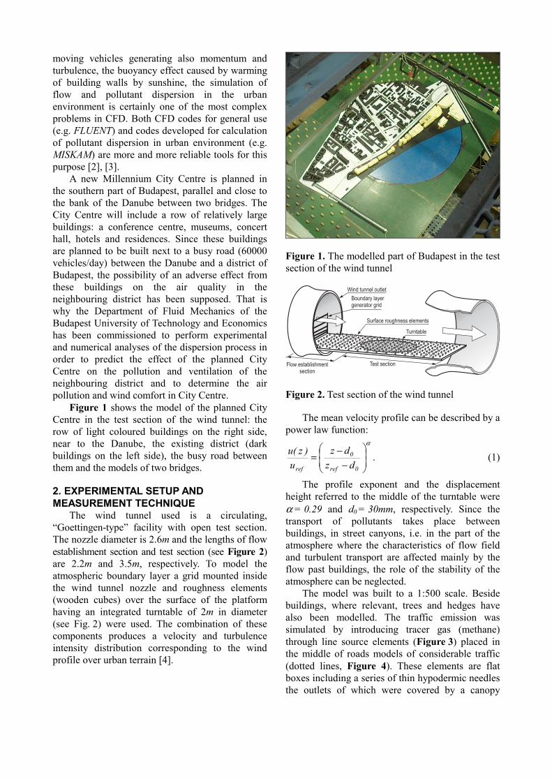
Figure 1 shows the model of the planned City Centre in the test section of the wind tunnel: the row of light coloured buildings on the right side, near to the Danube, the existing district (dark buildings on the left side), the busy road between them and the models of two bridges.

2. EXPERIMENTAL SETUP AND MEASUREMENT TECHNIQUE

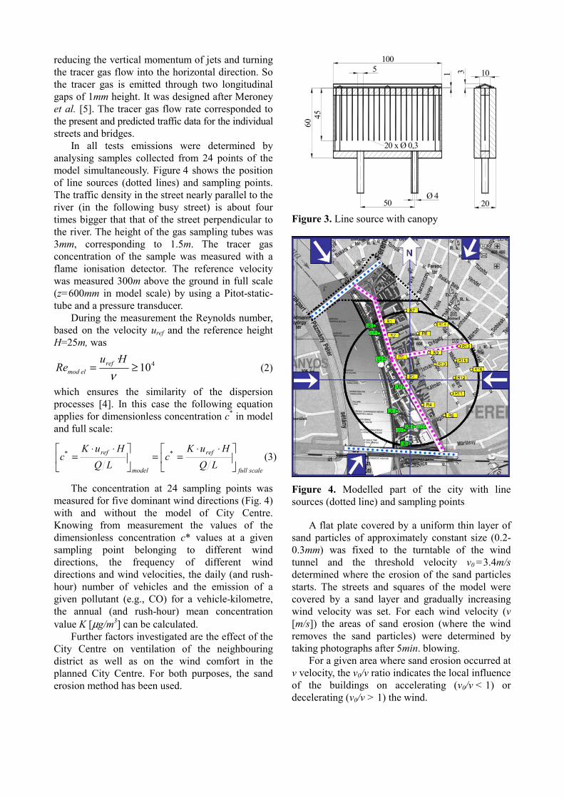
The wind tunnel used is a circulating, “Goettingen-type” facility with open test section. The nozzle diameter is 2.6m and the lengths of flow establishment section and test section (see Figure 2) are 2.2m and 3.5m, respectively. To model the atmospheric boundary layer a grid mounted inside the wind tunnel nozzle and roughness elements (wooden cubes) over the surface of the platform having an integrated turntable of 2m in diameter (see Fig. 2) were used. The combination of these components produces a velocity and turbulence intensity distribution corresponding to the wind profile over urban terrain [4].

Figure 1. The modelled part of Budapest in the test section of the wind tunnel

Wind tunnel outlet

Flow establishmentsection

Test section

Surface roughness elements

Boundary layergenerator grid

Turntable

Figure 2. Test section of the wind tunnel

The mean velocity profile can be described by a power law function:

α

−−

=0ref

0

ref dzdz

u)z(u . (1)

The profile exponent and the displacement height referred to the middle of the turntable were α = 0.29 and d0 = 30mm, respectively. Since the transport of pollutants takes place between buildings, in street canyons, i.e. in the part of the atmosphere where the characteristics of flow field and turbulent transport are affected mainly by the flow past buildings, the role of the stability of the atmosphere can be neglected.

The model was built to a 1:500 scale. Beside buildings, where relevant, trees and hedges have also been modelled. The traffic emission was simulated by introducing tracer gas (methane) through line source elements (Figure 3) placed in the middle of roads models of considerable traffic (dotted lines, Figure 4). These elements are flat boxes including a series of thin hypodermic needles the outlets of which were covered by a canopy

reducing the vertical momentum of jets and turning the tracer gas flow into the horizontal direction. So the tracer gas is emitted through two longitudinal gaps of 1mm height. It was designed after Meroney et al. [5]. The tracer gas flow rate corresponded to the present and predicted traffic data for the individual streets and bridges.

In all tests emissions were determined by analysing samples collected from 24 points of the model simultaneously. Figure 4 shows the position of line sources (dotted lines) and sampling points. The traffic density in the street nearly parallel to the river (in the following busy street) is about four times bigger that that of the street perpendicular to the river. The height of the gas sampling tubes was 3mm, corresponding to 1.5m. The tracer gas concentration of the sample was measured with a flame ionisation detector. The reference velocity was measured 300m above the ground in full scale (z=600mm in model scale) by using a Pitot-static-tube and a pressure transducer.

During the measurement the Reynolds number, based on the velocity uref and the reference height H=25m, was

410≥=ν

H·uRe ref

elmod (2)

which ensures the similarity of the dispersion processes [4]. In this case the following equation applies for dimensionless concentration c* in model and full scale:

scalefull

ref*

model

ref*

LQHuK

cLQ

HuKc

⋅⋅==

⋅⋅= (3)

The concentration at 24 sampling points was measured for five dominant wind directions (Fig. 4) with and without the model of City Centre. Knowing from measurement the values of the dimensionless concentration c* values at a given sampling point belonging to different wind directions, the frequency of different wind directions and wind velocities, the daily (and rush-hour) number of vehicles and the emission of a given pollutant (e.g., CO) for a vehicle-kilometre, the annual (and rush-hour) mean concentration value K [µg/m3] can be calculated.

Further factors investigated are the effect of the City Centre on ventilation of the neighbouring district as well as on the wind comfort in the planned City Centre. For both purposes, the sand erosion method has been used.

100

60

Ø 4

45

5

50

20 x Ø 0,3

1 103

20 Figure 3. Line source with canopy

Figure 4. Modelled part of the city with line sources (dotted line) and sampling points

A flat plate covered by a uniform thin layer of sand particles of approximately constant size (0.2-0.3mm) was fixed to the turntable of the wind tunnel and the threshold velocity v0 =3.4m/s determined where the erosion of the sand particles starts. The streets and squares of the model were covered by a sand layer and gradually increasing wind velocity was set. For each wind velocity (v [m/s]) the areas of sand erosion (where the wind removes the sand particles) were determined by taking photographs after 5min. blowing.

For a given area where sand erosion occurred at v velocity, the v0/v ratio indicates the local influence of the buildings on accelerating (v0/v < 1) or decelerating (v0/v > 1) the wind.

A method was developed to determine the average ventilation of the district under consideration. The sand erosion experiments were carried out at a given wind direction with and without City Centre. For different v0/v values, the areas of sand erosion were summarised by processing the pictures and comparing to the total area of streets and squares of the district model. The change of average ventilation for the district at a given wind direction as a consequence of the planned building can be predicted by comparing the v0/v values with and without City Centre belonging to the same relative area of sand erosion.

3. NUMERICAL SIMULATION OF FLOW AND POLLUTANT TRANSPORT

Calculation of the flow field and concentration distribution was performed with two different codes: MISKAM 4.21 (with and without City Centre) and FLUENT 6.1. (only with City Centre). The micro scale prognostic flow and dispersion model MISKAM solves the 3D equations of motion and the Eulerian dispersion equation for the flow and concentration field in a non-uniform Cartesian grid. The simplified geometrical model of the City Centre taking the orthogonal grid system into consideration and neglecting the accurate modelling of roofs was built up using WinMISKAM 1.94, MISKAM’s user interface [2] (Figure 5). The size of the model domain was 1250m x 1660m x 100m (100 x 100 x 20 cells). Neutral atmosphere was supposed. Wind speed was set to 7 m/s at 100m height. The computational time of a wind direction case was about 3 hours on a 1GHz PC.

The flow and dispersion in City Centre and neighbouring district was also modelled using commercial multipurpose finite volume CFD code FLUENT 6.1. A quite detailed model of the buildings was prepared (Figure 6). Their geometry is complicated, full of critical forms, connections of buildings causing significant problems in preparing it for simulation.

The flow in the wind tunnel model with City Centre building models has been simulated with FLUENT. Because of the special geometrical requirements a non-structured mesh has been created from fully tetrahedral elements. This type of elements provides robust convergence and flexible meshing possibilities. The only disadvantage of this sort of mesh is that the mesh size in the computational domain is not completely controllable.

Figure 5. Modelling the buildings with MISKAM

Figure 6. The model of buildings prepared for FLUENT

The computational domain included one kilometre empty space around the model buildings to avoid direct forcing effects of the boundary conditions. The height of the computational domain was 600mm that is regarding to 300m in full scale. The total computational domain included 978000 cells. The computational time on a 1.8 GHz processor was around one and a half day.

At the inlet, the velocity and the turbulence distribution were specified. These distributions were taken from the wind tunnel experiments. At the outlet of the domain, constant pressure was prescribed as a second order type boundary condition. The sky was represented by a symmetry boundary condition.

„Realizable” k-ε model has been used as turbulence model, which is a vortex viscosity model. The solution of the differential equations has been carried out with the aid of second order upwind difference schemes, and a steady solver called SIMPLE method. With the present settings, the turbulence model has been worked appropriately near the walls, its wall boundary condition requirements were fulfilled, the values of the non-dimensional wall distances y+ was between 30÷500. For the calculations, good convergence was achieved.

The tracer gas has been introduced through volume sources: cells above the given streets were separated from the others and the same amount of methane was introduced as at experiments. So the details of introduction of tracer gas in the wind tunnel model through two gaps between ground and canopy covering the line source (Fig. 3) was not modelled at numerical simulations.

4. RESULTS AND DISCUSSION

4.1. Classification of pollutant transport The transport of pollutants in urban environment

can be modelled with several simple mechanisms. If pollutant source is far from the sampling

point (e.g., the effect of the traffic on the bridges in the district under consideration, see Fig. 6. above) the transport can be called remote source effect.

Figure 7. Demonstration of near source effect

The highest pollutant concentrations arise when the wind transports the pollutant directly from the source to the nearby sampling point: near source effect. Figure 7 shows the result of a simplified 2D flow simulation in the case of wind direction perpendicular to a busy street bounded by buildings only on one side. The concentration distribution shows that the pollutant emitted by the vehicles is directly transported to the downstream pavement and building.

If there are relatively big buildings in the vicinity of the area under consideration, building flow effect can observed. A typical example is the horseshoe vortex accumulating and transporting the pollutants emitted upstream of the building in front and along the sides [6]. Another effect can be seen in Figure 8 where the concentration distribution is shown in the case of the same busy street as in Fig. 7, but with large buildings on the upstream side of it. If the pollutant is emitted in the wake of a building, the wake flow elevates the pollutants and so, near the ground, the downstream concentration will be reduced.

In the case of a street canyon (where two rows of buildings bound the street) the transport of pollutants is mainly affected by two mechanisms and their combinations: by street channel effect

and street vortex effect [7]. If the angle between wind velocity and the axis of the street is smaller than about 30°, the flow will be “channelled” by the buildings, i.e. flow along the street will arise, accumulating the pollutants. In this case, continuous increase of concentration can be observed in the wind direction along the street. Figure 9 shows the change of dimensionless concentration c* defined by Eq. (3) at 4 sampling points along the street in wind direction (R1-R4 sampling points, see Fig. 4.).

Figure 8. The building elevates the pollutants

0

10

20

30

40

50

60

R1 R2 R3 R4

c*

R1

R2

R3

R4

without CC

with CC

Figure 9. Change of concentration along a street (wind direction NW-NNW)

In the left diagram the grey bars show the c* values without, the black ones with City Centre determined from wind tunnel experiments. In the former case, when the busy street was bounded only by one row of building, the increase of pollutant concentration is quite modest: the pollutants can expand in the direction of empty building sites.

This expansion of pollution can be clearly seen on the right side of Fig. 9 where the dimensionless concentration distribution is shown (simulated with Fluent) in a horizontal plane 1.5m high above the ground, after construction of City Centre. There is an empty area in the lower part of the right side of the busy street where no buildings hinder the expansion of flow which is accompanied by a reduction of local wind velocity and an increase of concentration.

Because of the wide range (two orders of magnitude) of concentration both here and in similar concentration distribution diagrams, the logarithm of the concentration is shown. Due to the street channel effect, the increase of concentration along the street is more rapid after construction of the City Centre (see black bars and concentration distribution in Fig. 9.)

If the wind direction is nearly perpendicular to the street canyon a vortex arises whose axis is parallel to that of the street, carrying pollutants towards the upstream side of the street (see Figure 10). This effect causes a substantial concentration gradient across the street: the ratio of upstream and downstream side concentration reaches 5:1 [7]. In most cases, the street channel and vortex effects are combined.

Figure 10. Street vortex and its effect on the concentration distribution across a street

4.2. Results of concentration measurements Through a series of measurements the effect of the

planned City Centre on the concentration at sampling points shown in Fig. 4 has been investigated. The main results of the measurements are as follows:

a) The concentration increase caused by remote source effect is relatively modest: the quite busy Petőfi bridge (70.000 vehicle/day, see Fig. 4 upper bridge) causes only 5% increase in sampling points in the busy street which are about 0.5 - 1 km away from the bridge. This indicates a quite rapid dilution of the pollutants due to the turbulent diffusion. In sampling points inside the district and the City Centre far from the traffic related emission (where the concentration is only few percent of that of sampling points in the busy street) the effect of the traffic on the bridge was quite considerable.

0

10

20

30

40

50

R1 R3 R5 R7 R9 R11 R13 R15 U1 U3 U5 U7 U9measuring points

c*

without CC

with CC

Figure 11. Concentration distribution and effect of City Centre a SW-SSW wind direction

b) Figure 11 shows the result of numerical simulation of concentration distribution at SW-SSW wind direction in a plane 1.5m above the ground. When analysing the concentration distribution a number of pollution transport effects can be recognised in different parts of the district. When comparing the dimensionless concentration measured in different sampling points with (black bars) and without (grey bars) City Centre the sampling points can be divided into two parts: the sampling points in the busy street exposed to immediate effect of traffic emission (the first four bars and four out of the last five bars) and the rest of the sampling points situated in the inner part of the district and the city centre (see Fig. 4).

In the former sampling points the concentration is high and it is very much influenced by the buildings. While in the case of wind direction NW-NNW (Fig. 9) the City Centre increased the concentration along the busy street because of enhancing street channel effect, at SW-SSW wind direction (Fig. 11) the buildings reduced the concentration by stopping the near source effect and generating the street vortex effect. It is remarkable

that clean air “jets” flowing out of the streets between the City Centre buildings cause low concentration areas locally in the busy street, too.

In the points inside the district and the City Centre far from the busy street the concentration is by 1-2 orders of magnitude smaller and it is influenced via combined building flow and remote source effects by the buildings of City Centre.

c) The effect of City Centre on the annual mean CO concentration K [µg/m3] is shown in Figure 12, determined from the measured dimensionless concentration c* in sampling points belonging to different wind directions, the frequency of different wind directions and wind velocities, the daily number of vehicles and the CO emission for 1 vehicle-kilometre.

0

2

4

6

8

R1 R3 R5 R7 R9 R11 R13 R15 U1 U3 U5 U7 U9measuring points

K /

Kor

ig. m

ean

without CC

with CC

Figure 12. The effect of the City Centre on the annual mean CO concentration

On the basis of the measurements, a reduction of the air pollution in the district under consideration (sampling points R1-R16) can be predicted. In the internal part of the district the change is negligible but in the busy street (sampling points R1-R4) the overall concentration reduction is 14%. These results include also the considerable (about 20%) increase of the traffic caused by the City Centre, too.

4.3. Comparison of measurement and simulation

When comparing the results of simulation and measurements in the case of MISKAM the concentration value belonging to the cell coinciding with the sampling point has been taken. In the case of FLUENT the spatial change of concentration has been substantial, particularly in points close to the emission source cells. That is why in presenting the results of FLUENT simulation the concentration is determined differently. Concentration distribution has been plotted along the line of the cross section

perpendicular to the street, including the sampling point, 1.5m over the ground. By taking the maximum and minimum values of this concentration distribution, a concentration interval has been defined for all sampling points.

In order to compare the wind tunnel and CFD results the measured and calculated concentrations have been plotted as a function of wind direction. One example is shown for a sampling point far from pollutant sources in the interior of the district (Figure 13).

0

0.5

1

1.5

2

2.5

3

0 60 120 180 240 300 360

Wind direction [deg]

MISKAM 4.21

Wind Tunnel

FLUENT 6(min&max. values in

the street cross-section)

c*

Figure 13. Measured and calculated dimensionless concentration plotted against wind direction for sampling point R10.

For a sampling point far from the pollutant source shown in Fig. 13., the concentration calculated with FLUENT does not change too much across the street. There are considerable differences between measured and calculated concentration values but the trends of change reflected by both simulations are in general correctly. In the case of sampling points close to the pollution source, the differences between measured and calculated values and the change of concentration across the street are in general larger. The differences can partly be explained by the inaccurate modelling of tracer gas release in numerical simulation.

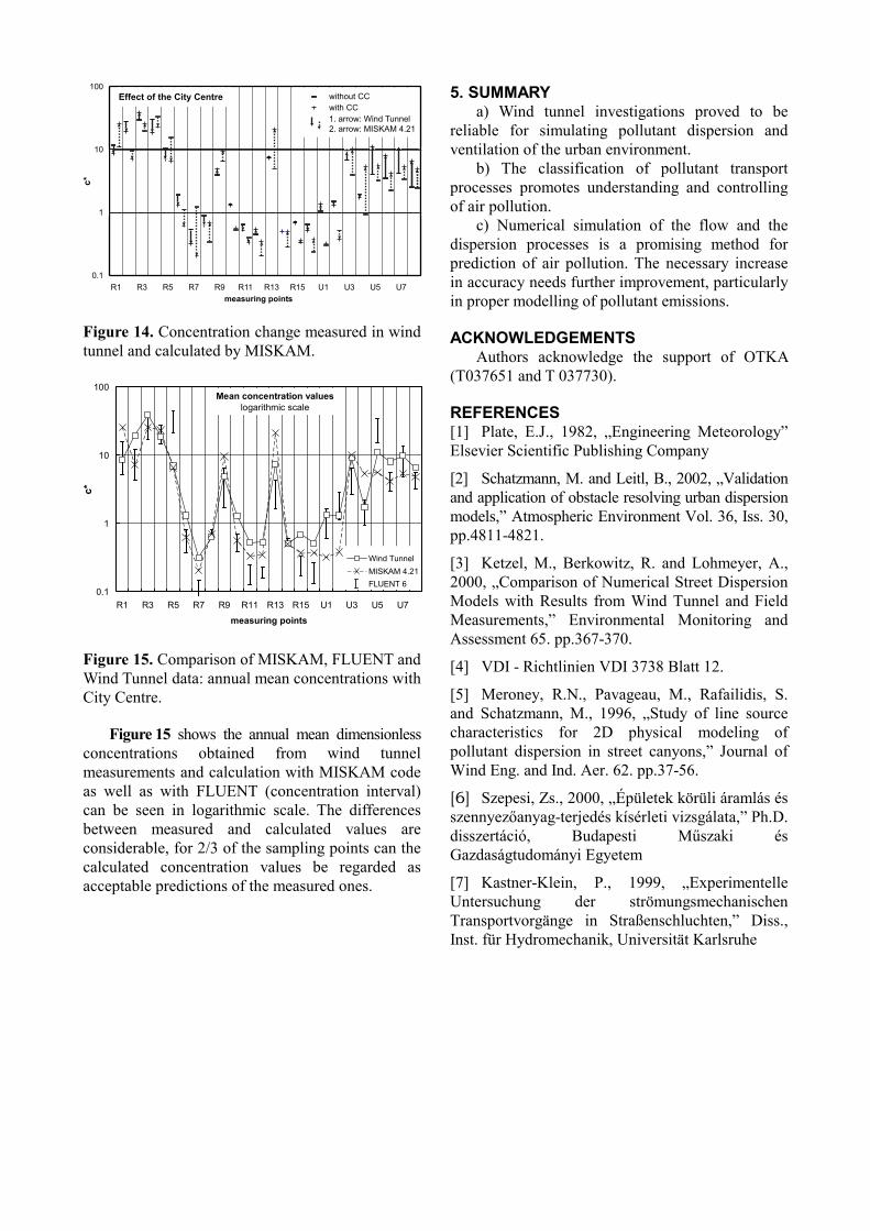
Considering the probabilities of wind directions the annual mean dimensionless concentration can be calculated for every sampling point. Figure 14 shows two arrows in each sampling point. They show the measured and calculated change of annual mean dimensionless concentration caused by the City Centre. It can be seen that the agreement of measured and calculated mean values is in most cases quite acceptable and the trends of change caused by City Centre are correctly predicted in 3/4 of sampling point.

Effect of the City Centre

0.1

1

10

100

R1 R3 R5 R7 R9 R11 R13 R15 U1 U3 U5 U7

measuring points

c*

without CC

with CC

1. arrow: Wind Tunnel

2. arrow: MISKAM 4.21

Figure 14. Concentration change measured in wind tunnel and calculated by MISKAM.

Mean concentration valueslogarithmic scale

0.1

1

10

100

R1 R3 R5 R7 R9 R11 R13 R15 U1 U3 U5 U7

measuring points

c*

Wind TunnelMISKAM 4.21FLUENT 6

Figure 15. Comparison of MISKAM, FLUENT and Wind Tunnel data: annual mean concentrations with City Centre.

Figure 15 shows the annual mean dimensionless concentrations obtained from wind tunnel measurements and calculation with MISKAM code as well as with FLUENT (concentration interval) can be seen in logarithmic scale. The differences between measured and calculated values are considerable, for 2/3 of the sampling points can the calculated concentration values be regarded as acceptable predictions of the measured ones.

5. SUMMARY a) Wind tunnel investigations proved to be

reliable for simulating pollutant dispersion and ventilation of the urban environment.

b) The classification of pollutant transport processes promotes understanding and controlling of air pollution.

c) Numerical simulation of the flow and the dispersion processes is a promising method for prediction of air pollution. The necessary increase in accuracy needs further improvement, particularly in proper modelling of pollutant emissions.

ACKNOWLEDGEMENTS Authors acknowledge the support of OTKA

(T037651 and T 037730).

REFERENCES [1] Plate, E.J., 1982, „Engineering Meteorology” Elsevier Scientific Publishing Company

[2] Schatzmann, M. and Leitl, B., 2002, „Validation and application of obstacle resolving urban dispersion models,” Atmospheric Environment Vol. 36, Iss. 30, pp.4811-4821.

[3] Ketzel, M., Berkowitz, R. and Lohmeyer, A., 2000, „Comparison of Numerical Street Dispersion Models with Results from Wind Tunnel and Field Measurements,” Environmental Monitoring and Assessment 65. pp.367-370.

[4] VDI - Richtlinien VDI 3738 Blatt 12.

[5] Meroney, R.N., Pavageau, M., Rafailidis, S. and Schatzmann, M., 1996, „Study of line source characteristics for 2D physical modeling of pollutant dispersion in street canyons,” Journal of Wind Eng. and Ind. Aer. 62. pp.37-56.

[6] Szepesi, Zs., 2000, „Épületek körüli áramlás és szennyezőanyag-terjedés kísérleti vizsgálata,” Ph.D. disszertáció, Budapesti Műszaki és Gazdaságtudományi Egyetem

[7] Kastner-Klein, P., 1999, „Experimentelle Untersuchung der strömungsmechanischen Transportvorgänge in Straßenschluchten,” Diss., Inst. für Hydromechanik, Universität Karlsruhe