wind turbine rotors with active vibration control - dtu …orbit.dtu.dk/files/6314637/s122 martin...
TRANSCRIPT

General rights Copyright and moral rights for the publications made accessible in the public portal are retained by the authors and/or other copyright owners and it is a condition of accessing publications that users recognise and abide by the legal requirements associated with these rights.
• Users may download and print one copy of any publication from the public portal for the purpose of private study or research. • You may not further distribute the material or use it for any profit-making activity or commercial gain • You may freely distribute the URL identifying the publication in the public portal
If you believe that this document breaches copyright please contact us providing details, and we will remove access to the work immediately and investigate your claim.
Downloaded from orbit.dtu.dk on: Jun 28, 2018
Wind Turbine Rotors with Active Vibration Control
Svendsen, Martin Nymann; Krenk, Steen; Høgsberg, Jan Becker
Publication date:2011
Document VersionPublisher's PDF, also known as Version of record
Link back to DTU Orbit
Citation (APA):Svendsen, M. N., Krenk, S., & Høgsberg, J. B. (2011). Wind Turbine Rotors with Active Vibration Control. Kgs.Lyngby, Denmark: Technical University of Denmark (DTU). (DCAMM Special Report; No. S122).
Wind Turbine Rotors with Active Vibration Control
Ph
D T
he
sis
Martin Nymann SvendsenDCAMM Special Report No. S122Januar 2011

Wind Turbine Rotors with Active Vibration
Control
Martin Nymann Svendsen
TECHNICAL UNIVERSITY OF DENMARK
DEPARTMENT OF MECHANICAL ENGINEERING
SECTION OF COASTAL, MARITIME AND STRUCTURAL ENGINEERING
MARCH 2011

Published in Denmark byTechnical University of Denmark
Copyright c© M. N. Svendsen 2011
All rights reserved
Section of Coastal, Maritime and Structural EngineeringDepartment of Mechanical EngineeringTechnical University of DenmarkNils Koppels Alle, Building 403, DK-2800 Kgs. Lyngby, DenmarkPhone +45 4525 1360, Telefax +45 4588 4325E-mail: [email protected]: http://www.mek.dtu.dk/
Publication Reference Data
Svendsen, M. N.Wind Turbine Rotors with Active Vibration ControlPhD ThesisTechnical University of Denmark, Section of Coastal, Mar-itime and Structural Engineering.March, 2011ISBN 978-87-90416-42-3Keywords: Active vibration control, resonant control, finite
beam element, rotating beams, rotor dynamics,whirling modes, wind turbine control, gyroscopicsystems, aeroelastic modeling

Abstract
This thesis presents a framework for structural modeling, analysis and active vibra-tion damping of rotating wind turbine blades and rotors. A structural rotor modelis developed in terms of finite beam elements in a rotating frame of reference. Theelement comprises a representation of general, varying cross-section properties and as-sumes small cross-section displacements and rotations, by which the associated elasticstiffness and inertial terms are linear. The formulation consistently describes all in-ertial terms, including centrifugal softening and gyroscopic forces. Aerodynamic liftforces are assumed to be proportional to the relative inflow angle, which also gives alinear form with equivalent stiffness and damping terms. Geometric stiffness effectsincluding the important stiffening from tensile axial stresses in equilibrium with cen-trifugal forces are included via an initial stress formulation. The element provides anaccurate representation of the eigenfrequencies and whirling modes of the gyroscopicsystem, and identifies lightly damped edge-wise modes. By adoption of a method foractive, collocated resonant vibration of multi-degree-of-freedom systems it is demon-strated that the basic modes of a wind turbine blade can be effectively addressedby an in-blade ‘active strut’ actuator mechanism. The importance of accounting forbackground mode flexibility is demonstrated. Also, it is shown that it is generallypossible to address multiple beam modes with multiple controllers, given that theseare geometrically well separated. For active vibration control in three-bladed windturbine rotors the present work presents a resonance-based method for groups of onecollective and two whirling modes. The controller is based on the existing resonantformat and introduces a dual system targeting the collective mode and the combinedwhirling modes respectively, via a shared set of collocated sensor/actuator pairs. Thecollective mode controller is decoupled from the whirling mode controller by an ex-act linear filter, which is identified from the fundamental dynamics of the gyroscopicsystem. As in the method for non-rotating systems, an explicit procedure for opti-mal calibration of the controller gains is established. The control system is appliedto an 86m wind turbine rotor by means of active strut actuator mechanisms. Theprescribed additional damping ratios are reproduced almost identically in the tar-geted modes and the observed spill-over to other modes is very limited and generallystabilizing. It is shown that physical controller positioning for reduced backgroundnoise is important to the calibration. By simulation of the rotor response to bothsimple initial conditions and a stochastic wind load it is demonstrated that the am-plitudes of the targeted modes are effectively reduced, while leaving the remainingmodes virtually unaffected.
i

Resume
I denne afhandling præsenteres en metoderamme for modellering, analyse og aktivvibrationsdæmpning af roterende vindmølleblade og rotorer. En strukturel modeludvikles i form af rumlige bjælkelementer i en roterende referenceramme. Elementetindeholder en repræsentation af generelle, varierende tværsnitsegenskaber og antagersma tværsnitsflytninger og rotationer, hvorved de tilhørende elastiske led og iner-tialled bliver lineære. Formuleringen beskriver pa konsistent vis alle inertialled, inklu-siv negativ centrifugalstivhed og gyroskopiske kræfter. Aerodynamisk lift antages atvære proportionalt til den relative indfaldsvinkel, hvilket ogsa giver en lineær formmed ækvivalente stivheds- og dæmpningsled. Geometriske stivhedseffekter, herunderdet vigtige stivhedsbidrag fra trækspændinger i ligevægt med centrifugalbelastnin-gen, er inkluderede via en initialspændingsformulering. Elementet giver en præcisrepresentation af egenfrekvenser og hvirvlende svingningsformer i det gyroskopiskesystem, og lavt aerodynamisk dæmpede kantvise svingningsformer identificeres. Vedindførelse af en metode for aktiv, kollokeret, resonansbaseret vibrationskontrol affler-frihedsgradssystemer demonstreres det, at de grundlæggende svingningsformer afet isoleret vindmølleblad effektivt kan dæmpes via en aktiv trækstangsmekanisme.Vigtigheden af at inkludere effekten af modal baggrundsfleksibilitet demonstreres.Det vises endvidere at det er muligt at addressere flere svingningsformer med flereseparate kontrolsystemer, nar formerne er geometrisk vel adskilt. Til aktiv vibra-tionskontrol i trebladede vindmøllerotorer præsenteres en resonansbaseret metode,malrettet grupper bestaende af en kollektiv og to hvivlende svingningsformer. Kon-trolsystemet er baseret pa det kendte format og introducerer et dobbelt format somadresserer henholdsvis den kollektive og de hvirvlende svingningsformer, via et deltsæt af kollokerede sensor/aktuator par. Kontroldelen til den kollektive svingningsformer afkoblet fra kontroldelen til de hvirvlende svingningsformer via et eksakt lineærtfilter der er identificeret pa baggrund af det gyroskopiske systems grundlæggendedynamik. Som i metoden for ikke-roterende systemer etableres en eksplicit kali-breringsprocedure. Kontrolsystemet anvendes pa en 86m vindmøllerotor via aktivetrykstænger. De foreskrevne supplerende dæmpningsforhold reproduceres næstenidentisk i de adresserede svingningsformer og den observerede interaktion med andresvingningsformer er meget begrænset og generelt stabiliserende. Det vises at fysiskpositionering af kontrolsystemet for reduceret baggrundsflexibilitet er vigtigt for kali-breringen. Ved simulering af rotorens respons til bade simple begyndelsesbetingelserog et stokastisk vindfelt demonstreres det, at amplituderne af de adresserede svingn-ingsformer effektivt reduceres, mens de øvrige svingninger nærmest ikke pavirkes.
ii

Preface
This thesis is submitted in partial fulfilment of the Ph.D. degree from the TechnicalUniversity of Denmark. The work has primarily been performed at the Departmentof Mechanical Engineering at the Technical University of Denmark, in the periodJanuary 2008 to January 2011. The study has been performed under the supervisionof Professor Dr. Techn. Steen Krenk as main supervisor and Associate ProfessorJan Høgsberg as co-supervisor. I owe my deepest gratitude to Steen Krenk and JanHøgsberg for their excellent guidance and support throughout the entire project.
The project is part of the Danish Industrial PhD programme and part of the workhas been carried out at Vestas Wind Systems A/S under the supervision of RasmusSvendsen and Per Brath. I would like to express my gratitude to both for their supportand inspiring enthusiasm. The financing from the Danish Agency for Science, Tech-nology and Innovation and Vestas Wind Systems A/S is also gratefully acknowledged.
Finally, I would like to express my most sincere thanks to those close to me for theirpatience and support. And, in particular, Maria, for being always encouraging andunderstanding.
Martin Nymann Svendsen
Copenhagen, January 2011
iii

Publications
Appended papers
[P1] M.N. Svendsen, S. Krenk, J. Høgsberg,
Resonant vibration control of rotating beams,
Journal of Sound and Vibration, (2010), (doi:10.1016/j.jsv.2010.11.008).
[P2] M.N. Svendsen, S. Krenk, J. Høgsberg,
Resonant vibration control of wind turbine blades,
TORQUE 2010: The Science of Making Torque from Wind, 543–553,
June 28–30, Creete, Greece, 2010.
[P3] S. Krenk, M.N. Svendsen, J. Høgsberg,
Resonant vibration control of three-bladed wind turbine rotors,
(2011), Paper submitted.
Other Contributions
M.N. Svendsen, S. Krenk, J. Høgsberg,
Resonant vibration control of beams under stationary rotation,
Proceedings of the Twenty Second Nordic Seminar on Computational Mechanics, 75–78,
October 22–23, Aalborg, Denmark, 2009.
iv
Contents
1 Introduction 1
2 Rotating Finite Beam Element 5
2.1 Inertial Effects . . . . . . . . . . . . . . . . . . . . . . . . . . . . . . . . . . . 5
2.1.1 Beam Kinematics . . . . . . . . . . . . . . . . . . . . . . . . . . . . . . 6
2.1.2 Kinetic Energy . . . . . . . . . . . . . . . . . . . . . . . . . . . . . . . 7
2.1.3 Inertial Matrices . . . . . . . . . . . . . . . . . . . . . . . . . . . . . . 8
2.2 Stiffness Effects . . . . . . . . . . . . . . . . . . . . . . . . . . . . . . . . . . . 10
2.2.1 Elastic Stiffness . . . . . . . . . . . . . . . . . . . . . . . . . . . . . . . 10
2.2.2 Geometric Stiffness . . . . . . . . . . . . . . . . . . . . . . . . . . . . . 13
2.3 Aerodynamic Effects . . . . . . . . . . . . . . . . . . . . . . . . . . . . . . . . 15
2.3.1 Angle of Attack . . . . . . . . . . . . . . . . . . . . . . . . . . . . . . . 15
2.3.2 Aerodynamic Forces . . . . . . . . . . . . . . . . . . . . . . . . . . . . 17
2.4 Equations of Motion . . . . . . . . . . . . . . . . . . . . . . . . . . . . . . . . 18
2.4.1 Conservative Terms via Lagrange’s Equations . . . . . . . . . . . . . . 18
2.4.2 Non-Conservative Aerodynamic Terms via Virtual Work . . . . . . . . 19
2.4.3 Aeroelastic Equations of Motion . . . . . . . . . . . . . . . . . . . . . 20
2.4.4 Beam Element Integration . . . . . . . . . . . . . . . . . . . . . . . . . 21
2.5 Modal Analysis for Stationary Rotation . . . . . . . . . . . . . . . . . . . . . 23
2.5.1 State-Space Formulation . . . . . . . . . . . . . . . . . . . . . . . . . . 24
2.5.2 Eigensolution Analysis . . . . . . . . . . . . . . . . . . . . . . . . . . . 24
2.5.3 Frequency Response Analysis . . . . . . . . . . . . . . . . . . . . . . . 25
3 Rotor Systems in Finite Elements 27
3.1 Rotor Assembly and Simulation . . . . . . . . . . . . . . . . . . . . . . . . . . 27
3.1.1 Finite Element Rotor Model Assembly . . . . . . . . . . . . . . . . . . 28
3.1.2 Integration of Rotor Equations of Motion . . . . . . . . . . . . . . . . 29
3.2 Example: 8m Prismatic Rotor Blade . . . . . . . . . . . . . . . . . . . . . . . 31
3.2.1 The Rotor Blade . . . . . . . . . . . . . . . . . . . . . . . . . . . . . . 33
3.2.2 Modal Analysis . . . . . . . . . . . . . . . . . . . . . . . . . . . . . . . 33
3.2.3 Spin-Up Maneuver . . . . . . . . . . . . . . . . . . . . . . . . . . . . . 34
3.3 Example: Aeroelastic Analysis of a 42m Wind Turbine Blade . . . . . . . . . 37
3.3.1 Structural Properties . . . . . . . . . . . . . . . . . . . . . . . . . . . . 37
3.3.2 Static Analysis . . . . . . . . . . . . . . . . . . . . . . . . . . . . . . . 39
3.3.3 Modal Analysis . . . . . . . . . . . . . . . . . . . . . . . . . . . . . . . 41
3.4 Dynamics of Three-Bladed Rotors . . . . . . . . . . . . . . . . . . . . . . . . 44
3.4.1 Vibration Modes . . . . . . . . . . . . . . . . . . . . . . . . . . . . . . 45
3.4.2 Dynamics of Whirling . . . . . . . . . . . . . . . . . . . . . . . . . . . 46
3.5 Example: Simulation of 86m Wind Turbine Rotor . . . . . . . . . . . . . . . 49
3.5.1 Modal Analysis . . . . . . . . . . . . . . . . . . . . . . . . . . . . . . . 49
3.5.2 Free Vibration . . . . . . . . . . . . . . . . . . . . . . . . . . . . . . . 51
v
4 Resonant Vibration Control of Beams and Rotors 544.1 Basic Idea of the Resonant Controller . . . . . . . . . . . . . . . . . . . . . . 544.2 Control of Rotating Beams . . . . . . . . . . . . . . . . . . . . . . . . . . . . 56
4.2.1 Controller Format . . . . . . . . . . . . . . . . . . . . . . . . . . . . . 564.2.2 Example: Control of 42m Wind Turbine Blade . . . . . . . . . . . . . 57
4.3 Control of Three-Bladed Rotors . . . . . . . . . . . . . . . . . . . . . . . . . . 594.3.1 Controller Format . . . . . . . . . . . . . . . . . . . . . . . . . . . . . 604.3.2 Example: Control of 86m Wind Turbine Rotor . . . . . . . . . . . . . 61
5 Conclusions 66
Bibliography 67
A Matrices 70A.1 Shape Functions . . . . . . . . . . . . . . . . . . . . . . . . . . . . . . . . . . 70A.2 Cross-section Inertia . . . . . . . . . . . . . . . . . . . . . . . . . . . . . . . . 71
B Alternative Beam Kinematics 73B.1 Kinematics with Shear and Elastic Center . . . . . . . . . . . . . . . . . . . . 73B.2 Elastic Stiffness . . . . . . . . . . . . . . . . . . . . . . . . . . . . . . . . . . . 74B.3 Geometric Stiffness . . . . . . . . . . . . . . . . . . . . . . . . . . . . . . . . . 75
C Collocated Sensor/Actuator Connectivity 77
D Algorithms 79D.1 Element Integration . . . . . . . . . . . . . . . . . . . . . . . . . . . . . . . . 79D.2 Rotor Assembly and Simulation . . . . . . . . . . . . . . . . . . . . . . . . . . 80
vi
Chapter 1
Introduction
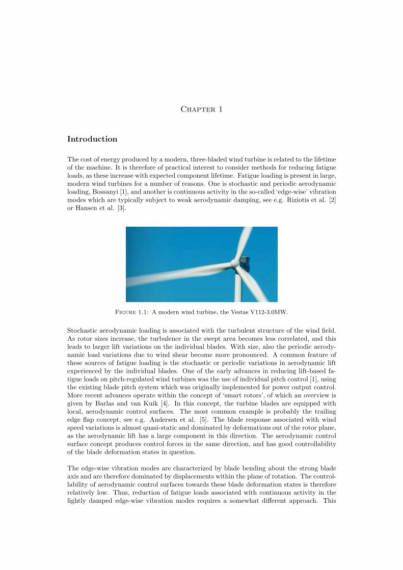
The cost of energy produced by a modern, three-bladed wind turbine is related to the lifetimeof the machine. It is therefore of practical interest to consider methods for reducing fatigueloads, as these increase with expected component lifetime. Fatigue loading is present in large,modern wind turbines for a number of reasons. One is stochastic and periodic aerodynamicloading, Bossanyi [1], and another is continuous activity in the so-called ‘edge-wise’ vibrationmodes which are typically subject to weak aerodynamic damping, see e.g. Riziotis et al. [2]or Hansen et al. [3].
Figure 1.1: A modern wind turbine, the Vestas V112-3.0MW.
Stochastic aerodynamic loading is associated with the turbulent structure of the wind field.As rotor sizes increase, the turbulence in the swept area becomes less correlated, and thisleads to larger lift variations on the individual blades. With size, also the periodic aerody-namic load variations due to wind shear become more pronounced. A common feature ofthese sources of fatigue loading is the stochastic or periodic variations in aerodynamic liftexperienced by the individual blades. One of the early advances in reducing lift-based fa-tigue loads on pitch-regulated wind turbines was the use of individual pitch control [1], usingthe existing blade pitch system which was originally implemented for power output control.More recent advances operate within the concept of ‘smart rotors’, of which an overview isgiven by Barlas and van Kuik [4]. In this concept, the turbine blades are equipped withlocal, aerodynamic control surfaces. The most common example is probably the trailingedge flap concept, see e.g. Andersen et al. [5]. The blade response associated with windspeed variations is almost quasi-static and dominated by deformations out of the rotor plane,as the aerodynamic lift has a large component in this direction. The aerodynamic controlsurface concept produces control forces in the same direction, and has good controllabilityof the blade deformation states in question.
The edge-wise vibration modes are characterized by blade bending about the strong bladeaxis and are therefore dominated by displacements within the plane of rotation. The control-lability of aerodynamic control surfaces towards these blade deformation states is thereforerelatively low. Thus, reduction of fatigue loads associated with continuous activity in thelightly damped edge-wise vibration modes requires a somewhat different approach. This

2 Introduction
work presents an active vibration control method for introducing damping to the first groupof edge-wise vibration modes of three-bladed wind turbine rotors, Krenk et al. [6]. Thegroup consists of three modes, namely the collective mode where all blades vibrate in phaseand thereby activate the torsional flexibility of the main rotor shaft, and the backward andforward whirling modes which activate the transverse flexibility of the rotor shaft. The ac-tuator system is based on assumed in-blade mechanisms, capable of imposing local bendingmoments. An example is shown in Fig. 1.2 where an active strut, see e.g. Preumont etal. [7], is positioned near the blade root with attachment points at the two shown cross-sections. By contraction or elongation the strut imposes a bending moment about the localblade y-axis. This gives good controllability of the edge-wise modes.
x
y
z
Qη
−Qη
Figure 1.2: An active strut applied to a wind turbine blade.
As opposed to the somewhat quasi-static nature of the out-of-plane blade deformation prob-lem, the targeted modal edge-wise response is purely dynamic. For this reason the presentactive control system is based on resonant interaction with the flexible structure. An earlyexample of a passive, resonant vibration control system is the tuned mass damper, Ormon-droyd & Den Hartog [8] which was originally designed for application to a single-degree-freedom-system. One of the pioneering works addressing modal vibrations in flexible, con-tinuous structures was performed by Meirovitch [9] in terms of the ‘independent modal spacecontrol’ formulation. A formulation for active damping of one or more selected modes withzero spill-over was given, provided that a distributed sensor/actuator system is available.A more practical form of the modal control concept was given by Balas [10] in terms of afeedback controller with a finite number of discrete sensors and actuators. This work alsointroduced the use of modal state observers and gain calibration according to the theoryof optimal linear quadratic control. Furthermore the concepts of modal observability andcontrollability were introduced, along with the concepts of observation and control spill-overand associated closed-loop instability issues.
The amount of relevant literature concerning resonant vibration control for three-bladedrotors appears limited. Also, the application of active resonant control to rotating systemsin general seems limited. Recent investigations on vibration control of isolated, rotatingbeams have primarily focused on the use of novel smart materials, implementing well estab-lished control algorithms, such as direct velocity feedback, Choi et al. [11] or optimal linearquadratic control based on either estimated modal states, Khulief [12] or physical systemstates, see e.g. Shete et al. [13] or Chandiramani [14]. The present control method is basedon the active, collocated resonant controller format given by Krenk & Høgsberg [15, 16].Here an explicit calibration scheme was given for the controller filters, including a correctionfor the quasi-static flexibility of higher modes of multi-degree-of-freedom structure. Themethod was adopted for application to an isolated wind turbine blade in Svendsen et al.[17, 18] and the explicit calibration scheme provided almost optimal tuning and performanceof the control system.
The rotor control method is based on a dual controller system targeting the collectivemode and the whirling modes, respectively. The controllers interact with the rotor viaa shared set of collocated sensor/actuator pairs. The whirling mode controller introduces a

3
multi-component format which is necessary to control the out-of-phase motion of the threeblades associated with whirling. For calibration, the coupled system of multi-degree-of-freedom structural equations and multi-component controller equations are collapsed intoscalar modal equations analogous to those of the basic resonant system of [15, 16], and theoptimal filter parameters are identified by comparison. As input, the explicit calibrationprocedure takes the desired additional damping ratios, eigenfrequencies and complex-valuedmode shapes of the targeted modes. Also, the physical connectivity of the collocated sen-sor/actuator configuration is used. As such, the calibration of the control system is basedentirely on the properties of the targeted modes. The controller operates with a discreteacceleration feedback measured directly from the physical rotor deformation states. Thus,the operating controller makes no use of model reduction techniques or (modal) state ob-servers. A concise proof of closed-loop stability and robustness has not been established,but the aforementioned features renders its existence probable.
As an example, the control system is applied to an 86m wind turbine rotor using symmet-rically positioned active struts as shown in Fig. 1.3. It is demonstrated by modal analysisof the closed-loop system that the calibration procedure provides the intended additionaldamping to the desired modes, with insignificant spill-over. Time integration of the rotorresponse to a simulated turbulent wind field, Krenk et al. [6], furthermore demonstratesthat the control system effectively reduces the targeted modal vibration amplitudes in astochastic environment.
x
y
z
Figure 1.3: Three-bladed wind turbine rotor with actuator struts.
The wind turbine rotor is modeled using finite beam elements in a rotating frame of refer-ence, Svendsen et al. [17, 18]. The element comprises a representation of general, varyingcross-section properties including e.g. the positions of the elastic, shear and mass centers.The formulation assumes small cross-section displacements and rotations, by which the as-sociated elastic stiffness and inertial terms are linear. Aerodynamic lift and drag forces areassumed to be proportional to the relative inflow angle, which also gives a linear form withequivalent stiffness and damping terms for small relative angle changes. Geometric stiffnesseffects are included via an initial stress formulation based on the undeformed structuralgeometry. This gives a linear stiffness contribution in terms of initial cross-section forcesand moments. In the present application no initial stresses are present, and the formulationis intended to approximate the effects from current stresses due to aerodynamic and inertialloads. These are treated as initial stresses and the associated geometric stiffness effectsare computed based on the undeformed structural geometry. The use of current stresses

4 Introduction
introduces a non-linearity in the model, as the balance between structural deformation andequivalent stiffness due to internal stresses must be established by iteration. For stationaryangular velocity of the rotor and no turbulence the structural equations of motion haveconstant terms and modal analysis can be performed following e.g. Geradin & Rixen [19].For frequency response analysis of the gyroscopic system a formulation which captures boththe symmetric contribution due to non-rotating effects and the skew-symmetric gyroscopiceffects is used, Krenk et al. [6].
The text is organized as follows. In Chapter 2 the assumed beam kinematics is presented andthe gyroscopic, aeroelastic equations of motion with geometric stiffness effects are derivedfor the finite beam element in a rotating frame of reference. The element matrices and loadvectors appear in integral form and the used method for evaluation by Gaussian quadratureis presented. Finally, a framework for modal analysis and frequency response analysis of thegyroscopic system is given. Elements of the rotor model assembly and simulation proceduresare initially given in Chapter 3. The fundamental dynamic features of three-bladed rotorsare subsequently illustrated by a few numerical examples, and the dynamics of whirlingare discussed in detail. Chapter 4 is initiated by a presentation of the basic format of aresonant controller. This is followed by an overview of the adopted formulation for multi-degree-of-freedom structures, and an example of application to a 42m wind turbine bladeis given, using the active strut actuator mechanism. The first flap-wise mode and the firstedge-wise mode are addressed and the issue of optimal controller positioning is addressed.Subsequently, an overview of the control system format for flexible, three-bladed rotors isgiven. The numerical example with application to an 86m rotor then follows. The exampleincludes a discussion of the implications of physical sensor/actuator positioning and a simpletime simulation example is given to present the fundamental function of the controller. InChapter 5 the primary developments of the presented work are summarized.

Chapter 2
Rotating Finite Beam Element
The wind turbine rotor consists of three flexible blades connected in a common flexiblesupport point, and can in this sense be seen as a system of rotating beam-like structures.The present resonant vibration control formulation for flexible three-bladed rotors is definedin terms of a finite element representation of the targeted structure, and in this chaptera consistent three-dimensional finite element formulation for beams in a rotating frame ofreference is developed. Geometric stiffness effects including the important stiffening fromtensile axial stresses in equilibrium with centrifugal forces are included via an initial stressformulation and the inertial terms capture the gyroscopic forces which are essential in therepresentation of whirling modes. A simple aerodynamic formulation is included to allow arealistic loading of the system and to distinguish weakly aerodynamically damped edge-wisevibration modes from strongly damped flap-wise vibration modes. Both the local structuralproperties of the blades and the global dynamic properties of the rotor captured by use ofthis element will later prove to be of great importance to the calibration of the resonantcontroller.
The equations of motion for the conservative rotating system are established from Lagrange’sequations, expressed in a nodal format compatible with the finite element formulation,Kawamoto et al. [20]. The chapter initially defines the local, rotating frame of refer-ence for the beam element. The kinematic representation of the flexible, rotating beam isthen given and the kinetic energy is established. Stiffness effects arise from potential energyformulations. The elastic effects are expressed via a formulation of the complementary po-tential energy adopted from Krenk [21], and the geometric stiffness effects are established bytransformation of a formulation for the potential energy associated with initial stresses givenby Krenk [22]. The finite element formulation for the non-conservative, state-proportionalaerodynamic forces is then obtained via a linearization of the relative inflow angle, Fung[23], Larsen et al. [24] and Hansen [25]. The aeroelastic contributions to the equations ofmotion are established via the principle of virtual work, after which all conservative andnon-conservative terms are combined to obtain the full, coupled equations of motion forthe rotating beam element. The equations are written in standard configuration-space for-mat with a constant mass matrix, an operation state-dependent equivalent damping matrix,a non-linear operation state-dependent equivalent stiffness matrix and an operation state-dependent forcing term. A state-space format for modal analysis is given, according to e.g.Geradin and Rixen [19], followed by a formulation for frequency response analysis of thegyroscopic system, [6].
2.1 Inertial Effects
In order to obtain a consistent representation of the inertial properties of a body, a suitablekinematic representation must be established. In the following a convenient description ofbeam kinematics is presented, Svendsen et al. [17]. The format is employed in a derivation ofthe kinetic energy, from where the characteristic inertial terms are extracted. The derivationfollows Kawamoto et al. [20], where a formulation for isoparametric elements is established.In the present case nodal rotations are a fundamental part of the kinematic description,necessitating extension of the formulation in [20] to Hermitian shape functions.

6 Rotating Finite Beam Element
2.1.1 Beam Kinematics
In Fig. 2.1 the flexible beam is shown in the inertial frame of reference {X, Y, Z} and therotating frame of reference {x, y, z}. The beam is initially straight and has the local x-axis as longitudinal reference axis. The coordinates of a point in the undeformed beam arerepresented in the rotating frame by the position vector x = [x, y, z ]T .
x
yz
X
Y
ZXc
ω
ab
Figure 2.1: Inertial and rotating frames for a beam with an active strut.
The displacement of the point x due to beam deformation is denoted ∆x = [∆x, ∆y, ∆z ]T ,and the total position of a point in the deformed state is
xt = x+∆x (2.1)
Cross-sections of the deformed beam are defined as planar thin slices of the beam, orthogonalto the reference axis x. Cross-sections are assumed to remain planar under beam deforma-tion. The displacement field ∆x of a cross-section intersecting the reference axis at thepoint [x, 0, 0 ]T is represented via the linearized interpolation (2.2) over the undeformedcross-section,
∆x = NA(y, z)
[
q(x)r(x)
]
, NA(y, z) =
1 0 0 0 z −y0 1 0 −z 0 00 0 1 y 0 0
(2.2)
where q = [ qx, qy, qz ]T are displacements and r = [ rx, ry , rz ]
T are rotations with respectto the reference axes in the local frame, as indicated in Fig. 2.2a. The linearized format ofthe area interpolation matrix NA assumes small cross-section rotations r.
x x
y y
z z
qx
qyqz
rx
ry
rz
Qx
Qy
Qz
Mx
My
Mz
Figure 2.2: (a) Displacements q and rotations r. (b) Forces Q and moments M.
In order to obtain a discrete finite element formulation, cross-section displacements and rota-tions along the element reference axis are interpolated by nodal displacements and rotationsuT = [qT
a , rTa , q
Tb , r
Tb ] and the longitudinal interpolation functions Nx(x),
[
q(x)r(x)
]
= Nx(x)u (2.3)

2.1 Inertial Effects 7
The subscripts a and b indicate the two element nodes and the shape functions Nx(x) usedin the present case are given in Appendix A.1. Axial cross-section displacements qx andtorsional rotations rx are interpolated linearly while transverse displacements {qy, qz} androtations {ry, rx} are interpolated with cubic shape functions. The deformed position fieldxt may then be written as
xt = x+NA(y, z)Nx(x)u (2.4)
whereby the interpolation of the deformation field ∆x is separated into a local cross-sectionarea interpolation NA(y, z) and a length-wise interpolation Nx(x).
2.1.2 Kinetic Energy
The kinetic energy associated with rigid-body motion and motion due to deformation of thebeam is given by the volume integral
T = 12
∫
V
vTt vt dV (2.5)
where vt is the absolute velocity of a point in the local frame of reference and = (x, y, z)is mass density.
The center of the local frame of reference is located in Xc. The orientation of the local frameof reference is determined by the rotation matrix R, corresponding to a finite rotation bythe angle ϕ about an arbitrary axis n = [nx, ny, nz ]
T , as discussed by Argyris [26]. Therotation parameters ϕ and n can be combined in the pseudo-vector ϕ = ϕn which will beused in the following to denote angular velocity ω = ϕ and angular acceleration α = ω ofthe local reference frame. The rotation matrix R can be written as
R = cosϕ I+ sinϕ n+ (1− cosϕ)nnT (2.6)
see e.g. Argyris [26], Geradin & Cardona [27] or Krenk [28]. The rotation matrix is non-linear, indicating the fundamental difference between infinitesimal (small) and finite rota-tions. Small rotations are commuting, i.e. a particle translated by two sequential rotationscan follow two approximately piece-wise linear paths and reach approximately the samepoint regardless of the mutual order of the two rotations. This property allows e.g. thesimple interpolation (2.2) where the assumption of small rotations allows these to be repre-sented in vector format. A particle translated by two large sequential rotations will followtwo different paths on the surface of a sphere, depending on the mutual order of the rota-tions. The two paths will lead the particle to two distinctly different positions. In (2.6) I isthe identity matrix and n has the skew-symmetric form
n =
0 −nz ny
nz 0 −nx
−ny nx 0
(2.7)
In the present case the axis of rotation is assumed to intersect the center of the rotatingreference frame. The deformed position with respect to the inertial frame Xt can then bewritten as
Xt = Xc +Rxt (2.8)
The absolute velocity Xt is found by differentiation of Xt with respect to time,
Xt = Xc +Rxt + Rxt (2.9)
where Xc is the velocity of the rotating reference frame. The absolute velocity in the localframe of reference vt is found by pre-multiplication with RT ,
vt = RT Xt = vc + xt + ωxt (2.10)

8 Rotating Finite Beam Element
The first term represents the velocity of the rotating frame with respect to the local ori-entation and the second term represents the local velocity due to deformation. The lastcontribution represents the rotational velocity of the local frame of reference, where theskew-symmetric matrix ω, denoting the vector product ω×, is defined as
ω = ω× = RT R =
0 −ωz ωy
ωz 0 −ωx
−ωy ωx 0
(2.11)
Thus, ω xt = ω × xt, where ω = ϕ is the angular velocity of the local frame of reference.
2.1.3 Inertial Matrices
When inserting (2.4) into (2.10) the interpolated velocity field vt appears as
vt = vc +NANxu+ ωx+ ωNANxu (2.12)
where arguments of the interpolation arrays have been omitted for brevity. Substitutionof (2.12) into (2.5) leads to the following expression for the kinetic energy,
T = 12 u
TMu+ vTc M0u+ uTGu+ vT
c G0u+ 12u
TCu
+ uT fC + uT f∗G + 12mvT
c vc +12
∫
V
xT ωT ωxdV + 12
∫
V
vTc ωxdV
(2.13)
This expression consists of a set of well-defined contributions to the kinetic energy in theform of characteristic inertial terms. The last three terms of (2.13) represent the kineticenergy associated with a uniform translational velocity and angular velocity of the unde-formed structure. Herem is the mass of the beam element, while the last two terms representrotational and gyroscopic inertia, respectively. These constant terms do not produce contri-butions to the equations of motion in the local frame of reference. The term f∗G enters the
equations of motion as the angular acceleration term fG = f∗G, as shown in the following.M is the classic symmetric mass matrix associated with motion due to deformation of thebody,
M =
∫
L
NTx
(
∫
A
NTANAdA
)
Nxdx (2.14)
The volume integral is separated into a local area integral and an integral over the elementlength. The area integral can be written explicitly as
∫
A
NTANAdA =
A 0 0 0 Sz −S
y
A 0 −Sz 0 0
A Sy 0 0
I 0 0Sym. Izz −Izy
Iyy
(2.15)
where the weighted areaA, section moments {Sy , S
z} and moments of inertia {Iyy, Izz , Iyz}
are defined by
J =
A Sy S
z
Iyy IyzIzz
=
∫
A
1 y zyy yz
zz
dA (2.16)
the weighted area A is the cross-section mass density and the static moments {Sy , S
z}
represent the distance between the cross-section mass center and the element reference axis.When the mass center does not coincide with the reference axis, axial displacement qx

2.1 Inertial Effects 9
couples with bending rotations {ry, rz} and transverse displacements {qy, qz} couple withtorsion rx. The torsional coupling is particularly important to the stability of certain aero-dynamic vibration modes, as explained in more detail in Sec. 2.4. The moments of inertia{Iyy, Izz} represent the rotational cross-section inertia about the transverse element axes{y, z} and Iyz is a coupling term that arises when the transverse element axes do not coin-cide with the axes of mass symmetry. Pure torsional inertia I is evaluated as I = Iyy+Izz.
The remaining inertial vectors and matrices introduced in (2.13) are defined in the following.Inertial forces due to uniform body accelerations ac = xc enter via the matrix
M0 =
∫
L
NTx
(
∫
A
NAdA)
Nxdx (2.17)
where the area integral can be written explicitly in terms of the mass density A and thefirst order moments {S
y , Sz}. The skew-symmetric gyroscopic coupling matrix is given as
G =
∫
L
NTx
(
∫
A
NTAωNAdA
)
Nxdx (2.18)
which is composed of products between the angular velocity components ofω = [ωx, ωy, ωz ]T
and the parameters (2.16). The skew-symmetry of the gyroscopic matrix implies that theforces are non-working, i.e. the term merely represents an internal redistribution of energy.It can be shown that a conservative linear system cannot be made unstable by gyroscopicforces, see e.g. Ziegler [29]. The gyroscopic forces play a critical role in the dynamics ofthree-bladed rotors, as these are the driving forces of the whirling modes. In Sec. 3.4 thedynamics of whirling in three-bladed rotors are explained in detail. The term vT
c G0u rep-resents the kinetic energy associated with gyroscopic forces due to a uniform velocity of therotating frame, and G0 is simply given as
G0 = ωM0 (2.19)
As shown in Section 2.4.1 the forces associated with G0 are not present in the equations ofmotion in the local frame. The centrifugal stiffness enters through the centrifugal matrix
C =
∫
L
NTx
(
∫
A
NTAω
T ωNAdA)
Nxdx (2.20)
which is symmetric, but not necessarily positive definite. Displacements within the planeof rotation may lead to increased centrifugal forces which are oriented away from the un-deformed position of the structure, hence reducing the effective structural stiffness. Conse-quently, the presence of centrifugal stiffness can destabilize a system and the effect is alsoknown as centrifugal softening. The centrifugal forces are defined as
fC =
∫
L
NTx
(
∫
A
NTAω
T ωxdA)
dx (2.21)
where several products within the area integral contain the factor x, representing the distancefrom the cross-section reference point to the intersection between the rotation axis and thebeam reference axis. In Section 2.4.1 the equations of motion are derived from Lagrange’sequations, where the forces due to angular acceleration α = ω enter via the time derivativeof f∗G. These forces can therefore be computed by the integral
fG =
∫
L
NTx
(
∫
A
NTAαxdA
)
dx (2.22)
The gyroscopic and centrifugal matrices are time dependent, as the angular velocity ω
may vary in time. In time simulations, these matrices as well as the centrifugal and angu-lar acceleration force vectors must be updated accordingly. This may be done by explicit
10 Rotating Finite Beam Element
evaluation of area integrals based on the constant cross-section parameters (2.16) and pre-scribed or predicted angular velocities and accelerations, followed by numerical evaluationof length-wise integrals (2.18)-(2.22). The area integrals in (2.18)-(2.22) are given explicitlyin Appendix A.2 and in Section 2.4.4 a procedure is given for numerical computation of thelength-wise integrals by Gaussian quadrature.
2.2 Stiffness Effects
The elastic and geometric stiffness contributions to the equations of motion are establishedfrom the variation of the structural potential energy U . The potential energy is here eval-uated as the sum U = Ue + Ug of the potential strain energy Ue and the potential energyUg associated with deformation of a body with initial stresses σ0 = {σ0
xx, σ0xy, σ
0xz}. The
variation of the potential energy can be written as
∂U
∂uT= g(u) (2.23)
which is fundamentally a nonlinear function of the system states u. Assuming small defor-mations and linear elastic material properties, the variation of the potential strain energycan be written as a linear function in u, with the elastic stiffness matrix Ke as propor-tionality factor. As discussed by Washizu [30], the variation of the potential strain energyassociated with internal stresses can be linearized by considering the internal stress field as aconstant initial stress field σ0 which resides in the undeformed structure and is independentof changes in u. Application of these linearizations of the elastic and geometric stiffnessgives the following linearized form of the variation of the potential energy,
g(u) ≃(
Ke +Kg(σ0))
u (2.24)
where Kg(σ0) is the geometric stiffness matrix based on an initial state of stress σ0. The
static field of the present beam formulation consists of cross-section forcesQ = [Qx, Qy, Qz ]T
and moments M = [Mx, My, Mz ]T , as illustrated in Fig. 2.2b. The axial force Qx and the
transverse shear forces Qy and Qz are defined by the area integrals
Qx =
∫
A
σxx dA, Qy =
∫
A
σxy dA, Qz =
∫
A
σxz dA (2.25)
and the torsional moment Mx and the two bending moments My and Mz are defined as
Mx =
∫
A
(σxzy − σxyz) dA, My =
∫
A
σxxz dA, Mz = −∫
A
σxxy dA (2.26)
The sign convention is chosen such that positive axial stresses σxx are associated with tensionin the material and shear stresses {σxz, σxy} are positive in the corresponding directions oftransverse shear strains.
2.2.1 Elastic Stiffness
The elastic stiffness matrix is established from the complementary potential energy follow-ing Krenk [21]. The flexibility of a two-node beam element with six degrees of freedom pernode can be obtained from six independent deformation modes, corresponding to a set ofend loads in static equilibrium. Since the static fields are independent of the beam configu-ration, the flexibility method allows an exact lengthwise integration of the potential strainenergy in beams with general and varying cross-section properties. This differentiates themethod from classical stiffness methods based on approximate interpolation of kinematicfields.

2.2 Stiffness Effects 11
The ability to represent general, varying elastic cross-section properties is particularly rel-evant in the case of wind turbine blades. These are generally inhomogeneous, orthotropiccomposite structures of non-trivial geometry, optimized for stiffness, strength, weight andaerodynamic performance. An example is shown in Fig. 2.3 where the aerodynamic profileand inhomogeneous composition of a typical cross-section is seen. As it will be illustrated inthe next chapter, a typical turbine blade furthermore has significant variation of cross-sectionproperties in the longitudinal direction. This underlines the importance of consistently ac-counting for varying cross-section properties within the element, as permitted by the adoptedelastic formulation.
Figure 2.3: An example of a wind turbine blade cross-section.
The deformations associated with the static field defined in (2.25) and (2.26) are describedin terms of generalized strains γ = q′ and curvatures κ = r′, where the superscript ′ de-notes lengthwise differentiation d/dx. The component γx is the axial strain, while γy andγz are the shear strains. The rate of twist is denoted κx, while κy, κz are the curvaturesassociated with bending. The assumption of planar cross-sections corresponds to assuminghomogeneous St. Venant torsion, with identical cross-sectional warping along the beam. Forthin-walled beams this assumption is often reasonable for beams with closed cross-sections,Vlasov [31]. As illustrated in Fig. 2.3, this applies to wind a turbine blade.
In the case of linear material properties, the cross-section forces and moments are energeti-cally conjugate to the generalized strains and curvatures via the non-singular cross-sectionstiffness matrix Dc,
[
QM
]
= Dc
[
γ
κ
]
(2.27)
In the case where the beam is composed of isotropic cross-section materials and both theshear center A and the elastic center C coincide with the element reference axis, Dc takesthe following symmetric, block-diagonal form
Dc =
AE 0 0 0 0 0
AGyy AG
yz 0 0 0
AGzz 0 0 0
KG 0 0
Sym. IEzz IEyzIEyy
(2.28)
The elastic center C is defined as the point in the cross-section where an applied axialforce will not introduce bending. This corresponds to vanishing components at positions(1, 5) and (1, 6) and their symmetric counterparts in Dc. The shear center A is defined asthe point in the cross-section through which a transverse force does not introduce torsion.This corresponds to vanishing components at positions (2, 4) and (3, 4) and their symmetriccounterparts. Assuming that the elastic center C coincides with the element reference axis,

12 Rotating Finite Beam Element
the axial stiffness parameters of Dc are given explicitly as
JE =
AE 0 0
IEyy IEyzIEzz
=
∫
A
1 y zyy yz
zz
E dA (2.29)
where E(y, z) is the elastic modulus of the material. The parameter AE is the axial stiffnessand the second order moments {IEzz, IEyy} are the cross-section bending stiffnesses resistingthe beam curvatures {κy, κz} about the y- and z-axes respectively. The principal elasticaxes of a cross-section are defined as the two orthogonal axes in the cross-section plane,about which bending uncouples. The off-diagonal coupling term IEyz appears when the elas-tic principal axes are not parallel to the element reference axes. While the axial parametersweighted by E are given explicitly by area integrals similar to their inertial equivalents, theshear stiffness parameters {AG
yy, AGzz , A
Gyz} and the torsional stiffness KG typically require
the shear stress distribution. The principal shear axes of a cross-section are defined as thetwo orthogonal axes in the cross-section plane, about which shear deformations uncoupleand the off-diagonal component AG
yz appears when the shear principal axes are not parallelto the element reference axes.
The kinematic behavior of a cross-section is defined by the positions of the shear and elasticcenters and the orientations of the principal shear and elastic axes. These characteristicproperties allow a good intuitive understanding of both static and dynamic beam behaviorand for design purposes it can therefore be useful to define cross-section properties with re-spect to these. In Appendix B.2 it is shown how Dc can be established on the basis of thesecharacteristic properties such as to account consistently for the resulting coupling effects.In the general case of anisotropic non-homogeneous material properties the matrix Dc maybe determined by numerical methods, see e.g. Hodges et al. [32].
The potential strain energy of a beam element is given by integration of the cross-sectionenergy density,
Ue =12
∫
L
[
γT , κT]
Dc
[
γ
κ
]
dx = 12
∫
L
[
QT , MT]
Cc
[
QT
MT
]
dx (2.30)
The first integral utilizes a description of the kinematic field and the associated cross-sectionstiffness, while the second integral brings the static field and the associated cross-sectionflexibility into play, introducing the flexibility matrixCc = D−1
c . In a beam without externalloads the internal normal force, the shear forces and the torsional moment are constant, whilebending moments vary linearly. Thus, the desired distribution of the internal forces alongthe beam element can be parameterized in terms of the element mid point values Qm andMm. Substitution of the parametric representation of Q and M in terms of Qm and Mm
into (2.30) yields
Ue =12
[
QTm, MT
m
]
H
[
Qm
Mm
]
(2.31)
where the element flexibility matrix H represents the integral of the elastic energy densityassociated with cross-section flexibility and the desired distribution of the static fields. Byinversion of the element flexibility matrix and appropriate transformation from the con-stant mid point internal forces and moments into nodal displacements and rotations u, thepotential energy can be written as
Ue =12u
TKeu (2.32)
defining the elastic element stiffness matrix Ke. This matrix is symmetric and positivedefinite and is given explicitly in [21].

2.2 Stiffness Effects 13
2.2.2 Geometric Stiffness
A theory for linearized stability analysis based on initial stresses was formulated by Vlasov[31], who used direct vector arguments to obtain the equilibrium conditions in differentialequation format. This form does not immediately lead to a symmetric matrix formulation ofthe finite element equations, and it appears to be more convenient to combine the continuumformat of the linearized initial stress problem, Washizu [30], with the displacement field usedin the beam theory, Krenk [22]. In this formulation the additional contribution to the energyfunctional from the initial stress is obtained on the basis of a general three-dimensional stateof stress with initial normal stress σ0
xx and initial shear stresses σ0xy, σ
0xz, corresponding to
the basic assumptions of beam theory. The corresponding potential energy has the form
Ug =
∫
V
(
12σ
0xx
[
∂(∆z)
∂x
∂(∆z)
∂x+
∂(∆y)
∂x
∂(∆y)
∂x
]
+ σ0xy
∂(∆z)
∂x
∂(∆z)
∂y+ σ0
xz
∂(∆y)
∂x
∂(∆y)
∂z
)
dV
(2.33)
The effect of the initial stress on the equilibrium conditions is represented via the changeof orientation of the initial state of stress, expressed via the lengthwise derivatives of thetransverse displacements,
∂(∆y)
∂x= q′y − r′xz,
∂(∆z)
∂x= q′z + r′xy (2.34)
where the kinematic relations are here taken from the linearized interpolation (2.2). Herebythe initial stresses, that were in equilibrium in the undeformed state, produce additionalterms in the equilibrium equations. The corresponding quadratic energy functional is
Ug =
∫
L
(
∫
A
12
[
(q′y − r′xz)2 + (q′z + r′xy)
2]
σ0xx dA
− rx
∫
A
12
[
(q′y − r′xz)σ0xz − (q′z + r′xy)σ
0xy
]
dA)
dx
(2.35)
By evaluation of the area integrals, the potential energy can be written in terms of initialcross-section forcesQ0 and momentsM0. In this integration the definition of the shear centerA with coordinate vector a = [ ax, ay, az ]
T is used in its stress equilibrium definition,
∫
A
σxy(y − ay) dA = 0,
∫
A
σxz(z − az) dA = 0 (2.36)
This allows the eliminations∫
Aσ0xyydA = ay
∫
Aσ0xydA and
∫
Aσ0xzzdA = az
∫
Aσ0xzdA, by
which the potential energy can be written in terms of initial cross-section forces and momentsand the shear center coordinates a,
Ug =
∫
L
(
12q
′
yq′
yQ0x + 1
2q′
zq′
zQ0x − r′xq
′
yM0y − r′xq
′
zM0z
+1
2r′xr
′
xS0 − rxq
′
yQ0z + rxq
′
zQ0y + r′xrx(ayQ
0y + azQ
0z)
)
dx
(2.37)
The expression (2.37) furthermore includes the stress integral S0, as defined in (2.38). Theparameter is seen to directly influence the equivalent torsional stiffness and is primarily im-portant in torsional stability problems for beam-columns with low torsional stiffness. Openthin-walled cross-sections have a relatively low torsional stiffness, whereas closed cross-sections such as wind turbine blades have a relatively high torsional stiffness. Thus, the

14 Rotating Finite Beam Element
positive torsional stiffening effect of S0 for a wind turbine under tensile loads due to cen-trifugal forces will typically be small compared to the elastic torsional stiffness KG of theblade.
S0 =
∫
A
(y2 + z2)σ0xx dA (2.38)
The parameter S0 must generally be evaluated numerically, as an explicit evaluation of theintegral becomes difficult in cases of both combined bending and axial deformation as well asinhomogeneous material compositions. In the simple case of a homogeneous material com-position and an axial load through the elastic center, the axial stresses have the constantvalue σ0
xx = Qx/As where As is the area of the cross-section. The stress integral is in thiscase given explicitly as S0 = Qx(I
Eyy + IEzz)/(AsE).
The original formulation by Krenk [22] of the potential energy associated with initial stressesalso includes the effect of an externally applied distributed load which is not included here.The contribution to the potential energy from initial stresses (2.37) can hereby be expressedin the following quadratic matrix format [17],
Ug = 12
∫
L
[
qT , rT , q′T , r′T]
S
qrq′
r′
dx (2.39)
where the symmetric initial stress matrix S is given as
S =
0 0 0 0 0 0 0 0 0 0 0 0
0 0 0 0 0 0 0 0 0 0 0
0 0 0 0 0 0 0 0 0 0
0 0 0 0 −Q0z Q0
y azQ0z + ayQ
0y 0 0
0 0 0 0 0 0 0 0
0 0 0 0 0 0 0
0 0 0 0 0 0
Q0x 0 −M0
y 0 0
Q0x −M0
z 0 0
Sym. S0 0 0
0 0
0
(2.40)
The cross-section displacements q and rotations r, and the corresponding derivatives q′ andr′ are interpolated as defined in (2.3), i.e. in terms of shape functions Nx and nodal degreesof freedom u,
qrq′
r′
=
[
Nx
N′
x
]
u (2.41)
where the derivative of the shape function matrix N′
x is given in Appendix A.1. The differ-entiation leads to a constant mean representation of the axial strain q′x and the twist rate r′xand quadratic interpolation of curvatures {q′y, q′z}. By substituting the interpolation (2.41)into the expression (2.39) the following compact form of the potential energy is obtained,
Ug = 12u
TKgu (2.42)

2.3 Aerodynamic Effects 15
where the geometric element stiffness matrix Kg is defined as
Kg =
∫
L
[
NTx , N′T
x
]
S
[
Nx
N′
x
]
dx (2.43)
The geometric stiffness matrix is symmetric, but not necessarily positive definite, as e.g.compressive axial stresses introduce negative restoring forces when rotated outwards underbeam bending. This effect is represented by the axial section force Q0
x appearing in thediagonal of the initial stress matrix S. The off-diagonal moments M0
y and M0z in S intro-
duce a similar effect where opposing beam sides are softened and stiffened by axial stresses,respectively. Initial shear forces couple transverse displacements and torsion and directlyinfluence torsional stiffness in the case of a shear center offset from the element reference axis.
2.3 Aerodynamic Effects
In this section the formulation for the state-proportional aerodynamic forces is presented,[18]. A constant aerodynamic forcing term fa arises corresponding to the undeformedstructural geometry, while a stiffness term −Kau and a damping term −Dau arise fromdeformation-induced changes in inflow angle.
2.3.1 Angle of Attack
Figure 2.4 illustrates a typical operational position of a wind turbine profile. The wind speedat the cross-section is defined as U = [Ux, Uy, Uz ]
T . The profile is shown with a positivechord twist angle β and the profile chord is indicated by the dotted line. The relative flowspeed U is defined as U = (U2
y +U2z )
1/2 and represents the relative flow speed ‘seen’ by theprofile due to its velocity relative to the atmospheric wind velocity.
y
z
UUz
Uy
UD
D
A
HqD
β
FD
FL
Figure 2.4: Airfoil and flow velocities.
Aerodynamic lift is assumed to be proportional to the inflow angle α, defined as
α = αf + αK + αD (2.44)
where αf is the inflow angle component in the undeformed position of the aerodynamic pro-file, αK is the inflow angle component due to twist of the profile and αD is the relative inflowangle component due to the transverse velocity of the profile. The subscripts are chosen with

16 Rotating Finite Beam Element
direct reference to the associated force vector fa, stiffness matrixKa and damping matrixDa.
The mean wind flow angle αU is the angle between the relative wind flow U and the cross-section reference axis z. The angle is given by the relation
tanαU =Uy
Uz(2.45)
where Uy is the atmospheric wind speed in the y-direction and Uz is the profile velocity dueto the angular blade velocity. The mean inflow angle αf may then be written as
αf = αU − β + α0 (2.46)
where α0 represents a constant lift contribution due to profile camber and β is the chordtwist angle. This defines the inflow angle αf for stationary operation which produces thestatic lift force on the cross-section. It is seen that the contribution αU to the inflow angleincreases with the atmospheric flow velocity Uy while it decreases with angular velocity ω
and in particular with the distance ‖x‖ to the axis of rotation. If a constant inflow angleis wanted throughout the blade, this can be achieved by decreasing the chord twist angle βfor increasing radial position x.
The inflow angle component due to cross-section torsion αK is simply written as
αK = rx (2.47)
where rx is the torsional degree of freedom. This part of the aerodynamic inflow angle isproportional to the state deformation and therefore results in an aerodynamic stiffness term.
The last term of (2.44), αD, is based on the relative inflow angle generated by the char-acteristic profile velocity qD, perpendicular to the chord as shown in Fig. 2.4. For airfoilswith torsional oscillations, qD is measured at the rear aerodynamic center H , located onthe chord one quarter of the chord length from the trailing edge, [23]. This leads to thefollowing expression for qD,
qD = qz sinβ − qy cosβ + rxh (2.48)
where h is the chordwise distance between the shear center A and the rear aerodynamiccenter H with coordinates h = [hx, hy, hz ]
T . This distance is given as
h = |h| − hTa
|h| (2.49)
In (2.48) the characteristic velocity qD is written as a linear combination of structural velocitystates. By linearization of the associated relative inflow angle, the corresponding lift forcecomponent will appear as a damping term in the element equations of motions. The relativeinflow angle component αD can be determined from the relation
tanαD =qDUD
(2.50)
where UD is the flow speed parallel to the chord, i.e. the projection of the relative flow speedU on to the chordwise direction. This flow speed is given as
UD = U cos(αU − β) (2.51)
It is seen from (2.50) and (2.51) that the formulation becomes singular for αU − β = ±π/2,corresponding to the chord twist angle being perpendicular to the relative inflow direction.

2.3 Aerodynamic Effects 17
In the operation regime, the wind turbine blades are oriented such that αU − β < π/2 at alltimes. For small angles, i.e. qD ≪ UD, the following approximation can be made,
αD ≃ 1
UD
(
qz sinβ − qy cosβ + rxh) (2.52)
Substitution of (2.46), (2.47) and (2.52) into (2.44) gives the following expression for theinflow angle α,
α = αU + β + α0 + rx +1
UD
(
qz sinβ − qy cosβ + rxh) (2.53)
The first three terms give rise to a constant lift and the fourth term represents a lift com-ponent proportional to profile torsion, hereby representing a stiffness contribution. The lastterm of the aerodynamic inflow angle is proportional to the velocity states, hence represent-ing aerodynamic damping.
2.3.2 Aerodynamic Forces
The aerodynamic pressure distribution is assumed to correspond to a resulting lift force FL,perpendicular to the flow angle αU , and a resulting drag force FD, parallel to the flow angleαU . The two forces are assumed to act through the aerodynamic center D with coordinatesd = [ dx, dy, dz ]
T . For a thin flat plate the aerodynamic center is located one quarter ofthe plate width from the leading edge. The aerodynamic forces FL and FD are organized inthe vector FU and given as
FU =
[
FL
FD
]
= 12aCU2 α
[
C′
L
C′
D
]
(2.54)
where a is the air mass density, C is the chord length, and C′
L, C′
D are lift and drag curveinclinations. By insertion of (2.53) into (2.54) the following expression for FU can be written,
FU = Fa +AK
[
qr
]
+AD
[
qr
]
(2.55)
The first term represents the stationary lift and drag in the aerodynamic center,
Fa = 12aCU2(αU + β + α0)
[
C′
L
C′
D
]
(2.56)
where the last two terms represent the state-proportional lift and drag forces, written interms of the standard organization [qT , rT ]T of cross-section displacements and rotations.The matrix AK is given as
AK = 12aCU2
[
0 0 0 C′
L 0 00 0 0 C′
D 0 0
]
(2.57)
and the matrix AD is given as
AD = 12aC
U2
UD
[
0 −C′
L cos(β) C′
L sin(β) C′
Lh 0 0
0 −C′
D cos(β) C′
D sin(β) C′
Dh 0 0
]
(2.58)
In order obtain a formulation compatible with the beam element format, the lift and dragforces FU acting in the aerodynamic center D must be transformed into equivalent aerody-namic forces Q and moments M acting at the element reference axis. The relation is writtenas
[
QM
]
= TaRaFU (2.59)

18 Rotating Finite Beam Element
Here Ra is a transformation matrix for rotation of FU into equivalent forces in D alignedwith the element coordinate system,
Ra =
0 0cosαU sinαU
− sinαU cosαU
(2.60)
and Ta is a transformation matrix that establishes the equivalent forces and moments atthe reference axis,
Ta =
1 0 00 1 00 0 10 −dz dydz 0 0−dy 0 0
(2.61)
Equation (2.59) establishes the equivalent non-conservative aerodynamic forces and momentsacting at the element reference axis. Corresponding nodal forces and moments compatiblewith the existing element formulation can then be established by the principle of virtualwork, by which the aerodynamic force vector and the aerodynamic stiffness and dampingmatrices are defined. This is shown in Sec. 2.4.2.
2.4 Equations of Motion
In this section the full, aeroelastic equations of motion for the rotating beam element arederived. The conservative terms arising from the kinetic energy and the quadratic energypotentials are derived by insertion into a suitable form of Lagrange’s equations, and thenon-conservative aerodynamic terms are established via the principle of virtual work. Thecoupled system is then defined in terms of a mass matrix, an equivalent damping ma-trix accounting for aerodynamic forces and non-working gyroscopic coupling forces and anequivalent stiffness matrix accounting for elastic, geometric, centrifugal and damping stiff-ness effects. Finally the Gaussian quadrature rule used for numerical integration of elementmatrices is presented.
2.4.1 Conservative Terms via Lagrange’s Equations
As the kinetic energy (2.13) and the potential energy contributions (2.32) and (2.42) havebeen established, the equations of motion for the conservative system in the local frame ofreference can be derived from Lagrange’s equations. These are given in terms of the nodalvariables u [20],
d
dt
( ∂T
∂uT
)
− ∂T
∂uT+
∂U
∂uT= fe (2.62)
where fe is an external force vector. The variation of the kinetic energy with respect to thesystem velocity states uT is found directly by differentiation,
∂T
∂uT= Mu+MT
0 vc + f∗G +Gu (2.63)
where the second term in has been transposed prior to the differentiation. In connectionwith finding the time derivative of (2.63) the time derivative of the velocity of the movingframe with respect to the local frame orientation vc is needed. For a rotating frame, i.eR 6= 0, the time derivative vc is not simply equal to the uniform acceleration of the localframe ac, i.e. vc 6= ac, as ac does not account for the angular velocity of the local coordinate

2.4 Equations of Motion 19
system. This can be seen by taking the time derivative of vc expressed in terms of the globalreference frame Xc,
vc =d
dt
(
RT Xc
)
= RT Xc + RT Xc (2.64)
The first term accounts for the uniform acceleration of the local frame and the second termaccounts for the change of the orientation of the local frame due to its angular velocity.Substituting the relation Xc = Rvc gives the following expression,
vc = ac − ωvc (2.65)
where vc is now written completely with reference to the local frame. The time derivativeof (2.63) can then be written as
d
dt
( ∂T
∂uT
)
= Mu+MT0 (ac − ωvc) + fG +Gu+ Gu (2.66)
where the definition d(f∗G)/dt = fG is used. The variation of the kinetic energy with respectto the system states uT becomes
∂T
∂uT= Cu+ fC +GT u+GT
0 vc (2.67)
where the gyroscopic terms are transposed prior to the differentiation. The sum of thetwo first terms of Lagrange’s equations (2.62) is now evaluated. It is used that the skew-symmetric matrices change sign upon transposition, e.g. ωT = −ω and GT = −G. Fur-thermore the relation GT
0 = −MT0 ω is used, and the resulting expression is
d
dt
( ∂T
∂uT
)
− ∂T
∂uT= Mu+MT
0 ac + 2Gu+(
G−C)
u− fC + fG (2.68)
which defines all inertial terms in the beam element equations of motion.
In the present application no initial stresses are present in the undeformed structure. Forlarge rotational velocities perpendicular to the beam axis, centrifugal forces may produceaxial stresses of significant magnitude relative to the geometric stiffness effects. The corre-sponding structural deformations are however relatively small, and in the present applicationthe associated geometric stiffness effects are therefore approximated via the initial stress for-mulation. The initial stresses σ0 are hereby approximated by the current stresses σ basedon an equilibrium state at current time. Hereby, the variation of the potential energy canbe written as
∂U
∂uT≃
(
Ke +Kg(σ))
u (2.69)
In a time integration procedure the geometric stiffness at a given time step can be establishedwith good accuracy by a few iterations. An example of the solution convergence for a typicalwind turbine blade is shown in shown in Sec. 3.3.
2.4.2 Non-Conservative Aerodynamic Terms via Virtual Work
Aerodynamic nodal forces and moments are obtained by the virtual work δV expressed interms of the conjugate virtual displacements δq and rotations δr,
δV =
∫
L
[
δqT , δrT]T
[
QM
]
dx (2.70)
Inserting the shape function interpolation (2.3) gives
δV = δuT
∫
L
NTx
[
QM
]
dx (2.71)
20 Rotating Finite Beam Element
The aerodynamic forces [QT , MT ]T are defined in (2.59) and by insertion the aerodynamicvirtual work can be written as
δV = δuT(
fa +Kau+Dau)
(2.72)
The three terms arise according to the partition shown in (2.55) where the aerodynamic liftand drag is seen to have a constant term, a torsion proportional term and a term dependenton the transverse displacement velocities and the torsional velocity. The aerodynamic loadvector fa is given as
fa =
∫
L
NTxTaRaFa dx (2.73)
and the aerodynamic stiffness matrix Ka takes the form
Ka =
∫
L
NTxTaRaAKNx dx (2.74)
The aerodynamic stiffness matrix is not symmetric and not necessarily positive definite.Thus, aerodynamic stiffness effects may reduce or increase structural eigenfrequencies. If anegative aerodynamic stiffness contribution becomes large enough to cancel the combinedstiffness of the system, i.e. the equivalent stiffness matrix becomes negative definite, thiswill lead to monotonously growing displacements if the system is disturbed. This staticinstability is also known as divergence, a dangerous phenomenon to e.g. aircraft wingsoperating at high wind speeds. The third term in (2.72) includes the aerodynamic dampingmatrix, given as
Da =
∫
L
NTxTaRaADNx dx (2.75)
Also the aerodynamic damping matrix is neither symmetric nor necessarily positive definite.This implies that the damping forces are not necessarily purely dissipative, i.e. negativelydamped modes may arise which will grow monotonously in amplitude if excited. This is theflutter phenomenon which is similarly known from e.g. aircraft wings.
As briefly mentioned in Sec. 2.1, torsional couplings play an important role to the stabilityof certain aerodynamic modes. The mutual positions of the mass center G, the shear centerA and the aerodynamic center D in combination with any elastic couplings due to materialanisotropy determine the relative phases between cross-section torsion rx and displacements{qy, qz} throughout the blade. If e.g. a vibration mode is dominated by out-of-plane dis-placements qy, which couple positively to torsion, the effective stiffness of this mode willbe reduced. With increasing inflow speeds the modal frequency will decrease until thedivergence limit in which the modal frequency vanishes. The flutter stability of a givenvibration mode depends on the sign of the work performed by the aerodynamic forces dur-ing a single oscillation. For real-valued modes the work will integrate to zero, whereas thecomplex-valued modes of a damped system represent the phase differences between degreesof freedom that allow aerodynamic forces to accumulate or dissipate energy. Again, thisenergy balance is determined by the interplay between the inertial, elastic, geometric andaerodynamic couplings of the system.
2.4.3 Aeroelastic Equations of Motion
At this point all matrices and force vectors of the rotating beam element have been defined,and so the fully coupled aeroelastic equations of motion for the element can be defined. Thebeam element is assumed to be purely rotating, i.e. ac = 0. Lagrange’s equations for theconservative system is written in terms of the inertial terms (2.68) and the stiffness terms(2.69), and by stating that the virtual work in (2.72) must vanish for any admissible virtual
2.4 Equations of Motion 21
displacement, the non-conservative aerodynamic terms can be added to the equations. Thesecan then be written in the classical format,
Mu+Du+Ku = f (2.76)
where the equivalent force vector f is given as the sum of the centrifugal forces fC , theangular acceleration forces fG, the aerodynamic forces fa and other external forces fe,
f = fC − fG + fa + fe (2.77)
The equivalent damping matrix D is the sum of two times the skew-symmetric gyroscopiccoupling matrix G and the aerodynamic damping matrix Da,
D = 2G−Da (2.78)
and the equivalent stiffness matrix K becomes the sum of the elastic stiffness matrix Ke, thegeometric stiffness matrix Kg, the gyroscopic angular acceleration matrix G, the centrifugalstiffness matrix C and the aerodynamic stiffness matrix Ka,
K = Ke +Kg + G−C−Ka (2.79)
Nodal section forces and moments [QTa , M
Ta , Q
Tb , M
Tb ]T can be determined from the dy-
namic equilibrium of the element,
[−QTa , −MT
a , QTb , M
Tb ]T = Mu+Du+Ku− (fa + fC − fG) (2.80)
where any external forces distributed over the element length are included in the parenthesis.This expression for nodal section forces and moments is essential for not only the evaluationof geometric stiffness, but also for the later evaluation of controller performance.
2.4.4 Beam Element Integration
The beam element matrices are all given in terms of an integration over the element length.Beam cross-section properties, section forces and moments or aerodynamic terms may varyfreely within the element and will typically be available at discrete data points along the el-ement axis. If the cross-section properties are interpolated linearly between the data points,the longitudinal integrand becomes a piecewise polynomial function which can be integratedexactly by Gaussian quadrature rules. The Lobatto variant of Gaussian quadrature is partic-ularly convenient in this case, as it includes the end point integrand values in the consideredinterval, see e.g. Hughes [33]. The present application of the Lobatto quadrature is de-scribed in this section.
In the following the element integrand is denoted f(x). One example is e.g. the integrandof the aerodynamic damping matrix, f(x) = Nx(x)
TTa(x)Ra(x)AD(x)Nx(x), as shown in(2.75) without the axial argument x. If f(x) is defined in terms of N − 1 piecewise functionsfn(x), corresponding to a data set with N data points, the integral of f(x) over the interval0 ≤ x ≤ L can be written as
∫ L
0
f(x) dx =
N−1∑
n=1
[
∫ xn+1
xn
fn(x) dx]
(2.81)
A coordinate transformation is introduced to obtain a longitudinal coordinate −1 ≤ s ≤ 1,
x = 12Ln(1 + s), Ln = xn+1 − xn (2.82)
22 Rotating Finite Beam Element
where Ln is the length of the n’th interval between to data points. The integral of the n’thinterval can then be written as
∫ xn+1
xn
fn(x) dx = 12Ln
∫ 1
−1
fn(s) ds (2.83)
If fn(s) is a polynomial it can be integrated exactly by the sum
12Ln
∫ 1
−1
fn(s) ds =12Ln
M∑
m=1
fn(snm)wn
m (2.84)
where snm are the coordinates of the integration points in the n’th interval and wnm are
the associated weights according to the chosen quadrature rule. The number of integrationpoints M allows exact integration of polynomials of degree 2M − 1 or less.
The integrands of the inertial matrices M, C and G are a product of the explicit shape func-tions of maximal order 3 squared and linearly interpolated cross-section inertial properties,i.e. the integrands become piecewise polynomials of degree 7 or less. Also the geometricstiffness matrix Kg has an integrand with piecewise polynomials of a maximal order of 8,as the stress matrix S contains the product of shear center coordinates {ay, az} and shearforces {Q0
y, Q0z} which are interpolated linearly. The integrand of the elastic stiffness ma-
trix Ke has the maximal polynomial degree of 3 as moments vary linearly in the staticdecomposition and cross-section flexibility is interpolated linearly. The integrand of theaerodynamic damping matrix is not defined as a pure polynomial as it contains the rationalfactor (UD(x))−1. In the present case the term is non-singular and monotonously growing inthe considered range, and so the Gaussian integration of the polynomial multiplied by thisfactor is considered a reasonable approximation. The degree of the polynomial part of theintegrand is 12, as Ta(x), Ra(x), C(x) and the matrix components of AD are interpolatedlinearly while U(x)2 is a polynomial of degree 2 due to linear interpolation of U(x).
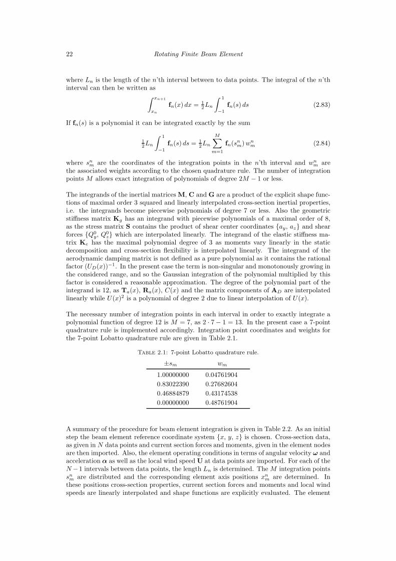
The necessary number of integration points in each interval in order to exactly integrate apolynomial function of degree 12 is M = 7, as 2 · 7− 1 = 13. In the present case a 7-pointquadrature rule is implemented accordingly. Integration point coordinates and weights forthe 7-point Lobatto quadrature rule are given in Table 2.1.
Table 2.1: 7-point Lobatto quadrature rule.
±sm wm
1.00000000 0.04761904
0.83022390 0.27682604
0.46884879 0.43174538
0.00000000 0.48761904
A summary of the procedure for beam element integration is given in Table 2.2. As an initialstep the beam element reference coordinate system {x, y, z} is chosen. Cross-section data,as given in N data points and current section forces and moments, given in the element nodesare then imported. Also, the element operating conditions in terms of angular velocity ω andacceleration α as well as the local wind speed U at data points are imported. For each of theN−1 intervals between data points, the length Ln is determined. The M integration pointssnm are distributed and the corresponding element axis positions xn
m are determined. Inthese positions cross-section properties, current section forces and moments and local windspeeds are linearly interpolated and shape functions are explicitly evaluated. The element

2.5 Modal Analysis for Stationary Rotation 23
integrands are then computed in the integration points by which the element matrices areintegrated according to (2.81) and (2.84). The mass matrix M and the elastic stiffnessmatrix Ke are independent of operating conditions and are therefore conveniently handledtogether in a computational environment. The geometric stiffness matrix depends on thecurrent internal stress field σ and is therefore computed individually. The apparent inertialterms G, G, C, fC and fG depend on the angular velocity ω and the angular acceleration α
and are therefore conveniently integrated collectively. The aerodynamic terms Da, Ka andfa are computed collectively, as these depend both on the angular velocity ω of the elementand the wind field U. When all element matrices and load vectors are integrated, these arecombined according to (2.77)-(2.79) to obtain the classical format (2.76).
Table 2.2: Beam element integration.
1) Define element reference coordinate system:
{x, y, z}2) Import cross-section data and nodal section forces and moments:
J, JE , {Qa, Ma, Qb, Mb}, a, h, C, β
3) Import operating conditions and wind speeds:
ω, α, U
4) Compute integration interval lengths and integration point coordinates:
Ln, xnm
5) Evaluate shape functions and cross-section data in integration points:
Nnm, N
′nm , Jn
,m, JnE,m, {Qn
m, Mnm}, anm, hn
m, Cnm, βn
m, Unm
6) Integrate constant element matrices:
M, Ke
7) Integrate geometric stiffness matrix:
Kg
8) Integrate apparent inertial matrices and force vectors:
G, G, C, fC , fG
9) Integrate aerodynamic matrices and force vector:
Da, Ka, fa
10) Combine element matrices and force vectors:
D = 2G−Da, K = Ke +Kg + G−C−Ka, f = fC − fG + fa
11) Equations of motion in classical format:
Mu+Du+Ku = f
2.5 Modal Analysis for Stationary Rotation
For stationary rotation with α = 0 and a non-turbulent wind field the system matricesof (2.76) are constant. If the effect of the constant centrifugal force is furthermore includedonly in terms of initial stresses corresponding to local equilibrium, the homogeneous partof (2.76) describes a linear system with natural eigenfrequencies and associated eigenvectors.In this section the adopted framework for modal analysis of the rotating system is presented.

24 Rotating Finite Beam Element
2.5.1 State-Space Formulation
A method for modal analysis of the conservative part of (2.76), i.e. without the aerodynamicterms is discussed in e.g. Geradin & Rixen [19]. The eigenvalue problem associated withthe homogeneous part of (2.76) in the original configuration-space is quadratic due to thepresence of the equivalent damping term D = 2G−Da. This implies that the eigenvectorsof the standard eigenvalue problem formulation (K + λM)u = 0 do not allow a modaldecoupling of the gyroscopic system. Such uncoupling is however possible when the equationsof motion (2.76) are written in the following state-space format,
[
M 00 K
] [
uu
]
+
[
D K−K 0
] [
uu
]
=
[
f0
]
(2.85)
which is a system of first order differential equations of twice the size of the original system.This format was introduced by Meirovitch [34] in his original solution of the associatedeigenvalue problem for conservative gyroscopic systems. By defining the state vector zT =[ uT , uT ] the problem can be written in the following compact form,
Az+Bz = F (2.86)
To formulate the eigenvalue problem associated with (2.86) it is now assumed that thesolution to the homogeneous part of (2.86) is of exponential form,
z = zjeλjt (2.87)
where z is a constant vector and λ is the inverse of a time constant. Inserting the solution(2.87) into (2.86) the following generalized eigenvalue problem is obtained,
(
B+ λjA)
zj = 0 (2.88)
where λj is the eigenvalue and zj the associated eigenvector. In the original solution ofthe eigenvalue problem for gyroscopic systems, Meirovitch [34] divided the problem into thesolution of two real-valued problems on standard form, for which the eigenvalues and associ-ated eigenvectors were also real-valued. In the present case the eigenvalue problem (2.88) issolved directly using standard numerical techniques and the resulting complex-valued modeshapes are interpreted directly as shown in the following section.
2.5.2 Eigensolution Analysis
The state-space eigenvectors zj include the classical eigenvectors uj , as they appear in theform
zTj = [λjuTj , u
Tj ] (2.89)
Thus, the physical modal vibration shape uj of a given mode is available from the state-spaceformat and is simply extracted as the upper or lower half of the eigenvector zj . Accordingto e.g. [19] the eigenvalues λj of the conservative part of the state-space eigenvalue problem(2.88), i.e. for Ka = 0 and Da = 0, can be written in the form
λj = −zTj Bzj
zTj Azj= −
2ixTj Byj
xTj Axj + yT
j Ayj(2.90)
where the third term is obtained by writing the state-space eigenvector in terms of its realand imaginary parts, zj = xj + iyj . In the case of conservative gyroscopic systems, i.e. forα = 0 and Ka = 0 the equivalent stiffness matrix K is symmetric and positive definite.Consequently, A is positive definite and symmetric. Furthermore, with Da = 0, B is skew-symmetric. As shown in e.g. [34, 19] this leads to purely imaginary eigenvalues appearing
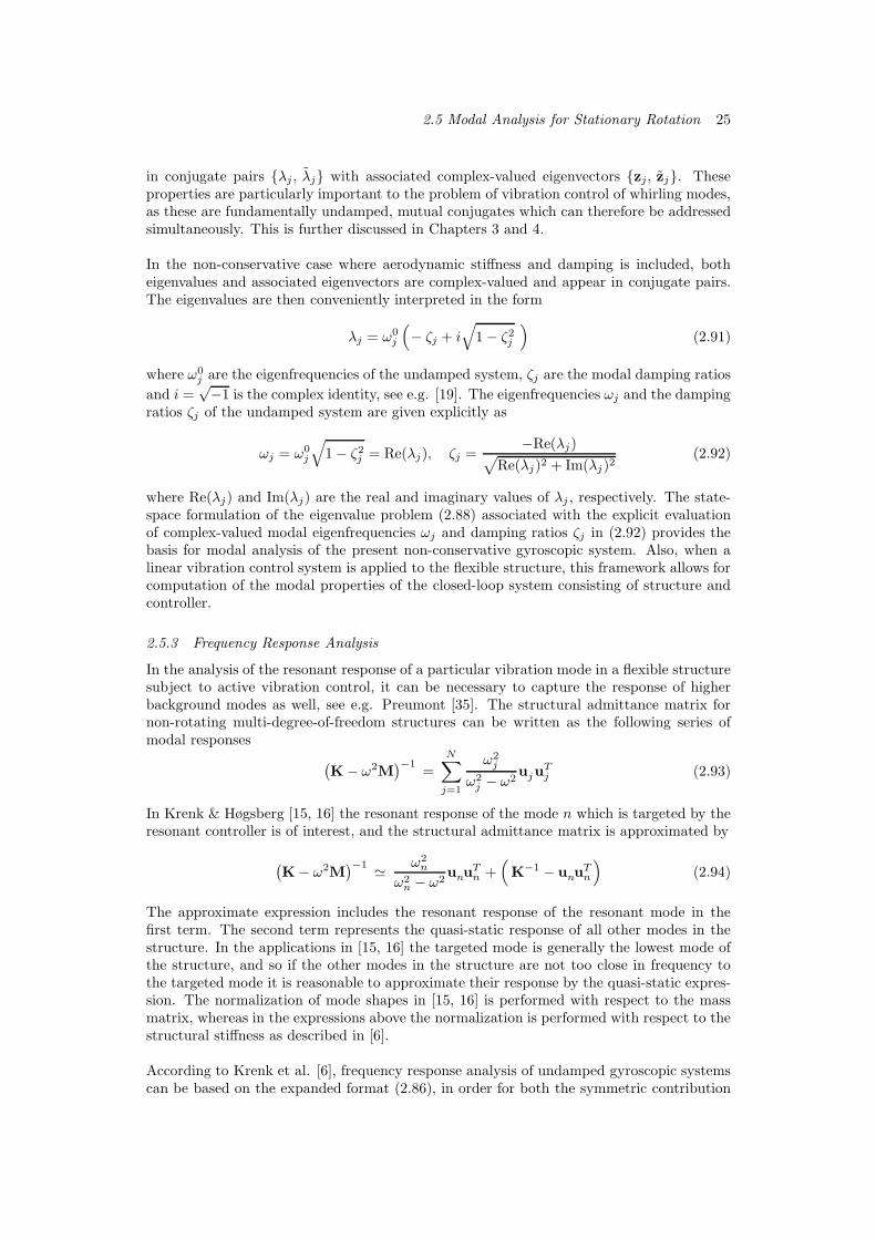
2.5 Modal Analysis for Stationary Rotation 25
in conjugate pairs {λj , λj} with associated complex-valued eigenvectors {zj, zj}. Theseproperties are particularly important to the problem of vibration control of whirling modes,as these are fundamentally undamped, mutual conjugates which can therefore be addressedsimultaneously. This is further discussed in Chapters 3 and 4.
In the non-conservative case where aerodynamic stiffness and damping is included, botheigenvalues and associated eigenvectors are complex-valued and appear in conjugate pairs.The eigenvalues are then conveniently interpreted in the form
λj = ω0j
(
− ζj + i√
1− ζ2j
)
(2.91)
where ω0j are the eigenfrequencies of the undamped system, ζj are the modal damping ratios
and i =√−1 is the complex identity, see e.g. [19]. The eigenfrequencies ωj and the damping
ratios ζj of the undamped system are given explicitly as
ωj = ω0j
√
1− ζ2j = Re(λj), ζj =−Re(λj)
√
Re(λj)2 + Im(λj)2(2.92)
where Re(λj) and Im(λj) are the real and imaginary values of λj , respectively. The state-space formulation of the eigenvalue problem (2.88) associated with the explicit evaluationof complex-valued modal eigenfrequencies ωj and damping ratios ζj in (2.92) provides thebasis for modal analysis of the present non-conservative gyroscopic system. Also, when alinear vibration control system is applied to the flexible structure, this framework allows forcomputation of the modal properties of the closed-loop system consisting of structure andcontroller.
2.5.3 Frequency Response Analysis
In the analysis of the resonant response of a particular vibration mode in a flexible structuresubject to active vibration control, it can be necessary to capture the response of higherbackground modes as well, see e.g. Preumont [35]. The structural admittance matrix fornon-rotating multi-degree-of-freedom structures can be written as the following series ofmodal responses
(
K− ω2M)
−1=
N∑
j=1
ω2j
ω2j − ω2
ujuTj (2.93)
In Krenk & Høgsberg [15, 16] the resonant response of the mode n which is targeted by theresonant controller is of interest, and the structural admittance matrix is approximated by
(
K− ω2M)
−1 ≃ ω2n
ω2n − ω2
unuTn +
(
K−1 − unuTn
)
(2.94)
The approximate expression includes the resonant response of the resonant mode in thefirst term. The second term represents the quasi-static response of all other modes in thestructure. In the applications in [15, 16] the targeted mode is generally the lowest mode ofthe structure, and so if the other modes in the structure are not too close in frequency tothe targeted mode it is reasonable to approximate their response by the quasi-static expres-sion. The normalization of mode shapes in [15, 16] is performed with respect to the massmatrix, whereas in the expressions above the normalization is performed with respect to thestructural stiffness as described in [6].
According to Krenk et al. [6], frequency response analysis of undamped gyroscopic systemscan be based on the expanded format (2.86), in order for both the symmetric contribution

26 Rotating Finite Beam Element
due to non-rotating effects and the skew-symmetric gyroscopic effects to be represented.This leads to the following form of the structural admittance matrix,
(
K+iω2G−ω2M)
−1=
N∑
j=1
[ ω2j
ω2j − ω2
12
(
uj uTj +uju
Tj
)
+ωωj
ω2j − ω2
12
(
uj uTj −uju
Tj
)
]
(2.95)
which is seen to be a 2N form of (2.93). The first term is real and symmetric and rep-resents the non-gyroscopic part of the response, while the second term is complex andskew-symmetric and represents the gyroscopic part of the response for rotating structuresrepresented in the rotating frame. To reach (2.95) the normalization
zTk A zTj = 2δkj , zTk B zTj = −2λj δkj (2.96)
is employed. The resonant response of mode n including a quasi-static approximation forthe higher modes is written in the form,
(K+ 2iωG− ω2M)−1 ≃ ω2n
ω2n − ω2
unuTn +
(
K−1 − 12
(
unuTn + unu
Tn
)
)
(2.97)
which is analogous to (2.94). It is seen that (2.94) is reproduced when the angular velocitybecomes zero and the eigenvectors become real-valued. The responses of the lower modes,1 ≤ j < n have been omitted in (2.97). This approximation is reasonable when these modeshave low participation uT
j f under the assumed harmonic loading of the system f . In [17]the expression (2.94) was used successfully despite the fact that the blade was rotating.The application was successful due to the fact that the MatLab programming environmentautomatically produces a Hermitian transpose of the complex-valued modes shapes, andthat the skew-symmetric contribution from gyroscopic forces is relatively small in the presentapplication.

Chapter 3
Rotor Systems in Finite Elements
The purpose of the present chapter is to present and illustrate the fundamental dynamicproperties of three-bladed rotors, both in general analytic form and in the particular case ofwind turbine rotors with blades of complex structural configuration and state-proportionalaerodynamics. As will be shown in Chapter 4, an analytic insight into and a good numericalreproduction of the three-bladed aeroelastic rotor system dynamics is essential for optimalsignal filtering and gain calibration of the resonant vibration control system. The presentchapter includes a series of numerical examples to illustrate selected properties of both iso-lated rotating blades and of full three-bladed rotors with realistic linearized properties ofthe structure, the aerodynamics and the operating conditions.
The finite element rotor model is assembled using a limited number of elements per blade andthe present chapter initially gives a simple procedure for coupling of the element equations.Local blade equations of motion are transformed into a common rotor coordinate systemfollowing the theory of consecutive finite rotations, see e.g. [27, 28]. Time integration ofthe rotor equations of motion is performed directly in the configuration-space format bythe classical Newmark procedure [36]. Rotor simulations are based on prescribed operatingconditions including e.g. angular rotor velocity and blade pitch angles. In each time stepoperation-dependent inertial and aerodynamic terms are updated explicitly and the non-linear geometric stiffness effects are subsequently established iteratively. An example ofan isolated rotating prismatic blade is given to introduce the direct complex mode shapeanalysis and to demonstrate how the model captures various geometric stiffness and inertialeffects in a transient analysis of a slightly modified reference blade, Maqueda et al. [37].An aeroelastic analysis of an isolated realistic 42m wind turbine blade under stationaryoperating conditions is performed and it is demonstrated that the finite element formulation[21, 17, 18] effectively models the blade with a limited number of elements. It is furthermoredemonstrated that the aerodynamic formulation produces a separation of strongly dampedflap-wise modes and weakly damped edge-wise modes. The modal dynamics of bladed rotorswith whirling effects is presented according to Krenk et al. [6] and the dynamics of whirlingare discussed in detail. An example based on an 86m wind turbine rotor is given whichillustrates the presence of the theoretical vibration phenomena in a realistic setting. Thegeneral description of three-bladed rotor dynamics and the numerical reproduction of thesefor the realistic aeroelastic 86m wind turbine rotor forms the basis for the development andvalidation of the resonant vibration control strategy presented in Chapter 4.
3.1 Rotor Assembly and Simulation
The full rotor is described in a rotating frame of reference {x, y, z}, in which the equationsof motion are defined. The rotor coordinate system rotates about the y-axis, by which theangular velocity of the rotor is ω = [ 0, ωy, 0 ]
T . The blades are discretized and assembledidentically, according to a default local coordinate system {x, y, z} in which the cross-sectionproperties are described. The local blade coordinate system is initially coinciding with therotor coordinate system, i.e. before the blade element matrices are rotated into positionin the rotor coordinate system. Prior to the assembly of the full rotor model, the system

28 Rotor Systems in Finite Elements
matrices of each blade are transformed into the rotor coordinate system according to theblade pitch angle βk, coning angle γk and azimuth angle θk where the index k representsthe blade number, i.e. k = 1, 2, 3. The pitch rotation axis nβ , the coning rotation axis nγ
and the azimuth rotation axis nθ are defined as
nβ = [ 1, 0, 0 ]T , nγ = [ 0, 0, 1 ]T , nθ = [ 0, 1, 0 ]T (3.1)
The pitch axis nβ initially coincides with the element reference axis, corresponding to actualblade pitch used in wind turbines for aerodynamic performance. In the present analysis theblades are assumed to have constant, identical pitch angles βk = βp. The coning rotation axisis seen to rotate the local blade coordinate system out of the rotor plane {x, z}. It i commonfor wind turbines to operate with a small, constant coning of each blade, i.e. γk = γc. This isto ensure tower clearance in the case of large out-of-plane blade deformations. The azimuthrotation axis positions the blades symmetrically with respect to the rotor axis y, e.g. with{θ1, θ2, θ3 } = {0, 2
3π,43π }.
3.1.1 Finite Element Rotor Model Assembly
The blades are assembled in the default local coordinate system, after which the equationsof motion for each blade are transformed according to the actual position and orientationof the blade in the rotor coordinate system. The rotor model is assembled by merging thethree blade root nodes in a common node, which defines the hub of the rotor. The rotor isconnected to the rotating frame by a flexible support of the hub, which is simply establishedvia a beam element which is coupled in one end to the rotor hub node and rigidly fixed inthe other end to the rotating coordinate system.
The relation between a coordinate vector designating a point in the local blade coordinatesystem xk and the corresponding vector in the rotor coordinate system x is defined as
x = Rkxk (3.2)
where Rk is the rotation matrix corresponding to the combined sequence of pitch rotationβk, coning rotation γk and azimuthal rotation θk in the mentioned order. As describedin Sec. 2.1 finite rotations are non-commuting, meaning that the sequence must chosencorrectly to obtain the desired combined rotation. The rotation matrix Rk is given as
Rk = Rkθ R
kγ R
kβ (3.3)
where the rotation matrices Rkβ, R
kγ and Rk
θ correspond to pure pitch, coning and azimuthalrotation respectively. The matrices are evaluated according to (2.6) and the sequential orderin (3.3) is defined as the reverse order of the combined rotation sequence, according to thetheory of consecutive finite rotations [27, 28].
Prior to the integration of inertial and aerodynamic blade element matrices, the local angularvelocity ωk and angular acceleration αk is determined according to the position of theelement in the rotor coordinate system, i.e. relative to the rotor angular velocity ω andangular acceleration α. The local blade angular velocities and accelerations are found bypre-multiplication with RT
k , e.g.ωk = RT
kω (3.4)
The aerodynamic element matrices and force vectors require the relative wind velocity Uk
in the local element coordinate system, for all data points defined along the element axis.This is obtained by the same inverse rotation of wind speeds defined in the rotor coordinatesystem U,
Uk = RTkU (3.5)

3.1 Rotor Assembly and Simulation 29
for blade k. The wind velocity vector U at the position x in the rotor coordinate system isevaluated as
U =
Ux(x)Uy(x)Uz(x)
− ω × x (3.6)
where the first term is obtained from a simulated or measured wind field and the secondterm represents the velocity of the undeformed structure.
When the blade elements are assembled in the local blade coordinate system the associateddegrees of freedom are denoted uk, the size of which depends on the number of nodes inthe discretization of the blades. The corresponding blade degrees of freedom in the rotorcoordinate system uk relate to the local blade degrees of freedom by the transformation
uk = Rkuk, Rk =
Rk
. . .
Rk
(3.7)
where the blade transformation matrix Rk consists of Rk as block-diagonal terms, corre-sponding in number to the number of nodes in blade k. The local blade matrices Mk, Dk,Kk and force vectors fk are similarly transformed into the corresponding matrices and forcevectors in the rotor coordinate system Mk, Dk, Kk and fk by the transformations
Mj = RkMkRTk , Dk = RkDkR
Tk , Kk = RkKkR
Tk , fk = Rk fk (3.8)
In order to obtain the equations of motion for the fully coupled rotor, the blade matricesMk, Dk, Kk and vectors fk are assembled in a single matrix form, where the root nodesof each blade are coupled in a common node, representing the hub of the rotor. A singlebeam element is used to provide a flexible shaft-like support of the rotor, through which theblades exchange root forces and moments. The element is perpendicular to the {x, z} rotorplane and is defined with cross-section properties corresponding to a solid, cylindrical shaftwith homogeneous material properties. One node is merged into the rotor hub node andthe degrees of freedom of the other node are assumed to be fixed to the origin of the rotorcoordinate system. This is the constraint that fixes the rotor to the rotating coordinatesystem and makes the structural system non-singular. The fixed degrees of freedom ofthe shaft element are conveniently eliminated from the equations of motion of the rotor.Correspondingly, the rotor model in the developed finite beam element formulation onlyhas nodes in the blades and the flexible rotor hub. The resulting equations of motion forthe rotor can then be written in the standard configuration-space format correspondingto (2.76),
Mu+Du+Ku = f (3.9)
where M is the rotor mass matrix, D is the equivalent rotor damping matrix, K is theequivalent rotor stiffness matrix and f is the rotor load vector, including both aerodynamicand inertial terms. The rotor assembly procedure is summarized in Table 3.1.
3.1.2 Integration of Rotor Equations of Motion
The rotor equations of motion (3.9) are simulated via the classical Newmark integrationalgorithm [36]. The algorithm establishes the system states {um+1, um+1} in time stepm + 1 based on known states {um, um} in time step m and known load vectors in theprevious and current time steps {fm, fm+1}. The algorithm is based on an approximateexpression of the displacement and velocity increments in terms of weighted values of the

30 Rotor Systems in Finite Elements
Table 3.1: Rotor assembly.
1) Define local blade reference axis:
{x, y, z}2) Global operating conditions:
θ, ω, α, U
3) Rotation matrices:
Rk, Rk
4) Compute local operating conditions:
ωk = RTkω, αk = RT
kα, Uk = RTkUk
5) Integrate local beam element matrices and load vectors:
M, D, K, f
6) Assemble blade matrices and load vectors in local reference axes:
Mk, Dk, Kk, fk
7) Rotate blade matrices and load vectors:
Mk = RkMkRTk , Dk = RkDkR
Tk , Kk = RkKkR
Tk , fk = Rk fk
8) Assemble global blade matrices and load vectors to obtain rotor model:
M, D, K, f
9) Equations of motion in classical format:
Mu+Du+Ku = f
accelerations in the previous and current acceleration states {um, um+1}, see e.g. [19, 28].The displacement and velocity increments can be written as
um+1 = um +
∫ tm+1
tm
u(τ) dτ
um+1 = um + hum +
∫ tm+1
tm
(tm+1 − τ)u(τ) dτ
(3.10)
where h is the time interval length, h = tm+1 − tm. The integrals are then evaluatedapproximately in terms of weighted interval end point values of the accelerations. Thisleads to the following approximate, but asymptotically correct expressions for small timeincrements,
um+1 = um + (1− γN)hum + γNhum+1
um+1 = um + hum + (12 − βN)h2um + βNh
2um+1
(3.11)
Here the parameters 0 < γN < 1 and 0 < βN < 12 are the forward weighting parameters,
where full weight on the previous acceleration states um corresponds to γN = 0 and βN = 0and full forward weighting corresponds to γN = 1 and βN = 1
2 . For linear systems the choiceof these parameters and the relative time step length max(ωj)h affects the stability, theaccuracy in system eigenfrequency reproductions and the numerical damping of the system.A commonly used setting is the so-called ‘average acceleration’ scheme with γN = 1
2 andγN = 1
4 , for which the integration algorithm is stable for any relative time step length. Bysatisfying the equations of motion at tm+1, the following equation for the current acceleration

3.2 Example: 8m Prismatic Rotor Blade 31
states um+1 is obtained,
(
M+ γhD+ βh2K)
um+1 = fm+1 −D(
um + (1− γN)hum
)
−K(
um + hum + (12 − βN)h2um
)
(3.12)
For linear systems a convenient procedure for computing the current states involves theintroduction of a set of prediction terms {u∗
m+1, u∗
m+1} in which the last terms in (3.11a)and (3.11b) are neglected. Equation (3.12) gives the current acceleration states um+1 andum+1 and um+1 are then found by providing the last terms in (3.11),
um+1 = u∗
m+1 + γNhum+1
um+1 = u∗
m+1 + βNh2um+1
(3.13)
The Newmark integration procedure as used in the present application is summarized inTable 3.2. In the present case the rotor equations of motion (3.9) are nonlinear due to thegeometric stiffness term which depends on the current stress state σm+1. Furthermore theapparent inertial terms are non-constant for non-constant angular velocity ω and angularaccelerationα of the rotor coordinate system, and the aerodynamic terms depend on currentangular velocity ω and the current wind velocity field. In the present case the apparent in-ertial and aerodynamic matrices and load vectors are updated explicitly in the current timestep, as these depend on prescribed operating conditions. When the equations of motion aresolved for the current time step according to equations 3.10-3.12, this is done in a simplefixed point iteration procedure where the current stress field σm+1 and consequently thegeometric element stiffness matrices Kg,m+1 is updated. For improved convergence speedthe previous stress field σm is used as an initial guess.
Nodal section forces and moments are evaluated on local element basis according to (2.80).The element matrices in the local blade coordinate system are readily available, and so thelocal element states {um+1, ˙um+1, ¨um+1} must be computed. This is done in a three-stepprocedure where the individual blade state vectors with respect to the rotor system are firstextracted and then transformed into the local blade coordinate system by pre-multiplicationwith RT
k . The local element states are finally extracted from the local blade state vectors.The procedure is shown in Table 3.2, in the steps 9a)-c).
3.2 Example: 8m Prismatic Rotor Blade
The present finite beam element formulation is developed in order to capture the mostimportant inertial and stiffness effects for rotating beams with small deformation-inducedcross-section displacements and rotations. The formulation is linear for stationary operatingconditions and non-linear under transient conditions. In the stationary case, modal analysiscan be performed to obtain the information on the dynamic properties of the structurewhich is essential to controller calibration, and for investigation of transient performance thenon-linear equations of motion can be integrated by the integration scheme summarized inTable 3.2. This section is devoted to an example which demonstrates how the model capturesgeometric and centrifugal stiffness effects, gyroscopic forces and the centrifugal and angularacceleration loads. A simple rotating beam with a small mass center offset is analyzedin terms of modal properties under different stationary angular velocities. Subsequently,the beam is subjected to a spin-up maneuver for transient response analysis. The bladegeometry and operating conditions are inspired by Maqueda et al. [37].

32 Rotor Systems in Finite Elements
Table 3.2: Integration of rotor equations of motion.
1) Initial conditions:
u0, u0
2) Time increment:
tm+1 = tm + h
3) Import global current operating conditions:
θm+1, ωm+1, αm+1, Um+1
4) Compute local current operating conditions:
ωm+1,k = RTkωm+1, αm+1,k = RT
kαm+1, Um+1,k = RTkUm+1
5) Approximate internal section forces and moments:
[−QTa , −MT
a , QTb , M
Tb ]Tm+1 = [−QT
a , −MTa , Q
Tb , M
Tb ]Tm
6) Assemble rotor:
a) Local element matrices and load vectors:
M, Dm+1, Km+1, fm+1
b) Global rotor matrices and load vectors:
M, Dm+1, Km+1, fm+1
7) Prediction step:
u∗
m+1 = um + (1 − γ)hum
u∗
m+1 = um + hum + (1
2− β)h2um
8) Correction step:
M∗ = M+ γhDm+1 + βh2Km+1
um+1 = M−1∗
(
fm+1 −Dm+1u∗
m −Km+1u∗
m+1
)
um+1 = u∗
m+1 + γhum+1
um+1 = u∗
m+1 + βh2um+1
9) Section forces:
a) Extract global blade states:
um+1,k, um+1,k, um+1,k
b) Rotate to local blade coordinate systems:
um+1,k = RTk um+1,k, ˙um+1,k = RT
k um+1,k, ¨um+1,k = RTk um+1,k
c) Extract local element states:
um+1, ˙um+1, ¨um+1
d) Compute local element section forces and moments:
[−QTa , −MT
a , QTb , M
Tb ]Tm+1 =
M ¨um+1 + Dm+1˙um+1 + Km+1um+1 − fm+1
10) For improved accuracy on geometric stiffness re-run 6)-9).
11) Return to 2) or stop.

3.2 Example: 8m Prismatic Rotor Blade 33
3.2.1 The Rotor Blade
The beam is shown in Fig. 3.1, and it consists of two prismatic parts. The primary partis a narrow rectangular cross-section profile, which provides the main stiffness of the beam.The secondary part is small compared to the primary part and it therefore has vanishingcontribution to the overall stiffness of the beam.
x
yz
ω
Figure 3.1: Cantilever beam with mass center offset.
One end of the beam is fixed at the origin of the rotating reference frame, i.e. q(0) = 0 andr(0) = 0, while the other end is free. The width and height of the primary cross-section partis wb = 0.035m and hb = 0.35m, and it is located such that the longitudinal line of symmetrycoincides with reference axis x, while the cross section axes of symmetry are parallel to they- and z-axis. The material is homogeneous and isotropic with mass density = 2700kg/m3,modulus of elasticity E = 72GPa and Poisson ratio ν = 0.35. The symmetric distributionof the homogeneous and isotropic material with respect to the y- and z-axis implies thatthe shear center and the elastic center coincide at the reference axis. The elastic and shearprincipal axes are furthermore parallel to the y- and z-axis.
The secondary part with the quadratic cross-section has width and height wb and it is lo-cated adjacent to the main section, with its center of symmetry intersecting the y-axis. Thematerial is homogeneous with mass density = 7850kg/m3. The presence of this secondarypart implies that the mass center G of the entire cross-section has coordinates gy ≃ − 1
4wb
and gz = 0, thus introducing a slight mass offset from the reference axis.
Inertial and axial elastic cross-section properties are determined according to the expressionsin (2.16) and (2.29). Since the principal bending and shear axes are parallel to the y- and z-axis, no off-diagonal terms arise in the cross-section stiffness matrix Dc. The shear stiffnesscomponents AG
yy and AGzz are set to GA0, where G = 1
2E/(1 + ν) is the shear modulus and
A0 = 56wh is the cross-section shear area, accounting for a non-uniform distribution of the
shear stresses in the rectangular cross-section. The torsional stiffness is approximated byKG = 1
3Ghw3. This holds for narrow cross-sections, i.e. wb ≪ hb, where the contributionfrom shear stresses σxz to the torsional moment Mx can be neglected.
3.2.2 Modal Analysis
The present beam is rotated about the y-axis, i.e. ω = [ 0, ωy, 0 ]T , and modeled using 8
elements of identical length. Solutions to the eigenvalue problem (2.88) are computed atstationary states α = 0 where the geometric stiffness matrix Kg is established accordingto the stress state from constant centrifugal forces fC with 4 fixed point iterations on theinternal stresses. The stress integral S0 is approximated by S0 ≃ r2AQ
0x, where the radius of
gyration with respect to the shear center is evaluated as r2A = (Iyy + Izz)/(wbhb).
The first three eigenfrequencies are plotted as function of the rotational frequency in Fig. 3.2.The values are normalized with respect to the fundamental eigenfrequency at zero rotationalvelocity ω0
1 . The first two modes are the first and second bending modes in the y-direction

34 Rotor Systems in Finite Elements
and the associated eigenfrequencies are seen to increase due to stiffening from the positivedefinite geometric stiffness contribution. The third mode is the first bending mode in thez-direction. This mode vibrates in the rotor plane whereby the negative definite centrifugalstiffness contribution is activated and counteracts the geometric stiffening. The eigenfre-quency ω3 hereby increases at a significantly slower rate than ω1 and ω2. In Krenk et al. [6]an approximate, explicit expression for the change of eigenfrequency with rotation speed isgiven, based on a perturbation analysis of the quadratic eigenvalue problem of size N asso-ciated with the equations of motion (2.76). Predicted values are shown by cross markers ×and the analytical expression is seen to match the frequency developments very well.
0 1 2 3 4 5 6 7 8 9 100
2
4
6
8
10
12
ωy [rad/s]
ωn/ω
0 1
ω1/ω0
1
ω2/ω0
1
ω3/ω0
1
Figure 3.2: Structural eigenfrequencies ωn/ω1 as function of angular velocity ωy.
The complex-valued mode shape u3 for ωy = 7rad/s is shown in Fig. 3.3, where the realand imaginary values of the nodal displacements qx, qy, qz and the torsional rotations rxare plotted at the element nodes. The natural eigenfrequency is ω3 = 23.76rad/s. Thenormalization of the modes is chosen such that the largest value of qz is purely imaginaryand has the amplitude -1. The classic fundamental mode shape of a cantilever beam isrecognized in Fig. 3.3a. The mass center G has an offset from the shear center A in they-direction. This implies that for any vibration modes with a displacement component inthe z-direction, this displacement will couple to torsion rx. This is seen in Fig. 3.3b, wherethe torsional component rx is shown. The scaling of the mode implies that the velocityqz of the beam tip is purely real with a positive real part. The fact that the blade istraveling with a finite, positive in-plane velocity at the chosen phase in the modal oscillationmeans that gyroscopic forces, proportional to the velocity, are invoking compressive axialdeformations of the beam, qx < 0. These are shown in Fig. 3.3c, and the −π/2 phase lagto the displacement components is seen in terms of the purely real axial deformations qx.The resulting component of the axial gyroscopic force-intensity of a cross-section is locatedin the mass center G of the cross-section. As the mass center has an offset in the y-directionfrom the elastic center C, bending moments about the z-axis are induced. This results intransverse displacements qy, as shown in Fig. 3.3d. The deflection shape is almost identicalto that of mode 2, as modes 2 and 3 have closely spaced eigenfrequencies at the currentangular velocity.
3.2.3 Spin-Up Maneuver
The beam is subjected to a spin-up maneuver with a prescribed development of the rotationabout the y-axis θy(t) given as
θy(t) =
{
13ωy t
3/t21 for 0 ≤ t ≤ t1
ωy(t− 23 t1) for t > t1
(3.14)
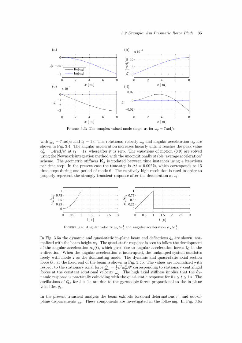
3.2 Example: 8m Prismatic Rotor Blade 35
0 2 4 6 8
−1
−0.5
0
Re(u3)Im(u3)
0 2 4 6 8
0
5
10
x 10−4
0 2 4 6 8
−3
−2
−1
0
x 10−4
0 2 4 6 8
−0.02
0
0.02
x [m ]x [m ]
x [m ]x [m ]
q z
r x[rad/m
]
q x q y
(a) (b)
(c) (d)
Figure 3.3: The complex-valued mode shape u3 for ωy = 7rad/s.
with ωy = 7 rad/s and t1 = 1 s. The rotational velocity ωy and angular acceleration αy areshown in Fig. 3.4. The angular acceleration increases linearly until it reaches the peak valueα1y = 14rad/s2 at t1 = 1s, whereafter it is zero. The equations of motion (3.9) are solved
using the Newmark integration method with the unconditionally stable ‘average acceleration’scheme. The geometric stiffness Kg is updated between time instances using 4 iterationsper time step. In the present case the time-step is ∆t = 0.0027s, which corresponds to 15time steps during one period of mode 6. The relatively high resolution is used in order toproperly represent the strongly transient response after the deceleration at t1.
0 0.5 1 1.5 2 2.5 3
00.250.5
0.751
0 0.5 1 1.5 2 2.5 3
00.250.5
0.751
t [ s ]t [ s ]
ωy/ω
y
αy/αy
Figure 3.4: Angular velocity ωy/ω1
y and angular acceleration αy/α1
y .
In Fig. 3.5a the dynamic and quasi-static in-plane beam end deflections qz are shown, nor-malized with the beam height wb. The quasi-static response is seen to follow the developmentof the angular acceleration αy(t), which gives rise to angular acceleration forces fG in thez-direction. When the angular acceleration is interrupted, the undamped system oscillatesfreely with mode 2 as the dominating mode. The dynamic and quasi-static axial sectionforce Qx at the fixed end of the beam is shown in Fig. 3.5b. The values are normalized withrespect to the stationary axial force Q
x= 1
2L2ω2
yA corresponding to stationary centrifugal
forces at the constant rotational velocity ωy. The high axial stiffness implies that the dy-namic response is practically coinciding with the quasi-static response for 0 s ≤ t ≤ 1 s. Theoscillations of Qx for t > 1 s are due to the gyroscopic forces proportional to the in-planevelocities qz.
In the present transient analysis the beam exhibits torsional deformations rx and out-of-plane displacements qy. These components are investigated in the following. In Fig. 3.6a

36 Rotor Systems in Finite Elements
0 0.5 1 1.5 2 2.5 3
−0.5
−0.25
0
0.25
0.5
0 0.5 1 1.5 2 2.5 3
0
0.25
0.5
0.75
1
1.25
t [ s ]t [ s ]
q z/hb
Qx/Q
x
Figure 3.5: Dynamic and quasi-static responses. a) Free end displacements qz. b)Fixed end axial force Qx.
the torsional root moment Mx is shown, normalized with respect to the moment generatedby the angular acceleration forces at αy, which is given as Mx = 1
2L2Agyαy. As the mag-
nitude of αy increases, angular acceleration forces are introduced.
During the first approximately 0.7 s this results in a negative (clockwise) torsional rotationrx, with a corresponding negative moment Mx. Simultaneously, during the first 0.7 s, apositive shear force Qz and a negative moment My appear due to the positive transversedisplacements qz. Corresponding changes in geometric stiffness arise in terms of the torsion-displacement derivative coupling (rx, q
′
y) due to Qz and in terms of the torsion derivative-rotation derivative coupling (r′x, r
′
z) due to My. These coupling effects have opposite direc-tion, where the torsion-displacement coupling by Qz is dominant in the present case. Thus,the negative rotation rx invokes positive displacements qy.
After approximately 0.7 s the centrifugal forces fC evolve significantly, and the resultingcentrifugal force has both an axial component Qx and a transverse component Qy, actingin the mass center. The transverse component demands negative displacements qy, whileQx has the opposite effect via the resulting bending moment about the z-axis. Here thelatter component dominates and positive displacements qy appear as shown in Fig. 3.6b.The torsion-displacement derivative coupling (rx, q
′
y) due to Qz implies that positive dis-placements qy will induce a negative (clockwise) torsional rotation of the beam. This effecthas opposite sign compared to the torsion induced by the angular acceleration forces andit is seen in Fig. 3.6a that the torsional root moment Mx starts to increase when the dis-placements qy become significant due to the presence of centrifugal forces. The significantvibrations qy for t < 1 are a combination of modes 1, 2 and 3 where mode 3 contributes dueto the presence of non-working gyroscopic forces.
The modal analysis of the prismatic rotating beam shown in the present example has demon-strated in a simple way how direct analysis of complex-valued mode shapes provides a com-plete description of the modal dynamics of a rotating beam. It is furthermore demonstratedthat the model captures tractable geometric and centrifugal stiffness effects, gyroscopic forcesand the centrifugal and angular acceleration loads in a transient analysis. In the followingsection the element formulation is used to analyze the dynamics of a realistic wind turbineblade.
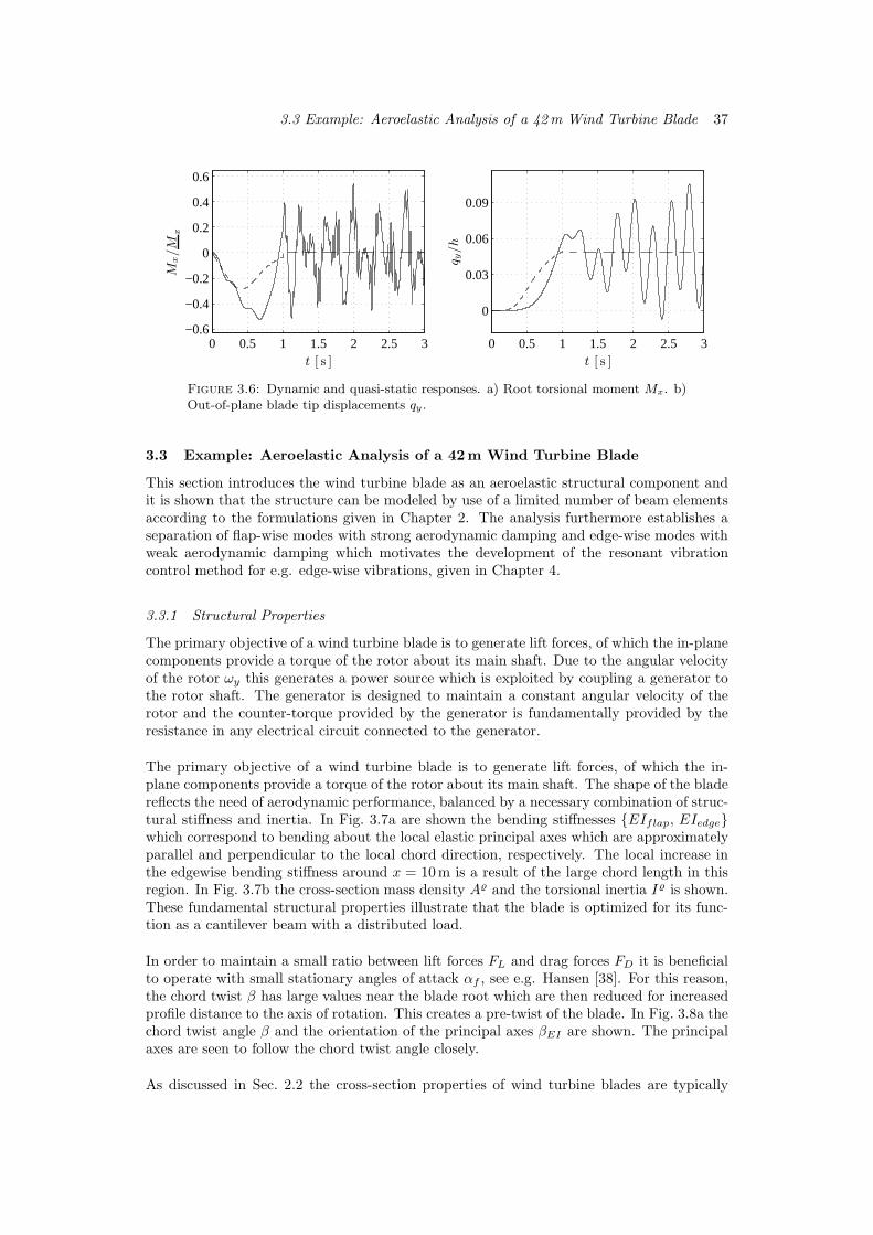
3.3 Example: Aeroelastic Analysis of a 42m Wind Turbine Blade 37
0 0.5 1 1.5 2 2.5 3−0.6
−0.4
−0.2
0
0.2
0.4
0.6
0 0.5 1 1.5 2 2.5 3
0
0.03
0.06
0.09
t [ s ]t [ s ]
Mx/M
x
q y/h
Figure 3.6: Dynamic and quasi-static responses. a) Root torsional moment Mx. b)Out-of-plane blade tip displacements qy .
3.3 Example: Aeroelastic Analysis of a 42m Wind Turbine Blade
This section introduces the wind turbine blade as an aeroelastic structural component andit is shown that the structure can be modeled by use of a limited number of beam elementsaccording to the formulations given in Chapter 2. The analysis furthermore establishes aseparation of flap-wise modes with strong aerodynamic damping and edge-wise modes withweak aerodynamic damping which motivates the development of the resonant vibrationcontrol method for e.g. edge-wise vibrations, given in Chapter 4.
3.3.1 Structural Properties
The primary objective of a wind turbine blade is to generate lift forces, of which the in-planecomponents provide a torque of the rotor about its main shaft. Due to the angular velocityof the rotor ωy this generates a power source which is exploited by coupling a generator tothe rotor shaft. The generator is designed to maintain a constant angular velocity of therotor and the counter-torque provided by the generator is fundamentally provided by theresistance in any electrical circuit connected to the generator.
The primary objective of a wind turbine blade is to generate lift forces, of which the in-plane components provide a torque of the rotor about its main shaft. The shape of the bladereflects the need of aerodynamic performance, balanced by a necessary combination of struc-tural stiffness and inertia. In Fig. 3.7a are shown the bending stiffnesses {EIflap, EIedge}which correspond to bending about the local elastic principal axes which are approximatelyparallel and perpendicular to the local chord direction, respectively. The local increase inthe edgewise bending stiffness around x = 10m is a result of the large chord length in thisregion. In Fig. 3.7b the cross-section mass density A and the torsional inertia I is shown.These fundamental structural properties illustrate that the blade is optimized for its func-tion as a cantilever beam with a distributed load.
In order to maintain a small ratio between lift forces FL and drag forces FD it is beneficialto operate with small stationary angles of attack αf , see e.g. Hansen [38]. For this reason,the chord twist β has large values near the blade root which are then reduced for increasedprofile distance to the axis of rotation. This creates a pre-twist of the blade. In Fig. 3.8a thechord twist angle β and the orientation of the principal axes βEI are shown. The principalaxes are seen to follow the chord twist angle closely.
As discussed in Sec. 2.2 the cross-section properties of wind turbine blades are typically

38 Rotor Systems in Finite Elements
0 10 20 30 40
0
0.2
0.4
0.6
0.8
1
1.2
EIflap/EI0
flap
EIedge/EI0
edge
0 10 20 30 40
0
0.2
0.4
0.6
0.8
1
A/A
0
I/I0
x [m ]x [m ]
Figure 3.7: Principal flap/edge bending stiffnesses EI and inertial parameters A
and I.
of general character due to e.g. the non-trivial geometry and non-homogeneous materialcomposition. In Fig. 3.8b is shown the distances from the blade reference axis of the masscenter g′z, the elastic center c′z and the shear center a′z . The distances are measured alongthe chord and are positive towards the trailing edge. The values are normalized by the rootchord C0. The positions of these characteristic centers are seen to vary significantly over thelength of the blade. The local discontinuities of the shear center positions are due to localchanges in the shear web configuration.
0 10 20 30 40
0
0.2
0.4
0.6
0.8
1
β/β0
βEI/β0
0 10 20 30 40
−0.1
−0.05
0
0.05
0.1
0.15
0.2
0.25
c′z/C0
a′
z/C0
g′z/C0
x [m ]x [m ]
Figure 3.8: Chord angle β, principal axes angle βc and z-coordinates of characteristiccenters.
Typically wind turbines are operated at constant angular velocity within a given rangeof atmospheric mean wind speeds. In this range the power output of the turbine is keptconstant, and in order to maintain a constant aerodynamic torque on the rotor, the bladesare rotated about their longitudinal reference axes by an active pitch system. In Fig. 3.9an example of an operating region is shown. The figure shows the stationary rotor angularvelocity ωy and active pitch angle βp as function of mean wind speed Uy. The shown regimeis a variant of that used by Østergaard et al. [39]. It is seen that the operating regimeinvolves significant variations in rotor angular velocity and blade pitch angles.
The significant changes in blade cross-section parameters throughout the blade length impliesthat the blade is modelled effectively with a finite element formulation that accounts fornon-constant cross-section properties, internal stresses and aerodynamic forces. In the nextsection a static analysis of a single wind turbine blade is performed and modeling convergenceis investigated.

3.3 Example: Aeroelastic Analysis of a 42m Wind Turbine Blade 39
0 4 8 12 16 20 24 288
10
12
14
16
0 4 8 12 16 20 24 28
0
10
20
30
Uy [m/s ]Uy [m/s ]
ωy[rpm
]
βp[d
eg.]
Figure 3.9: Rotational velocity ω and pitch angle as function of wind speed Uy .
3.3.2 Static Analysis
The wind turbine blade is in the case of stationary operation loaded by constant centrifugaland aerodynamic forces. The aerodynamic lift and drag forces depend on the angular velocityof the rotor ω, the mean wind speed Uy and the resulting inflow angles due to the blade pitch
angle βp and the chord twist angles β(x). In Fig. 3.10a the resulting inflow speeds U(x)are shown for stationary operation at 12m/s and 20m/s and in Fig. 3.10b the resultinginflow angles αU(x) − β(x) are shown. In both figures the values are normalized withrespect to the root values. The inflow angles are within the region of ±10 degrees forapproximately x > 1
3L, where L is the blade length. In this region it is reasonable fortypical aerodynamic profiles to assume that the flow around the profile is laminar, whichimplies that the stationary aerodynamic lift is proportional to the inflow angle. For anincompressible fluid the lift coefficient can be shown to be CL = 2π for thin aerodynamicprofiles, and conventional profiles have been shown experimentally to come close to thisvalue [23]. Fig. 3.10 hereby demonstrates that the stationary lift formulation in Sec. 2.3 isreasonable for the present application.
0 5 10 15 20 25 30 35 400
1
2
3
4
5
6
Uy = 12 m/s
Uy = 20 m/s
0 5 10 15 20 25 30 35 40
0
0.2
0.4
0.6
0.8
1
Uy = 12 m/s
Uy = 20 m/s
x [m ]x [m ]
U/U
0
(αU−
β)/(α
0 U−
β0)
Figure 3.10: Local inflow velocity U and inflow angle αU − β.
The stationary structural response for the 42m blade operating at the mean wind speedUy = 12m/s is shown in Fig. 3.11 in terms of nodal displacements qy and qz extractedfrom the rotor displacement vector u which is defined in the rotor coordinate system. Thevalues are normalized with respect to the maximum blade tip deflection, qLy . The blade isrotating with ωy = 1.57 rad/s corresponding to 15 rpm, and it has the coning angle γ1 = −6o
and the pitch angle β1 = 4.4o, corresponding to Svendsen et al. [18]. The lift center D isassumed to be located on the chord, one quarter of the chord length from the leading edgeof the profile. The aerodynamic lift component FL gives rise to significant out-of planedisplacements qy and somewhat smaller in-plane deflections qz , as seen in Fig. 3.11a and b.The in-plane deflections qz represent the part of the aerodynamic lift which generates rotor
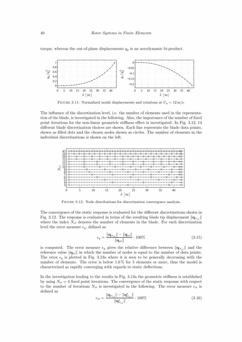
40 Rotor Systems in Finite Elements
torque, whereas the out-of-plane displacements qy is an aerodynamic bi-product.
0 5 10 15 20 25 30 35 40
0
0.2
0.4
0.6
0.8
1
0 5 10 15 20 25 30 35 40
−0.2
−0.15
−0.1
−0.05
0
x [ m ]x [ m ]
q y/qL y
q z/qL y
Figure 3.11: Normalized nodal displacements and rotations at Uy = 12m/s.
The influence of the discretization level, i.e. the number of elements used in the representa-tion of the blade, is investigated in the following. Also, the importance of the number of fixedpoint iterations for the non-linear geometric stiffness effect is investigated. In Fig. 3.12, 14different blade discretization choices are shown. Each line represents the blade data points,shown as filled dots and the chosen nodes shown as circles. The number of elements in theindividual discretizations is shown on the left.
0 5 10 15 20 25 30 35 40
3456789
10111215202445
x [m ]
Nel
Figure 3.12: Node distributions for discretization convergence analysis.
The convergence of the static response is evaluated for the different discretizations shown inFig. 3.12. The response is evaluated in terms of the resulting blade tip displacement ‖qNel
‖where the index Nel denotes the number of elements in the blade. For each discretizationlevel the error measure ǫq, defined as
ǫq =‖qNel
‖ − ‖q45‖‖q45‖
· 100% (3.15)
is computed. The error measure ǫq gives the relative difference between ‖qNel‖ and the
reference value ‖q45‖ in which the number of nodes is equal to the number of data points.The error ǫq is plotted in Fig. 3.13a where it is seen to be generally decreasing with thenumber of elements. The error is below 1.0% for 5 elements or more, thus the model ischaracterized as rapidly converging with regards to static deflections.
In the investigation leading to the results in Fig. 3.13a the geometric stiffness is establishedby using Nit = 4 fixed point iterations. The convergence of the static response with respectto the number of iterations Nit is investigated in the following. The error measure ǫit isdefined as
ǫit =‖qNel
‖ − ‖q8
Nel‖
‖q8
Nel‖ · 100% (3.16)

3.3 Example: Aeroelastic Analysis of a 42m Wind Turbine Blade 41
where the reference value ‖q8
Nel‖ corresponds to the resulting blade tip displacement for
a blade modeled with Nel elements and the geometric stiffness is established in Nit = 8iterations. The development of the error ǫit is shown in Fig. 3.13b for Nel = {4, 8, 15, 45}elements. The error is seen to be monotonously decreasing and the deviation from thereference value is in all cases below 0.1% for Nit = 3 or more. The monotonous decrease inthe error demonstrates that the formulation for the geometric stiffness via initial stresses isrobust and rapidly converging in the present application.
1 2 3 4 5 6 7
10−9
10−7
10−5
10−3
10−1
101
Nel = 4Nel = 8Nel = 15Nel = 45
5 10 15 20 2510
−2
10−1
100
101
Nit
ǫ it[%
]
Nel
ǫ q[%
]
Figure 3.13: a) Displacement convergence with discretization level. b) Displacementconvergence with geometric stiffness iterations.
The results in the present section demonstrate that the element formulation is robust andrapidly converging in terms of discretization and fixed point iteration of the geometric stiff-ness. The investigations have so far only considered the stationary static response. In thefollowing section the performance of the model is investigated in the case of modal analysis.
3.3.3 Modal Analysis
When the eigenvalue problem (2.88) is solved the solution quality can be evaluated by thedimensionless error measure ǫuj
, defined as
ǫuj=
‖ (K+ λjD+ λ2jM )uj ‖
‖Kuj ‖(3.17)
where index j denotes the eigensolution number. The numerator should be equal to zero,however this is rarely fulfilled by the numerical solution of the eigenvalue problem. InFig. 3.14 the error measures for the first four eigensolutions {ǫu1
, ǫu2, ǫu3
, ǫu4} are plotted
as function of the number of elements in the model Nel. The eigenvalue problem is solvedwith the built-in solver eig of the commercial programming environment Matlabr, versionR2010a. The error is seen to generally increase with the number of elements, i.e. the solutionquality is reduced with the size of the problem (2.88). The solution quality is consideredacceptable in the entire region. For simpler systems the error is in the author’s experiencehowever typically smaller than 10−9.
Within the limits of the numerical solution of the eigenvalue problem, the solution of theeigenfrequencies ωj and damping ratios ζj should converge with increasing discretizationlevel. This is investigated by the eigenfrequency error measure ǫω and the damping ratioerror measure ǫζ , defined as
ǫωj=
‖ωj − ω25j ‖
ω25j
· 100%, ǫζj =‖ ζj − ζ25j ‖
‖ ζ25j ‖ · 100% (3.18)

42 Rotor Systems in Finite Elements
5 10 15 20 2510
−12
10−10
10−8
10−6
ǫu1
ǫu2
ǫu3
ǫu4
Nel
ǫ uj
Figure 3.14: Eigensolution error ǫujfor modes 1-4.
where ω25j and ζ25j are the reference values for a discretization of the blade with 25 elements.
The eigenfrequency error measures for the first four modes {ǫ1, ǫ2, ǫ3, ǫ4} are plotted inFig. 3.15a. The errors are seen to exhibit an overall decrease with Nel for approximatelyNel ≤ 10, and for Nel = 5 elements or more, the eigenfrequency errors are below 1.0%, whichmust be characterized as a rapid convergence. The damping ratio error measures are plottedin Fig. 3.15b and the convergence of these values is seen to be less pronounced. It is howeverclear that the errors {ǫζ1 , ǫζ2} of the two first modes are below 5% which is considereda satisfactory result for the present purpose. It has not been clarified why the dampingratios have a less pronounced convergence than the eigenfrequencies. The eigenfrequenciesrepresent the balance between modal stiffness and mass, whereas the damping ratios arisefrom the aerodynamic formulation. Thus, the explanation is probably to be found in theaerodynamic formulation.
5 10 15 2010
−3
10−2
10−1
100
101
102
ǫω1
ǫω2
ǫω3
ǫω4
5 10 15 2010
−3
10−2
10−1
100
101
102
ǫζ1
ǫζ2
ǫζ3
ǫζ4
NelNel
ǫ ωj[%
]
ǫ ζj[%
]
Figure 3.15: Eigenfrequency and damping convergence error for modes 1-4.
In the following the first two vibration modes of an isolated 42m blade are presented for thestationary operating conditions corresponding to a mean wind Uy = 12m/s and an angularvelocity of 15 rpm as introduced in the previous section. The first blade vibration mode u1
is termed the first ‘flap-wise’ mode, and it is dominated by bending about the weak axis ofthe blade, corresponding to dominant local displacements qy. This type of mode is stronglydamped due to the significant modal velocities ˙qz generated in the rear aerodynamic centerH , see e.g. (2.48). The mode has the eigenfrequency ω1 = 6.150 rad/s and the relativelyhigh damping ratio ζ1 = 0.418.
The second vibration mode of the blade u2 is termed the first ‘edge-wise’ mode, as it is dom-

3.3 Example: Aeroelastic Analysis of a 42m Wind Turbine Blade 43
inated by bending about the strong axis of the blade, corresponding to local displacementsqz. Vibrations in the edge-wise direction only have small influence on the relative inflowangle, and so this type of mode typically has weak aerodynamic damping. The mode hasthe eigenfrequency ω2 = 9.161 rad/s and the damping ratio ζ2 = 0.007, which is recognizedas a relatively low value, as expected. This result corresponds qualitatively to experimen-tal and theoretical results for pitch-regulated wind turbines of comparable size, [2, 3]. Inpractice the damping ratio will be somewhat higher than predicted here due to the presenceof intrinsic structural damping and non-linear aerodynamic effects which are not represented.
The mode shape u2 corresponding to the local blade coordinate system is shown in Fig. 3.16,in which the mode shape is scaled by phase and amplitude such that the local edge-wise bladetip displacement qz is purely real with unit amplitude. The real and imaginary values of qzare plotted in Fig. 3.16a and the typical vibration mode of a cantilever beam is immediatelyrecognized. The flap-wise displacements qy are shown in Fig. 3.16b where significant real andimaginary components are present. In the present scaling of the mode shape the imaginarypart represents a part of the flapwise displacements which have a π/2 phase differenceto the edge-wise displacements. This implies that when the blade oscillates in mode 2,the cross-sections follow elliptical trajectories in the local cross-section plane {y, z}. Thiselliptical motion is caused by the linear, velocity-proportional aerodynamic forces which areperforming a finite amount work on the blade. For the present mode the work is dissipative,corresponding to damping of the system. For completeness the torsional components rx areplotted in Fig. 3.16c and the axial components qx are plotted in Fig. 3.16d. The blade isseen to exhibit relatively small couplings to these components in edge-wise vibration andthe axial compression measured in the reference axis is dominated by the bending-induceddisplacements due to the offset of the elastic center from the blade reference axis.
0 5 10 15 20 25 30 35 400
0.25
0.5
0.75
1
Re(u2)Im(u2)
0 5 10 15 20 25 30 35 400
0.2
0.4
0 5 10 15 20 25 30 35 40
−0.06
−0.04
−0.02
0
0 5 10 15 20 25 30 35 40
00.5
11.5
2x 10
−3
x [ m ]
x [ m ]x [ m ]
q z q y
r x[rad/m
]
q x
(a) (b)
(c) (d)
Figure 3.16: The edgewise vibration mode u2 in local coordinates for Uy = 12m/s.
As shown in Fig. 3.9 the turbine rotor is subjected to signification changes in operationconditions within a typical operation regime. This will affect the modal properties of theblades. In Fig. 3.17a the development of the first two blade eigenfrequencies is shownaccording to the operation points in Fig. 3.9. The values are normalized with respect tothe eigenfrequencies in the initial point of operation with Uy = 4m/s. The first mode isseen to exhibit an increase in eigenfrequency of more than 10%. This is primarily due tothe fact that the mode is dominated by out-of-rotor-plane displacement components qz forwhich the geometric stiffening is not counteracted by centrifugal softening. The fact that
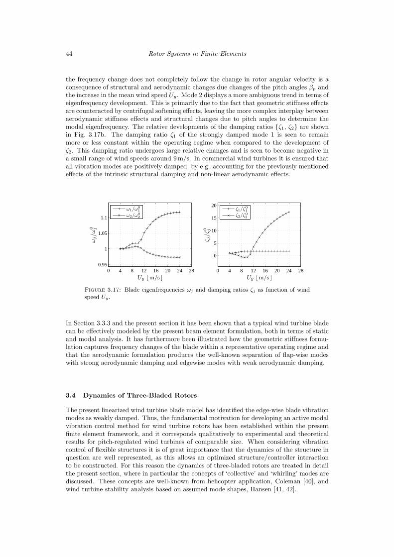
44 Rotor Systems in Finite Elements
the frequency change does not completely follow the change in rotor angular velocity is aconsequence of structural and aerodynamic changes due changes of the pitch angles βp andthe increase in the mean wind speed Uy. Mode 2 displays a more ambiguous trend in terms ofeigenfrequency development. This is primarily due to the fact that geometric stiffness effectsare counteracted by centrifugal softening effects, leaving the more complex interplay betweenaerodynamic stiffness effects and structural changes due to pitch angles to determine themodal eigenfrequency. The relative developments of the damping ratios {ζ1, ζ2} are shownin Fig. 3.17b. The damping ratio ζ1 of the strongly damped mode 1 is seen to remainmore or less constant within the operating regime when compared to the development ofζ2. This damping ratio undergoes large relative changes and is seen to become negative ina small range of wind speeds around 9m/s. In commercial wind turbines it is ensured thatall vibration modes are positively damped, by e.g. accounting for the previously mentionedeffects of the intrinsic structural damping and non-linear aerodynamic effects.
0 4 8 12 16 20 24 280.95
1
1.05
1.1
ω1/ω0
1
ω2/ω0
2
0 4 8 12 16 20 24 28
0
5
10
15
20
ζ1/ζ0
1
ζ2/ζ0
2
Uy [m/s ]Uy [m/s ]
ωj/ω
0 j
ζ j/ζ0 j
Figure 3.17: Blade eigenfrequencies ωj and damping ratios ζj as function of windspeed Uy.
In Section 3.3.3 and the present section it has been shown that a typical wind turbine bladecan be effectively modeled by the present beam element formulation, both in terms of staticand modal analysis. It has furthermore been illustrated how the geometric stiffness formu-lation captures frequency changes of the blade within a representative operating regime andthat the aerodynamic formulation produces the well-known separation of flap-wise modeswith strong aerodynamic damping and edgewise modes with weak aerodynamic damping.
3.4 Dynamics of Three-Bladed Rotors
The present linearized wind turbine blade model has identified the edge-wise blade vibrationmodes as weakly damped. Thus, the fundamental motivation for developing an active modalvibration control method for wind turbine rotors has been established within the presentfinite element framework, and it corresponds qualitatively to experimental and theoreticalresults for pitch-regulated wind turbines of comparable size. When considering vibrationcontrol of flexible structures it is of great importance that the dynamics of the structure inquestion are well represented, as this allows an optimized structure/controller interactionto be constructed. For this reason the dynamics of three-bladed rotors are treated in detailthe present section, where in particular the concepts of ‘collective’ and ‘whirling’ modes arediscussed. These concepts are well-known from helicopter application, Coleman [40], andwind turbine stability analysis based on assumed mode shapes, Hansen [41, 42].
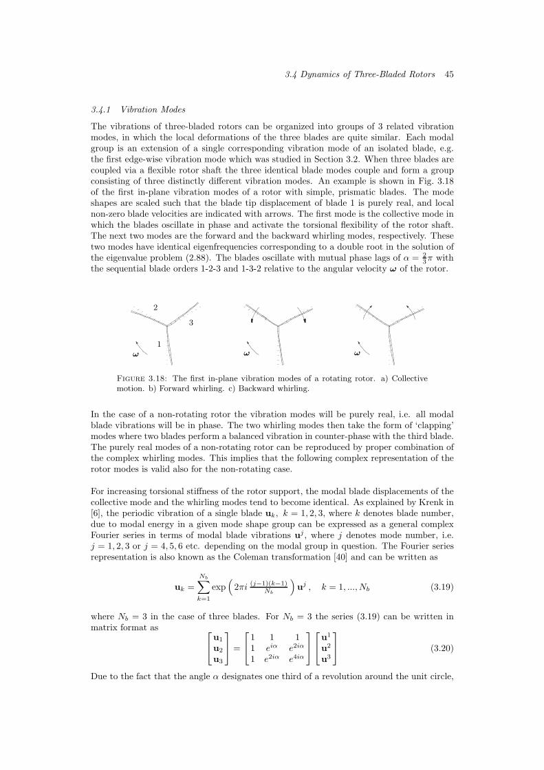
3.4 Dynamics of Three-Bladed Rotors 45
3.4.1 Vibration Modes
The vibrations of three-bladed rotors can be organized into groups of 3 related vibrationmodes, in which the local deformations of the three blades are quite similar. Each modalgroup is an extension of a single corresponding vibration mode of an isolated blade, e.g.the first edge-wise vibration mode which was studied in Section 3.2. When three blades arecoupled via a flexible rotor shaft the three identical blade modes couple and form a groupconsisting of three distinctly different vibration modes. An example is shown in Fig. 3.18of the first in-plane vibration modes of a rotor with simple, prismatic blades. The modeshapes are scaled such that the blade tip displacement of blade 1 is purely real, and localnon-zero blade velocities are indicated with arrows. The first mode is the collective mode inwhich the blades oscillate in phase and activate the torsional flexibility of the rotor shaft.The next two modes are the forward and the backward whirling modes, respectively. Thesetwo modes have identical eigenfrequencies corresponding to a double root in the solution ofthe eigenvalue problem (2.88). The blades oscillate with mutual phase lags of α = 2
3π withthe sequential blade orders 1-2-3 and 1-3-2 relative to the angular velocity ω of the rotor.
1
2
3
ωωω
Figure 3.18: The first in-plane vibration modes of a rotating rotor. a) Collectivemotion. b) Forward whirling. c) Backward whirling.
In the case of a non-rotating rotor the vibration modes will be purely real, i.e. all modalblade vibrations will be in phase. The two whirling modes then take the form of ‘clapping’modes where two blades perform a balanced vibration in counter-phase with the third blade.The purely real modes of a non-rotating rotor can be reproduced by proper combination ofthe complex whirling modes. This implies that the following complex representation of therotor modes is valid also for the non-rotating case.
For increasing torsional stiffness of the rotor support, the modal blade displacements of thecollective mode and the whirling modes tend to become identical. As explained by Krenk in[6], the periodic vibration of a single blade uk, k = 1, 2, 3, where k denotes blade number,due to modal energy in a given mode shape group can be expressed as a general complexFourier series in terms of modal blade vibrations uj , where j denotes mode number, i.e.j = 1, 2, 3 or j = 4, 5, 6 etc. depending on the modal group in question. The Fourier seriesrepresentation is also known as the Coleman transformation [40] and can be written as
uk =
Nb∑
k=1
exp(
2πi (j−1)(k−1)Nb
)
uj , k = 1, ..., Nb (3.19)
where Nb = 3 in the case of three blades. For Nb = 3 the series (3.19) can be written inmatrix format as
u1
u2
u3
=
1 1 11 eiα e2iα
1 e2iα e4iα
u1
u2
u3
(3.20)
Due to the fact that the angle α designates one third of a revolution around the unit circle,

46 Rotor Systems in Finite Elements
the Fourier representation (3.20) can be written in the slightly different form
u1
u2
u3
=
1 1 11 eiα e−iα
1 e−iα eiα
u1
u2
u3
(3.21)
From this format it can be directly established that the resulting motion of the three bladesis the sum of a collective blade motion and two whirling motions. This is seen by writing(3.21) as the sum
u1
u2
u3
=
111
u1 +
1eiα
e−iα
u2 +
1e−iα
eiα
u3 (3.22)
The first term represents the collective blade motion and the last two terms represent thebackward and forward whirling modes, respectively.
In a transient load case of a wind turbine rotor, all terms in (3.22) will be present in the struc-tural response. As shown in Section 3.3 the edge-wise vibration modes are subject to weakaerodynamic damping, and this makes these modes an obvious target for resonant vibrationcontrol. Due to the inherent difference in natural frequency between the collective and thewhirling modes, two separate resonant controllers with different frequency calibrations arerequired in order to perform a full and optimal control of the first edge-wise vibration modegroup. It is therefore necessary to be able to filter out the collective blade motion and thewhirling blade motion, respectively, from any measured broad-band rotor response. For thispurpose the collective blade motion u1 is conveniently seen to correspond exactly to themean value of the three physical blade responses uj ,
u1 = 13
(
u1 + u2 + u3
)
(3.23)
which follows directly from summation over uj in (3.21). Thus, the collective mode can beobserved directly as the mean value of the three blade responses. The signal associated witha pair of whirling modes is identified by subtracting the mean blade response from the fullblade response,
u′
1
u′
2
u′
3
=
u1
u2
u3
−
111
u1 =1
3
2u1 − u2 − u3
−u1 + 2u2 − u3
−u1 − u2 + 2u3
(3.24)
which produces the ‘deviatoric’ blade deformations u′
k. As noted by Krenk [43] the conceptof a deviatoric part of a response is similar to the concept of deviatoric stresses in con-tinuum mechanics, see e.g. Timoshenko & Goodier [44]. The identification of the signalsrepresenting the collective mode (3.23) and the whirling modes (3.24) is applied directly inthe controller formulation in Chapter 4.
In the next section the dynamics of whirling in three-bladed rotors are discussed. Theanalysis is based on the first in-plane forward whirling mode of a rotor with simple, prismaticblades of homogenous material and no coning. However, the principles apply generally, notleast to the first edge-wise whirling modes of a wind turbine rotor as will be demonstratedin Section 3.5.
3.4.2 Dynamics of Whirling
Whirling is a gyroscopic phenomenon occurring in rotating structures, e.g. transmissionshafts or bladed rotors. As seen above, whirling modes come in pairs of forward and back-ward whirling and the difference between the two lies in the sign of the phase lag betweengyroscopic and inertial forces. The interplay between the gyroscopic and inertial forces is

3.4 Dynamics of Three-Bladed Rotors 47
conveniently analyzed by a full complex representation of the blade displacement compo-nents. In Fig. 3.19 the local in-plane blade tip displacements {q1z , q2z , q3z} and their velocityand acceleration counterparts are plotted in the complex plane for the forward whirlingmode. The mode is scaled in terms of phase and amplitude such that the tip displacementof blade 1 is purely imaginary with negative unit amplitude. For progressing time the pointsare rotated counter-clockwise as indicated in the figure, and this corresponds to the bladespassing through identical states in the sequential order 1-2-3 with a phase difference of 2
3π.The chosen scale of the mode implies that the velocity of blade 1 is purely real and positive.
Re[ qjz ]
Im[ qjz ]
iωntiωntiωntq1z
q2z q3z
Re[ ˙qjz ]
Im[ ˙qjz ]
˙q1z
˙q3z
˙q2z
Re[ ¨qjz ]
Im[ ¨qjz ]
¨q1z
¨q3z
¨q2z
Figure 3.19: Local forward whirling blade tip displacements, velocities and acceler-ations.
In Fig. 3.20 the real parts of the structural displacements are plotted. Blade 1 is seento be undeformed while blades 2 and 3 have negative and positive local displacements,respectively. The direction of the angular velocity of the rotor ωy is shown in the figure, andthe aforementioned sequential order 1-2-3 of identical blade states propagates in the samecircular direction. This explains the term ‘forward whirling’ whereas ‘backward whirling’corresponds to the sequential order 1-3-2 for the present case.
˙q1z
˙q3z
˙q2z
f1
G
f2
G f3
M
f3
Gf2
M
ωy
¨q3z
¨q2z
Figure 3.20: Forward whirling with local blade velocities and accelerations andresulting hub forces.
The real parts of blade tip velocities { ˙q1z , ˙q2z , ˙q3z} and accelerations { ¨q1z , ¨q2z , ¨q3z} are depictedin Fig. 3.20 by vector representations indicating directions and amplitudes. Also, the gyro-scopic blade root forces {f1
G, f2G, f
3G} as well as the acceleration-proportional inertial forces
{f2M , f3
M} are plotted. The gyroscopic forces are parallel with the local blade axes and dueto the symmetry of the system these have a common resultant purely in the opposite direc-tion of the reference axis of blade 1. The flexible support of the rotor is deformed under this

48 Rotor Systems in Finite Elements
loading, by which the gyroscopic coupling of the blades is established. The acceleration-proportional blade root forces are symmetric about the axis of blade 1 and perpendicularto their local blade axes. In the case of forward whirling these contribute positively to thegyroscopic resultant whereas the contribution is negative for backward whirling. Thus, for-ward whirling will be the mode which produces the dominating in-plane loads of the mainrotor shaft.
A simple example is given in the following to demonstrate the effects described above. Arotor is modeled using three rectangular, prismatic 8m blades of homogeneous material. Theblade have the cross-section width wb = 0.035m and the cross-section heights hb = 0.200m,material density = 2700kg/m2, elastic modulus E = 72GPa and a Poisson ratio ofν = 0.35. The blades are oriented such that in-plane displacements correspond to bendingpurely about the strong blade axes, and the local blade reference axis coincides with thelongitudinal axis of symmetry. No aerodynamics are included. The eigenvalue problem(2.88) is solved for stationary rotation at the angular velocity ωy = 5 rad/s and modes 5and 6 are the forward and backward whirling modes respectively, with the eigenfrequencies{ω5, ω6} = {16.5105 rad/s, 16.5110 rad/s}. The fourth decimal reveals that the numericalsolution of the eigenvalue problem does not produce eigenfrequencies which are exactlyequal. Mode 4 is the first ‘collective’ in-plane vibration mode, in which all blades oscillate inphase, and it has the eigenfrequency ω4 = 16.0163 rad/s. Modes 1-3 are the first out-of-planecollective and whirling modes.
0 2 4 6 8
−1
−0.5
0
Re(uj)Im(uj)u5
u6
0 2 4 6 8
−15
−10
−5
0
x 10−5
0 2 4 6 8−1
−0.5
0
0.5
1
0 2 4 6 8−1
0
1
x 10−4
x [ m ]x [ m ]
x [ m ]x [ m ]
q1 z q1 x
q2 z q2 x
(a) (b)
(c) (d)
Figure 3.21: Local in-plane (qjz) and axial (qjx) displacements for forward and back-ward whirling.
The mode shapes u5 and u6 are plotted together in Fig. 3.21 in terms of local deformationsof blade 1 and the modes are scaled as in Fig. 3.19. The real parts are plotted in black andthe imaginary parts are plotted in blue. Nodal values of u5 are indicated with × while nodalvalues of u6 are indicated with +. The in-plane displacements q1z are seen in Fig. 3.21a tobe identical for the two modes. In Fig. 3.21b the axial deformations q1x of the two modes areseen to develop identically, but a constant offset is seen between them. This offset is due tothe displacement of the rotor, which identifies the difference between forward and backwardwhirling. For completeness, the local displacements of q2z and q2x of blade 2 are shown inFig. 3.21c and d. In both cases the displacements are seen to have the same phases and
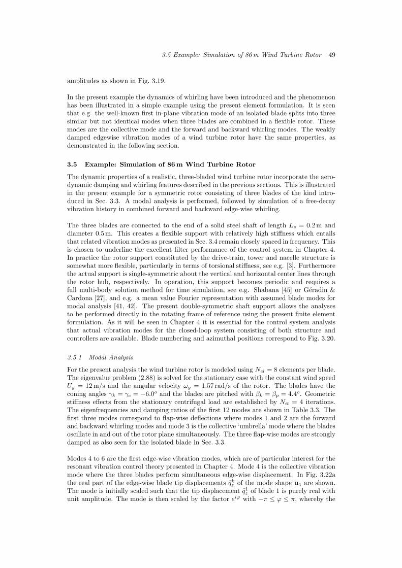
3.5 Example: Simulation of 86m Wind Turbine Rotor 49
amplitudes as shown in Fig. 3.19.
In the present example the dynamics of whirling have been introduced and the phenomenonhas been illustrated in a simple example using the present element formulation. It is seenthat e.g. the well-known first in-plane vibration mode of an isolated blade splits into threesimilar but not identical modes when three blades are combined in a flexible rotor. Thesemodes are the collective mode and the forward and backward whirling modes. The weaklydamped edgewise vibration modes of a wind turbine rotor have the same properties, asdemonstrated in the following section.
3.5 Example: Simulation of 86m Wind Turbine Rotor
The dynamic properties of a realistic, three-bladed wind turbine rotor incorporate the aero-dynamic damping and whirling features described in the previous sections. This is illustratedin the present example for a symmetric rotor consisting of three blades of the kind intro-duced in Sec. 3.3. A modal analysis is performed, followed by simulation of a free-decayvibration history in combined forward and backward edge-wise whirling.
The three blades are connected to the end of a solid steel shaft of length Ls = 0.2m anddiameter 0.5m. This creates a flexible support with relatively high stiffness which entailsthat related vibration modes as presented in Sec. 3.4 remain closely spaced in frequency. Thisis chosen to underline the excellent filter performance of the control system in Chapter 4.In practice the rotor support constituted by the drive-train, tower and nacelle structure issomewhat more flexible, particularly in terms of torsional stiffness, see e.g. [3]. Furthermorethe actual support is single-symmetric about the vertical and horizontal center lines throughthe rotor hub, respectively. In operation, this support becomes periodic and requires afull multi-body solution method for time simulation, see e.g. Shabana [45] or Geradin &Cardona [27], and e.g. a mean value Fourier representation with assumed blade modes formodal analysis [41, 42]. The present double-symmetric shaft support allows the analysesto be performed directly in the rotating frame of reference using the present finite elementformulation. As it will be seen in Chapter 4 it is essential for the control system analysisthat actual vibration modes for the closed-loop system consisting of both structure andcontrollers are available. Blade numbering and azimuthal positions correspond to Fig. 3.20.
3.5.1 Modal Analysis
For the present analysis the wind turbine rotor is modeled using Nel = 8 elements per blade.The eigenvalue problem (2.88) is solved for the stationary case with the constant wind speedUy = 12m/s and the angular velocity ωy = 1.57 rad/s of the rotor. The blades have theconing angles γk = γc = −6.0o and the blades are pitched with βk = βp = 4.4o. Geometricstiffness effects from the stationary centrifugal load are established by Nit = 4 iterations.The eigenfrequencies and damping ratios of the first 12 modes are shown in Table 3.3. Thefirst three modes correspond to flap-wise deflections where modes 1 and 2 are the forwardand backward whirling modes and mode 3 is the collective ‘umbrella’ mode where the bladesoscillate in and out of the rotor plane simultaneously. The three flap-wise modes are stronglydamped as also seen for the isolated blade in Sec. 3.3.
Modes 4 to 6 are the first edge-wise vibration modes, which are of particular interest for theresonant vibration control theory presented in Chapter 4. Mode 4 is the collective vibrationmode where the three blades perform simultaneous edge-wise displacement. In Fig. 3.22athe real part of the edge-wise blade tip displacements qkz of the mode shape u4 are shown.The mode is initially scaled such that the tip displacement q1z of blade 1 is purely real withunit amplitude. The mode is then scaled by the factor eiϕ with −π ≤ ϕ ≤ π, whereby the
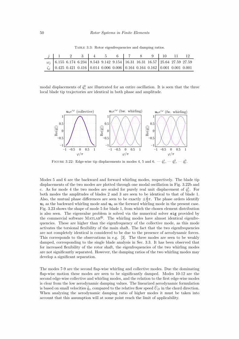
50 Rotor Systems in Finite Elements
Table 3.3: Rotor eigenfrequencies and damping ratios.
j 1 2 3 4 5 6 7 8 9 10 11 12
ωj 6.155 6.174 6.234 8.543 9.142 9.154 16.31 16.31 16.57 25.64 27.59 27.59
ζj 0.425 0.421 0.416 0.014 0.006 0.006 0.164 0.164 0.162 0.001 0.001 0.001
modal displacements of qkz are illustrated for an entire oscillation. It is seen that the threelocal blade tip trajectories are identical in both phase and amplitude.
−1 −0.5 0 0.5 1−1
−0.5
0
0.5
1
−1 −0.5 0 0.5 1−1
−0.5
0
0.5
1
−1 −0.5 0 0.5 1−1
−0.5
0
0.5
1
ϕ/πϕ/πϕ/π
Re(qj z)
Re(qj z)
Re(qj z)
u4eiϕ (collective) u5e
iϕ (bw. whirling) u6eiϕ (fw. whirling)
Figure 3.22: Edge-wise tip displacements in modes 4, 5 and 6. — q1z , — q2z , — q3z .
Modes 5 and 6 are the backward and forward whirling modes, respectively. The blade tipdisplacements of the two modes are plotted through one modal oscillation in Fig. 3.22b andc. As for mode 4 the two modes are scaled for purely real unit displacement of q1z . Forboth modes the amplitudes of blades 2 and 3 are seen to be identical to that of blade 1.Also, the mutual phase differences are seen to be exactly ± 2
3π. The phase orders identifyu5 as the backward whirling mode and u6 as the forward whirling mode in the present case.Fig. 3.23 shows the shape of mode 5 for blade 1, from which the chosen element distributionis also seen. The eigenvalue problem is solved via the numerical solver eig provided bythe commercial software Matlabr. The whirling modes have almost identical eigenfre-quencies. These are higher than the eigenfrequency of the collective mode, as this modeactivates the torsional flexibility of the main shaft. The fact that the two eigenfrequenciesare not completely identical is considered to be due to the presence of aerodynamic forces.This corresponds to the observations in e.g. [3]. The three modes are seen to be weaklydamped, corresponding to the single blade analysis in Sec. 3.3. It has been observed thatfor increased flexibility of the rotor shaft, the eigenfrequencies of the two whirling modesare not significantly separated. However, the damping ratios of the two whirling modes maydevelop a significant separation.
The modes 7-9 are the second flap-wise whirling and collective modes. Due the dominatingflap-wise motion these modes are seen to be significantly damped. Modes 10-12 are thesecond edge-wise collective and whirling modes, and the relation to the first edge-wise modesis clear from the low aerodynamic damping values. The linearized aerodynamic formulationis based on small velocities ˙qD compared to the relative flow speed UD in the chord direction.When analyzing the aerodynamic damping ratio of higher modes it must be taken intoaccount that this assumption will at some point reach the limit of applicability.

3.5 Example: Simulation of 86m Wind Turbine Rotor 51
0 5 10 15 20 25 30 35 40 45
00.20.40.60.8
1
Re(u1
5)
Im(u1
5)
0 5 10 15 20 25 30 35 40 45
0
0.1
0.2
0.3
0.4
x [m ]x [m ]
q1 z q1 y
Figure 3.23: The edge-wise backward whirling mode u1
5 for blade 1 with respect tothe local blade coordinate system.
3.5.2 Free Vibration
In this section a simple example of simulated transient rotor behavior is given. The purposeis to extend the introduction to the edge-wise whirling modes and to show that these arecorrectly reproduced by the time integration algorithm given in Table 3.2. The time step his selected such that mode 16 of the coupled structure is resolved with 10 points per period,corresponding to h = 0.023 s. In each time instant the geometric stiffness matrix Kg isestablished using four iterations of internal stresses in the dynamic equilibrium of (2.76).The rotor angular velocity is held constant at ωy = 1.57 rad/s and the blade pitch anglesare held constant at βp = 4.4o.
The initial conditions of the free vibration history are chosen such that the edge-wise forwardand backward whirling modes are initiated with relatively high energy levels. Blade num-bering and azimuthal angles in the rotor coordinate system is identical to the rotor shownin Fig. 3.20. The initial conditions of the rotor correspond to the stationary centrifugal andaerodynamic load case which is used as basis for the modal analysis above, supplementedby a constant external load. The external load corresponds to a somewhat realistic situa-tion where blade 2 and blade 3 are connected by a taut string attached in the local bladeradii x/L = 0.87. The load vector is defined by specifying the loads Q 2,3
z = ±104 kNm inthe corresponding nodes. The transient response is initiated by ‘cutting the string’, mod-eled by setting the two nodal forces to zero, Q 2,3
z = 0, during the course of a single time step.
The structural response is shown in Fig. 3.24a in terms of the three in-plane blade tipresponses in the rotor system qkz . At t = 0.2 s the string is cut and blades 2 and 3 areseen to start oscillating about a new equilibrium, corresponding to the remaining stationarycentrifugal and aerodynamic load. Blade 1 is seen to be almost unaffected by the abruptload change.
In Fig. 3.24b the local edge-wise tip responses qkz are shown. These are evaluated by pre-multiplication of the blade state vectors uk by RT
k defined in (3.7). The rotor symmetry isevident when observing the local blade states, as these have identical stationary equilibriaunder pure centrifugal and aerodynamic load. Thus, the behavior of the blades is directlycomparable when observed in the local blade coordinate systems. Blades 2 and 3 are seento perform a ‘clapping’ motion which can be shown to correspond to a symmetric energydistribution between the forward and backward whirling modes. In the present case theinitial ‘string’ load does not purely excite the first edge-wise vibration modes, by which theobserved clapping motion is not perfectly symmetric.
The energy density spectrum S2q (ω) of the local edge-wise displacements q2z of blade 2 is
shown in Fig. 3.25. The spectrum is normalized with its maximum value S0q corresponding
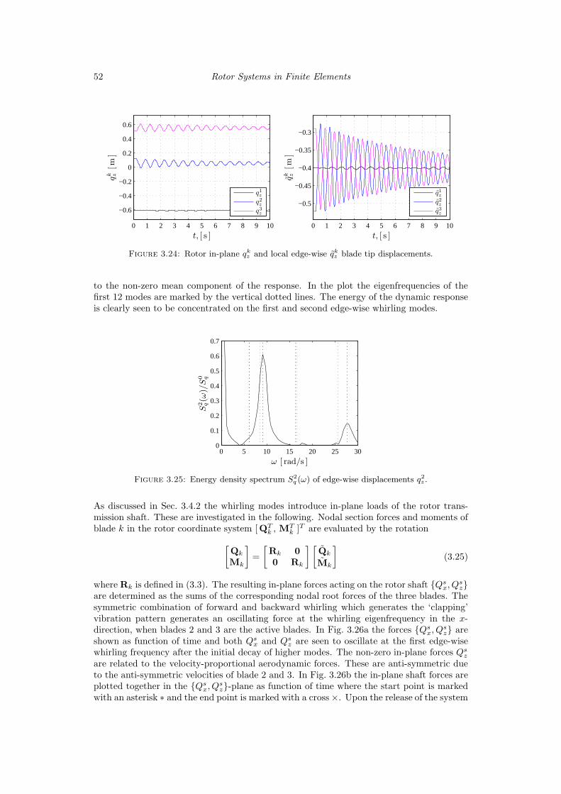
52 Rotor Systems in Finite Elements
0 1 2 3 4 5 6 7 8 9 10
−0.6
−0.4
−0.2
0
0.2
0.4
0.6
q1
z
q2
z
q3
z
0 1 2 3 4 5 6 7 8 9 10
−0.5
−0.45
−0.4
−0.35
−0.3
q1
z
q2
z
q3
z
t, [ s ]t, [ s ]
qk z[m
]
qk z[m
]
Figure 3.24: Rotor in-plane qkz and local edge-wise qkz blade tip displacements.
to the non-zero mean component of the response. In the plot the eigenfrequencies of thefirst 12 modes are marked by the vertical dotted lines. The energy of the dynamic responseis clearly seen to be concentrated on the first and second edge-wise whirling modes.
0 5 10 15 20 25 300
0.1
0.2
0.3
0.4
0.5
0.6
0.7
ω [ rad/s ]
S2 q(ω
)/S
0 q
Figure 3.25: Energy density spectrum S2
q (ω) of edge-wise displacements q2z .
As discussed in Sec. 3.4.2 the whirling modes introduce in-plane loads of the rotor trans-mission shaft. These are investigated in the following. Nodal section forces and moments ofblade k in the rotor coordinate system [QT
k , MTk ]T are evaluated by the rotation
[
Qk
Mk
]
=
[
Rk 00 Rk
] [
Qk
Mk
]
(3.25)
where Rk is defined in (3.3). The resulting in-plane forces acting on the rotor shaft {Qsx, Q
sz}
are determined as the sums of the corresponding nodal root forces of the three blades. Thesymmetric combination of forward and backward whirling which generates the ‘clapping’vibration pattern generates an oscillating force at the whirling eigenfrequency in the x-direction, when blades 2 and 3 are the active blades. In Fig. 3.26a the forces {Qs
x, Qsz} are
shown as function of time and both Qsx and Qs
z are seen to oscillate at the first edge-wisewhirling frequency after the initial decay of higher modes. The non-zero in-plane forces Qs
z
are related to the velocity-proportional aerodynamic forces. These are anti-symmetric dueto the anti-symmetric velocities of blade 2 and 3. In Fig. 3.26b the in-plane shaft forces areplotted together in the {Qs
x, Qsz}-plane as function of time where the start point is marked
with an asterisk ∗ and the end point is marked with a cross×. Upon the release of the system

3.5 Example: Simulation of 86m Wind Turbine Rotor 53
the resulting in-plane force is seen to quickly engage in an elliptical clock-wise motion. TheQs
x-components are due to the gyroscopic forces and acceleration-proportional inertial forcesof the whirling modes and the Qs
z components arise from the aerodynamic damping term.The simulation end point × is taken when the displacements of blade 2 and 3 are closeto zero, corresponding the blades moving at the maximal local velocities. This is seen inFig. 3.26a and to correspond to a maximum of Qs
z.
0 1 2 3 4 5 6 7 8 9 10−2
−1
0
1
2x 10
4
Qs
x
Qsz
−2 −1 0 1 2
x 104
−2
−1
0
1
2x 10
4
t, [ s ]
Qs x,Q
s z[N
]
Qsx [ N ]
Qs z[N
]
Figure 3.26: Global blade root section forces Qsx and Qs
z.
The present section concludes the fundamental structural and aerodynamic analysis of thethree-bladed wind turbine rotor. By a simple example it has been illustrated that thethree-bladed wind turbine rotor model with symmetric pitch and coning angles and thenon-symmetric aerodynamic formulation reproduces the weakly damped edge-wise vibrationmodes in a time integration of the equations of motion. Due to the presence of gyroscopicforces these modes are divided into a collective mode in which the blades oscillate in phase,and into the forward and backward whirling modes.

Chapter 4
Resonant Vibration Control of Beams and Rotors
In this chapter the basic idea of the resonant controller and its expansion to flexible multi-degree-of-freedom systems is given. Subsequently the formats for application to stationarysystems and gyroscopics systems are given, accompanied by application to an isolated 42mblade and an 86m wind turbine rotor.
4.1 Basic Idea of the Resonant Controller
In this section the basic format of a resonant vibration controller for an undamped single-degree-of-freedom system is introduced. Also, the expansion to multi-degree-of-freedomsystems is briefly discussed. The format is adopted from Krenk & Høgsberg [15, 16] wherealso the calibration scheme for the controller parameters is developed. The basic single-degree-of-freedom system is shown in Fig. 4.1a, with mass m, stiffness k and displacementx.
fe
fη
x
mk
0.7 0.8 0.9 1 1.1 1.2 1.30
2
4
6
8
10
12FreeCtr.
ω/ω0
x/xst
Figure 4.1: Basic, active resonant vibration control. a) Single-degree-of-freedomsystem. b) Frequency response.
If the free structural system is subjected to a broad band external force fe, resonant ampli-fication of the response occurs near the structural eigenfrequency ω0 = k/m. This amplifi-cation is shown with a dashed line in Fig. 4.1b where the stationary response amplitude xcorresponding to a harmonic load of the form fe(t) = fee
iωt is shown, normalized with thestatic response xst.
The fundamental objective of the resonant controller is to reduce the dynamic amplificationof the structural response near ω0 by actively applying a load fη to the structure. For thispurpose the controller is defined as a second order filter with a natural frequency ωs close tothe structural eigenfrequency ω0. The independent controller state variable is excited by asensor filter, transferring structural feedback in terms of e.g. displacement x or accelerationx, and the controller affects the structure via an actuator filter transferring the physicalload. This creates a closed-loop system where resonant structural activity invokes resonantcontroller activity. By including a damping term in the controller transfer function, themechanical energy of the coupled system can be effectively dissipated and structural dis-placements significantly reduced. For optimal calibration of the controller properties, the
54

4.1 Basic Idea of the Resonant Controller 55
targeted structural mode splits into two equally damped modes, closely spaced around theoriginal structural frequency ω0. The frequency response of a coupled system with an op-timally calibrated controller is shown in Fig. 4.1b in terms of the fully drawn curve. Theequal damping of the two emanating modes is seen to produce two identical resonant peakswith low amplification.
The coupled equations of motion for the single-degree-of-freedom system and the resonantcontroller are shown in (4.1) and (4.2). The equations are shown in the frequency domain,corresponding to a harmonic load fe(t) = fee
iωt with associated stationary response x(t) =xeiωt. The structural equation of motion is
G sxx(ω)x+G s
xη(ω)η = fe/m (4.1)
where Gxx(ω) = ω20 − ω2 is the transfer function of the free, undamped structure and
G sxη(ω) is the actuator feedback transfer function. Thus, the controller feedback is given
as fη = G sxη(ω)η where η is the controller state variable. This variable is governed by the
equationG s
ηx(ω)x+G sηη(ω)η = 0 (4.2)
where G sηx(ω) is the sensor transfer function and G s
ηη(ω) is the second order controllertransfer function, defined as
G sηη(ω) = ω2
s − ω2 + 2iζsωsω (4.3)
where ωs is the controller eigenfrequency and ζs is the controller damping ratio. Krenk &Høgsberg [15, 16] define the following sensor and actuator transfer functions for a controllerwith acceleration feedback,
G sηx(ω) = ω2, G s
xη(ω) = αsω2s + βs2iζsωsω (4.4)
The sensor feedback transfer function G sηx(ω) is seen to be a differential operator and the
actuator transfer function G sxη(ω) is a linear filter with the two gain parameters αs and βs.
In [15, 16] a displacement-based feedback system is also defined, which is not included here.For both acceleration and displacement feedback an optimal and explicit calibration schemeis developed in [15, 16]. The derivation is performed in two steps. The optimal controllerfrequency ωs is initially identified by requiring equal damping of the two emanating modes.The remaining parameters are then determined by invoking a characteristic restriction onthe dip in dynamic amplification close to ω0, which has the effect of flattening and therebylowering the entire resonant plateau of the coupled system. The optimal parameters areexplicitly given as
αs =2ζ2s
1− 2ζ2s, βs = αs, ωs =
ω0
1 + αs(4.5)
The acceleration feedback filters (4.3) and (4.4) are equivalent to those of the passive, me-chanical tuned mass damper [8, 46] when the gain parameters αs, βs are equal to the massratio between structure and damper. As shown in [46] the resulting damping ratios ∆ζbecome close to half the damping ratio of the damper, i.e. for a desired additional dampingratio ∆ζ the basic controller damping ratio is chosen as ζs = 2∆ζ.
The resonant controller format can be applied to multi-degree-of-freedom systems. Theformat used in the present case is given in the frequency domain as
(
K+ iω2G− ω2M)
u+ fη = fe (4.6)
where fη represents the imposed load from the actuator system. When the resonant controlformat is applied to a multi-degree-of-freedom system for vibration suppression of selected

56 Resonant Vibration Control of Beams and Rotors
modes, a number of physical considerations concerning the interplay between the controlsystem and the modal dynamics of the flexible structure comes into play. One is that thesensor/acutator system must be positioned such that good controllability and observabilityis obtained for the targeted mode. For the present collocated format these two concepts arerepresented in the term modal connectivity. Also, it is necessary to minimize the controllerconnectivity to other modes, as these will otherwise disturb the calibration and operationof the controller. The resonant characteristic of the resonant controller provides and ef-fective decoupling from other modes when these are well separated in frequency from thetargeted mode. In this case the response of higher modes will be limited in the resonantregion of the targeted mode, and their contribution can be approximated and included bya quasi-static approximation, see Preumont [35] and Krenk & Høgsberg [15, 16]. Also, ageometric decoupling from other modes can be obtained in systems where mode shapes aregeometrically orthogonal, e.g. for beam bending modes about the strong and weak axis,respectively. In the case of gyroscopic systems, and in particular three-bladed rotors, modesarise which are closely spaced both frequency-wise and geometrically. These are discussed inChapter 3 as the groups consisting of one collective vibration mode and the backward andforward whirling modes. In addition to the considered modal decoupling methods for rotat-ing beams, optimal resonant control of the three-bladed rotor modes requires an additionaldecoupling scheme based on the mean and deviatoric blade deformation patterns describedin Chapter 3. In Sec. 4.2 resonant vibration control of rotating beams is discussed and inSec. 4.3 resonant vibration control of three-bladed rotors is discussed.
4.2 Control of Rotating Beams
In this section an overview of the controller format for control of non-rotating multi-degree-of-freedom structures is given, followed by an example where the method is applied to anisolated wind turbine blade. The blade is rotating, which gives rise to an eigenfrequencychange compared to the stand-still situation, necessary for the controller tuning. As theblade is isolated the gyroscopic effects play a minor role, and the calibration according tothe method for non-rotating structures proves effective. To illustrate that two modes can beaddressed simultaneously with two different controller systems with associated sensor/actu-ator pairs, both the first flap-wise and the first edge-wise mode is controlled.
4.2.1 Controller Format
For a system with multiple controllers with associated sensor/actuator pairs, the combinedactuator force fη takes the form
fη = w1η1G1xη(ω) +w2η2G
2xη(ω) + ... (4.7)
where the first term is the actuator feedback from controller 1, the second term is that fromcontroller 2 etc. The vectors wk are the physical connectivity vectors of the collocated sen-sor/actuator pairs. A method for establishing the connectivity vector for a three-dimensionalbeam is given in Appedix C. The components ηk are the controller states and G k
xη(ω) arethe actuator feedback transfer function, corresponding to G s
xη(ω) for the basic case. Eachcontroller state is governed by the equation
G kηη(ω)ηk +G k
ηx(ω)wTk u (4.8)
where wTk u provides a scalar feedback from the structural deformation state. For an active
strut positioned as in Fig. 1.2, i.e. in the axial direction with a finite distance to the elasticcenter, this feedback represents a combined state of axial blade deformation and bending.The controller filter is defined as the second order filter
G kηη(ω) = ω2
k − ω2 + 2iζkωkω (4.9)
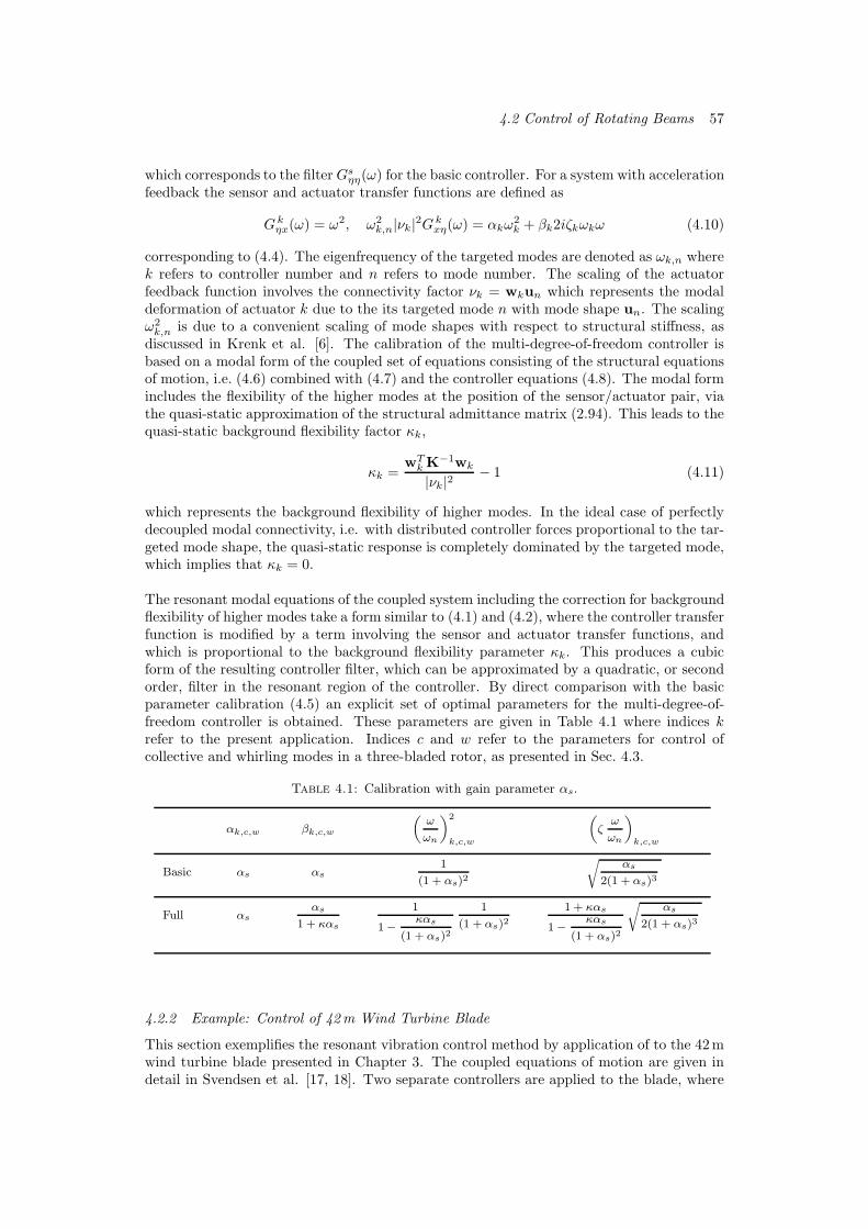
4.2 Control of Rotating Beams 57
which corresponds to the filterGsηη(ω) for the basic controller. For a system with acceleration
feedback the sensor and actuator transfer functions are defined as
G kηx(ω) = ω2, ω2
k,n|νk|2G kxη(ω) = αkω
2k + βk2iζkωkω (4.10)
corresponding to (4.4). The eigenfrequency of the targeted modes are denoted as ωk,n wherek refers to controller number and n refers to mode number. The scaling of the actuatorfeedback function involves the connectivity factor νk = wkun which represents the modaldeformation of actuator k due to the its targeted mode n with mode shape un. The scalingω2k,n is due to a convenient scaling of mode shapes with respect to structural stiffness, as
discussed in Krenk et al. [6]. The calibration of the multi-degree-of-freedom controller isbased on a modal form of the coupled set of equations consisting of the structural equationsof motion, i.e. (4.6) combined with (4.7) and the controller equations (4.8). The modal formincludes the flexibility of the higher modes at the position of the sensor/actuator pair, viathe quasi-static approximation of the structural admittance matrix (2.94). This leads to thequasi-static background flexibility factor κk,
κk =wT
k K−1wk
|νk|2− 1 (4.11)
which represents the background flexibility of higher modes. In the ideal case of perfectlydecoupled modal connectivity, i.e. with distributed controller forces proportional to the tar-geted mode shape, the quasi-static response is completely dominated by the targeted mode,which implies that κk = 0.
The resonant modal equations of the coupled system including the correction for backgroundflexibility of higher modes take a form similar to (4.1) and (4.2), where the controller transferfunction is modified by a term involving the sensor and actuator transfer functions, andwhich is proportional to the background flexibility parameter κk. This produces a cubicform of the resulting controller filter, which can be approximated by a quadratic, or secondorder, filter in the resonant region of the controller. By direct comparison with the basicparameter calibration (4.5) an explicit set of optimal parameters for the multi-degree-of-freedom controller is obtained. These parameters are given in Table 4.1 where indices krefer to the present application. Indices c and w refer to the parameters for control ofcollective and whirling modes in a three-bladed rotor, as presented in Sec. 4.3.
Table 4.1: Calibration with gain parameter αs.
αk,c,w βk,c,w
(
ω
ωn
)
2
k,c,w
(
ζω
ωn
)
k,c,w
Basic αs αs1
(1 + αs)2
√
αs
2(1 + αs)3
Full αsαs
1 + καs
1
1−
καs
(1 + αs)2
1
(1 + αs)21 + καs
1−
καs
(1 + αs)2
√
αs
2(1 + αs)3
4.2.2 Example: Control of 42m Wind Turbine Blade
This section exemplifies the resonant vibration control method by application of to the 42mwind turbine blade presented in Chapter 3. The coupled equations of motion are given indetail in Svendsen et al. [17, 18]. Two separate controllers are applied to the blade, where

58 Resonant Vibration Control of Beams and Rotors
one targets the first flap-wise mode and the other targets the first edge-wise mode. Thefirst flap-wise mode has significant aerodynamic damping, and in practical wind turbineapplication it would therefore be more relevant to target only edge-wise modes. However,the present example illustrates that it is possible to target several modes with individualcontrol systems and obtain close to optimal controller calibration with the present method.
Two active struts are applied to the wind turbine blades as shown in Fig. 4.2. The strutsare positioned close to the blade root where curvatures due to bending are largest. Thismaximizes the modal connectivities. The positions correspond to strut lengths Lk = 6.0m,in positions between the first two element nodes as shown in [17]. Each strut is positionedsuch that the axis of the strut is parallel with the local blade axis x, in the distance Rk =0.70m from the axis. This defines a circumference of possible strut positions, defined by theangles θk measured from the y-axis.
x
y
z
Qη,1
−Qη,1 Qη,2
−Qη,2
Figure 4.2: The 42m wind turbine blade with two active strut controllers.
In the positioning of the sensor/actutator pairs the objective is generally to obtain a highmodal connectivity while minimizing the background flexibility of higher modes, within theconstraints of practical implementation. When a single controller is applied to a beam thisis a relatively straightforward procedure, as the mode shapes of the free structure providea good approximation of the resulting mode shapes in the controlled structure. This allowsa direct procedure of application based on maximizing ν while minimizing κ. However,when multiple controllers are applied, the interaction between these must be accounted for.The explicit calibration procedure of Table 4.1 directly provides the optimal parametersfor a chosen position of a single controller, and the resulting properties of the full, coupledsystem including all controllers can be directly evaluated by modal analysis. Thus, a simpleparameter study for different combinations of controller positions can be performed and theoptimal combination identified. This is done here with circumferential strut positions θ1and θ2 as variables and the result is seen in Fig. 4.3. The following error measure is used.When the resonant controller is optimally tuned, the targeted mode splits into two newmodes with identical damping ratios ζn,1 and ζn,2. The calibration error ε is defined as therelative deviation of e.g. ζn,1 from the mean value of the two damping ratios. This errormeasure reflects the lack of symmetry in the frequency response curve seen in Fig. 4.1. Itis seen in Fig. 4.3 that the calibration errors εk have a common region in which they areboth minimized, namely for θ1/π ≃ 1.0 and θ2/π ≃ 0.25. These positions are depicted inFig. 4.2 and the result corresponds well to the intuitive notion that controller 1, targetingthe flap-wise mode should impose bending moments about the z-axis while controller 2,targeting the edge-wise mode should impose bending moments about the y-axis. However,the interaction of the two controllers is also clear when comparing to the optimal position foredge-wise mode controller operating ‘alone’, Svendsen et al. [18]. In this case the controllerposition is somewhat closer to θ/π ≃ 0.5, i.e. pure bending about the y-axis.
The controller tuning parameters and resulting damping ratios of the coupled system aregiven in Table 4.2 for the rotating blade with angular velocity ωy = 1.57 rad/s. Close tooptimal parameters for the two modes are obtained. The basic controller calibration leads

4.3 Control of Three-Bladed Rotors 59
1
1
1
1
2
2
2
33
3
5 5
5
7
7
7
10
10
10
15
15
20
20
25
0.7 0.8 0.9 1 1.1 1.2 1.3
−0.1
0
0.1
0.2
0.3 1
1
11
1
2
2
2
2
3
3
3
3
3
5
5
5
5
5
7
7
7
7
10
10
10
10
15
15
15
15
20
20
20
25
25
0.7 0.8 0.9 1 1.1 1.2 1.3
−0.1
0
0.1
0.2
0.3
θ1/πθ1/π
θ 2/π
θ 2/π
ε1, [% ] ε2, [% ]
Figure 4.3: Calibration errors for varying controller position angle.
to controller frequencies ωk which are slightly lower than those of the target modes, andthe quasi-static correction has the opposite effect. In the present case the active controllerfrequencies become slightly larger than those of the free structure. The values κ1 = 14.1and κ2 = 10.1 can be directly compared to the examples in Krenk & Høgsberg [15] whereκ = 23.5 is obtained in the control of a very flexible cable, and κ = 4.0 is obtained inthe control of a cantilever beam. The present results are seen to be located somewhat inbetween. The higher amount of background noise in the present case is somewhat relatedto the structural complexity of the wind turbine blade, where the effect of pre-twist asdescribed in Chapter 3 plays a significant role, as it implies elastic coupling between flap-wise and edge-wise blade motion over the stretch of the sensor/actuator pairs.
Table 4.2: Control parameters, ∆ζk = 0.06.
n κk αk βk ωk/ωn ζk ζn,1 ζn,2 ǫn [ % ]
1 14.1 0.0297 0.0209 1.25 0.219 0.0619 0.0609 0.81
2 10.1 0.0297 0.0228 1.15 0.184 0.0599 0.0614 1.21
In Fig. 4.4a is shown the dynamic amplification of flap-wise blade tip displacements for thefully coupled system loaded by a harmonic force, proportional to the flap-wise mode shapeof the free structure. The free response shows a distinct peak near the eigenfrequency of thefree flap-wise mode. In the controlled case, this peak takes a form similar to that in Fig. 4.1,which indicates the almost optimal controller tuning. In Fig. 4.4b similar results are shownfor the edge-wise displacements, for the blade loaded by a harmonic force proportional tothe edge-wise mode. As seen Table 4.2 the calibration of the controller for this mode isslightly less optimal than the other mode, and this is seen in the controlled curve as a smallnon-symmetry. For practical use, the calibration is fully satisfactory is both cases.
4.3 Control of Three-Bladed Rotors
In this section an overview of the controller format for control of three-bladed rotors is given.In Krenk et al. [6] an example of application of the controller system to the three-bladedrotor presented in Chapter 3 is given, which is here supplemented with a discussion of e.g.controller positioning issues.

60 Resonant Vibration Control of Beams and Rotors
0.7 0.8 0.9 1 1.1 1.2 1.30
2
4
6
8
10
12
0.7 0.8 0.9 1 1.1 1.2 1.30
2
4
6
8
10
12
ω/ω1
‖q y/q0 y
‖
ω/ω2
‖q z/q0 z
‖
Figure 4.4: Dynamic amplification. a) Flap-wise tip displacement. b) Edge-wise tipdisplacement. - · - · - Free. —— Controlled. - - - κk = 0.
4.3.1 Controller Format
The controller format is developed with the purpose of adding damping to a given groupof vibration modes. This group is assumed to consist of a collective mode, where all threeblades move in phase, and a forward and a backward whirling mode where the blades oscillatewith mutual phase lags of 2
3π. Due to high degree of similarity of the three modes, theseare addressed by a single set of three sensor/actuator pairs, one pair in each blade. Thisis shown in Fig. 1.3. The controller feedback is defined in terms of two distinctly differentcontributions,
fη = wcηcGcxη(ω) +WηGw
xη(ω) (4.12)
The first term is a single-state controller, intended to address the collective mode. Theterm consists of the controller state ηc, the actuator transfer function G c
xη(ω) and the con-troller connectivity vector wc. The second term in the actuator feedback (4.12) addressesthe forward and backward whirling modes. As discussed in Section 3.4, a whirling modeconsists of a uniform wave-like propagation of identical blade displacement fields. The threeblades vibrate with mutual phase lags of 2
3π and the direction of the wave-propagation rel-ative to the angular velocity of the rotor distinguishes the forward and backward whirlingmodes. In order to address whirling motion in a three-bladed rotor, three independentblade controller state variables are necessary for collocated identification and actuation ofthe two waveforms. The three controller states are organized in the controller state vectorη = [ η1, η2, η3 ]
T where the numbering reflects the blade association of each controller state.The collocated sensor/actuator feedback for the whirling mode controller is imposed by theconnectivity matrix W. The connectivity vector wc and the connectivity matrix W definelinear combinations of the three scalar blade deformation signals,
wc =13 (w1 +w2 +w3), W = [w1 −wc,w2 −wc,w3 −wc ] (4.13)
where wc extracts the mean blade deformation signal and W extracts the three deviatoricblade signals. These two filters reflect the fundamental properties of the collective modeversus the whirling modes as described in Sec. 3.4 and provides an exact separation of ofthe two mode types.
The collective and the whirling controllers have transfer functions corresponding to (4.9)and (4.10) and the collective controller state is governed by an equation correspondingto (4.8). Thus, the modal equations describing the coupled system of the rotor and thecollective controller can be established in the same way as for the control systems in theprevious section, and the calibration follows directly from Table 4.1. The whirling controllerstates η are governed by a set of three equations. From this set of equations it is directly seen
4.3 Control of Three-Bladed Rotors 61
that these states have constant relative amplitudes proportional to the modal connectivityof the associated sensor/actuator pairs, η ∝ νw, where the modal connectivities are givenas νw = WTuw. This proportionality allows the coupled system of the multi-degree-of-freedom structural equations and the multi-component controller equations to be collapsedinto scalar modal equations analogous to those of the basic resonant system. Thus, also inthis case optimal calibration is as given in Table 4.1.
The establishment of the modal equations for the rotor system is based on the frequencyresponse format (2.97) for gyroscopic systems. In this framework the expression for thebackground flexibility parameter of the collective mode controller κc takes the same formas for the non-rotating system (4.11). The background flexibility parameter of the whirlingmode controller κw however takes a slightly different form,
κw =νTwκwνw
ν4w=
νTwW
TK−1Wνw
ν4w− 1 (4.14)
which involves the Hermitian transpose of the modal connectivity vector νw. The struc-ture and normalization of κw corresponds to (4.11), and so these quantities are directlycomparable. This will be seen from the following example.
4.3.2 Example: Control of 86m Wind Turbine Rotor
In this example the resonant control system presented in Sec. 4.3 is applied to the 86mwind turbine rotor introduced in Sec. 3.5. The coupled equations of motion are given indetail in Krenk et al. [6]. The objective is to add damping to the first group of edge-wisebending modes, i.e. modes 4-6 in Table 3.3. The sensor/actuator system consists of activestruts with acceleration sensors attached as shown in Figs. 1.2 and 1.3. The control systemis calibrated by the procedure in Table 4.1, including the effect of the background flexibility.The controller is designed to introduce the desired additional damping ratio to the collectivemode ∆ζc = 0.06 and the additional damping ratio ∆ζw = 0.06 to the whirling modes.The tuning for the whirling modes is based on the properties of mode 5, i.e. the backwardwhirling mode. As discussed in Sec. 3.5 the frequencies of the two whirling modes are notcompletely identical due to the presence of aerodynamic forces. The theory of the reso-nant controller is developed for purely gyroscopic, three-bladed rotors. The non-symmetricand non-conservative properties of the aerodynamic terms break the symmetric and skew-symmetric form of the undamped part of (2.85). However, the effects are relatively smalland as demonstrated in the present example, the resonant controller tuning is robust andexhibits excellent performance for the damped aeroelastic system.
The example features an initial study on controller positioning and calibration, based onmodal analysis of the closed-loop equations of motion, according to the theory given inSec. 2.5. It is shown that proper physical positioning and a quite accurate estimate of theeigenfrequencies of the targeted modes are important to the quality of the calibration. Toillustrate the fundamental function of the controller, the rotor response corresponding tothe non-zero initial conditions introduced in Sec. 3.5 is simulated.
Each strut is positioned such that the axis of the strut is parallel with the local blade axisx, in the distance Rs = 0.80m from the axis. The actuator has the length Ls = 7.7mand is positioned between element nodes 2 and 3 in Fig. 3.23. The physical position of thecollocated sensor/actuator pairs influences the modal controllability of the controller andthe amount of background ‘noise’ at the controller position due to the flexibility of highermodes. The influence of the angle θs is illustrated in Fig. 4.5a. It is seen from Fig. 4.5a thata unique position for optimal damping of the three modes is not defined. This is due to the

62 Resonant Vibration Control of Beams and Rotors
differences in mode shapes. However, within the region 0.44 < θs/π < 0.46 very accuratecalibration of both the collective and the whirling mode controllers can be obtained usinga shared set of sensor/actuator pairs. It is seen from Fig. 4.5b that optimal calibrationis closely related to minimizing the modal background flexibility, expressed in terms of κ4
c
and κ5,6w . It is further noted that in the quasi-static approximation (2.97) leading to the
expressions for κc,w the dynamic responses of lower modes, here corresponding to modes1,2,3 are simply omitted. The fact that these modes are flap-wise, i.e. geometrically almostorthogonal to the targeted edge-wise modes explains why this approximation works well inthe present case.
0.4 0.42 0.44 0.46 0.48 0.5 0.52
0
2
4
6
8
ε4
ε5
ε6
0.4 0.42 0.44 0.46 0.48 0.5 0.524.8
5
5.2
5.4
5.6
5.8
6
6.2
κ4
c
κ5
w
κ6
w
θs/πθs/π
ε[%
]
κ
Figure 4.5: Controller positioning. a) Calibration error. b) Background flexibilityparameters.
An important prerequisite for optimal calibration of the resonant controller is a good esti-mate of the eigenfrequency of the targeted mode ωn. In Fig. 4.6 is shown the calibrationerrors obtained for a slightly erroneous eigenfrequency estimate ωε
n. It is seen that thecalibration error increases linearly with the relative eigenfrequency error, and an error ra-tio of ωε
n/ωn = 2% yields calibration errors in the region of εj ≃ 10%. As indicated inFig. 3.17 significant changes in modal rotor properties can be expected with practical op-eration regimes. It may therefore be relevant to employ a continuous update of controllerproperties accordingly. Given the fully active nature of the control system and the explicitcalibration procedure, this should not involve significant practical challenges.
0.98 0.99 1 1.01 1.02
0
2
4
6
8
10
12
ε4
ε5
ε6
ωεn/ωn
ε[%
]
Figure 4.6: Calibration error for imposed eigenfrequency error.
The controller parameters are given in Table 4.3 for the strut position θs/π = 0.46. With

4.3 Control of Three-Bladed Rotors 63
κ4c = 5.9 and κ5
w = 5.9 the relative background flexibility of higher modes is around halfthe value of that for the edge-wise controller of the single blade, where κ2 = 10.1. Thisillustrates both that the filter (4.13) is very effective and that controller positioning and sizecan also make a difference when it comes to reducing background flexibility noise. The lattereffect is here due to the fact that the active struts attached to the rotor are 28% longer andhave radial distances to the center axis which are 14% larger than for the single blade.
Table 4.3: Control parameters, ∆ζ4,5 = 0.06.
αc,w βc,w ωc,w ζc,w κ
Collective 0.0297 0.0253 9.075 0.1541 5.867Whirling 0.0297 0.0259 9.564 0.1482 4.941
Blade tip amplifications in the edgewise direction are plotted in Fig. 4.7 for harmonic load-ing of the three controlled modes. The blades have identical frequency responses to theapplied load and so only the response of one blade is shown in each figure. It is seen thatthe calibration including the correction for background flexibility leads to almost optimalresponse curves. When the quasi-static correction is not included, the reduction in perfor-mance becomes clear. The controller frequency is seen to be too low, by which the highest ofthe two emanating modes is not properly addressed. However, due to the lower backgroundflexibility in the rotor case than in the single blade case, the effect of using κc,w = 0 is lesscritical in the rotor case.
0
3
6
9
12u4
0
3
6
9
12u5
0
3
6
9
12u6
‖q z/q0 z‖
‖q z/q0 z‖
‖q z/q0 z‖
Figure 4.7: Modal dynamic amplification. Upper row: Blade tip responses; free:thin full line; controlled: thick full line; dashed: controlled (κw,c = 0).
The simulated response in Sec. 3.5 is dominated by an almost symmetric combination ofthe first edge-wise backward and forward whirling modes. In following the same initialconditions are prescribed for the controlled rotor. This allows a representation of the basicfunction of the whirling mode controller. The time integration is performed using the samesettings as in Sec. 3.5.
In Fig. 4.8a the controlled edgewise blade tip responses qkz are shown with full lines and thefree response of blade 2 is shown with a dashed line for comparison. The vibration amplitudesof the two active blades are seen to be rapidly damped compared to the free response. Thewhirling mode controller effectively handles a response of combined backward and forwardwhirling. This is due to the fact that the filtering (4.13) extracts the ‘deviatoric’ blade signalswhich incorporate both whirling modes. In Fig. 4.8b the actuator forces Qk
η are plotted. It is
seen that only Q2η and Q3
η have significant activity, corresponding to the activity in blade 2and 3. This demonstrates that the three controller states of η are fully independent, despitethe fact that the calibration of the whirling mode controller is based on a scalar modalequation in which the three states are collapsed into the equivalent component ηw, see [6].The gradual increase of the controller activity during approximately the first 1.2 s reflects

64 Resonant Vibration Control of Beams and Rotors
the ‘inertia’ of the second order filter, which limits the response rate of the controller. Thisis a natural feature of the resonant controller which ensures the focus of actuator effortsin the frequency domain. The advantage of the active controller is that this inertial effect‘comes for free’, as it can in principle be realized by very lightweight actuator systems.
0 1 2 3 4 5 6 7 8 9 10
−0.5
−0.45
−0.4
−0.35
−0.3
q1
z , ctr.
q2
z , ctr.
q3
z , ctr.
q2
z , free
0 1 2 3 4 5 6 7 8 9 10
−60
−40
−20
0
20
40
60
Q1
η
Q2
η
Q3
η
t [ s ]t [ s ]
qz j[m
]
Qj η[k
N]
Figure 4.8: Local edgewise blade tip displacements qzj and actuator forces Qjη.
The bending moment in blade 2 about the local y-axis My, at the root-wise end of the activestrut is plotted in Fig. 4.9a. Again, the vibration amplitudes associated with the two activeblades are seen to be rapidly damped. Also, the bending moment imposed by the actuatorM2
η = Q2ηkz is plotted. It is seen that the bending moment imposed by the controller
is small compared to the total bending moment in the blade. This relative difference inamplitude is a general feature of the optimally tuned resonant controller, and the effect isequivalent to harmonic loading where large dynamic amplification is obtained at resonance.The local trailing edge and leading edge material strains at the same location are plotted inFig. 4.9b. In spite of significant actuator forces, the material strain at the position of theactuator is reduced in the controlled case. This is due to the fact that the optimally tunedresonant controller deploys actuator force for maximal energy dissipation. This occurs atpeak velocities where structural displacements vanish.
0 2 4 6 8 10
0
1
2
3
4
5
6
x 105
M 2
y , free
M 2
y , ctr.
M 2
η
0 2 4 6 8 10−1.5
−1
−0.5
0
0.5
1
1.5
2x 10
−4
εt2, free
εt2, ctr.
εl2, free
εl2, ctr.
t [ s ]t [ s ]
M2 y[k
Nm
]
εt 2,εl 2
Figure 4.9: Structural load at the root-wise actuator end of blade 2. a) Localedgewise bending moments. b) Trailing and leading edge strains.
In Krenk et al. [6] a simulated wind field with realistic stochastic properties is applied to thepresent rotor with the same configuration. When subjected to a turbulent wind field, the

4.3 Control of Three-Bladed Rotors 65
rotor response is highly transient and several vibration modes participate in the response.Significant dynamic components of the first edge-wise collective and whirling modes arepresent in the local edge-wise blade displacements and the potential of significantly reducingassociated fatigue loading is clear. From time series and frequency spectra it is seen thatthe control system effectively reduces the amplitudes of the targeted modes, while leavingthe remaining modes of the rotor virtually unaffected. These very low spill-over effects areobtained due the focused frequency-wise tuning of the control system, geometric decouplingvia sensor/actuator positioning and the exact filtering of collective and whirling modes.The implication is that the active, resonant rotor control method can be employed to obtaineffective damping of e.g. edge-wise vibration modes.

Chapter 5
Conclusions
The cost of energy produced by a modern, three-bladed wind turbine is related to the life-time of the machine, and it is therefore of practical interest to consider methods for fatigueload reduction. The edge-wise vibration modes are typically subject to low aerodynamicdamping and therefore a source of fatigue loads. This thesis presents a framework for struc-tural modeling, analysis and active vibration damping of rotating wind turbine blades androtors.
A structural rotor model is developed in terms of finite beam elements in a rotating frameof reference. The element comprises a representation of general, varying cross-section prop-erties and assumes small cross-section displacements and rotations, by which the associatedelastic stiffness and inertial terms are linear. The formulation consistently describes all in-ertial terms, including centrifugal softening and gyroscopic forces. Aerodynamic lift forcesare assumed to be proportional to the relative inflow angle, which also gives a linear formwith equivalent stiffness and damping terms. Geometric stiffness effects including the impor-tant stiffening from tensile axial stresses in equilibrium with centrifugal forces are includedvia an initial stress formulation. The element provides an accurate representation of theeigenfrequencies and whirling modes of the gyroscopic system, and identifies lightly dampededge-wise modes.
By adoption of a method for active, collocated resonant vibration of multi-degree-of-freedomsystems it is demonstrated that the basic modes of a wind turbine blade can be effectivelyaddressed by an in-blade ‘active strut’ actuator mechanism. The importance of account-ing for background mode flexibility is demonstrated. Also, it is shown that it is generallypossible to address multiple beam modes with multiple controllers, given that these are ge-ometrically well separated.
For active vibration control in three-bladed wind turbine rotors the present work presents aresonance-based method for groups of one collective and two whirling modes. The controllerintroduces a dual system targeting the collective mode and the combined whirling modesrespectively, via a shared set of collocated sensor/actuator pairs. The collective mode con-troller is decoupled from the whirling mode controller by an exact linear filter and an explicitprocedure for optimal calibration of the controller gains is established. The control systemis applied to an 86m wind turbine rotor by means of active strut actuator mechanisms.The prescribed additional damping ratios are reproduced almost identically in the targetedmodes and the observed spill-over to other modes is very limited and generally stabilizing.It is shown that physical controller positioning for reduced background noise is importantto the calibration. By simulation of the rotor response to both simple initial conditions anda stochastic wind load it is demonstrated that the amplitudes of the targeted modes areeffectively reduced, while leaving the remaining modes virtually unaffected. The actuatorforces are shown to be generally beneficial to material strains and the requirements to thesensor/acutator system produced by the present simulation example can be met by existingtechnologies. Thus, the presented design method provides a consistent theoretical basis foractive modal damping and fatigue load reduction in three-bladed wind turbine rotors.
66

Bibliography
[1] E. A. Bossanyi, Individual blade pitch control for load reduction, Wind Energy, 6 (2003)119–128.
[2] Riziotis, V.A., Voutsinas, S.G., Politis, E.S., Chaviaropoulos, P.K., Aeroelastic stabilityof wind turbines: the problem, the methods and the issues, Wind Energy, 7 (2004) 373–392.
[3] M. H. Hansen, K. Thomsen, P. Fuglsang, Two methods for estimating aeroelastic damp-ing of operational wind turbine modes from experiments, Wind Energy, 9 (2006) 179–191.
[4] T. K. Barlas, G. A. M. van Kuik, A comparison of smart rotor control approachesusing trailing edge flaps and individual pitch control, Progress in Aerospace Sciences,46 (2010) 1–27.
[5] P. B. Andersen, L. Henriksen, M. Gaunaa, C. Bak, T. Buhl, Deformable trailing edgeflaps for modern megawatt wind turbine controllers using strain gauge sensors, WindEnergy, 13 (2010) 193–206.
[6] S. Krenk, M. N. Svendsen, J. Høgsberg, Resonant vibration control of three-bladedrotors, Submitted, (2011).
[7] A. Preumont, B. de Marneffe, A. Deraemaeker, F. Bossens, The damping of a trussstructure with a piezoelectric transducer, Computers and Structures, 86 (2008) 227–239.
[8] J. Ormondroyd, J. P. Den Hartog, The theory of the dynamic vibration absorber,Transactions of the ASME, 50 (1928) 9–22.
[9] L. Meirovitch, Control of spinning flexible spacecraft by modal synthesis, Acta Astro-nautica, 4 (1977) 985–1010.
[10] M. J. Balas, Feedback control of flexible systems, IEEE Transactions on AutomaticControl, 23 (1978) 673–679.
[11] S. C. Choi, J. S. Park, J. H. Kim, Vibration control of pre-twisted rotating compositethin-walled beams with piezoelectric fiber composites, Journal of Sound and Vibration,300 (2007) 176–196.
[12] Y. A. Khulief, Vibration suppression in rotating beams using active modal control,Journal of Sound and Vibration, 242 (2001) 681–699.
[13] C. D. Shete, N. K. Chandiramani, L. I. Librescu, Optimal control of a pretwistedshearable smart composite rotating beam, Acta Mechanica, 191 (2007) 37–58.
[14] N. K. Chandiramani, Active control of a piezo-composite rotating beam using coupledplant dynamics, Journal of Sound and Vibration, 329 (2010) 2716–2737.
[15] S. Krenk, J. Høgsberg, Optimal resonant control of flexible structures, Journal of Soundand Vibration, 323 (2009) 530–554.

68 BIBLIOGRAPHY
[16] S. Krenk, J. Høgsberg, Resonant damping of flexible structures, COMPDYN 2009,ECCOMAS Thematic Conference on Computational Methods in Structural Dynamicsand Earthquake Engineering (2009).
[17] M. N. Svendsen, S. Krenk, J. Høgsberg, Resonant vibration control of rotating beams,Journal of Sound and Vibration, (2010), (doi:10.1016/j.jsv.2010.11.008).
[18] M. N. Svendsen, S. Krenk, J. Høgsberg, Resonant vibration control of wind turbineblades, TORQUE 2010: The Science of Making Torque from Wind, 543–553, June28–30, Creete, Greece, 2010.
[19] M. Geradin, D. Rixen, Mechanical Vibrations, second ed., Wiley, Chichester, 1997.
[20] A. Kawamoto, S. Krenk, A. Suzuki, M. Inagaki, Flexible body dynamics in a localframe with explicitly predicted motion, International Journal for Numerical Methodsin Engineering, 81 (2010) 246–268.
[21] S. Krenk, Element stiffness matrix for beams with with general cross-section properties,Technical University of Denmark, Department of Mechanical Engineering, (2006).
[22] S. Krenk, Lectures on Thin-Walled Beams, 3’rd ed., Technical University of Denmark,Department of Mechanical Engineering, 2001.
[23] Y. C. Fung, An Introduction to the Theory of Aeroelasticity, Dover, Mineola, New York,1993.
[24] J. W. Larsen, S. R. K. Nielsen, S. Krenk, Dynamic stall model for wind turbine airfoils,Journal of Fluids and Structures, 23 (2007) 959–982.
[25] M. H. Hansen, Aeroelastic instability problems for wind turbines, Wind Energy, 10(2007) 551–557.
[26] J. H. Argyris, An excursion into large rotations, Computer Methods in Applied Mechan-ics and Engineering, 32 (1982) 85–155.
[27] M. Geradin, A. Cardona, Flexible Multibody Dynamics, John Wiley & Sons, Chicester,2001.
[28] S. Krenk, Non-linear Modeling and Analysis of Solids and Structures, Cambridge Uni-versity Press, Cambridge, 2009.
[29] H. Ziegler, Principles of Structural Safety, Blaisdell Publishing Company, Waltham,Massachussets, 1968
[30] K. Washizu, Variational Methods in Elasticity and Plasticity, Pergamon Press, Oxford,1968.
[31] V. Z. Vlasov, Thin-walled Elastic Beams, Israel Program for Scientific Translations,Jerusalem, 1961.
[32] D. H. Hodges, A. R. Atilgan, C. E. S. Cesnik, On a simplified strain energy functionfor geometrically nonlinear behaviour of anisotropic beams, Composites Engineering, 2(1992) 513–526.
[33] T. J. R. Hughes, The Finite Element Method, Linear Static and Dynamic Finite Ele-ment Analysis, Dover, Mineola, New York, 2000.
[34] L. Meirovitch, A new method of solution of the eigenvalue problem for gyroscopicsystems, AIAA Journal, 12 (1974) 1337–1342.

BIBLIOGRAPHY 69
[35] A. Preumont, Vibration Control of Active Structures, An Introduction, second ed.,Kluwer Academic Publishers, Dordrecht, 2002.
[36] N. M. Newmark, A method of computation for structural dynamics, Journal of theEngineering Mechanics Division, ASCE, 85 (1959) EM3 67–94.
[37] L. G. Maqueda, O. A. Bachau, A. A. Shabana, Effect of the centrifugal forces on thefinite element eigenvalue solution of a rotating blade: a comparative study, MultibodySystem Dynamics, 19 (2008) 281–302.
[38] M. O. L. Hansen, Aerodynamics of Wind Turbines, London, 2000.
[39] K. Z. Østergaard, J. Stoustrup, P. Brath, Linear parameter varying control of windturbines covering a both partial and full load conditions, International Journal of Robustand Nonlinear Control, 19 (2009) 92–116.
[40] R. P. Coleman, Theory of self-excited mechanical oscillations of hinged rotor blades,National Advisory Committee for Aeronautics, Advance Report 3G29, 1943.
[41] M. H. Hansen, Improved modal dynamics of wind turbines to avoid stall-induced vi-brations, Wind Energy, 6 (2003) 179–195.
[42] M. H. Hansen, Aeroelastic stability analysis of wind turbines using an eigenvalue ap-proach, Wind Energy, 7 (2004) 133–143.
[43] S. Krenk, Private communication, 2010.
[44] S. P. Timoshenko, J. N. Goodier, Theory of Elasticity, third ed., McGraw-Hill Ko-gakusha Ltd, Tokyo, 1970.
[45] A. A. Shabana, Dynamics of Multibody Systems, third ed., Cambridge University Press,Cambridge, 2005.
[46] S. Krenk, Frequency analysis of the tuned mass damper, Journal of Appled Mechanics,72 (2005) 936–942.
[47] C. J. Goh, T. K. Caughey, On the stability problem caused by finite actuator dynamicsin the collocated control of large space structures, International Journal of Control, 41(1985) 787–802.
[48] S. Krenk, J. Høgsberg, Tuned mass absorbers on damped structures under randomload, Probabilistic Engineering Mechanics, 23 (2008) 408–415.
[49] O. C. Zienkiewicz, R. L. Taylor, The Finite Element Method. Vol. 1. Basic formulationsand linear problems, second ed., McGraw-Hill, London, 1971.

Appendix A
Matrices
This section provides the shape function matrices and the explicit forms of the area integralsassociated with the inertial terms of the beam element formulation in Chapter 2.
A.1 Shape Functions
The shape function matrix Nx(x) is given as
Nx(x) =
Na1 0 0 0 0 0 N b
1 0 0 0 0 00 Na
q 0 0 0 Nar 0 N b
q 0 0 0 −N br
0 0 Naq 0 −Na
r 0 0 0 N bq 0 N b
r 00 0 0 Na
1 0 0 0 0 0 N b1 0 0
0 0 0 0 Na1 0 0 0 0 0 N b
1 00 0 0 0 0 Na
1 0 0 0 0 0 N b1
(A.1)
where the components are defined with respect to the coordinate s as
Na1 (s) =
12 (1− s), N b
1 (s) =12 (1 + s)
Naq (s) =
14 (2 + s)(s− 1)2, N b
q (s) = − 14 (s− 2)(1 + s)2
Nar (s) =
18L(1 + s)(s− 1)2, N b
r (s) = − 18L(s− 1)(1 + s)2
(A.2)
The components of the derivative of the shape function matrix N′
x(x) are defined withrespect to the coordinate s as
Na1 (s)
′ = − 12L , N b
1 (s)′ = 1
2L
Naq (s)
′ = 32L(s− 1)(1 + s), N b
q (s)′ = − 3
2L(s− 1)(1 + s)
Nar (s)
′ = 14 (s− 1)(1 + 3s), N b
r (s)′ = − 1
4 (1 + s)(3s− 1)
(A.3)
The interpolation functions for nodal transverse displacement and bending rotation areshown in Fig. A.1 and the corresponding derivatives are shown in Fig. A.2.
−1 −0.5 0 0.5 1
0
0.25
0.5
0.75
1
Na
q
N bq
−1 −0.5 0 0.5 1
0
0.05
0.1
0.15
Na
r /L
N br /L
s [-]s [-]
Figure A.1: Shape functions.

A.2 Cross-section Inertia 71
−1 −0.5 0 0.5 1
−0.2
−0.1
0
0.1
0.2
dNa
q /ds
dN bq /ds
−1 −0.5 0 0.5 1
−0.15
−0.1
−0.05
0
0.05
0.1
0.15
dNa
r /dsL−1
dN br /dsL−1
s [-]s [-]
Figure A.2: Shape function derivatives.
A.2 Cross-section Inertia
The area integral associated with the uniform body acceleration matrix M0 is given as
∫
A
NAdA =
A 0 0 0 Sz −S
y
0 A 0 −Sz 0 0
0 0 A Sy 0 0
(A.4)
The area integral associated with the skew-symmetric gyroscopic matrix G is given as∫
A
NTAωNAdA =
0 −Aωz Aωy Szωz + S
yωy 0 00 −Aωx −S
yωx Szωx −S
yωz
0 −Szωx −S
zωy Syωy
0 −Izzωz − Iyzωy Iyyωy + Iyzωz
Skew-sym. 0 00
(A.5)
The area integral associated with the centrifugal matrix C is given as∫
A
NTAω
T ωNAdA =
−Syωxωz −Aωxωy −Aωxωz
−Sz (ω
2x + ω2
z) + Syωyωz −Aωyωz
A(ω2x + ω2
y)
Sym.
A(ω2y + ω2
z) + Szωxωy S
z (ω2y + ω2
z) −Sy(ω
2y + ω2
z)
−Sz (ω
2x + ω2
z) + Syωyωz −Szωxωy S
yωyωx
Sy(ω
2x + ω2
y) + Szωyωz −S
zωxωz Syωxωz
Iyy(ω2x + ω2
y) + Izz(ω2x + ω2
z) + 2Iyzωyωz Izzωxωy − Iyzωxωz Iyyωxωz − Iyzωxωy
Izz(ω2y + ω2
z) −Iyz(ω2y + ω2
z)
Iyy(ω2y + ω2
z)
(A.6)

72 Matrices
The area integral associated with the centrifugal load vector fC is given as
∫
A
NTAω
T ωxdA =
xA(ω2z + ω2
y)− Syωyωx − S
zωzωx
Sy(ω
2x + ω2
z)− xAωxωy − Szωyωz
Sz (ω
2x + ω2
y)− xωxωz − Syωyωz
(Izz − Iyy)ωyωz + Iyz(ω2y − ω2
z)− xSyωxωz + Ixzωxωy
xSz (ω
2y + ω2
z)− Izzωxωz − Iyzωyωx
−xSy (ω
2y + ω2
z) + Iyyωxωy + Iyzωxωz
(A.7)
The area integral associated with the angular acceleration load vector fG is given as
∫
A
NTAαxdA =
−Syαz + S
zαy
xAαz − Szαx
−xAαy + Syαx
(Iyy + Izz)αx − x(Syαy + S
zαz)
Izzαy − Iyzαz
Iyyαz − Iyzαy
(A.8)

Appendix B
Alternative Beam Kinematics
A good intuitive understanding of beam kinematics can be obtained from a formulationbased on cross-section displacements and rotations relative to the elastic center and theshear center. In this appendix the elastic cross-section flexibility matrixC and the geometricstress matrix S are defined on the basis of this formulation.
B.1 Kinematics with Shear and Elastic Center
The cross-section kinematics are now described in terms of the displacements q =[
qx, qy, qz]T
and the rotations r =[
rx, ry , rz]T
as shown in Fig. B.1a. The rotations ry and rz haveaxes through the y- and z-axis respectively, which pass through the elastic center C. Theaxis of torsional rotation rx passes through the shear center A.
qy
qz
qx
rx
ryrz
Qy
Qz
Qx
Mx
MyMz
xx
yy
zz
CC
AA
Figure B.1: a) Displacements q and rotations r, b) Forces Q and moments M.
The displacement field ∆x can be written as
∆x = NA(y, z)
[
qr
]
, NA(y, z) =
1 0 0 0 (z − cz) −(y − cy)0 1 0 −(z − az) 0 00 0 1 (y − ay) 0 0
(B.1)
with the shear center position vector a = [ ax, ay, az ]T and the elastic center position vector
c = [ cx, cy, cz ]T . The displacements q and rotations r are related to the displacements q
and rotations r at the element reference axis x by the transformation
[
qr
]
= T
[
qr
]
, T =
1 0 0 0 cz −cy0 1 0 −az 0 00 0 1 ay 0 00 0 0 1 0 00 0 0 0 1 00 0 0 0 0 1
(B.2)
This allows the displacement field ∆x to be written in terms of the element displacementsq and rotations r
∆x = NA(y, z)
[
qr
]
(B.3)

74 Alternative Beam Kinematics
where the interpolation matrix NA(y, z) is defined as
NA(y, z) = NA(y, z)T (B.4)
B.2 Elastic Stiffness
The forces Q = [ Qx, Qy, Qz ]T and moments M = [ Mx, My, Mz ]
T as shown in Fig. B.1are energetically conjugate with the displacements q and rotations r. The forces are definedas Q = Q as given in (2.25). The moment M are defined as
Mx =
∫
A
[
σxz(y − ay)− σxy(z − az)]
dA (B.5)
My =
∫
A
σxx(z − cz) dA, Mz = −∫
A
σxx(y − az) dA (B.6)
The cross-section strains γ = q′ and curvatures κ = r′ relate to their conjugate forces Qand moments M via the stiffness relation
[
Q
M
]
= D
[
γ
κ
]
(B.7)
where the associated cross-section flexibility matrix D is given as
D =
AE 0 0 0 0 0
AGyy AG
yz 0 0 0
AGzz 0 0 0
KG 0 0
Sym. IEyy IEyz
IEzz
(B.8)
and the axial stiffness terms are given as
JE =
AE 0 0
Iyy IEyz
IEzz
=
∫
A
1 0 0
(y − cy)(y − cy) (y − cy)(z − cz)
(z − cz)(z − cz)
E dA (B.9)
Introducing the cross-section flexibility matrix C = D−1, the complementary potentialstrain energy of the beam element can written as
Ue =12
∫
L
[
QT , MT]
C
[
Q
M
]
dx = 12
∫
L
[
QT , MT]
C
[
QM
]
dx (B.10)
where the cross-section flexibility matrix is given as
C =[
(TT )−1]T
C[
(TT )−1]
(B.11)
This expression establishes the cross-section flexibility matrix on the basis of the formulationof beam kinematics, which involves the positions of the shear center and the elastic center.

B.3 Geometric Stiffness 75
B.3 Geometric Stiffness
The potential energy associated with an initial stress distribution is given as [22],
Ug =
∫
L
(
∫
A
12σ
0xx
[
q′y q′
y + q′z q′
z + r′xr′
xS0 − q′y r
′
x(z − az) + q′z r′
x(y − ay)]
dA
+ rx
∫
A
[
σ0xy
(
q′z + (y − ay)r′
x
)
− σ0xz
(
q′y − (z − az)r′
x
)
]
dA)
dx
(B.12)
By evaluation of the area integrals, the potential energy can be written in terms of cross-section forces and moments,
Ug =
∫
L
(
12 q
′
y q′
yQ0x + 1
2 q′
z q′
zQ0x + S0r′xr
′
x + Q0yq
′
zrx − Q0z q
′
yrx
+ q′y r′
x
[
− M0y + Q0
x(az − cz)]
+ q′z r′
x
[
− M0z − Q0
x(ay − cy)]
)
dx
(B.13)
The expression can be written in compact form as
Ug = 12
∫
L
[
qT , rT , q′T , r′T]
S
qrq′
r′
dx (B.14)
where the stress matrix S is defined as
S =
0 0 0 0 0 0 0 0 0 0 0 00 0 0 0 0 0 0 0 0 0 0
0 0 0 0 0 0 0 0 0 0
0 0 0 0 −Q0z Q0
y 0 0 00 0 0 0 0 0 0 0
0 0 0 0 0 0 00 0 0 0 0 0
Q0x 0 −M0
y + (az − cz)Q0x 0 0
Q0x −M0
z − (ay − cy)Q0x 0 0
Sym. S0 0 00 0
0
(B.15)
The parameter S0, related to torsional instability, takes the form
S0 =
∫
A
[
(y − ay)2 + (z − az)
2]
σ0xx dA (B.16)
For prismatic beams the following relation is exact,
qrq′
r′
=
[
T 0
0 T
]
qrq′
r′
(B.17)
By substituting (B.17) into (B.14) and employing the shape function interpolation (2.41),the following form of the potential energy is obtained,
Ug = 12u
TKgu (B.18)

76 Alternative Beam Kinematics
where the geometric stiffness matrix Kg is defined as
Kg =
∫
L
[
NTx , N
′Tx
]
S
[
Nx
N′
x
]
dx (B.19)
and the stress matrix S is written as
S =
[
TT 0
0 TT
]
S
[
T 0
0 T
]
(B.20)
This expression establishes the geometric stiffness matrix on the basis of the formulation ofbeam kinematics, which involves the positions of the shear center and the elastic center.

Appendix C
Collocated Sensor/Actuator Connectivity
The present section describes how the physical blade connectivity vectors wk can be definedfor collocated sensor/actuator pairs. The cross-section attachment point K of a sensor/ac-tuator mechanism has coordinates k = [ kx, ky, kz ]
T which are given with respect to thelocal blade coordinate system, see Fig. C.1. The orientation of imposed actuator forces isdefined by the vector eq = [ exq , e
yq , e
zq ]
T and the orientation of imposed moments is defined
by the vector er = [ exr , eyr , ezr ]T . The example in Fig. C.1 shows the orientation vectors of
an actuator capable of imposing and axial force and a twisting moment in K. The collocatedformat implies that the associated sensors are capable of measuring axial displacement andtorsional rotation in K.
x
y
z
eqer
K
Figure C.1: Sensor/actuator attachment point K and orientation vectors eq and er.
The present control system relies on a single, scalar feedback q from each blade sensorsystem, defined as
q =[
eTq , eTr]
[
qK
rK
]
(C.1)
which involves the displacements qK and rotations in rK in K. The displacements androtations in K are energetically conjugate to the forces QK and moments MK in K. Thus,these quantities relate to the corresponding nodal values via the same linear transformation,
[
qK
rK
]
= TTK
[
qr
]
,
[
Q
M
]
= TK
[
QK
MK
]
(C.2)
where the transformation matrix TK is given as
TF =
1 0 0 0 0 00 1 0 0 0 00 0 1 0 0 0
0 −kz ky 1 0 0
kz 0 0 0 1 0
−ky 0 0 0 0 1
(C.3)
Active struts inserted as shown in Fig. 1.3 would be attached by the ends at two separatecross-section in the points Ka and Kb where the indices designate the associated element
77

78 Collocated Sensor/Actuator Connectivity
nodes. One displacement or acceleration sensor would be attached at each end of the strut,measuring the structural response in the axial direction of the strut. If the active strutis positioned in alignment with the local blade reference axis x, the associated orientationvectors are
eaq = [ 1, 0, 0 ]T , ear = 0, ebq = [−1, 0, 0 ]T , ebr = 0 (C.4)
The scalar blade feedback signal q is then defined as
q = qa − qb (C.5)
which represents a state of combined bending and axial deformation if the sensor/actuatoris positioned with a finite distance to the elastic center. By substituting the first equationof (C.2) into (C.1) and establishing the signal (C.5) the physical blade connectivity vectorswith respect to the local blade coordinate system wk take the form
wk =
. . .
TaK
. . .
TbK
. . .
...
eaq
ear...
ebq
ebr...
(C.6)
where the transformation matrices are included as diagonal blocks in a null-matrix in posi-tions corresponding to the attachment nodes, and the orientation vectors are located sim-ilarly in a null-vector. The physical blade connectivity vector with respect to the rotorcoordinate system wk is then obtained by rotation according to (3.7) and expansion tomatch the size of the rotor equation system.

Appendix D
Algorithms
The coupled model consisting of structure and controller is implemented in the commercialprogramming environment Matlabr, version R2010a. In this appendix all implementedfunctions are printed and selected details are described. From the presented set of scriptsand functions all presented simulation results can be reproduced, given the data of the 42mwind turbine blade. The functions of the program are organized in four groups,
1. Primary model functions
2. Secondary model functions
3. Model analysis and controller calibration functions
4. Assembly functions
The first three groups relate to the theoretical expressions of the present thesis, and thegeneral vector format is used directly in the implementation. The last group of functionshandles model assembly. The functions can be found on the enclosed CD-ROM.
D.1 Element Integration
In Table D.1 the primary model functions are listed. The function kc3ebeamflex.m performsthe numerical integration of the apparent inertial matrices C, G, G and vectors fC , fG fora given element. Selected details of this function are given in the following. The primaryinput to the function is the local angular velocity ω and angular acceleration α, blade cross-section data via the variable blade_data and the nodal coordinates of the element Xe inthe local blade coordinate system. The element nodes are placed at existing data points ofthe blade, see the main assembly and simulation file rotor_control_16.m. In line 27-34 ofkc3ebeamflex.m the local coordinates of the data points within the element are determined.
Table D.1: Primary model functions.
File Description
kc3ebeamflex.m Inertial element matrices, C, G, G, fC , fG
CaKafa3ebeamflex_02.m Aerodynamic element matrices, Ka, Da, fa
kg3ebeamflex.m Geometric element stiffness matrix, Kg
m3ebeamflex.m Element mass matrix, M
k3ebeamflex.m Element stiffness matrix, Ke
fr3beamflex.m Element reactions, [QTa , M
Ta , Q
Tb , M
Tb ]T
shaft.m Shaft element matrices, Ks, Ms
Within each interval between element data points, the integration points according to hechosen Lobatto quadrature rule sm are then determined with associated weights wm, see line47-49. The subroutine intval_Lobatto.m is called for this purpose, and this routine belongs

80 Algorithms
to the group of secondary model files, see Table D.2. In line 52-80 of kc3ebeamflex.m cross-section inertial parameters J are interpolated linearly between data points and evaluated atall integration coordinates. The cross-section inertial matrices (A.5)-(A.8) are then explicitlyevaluated in all integration points, see line 83-174. Shape functions N, evaluated in allintegration points, are obtained via the secondary model function shapefunctions.m. Thefunction returns matrices corresponding to the definition (A.1). The element integrals (2.18)-(2.22) are performed numerically according to (2.83)-(2.84) and the implementation in line178-189 is seen to match exactly the theoretical format.
Table D.2: Secondary model functions.
File Description
Rmat.m Rotation matrix, R
intval_Lobatto.m Lobatto quadrature points and weights, sm, wm
shapefunctions.m Shape functions, N
shapefunctions_d.m Shape function derivatives, N′
Cmat.m Cross-section flexibility in data points, Cs
WindInterpol.m 3D interpolation of wind velocities in data points, U
D.2 Rotor Assembly and Simulation
The three-bladed rotor is assembled in the main file rotor_control_18.m, see Table D.3.Also, the equations of motion (3.9) are simulated according to the procedure listed in Ta-ble 3.2. In the following, selected details of this script are given. The main file handles fivegeneral tasks:
1. Assembly of the stationary structural rotor equations of motion
2. Controller calibration
3. Assembly of the closed-loop equations of motion
4. Time integration of the closed-loop equations of motion
Assembly of the stationary structural terms (3.9) is performed in line 1-295. Initially thestructural blade data is loaded and the distribution of element nodes over the data points isestablished, line 13-55. The orientation of the local blade axes in the rotor coordinate systemis defined in line 57-69, including blade pitch, coning and azimuth angles (3.1). Rotationmatrices are subsequently defined in line 71-95 according to (3.3) and (3.7), and the localblade angular velocities ωj are computed in line 97-110 according to (3.4).
Evaluation of aerodynamic matrices and vectors is performed in line 112-157. Relative windspeeds in the rotor coordinate system due to rotation are determined in all data points inline 129-131 and wind speeds relative to the local blade coordinate systems are computedby transformation in line 134. Transformation of local blade matrices and force vectors isperformed in line 150-157 according to (3.8).
Initial assembly of structural terms is performed in line 159-214, followed by iterations onthe geometric stiffness matrix Kg in line 217-283. The function rotor_assem.m used in line224-228 to assemble full rotor matrices from blade matrices defined with reference to therotor coordinate system. In line 238 the static equations of motion (3.9) are solved and thethree blade responses are extracted individually in line 242 by the function bladedofs.m.The local blade responses are computed by pre-multiplication with the rotation matrix Rk

D.2 Rotor Assembly and Simulation 81
defined in (3.7). Local nodal section forces and moments are computed in line 255-261via the function fr3beamflex.m which employs equation 2.80 on local element level. It isnoted that for this purpose, local element matrices e.g. element mass matrices in the vari-able Me1, are continuously kept available in the system memory. With local nodal elementsection forces and moments available, the geometric stiffness matrices are evaluated in line263-269. When the geometric stiffness is sufficiently accurate, all terms of the equations ofmotion (3.7) for the stationary case are available and a modal analysis can be performed,line 296. The function evp_02.m solves the state-space eigenvalue problem (2.88), sorts thesolution and extracts all eigenfrequencies ωj , damping ratios ζj and associated structuraleigenvectors uj , omitting the complex conjugate solutions.
As the modal properties of the stationary rotor have been determined, controller applicationand calibration can be performed. This is implemented in line 302-394. The identical localpositions of the three sensor/actuator pairs are defined in line 303-308. Nodal attachmentpoints, the distance from the blade reference axis Rf and the angular position measuredfrom the local y-axis aa defines the spatial coordinates of attachment points. The vectore is the orientation of local measurement, according to (C.4). In line 318-321 the physicalconnectivity vectors wk are obtained via the function convec.m and the filtered connectivitymatrices wc and W are evaluated in line 310-316. The controller tuning is performed inline 325-394. Optimal parameters for the collective controller are obtained from the functioncolcal_02.m and optimal parameters for the whirling mode controller are obtained from thefunction whirlcal_02.m. The equations of motion for the closed-loop system are assembledin line 397-415. Time simulation of the equations of motion according to Table 3.2 isperformed in line 424-780.
Table D.3: Controller calibration and model analysis functions.
File Description
rotor_control_18.m Assembly and simulation
convec.m Sensor/actuator connectivity vectors, wk
colcal_02.m Collective mode controller
whirlcal_02.m Whirling mode controller
evp_02.m Solve eigenvalue problem
Table D.4: Assembly functions.
File Description
c3beamflex_02.m Assembly of aerodynamic terms
assmk.m Element matrix assembly
insetup.m Assembly of inertial terms
fesetup_01.m Assembly of blade mass and elastic stiffness matrices
m3beamflex.m Assembly of blade mass matrix
k3beamflex_01.m Assembly of blade elastic stiffness matrix
rotor_assem.m Assembly of rotor from blade and shaft matrices
bladedofs.m Extraction of blade-wise rotor d.-o.-f.’s
kg3beamflex_01.m Assembly of blade geometric stiffness matrix


P1
(Journal paper)
Resonant vibration control of rotating beams
Journal of Sound and Vibration(doi:10.1016/j.jsv.2010.11.008)


Resonant vibration control of rotating beams
Martin Nymann Svendsen �, Steen Krenk, Jan Høgsberg
Department of Mechanical Engineering, Technical University of Denmark, DK-2800 Lyngby, Denmark
a r t i c l e i n f o
Article history:
Received 3 March 2010
Received in revised form
29 October 2010
Accepted 9 November 2010
Handling Editor: D.J. WaggAvailable online 4 December 2010
a b s t r a c t
Rotating structures, like e.g. wind turbine blades, may be prone to vibrations associated
with particular modes of vibration. It is demonstrated, how this type of vibrations can be
reduced by using a collocated sensor–actuator system, governed by a resonant controller.
The theory is here demonstrated by an active strut, connecting two cross-sections of a
rotating beam. The structure ismodeled by beam elements in a rotating frame of reference
following the beam. The geometric stiffness is derived in a compact form from an initial
stress formulation in terms of section forces and moments. The stiffness, and thereby the
natural frequencies, of thebeamdepend on the rotation speed and the controller is tuned to
current rotation speed to match the resonance frequency of the selected mode. It is
demonstrated that resonant control leads to introduction of the intended level of damping
in the selectedmode and,with goodmodal connectivity, only very limitedmodal spill-over
is generated. The controller acts by resonance and therefore has only a moderate energy
consumption, and successfully reduces modal vibrations at the resonance frequency.
& 2010 Elsevier Ltd. All rights reserved.
1. Introduction
Vibrations in rotating structures is a naturally occurring phenomenon in for examplewind turbine andhelicopter rotors, turbomachinery and rotating space structures. These vibrations are often dominated by a single or a few lightly damped modes, andthese vibrations typically require additional damping, introduced e.g. by passive or active damping devices. The present paperdealswith the introduction of additional damping into these vibrationmodes for rotating beams, using an active resonant controlstrategy, which targets a specific mode by inherent resonant behavior close to the eigenfrequency of the particular mode.
The ‘independent modal space control’ formulation by Meirovitch [1] was one of the early works addressing vibrations inflexible structures via their modal energy distribution. A theoretical formwas given for an actuator force distribution for addingdamping to one or more specific modes, without changing the characteristics of the other modes. Balas [2] gave the modalapproach a more practical form by developing a feedback controller with a finite number of discrete sensors and actuators. Thiswork also introduced theuse ofmodal state observers and tuning ofmodal actuator gains according to the theoryof optimal linearquadratic control. Furthermore, the issues of modal observability and controllability, and the associated notion of spill-over andinstability effects, were addressed. In practice, sensor and actuator systems may have non-ideal dynamic properties, leading topossible system instabilities. This was investigated by Goh and Caughey [3] for collocated control systems with second-orderactuator dynamics. For instance, a piezoelectric sensor/actuator pair with high-frequency dynamics was applied for modalvibration control byBaz andPoh [4], using amodifiedversionof the independentmodal space control theory,where the structuralproperties of thepiezoelectricmaterialwere taken into account. Recent investigations onvibration control of rotatingbeamshaveprimarily focused on the use of novel smart materials, implementing well established control algorithms, such as direct velocityfeedback [5] or optimal linear quadratic control based on either modal states [6] or physical system states [7].
Contents lists available at ScienceDirect
journal homepage: www.elsevier.com/locate/jsvi
Journal of Sound and Vibration
0022-460X/$ - see front matter & 2010 Elsevier Ltd. All rights reserved.
doi:10.1016/j.jsv.2010.11.008
� Corresponding author. Tel.: +45 4525 1377.
E-mail address: [email protected] (M.N. Svendsen).
Journal of Sound and Vibration 330 (2011) 1877–1890

The presentwork develops the resonant control principle of Krenk andHøgsberg [8,9] in the context of rotating structures.The resonant control is based on collocated sensor–actuator pairs, governed by a controller which implements a resonancetuned to the natural frequency of the mode(s) in question. In the case of rotating structures the actuator typically acts‘internally’ e.g. in the form of an active strut, connecting two cross-sections of a beam, see e.g. Preumont et al. [10]. Whenattached between two cross-sections, as illustrated in Fig. 1, local bending moments can be applied to extract energy fromtransverse vibrations. The introductionof the resonant device leads to a split of the originalmode into twomodeswith closelyspaced frequencies, and it has been demonstrated that optimal damping properties are obtainedwhen these twomodes haveidentical damping ratio [8,9]. The theoretical basis of resonant control is developed for an idealized single-degree-of-freedommodel structure. In flexible structures, like the present application to beams, the sensor will record additional motion fromothermodes. This additionalmotion is non-resonant, and can be compensated for in the calibration of the resonant controllervia a quasi-static correction of the parameter expressions for single-degree-of-freedom systems.
The present work introduces a three-dimensional, two-node finite element model for rotating beams with general cross-section properties. The beamelement is described in a local rotating frame of reference, fixed to the element reference axis asillustrated in Fig. 1. Displacements and rotations are assumed to be small, and beam kinematics is described by themotion ofthe cross-section planes via three translation components and three rotation components. The stiffnessmatrices are derivedfrom complementary energy [11]. A central point is the inclusion of geometric stiffness, i.e. the apparent stiffness introducedby the stress state in the structure. In the present formulation the geometric stiffness is derived by rewriting the linearizedtheory of initial stresses [12] in integrated form in terms of section forces and moments [13]. The structural equations ofmotion are established fromLagrange’s equations defined in terms of nodal system states, and the kinetic energy is describedin terms of absolute velocities in the local reference frame. This allows a consistent energy-based derivation of the dynamicequations of motion, including centrifugal and gyroscopic forces, angular acceleration terms and inertial reaction forces.
The paper is organized as follows. In Section 2 the beam kinematics are defined and the kinetic energy is established.A linearized form of the potential strain energy and the potential energy associated with initial stresses is developed inSection 3, and structural equations of motion are derived from Lagrange’s equations in Section 4. In Section 5 the resonantcontroller with acceleration feedback is defined and the explicit tuning procedure is presented. The performance of theresonant controller is demonstrated in Section 6 via a numerical example, where to controllers are fitted in a modern largescale wind turbine blade and tuned to address the first and second vibration modes, respectively.
2. Beam kinematics and inertial effects
Inorder toobtain a consistent representationof the inertial properties of a body, a suitable kinematic representationmust beestablished. In the followinga convenientdescriptionofbeamkinematics is presented. The format is employed inaderivationofthe kinetic energy, from where the characteristic inertial terms are extracted. The derivation follows Kawamoto et al. [14],where a formulation for isoparametric elements is established. In the present case nodal rotations are a fundamental part of thekinematic description, necessitating extension of the formulation in [14] to Hermitian shape functions.
2.1. Beam element representation
In Fig. 1 the flexible beam is shown in the inertial frame of reference fx,y,zg and the local frame of reference {x, y, z}. Thebeam is initially straight and has the local x-axis as longitudinal reference axis. The coordinates of a point in the undeformedbeam are represented in the local frame by the position vector x=[x, y, z]T. The displacement of the point x due to beamdeformation is denoted Dx¼ ½Dx,Dy,Dz�T, and the total position of a point in the deformed state is
xt ¼ xþDx (1)
Cross-sections of the deformed beam are defined as planar thin slices of the beam, orthogonal to the reference axis x.Cross-sections are assumed to remain planar under beam deformation. The displacement fieldDx of a cross-section intersectingthe reference axis at the point [x, 0, 0]T is represented via the linearized interpolation (2) over the undeformed cross-section,
Dx¼NAðy,zÞqðxÞrðxÞ
" #, NAðy,zÞ ¼
1 0 0 0 z �y
0 1 0 �z 0 0
0 0 1 y 0 0
264
375 (2)
x
yz
xy
zxc a
b
�
Fig. 1. Inertial and local frames for a flexible beam with an active strut controller.
M.N. Svendsen et al. / Journal of Sound and Vibration 330 (2011) 1877–18901878

where q=[qx, qy, qz]T are displacements and r=[rx, ry, rz]
T are rotations with respect to the reference axes in the local frame, asindicated in Fig. 2a. The linearized format of the area interpolation matrix NA assumes small cross-section rotations r.
In order to obtain a discrete finite element formulation, cross-section displacements and rotations along the elementreference axis are interpolated by nodal displacements and rotations uT=[qa
T, raT, qb
T, rbT] and the longitudinal interpolation
functions Nx(x),
qðxÞrðxÞ
" #¼NxðxÞu (3)
The subscripts a and b indicate the two element nodes. The deformed position field xt may then be written as
xt ¼ xþNAðy,zÞNxðxÞu (4)
whereby the interpolation of the deformation field Dx is separated into a local cross-section area interpolation NA(y,z) and alength-wise interpolation Nx(x).
2.2. Kinetic energy
The kinetic energy associated with rigid-bodymotion andmotion due to deformation of the beam is given by the volumeintegral
T ¼ 1
2
ZVvTt vtR dV (5)
where vt is the absolute velocity of a point in the local frame of reference and R¼ Rðx,y,zÞ is themass density. The center of thelocal frame of reference is located in xc . The orientation is determined by the rotation matrix R, corresponding to the finiterotation h¼ ½yx,yy,yz�T about an arbitrary axis, Argyris [15]. In the present case the axis of rotation is assumed to intersect thecenter of the local reference frame. The deformed position with respect to the inertial frame xt can then be written as
xt ¼ xcþRxt (6)
The absolute velocity vt is found by differentiation of xt with respect to time,
vt ¼ vcþR _xtþ _Rxt (7)
where vc ¼ _x c is the velocity of the local reference frame. The absolute velocity in the local frame of reference vt is found bypre-multiplication with RT,
vt ¼ RTvt ¼ vcþ _xtþxxt (8)
Thefirst termrepresents the velocity of themoving framewith respect to the local orientation and the second termrepresentsthe local velocity due to deformation. The last contribution represents the rotational velocity of the local frame of reference,where the skew-symmetric matrix x, denoting the vector product x�, is defined as
x ¼x� ¼RT _R ¼0 �oz oy
oz 0 �ox
�oy ox 0
264
375 (9)
Thus, xxt ¼x� xt , where x¼ _h is the angular velocity of the local frame of reference.
2.3. Inertial matrices
When inserting (4) into (8) the interpolated velocity field vt appears as
vt ¼ vcþNANx _uþxxþxNANxu (10)
x x
y y
z z
qx
qy
qz
rx
ry
rz
Qx
Qy
Qz
Mx
My
Mz
Fig. 2. (a) Displacements q and rotations r and (b) Forces Q and moments M.
M.N. Svendsen et al. / Journal of Sound and Vibration 330 (2011) 1877–1890 1879

where arguments of the interpolation arrays have been omitted for brevity. Substitution of (10) into (5) leads to the followingexpression for the kinetic energy:
T ¼ 1
2_uTM _uþvTcM0 _uþ _uTGuþvTcG0uþ
1
2uTCuþuTfCþ _uTf�Gþ
1
2mvTcvcþ
1
2
ZVxTxTxxR dVþ1
2
ZVvTc xxR dV (11)
This expression consists of a set ofwell-defined contributions to the kinetic energy in the formof characteristic inertial terms.M is the classic symmetric mass matrix associated with motion due to deformation of the body,
M¼ZLNT
x
ZANT
ANAR dA
� �Nx dx (12)
The volume integral is separated into a local area integral and an integral over the element length. The area integral can bewritten explicitly as
ZANT
ANAR dA¼
AR 0 0 0 SRz �SRy
AR 0 �SRz 0 0
AR SRy 0 0
IR 0 0
Sym: IRzz �IRzy
0 IRyy
26666666664
37777777775
(13)
where the weighted area, section moments and moments of inertia are defined by
AR SRy SRz
IRyy IRyz
IRzz
2664
3775¼
ZA
1 y z
yy yz
zz
264
375R dA (14)
and IR ¼ IRyyþ IRzz. The remaining inertial vectors andmatrices introduced in (11) aredefined in the following. Inertial forces dueto uniform body accelerations ac ¼ €xc enter via the matrix
M0 ¼ZLNT
x
ZANAR dA
� �Nx dx (15)
where the area integral can be written explicitly in terms of the mass density AR and the first-order moments SRa. The skew-symmetric gyroscopic coupling matrix is given as
G¼ZLNT
x
ZANT
AxNAR dA
� �Nx dx (16)
which is composed of products between the angular velocity components ½ox,oy,oz� and the parameters in (14). The termvcTG0u represents the kinetic energy associated with gyroscopic forces due to a uniform velocity of the rotating frame. These
forces are not present in the equations of motion in the local frame, thus G0 is not given here. The centrifugal stiffness entersthrough the centrifugal matrix
C¼ZLNT
x
ZANT
AxTxNAR dA
� �Nx dx (17)
which is symmetric, but not necessarily positive definite because displacements within the plane of rotation may lead toincreased negative centrifugal forces, hence reducing the effective structural stiffness. The centrifugal forces are defined as
fC ¼ZLNT
x
ZANT
AxTxxR dA
� �dx (18)
where several products within the area integral contain the factor x, representing the distance from the cross-sectionreference point to the intersection between the rotation axis and the beam reference axis. In Section 4 the equation ofmotionis derived from Lagrange’s equations, where the forces due to angular acceleration a¼ _x enter via the time derivative of fG
n .These forces can therefore be computed by the integral
fG ¼ZLNT
x
ZANT
AaxR dA
� �dx (19)
The last three terms in (11) represent the kinetic energy associatedwith a uniform translational velocity and angular velocityof the undeformed structure. Here m is the mass of the beam element, while the last two terms represent rotational andgyroscopic inertia, respectively. These constant terms do not produce contributions to the equations of motion in the localframe of reference.
The gyroscopic and centrifugal matrices are time dependent, as the angular velocity x may vary in time. In timesimulations, these matrices as well as the centrifugal and angular acceleration force vectors must be updated accordingly.
M.N. Svendsen et al. / Journal of Sound and Vibration 330 (2011) 1877–18901880

Thismay be done by explicit evaluation of area integrals based on the constant cross-section parameters (14) and prescribedor predicted angular velocities and accelerations, followed by numerical evaluation of the length-wise integrals (16)–(19).
3. Beam stiffness effects
The elastic and geometric stiffness contributions to the equations of motion are established from the variation of thestructural potential energy U. The potential energy is here evaluated as the sum U = Ue+Ug of the potential strain energy Ue
and the potential energy Ug associated with deformation of a body with internal stresses r. The variation of the potentialenergy can be written as
qUquT
¼ gðuÞ (20)
which is fundamentally a nonlinear function of the system states u. Assuming small deformations and linear elastic materialproperties, the variation of the potential strain energy can bewritten as a linear function inu, with the elastic stiffnessmatrixKe as proportionality factor. As discussedbyWashizu [12], the variationof thepotential strain energy associatedwith internalstresses can be linearized by considering the internal stress field as a constant initial stress field r0 which resides in theundeformed structure and is independent of changes in u. Application of these linearizations of the elastic and geometricstiffness gives the following linearized form of the variation of the potential energy:
gðuÞCðKeþKgðr0ÞÞu (21)
where Kgðr0Þ is the geometric stiffness matrix based on an initial state of stress r0.
3.1. Elastic stiffness matrix
The elastic stiffnessmatrix is established from the complementary potential energy following [11]. The flexibility of a two-nodebeam elementwith six degrees of freedom per node can be obtained from six independent deformationmodes, corresponding to aset of end loads in static equilibrium. Since the static fields are independent of the beam configuration, the flexibilitymethod allowsan exact lengthwise integration of the potential strain energy in beams with general and varying cross-section properties. Thisdifferentiates the method from classical stiffness methods based on approximate interpolation of kinematic fields.
The static field consists of cross-section forces Q=[Qx, Qy, Qz]T andmomentsM=[Mx,My,Mz]
T, as illustrated in Fig. 2b. Theassociated deformations are described in terms of generalized strains c¼ qu and curvatures j¼ ru, where the superscript udenotes lengthwise differentiation d/dx. The component gx is the axial strain, while gy and gz are the shear strains. The rate oftwist is denoted kx, while ky, kz are the curvatures associated with bending. The assumption of planar cross-sectionscorresponds to assuming homogeneous St. Venant torsion, with identical cross-sectional warping along the beam. For thin-walled beams this assumption is often reasonable for beams with closed cross-sections [17].
In the case of linear material properties, the cross-section forces and moments are energetically conjugate to thegeneralized strains and curvatures via the non-singular cross-section stiffness matrix D,
Q
M
� �¼D
c
j
� �(22)
For an isotropicmaterial the stiffnessmatrixD is given in terms of cross-sectionmomentsweightedwith the elasticmodulusE or the shear modulus G similar to the weighting with R for the inertial parameters in (14). While the axial parametersweighted by E are given explicitly by area integrals similar to their inertial equivalents, the shear parameters typically requirethe shear stress distribution
D¼
AE 0 0 0 SEy SEz
AGyy AG
yz 0 0 0
AGzz 0 0 0
KG 0 0
Sym: IEyy IEyz
IEzz
266666666664
377777777775
(23)
In the general case of anisotropic non-homogeneous material properties the matrix D may be determined by numericalmethods, see e.g. Hodges et al. [16].
The potential strain energy of a beam element is given by integration of the cross-section energy density,
Ue ¼1
2
ZLcT, jT� �
Dc
j
� �dx¼ 1
2
ZL
Q T, MTh i
CQ T
MT
" #dx (24)
The first integral utilizes a description of the kinematic field and the associated cross-section stiffness, while the secondintegral brings the static field and the associated cross-section flexibility into play, introducing the flexibilitymatrix C = D�1.In a beam without external loads the internal normal force, the shear forces and the torsional moment are constant, while
M.N. Svendsen et al. / Journal of Sound and Vibration 330 (2011) 1877–1890 1881

bending moments vary linearly. Thus, the desired distribution of the internal forces along the beam element can beparameterized in terms of the elementmid point valuesQc andMc. Substitution of the parametric representation ofQ andMin terms of Qc and Mc into (24) yields
Ue ¼1
2Q T
c , MTc
h iH
Q c
Mc
" #(25)
where the element flexibility matrix H represents the integral of the elastic energy density associated with cross-sectionflexibility and the desired distribution of the static fields. By inversion of the element flexibility matrix and appropriatetransformation from the constant mid point internal forces and moments into nodal displacements and rotations u, thepotential energy can be written as
Ue ¼1
2uTKeu (26)
defining the elastic element stiffness matrix Ke. This matrix is symmetric and positive definite and is given explicitly in [11].
3.2. Geometric stiffness matrix
A theory for linearized stability analysis based on initial stresses was formulated by Vlasov [17], who used direct vectorarguments to obtain the equilibrium conditions in differential equation format. This form does not immediately lead to asymmetric matrix formulation of the finite element equations, and it appears to be more convenient to combine thecontinuum format of the linearized initial stress problem [12] with the displacement field used in the beam theory, Krenk[13]. In this formulation the additional contribution to the energy functional from the initial stress is obtained on the basis of ageneral three-dimensional state of stress with initial normal stress s0
xx and initial shear stresses s0xy,s0
xz, corresponding to thebasic assumptions of beam theory. The effect of the initial stress on the equilibrium conditions is represented via the changeof orientation of the initial state of stress, expressed via the lengthwise derivative of the transverse displacementsðqyu�rxuz,qzuþrxuyÞ. Hereby the initial stresses, thatwere in equilibrium in the undeformed state, produce additional terms in theequilibrium equations. The corresponding quadratic energy functional is
Ug ¼ZL
ZA
1
2ðqyu�rxuzÞ2þðqzuþrxuyÞ2h i
s0xx dA
��rx
ZA
1
2ðqyu�rxuzÞs0
xz�ðqzuþrxuyÞs0xy
h idA
dx (27)
The original formulation also includes the effect of externally applied distributed loads, an effect not included here.By evaluation of the area integrals the potential energy is expressed in terms of initial section forces Q0 and moments M0.The contribution to the potential energy from the initial stress is hereby expressed in the following matrix format:
Ug ¼1
2
ZL
qT, rT, quT, ruT
h iS
q
r
qu
ru
26664
37775dx (28)
where the initial stress matrix S is given as
S¼
0 0 0 0 0 0 0 0 0 0 0 0
0 0 0 0 0 0 0 0 0 0 0
0 0 0 0 0 0 0 0 0 0
0 0 0 0 �Q0z Q0
y azQ0z þayQ0
y 0 0
0 0 0 0 0 0 0 0
0 0 0 0 0 0 0
0 0 0 0 0 0
Q0x 0 �M0
y 0 0
Q0x �M0
z 0 0
Sym: S0 0 0
0 0
0
26666666666666666666666664
37777777777777777777777775
(29)
The parameter S0 ¼ RAðy2þz2Þs0
xx dA must generally be evaluated numerically, but explicit approximations can be made incertain cases. The cross-section displacements q and rotations r, and the corresponding derivatives qu and ru are interpolated
M.N. Svendsen et al. / Journal of Sound and Vibration 330 (2011) 1877–18901882

as defined in (3), i.e. in terms of shape functions Nx and nodal degrees of freedom u,
q
r
qu
ru
26664
37775¼
Nx
Nxu
" #u (30)
This leads to the following compact form of the potential energy:
Ug ¼1
2uTKgu (31)
where the geometric element stiffness matrix Kg is defined as
Kg ¼ZL½NT
x , NuTx � S
Nx
Nxu
" #dx (32)
The geometric stiffnessmatrix is symmetric, but not necessarily positive definite, as e.g. compressive axial stresses introducenegative restoring forces when rotated outwards under beam bending. This effect is represented by the axial section force Qx
0
appearing in the diagonal of the initial stress matrix S. The off-diagonal moments My0 and Mz
0 in S introduce a similar effectwhere opposing beam sides are softened and stiffened by axial stresses, respectively. Initial shear forces couple transversedisplacements and torsion and directly influence torsional stiffness in the case of a shear center offset.
4. Structural equations of motion
As the kinetic energy (11) and the potential energy contributions (26) and (31) have now been established, the equationsofmotion in the local frame of reference can be derived from Lagrange’s equations. These are given in terms of the nodal statespace variables u and _u,
d
dt
qT
q _uT
� �� qTquT
þ qUquT
¼ fe (33)
where fe is an external force vector. The contribution to the equations ofmotion from inertial forces is obtained by evaluatingthe first two terms of (33). Substitution of (11) gives
d
dt
qT
q _uT
� �� qTquT
¼M €uþMT0acþ2G _uþð _G�CÞu�fCþfG (34)
The centrifugal forces and the inertial forces due to angular acceleration impose body forces and contributions to thestructural stiffness. In the present application no initial stresses are present in the undeformed structure. For large rotationalvelocities perpendicular to the beam axis, centrifugal forces may produce axial stresses of significant magnitude relative tothe geometric stiffness effects. The corresponding structural deformations are however relatively small, and in the presentapplication the associated geometric stiffness effects are therefore approximated via the initial stress formulation. Thismeans that the initial stresses r0 are replaced by stresses r based on an equilibrium state at current time. Hereby, thevariation of the potential energy can be written as
qUquT
CðKeþKgðrÞÞu (35)
In a time integration procedure the geometric stiffness at a given time step is initially computed based on the internal forcesfrom the equilibrium state of the previous time step. For most practical applications this explicit approach will givesatisfactorily results. However, for improved accuracy a simple iteration loop within each time step can be implemented.
Substitution of the inertial terms (34) and the stiffness terms (35) into (33) gives the complete set of linearized equationsof motion,
M €uþ2G _uþKu¼ feþfC�fG (36)
where K is the equivalent element stiffness matrix,
K¼KeþKgþ _G�C (37)
The section forces fr are evaluated on element level as
fr ¼M €uþ2G _uþKu�ðfeþfC�fGÞ (38)
The section force vector is organized as frT=[Qa
T,MaT,Qb
T,MbT], where subscripts a and b refer to the first and second node of the
beam element, respectively.
M.N. Svendsen et al. / Journal of Sound and Vibration 330 (2011) 1877–1890 1883

4.1. Modal analysis for stationary rotation
For stationary rotationwith a¼ 0 the systemmatrices of (36) are constant. If the effect of the constant centrifugal force isfurthermore included only in terms of initial stresses corresponding to local equilibrium, the homogeneous part of (36)describes a linear systemwith natural eigenfrequencies and associated eigenvectors. The equations ofmotion can bewrittenin state space format [18,19],
M 0
0 K
� �€u
_u
" #þ 2G K
�K 0
� � _u
u
� �¼ 0 (39)
Introducing the state vector zT ¼ ½ _uT,uT�, the system (39) takes the first-order form
A _zþBz¼ 0 (40)
For a¼ 0 the equivalent stiffness matrix K is symmetric and positive definite. Consequently, A is positive definite andsymmetric, whereas B is skew-symmetric. In the associated eigenvalue problem this leads to purely imaginary eigenvalues,appearing in conjugate pairs with associated complex-valued eigenmodes. The eigenvalue problem for gyroscopic systemswas originally solved by Meirovitch [18], where the problem was divided into the solution of two real-valued problems instandard form. Here the eigenvalue problem (40) is solved directly using standard numerical techniques and the resultingcomplex-valued mode shapes are interpreted directly.
5. Resonant controller format and tuning
As the dynamic equations ofmotion (36) for the rotating beam are now defined, the application of the resonant controllerto the structural system can be addressed. In this section the filters of the controller are defined as transfer functions in thefrequency domain, and a format for representing the physical interaction between the structure and the controller sensor/actuator pairs is developed. Finally, the tuning procedure for a systemwith acceleration feedback is presented. Details aboutthe tuning procedure are given in [8,9].
The objective of the controller is to extract energy from the selectedmode by imposing a specifically tuned resonant forceto the structure. Actuator feedback is represented by the force vector fZ, and the resulting structural equations of motionbecome
M €uþ2G _uþKu¼ feþfC�fGþfZ (41)
The resonant controller is conveniently defined in the frequency domain. The beam is assumed to rotate with constantangular velocityx, i.e. a¼ 0 and fG=0. Deformations due to the constant centrifugal force are neglected, while maintainingthe associated contribution to the geometric stiffness. For a harmonic external force fewith angular frequencyo, a stationarysolutionueiot , where i is the imaginary unit, is assumed for the system (41). The equations ofmotion in the frequency domaincan be written as
ðKþ2ioG�o2MÞu¼ feþfZ (42)
Following the approach in [8,9] the controller forces fZ are introduced as
fZ ¼�GqZðoÞwZ (43)
where GqZðoÞ is the actuator feedback transfer function andw is the controller connectivity vector, representing the physicalattachment of the controller to the beam structure. The variable Z is the controller state, governed by the feedback equation,
GZZðoÞZ¼�GZqðoÞq (44)
where GZZðoÞ is the controller transfer function and GZq is the sensor feedback transfer function. The controller transferfunction is a second-order filter representing the inherent resonant properties of the device. The scalar quantity q representsthe structural displacement over the actuator,
q¼wTu (45)
The fact that the controller is collocated results in both the sensor and actuator feedback being defined in terms of thecontroller connectivity vector w. In the case of an active strut, acceleration feedback can be measured by accelerometersaligned with the axial direction of the active strut, or by filtered feedback from an axial displacement gauge.
5.1. Controller definition and tuning
According to [8,9] the resonant controller operating with acceleration feedback on a flexible, multi-degree-of-freedomstructure is defined by the following transfer functions:
GZZðoÞ ¼o2Z�o2þ2izZoZo, GZqðoÞ ¼�o2, GqZðoÞ ¼ 1
n21ðaZo2
ZþbZ2izZoZoÞ (46)
M.N. Svendsen et al. / Journal of Sound and Vibration 330 (2011) 1877–18901884
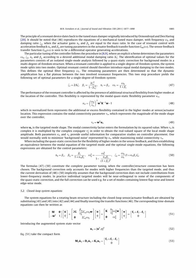
The principle of a resonant device dates back to the tunedmass damper originally introducedbyOrmondroyd andDenHartog[20]. It should be noted that (46) reproduces the equations of a mechanical tuned mass damper, with frequency oZ anddamping ratio zZ, when the actuator gains aZ and bZ are equal to the mass ratio. In the case of resonant control withacceleration feedback aZ and bZ are tuning parameters in the actuator feedback transfer functionGqZðoÞ. The sensor feedbacktransfer function GZqðoÞ is seen to be a differential operator generating accelerations.
The particular tuning of the controller follows the procedure in [8,9],where an explicit schemedetermines the parametersoZ, zZ, aZ and bZ according to a desired additional modal damping ratio Dz. The identification of optimal values for theparameters consists of an isolated single-mode analysis followed by a quasi-static correction for background modes in amulti-degree-of-freedom structure.When a resonant controller is applied to a single-degree-of-freedom system, the systemmode splits into two modes. Optimal resonant control should therefore introduce equal modal damping to the two modes.This defines the optimal filter frequency oc . The remaining parameters are then determined so that the dynamicamplification has a flat plateau between the two involved resonance frequencies. This two step procedure yields thefollowing set of optimal parameters for a single-degree-of-freedom system:
zc ¼ 2Dz, bc ¼2z2c
1�2z2c, ac ¼ bc , oc ¼
on
1þbc
(47)
Theperformanceof the resonant controller is affectedby thepresence of additional structural flexibility fromhighermodes atthe location of the controller. This flexibility is represented by the modal quasi-static flexibility parameter kn,
kn ¼ on
nn
� �2
wTK�1w�1 (48)
which in normalized form represents the additional or excess flexibility contained in the higher modes at sensor/actuatorlocation. This expression contains the nodal connectivity parameter nn, which represents the magnitude of the mode shapeover the controller,
nn ¼wTun (49)
where un is the targeted mode shape. The modal connectivity factor enters the formulation by its squared value. When nn iscomplex it is multiplied by the complex conjugate n�n in order to obtain the real-valued square of the local mode shapeamplitude. Both parameters kn and nn provide useful information for comparative studies on controller placement. Onewould normally seek to minimize ‘background noise’ represented by kn while maximizing nodal connectivity nn.
When including the quasi-static correction for the flexibility of highermodes in the sensor feedback, and then establishingan equivalence between the modal equation of the targeted mode and the optimal single-mode equations, the followingexpressions are obtained for the control parameters:
aZ ¼ bc , bZ ¼bc
1þknbc
, o2Z ¼
o2c
1� knbc
ð1þbcÞ2, zZ ¼
oZ
ocð1þknbcÞzc (50)
The formulas (47)–(50) constitute the complete parameter tuning, when the controller/structure connection has beenchosen. The background correction only accounts for modes with higher frequencies than the targeted mode, and thusthe current derivation of (48)–(50) implicitly assumes that the background correction does not include contributions fromlower-frequency modes. In practice individual targeted modes will be near-orthogonal to some of the components ofthe quasi-static correction, and the full correction can be used e.g. for a set of modes containing lowest flap-wise and lowestedge-wise mode.
5.2. Closed-loop system equations
The system equations for a rotating beam structure including the closed-loop sensor/actuator feedback are obtained bysubstituting (43) and (45) into (42) and (44) and finally inserting the transfer functions (46). The corresponding time-domainequations can then be written as
M 0
�wT 1
� � €u
€Z
" #þ
2GbZn2n
2zZoZw
0 2zZoZ
264
375 _u
_Z
" #þ
KaZn2no2
Zw
0 o2Z
264
375 u
Z
" #¼ feþfC�fG
0
� �(51)
Introducing the augmented system state vector
uZ ¼ ½uT,Z�T (52)
Eq. (51) take the compact form
MZ €uZþDZ _uZþKZuZ ¼feþfC�fG
0
� �(53)
M.N. Svendsen et al. / Journal of Sound and Vibration 330 (2011) 1877–1890 1885
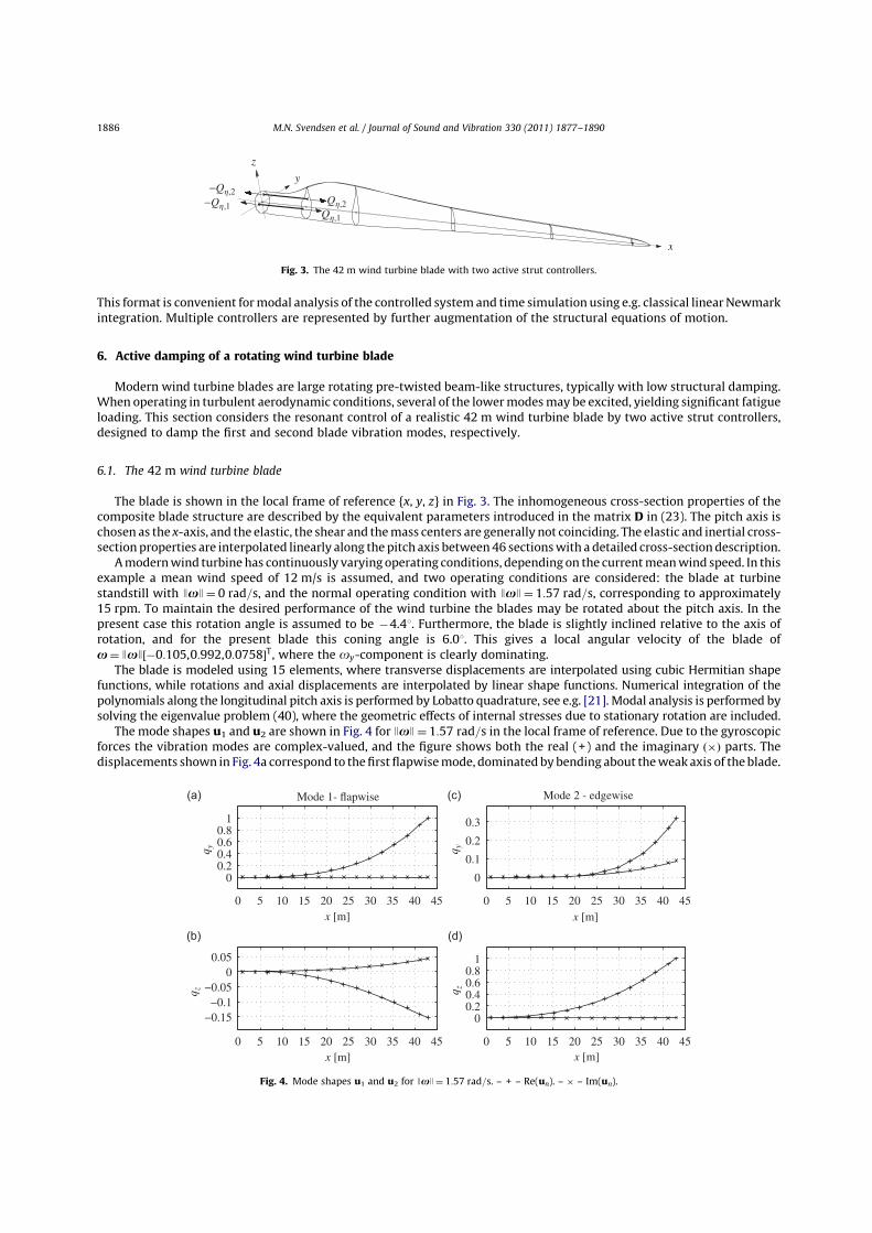
This format is convenient formodal analysis of the controlled system and time simulation using e.g. classical linearNewmarkintegration. Multiple controllers are represented by further augmentation of the structural equations of motion.
6. Active damping of a rotating wind turbine blade
Modern wind turbine blades are large rotating pre-twisted beam-like structures, typically with low structural damping.When operating in turbulent aerodynamic conditions, several of the lowermodesmay be excited, yielding significant fatigueloading. This section considers the resonant control of a realistic 42 m wind turbine blade by two active strut controllers,designed to damp the first and second blade vibration modes, respectively.
6.1. The 42 m wind turbine blade
The blade is shown in the local frame of reference {x, y, z} in Fig. 3. The inhomogeneous cross-section properties of thecomposite blade structure are described by the equivalent parameters introduced in the matrix D in (23). The pitch axis ischosen as the x-axis, and the elastic, the shear and themass centers are generally not coinciding. The elastic and inertial cross-section properties are interpolated linearly along the pitch axis between46 sectionswith a detailed cross-sectiondescription.
Amodernwind turbine has continuously varying operating conditions, depending on the currentmeanwind speed. In thisexample a mean wind speed of 12 m/s is assumed, and two operating conditions are considered: the blade at turbinestandstill with JxJ¼ 0 rad=s, and the normal operating condition with JxJ¼ 1:57 rad=s, corresponding to approximately15 rpm. To maintain the desired performance of the wind turbine the blades may be rotated about the pitch axis. In thepresent case this rotation angle is assumed to be �4.41. Furthermore, the blade is slightly inclined relative to the axis ofrotation, and for the present blade this coning angle is 6.01. This gives a local angular velocity of the blade ofx¼ JxJ½�0:105,0:992,0:0758�T, where the oy-component is clearly dominating.
The blade is modeled using 15 elements, where transverse displacements are interpolated using cubic Hermitian shapefunctions, while rotations and axial displacements are interpolated by linear shape functions. Numerical integration of thepolynomials along the longitudinal pitch axis is performed by Lobatto quadrature, see e.g. [21]. Modal analysis is performed bysolving the eigenvalue problem (40), where the geometric effects of internal stresses due to stationary rotation are included.
The mode shapes u1 and u2 are shown in Fig. 4 for JxJ¼ 1:57 rad=s in the local frame of reference. Due to the gyroscopicforces the vibration modes are complex-valued, and the figure shows both the real (+) and the imaginary ð�Þ parts. Thedisplacements shown in Fig. 4a correspond to thefirst flapwisemode, dominatedbybending about theweak axis of theblade.
x
y
z
Q�,1
−Q�,1Q�,2
−Q�,2
Fig. 3. The 42 m wind turbine blade with two active strut controllers.
0 5 10 15 20 25 30 35 40 45
00.20.40.60.8
1
0 5 10 15 20 25 30 35 40 45
−0.15−0.1
−0.050
0.05
0 5 10 15 20 25 30 35 40 45
0
0.1
0.2
0.3
0 5 10 15 20 25 30 35 40 45
00.20.40.60.8
1
x [m]
x [m]
x [m]
x [m]
q yq z
q yq z
Mode 1- flapwise Mode 2 - edgewise
Fig. 4. Mode shapes u1 and u2 for JxJ¼ 1:57 rad=s. – + – Re(un). – � – Im(un).
M.N. Svendsen et al. / Journal of Sound and Vibration 330 (2011) 1877–18901886
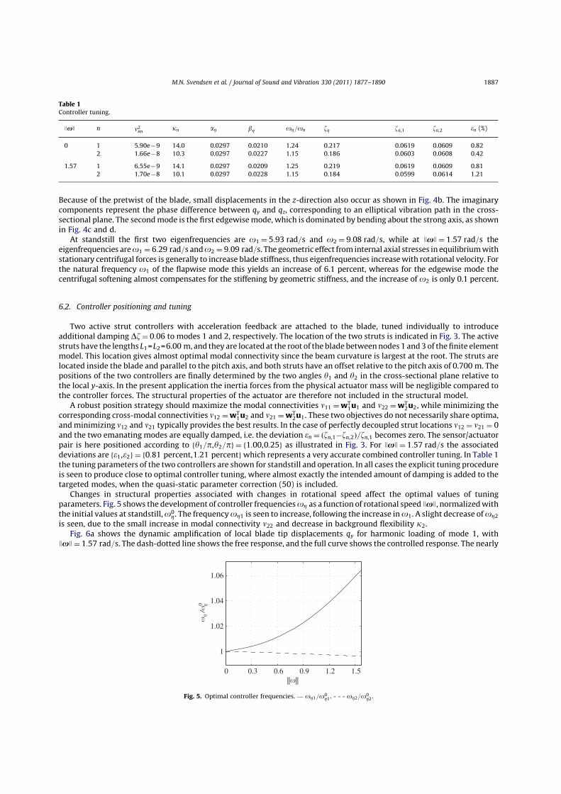
Because of the pretwist of the blade, small displacements in the z-direction also occur as shown in Fig. 4b. The imaginarycomponents represent the phase difference between qy and qz, corresponding to an elliptical vibration path in the cross-sectional plane. The secondmode is the first edgewisemode, which is dominated by bending about the strong axis, as shownin Fig. 4c and d.
At standstill the first two eigenfrequencies are o1 ¼ 5:93 rad=s and o2 ¼ 9:08 rad=s, while at JxJ¼ 1:57 rad=s theeigenfrequencies areo1 ¼ 6:29 rad=s ando2 ¼ 9:09 rad=s. The geometric effect from internal axial stresses in equilibriumwithstationary centrifugal forces is generally to increase blade stiffness, thus eigenfrequencies increasewith rotational velocity. Forthe natural frequency o1 of the flapwise mode this yields an increase of 6.1 percent, whereas for the edgewise mode thecentrifugal softening almost compensates for the stiffening by geometric stiffness, and the increase of o2 is only 0.1 percent.
6.2. Controller positioning and tuning
Two active strut controllers with acceleration feedback are attached to the blade, tuned individually to introduceadditional damping Dz¼ 0:06 to modes 1 and 2, respectively. The location of the two struts is indicated in Fig. 3. The activestruts have the lengths L1=L2=6.00 m, and they are located at the root of the blade betweennodes 1 and3of thefinite elementmodel. This location gives almost optimal modal connectivity since the beam curvature is largest at the root. The struts arelocated inside the blade and parallel to the pitch axis, and both struts have an offset relative to the pitch axis of 0.700 m. Thepositions of the two controllers are finally determined by the two angles y1 and y2 in the cross-sectional plane relative tothe local y-axis. In the present application the inertia forces from the physical actuator mass will be negligible compared tothe controller forces. The structural properties of the actuator are therefore not included in the structural model.
A robust position strategy should maximize the modal connectivities n11 ¼wT1u1 and n22 ¼wT
2u2, while minimizing thecorresponding cross-modal connectivities n12 ¼wT
1u2 and n21 ¼wT2u1. These two objectives do not necessarily share optima,
andminimizing n12 and n21 typically provides the best results. In the case of perfectly decoupled strut locations n12 ¼ n21 ¼ 0and the two emanating modes are equally damped, i.e. the deviation en ¼ ðzn,1�zn,2Þ=zn,1 becomes zero. The sensor/actuatorpair is here positioned according to fy1=p,y2=pg ¼ f1:00,0:25g as illustrated in Fig. 3. For JxJ¼ 1:57 rad=s the associateddeviations are fe1,e2g ¼ f0:81 percent,1:21 percentgwhich represents a very accurate combined controller tuning. In Table 1the tuning parameters of the two controllers are shown for standstill and operation. In all cases the explicit tuning procedureis seen to produce close to optimal controller tuning, where almost exactly the intended amount of damping is added to thetargeted modes, when the quasi-static parameter correction (50) is included.
Changes in structural properties associated with changes in rotational speed affect the optimal values of tuningparameters. Fig. 5 shows the development of controller frequenciesoZ as a function of rotational speed JxJ, normalizedwiththe initial values at standstill,o0
Z. The frequencyoZ1 is seen to increase, following the increase ino1. A slight decrease ofoZ2is seen, due to the small increase in modal connectivity n22 and decrease in background flexibility k2.
Fig. 6a shows the dynamic amplification of local blade tip displacements qy for harmonic loading of mode 1, withJxJ¼ 1:57 rad=s. The dash-dotted line shows the free response, and the full curve shows the controlled response. The nearly
Table 1Controller tuning.
JxJ n n2nn kn aZ bZ oZ=on zZ zn,1 zn,2 en (%)
0 1 5.90e�9 14.0 0.0297 0.0210 1.24 0.217 0.0619 0.0609 0.82
2 1.66e�8 10.3 0.0297 0.0227 1.15 0.186 0.0603 0.0608 0.42
1.57 1 6.55e�9 14.1 0.0297 0.0209 1.25 0.219 0.0619 0.0609 0.81
2 1.70e�8 10.1 0.0297 0.0228 1.15 0.184 0.0599 0.0614 1.21
0 0.3 0.6 0.9 1.2 1.5
1
1.02
1.04
1.06
||�||
��
/�0 �
Fig. 5. Optimal controller frequencies. — oZ1=o0Z1. - - - oZ2=o0
Z2.
M.N. Svendsen et al. / Journal of Sound and Vibration 330 (2011) 1877–1890 1887

symmetrical ‘shoulders’ of the full curve illustrates the almost optimal tuning of the controller. The dashed curve representsthe dynamic amplification for a damped systemwhere the correction for backgroundmodal flexibility is omitted, i.e.k1 ¼ 0. Itis seen that the damping performance of the controller in this case is lost, which illustrates the importance of the quasi-staticcorrection. Fig. 6b shows the dynamic amplification of the local tip displacement qz at harmonic loading of mode 2, and theresults are similar to those in Fig. 6a for mode 1.
The relatively high value k1 ¼ 14:1 corresponds to a significant presence of higher modes at the location of controller 1.This entails some spill-over to these modes, and the added damping to the following two flapwise modes with deflection inthe y-direction is fz5,z7g ¼ f0:0159,0:0232g. With k2 ¼ 10:1 for controller 2 the spill-over to higher modes is somewhatsmaller. The added damping to the following higher modes in the z-direction are fz6,z8g ¼ f0:0058,0:0052g. It is seen thatlimited spill-over can be attained when modal background interference is limited. The general implication is that whenmentionable spill-over is inevitable, it always provides positive contributions. A rigorous proof of the latter has not beenfound, however it is likely to exist due to the collocated nature of the design.
6.3. Simulated structural response
To demonstrate the controller performances in a realistic setting, free and controlled structural response is simulated for aturbulent wind field with realistic stochastic properties. The wind is simulated as a discrete, unidirectional velocity field,where the spatial correlation is established via a Karhunen–Loeve expansion based on independent temporal processes.
The equations of motion (53) are solved using the Newmark integration method with the unconditionally stable ‘averageacceleration’ schemewith parameters g¼ 1
2 and b¼ 14, see e.g. [19]. The geometric stiffnessKg is updated between time instances
ina single-stepprocedure,where the section forces fromthemost recent equilibriumstate areused to computeKg. For small time-steps h relative to the period of the highest important vibration mode Tn this approximation is sufficiently accurate, and in thepresent case T6/h=10. A small amount of algorithmic a-damping with a¼ 0:04 is included to model light structural damping.
In Fig. 7a the local blade tip response qy is shown,where the free response is shownby the dashed curve and the controlledresponse is shown by the full curve. The free response has a quasi-static ‘mean’ component following the resulting blade liftforce, superimposed by oscillations at the natural frequency o1. In the controlled case the oscillations at o1 are seen to besignificantly reduced by the controller, while the ‘mean’ response remains unaffected. Similarly, free and controlled blade tip
0.7 0.8 0.9 1 1.1 1.2 1.30
2
4
6
8
10
12
0.7 0.8 0.9 1 1.1 1.2 1.30
2
4
6
8
10
12
�/�1 �/�2
||qy/
q y||
||qz/
q z||
Fig. 6. Dynamic amplification: (a) Flapwise tip displacement Jqy=qyJ and (b) Edgewise tip displacement Jqz=qzJ. - � - � - Free. — Controlled. - - - kn ¼ 0.
54 56 58 60
1
1.5
2
2.5
3
3.5
4
54 56 58 60
−0.6
−0.4
−0.2
0
t [s]t [s]
q y[m
]
q z[m
]
Fig. 7. Simulated displacement response at blade tip: (a) Flapwise displacements qy and (b) Edgewise displacements qz.
M.N. Svendsen et al. / Journal of Sound and Vibration 330 (2011) 1877–18901888
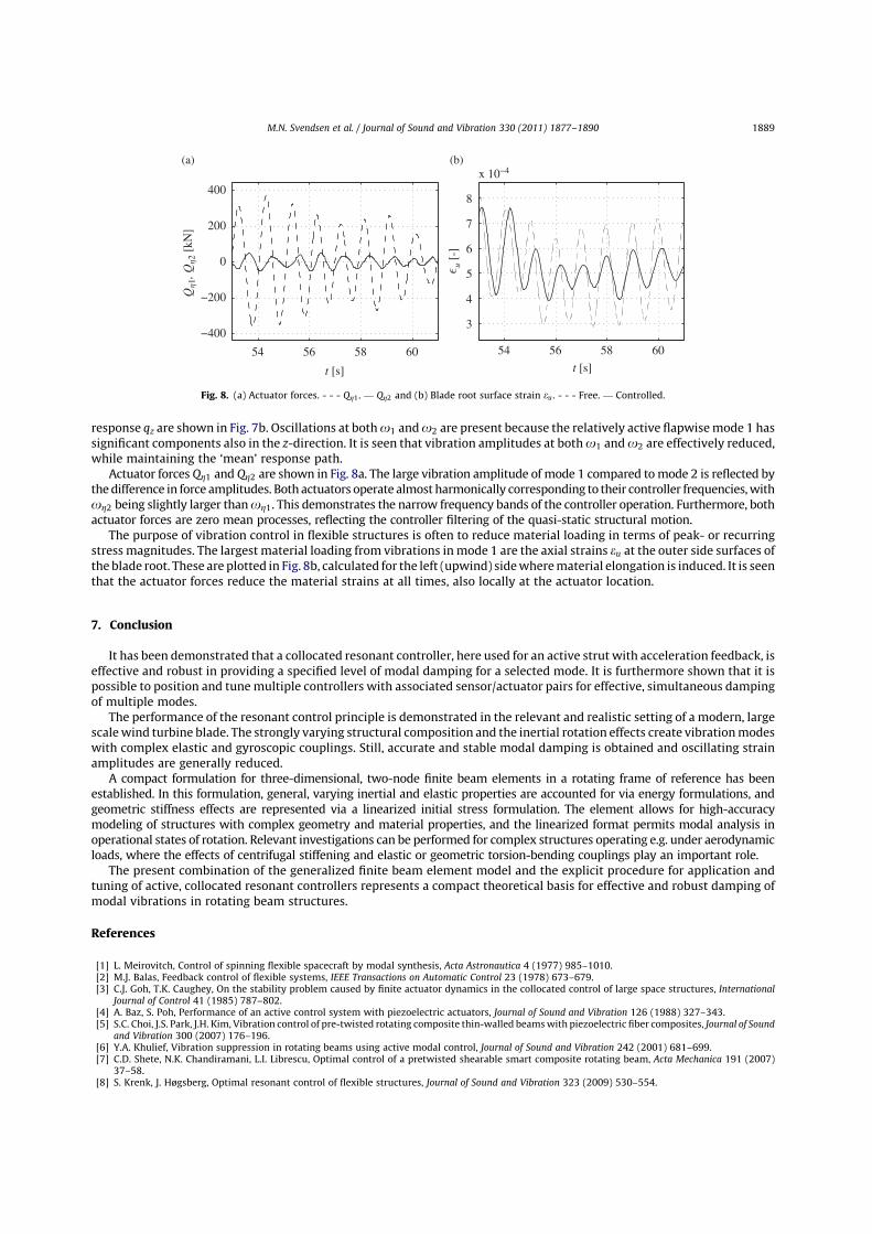
response qz are shown in Fig. 7b. Oscillations at botho1 ando2 are present because the relatively active flapwisemode 1 hassignificant components also in the z-direction. It is seen that vibration amplitudes at botho1 ando2 are effectively reduced,while maintaining the ‘mean’ response path.
Actuator forces QZ1 and QZ2 are shown in Fig. 8a. The large vibration amplitude of mode 1 compared tomode 2 is reflected bythedifference in force amplitudes. Both actuators operate almost harmonically corresponding to their controller frequencies,withoZ2 being slightly larger thanoZ1. This demonstrates the narrow frequency bands of the controller operation. Furthermore, bothactuator forces are zero mean processes, reflecting the controller filtering of the quasi-static structural motion.
The purpose of vibration control in flexible structures is often to reduce material loading in terms of peak- or recurringstress magnitudes. The largest material loading from vibrations inmode 1 are the axial strains eu at the outer side surfaces ofthe blade root. These are plotted in Fig. 8b, calculated for the left (upwind) sidewherematerial elongation is induced. It is seenthat the actuator forces reduce the material strains at all times, also locally at the actuator location.
7. Conclusion
It has been demonstrated that a collocated resonant controller, here used for an active strut with acceleration feedback, iseffective and robust in providing a specified level of modal damping for a selected mode. It is furthermore shown that it ispossible to position and tunemultiple controllers with associated sensor/actuator pairs for effective, simultaneous dampingof multiple modes.
The performance of the resonant control principle is demonstrated in the relevant and realistic setting of a modern, largescalewind turbine blade. The strongly varying structural composition and the inertial rotation effects create vibrationmodeswith complex elastic and gyroscopic couplings. Still, accurate and stable modal damping is obtained and oscillating strainamplitudes are generally reduced.
A compact formulation for three-dimensional, two-node finite beam elements in a rotating frame of reference has beenestablished. In this formulation, general, varying inertial and elastic properties are accounted for via energy formulations, andgeometric stiffness effects are represented via a linearized initial stress formulation. The element allows for high-accuracymodeling of structures with complex geometry and material properties, and the linearized format permits modal analysis inoperational states of rotation. Relevant investigations can be performed for complex structures operating e.g. under aerodynamicloads, where the effects of centrifugal stiffening and elastic or geometric torsion-bending couplings play an important role.
The present combination of the generalized finite beam element model and the explicit procedure for application andtuning of active, collocated resonant controllers represents a compact theoretical basis for effective and robust damping ofmodal vibrations in rotating beam structures.
References
[1] L. Meirovitch, Control of spinning flexible spacecraft by modal synthesis, Acta Astronautica 4 (1977) 985–1010.[2] M.J. Balas, Feedback control of flexible systems, IEEE Transactions on Automatic Control 23 (1978) 673–679.[3] C.J. Goh, T.K. Caughey, On the stability problem caused by finite actuator dynamics in the collocated control of large space structures, International
Journal of Control 41 (1985) 787–802.[4] A. Baz, S. Poh, Performance of an active control system with piezoelectric actuators, Journal of Sound and Vibration 126 (1988) 327–343.[5] S.C. Choi, J.S. Park, J.H. Kim, Vibration control of pre-twisted rotating composite thin-walled beamswith piezoelectric fiber composites, Journal of Sound
and Vibration 300 (2007) 176–196.[6] Y.A. Khulief, Vibration suppression in rotating beams using active modal control, Journal of Sound and Vibration 242 (2001) 681–699.[7] C.D. Shete, N.K. Chandiramani, L.I. Librescu, Optimal control of a pretwisted shearable smart composite rotating beam, Acta Mechanica 191 (2007)
37–58.[8] S. Krenk, J. Høgsberg, Optimal resonant control of flexible structures, Journal of Sound and Vibration 323 (2009) 530–554.
54 56 58 60
−400
−200
0
200
400
54 56 58 60
3
4
5
6
7
8
x 10−4
t [s]t [s]
Q�1
, Q�2
[kN
]
u[-
]
Fig. 8. (a) Actuator forces. - - - QZ1. — QZ2 and (b) Blade root surface strain eu . - - - Free. — Controlled.
M.N. Svendsen et al. / Journal of Sound and Vibration 330 (2011) 1877–1890 1889

[9] S. Krenk, J. Høgsberg, Resonant damping of flexible structures, COMPDYN 2009, ECCOMAS Thematic Conference on Computational Methods in StructuralDynamics and Earthquake Engineering, 2009.
[10] A. Preumont, B. de Marneffe, A. Deraemaeker, F. Bossens, The damping of a truss structure with a piezoelectric transducer, Computers and Structures86 (2008) 227–239.
[11] S. Krenk, Element Stiffness Matrix for Beams with General Cross-section Properties, Technical University of Denmark, Department of MechanicalEngineering, 2006.
[12] K. Washizu, Variational Methods in Elasticity and Plasticity, Pergamon Press, Oxford, 1968.[13] S. Krenk, Lectures on Thin-Walled Beams, third ed., Technical University of Denmark, Department of Mechanical Engineering, 2001.[14] A. Kawamoto, S. Krenk, A. Suzuki, M. Inagaki, Flexible body dynamics in a local frame with explicitly predicted motion, International Journal for
Numerical Methods in Engineering 81 (2010) 246–268.[15] J.H. Argyris, An excursion into large rotations, Computer Methods in Applied Mechanics and Engineering 32 (1982) 85–155.[16] D.H. Hodges, A.R. Atilgan, C.E.S. Cesnik, On a simplified strain energy function for geometrically nonlinear behaviour of anisotropic beams, Composites
Engineering 2 (1992) 513–526.[17] V.Z. Vlasov, Thinwalled Elastic Beams, Israel Program for Scientific Translations, Jerusalem, 1961.[18] L. Meirovitch, A new method of solution of the eigenvalue problem for gyroscopic systems, AIAA Journal 12 (1974) 1337–1342.[19] M. Geradin, D. Rixen, Mechanical Vibrations, second ed., Wiley, Chichester, 1997.[20] J. Ormondroyd, J.P. Den Hartog, The theory of the dynamic vibration absorber, Transactions of the ASME 50 (1928) 9–22.[21] T.J.R. Hughes, The Finite Element Method, Linear Static and Dynamic Finite Element Analysis, Dover, Mineola, New York, 2000.
M.N. Svendsen et al. / Journal of Sound and Vibration 330 (2011) 1877–18901890

P2
(Conference paper)
Resonant vibration control of wind turbine blades
TORQUE 2010: The Science of Making Torque from WindJune 28–30, Creete, Greece, 2010, 543–553


Resonant Vibration Control of Wind Turbine Blades
Martin Nymann Svendsena,b Steen Krenka Jan Høgsberga
[email protected] [email protected] [email protected]
Department of Mechanical Engineeringa,
Technical University of Denmark, DK-2800 Lyngby, Denmark
Vestas Wind Systems A/Sb
Hedeager 42, DK-8200 Aarhus N, Denmark
AbstractThe paper deals with introduction of damp-ing to specific vibration modes of wind turbineblades, using a resonant controller with acceler-ation feedback. The wind turbine blade is rep-resented by three-dimensional, two-node finiteelements in a local, rotating frame of reference.The element formulation accounts for arbitrarymass density distributions, general elastic cross-section properties and geometric stiffness effectsdue to internal stresses. A compact, linear for-mulation for aerodynamic forces with associatedstiffness and damping terms is established andadded to the structural model. The efficiencyof the resonant controller is demonstrated for arepresentative turbine blade exposed to turbu-lent wind loading. It is found that the presentexplicit tuning procedure yields close to optimaltuning, with very limited modal spill-over andeffective reduction of the vibration amplitudes.
Keywords: Resonant control, rotating beam el-ements, aeroelastic beam elements, edgewisedamping.
1 IntroductionVibrations in rotating or idling wind turbineblades is a common phenomenon due to therelatively large and slender proportions of mod-ern blades. Flapwise vibration modes are typi-cally well-damped by aerodynamic forces, whileedgewise vibration modes may have low aerody-namic damping ratios. Therefore, the presentpaper considers introduction of damping to spe-cific edgewise vibration modes in the wind tur-bine blade, using an active collocated resonantcontrol strategy.
The present work adopts a recently devel-oped design procedure for resonant control sys-tems, [1, 2]. The controller is governed by a setof second-order filters with either displacementor acceleration sensor feedback. The controlleris assumed to be collocated, i.e. sensors and
actuators are assumed to operate in pairs withshared physical points of attachment. Actua-tor feedback can e.g. take the form of forces,applied either from an external source at a sin-gle discrete point or from internal devices withtwo distinct attachment points. An example ofan internal device is the active strut, which isa one-dimensional device capable of generatingan axial force [3]. When attached between twocross-sections of e.g. a wind turbine blade, asillustrated in Fig. 1, local bending moments canbe applied to extract energy from edgewise bladevibrations.In the adopted scheme [1,2] the controller pa-
rameters are tuned according to the observationthat optimal damping of the targeted mode isestablished for equal damping of the two closelyspaced modes that replace the original modewhen the controller is introduced into the sys-tem. An explicit quasi-static correction of con-troller parameters accounts for the additionalflexibility from the higher modes of the struc-ture.A compact formulation for three-dimensional,
two-node finite beam elements in a rotatingframe of reference is adopted [4]. In this for-mulation general inertial and elastic propertiesof the beam can be accounted for through theformulation of kinetic and complementary elas-tic energy [5]. Furthermore, geometric stiffnesseffects are introduced by a linearized initial stressformulation [6].In order to investigate the controller perfor-
mance on an aeroelastic wind turbine blade, theaerodynamic forces on the beam elements areintroduced in a state-proportional format. Theformulation is based on the relative inflow an-gles [7, 8], and varying locations of the aero-dynamic centers and the shear center are ac-counted for. The resulting aeroelastic modelallows for direct finite element-based eigensolu-tion analysis and time simulation of the rotatingaeroelastic beam structure.The performance of the resonant controller is
TORQUE 2010: The Science of Making Torque from Wind, June 28-30, Crete, Greece 543

x
yz
Qη
−Qη
Figure 1: An active strut applied to a wind turbine blade.
finally demonstrated in terms of a 42m windturbine blade, where the aim is to provide adesired level of additional damping of the firstedgewise vibration mode. The example bladeincorporates representative structural and aero-dynamic properties of a MW turbine blade butis modelled with a reduced structural dampingin order to better illustrate the qualities of theresonant control. The active device is an activestrut with acceleration feedback. The actuatoris located at the root of the blade where the con-trollability of the critical mode is large, and it isdemonstrated that the properly tuned controlleryields a significant reduction of the edgewise vi-brations of the blade for realistic turbulent windloading.
2 Rotating beam elementThe turbine blade is modeled by three-dimensional two-node finite beam elements ina rotating frame of reference [4]. The framerotates about its origin described by the angu-lar velocity vector ωT = [ωx, ωy, ωz ] and theassociated angular acceleration α = ω. Cross-sections remain planar and the kinematics of thebeam are described through the cross-sectiondisplacements qT = [ qx, qy, qz ] and rotationsrT = [ rx, ry, rz ] with respect to the elementreference axes {x, y, z}. In the present formu-lation the pitch axis of the blade defines thelongitudinal axis x, as shown in Fig. 1. Nodalvalues of the cross-section displacements androtations are organized in the vector uT =[qT
a , rTa , q
Tb , r
Tb ], where subscripts a and b de-
note the two element nodes. Substitution ofkinetic and elastic energy into Lagrange’s equa-tions leads to the following format of the elementequations of motion,
Mu+ 2Gu+Ku = fe + fC − fG (1)
whereM is the mass matrix associated with mo-tion in the local frame of reference, fe is the ex-ternal force vector, G(ω) is the skew-symmetricgyroscopic coupling matrix, fC(ω) is the cen-trifugal force and fG(α) is the angular accelera-tion force. The stiffness matrix K is given as
K = Ke +Kg + G−C (2)
The elastic stiffness matrix Ke is derived froma formulation of the complementary elastic en-ergy [5], accounting for lengthwise variation ofelastic properties of the cross-sections. The cen-trifugal stiffness effect is contained in the sym-metric matrix C(ω), and implies apparent soft-ening of the beam. This softening is balancedby the corresponding geometric stiffening of thebeam, represented in (2) by the geometric stiff-ness matrix Kg(σ). In the present case thegeometric stiffness matrix Kg follows from aformulation of the potential energy associatedwith an initial stress state σ0 [6]. This formu-lation is based on an initial stress field σ = σ0
in the undeformed beam. Hereby the associ-ated geometric stiffness matrix becomes con-stant, once the initial stresses have been de-termined. In the present case this assumptionis relaxed by replacing the initial stresses withthe stresses obtained from an equilibrium stateat current time. In time simulations the equilib-rium state can be established based on the inter-nal stresses from the previous time step, or by afew iteration loops within the present time step.The internal stress state is expressed by the sec-tion forces QT = [Qx, Qy, Qz ] and momentsMT = [Mx, My, Mz ], which are contained inthe element vector fTr = [QT
a , MTa , Q
Tb , M
Tb ],
and the section forces can then be determinedvia the equilibrium equation on element level as
fr = Mu+ 2Gu+Ku− (fe + fC − fG) (3)
The section forces Q and moments M are ener-getically conjugate to the displacements q andthe rotations r. Internal axial forces Qx dueto the centrifugal forces fC generate the well-known centrifugal stiffening effect, while inter-nal shear forces Qy, Qz and bending momentsMy, Mz generate bending/torsion couplings.For stationary rotation with α = 0 the sys-
tem matrices of (1) are constant. If the effectof the centrifugal force is included only in termsof the resulting initial stresses, the homogeneouspart of (1) describes a linear system with nat-ural eigenfrequencies and associated eigenvec-tors. For a rotor system with cantilever blades,K and M are symmetric and positive definite,while G is skew-symmetric. In a state-space for-mulation this leads to purely imaginary eigenval-
TORQUE 2010: The Science of Making Torque from Wind, June 28-30, Crete, Greece 544

ues, appearing in conjugate pairs with associatedcomplex-valued eigenmodes [9].
3 Aerodynamic effectsIn this section a formulation for the state-proportional aerodynamic forces is developed. Aconstant aerodynamic forcing term fa arises cor-responding to the undeformed structural geom-etry, while a stiffness term Kau and a damp-ing term Dau arise from deformation-inducedchanges in inflow angle.
3.1 Angle of attack
Figure 2 illustrates a typical operational positionof a wind turbine profile. The profile is shownwith a combined pitch and twist angle β in thepositive direction, and a direction of the relativewind flow speed W corresponding to a positiveflow angle αW . The profile chord is indicated bythe dotted line.
y
z
WWz
Wy
WD
D
A
HqD
β
Figure 2: Airfoil and flow velocities.
Aerodynamic lift is assumed to be proportionalto the inflow angle α, defined as
α = αf + αK + αD (4)
where αf is the inflow angle component in theundeformed position of the aerodynamic profile,αK is the inflow angle component due to twistof the profile and αD is the relative inflow an-gle component due to the transverse velocity ofthe profile. The spatial position of the profile isexpressed by xT = [x, y, z ], which defines theprofile intersection with the element referenceaxis.The mean wind flow angle αW is given by the
relationtanαW = Wy/Wz (5)
where Wy is the atmospheric wind speed in they-direction and Wz = ‖ω × x‖ is the profile
velocity due to the angular blade velocity. Themean inflow angle αf may then be written as
αf = αW − β + α0 (6)
where α0 represents a constant lift contributiondue to profile camber.The inflow angle component due to cross-
section torsion αK is written as
αK = rx (7)
where rx is the torsional degree of freedom. Thispart of the aerodynamic inflow angle is propor-tional to the state deformation and therefore re-sults in an aerodynamic stiffness term.The last term of (4) is based on the relative in-
flow angle generated by the characteristic profilevelocity qD, perpendicular to the chord as shownin Fig. 2. For airfoils with rotational oscillations,qD is measured at the rear aerodynamic centerH , located on the chord one quarter of the chordlength from the trailing edge [10]. This leads tothe following expression for qD,
qD = qz sinβ − qy cosβ + rxh (8)
where h is the chordwise distance betweenthe shear center A with coordinates aT =[ ax, ay, az ] and the rear aerodynamic center Hwith coordinates hT = [hx, hy, hz ],
h = ‖h‖ − hTa
‖h‖ (9)
The shear center is defined as the point in across-section where a shear force will not intro-duce torsion. The cross-section rotates aboutthe shear center when subjected to a torsionalmoment.The relative inflow angle component αD can
be determined from the relation sinαD =qD/WD, where
WD = W cos(αW − β) (10)
is the flow speed parallel to the chord. For smallangles, i.e. qD � WD, the following approxi-mation can be made,
αD � 1
WD
(
qz sinβ − qy cosβ + rxh) (11)
Substitution of (6), (7) and (11) into (4) givesthe following expression for the inflow angle α,
α = αW + β + α0 + rx
+1
WD
(
qz sinβ − qy cosβ + rxh)(12)
The last part of the aerodynamic inflow angle isproportional to the velocity states, hence repre-senting aerodynamic damping.
TORQUE 2010: The Science of Making Torque from Wind, June 28-30, Crete, Greece 545

3.2 Aerodynamic element forcesThe aerodynamic pressure distribution is as-sumed to correspond to a resulting lift force FL,perpendicular to the flow angle αW , and a re-sulting drag force FD, parallel to the flow an-gle αW . The two forces are assumed to actthrough the aerodynamic center D with coordi-nates dT = [ dx, dy, dz ]. For a thin flat platethe aerodynamic center is located one quarterof the plate width from the leading edge. Theaerodynamic forces FL and FD are organized inthe vector FW and given as
FW =
[
FL
FD
]
= 12�aCW 2α
[
C′
L
C′
D
]
(13)
where �a is the air mass density, C is the chordlength, and C′
L, C′
D are lift and drag curve in-clinations. The wind velocity W relative to theaerodynamic profile is given as
W =√
W 2y +W 2
z (14)
By insertion of (12) into (13) the following ex-pression for FW can be written,
FW = F+AK
[
qr
]
+AD
[
qr
]
(15)
where the matrices AK and AD are given inAppendix A. Aerodynamic forces Qa and mo-ments Ma acting at the element reference axisare written as
[
Qa
Ma
]
= TRFW (16)
Here R is a transformation matrix for rotationof FW into equivalent forces in D aligned withthe element coordinate system, and T is a trans-formation matrix that establishes the equivalentforces and moments at the reference axis. Thematrices R and T are given in Appendix A.Element nodal forces and moments are ob-
tained by the virtual work δV expressed in termsof the conjugate virtual displacements δq androtations δr,
δV =
∫
L
[
δqT , δrT]T
[
Qa
Ma
]
dx (17)
The displacement field is interpolated via nodaldegrees of freedom u and shape functionsN(x),such that
[
qr
]
= N(x)u (18)
Inserting (18) into (17) leads to the followingexpression for the virtual work,
δV = δuT
∫
L
NT
[
Qa
Ma
]
dx (19)
Substitution of (15) into (16), followed by sub-stitution into (19) implies that the virtual workby the external load can be written as δV =δuT f , whereby the resulting force vector can beidentified as
f = fa +Kau+Dau (20)
where the aerodynamic force vector fa, the aero-dynamic stiffness matrix Ka and the aerody-namic damping matrix Da are given in Ap-pendix A.The aerodynamic stiffness matrix is not nec-
essarily positive definite. Thus, aerodynamicstiffness effects may reduce or increase struc-tural eigenfrequencies. The aerodynamic damp-ing matrix is non-symmetric, and thus the clas-sic modal decoupling via orthogonal eigenmodesdoes not apply directly. This implies that modesmay be energetically coupled, i.e. vibration en-ergy may be transferred between modes. Finally,the damping matrix is not necessarily positivedefinite, which means that the vibration modesmay be negatively damped.
4 Resonant vibration controlIn this section the filters of the resonant con-troller are defined as transfer functions in the fre-quency domain, and the tuning procedure for asystem with acceleration feedback is presented.Details about the tuning procedure are givenin [1, 2].
4.1 Controller formatThe objective of the controller is to extractmodal energy by imposing a specifically tunedresonant force to the structure. Actuator feed-back is represented by the force vector fη, andthe resulting structural equations of motion be-come
Mu+Du+Ku =
fe + fC − fG + fa + fη(21)
The system (21) is the complete representationof the aeroelastic beam, where the system damp-ing matrix D is the sum of the gyroscopic matrixG and the aerodynamic damping matrix Da,
D = 2G−Da (22)
and where the system stiffness matrix K is
K = Ke +Kg + G−C−Ka (23)
The resonant controller is conveniently definedin the frequency domain. The beam is assumedto rotate with constant angular velocity ω, i.e.α = 0 and fG = 0. Deformations due to the
TORQUE 2010: The Science of Making Torque from Wind, June 28-30, Crete, Greece 546
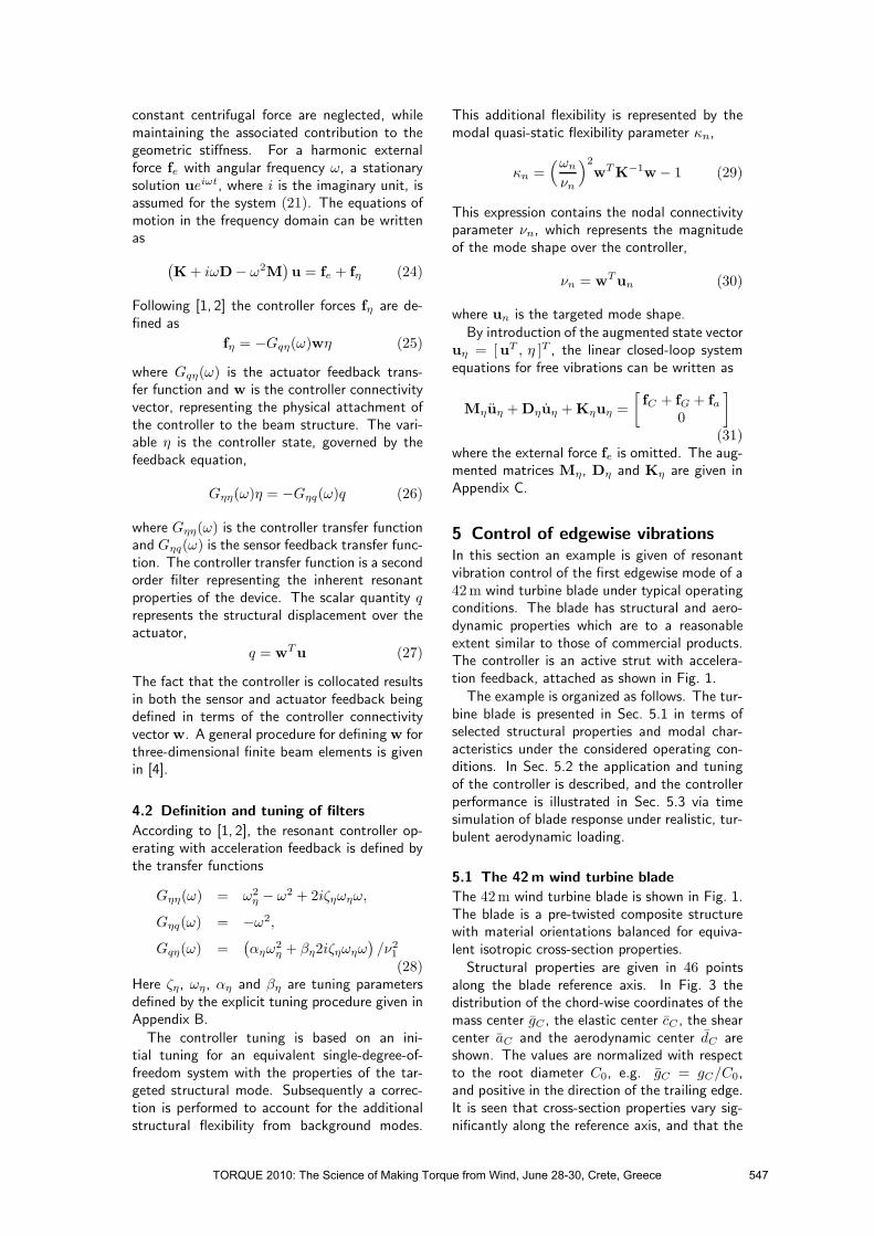
constant centrifugal force are neglected, whilemaintaining the associated contribution to thegeometric stiffness. For a harmonic externalforce fe with angular frequency ω, a stationarysolution ueiωt, where i is the imaginary unit, isassumed for the system (21). The equations ofmotion in the frequency domain can be writtenas
(
K+ iωD− ω2M)
u = fe + fη (24)
Following [1, 2] the controller forces fη are de-fined as
fη = −Gqη(ω)wη (25)
where Gqη(ω) is the actuator feedback trans-fer function and w is the controller connectivityvector, representing the physical attachment ofthe controller to the beam structure. The vari-able η is the controller state, governed by thefeedback equation,
Gηη(ω)η = −Gηq(ω)q (26)
where Gηη(ω) is the controller transfer functionand Gηq(ω) is the sensor feedback transfer func-tion. The controller transfer function is a secondorder filter representing the inherent resonantproperties of the device. The scalar quantity qrepresents the structural displacement over theactuator,
q = wTu (27)
The fact that the controller is collocated resultsin both the sensor and actuator feedback beingdefined in terms of the controller connectivityvectorw. A general procedure for definingw forthree-dimensional finite beam elements is givenin [4].
4.2 Definition and tuning of filters
According to [1, 2], the resonant controller op-erating with acceleration feedback is defined bythe transfer functions
Gηη(ω) = ω2η − ω2 + 2iζηωηω,
Gηq(ω) = −ω2,
Gqη(ω) =(
αηω2η + βη2iζηωηω
)
/ν21(28)
Here ζη, ωη, αη and βη are tuning parametersdefined by the explicit tuning procedure given inAppendix B.
The controller tuning is based on an ini-tial tuning for an equivalent single-degree-of-freedom system with the properties of the tar-geted structural mode. Subsequently a correc-tion is performed to account for the additionalstructural flexibility from background modes.
This additional flexibility is represented by themodal quasi-static flexibility parameter κn,
κn =(ωn
νn
)2
wTK−1w− 1 (29)
This expression contains the nodal connectivityparameter νn, which represents the magnitudeof the mode shape over the controller,
νn = wTun (30)
where un is the targeted mode shape.By introduction of the augmented state vector
uη = [uT , η ]T , the linear closed-loop systemequations for free vibrations can be written as
Mηuη +Dηuη +Kηuη =
[
fC + fG + fa0
]
(31)where the external force fe is omitted. The aug-mented matrices Mη, Dη and Kη are given inAppendix C.
5 Control of edgewise vibrationsIn this section an example is given of resonantvibration control of the first edgewise mode of a42m wind turbine blade under typical operatingconditions. The blade has structural and aero-dynamic properties which are to a reasonableextent similar to those of commercial products.The controller is an active strut with accelera-tion feedback, attached as shown in Fig. 1.The example is organized as follows. The tur-
bine blade is presented in Sec. 5.1 in terms ofselected structural properties and modal char-acteristics under the considered operating con-ditions. In Sec. 5.2 the application and tuningof the controller is described, and the controllerperformance is illustrated in Sec. 5.3 via timesimulation of blade response under realistic, tur-bulent aerodynamic loading.
5.1 The 42m wind turbine blade
The 42m wind turbine blade is shown in Fig. 1.The blade is a pre-twisted composite structurewith material orientations balanced for equiva-lent isotropic cross-section properties.Structural properties are given in 46 points
along the blade reference axis. In Fig. 3 thedistribution of the chord-wise coordinates of themass center gC , the elastic center cC , the shearcenter aC and the aerodynamic center dC areshown. The values are normalized with respectto the root diameter C0, e.g. gC = gC/C0,and positive in the direction of the trailing edge.It is seen that cross-section properties vary sig-nificantly along the reference axis, and that the
TORQUE 2010: The Science of Making Torque from Wind, June 28-30, Crete, Greece 547

0 5 10 15 20 25 30 35 40 45
0.2
0.1
0
0.1
0.2 gC
cCaC
dC
x [ m ]
g C,c C
,aC,dC
Figure 3: Characteristic coordinates.
mass center, the shear center and the aerody-namic center are generally not coinciding.The modal characteristics of the blade are de-
termined for the stationary operating conditionswith Wy = 12m/s, ||ω|| = 1.57 rad/s corre-sponding to 15 rpm, and βp = 4.4◦. The bladehas a coning angle of γ = 6.0◦ relative to therotor plane.The blade is modeled using 15 elements,
whereby each element spans approximately threedata points, of which two are located at the el-ement ends. Cross-section properties are inter-polated linearly between data points. Hermi-tian shape functions are used for interpolationof transverse displacements and linear functionsare used for interpolation of axial displacementsand rotations. The integrals (A.5) are evaluatednumerically by Lobatto quadrature [11], whichtakes end-point values into account.Geometric stiffness effects are determined ac-
cording to the section forces and moments in-troduced by centrifugal and aerodynamic forces.Centrifugal forces lead to internal axial forces,which generate a stiffening of the blade. Aero-dynamic forces lead to internal shear forces andbending moments, by which bending/torsioncouplings arise. The eigenfrequency of flapwisemodes is generally increased due to the geomet-ric stiffening, whereas this effect is to a largeextent counteracted by centrifugal softening inthe case of edgewise modes.Due to the aerodynamic damping term, rela-
tively large damping ratios are found for flapwisemodes, e.g. ζ1 = 0.462 and ζ3 = 0.164 for thefirst two, while relatively low damping values arefound for the edgewise modes, e.g. ζ2 = 0.007and ζ4 = 0.001 for the first two. In practice,edgewise damping ratios are somewhat higherdue to e.g. intrinsic material damping, not rep-resented here.The first edgewise mode has the eigen-
frequency ω2 = 9.17 rad/s corresponding to1.46Hz, and the mode shape u2 shown in Fig.
4 in terms of local degrees of freedom. The localdegrees of freedom refer to the original elementcoordinate system as shown in Fig. 1, which fol-lows the elements through rotation according tothe pitch and coning angles. The mode is nor-malized such that the largest real part of thelocal displacement component qz equals 1 inFig. 4a. Here the typical vibration mode of acantilever beam is recognized.
0 5 10 15 20 25 30 35 40 45
00.20.40.60.8
1 Re(uj)Im(uj)
0 5 10 15 20 25 30 35 40 45
00.10.20.30.40.5
0 5 10 15 20 25 30 35 40 45
0.060.040.02
0
x [ m ]
x [ m ]
x [ m ]
q zq y
r x
Figure 4: Mode shape u2 for Wy = 12m/s.
In Fig. 4b the flapwise displacement compo-nent qy of u2 is shown. It is seen that both a realpart in phase with qz and an imaginary part witha π/2 phase difference to qz is present. The in-phase part represents an elastic (qy, qz)-couplingdue to the pre-twist of the blade. The part of qywhich is π/2 out of phase with qz is generatedby gyroscopic forces and aerodynamic dampingforces, of which the aerodynamic contribution ispredominant in the present case.
The modal torsional rotation components rxare shown in Fig. 4c. The real components aregenerated by the shear- and mass centers beingnon-coinciding, and this presence of torsion re-sults in aerodynamic stiffening of the vibrationmode. The imaginary components of rx aregenerated by the shear- and aerodynamic cen-ters being non-coinciding, whereby aerodynamicdamping forces induce torsional moments.
TORQUE 2010: The Science of Making Torque from Wind, June 28-30, Crete, Greece 548

5.2 Controller Application and Tuning
The first edgewise vibration mode has beenshown to have a low aerodynamic damping ra-tio. In this section a collocated active strut withacceleration feedback is applied to the turbineblade in order to introduce additional dampinginto this particular mode. The choice of phys-ical placement and the explicit tuning of thecontroller is based on the modal characteristicsshown in the previous section.
The first edgewise vibration is primarily abending mode in the local z-direction, in whichthe largest curvatures occur at the fixed endof the blade. Thus, for optimized modal con-trollability and observability, the active strutis fitted at the blade root with a finite dis-tance in the local z-direction to the elasticcenter. Bending moments can hereby be in-duced to control the dominant components ofthe addressed mode. The attachment pointsare denoted V1 and V2, where V1 is locatedat the root cross-section with local coordinates[ v1x, v
1y , v
1x ] = [ 1.00, 0.05, 0.70 ]m and V2 is
located 6.00m into the blade, i.e. with local co-ordinates [ v2x, v
2y, v
2x ] = [ 7.00, 0.05, 0.70 ]m.
Thus, the length of the active strut is 6.00m.The finite, positive components v1y , v
2y are cho-
sen due to the inclined modal cross-section vi-bration path induced by the components qy ofmode 2.
A few of the higher vibration modes of thefree structure are negatively damped by aerody-namic forces. In order to stabilize these modes intime integration, a moderate amount of Rayleighdamping and algorithmic α-damping is added tothe system. This increases the ‘inherent’ damp-ing ratio of mode 2 in the uncontrolled referencesystem to ζ2 = 0.009.
The controller is tuned according to the modalproperties under the stationary operating con-ditions of Wy = 12m/s, ||ω|| = 1.57 rad/scorresponding to 15 rpm and βp = 4.4◦. Thedesired additional amount of damping is set toΔζ = 0.060. The physical connection of thecontroller defines the modal connectivity param-eter ν2 and the modal quasi-static flexibility pa-rameter κ2, and the controller parameters aresubsequently determined according to the for-mulas (B.1)-(B.4). The resulting values aregiven in Table 1.
When the controller is applied, the targetedmode splits into two new, closely spaced modes.For optimal tuning the two modes have equaldamping ratios ζn,1 and ζn,2. In the presentcase the deviations of ζ2,1 and ζ2,2 from themean value ζ2 = (ζ2,1 + ζ2,2)/2 are ±0.92%.The blade tip displacement frequency responsein the local z-direction according to simultane-
Table 1: Controller parameters.
ζc · 10−1 1.200 βc · 10−2 2.965
ωc 8.902 αc · 10−2 2.965
κ2 7.231 βη · 10−2 2.442
|ν2|2 · 10−8 2.360 αη · 10−2 2.965
ωη 9.967 ζ2,1 · 10−2 6.625
ζη · 10−1 1.632 ζ2,2 · 10−2 6.747
ous unit tip loads in the y- and z-directions isshown in Fig. 5. The two vertical dotted lines in-dicate the eigenfrequencies ω1 and ω2 of the un-controlled system. The uncontrolled frequencyresponse is seen to have a significant resonantpeak at ω2, whereas the controlled system isclearly reduced. The slightly sub-optimal tuningresults in the small lack of symmetry of the twodamped response peaks.
0.6 0.8 1 1.2 1.40
2
4
6
8
10
12 FreeContr.
ω/ω2
q z/q z
Figure 5: Edgewise tip displacement frequencyresponse to flap- and edgewise load.
The present limitation of the controller tun-ing quality is due to the complex structural con-figuration of the turbine blade. The significantblade twist implies that modes generally consistof displacements in both the y- and z-directions.Thus, structural feedback will in principle con-tain unwanted contributions from all structuralmodes. Similarly, controller feedback will, inprinciple, induce a general excitation of struc-tural modes. However, a key property of thecontroller is the very limited amount of modalspill-over. This is due to the narrow, frequency-wise band of actuator forces due to the inherentresonant nature of the controller. Table 2 showsthe first four eigenfrequencies and damping ra-tios of the free and controlled system. A smallamount of spill-over in terms of added dampingis seen to the second edgewise mode (mode 4),while the flapwise modes (modes 1 and 3) arepractically unaffected by the controller.
The mean added damping is ζ2−ζfr2 = 0.058,
TORQUE 2010: The Science of Making Torque from Wind, June 28-30, Crete, Greece 549

Table 2: Eigenfrequencies and damping ratios.
n ζfrn ζctrn ωfrn ωctr
n
1 0.464 0.463 6.12 6.16
2,1 0.009 0.066 9.17 8.38
2,2 - 0.068 - 9.76
3 0.167 0.167 16.6 16.6
4 0.007 0.019 27.7 28.1
which is somewhat smaller than the desiredvalue, Δζ = 0.060. This is due to the factthat the effect of a local damper can not beadded directly for damped structures. An accu-rate formula for the combined effect has beengiven in [12].In the simpler case of prismatic beams with
complex dynamic properties, close to optimaltuning can be obtained [4]. For the present pur-pose the tuning quality is however highly sat-isfactory. This is further demonstrated in thefollowing section.
5.3 Controlled System Response
In the following the controller performance isdemonstrated via time simulation of free andcontrolled blade responses. The blade is sub-jected to a realistic 600 s turbulent wind fieldwith the average wind speed Wy = 12m/s. Fullspatial correlation of wind velocities is assumedfor simplicity.The simulation is performed with prescribed
angular velocity ω and angular acceleration α.A spin-up sequence during the first three sec-onds accelerates the blade from a complete restto the angular velocity ||ω|| = 1.57 rad/s cor-responding to 15 rpm, which is kept constantat this level for the remaining simulation time.The blade pitch is kept constant at βp = 4.4◦,regardless of wind speed fluctuations.In Fig. 6 sequences of the local edgewise blade
tip displacements qz are shown. The time scaleis normalized with the period of mode 2, T2. Inthe free response, significant oscillations at thefrequency of mode 2 are seen. In the controlledresponse these oscillations are reduced, while thequasi-static ‘mean’ vibration path is practicallyunchanged. This demonstrates the frequency-specific targeting of controller forces obtainedin the controller tuning.The local flapwise displacements qy are shown
in Fig. 7. It is seen that the free and controlledresponses are almost identical. This demon-strates the specific kinematic targeting of con-troller forces, achieved by placement of the con-troller such that bending moments are primarilyinduced about the principal axes about which
24 26 28 30 320.64
0.6
0.56
0.52
0.48
FreeControlled
t/T2
q z[m
]
Figure 6: Edgewise tip displacements.
cross-sections rotate to generate displacementsin the z-direction. The blade pre-twist impliesthat the orientation of principal axes varies alongthe beam, and particularly, over the extension ofthe controller.
24 26 28 30 32
3.3
3.45
3.6
3.75 FreeControlled
t/T2
q y[m
]
Figure 7: Flapwise tip displacements.
One objective of actively adding damping toone or more specific modes may be to reducematerial damaging from cyclic loading. Dis-placements generated by mode 2 induce thelargest material strains εu on the surface ofthe blade root, near the intersections betweenthe surface and the local z-axis. In Fig. 8 theroot surface strains εu are plotted. The rootsurface strains are here determined as εu =Qx/A
E + 12szMy/I
Eyy, where AE is the axial
cross-section stiffness, IEyy is the cross-sectionbending stiffness about the y-axis and sz is thedistance from the element reference axis to theintersection between the blade surface and thethe local z-axis in the positive direction.The values of εu are positive, corresponding to
elongation. It is seen that the amplitude of varia-tions in surface strains due to vibrations in mode2 are significantly reduced by the controller. Fur-thermore, the shown strains are determined at aphysical location close to the active device wheresignificant axial control forces Qη are applied.
TORQUE 2010: The Science of Making Torque from Wind, June 28-30, Crete, Greece 550
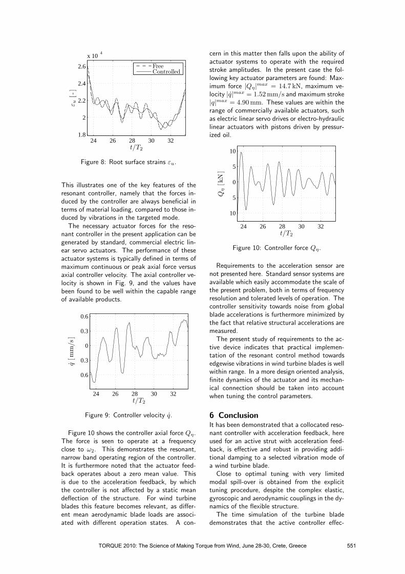
24 26 28 30 321.8
2
2.2
2.4
2.6x 10 4
FreeControlled
t/T2
ε u[-]
Figure 8: Root surface strains εu.
This illustrates one of the key features of theresonant controller, namely that the forces in-duced by the controller are always beneficial interms of material loading, compared to those in-duced by vibrations in the targeted mode.The necessary actuator forces for the reso-
nant controller in the present application can begenerated by standard, commercial electric lin-ear servo actuators. The performance of theseactuator systems is typically defined in terms ofmaximum continuous or peak axial force versusaxial controller velocity. The axial controller ve-locity is shown in Fig. 9, and the values havebeen found to be well within the capable rangeof available products.
24 26 28 30 32
0.6
0.3
0
0.3
0.6
t/T2
q[m
m/s]
Figure 9: Controller velocity q.
Figure 10 shows the controller axial force Qη.The force is seen to operate at a frequencyclose to ω2. This demonstrates the resonant,narrow band operating region of the controller.It is furthermore noted that the actuator feed-back operates about a zero mean value. Thisis due to the acceleration feedback, by whichthe controller is not affected by a static meandeflection of the structure. For wind turbineblades this feature becomes relevant, as differ-ent mean aerodynamic blade loads are associ-ated with different operation states. A con-
cern in this matter then falls upon the ability ofactuator systems to operate with the requiredstroke amplitudes. In the present case the fol-lowing key actuator parameters are found: Max-imum force |Qη|max = 14.7 kN, maximum ve-locity |q|max = 1.52mm/s and maximum stroke|q|max = 4.90mm. These values are within therange of commercially available actuators, suchas electric linear servo drives or electro-hydrauliclinear actuators with pistons driven by pressur-ized oil.
24 26 28 30 32
10
5
0
5
10
t/T2
Qη[kN]
Figure 10: Controller force Qη.
Requirements to the acceleration sensor arenot presented here. Standard sensor systems areavailable which easily accommodate the scale ofthe present problem, both in terms of frequencyresolution and tolerated levels of operation. Thecontroller sensitivity towards noise from globalblade accelerations is furthermore minimized bythe fact that relative structural accelerations aremeasured.The present study of requirements to the ac-
tive device indicates that practical implemen-tation of the resonant control method towardsedgewise vibrations in wind turbine blades is wellwithin range. In a more design oriented analysis,finite dynamics of the actuator and its mechan-ical connection should be taken into accountwhen tuning the control parameters.
6 ConclusionIt has been demonstrated that a collocated reso-nant controller with acceleration feedback, hereused for an active strut with acceleration feed-back, is effective and robust in providing addi-tional damping to a selected vibration mode ofa wind turbine blade.Close to optimal tuning with very limited
modal spill-over is obtained from the explicittuning procedure, despite the complex elastic,gyroscopic and aerodynamic couplings in the dy-namics of the flexible structure.The time simulation of the turbine blade
demonstrates that the active controller effec-
TORQUE 2010: The Science of Making Torque from Wind, June 28-30, Crete, Greece 551

tively reduces the otherwise significant vibrationamplitudes in the targeted edgewise mode, whilebeing always beneficial in terms of material load-ing, both globally and locally.While mode 2 is damped, the remaining vi-
bration modes are practically unaffected. Theinsignificant spill-over demonstrates that con-troller efforts are effectively limited to the in-tended purpose. The found requirements to theactive device indicate that implementation ofthe resonant control method towards edgewisevibrations in wind turbine blades is well withinpractical range.The structural model adopts a formulation
for three-dimensional, two-node finite beam el-ements in a local, rotating frame of reference.The element allows for high-accuracy modelingof structures with arbitrary mass distributions,general elastic properties and geometric stiffnesseffects due to internal stresses. Here a compactformulation for state-proportional aerodynamicforces on the same element type has been es-tablished. In this formulation, varying locationsof the aerodynamic centers and the shear cen-ter are accounted for, and the resulting aerody-namic stiffness and damping terms can be addeddirectly to the structural model. The result-ing model allows for direct, finite element-basedeigensolution analysis and time simulation of ro-tating, aeroelastic beam structures.The present combination of the aeroelastic
blade model with the explicit procedure for appli-cation and tuning of active, collocated resonantcontrollers represents a compact theoretical ba-sis for effective and robust damping of modalvibrations in wind turbine blades.
References[1] S. Krenk, J. Høgsberg, Optimal resonant
control of flexible structures, Journal ofSound and Vibration, 323 (2009) 530–554.
[2] S. Krenk, J. Høgsberg, Resonant damp-ing of flexible structures, COMPDYN 2009,ECCOMAS Thematic Conference on Com-
putational Methods in Structural Dynamics
and Earthquake Engineering (2009).
[3] A. Preumont, B. de Marneffe, A. Derae-maeker, F. Bossens, The damping of a trussstructure with a piezoelectric transducer,Computers & Structures, 86 (2008) 227–239.
[4] M. N. Svendsen, S. Krenk, J. Høgsberg,Resonant vibration control of rotatingbeams, To be published, (2010).
[5] S. Krenk, Element stiffness matrix for
beams with general cross-section prop-
erties, Technical University of Denmark,
Department of Mechanical Engineering,(2006).
[6] S. Krenk, Lectures on thin-walled beams,Technical University of Denmark, Depart-ment of Mechanical Engineering, (2006).
[7] J. W. Larsen, S. R. K. Nielsen, S. Krenk,Dynamic stall model for wind turbine air-foils, Journal of Fluids and Structures, 23(2007) 959–982.
[8] M. H. Hansen, Aeroelastic instability prob-lems for wind turbines, Wind Energy, 10(2007) 551–557.
[9] M. Geradin, D. Rixen, Mechanical Vibra-tions, second ed., Wiley, Chichester, 1997.
[10] Y. C. Fung, An Introduction to the The-
ory of Aeroelasticity, Dover, Mineola, NewYork, 1993.
[11] T. J. R. Hughes, The Finite Element
Method, Linear Static and Dynamic Finite
Element Analysis, Dover, Mineola, NewYork, 2000.
[12] S. Krenk, J. Høgsberg, Tuned mass ab-sorbers on damped structures under ran-dom load, Probabilistic Engineering Me-
chanics, 23 (2008) 408–415.
A Aerodynamic terms
AK = 12�aCW 2
[
0 0 0 C′
L 0 00 0 0 C′
D 0 0
]
(A.1)
AC = 1
2�aC
W2
WD[0 −C′
L cos(β) C′
L sin(β) C′
Lh 0 0
0 −C′
D cos(β) C′
D sin(β) C′
Dh 0 0
]
(A.2)
R =
[
0 0cosαW sinαW
− sinαW cosαW
]
(A.3)
T =
⎡
⎢
⎢
⎢
⎢
⎢
⎣
1 0 00 1 00 0 10 −dz dydz 0 0−dy 0 0
⎤
⎥
⎥
⎥
⎥
⎥
⎦
(A.4)
fa =
∫
L
NTTRFdx,
Ka =
∫
L
NTTRAKdx,
Da =
∫
L
NTTRADdx
(A.5)
TORQUE 2010: The Science of Making Torque from Wind, June 28-30, Crete, Greece 552

B Controller tuning
ζc = 2Δζ, β =2ζ2c
1− 2ζ2c, (B.1)
αη = β, βη =β
1 + κnβ, (B.2)
ω2η =
1
1− κnβ
(1 + β)2
( ωn
1 + β
)2
, (B.3)
ζη =1
ωη (1 + κnβ)
(
1− κnβ
(1 + β)2
)
ζcωn
1 + β
(B.4)
C Closed-loop system matrices
Mη =
[
M 0−wT 1
]
(C.1)
Dη =
⎡
⎣
Dβη
ν2n2ζηw
0 2ζηωη
⎤
⎦ (C.2)
Kη =
[
Kαη
ν2nω2ηw
0 ω2η
]
(C.3)
TORQUE 2010: The Science of Making Torque from Wind, June 28-30, Crete, Greece 553


P3
(Journal paper)
Resonant vibration control of three-bladed wind turbine rotors
SubmittedJanuary 2011


Resonant Vibration Control of Three-Bladed
Wind Turbine Rotors
S. Krenk†, M.N. Svendsen†,‡ and J. Høgsberg†
†Department of Mechanical Engineering,Technical University of Denmark, DK-2800 Lyngby, Denmark
‡Vestas Wind Systems A/S,Hedeager 42, DK-8200 Aarhus N, Denmark
Abstract. Rotors with blades as e.g. in wind turbines are prone to vibrations due to the
flexibility of the blades and the support. In the present paper a theory is developed for active
control of a combined set of vibration modes in three-bladed rotors. The control system consists
of identical collocated actuator-sensor pairs on each of the blades and targets a set of three modes
constituting a collective mode with identical motion of all the blades, and two independent
whirling modes, in which a relative motion pattern moves forward or backward over the rotor.
The natural frequency of the collective mode is typically lower than the frequency of the whirling
modes due to support flexibility. The control signals from the blades are combined into a mean
signal, addressing the collective mode, and three components from which the mean signal has
be subtracted, addressing the pair of whirling modes. The response of the actuators is tuned to
provide resonant damping of the collective mode and the whirling modes by using the separate
resonance characteristics of the collective and the whirling modes. In the calibration of the
control parameters it is important to account for the added flexibility of the structure due
to influence of other non-resonant modes. The efficiency of the method is demonstrated by
application to a rotor with 42 meter blades, where the sensor-actuator system is implemented
in the form of an axial extensible strut near the root of each blade. The load is provided by
a simple but fully three-dimensional correlated wind velocity field. It is shown by numerical
simulations that the active damping system can provide a significant reduction in the response
amplitude of the targeted modes, while applying control moments to the blades that are about
one order of magnitude smaller than the moments from the external load.
Nomenclature
A,B = state-space matricesC = centrifugal stiffness matrixD𝑎 = aerodynamic damping matrixF = state-space forcef = total forcef𝑒 = external forcef𝑐 = centrifugal forcesf𝑔 = gyroscopic forcesf𝜂 = control forceG = gyroscopic stiffness matrix𝑔𝛼, 𝑔𝛽 , 𝑔𝜁, 𝑔𝜔 = effective system control parameters𝐺𝑐(𝜔), 𝐺𝑤(𝜔) = control filter for collective and whirling modes𝑖 = complex imaginary unit
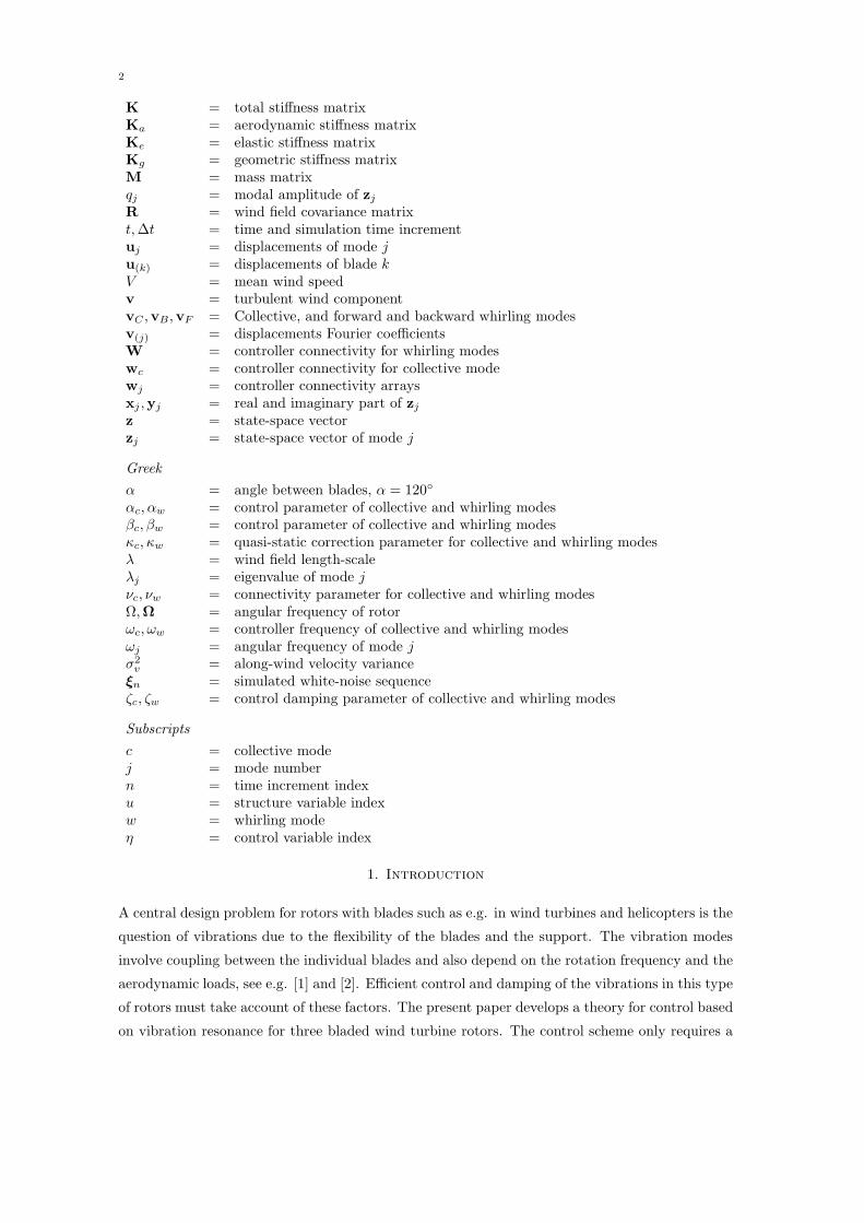
2
K = total stiffness matrixK𝑎 = aerodynamic stiffness matrixK𝑒 = elastic stiffness matrixK𝑔 = geometric stiffness matrixM = mass matrix𝑞𝑗 = modal amplitude of z𝑗R = wind field covariance matrix𝑡,Δ𝑡 = time and simulation time incrementu𝑗 = displacements of mode 𝑗u(𝑘) = displacements of blade 𝑘𝑉 = mean wind speedv = turbulent wind componentv𝐶 ,v𝐵,v𝐹 = Collective, and forward and backward whirling modesv(𝑗) = displacements Fourier coefficientsW = controller connectivity for whirling modesw𝑐 = controller connectivity for collective modew𝑗 = controller connectivity arraysx𝑗 ,y𝑗 = real and imaginary part of z𝑗z = state-space vectorz𝑗 = state-space vector of mode 𝑗
Greek
𝛼 = angle between blades, 𝛼 = 120∘
𝛼𝑐, 𝛼𝑤 = control parameter of collective and whirling modes𝛽𝑐, 𝛽𝑤 = control parameter of collective and whirling modes𝜅𝑐, 𝜅𝑤 = quasi-static correction parameter for collective and whirling modes𝜆 = wind field length-scale𝜆𝑗 = eigenvalue of mode 𝑗𝜈𝑐, 𝜈𝑤 = connectivity parameter for collective and whirling modesΩ,Ω = angular frequency of rotor𝜔𝑐, 𝜔𝑤 = controller frequency of collective and whirling modes𝜔𝑗 = angular frequency of mode 𝑗𝜎2𝑣 = along-wind velocity variance
𝝃𝑛 = simulated white-noise sequence𝜁𝑐, 𝜁𝑤 = control damping parameter of collective and whirling modes
Subscripts
𝑐 = collective mode𝑗 = mode number𝑛 = time increment index𝑢 = structure variable index𝑤 = whirling mode𝜂 = control variable index
1. Introduction
A central design problem for rotors with blades such as e.g. in wind turbines and helicopters is the
question of vibrations due to the flexibility of the blades and the support. The vibration modes
involve coupling between the individual blades and also depend on the rotation frequency and the
aerodynamic loads, see e.g. [1] and [2]. Efficient control and damping of the vibrations in this type
of rotors must take account of these factors. The present paper develops a theory for control based
on vibration resonance for three bladed wind turbine rotors. The control scheme only requires a
3
single sensor/actuator pair for each blade. However, both sensor and actuator thereby interacts
with parts of the motion of the rotor that is not associated with the targeted mode(s), and it is
an essential feature of the control scheme to account for this so-called ‘background flexibility’ of
the rotor in the design of the control algorithm relating the sensor and actuator signals. In the
present paper the control system is implemented in the form of an active strut connecting two
blade cross-sections close to the root of the blade, but alternative implementations, e.g. in the
form of active surface coatings are also possible using the same algorithm.
The present introduction combines a brief review of the current state of vibration problems and
control methods for edge-wise vibrations of wind turbine rotors, a discussion of the particular
features of vibrations of three-bladed rotors, and a summary of the equations of motion for the
dynamics of the rotor. Section 2 gives a concise presentation of modal analysis of gyroscopic
systems with complex valued mode shapes, and in particular develops a compact approximate
response representation in terms of a resonant contribution from the targeted mode plus a quasi-
static correction to be used for representation of the ’background flexibility’. The control system
and its calibration are presented in Sections 3 and 4, demonstrating how the sensor/actuator
signals from the three blades are combined to address the specifically targeted rotor modes. Finally
Section 5 illustrates the ability of the present method to substantially reduce the lowest group
of edge-wise vibration modes in a typical wind turbine rotor with 86m diameter, subjected to a
simulated stochastic turbulent wind field.
1.1. Current status
With the increasing size of wind turbine rotors, now in the diameter range of 80–120m, dynamic
effects become more and more important. A general survey of the main combined structural and
aerodynamic aspects has been given by Hansen et al. [1], where it is demonstrated that a particular
issue is the edge-wise vibrations of the rotor. These vibrations are typically associated with low
structural as well as low aerodynamic damping, even including the possibility of instability for
some combinations of blade properties and operating conditions. The problem was discussed by
Thomsen et al. [3], who presented damping results obtained by a method in which the rotor shaft
is excited by a harmonic load generated by an eccentric mass rotating in the fixed nacelle of the
wind turbine. In this frame the angular frequencies of the forward and backward whirling modes
are separated by twice the angular frequency of the rotor, and thus the loading primarily excites
the forward or backward whirling edge-wise vibration mode, depending on the selected frequency
of excitation. The results indicate a damping ratio of the order 𝜁𝐹 ≃ 0.015 for forward whirling
and 𝜁𝐵 ≃ 0.006 for backward whirling. A closer analysis of the vibration modes and frequencies
of the rotor was subsequently carried out by Hansen [4], and the results suggest that the higher
damping of the forward whirling mode for this particular rotor may be due to coupling with a
flap-wise vibration mode with higher damping. Analyses carried out by Riziotis et al. [5] indicate
similar damping ratio for the forward and backward edge-wise vibration modes, and give low or

4
even negative values, depending on the operating conditions. Later work by Hansen et al. [6] also
indicates very low damping of the edge-wise vibration modes.
Undesirable vibrations are typically associated with unavoidable excitation of one or more struc-
tural vibration modes, typically with low damping. A classic approach to control of these un-
desirable vibrations is the so-called modal control, see e.g. Meirovitch [7]. The basic idea of
modal control is to introduce a sufficient number of sensors to characterize the targeted modal
response(s), and then to use this information to distribute appropriate loads to these modes via
a suitable number of distributed actuators. The control parameters defining the linear relations
between the sensor and actuator signals are typically determined from a quadratic functional that
constitutes a weighted average of the desired goal and the associated cost of the control. This
takes the form of an optimization problem, and this type of control is therefore often termed
‘optimal control’. This type of control has been applied to rotating beams e.g. by Khulief [8],
Chandiramani et al. [9] and Shete et al. [10]. The advantage of the optimal control formalism
is its stringent mathematical basis. However, it makes use of a distributed set of sensors as well
as actuators, and in the context of a full wind turbine rotor in operating conditions, issues of the
optimal form of the quadratic functional and the modal representation and its truncation may
present problems. A preliminary study relating to multi-sensor/actuator control of a wind turbine
blade has recently been presented by Rice and Verhaegen [11].
In recent years there has been a considerable research interest in so-called ‘smart control’ of wind
turbine rotors, and a recent survey has been given by Barlas and Kuik [12]. A central aspect
of smart control of wind turbine rotors is the design of novel actuation mechanisms. Concepts
that are currently considered include an active blade tip with controllable motion, controlled flaps
[2], material configurations that couple extension and twist or bending and twist, taps mounted
near the trailing edge, and variable shape concepts where the camber or the trailing edge can be
controlled, see e.g. [13, 14]. The present paper makes use of a variant of ‘smart control’ in which
a local curvature can be introduced close to the blade root by an active strut that serves both as
sensor and actuator. The control scheme addresses the group of edge-wise vibration modes, but is
different in concept from modal control. In modal control several sensors are used to identify the
modal response, and similarly several actuators are used to provide a corresponding modal load.
In the present concept only a single sensor/actuator pair is used in each blade, and the modal
part of the response is identified by use of a simple quasi-static correction term that does not
require knowledge of other mode shapes. The control algorithm operates on a resonance principle
that makes use of the frequency of the targeted mode(s). The combination of resonant control
and a suitable correction for background flexibility has shown promise for control of single-mode
vibrations of buildings and cable supported structures [15, 16]. In the present context the theory
is extended to gyroscopic systems with complex modes, and a decomposition technique for a group
of modes of the rotor.
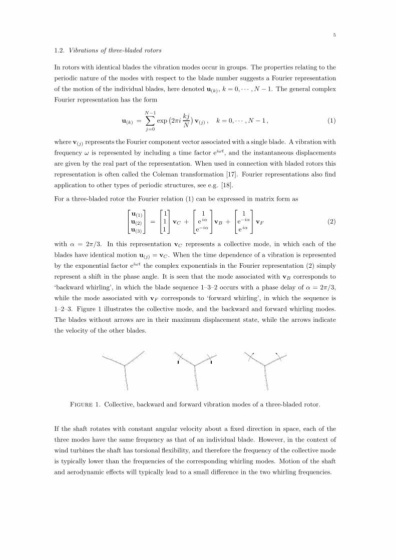
5
1.2. Vibrations of three-bladed rotors
In rotors with identical blades the vibration modes occur in groups. The properties relating to the
periodic nature of the modes with respect to the blade number suggests a Fourier representation
of the motion of the individual blades, here denoted u(𝑘), 𝑘 = 0, ⋅ ⋅ ⋅ , 𝑁 − 1. The general complex
Fourier representation has the form
u(𝑘) =
𝑁−1∑
𝑗=0
exp(
2𝜋𝑖𝑘𝑗
𝑁
)
v(𝑗) , 𝑘 = 0, ⋅ ⋅ ⋅ , 𝑁 − 1 , (1)
where v(𝑗) represents the Fourier component vector associated with a single blade. A vibration with
frequency 𝜔 is represented by including a time factor e𝑖𝜔𝑡, and the instantaneous displacements
are given by the real part of the representation. When used in connection with bladed rotors this
representation is often called the Coleman transformation [17]. Fourier representations also find
application to other types of periodic structures, see e.g. [18].
For a three-bladed rotor the Fourier relation (1) can be expressed in matrix form as
⎡
⎣
u(1)
u(2)
u(3)
⎤
⎦ =
⎡
⎣
111
⎤
⎦v𝐶 +
⎡
⎣
1e 𝑖𝛼
e−𝑖𝛼
⎤
⎦v𝐵 +
⎡
⎣
1e−𝑖𝛼
e 𝑖𝛼
⎤
⎦v𝐹 (2)
with 𝛼 = 2𝜋/3. In this representation v𝐶 represents a collective mode, in which each of the
blades have identical motion u(𝑗) = v𝐶 . When the time dependence of a vibration is represented
by the exponential factor e𝑖𝜔𝑡 the complex exponentials in the Fourier representation (2) simply
represent a shift in the phase angle. It is seen that the mode associated with v𝐵 corresponds to
‘backward whirling’, in which the blade sequence 1–3–2 occurs with a phase delay of 𝛼 = 2𝜋/3,
while the mode associated with v𝐹 corresponds to ‘forward whirling’, in which the sequence is
1–2–3. Figure 1 illustrates the collective mode, and the backward and forward whirling modes.
The blades without arrows are in their maximum displacement state, while the arrows indicate
the velocity of the other blades.
Figure 1. Collective, backward and forward vibration modes of a three-bladed rotor.
If the shaft rotates with constant angular velocity about a fixed direction in space, each of the
three modes have the same frequency as that of an individual blade. However, in the context of
wind turbines the shaft has torsional flexibility, and therefore the frequency of the collective mode
is typically lower than the frequencies of the corresponding whirling modes. Motion of the shaft
and aerodynamic effects will typically lead to a small difference in the two whirling frequencies.

6
1.3. Equations of motion
In the present paper the analysis is performed on a full rotor model in which the vector u contains
all degrees-of-freedom of the structural model. While detailed analysis propellers and helicopter
rotors may require use of a fully non-linear kinematic formulation, see e.g. [19], wind turbine
rotors in operational conditions can typically be analyzed with a partially non-linear theory, in
which accurate representation of the centrifugal forces is essential, [1]. In the rotating frame of
reference the discretized equations of motion can be written in the standard form, see e.g. [20],
Mu + 2Gu + Ku = f . (3)
The mass matrix is M, while 2G is the skew-symmetric gyroscopic matrix and K is the linearized
stiffness matrix. In the present problem the stiffness matrix consists of four contributions: the
elastic stiffness matrix K𝑒, the geometric stiffness matrix K𝑔 arising from the stiffening effects of
tension stresses, the negative stiffness C generated by the direct effect of the centrifugal force, and
in the case of variable angular velocity the angular acceleration stiffness G,
K = K𝑒 + K𝑔 − C + G. (4)
The total force vector
f = f𝑒 + f𝑐 − f𝑔 (5)
contains the external load f𝑒, the centrifugal forces f𝑐, and the gyroscopic forces −f𝑔. A detailed
derivation of the terms appearing in the equation of motion (3) in the form of a finite element
model with specialized beam elements is given in [21].
2. Vibrations of the Rotor
The control concept developed in this paper is based on resonant interaction between the rotor and
the controller, and it is therefore necessary first to establish some general properties of vibrations
of the rotor without the controller. This section gives a concise presentation of the theory and
properties of the dynamics of gyroscopic systems that are needed in the subsequent development
of the structural control.
2.1. Undamped gyroscopic vibrations
The additional damping to be introduced by the controller is needed because of small or negative
damping of the mode(s) in question. The calibration is therefore based on the corresponding
undamped vibrations. The undamped modes and the corresponding vibration frequencies are
found from the assumption of the existence of vibrations with the format
u(𝑡) = u𝑗 exp(𝜆𝑗𝑡) . (6)
where u𝑗 is typically a complex mode-shape vector, and the parameter 𝜆𝑗 determines the time
dependence. When this solution is substituted into the homogeneous form of the equation of

7
motion (3) the following quadratic eigenvalue problem is obtained
[M𝜆2𝑗 + 2G𝜆𝑗 + K ]u𝑗 = 0. (7)
In the case of non-gyroscopic motion G = 0, and the equation reduces to a linear eigenvalue
problem in 𝜆2𝑗 .
The gyroscopic eigenvalue problem is conveniently solved by forming an expanded eigenvalue
problem for the state-space variables, here collected in the state-space vector
z𝑇 = [ u𝑇 , u𝑇 ]. (8)
The equations of motion are typically expressed in the state-space format[
M 00 K
] [
uu
]
+
[
2G K−K 0
] [
uu
]
=
[
f0
]
, (9)
where a velocity identity has been introduced in a form involving the effective stiffness matrix K,
[22, 23, 20]. This format can be expressed in compact form as the set of linear first order equations
Az + Bz = F . (10)
with the 2𝑛× 2𝑛 matrices
A =
[
M 00 K
]
, B =
[
2G K−K 0
]
, (11)
and the expanded load vector
F𝑇 = [ f𝑇, 0 ]. (12)
The matrix A is symmetric, while B is skew-symmetric, when the system is undamped.
Free vibrations are now represented in the expanded format as
z(𝑡) = z𝑗 exp(𝜆𝑗𝑡) , (13)
where the eigenvalues and eigenvectors follow from the linear eigenvalue problem of the extended
equations of motion (10),[
B + 𝜆𝑗A]
z𝑗 = 0 . (14)
Alternative forms of the expanded linear eigenvalue problem exist, e.g. in terms of real vectors
[22, 23, 20] or in a hybrid state-space form in terms of the local displacements and global velocities,
where the last equation is a momentum balance expressed in terms of the mass matrix, [24].
However, in the present application the complex form of the mode shape vectors u𝑗 in connection
with the classic state-space format is convenient.
It is important for the present problem that the eigenvalues of an undamped gyroscopic system
are imaginary. This is most simply demonstrated by writing the state-space eigenvector z𝑗 of
the expanded eigenvalue problem (14) in terms of its real and imaginary parts, z𝑗 = x𝑗 + 𝑖y𝑗 .
Pre-multiplication of the expanded eigenvalue equation with z𝑇𝑗 gives the following expression for
the eigenvalue
𝜆𝑗 = −z𝑇𝑗 Bz𝑗
z𝑇𝑗 Az𝑗= −
2𝑖x𝑇𝑗 By𝑗
x𝑇𝑗 Ax𝑗 + y𝑇𝑗 Ay𝑗, (15)
where the last form follows from the symmetry of A and anti-symmetry of B. It follows im-
mediately from this formula that the eigenvalue 𝜆𝑗 is imaginary, and thus can be expressed in

8
terms of the real valued angular frequency 𝜔𝑗 as 𝜆𝑗 = 𝑖𝜔𝑗. It furthermore follows that if u𝑗 , 𝜆𝑗
constitute an eigen-pair, so does the complex conjugate pair u𝑗 , ��𝑗 = −𝑖𝜔𝑗. It follows from the
quadratic eigenvalue equation (7) that except for the very special case Gu𝑗 = 0, the eigenvector
u𝑗 is complex.
2.2. Frequency response analysis
A solution is now sought to the expanded non-homogeneous dynamic equation of motion (10) in
the form of an expansion in the 2𝑛 expanded mode shape vectors z𝑗 ,
z(𝑡) =2𝑛∑
𝑗=1
z𝑗 𝑞𝑗(𝑡). (16)
Let the time dependence be harmonic and of the form exp(𝜆𝑡) = exp(𝑖𝜔𝑡). Substitution of the
expansion (16) into the equation of motion (10) then gives
2𝑛∑
𝑗=1
(
B+ 𝜆A)
z𝑗 𝑞𝑗 = F. (17)
Pre-multiplication by z𝑇𝑘 gives
2𝑛∑
𝑗=1
z𝑇𝑘(
B+ 𝜆A)
z𝑗 𝑞𝑗 = z𝑇𝑘F = ��𝑘u𝑇𝑘 f , (18)
where the reduction of the load term follows from the state-space representation of the response
(8) and the load (12).
It follows from the linear eigenvalue problem (14) that the eigenvectors z𝑗 can be normalized to
satisfy the orthogonality relation
z𝑇𝑘Az𝑗 = 2𝛿𝑘𝑗 . (19)
An additional set of orthogonality then follows from the eigenvalue equations (14) in the form
z𝑇𝑘Bz𝑗 = −2𝜆𝑗 𝛿𝑘𝑗 . (20)
In these relations the factor 2 has been introduced to provide a smooth transition to the classic
non-gyroscopic solution for Ω → 0.
The orthogonality relations (19) and (20) reduce the response equation (18) to the following set
of equations for the individual component amplitudes 𝑞𝑘,
2(𝜆− 𝜆𝑘) 𝑞𝑘 = ��𝑘u𝑇𝑘 f . (21)
This relation determines the displacement amplitudes as
𝑞𝑘 =1
2
��𝑘𝜆− 𝜆𝑘
u𝑇𝑘 f =1
2
𝜔𝑘𝜔𝑘 − 𝜔
u𝑇𝑘 f . (22)
Substitution of these response amplitudes into the state-space expansion (16) gives
[
uu
]
= 12
2𝑛∑
𝑗=1
[
𝜆𝑗u𝑗u𝑗
]
𝜔𝑗𝜔𝑗 − 𝜔
u𝑇𝑗 f . (23)

9
The displacement response follows from the lower part of this state-space relation in the form
u = 12
2𝑛∑
𝑗=1
𝜔𝑗𝜔𝑗 − 𝜔
u𝑗u𝑇𝑗 f . (24)
In this representation each of the 2𝑛 eigenvector–eigenvalue pairs of the extended eigenvalue prob-
lem are represented by an individual term. However, when u𝑗 and 𝜆𝑗 = 𝑖𝜔𝑗 constitute an eigen-
pair, the combination of u𝑗 and ��𝑗 = −𝑖𝜔𝑗 also constitute a pair. Thus, the frequency response
can be represented by the 𝑛-term expansion
u = 12
𝑛∑
𝑗=1
( 𝜔𝑗𝜔𝑗 − 𝜔
u𝑗u𝑇𝑗 +
𝜔𝑗𝜔𝑗 + 𝜔
u𝑗u𝑇𝑗
)
f . (25)
Both of the matrices appearing within the parenthesis are Hermitean, but for gyroscopic sys-
tems the eigenvectors are complex, and the two matrices are not identical. When combining the
symmetric and skew-symmetric parts of the matrices, the following form of the solution is obtained
u =
𝑛∑
𝑗=1
[ 𝜔2𝑗
𝜔2𝑗 − 𝜔2
12
(
u𝑗u𝑇𝑗 + u𝑗u
𝑇𝑗
)
+𝜔 𝜔𝑗
𝜔2𝑗 − 𝜔2
12
(
u𝑗u𝑇𝑗 − u𝑗u
𝑇𝑗
)
]
f . (26)
The first term in the quare brackets is real and symmetric, and corresponds to the non-gyroscopic
case. The second term is skew-symmetric and imaginary, and is associated specifically with the
gyroscopic case via the complex eigenvectors.
2.3. Approximate frequency response formula
The calibration of the control system is based on the idea of a resonant mode, supplemented by
the quasi-static response from other modes with higher frequency. The idea of including the effect
of the additional flexibility provided by the high-frequency modes in the form of a quasi-static
approximation is classic within structural dynamics, see e.g. [25], and has been used successfully
in connection with active vibration control of stationary structures, e.g. in [15, 16]. In a rotating
frame with gyroscopic forces the mode shape vectors are complex, and the format of the frequency
response is modified as seen in (25) and (26), and this leads to a need for modifying the quasi-static
correction procedure.
The general frequency response formula (25) identifies a series expansion of the inverse of the
frequency dependent response equation matrix,
[K + 2𝑖𝜔G− 𝜔2M ]−1 = 12
𝑛∑
𝑗=1
( 𝜔𝑗𝜔𝑗 − 𝜔
u𝑗u𝑇𝑗 +
𝜔𝑗𝜔𝑗 + 𝜔
u𝑗u𝑇𝑗
)
. (27)
In particular, the limit 𝜔 = 0 represents the static flexibility in the form of the expansion
K−1 =𝑛∑
𝑗=1
12
(
u𝑗u𝑇𝑗 + u𝑗u
𝑇𝑗
)
. (28)
Now, let 𝜔𝑘 be the frequency of the resonant mode. When contributions from the lower-frequency
modes are neglected, and contributions from the higher-frequency modes are represented by their
quasi-static equivalent, the expansion (27) takes the form
[K + 2𝑖𝜔G− 𝜔2M ]−1 ≃ 12
( 𝜔𝑘𝜔𝑘 − 𝜔
u𝑘u𝑇𝑘 +
𝜔𝑘𝜔𝑘 + 𝜔
u𝑘u𝑇𝑘
)
+
𝑛∑
𝑗=𝑘+1
12
(
u𝑗u𝑇𝑗 + u𝑗u
𝑇𝑗
)
. (29)

10
The contribution from the resonant mode is now expressed in a form that emphasizes the Her-
mitean form of the original matrix around the resonance frequency 𝜔𝑘,
12
( 𝜔𝑘𝜔𝑘 − 𝜔
u𝑘u𝑇𝑘 +
𝜔𝑘𝜔𝑘 + 𝜔
u𝑘u𝑇𝑘
)
=𝜔2𝑘
𝜔2𝑘 − 𝜔2
u𝑘u𝑇𝑘 − 𝜔𝑘
𝜔𝑘 + 𝜔12
(
u𝑘u𝑇𝑘 − u𝑘u
𝑇𝑘
)
. (30)
In the present context the approximate response formulation is to be used in a frequency range
around 𝜔𝑘. In this range the first term in (30) dominates the second, which is therefore omitted
in the final approximation
[K + 2𝑖𝜔G− 𝜔2M ]−1 ≃ 𝜔2𝑘
𝜔2𝑘 − 𝜔2
u𝑘u𝑇𝑘 +
𝑛∑
𝑗=𝑘+1
12
(
u𝑗u𝑇𝑗 + u𝑗u
𝑇𝑗
)
. (31)
This approximation is mostly needed in connection with resonant response from one of the lower
modes, and it is therefore convenient to eliminate the summation over the higher modes by use of
(28), whereby
[K + 2𝑖𝜔G− 𝜔2M ]−1 ≃ 𝜔2𝑘
𝜔2𝑘 − 𝜔2
u𝑘u𝑇𝑘 +
[
K−1 −𝑘∑
𝑗=1
12
(
u𝑗u𝑇𝑗 + u𝑗u
𝑇𝑗
)
]
. (32)
It is seen that the modification due to the gyroscopic force term consists in using the Hermitean
product of the complex modes in the resonant term, and the symmetrized product in the quasi-
static correction.
2.4. Change of eigenfrequencies with rotation speed
In the present context it is of importance that the natural vibration frequencies change with the
angular velocity of the rotorΩ. A simple estimate of the relative change of natural frequency can be
obtained from a perturbation analysis of the quadratic eigenvalue problem (7). The non-rotating
state ∣Ω∣ = 0 is used as reference state for a mode shape u0 with angular vibration frequency 𝝎0.
A direct first order perturbation leads to the following form for the angular vibration frequency 𝜔
at the angular rotation frequency Ω
𝜔2
𝜔20
=u𝑇0 K(Ω)u0
u𝑇0 K0u0= 1 +
u𝑇0 (K𝑔 − C )∣Ω∣=1u0
u𝑇0 K0u0Ω2 , (33)
where K(Ω) is the effective stiffness matrix at the rotation frequency Ω = ∣Ω∣, while K0 is at
standstill with Ω = 0. Thus, the formula (33) makes use of the ratio between the modal stiffness
at the rotation frequency Ω and the modal stiffness at Ω = 0. The change of stiffness comes from
the geometric stiffness matrix K𝑔 and the centrifugal force matrix C. Both of these components
are quadratic in Ω, leading to the last expression. The change in natural frequency of a rotor due
to the rotational stiffening effect is illustrated in [26]. In the present context for a wind turbine
rotor the increase in geometric stiffness will typically outweigh the stiffness reduction from the
centrifugal force matrix, leading to an increase of vibration frequency with increasing rotation
speed. This is discussed and illustrated in the example in Section 5.

11
3. Control System
The vibration control is implemented via actuators which impose the control force vector f𝜂 on
the structure. After introduction of the control force the equation of motion (3) takes the form
(
K+ 2𝑖𝜔G− 𝜔2M)
u+ f𝜂 = f . (34)
In the present context the control forces are intended to reduce the vibration intensity of a group
of vibration modes such as the combined vibration in the first in-plane collective and associated
forward and backward whirling modes discussed in Section 1 and illustrated in Fig. 1.
The natural frequency of the collective mode is typically smaller than the natural frequency of the
two whirling modes due to the rotational flexibility of the drivetrain. Thus, resonant control, based
on the natural frequencies of the modes, must address the whirling mode and the set of the two
whirling modes separately. The control is implemented via identical collocated sensor/actuator
pairs on each of the three blades. In its simplest form the sensor/actuator connects two degrees
of freedom of a blade, typically by a vector of the form
w𝑘 = [ 0, ⋅ ⋅ ⋅ , 1, 0, ⋅ ⋅ ⋅ ,−1, 0, ⋅ ⋅ ⋅ ]𝑇 , 𝑘 = 1, 2, 3, (35)
where the subscript 𝑘 = 1, 2, 3 denotes the blade number, and the ±1 coefficients form the differ-
ence between the two degrees of freedom of this blade.
3.1. Feedback from collective mode
The connectivity array of the collective mode is defined by the mean value of the corresponding
arrays for the individual blades,
w𝑐 =13
(
w1 +w2 +w3
)
. (36)
This connectivity array defines an average over the three blades of the displacement difference
registered by the sensor(s) on the individual blades. The averaged displacement w𝑇𝑐u defines a
control variable 𝜂𝑐 for the collective mode by the frequency relation
𝐺 𝑐𝜂𝑢(𝜔)w
𝑇𝑐u+𝐺 𝑐
𝜂𝜂(𝜔)𝜂𝑐 = 0. (37)
In this equation 𝐺 𝑐𝜂𝜂(𝜔) is a resonant second-order filter,
𝐺 𝑐𝜂𝜂(𝜔) = 𝜔2
𝑐 − 𝜔2 + 2𝑖𝜁𝑐𝜔𝑐𝜔. (38)
Here 𝜔𝑐 is the controller frequency of the collective mode, which must be tuned to the natural
frequency 𝜔𝑐,𝑛 of the free collective vibration mode as in Section 4.1, where also the damping
parameter 𝜁𝑐 is calibrated. 𝐺𝑐𝜂𝑢(𝜔) is a second-order filter, representing the coupling between the
control variable and the structure. It may be chosen to implement acceleration feedback by
𝐺 𝑐𝜂𝑢(𝜔) = 𝜔2. (39)
Alternatively, displacement feedback may be implemented by selecting 𝐺 𝑐𝜂𝑢(𝜔) = 𝜔2
𝑐 , as discussed
in [15]. Only acceleration feedback will be considered explicitly here.

12
A special case occurs if the displacement field is given completely by the collective mode shape u𝑐
in the form u = u𝑐𝑞𝑐, where 𝑞𝑐 is the corresponding modal coordinate. In this case the frequency
relation (37) takes the form
𝐺 𝑐𝜂𝑢(𝜔)𝜈𝑐𝑞𝑐 +𝐺 𝑐
𝜂𝜂(𝜔)𝜂𝑐 = 0, (40)
where
𝜈𝑐 = w𝑇𝑐 u𝑐 (41)
is the modal connectivity parameter of the collective mode, giving the displacement of the mode-
shape vector over the controller. For flexible structures the control parameters should be calibrated
from the full displacement vector u which contains additional contributions from other modes that
are excited by the actuator forces. This is discussed in detail in Section 4, but first the feedback
format of the whirling modes must be presented.
3.2. Feedback from whirling modes
The whirling modes involve different displacements in each of the blades, and therefore require a
connectivity array with contributions from each of the blades. When the mean contribution from
the collective mode is subtracted, the whirling mode connectivity array takes the form
W = 13 [w1 −w𝑐,w2 −w𝑐,w3 −w𝑐 ], (42)
where each of the three columns correspond to one of the blades. There are three components in
the representation of the whirling modes, and although the introduction of w𝑐 leads to a linear
relation between these components, the analysis is simplified by retaining three components in the
analysis. In the case of the whirling modes the three displacement components are extracted in the
form W𝑇u. These displacement components are related to the control variables 𝜼 = [ 𝜂1, 𝜂2, 𝜂3]𝑇
by the frequency relation
𝐺𝑤𝜂𝑢(𝜔)W
𝑇u+𝐺𝑤𝜂𝜂(𝜔)𝜼 = 0. (43)
In this relation 𝐺𝜂𝜂(𝜔) is a common scalar resonant second-order filter for the whirling modes,
𝐺𝑤𝜂𝜂(𝜔) = 𝜔2
𝑤 − 𝜔2 + 2𝑖𝜁𝑤𝜔𝑤𝜔. (44)
Here 𝜔𝑤 is the controller frequency of the whirling modes, which must be tuned to the natural
frequency 𝜔𝑤,𝑛 of the free whirling vibration modes, and 𝜁𝑤 is the damping parameter for the
whirling modes. The whirling modes will have acceleration feedback, represented by
𝐺𝑤𝜂𝑢(𝜔) = 𝜔2. (45)
Also this can be changed to displacement feedback.
At whirling mode resonance the displacement field will be dominated by a combination of the
whirling modes, combined in u = u𝑤𝑞𝑤, where 𝑞𝑤 is the modal coordinate. When this represen-
tation is substituted, the frequency relation (43) takes the form
𝐺𝑤𝜂𝑢(𝜔)W
𝑇u𝑤𝑞𝑤 +𝐺𝑤𝜂𝜂(𝜔)𝜼 = 0. (46)
13
This relation determines the relative magnitude of the control variable components by 𝜼 ∝ W𝑇u𝑤.
Thus, a modal connectivity factor can be introduced for the three components of the whirling
motion,
𝝂𝑤 = W𝑇u𝑤. (47)
The relation between the components of the control variables 𝜼 can then be expressed in normalized
form as
𝜼 = 𝜈−1𝑤 𝝂𝑤 𝜂𝑤, 𝜈𝑤 = (𝝂𝑇𝑤𝝂𝑤)
1/2. (48)
It is noted that if 𝝂𝑤 corresponds to one of the whirling modes, e.g. forward whirling, the complex
conjugate 𝝂𝑤 corresponds to the other, backward whirling. Thus, the two whirling modes are
equally represented in the parameter 𝜈𝑤.
Pre-multiplication of the three-component whirling mode feedback equation (46) by 𝝂𝑇𝑤 then re-
duces to the single scalar equation
𝐺𝑤𝜂𝑢(𝜔)𝜈𝑤𝑞𝑤 +𝐺𝑤
𝜂𝜂(𝜔)𝜂𝑤 = 0 . (49)
This equation is of the same form as the feedback equation (40) for the collective mode, and
thus the calibration of the two sets of control parameters follow essentially the same procedure as
described in Section 4.
3.3. Control force equation
The control force has components from both the collective and the whirling modes. These are
filtered by the frequency functions 𝐺 𝑐𝑢𝜂(𝜔) and 𝐺 𝑐
𝑢𝜂(𝜔), respectively. The system is designed as
collocated, whereby the force components are generated by the same index arrays used to extract
the control signal, and the controller force therefore has the form
f𝜂 = 𝐺 𝑐𝑢𝜂(𝜔)w𝑐𝜂𝑐 + 𝐺𝑤
𝑢𝜂(𝜔)W𝜼. (50)
This representation is introduced into the equation of motion (34), and the total set of equations
then consist of the structural equation of motion plus the equations (37) and (46) for the controller
signals. The corresponding reduced control equations (40) and (49) are used for calibrating the
controller functions 𝐺𝜂𝜂(𝜔), 𝐺𝜂𝑢(𝜔) and 𝐺𝑢𝜂(𝜔) for the collective and the whirling modes as
discussed in the next section.
4. Controller Calibration
The two components of the resulting control force (50), addressing the collective and the whirling
modes, respectively, are calibrated individually in the following. The optimal control parameters
for the basic calibration without the quasi-static correction for background flexibility are presented
first, and then these results are modified to take the effect of background flexibility into account.
The calibration is a generalization to complex modes of the procedure described in detail in [15, 16],
which has been used for damping of a single wind turbine blade in [21].

14
4.1. Basic calibration of collective mode
The governing equations for the resonant control of the collective mode are obtained by combining
the equation of motion (34), the control force described by the first term in (50), and the scalar filter
equation in (40). In this initial calibration procedure the response is assumed to be fully described
by the collective mode, u = u𝑐𝑞𝑐, and the dynamic part of (32). Hereby, the homogeneous scalar
equations governing the control of the collective mode can be written as
(𝜔2𝑐,𝑛 − 𝜔2) 𝜈𝑐 𝑞𝑐 + 𝜔2
𝑐,𝑛 ∣𝜈𝑐∣2𝐺𝑐𝑢𝜂(𝜔) 𝜂𝑐 = 0,
𝐺𝑐𝜂𝑢(𝜔) 𝜈𝑐 𝑞𝑐 + 𝐺𝑐
𝜂𝜂(𝜔) 𝜂𝑐 = 0,(51)
where ∣𝜈𝑐∣ = (𝜈𝑐𝜈𝑐)1/2 is the magnitude of the modal connectivity parameter 𝜈𝑐. For acceleration
feedback with 𝐺𝑐𝜂𝑢(𝜔) = 𝜔2 the corresponding control function 𝐺𝑐
𝑢𝜂(𝜔) contains a constant and a
linear term with gain parameters 𝛼𝑐 and 𝛽𝑐, respectively,
𝜔2𝑐,𝑛 ∣𝜈𝑐∣2𝐺𝑐
𝑢𝜂(𝜔) = 𝛼𝑐 𝜔2𝑐 + 𝛽𝑐 2𝑖𝜁𝑐𝜔𝑐𝜔 . (52)
The normalization of 𝐺𝑐𝑢𝜂(𝜔) by 𝜔2
𝑐,𝑛 ∣𝜈𝑐∣2 is suggested by the second term of the first equation in
(51), and the control variable then only appears in the combination 𝜂𝑐/𝜈𝑐. This leaves a formu-
lation, in which 𝛼𝑐 can be considered as a gain parameter of the controller, while the parameters
𝜔𝑐, 𝛽𝑐 and 𝜁𝑐 should be determined to yield optimal control properties.
The coupled equations (51) are a generalized form of the frequency response equations of a tuned
mass damper, analyzed in detail in [27]. The gain parameter 𝛼𝑐 plays the role of the mass ratio in
the tuned mass damper. The resonant control force splits the original single mode into two modes,
and the optimal solution corresponds to equal damping of these two modes. This provides two
equations, essentially determining the coupling coefficient 𝛽𝑐 and the resonant controller frequency
𝜔𝑐. The controller damping parameter 𝜁𝑐 is then determined from the frequency response prop-
erties. This procedure results in the following optimal parameters in terms of the gain parameter
𝛼𝑐:
𝛽𝑐 = 𝛼𝑐 , 𝜔𝑐 =𝜔𝑐,𝑛1 + 𝛼𝑐
, 𝜁2𝑐 =𝛼𝑐
2(1 + 𝛼𝑐). (53)
These expressions, corresponding to calibration without background flexibility, are summarized in
the first row of Table 1.
Resonant control is typically advantageous when additional damping Δ𝜁 is needed for lightly
damped modes of the structures, such as e.g. the edgewise vibration modes of a wind turbine
rotor. The present calibration procedure secures equal modal damping of the targeted mode,
which in this case is the collective mode. For optimal calibration the two modes associated with
the collective vibration form receives half of the damping ratio associated with the controller, [27],
Δ𝜁𝑐,𝑛 ≃ 12 𝜁𝑐 . (54)
This means that the desired damping is obtained by choosing 𝜁𝑐 as twice the desired additional
damping for the targeted mode. The expression for 𝜁𝑐 in (53) can then be solved for the gain
parameters 𝛼, which finally determines the remaining control parameters 𝛼𝑐, 𝛽𝑐 and 𝜔𝑐. This

15
Table 1. Calibration with gain parameter 𝛼.
𝛼𝑐,𝑤 𝛽𝑐,𝑤
(
𝜔
𝜔𝑛
)2
𝑐,𝑤
(
𝜁𝜔
𝜔𝑛
)
𝑐,𝑤
Basic 𝛼 𝛼1
(1 + 𝛼)2
√
𝛼
2(1 + 𝛼)3
Full 𝛼𝛼
1 + 𝜅𝛼
1
1− 𝜅𝛼
(1 + 𝛼)2
1
(1 + 𝛼)21 + 𝜅𝛼
1− 𝜅𝛼
(1 + 𝛼)2
√
𝛼
2(1 + 𝛼)3
design sequence can also be applied for the control of the whirling modes, as demonstrated for the
control of the wind turbine rotor in Section 5.
4.2. Basic calibration of whirling modes
For the whirling modes the control equations are obtained by combining the equation of motion
(34), the control force described by the second term in (50), and the filter equation in (49). The
response is in this case assumed to be represented by the whirling mode, u = u𝑤𝑞𝑤, and again
only the dynamic part of (32) is included. Hereby, the scalar equations for the control of the
whirling modes can be written in normalized form as
(𝜔2𝑤,𝑛 − 𝜔2) 𝜈𝑤 𝑞𝑤 + 𝜔2
𝑤,𝑛 𝜈2𝑤𝐺
𝑤𝑢𝜂(𝜔) 𝜂𝑤 = 0,
𝐺𝑤𝜂𝑢(𝜔) 𝜈𝑤 𝑞𝑤 + 𝐺𝑤
𝜂𝜂(𝜔) 𝜂𝑤 = 0,(55)
where the normalized scalar parameters 𝜈𝑤 and 𝜂𝑤 are defined in (48). The format of the frequency
function 𝐺𝑤𝑢𝜂(𝜔) is identical to that in (52) for the collective mode,
𝜔2𝑤,𝑛 𝜈
2𝑤 𝐺𝑤
𝑢𝜂(𝜔) = 𝛼𝑤 𝜔2𝑤 + 𝛽𝑤 2𝑖𝜁𝑤𝜔𝑤𝜔. (56)
With this normalization the equations only depend on the control variable in the combination
𝜂𝑤/𝜈𝑤. The governing equations for the whirling modes in (55)–(56) are equivalent to those in
(51)–(52) for the collective mode. When 𝛼𝑤 is taken as gain parameter in this case, the remaining
parameters 𝛽𝑤, 𝜔𝑤 and 𝜁𝑤 are given by the expressions in (53), when replacing the subscript 𝑐 by
𝑤. Thus the first row in Table 1 applies to both the controllers of the collective and the whirling
modes.
4.3. Accounting for background flexibility
In modal control of flexible structures the the sensors and actuators typically interact with defor-
mations from non-targeted modes thereby contaminating the simple single mode control scheme.
When using a small number of sensors/actuaors this effect can be an important aspect in the
design of the control scheme, see e.g. [28]. In the analysis leading to the scalar equations (51)
and (55) for the collective and whirling modes, respectively, the response is assumed to be fully
represented by the targeted mode alone. However, in general the structural response contains
contributions from all vibration modes of the system. The displacement generated by the control
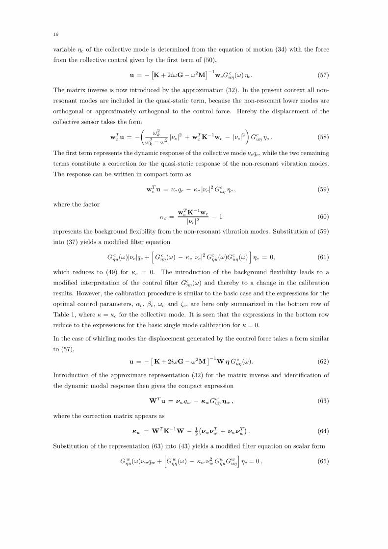
16
variable 𝜂𝑐 of the collective mode is determined from the equation of motion (34) with the force
from the collective control given by the first term of (50),
u = −[
K+ 2𝑖𝜔G− 𝜔2M]
−1w𝑐𝐺
𝑐𝑢𝜂(𝜔) 𝜂𝑐. (57)
The matrix inverse is now introduced by the approximation (32). In the present context all non-
resonant modes are included in the quasi-static term, because the non-resonant lower modes are
orthogonal or approximately orthogonal to the control force. Hereby the displacement of the
collective sensor takes the form
w𝑇𝑐 u = −
(
𝜔2𝑘
𝜔2𝑘 − 𝜔2
∣𝜈𝑐∣2 + w𝑇𝑐 K
−1w𝑐 − ∣𝜈𝑐∣2)
𝐺𝑐𝑢𝜂 𝜂𝑐 . (58)
The first term represents the dynamic response of the collective mode 𝜈𝑐𝑞𝑐, while the two remaining
terms constitute a correction for the quasi-static response of the non-resonant vibration modes.
The response can be written in compact form as
w𝑇𝑐 u = 𝜈𝑐 𝑞𝑐 − 𝜅𝑐 ∣𝜈𝑐∣2 𝐺𝑐
𝑢𝜂 𝜂𝑐 , (59)
where the factor
𝜅𝑐 =w𝑇𝑐 K
−1w𝑐
∣𝜈𝑐∣2− 1 (60)
represents the background flexibility from the non-resonant vibration modes. Substitution of (59)
into (37) yields a modified filter equation
𝐺 𝑐𝜂𝑢(𝜔)∣𝜈𝑐∣𝑞𝑐 +
[
𝐺 𝑐𝜂𝜂(𝜔) − 𝜅𝑐 ∣𝜈𝑐∣2 𝐺𝑐
𝜂𝑢(𝜔)𝐺𝑐𝑢𝜂(𝜔)
]
𝜂𝑐 = 0, (61)
which reduces to (49) for 𝜅𝑐 = 0. The introduction of the background flexibility leads to a
modified interpretation of the control filter 𝐺𝑐𝜂𝜂(𝜔) and thereby to a change in the calibration
results. However, the calibration procedure is similar to the basic case and the expressions for the
optimal control parameters, 𝛼𝑐, 𝛽𝑐, 𝜔𝑐 and 𝜁𝑐, are here only summarized in the bottom row of
Table 1, where 𝜅 = 𝜅𝑐 for the collective mode. It is seen that the expressions in the bottom row
reduce to the expressions for the basic single mode calibration for 𝜅 = 0.
In the case of whirling modes the displacement generated by the control force takes a form similar
to (57),
u = −[
K+ 2𝑖𝜔G− 𝜔2M]
−1W𝜼𝐺 𝑐
𝑢𝜂(𝜔). (62)
Introduction of the approximate representation (32) for the matrix inverse and identification of
the dynamic modal response then gives the compact expression
W𝑇u = 𝝂𝑤𝑞𝑤 − 𝜿𝑤𝐺𝑤𝑢𝜂 𝜼𝑤 , (63)
where the correction matrix appears as
𝜿𝑤 = W𝑇K−1W − 12
(
𝝂𝑤𝝂𝑇𝑤 + 𝝂𝑤𝝂
𝑇𝑤
)
. (64)
Substitution of the representation (63) into (43) yields a modified filter equation on scalar form
𝐺𝑤𝜂𝑢(𝜔)𝜈𝑤𝑞𝑤 +
[
𝐺𝑤𝜂𝜂(𝜔) − 𝜅𝑤 𝜈2𝑤𝐺𝑤
𝜂𝑢𝐺𝑤𝑢𝜂
]
𝜂𝑐 = 0 , (65)

17
where the scalar correction factor is given as
𝜅𝑤 =𝝂𝑇𝑤𝜿𝑤𝝂𝑤
𝜈4𝑤=
𝝂𝑇𝑤W𝑇K−1W𝝂𝑤
𝜈4𝑤− 1 . (66)
It is noted that for undamped gyroscopic systems this scalar factor is real-valued. The modified
filter equation (65) is equivalent to that in (61) for the collective mode, and the optimal control
parameters for the whirling mode are given by the expressions in the bottom row of Table 1 with
𝜅 = 𝜅𝑤.
4.4. Implementation
The equations of motion for the combined structure-control system are obtained by substitution
of the control force expression (50) into the equation of motion (34). This equation must be
supplemented by the equation (37) for the control of the collective mode and (43) for the whirling
modes. The frequency functions defining the control are defined in (38), (39) and (52) for the
collective mode, and in (44), (45) and (56) for the whirling modes.
The coupled equations of motion can be written in matrix form as
M∗u∗ + D∗u∗ + K∗u∗ = f∗ , (67)
where the asterisk ∗ refers to an expanded format, where the augmented vector u∗ contains both
the structural and the control variables,
u𝑇∗= [u𝑇 , 𝜼𝑇 , 𝜂𝑐 ] . (68)
The vector 𝜼 contains the three control variables addressing the whirling modes, while 𝜂𝑐 is the
scalar control variable for the collective mode. In the expanded format the system matrices are
given as
M∗ =
⎡
⎢
⎣
M 0 0
−W𝑇 I 0
−w𝑇𝑐 0 1
⎤
⎥
⎦, D∗ =
⎡
⎢
⎣
2G 𝑔𝑤𝛽W 𝑔𝑐𝛽w𝑐
0 𝑔𝑤𝜁 I 0
0 0 𝑔𝑐𝜁
⎤
⎥
⎦, K∗ =
⎡
⎢
⎣
K 𝑔𝑤𝛼W 𝑔𝑐𝛼w𝑐
0 𝑔𝑤𝜔 I 0
0 0 𝑔𝑐𝜔
⎤
⎥
⎦. (69)
The effective system parameters are defined as
𝑔𝛼 =𝛼𝜂
(𝜔𝑛𝜈)2𝜔2𝜂 , 𝑔𝛽 =
𝛽𝜂(𝜔𝑛𝜈)2
2𝜁𝜂𝜔𝜂 , 𝑔𝜁 = 2𝜁𝜂𝜔𝜂 , 𝑔𝜔 = 𝜔2𝜂 , (70)
where superscripts 𝑐 and 𝑤 are implied, while 𝜔𝑛𝜈 = 𝜔𝑐,𝑛∣𝜈𝑐∣ for the control of the collective modeand 𝜔𝑛𝜈 = 𝜔𝑐,𝑤𝜈𝑤 for the whirling modes. The augmented force vector is f𝑇
∗= [ f𝑇 , 0𝑇 , 0 ]. It is
noted that the present formulation does not include any delays in the controller system. However,
in principle these effects can be included in the present format via additional differential relations,
if needed.
5. Active Control of Wind Turbine Rotor
In this section the theory is illustrated by application to a three-bladed wind turbine rotor with
a diameter of 86m shown in Fig. 2 with an active strut mounted near the root of each blade.
First the structural properties and dynamics of the rotor without control are presented. Then a
controller system with a single active strut at the root of each blade is described and calibrated
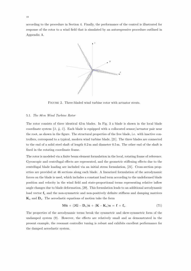
18
according to the procedure in Section 4. Finally, the performance of the control is illustrated for
response of the rotor to a wind field that is simulated by an autoregressive procedure outlined in
Appendix A.
x
y
z
Figure 2. Three-bladed wind turbine rotor with actuator struts.
5.1. The 86m Wind Turbine Rotor
The rotor consists of three identical 42m blades. In Fig. 3 a blade is shown in the local blade
coordinate system {��, 𝑦, 𝑧}. Each blade is equipped with a collocated sensor/actuator pair near
the root, as shown in the figure. The structural properties of the free blade, i.e. with inactive con-
trollers, correspond to a typical, modern wind turbine blade, [21]. The three blades are connected
to the end of a solid steel shaft of length 0.2m and diameter 0.5m. The other end of the shaft is
fixed in the rotating coordinate frame.
The rotor is modeled via a finite beam element formulation in the local, rotating frame of reference.
Gyroscopic and centrifugal effects are represented, and the geometric stiffening effects due to the
centrifugal blade loading are included via an initial stress formulation, [21]. Cross-section prop-
erties are provided at 46 sections along each blade. A linearized formulation of the aerodynamic
forces on the blade is used, which includes a constant load term according to the undeformed blade
position and velocity in the wind field and state-proportional terms representing relative inflow
angle changes due to blade deformation, [29]. This formulation leads to an additional aerodynamic
load vector f𝑎 and the non-symmetric and non-positively definite stiffness and damping matrices
K𝑎 and D𝑎. The aeroelastic equations of motion take the form
Mu + (2G−D𝑎)u + (K−K𝑎)u = f + f𝑎. (71)
The properties of the aerodynamic terms break the symmetric and skew-symmetric form of the
undamped system (9). However, the effects are relatively small and as demonstrated in the
present example, the resonant controller tuning is robust and exhibits excellent performance for
the damped aeroelastic system.

19
��
𝑦
𝑧
𝑄𝜂
−𝑄𝜂
Figure 3. Rotor blade in the local coordinate system with an active strut at-tached at two cross-sections near the root.
The blades are modeled using 𝑁𝑒𝑙 = 8 elements per blade of the type described in detail in [21], and
the shaft is represented by a single element. The modal properties of the system (71) are obtained
as a linear perturbation from a stationary state including structural forces with geometric stiffness,
and centrifugal and aerodynamic forces. The modes and frequencies are obtained by solving
the state-space eigenvalue problem (14), including the state-dependent aerodynamic terms. The
eigenfrequencies 𝜔𝑗 and the aeroelastic damping ratios 𝜁𝑗 are shown in Table 2. Modes 1-3 are the
first flap-wise collective and whirling modes, that are dominated by displacements perpendicular
to the rotor plane with local components 𝑞𝑦. The flap-wise modes are seen to be fairly strongly
damped due to their significant impact on the flow pattern. Modes 4–6 constitute the first group
of edge-wise vibration modes, with a collective mode 4, backward whirling in mode 5, and forward
whirling in mode 6. These modes are seen to be weakly damped by aerodynamics, as they are
dominated by displacements along the chord of the blade cross-sections. Modes 7–9 are the second
flap-wise blade bending modes and modes 10–12 are the second edge-wise bending modes.
Table 2. Rotor eigenfrequencies and linear aerodynamic damping ratios.
𝑗 1 2 3 4 5 6 7 8 9 10 11 12
𝜔𝑗 6.155 6.174 6.234 8.543 9.142 9.154 16.31 16.31 16.57 25.64 27.59 27.59
𝜁𝑗 0.425 0.421 0.416 0.014 0.006 0.006 0.164 0.164 0.162 0.001 0.001 0.001
The rotor eigenfrequencies vary with the angular rotor velocity Ω, and for the present rotor
the development is shown in Fig. 4 for modes 1, 4, 7 and 10. The values are obtained from
0 0.5 1 1.5 2
1
1.02
1.04
1.06
1.08
1.1 ω1/ω0
1
ω4/ω0
4
ω7/ω0
7
ω10/ω0
10
Ω𝑦 [ rad ]
𝜔𝑗/𝜔
0 𝑗
Figure 4. Eigenfrequencies as function of rotor angular velocity Ω𝑦. Markersfrom the eigenvalue problem (14), curves from the analytical expression (33).
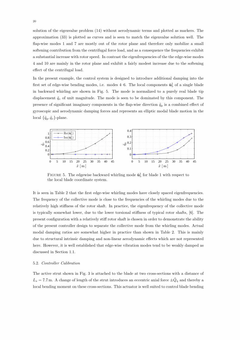
20
solution of the eigenvalue problem (14) without aerodynamic terms and plotted as markers. The
approximation (33) is plotted as curves and is seen to match the eigenvalue solution well. The
flap-wise modes 1 and 7 are mostly out of the rotor plane and therefore only mobilize a small
softening contribution from the centrifugal force load, and as a consequence the frequencies exhibit
a substantial increase with rotor speed. In contrast the eigenfrequencies of the the edge-wise modes
4 and 10 are mainly in the rotor plane and exhibit a fairly modest increase due to the softening
effect of the centrifugal load.
In the present example, the control system is designed to introduce additional damping into the
first set of edge-wise bending modes, i.e. modes 4–6. The local components u15 of a single blade
in backward whirling are shown in Fig. 5. The mode is normalized to a purely real blade tip
displacement 𝑞𝑧 of unit magnitude. The mode is seen to be dominated by this component. The
presence of significant imaginary components in the flap-wise direction 𝑞𝑦 is a combined effect of
gyroscopic and aerodynamic damping forces and represents an elliptic modal blade motion in the
local {𝑞𝑦, 𝑞𝑧}-plane.
0 5 10 15 20 25 30 35 40 45
00.20.40.60.8
1 Re(u1
5)
Im(u1
5)
0 5 10 15 20 25 30 35 40 45
0
0.1
0.2
0.3
0.4
�� [ m ]�� [ m ]
𝑞 𝑧 𝑞 𝑦
Figure 5. The edgewise backward whirling mode u15 for blade 1 with respect to
the local blade coordinate system.
It is seen in Table 2 that the first edge-wise whirling modes have closely spaced eigenfrequencies.
The frequency of the collective mode is close to the frequencies of the whirling modes due to the
relatively high stiffness of the rotor shaft. In practice, the eigenfrequency of the collective mode
is typically somewhat lower, due to the lower torsional stiffness of typical rotor shafts, [6]. The
present configuration with a relatively stiff rotor shaft is chosen in order to demonstrate the ability
of the present controller design to separate the collective mode from the whirling modes. Actual
modal damping ratios are somewhat higher in practice than shown in Table 2. This is mainly
due to structural intrinsic damping and non-linear aerodynamic effects which are not represented
here. However, it is well established that edge-wise vibration modes tend to be weakly damped as
discussed in Section 1.1.
5.2. Controller Calibration
The active strut shown in Fig. 3 is attached to the blade at two cross-sections with a distance of
𝐿𝑠 = 7.7m. A change of length of the strut introduces an eccentric axial force ±��𝜂 and thereby a
local bending moment on these cross-sections. This actuator is well suited to control blade bending

21
modes, including in particular the first group of edge-wise vibration modes. For this purpose the
eccentricity of the strut is chosen to impose bending moments about the local 𝑦-axis. The optimal
polar angle between the 𝑧-axis and the direction to the strut is nearly the same for the three
edge-wise modes, and the value 𝜃𝑠/𝜋 = 0.46 is chosen in all three blades to conserve symmetry.
The control system is calibrated by the procedure described in Section 4, including the effect of
the background flexibility. The controller is designed to introduce the desired additional damp-
ing ratio to the collective mode Δ𝜁𝑐 = 0.06 and the additional damping ratio Δ𝜁𝑤 = 0.06 to
the whirling modes. The resulting parameters are given in Table 3. The basic controller tun-
ing involves a reduction of the controller frequencies 𝜔𝑐,𝑤 relative to the modal eigenfrequency,
while the quasi-static correction prescribes a relative increase. In the present case the resulting
controller frequencies are slightly higher than the corresponding undamped structural frequencies,
with 𝜔𝑐/𝜔4 = 9.075/8.543 = 1.062 and 𝜔𝑤/𝜔5 = 9.564/9.142 = 1.046. Also, the resulting con-
troller damping ratios are seen to be slightly higher than the basic value of 𝜁𝑐,𝑤 ≃ 2Δ𝜁4,5 = 0.12.
Table 3. Control parameters for Δ𝜁4,5 = 0.06.
𝛼𝑐,𝑤 𝛽𝑐,𝑤 𝜔𝑐,𝑤 𝜁𝑐,𝑤 𝜈 𝜅
Collective 0.0297 0.0253 9.075 0.1541 1.374e-5 5.867
Whirling 0.0297 0.0259 9.564 0.1482 2.558e-5 4.941
The structural frequency response of the collective and the two whirling modes are shown in the
upper part of Fig. 6. The dynamic amplification of a blade tip response is evaluated for a harmonic
load proportional to the individual mode shape, f = u𝑗𝑒𝑖𝜔𝑡. The free response, shown with a thin
full line displays significant resonant amplification, while the damped response, shown with a
thick full line displays equally damped modes with low dynamic amplification and the desired
flat plateau at resonance. The dashed curves show the response obtained when the correction for
quasi-static background flexibility is not included, i.e. with 𝜅𝑐,𝑤 = 0. Clearly, this correction is
decisive for optimal calibration of the present control system. The importance of the quasi-static
correction is represented by the magnitude of the parameter 𝜅, and examples in [16] for a building
structure show the parameter range 𝜅 ≃ 1–10, depending on how directly the sensor/actuator pair
is addressing the targeted mode.
The lower part of Fig. 6 shows the frequency responses of the imposed controller moments ��𝜂 =
��𝜂𝑑𝑧 , where 𝑑𝑧 is the local 𝑧-wise position coordinate of the sensor/actuator pair. The values are
normalized with respect to the static blade root moments about the local 𝑦-axis ��0𝑦 . The slightly
inclined plateau is similar to the ideal optimal results presented in [15].
The response is calculated by use of the combined structure–controller equations (67). The eigen-
value problem associated with equation (67) is solved for the four possible combinations of active
or in-active controllers and the associated modal properties of the closed-loop system are listed
in Table 4. The modal properties for zero gain, 𝛼𝑐 = 𝛼𝑤 = 0 corresponds to Δ𝜁𝑐,𝑤 = 0 and
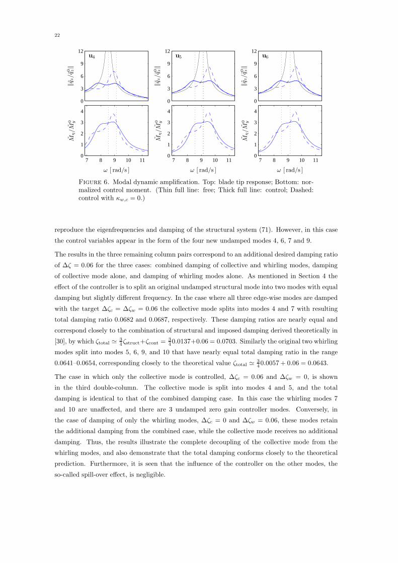
22
0
3
6
9
12u4
0
3
6
9
12u5
0
3
6
9
12u6
7 8 9 10 110
1
2
3
4
7 8 9 10 110
1
2
3
4
7 8 9 10 110
1
2
3
4
𝜔 [ rad/s ]𝜔 [ rad/s ]𝜔 [ rad/s ]
∥𝑞 𝑧/𝑞0 𝑧∥
∥𝑞 𝑧/𝑞0 𝑧∥
∥𝑞 𝑧/𝑞0 𝑧∥
𝑀𝜂/𝑀
0 𝑦
𝑀𝜂/𝑀
0 𝑦
𝑀𝜂/𝑀
0 𝑦
Figure 6. Modal dynamic amplification. Top: blade tip response; Bottom: nor-malized control moment. (Thin full line: free; Thick full line: control; Dashed:control with 𝜅𝑤,𝑐 = 0.)
reproduce the eigenfrequencies and damping of the structural system (71). However, in this case
the control variables appear in the form of the four new undamped modes 4, 6, 7 and 9.
The results in the three remaining column pairs correspond to an additional desired damping ratio
of Δ𝜁 = 0.06 for the three cases: combined damping of collective and whirling modes, damping
of collective mode alone, and damping of whirling modes alone. As mentioned in Section 4 the
effect of the controller is to split an original undamped structural mode into two modes with equal
damping but slightly different frequency. In the case where all three edge-wise modes are damped
with the target Δ𝜁𝑐 = Δ𝜁𝑤 = 0.06 the collective mode splits into modes 4 and 7 with resulting
total damping ratio 0.0682 and 0.0687, respectively. These damping ratios are nearly equal and
correspond closely to the combination of structural and imposed damping derived theoretically in
[30], by which 𝜁total ≃ 34𝜁struct+𝜁cont =
340.0137+0.06 = 0.0703. Similarly the original two whirling
modes split into modes 5, 6, 9, and 10 that have nearly equal total damping ratio in the range
0.0641–0.0654, corresponding closely to the theoretical value 𝜁total ≃ 340.0057 + 0.06 = 0.0643.
The case in which only the collective mode is controlled, Δ𝜁𝑐 = 0.06 and Δ𝜁𝑤 = 0, is shown
in the third double-column. The collective mode is split into modes 4 and 5, and the total
damping is identical to that of the combined damping case. In this case the whirling modes 7
and 10 are unaffected, and there are 3 undamped zero gain controller modes. Conversely, in
the case of damping of only the whirling modes, Δ𝜁𝑐 = 0 and Δ𝜁𝑤 = 0.06, these modes retain
the additional damping from the combined case, while the collective mode receives no additional
damping. Thus, the results illustrate the complete decoupling of the collective mode from the
whirling modes, and also demonstrate that the total damping conforms closely to the theoretical
prediction. Furthermore, it is seen that the influence of the controller on the other modes, the
so-called spill-over effect, is negligible.

23
Table 4. Rotor eigenfrequencies and damping ratios.
Mode Δ𝜁𝑐,𝑤 = 0 Δ𝜁𝑐,𝑤 = 0.06 Δ𝜁𝑐 = 0.06 Δ𝜁𝑤 = 0.06𝑗 𝜔𝑗 𝜁𝑗 𝜔𝑗 𝜁𝑗 𝜔𝑗 𝜁𝑗 𝜔𝑗 𝜁𝑗
1 6.1549 0.4249 6.1613 0.4242 6.1549 0.4249 6.1613 0.42422 6.1741 0.4207 6.1804 0.4200 6.1741 0.4207 6.1804 0.42003 6.2342 0.4157 6.2447 0.4152 6.2447 0.4152 6.2342 0.4157
4 8.5432 0.0000 7.7859 0.0690 7.7859 0.0690 8.3759 0.06495 8.5432 0.0137 8.3759 0.0649 9.1218 0.0690 8.3799 0.06566 9.1416 0.0000 8.3799 0.0656 9.1416 0.0000 8.5432 0.01377 9.1416 0.0000 9.1218 0.0690 9.1416 0.0000 8.5432 0.00008 9.1416 0.0057 9.4581 0.1482 9.1416 0.0057 9.4581 0.14829 9.1416 0.0000 9.7026 0.0645 9.1416 0.0000 9.7026 0.064510 9.1544 0.0056 9.7116 0.0637 9.1544 0.0056 9.7116 0.0637
11 16.3080 0.1642 16.3081 0.1642 16.3080 0.1642 16.3081 0.164212 16.3135 0.1642 16.3141 0.1642 16.3135 0.1642 16.3141 0.164213 16.5668 0.1623 16.5670 0.1622 16.5670 0.1622 16.5668 0.1623
14 25.6435 0.0012 25.8800 0.0081 25.8800 0.0081 25.6435 0.001215 27.5851 0.0006 27.9584 0.0110 27.5851 0.0006 27.9584 0.011016 27.5925 0.0004 27.9665 0.0108 27.5925 0.0004 27.9665 0.0108
5.3. Wind Field Simulation
The wind velocity field is simulated by the simple auto-regressive model presented in appendix A.
The model generates correlated time histories corresponding to an approximate isotropic wind
field at the points of the mesh shown in Fig. 7 consisting of 24 radial lines with 8 points in each.
In the model a correlated wind velocity field is generated on a cross-section and propagated by a
single-step recurrence relation. The model represents a spatial field of ‘frozen turbulence’, that is
then convected downwind with the mean wind speed 𝑉 = 12m/s, [31]. The along-wind step size
is taken as Δ𝑦 = 0.5m/s to allow for a suitable frequency resolution of the wind field. Due to
the approximate nature of the simulation model it must be calibrated at two sections separated
by several of the intended simulation steps Δ𝑦. In the present example the integral length-scale
of the wind field is 𝜆 = 120m, and the model is calibrated by the correlation structure of two
sections separated by the length-scale 𝜆, as illustrated in Fig. 7.
The single-step model is approximate as discussed in the appendix. In the present context the
main purpose is to enable a fair assessment of the reduction in the vibration level of the wind
turbine rotor from its initial state without damping devices to the configuration with an axial
sensor-actuator mounted close to the blade root. The two important features in this context are
the axial correlation structure, which appears as spectral frequency content, and the transverse
correlation determining the modal loads on the blades. An indication of the performance of the
simulation method can be obtained from Fig. 8 showing the along-wind component correlation
and the transverse component correlations for points separated by the along-wind distance 𝑦. The
figure shows the theoretical correlation functions under the assumption of exponential or Airy

24
−40 −20 0 20 40 −120 −90 −60 −30 0−40
−20
0
20
40
yx
z
Figure 7. Points for wind field calibration, 𝜆 = Δ𝑦 = 120m.
function representation, respectively. The model was calibrated using the exponential represen-
tation of the correlation functions, and the figure shows the correlation functions of simulated
records at point number 5 from the center in the horizontal line in the grid. It is seen that the
transverse correlation function corresponds closely to the Airy function representation obtained
from the von Karman spectral density function [32], while the axial component retains much of its
exponential structure. The model shows a good conservation of the initial theoretical correlation
structure in a cross section, and thus represents the modal loads rather well. The representation of
the frequency behavior, corresponding to along-wind records, contains some approximation, but
as the present application is related to the relative magnitude of resonant response at particular
structural frequencies, the model is considered fully adequate in the present context.
0 1 2 3 4−0.2
0
0.2
0.4
0.6
0.8
1
1.2fe(y)fa(y)fy(y)
0 1 2 3 4−0.2
0
0.2
0.4
0.6
0.8
1
1.2ge(y)ga(y)gx(y)gz(y)
𝑦/𝜆𝑦/𝜆
𝑓(𝑦)
𝑔(𝑦)
Figure 8. Simulated and theoretical autocorrelation functions.
5.4. Simulated Structural Response
The performance of the control system is evaluated from a simulated response of the rotor to
the stochastic wind field introduced in the previous section. In the simulation the rotor angular
velocity is held constant at Ω𝑦 = 1.57 rad/s and the blade pitch angle is held constant at 𝛽𝑝 = 4.40.
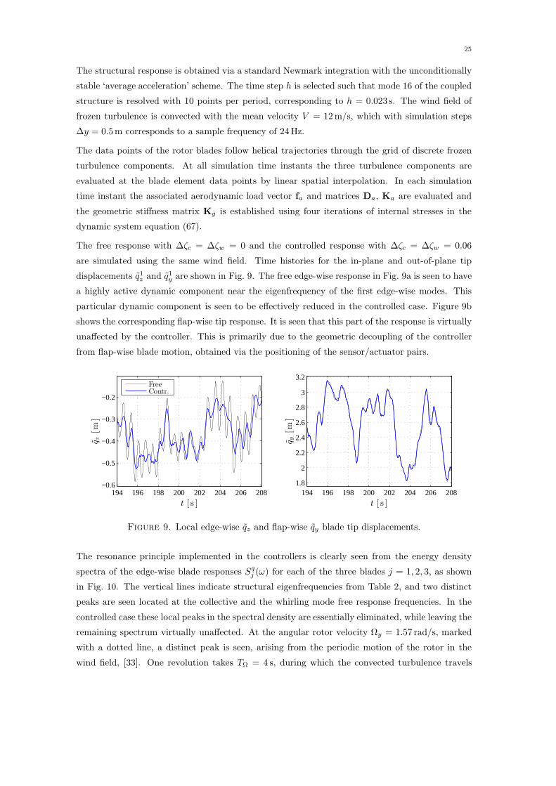
25
The structural response is obtained via a standard Newmark integration with the unconditionally
stable ‘average acceleration’ scheme. The time step ℎ is selected such that mode 16 of the coupled
structure is resolved with 10 points per period, corresponding to ℎ = 0.023 s. The wind field of
frozen turbulence is convected with the mean velocity 𝑉 = 12m/s, which with simulation steps
Δ𝑦 = 0.5m corresponds to a sample frequency of 24Hz.
The data points of the rotor blades follow helical trajectories through the grid of discrete frozen
turbulence components. At all simulation time instants the three turbulence components are
evaluated at the blade element data points by linear spatial interpolation. In each simulation
time instant the associated aerodynamic load vector f𝑎 and matrices D𝑎, K𝑎 are evaluated and
the geometric stiffness matrix K𝑔 is established using four iterations of internal stresses in the
dynamic system equation (67).
The free response with Δ𝜁𝑐 = Δ𝜁𝑤 = 0 and the controlled response with Δ𝜁𝑐 = Δ𝜁𝑤 = 0.06
are simulated using the same wind field. Time histories for the in-plane and out-of-plane tip
displacements 𝑞1𝑧 and 𝑞1𝑦 are shown in Fig. 9. The free edge-wise response in Fig. 9a is seen to have
a highly active dynamic component near the eigenfrequency of the first edge-wise modes. This
particular dynamic component is seen to be effectively reduced in the controlled case. Figure 9b
shows the corresponding flap-wise tip response. It is seen that this part of the response is virtually
unaffected by the controller. This is primarily due to the geometric decoupling of the controller
from flap-wise blade motion, obtained via the positioning of the sensor/actuator pairs.
194 196 198 200 202 204 206 208−0.6
−0.5
−0.4
−0.3
−0.2
FreeContr.
194 196 198 200 202 204 206 2081.8
2
2.2
2.4
2.6
2.8
3
3.2
𝑡 [ s ]𝑡 [ s ]
𝑞 𝑧[m
]
𝑞 𝑦[m
]
Figure 9. Local edge-wise 𝑞𝑧 and flap-wise 𝑞𝑦 blade tip displacements.
The resonance principle implemented in the controllers is clearly seen from the energy density
spectra of the edge-wise blade responses 𝑆𝑞𝑗 (𝜔) for each of the three blades 𝑗 = 1, 2, 3, as shown
in Fig. 10. The vertical lines indicate structural eigenfrequencies from Table 2, and two distinct
peaks are seen located at the collective and the whirling mode free response frequencies. In the
controlled case these local peaks in the spectral density are essentially eliminated, while leaving the
remaining spectrum virtually unaffected. At the angular rotor velocity Ω𝑦 = 1.57 rad/s, marked
with a dotted line, a distinct peak is seen, arising from the periodic motion of the rotor in the
wind field, [33]. One revolution takes 𝑇Ω = 4 s, during which the convected turbulence travels
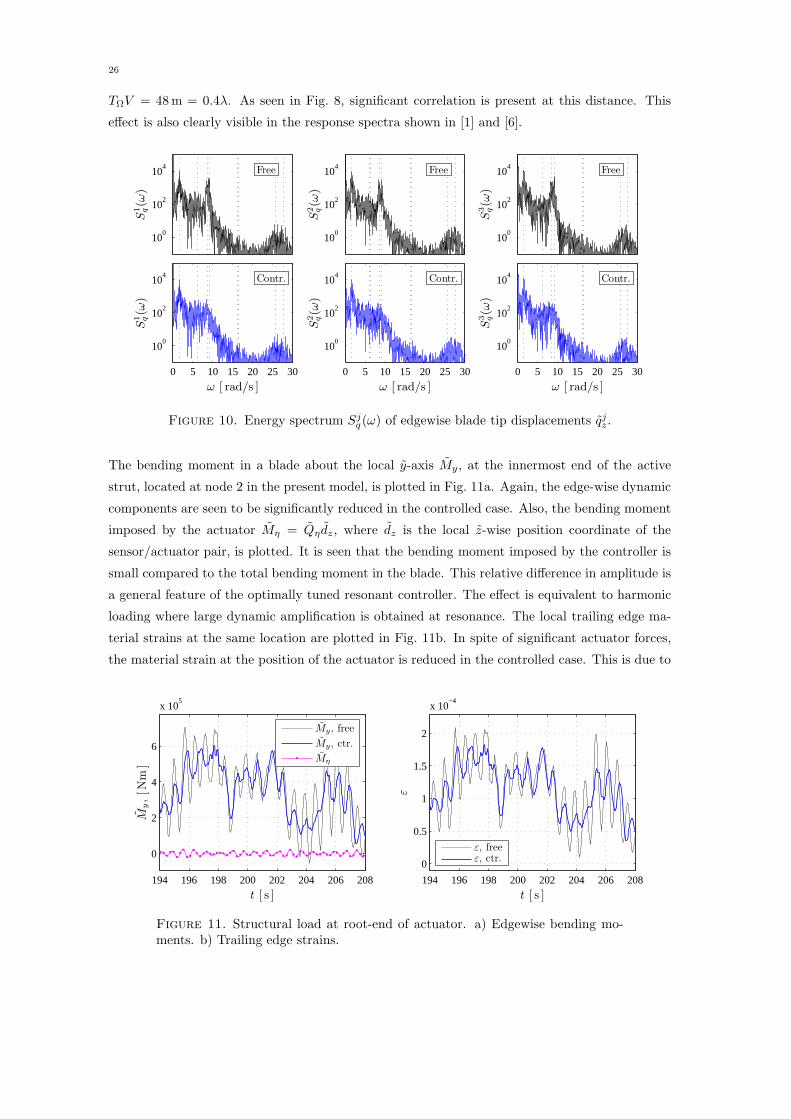
26
𝑇Ω𝑉 = 48m = 0.4𝜆. As seen in Fig. 8, significant correlation is present at this distance. This
effect is also clearly visible in the response spectra shown in [1] and [6].
100
102
104 Free
100
102
104 Free
100
102
104 Free
0 5 10 15 20 25 30
100
102
104 Contr.
0 5 10 15 20 25 30
100
102
104 Contr.
0 5 10 15 20 25 30
100
102
104 Contr.
𝜔 [ rad/s ]𝜔 [ rad/s ]𝜔 [ rad/s ]
𝑆1 𝑞(𝜔
)𝑆
1 𝑞(𝜔
)
𝑆2 𝑞(𝜔
)𝑆
2 𝑞(𝜔
)
𝑆3 𝑞(𝜔
)𝑆
3 𝑞(𝜔
)
Figure 10. Energy spectrum 𝑆𝑗𝑞(𝜔) of edgewise blade tip displacements 𝑞𝑗𝑧.
The bending moment in a blade about the local 𝑦-axis ��𝑦, at the innermost end of the active
strut, located at node 2 in the present model, is plotted in Fig. 11a. Again, the edge-wise dynamic
components are seen to be significantly reduced in the controlled case. Also, the bending moment
imposed by the actuator ��𝜂 = ��𝜂𝑑𝑧, where 𝑑𝑧 is the local 𝑧-wise position coordinate of the
sensor/actuator pair, is plotted. It is seen that the bending moment imposed by the controller is
small compared to the total bending moment in the blade. This relative difference in amplitude is
a general feature of the optimally tuned resonant controller. The effect is equivalent to harmonic
loading where large dynamic amplification is obtained at resonance. The local trailing edge ma-
terial strains at the same location are plotted in Fig. 11b. In spite of significant actuator forces,
the material strain at the position of the actuator is reduced in the controlled case. This is due to
194 196 198 200 202 204 206 208
0
2
4
6
x 105
My, free
My, ctr.
Mη
194 196 198 200 202 204 206 208
0
0.5
1
1.5
2
x 10−4
ε, freeε, ctr.
𝑡 [ s ]𝑡 [ s ]
𝑀𝑦,[N
m]
𝜀
Figure 11. Structural load at root-end of actuator. a) Edgewise bending mo-ments. b) Trailing edge strains.

27
the fact that the optimally tuned resonant controller deploys actuator force for maximal energy
dissipation. This occurs at peak velocities where structural displacements vanish.
Both forward and backward whirling produce hub reaction forces perpendicular to the axis of
rotation which must be balanced by the rotor shaft. To illustrate this effect the local blade root
shear forces measured in the rotor coordinate system 𝑄𝑥, 𝑄𝑧 are evaluated and the energy density
spectra 𝑆𝑥𝑄(𝜔), 𝑆𝑧𝑄(𝜔) of the resulting rotor hub forces 𝑄𝑥, 𝑄𝑧 are plotted in Fig. 12. In the free
response this load appears as distinct peaks at the first edge-wise whirling frequencies. As seen
from the controlled response the whirling controller effectively eliminates this component of the
energy spectrum.
106
108
1010
Free
106
108
1010
Free
0 5 10 15 20 25 3010
6
108
1010
Contr.
0 5 10 15 20 25 3010
6
108
1010
Contr.
𝜔 [ rad/s ]𝜔 [ rad/s ]
𝑆𝑥 𝑄(𝜔
)𝑆
𝑥 𝑄(𝜔
)
𝑆𝑧 𝑄(𝜔
)𝑆
𝑧 𝑄(𝜔
)
Figure 12. Energy density spectra 𝑆𝑥𝑄(𝜔), 𝑆𝑧𝑄(𝜔) of the rotor hub forces 𝑄𝑥 and 𝑄𝑧.
A typical design factor for linear actuator systems is the required stroke velocity. A sample of
the stroke velocity 𝑞𝜂 is shown in Fig. 13a. In the present case the stroke velocities range within
±4mm/s. The range of actuator forces𝑄𝜂 in the present application is ±60 kN. Both requirements
194 196 198 200 202 204 206 208−4
−2
0
2
4x 10
−3
194 196 198 200 202 204 206 208
−20
0
20
40
60
80
100
𝑡 [ s ]𝑡 [ s ]
𝑞 𝜂[m
/s]
𝑃𝜂,[W
]
Figure 13. Actuator displacement velocity 𝑞𝜂 and dissipative actuator power 𝑃𝜂.

28
are easily met by existing hydraulic actuators, and this technology is already widely used in the
active pitch regulation systems of modern wind turbines.
The dissipative power of an actuator 𝑃𝜂 = 𝑄𝜂𝑞𝜂 is shown in Fig. 13. Occasional negative contri-
butions are seen to occur, however the energy dissipation is generally positive. The continuous
power consumption of the controller is in the range of 100 W which is insignificant compared to
the mega-Watt power production capacity of modern wind turbines.
6. Conclusions
It has been known for the last decade that edge-wise vibrations of the blades in three-bladed rotors
for wind turbines are potentially very lightly damped. These vibration modes occur in groups of
three due to the three-fold symmetry of the rotor, and a method for control of such a group of
vibration modes has been developed. The method makes use of collocated control via a single
active strut with sensor/actuator capacity in each of the three blades. The controller system is
based on the concept of resonance, generalizing the idea of the tuned mass damper. Thus, the
combined information from the sensor in each of the three blades must be used to extract the
relevant information about the current magnitude of the targeted modal response. When using
the minimum number of sensor/actuator pairs – here three active struts for the group of three
associated edge-wise vibration modes – it is unavoidable that the response also contains non-
resonant contributions from other modes. The procedure developed here separates the response
into that of the collective mode of the group, and the combined response from the pair of whirling
modes in the group. For each of these two types of response a quasi-static correction is developed
to account for the extra flexibility created by the non-resonant part of the response. In typical
three-bladed wind turbine rotors the sensor/actuator struts can be mounted such that the effect
is orthogonal or nearly orthogonal to the relevant group(s) of flap-wise vibration modes. Low-
frequency tower modes will typically be separated frequency-wise from the targeted edge-wise
vibration modes, and the quasi-static correction terms can therefore be expressed explicitly in
terms of the stiffness matrix and the mode-shapes of the targeted modes, without need for a
complete modal analysis of the system.
The calibration procedure makes use of a full eigenvalue analysis of the rotating blades with
complex-valued mode-shapes. The full modal expansion in this case has 2𝑁 terms, each associated
with a frequency factor (𝜔𝑗 ± 𝜔)−1, instead of the eigenvalue problem for non-rotating systems
with an 𝑁 -term solution with frequency factors (𝜔2𝑗 −𝜔2)−1. It is demonstrated, how the general
complex formulation can be used in an approximate form, that appears as a simple introduction
of complex mode-shape vectors in the classic form for non-rotating structures. The resulting
formulation is in terms of real-valued coefficients, permitting use of the optimal parameter formulae
for non-rotating structures.
The performance of the resonant control procedure with three active struts has been investigated
in relation to a wind turbine rotor with a diameter of 86 m, representative of current large-size

29
wind turbines. The analysis demonstrates as illustrated in Fig. 6 that the controller calibration
is close to optimal, when the quasi-static correction is included, while omission of the effect of
the additional quasi-static flexibility will result in a rather unbalanced calibration with reduced
damping capacity. The introduction of a quasi-static correction leads to a controller format that
is more general than that associated with a tuned mass absorber. While the tuned mass absorber
is a purely passive device, the use of the generalized format may lead to a need for an active power
supply as illustrated in Fig. 13b. However, the necessary power capacity is quite low compared
to the dissipated power. The idea of the resonant control is to target one or more selected
modes specifically, with the expectation that this will reduce oscillations occurring at the targeted
frequencies. The effectiveness is clearly illustrated in the response records shown in Figs. 9 and 11.
Thus, the resonant damping approach appears very suitable for reduction of the fatigue loading
on wind turbine rotor blades. The use of a local active strut introduces local structural loads,
but the records shown in Fig. 11 indicate that the local controller loads are modest relative to the
effect of the direct structural loads.
Appendix A. Wind Field Simulation
A.1. Isotropic wind field
The turbulent wind field used in the present paper is represented in the form of isotropic incom-
pressible turbulence as described by Batchelor [31]. The general form of the covariance between
the turbulent velocity components at two points separated by the spatial vector x then is
R(r) = E[v(r0 + r)v(r0)𝑇 ] = 𝜎2𝑣
(
[ 𝑓(𝑟) − 𝑔(𝑟) ]r r𝑇
r𝑇 r+ 𝑔(𝑟)
)
, (A.1)
where 𝑟 = ∣r∣ is the distance between the two points, and 𝜎2𝑣 is the variance of a single component
at a point. 𝑓(𝑟) and 𝑔(𝑟) are the lengthwise and transverse correlation function, respectively. It
follows from incompressibility that they are related by
𝑔(𝑟) = 𝑓(𝑟) +𝑟
2
𝑑
𝑑𝑟𝑓(𝑟). (A.2)
The covariance functions are described by the lengthwise spectral density function 𝐹 (𝑘), where 𝑘
is the wavenumber,
𝜎2𝑣𝑓(𝑟) =
∫
∞
−∞
𝐹 (𝑘) e𝑖𝑘𝑟𝑑𝑟. (A.3)
Analytically tractable results are obtained when using the von Karman spectral density, [32],
𝜎2𝑣𝐹 (𝑘) =
1√𝜋
Γ(𝛾)
Γ(𝛾 − 12 )
𝜎2𝑢 ℓ
[ 1 + (𝑘ℓ)2]𝛾. (A.4)
The Kolmogorov cascade theory implies that the exponent is 𝛾 = 5/6. In this case the covariance
functions can be expressed in terms of Airy functions [34], when introducing the non-linear variable
transformation
𝑧 =(3𝑟
2ℓ
)2/3
, (A.5)
whereby
𝑓(𝑟) =Ai(𝑧)
Ai(0), 𝑔(𝑟) = 𝑓(𝑟) +
𝑧
3
Ai′(𝑧)
Ai(0). (A.6)

30
Here Ai(𝑧) is the Airy function and Ai′(𝑧) its derivative. A simpler approximate formulation is
obtained by using 𝛾 = 1, whereby
𝑓(𝑟) = e−𝑟/𝜆, 𝑔(𝑟) =(
1 − 1
2
𝑟
𝜆
)
e−𝑟/𝜆. (A.7)
In this formulation 𝜆 is the integral spatial length-scale. When using the same integral length-scale
in (A.6) it follows that ℓ = 1.339𝜆. The Airy and exponential formats are compared in Fig. A.1,
showing that the curves cross at 𝑟 ≃ 𝜆.
0 1 2 3 4−0.2
0
0.2
0.4
0.6
0.8
1
1.2fe(r)fa(r)
0 1 2 3 4−0.2
0
0.2
0.4
0.6
0.8
1
1.2ge(r)ga(r)
𝑓(𝑟
)
𝑔(𝑟
)
𝑟/𝜆𝑟/𝜆
Figure A.1. Correlation functions 𝑓(𝑟) and 𝑔(𝑟): Airy (dots), Exponential (full).
A.2. Autoregressive simulation
In the present context, where the main purpose is to estimate the reduction of the resonant
response, the turbulent wind field is simulated by use of an autoregressive model represented by
the single-step recurrence relation
v𝑛 = Av𝑛−1 + B𝝃𝑛−1, 𝑛 = 1, 2, ⋅ ⋅ ⋅ (A.8)
The array v𝑛 contains the wind components at a chosen number of points in a transverse plane
relative to the average wind, and 𝝃𝑛 contains corresponding uncorrelated normally distributed
variables,
v𝑛 = [ 𝑣1, 𝑣2, ⋅ ⋅ ⋅ , 𝑣𝑚 ]𝑇𝑛 , 𝝃𝑛 = [ 𝜉1, 𝜉2, ⋅ ⋅ ⋅ , 𝜉𝑚 ]𝑇𝑛 (A.9)
The subscript 𝑛 denotes the time 𝑡𝑛 = 𝑛Δ𝑡, and each step in the recurrence corresponds to a time
increment Δ𝑡. The relation between spatial coordinates and time is provided by the mean wind
speed 𝑉 via the hypothesis of convected ‘frozen turbulence’, [31]. Hereby the time increment Δ𝑡
corresponds to the downwind distance
Δ𝑦 = 𝑉 Δ𝑡 , (A.10)
and time separation can be related to the spatial covariance function (A.1).
The chief advantage of the simple single-step algorithm (A.8) is the simple relation between the
matrices A, B and the covariance function describing the field,
R𝑗 = E[v𝑛v𝑇𝑛−𝑗 ] 𝑗 = ⋅ ⋅ ⋅ ,−1, 0, 1, ⋅ ⋅ ⋅ . (A.11)

31
Although the single-step autoregressive model imposes severe constraints on the simulated field,
it appears to capture the essential properties of the present problem sufficiently well.
For calibration over a single step the matrices A and B can be identified directly via conditional
expected values in the stochastic wind field. The idea is to consider v𝑛−1 known. Hereby the
conditional expectation of v𝑛 becomes
E[v𝑛∣v𝑛−1] = Av𝑛−1. (A.12)
Thus, A is identified as the matrix in the conditional mean formula of a set of correlated stochastic
variables, given by
A = R1R−10 . (A.13)
The matrix B is determined by collecting the two response terms on the left side of the equation,
v𝑛 − Av𝑛−1 = B𝝃𝑛−1. (A.14)
Both sides represent a normal vector variable with zero mean. When the vector v𝑛−1 is assumed
known, the covariance matrix of the right hand side corresponds to the conditional covariance
of v𝑛,
Cov[v𝑛v𝑇𝑛 ∣v𝑛−1] = BE[ 𝝃𝑛−1𝝃
𝑇𝑛−1]B
𝑇 . (A.15)
The vector 𝝃𝑛−1 has independent normalized components, and thus the product BB𝑇 is the
conditional covariance
BB𝑇 = Cov[v𝑛v𝑇𝑛 ∣v𝑛−1] = R0 − R1R
−10 R𝑇
1 , (A.16)
It is observed that the two parameter matrices of the AR filter are determined by the conditional
expectation and the conditional covariance with the previous variable v𝑛−1 known.
References
[1] Hansen, M.O.L., Sørensen, J.N., Voutsinas, S., Sørensen, S., and Madsen, H.Aa., State of the art in wind
turbine aerodynamics and aeroelasticity, Progress in Aerospace Sciences, Vol. 42, 2006, pp. 285–330.
[2] Friedmann, P.P., Rotary-wing aeroelasticity: Current status and future trends, AIAA Journal, Vol. 42, 2004,
pp. 1953–1972.
[3] Thomsen, K., Petersen, J.T., Nim, E., Øye, S., and Petersen, B., A method for determination of damping for
edgewise blade vibrations, Wind Energy, Vol. 3, 2000, pp. 233–246.
[4] Hansen, M.H., Improved modal dynamics of wind turbines to avoid stall-induced vibrations, Wind Energy,
Vol. 6, 2003, pp. 179–195.
[5] Riziotis, V.A., Voutsinas, S.G., Politis, E.S., and Chaviaropoulos, P.K., Aeroelastic stability of wind turbines:
the problem, the methods and the issues, Wind Energy, Vol. 7, 2004, pp. 373–392.
[6] Hansen, M.H., Thomsen, K., Fuglsang, P., and Knudsen, T., Two methods for estimating aeroelastic damping
of operational wind turbine modes from experiments, Wind Energy, Vol. 9, 2006, pp. 179–191.
[7] Meirovitch, L., Dynamics and Control of Structures, Wiley, New York, 1990.
[8] Khulief, Y.A., Vibration suppression in rotating beams using active modal control, Journal of Sound and
Vibration, Vol. 242, 2001, pp. 681–699.
[9] Chandiramani, N.K., Librescu, Saxena V., L.I., and Kumar, A., Optimal vibration control of a rotating
composite beam with distributed piezoelectric sensing and actuation, Smart Materials and Structures, Vol. 13,
2004, pp. 433–442.
32
[10] Shete, C.D., Chandiramani, N.K., and Librescu, L.I., Optimal control of a pretwisted shearable smart com-
posite rotating beam, Acta Mechanica, Vol. 191, 2007, pp. 37–58.
[11] Rice, J.K., and Verhaegen, M., Robust and distributed control of a smart blade, Wind Energy, Vol. 13, 2010,
pp. 103–116.
[12] Barlas, T.K., and van Kuik, G.A.M., Review of state of the art in smart rotor control research for wind
turbines, Progress in Aerospace Sciences, Vol. 46, 2010, pp. 1–27.
[13] Buhl, T., Gaunaa, M., and Bak, C., Potential load reduction using airfoils with variable trailing edge geometry,
Journal of Solar Energy Engineering, Vol. 127, 2005, pp. 503–516.
[14] Andersen, P.B., Henriksen, L., Gaunaa, M., Bak, C., and Buhl, T., Deformable trailing edge flaps for modern
megawatt wind turbine controllers using strain gauge sensors, Wind Energy, Vol. 13, 2010, pp. 193–206.
[15] Krenk, S., and Høgsberg, J., Optimal resonant control of flexible structures, Journal of Sound and Vibration,
Vol. 323, 2009, pp. 530–554.
[16] Krenk, S., and Høgsberg, J., Resonant damping of flexible structures under random excitation, in Compu-
tational Methods in Stochastic Dynamics, eds. Papadrakakis, M., et al., Computational Methods in Applied
Sciences, vol. 22, Springer, Dordrecht, 2011, pp., 25–46. (DOI 10.1007/978-90-481-9987-7 2)
[17] Coleman, R.P., Theory of self-excited mechanical oscillations of hinged rotor blades, Technical Report NACA-
WR-L-308, Langley Research Center, 1943. (http://ntrs.nasa.gov).
[18] Thomas, D.L., Dynamics of rotationally periodic structures, International Journal for Numerical Methods in
Engineering, Vol. 14, 1979, pp. 81–102.
[19] Kosmatka, J.B. and Friedmann, P.P., Vibration analysis of composite turbopropellers using a non-liear beam-
type finite-element approach, AIAA Journal, Vol. 27, 1989, pp. 1606–1614.
[20] Geradin, and M., Rixen, D., Mechanical Vibrations, second ed., Wiley, Chichester, 1997.
[21] Svendsen, M.N., Krenk, K., and Høgsberg, J., Resonant vibration control of rotating beams, Journal of Sound
and Vibration, 2010. (doi:10.1016/j.jsv.2010.11.008)
[22] Meirovitch, L., A new method of solution of the eigenvalue problem for gyroscopic systems, AIAA Journal,
Vol. 12, 1974, pp. 1337–1342.
[23] Meirovitch, L., Principles and Techniques of Vibrations, Prentice-Hall, Upper Saddle River, New Jersey, 1997.
[24] Krenk, S., and Nielsen, M.B., Hybrid state-space time integration in a rotating frame of reference. Department
of Mechanical Engineering, Technical University of Denmark, 2010. (to be published)
[25] Hansteen, O.E., and Bell, K., Accuracy of mode superposition analysis in structural dynamics, Earthquake
Engineering and Structural Dynamics, Vol. 7, 1979, pp. 405–411.
[26] Den Hartog, J.P., Mechanical Vibrations, 4th ed. McGraw-Hill, New York, 1956. (Reprinted by Dover, New
York, 1985.)
[27] Krenk, S., Frequency analysis of the tuned mass damper, Journal of Applied Mechanics, Vol. 72, 2005, pp.
936–942.
[28] Preumont, A., Vibration Control of Active Structures, An Introduction, 2nd edition, Kluwer, Dordrecht, 2002.
[29] Svendsen, M.N., Krenk, S., and Høgsberg, J., Resonant vibration control of wind turbine blades, Torque 2010:
The Science of Making Torque from Wind, June 28-30, Crete, Greece, 2010, pp. 543–553.
[30] Krenk, S., and Høgsberg, J., Tuned mass absorbers on damped structures under random load, Probabilistic
Engineering Mechanics, Vol. 23, 2008, pp. 408–415.
[31] Batchelor, G.K., The Theory of Homogeneous Turbulence, Cambridge University Press, Cambridge, UK, 1953.
[32] von Karman, T., Progres in the statistical theory of turbulence, Proceedings of the National Academy of
Science, Vol. 34, 1948, pp. 530–539.
[33] Kristensen, L., and Frandsen, S., Model for power spectra of the blade of a wind turbine measured from the
moving frame of reference, Journal of Wind Engineering and Industrial Aerodynamics, Vol. 10, 1982, pp.
249–262.
[34] Olver, F.W.J., Lozier, D.W., Boisvert, R.F., and Clark, C.W., NIST Handbook of Mathematical Functions,
Cambridge University Press, Cambridge, UK, 2010.


DTU Mechanical Engineering
Section of Coastal, Maritime and Structural Engineering
Technical University of Denmark
Nils Koppels Allé, Bld. 403
DK- 2800 Kgs. Lyngby
Denmark
Phone (+45) 45 25 13 60
Fax (+45) 45 88 43 25
www.mek.dtu.dk
ISBN: 978-87-90416-42-3
DCAMM
Danish Center for Applied Mathematics and Mechanics
Nils Koppels Allé, Bld. 404
DK-2800 Kgs. Lyngby
Denmark
Phone (+45) 4525 4250
Fax (+45) 4593 1475
www.dcamm.dk
ISSN: 0903-1685