wolf and lam
DESCRIPTION
A loop transformation and algorithm to maximize parallelismTRANSCRIPT

A Loop Transformation Theory and
an Algorithm to Maximize Parallelismyz
Michael E. Wolf and Monica S. LamComputer Systems LaboratoryStanford University, CA 94305
Abstract
This paper proposes a new approach to transformations for general loop nests. In this approach, we unify all
combinations of loop interchange, skewing and reversal as unimodular transformations. The use of matrices to
model transformations has previously been applied only to those loop nests whose dependences can be summarized
by distance vectors. Our technique is applicable to general loop nests where the dependences include both distances
and directions.
This theory provides the foundation for solving an open question in compilation for parallel machines: Which
loop transformations, and in what order, should be applied to achieve a particular goal, such as maximizing
parallelism or data locality. This paper presents an efficient loop transformation algorithm based on this theory to
maximize the degree of parallelism in a loop nest.
1 Introduction
Loop transformations, such as interchange, reversal, skewing and tiling (or blocking) [1, 4, 26] have been shown to
be useful for two important goals: parallelism and efficient use of the memory hierarchy. Existing vectorizing and
parallelizing compilers focused on the application ofindividual transformations on pairs of loops: when it is legal
to apply a transformation, and if the transformation directly contributes to a particular goal. However, the more
challenging problems of generating code for massively parallel machines, or improving data locality, require the
application of compound transformations. It remains an open question as to how to combine these transformations to
optimize general loop nests for a particular goal. This paper introduces a theory of loop transformations that offers
an answer to this question. We will demonstrate the use of this theory with an efficient algorithm that maximizes
the degrees of both fine- and coarse-grain parallelism in a set of loop nests via compound transformations.
Existing vectorizing and parallelizing compilers implement compound transformations as a series of pairwise
transformations; for each step, the compiler must choose a transform that is legal and desirable to apply. A technique
y A preliminary version of this paper appeared inThe 3rd Workshop on Programming Languages and Compilers for Parallel Computing, Aug.
1990, Irvine CA.
z This research was supported in part by DARPA contract N00014-87-K-0828.
1

commonly used in today’s parallelizing compilers is to decidea priori the order in which the compiler should attempt
to apply transformations. This technique is inadequate because the choice and ordering of optimizations are highly
program dependent, and the desirability of a transform cannot be evaluated locally, one step at a time. Another
proposed technique is to “generate and test”, that is, to explore all different possible combinations of transformations.
This “generate and test” approach is expensive. Differently transformed versions of the same program may trivially
have the same behavior and so need not be explored. For example, when vectorizing, the order of the outer loops
is not significant. More importantly, generate and test approaches cannot search the entire space of transformations
that have potentially infinite instantiations. Including loop skewing in a “generate and test” framework is thus
problematic, because a wavefront can travel in an infinite number of different directions.
An alternative approach, based on matrix transformations, has been proposed and used for an important subset
of loop nests. This class includes many important linear algebra codes on dense matrices; all systolic array
algorithms belong to this class. They have the characteristic that their dependences can be represented by a set of
integer vectors, known asdistance vectors. Loop interchange, reversal, and skewing transformations are modeled
as unimodular transformations in the iteration space [7, 8, 12, 13, 19, 21]. A compound transformation is just
another linear transformation, being a product of several elementary transformations. This model makes it possible
to determine the compound transformation directly in maximizing some objective function. Loop nests whose
dependences can be represented as distance vectors have the property that ann-deep loop nest has at leastn � 1
degrees of parallelism [13], and can exploit data locality in all possible loop dimensions [24]. Distance vectors
cannot represent the dependences of general loop nests, where two or more loops must execute sequentially. A
commonly used notation for representing general dependences isdirection vectors[2, 26].
This research combines the advantages of both approaches. We combine the mathematical rigor in the matrix
transformation model with the generality of the vectorizing and concurrentizing compiler approach. We unify
the various transformations, interchange or permutation, reversal and skewing as unimodular transformations, and
our dependence vectors incorporate both distance and direction information. This unification provides a general
condition to determine if the code obtained via a compound transformation is legal, as opposed to a specific legality
test for each individual elementary transformation. Thus the loop transformation problem can be formulated as
directly solving for the transformation that maximizes some objective function, while satisfying a set of constraints.
One important consequence of this approach is that code and loop bounds can be transformed once and for all,
given the compound transformation.
Using this theory, we have developed algorithms for improving the parallelism and locality of a loop nest via
loop transformations. Our parallelizing algorithm maximizes the degree of parallelism, the number of parallel loops,
within a loop nest. By finding the maximum number of parallel loops, multiple consecutive loops can be coalesced
to form a single loop with all the iterations; this facilitates load balancing and reduces synchronization overhead.
Especially for loops with a small number of loop iterations, parallelizing only one loop may not fully exploit all
the parallelism in the machine. The algorithm can generate coarse-grain and/or fine-grain parallelism; the former
is useful in multiprocessor organizations and the latter is useful for vector machines and superscalar machines,
machines that can execute multiple instructions per cycle. It can also generate code for machines that can use
multiple levels of parallelism, such as a multiprocessor with vector nodes.
2

We have also applied our representation of transformations successfully to the problem of data locality. All
modern machine organizations, including uniprocessors, employ a memory hierarchy to speed up data accesses;
the memory hierarchy typically consists of registers, caches, primary memory and secondary memory. As the
processor speed improves and the gap between processor and memory speeds widens, data locality becomes more
important. Even with very simple machine models (for example, uniprocessors with data caches), complex loop
transformations may be necessary [9, 10, 17]. The consideration of data locality makes it more important to be able
to combine primitive loop transformations in a systematic manner. Using the same theoretical framework presented
in this paper, we have developed a locality optimization that applies compound unimodular loop transforms and
tiling to use the memory hierarchy efficiently [24].
This paper introduces our model of loop dependences and transformations. We describe how the model facilitates
the application of compound transformation, using parallelism as our target. The model is important in that it enables
the choice of an optimal transformation without an exhaustive search. The derivation of the optimal compound
transformation consists of two steps. The first step puts the loops into a canonical form, and the second step tailors
it to specific architectures. While the first step can be expensive in the worst case, we have developed an algorithm
that is feasible in practice. We apply a cheaper technique to handle as many loops as possible, and use the more
general and expensive technique only on the remaining loops. For most loop nests, the algorithm finds the optimal
transformation inO(n
3d) time, wheren is the depth of the loop nests andd is the number of dependence vectors.
The second step of specializing the code for different granularities of parallelism is straightforward and efficient.
After deciding on the compound transformation to apply, the code including the loop bounds is then modified.
The loop transformation algorithm has been implemented in our SUIF (Stanford University Intermediate Format)
parallelizing compiler. As we will show in the paper, the algorithms are simple, yet powerful.
This paper is organized as follows: We introduce the concept of our loop transformation model by first discussing
the simpler program domain where all dependences are distance vectors. We first describe the model and present
the parallelization algorithm. After extending the representation to directions, we describe the overall algorithm and
the specific heuristics used. Finally we describe a method for rewriting the loop body and bounds after a compound
transformation.
2 Loop Transformations on Distance Vectors
In this section, we introduce our basic approach to loop transformations by first studying the narrower domain of
loops whose dependences can be represented as distance vectors. The approach has been adopted by numerous
researchers particularly in the context of automatic systolic algorithm generation, a discussion of which can be
found in Ribas’ dissertation [20].
2.1 Loop Nest Representation
In this model, a loop nest of depthn is represented as a finite convex polyhedron in the iteration spaceZ
n
bounded by the loop bounds. Each iteration in the loop corresponds to a node in the polyhedron, and is identified by
3

(a)
for I1 := 0 to 5 do
for I2 := 0 to 6 do
a[I2 + 1] := 1/3 * (a[I2] + a[I2 + 1] + a[I2 + 2]);
D = f(0; 1); (1;0); (1;�1)g.
I
0
I
0
I
0
I
0
I
0
� I
0
+ I
0
� I
0
I
0
� I
0
+ I
0
� I
0
+
T =
� �
D
0
= TD = f( ; ); ( ; ); ( ; )g

its index vector~p = (p1; p2; . . . ; pn
)
1; pi
is the value of theith loop index in the nest, counting from the outermost
to innermost loop. In a sequential loop, the iterations are therefore executed in lexicographic order of their index
vectors.
The execution order of the iterations is constrained by their data dependences. Scheduling constraints for many
numerical codes are regular and can be succinctly represented bydependence vectors. A dependence vector in an
n-nested loop is denoted by a vector~d= (d1; d2; . . . ; d
n
). The discussion in this section is limited todistance
vectors, that is,di
2 Z. Techniques for extracting distance vectors are discussed in [12, 16, 22]. General loop
dependences may not be representable with a finite set of distance vectors; extensions to include directions are
necessary and will be discussed in Section 4.
Each dependence vector defines a set of edges on pairs of nodes in the iteration space. Iteration~p1 must execute
before ~p2 if for some distance vector~d, ~p2 = ~p1 +
~
d. The dependence vectors define a partial order on the nodes
in the iteration space, and any topological ordering on the graph is a legal execution order, as all dependences in
the loop are satisfied. In a sequential loop nest, the nodes are executed in lexicographic order, thus dependences
extracted from such a source program can always be represented as a set oflexicographically positivevectors. A
vector~d
is lexicographically positive, written~d�
~0, if 9i :�
d
i
> 0 and8j < i : dj
� 0�
. (~0 denotes a zero vector,
that is, a vector with all components equal to 0.)
Figure 1(a) shows an example of a loop nest and its iteration space representation. Each axis represents a
loop; each node represents an iteration that is executed within the loop nest. The 42 iterations of the loop are
represented as a 6� 7 rectangle in the 2-dimensional space. Finally, each arrow represents a scheduling constraint.
The accessa[I2] refers to data generated by the previous iteration from the same innermost loop, whereas the
remaining two read accesses refer to data from the previous iteration of the outer loop. The dependence edges are
all lexicographically positive:f(0; 1); (1; 0); (1;�1)g.
2.2 Unimodular Transformations
It is well known that loop transformations such as interchange, reversal, and skewing are useful in parallelization or
improving the efficiency of the memory hierarchy. These loop transformations can be modeled as elementary matrix
transformations; combinations of these transformations can simply be represented as products of the elementary
transformation matrices. The optimization problem is thus to find the transformation that maximizes an objective
function given a set of scheduling constraints.
We use the loop interchange transformation to illustrate the transformation model. A loop interchange transfor-
1The dependence vector~d
is a column vector. In this paper we sometimes represent column vectors as comma-separated tuples. That is,
(p1; p2; . . . ; pn
) =
�
p1 p2 . . . p
n
�
T
=
2
6
4
p1p2
...p
n
3
7
5
:
5

mation maps iteration(i; j) to iteration(j; i). In matrix notation, we can write this as�
0 11 0
� �
i
j
�
=
�
j
i
�
:
The elementary permutation matrix
�
0 11 0
�
thus performs the loop interchange transformation on the iteration
space.
To understand how dependences are mapped byT , suppose there is a dependence from iteration~p1 to ~p2. Since
a matrixT performs a linear transformation on the iteration space,T~p2 � T~p1 = T (~p2 � ~p1). Therefore, if~d
is a
distance vector in the original iteration space, thenT
~
dis a distance vector in the transformed iteration space. Thus
in loop interchange, the dependence vector(d1; d2) is mapped into�
0 11 0
��
d1
d2
�
=
�
d2
d1
�
in the transformed space.
There are three elementary transformations:
� Permutation: A permutation� on a loop nest transforms iteration(p 1; . . . ; pn
) to (p
�1 ; . . . ; p�
n
). This
transformation can be expressed in matrix form asI
�
, then� n identity matrixI with rows permuted by�.
The loop interchange above is ann = 2 example of the general permutation transformation.
� Reversal:Reversal ofith loop is represented by the identity matrix, but with theith diagonal element equal
to �1 rather than 1. For example, the matrix representing loop reversal of the outermost loop of a two-deep
loop nest is
�
�1 00 1
�
.
� Skewing:Skewing loopIj
by an integer factorf with respect to loopIi
[26] maps iteration
(p1; . . . ; pi�1; pi; pi+1; . . . ; p
j�1; pj; pj+1; . . . ; pn
)
to
(p1; . . . ; pi�1; pi; pi+1; . . . ; p
j�1; pj + fp
i
; p
j+1; . . . ; pn
):
The transformation matrixT that produces skewing is the identity matrix, but with the elementt
j;i
equal tof
rather than zero. Sincei < j, T must be lower triangular. For example, the transformation from Figure 1(a)
to Figure 1(b) is a skew of the inner loop with respect to the outer loop by a factor of one, which can be
represented as
�
1 01 1
�
.
All these elementary transformation matrices are unimodular matrices [3]. A unimodular matrix has three
important properties. First, it is square, meaning that it maps ann-dimensional iteration space to ann-dimensional
iteration space. Second, it has all integral components, so it maps integer vectors to integer vectors. Third, the
absolute value of its determinant is one. Because of these properties, the product of two unimodular matrices
is unimodular, and the inverse of a unimodular matrix is unimodular, so that combinations of unimodular loop
transformations and inverses of unimodular loop transformations are also unimodular loop transformations.
6

A compound transformation can be synthesized from a sequence of primitive transformations, and the effect
of the transformation is represented by the products of the various transformation matrices for each primitive
transformation.
2.3 Legality of Unimodular Transformations
We say that it islegal to apply a transformation to a loop nest if the transformed code can be executed sequentially,
or in lexicographic order of the iteration space. We observe that if nodes in the transformed code are executed in
lexicographic order, all data dependences are satisfied if the transformed dependence vectors are lexicographically
positive. This observation leads to a general definition of a legal transformation and a theorem for legality of a
unimodular transformation.
Definition 2.1 A loop transformation islegal if the transformed dependence vectors are all lexicographically
positive.
Theorem 2.1 . LetD be the set of distance vectors of a loop nest. A unimodular transformationT is legal if and
only if 8~d2 D : T~
d�
~0.
Using this theorem, we can evaluate if a compound transformation is legal directly. Consider the following
example:
for I1 := 1 to N do
for I2 := 1 to N do
a[I1,I2] := f(a[I1,I2],a[I1 + 1,I2 � 1]);
end for
end for
This code has the dependence(1;�1). The loop interchange transformation, represented by
T =
�
0 11 0
�
;
is illegal, sinceT (1;�1) = (�1; 1) is lexicographically negative. However, compounding the interchange with a
reversal, represented by the transformation
T
0
=
�
�1 00 1
� �
0 11 0
�
=
�
0 �11 0
�
is legal sinceT 0
(1;�1) = (1; 1) is lexicographically positive.
Similarly, Theorem 2.1 also helps to deduce the set of legal compound transformations. For example, ifT is
lower triangular with unit diagonals (loop skewing) then a legal loop nest will remain so after transformation.. For
another example, consider the dependences of the loop nest in Figure 1(b). All the components of the dependences
are non-negative. This implies that any arbitrary loop permutation would render the transformed dependences
lexicographically positive and is thus legal. We say such loop nests arefully permutable. Full permutability is an
important property both for parallelization, discussed below, and for locality optimizations [24].
7
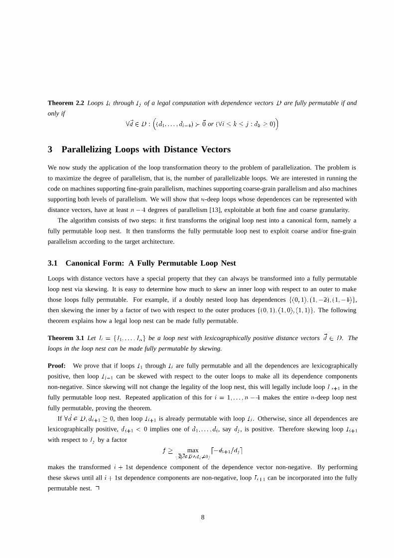
Theorem 2.2 LoopsIi
throughIj
of a legal computation with dependence vectorsD are fully permutable if and
only if
8
~
d2 D :
�
(d1; . . . ; di�1) � ~0 or (8i � k � j : d
k
� 0)�
3 Parallelizing Loops with Distance Vectors
We now study the application of the loop transformation theory to the problem of parallelization. The problem is
to maximize the degree of parallelism, that is, the number of parallelizable loops. We are interested in running the
code on machines supporting fine-grain parallelism, machines supporting coarse-grain parallelism and also machines
supporting both levels of parallelism. We will show thatn-deep loops whose dependences can be represented with
distance vectors, have at leastn� 1 degrees of parallelism [13], exploitable at both fine and coarse granularity.
The algorithm consists of two steps: it first transforms the original loop nest into a canonical form, namely a
fully permutable loop nest. It then transforms the fully permutable loop nest to exploit coarse and/or fine-grain
parallelism according to the target architecture.
3.1 Canonical Form: A Fully Permutable Loop Nest
Loops with distance vectors have a special property that they can always be transformed into a fully permutable
loop nest via skewing. It is easy to determine how much to skew an inner loop with respect to an outer to make
those loops fully permutable. For example, if a doubly nested loop has dependencesf(0; 1); (1;�2); (1;�1)g,
then skewing the inner by a factor of two with respect to the outer producesf(0; 1); (1; 0); (1; 1)g. The following
theorem explains how a legal loop nest can be made fully permutable.
Theorem 3.1 Let L = fI1; . . . ; In
g be a loop nest with lexicographically positive distance vectors~
d2 D. The
loops in the loop nest can be made fully permutable by skewing.
Proof: We prove that if loopsI1 throughIi
are fully permutable and all the dependences are lexicographically
positive, then loopIi+1 can be skewed with respect to the outer loops to make all its dependence components
non-negative. Since skewing will not change the legality of the loop nest, this will legally include loopI
i+1 in the
fully permutable loop nest. Repeated application of this fori = 1; . . . ; n � 1 makes the entiren-deep loop nest
fully permutable, proving the theorem.
If 8~d2 D; d
i+1 � 0, then loopIi+1 is already permutable with loopI
i
. Otherwise, since all dependences are
lexicographically positive,di+1 < 0 implies one ofd1; . . . ; d
i
, say dj
, is positive. Therefore skewing loopIi+1
with respect toIj
by a factor
f � maxf
~
dj
~
d2D^d
j
6=0gd�d
i+1=dje
makes the transformedi + 1st dependence component of the dependence vector non-negative. By performing
these skews until alli+ 1st dependence components are non-negative, loopI
i+1 can be incorporated into the fully
permutable nest.2
8
3.2 Parallelization
Iterations of a loop can execute in parallel if and only if there are no dependences carried by that loop. This result
is well known; such a loop is called a DOALL loop. To maximize the degree of parallelism is to transform the loop
nest to maximize the number of DOALL loops. The following theorem rephrases the condition for parallelization
in our notation:
Theorem 3.2 Let (I1; . . . ; In
) be a loop nest with lexicographically positive dependences~
d2 D. I
i
is parallelizable
if and only if8~d2 D; (d1; . . . ; d
i�1) � ~0 or di
= 0.
Once the loops are made fully permutable, the steps to generate DOALL parallelism are simple. In the following,
we first show that the loops in the canonical format can be trivially transformed to give the maximum degree of
fine-grain parallelism. We then show how to generate the same degree of parallelism with coarser granularity. We
then show how to obtain the same degree of parallelism a lower synchronization cost, and how to produce both
fine- and coarse-grain parallelism.
3.2.1 Fine Grain Parallelism
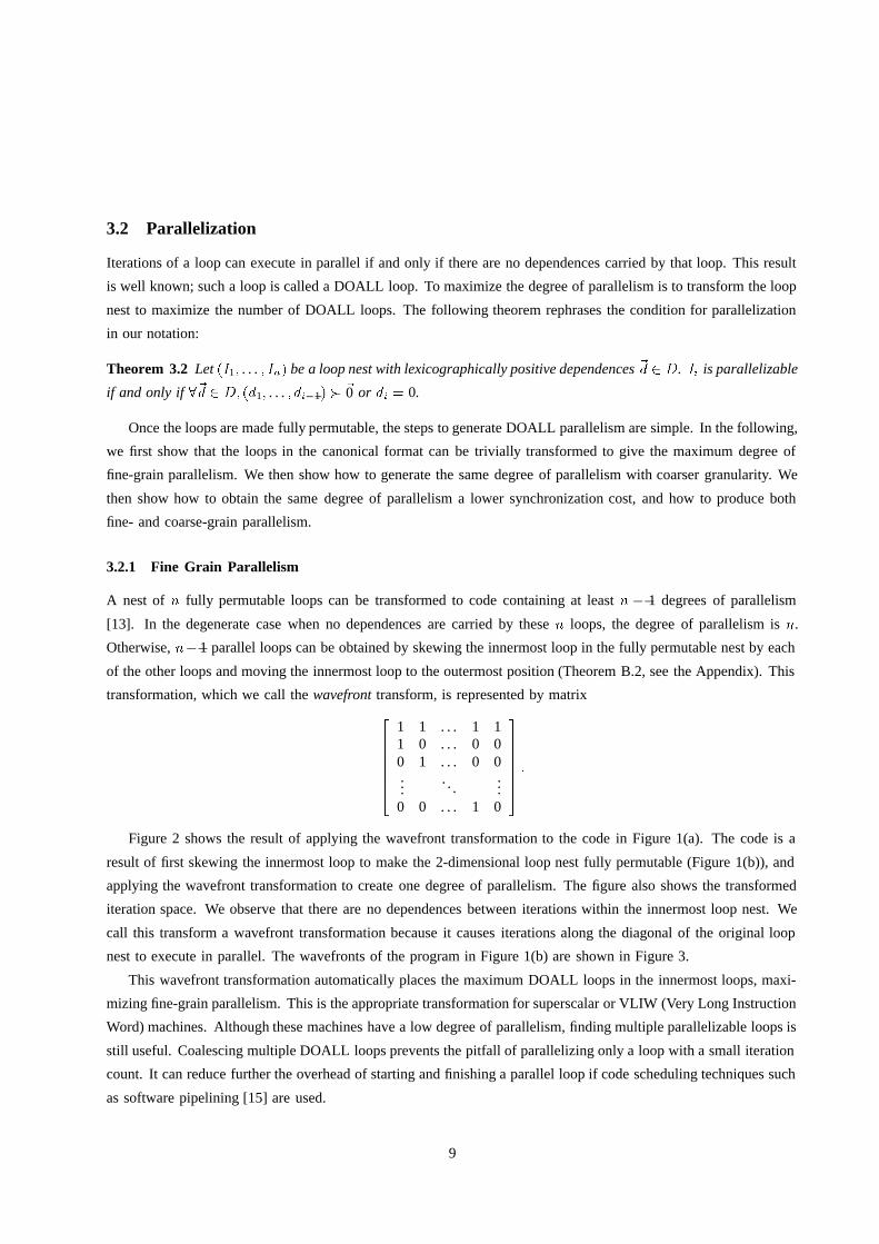
A nest of n fully permutable loops can be transformed to code containing at leastn � 1 degrees of parallelism
[13]. In the degenerate case when no dependences are carried by thesen loops, the degree of parallelism isn.
Otherwise,n�1 parallel loops can be obtained by skewing the innermost loop in the fully permutable nest by each
of the other loops and moving the innermost loop to the outermost position (Theorem B.2, see the Appendix). This
transformation, which we call thewavefronttransform, is represented by matrix
2
6
6
6
6
6
4
1 1 . . . 1 11 0 . . . 0 00 1 . . . 0 0...
......
0 0 . . . 1 0
3
7
7
7
7
7
5
:
Figure 2 shows the result of applying the wavefront transformation to the code in Figure 1(a). The code is a
result of first skewing the innermost loop to make the 2-dimensional loop nest fully permutable (Figure 1(b)), and
applying the wavefront transformation to create one degree of parallelism. The figure also shows the transformed
iteration space. We observe that there are no dependences between iterations within the innermost loop nest. We
call this transform a wavefront transformation because it causes iterations along the diagonal of the original loop
nest to execute in parallel. The wavefronts of the program in Figure 1(b) are shown in Figure 3.
This wavefront transformation automatically places the maximum DOALL loops in the innermost loops, maxi-
mizing fine-grain parallelism. This is the appropriate transformation for superscalar or VLIW (Very Long Instruction
Word) machines. Although these machines have a low degree of parallelism, finding multiple parallelizable loops is
still useful. Coalescing multiple DOALL loops prevents the pitfall of parallelizing only a loop with a small iteration
count. It can reduce further the overhead of starting and finishing a parallel loop if code scheduling techniques such
as software pipelining [15] are used.
9

for I 01 := 0 to 16 do
doall I 02 := max(0,d(I 01 � 6)=2e) to min(5,bI01=2c) do
a[I 01 � 2I 02 + 1] := 1/3 * (a[I 01 � 2I 02] + a[I01 � 2I 02 + 1]
+ a[I 01 � 2I 02 + 2]);
T =
�
1 11 0
��
1 01 1
�
=
�
2 11 0
�
D
0
= TD = f(1; 0); (2; 1); (1; 1)g
I’ 1

3.2.2 Coarsest Granularity of Parallelism
For MIMD machines, having as many outermost DOALLs as possible reduces the synchronization overhead. The
wavefront transformation produces the maximal degree of parallelism, but makes the outermost loop sequential, if
any are. For example, consider the following loop nest:
for I1 := 1 to N do
for I2 := 1 to N do
a[I1,I2] = f(a[I1 � 1,I2 � 1]);
This loop nest has the dependence(1; 1), so the outermost loop is sequential and the innermost loop a doall. The
wavefront transformation
�
1 11 0
�
does not change this. In contrast, the unimodular transformation
�
1 �10 1
�
transforms the dependence to(0; 1), making the outer loop a DOALL and the inner loop sequential. In this example,
the dimensionality of the iteration space is two, but the dimensionality of the space spanned by the dependence
vectors is only one. When the dependence vectors do not span the entire iteration space, it is possible to perform
a transformation that makes outermost DOALL loops [14].
By choosing the transformation matrixT with first row ~
t1 such that~t1 �
~
d= 0 for all dependence vectors~
d, the
transformation produces an outermost DOALL. In general, if the loop nest depth isn and the dimensionality of the
space spanned by the dependences isn
d
, it is possible to make the firstn� n
d
rows of a transformation matrixT
span theorthogonal subspaceS of the space spanned by the dependences. This will produce the maximal number
of outermost DOALL loops within the nest.
A vector~s is in S if and only if 8~d
: ~s � ~d= 0, so thatS is the nullspace (kernel) of the matrix that has the
dependences vectors as rows. Theorem B.4 shows how to construct a legal unimodular transformationT that makes
the first jSj = n � n
d
rows spanS. Thus the outerjSj loops after transformation are DOALLs. The remaining
loops can be skewed to be fully permutable, and then wavefronted to getn
d
� 1 degrees of parallelism.
A practical though non-optimal approach for making outer loops DOALL is simply to identify loopsI
i
such that
all di
are zero. Those loop can be made outermost DOALLs. The remaining loops in the tile can be wavefronted
to get the remaining parallelism.
3.2.3 Tiling to Reduce Synchronization
It is possible to reduce the synchronization cost and improve the data locality of parallelized loops via an optimization
known astiling [25, 26]. Tiling is not a unimodular transformation. In general, tiling maps ann-deep loop nest
into a 2n-deep loop nest where the innern loops include only a small fixed number of iterations. Figure 4 shows
the code after tiling the example in Figure 1(b), using a tile size of 2� 2. The two innermost loops execute the
iterations within each tile, represented as 2� 2 squares in the figure. The two outer loops, represented by the two
axes in the figure, execute the 3� 4 tiles. As the outer loops the of tiled code control the execution of the tiles, we
will refer to them as thecontrolling loops.
The same property that supports parallelization, full permutability, is also the key to tiling:
Theorem 3.3 LoopsIi
throughIj
of a legal computation can be tiled if the loopsIi
throughIj
are fully permutable.
11

for II 01 := 0 to 5 by 2 do
for II 02 := 0 to 11 by 2do
for I 01 := II
0
1 to min(5,II01 + 1) do
for I 02 := max(I 01, II0
2) to min(6+I01, II 02+1) do
a[I 02 � I
0
1 + 1] := 1/3 * (a[I 02 � I
0
1] + a[I02 � I
0
1 + 1]
+ a[I 02 � I
0
1 + 2]);
n
[25]. After tiling, instead of skewing the loops statically to form DOALL loops, the computation is allowed to skew
dynamically by explicit synchronization between data dependent tiles. In the DOALL loop approach, tiles of each
level must be completed before the processors may go on to the next, requiring a global barrier synchronization.
In the DOACROSS model, each tile can potentially execute as soon as it is legal to do so. This ordering can be
enforced by local synchronization. Furthermore, different parts of the wavefront may proceed at different rates as
determined dynamically by the execution times of the different tiles. In contrast, the machine must wait for the
slowest processor at every level with the DOALL method.
Tiling has two other advantages. First, within each tile, fine-grain parallelism can easily be obtained by skewing
the loopswithin the tile and moving the DOALL loop innermost. In this way, we can obtain both coarse- and
fine-grain parallelism. Second, tiling can improve data locality if there is data reuse across several loops [10, 24].
3.3 Summary
Using the loop transformation theory, we have shown a simple algorithm in exploiting both coarse- and fine-grain
parallelism for loops with distance vectors. The algorithm consists of two steps: the first is to transform the code
into the canonical form of a fully permutable loop nest. The second tailors the code to specific architectures via
wavefront and tiling transformations.
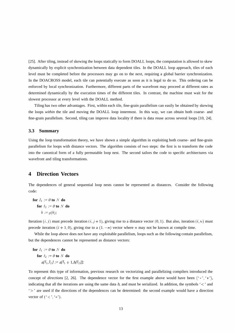
4 Direction Vectors
The dependences of general sequential loop nests cannot be represented as distances. Consider the following
code:
for I1 := 0 to N do
for I2 := 0 to N do
b := g(b);
Iteration(i; j) must precede iteration(i; j+1), giving rise to a distance vector(0; 1). But also, iteration(i; n) must
precede iteration(i + 1; 0), giving rise to a(1;�n) vector wheren may not be known at compile time.
While the loop above does not have any exploitable parallelism, loops such as the following contain parallelism,
but the dependences cannot be represented as distance vectors:
for I1 := 0 to N do
for I2 := 0 to N do
a[I1,I2] := a[I1 + 1,b[I2]];
To represent this type of information, previous research on vectorizing and parallelizing compilers introduced the
concept ofdirections [2, 26]. The dependence vector for the first example above would have been(‘ � ’ ; ‘ � ’),
indicating that all the iterations are using the same datab, and must be serialized. In addition, the symbols ‘< ’ and
‘ > ’ are used if the directions of the dependences can be determined: the second example would have a direction
vector of(‘ < ’ ; ‘ �’).
13
We would like to extend the mathematical framework used on distance vectors to include directions. To do so,
we make one key modification to the existing convention: legal “direction vectors” must also be “lexicographically
positive”. This modification makes it possible to use the same simple legality test for compound transformations
involving direction vectors.
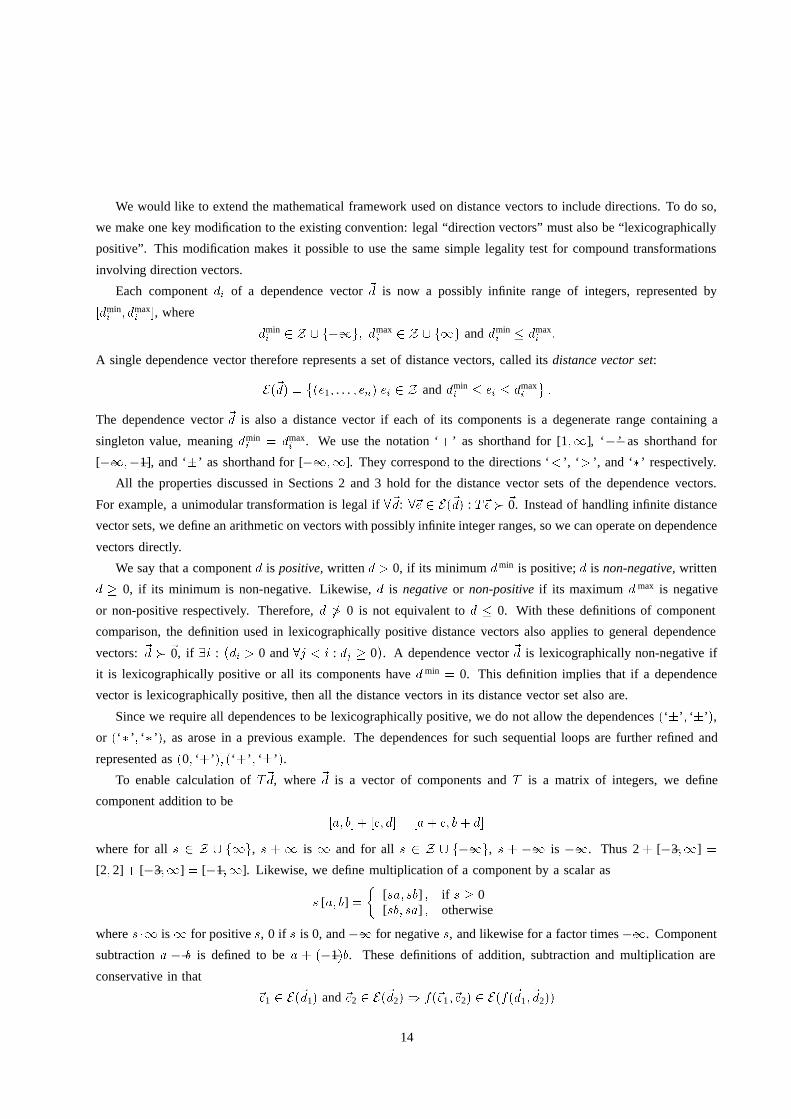
Each componentdi
of a dependence vector~d
is now a possibly infinite range of integers, represented by
[d
mini
; d
maxi
], where
d
mini
2 Z [ f�1g; d
maxi
2 Z [ f1g anddmini
� d
maxi
:
A single dependence vector therefore represents a set of distance vectors, called itsdistance vector set:
E(
~
d) =
�
(e1; . . . ; en
)je
i
2 Z anddmini
� e
i
� d
maxi
:
The dependence vector~d
is also a distance vector if each of its components is a degenerate range containing a
singleton value, meaningdmini
= d
maxi
. We use the notation ‘+ ’ as shorthand for [1;1], ‘ � ’ as shorthand for
[�1;�1], and ‘�’ as shorthand for [�1;1]. They correspond to the directions ‘< ’, ‘ > ’, and ‘�’ respectively.
All the properties discussed in Sections 2 and 3 hold for the distance vector sets of the dependence vectors.
For example, a unimodular transformation is legal if8
~
d: 8~e 2 E(~
d) : T~e � ~0. Instead of handling infinite distance
vector sets, we define an arithmetic on vectors with possibly infinite integer ranges, so we can operate on dependence
vectors directly.
We say that a componentd is positive, writtend > 0, if its minimumd
min is positive;d is non-negative, written
d � 0, if its minimum is non-negative. Likewise,d is negativeor non-positiveif its maximum d
max is negative
or non-positive respectively. Therefore,d 6> 0 is not equivalent tod � 0. With these definitions of component
comparison, the definition used in lexicographically positive distance vectors also applies to general dependence
vectors:~d�
~0, if 9i :�
d
i
> 0 and8j < i : dj
� 0�
. A dependence vector~d
is lexicographically non-negative if
it is lexicographically positive or all its components havedmin= 0. This definition implies that if a dependence
vector is lexicographically positive, then all the distance vectors in its distance vector set also are.
Since we require all dependences to be lexicographically positive, we do not allow the dependences(‘�’ ; ‘�’),
or (‘ � ’ ; ‘ � ’), as arose in a previous example. The dependences for such sequential loops are further refined and
represented as(0; ‘+’); (‘+’ ; ‘�’ ).
To enable calculation ofT~d, where~
dis a vector of components andT is a matrix of integers, we define
component addition to be
[a; b] + [c; d] = [a+ c; b+ d]
where for alls 2 Z [ f1g, s +1 is 1 and for all s 2 Z [ f�1g, s + �1 is �1. Thus 2+ [�3;1] =
[2; 2] + [�3;1] = [�1;1]. Likewise, we define multiplication of a component by a scalar as
s [a; b] =
�
[sa; sb] ; if s � 0[sb; sa] ; otherwise
wheres �1 is 1 for positives, 0 if s is 0, and�1 for negatives, and likewise for a factor times�1. Component
subtractiona � b is defined to bea + (�1)b. These definitions of addition, subtraction and multiplication are
conservative in that
~e1 2 E(~d1) and~e2 2 E(~d2) ) f(~e1;~e2) 2 E(f(~d1;~
d2))
14

wheref is a function that performs a combination of the defined operations on its operands. The converse
~e 2 E(f(
~
d1;~
d2)))
�
9~e1 2 E(~d1) and9~e2 2 E(~d2) : f(~e1;~e2) = ~e
�
is not necessarily true.
For an example, with transformationT =
�
1 10 1
�
and ~d
= (0; ‘ + ’), the precise distance vector set of
T
~
dis f(1; 1); (2; 2); (3;3); . . .g. Using the component arithmetic defined above, the resulting dependence vector
is (‘ + ’ ; ‘ + ’), which represents the ranges of each component correctly and is the best representation of the
infinite set given the dependence representation. The choice of the direction representation is a compromise; it is
powerful enough to represent most common cases without the cost associated with the more complex and precise
representation; but the application of certain transformations may result in loss of information. This drawback of
direction vectors can be overcome by representing them as distance vectors whenever possible, since no information
is lost during distance vector manipulation. In the above example, we can represent the dependence by(0; 1) rather
than by(0; ‘+’), since by transitivity both are identical. The transformed dependence is then(1; 1), which exactly
summarizes the dependence after transformation, rather than(‘+’ ; ‘+’ ), which is imprecise.
When direction vectors are necessary, information about the dependences may be lost whenever skewing is
applied. We can only guarantee thatE�
T
�1(T
~
d)
�
� E
�
~
d
�
, but T�1(T
~
d) =
~
dis not necessarily true. Thus for
general dependence vectors, the analogue of Theorem 2.1 is a pair of more restrictive theorems.
Theorem 4.1 LetD be the set of dependence vectors of a computation. A unimodular transformationT is legal if
8
~
d2 D : T~
d�
~0.
Theorem 4.2 Let D be the set of dependence vectors of a computation. A unimodular transformationT that is a
product of only permutation and reversal matrices is legal if and only if8
~
d2 D : T~
d�
~0.
5 Parallelization with Distances and Directions
Recall that ann-deep loop nest has at leastn� 1 degrees of parallelism if its dependences are all distance vectors.
In the presence of direction vectors, not all loops can be made fully permutable, and such degrees of parallelism
may not be available. The parallelization problem therefore is to find the maximum number of parallelizable loops.
The parallelization algorithm again consists of two steps: the first to transform the loops into the canonical
form, and the second tailors it to fine- and/or coarse-grain parallelism. Instead of a single fully permutable loop
nest, the canonical format for loops with general dependences is anestof fully permutable loop nests with each
outer fully permutable loop nest made as large as possible. As we will show below, once the loops are placed in
this canonical format, we can maximize the total degree of parallelism by maximizing the degree of parallelism for
each fully permutable loop nest.
5.1 An Example with Direction Vectors
Let us first illustrate the procedure with an example.
15

for I1 := 1 to N do
for I2 := 1 to N do
for I3 := 1 to N do
(a[I1; I3],b[I1; I2; I3]) := f(a[I1; I3], a[I1 + 1; I3 � 1], b[I1; I2; I3], b[I1; I2; I3 � 1]);
The loop body above is represented by ann� n� n iteration space. The referencesa[I1; I3] anda[I1 + 1; I3 � 1]
give rise to a dependence of(1; ‘�’ ;�1). The referencesa[I1; I3] anda[I1; I3] do not give rise to a dependence of
(0; ‘�’ ; 0), which is not lexicographically positive, but rather to a dependence of(0; ‘+’ ; 0) and an anti-dependence
of (0; ‘+’ ; 0). b[I1; I2; I3] andb[I1; I2; I3] give rise to a dependence of(0; 0; 0), which we ignore since it is not a
cross-iteration edge. Finally,b[I1; I2; I3] andb[I1; I2; I3�1] give rise to a dependence of(0; 0; 1). The dependence
vectors for this nest are
D = f(0; ‘+’ ; 0); (1; ‘�’ ;�1); (0; 0; 1)g :
None of the three loops in the source program can be parallelized as it stands; however, there is one degree of
parallelism that can be exploited at either a coarse or fine grain level.
By permuting loopsI2 andI3 loops, and skewing the new middle loop with respect to the outer by a factor of
1, the algorithm described in Section 6 transforms the code to canonical form:
for I
0
1 := 1 to N do
for I
0
2 := I
0
1 + 1 to I
0
1 +N do
for I
0
3 := 1 to N do
(a[I01; I0
2 � I
0
1],b[I 01; I0
3; I0
2 � I
0
1]) :=
f(a[I 01; I0
2 � I
0
1], a[I01 + 1; I 02 � I
0
1 � 1], b[I 01; I0
3; I0
2 � I
0
1], b[I 01; I0
3; I0
2 � I
0
1 � 1]);
The transformation matrixT and the transformed dependencesD
0 are
T =
2
4
1 0 01 1 00 0 1
3
5
2
4
1 0 00 0 10 1 0
3
5
=
2
4
1 0 01 0 10 1 0
3
5
and
D
0
= f(0; 0; ‘+’); (1; 0; ‘�’ ); (0; 1; 0)g:
The transformation is legal since the resulting dependences are all lexicographically positive. The resulting two
outermost loops form one set of fully permutable loops, since interchanging these loops leaves the dependences
lexicographically positive. The last loop is in a permutable loop nest by itself.
The two-loop fully permutable set can be transformed to provide one level of parallelism by application of the
wavefront skew. The transformation matrixT 0 for this phase of transformation, and the transformed dependences
D
00 are
T
0
=
2
4
1 1 01 0 00 0 1
3
5
and
D
00
= f(0; 0; ‘+’ ); (1; 1; ‘�’); (1; 0; 0)g
16

and the transformed code is
for I
00
1 := 3 to 3N do
doall I 002 := max(1,d(I001 �N )/2e) to min(N ,b(I001 � 1)/2c) do
for I
00
3 := 1 to N do
(a[I002 ; I00
1 � 2I002 ],b[I 002 ; I00
3 ; I00
1 � 2I002 ]) :=
f(a[I 002 ; I00
1 � 2I002 ], a[I002 + 1; I 001 � 2I002 � 1], b[I 002 ; I00
3 ; I00
1 � 2I002 ], b[I 002 ; I00
3 ; I00
1 � 2I002 � 1]);
Applying this wavefront transformation to all the fully permutable loop nests will produce a loop nest with the
maximum degree of parallelism. For some machines, tiling may be preferable to wavefronting, as discussed in
Section 3.2.3.
To implement this technique, there is no need to generate code for the intermediate step. The transformation to
get directly from the example to the final code is simply
T
00
= T
0
T =
2
4
1 1 01 0 00 0 1
3
5
2
4
1 0 01 0 10 1 0
3
5
=
2
4
2 0 11 0 00 1 0
3
5
5.2 Canonical Form: Fully Permutable Nests
The parallelization algorithm attempts to create the largest possible fully permutable loop nests, starting from the
outermost loops. It first applies unimodular transformations to move loops into the outermost fully permutable
loop nest, if dependences allow. Once no more loops can be placed in the outermost fully permutable loop nest,
it recursively places the remaining loops into fully permutable nests further in. The code for this algorithm, called
Make Nests, is presented in Appendix A. It callsFind FP Nest to choose the fully permutable nest to place
outermost at each step in the algorithm; that algorithm is discussed in Section 6.
For loops whose dependences are distance vectors, Section 3 shows that their parallelism is easily accessible
once they are made into a fully permutable nest. Similarly, once a loop nest with general dependence vectors is
put into a nest of largest fully permutable nests, its parallelism is readily extracted. This canonical form has three
important properties that simplify its computation and make its parallelism easily exploitable:
1. The largest, outermost fully permutable nest is unique in the loops it contains, and is a superset of all possible
outermost permutable loop nests (Theorem B.5).
2. If a legal transformation exists for a loop nest originally, then there exists alegal transformation such that after
application the nest has the largest outermost fully permutable nest possible (Theorem B.3). This property
makes it safe to use a greedy algorithm that constructs fully permutable loop nests incrementally starting with
the outermost fully permutable loop nest and working inwards.
3. Finally, a greedy algorithm that places the largest outermost fully permutable loop nest, and then recursively
calls itself on the remaining loops to place loops further in, exposes the maximum degree of parallelism
possible via unimodular transformation (Theorem B.6). The maximum degree of parallelism in a loop nest
is simply the sum of the maximal degree of parallelism of all the fully permutable nests in canonical form.
17

5.3 Fine and Coarse Grain Parallelism
To obtain the maximum finest granularity of parallelism, we perform a wavefront skew on each fully permutable
nests, and permute them so that all the DOALL loops are innermost, which is always legal.
To obtain the coarsest granularity of parallelism, we simply transform each fully permutable nest to give the
coarsest granularity of parallelism, as discussed in Section 3.2.2. If the fully permutable nest contains direction
vectors, the technique of Section 3.2.2 must be modified slightly.
Let S be the orthogonal subspace of the dependences, as in Section 3.2.2. Although the dependences are
possibly directions, we can still calculate this space precisely. Since the nest is fully permutable,d
mink
� 0. We can
assume without loss of generality thatdmaxk
= d
mink
or dmaxk
= 1 by enumerating all finite ranges of components.
If some component of~d
is unbounded, that isdmaxk
= 1, then our requirement on~s 2 S that~s � ~d= 0, implies
that sk
= 0. This puts the same constraint onS as if there had been a distance vector(0; . . . ; 0; 1; 0; . . .; 0), with a
single 1 in thek-th entry. Thus, we can calculateS by finding the nullspace of the matrix with rows consisting of
(d
min1 ; . . . ; dmin
n
) and of the appropriate(0; . . . ; 0; 1;0; . . .; 0) vectors.
These rows are a superset of the dependences within the fully permutable loop nest, but they are all lexico-
graphically positive and all their elements are non-negative. Thus, we can use these as the distance vectors of the
nest and apply the technique of Section 3.2.2 for choosing a legal transformationT to apply to make the firstjSj
rows of the transformation matrix spanS, and the technique will succeed. SinceS is calculated precisely and the
first jSj rows ofT spanS, the result is optimal.
6 Finding Fully Permutable Loop Nests
In this section, we discuss the algorithm for finding the largest outermost fully permutable loop nest; this is the
key step in parallelization of a general loop nest. Finding the largest fully permutable loop nest in the general
case is expensive. A related but simpler problem, referred to here as the time cone problem, is to find a linear
transformation matrix for afinite set of distance vectors such that the first components of all transformed distance
vectors are all positive [12, 13, 18, 21]. This means that the rest of the loops are DOALL loops. We have shown that
if all the distance vectors are lexicographically positive, this can be achieved by first skewing to make the loops fully
permutable, and wavefronting to generate the DOALL loops. However, if the distances are not lexicographically
positive, the complexity of typical methods to find such a transformation assuming one exists is at leastO(d
n�1),
whered is the number of dependences andn is the loop nest depth [21]. The problem of finding the largest fully
permutable loop nest is even harder, since we need to find the largest nest for which such a transformation exists.
Our approach is to use a cheaper technique on as many loops as possible, and apply the expensive time cone
technique only to the few remaining loops. We classify loops into three categories:
1. serializing loops, loops with dependence components including both+1 and�1; these loop cannot be
included in the outermost fully permutable nest and can be ignored for that nest.
2. loops that can be included via the SRP transformation, an efficient transformation that combines permutation,
reversal and skewing.
18

3. the remaining loops; they may possibly be included via a general transformation using the time cone method.
Appendix A contains the implementation ofFind FP Nest, the algorithm that finds an outermost fully permutable
loop nest. The parameters toFind FP Nestare the unplaced loops and the set of dependencesD not satisfied by a
loop enclosing the current loops. The routine returns the loops that were not placed in the nest, the transformation
applied, the transformed dependences, and the loops in this nest. The algorithm first removes the loops in category
1 from consideration, as discussed below, and then callsSRP to handle loops of category 2. If necessary, it then
calls GeneralTransformto handle loops of category 3.
As we expect the loop depth to be low to begin with and further reduced since most loops will typically fall
in categories 1 and 2, we recommend only a two-dimensional time cone method for loops of category 3. If there
are two or fewer loops in category 3, the algorithm is optimal, maximizing the degree of parallelism. Otherwise,
the two-dimensional time cone method can be used heuristically to find a good transformation. The algorithm can
transform the code optimally in the common cases. For the algorithm to fail to maximize the degree of parallelism,
the loop has to be at least five deep. The overall complexity of the algorithm isO(n
3d).
6.1 Serializing Loops
As proven below, a loop with both positive and negative infinite components cannot be included in the outermost
fully permutable nest. Consequently, the loop must go in a fully permutable nest further in, and cannot be run in
parallel with other loops in the outermost fully permutable nest. We call such a loop aserializingloop.
Theorem 6.1 If loop I
k
has dependences such that9~d2 D : dmin
k
= �1 and 9~d2 D : dmax
k
= 1 then the
outermost fully permutable nest consists only of a combination of loops not includingI
k
.
Proof: 9
~
d2 D : dmin
k
= �1 implies that the transformationT that producesm outermost fully permutable loop
nests must be such that8i � m : ti;k
� 0. Likewise,9~d2 D : dmax
k
= 1 implies that8i � m : ti;k
� 0. Thus if
9
~
d2 D : (dmin
k
= �1) ^ 9
~
d2 D : (dmax
k
= 1) then it must be the case that8i � m : ti;k
= 0. Thus, none of the
m outermost loops after transformation contains a component ofI
k
. 2
In our example in Section 5, the middle loop is serializing, so cannot be in the outermost fully permutable
loop nest. Once the other two loops are placed outermost, the only dependence fromD
0 that is not already made
lexicographically positive by the first two loops is(0; 0; ‘+’), so that for the next fully permutable nest, there were
no more serializing loops that had to be removed from consideration.
When a loop is removed from consideration, the resulting dependences are no longer necessarily lexicographi-
cally positive. For example, suppose a loop nest has dependences
f(1; ‘�’ ; 0; 0); (0; 1;2;�1); (0;1;�1; 1)g:
The second loop is serializing, so we only need to consider placing in the outermost nest the first, third and fourth
loops. If we just examine the dependences for those loopsf(1; 0; 0); (0; 2;�1); (0;�1; 1)g, we see that some
dependences become lexicographically negative.
19

6.2 The SRP Transformation
Now that we have eliminated serializing loops from consideration for the outermost fully permutable nest, we apply
the SRP transformation. SRP is an extension of the skewing transformation we used in Section 3 to make a nest
with lexicographically positive distances fully permutable. This technique is simple and effective in practice. The
loop in Section 5 is an example of code that is amenable to this technique.
We first consider the effectiveness of skewing when applied to loops with general dependence vectors. First,
there may not be a legal transformation that can make two loops with general dependences fully permutable. For
example, no skewing factor that can make the components of vector(1; ‘� ’) all nonnegative. Moreover, the set
of dependences vectors under consideration may not even be lexicographically positive, as discussed above. Thus,
even if the dependences are all distance vectors, it is not necessarily the case thatn � 1 parallel loops can be
extracted. For example, suppose a subset of two loops in a loop nest has dependence vectorsf(1;�1); (�1; 1)g.
These dependences are anti-parallel, so no row of any matrixT can have a non-negative dot product with both
vectors, unless the row itself is the zero vector, which would make the matrix singular. Nonetheless, there are many
common cases for which a simple reverse and skew transformation can extract parallelism from the code.
Theorem 6.2 Let L = fI1; . . . ; In
g be a loop nest with lexicographically positive dependences~
d2 D, and
D
i
= f
~
d2 Dj(d1; . . . ; d
i�1) 6� ~0g. Loop Ij
can be made into a fully permutable nest with loopI
i
, wherei < j,
via reversal and/or skewing, if
8
~
d2 D
i : (dminj
6= �1^ (d
minj
< 0 ! d
mini
> 0)) or
8
~
d2 D
i : (dmaxj
6= 1^ (d
maxj
> 0! d
mini
> 0)):
Proof: All dependence vectors for which(d1; . . . ; di�1) � ~0 do not prevent loopsI
i
and Ij
from being fully
permutable and can be ignored. If
8
~
d2 D
i : (dminj
6= �1^ (d
minj
< 0! d
mini
> 0))
then we can skew loopIj
by a factor off with respect to loopIi
where
f � maxf
~
dj
~
d2D
i
^d
mini
6=0gd�d
minj
=d
mini
e
to make loopIj
fully permutable with loopIi
. If instead the condition
8
~
d2 D
i : (dmaxj
6= 1^ (d
maxj
> 0! d
mini
> 0)):
holds, then we can reverse loopIj
and proceed as above.2
From this theorem, we derive theFind Skew algorithm in the appendix. It takes as inputD, the set of
dependences that have not been satisfied by loops outside this loop nest. It also takes as input the loopI
j
that is to
be added, if possible, into the current fully permutable nest, which is also input. It attempts to skew loopI
j
with
respect to the fully permutable loop nest so that all dependences (that are not satisfied by outer loops) will have
non-negativedj
components. It returns whether it was able to successfully skew, as well as the skews performed
20

and the new dependence vectors and the transformation applied. The run time for this algorithm isO(jN jd+ d),
whered is the number of dependences in the loop nest. IfN is empty, then this routine returns successfully if loop
I
j
was such that alldj
� 0, or if loop Ij
could be reversed to make that so.
The SRP transformation builds a fully permutable nest. The algorithm begins with no loops in the nest and
successively callsFind Skew, permuting loops into the nest thatFind Skew successfully made fully permutable
with the other loops in the nest. The SRP algorithm fails whenFind Skewcannot place any remaining loop into
the nest. The code forSRPis shown in the appendix. It takes as input the set of dependencesD that have not been
satisfied by the loops outside this nest, the fully permutable nest so far (so that it can be used in conjunction with
other algorithms that also build fully permutable nests) and the set of loopsI that are unplaced and not serializing.
It returns the transformation performedT , the new dependencesD, and the loops that SRP failed to place.
The SRP transformation has several important properties, proofs of which can be found in [23]. First, although
the entire transformation is constructed as a series of a permutation, reversal and skew combination, the complete
transformation can be expressed as the application of one permutation transformation, followed by a reversal of
zero or more of the loops, followed by a skew. That is, we can write the transformationT asT = SRP , whereP
is a permutation matrix,R is a diagonal matrix with each diagonal entry being either 1 or�1 (loop reversal), and
S is a lower triangular matrix with ones on the diagonal (loop skewing). Note that whileT produces a legal fully
permutable loop nest, just applyingP may not produce a legal loop nest.
Second, as an extension to the skewing transform presented in Section 3, SRP converts a loop nest with
only lexicographically positive distance vectors into a single fully permutable loop nest. Thus SRP finds the
maximum degree of parallelism for loops in this special case. Generalizing this observation, if there exists an SRP
transformation that makes dependence vectors lexicographically positive, and none of the transformed dependence
vectors has an unboundedly negative component (8
~
d: dmin
6= �1), our algorithm again will place all the loops
into a single fully permutable loop nest.
Third, the Find FP Nest algorithm that uses SRP to find successive fully permutable loop nests will always
produce a legal order for the loops if all the dependences were initially lexicographically positive, or could have
been made so by some SRP transformation.
Fourth, the complexity of the SRP transformation algorithm isO(m
2d) wherem is the number of loops
considered. IfFind FP Nestdoes not attempt transformations on loops in category 3, then it isO(n
2d) wheren is
the number of loops in the entire loop nest.
Fifth, if Find FP Nestwith SRP fails to create any fully permutable nest with more than one loop, then there
is no unimodular transformation that could have done so. To rephrase slightly,Find FP Nestwith SRP produces
DOALL parallelism whenever any is available via a unimodular transformation, even if it finds less than the optimal
degree of parallelism.
6.3 General Two-Dimensional Transformations
In general, the SRP transformation alone cannot find all possible parallelism. Consider again the example of a loop
with dependencesD = f(1; ‘�’ ; 0; 0); (0;1; 2;�1); (0; 1;�1;1)g. The first loop can obviously be placed in the out-
21

f( ; ; ); ( ; ;� ); ( ;� ; )g
T T ( ;� ) T (� ; )
T
O(d)
~
t8
~
d2 D
~
t�
~
d> T
~
t
~
t
~
t
~
t
( ;� ) (� ; )
~
t
~
t
~
t
~
t
(t ; t ) = ( ; )
T
T =
�
t t
x y
�
:
x y T
t y � t x = t t x y

Extended Euclidean algorithm. For our example, Euclid’s algorithm producesx = 1 andy = 2, and we get
T =
�
2 31 2
�
andT�1=
�
2 �3�1 2
�
:
The (I1; I2) iteration is transformed byT into the (I
0
1; I0
2) iteration. By the construction of the transformationT ,
the I 01 component of all dependences are positive, so all dependences are lexicographically positive. Thus we can
skew theI02 loop with respect to theI 01 loop by calling SRP to make the nest fully permutable.
By incorporating the two-dimensional transform intoFind FP Nests, the execution time of the complete paral-
lelizing algorithm becomes potentiallyO(n
3d). In the worst case, SRP takesO(n
2d) but places no loops in the
nest, and thenFind FP Nestsearches
�
n
2
�
pairs of loops to find a pair for which the two dimensional time cone
method succeeds. Thus at worst it takesO(n
2d) to place two loops into the nest, which makes the worst case run
time of the algorithmO(n
3d). In the case that SRP was sufficient to find the maximum degree of parallelism, the
two-dimensional transformation portion of the algorithm is never executed, and the run time of the parallelization
algorithm remainsO(n
2d).
7 Implementating the Transformation
In this section, we discuss how to express a loop transformed by unimodular transformation and tiling back as
executable code. In either case, the problem consists of two parts: rewriting the body of the loop nest and rewriting
the loop bounds. It is easy to rewrite the body of the loop nest; the difficult part is the loop bounds. We first
discuss unimodular transformations, then tiling.
7.1 Unimodular Transformations
Suppose we have the loop nest
for I1 := . . .
. . .
for I
n
:= . . .
S(I1,. . .,In
);
to which we apply the unimodular transformationT . The transformation of the bodyS only requires that for
j = 1; . . . ; n, Ij
be replaced by the appropriate linear combination ofI
0s, where theI0s are the indices for the
transformed loop nest; that is:2
6
4
I1...
I
n
3
7
5
= T
�1
2
6
4
I
0
1...
I
0
n
3
7
5
:
Performing this substitution is all that is required for the loop body. The remainder of this section discusses the
transformation on the loop bounds.
23

7.1.1 Scope of Allowable Loop Bounds
Our method of determining the loop bounds after unimodular transformation requires that the loop bounds be of
the form
for I
i
:= max(L1i
; L
2i
; . . .) to min(U1i
; U
2i
; . . .) by 1 do
where
L
j
i
=
l�
l
j
i;0 + l
j
i;1I1 + . . .+ l
j
i;i�1Ii�1
�
=l
j
i;i
m
andU j
i
=
j�
u
j
i;0 + u
j
i;1I1 + . . .+ u
j
i;i�1Ii�1
�
=u
j
i;i
k
and alllji;k
anduji;k
are known constants, except possibly forl
j
i;0 anduji;0, which must still be invariant in the loop
nest. (If a ceiling occurs where we need a floor it is a simple matter to adjustl
j
i;0 anduji;0 and replace the ceiling
with the floor, and likewise if a floor occurs where we need a ceiling.) If any loop increments is not one, then it
must first be made so via loop normalization [1]. If the bounds are not of the proper form, then the given loop
cannot be involved in any transformations, and the loop nest is effectively divided into two: those outside the loop
and those nested in the loop.
It is important to be able to handle loop bounds of this complexity. Although programmers do not often write
bound expressions with minima, maxima and integer divisions, loop transformations can create them. In particular,
we consider tiling as separate from unimodular transformation, so in the case of double level blocking, we can
transform the nest with a unimodular matrix, tile, and then further transform the tiled loops and tile again inside.
Since tiling can create loops of this complexity, we wish to be able to handle them.
7.1.2 Transforming the Loop Bounds
We outline our method for determining the bounds of a loop nest after transformation by unimodular matrixT .
We explain the general method and demonstrate it by permuting the loop nest in Figure 7 to makeI 3 the outermost
loop andI1 the innermost loop, i.e. by applying the transformation
2
4
0 0 10 1 01 0 0
3
5
:
Step 1: Extract inequalities. The first step is to extract all inequalities from the loop nest. Using the notation
from Section 7.1.1, the bounds can be expressed as a series of inequalities of the formI
i
� L
j
i
andIi
� U
j
i
.
Step 2: Find the absolute maximum and minimum for each loop index. The second step is to use the
inequalities to find the maximum and minimum possible values of each loop index. This can be easily done from
the outermost to the innermost loop by substituting the maxima and minima outside the current loop of interest into
the bound expressions for that loop. That is, since the lower bound ofI
i
is maxj
(L
j
i
), the smallest possible value
for Ii
is the maximum of the smallest possible values ofL
j
i
.
We useImini
andLj;mini
to denote the smallest possible value forI
i
andLji
respectively, and we useImini;j
k
to
denote eitherImink
or Imaxk
, whichever minimizes(lji;k
I
mini;j
k
)=l
j
i;i
:
I
mini
= maxj
(L
j;mini
)
24

An example loop nest:
for I1 := 1 to n1 do
for I2 := 2I1 to n2 do
for I3 := 2I1 + I2 � 1 to min(I2; n3) do
S(I1; I2; I3);
Step 1: Extract inequalities:I1 � 1 I1 � n1
I2 � 2I1 I2 � n2
I3 � 2I1 + I2 � 1 I3 � I2 I3 � n3
Step 2: Find absolute maximum and minimum for each loop index:
I
min1 = 1 I
max1 = n1
I
min2 = 2� 1 = 2 I
max2 = n2
I
min3 = 2� 1+ 2� 1 = 3 I
max3 = min(n2; n3)
Step 3: Transform indices:I1 ) I
0
3 I2 ) I
0
2 I3 ) I
0
1
Inequalities Maxima and minimaI
0
3 � 1 I
0
3 � n1 I
0min1 = 3 I
0max1 = min(n2; n3)
I
0
2 � 2I03 I
0
2 � n2 I
0min2 = 2 I
0max2 = n2
I
0
1 � 2I03 + I
0
2 � 1 I
0
1 � I
0
2 I
0
1 � n3 I
0min3 = 1 I
0max3 = n1
Step 4: Calculate new loop bounds:
Index Inequality (index on LHS) Substituting inI 0min andI0max ResultI
0
2 I
0
2 � 2I03 I
0
2 � 2 I
0
2 � 2I
0
2 � I
0
1 I
0
2 � I
0
1I
0
2 � n2 I
0
2 � n2
I
0
2 � I
0
1 � 2I03 + 1 I
0
2 � I
0
1 � 1 I
0
2 � I
0
1 � 1
I
0
3 I
0
3 � 1 I
0
3 � 1I
0
3 � n1 I
0
3 � n1
I
0
3 � (I
0
1 � I
0
2 + 1)=2 I
0
3 � b(I
0
1 � I
0
2 � 1)=2c
The loop nest after transformation:
for I
0
1 := 3 to min(n3; n2) do
for I
0
2 := I
0
1 to min(n2; I0
1 � 1) do
for I
0
3 := 1 to min(n1; b(I0
1 � I
0
2 + 1)=2c) do
S(I 03; I0
2; I0
1);
Figure 7: Finding the loop bounds after unimodular transformation.
25

where
L
j;mini
=
&
l
j
i;0 +
i�1X
k=1
l
j
i;k
I
mini;j
k
!
=l
j
i;i
'
and
I
mini;j
k
=
�
I
mink
; sign(lji;k
) = sign(lji;i
)
I
maxk
; otherwise:
Similar formulas hold forU j;mini
, Lj;maxi
andU j;maxi
.
Step 3: Transform indices. We now use(I1; . . . ; In
) = T
�1(I
0
1; . . . ; I0n
) to replace theIj
s variables in the
inequalities byI 0j
s. The maximum and minimum for a givenI0j
is easily calculated. For example, ifI01 = I1� 2I2,
thenI 0max1 = I
max1 � 2Imin
2 andI0min1 = I
min1 � 2Imax
2 . In general, we use(I01; . . . ; I0n
) = T (I1; . . . ; In
) to express the
I
0
j
s in terms of theIj
s. If I0j
=
P
a
j
I
j
, then
I
0mink
=
n
X
k=1
a
j
�
I
minj
a
j
> 0I
maxj
otherwise
and likewise forI 0maxk
.
Step 4: Calculate new loop bounds. The lower and upper bounds for loopI 01 are justI 0min1 andI0max
1 . Otherwise,
to determine the loop bounds for loop indexI 0i
, we first rewrite each inequality from step three containingI
0
i
by
solving for I 0i
, producing a series of inequalities of the formI 0i
� f(. . .) and I0i
� f
0
(. . .). Each inequality of the
form I
0
i
� f(. . .) contributes to the upper bound. If there is more than one such expression, then the minimum of
the expressions is the upper bound. Likewise, each inequality of the formI
0
i
� f
0
(. . .) contributes to the lower
bound, and the maximum of the right hand sides is taken if there is more than one.
An inequality of the formI 0i
� f
0
(I
0
j
) contributes to the lower bound of loop indexI 0i
. If j < i, meaning that
loop I
0
j
is outside loopI 0i
, then the expression does not need to be changed since the loop bound ofI
0
i
can be a
function of the outer indexI 0j
. If loop I
0
j
is nested within loopI 0i
, then the bound for loop indexI 0i
cannot be a
function of loop indexI 0j
. In this case we must replaceI0i
by its minimum or maximum, whichever minimizesf . A
similar procedure is applied to the upper loop bounds. The loop bounds produced as a result of these manipulations
again belong to the class discussed in Section 7.1.1, so that our methods can calculate the loop bounds after further
transformation of these loops.
7.1.3 Discussion of Method
The algorithm to determining loop bounds is efficient. For ann-deep loop nest, there are at least 2n inequalities,
since each loop has at least one lower and upper bound. In general, each loop bound may be maximum and
minimum functions, with every term contributing one inequality. Let the number of inequalities beq. Both steps 1
and 2 in the algorithm are linear. The third step requires a matrix-vector multiply and a scan through the inequalities,
and so isO(n
2+ q). The fourth step is potentially the most expensive, since allq inequalities could potentially
involve all n loop indices, for a total cost ofO(nq). Thus the loop bound finding algorithm isO(nq).
26

@
@
@
@
@
@
@
@�
�
�
�
�
�
�
�
6
?
S
i
-�
S
j
6
jmin
-
imin6
jmax
-
imax
Figure 8: Tiling a trapezoidal loop (2-D)
The resulting loop nest, while correct, may contain excessive maxima and minima computation in the loop
bounds, and may contain outer loop iterations that have no loop body iterations executed. Neither of these problems
occur in the body of the innermost loop, and thus the extra computation cost should be negligible. These problems
can be removed via well known integer linear system algorithms [11].
7.2 Tiling Transformation
The technique we apply for tiling does not require any changes to the loop body. We thus discuss only the
changes to the loop nest and bounds. While it has been suggested that strip-mining and interchanging be applied to
determine the bounds of a tiled loop, this approach is not straightforward when the iteration space is not rectangular
[26]. A more direct method is as follows. When tiling, we partition the iteration space, whatever the shape of the
bounds, as in Figure 8. Each rectangle represents a computation performed by a tile; some tiles may contain little
or even no work.
Tiling a nest(Ii
; . . . ; Ij
) addsj � i + 1 controlling loops, denoted by(IIi
; . . . ; IIj
), to the loop nest. The
lower bound on theIk
is now the maximum of the original lower bound andIIk
; similarly, the upper bound is the
minimum of the original upper bound andIIk
+ S
k
� 1, whereSk
is the size of the tile in thek loop. For loop
II
k
, the lower and upper bounds are simply the absolute minimum and maximum values of the originalI
k
, and the
step size isSk
. As shown in Figure 8, some of these tiles may be empty. The time wasted in determining that the
tile is empty should be negligible when compared to the execution of the large number of non-empty tiles in the
loop. Once again, these problems can be removed via well known integer linear system algorithms [11].
Applying these methods to the permuted example loop nest from Figure 7, we can tile to get the following:
for II
0
1 := 3 to min(N2; N3) by S1 do
for II
0
2 := 2 to N2 by S2 do
for II
0
3 := 1 to N1 by S3 do
for I
0
1 := max(3; II01) to min(N3; N2; II0
1 + S1 � 1) do
for I
0
2 := max(I01; II0
2) to min(N2; I0
1 � 1; II 02 + S2 � 1) do
for I
0
3 := max(1; II03) to min(N1; b(I0
1 � I
0
2 + 1)=2c; II 03 + S3 � 1) do
S(I 03; I0
2; I0
1);
27

Note thatI 01, I02 andI03 are fully permutable, and so are theII 01, II02 andII03. Each of these two groups can further be
transformed to deliver parallelism at the fine and/or coarse granularity of parallelism, as discussed in Section 3.2.3.
The same loop bound conversion algorithm described here is sufficient to support such further transforms, because
the loop bounds of each group again satisfy the general format allowed.
8 Conclusions
This paper proposes a new approach to transformations for general loop nests with distance and direction dependence
vectors. We unify the handling of distance and direction vectors by representing direction vectors as an infinite
set of distance vectors. In this approach, dependence vectors represent precedence constraints on the iterations
of a loop. Therefore, dependences extracted from a loop nest must be lexicographically positive. This departure
from previous research on vectorizing and parallelizing compilers leads to a simple test for legality of compound
transformations: any code transformation that leaves the dependences lexicographically positive is legal.
This model unifies all combinations of loop interchange, reversal and skewing as unimodular transformations.
The use of matrices to model transformations has previously been applied only to special cases where dependences
can be summarized by distance vectors. We extended vector arithmetic to include directions in a way such that
the important and common operations on these vectors are efficient. With this model, we can easily determine
a compound transform to be legal: a transform is legal if it yields lexicographically positive dependence vectors
when multiplied to the original dependence vectors. The ability to directly relate a compound transform to the
characteristics of the final code allows us to prune the search for the optimal transform. A problem such as
maximizing parallelism is now simply one of finding the unimodular transformation matrix that maximizes an
objective function, subject to the legality constraints.
To demonstrate the usefulness of this model, this paper applies this loop transformation theory to the problem
of maximizing the degree of coarse- or fine-grain parallelism in a loop nest. There are three main results: First, the
maximum degree of parallelism can be achieved by transforming the loops into a nest of coarsest fully permutable
loop nests, and wavefronting the fully permutable nests. Second, this canonical form of coarsest fully permutable
nests can be transformed mechanically to yield maximum degrees of coarse- and/or fine-grain parallelism. Third,
while it is expensive to find the coarsest fully permutable loop nest, our efficient heuristics can find the maximum
degrees of parallelism for loops whose nesting level is less than five.
This loop transformation theory has both theoretical and practical benefits. This matrix transformation model
makes it possible to formulate various loop transformation problems as mathematical optimization problems, prove
certain transforms to be optimal in an infinite space of general loop transforms, and to devise efficient and effective
heuristics to complex problems. Besides applying the theory to maximizing parallelism, we have successfully used
this model in developing an efficient algorithm that applies unimodular and tiling transforms to improve the data
locality of loop nests[24]. The elegance of this theory helps reduce the complexity of the implementation. Once
the dependences are extracted, the derivation of the compound transform simply consists of matrix and vector
operations. After the transformation is determined, a straightforward algorithm applies the transformation to the
loop bounds and derives the final code.
28

9 Acknowledgments
We would like to thank the other members of the SUIF compiler group at Stanford University for providing a
context in which this research could be carried out. The team includes Saman Amarasinghe, Jennifer Anderson,
Robert French, John Hennessy, Amy Lim, Dror Maydan, Karen Pieper, Michael D. Smith, Steve Tjiang, and Bob
Wilson.
References
[1] R. Allen and K. Kennedy. Automatic translation of FORTRAN programs to vector form.ACM Transactions
on Programming Languages and Systems, 9(4):491–542, 1987.
[2] U. Banerjee. Data dependence in ordinary programs. Technical Report 76-837, University of Illinios at
Urbana-Champaign, Nov 1976.
[3] U. Banerjee.Dependence Analysis for Supercomputing. Kluwer Academic, 1988.
[4] U. Banerjee. A theory of loop permutations. In2nd Workshop on Languages and Compilers for Parallel
Computing, Aug 1989.
[5] U. Banerjee. Unimodular transformations of double loops. In3rd Workshop on Languages and Compilers for
Parallel Computing, Aug 1990.
[6] R. Cytron. Compile-time Scheduling and Optimization for Asynchronous Machines. PhD thesis, University of
Illinois at Urbana-Champaign, 1984.
[7] J.-M. Delosme and I. C. F. Ipsen. Efficient systolic arrays for the solution of Toeplitz Systems: an illustration
of a methodology for the construction of systolic architectures in VLSI. Technical Report 370, Yale University,
1985.
[8] J. A. B. Fortes and D. I. Moldovan. Parallelism detection and transformation techniques useful for VLSI
algorithms.Journal of Parallel and Distributed Computing, 2:277–301, 1985.
[9] K. Gallivan, W. Jalby, U. Meier, and A. Sameh. The impact of hierarchical memory systems on linear algebra
algorithm design. Technical report, University of Illinios, 1987.
[10] D. Gannon, W. Jalby, and K. Gallivan. Strategies for cache and local memory management by global program
transformation.Journal of Parallel and Distributed Computing, 5:587–616, 1988.
[11] F. Irigoin. Partitionnement Des Boucles Imbeiquees: Une Technique D’optimisation four les Programmes
Scientifiques. PhD thesis, Universite Paris-VI, June 1987.
[12] F. Irigoin and R. Triolet. Computing dependence direction vectors and dependence cones. Technical Report
E94, Centre D’Automatique et Informatique, 1988.
29

[13] F. Irigoin and R. Triolet. Supernode partitioning. InProc. 15th Annual ACM SIGACT-SIGPLAN Symposium
on Principles of Programming Languages, pages 319–329, January 1988.
[14] F. Irigoin and R. Triolet. Dependence approximation and global parallel code generation for nested loops. In
Parallel and Distributed Algorithms, 1989.
[15] M. S. Lam. Software pipelining: An effective scheduling technique for VLIW machines. InProc. ACM
SIGPLAN 88 Conference on Programming Language Design and Implementation, pages 318–328, June 1988.
[16] D. E. Maydan, J. L. Hennessy, and M. S. Lam. Efficient and exact data dependence analysis. InProc. ACM
SIGPLAN 91 Conference on Programming Language Design and Implementation, June 1991.
[17] A. Porterfield. Software Methods for Improvement of Cache Performance on Supercomputer Applications.
PhD thesis, Rice University, May 1989.
[18] P. Quinton. The systematic design of systolic arrays. Technical Report 193, Centre National de la Recherche
Scientifique, 1983.
[19] P. Quinton. Automatic synthesis of systolic arrays from uniform recurrent equations. InProc. 11th Annual
International Symposium on Computer Architecture, June 1984.
[20] H. B. Ribas. Automatic Generation of Systolic Programs From Nested Loops. PhD thesis, Carnegie Mellon
University, June 1990.
[21] R. Schreiber and J. Dongarra. Automatic blocking of nested loops. 1990.
[22] C.-W. Tseng and M. J. Wolfe. The power test for data dependence. Technical Report Rice COMP TR90-145,
Rice University, Dec 1990.
[23] M. E. Wolf. Improving Parallelism and Data Locality in Nested Loops. PhD thesis, Stanford University, 1991.
In preparation.
[24] M. E. Wolf and M. S. Lam. A data locality optimizing algorithm. InProc. ACM SIGPLAN 91 Conference on
Programming Language Design and Implementation, pages 30–44, June 1991.
[25] M. J. Wolfe. More iteration space tiling. InSupercomputing ’89, Nov 1989.
[26] M. J. Wolfe. Optimizing Supercompilers for Supercomputers. MIT Press, 1989.
30

A The Parallelization Algorithms
algorithm Make FP Nests(D: set of dependence,n: integer)
return(success:boolean,D: set of dependence,T : matrix,fp nests:list of index);
fp nests:list of index := [ ];bot: integer := 0;T : matrix := identity;while bot< n doT
f
: matrix;top: integer := bot+1;(D,T
f
,bot) := FindFP Nest(D,top,n);if top> bot then
return (false,D,T ,fp nests);end if;fp nests := fpnests+[top];T := T
f
T ;end while;return (true,D,T ,fp nests);
end algorithm;
algorithm Find FP Nest(D: set of dependence,top: index, /*first unplaced*/n: index)
return(D: set of dependence,T : matrix,bot: index); /* last placed*/
bot: index;T ,T
g
: matrix;D
top: set of dependence :=f~d2 Dj(d1; . . .; d
top�1) 6� ~0g;I: set of index := fi 2 ftop; . . . ; ngj
8
~
d2 D
top : dmini
6= �1 or8
~
d2 D
top : dmaxi
6= 1g;(D,T ,bot,I) := SRP(D,top,top�1,I);if I 6= ; then
(D,Tg
,bot,I) := GeneralTransform(D,top,bot,I);T := T
g
T ;end if;return (D,T ,bot);
end algorithm;
algorithm SRP(D: set of dependence,top: index, /* top of fp nest*/
cur: index, /* last loop in fp nest so far*/I: set of index)
returnD: set of dependence,T : matrix,bot: index,I: set of index); /* available loops*/
done:boolean:= false;T ,T
s
,Tp
: matrix := identity;while not donedo
skewed:boolean;done :=true;foreach c 2 I repeat
(skewed,D,Ts
) := Find Skew(D,c,top,cur);if skewedthen
done :=false;T
p
:= identity with rowsc andcur +1 swapped;T := T
p
T
s
T ;D := 8
~
d2 D : swap componentsd
cur+1 anddc
;I := I � fcg; /* c now placed*/if cur+1 2 I thenI := I � fcur+1g + fcg;
end if;cur := cur+1;
end if;end foreach;
end while;return (D,T ,cur,I);
end algorithm;
algorithm Find Skew(D: set of dependence,j: index, /* candidate for skewing*/top,cur: index) /*fp nesttop to cur */
return(success:boolean,D: set of dependence,T : matrix);
N : set of index :=ftop; . . . ;curg;T : matrix := zero;D
top: set of dependence :=f~d2 Dj(d1; . . . ; d
top�1) 6� ~0g;
/* pass one: determine whether skewing possible */if 8~
d2 D
top : dminj
6= �1 and(d
minj
� 0 or 9k 2 N : dmink
> 0) thenT
j;j
:= 1;else if 8~
d2 D
top : dmaxj
6=1 and(d
maxj
� 0 or 9k 2 N : dmink
> 0) thenT
j;j
:= �1;foreach~
d2 D do d
j
:= �d
j
; end foreach;else
return (false,D,T );
31

end if;
/* pass two: determine skews */foreach~
d2 D
top doif dmin
j
< 0 thenchoose anyk : k 2 N ^ d
mink
> 0;T
j;k
:= max(Tj;k
; d�d
minj
=d
mink
e);end if;
end foreach;
/* pass three: fix dependences */foreach~
d2 D do
d
j
:= d
j
+
P
k2N
T
j;k
d
k
;end foreach;
return (true,D,T );end algorithm;
algorithm GeneralTransform(D: set of dependence,top: index, /* top of current nest*/cur: index, /*1..cur already ordered*/I: set of index)
return(D: set of dependence,T : matrix,bot: index,I: set of index)
success:boolean:= false;c1,c2: index;T
tmp
,T : matrix := identity;foreach c1; c2 2 I, c1 6= c2 do
(success,D,Ttmp
) := Find 2d Trans(D,c1,c2,cur);if successthenT := T
tmp
;cur := cur+2;if I 6= ; then
(D,Ttmp
,cur,I) := SRP(D,top,cur,I);T := T
tmp
T ;if I 6= ; then
(D,Ttmp
,cur,I) := GeneralTransform(D,top,cur,I);T := T
tmp
T ;end if;
end if;return (D,T ,cur,I);
end if;end foreach;return (D,T ,cur,I);
end algorithm;
algorithm Find 2d Trans(D: set of dependence,
c1,c2: index, /* loops to transform*/cur: index, /* 1..cur already ordered*/I: set of index)
return(success:boolean, /* true if 2D transf. exists*/D: set of dependence, /*the new dependences*/T : matrix, /* the transf. found*/I: set of index) /* unplaced loops*/
/* See Section 6.3. */end algorithm;
32

B Proofs
We first state and prove a lemma about unimodular matrices that we need for the proofs in this section.
Lemma B.1 If gcd(t1;1; t1;2; . . . ; t1;n) = 1, then ann � n unimodular matrixT exists with(t1;1; t1;2; . . . ; t1;n) as
its first row.
Proof: This lemma is true forn = 2, as we saw in Section 6.3. We prove that it is true for generaln by
mathematical induction.
If t1;i = 0 for i = 2; . . . ; n, then t1;1 is 1 or�1 and a solution is the identity matrix with the first diagonal
element replaced byt1;1. So assume at least one oft1;i is non-zero ini = 2; . . . ; n. Let g = gcd(t1;2; . . . ; t1;n). We
construct the matrix
U =
2
6
6
6
6
6
4
t1;1 t1;2 . . . t1;n
0 u2;2 . . . u2;n...
......
0 u
n�1;2 . . . u
n�1;n
x t1;2s=g . . . t1;ns=g
3
7
7
7
7
7
5
where rows 2 throughn� 1 of U are chosen so that the upper rightn� 1� n� 1 submatrix has a determinant of
�g. This is possible because a unimodular matrix exists with a first row of(t1;2=g; . . . ; t1;n=g), by the induction
hypothesis. Given this construction, the lower rightn � 1� n � 1 submatrix ofU has a determinant of�s. The
determinant ofU is therefore(t1;1)(�s) � (x)(�g) which can be written as the determinant of one of the four
matrices represented by
�
t1;1 �g
x �s
�
: The top row has a gcd of unity, so thatx ands can be chosen to make the
appropriate matrix unimodular. Thus we have constructed ann� n unimodular matrix with the required first row.
2
B.1 Parallelism in a Fully Permutable Nest
Theorem B.2 Applying the wavefront transformation
2
6
6
6
6
6
4
1 1 . . . 1 11 0 . . . 0 00 1 . . . 0 0...
. . ....
0 0 . . . 1 0
3
7
7
7
7
7
5
to a fully permutable loop nest maximizes the degree of parallelism within the nest. For ann-dimensional loop
nest, the maximal degree of parallelism isn � 1 if there are any dependences carried within the loop nest, andn
otherwise.
Proof: Suppose the fully permutable loop nest is loopsI
i
throughIj
. LetDi
= f
~
d2 Dj(d1; . . . ; d
i�1) 6� ~0g. The
dependences inDi are the only ones of interest, since all others are automatically satisfied. For all dependences~
d2 D
i, the loops are fully permutable means thatd
k
� 0 for all k = i; . . . ; j. Thus, for all~e 2 E(
~
d) either
e
i
+ . . . + e
j
> 0 or all ek
= 0. In either case, the resultingi + 1st throughjth loops are DOALL loops. It is
33

also easy to verify all dependences that were lexicographically positive before are still so. Thus the transformation
produces a legal ordering of the original nest, as well as producingj � i DOALL loops. It is not possible to have
all loops be DOALLs unless there are no dependences inD
i, in which case the above transformation also produces
all DOALL loops. 2
B.2 Legality of Making Loops Outermost
Theorem B.3 Suppose there exists a unimodular transformationT such that8~d2 D : T~
d�
~0. Let the vector~u
be such thatgcd(u1; . . . ; un
) = 1 and 8~d2 D : ~u � ~
d� 0. Then there exists a unimodular transformationU with
first row ~u such that8~d2 D : U~
d�
~0.
Proof: We first prove the theorem under the assumption that all the dependence vectors~
dare distance vectors~e.
Let~t
i
be theith row ofT , and define the constantsa1; . . . ; am
so that~u = a1~t1+. . .+a
m
~
t
m
, wheream
6= 0. We
prove the theorem by constructing a sequence ofn�n unimodular matricesU1; . . . ; Um
. EachUj
we construct will
have the property thatUj
~e �
j
~0, where�j
~0 means that the firstj components are lexicographically non-negative.
U
j
is of the form
U
j
=
�
A
j
00 I
n�m
�
T
where eachAj
is anm �m unimodular matrix andIn�m
is then�m� n�m identity matrix. That is, the first
m rows ofUj
are combinations of the firstm rows of T and the lastn �m rows ofUj
are identical to the last
n�m rows ofT . We will show thatUm
meets the requirements forU in the theorem statement.
We constructA1 by choosing as its first row(a1; . . . ; am
). Such anA1 must exist by Lemma B.1. Thus the
first row of U1 is therefore~u, and~u � ~e is given to be non-negative for all~e. ThusU1 satisfies the property that
U1~e �1 ~0.
We now constructA2 such thatU2~e �2 ~0. We define the constantsci
to be such that~t1 = c1~u1;1+ . . .+c
m
~u1;m,
where~u1;k is thekth row of U1. If m > 1, thenc2 throughcm
cannot all be zero, so we can definec0i
such that
c
0
i
= c
i
= gcd(c2; . . . ; cm
). Then we define the matrixA2 by
A2 =
2
6
4
1 0 0 . . .0 c
0
2 c
0
3 . . ....
......
. . .
3
7
5
A1
where rows 3 throughm of the premultiplying matrix are chosen to make it unimodular, as is possible from
Lemma B.1. U2 again has a first row of~u. Now we show that for all~e, U2~e �2 ~0. The first component
of U2~e is ~u � ~e, which is given to be non-negative. If it is positive, then the first two components ofU 2~e are
trivially lexicographically positive; if it is zero, we much check for the non-negativity of the second component
of U2~e. The second row ofU2 is a linear combination of~u and~t1 only. In fact, the second row ofU2 is exactly
(
~
t1 � c1~u)= gcd(c2; . . . ; cm
). When the first component ofU2~e is zero, then~u �~e is zero and the second component
of U2~e is a positive multiple of~t1 �~e. But~
t1 �~e is non-negative becauseT is a legal transformation. Thus the first
two entries ofU2~e must form a lexicographically non-negative vector.
We repeat this process, premultiplyingAj�1 to construct a new matrixA
j
with the property that for all~e,
U
j
~e �
j
~0. We achieve this by making thejth row of Uj
be a linear combination of~t
j�1 and the firstj � 1 rows
34

of Uj�1. As long asj � m, this construction is always possible. This process terminates with the construction of
U
m
.
We now show thatUm
meets the requirements forU in the problem statement.Um
is unimodular and the
first row of Um
is ~u. To complete the proof, we must show that for all~e, Um
~e �
~0. U
m
is constructed so that
U
m
~e �
m
~0. If Um
~e �
m
~0, thenUm
~e �
~0. The only other possibility is that the firstm components ofUm
~e are
all zero. In that case, it must be that the firstm components ofT~e are also all zero, since the firstm rows ofUm
are just a combination of the firstm rows ofT . Since the firstm components ofUm
~e andT~e are identical, and
U
m
andT share the same lastn�m rows, it must be thatUm
~e = T~e. SinceT~e is lexicographically positive, this
completes the proof for sets of distance vectors.
Before extending the proof to direction vectors, we first outline the difficulty of doing so. Suppose we have
the transformationU =
�
0 11 �1
�
and the dependence vector~d
=
�
[1;1]
[0;1]
�
. U
~
d=
�
[0;1]
[�1;1]
�
so the
transformation appears to be illegal, even though in fact for each~e 2 E(
~
d), U~e is lexicographically positive. This
happens because although the first component of the result vector may be zero, or the second component may be
negative, both of these conditions cannot happen in the same resultingU~e. In constructing aU with first row
(0; 1) as above, we may get theU above, which satisfies all the distances, but does not have the property that
U
~
d�
~0. However, the transformationU 0
=
�
0 11 0
�
has the same first row and is legal both in the sense that
8~e 2 E(
~
d) : U 0
~e �
~0 andU 0
~
d�
~0. To prove the theorem for general dependence vectors, we must prove that given
a set of direction vectors, and a first row~u such that8~d2 D : ~u � ~
d� 0, we can find aU 0 with a first row of~u
such that8~d2 D : U 0
~
d�
~0.
We begin with aU for which all the distance vectors in each distance vector set is transformed to be lexico-
graphically positive, which we know is possible from the proof above for distance vectors. We then constructU
0
by skewingU , which does not change the lexicographic positiveness of distance vectors. The first row ofU
0 is U .
The second row ofU 0 is the second row ofU skewed with respect to the first row ofU 0 so that both elements in
any given column or both either non-negative or non-positive. This is always possible by choosing a sufficiently
large skewing factor. We repeat this process for successive rows, so that the matrixU
0 has all elements in any
given column either all non-positive or all non-negative.
We now show thatU 0
~
d�
~0 for all ~d. Consider the first component ofU 0
~
d:
u
0
1;1d1 + . . .+ u
0
1;ndn
Using component arithmetic, the lower bound of this expression is
u
0
1;1x11 + . . .+ u
0
1;nx1n
where
x
1k
=
8
<
:
d
mink
if u01;k > 0d
maxk
if u01;k < 0any integer in[dmin
k
; d
maxk
] if u01;k = 0:
Note that ifu01;k > 0 thendmink
6= �1, because otherwise some~e 2 E(
~
d) can be chosen such thatU 0
~e has an
arbitrarily negative first component. Likewise, ifu 01;k < 0, thendmaxk
6= 1. Thus all thex1k
are integral and
35

~x
1= (x
11; . . . ; x1
n
) 2 E(
~
d). This means thatU 0
~x
1 has a non-negative first component, and so the first component of
U
0
~
dhas a non-negative minimum. If the first component ofU
0
~
dis positive, then this dependence is satisfied and
the proof is complete. So we assume that the first component has a minimum of zero.
Consider the second component ofU
0
~
d:
u
0
2;1d1 + . . .+ u
0
2;ndn
Using component arithmetic, the lower bound of this expression is
u
0
2;1x21 + . . .+ u
0
2;nx2n
where
x
2k
=
8
<
:
d
mink
if u02;k > 0d
maxk
if u02;k < 0x
1k
if u02;k = 0:
We first show that ifu02;k > 0, thendmink
6= �1. If u02;k > 0, then thek column ofU 0 is non-negative, and so
eitheru01;k > 0 or u01;k = 0. If u01;k > 0, thendmink
6= �1 as discussed above. Ifu01;k = 0, then not only is the first
component ofU 0
~x
1 zero, as discussed above, but the first component of that product is equal to zero for allx
1k
. If
d
mink
= �1, thenx1k
could be arbitrarily negative, forcing the second component ofU
0
~x
1 to be negative, and thus
forcing U
0
~x
1 to be lexicographically negative. Since~x12 E(~e), and thereforeU 0
~x
1�
~0, this is a contradiction.
Thusdmink
6= �1. Likewise, if u02;k < 0, thendmaxk
6= 1.
Thus all thex2k
are integral (non-infinite), and the distance vector~x
2= (x
21; . . . ; x2
n
) is in E(
~
d). Also, the
first component ofU 0
~x
2 is zero, since~x2 also meets the requirements to be~x1. SinceU 0
~x
2�
~0 and has a zero
first component, this means thatU 0
~x
2 has a non-negative second component. But, the second component ofU
0
~x
2
is exactlyu02;1x21 + . . . + u
0
2;nx2n
, the lower bound ofU 0
~
d, so the second component ofU 0
~
dhas a non-negative
minimum. If the second component ofU 0
~
dis positive, then this dependence is satisfied and the proof is complete.
If it is zero, then we continue this process, showing that the first non-zero minimum ofU
0
~
dmust be strictly positive.
2
Theorem B.4 Suppose there exists a unimodular transformationT such that8~d2 D : T~
d�
~0. Let S be spanned
by f~s1; . . . ;~sjSj
g, where8~d2 D : ~s
i
�
~
d= 0 for i = 1; . . . ; jSj. Then there exists a unimodular transformationU
such that8~d2 D : U~
d�
~0 and the firstjSj rows ofU spanS.
Proof: Apply Theorem B.3 to construct a legal transformationU1 from T with first row~s1. Further application
of Theorem B.3 to construct a legal transformationU
j
from U
j�1 with first row~s
j
results in the firstj rows ofUj
of the form2
6
6
6
4
~s
j
k1;0~sj + k1;1~sj�1
k2;0~sj + k2;1~sj�1 + k2;2~sj�2...
3
7
7
7
5
The matrixUjSj
meets the requirements forU in the theorem.2
36

B.3 Uniqueness of Outermost Fully Permutable Loop Nest
Theorem B.5 SupposeT andW are legal unimodular transformations, given dependence vectors~
d2 D. Then
there exists a legal unimodular transformationU such that the outermost fully permutable nest ofU contains rows
spaning all rows in the outermost fully permutable nests of bothT andW .
Proof: Let row r of T andW be~t
r
and ~w
r
respectively, and let the number of rows in the outermost fully
permutable nest ofT andW bepT
andpW
respectively. If the firstpW
rows ofW are all linearly dependent upon
the firstpT
rows ofT , thenT meets the conditions forU , and we are done. Otherwise, we choose a row~w from
~w1 through~wp
W
that is linearly independent of the firstpT
rows ofT . We construct a unimodular matrixU1 that
is legal and has its firstpT
+ 1 rows both fully permutable and spanning~w and~t1 through~
t
P
T
. By repeating this
process, we place additional linearly independent rows from the outermost fully permutable nest ofW until we
have constructed the desired matrixU .
We apply the construction used in the proof of Theorem B.3 to make~w the first row of a new legal transformation
U1. As a by-product of this construction, the firstpT
+ 1 rows ofU1 are of the form
2
6
6
6
4
~w
k1;0~w + k1;1~t1
k2;0~w + k2;1~t1 + k2;2~t2...
3
7
7
7
5
wherekj;j
> 0 for all j = 2; . . . ; pT
+ 1. The first row ofU1 meets the condition for full permutability, because
~w �
~
d� 0. If k1;0 � 0, then the second row ofU1 will also be in the same fully permutable nest as the first row,
since(k1;0~w + k1;1~t1) �~
d� 0. If k1;0 < 0, then we only need skew the second row ofU1 with respect to the first
row by a factor ofd�k1;0e to add the second loop into the outermost fully permutable nest. To include rows 3
throughpT
+ 1 of U1 in the outermost fully permutable nest, we repeat the same pattern.2
B.4 Producing Maximal Degree of Parallelism
Theorem B.6 An algorithm that finds the maximum coarse grain parallelism, and then recursively calls itself on
the inner loops, produces the maximum degree of parallelism possible.
Proof: The proof is by induction on the number of fully permutable nests. The base case is when the entire loop
nest is one fully permutable nest. Our algorithm findsn�1 degrees of parallelism in ann-dimensional loop, unless
they are all DOALL loops, in which case it findsn degrees of parallelism. The algorithm produces the maximum
degree of parallelism possible by Theorem B.2
Suppose our algorithm findsk > 1 fully permutable nests. Let there ben total loops in the nest. We useF to
denote the set of loops in the outermost fully permutable loop nest, andF
0 to denote the set of remaining loops.
Let f be the number of loops in setF . The f outermost loops could not all be DOALL loops because otherwise
the two outermost loop nests could be merged. Thus the outermost nest hasf � 1 degrees of parallelism. Suppose
the algorithm findsf 0 degrees parallelism inF 0, and by the induction hypothesis,f 0 is the maximum degree of
parallelism available given the outer loopsF . Thus, the total degree of parallelism isf + f
0
� 1.
37

Let (I1; . . . ; In
) be the loop nest transformed to contain the maximum number of DOALL loops. LetI
m
be
the first sequential loop within the nest. Then loopsI 1; . . . ; Im�1 are DOALL loops, and so loopsI1 to I
m
are
fully permutable and must be spanned byF , by Theorem B.5. Therefore,m � f , and the firstm loops contain
m � 1 degrees of parallelism. The remaining loops includef � m loops fromF , and the loops inF 0. Since the
dependences to be satisfied are a superset of those considered when parallelizing onlyF
0, the maximum degree of
parallelism of the remaining loops cannot exceed(f �m)+f
0 . Thus, the total degree of parallelism cannot exceed
f + f
0
� 1. 2
38