A computational method for the Hufnagel pseudocylindric map

projection family

Author manuscript. The final version will differ from this manuscript.

Bernhard Jennyab, Bojan Šavričac, and Daniel R. Strebed

aCollege of Earth, Ocean, and Atmospheric Sciences, Oregon State University,

Corvallis, OR, USA; bSchool of Mathematical and Geospatial Sciences, RMIT

University, Melbourne, Australia; cEsri Inc., Redlands, CA, USA; dMapthematics LLC,

Seattle, WA, USA

Corresponding author: Bernhard Jenny, School of Mathematical and Geospatial

Sciences, GPO Box 2476V, RMIT University, Melbourne, Victoria 3001, Australia;

email: jennyb@geo.oregonstate.edu

In 1989, Herbert Hufnagel introduced a mathematical model for a family of

equal-area, pseudocylindric projections that includes the Mollweide, Wagner IV,

and Eckert IV projections as specializations. Hufnagel’s contribution has

received very little attention, and his projections are not available in any of the

commonly used cartographic software packages. This article makes three

contributions: The Hufnagel family is introduced to the English-speaking

community; algorithms for computing the forward and reverse projections are

presented; and the eight new projections proposed by Hufnagel are analyzed.

Keywords: Hufnagel, Mollweide, Eckert IV, Wagner IV, world map projection,

small-scale projection

Introduction: the Hufnagel projection family

In 1989 in the German-language journal Kartographische Nachrichten, Herbert

Hufnagel introduced a generalization of the Mollweide projection that includes the

Eckert IV and Wagner IV projections and other useful equal-area pseudocylindric world

map projections (Hufnagel 1989). In the same article he also proposed eight new equal-

area pseudocylindric projections. The method by Hufnagel, who was a professor at the

Fachhochschule München (now Munich University of Applied Sciences), allows for the

creation of a variety of equal-area pseudocylindric projections that are useful for

practical map making. Additionally, smooth transitions between projections can be

computed, which can be useful for animated or user-controlled transformations between

projections. Hufnagel’s projections are not currently available in any cartographic

software package.

The only reference to the Hufnagel projection family that we could identify in

the literature is by Čapek (2001), who compared various world map projections. While

Čapek found that the distortion of Hufnagel’s projections compares favorably to other

commonly used world map projections, he did not, however, develop code for the

projection equations. Instead he based his evaluation of the projections on a graphical

analysis of the graticules included in Hufnagel’s 1989 publication (personal

communication with R. Čapek, April and May 2014).

Cartographers are not unanimous as to what projections are best used for world

maps. Besides distortion characteristics, the appearance and aesthetic preference are

important factors when selecting a world map projection (Jenny et al. 2008). For

example, Šavrič et al. (2015) found that map readers prefer pseudocylindric map

projections (with straight parallels) to world map projections with curved parallels.

Hufnagel’s equal-area projections are pseudocylindric, and cartographers can tune their

appearance to their aesthetical preference by adjusting a set of projection parameters.

Hufnagel’s projection family includes the Mollweide, Eckert IV, Wagner IV and

any cylindrical equal-area projection. By adjusting projection parameters, a variety of

intermediate projections can be created, and when projection parameters continuously

change over time, smooth transitions between these projections can be created. There is

potential for Hufnagel’s equal-area transformation method to be applied in modified

form to other projections. It could possibly be added to the adaptive composite map

projection technique by Jenny (2012), which adjusts the map projection to the

geographical area displayed by the map. We therefore believe that the details of

Hufnagel’s method and projections merit to be documented and presented to the

English-speaking community. It is our hope that with this contribution, Hufnagel’s

projections will be included in cartographic software packages, and the methods

involved will help further the field and provide more to build upon.

The following section introduces Hufnagel’s method; the description is loosely

based on Hufnagel (1989). The next section provides equations and an algorithm using

a look-up table for the conversion of spherical coordinates to Cartesian plan

coordinates. This algorithmic method is also useful for fast implementations of the

Mollweide, Eckert IV, and other projections. The last section documents the eight

pseudocylindric equal-area projections introduced by Hufnagel. Appendix 1 proves that

the cylindrical projection is a limiting case of the Hufnagel projection.

Hufnagel’s development

Hufnagel (1989) started with the Mollweide projection using a polar coordinate system.

An ellipse for the antimeridian (which forms the map boundary) is constructed by

applying an affine stretching to a circle, which results in varying the distance of the

antimeridian from the central meridian (see Figure 1). The affine transformation,

however, is not achieved by applying different scale factors to 𝑥-and 𝑦-coordinates, but

the distance 𝑟 from the projection’s origin is modulated with cosine curves with double

and quadruple periods, using amplitude factors 𝐴 and 𝐵. Equation 1 expresses this

general development (Hufnagel 1989). The graticule is constructed by mirroring the

first quadrant along the x- and y-axes (Figure 1). The resulting map boundary is

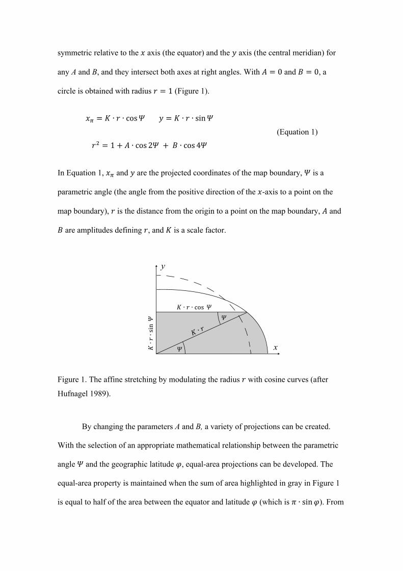
symmetric relative to the 𝑥 axis (the equator) and the 𝑦 axis (the central meridian) for

any A and B, and they intersect both axes at right angles. With 𝐴 = 0 and 𝐵 = 0, a

circle is obtained with radius 𝑟 = 1 (Figure 1).

𝑥! = 𝐾 ∙ 𝑟 ∙ cos𝛹 𝑦 = 𝐾 ∙ 𝑟 ∙ sin𝛹

𝑟! = 1+ 𝐴 ∙ cos 2𝛹 + 𝐵 ∙ cos 4𝛹

(Equation 1)

In Equation 1, 𝑥! and 𝑦 are the projected coordinates of the map boundary, 𝛹 is a

parametric angle (the angle from the positive direction of the 𝑥-axis to a point on the

map boundary), 𝑟 is the distance from the origin to a point on the map boundary, 𝐴 and

𝐵 are amplitudes defining 𝑟, and 𝐾 is a scale factor.

Figure 1. The affine stretching by modulating the radius 𝑟 with cosine curves (after

Hufnagel 1989).

By changing the parameters A and B, a variety of projections can be created.

With the selection of an appropriate mathematical relationship between the parametric

angle 𝛹 and the geographic latitude 𝜑, equal-area projections can be developed. The

equal-area property is maintained when the sum of area highlighted in gray in Figure 1

is equal to half of the area between the equator and latitude 𝜑 (which is 𝜋 ∙ sin𝜑). From

y

x

this condition one can derive the relation shown in Equation 2. Equation 3 is identical to

Equation 2, but Hufnagel eliminates 𝑟! using Equation 1 (Hufnagel 1989). In Equations

2 and 3, 𝜑 is the geographic latitude; 𝛹, 𝑟, 𝐴, 𝐵, and 𝐾 are defined as above.

𝜋 ∙ sin𝜑 =𝐾!

2 𝑟!𝑑𝛹!

!+𝐾!

2 𝑟! ∙ sin𝛹 ∙ cos𝛹

= 𝐾!

4 2 𝑟!𝑑𝛹 + 𝑟!sin2𝛹!

!

=𝐾!

4 2𝛹 + 𝐴 ∙ sin2𝛹 +𝐵2 sin4𝛹 + 𝑟! ∙ sin2𝛹

(Equation 2)

𝜋 ∙ sin𝜑 = 𝐾!

4 2𝛹 + 1+ 𝐴 −𝐵2 sin2𝛹 +

𝐴 + 𝐵2 sin4𝛹

+𝐵2 sin6𝛹

(Equation 3)

When 𝜑 = 90°, the corresponding 𝛹 in Equation 3 is the maximum parametric

angle 𝛹!"#. For 𝛹!"# = 90°, poles are represented with points. When 𝛹!"# is smaller

than 90°, projections have pole lines. Appendix 1 proves that when 𝛹!"# approaches 0,

the Hufnagel projection transforms into an equal-area cylindrical projection.

The value of the constant 𝐾 in Equations 1, 2, and 3 can be obtained from

Equation 3 by setting 𝜑 = 90°, 𝛹 = 𝛹!"#, and using the selected amplitudes 𝐴 and 𝐵

(see also Equation 7). To project the longitude 𝜆, the 𝑥-coordinate of the antimeridian is

multiplied by 𝜆 𝜋 (Equation 4) (Hufnagel 1989).

𝑥 = !!∙ 𝑥! = 𝐾 ∙ !

!∙ 𝑟 ∙ cos𝛹 (Equation 4)

The final step in Hufnagel’s derivation is an equal-area stretching applied to the

projected 𝑥- and 𝑦-coordinates. The stretching factor 𝐶 adjusts the map to the equator-

to-central meridian ratio desired by the cartographer (Equation 5). The factor C is

computed with Equation 6, where 𝛼 is the equator-to-central meridian ratio, and 𝛹!"# is

the maximum parametric angle. 𝐾 is computed from 𝐴, 𝐵, and 𝛹!"# with Equation 7.

𝑥 =𝐾 ∙ 𝐶𝜋 ∙ 𝜆 ∙ 𝑟 ∙ cos𝛹

(Equation 5)

𝑦 =𝐾𝐶 ∙ 𝑟 ∙ sin𝛹

𝐶! = 𝛼 ∙ sin𝛹!"# ∙!!!∙!"# !!!"#!!∙!"# !!!"#

!!!!! (Equation 6)

𝐾! = !!

!∙!!"#! !!!!!! ⋅!"# !!!"#!!!!! ⋅!"# !!!"#! !!⋅!"# !!!"#

(Equation 7)

Using Hufnagel’s derivation approach, the Mollweide projection is created by

first setting the amplitude factors 𝐴 and 𝐵 to 0, which results in a circular map

boundary. Then, the equal-area condition is applied to the circle using Equation 3 to

compute a parametric angle 𝛹 for each latitude 𝜑. The maximum parametric angle

𝛹!"# is set to 90°, because the Mollweide projection represents poles as points. And

finally, equal-area stretching with the factor 𝐶 = 2 (Equation 6) is applied to set the

equator-to-central meridian ratio 𝛼.to 2. Computational techniques are detailed in the

next section.

Tobler’s hyperelliptical projection family also includes the Mollweide projection

(Tobler 1973). However, the Tobler and Hufnagel’s projection families are

parameterized differently and have considerably different characteristics. Tobler uses a

family of curves called the hyperellipse, while Hufnagel uses a family of curves that has

no particular name. Unlike Tobler’s hyperellipses, Hufnagel’s curves have inflection

points, which results in a greater diversity in his projection family. As a practical matter

for computation, Hufnagel’s development also does not require numerical integration.

Some aspects of Hufnagel’s derivation are similar to Wagner’s area-preserving

transformation method called Umbeziffern, meaning renumbering (Wagner 1931, 1932,

1941, 1949, 1962). With the parametric angle 𝛹, new latitude values are computed, and

the map is adjusted to the preferred equator-to-central meridian ratio with the stretching

factor 𝐶.

Algorithms for the Hufnagel projection family

Individual members of Hufnagel’s projection family are created by configuring four

parameters: 𝐴 ∈ −1,1 , 𝐵 ∈ −1,1 , 𝛹!"# ∈ 0, !!

, and 𝐶, which is a stretching factor

that adjusts the map to the preferred equator-to-central meridian ratio. This section

details algorithmic steps for applying the parameters.

Direct equations for transforming spherical coordinates to plane Cartesian

coordinates do not exist for the Hufnagel projection family. To compute a parametric

angle 𝛹 for a corresponding latitude 𝜑 with Equation 3, an iteration procedure has to be

used. This is a well-known characteristic of the Mollweide projection (Mollweide 1805;

Snyder 1987, 1993) and the Eckert IV projection (Eckert 1906; Snyder 1987, 1993).

Using the Newton-Raphson method, the iteration process to find 𝛹 for a given latitude

𝜑 is as follows:

(1) Selection of a seed value 𝛹! for the unknown parametric angle 𝛹.

(2) Correction 𝛥𝛹:

𝛥𝛹 =!!

! !∙!!! !!!!!! ⋅!"# !!!!!!!! ⋅!"# !!!! !!⋅!"# !!! !! !"#!

!!! !! !!!!!! ⋅!"# !!!! !!! ⋅!"# !!!! !!! ⋅!"# !!!

(Equation 8)

(3) Improved value of the parametric angle: 𝛹!!! = 𝛹! − 𝛥𝛹

The calculation is repeated until 𝛥𝛹 < 𝜀 (a small threshold value). The

selection of a seed value for the parametric angle in step 1 is critical for the iterative

procedure to converge. We found no heuristic for a seed value that works across all

parameterizations of the projection. Therefore, we build three lookup tables, each with

the same size (we used 101 elements each). The first table contains linearly increasing

values of the parametric angle 𝛹 ∈ 0,𝛹!"# . It serves as an “index” into the other two

tables, one of which goes forward to the 𝑦 value computed from 𝛹, and the other of

which goes backward to the 𝜑 value computed from the same 𝛹. The tables represent

the relationship between 𝛹, 𝑦, and 𝜑 given fixed A, B, C, and 𝛹!"#. For a given 𝛹

appearing in the first table, the corresponding 𝑦 value and 𝜑 value appear at the same

index in their own respective tables. We index off of 𝛹 rather than off of 𝜑 or 𝑦 in order

to avoid having to iterate when calculating the tables, since 𝑦 and 𝜑 both can be

calculated in closed form from 𝛹. Algorithm 1 presents pseudocode for the

initialization of the lookup tables (with the number of elements equal to 𝑇𝑎𝑏𝑙𝑒𝑆𝑖𝑧𝑒).

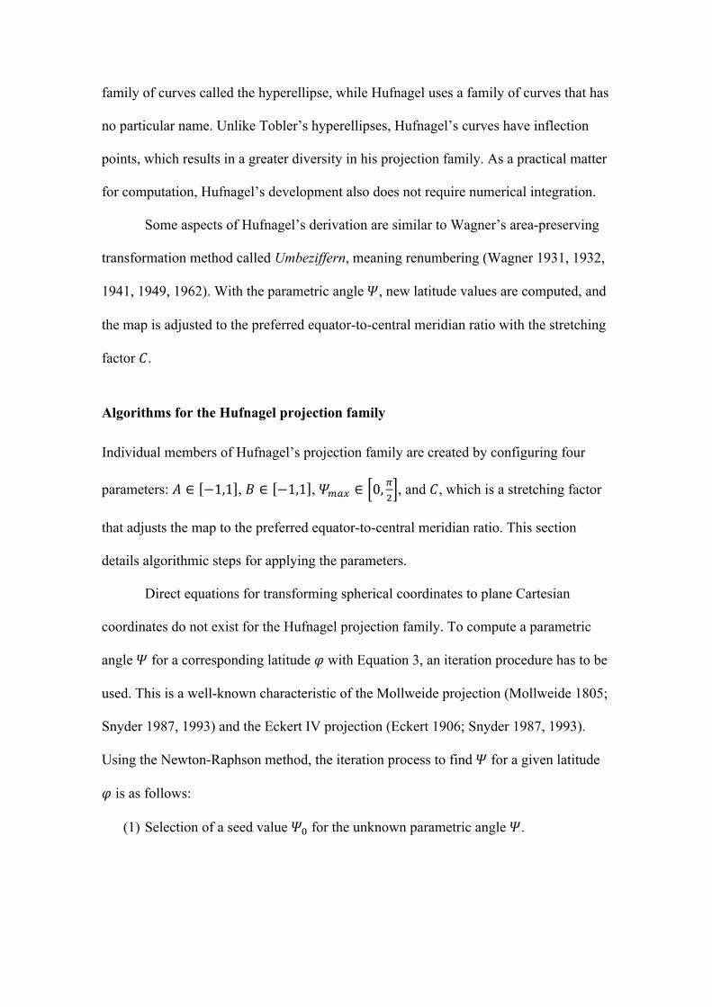
Algorithm 1. Initialization of the lookup tables 1: for 𝑖 ∈ 0,𝑇𝑎𝑏𝑙𝑒𝑆𝑖𝑧𝑒 − 1 do 2: 𝛹 = !∙!!"#

!"#$%&'(%!!

3: if 𝑖 = 0 then 4: 𝜑 = 0 5: else if 𝑖 = (𝑇𝑎𝑏𝑙𝑒𝑆𝑖𝑧𝑒 − 1) then 6: 𝜑 = 90° 7: else 8: 𝜑 from Equation 3 9: end if 10: 𝑟 from Equation 1 11: 𝑦 from Equation 5 12: if 𝑖 > 0 then 13: if 𝑦 < 𝑦𝑇𝑎𝑏𝑙𝑒[𝑖 − 1] or 𝜑 < 𝑙𝑎𝑡𝑖𝑡𝑢𝑑𝑒𝑇𝑎𝑏𝑙𝑒[𝑖 − 1] then 14: raise folding graticule exception 15: end if 16: end if 17: 𝑝𝑎𝑟𝑎𝑚𝐴𝑛𝑔𝑙𝑒𝑇𝑎𝑏𝑙𝑒 𝑖 = 𝛹 18: 𝑙𝑎𝑡𝑖𝑡𝑢𝑑𝑒𝑇𝑎𝑏𝑙𝑒 𝑖 = 𝜑 19: 𝑦𝑇𝑎𝑏𝑙𝑒 𝑖 = 𝑦 20: end for

Algorithm 1 uses the lookup table for the 𝑦-coordinate to identify combinations

of the parameters A, B, 𝛹!"# that result in y values failing to increase monotonically

with φ, in which case an exception is raised (lines 13–15). In other words, δy/δφ goes

negative, causing some higher latitudes to end up closer to the equator on the map than

lower latitudes do. This could be detected more analytically but was not deemed worth

the effort; given the size of the look-up tables, only a tiny uncertainty remains in

detecting failure of monotonicity while also yielding robust seed values.

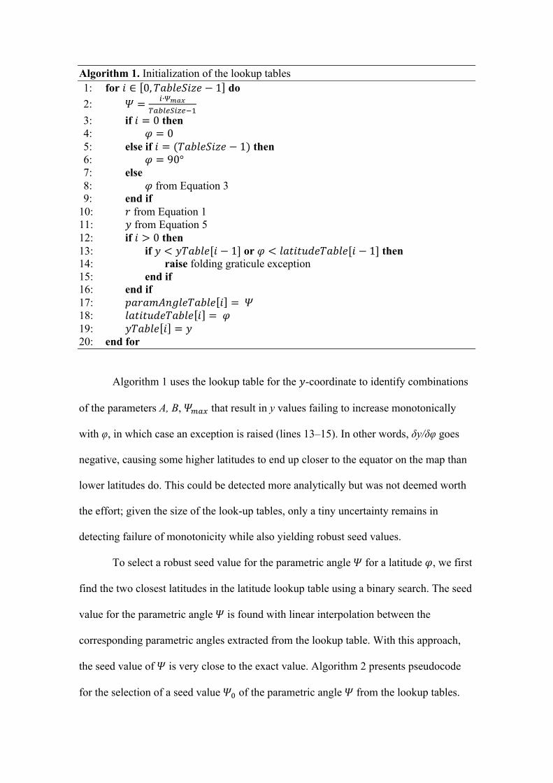
To select a robust seed value for the parametric angle 𝛹 for a latitude 𝜑, we first

find the two closest latitudes in the latitude lookup table using a binary search. The seed

value for the parametric angle 𝛹 is found with linear interpolation between the

corresponding parametric angles extracted from the lookup table. With this approach,

the seed value of 𝛹 is very close to the exact value. Algorithm 2 presents pseudocode

for the selection of a seed value 𝛹! of the parametric angle 𝛹 from the lookup tables.

Algorithm 2. Finding seed value 𝛹! of the parametric angle 𝛹 Input: 𝜑 1: 𝑖!"# = 0 2: 𝑖!"#= 𝑇𝑎𝑏𝑙𝑒𝑆𝑖𝑧𝑒 3: repeat 4: 𝑖!"# =

!!"#!!!"#!

5: if 𝑖!"# equals 𝑖!"# then 6: break loop 7: else if 𝜑 > 𝑙𝑎𝑡𝑖𝑡𝑢𝑑𝑒𝑇𝑎𝑏𝑙𝑒 𝑖!"# then 8: 𝑖!"# = 𝑖!"# 9: else 10: 𝑖!"# = 𝑖!"# 11: end if 12: end loop 13: 𝜑! = 𝑙𝑎𝑡𝑖𝑡𝑢𝑑𝑒𝑇𝑎𝑏𝑙𝑒 𝑖!"# 14: 𝜑! = 𝑙𝑎𝑡𝑖𝑡𝑢𝑑𝑒𝑇𝑎𝑏𝑙𝑒 𝑖!"# + 1 15: 𝑤𝑒𝑖𝑔ℎ𝑡 = ! !!!

!!!!!

16: 𝛹! = 𝑝𝑎𝑟𝑎𝑚𝐴𝑛𝑔𝑙𝑒𝑇𝑎𝑏𝑙𝑒[𝑖!"#] 17: 𝛹! = 𝑝𝑎𝑟𝑎𝑚𝐴𝑛𝑔𝑙𝑒𝑇𝑎𝑏𝑙𝑒[𝑖!"# + 1] 18: 𝛹! = 𝑤𝑒𝑖𝑔ℎ𝑡 ∙ 𝛹! −𝛹! +𝛹! 19: return 𝜑 < 0 ? −𝛹! : 𝛹!

After calculating the parametric angle 𝛹, the Cartesian coordinates are obtained

with Equation 5. Algorithm 3 presents pseudocode for the computation of Cartesian

coordinates from spherical coordinates.

Algorithm 3. Projecting spherical coordinates to Cartesian coordinates Inputs: 𝜆 and 𝜑 1: Find seed value 𝛹!. (Algorithm 2) 2: repeat 3: 𝛥𝛹!"#$%&'(% of Equation 8 4: if 𝛥𝛹!"#$%&'(% < 𝜀 5: break loop 6: end if 7: 𝛥𝛹!"#$%&#'($) of Equation 8 8: 𝛥𝛹 = !!"#$%&'(%

!!!"#$%&#'($)

9: 𝛹!!! = 𝛹! − Δ𝛹 10: end loop 11: 𝑟 with Equation 1 12: 𝑥 with Equation 5 13: 𝑦 with Equation 5 14: return [𝑥,𝑦]

The Mollweide, Eckert IV, and Wagner IV projections have direct reverse equations.

However, general members of the Hufnagel projection family require an iteration

procedure. The Newton-Raphson method can be used with Equation 9 to find the

correction ∆𝛹 of the parametric angle for a given 𝑦-coordinate (r is defined in Equation

1).

𝛥𝛹 =!!∙!"#!!!!

!∙!!

!

!"# !!!∙ !!!!!!! !!!!! ∙!"# !!! ! !!∙!"# !!! (Equation 9)

For the selection of a seed value 𝛹!, the parametric angle and 𝑦-coordinate look-up

tables are used. The algorithm used to find the seed value is similar to Algorithm 2,

except the 𝑦-coordinate is used instead of the latitude value. After the parametric angle

𝛹 is computed, the latitude can be obtained from Equation 3 and the longitude is

computed from Equation 5. Algorithm 4 shows pseudocode for determining spherical

coordinates from Cartesian coordinates.

Algorithm 4. Projecting Cartesian coordinates to spherical coordinates Inputs: 𝑥 and 𝑦 1: Find seed value 𝛹!. (Algorithm 2, using 𝑦-coordinate look-up table) 2: repeat 3: 𝛥𝛹!"#$%&'(% of Equation 9 4: if 𝛥𝛹!"#$%&'(% < 𝜀 5: break loop 6: end if 7: 𝛥𝛹!"#$%&#'($) of Equation 9 8: 𝛥𝛹 = !!"#$%&'(%

!!!"#$%&#'($)

9: 𝛹!!! = 𝛹! − Δ𝛹 10: end loop 11: 𝑟 with Equation 1 12: 𝜑 with Equation 3 13: 𝜆 with Equation 5 14: return [𝜆 ,𝜑]

Hufnagel’s eight projections

Hufnagel introduced eight new projections for world maps, which are all members of

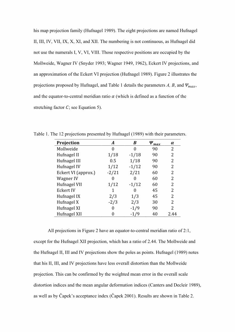
his map projection family (Hufnagel 1989). The eight projections are named Hufnagel

II, III, IV, VII, IX, X, XI, and XII. The numbering is not continuous, as Hufnagel did

not use the numerals I, V, VI, VIII. Those respective positions are occupied by the

Mollweide, Wagner IV (Snyder 1993; Wagner 1949, 1962), Eckert IV projections, and

an approximation of the Eckert VI projection (Hufnagel 1989). Figure 2 illustrates the

projections proposed by Hufnagel, and Table 1 details the parameters A, B, and 𝛹!"#,

and the equator-to-central meridian ratio 𝛼 (which is defined as a function of the

stretching factor 𝐶; see Equation 5).

Table 1. The 12 projections presented by Hufnagel (1989) with their parameters.

Projection 𝑨 𝑩 𝜳𝒎𝒂𝒙 𝜶Mollweide 0 0 90 2HufnagelII 1/18 -1/18 90 2HufnagelIII 0.5 1/18 90 2HufnagelIV 1/12 -1/12 90 2EckertVI(approx.) -2/21 2/21 60 2WagnerIV 0 0 60 2HufnagelVII 1/12 -1/12 60 2EckertIV 1 0 45 2HufnagelIX 2/3 1/3 45 2HufnagelX -2/3 2/3 30 2HufnagelXI 0 -1/9 90 2HufnagelXII 0 -1/9 40 2.44

All projections in Figure 2 have an equator-to-central meridian ratio of 2:1,

except for the Hufnagel XII projection, which has a ratio of 2.44. The Mollweide and

the Hufnagel II, III and IV projections show the poles as points. Hufnagel (1989) notes

that his II, III, and IV projections have less overall distortion than the Mollweide

projection. This can be confirmed by the weighted mean error in the overall scale

distortion indices and the mean angular deformation indices (Canters and Decleir 1989),

as well as by Čapek’s acceptance index (Čapek 2001). Results are shown in Table 2.

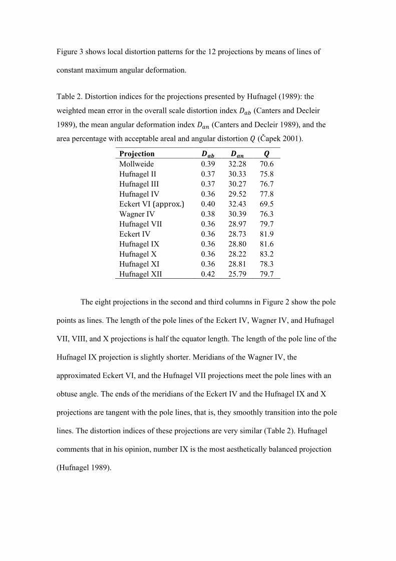
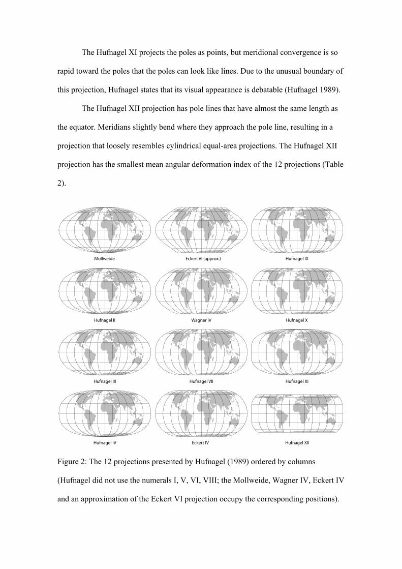
Figure 3 shows local distortion patterns for the 12 projections by means of lines of

constant maximum angular deformation.

Table 2. Distortion indices for the projections presented by Hufnagel (1989): the

weighted mean error in the overall scale distortion index 𝐷!" (Canters and Decleir

1989), the mean angular deformation index 𝐷!" (Canters and Decleir 1989), and the

area percentage with acceptable areal and angular distortion 𝑄 (Čapek 2001).

Projection 𝑫𝒂𝒃 𝑫𝒂𝒏 𝑸 Mollweide 0.39 32.28 70.6 Hufnagel II 0.37 30.33 75.8 Hufnagel III 0.37 30.27 76.7 Hufnagel IV 0.36 29.52 77.8 Eckert VI (approx.) 0.40 32.43 69.5 Wagner IV 0.38 30.39 76.3 Hufnagel VII 0.36 28.97 79.7 Eckert IV 0.36 28.73 81.9 Hufnagel IX 0.36 28.80 81.6 Hufnagel X 0.36 28.22 83.2 Hufnagel XI 0.36 28.81 78.3 Hufnagel XII 0.42 25.79 79.7

The eight projections in the second and third columns in Figure 2 show the pole

points as lines. The length of the pole lines of the Eckert IV, Wagner IV, and Hufnagel

VII, VIII, and X projections is half the equator length. The length of the pole line of the

Hufnagel IX projection is slightly shorter. Meridians of the Wagner IV, the

approximated Eckert VI, and the Hufnagel VII projections meet the pole lines with an

obtuse angle. The ends of the meridians of the Eckert IV and the Hufnagel IX and X

projections are tangent with the pole lines, that is, they smoothly transition into the pole

lines. The distortion indices of these projections are very similar (Table 2). Hufnagel

comments that in his opinion, number IX is the most aesthetically balanced projection

(Hufnagel 1989).

The Hufnagel XI projects the poles as points, but meridional convergence is so

rapid toward the poles that the poles can look like lines. Due to the unusual boundary of

this projection, Hufnagel states that its visual appearance is debatable (Hufnagel 1989).

The Hufnagel XII projection has pole lines that have almost the same length as

the equator. Meridians slightly bend where they approach the pole line, resulting in a

projection that loosely resembles cylindrical equal-area projections. The Hufnagel XII

projection has the smallest mean angular deformation index of the 12 projections (Table

2).

Figure 2: The 12 projections presented by Hufnagel (1989) ordered by columns

(Hufnagel did not use the numerals I, V, VI, VIII; the Mollweide, Wagner IV, Eckert IV

and an approximation of the Eckert VI projection occupy the corresponding positions).

Hufnagel XII

Hufnagel XI

Hufnagel X

Hufnagel IX

Eckert IV

Hufnagel VII

Wagner IV

Eckert VI (approx.)

Hufnagel IV

Hufnagel III

Hufnagel II

Mollweide

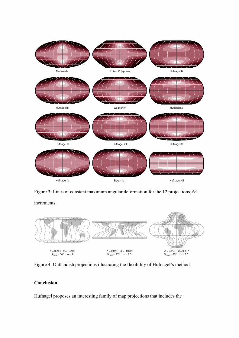
Figure 3: Lines of constant maximum angular deformation for the 12 projections, 6°

increments.

Figure 4: Outlandish projections illustrating the flexibility of Hufnagel’s method.

Conclusion

Hufnagel proposes an interesting family of map projections that includes the

Hufnagel XII

Hufnagel XI

Hufnagel X

Hufnagel IX

Eckert IV

Hufnagel VII

Wagner IV

Eckert VI (approx.)

Hufnagel IV

Hufnagel III

Hufnagel II

Mollweide

A = 0.213 B = –0.402Ψmax = 56º α = 2

A = 0.071 B = –0.835Ψmax = 33º α = 1.5

A = 0.155 B = 0.437Ψmax = 80º α = 1.5

Mollweide, Eckert IV, and Wagner IV projections as special cases. Additional

projections can be created by varying the parameters A, B, and 𝛹!"#, and the equator-

to-central meridian ratio of the map. Hufnagel’s method is very flexible and allows for

creating a variety of equal-area pseudocylindric projections. Many parameter

combinations result in absurd distortion characteristics or folding graticules that are of

little value for practical map making (Figure 4). We explored valid ranges of the A, B,

and 𝛹!"# parameters that result in non-folded graticules, but the distribution pattern of

valid combinations is very irregular and difficult to visualize. Many projections in this

pseudocylindric projection family have nevertheless reasonable distortion properties,

and seem to be useful for a variety of equal-area world maps. We recommend using a

specialized graphical user interface coupled with a WYSIWYG map visualization for

selecting projection parameters when creating a customized Hufnagel projection (an

example for the Hufnagel projection family is available at

http://projectionwizard.org/Hufnagel.html.

The Hufnagel projections will be available in the next version of the Geocart

software (https://www.mapthematics.com). The computational method and algorithms

presented in this article were implemented in the open-source Java Map Projection

Library (https://github.com/OSUCartography/JMapProjLib). We hope that this

contribution will help Hufnagel’s projection family find its place in other cartographic

projection libraries and software applications, and eventually on world maps.

Acknowledgements

The authors would like to thank Richard Čapek, Tomas Bayer (Charles University,

Prague), Jan D. Bláha (Jan Evangelista Purkyně University, Ústí nad Labem, Czechia),

and Rolf Böhm (Ingenieurbüro für Kartographie, Bad Schandau, Germany) for their

help and comments. The support of Esri, Inc. is greatly acknowledged. We also thank

Abby Metzger and Gareth Baldrica-Franklin, Oregon State University, for editing this

text and figures, and the anonymous reviewers for their valuable comments.

References

Canters, F. 2002. Small-Scale Map Projection Design. London: Taylor & Francis.

Canters, F., Decleir, H., 1989. The World in Perspective: A Directory of World Map

Projections. John Wiley and Sons, Chichester, 181 pp.

Čapek, R. 2001. Which is the best projection for the world map? In: Proceedings of the

20th International Cartographic Conference, Beijing, China, August 6–10, 2001.

Vol. 5, pp. 3084-93.

Eckert, M., 1906. Neue Entwürfe für Erdkarten. Petermanns Mitteilungen, 52 (5): 97–

109.

Hufnagel, H. 1989. Ein System unecht-zylindrischer Kartennetze für Erdkarten.

Kartographische Nachrichten, 39 (3): 89–96.

Jenny, B., Patterson, T., Hurni L. 2008. Flex Projector—Interactive software for

designing world map projections. Cartographic Perspectives, 59: 12–27.

Jenny, B. 2012. Adaptive composite map projections. IEEE Transactions on

Visualization and Computer Graphics (Proceedings Scientific Visualization /

Information Visualization 2012), 18 (12): 575–2582.

Mollweide, K.B., 1805. Über die vom Prof. Schmidt in Giessen in der zweyten

Abtheilung seines Handbuchs der Naturlehre S. 595 angegebene Projection der

Halbkugelfläche. Zach’s Monatliche Correspondenz zur Beförderung der Erd-

und Himmels-Kunde, 8: 152–163.

Šavrič, B., Jenny, B., White, D., Strebe D. R. 2015. User preferences for world map

projections. Cartography and Geographic Information Science, 42 (5): 398–409.

Snyder, J.P., 1987. Map projections: A Working Manual. US Geological Survey,

Washington, DC, 383 pp.

Snyder, J.P., 1993. Flattening the Earth. Two Thousand Years of Map Projections.

Chicago & London: University of Chicago Press.

Tobler, W. R. 1973. The hyperelliptical and other new pseudo cylindrical equal area

map projections. Journal of Geophysical Research, 78 (11): 1753–1759.

Wagner, K.H., 1931. Die unechten Zylinderprojektionen: Ihre Anwendung und ihre

Bedeutung für die Praxis. Doctoral dissertation. Mathematisch-

Naturwissenschaftliche Fakultät, University of Hamburg.

Wagner, K.H., 1932. Die unechten Zylinderprojektionen. Aus dem Archiv der

Deutschen Seewarte, 51 (4), 68.

Wagner, K.H., 1941. Neue ökumenische Netzentwürfe für die kartographische Praxis.

Jahrbuch der Kartographie, 176–202.

Wagner, K.H., 1949. Kartographische Netzentwürfe. Leipzig: Bibliographisches

Institut.

Wagner, K.H., 1962. Kartographische Netzentwürfe. 2nd ed. Mannheim:

Bibliographisches Institut.

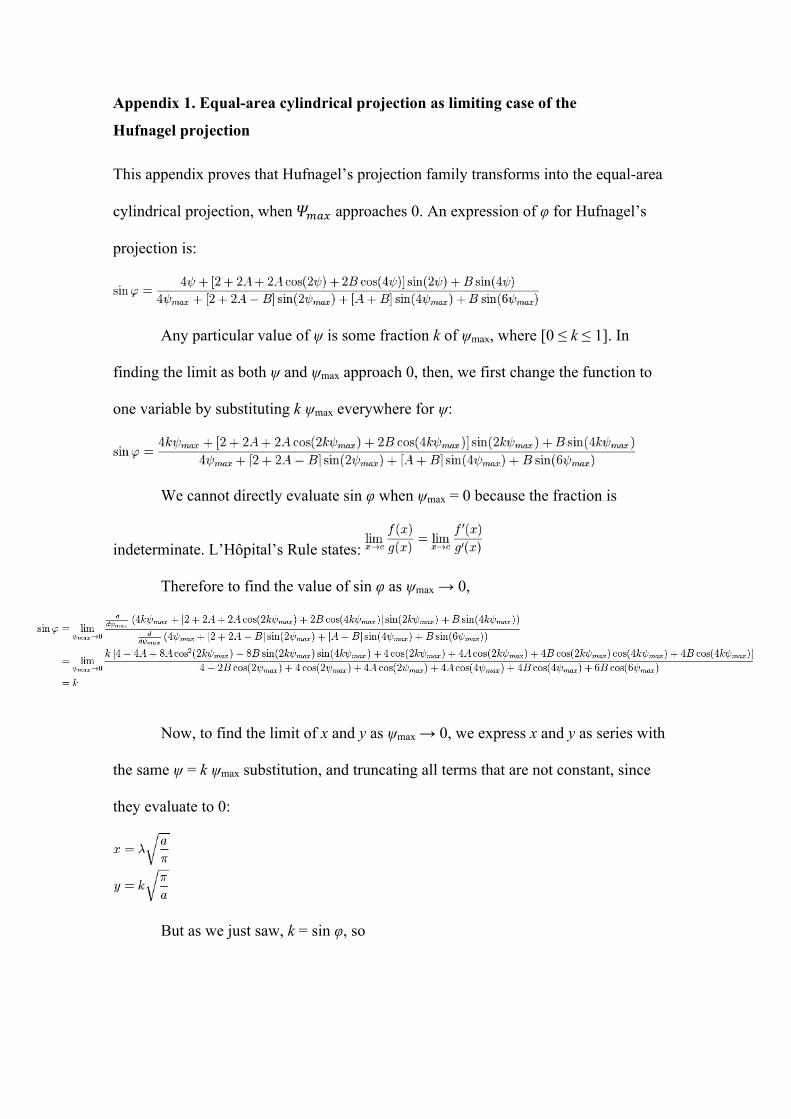
Appendix 1. Equal-area cylindrical projection as limiting case of the

Hufnagel projection

This appendix proves that Hufnagel’s projection family transforms into the equal-area

cylindrical projection, when 𝛹!"# approaches 0. An expression of φ for Hufnagel’s

projection is:

Any particular value of ψ is some fraction k of ψmax, where [0 ≤ k ≤ 1]. In

finding the limit as both ψ and ψmax approach 0, then, we first change the function to

one variable by substituting k ψmax everywhere for ψ:

We cannot directly evaluate sin φ when ψmax = 0 because the fraction is

indeterminate. L’Hôpital’s Rule states:

Therefore to find the value of sin φ as ψmax → 0,

Now, to find the limit of x and y as ψmax → 0, we express x and y as series with

the same ψ = k ψmax substitution, and truncating all terms that are not constant, since

they evaluate to 0:

But as we just saw, k = sin φ, so

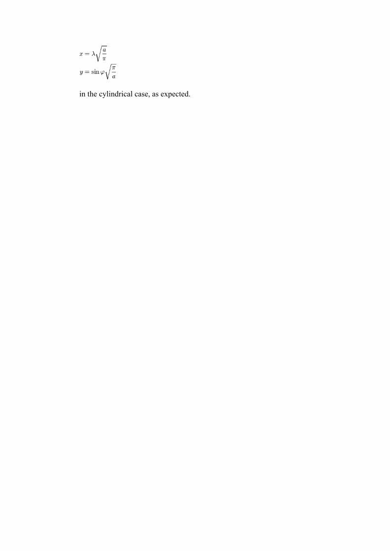
in the cylindrical case, as expected.