work zone impact and strategy estimator (wise) software
TRANSCRIPT

SHRP 2 Renewal Project R11
Work Zone Impact and Strategy
Estimator (WISE) Software Validation and Pilot Tests

SHRP 2 Renewal Project R11
Work Zone Impact and Strategy Estimator (WISE) Software Validation and Pilot Tests
Dane Ismart, Principal Investigator The Louis Berger Group, Inc.
Washington, D.C.
TRANSPORTATION RESEARCH BOARD Washington, D.C.
2014 www.TRB.org

© 2014 National Academy of Sciences. All rights reserved. ACKNOWLEDGMENT This work was sponsored by the Federal Highway Administration in cooperation with the American Association of State Highway and Transportation Officials. It was conducted in the second Strategic Highway Research Program, which is administered by the Transportation Research Board of the National Academies. COPYRIGHT INFORMATION Authors herein are responsible for the authenticity of their materials and for obtaining written permissions from publishers or persons who own the copyright to any previously published or copyrighted material used herein. The second Strategic Highway Research Program grants permission to reproduce material in this publication for classroom and not-for-profit purposes. Permission is given with the understanding that none of the material will be used to imply TRB, AASHTO, or FHWA endorsement of a particular product, method, or practice. It is expected that those reproducing material in this document for educational and not-for-profit purposes will give appropriate acknowledgment of the source of any reprinted or reproduced material. For other uses of the material, request permission from SHRP 2. NOTICE The project that is the subject of this document was a part of the second Strategic Highway Research Program, conducted by the Transportation Research Board with the approval of the Governing Board of the National Research Council. The Transportation Research Board of the National Academies, the National Research Council, and the sponsors of the second Strategic Highway Research Program do not endorse products or manufacturers. Trade or manufacturers’ names appear herein solely because they are considered essential to the object of the report. DISCLAIMER The opinions and conclusions expressed or implied in this document are those of the researchers who performed the research. They are not necessarily those of the second Strategic Highway Research Program, the Transportation Research Board, the National Research Council, or the program sponsors. The information contained in this document was taken directly from the submission of the authors. This material has not been edited by the Transportation Research Board. SPECIAL NOTE: This document IS NOT an official publication of the second Strategic Highway Research Program, the Transportation Research Board, the National Research Council, or the National Academies.

The National Academy of Sciences is a private, nonprofit, self-perpetuating society of distinguished scholars engaged in scientific and engineering research, dedicated to the furtherance of science and technology and to their use for the general welfare. On the authority of the charter granted to it by Congress in 1863, the Academy has a mandate that requires it to advise the federal government on scientific and technical matters. Dr. Ralph J. Cicerone is president of the National Academy of Sciences.
The National Academy of Engineering was established in 1964, under the charter of the National Academy of Sciences, as a parallel organization of outstanding engineers. It is autonomous in its administration and in the selection of its members, sharing with the National Academy of Sciences the responsibility for advising the federal government. The National Academy of Engineering also sponsors engineering programs aimed at meeting national needs, encourages education and research, and recognizes the superior achievements of engineers. Dr. C. D. (Dan) Mote, Jr., is president of the National Academy of Engineering.
The Institute of Medicine was established in 1970 by the National Academy of Sciences to secure the services of eminent members of appropriate professions in the examination of policy matters pertaining to the health of the public. The Institute acts under the responsibility given to the National Academy of Sciences by its congressional charter to be an adviser to the federal government and, upon its own initiative, to identify issues of medical care, research, and education. Dr. Victor J. Dzau is president of the Institute of Medicine.
The National Research Council was organized by the National Academy of Sciences in 1916 to associate the broad community of science and technology with the Academy’s purposes of furthering knowledge and advising the federal government. Functioning in accordance with general policies determined by the Academy, the Council has become the principal operating agency of both the National Academy of Sciences and the National Academy of Engineering in providing services to the government, the public, and the scientific and engineering communities. The Council is administered jointly by both Academies and the Institute of Medicine. Dr. Ralph J. Cicerone and Dr. C.D. (Dan) Mote, Jr., are chair and vice chair, respectively, of the National Research Council. The Transportation Research Board is one of six major divisions of the National Research Council. The mission of the Transportation Research Board is to provide leadership in transportation innovation and progress through research and information exchange, conducted within a setting that is objective, interdisciplinary, and multimodal. The Board’s varied activities annually engage about 7,000 engineers, scientists, and other transportation researchers and practitioners from the public and private sectors and academia, all of whom contribute their expertise in the public interest. The program is supported by state transportation departments, federal agencies including the component administrations of the U.S. Department of Transportation, and other organizations and individuals interested in the development of transportation. www.TRB.org
www.national-academies.org
Contents 1 Author Acknowledgments
2 Summary
5 CHAPTER 1 Introduction 5 Introduction 6 Selection of Validation Sites 6 Selection of Pilot Sites 8 CHAPTER 2 Iowa Validation Process and Results 8 Introduction 11 Summary of Testing Procedures and Scenarios 13 Synopsis of Validation Results 19 CHAPTER 3 Phoenix, Arizona, Validation Test Deployment 19 Introduction 19 Summary of Testing Procedures and Scenarios 23 Synopsis of Validation Results 28 CHAPTER 4 Wise Pilot Test Deployment: Orlando, Florida 28 Introduction 28 Summary of Testing Procedures and Scenarios 31 Synopsis of Pilot Test Results 35 CHAPTER 5 Pilot Test Deployment: Worcester, Massachusetts 35 Introduction 35 Summary of Testing Procedures 38 Synopsis of Scenarios and Pilot Test Results 44 CHAPTER 6 Conclusion and Summary Recommendations 45 Summary of Phase 4 Findings and Recommendations 47 APPENDIX A Validation Test Project Descriptions 47 Part 1. Iowa DOT I-235 Project Description 50 Part 2. Phoenix, Arizona, Project Descriptions

57 APPENDIX B Pilot Test Project Descriptions 57 Orlando, Florida, Proposed Project Descriptions 58 APPENDIX C Transcad GISDK Scripts 58 Part 1. Iowa Validation TransCAD GISDK Script 62 Part 2. Phoenix, Arizona, TransCAD GISDK Script 66 Part 3. Orlando, Florida, TransCAD GISDK Script 70 Part 4. Worcester, Massachusetts, TransCAD GISDK Script

AUTHOR ACKNOWLEDGMENTS This work was sponsored by the Federal Highway Administration in cooperation with the American Association of State Highway and Transportation Officials, and it was conducted in the second Strategic Highway Research Program, which is administered by the Transportation Research Board of the National Academies. The work on SHRP 2 R11 was led by a team from the Louis Berger Group, Inc., with Lawrence Pesesky, AICP, Principal in Charge; Dane Ismart, Principal Investigator; and Deborah Matherly, AICP, Project Management Coordinator, with extensive and essential research support as noted below.
The researchers and authors of this Phase 4 report are Dane Ismart, Principal Investigator, Orlando, Florida; Ed Bromage and Lindsay Bromage, E.J. Bromage LLC, Needham, Massachusetts; Dan Morgan, Caliper Corporation, Needham, Massachusetts; and Deborah Matherly, the Louis Berger Group, Inc., Washington, D.C.
The authors also gratefully acknowledge the contributions of the four validation and pilot test sites: Phil Mescher, Adam Shell, and Darla James, Des Moines, Iowa; Brent Cain, Phoenix, Arizona; Loreen Bobo, Orlando, Florida; and Mary Ellen Blunt, Central Massachusetts Regional Planning Commission, Worcester, Massachusetts.

SUMMARY Program managers within state departments of transportation (DOTs) and metropolitan planning organizations (MPOs) are charged with distilling a chaotic universe of identified renewal needs into a logically sequenced program of manageable projects over a period of years. In addition, program managers are tasked with sequencing programs of projects in ways that maximize available resources, minimize disruptions to the traveling public and to adjacent land uses, and recognize political priorities. Over the past several years, substantial progress has been made in the areas of performance measurement, maintenance of traffic, mitigation of congestion in work zones, and alternative contracting and construction techniques. All of this progress has been made in studies and planning designed to minimize, manage, and mitigate disruption to traffic and commerce arising from renewal programs. In application, however, performance measures are applied largely at the project level, and impacts are not analyzed at the program (mesoscopic) level. The products of this second Strategic Highway Research Program study project include a software tool that will assist program managers at DOTs and MPOs in sequencing programs of projects and also the training materials to apply this tool.
The Final Report for Phases 1, 2, and 3 documents the full literature review and research process and is available online at http://www.trb.org/Main/Blurbs/168143.aspx. Task 1 of the project identified the universe of published works that may be applicable to the products of this project. During the Task 2 literature analysis, 135 documents from Task 1 were identified as being “highly relevant” to this project and were reviewed to extract critical information. In Tasks 3, 4, and 5, a similar data set was extracted through interviews with DOTs, MPOs, and other key stakeholders. This allowed the research team (the Team) to draw comparisons and identify differences between literature and practice. The Team observed that the gap between the state of the art (identified in Tasks 1 and 2) and the state of the practice (identified in Tasks 3 and 4) is quite pronounced and varies widely across the country. Available software platforms with similar capabilities to those considered in this project were identified and analyzed in Phases 1, 2, and 3. The lessons learned from the Team’s review of the various software platforms and packages provided the basis and critical information for the WISE tool.
Phase 4 validation and pilot tests were conducted by a team of modelers completely independent from the initial developers of the WISE software in order to provide an objective assessment and realistic test of the developed tool on different networks and in different situations. The tests have identified strengths in the WISE tool as well as challenges that users will encounter in using the tool. It is recommended that the implementation challenges for users should be corrected in a future phase to facilitate wider dissemination and use of the positive features of the WISE tool.
WISE is envisioned to be used to develop and sequence programs of renewal projects in the Planning Module and to assist in the application of the “Work Zone Rule” in the Operation Module. The WISE tool includes both Planning and Operation Modules and may be applied over relatively large networks, or upon complex corridors, with some restrictions as identified below

that can be corrected in a future phase. The WISE software tool uses basic network geometry (link/node and number of lanes) and basic traffic volume information from virtually any platform once it is converted to a Network Explorer for Traffic Analysis (NEXTA) format. Detailed instructions for conversion of network and traffic data into NEXTA formats are included in the User Guide provided as part of this project. This report documents experiences, challenges, and potential user strategies to overcome (or work around) those challenges in converting existing networks to the required nonproprietary NEXTA format.
In the Planning Module, static assignment (user supplied or WISE supplied) is coupled with information about the planning characteristics of the program, a user-defined library of demand-based and duration-based renewal strategies, and basic project information. Optimal project sequencing is developed based on user and agency costs. Traffic diversion resulting from projects can be computed by WISE or entered manually for each project by the user. Later, in the Operation Module, operational software (TransModeler, the DynusT dynamic traffic assignment model, or another traffic simulation platform as chosen by the user) can compute a diversion of traffic based on more specific work zone information. The user can employ his or her choice of operational software at the microscopic (or macroscopic) level to model projects and identify traffic diversion and manually enter the diversion into the Planning Module to develop an optimized sequence of projects and construction strategies. The graphical user interface (GUI) includes a number of validation checks as well as user support features.
The WISE software has been further developed and improved in the validation and pilot tests in Phase 4 of this project, as documented in this report. Phase 4 has provided the opportunity to test and improve the stability and rigor of the WISE code and to identify deployment challenges and desirable improvements to increase the utility of the WISE tool. The User Guide and the Participant Workbook have undergone minor changes to reflect improvements in the software output. They will remain stand-alone documents; however, the User Guide is envisioned as a companion to the Participant Workbook, improving the user’s comfort with the functionality of WISE. Summary of Phase 4 Findings and Recommendations WISE was deliberately built on a platform of nonproprietary software to enable its free distribution. The underlying network platform, NEXTA, has substantial limitations that were not identified until the validation and pilot tests were undertaken. WISE was developed to work on a NEXTA network for the island of Guam, consisting of two-way streets and intersections, without highways, ramps, or one-way roads. Therefore, users are required to convert their existing network to a two-way configuration with intersections or develop such a “stick network” following the directions in the User Guide. A desirable future improvement would be to modify the WISE tool to interface directly with virtually any commercial or nonproprietary network system, rather than require users to convert their networks to meet the WISE specifications for a NEXTA network. This would enable WISE to easily evaluate large projects on Interstates and large corridors.

WISE considers a single construction project as occurring on a single highway segment. The software does not have the ability to consider that a construction project might involve numerous roadway segments. A second recommended improvement is to increase WISE’s flexibility in defining construction project scales in regard to highway segments.
WISE is limited in the number of zones and nodes that can be considered. A third recommended improvement is to increase the capacity of WISE to handle more zones.
Once a project is completed, the WISE program does not set the capacity back to 100%. In fact, some projects increase capacity, and the program does not have the ability to recognize that the capacity has increased. This may or may not affect the timing and optimization of project segments; this refinement represents a fourth recommendation for a future improvement.
The WISE tool is successful in setting optimized time frames for a set of work zone projects; it is successful in identifying user costs based on delay and diversion, plus agency costs for different projects. It is also successful in discerning between differing construction and public involvement strategies. However, the Planning Module estimates for diversion are not robust; user-supplied estimates of diversion will be better in most cases, and diversion estimates developed by running a microsimulation model will be even better. A fifth recommended improvement for a future version of WISE is additional testing and development for the diversion estimates, including feedback from the user’s network model, as described in the first recommendation.
Proprietary software developers may be able to expand and improve the operation of WISE. As currently designed, DOTs may find value in using WISE within the limits described, knowing its capabilities.

CHAPTER 1
Introduction WISE (Work Zone Impact and Strategy Estimator) is a planning tool designed to aid in the analysis of construction staging and construction mitigation analysis.
WISE is
• A bridge between macroscopic and microscopic models. • Designed to provide a sequencing of project construction. • A tool to help develop strategies to minimize impacts of renewal programs.
WISE is not
• A substitute for travel demand models. • A substitute for traffic simulation models.
WISE capabilities include
• The ability to evaluate impacts of multiple projects in a construction program upon a highway network.
• A decision support system to evaluate the impact of work zones and evaluate strategies to manage these impacts.
• A tool that requires minimal additional effort to conduct analyses.
There are two modules in WISE:
• A Planning Module, which is designed to develop a desirable construction program schedule over a planning horizon to manage, minimize, and mitigate impacts. The Planning Module can be used to test various strategies such as day/night construction, accelerated construction, and public information campaigns, employing WISE-default or user-supplied estimates of diversion, to estimate differences in user costs, total project costs, and the optimized timing sequence for projects.
• An Operation Module, which is designed to focus on “what-if” scenario analysis in which benefits/costs of various strategies are analyzed based upon dynamic traffic assignment. The full Operation Module is dependent upon the traffic operational software selected by the user. Traffic operational software can be labor-intensive to develop and calibrate. However, virtually any local or regional traffic simulation model can be used to input the locations of proposed projects
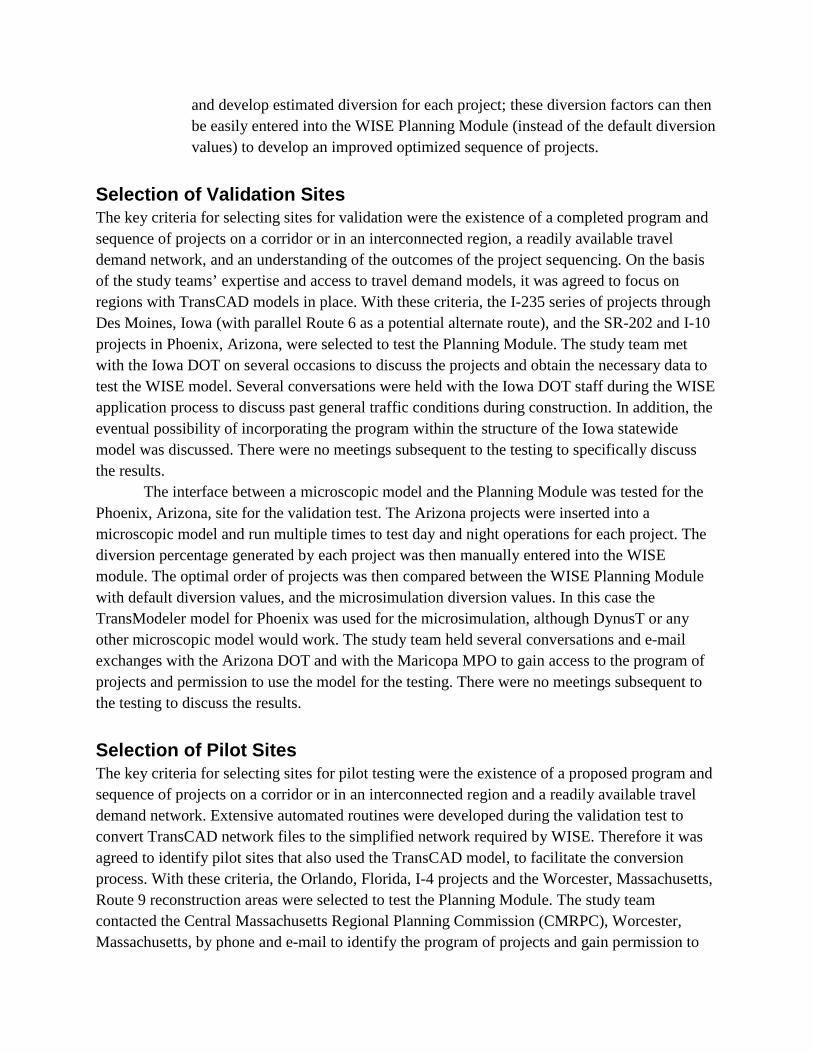
and develop estimated diversion for each project; these diversion factors can then be easily entered into the WISE Planning Module (instead of the default diversion values) to develop an improved optimized sequence of projects.
Selection of Validation Sites The key criteria for selecting sites for validation were the existence of a completed program and sequence of projects on a corridor or in an interconnected region, a readily available travel demand network, and an understanding of the outcomes of the project sequencing. On the basis of the study teams’ expertise and access to travel demand models, it was agreed to focus on regions with TransCAD models in place. With these criteria, the I-235 series of projects through Des Moines, Iowa (with parallel Route 6 as a potential alternate route), and the SR-202 and I-10 projects in Phoenix, Arizona, were selected to test the Planning Module. The study team met with the Iowa DOT on several occasions to discuss the projects and obtain the necessary data to test the WISE model. Several conversations were held with the Iowa DOT staff during the WISE application process to discuss past general traffic conditions during construction. In addition, the eventual possibility of incorporating the program within the structure of the Iowa statewide model was discussed. There were no meetings subsequent to the testing to specifically discuss the results.
The interface between a microscopic model and the Planning Module was tested for the Phoenix, Arizona, site for the validation test. The Arizona projects were inserted into a microscopic model and run multiple times to test day and night operations for each project. The diversion percentage generated by each project was then manually entered into the WISE module. The optimal order of projects was then compared between the WISE Planning Module with default diversion values, and the microsimulation diversion values. In this case the TransModeler model for Phoenix was used for the microsimulation, although DynusT or any other microscopic model would work. The study team held several conversations and e-mail exchanges with the Arizona DOT and with the Maricopa MPO to gain access to the program of projects and permission to use the model for the testing. There were no meetings subsequent to the testing to discuss the results. Selection of Pilot Sites The key criteria for selecting sites for pilot testing were the existence of a proposed program and sequence of projects on a corridor or in an interconnected region and a readily available travel demand network. Extensive automated routines were developed during the validation test to convert TransCAD network files to the simplified network required by WISE. Therefore it was agreed to identify pilot sites that also used the TransCAD model, to facilitate the conversion process. With these criteria, the Orlando, Florida, I-4 projects and the Worcester, Massachusetts, Route 9 reconstruction areas were selected to test the Planning Module. The study team contacted the Central Massachusetts Regional Planning Commission (CMRPC), Worcester, Massachusetts, by phone and e-mail to identify the program of projects and gain permission to

use the transportation model for WISE testing. There were no discussions with CMRPC subsequent to running the WISE model.
The interface between a microscopic model and the Planning Module was tested for the Orlando, Florida, site for the pilot test. The Orlando projects were inserted into a microscopic model and run multiple times to test day and night operations for each project. The diversion percentage generated by each project was then manually entered into the WISE module. The optimal order of projects was then compared between the WISE Planning Module, with default diversion values, and the microsimulation diversion values. In this case the TransCAD model for Orlando was used for the microsimulation. The study team met several times with the Florida DOT to discuss the purpose of the testing, to identify the program of projects, and to secure access to the transportation model.

CHAPTER 2 Iowa Validation Process and Results
Introduction The Iowa test case is the first of four WISE test subjects. A detailed description of the Iowa project is included as Appendix A, Part 1. A summary of the project is as follows:
• I-235 through Des Moines: to rebuild and reconstruct a 14-mile length of I-235 between the west mixmaster and the northeast mixmaster. Construction period duration is 10 years at a cost of $429 million.
• I-235 through Des Moines: median widening. Construction period is 8 months at a cost of $6.24 million.
• Eastbound and westbound operational enhancements. Construction period is 12 months for eastbound and 8 months for westbound. Total cost is $138 million.
Application of the WISE Program to the Des Moines Project The WISE program was developed using a test network that was the highway network for the island of Guam. This test network is simple when compared with the 14-mile I-235 corridor through Des Moines. Traffic volumes on I-235 through Des Moines are in excess of 110,000 vehicles daily on some segments. Along the 14-mile corridor there are more than 10 key interchanges between the two mixmaster interchanges.
The configuration of the I-235 corridor and the construction phasing presented immediate problems for the WISE software because WISE considers a single construction project as occurring on a single highway segment. The software does not have the ability to consider that a construction project might involve numerous roadway links. Consequently, one of the challenges of this test site application was to configure a WISE example that fits within WISE’s constraints and which could be useful for evaluating the Route 6 and I-235 corridors. The test case has the following characteristics:
1. A parallel route was defined (Route 6) as an alternate travel route during the
reconstruction of I-235. 2. The reconstruction of I-235 could only be analyzed by WISE as a series of one-segment
construction projects. Consequently, I-235 was divided into 6 one-segment projects. 3. The WISE validation test analyzed eight scenarios for the six construction projects along
the I-235 corridor. WISE Data Preparation WISE requires a coded network as input along with a traffic analysis zone (TAZ) file. These inputs were acquired from the Iowa Travel Analysis Model (iTRAM). iTRAM covers the entire

state, is extremely detailed, and contains significantly more data than needed by the WISE Planning Module. iTRAM also uses the TransCAD software system as its platform. The following steps were followed to create the needed WISE inputs:
1. A windowed highway network of Des Moines was extracted from iTRAM using TransCAD’s link selection tool. The boundary of the extracted area is generally defined by I-80 to the north, I-35 to the west, Route 5 to the south, and Route 65 to the east.
2. Following a similar selection process, the TAZ polygons were extracted from the statewide model for the same area as the highway network.
3. The TAZs extracted were approximately 90 in number and were subsequently consolidated to meet the WISE capabilities. Consequently, many of these TAZs were combined into a set of TAZs of approximately 55.
4. WISE requires that all network nodes must be within a TAZ polygon. Consequently the highway network was further trimmed so that all nodes were within the boundaries set by the TAZs.
5. Because of the consolidation of many TAZs, the TAZ centroids and their connectors to the highway network had to be redefined.
6. WISE does not accept one-way roads. This presented a technical hurdle because the entire Interstate system is coded in iTRAM as one-way pairs. Similarly, interchange ramps are also coded as one-way pairs. Consequently, all of the one-way Interstate segments had to be changed to two-way roads, taking care to properly reflect the directional attributes associated with the one-way pairs in the two-way coding. In addition to the Interstate, all the ramps had to be converted to intersections. Also, there were other non-Interstate arterial and collector roads in Des Moines that were coded in iTRAM as one-way and were converted to two-way.
7. At this junction, the network and TAZ files were still in TransCAD. The WISE program was having difficulty accepting the importing of the network files. Consequently, to streamline the inputs, all the node numbers in the model were renumbered sequentially beginning with 1. Centroids were renumbered as the first sequence, and network nodes followed without gaps. This renumbering was performed in TransCAD by using the interactive tools.
8. A required input of WISE is a file of node numbers and the TAZ within which the node resides. This “tagging” of the nodes with the TAZ ID was performed interactively with TransCAD.
9. Finally, a TransCAD GISDK script was written to build all the needed input files directly from the coded TransCAD network. This GISDK script was written as a batch macro, a copy of which is included as Appendix C, Part 1.
Note: Converting a network to work with WISE can be accomplished from virtually any
network software platform. This description is not intended as an endorsement of TransCAD and

its tools. Rather, the details and challenges are presented to assist those who intend to use WISE to understand its limitations as well as its strengths and to suggest feasible work-arounds. Figure 2.1 below shows a rendering of the coded highway network. Figure 2.2 shows a blowup of the I-235 and Route 6 corridors.

Figure 2.1. Iowa code network.
Figure 2.2. Iowa I-235 and Route 6 blowup.
Summary of Testing Procedures and Scenarios A series of scenarios was developed to test how WISE performed on an actual network with real projects. A summary of the inputs and results for each scenario has been documented in the spreadsheet <Validation_Results.xlsx>, tab <IA Results>. Each scenario summary includes the scenario description, the segment descriptions, the major inputs such as project cost, strategies

employed, construction time, earliest and latest start and end dates, and user-defined diversion, and major outputs such as user costs, total project costs, and optimized start month and start year. In order to test the sensitivity of the WISE model to different inputs, most variables were held constant for each project in each scenario (such as agency cost and earliest start and latest end date for each project). The WISE-supplied diversion was found to be in error, generating 100% diversion if an alternate route was available. Therefore all scenarios employed a user-supplied diversion to test the impacts. Eight scenarios were tested for the six project segments, in addition to the Base Scenario. Scenarios are as follows:
1. Base Scenario inputs: $30 million agency cost per segment (over life of project); 12-month project duration per segment; day construction; no public strategy (e.g., publicity to reduce demand); 0 public strategy cost; earliest start date January 2004, latest end date December 2008; 0 user-supplied diversion for each I-235 segment.
2. Scenario 1: Base Scenario with 5% (user supplied) diversion for each I-235 segment. 3. Scenario 2: Base Scenario with 10% (user supplied) diversion for each I-235
segment. 4. Scenario 3: Base Scenario with 20% (user supplied) diversion for each I-235
segment. 5. Scenario 4: Base Scenario with 40% (user supplied) diversion for each I-235
segment. 6. Scenario 5: Base Scenario but moved first listed project to night construction 7. Scenario 6: Scenario 5 with 5% (user supplied) diversion for each I-235 segment. 8. Scenario 7: Scenario 6 plus public strategies for specific segments to reduce demand. 9. Scenario 8: Scenario 6 with second listed project reduced to 9 months construction
with a 10% increase in cost. A synopsis of the results is provided in the section, Synopsis of Validation Results.
Computer Running Time and Requirements The final coded network that was input to WISE had 266 roadway segments and 218 nodes (inclusive of centroid connectors). The coding of this network (following the nine steps referenced above) took approximately 70 person-hours. Once the network was completed, another 12 hours was spent running the WISE conversion program and making additional network edits to address errors reported by WISE.
Once the network was in WISE, the additional coding of work zones only took a few minutes. The testing of each construction program (for this test, six work zones were included in each of the eight scenarios for the construction program) took approximately 1 hour. Of the 1-hour time frame, WISE only took 7 to 8 minutes to test a work program. The remainder of the time was spent working through the interactive user’s interface and analyzing the results.

WISE is a 32-bit program, but these WISE runtimes reflect WISE’s performance on a 64-bit workstation, with 12 CPUs, and solid state drives. On a more modest 64-bit laptop, with mechanical drives, the runtime was three to four times longer. Software Modifications and Graphical User Interface Update To enhance the reporting of the WISE schedule and construction impacts, additional metrics were added to the WISE scheduling report. These metrics include reporting of the user and agency costs. Basically, the WISE scheduling algorithm computes users’ costs and adds these to the (input) agency costs to calculate a total project cost. This total project cost is then used to rank and schedule the construction program sequencing. Prior to the Des Moines test site application, WISE would delete these costs after the completion of each schedule iteration. Since this cost information is important to the user to understand the scheduling results, the WISE program was modified to retain this information and report it at the end of the scheduling process. Also, some modifications to the user costs had to be made to allow the user costs to be comparable to the agency costs. The agency costs are in terms of total construction costs. Consequently, the user costs (which are computed for the average hour, day, or night) had to be expanded to reflect an average daily cost, and these costs were then expanded to represent the entire construction period. Synopsis of Validation Results The synopsis results for the eight scenarios for the Iowa validation are provided in Table 2.1. The full set of inputs and outputs are included in the referenced spreadsheet <Validation_Results.xlsx>. Tab 1 provides the major inputs and outputs, while Tab 2, <IA Synopsis & Graphics>, includes the Excel version of Table 2.1 and Figures 2.3 through 2.6.

Table 2.1. Des Moines Synopsis of Results
Day or Night Construction
Public Strategy
Public Strategy Cost
User Supplied Diversion
Total User Cost over Project Life
Total Cost over Project Life
I-235: I-35 to 86th Day None 0 0.00 25,961,079$ 55,961,079$
I-235: 22nd to 73rd Day None 0 0.00 28,058,746$ 58,058,746$
I-235: 42nd to 31st Day None 0 0.00 23,071,774$ 53,071,774$ I-235: E6th to 2nd Day None 0 0.00 21,503,474$ 51,503,474$
I-235: Gutherie to E. University Day None 0 0.00 31,758,022$ 61,758,022$
I-235: Rte 6 to Gutherie Day None 0 0.00 10,430,028$ 40,430,028$
Day or Night Construction
Public Strategy
Public Strategy Cost
User Supplied Diversion
Total User Cost over Project Life
Total Cost over Project Life
I-235: I-35 to 86th Day None 0 0.05 30,538,128$ 60,538,128$
I-235: 22nd to 73rd Day None 0 0.05 28,349,048$ 58,349,048$
I-235: 42nd to 31st Day None 0 0.05 25,457,536$ 55,457,536$
I-235: E6th to 2nd Day None 0 0.05 25,567,744$ 55,567,744$
I-235: Gutherie to E. UniversityDay None 0 0.05 40,477,490$ 70,477,490$
I-235: Rte 6 to Gutherie Day None 0 0.05 20,368,715$ 50,368,715$
Day or Night Construction
Public Strategy
Public Strategy Cost
User Supplied Diversion
Total User Cost over Project Life
Total Cost over Project Life
I-235: I-35 to 86thDay None 0 0.10 29,116,826$ 59,116,826$
I-235: 22nd to 73rd Day None 0 0.10 28,639,351$ 58,639,351$
I-235: 42nd to 31st Day None 0 0.10 22,516,332$ 52,516,332$
I-235: E6th to 2nd Day None 0 0.10 29,632,015$ 59,632,015$
I-235: Gutherie to E. UniversityDay None 0 0.10 38,617,724$ 68,617,724$
I-235: Rte 6 to Gutherie Day None 0 0.10 19,648,933$ 49,648,933$
Day or Night Construction
Public Strategy
Public Strategy Cost
User Supplied Diversion
Total User Cost over Project Life
Total Cost over Project Life
I-235: I-35 to 86th Day None 0 0.20 27,288,652$ 57,288,652$
I-235: 22nd to 73rd Day None 0 0.20 30,462,883$ 60,462,883$
I-235: 42nd to 31st Day None 0 0.20 18,578,664$ 48,578,664$
I-235: E6th to 2nd Day None 0 0.20 42,506,422$ 72,506,422$
I-235: Gutherie to E. University Day None 0 0.20 35,773,876$ 65,773,876$ I-235: Rte 6 to Gutherie Day None 0 0.20 18,688,727$ 48,688,727$
Base Scenario
Scenario 1: Base Scenario with 5% diversion for all
Scenario 2: Base Scenario with 10% diversion for all
Scenario 3: Base Scenario with 20% diversion for all
Outputs
Outputs
Outputs
Outputs
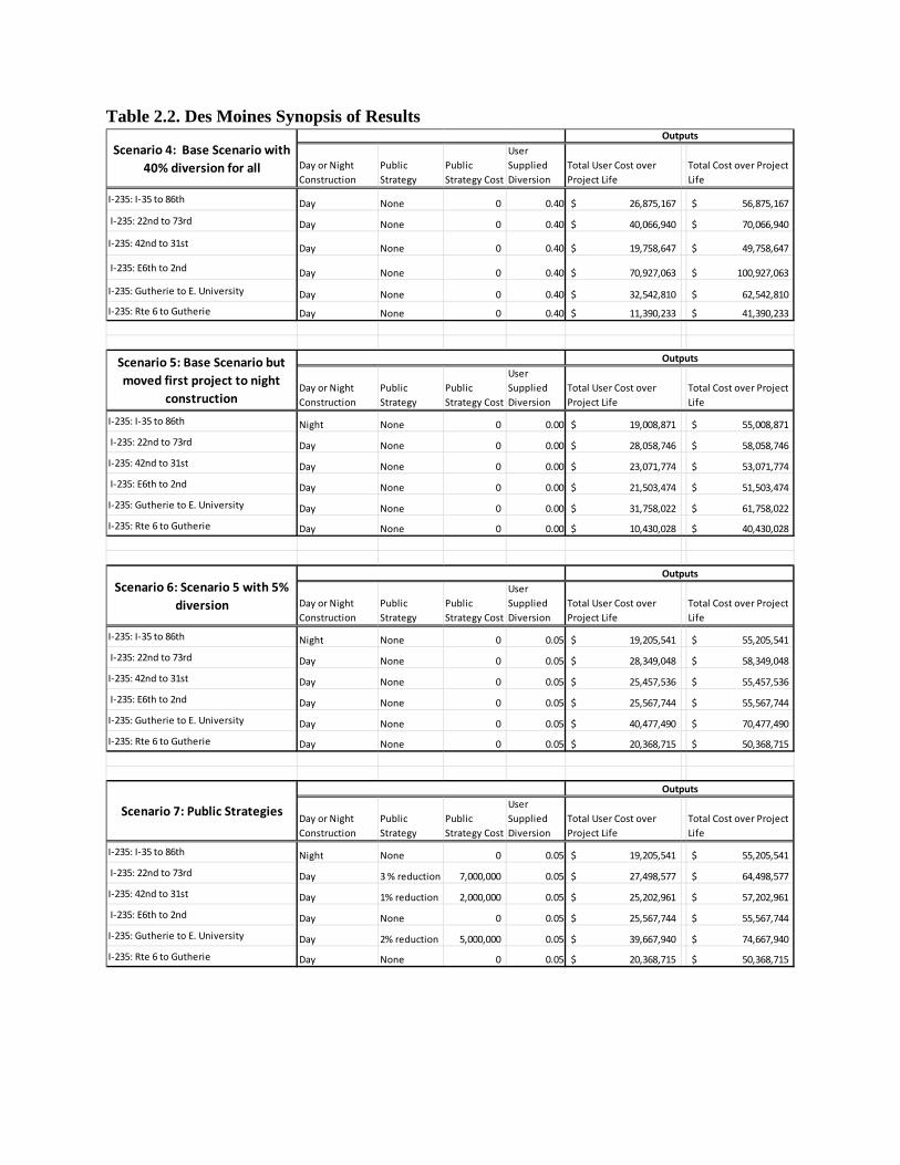
Table 2.2. Des Moines Synopsis of Results
Day or Night Construction
Public Strategy
Public Strategy Cost
User Supplied Diversion
Total User Cost over Project Life
Total Cost over Project Life
I-235: I-35 to 86th Day None 0 0.40 26,875,167$ 56,875,167$
I-235: 22nd to 73rd Day None 0 0.40 40,066,940$ 70,066,940$
I-235: 42nd to 31st Day None 0 0.40 19,758,647$ 49,758,647$
I-235: E6th to 2nd Day None 0 0.40 70,927,063$ 100,927,063$
I-235: Gutherie to E. University Day None 0 0.40 32,542,810$ 62,542,810$ I-235: Rte 6 to Gutherie Day None 0 0.40 11,390,233$ 41,390,233$
Day or Night Construction
Public Strategy
Public Strategy Cost
User Supplied Diversion
Total User Cost over Project Life
Total Cost over Project Life
I-235: I-35 to 86th Night None 0 0.00 19,008,871$ 55,008,871$
I-235: 22nd to 73rd Day None 0 0.00 28,058,746$ 58,058,746$
I-235: 42nd to 31st Day None 0 0.00 23,071,774$ 53,071,774$
I-235: E6th to 2nd Day None 0 0.00 21,503,474$ 51,503,474$
I-235: Gutherie to E. University Day None 0 0.00 31,758,022$ 61,758,022$
I-235: Rte 6 to Gutherie Day None 0 0.00 10,430,028$ 40,430,028$
Day or Night Construction
Public Strategy
Public Strategy Cost
User Supplied Diversion
Total User Cost over Project Life
Total Cost over Project Life
I-235: I-35 to 86th Night None 0 0.05 19,205,541$ 55,205,541$
I-235: 22nd to 73rd Day None 0 0.05 28,349,048$ 58,349,048$
I-235: 42nd to 31st Day None 0 0.05 25,457,536$ 55,457,536$
I-235: E6th to 2nd Day None 0 0.05 25,567,744$ 55,567,744$
I-235: Gutherie to E. University Day None 0 0.05 40,477,490$ 70,477,490$
I-235: Rte 6 to Gutherie Day None 0 0.05 20,368,715$ 50,368,715$
Day or Night Construction
Public Strategy
Public Strategy Cost
User Supplied Diversion
Total User Cost over Project Life
Total Cost over Project Life
I-235: I-35 to 86th Night None 0 0.05 19,205,541$ 55,205,541$
I-235: 22nd to 73rd Day 3 % reduction 7,000,000 0.05 27,498,577$ 64,498,577$
I-235: 42nd to 31st Day 1% reduction 2,000,000 0.05 25,202,961$ 57,202,961$
I-235: E6th to 2nd Day None 0 0.05 25,567,744$ 55,567,744$
I-235: Gutherie to E. University Day 2% reduction 5,000,000 0.05 39,667,940$ 74,667,940$
I-235: Rte 6 to Gutherie Day None 0 0.05 20,368,715$ 50,368,715$
Outputs
Outputs
Scenario 4: Base Scenario with 40% diversion for all
Scenario 5: Base Scenario but moved first project to night
construction
Scenario 6: Scenario 5 with 5% diversion
Scenario 7: Public Strategies
Outputs
Outputs

Table 2.3. Des Moines Synopsis of Results
Highlights: WISE outputs, in particular user costs and total project costs, appear to be
performing in the directions and approximate ranges expected as the inputs change.
• “Total User Cost over Project Life” declines with night construction (comparing Base Scenario with Scenario 5).
• With respect to diversion (Base Scenario and Scenarios 1 to 4), “Total User Cost over Project Life” has varied fairly systematically and predictably among the segments and across the diversion scenarios. Figures 2.3 and 2.4 demonstrate the user cost values arrayed by segment; Figure 2.5 user costs are arrayed by diversion percentage (Scenarios 1 through 4), and Figure 2.6 compares the user cost by strategy to the Base Scenario (Scenarios 5 through 8). All user cost values are displayed in millions of dollars.
Figure 2.3. Des Moines diversion (Div.) comparison scenarios by segment.
Day or Night Construction
Public Strategy
Public Strategy Cost
User Supplied Diversion
Total User Cost over Project Life
Total Cost over Project Life
I-235: I-35 to 86th Night None 0 0.05 19,205,541$ 55,205,541$
I-235: 22nd to 73rd Day None 0 0.05 21,261,786$ 54,261,786$
I-235: 42nd to 31st Day None 0 0.05 25,457,536$ 55,457,536$
I-235: E6th to 2nd Day None 0 0.05 25,567,744$ 55,567,744$
I-235: Gutherie to E. University Day None 0 0.05 40,477,490$ 70,477,490$
I-235: Rte 6 to Gutherie Day None 0 0.05 20,368,715$ 50,368,715$
Scenario 8: Scenario 6 + project 2 (bold) at 9 months and 10%
cost increase
Outputs
$- $10.0 $20.0 $30.0 $40.0 $50.0 $60.0 $70.0 $80.0
I-35 to 86th 22nd to 73rd 42nd to 31st E6th to 2nd Gutherie to E.University
Rte 6 to Gutherie
Mill
ions
DesMoines Diversion Comparison Scenarios By Segment
Base 1- Div. 5% 2- Div. 10% 3- Div. 20% 4- Div. 40%

Figure 2.4. Des Moines strategy comparison scenarios by segment.
Figure 2.5. Des Moines diversion comparison scenarios by diversion percentage.
$- $5
$10 $15 $20 $25 $30 $35 $40 $45
I-35 to 86th 22nd to 73rd 42nd to 31st E6th to 2nd Gutherie to E.University
Rte 6 toGutherie
Mill
ions
DesMoines Strategy Comparison Scenario By Segment
Base 5- Proj. 1 night 6- Scen. 5 5% div. 7- Public info. 8 - Scen 6 + Proj. 2 9 mos.
$-
$10
$20
$30
$40
$50
$60
$70
$80
Base 1- Div. 5% 2- Div. 10% 3- Div. 20% 4- Div. 40%
Mill
ions
DesMoines Diversion Comparison Scenarios By Diversion %
I-35 to 86th 22nd to 73rd 42nd to 31st E6th to 2nd Gutherie to E. University Rte 6 to Gutherie

Figure 2.6. Des Moines strategy comparison scenarios by strategy.
General WISE Calculation Engine Issues Throughout the Iowa testing, the main issue/observation with the WISE-supplied diversion relates to the WISE Diversion Calculation tool. Specifically,
• Diversion Calculator, which runs when “User Supplied Diversion” is set to 0, will always 100% divert traffic from the construction zone when an alternate link is available.
• Diversion Calculator results are inconsistent and unreliable, and in runs of the model the user-supplied diversion was based on the user’s experience. The microsimulation model can also be used to determine the percentage of diversion.
$- $5
$10 $15 $20 $25 $30 $35 $40 $45
Base 5- Proj. 1 night 6- Scen. 5 5% div. 7- Public info. 8 - Scen 6 + Proj.2 9 mos.
Mill
ions
DesMoines Strategy Comparison Scenarios By Strategy
I-35 to 86th 22nd to 73rd 42nd to 31st
E6th to 2nd Gutherie to E. University Rte 6 to Gutherie

CHAPTER 3 Phoenix, Arizona, Validation Test Deployment Introduction The Phoenix test case is the second of four WISE test subjects and the second of two validation test sites. It is also the first of two test sites where a separate microsimulation model test was performed to independently estimate diversion. A detailed description of the Phoenix project is included as Appendix A, Part 2. The Phoenix program of projects includes six projects as summarized below:
• Project A: 202L Red Mountain Freeway – 101L to Gilbert Road. 3-lane freeway, adding high occupancy vehicle (HOV) lane;
• Project B: 202L Santan Freeway – I-10 to Gilbert Road. 3-lane freeway, adding HOV lane and corresponding HOV directional ramps at I-10 and 101L;
• Project C: SR 101 HOV addition – SR 202 Red Mountain to Princess Drive; • Project D: Twin Peaks traffic interchange. – I-10 at MP 245. Traffic interchange addition
to I-10 at MP 245 for access to I-10 from Twin Peaks Road, approximately 13 miles northwest of downtown Tucson, in Marana;
• Project E: I-10 Kino Boulevard to Valencia Road; and • Project F: 202 Red Mountain Design Build – general purpose addition eastbound I-10 to
101, westbound 101 to Scottsdale Road.
Application of the WISE Program to the Phoenix Projects These six projects are associated with the east–west 202 corridor and the north–south 101 corridor. Both of these routes are freeways with limited access. Interchanges are closer than one mile in many areas. Each corridor is represented by dozens of key roadway segments. The 202 project corridor is approximately 14 miles long, and the 101 corridor is approximately 15 miles long.
As noted in the Iowa test case, the WISE program was developed using a test network that was the highway network for the island of Guam. The Guam test network is simple when compared to these two heavily traveled corridors. Summary of Testing Procedures and Scenarios The configuration of the Route 202 and 101 corridors and the construction phasing presented problems for the WISE software, since WISE considers a single construction project as occurring on a single highway segment. The software does not have the ability to consider that a construction project might involve numerous roadway segments. Consequently, the WISE test could not fully evaluate the construction projects as defined. Instead, the test case was developed by selecting four key roadway segments in each of the two corridors (eight project sites). WISE

was used to determine a scheduling sequence and estimate the user costs associated with the construction activities. The eight test sites were as follows:
1. Route 101 Pima Freeway ( FWY), north of Loop 202 Red Mountain FWY (subset of Project C, above)
2. Route 101 Pima FWY, north of E. McDowell Road (subset Project C) 3. Route 101 Pima FWY, north of E. Indian School Road (subset Project C) 4. Route 101 Pima FWY, north of E. Desert Cove Drive (subset Project C) 5. Route 202 Red Mountain FWY, west of Route 101(subset Project A) 6. Route 202 Red Mountain FWY, west of N Scottsdale Road (subset Project A) 7. Route 202 Red Mountain FWY, west of N Priest Drive (subset Project A) 8. Route 202 Red Mountain FWY, E. Van Buren Street (subset Project A)
WISE Data Preparation WISE requires a coded network as input, along with a TAZ file. These inputs were acquired from the Maricopa Association of Governments. The material supplied by Maricopa included a TransCAD-based regional travel demand forecasting model, complete with TAZs and travel model estimated traffic volumes. With this model as a base, the following steps were then followed to create the needed WISE inputs:
1. A windowed highway network of Phoenix was extracted following the Route 202 and Route 101 corridors.
2. Following a similar selection process, the TAZ polygons were extracted from the model for the same area as the highway network.
3. WISE requires that all network nodes must be within a TAZ polygon. Consequently, the highway network was further trimmed so all nodes were within the boundaries set by the extracted TAZs.
4. Because of the extraction of TAZs, the TAZ centroids and their connectors to the highway network had to be redefined to make sense for this much smaller area.
5. WISE does not accept one-way roads. This presented a technical hurdle because the entire roadway system from the Maricopa model is coded using one-way pairs, particularly on freeways and ramps. The two-way coding accurately reflected the directional attributes associated with the one-way pairs. In addition to the freeways, all the ramps had to be converted to intersections.
6. The WISE program was having difficulty accepting the files from TransCAD. Consequently, to streamline the inputs, all the node numbers in the model were renumbered sequentially beginning with 1. Centroids were renumbered as the first sequence, and network nodes followed (although a small numbering gap was used to separate centroids from network nodes). This renumbering was performed in TransCAD by using the interactive tools.

7. A required input of WISE is a file of node numbers and the TAZ within which the node resides. This “tagging” of the nodes with the TAZ ID was performed interactively with TransCAD.
8. Finally, a TransCAD GISDK script was written to build all the needed input files directly from the coded TransCAD network. This GISDK script was written as a batch macro, a copy of which is included as Appendix C, Part 2.
Figure 3.1 below shows a rendering of the coded highway network. Figure 3.2 shows a
blowup of the Route 101 and Route 202 interchange area.
Figure 3.1 Phoenix code network.

Figure 3.2 Route 202/101 interchange blowup.
Scenario Summaries Testing was performed simultaneously for the two corridors with four projects in each corridor. The Phoenix validation also included the test of the importance of the Operation Module. The Operation Module employs microsimulation models and networks to provide more sophisticated estimates of diversion that can be fed back into the WISE Planning Module for a more robust analysis. WISE was developed to work with the nonproprietary DynusT network microsimulation models. However, any reasonably robust microsimulation model will provide diversion estimates for work zone projects; in this case TransModeler was used to develop the diversion estimates for a sixth scenario. The diversion estimates were fed back into the WISE Planning Module to compare the differences in results between user-supplied diversion and microsimulation modeled diversion. Five schedule scenarios (six including the base scenario) were tested with WISE as follows:
1. Base Scenario—All projects feed into WISE with daytime construction and without any mitigation strategies.
2. Scenario 1—Base Scenario with Project 1 required to start after Project 8 and diversion set to 5% for all eight projects.
3. Scenario 2—Scenario 1 with travel diversion set to 10% for all eight projects. 4. Scenario 3—Scenario 1 with travel diversion set to 15% for all eight projects.

5. Scenario 4 —Scenario 1 with travel diversion set to 15% and Project 8 set with a demand strategy.
6. Scenario 5—Diversion developed in TransModeler. Travel diversion estimated in separate microsimulation model runs and manually fed back into the WISE model for comparison purposes (to test the difference made from using Operation Module components).
Synopsis of Validation Results Because of the linear nature of both the Route 101 and Route 202 corridors, WISE had difficulty in generating schedule changes (although it did generate differences in user costs). Basically, along linear corridors, there is little interaction between the corridors, and therefore, little justification for making changes other than to simply let all corridor construction run concurrently. This makes some sense given the large separation (upwards of 20 miles) between some of the project segments. Summary Results A summary of the results has been documented in the spreadsheet <Validation_Results.xlsx>, tab <AZ Results> (which is included as a separate file). Table 3.1 summarizes the key inputs and findings on user cost. The original Excel version of this table and the graphs are included in the spreadsheet <Validation_Results.xlsx>, tab <AZ Synopsis and Graphics>.

Table 3.1. Synopsis of Phoenix Validation
Public Strategy
Public Strategy Cost
User Supplied Diversion
Total User Cost over Project Life
Rte 101 - PIMA FWY, n/o Loop 202 Red Mountain FWY None 0 0.00 25,381,286$ Rte 101 - PIMA FWY, n/o E McDowell Rd None 0 0.00 9,964,797$ Rte 101 - PIMA FWY, n/o E Indian School Rd None 0 0.00 16,070,102$ Rte 101 - PIMA FWY, n/o E Desert Cove Dr None 0 0.00 28,755,213$ Rte 202 - Red Mountain FWY, w/o Rte 101 None 0 0.00 17,293,915$ Rte 202 - Red Mountain FWY, w/o N Scottsdale Rd None 0 0.00 31,940,198$ Rte 202 - Red Mountain FWY, w/o N Priest Dr None 0 0.00 31,940,198$ Rte 202 - Red Mountain FWY, w/o E Van Buren St None 0 0.00 26,456,423$
Public Strategy
Public Strategy Cost
User Supplied Diversion
Total User Cost over Project Life
Rte 101 - PIMA FWY, n/o Loop 202 Red Mountain FWY None 0 0.05 25,381,286$ Rte 101 - PIMA FWY, n/o E McDowell Rd None 0 0.05 9,964,797$ Rte 101 - PIMA FWY, n/o E Indian School Rd None 0 0.05 16,070,102$ Rte 101 - PIMA FWY, n/o E Desert Cove Dr None 0 0.05 27,151,747$ Rte 202 - Red Mountain FWY, w/o Rte 101 None 0 0.05 17,293,915$ Rte 202 - Red Mountain FWY, w/o N Scottsdale Rd None 0 0.05 27,151,747$ Rte 202 - Red Mountain FWY, w/o N Priest Dr None 0 0.05 27,151,747$ Rte 202 - Red Mountain FWY, w/o E Van Buren St None 0 0.05 27,151,747$
Public Strategy
Public Strategy Cost
User Supplied Diversion
Total User Cost over Project Life
Rte 101 - PIMA FWY, n/o Loop 202 Red Mountain FWY None 0 0.10 36,634,150$ Rte 101 - PIMA FWY, n/o E McDowell Rd None 0 0.10 14,221,885$ Rte 101 - PIMA FWY, n/o E Indian School Rd None 0 0.10 21,204,175$ Rte 101 - PIMA FWY, n/o E Desert Cove Dr None 0 0.10 33,884,627$ Rte 202 - Red Mountain FWY, w/o Rte 101 None 0 0.10 24,937,936$ Rte 202 - Red Mountain FWY, w/o N Scottsdale Rd None 0 0.10 39,008,950$ Rte 202 - Red Mountain FWY, w/o N Priest Dr None 0 0.10 39,008,950$ Rte 202 - Red Mountain FWY, w/o E Van Buren St None 0 0.10 39,008,950$
Public Strategy
Public Strategy Cost
User Supplied Diversion
Total User Cost over Project Life
Rte 101 - PIMA FWY, n/o Loop 202 Red Mountain FWY None 0 0.15 48,028,333$ Rte 101 - PIMA FWY, n/o E McDowell Rd None 0 0.15 18,686,145$ Rte 101 - PIMA FWY, n/o E Indian School Rd None 0 0.15 27,132,013$ Rte 101 - PIMA FWY, n/o E Desert Cove Dr None 0 0.15 40,863,071$ Rte 202 - Red Mountain FWY, w/o Rte 101 None 0 0.15 32,619,692$ Rte 202 - Red Mountain FWY, w/o N Scottsdale Rd None 0 0.15 51,053,023$ Rte 202 - Red Mountain FWY, w/o N Priest Dr None 0 0.15 51,053,023$ Rte 202 - Red Mountain FWY, w/o E Van Buren St None 0 0.15 51,053,023$
Base Scenario
Inputs Outputs
Scenario 1: All Diversions set to 5% (with Project 1 required to start after Project 8 - for
all other scenarios as well)
Inputs Outputs
Scenario 2: All Diversions set to 10%
Inputs Outputs
Scenario 3: All Diversions set to 15%
Inputs Outputs
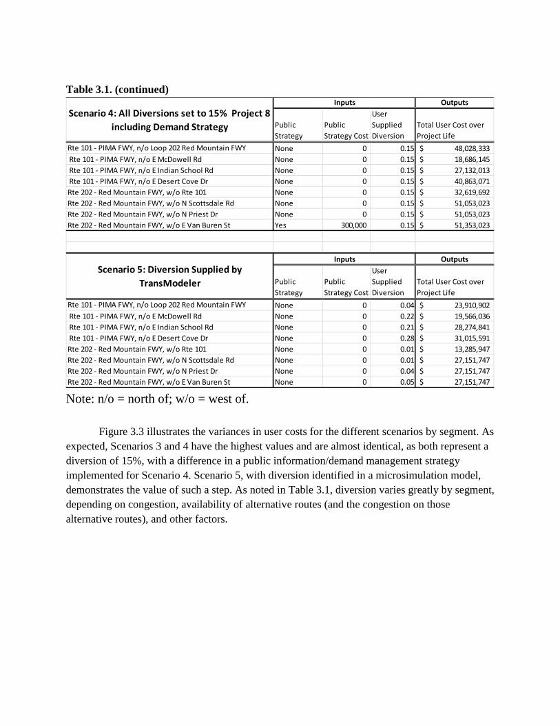
Table 3.1. (continued)
Note: n/o = north of; w/o = west of.
Figure 3.3 illustrates the variances in user costs for the different scenarios by segment. As expected, Scenarios 3 and 4 have the highest values and are almost identical, as both represent a diversion of 15%, with a difference in a public information/demand management strategy implemented for Scenario 4. Scenario 5, with diversion identified in a microsimulation model, demonstrates the value of such a step. As noted in Table 3.1, diversion varies greatly by segment, depending on congestion, availability of alternative routes (and the congestion on those alternative routes), and other factors.
Public Strategy
Public Strategy Cost
User Supplied Diversion
Total User Cost over Project Life
Rte 101 - PIMA FWY, n/o Loop 202 Red Mountain FWY None 0 0.15 48,028,333$ Rte 101 - PIMA FWY, n/o E McDowell Rd None 0 0.15 18,686,145$ Rte 101 - PIMA FWY, n/o E Indian School Rd None 0 0.15 27,132,013$ Rte 101 - PIMA FWY, n/o E Desert Cove Dr None 0 0.15 40,863,071$ Rte 202 - Red Mountain FWY, w/o Rte 101 None 0 0.15 32,619,692$ Rte 202 - Red Mountain FWY, w/o N Scottsdale Rd None 0 0.15 51,053,023$ Rte 202 - Red Mountain FWY, w/o N Priest Dr None 0 0.15 51,053,023$ Rte 202 - Red Mountain FWY, w/o E Van Buren St Yes 300,000 0.15 51,353,023$
Public Strategy
Public Strategy Cost
User Supplied Diversion
Total User Cost over Project Life
Rte 101 - PIMA FWY, n/o Loop 202 Red Mountain FWY None 0 0.04 23,910,902$ Rte 101 - PIMA FWY, n/o E McDowell Rd None 0 0.22 19,566,036$ Rte 101 - PIMA FWY, n/o E Indian School Rd None 0 0.21 28,274,841$ Rte 101 - PIMA FWY, n/o E Desert Cove Dr None 0 0.28 31,015,591$ Rte 202 - Red Mountain FWY, w/o Rte 101 None 0 0.01 13,285,947$ Rte 202 - Red Mountain FWY, w/o N Scottsdale Rd None 0 0.01 27,151,747$ Rte 202 - Red Mountain FWY, w/o N Priest Dr None 0 0.04 27,151,747$ Rte 202 - Red Mountain FWY, w/o E Van Buren St None 0 0.05 27,151,747$
Scenario 4: All Diversions set to 15% Project 8 including Demand Strategy
Inputs Outputs
Scenario 5: Diversion Supplied by TransModeler
Inputs Outputs

Figure 3.3 Phoenix user cost comparison scenarios by segment.
Figure 3.4 compares user cost across the different segments by diversion percentage.
Figure 3.4. Phoenix user cost comparison scenarios by diversion percentage.
Computer Running Time and Requirements
$-
$10.0
$20.0
$30.0
$40.0
$50.0
$60.0
Rte 101 n/o L202 RM Fwy
Rte 101 n/o EMcD+R8 Rd
Rte 101 n/o EI S Rd
Rte 101 n/o ED C Dr
Rte 202 w/oRte 101
Rte 202 w/o NS Rd
Rte 202 w/o NP Dr
Rte 202 w/o EV B St
Mill
ions
Phoenix User Cost Comparison Scenarios- By Segment
Base 1: Div.5% 2: Div. 10% 3: Div. 15% 4: Div.15% + PI 5: Ops.Model Div.
$-
$10
$20
$30
$40
$50
$60
Base 1: Div.5% 2: Div. 10% 3: Div. 15% 4: Div.15% + PI 5: Ops.Model Div.
Mill
ions
Phoenix User Cost Comparison Scenarios - By Diversion %
Rte 101 n/o L 202 RM Fwy Rte 101 n/o E McD+R8 Rd Rte 101 n/o E I S Rd Rte 101 n/o E D C Dr
Rte 202 w/o Rte 101 Rte 202 w/o N S Rd Rte 202 w/o N P Dr Rte 202 w/o E V B St
The final coded network that was input to WISE had 779 roadway segments and 725 nodes (inclusive of centroid connectors). The coding of this network (following the steps referenced above) took approximately 85 person-hours. Once the network was completed, another 20 hours were spent running the WISE conversion program and making additional network edits to address errors reported by WISE.
Once the network was in WISE, the additional coding of work zones only took a few minutes. The testing of each construction program (for this test, eight work zones were included in each construction program) took approximately 2 hours. Of the 2-hour time frame, WISE took 1 hour and 50 minutes to test a work program. The remainder of the time was spent working through the interactive user’s interface and analyzing the results. WISE is a 32-bit program, but these WISE runtimes reflect WISE’s performance on a 64-bit workstation, with 12 CPUs, and solid state drives. On a more modest 64-bit laptop, with mechanical drives, the runtime would be three to four times longer. Software Modifications and Graphical User Interface Update During the first test site application (Iowa), there were a considerable number of edits to WISE. However, no additional edits were made to WISE during this second test site application.

CHAPTER 4 Wise Pilot Test Deployment: Orlando, Florida Introduction The Orlando test case is the third of four WISE test subjects and the first of the two pilot tests. It is also the second site (in addition to Phoenix) where operational microsimulation model testing was applied to more accurately estimate diversion and to compare the results with user-supplied diversion. A detailed description of the Orlando project is included as Appendix B. Generally, the Orlando project is the reconstruction of I-4, SR 400 in Orange and Seminole Counties to accommodate three general use lanes, auxiliary lanes, and two managed lanes in the eastbound and westbound directions. The project corridor is approximately 20 miles long.
Summary of Testing Procedures and Scenarios Application of the WISE Program to the Orlando Projects As discussed in Chapters 2 and 3, the WISE program was developed by using a test network that was the highway network for the island of Guam. This test network is simple when compared to the Orlando network.
The configuration of I-4 construction phasing presented problems for the WISE software, because WISE considers a single construction project as occurring on a single highway segment. The software does not have the ability to consider that a construction project might involve numerous roadway segments. The Orlando I-4 project includes the reconstruction of 14 interchanges and the modification of five other bridges.
One of the challenges of this test site application was to configure a WISE example that fits within WISE’s constraints and that could be useful for evaluating the I-4 corridor. That test case was developed by selecting four key roadway segments in the project corridor. These test segments are as follows:
1. I-4, north of State Highway 436 2. I-4, north of Lee Road 3. I-4, north of Ivanhoe Boulevard 4. I-4, north of State Highway 50
WISE Data Preparation WISE requires a coded network as input, along with a TAZ file. These inputs were acquired from the TransModeler microsimulator for the Orlando area calibrated to counts downloaded from STEWARD. With this model as a base, the following steps were then followed to create the needed WISE inputs:

1. A windowed highway network of Orlando was extracted to more narrowly define the I-4 corridor.
2. WISE requires that all network nodes must be within a TAZ polygon. TAZ polygons did not exist for the I-4 model, although centroids (sinks and sources) were defined. With the use of the defined centroids a polygon layer was created to represent the zone boundaries.
3. WISE does not accept one-way roads. This presented a technical hurdle because the entire roadway system is coded by using one-way pairs particularly on freeways and ramps. This recoding had to properly reflect the directional attributes of the one-way pairs in the two-way coding. In addition to the Interstate, all the ramps/interchanges had to be converted to intersections.
4. Consistent with the steps followed for Des Moines and Phoenix, all the node numbers in the model were renumbered sequentially beginning with 1, to facilitate importing the network into WISE. Centroids were renumbered as the first sequence, and network nodes followed (although a small numbering gap was used to separate centroids from network nodes). This renumbering was performed in TransModeler using the interactive tools.
5. A required input to WISE is a file of node numbers and the TAZ within which the node resides. This “tagging” of the nodes with the TAZ ID was performed interactively with TransModeler.
6. Next the TransModeler files were output to TransCAD, which is a sister program to TransModeler.
7. Finally, a TransCAD GISDK script was written to build all the needed input files directly from the coded TransCAD network. This GISDK script was written as a batch macro, a copy of which is included as Appendix C, Part 3.
Figure 4.1 below shows a rendering of the coded highway network.

Figure 4.1. Orlando code network.

Synopsis of Pilot Test Results Summary Results Testing Summary results testing was performed for five conditions: the Base Scenario and test Scenarios 1, 2, 3, and 4. The five scenarios and the results of the testing are discussed below. As a point of reference, Project 1 is at the northernmost point of the analysis corridor; Project 4 is at the southern end, and Projects 2 and 3 are middle sections from north to south respectively. The details of the WISE output are summarized in the Excel worksheet labeled <Pilot_Results.xlsx>, tab <Orlando Results>.
1. Scenario Base Case. The initial condition given to WISE was for each of the four project segments to have a cost of $30 million with an earliest start date of May 1, 2012. Each project was given a daytime construction period without any mitigation strategies. For this scenario, WISE output had the most northern project segment (I-4, north of State Highway 436) starting at the beginning of the construction program. Similarly, the third segment (I-4, north of Ivanhoe Boulevard, which is in the middle of the analysis corridor) also started at the beginning of the program. Project 2 and Project 4 were scheduled to begin after the completion of Projects 1 and 3. Consequently, Projects 2 and 4 were scheduled to start in February of 2013.
2. Scenario 1, Base Scenario with Project 1 and Project 3 having a 5% user-defined diversion. After running this scenario, there was no change to the construction sequencing selected by WISE. However, the diversion did not produce a reduction in user costs. Instead, user costs were higher. This increase is due to the lack of alternate routes in the coded highway network. Thus alternate routes are much longer and just as congested as the prime route I-4.
3. Scenario 2, Base Scenario with Project 1 and Project 3 having a 5% user-defined diversion and 2% demand reductions for a radius of 5 miles. This did result in generally a 2% reduction in user costs reflecting the lower demand, and this scenario consisted of a $2 million agency implementation cost, which is reflected in the total project cost.
4. Scenario 3, Base Scenario with Project 1 and Project 3 having night construction. For this scenario, it was assumed that night construction resulted in a 50% increase in construction cost. This is reflected in the WISE output, which shows the higher agency cost. However, the nighttime traffic volumes are much lower than the daytime volumes, which accounts for the significant drop in user costs.
5. Scenario 4, Base Scenario with diversion calculated by TransModeler. Employing the microsimulation model verified the observation that very little diversion would be expected due to the lack of alternate routes. The microsimulation estimated a 4% diversion for the third project.

Table 4.1 summarizes some key inputs and outputs of the WISE model. Total project costs are displayed in addition to user costs because of the shifts between agency costs and user costs developed in Scenario 3 with night construction.
Table 4.1. Orlando Synopsis of Results
Figure 4.2 graphically illustrates the changes (and lack of changes, in some cases) in user
costs for the different scenarios and segments. Project 3 demonstrates the spike in user cost when diversion is forced with no viable alternate routes (second and third bars compared with the base case.) Projects 1 and 3 demonstrate the dramatic drop in user costs when night construction is undertaken (fourth bars). Projects 2 and 4 demonstrate the consistency of the user costs when no
Day or Night Construction Public Strategy
User Supplied Diversion
Total User Cost over Project Life
Total Cost over Project Life
Interstate 4, n/o State Highway 436 Day None 0.00 95,593,464$ 125,593,464$ Interstate 4, n/o Lee Road Day None 0.00 58,347,704$ 88,347,704$ Interstate 4, n/o Ivanhoe Boulevard Day None 0.00 83,940,784$ 113,940,784$ Interstate 4, n/o State Highway 50 Day None 0.00 39,749,537$ 69,749,537$
Day or Night Construction Public Strategy
User Supplied Diversion
Total User Cost over Project Life
Total Cost over Project Life
Interstate 4, n/o State Highway 436 Day None 0.05 97,983,302$ 127,983,302$ Interstate 4, n/o Lee Road Day None 0.00 58,347,704$ 88,347,704$ Interstate 4, n/o Ivanhoe Boulevard Day None 0.05 147,133,553$ 177,133,553$ Interstate 4, n/o State Highway 50 Day None 0.00 39,749,537$ 69,749,537$
Day or Night Construction Public Strategy
User Supplied Diversion
Total User Cost over Project Life
Total Cost over Project Life
Interstate 4, n/o State Highway 436 Day2% demand reduction, 5 mile radius, $2 million 0.05 96,023,635$ 128,023,635$
Interstate 4, n/o Lee Road Day None 0.00 58,347,704$ 88,347,704$
Interstate 4, n/o Ivanhoe BoulevardDay
2% demand reduction, 5 mile radius, $2 million 0.05 144,190,881$ 176,190,881$
Interstate 4, n/o State Highway 50 Day None 0.00 39,749,537$ 69,749,537$
Day or Night Construction Public Strategy
User Supplied Diversion
Total User Cost over Project Life
Total Cost over Project Life
Interstate 4, n/o State Highway 436 Night None 0.00 29,633,974$ 74,633,974$ Interstate 4, n/o Lee Road Day None 0.00 58,347,704$ 88,347,704$ Interstate 4, n/o Ivanhoe Boulevard Night None 0.00 26,021,643$ 71,021,643$ Interstate 4, n/o State Highway 50 Day None 0.00 39,749,537$ 69,749,537$
Day or Night Construction Public Strategy
User Supplied Diversion
Total User Cost over Project Life
Total Cost over Project Life
Interstate 4, n/o State Highway 436 Day None 0.00 95,593,464$ 125,593,464$ Interstate 4, n/o Lee Road Day None 0.00 58,347,704$ 88,347,704$ Interstate 4, n/o Ivanhoe Boulevard Day None 0.04 146,869,469$ 176,869,469$ Interstate 4, n/o State Highway 50 Day None 0.00 39,749,537$ 69,749,537$
Outputs
Outputs
Outputs
Outputs
Outputs
InputsScenario 4: TransModeler Supplied
Diversion
Inputs
Inputs
Scenario 2: Base Scenario with Project 1 and Project 3 having a 5% Diversion
and 2% reduction in demand
Scenario 3: Base Scenario with Project 1 and Project 3 having night
construction
Inputs
Inputs
Base Scenario
Scenario 1: Base Scenario with Project 1 and Project 3 having a 5% diversion

viable alternate routes are available, without the intervention of strategies such as night construction.
Figure 4.2 Orlando user cost comparison by segment.
Figure 4.3 compares the user cost by strategy or diversion percentage. Again, the most
dramatic case is the significant change in user cost when nighttime construction is employed. “Forced” diversion in Scenarios 1 and 2, and in the microsimulation estimate in Scenario 4, increases user costs when no viable alternatives are available.
Figure 4.3 Orlando user cost by diversion percentage or strategy.
$-
$20.0
$40.0
$60.0
$80.0
$100.0
$120.0
$140.0
$160.0
Interstate 4, n/o State Highway 436 Interstate 4, n/o Lee Road Interstate 4, n/o Ivanhoe Boulevard Interstate 4, n/o State Highway 50
Mill
ions
Orlando User Cost Comparison By Segment
Base 1- Div. 5% 2- Div. 5% , Red. 2% 3- Night Con. 4- Ops.Model Div.
$-
$20.0
$40.0
$60.0
$80.0
$100.0
$120.0
$140.0
$160.0
Base 1- Div. 5% 2- Div. 5% , Red. 2% 3- Night Con. 4- Ops.Model Div.
Mill
ions
Orlando User Cost Comparison By Diversion %
Interstate 4, n/o State Highway 436 Interstate 4, n/o Lee Road Interstate 4, n/o Ivanhoe Boulevard Interstate 4, n/o State Highway 50

Computer Running Time and Requirements The final coded network, which was input to WISE, had 304 roadway segments and 240 nodes (inclusive of centroid connectors). The coding of this network (following the steps referenced above) took approximately 27 person-hours. Once the network was completed, another 3 hours was spent running the WISE conversion program and making additional network edits to address errors reported by WISE.
Once the network was in WISE, the additional coding of work zones only took a few minutes. The testing of each construction program (for this test, four work zones were included in each construction program) took approximately 4 minutes.
WISE is a 32-bit program, but these WISE runtimes reflect WISE’s performance on a 64-bit workstation, with 12 CPUs, and solid state drives. On a more modest 64-bit laptop, with mechanical drives, the runtime would be three to four times longer. Software Modifications and Graphical User Interface Update During the first test site application (Iowa), there were a considerable number of edits to WISE. However, no additional edits were made to WISE during this third test site application.

CHAPTER 5 Pilot Test Deployment: Worcester, Massachusetts Introduction The Worcester, test case is the second pilot test and the fourth of four WISE test subjects. The Worcester project is the reconstruction of four areas along the Route 9 corridor as follows:
1. The first location (and easternmost project location) is the replacement of the Route 9 bridge over Lake Quinsigamond. The Lake Quinsigamond bridge supports two travel lanes in each direction and has an average weekday travel (AWDT) over 52,000. There is an at-grade intersection at either end of the bridge. The next crossing of Lake Quinsigamond to the north is I-290, and this crossing is over 1.4 miles north. The next crossing to the south is Route 20, which is 2.6 miles south. Consequently, Route 9 is a major crossing point, and alternate routes would require considerable travel diversion.
2. The second construction project is the redecking of the Route 9/Belmont Street bridge over I-290. This construction project is close to the Worcester central business district (CBD). This bridge is two lanes in each direction and has an AWDT of 40,000. I-290 forms a partial diamond interchange at this location, so there is a considerable number of turning movements in this area.
3. The third project is an intersection improvement project equidistant between the first and second projects.
4. The fourth project is also an intersection improvement project 0.50 mile west of Project 2.
Summary of Testing Procedures Application of the WISE Program to the Worcester Projects To aid in the creation of a network for WISE, the regional TransCAD model maintained by the Worcester MPO and its staff, the Central Massachusetts Regional Planning Commission (CMRPC) was used. The CMRPC model is a TransCAD-based model calibrated to 2010 travel conditions. The CMRPC model served as a good candidate for the testing of WISE, since the previous three test sites were TransCAD/TransModeler models. This means that software developed to reformat a TransCAD model for WISE input had already been prepared.
The WISE program has some data limitations that need consideration when preparing a network. A major consideration is the inability of WISE to accept roads that are one-way. All roads input to WISE must be two-way.
For the analysis of the Worcester projects, the network should include I-290 through Worcester, since this facility has an interchange with one of the project sites, Belmont Street. Also, I-290 is one of the alternate routes to the Route 9 bridge replacement over Lake

Quinsigamond. Consequently, I-290 was needed in the WISE network, and this meant that the facility had to be coded as two-way with intersections instead of interchanges.
Another area within the Worcester study corridor with one-way roads is the Route 9 corridor itself. Route 9 as represented in the regional travel demand forecasting model is mostly coded as one-way pairs since large lengths of Route 9 have a median. Also, Worcester (like many major cities in New England) is comprised of mostly one-way street pairs in the CBD. Since the WISE study area passes across the northern end of the CBD, this meant that many roads had to be re-represented as two-way roads.
Finally, one of Worcester’s major traffic circles (Washington Square) is within the study area. This traffic circle had to be recoded as an intersection. WISE Data Preparation WISE requires a coded network as input, along with a TAZ file. These inputs were acquired from the TransCAD model supplied by CMRPC. With this model as a base, the following steps were taken to create the needed WISE inputs:
1. A windowed highway network of the Route 9 corridor was extracted from the Worcester model.
2. WISE requires that all network nodes must be within a TAZ polygon. Consequently the TAZ polygons from the CMRPC model were also windowed to the same area.
3. As referenced above, the one-way roads had to be re-represented as two-way. This resulted in recoding of all the one-way roads and the creation of intersections instead of interchanges. To perform this conversion, the congested highway times and volumes from the opposite direction had to be brought over to a common two-way link.
4. Following the network recoding, the network nodes were renumbered such that the centroid zones were given numbers starting at 1, and network nodes were given numbers starting at a number sequence slightly larger than the centroids. This renumbering also meant that the TAZs were also renumbered to match the new centroid numbers.
5. Using TransCAD’s “tagging” feature, network nodes were then tagged with the ID of the TAZ where the nodes reside.
6. Finally, a TransCAD GISDK script was written to build all the needed WISE input files directly from the coded TransCAD network. This GISDK script was written as a batch macro, a copy of which is included as Appendix C, Part 4.
In summary, the WISE representation of the Worcester model had 532 nodes, 716 links, and
112 zones. Figure 5.1 below shows a rendering of the coded highway network. Figure 5.2 shows a
blowup of the northern end of the Worcester CBD with Route 9.

Figure 5.1. Worcester code network.

Figure 5.2. Worcester area blowup.
Synopsis of Scenarios and Pilot Test Results The testing consisted of five scenarios as shown below. The detailed results are in the Excel spreadsheet labeled <Pilot_Results.xlsx>, tab <WorcesterResults>.
1. Base Scenario—The initial scenario given to WISE was to simply provide the project costs and duration. WISE used the input information to determine the initial construction sequencing. That sequencing is to have Projects 2, 3, and 4 all start in the first month of construction, and Project 1, the largest project, would start the following year.
2. Scenario 1—Base Scenario with Project 2 and Project 4 constructed at night. Only these two projects are candidates for nighttime construction because the traffic management plans for Projects 1 and 3 are so extensive that they must remain set up throughout the entire construction period. Shifting Projects 2 and 4 to nighttime construction did not change the construction sequencing, but the user costs are significantly lower, so low in fact that they outweigh the increased agency costs.
3. Scenario 2—Base Scenario with a public strategy to reduce travel by 5%. These demand reduction strategies were applied to all four projects. WISE did not compute any change in project scheduling due to this strategy. A 5% reduction seemed attainable with signage to divert traffic away from the corridor.

4. Scenario 3—Base Scenario with a public strategy to reduce travel by 10%. The demand reduction did not change the WISE schedule. WISE seems to appropriately compute the reduced user costs although WISE did not fully take into account the cost of travel on the diversion routes.
5. Scenario 4—Base Scenario with a public strategy to reduce travel by 15%. This seems like the greatest possible diversion that could be achieved. Since there are two major hospitals in the corridor, there is a possibility that off-site employee parking could be consolidated and travel through the corridor associated with hospital employees and shuttles could be reduced. However, as with the other demand reduction strategies, WISE did not change the construction sequencing. WISE did, however, appropriately show changes in user costs, although the user costs associated with operating on diversion routes is not fully quantified.
Synopsis of Results Table 5.1 summarizes the scenarios and the results of the analysis. User costs and total cost including agency cost are shown, to illustrate the relative impact of night construction on user cost and agency cost.
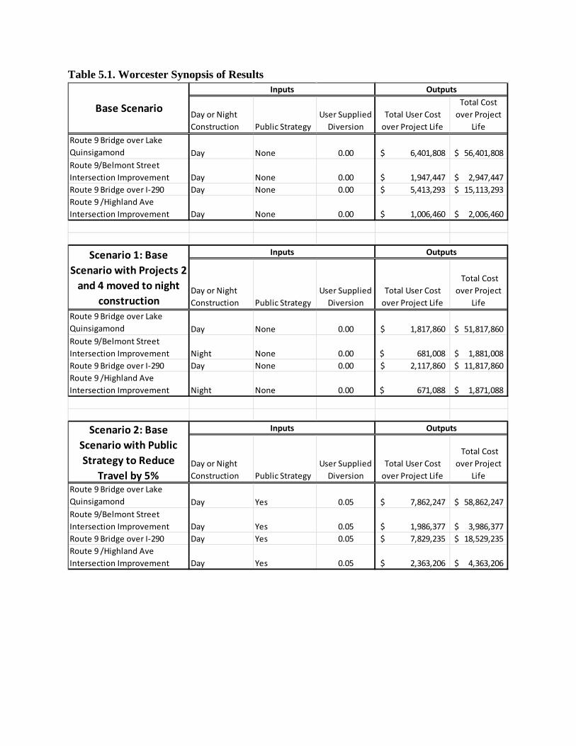
Table 5.1. Worcester Synopsis of Results
Day or Night Construction Public Strategy
User Supplied Diversion
Total User Cost over Project Life
Total Cost over Project
LifeRoute 9 Bridge over Lake Quinsigamond Day None 0.00 6,401,808$ 56,401,808$ Route 9/Belmont Street Intersection Improvement Day None 0.00 1,947,447$ 2,947,447$ Route 9 Bridge over I-290 Day None 0.00 5,413,293$ 15,113,293$ Route 9 /Highland Ave Intersection Improvement Day None 0.00 1,006,460$ 2,006,460$
Day or Night Construction Public Strategy
User Supplied Diversion
Total User Cost over Project Life
Total Cost over Project
Life Route 9 Bridge over Lake Quinsigamond Day None 0.00 1,817,860$ 51,817,860$ Route 9/Belmont Street Intersection Improvement Night None 0.00 681,008$ 1,881,008$ Route 9 Bridge over I-290 Day None 0.00 2,117,860$ 11,817,860$ Route 9 /Highland Ave Intersection Improvement Night None 0.00 671,088$ 1,871,088$
Day or Night Construction Public Strategy
User Supplied Diversion
Total User Cost over Project Life
Total Cost over Project
Life Route 9 Bridge over Lake Quinsigamond Day Yes 0.05 7,862,247$ 58,862,247$ Route 9/Belmont Street Intersection Improvement Day Yes 0.05 1,986,377$ 3,986,377$ Route 9 Bridge over I-290 Day Yes 0.05 7,829,235$ 18,529,235$ Route 9 /Highland Ave Intersection Improvement Day Yes 0.05 2,363,206$ 4,363,206$
Outputs
Outputs
Outputs
Base Scenario
Inputs
Scenario 1: Base Scenario with Projects 2
and 4 moved to night construction
Inputs
Scenario 2: Base Scenario with Public Strategy to Reduce
Travel by 5%
Inputs

Table 5.1. Worcester Synopsis of Results (continued)
Figure 5.3 demonstrates the different effects that the same strategy can have on user costs
in different segments. Note how the increase in diversion through public strategies (Columns 3, 4, and 5 in each segment) initially increases user costs over the base case, but then steadily decreases user costs in the first, third, and fourth project segments, while leading to an increase in user costs in the second project segment. This suggests that WISE is sensitive to differences in accessibility and congestion in different project segments, which is a positive attribute. The second bar from the left in each project segment (Scenario 1) illustrates the dramatic reduction in user costs (in this case for all projects, constructed day or night) that can be accomplished through night construction strategies.
This finding was unusual enough to demand further examination. Briefly, the night construction strategy for the Belmont project in particular opens up the corridor and allows more daytime diversion from the Lake Quinsigamond bridge to move north, thus decreasing user costs for the entire corridor (day and night). The difference in user cost is a strong signal that these two projects should not be constructed at the same time (unless one is done at night). Similarly, Highland Avenue and I-290 are close together, increasing congestion and making diversion more
Day or Night Construction Public Strategy
User Supplied Diversion
Total User Cost over Project Life
Total Cost over Project
Life Route 9 Bridge over Lake Quinsigamond Day Yes 0.10 7,177,711$ 59,177,711$ Route 9/Belmont Street Intersection Improvement Day Yes 0.10 2,847,623$ 5,847,623$ Route 9 Bridge over I-290 Day Yes 0.10 7,488,290$ 19,188,290$ Route 9 /Highland Ave Intersection Improvement Day Yes 0.10 2,287,250$ 5,287,250$
Day or Night Construction Public Strategy
User Supplied Diversion
Total User Cost over Project Life
Total Cost over Project
Life Route 9 Bridge over Lake Quinsigamond Day Yes 0.15 6,648,900$ 59,648,900$ Route 9/Belmont Street Intersection Improvement Day Yes 0.15 3,950,576$ 7,950,576$ Route 9 Bridge over I-290 Day Yes 0.15 7,183,358$ 19,883,358$ Route 9 /Highland Ave Intersection Improvement Day Yes 0.15 2,211,801$ 6,211,801$
Scenario 3: Base Scenario with Public Strategy to Reduce
Travel by 10%
Inputs
Scenario 4: Base Scenario with Public Strategy to Reduce
Travel by 15%
Inputs
Outputs
Outputs

difficult when the two are constructed simultaneously. Separating the construction of these two projects is also advisable.
In reality, the Quinsigamond bridge project will be constructed long before any of the others. This analysis suggests that the Highland Avenue and I-290 projects should be investigated in more detail to ensure that their potential overlapping ripple effects on the network are considered and that mitigation and/or temporal project separation are investigated.
Figure 5.3. Worcester scenario comparison by segment.
Figure 5.4 compares user cost by scenario. Night construction yields the lowest user cost of any of the strategies for the reasons discussed above.
Figure 5.4. Worcester user cost comparison by scenario.
$-
$1.0
$2.0
$3.0
$4.0
$5.0
$6.0
$7.0
$8.0
$9.0
Route 9 Bridge over Lake Quinsigamond Route 9/Belmont Street Intersection Improvement Route 9 Bridge over I-290 Route 9 /Highland Ave Intersection Improvement
Mill
ions
Worcester Scenario Comparison By Segment
Base 1- Night 2- Red 5% 3- Red 10% 4- Red 15%
$-
$1.0
$2.0
$3.0
$4.0
$5.0
$6.0
$7.0
$8.0
$9.0
Base 1- Night 2- Red 5% 3- Red 10% 4- Red 15%
Mill
ions
Worcester User Cost Comparison By Scenario
Route 9 Bridge over Lake Quinsigamond Route 9/Belmont Street Intersection Improvement Route 9 Bridge over I-290 Route 9 /Highland Ave Intersection Improvement
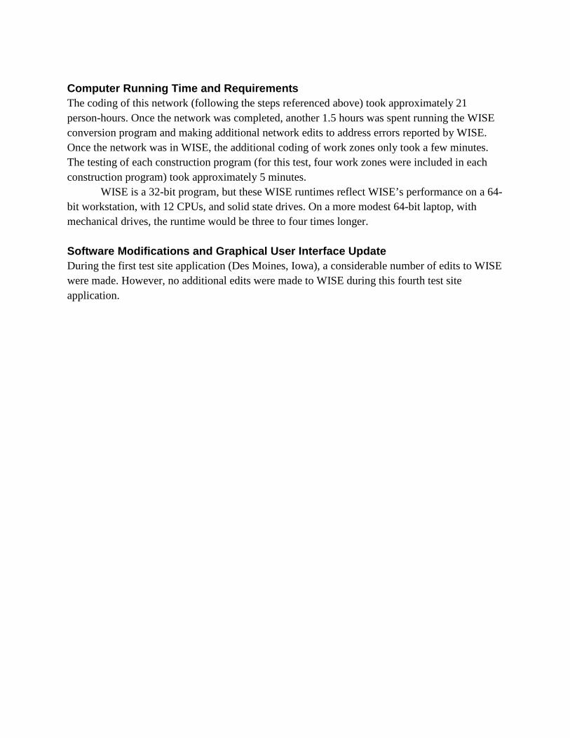
Computer Running Time and Requirements The coding of this network (following the steps referenced above) took approximately 21 person-hours. Once the network was completed, another 1.5 hours was spent running the WISE conversion program and making additional network edits to address errors reported by WISE. Once the network was in WISE, the additional coding of work zones only took a few minutes. The testing of each construction program (for this test, four work zones were included in each construction program) took approximately 5 minutes.
WISE is a 32-bit program, but these WISE runtimes reflect WISE’s performance on a 64-bit workstation, with 12 CPUs, and solid state drives. On a more modest 64-bit laptop, with mechanical drives, the runtime would be three to four times longer.
Software Modifications and Graphical User Interface Update During the first test site application (Des Moines, Iowa), a considerable number of edits to WISE were made. However, no additional edits were made to WISE during this fourth test site application.

CHAPTER 6 Conclusion and Summary Recommendations Phase 4 validation and pilot tests were conducted by a team of modelers completely independent from the initial developers of the WISE software in order to provide an objective assessment and realistic test of the developed tool on different networks and in different situations. The tests have identified strengths in the WISE tool as well as challenges that users will encounter in using the tool. It is recommended that the implementation challenges for users should be corrected in a future phase or as part of a private sector initiative to enhance and deploy the tool to facilitate wider dissemination and use of the positive features of the WISE tool.
WISE is envisioned to be used to develop and sequence programs of renewal projects in the Planning Module and to assist in the application of the “Work Zone Rule” in the Operation Module. The WISE tool includes both Planning and Operation Modules and may be applied over relatively large networks or upon complex corridors, with some restrictions as identified below that can be corrected in a future phase. The WISE software tool uses basic network geometry (link/node and number of lanes) and basic traffic volume information from virtually any platform once it is converted to a NEXTA format. Detailed instructions for conversion of network and traffic data into NEXTA formats are included in the User Guide provided as part of this project. This report documents experiences and challenges in converting existing networks to the required nonproprietary NEXTA format.
In the Planning Module, static assignment (user supplied or WISE supplied) is coupled with information on the planning characteristics of the program, a user-defined library of demand-based and duration-based renewal strategies, and basic project information. Optimal project sequencing is developed based on user and agency costs. Traffic diversion resulting from projects can be computed by WISE or entered manually for each project by the user. Later, or in parallel, in the Operation Module, the operational software (TransModeler, the DynusT dynamic traffic assignment model, or another traffic simulation platform as chosen by the user) will also compute a diversion of traffic that is based on more specific work zone information. The user can use his or her choice of operational software at the microscopic (or macroscopic) level to model projects and identify traffic diversion and manually enter the diversion into the Planning Module to develop an optimized sequence of projects and construction strategies. The graphical user interface includes a number of validation checks as well as user support features.
The WISE software has been improved in the validation and pilot tests in Phase 4 of this project. Phase 4 has provided the opportunity to test and improve the stability and rigor of the WISE code and to identify deployment challenges and desirable improvements to increase the utility of the WISE tool.

Summary of Phase 4 Findings and Recommendations WISE was deliberately built on a platform of nonproprietary software to enable its free distribution. The underlying network platform, NEXTA, has substantial limitations that were not identified until the validation and pilot tests were undertaken. WISE was developed to work on a NEXTA network for the island of Guam, consisting of two-way streets and intersections, without highways, ramps, or one-way roads. Therefore, users are required to convert their existing network to a two-way configuration with intersections or develop such a “stick network” following the directions in the User Guide.
Recommendation 1. A desirable future improvement would be to modify the WISE tool to interface directly with virtually any commercial or nonproprietary network system rather than require the users to convert their networks to meet the WISE specifications for a NEXTA network. This would enable WISE to easily evaluate large projects on Interstates and large corridors.
WISE considers a single construction project as occurring on a single highway segment. The software does not have the ability to consider that a construction project might involve numerous roadway segments.
Recommendation 2. Increase WISE’s flexibility in defining construction project scales in regard to highway segments.
WISE is limited in the number of zones and nodes that can be considered. Recommendation 3. Increase the capacity of WISE to handle more zones.
Once a project is completed, the WISE program does not set the capacity back to 100%. In fact, some projects increase capacity, and the program does not have the ability to recognize that the capacity has increased. This may or may not affect the timing and optimization of project segments.
Recommendation 4. Investigate and test the capacity algorithms and default settings in WISE and correct deficiencies.
The WISE tool is successful in setting optimized time frames for a set of work zone projects; it is successful in identifying user costs based on delay and diversion plus agency costs for different projects. It is also successful in discerning between differing construction and public involvement strategies. However, the Planning Module estimates for diversion are not robust;

user-supplied estimates of diversion will be better in most cases, and diversion estimates developed by running a microsimulation model will be even better.
Recommendation 5: Perform additional testing and development for the diversion estimates developed in the Planning Module. Develop functionality for feedback from the user’s network model, as described in Recommendation 1.
Proprietary software developers may be able to expand and improve the operation of
WISE. As currently designed, state departments of transportation may find value in using WISE within the limits described while knowing its capabilities.
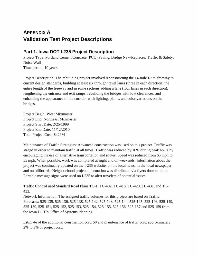
APPENDIX A Validation Test Project Descriptions Part 1. Iowa DOT I-235 Project Description Project Type: Portland Cement Concrete (PCC) Paving, Bridge New/Replaces, Traffic & Safety, Noise Wall Time period: 10 years Project Description: The rebuilding project involved reconstructing the 14-mile I-235 freeway to current design standards, building at least six through travel lanes (three in each direction) the entire length of the freeway and in some sections adding a lane (four lanes in each direction), lengthening the entrance and exit ramps, rebuilding the bridges with low clearances, and enhancing the appearance of the corridor with lighting, plants, and color variations on the bridges. Project Begin: West Mixmaster Project End: Northeast Mixmaster Project Start Date: 2/25/1999 Project End Date: 11/12/2010 Total Project Cost: $429M Maintenance of Traffic Strategies: Advanced construction was used on this project. Traffic was staged in order to maintain traffic at all times. Traffic was reduced by 10% during peak hours by encouraging the use of alternative transportation and routes. Speed was reduced from 65 mph to 55 mph. When possible, work was completed at night and on weekends. Information about the project was continually updated on the I-235 website, on the local news, in the local newspaper, and on billboards. Neighborhood project information was distributed via flyers door-to-door. Portable message signs were used on I-235 to alert travelers of potential issues. Traffic Control used Standard Road Plans TC-1, TC-402, TC-418, TC-420, TC-431, and TC-433. Network Information: The assigned traffic volumes for this project are based on Traffic Forecasts: 525-135, 525-136, 525-138, 525-142, 525-143, 525-144, 525-145, 525-146, 525-149, 525-150, 525-151, 525-152, 525-153, 525-154, 525-155, 525-156, 525-157 and 525-159 from the Iowa DOT’s Office of Systems Planning. Estimate of the additional construction cost: $0 and maintenance of traffic cost: approximately 2% to 3% of project cost.

Phase 1: Interchanges Maintenance of Traffic Strategies: Traffic was staged in order to maintain traffic on I-235 at all times. Speed was reduced from 65 mph to 55 mph. One lane of traffic in each direction was maintained on the crossroad. I-235 lane closures were permitted on nights and weekends. The construction phase lasted approximately 120 days. Traffic: 24,682 (2002) Construction Start Date: 05/30/2005 Construction End Date: 11/11/2005 Total Project Cost: $4.725M Delays: There were many rear-end crashes and congestion observed on the I-235 corridor project. Phase 2: Median Widening Maintenance of Traffic Strategies: Traffic was staged in order to maintain traffic on I-235 at all times. Speed was reduced from 65 mph to 55 mph. Lane closures were permitted on nights and weekends. The construction phase lasted approximately 170 days. Traffic: 93,400 (2005) Construction Start Date: 03/17/2004 Construction End Date: 11/12/2004 Total Project Cost: $6.24M Delays: There were many rear-end crashes and congestion observed on the I-235 corridor project. Phase 3: PCC—Eastbound Maintenance of Traffic Strategies: Traffic was staged in order to maintain 2 lanes of traffic in each direction on I-235 at all times. Speed was reduced from 65 mph to 55 mph. Lane closures were permitted on nights and weekends. The construction phase lasted approximately 258 days. Traffic: 86,332 (2000) Construction Start Date: 11/23/2005 Construction End Date: 11/17/2006 Total Project Cost: $69M

Delays: There were many rear-end crashes and congestion observed on the I-235 corridor project. Phase 4: PCC—Westbound Maintenance of Traffic Strategies: Traffic was staged in order to maintain traffic on I-235 at all times. Speed was reduced from 65 mph to 55 mph. Lane closures were permitted on nights and weekends. The construction phase lasted approximately 180 days. Traffic: 118,824 (2000) Construction Start Date: 03/13/2006 Construction End Date: 11/17/2006 Total Project Cost: $69M Delays: There were many rear-end crashes and congestion observed on the I-235 corridor project.

Part 2. Phoenix, Arizona, Project Descriptions Project A 202L Red Mountain Freeway—101L to Gilbert Road. three-lane freeway, adding HOV lane Project Start Date: 3/10/2009 Project End Date: 8/27/2010 (Open to Traffic) Project Phase Start and End Dates: Reduced and restriped all three travel lanes from 12 feet to 11 feet. Reduced the median shoulder from 8 feet to 2 feet and the outside shoulder from 10 feet to 4 feet. This was the traffic set for the duration of the project. Maintenance of Traffic Strategies: All lanes were restriped with a full weekend freeway closure. Two full closures were used (half of the project length) on two consecutive weekends to accomplish the lane shift. The ARACFC (asphalt-rubber asphaltic concrete friction course) paving was completed during weekend single lane restrictions. Cost: All traffic control costs were as planned/scheduled. There was no delay in completion due to the implementation of these strategies. Total Project Cost: $23,526,647.03 Traffic: Unknown Delays: During the initial full freeway closure of 202L westbound (WB) at Gilbert/McDowell Road to shift lanes, queues were observed in excess of 1 mile. This was due to inadequate queue space for the detour left-turn movement at the intersection. This delay was rectified during the full freeway closure to shift lanes back into their final configuration by restriping and re-signing the intersection to add an additional left turn lane as well as by modifying the associated signal time.
Project B 202L Santan Freeway—I-10 to Gilbert Road. three-lane freeway, adding HOV lane, and corresponding HOV directional ramps at I-10 and 101L
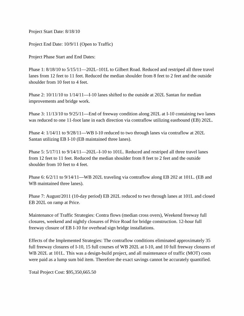
Project Start Date: 8/18/10 Project End Date: 10/9/11 (Open to Traffic) Project Phase Start and End Dates: Phase 1: 8/18/10 to 5/15/11—202L–101L to Gilbert Road. Reduced and restriped all three travel lanes from 12 feet to 11 feet. Reduced the median shoulder from 8 feet to 2 feet and the outside shoulder from 10 feet to 4 feet. Phase 2: 10/11/10 to 1/14/11—I-10 lanes shifted to the outside at 202L Santan for median improvements and bridge work. Phase 3: 11/13/10 to 9/25/11—End of freeway condition along 202L at I-10 containing two lanes was reduced to one 11-foot lane in each direction via contraflow utilizing eastbound (EB) 202L. Phase 4: 1/14/11 to 9/28/11—WB I-10 reduced to two through lanes via contraflow at 202L Santan utilizing EB I-10 (EB maintained three lanes). Phase 5: 5/17/11 to 9/14/11—202L–I-10 to 101L. Reduced and restriped all three travel lanes from 12 feet to 11 feet. Reduced the median shoulder from 8 feet to 2 feet and the outside shoulder from 10 feet to 4 feet. Phase 6: 6/2/11 to 9/14/11—WB 202L traveling via contraflow along EB 202 at 101L. (EB and WB maintained three lanes). Phase 7: August/2011 (10-day period) EB 202L reduced to two through lanes at 101L and closed EB 202L on ramp at Price. Maintenance of Traffic Strategies: Contra flows (median cross overs), Weekend freeway full closures, weekend and nightly closures of Price Road for bridge construction. 12-hour full freeway closure of EB I-10 for overhead sign bridge installations. Effects of the Implemented Strategies: The contraflow conditions eliminated approximately 35 full freeway closures of I-10, 15 full courses of WB 202L at I-10, and 10 full freeway closures of WB 202L at 101L. This was a design-build project, and all maintenance of traffic (MOT) costs were paid as a lump sum bid item. Therefore the exact savings cannot be accurately quantified. Total Project Cost: $95,350,665.50

Traffic: Unknown Delays: While shifting WB I-10 traffic into the contraflow configuration, one through lane was maintained at all times. This caused a queue of approximately 2 miles to the south during the morning hours of a Saturday. Project C SR 101 HOV Addition—SR 202 Red Mountain to Princess Drive Project Start Date: 8/27/07 Project End Date: 1/5/10 Project Phase Start and End Dates: 9/20/07—restriped NB 101 from 202 to Chaparral. Reduced lane widths to 11 feet. Returned traffic to their own lanes including HOV 11/10/08. 9/28/07—restriped SB 101 from 202 to Chaparral. Reduced lane widths to 11 feet. Returned traffic to their own lanes including HOV 11/10/08. 10/26/07—restriped NB 101 from Chaparral to Shea. Reduced lane widths to 11 feet. Returned traffic to their own lanes including HOV 11/10/08 up to Via de Ventura. Via de Ventura to Shea was returned on 5/8/09. 11/2/07—restriped SB 101 from Chaparral to Shea. Reduced lane widths to 11 feet. Returned traffic to their own lanes including HOV 11/10/08 up to Via de Ventura. Via de Ventura to Shea was returned on 5/8/09. 6/20/08—restriped NB 101 from Shea to Princess. Reduced lane widths to 11 feet. Returned traffic to their own lanes including HOV 5/8/09 6/27/08—restriped SB 101 from Shea to Princess. Reduced lane widths to 11 feet. Returned traffic to their own lanes including HOV 5/8/09 Maintenance of Traffic Strategies: All lanes were restriped at night under a full closure to allow the establishment of an inside work zone. (2-11-11-11-4) Once work zone was established minimal closures were required. Detours were only used for detour full closure work. The project used a nightly closure specification that ensured that all lanes were reopened to traffic by 5 a.m. For every 5 minutes the road was not open past 5 a.m. the contractor was penalized $5,000. A website was set up to inform the traveling public of the closures. The project closely coordinated
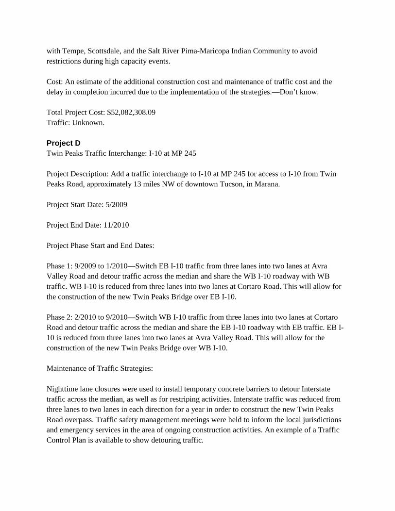
with Tempe, Scottsdale, and the Salt River Pima-Maricopa Indian Community to avoid restrictions during high capacity events. Cost: An estimate of the additional construction cost and maintenance of traffic cost and the delay in completion incurred due to the implementation of the strategies.—Don’t know. Total Project Cost: $52,082,308.09 Traffic: Unknown. Project D Twin Peaks Traffic Interchange: I-10 at MP 245 Project Description: Add a traffic interchange to I-10 at MP 245 for access to I-10 from Twin Peaks Road, approximately 13 miles NW of downtown Tucson, in Marana. Project Start Date: 5/2009 Project End Date: 11/2010 Project Phase Start and End Dates: Phase 1: 9/2009 to 1/2010—Switch EB I-10 traffic from three lanes into two lanes at Avra Valley Road and detour traffic across the median and share the WB I-10 roadway with WB traffic. WB I-10 is reduced from three lanes into two lanes at Cortaro Road. This will allow for the construction of the new Twin Peaks Bridge over EB I-10. Phase 2: 2/2010 to 9/2010—Switch WB I-10 traffic from three lanes into two lanes at Cortaro Road and detour traffic across the median and share the EB I-10 roadway with EB traffic. EB I-10 is reduced from three lanes into two lanes at Avra Valley Road. This will allow for the construction of the new Twin Peaks Bridge over WB I-10. Maintenance of Traffic Strategies: Nighttime lane closures were used to install temporary concrete barriers to detour Interstate traffic across the median, as well as for restriping activities. Interstate traffic was reduced from three lanes to two lanes in each direction for a year in order to construct the new Twin Peaks Road overpass. Traffic safety management meetings were held to inform the local jurisdictions and emergency services in the area of ongoing construction activities. An example of a Traffic Control Plan is available to show detouring traffic.

Cost: The exact costs for maintenance and protection of traffic (MPT) would be difficult to determine; however, the total Arizona DOT cost associated with MPT was $1.13M with the temporary concrete barrier costing over $900,000. Total Project Cost: $52.5M Traffic: The average daily traffic (ADT) for I-10 in this area is 72,000 according to the Pima Association of Governments (PAG). Twin Peaks Road is a new alignment, so there is limited data available for it. Delays: Some delays occurred during the nighttime closures when setting up and taking down the lane closure traffic control. There were delays on the weekends that were used to set up and detour traffic across the I-10 median. There were four weekends (Friday 9 a.m. to Monday 5 a.m.) during which I-10 traffic (EB and WB) was reduced from three lanes to one lane to install a temporary concrete barrier (TCB) and restripe. This caused significant delays for traveling motorists. There were several accidents on the project site that also caused significant delays. Project E I-10 Kino Boulevard to Valencia Road Project Start Date: 1/2011 Project End Date: 10/2011 Project Phase Start and End Dates: No phasing was used for this project. Maintenance of Traffic Strategies: Nighttime work was a must. Lane closures occurred from 7 p.m. to 6 a.m. We had to reconstruct the PCC pavement slabs on mainline I-10 in both the EB and WB directions, so a high-early concrete was used in order to open the freeway by the 6 a.m. time specification. The Arizona DOT enforced specifications penalties of $3,000 per hour for WB I-10 and $1,800 for EB I-10 and $200 per hour for ramps when the time limits were not adhered to by the contractor. When ramp work was necessary, the ramps were closed during the same time frame durations, and traffic was rerouted. Cost (an estimate of the additional construction cost and maintenance of traffic cost and the delay in completion incurred due to the implementation of the strategies): unknown. A cost analysis would need to be prepared to analyze the effects of closing the lanes down during the day or adding a third lane. The project was very limited in its options because there are only two lanes in each direction on I-10 in this location. The total MPT cost was $427,000. However, as

indicated by the contractor, the amount paid to the contractor for MPT costs does not necessarily cover all the costs borne by the contractor to the traffic control companies because of mobilization payments. Total Project Cost : $6.1M Traffic: Unknown. PAG shows 62,000 to 80,000 annual ADT. Delays: In general, the lanes would be closed down at 7 p.m., and traffic would begin to back up. The wait times to get through the project ranged from 5 to 10 minutes. By 10 p.m. or 11 p.m. the queues would have dissipated and the freeway would be operating at the posted speed with one lane closed.
Project F Project Description: 202 Red Mountain Design Build—General Purpose addition EB I-10 to 101, WB 101 to Scottsdale Road Project Start Date: 12/17/08 Project End Date: 6/17/11 Project Phase Start and End Dates: (Phases would be when significant changes in capacity occurred during construction – minimum time for a phase would be 30 days.) 40th Street Ramp B Closure: 6/1/09 to 7/15/09 32nd Street Ramp B Closure: 7/15/09 to 9/15/09 52nd Street Ramp B Closure: 7/15/09 to 9/15/09 24th Street Ramp B Closure: 1/14/10 to 3/4/10 44th Street Ramp D: 6/25/09 to 8/23/09 32nd Street Ramp D: 8/23/09 to 10/23/09 Van Buren Ramp S: 8/23/09 to 10/23/09 24th St Ramp D: 1/14/10 to 3/4/10

Maintenance of Traffic Strategies: The contract was bid to keep three lanes of mainline traffic and one ramp lane open. During development of the traffic control plans, the contractor proposed to close eight of the ramps. The closures would allow quicker completion of the ramps with higher quality pavement because of minimized jointing in the PCC pavement. This strategy saved the state $441,940.48. Cost: An estimate of the additional construction cost and maintenance of traffic cost and the delay in completion incurred by the implementation of the strategies. The proposed strategies saved the contract both time and money as well as inconvenience to the traveling public. Total Project Cost: $190,860,756.57 Traffic: Unknown Delays: Unknown

APPENDIX B Pilot Test Project Descriptions
Orlando, Florida, Proposed Project Descriptions The I-4, SR 400 widening full project alternative will extend from west of Kirkman Road in Orange County to east of SR 434 in Seminole County. I-4 will be reconstructed to accommodate three general use lanes, auxiliary lanes, and two managed lanes in the eastbound and westbound directions. Access to and from the managed lanes will be provided through slip ramps located along the corridor and direct access ramps at Grand National Drive, Anderson Street, South Street, Ivanhoe Boulevard, and Central Parkway interchanges. The SR 408/I-4 interchange will be built to its ultimate configuration and will include modifications to SR 408, which is operated by the Orlando-Orange County Expressway Authority. The improvements to SR 408 will include, but not be limited to, modifications or additions of bridges over the following:
1. Parramore Avenue 2. Westmoreland Avenue 3. Rio Grande Avenue 4. Orange Blossom Trail 5. Tampa Avenue
The widening of I-4 includes reconstruction of the following interchanges:
1. Kirkman Road 2. Orange Blossom Trail 3. Michigan Avenue 4. Kaley Street 5. SR 408 6. SR 50 7. Ivanhoe Boulevard 8. Park Avenue 9. Princeton Street 10. Fairbanks Avenue 11. Lee Road 12. Maitland Boulevard 13. SR 436 14. SR 434
All bridges that are part of I-4 are being replaced within the limits of the project.

APPENDIX C TransCAD GISDK Scripts Part 1. Iowa Validation TransCAD GISDK Script Macro "Batch Macro" RunMacro("TCB Init") ProjectPath ="D:\\Projects\\Iowa\\TransCAD_Network\\" OutputPath = ProjectPath + "output\\" Network_File = ProjectPath + "Network_303.dbd" {node_lyr, link_lyr} = RunMacro("TCB Add DB Layers", Network_File,,) NumberOfZones = 55 // ********************* zone.dat rpt = OpenFile(OutputPath+"zone.dat","w") ZSort = {{"Sort Order", {{"ID", "Ascending"}}}} Writeline(rpt, "This file defines zone regions") Writeline(rpt, "number of feature points, number of zones") SetLayer(node_lyr) n = SelectByQuery("TAZ_Set", "Several", "Select * where ID<>null", ) {V_ID, V_Longitude, V_Latitude, V_TAZ, V_x, V_y} = GetDataVectors(node_lyr+"|TAZ_Set", {"ID", "Longitude", "Latitude", "TAZ_ID_Tag","x","y"}, ZSort) V_x = 1000000000+V_Longitude V_y = V_Latitude-40000000 Writeline(rpt, " "+i2s(V_ID.length)+" "+i2s(NumberOfZones)) Writeline(rpt, "node #, x-coordinate, y-coordinate") for i=1 to V_ID.length do Anode = i2s(V_ID[i]) for j=len(Anode) to 6 do Anode = " "+Anode end Long = r2s(V_x[i]) for j=len(Long) to 15 do Long = " "+Long end Latt = r2s(V_y[i]) for j=len(Latt) to 15 do Latt = " "+Latt end Writeline(rpt,Anode+Long+","+Latt) end Writeline(rpt, "zone #, number of nodes, node #'s") for i=1 to NumberOfZones do SetLayer(node_lyr) n = SelectByQuery("TAZ_Set", "Several", "Select * where TAZ_ID_Tag="+i2s(i), ) {V_ID, V_Longitude, V_Latitude} = GetDataVectors(node_lyr+"|TAZ_Set", {"ID", "Longitude", "Latitude"}, ZSort) i_string = i2s(i) for j=Len(i_string) to 6 do i_string = " "+i_string end Line2Print = i_string cnt = i2s(V_ID.length-1) for j=Len(cnt) to 7 do cnt = " "+cnt end Line2Print = Line2Print+cnt+":" for j=2 to V_ID.length do if j=2 then do node = i2s(V_ID[j]) for k=Len(node) to 7 do node = " "+node end end else do node = i2s(V_ID[j]) for k=Len(node) to 6 do node = " "+node end end if j<V_ID.length then Line2Print = Line2Print + node+","

else Line2Print = Line2Print + node end Writeline(rpt,Line2Print) end CloseFile(rpt) // **************************** xy dat rpt = OpenFile(OutputPath+"xy.dat","w") {V_ID, V_Longitude, V_Latitude} = GetDataVectors(node_lyr+"|", {"ID", "Longitude", "Latitude"}, ZSort) for i=1 to V_ID.length do i_string = i2s(V_ID[i]) for j=Len(i_string) to 6 do i_string = " "+i_string end Line2Print = i_string xrval = Round(V_x[i],3) x_string = r2s(xrval) if Len(x_string)<10 then x_string=x_string+"0" if Len(x_string)<10 then x_string=x_string+"0" for j=Len(x_string) to 15 do x_string = " "+x_string end Line2Print = x_string yrval = Round(V_y[i],3) y_string = r2s(yrval) if Len(y_string)<10 then y_string=y_string+"0" if Len(y_string)<10 then y_string=y_string+"0" for j=Len(y_string) to 15 do y_string = " "+y_string end Line2Print = y_string Writeline(rpt,i_string + x_string + y_string) end CloseFile(rpt) // ************************** static import {V_Dir, V_Length, V_A_Node, V_B_Node, V_AB_Time_2005UE, V_BA_Time_2005UE, V_AB_Flow_2005UE, V_BA_Flow_2005UE, V_VCR02, V_FFSPEED} = GetDataVectors(link_lyr+"|", {"Dir", "Length", "A_Node", "B_Node", "AB_CongTime", "BA_CongTime", "AB_Flow", "BA_Flow", "VCR02", "FFSPEED"}, {{"Sort Order", {{"A_Node", "Ascending"}}}}) V_VCR02 = nz(V_VCR02) V_VCR02 = if V_VCR02=0 then 1 else V_VCR02 V_AB_Time_2005UE = ((V_Length/V_FFSPEED)*60) * (1+0.15*POW(V_VCR02,4)) skip_Zone: rpt2 = OpenFile(OutputPath+"Static_Import2.csv","w") // Midday, Night-time split is 60/40 Sp_MD=0.67 Sp_NT=0.33 MD_PK=0.12 NT_PK=0.08 writeline(rpt2, "FROM_ID,TO_ID,DAY_TIME,NIGHT_TIME,DAY_FLOW,NIGHT_FLOW") for i=1 to V_Dir.length do if V_Dir[i]>-1 then writeline(rpt2, i2s(V_A_Node[i])+","+i2s(V_B_Node[i])+","+r2s(V_AB_Time_2005UE[i])+","+r2s(V_AB_Time_2005UE[i])+","+r2s(V_AB_Flow_2005UE[i]*Sp_MD*MD_PK)+","+r2s(V_AB_Flow_2005UE[i]*Sp_NT*NT_PK)) if V_Dir[i]<1 then writeline(rpt2, i2s(V_B_Node[i])+","+i2s(V_A_Node[i])+","+r2s(V_BA_Time_2005UE[i])+","+r2s(V_BA_Time_2005UE[i])+","+r2s(V_BA_Flow_2005UE[i]*Sp_MD*MD_PK)+","+r2s(V_BA_Flow_2005UE[i]*Sp_NT*NT_PK))

end CloseFile(rpt2) // *********************** workzone.dat rpt3 = OpenFile(OutputPath+"WorkZone.dat","w") SetLayer(link_lyr) n = SelectByQuery("Work_Set", "Several", "Select * where WorkZone="+i2s(1), ) {V_Dir, V_Length, V_A_Node, V_B_Node, V_AB_Time, V_BA_Time, V_AB_Flow, V_BA_Flow, V_AB_Lanes, V_BA_Lanes, V_FFSpeed, V_AB_LANECAP, V_BA_LANECAP, V_FEDFUNC} = GetDataVectors(link_lyr+"|Work_Set", {"Dir", "Length", "A_Node", "B_Node", "AB_CongTime", "BA_CongTime", "AB_Flow", "BA_Flow", "AB_Lanes", "BA_Lanes", "FFSPEED", "AB_LANECAP" , "BA_LANECAP", "FEDFUNC"}, ) Writeline(rpt3, i2s(V_Dir.length)) for i=1 to V_Dir.length do Writeline(rpt3, i2s(V_A_Node[i])+" "+i2s(V_B_Node[i])+" 0 1440 0.5 30 1500") end Writeline(rpt3,"") CloseFile(rpt3) rpt4 = OpenFile(OutputPath+"network.dat","w") SetLayer(node_lyr) n = SelectByQuery("TAZ_Set", "Several", "Select * where ID<>null", ) {V_ID, V_Longitude, V_Latitude, V_TAZ} = GetDataVectors(node_lyr+"|TAZ_Set", {"ID", "Longitude", "Latitude", "TAZ_ID_Tag"}, ZSort) {V_Dir, V_Length, V_A_Node, V_B_Node, V_AB_Time_2005UE, V_BA_Time_2005UE, V_AB_Flow_2005UE, V_BA_Flow_2005UE, V_AB_Lanes, V_BA_Lanes, V_FFSpeed, V_AB_LANECAP, V_BA_LANECAP, V_FEDFUNC} = GetDataVectors(link_lyr+"|", {"Dir", "Length", "A_Node", "B_Node", "AB_CongTime", "BA_CongTime", "AB_Flow", "BA_Flow", "AB_LANES", "BA_LANES", "FFSPEED", "AB_LANECAP" , "BA_LANECAP", "FEDFUNC"}, ) nodes=V_Longitude.length links=0 for i=1 to V_Dir.length do if V_Dir[i]=0 then links = links+2 if V_Dir[i]=1 or V_Dir[i]=-1 then links=links+1 end zone_string = r2s(NumberOfZones) for j=Len(zone_string) to 6 do zone_string = " "+zone_string end nodes_string = r2s(nodes) for j=Len(nodes_string) to 6 do nodes_string = " "+nodes_string end links_string = r2s(links) for j=Len(links_string) to 6 do links_string = " "+links_string end Writeline(rpt4, zone_string+nodes_string+links_string+" 1 0") For i=1 to nodes do Anode = i2s(V_ID[i]) for j=len(Anode) to 6 do Anode = " "+Anode end Bnode = i2s(V_TAZ[i]) for j=len(Bnode) to 4 do Bnode = " "+Bnode end Writeline(rpt4,Anode+Bnode) end

sort_vw = RunMacro("TCB OpenTable",,,{ProjectPath+"Network_Sort.bin"}) {V_A, V_B, V_A_C, V_D, V_E, V_F, V_G, V_H, V_I, V_J, V_K, V_L, V_M} = GetDataVectors(sort_vw+"|", {"C_A", "C_B", "C_C", "C_D", "C_E", "C_F", "C_G", "C_H", "C_I", "C_J", "C_K", "C_L" , "C_M"}, ) For i=1 to V_A.length do Anode = i2s(V_A[i]) for j=len(Anode) to 6 do Anode = " "+Anode end Bnode = i2s(V_B[i]) for j=len(Bnode) to 6 do Bnode = " "+Bnode end dist = i2s(V_E[i]) for j=len(dist) to 6 do dist = " " + dist end lanes = i2s(V_F[i]) for j=len(lanes) to 2 do lanes = " " + lanes end speed = i2s(V_I[i]) for j=len(speed) to 3 do speed = " "+speed end ABcap_string = i2s(V_J[i]) for j=len(ABcap_string) to 5 do ABcap_string = " " + ABcap_string end BAcap_string = i2s(V_K[i]) for j=len(BAcap_string) to 5 do BAcap_string = " " + BAcap_string end func = i2s(V_L[i]) for j=len(func) to 2 do func = " " +func end Writeline(rpt4, Anode+Bnode+ " 0 0" + dist+lanes+ " 2 +0"+speed+ABcap_string+" 1800"+func+" +0") end CloseFile(rpt4) ok=1 quit: Return( RunMacro("TCB Closing", ok, True ) ) endMacro

Part 2. Phoenix, Arizona, TransCAD GISDK Script Macro "Batch Macro" ProjectPath ="D:\\Projects\\Phoenix\\Model\\TransCAD\\" OutputPath ="D:\\Projects\\Phoenix\\Model\\Output\\" Network_File = ProjectPath + "Base_Network_07.dbd" {node_lyr, link_lyr} = RunMacro("TCB Add DB Layers", Network_File,,) NumberOfZones = 84 // ********************* zone.dat rpt = OpenFile(OutputPath+"zone.dat","w") ZSort = {{"Sort Order", {{"ID", "Ascending"}}}} Writeline(rpt, "This file defines zone regions") Writeline(rpt, "number of feature points, number of zones") SetLayer(node_lyr) n = SelectByQuery("TAZ_Set", "Several", "Select * where ID<>null", ) {V_ID, V_Longitude, V_Latitude, V_TAZ, V_x, V_y} = GetDataVectors(node_lyr+"|TAZ_Set", {"ID", "Longitude", "Latitude", "TAZ_ID_Tag","x","y"}, ZSort) V_x = 1000000000+V_Longitude V_y = V_Latitude-40000000 Writeline(rpt, " "+i2s(V_ID.length)+" "+i2s(NumberOfZones)) Writeline(rpt, "node #, x-coordinate, y-coordinate") for i=1 to V_ID.length do Anode = i2s(V_ID[i]) for j=len(Anode) to 6 do Anode = " "+Anode end Long = r2s(V_x[i]) for j=len(Long) to 15 do Long = " "+Long end Latt = r2s(V_y[i]) for j=len(Latt) to 15 do Latt = " "+Latt end Writeline(rpt,Anode+Long+","+Latt) end Writeline(rpt, "zone #, number of nodes, node #'s") for i=1 to NumberOfZones do SetLayer(node_lyr) n = SelectByQuery("TAZ_Set", "Several", "Select * where TAZ_ID_Tag="+i2s(i), ) {V_ID, V_Longitude, V_Latitude} = GetDataVectors(node_lyr+"|TAZ_Set", {"ID", "Longitude", "Latitude"}, ZSort) i_string = i2s(i) for j=Len(i_string) to 6 do i_string = " "+i_string end Line2Print = i_string cnt = i2s(V_ID.length-1) for j=Len(cnt) to 7 do cnt = " "+cnt end Line2Print = Line2Print+cnt+":" for j=2 to V_ID.length do if j=2 then do node = i2s(V_ID[j]) for k=Len(node) to 7 do node = " "+node end end else do node = i2s(V_ID[j]) for k=Len(node) to 6 do node = " "+node end end if j<V_ID.length then Line2Print = Line2Print + node+"," else Line2Print = Line2Print + node end Writeline(rpt,Line2Print) end CloseFile(rpt)

// **************************** xy dat rpt = OpenFile(OutputPath+"xy.dat","w") {V_ID, V_Longitude, V_Latitude} = GetDataVectors(node_lyr+"|", {"ID", "Longitude", "Latitude"}, ZSort) for i=1 to V_ID.length do i_string = i2s(V_ID[i]) for j=Len(i_string) to 6 do i_string = " "+i_string end Line2Print = i_string xrval = Round(V_x[i],3) x_string = r2s(xrval) if Len(x_string)<10 then x_string=x_string+"0" if Len(x_string)<10 then x_string=x_string+"0" for j=Len(x_string) to 15 do x_string = " "+x_string end Line2Print = x_string yrval = Round(V_y[i],3) y_string = r2s(yrval) if Len(y_string)<10 then y_string=y_string+"0" if Len(y_string)<10 then y_string=y_string+"0" for j=Len(y_string) to 15 do y_string = " "+y_string end Line2Print = y_string Writeline(rpt,i_string + x_string + y_string) end CloseFile(rpt) // ************************** static import {V_Dir, V_Length, V_A_Node, V_B_Node, V_AB_Time_2005UE, V_BA_Time_2005UE, V_AB_Flow_2005UE, V_BA_Flow_2005UE, V_VCR02, V_FFSPEED} = GetDataVectors(link_lyr+"|", {"Dir", "Length", "A_Node", "B_Node", "AB_CongTime", "BA_CongTime", "AB_Flow", "BA_Flow", "VCR02", "FFSPEED"}, {{"Sort Order", {{"A_Node", "Ascending"}}}}) V_VCR02 = nz(V_VCR02) V_VCR02 = if V_VCR02=0 then 1 else V_VCR02 V_AB_Time_2005UE = ((V_Length/V_FFSPEED)*60) * (1+0.15*POW(V_VCR02,4)) skip_Zone: rpt2 = OpenFile(OutputPath+"Static_Import2.csv","w") // Midday, Night-time split is 60/40 Sp_MD=0.67 Sp_NT=0.33 MD_PK=0.12 NT_PK=0.08 writeline(rpt2, "FROM_ID,TO_ID,DAY_TIME,NIGHT_TIME,DAY_FLOW,NIGHT_FLOW") for i=1 to V_Dir.length do if V_Dir[i]>-1 then writeline(rpt2, i2s(V_A_Node[i])+","+i2s(V_B_Node[i])+","+r2s(V_AB_Time_2005UE[i])+","+r2s(V_AB_Time_2005UE[i])+","+r2s(V_AB_Flow_2005UE[i]*Sp_MD*MD_PK)+","+r2s(V_AB_Flow_2005UE[i]*Sp_NT*NT_PK)) if V_Dir[i]<1 then writeline(rpt2, i2s(V_B_Node[i])+","+i2s(V_A_Node[i])+","+r2s(V_BA_Time_2005UE[i])+","+r2s(V_BA_Time_2005UE[i])+","+r2s(V_BA_Flow_2005UE[i]*Sp_MD*MD_PK)+","+r2s(V_BA_Flow_2005UE[i]*Sp_NT*NT_PK)) end CloseFile(rpt2) // *********************** workzone.dat rpt3 = OpenFile(OutputPath+"WorkZone.dat","w") SetLayer(link_lyr)

n = SelectByQuery("Work_Set", "Several", "Select * where WorkZone="+i2s(1), ) {V_Dir, V_Length, V_A_Node, V_B_Node, V_AB_Time, V_BA_Time, V_AB_Flow, V_BA_Flow, V_AB_Lanes, V_BA_Lanes, V_FFSpeed, V_AB_LANECAP, V_BA_LANECAP, V_FEDFUNC} = GetDataVectors(link_lyr+"|Work_Set", {"Dir", "Length", "A_Node", "B_Node", "AB_CongTime", "BA_CongTime", "AB_Flow", "BA_Flow", "AB_Lanes", "BA_Lanes", "FFSPEED", "AB_LANECAP" , "BA_LANECAP", "FEDFUNC"}, ) Writeline(rpt3, i2s(V_Dir.length)) for i=1 to V_Dir.length do Writeline(rpt3, i2s(V_A_Node[i])+" "+i2s(V_B_Node[i])+" 0 1440 0.5 30 1500") end Writeline(rpt3,"") CloseFile(rpt3) rpt4 = OpenFile(OutputPath+"network.dat","w") SetLayer(node_lyr) n = SelectByQuery("TAZ_Set", "Several", "Select * where ID<>null", ) {V_ID, V_Longitude, V_Latitude, V_TAZ} = GetDataVectors(node_lyr+"|TAZ_Set", {"ID", "Longitude", "Latitude", "TAZ_ID_Tag"}, ZSort) {V_Dir, V_Length, V_A_Node, V_B_Node, V_AB_Time_2005UE, V_BA_Time_2005UE, V_AB_Flow_2005UE, V_BA_Flow_2005UE, V_AB_Lanes, V_BA_Lanes, V_FFSpeed, V_AB_LANECAP, V_BA_LANECAP, V_FEDFUNC} = GetDataVectors(link_lyr+"|", {"Dir", "Length", "A_Node", "B_Node", "AB_CongTime", "BA_CongTime", "AB_Flow", "BA_Flow", "AB_LANES", "BA_LANES", "FFSPEED", "AB_LANECAP" , "BA_LANECAP", "FEDFUNC"}, ) nodes=V_Longitude.length links=0 for i=1 to V_Dir.length do if V_Dir[i]=0 then links = links+2 if V_Dir[i]=1 or V_Dir[i]=-1 then links=links+1 end zone_string = r2s(NumberOfZones) for j=Len(zone_string) to 6 do zone_string = " "+zone_string end nodes_string = r2s(nodes) for j=Len(nodes_string) to 6 do nodes_string = " "+nodes_string end links_string = r2s(links) for j=Len(links_string) to 6 do links_string = " "+links_string end Writeline(rpt4, zone_string+nodes_string+links_string+" 1 0") For i=1 to nodes do Anode = i2s(V_ID[i]) for j=len(Anode) to 6 do Anode = " "+Anode end Bnode = i2s(V_TAZ[i]) for j=len(Bnode) to 4 do Bnode = " "+Bnode end Writeline(rpt4,Anode+Bnode) end sort_vw = RunMacro("TCB OpenTable",,,{ProjectPath+"Network_Sort.bin"}) {V_A, V_B, V_A_C, V_D, V_E, V_F, V_G, V_H, V_I, V_J, V_K, V_L, V_M} = GetDataVectors(sort_vw+"|", {"C_A", "C_B", "C_C", "C_D", "C_E", "C_F", "C_G", "C_H", "C_I", "C_J", "C_K", "C_L" , "C_M"}, ) For i=1 to V_A.length do

Anode = i2s(V_A[i]) for j=len(Anode) to 6 do Anode = " "+Anode end Bnode = i2s(V_B[i]) for j=len(Bnode) to 6 do Bnode = " "+Bnode end dist = i2s(V_E[i]) for j=len(dist) to 6 do dist = " " + dist end lanes = i2s(V_F[i]) for j=len(lanes) to 2 do lanes = " " + lanes end speed = i2s(V_I[i]) for j=len(speed) to 3 do speed = " "+speed end ABcap_string = i2s(V_J[i]) for j=len(ABcap_string) to 5 do ABcap_string = " " + ABcap_string end BAcap_string = i2s(V_K[i]) for j=len(BAcap_string) to 5 do BAcap_string = " " + BAcap_string end func = i2s(V_L[i]) for j=len(func) to 2 do func = " " +func end Writeline(rpt4, Anode+Bnode+ " 0 0" + dist+lanes+ " 2 +0"+speed+ABcap_string+" 1800"+func+" +0") end CloseFile(rpt4) ok=1 quit: Return( RunMacro("TCB Closing", ok, True ) ) endMacro

Part 3. Orlando, Florida, TransCAD GISDK Script Macro "Batch Macro" ProjectPath ="D:\\Projects\\Orlando\\Model\\TransCAD\\" OutputPath ="D:\\Projects\\Orlando\\Model\\Output\\" Network_File = ProjectPath + "Base_Network_07.dbd" {node_lyr, link_lyr} = RunMacro("TCB Add DB Layers", Network_File,,) NumberOfZones = 84 // ********************* zone.dat rpt = OpenFile(OutputPath+"zone.dat","w") ZSort = {{"Sort Order", {{"ID", "Ascending"}}}} Writeline(rpt, "This file defines zone regions") Writeline(rpt, "number of feature points, number of zones") SetLayer(node_lyr) n = SelectByQuery("TAZ_Set", "Several", "Select * where ID<>null", ) {V_ID, V_Longitude, V_Latitude, V_TAZ, V_x, V_y} = GetDataVectors(node_lyr+"|TAZ_Set", {"ID", "Longitude", "Latitude", "TAZ_ID_Tag","x","y"}, ZSort) V_x = 1000000000+V_Longitude V_y = V_Latitude-40000000 Writeline(rpt, " "+i2s(V_ID.length)+" "+i2s(NumberOfZones)) Writeline(rpt, "node #, x-coordinate, y-coordinate") for i=1 to V_ID.length do Anode = i2s(V_ID[i]) for j=len(Anode) to 6 do Anode = " "+Anode end Long = r2s(V_x[i]) for j=len(Long) to 15 do Long = " "+Long end Latt = r2s(V_y[i]) for j=len(Latt) to 15 do Latt = " "+Latt end Writeline(rpt,Anode+Long+","+Latt) end Writeline(rpt, "zone #, number of nodes, node #'s") for i=1 to NumberOfZones do SetLayer(node_lyr) n = SelectByQuery("TAZ_Set", "Several", "Select * where TAZ_ID_Tag="+i2s(i), ) {V_ID, V_Longitude, V_Latitude} = GetDataVectors(node_lyr+"|TAZ_Set", {"ID", "Longitude", "Latitude"}, ZSort) i_string = i2s(i) for j=Len(i_string) to 6 do i_string = " "+i_string end Line2Print = i_string cnt = i2s(V_ID.length-1) for j=Len(cnt) to 7 do cnt = " "+cnt end Line2Print = Line2Print+cnt+":" for j=2 to V_ID.length do if j=2 then do node = i2s(V_ID[j]) for k=Len(node) to 7 do node = " "+node end end else do node = i2s(V_ID[j]) for k=Len(node) to 6 do node = " "+node end end if j<V_ID.length then Line2Print = Line2Print + node+"," else Line2Print = Line2Print + node end Writeline(rpt,Line2Print) end CloseFile(rpt)

// **************************** xy dat rpt = OpenFile(OutputPath+"xy.dat","w") {V_ID, V_Longitude, V_Latitude} = GetDataVectors(node_lyr+"|", {"ID", "Longitude", "Latitude"}, ZSort) for i=1 to V_ID.length do i_string = i2s(V_ID[i]) for j=Len(i_string) to 6 do i_string = " "+i_string end Line2Print = i_string xrval = Round(V_x[i],3) x_string = r2s(xrval) if Len(x_string)<10 then x_string=x_string+"0" if Len(x_string)<10 then x_string=x_string+"0" for j=Len(x_string) to 15 do x_string = " "+x_string end Line2Print = x_string yrval = Round(V_y[i],3) y_string = r2s(yrval) if Len(y_string)<10 then y_string=y_string+"0" if Len(y_string)<10 then y_string=y_string+"0" for j=Len(y_string) to 15 do y_string = " "+y_string end Line2Print = y_string Writeline(rpt,i_string + x_string + y_string) end CloseFile(rpt) // ************************** static import {V_Dir, V_Length, V_A_Node, V_B_Node, V_AB_Time_2005UE, V_BA_Time_2005UE, V_AB_Flow_2005UE, V_BA_Flow_2005UE, V_VCR02, V_FFSPEED} = GetDataVectors(link_lyr+"|", {"Dir", "Length", "A_Node", "B_Node", "AB_CongTime", "BA_CongTime", "AB_Flow", "BA_Flow", "VCR02", "FFSPEED"}, {{"Sort Order", {{"A_Node", "Ascending"}}}}) V_VCR02 = nz(V_VCR02) V_VCR02 = if V_VCR02=0 then 1 else V_VCR02 V_AB_Time_2005UE = ((V_Length/V_FFSPEED)*60) * (1+0.15*POW(V_VCR02,4)) skip_Zone: rpt2 = OpenFile(OutputPath+"Static_Import2.csv","w") // Midday, Night-time split is 60/40 Sp_MD=0.67 Sp_NT=0.33 MD_PK=0.12 NT_PK=0.08 writeline(rpt2, "FROM_ID,TO_ID,DAY_TIME,NIGHT_TIME,DAY_FLOW,NIGHT_FLOW") for i=1 to V_Dir.length do if V_Dir[i]>-1 then writeline(rpt2, i2s(V_A_Node[i])+","+i2s(V_B_Node[i])+","+r2s(V_AB_Time_2005UE[i])+","+r2s(V_AB_Time_2005UE[i])+","+r2s(V_AB_Flow_2005UE[i]*Sp_MD*MD_PK)+","+r2s(V_AB_Flow_2005UE[i]*Sp_NT*NT_PK)) if V_Dir[i]<1 then writeline(rpt2, i2s(V_B_Node[i])+","+i2s(V_A_Node[i])+","+r2s(V_BA_Time_2005UE[i])+","+r2s(V_BA_Time_2005UE[i])+","+r2s(V_BA_Flow_2005UE[i]*Sp_MD*MD_PK)+","+r2s(V_BA_Flow_2005UE[i]*Sp_NT*NT_PK)) end CloseFile(rpt2) // *********************** workzone.dat rpt3 = OpenFile(OutputPath+"WorkZone.dat","w") SetLayer(link_lyr)

n = SelectByQuery("Work_Set", "Several", "Select * where WorkZone="+i2s(1), ) {V_Dir, V_Length, V_A_Node, V_B_Node, V_AB_Time, V_BA_Time, V_AB_Flow, V_BA_Flow, V_AB_Lanes, V_BA_Lanes, V_FFSpeed, V_AB_LANECAP, V_BA_LANECAP, V_FEDFUNC} = GetDataVectors(link_lyr+"|Work_Set", {"Dir", "Length", "A_Node", "B_Node", "AB_CongTime", "BA_CongTime", "AB_Flow", "BA_Flow", "AB_Lanes", "BA_Lanes", "FFSPEED", "AB_LANECAP" , "BA_LANECAP", "FEDFUNC"}, ) Writeline(rpt3, i2s(V_Dir.length)) for i=1 to V_Dir.length do Writeline(rpt3, i2s(V_A_Node[i])+" "+i2s(V_B_Node[i])+" 0 1440 0.5 30 1500") end Writeline(rpt3,"") CloseFile(rpt3) rpt4 = OpenFile(OutputPath+"network.dat","w") SetLayer(node_lyr) n = SelectByQuery("TAZ_Set", "Several", "Select * where ID<>null", ) {V_ID, V_Longitude, V_Latitude, V_TAZ} = GetDataVectors(node_lyr+"|TAZ_Set", {"ID", "Longitude", "Latitude", "TAZ_ID_Tag"}, ZSort) {V_Dir, V_Length, V_A_Node, V_B_Node, V_AB_Time_2005UE, V_BA_Time_2005UE, V_AB_Flow_2005UE, V_BA_Flow_2005UE, V_AB_Lanes, V_BA_Lanes, V_FFSpeed, V_AB_LANECAP, V_BA_LANECAP, V_FEDFUNC} = GetDataVectors(link_lyr+"|", {"Dir", "Length", "A_Node", "B_Node", "AB_CongTime", "BA_CongTime", "AB_Flow", "BA_Flow", "AB_LANES", "BA_LANES", "FFSPEED", "AB_LANECAP" , "BA_LANECAP", "FEDFUNC"}, ) nodes=V_Longitude.length links=0 for i=1 to V_Dir.length do if V_Dir[i]=0 then links = links+2 if V_Dir[i]=1 or V_Dir[i]=-1 then links=links+1 end zone_string = r2s(NumberOfZones) for j=Len(zone_string) to 6 do zone_string = " "+zone_string end nodes_string = r2s(nodes) for j=Len(nodes_string) to 6 do nodes_string = " "+nodes_string end links_string = r2s(links) for j=Len(links_string) to 6 do links_string = " "+links_string end Writeline(rpt4, zone_string+nodes_string+links_string+" 1 0") For i=1 to nodes do Anode = i2s(V_ID[i]) for j=len(Anode) to 6 do Anode = " "+Anode end Bnode = i2s(V_TAZ[i]) for j=len(Bnode) to 4 do Bnode = " "+Bnode end Writeline(rpt4,Anode+Bnode) end sort_vw = RunMacro("TCB OpenTable",,,{ProjectPath+"Network_Sort.bin"}) {V_A, V_B, V_A_C, V_D, V_E, V_F, V_G, V_H, V_I, V_J, V_K, V_L, V_M} = GetDataVectors(sort_vw+"|", {"C_A", "C_B", "C_C", "C_D", "C_E", "C_F", "C_G", "C_H", "C_I", "C_J", "C_K", "C_L" , "C_M"}, ) For i=1 to V_A.length do

Anode = i2s(V_A[i]) for j=len(Anode) to 6 do Anode = " "+Anode end Bnode = i2s(V_B[i]) for j=len(Bnode) to 6 do Bnode = " "+Bnode end dist = i2s(V_E[i]) for j=len(dist) to 6 do dist = " " + dist end lanes = i2s(V_F[i]) for j=len(lanes) to 2 do lanes = " " + lanes end speed = i2s(V_I[i]) for j=len(speed) to 3 do speed = " "+speed end ABcap_string = i2s(V_J[i]) for j=len(ABcap_string) to 5 do ABcap_string = " " + ABcap_string end BAcap_string = i2s(V_K[i]) for j=len(BAcap_string) to 5 do BAcap_string = " " + BAcap_string end func = i2s(V_L[i]) for j=len(func) to 2 do func = " " +func end Writeline(rpt4, Anode+Bnode+ " 0 0" + dist+lanes+ " 2 +0"+speed+ABcap_string+" 1800"+func+" +0") end CloseFile(rpt4) ok=1 quit: Return( RunMacro("TCB Closing", ok, True ) ) endMacro

Part 4. Worcester, Massachusetts, TransCAD GISDK Script Macro "Batch Macro" ProjectPath ="D:\\Projects\\CMRPC_WISE\\Model\\TransCAD\\" OutputPath ="D:\\Projects\\CMRPC_WISE\\Model\\Output\\" Network_File = ProjectPath + "Base_Network_04.dbd" {node_lyr, link_lyr} = RunMacro("TCB Add DB Layers", Network_File,,) NumberOfZones = 84 // ********************* zone.dat rpt = OpenFile(OutputPath+"zone.dat","w") ZSort = {{"Sort Order", {{"ID", "Ascending"}}}} Writeline(rpt, "This file defines zone regions") Writeline(rpt, "number of feature points, number of zones") SetLayer(node_lyr) n = SelectByQuery("TAZ_Set", "Several", "Select * where ID<>null", ) {V_ID, V_Longitude, V_Latitude, V_TAZ, V_x, V_y} = GetDataVectors(node_lyr+"|TAZ_Set", {"ID", "Longitude", "Latitude", "TAZ_ID_Tag","x","y"}, ZSort) V_x = 1000000000+V_Longitude V_y = V_Latitude-40000000 Writeline(rpt, " "+i2s(V_ID.length)+" "+i2s(NumberOfZones)) Writeline(rpt, "node #, x-coordinate, y-coordinate") for i=1 to V_ID.length do Anode = i2s(V_ID[i]) for j=len(Anode) to 6 do Anode = " "+Anode end Long = r2s(V_x[i]) for j=len(Long) to 15 do Long = " "+Long end Latt = r2s(V_y[i]) for j=len(Latt) to 15 do Latt = " "+Latt end Writeline(rpt,Anode+Long+","+Latt) end Writeline(rpt, "zone #, number of nodes, node #'s") for i=1 to NumberOfZones do SetLayer(node_lyr) n = SelectByQuery("TAZ_Set", "Several", "Select * where TAZ_ID_Tag="+i2s(i), ) {V_ID, V_Longitude, V_Latitude} = GetDataVectors(node_lyr+"|TAZ_Set", {"ID", "Longitude", "Latitude"}, ZSort) i_string = i2s(i) for j=Len(i_string) to 6 do i_string = " "+i_string end Line2Print = i_string cnt = i2s(V_ID.length-1) for j=Len(cnt) to 7 do cnt = " "+cnt end Line2Print = Line2Print+cnt+":" for j=2 to V_ID.length do if j=2 then do node = i2s(V_ID[j]) for k=Len(node) to 7 do node = " "+node end end else do node = i2s(V_ID[j]) for k=Len(node) to 6 do node = " "+node end end if j<V_ID.length then Line2Print = Line2Print + node+"," else Line2Print = Line2Print + node end Writeline(rpt,Line2Print) end CloseFile(rpt)

// **************************** xy dat rpt = OpenFile(OutputPath+"xy.dat","w") {V_ID, V_Longitude, V_Latitude} = GetDataVectors(node_lyr+"|", {"ID", "Longitude", "Latitude"}, ZSort) for i=1 to V_ID.length do i_string = i2s(V_ID[i]) for j=Len(i_string) to 6 do i_string = " "+i_string end Line2Print = i_string xrval = Round(V_x[i],3) x_string = r2s(xrval) if Len(x_string)<10 then x_string=x_string+"0" if Len(x_string)<10 then x_string=x_string+"0" for j=Len(x_string) to 15 do x_string = " "+x_string end Line2Print = x_string yrval = Round(V_y[i],3) y_string = r2s(yrval) if Len(y_string)<10 then y_string=y_string+"0" if Len(y_string)<10 then y_string=y_string+"0" for j=Len(y_string) to 15 do y_string = " "+y_string end Line2Print = y_string Writeline(rpt,i_string + x_string + y_string) end CloseFile(rpt) // ************************** static import {V_Dir, V_Length, V_A_Node, V_B_Node, V_AB_Time_2005UE, V_BA_Time_2005UE, V_AB_Flow_2005UE, V_BA_Flow_2005UE, V_VCR02, V_FFSPEED} = GetDataVectors(link_lyr+"|", {"Dir", "Length", "A_Node", "B_Node", "AB_CongTime", "BA_CongTime", "AB_Flow", "BA_Flow", "VCR02", "FFSPEED"}, {{"Sort Order", {{"A_Node", "Ascending"}}}}) V_VCR02 = nz(V_VCR02) V_VCR02 = if V_VCR02=0 then 1 else V_VCR02 V_AB_Time_2005UE = ((V_Length/V_FFSPEED)*60) * (1+0.15*POW(V_VCR02,4)) skip_Zone: rpt2 = OpenFile(OutputPath+"Static_Import2.csv","w") // Midday, Night-time split is 60/40 Sp_MD=0.67 Sp_NT=0.33 MD_PK=0.12 NT_PK=0.08 writeline(rpt2, "FROM_ID,TO_ID,DAY_TIME,NIGHT_TIME,DAY_FLOW,NIGHT_FLOW") for i=1 to V_Dir.length do if V_Dir[i]>-1 then writeline(rpt2, i2s(V_A_Node[i])+","+i2s(V_B_Node[i])+","+r2s(V_AB_Time_2005UE[i])+","+r2s(V_AB_Time_2005UE[i])+","+r2s(V_AB_Flow_2005UE[i]*Sp_MD*MD_PK)+","+r2s(V_AB_Flow_2005UE[i]*Sp_NT*NT_PK)) if V_Dir[i]<1 then writeline(rpt2, i2s(V_B_Node[i])+","+i2s(V_A_Node[i])+","+r2s(V_BA_Time_2005UE[i])+","+r2s(V_BA_Time_2005UE[i])+","+r2s(V_BA_Flow_2005UE[i]*Sp_MD*MD_PK)+","+r2s(V_BA_Flow_2005UE[i]*Sp_NT*NT_PK)) end CloseFile(rpt2) // *********************** workzone.dat rpt3 = OpenFile(OutputPath+"WorkZone.dat","w") SetLayer(link_lyr)

n = SelectByQuery("Work_Set", "Several", "Select * where WorkZone="+i2s(1), ) {V_Dir, V_Length, V_A_Node, V_B_Node, V_AB_Time, V_BA_Time, V_AB_Flow, V_BA_Flow, V_AB_Lanes, V_BA_Lanes, V_FFSpeed, V_AB_LANECAP, V_BA_LANECAP, V_FEDFUNC} = GetDataVectors(link_lyr+"|Work_Set", {"Dir", "Length", "A_Node", "B_Node", "AB_CongTime", "BA_CongTime", "AB_Flow", "BA_Flow", "AB_Lanes", "BA_Lanes", "FFSPEED", "AB_LANECAP" , "BA_LANECAP", "FEDFUNC"}, ) Writeline(rpt3, i2s(V_Dir.length)) for i=1 to V_Dir.length do Writeline(rpt3, i2s(V_A_Node[i])+" "+i2s(V_B_Node[i])+" 0 1440 0.5 30 1500") end Writeline(rpt3,"") CloseFile(rpt3) rpt4 = OpenFile(OutputPath+"network.dat","w") SetLayer(node_lyr) n = SelectByQuery("TAZ_Set", "Several", "Select * where ID<>null", ) {V_ID, V_Longitude, V_Latitude, V_TAZ} = GetDataVectors(node_lyr+"|TAZ_Set", {"ID", "Longitude", "Latitude", "TAZ_ID_Tag"}, ZSort) {V_Dir, V_Length, V_A_Node, V_B_Node, V_AB_Time_2005UE, V_BA_Time_2005UE, V_AB_Flow_2005UE, V_BA_Flow_2005UE, V_AB_Lanes, V_BA_Lanes, V_FFSpeed, V_AB_LANECAP, V_BA_LANECAP, V_FEDFUNC} = GetDataVectors(link_lyr+"|", {"Dir", "Length", "A_Node", "B_Node", "AB_CongTime", "BA_CongTime", "AB_Flow", "BA_Flow", "AB_LANES", "BA_LANES", "FFSPEED", "AB_LANECAP" , "BA_LANECAP", "FEDFUNC"}, ) nodes=V_Longitude.length links=0 for i=1 to V_Dir.length do if V_Dir[i]=0 then links = links+2 if V_Dir[i]=1 or V_Dir[i]=-1 then links=links+1 end zone_string = r2s(NumberOfZones) for j=Len(zone_string) to 6 do zone_string = " "+zone_string end nodes_string = r2s(nodes) for j=Len(nodes_string) to 6 do nodes_string = " "+nodes_string end links_string = r2s(links) for j=Len(links_string) to 6 do links_string = " "+links_string end Writeline(rpt4, zone_string+nodes_string+links_string+" 1 0") For i=1 to nodes do Anode = i2s(V_ID[i]) for j=len(Anode) to 6 do Anode = " "+Anode end Bnode = i2s(V_TAZ[i]) for j=len(Bnode) to 4 do Bnode = " "+Bnode end Writeline(rpt4,Anode+Bnode) end sort_vw = RunMacro("TCB OpenTable",,,{ProjectPath+"Network_Sort.bin"}) {V_A, V_B, V_A_C, V_D, V_E, V_F, V_G, V_H, V_I, V_J, V_K, V_L, V_M} = GetDataVectors(sort_vw+"|", {"C_A", "C_B", "C_C", "C_D", "C_E", "C_F", "C_G", "C_H", "C_I", "C_J", "C_K", "C_L" , "C_M"}, ) For i=1 to V_A.length do

Anode = i2s(V_A[i]) for j=len(Anode) to 6 do Anode = " "+Anode end Bnode = i2s(V_B[i]) for j=len(Bnode) to 6 do Bnode = " "+Bnode end dist = i2s(V_E[i]) for j=len(dist) to 6 do dist = " " + dist end lanes = i2s(V_F[i]) for j=len(lanes) to 2 do lanes = " " + lanes end speed = i2s(V_I[i]) for j=len(speed) to 3 do speed = " "+speed end ABcap_string = i2s(V_J[i]) for j=len(ABcap_string) to 5 do ABcap_string = " " + ABcap_string end BAcap_string = i2s(V_K[i]) for j=len(BAcap_string) to 5 do BAcap_string = " " + BAcap_string end func = i2s(V_L[i]) for j=len(func) to 2 do func = " " +func end Writeline(rpt4, Anode+Bnode+ " 0 0" + dist+lanes+ " 2 +0"+speed+ABcap_string+" 1800"+func+" +0") end CloseFile(rpt4) ok=1 quit: Return( RunMacro("TCB Closing", ok, True ) ) endMacro