working in the tidyverse - hie r course · in this following example, functions from four...
TRANSCRIPT

Working in the TidyverseDesi Quintans, Jeff Powell

2

Contents
1 Preface 7
Workshop goals . . . . . . . . . . . . . . . . . . . . . . . . . . . . . . . . . . . . . . . . . . . . . . . 7
Assumed knowledge . . . . . . . . . . . . . . . . . . . . . . . . . . . . . . . . . . . . . . . . . . . . 7
Conventions in this manual . . . . . . . . . . . . . . . . . . . . . . . . . . . . . . . . . . . . . . . . 8
2 Setting up the Tidyverse 9
Software to install . . . . . . . . . . . . . . . . . . . . . . . . . . . . . . . . . . . . . . . . . . . . . 9
Installing course material and packages . . . . . . . . . . . . . . . . . . . . . . . . . . . . . . . . . 9
Workflow suggestions . . . . . . . . . . . . . . . . . . . . . . . . . . . . . . . . . . . . . . . . . . . . 10
An example of a small Rmarkdown document . . . . . . . . . . . . . . . . . . . . . . . . . . . . . . 12
3 Tidyverse: What, why, when? 15
What is the Tidyverse? . . . . . . . . . . . . . . . . . . . . . . . . . . . . . . . . . . . . . . . . . . 15
What are the advantages of Tidyverse over base R? . . . . . . . . . . . . . . . . . . . . . . . . . . 16
What are the disadvantages of the Tidyverse? . . . . . . . . . . . . . . . . . . . . . . . . . . . . . . 16
4 The Pipeline 17
What does the pipe %>% do? . . . . . . . . . . . . . . . . . . . . . . . . . . . . . . . . . . . . . . . . 17
Using the pipe . . . . . . . . . . . . . . . . . . . . . . . . . . . . . . . . . . . . . . . . . . . . . . . 18
Debugging a pipeline . . . . . . . . . . . . . . . . . . . . . . . . . . . . . . . . . . . . . . . . . . . . 22
5 What do all these packages do? 25
Importing data . . . . . . . . . . . . . . . . . . . . . . . . . . . . . . . . . . . . . . . . . . . . . . . 25
Manipulating data frames . . . . . . . . . . . . . . . . . . . . . . . . . . . . . . . . . . . . . . . . . 26
Modifying vectors . . . . . . . . . . . . . . . . . . . . . . . . . . . . . . . . . . . . . . . . . . . . . 27
Iterating and functional programming . . . . . . . . . . . . . . . . . . . . . . . . . . . . . . . . . . 28
Graphing . . . . . . . . . . . . . . . . . . . . . . . . . . . . . . . . . . . . . . . . . . . . . . . . . . 29
Statistical modelling . . . . . . . . . . . . . . . . . . . . . . . . . . . . . . . . . . . . . . . . . . . . 29
3

4 CONTENTS
6 Importing data 31
Importing one CSV spreadsheet . . . . . . . . . . . . . . . . . . . . . . . . . . . . . . . . . . . . . . 31
Importing several CSV spreadsheets . . . . . . . . . . . . . . . . . . . . . . . . . . . . . . . . . . . 32
Saving (exporting) to a .RDS file . . . . . . . . . . . . . . . . . . . . . . . . . . . . . . . . . . . . . 34
7 Reshaping and completing 35
What is tidy data? . . . . . . . . . . . . . . . . . . . . . . . . . . . . . . . . . . . . . . . . . . . . . 35
Preparing a practice dataset for reshaping . . . . . . . . . . . . . . . . . . . . . . . . . . . . . . . . 36
Spreading a long data frame into wide . . . . . . . . . . . . . . . . . . . . . . . . . . . . . . . . . . 37
Gathering a wide data frame into long . . . . . . . . . . . . . . . . . . . . . . . . . . . . . . . . . . 38
A quick word about dots . . . . . . . . . . . . . . . . . . . . . . . . . . . . . . . . . . . . . . . . . 38
Separating one column into several . . . . . . . . . . . . . . . . . . . . . . . . . . . . . . . . . . . . 40
Completing a table . . . . . . . . . . . . . . . . . . . . . . . . . . . . . . . . . . . . . . . . . . . . . 41
8 Joining data frames together 43
Classic row-binding and column-binding . . . . . . . . . . . . . . . . . . . . . . . . . . . . . . . . . 43
Joining data frames by value . . . . . . . . . . . . . . . . . . . . . . . . . . . . . . . . . . . . . . . 44
9 Choosing and renaming columns 49
Choosing columns by name . . . . . . . . . . . . . . . . . . . . . . . . . . . . . . . . . . . . . . . . 49
Choosing columns by value . . . . . . . . . . . . . . . . . . . . . . . . . . . . . . . . . . . . . . . . 52
Renaming columns . . . . . . . . . . . . . . . . . . . . . . . . . . . . . . . . . . . . . . . . . . . . . 53
10 Choosing rows 55
Building a dataset with duplicated rows . . . . . . . . . . . . . . . . . . . . . . . . . . . . . . . . . 55
Reordering rows . . . . . . . . . . . . . . . . . . . . . . . . . . . . . . . . . . . . . . . . . . . . . . 55
Removing duplicate rows . . . . . . . . . . . . . . . . . . . . . . . . . . . . . . . . . . . . . . . . . 57
Removing rows with NAs . . . . . . . . . . . . . . . . . . . . . . . . . . . . . . . . . . . . . . . . . . 58
Choosing rows by value . . . . . . . . . . . . . . . . . . . . . . . . . . . . . . . . . . . . . . . . . . 59
11 Editing and creating columns 61
Mutating columns by name . . . . . . . . . . . . . . . . . . . . . . . . . . . . . . . . . . . . . . . . 61
Programatically choosing columns . . . . . . . . . . . . . . . . . . . . . . . . . . . . . . . . . . . . 63
Replacing NA values . . . . . . . . . . . . . . . . . . . . . . . . . . . . . . . . . . . . . . . . . . . . 65
Recoding values . . . . . . . . . . . . . . . . . . . . . . . . . . . . . . . . . . . . . . . . . . . . . . . 66

CONTENTS 5
12 Grouping and summarising 69
An example of groups . . . . . . . . . . . . . . . . . . . . . . . . . . . . . . . . . . . . . . . . . . . 69
Creating your own groups . . . . . . . . . . . . . . . . . . . . . . . . . . . . . . . . . . . . . . . . . 70
Ungrouping a data frame . . . . . . . . . . . . . . . . . . . . . . . . . . . . . . . . . . . . . . . . . 70
Reducing a grouped data frame . . . . . . . . . . . . . . . . . . . . . . . . . . . . . . . . . . . . . . 71
Mutating within groups . . . . . . . . . . . . . . . . . . . . . . . . . . . . . . . . . . . . . . . . . . 72
13 Graphing with ggplot2 75
The ‘grammar of graphics’ . . . . . . . . . . . . . . . . . . . . . . . . . . . . . . . . . . . . . . . . . 75
Tidy data is incredibly important for ggplot2 . . . . . . . . . . . . . . . . . . . . . . . . . . . . . . 77
Faceting a plot into sub-plots . . . . . . . . . . . . . . . . . . . . . . . . . . . . . . . . . . . . . . . 77
Making plots interactive with plotly . . . . . . . . . . . . . . . . . . . . . . . . . . . . . . . . . . 78
14 Modelling 79
Modelling is generally unchanged . . . . . . . . . . . . . . . . . . . . . . . . . . . . . . . . . . . . . 79
Extract model data . . . . . . . . . . . . . . . . . . . . . . . . . . . . . . . . . . . . . . . . . . . . . 79
Running a model within each group . . . . . . . . . . . . . . . . . . . . . . . . . . . . . . . . . . . 80
15 Appendix 85
Packages used in this manual . . . . . . . . . . . . . . . . . . . . . . . . . . . . . . . . . . . . . . . 85
Datasets used . . . . . . . . . . . . . . . . . . . . . . . . . . . . . . . . . . . . . . . . . . . . . . . . 85

6 CONTENTS
Chapter 1
Preface
Hello! This is the manual and workbook for Working in the Tidyverse, an HIE Advanced R workshop.The website for the HIE R Course is at <http://www.hiercourse.com>, where you can view and downloadthis manual and its related materials.
Workshop goals
In this workshop, you will:
1. Learn about the Tidyverse, the concept of tidy data, and how it can benefit you.2. Get an overview of the core Tidyverse packages and what their most useful functions do.3. Reshape, clean, and recode/recalculate a real-world dataset using dplyr, tidyr, and janitor.4. Make layered and interactive graphs with ggplot2 and plotly.5. Have a brief introduction to how grouped dataframes can be used to fit multiple models.6. Learn where to go to find further resources and help.
Assumed knowledge
This workshop is meant for people who have a basic working knowledge of R. You should:
• Know about the most common atomic types: logical, integer, numeric/double, and character.• Know how to create lists and data frames, and how to access and inspect their elements.• Know about names/symbols, which are the identifiers used to refer to objects like variables and func-
tions.• Know how to install and attach packages, and how to call functions by namespace (e.g. the difference
between stats::filter() and dplyr::filter()).• Know how to define basic functions (using the function() declaration) and how that relates to anony-
mous functions (they’re simply functions that are not assigned to a name).
If you would like a quick refresher, RStudio has a great Base R Cheatsheet at <http://bit.ly/base-r-cheatsheet>. For a beginner’s R course, we suggest the book ‘Data analysis and visualizationwith R’, which is available for download from <http://www.hiercourse.com>.
7

8 CHAPTER 1. PREFACE
Conventions in this manual
• When we refer to the technical meaning of R terms, we will typeset it in monospace text. Forexample, data.frame refers to a specific object type in R, but data frame refers to the general conceptof data stored in a tabular format.
• Function names in text are indicated with brackets, like mean() or median().• Features of RStudio will be typeset in italics. Interactions will be shown as a series of arrow-linked
steps. For example, Help → Cheatsheets means that you can follow the Help toolbar item to an entrycalled Cheatsheets.
• Comments from the authors are preceded by #. Console output from R is preceded by ##.

Chapter 2
Setting up the Tidyverse
This chapter will run through the software that you need to install for this workshop, and how to do it.
Software to install
• R, downloaded from <https://cran.r-project.org>. This manual was compiled with R version 3.6.0(2019-04-26).
• RStudio Open Source Edition, an IDE for R, downloaded from <https://www.rstudio.com/products/rstudio>.
Installing course material and packages
We provide the course materials via the usethis package, so please run this code:
install.packages("usethis")
usethis::use_course("http://www.hiercourse.com/docs/hie_tidy.zip")
The course materials will download and put themselves on your desktop, by default. You will be asked toacknowledge this new folder, and then the folder will open.
Inside this new hie_tidy/ folder, double-click the file working_in_tidyverse.Rproj. A new instanceof RStudio will open with hie_tidy set as the project. If you are new to ‘projects’ in RStudio, see the‘Project-based workflow’ section below.
Now open the script called install_course_packages.R and ‘source’ it (run it) by clicking the Sourcebutton in the top-right of the editor pane. This will install the packages you need for this workshop. A fulllist of the packages used in this manual can be found in Chapter 15.
Within the hie_tidy/ folder, there are three other folders you should be aware of.
• _answers/ contains the answers to exercises as .rds files that can be imported with readr::read_rds().This lets you skip exercises if you get stuck.
• _data/ contains the datasets that we will be using.
– _data/incomplete_data is a fictional dataset with implicit zero values.
9

10 CHAPTER 2. SETTING UP THE TIDYVERSE
– _data/light_trap/ is 18 years of insect light trapping conducted on the roof of the ZoologicalMuseum in the University of Copenhagen.
– _data/mongolia_livestock/ is the number of livestock (camels, cattle, goats, horses, sheep)recorded in Mongolia over 47 years.
– _data/wood_blocks/ is an experiment where blocks of wood were left in the field for a year, andthen collected afterwards to assess how they decayed.
• _output/ is an empty folder for writing your results and other output to.
Workflow suggestions
While these workflows are not mandatory for the Tidyverse, they are strongly recommended as best-practicesthat will save you some headaches and help you write more reliable, reproducible code. They are a project-based workflow and literate programming via Rmarkdown.
Project-based workflow
In the next chapter, we will use the usethis package to download the course materials. These coursematerials are packaged in an RStudio Project, which is simply a folder with a special .RProj file inside it.Working inside projects has several advantages:
1. Projects set the working directory for you. You do not set a path to your working directory usingsetwd("Path/that/only/my/computer/has"). The working directory for the project is automaticallyset to the folder that has the .RProj file.
2. Projects (with the here package) let you organise files as you like. Even if your script is in asubfolder, you can always access your root folder with here(). Even if you reorganise and move yourscripts around, they will just work without you having to edit the paths to fix them.
3. Remove side-effects from unrelated scripts. Loading a new project clears the environment sothat objects in memory are not carried between sessions.
4. Projects give you version control. Version control through Git or SVN is integrated into RStudiovia projects.
You can open and create projects by clicking the drop-down in the top right of the RStudio window.

11
You can have multiple projects open in multiple RStudio windows by choosing Open Project in New Session,or clicking the “arrow window” icon to the right of the listed project names.
Literate programming via Rmarkdown
Rmarkdown lets you work in a style called literate programming, mixing formatted text and code togetherin the same document so that you can record your decisions and process as you go. You can also pull datafrom your analysis and put it into your text, like reporting the Rˆ2 of a model without having to replacethat number every time you tweak the model.Rmarkdown lets you create a single document that includes your text, code, tables, and plots, and then youcan share this document with your collaborators or revisit it later. Rmarkdown documents can be ‘knitted’to many different file formats including HTML, PDF, DOCX (Word), even Beamer or Powerpoint slides.This manual was written entirely with Rmarkdown too.In the workshop, we will demonstrate using R Notebooks. This is a kind of Rmarkdown document thatsaves its output to a self-contained HTML file (the images and graphs are encoded into the file as text). RNotebooks are a convenient kind of Rmarkdown document because the HTML output is automatically builtevery time you save the source file, unlike other Rmarkdown variants that need to be ‘knitted’ explicitly tobuild their output. Another advantage of R Notebooks is that HTML files are interactive — which meansthat if you have an interactive graph (we’ll get to it in Chapter 5), the reader can interact with it.

12 CHAPTER 2. SETTING UP THE TIDYVERSE
We provide a short example of an R Notebook below (with the code that generated it following after), and youcan read the Rmarkdown cheatsheet at <https://www.rstudio.com/resources/cheatsheets/#rmarkdown>for more information.
An example of a small Rmarkdown document
Aim
I will summarise the iris dataset that is built into R.
output <-iris %>%select(-ends_with("Width")) %>% # Note - for removing these columns.group_by(Species) %>%summarise_if(is.numeric, list(~mean(.), ~median(.)))
Now I would like to format the table nicely instead of just printing it as console output.
NOTE: The kable() function is from the package knitr, it does basic conversion of data frames to neatly-formatted tables. There are many other options out there, but kable is built in.
Table 2.1: Summary of petal and sepal length in the ’iris’ dataset.Iris species Mean sepal length Mean petal length Median sepal length Median petal lengthsetosa 5.006 1.462 5.0 1.50versicolor 5.936 4.260 5.9 4.35virginica 6.588 5.552 6.5 5.55
---title: "An example R Notebook"output: html_notebook---
# An example of a small R Notebook document
```{r setup, warning=FALSE, message=FALSE}library(knitr)library(dplyr)```
## Aim
I will summarise the `iris` dataset that is built into _R_.
```{r summarise_iris}output <-
iris %>%

13
select(-ends_with("Width")) %>% # Note - for removing these columns.group_by(Species) %>%summarise_if(is.numeric, list(~mean, ~median))
```
Now I would like to format the table nicely instead of just printing it asconsole output.
**NOTE:** The `kable()` function is from the package `knitr`, it does basicconversion of data frames to neatly-formatted tables. There are many otheroptions out there, but `kable` is built in.
```{r print_table, echo=FALSE}kable(output,
col.names = c("Iris species", "Mean sepal length", "Mean petal length","Median sepal length", "Median petal length"),
caption = "Summary of petal and sepal length in the 'iris' dataset.")```

14 CHAPTER 2. SETTING UP THE TIDYVERSE

Chapter 3
Tidyverse: What, why, when?
This chapter will introduce the Tidyverse, its concept of tidy data, and the advantages of a tidy-centricworkflow.
What is the Tidyverse?
“The Tidyverse” is the nickname for a family of packages that have agreed on one way to represent tabulardata (they call it “tidy data”; covered in Chapter 7). The functions in these packages accept tidy dataframes as input and return tidy data frames as output. Since the input and output are the same type ofdata, a series of simple functions can be chained one-after-the-other to perform complex tasks.
In this following example, functions from four different Tidyverse packages (janitor, tibble, tidyr, anddplyr) are working together in a single “pipeline”, where the output from each line is passed to the nextline where it is used as the input. The concept of pipes is explained properly in Chapter 4.
library(tibble)library(tidyr)library(dplyr)library(janitor)
mtcars %>%janitor::clean_names() %>% # Standardise column namestibble::rownames_to_column("model") %>% # Put rownames in the tabletidyr::separate(model, # Split 'model' into 2 cols
into = c("manufacturer", "model")) %>%dplyr::top_n(5, wt = mpg) %>% # Get cars with best mileagedplyr::select(manufacturer, model, mpg:disp) # Keep only some columns
## manufacturer model mpg cyl disp## 1 Fiat 128 32.4 4 78.7## 2 Honda Civic 30.4 4 75.7## 3 Toyota Corolla 33.9 4 71.1## 4 Fiat X1 27.3 4 79.0## 5 Lotus Europa 30.4 4 95.1
15

16 CHAPTER 3. TIDYVERSE: WHAT, WHY, WHEN?
Table 3.1: Relative run-times of data frame operations performed in Base R versus ’dplyr’ (lower is better).Data from <http://datascience.la/dplyr-and-a-very-basic-benchmark/>.
Operation Base R dplyrFilter 2 1Sort 30-60 20-30New col 1 1Aggregate 8-100 4-30Join >100 4-15
What are the advantages of Tidyverse over base R?
1. Tidyverse packages are built around a common convention and workflow, so it’s easier to understandnew packages and slot them into your existing workflow.
2. Many existing data structures can be used as-is with the Tidyverse (e.g. base R’s data.frame), ortransformed to a tidy format. For example, broom::tidy() can take many types of statistical output(lm(), glm(), t.test(), and more) and turn it into a tidy data frame.
3. Pipelines make each step of data manipulation and analysis very clear, even to people who are rustyat R.
4. The pipeline interface is a great introduction to functional programming, and you can bring thatknowledge with you to other frameworks and languages.
5. dplyr is faster than Base R for nearly all data frame operations (Table 3.1).
What are the disadvantages of the Tidyverse?
In general, Tidyverse packages value the clarity and ease-of-use of non-standard interfaces (e.g. referring toa column as Sepal.Width instead of having to quote it as "Sepal.Width"). While this makes the functionseasier to approach, it also makes it a little trickier to write your own functions that work with them.
Regarding dplyr, the core data manipulation package, it is faster than base R but slower than other solutionslike data.table. This is usually not a problem for ecologists even with metabarcoding data; if you needsomething faster, you will know it very quickly. You can use data.table keyed structures with dplyr for aspeed improvement, or use data.table for expensive operations and dplyr for everything else, or transitionto data.table entirely.

Chapter 4
The Pipeline
This chapter will introduce the concept of ‘piping’ data from one function to the next to create ‘pipelines’of functions that incrementally transform your data.
What does the pipe %>% do?
library(dplyr) # dplyr imports the pipe '%>%' from the package 'magrittr'.
# 'warpbreaks' is a built-in dataset gives the number of warp breaks on 9 looms for# 6 combinations of wool type (A and B) and thread tension (L, M, H).
head(warpbreaks)
## breaks wool tension## 1 26 A L## 2 30 A L## 3 54 A L## 4 25 A L## 5 70 A L## 6 52 A L
warpbreaks %>%group_by(wool, tension) %>%summarise_at(vars(breaks), list(~mean(.), ~median(.), ~sd(.)))
## # A tibble: 6 x 5## # Groups: wool [2]## wool tension mean median sd## <fct> <fct> <dbl> <dbl> <dbl>## 1 A L 44.6 51 18.1## 2 A M 24 21 8.66## 3 A H 24.6 24 10.3## 4 B L 28.2 29 9.86## 5 B M 28.8 28 9.43## 6 B H 18.8 17 4.89
17

18 CHAPTER 4. THE PIPELINE
To newcomers, the most striking thing about a Tidyverse workflow is the pipeline. It certainly looks differentfrom base R, but the concept is simple.
“We should have some ways of coupling programs like garden hose — screw in another segmentwhen it becomes necessary to massage data in another way.”— Doug McIlroy, 1964 <http://doc.cat-v.org/unix/pipes/>
The pipe operator %>% means, “Take the output from the thing to my left, and deliver it as input to thething on my right.” When you chain functions together with the pipe, it is called a pipeline.RStudio has a handy keyboard shortcut for inserting the pipe operator: Ctrl + Shift + M on Windows/Linux,or Cmd + Shift + M on Mac. Rstudio also has a shortcut for the arrow assignment operator (<-): Alt + -or Option + -.
library(stringr)
"ATMOSPHERE" %>% str_replace("SPHERE", "SQUARE") %>% str_to_lower() %>% print()
## [1] "atmosquare"
Spacing and linebreaks around the pipes do not matter (except for readability), and the pipes can be usedwith any function, not just the ones that come with Tidyverse packages. Here are some base R functions:
month.abb %>% # Built-in dataset of month names (Jan, Feb...)sample(6) %>% # Randomly choose 6 monthstolower() %>% # Lowercase their namespaste0(collapse = "|") # And combine them into one string, separated by '|'
## [1] "dec|oct|nov|jan|jun|jul"
In both examples, the process of what is happening to the initial data is easy to follow and reads nearly likea sequence of steps in a recipe. In base R without pipes, the sequence of functions actually reads in reverseof what is happening:
paste0(tolower(sample(month.abb, 6)), collapse = "|")
## [1] "dec|oct|nov|jan|jun|jul"
Using the pipe
The pipe outputs to the first argument by default
In the simplest sense, %>% assigns the output of the left-hand side to . (hereafter dot for readability) andthen puts dot in the first argument of the left-hand side.
. <- c(1, 3, 4, 5, NA)mean(., na.rm = TRUE)
# Is doing the same thing as
c(1, 3, 4, 5, NA) %>% mean(., na.rm = TRUE)

19
You don’t need to type dot for the first argument; it’s there implicitly. This manual omits the first dotunless it makes the code more understandable, in keeping with the Tidyverse Style Guide.
# Implicit dot# ↓
c(1, 3, 4, 5, NA) %>% mean(na.rm = TRUE)
The output can be used more than once on the right-hand side
dot can be used multiple times in the right-hand function call:
# Here as x-value And here as plot title# ↓ ↓
c(1, 3, 4, 5) %>% plot(., main = paste(., collapse = ", "))
You don’t need to write the first dot, but subsequent uses of dot must be written.
# Implicit dot Required dot# ↓ ↓
c(1, 3, 4, 5) %>% plot(main = paste(., collapse = ", "))
Passing dot to an argument other than the first one
If the first argument of the function isn’t the one that accepts data (common with plotting and statisticalfunctions outside the Tidyverse), you will need to put dot in manually.
iris %>% plot(Sepal.Width ~ Petal.Width)
## Error in text.default(x, y, txt, cex = cex, font = font) :## invalid mathematical annotation
# Because it was trying to run this:
plot(x = iris, y = Sepal.Width ~ Petal.Width)
# Place the dot# ↓
iris %>% plot(Sepal.Width ~ Petal.Width, data = .)
Functions from pipelines
Sometimes you may want to write anonymous functions inside a pipeline. You can use the shorthand {...}to do it.
month.abb %>%{.[1:3]}
# Is identical to
month.abb %>%(function(.) {.[1:3]})

20 CHAPTER 4. THE PIPELINE
## [1] "Jan" "Feb" "Mar"
You can also turn an entire pipeline into a function by passing dot as the first value in the pipeline andassigning the whole pipeline to a name (which will be used as the function’s name).
random_sepal_data <- # The name of the new function. %>% # Using 'dot' as the start of the pipelineselect(Species, starts_with("Sepal")) %>% # Subset columns by namesample_n(5) %>% # Randomly choose 5 rowsarrange(desc(Sepal.Length)) # Sort rows with biggest Sepal.Length first
iris %>%random_sepal_data()
## Species Sepal.Length Sepal.Width## 1 versicolor 7.0 3.2## 2 virginica 6.9 3.1## 3 versicolor 6.4 2.9## 4 versicolor 5.8 2.6## 5 versicolor 4.9 2.4
NOTE: Pipeline functions are always unary; they can only accept one argument, and in a pipeline thatargument is dot. If you want to pass multiple arguments into a pipeline then you will need to declare thefunction in the usual way with function().
Pipeline-friendly aliases for common actions
You may want to access the contents of dot by using [ or [[ or $. For example, perhaps you have subsetteda data frame, and you want to view the values of one of the columns in a histogram. You can use thesefunctions in their prefix form, but it’s not easy to read:
iris %>%filter(Petal.Length > 2, Petal.Width > 2) %>%`[[`("Sepal.Length") %>%hist(main = "Histogram of 'Sepal.Length' after subsetting")
Instead, magrittr (the package where the %>% operator comes from) includes aliases for common actionsthat work well inside a pipeline. The most useful are:
Function name Performsmagrittr::extract() [magrittr::extract2() [[magrittr::use_series() $magrittr::is_in() %in%magrittr::set_colnames() colnames<-magrittr::set_rownames() rownames<-magrittr::set_names() names<-
A full list of these aliases can be found with ?extract if magrittr is already attached to the session, orhelp("extract", package = "magrittr") if it is not.

21
library(magrittr)
# Just like in base R, iris["Sepal.Length"] returns a data.frame with one column.iris %>%
head() %>%extract("Sepal.Length") %>%class()
## [1] "data.frame"
# And iris[["Sepal.Length"]] extracts the column as an atomic vector.iris %>%
head() %>%extract2("Sepal.Length") %>%class()
## [1] "numeric"
Functions that mask other functions
When two packages are loaded that both contain functions with identical names, the function in the most-recently loaded package is the one that is referred to by default. This is called masking.
Tidyverse packages sometimes mask the functions of other packages, and magrittr is one common example.The function name extract is used by both magrittr and tidyr, so the version of extract that is used bydefault is the one from the package that you attached most recently. Here’s what happens when I accidentallycall the wrong function:
# We will attach `tidyr` AFTER `magrittr` is already loaded:
library(tidyr)
## Attaching package: tidyr#### The following object is masked from package:magrittr:#### extract
iris %>%head() %>%extract("Sepal.Length") %>% # Calls tidyr::extract, not magrittr::extract.class()
## Error in is_character(into) : argument "into" is missing, with no default
R warns you about this name masking, so pay attention to it if your code mysteriously stops working afteryou’ve attached a new package. Other very common name conflicts are between dplyr::select() andMASS::select(), and lubridate::here() and here::here(). You can resolve name conflicts in two ways:
1. Load the packages in a different order so that the one you prefer is attached more recently.2. Preferably, namespace the function with magrittr::extract() to be sure you are getting the right
one.

22 CHAPTER 4. THE PIPELINE
Debugging a pipeline
Pipelines can be debugged by looking at their stepwise progress or interrupting their execution. Thesedebugging solutions are presented in the order of most useful/efficient to least useful.
Use the ViewPipeSteps RStudio addin
The simplest way to debug a pipeline is to look at what is happening to your data at each step, forwhich we have the ViewPipeSteps addin for RStudio by David Ranzolin <https://github.com/daranzolin/ViewPipeSteps>.
If you used the package installation script in Chapter 2 then this should already be installed, but if you wantto install it yourself, you do it like any other GitHub package:
install.packages("remotes")
remotes::install_github("daranzolin/ViewPipeSteps")
# And then restart RStudio
To use the addin, highlight a pipeline and choose one of the ViewPipeSteps options in the Addins drop-down,underneath Help on the top toolbar.
month.abb %>% # Built-in abbreviations of month names (Jan, Feb...)sample(6) %>%tolower() %>%paste0(collapse = "|")

23
# After highlighting the pipeline above and clicking Addins → Print Pipe Chain Steps
## 1. month.abb## [1] "Jan" "Feb" "Mar" "Apr" "May" "Jun" "Jul" "Aug" "Sep" "Oct" "Nov" "Dec"#### 2. sample(6)## [1] "Aug" "Nov" "Jul" "Dec" "Jan" "Oct"#### 3. tolower()## [1] "aug" "nov" "jul" "dec" "jan" "oct"#### 4. paste0(collapse = "|")## [1] "aug|nov|jul|dec|jan|oct"
Comment out pipelines with identity()
You can’t comment out the last entry in a pipeline because it leaves the last %>% with nothing to pipe into,which is a shame because the last entry in the pipeline is often the one you want to get rid of!
month.abb %>%sample(6) %>%tolower() %>% # A hanging pipe# paste0(collapse = "|")
## Error: attempt to use zero-length variable name
You can end your in-development pipelines with identity() to stop this from ever happening. identity()just returns what it was passed (function(x) {x}).
month.abb %>%sample(6) %>%tolower() %>%# paste0(collapse = "|") %>%identity()
## [1] "aug" "feb" "jun" "oct" "jul" "sep"
Manual inspection by interrupting the pipeline
Finally, you can manually inspect the state of a pipeline by interrupting it with a function like View() orprint() or dplyr::glimpse() and then executing from the start of the chain.
month.abb %>%sample(6) %>% print()tolower() %>%paste0(collapse = "|")
# The pipeline stops at print()
## [1] "Nov" "Jan" "Apr" "Jul" "Jun" "Oct"

24 CHAPTER 4. THE PIPELINE
We discourage this debugging method because it is easy to forget to remove your change, thus creating anerror that makes the rest of your code behave unpredictably:
month.abb %>%sample(6) %>% print()tolower() %>%paste0(collapse = "|")
## [1] "Nov" "Jan" "Apr" "Jul" "Jun" "Oct"
## Error in tolower() : argument "x" is missing, with no default

Chapter 5
What do all these packages do?
Analysis tasks in the Tidyverse are split across many domain-specific packages. This chapter will help youunderstand what each package does, and where you might start looking if you have a task that you want toaccomplish.
This page lists only the most frequently-used functions, but the packages themselves contain many more.You should always read the function list for a package so that you know what it can do. You can access thefunction list for dplyr, for example, with help(package = "dplyr").
Importing data
tibble
A modern replacement for R’s data frames. It never converts strings to factors, never renames columns,is more intelligent about printing its contents, and subsetting a tibble always returns a tibble (in base R,accessing one column returned a vector).
• Inspecting data frames: glimpse()• Building data frames: tibble() and tribble() (rowwise tibble)• Coercing to a data frame: as_tibble() and enframe()• Working with row names: rownames_to_column() and column_to_rownames()
readr
Read and write delimited text files such as CSV and TSV. Also reads and writes RDS, which is a serialisedR object. If you want to save a dataset and load it up later, RDS will preserve the meta-data and state ofthat object too, like its groupings and data types.
• Reading into a data frame: read_csv() and read_tsv()• Reading European-format data (; for field separator and , for decimal place): read_csv2() and
read_tsv2()• Reading and writing RDS: read_rds() and write_rds()• Writing to a spreadsheet: write_csv(), write_tsv(), write_csv2(), write_tsv2()• Converting data types: parse_number(), parse_logical(), parse_factor(), and others.
25

26 CHAPTER 5. WHAT DO ALL THESE PACKAGES DO?
readxl
Read proprietary Excel files, including different sheets in the same workbook. You cannot write to theproprietary Excel format, use readr::write_csv() instead.
• read_excel() to auto-detect the file extension, otherwise read_xls() or read_xlsx()
haven
Read and write SPSS, Stata, and SASS files.
• Reading: read_spss(), read_stata(), read_sas()• Writing: write_spss(), write_stata(), write_sas()
readtext
Read the contents of entire text files into a dataframe, one row per document. This is useful for things likelanguage analysis or data harvesting.
• It has only one function: readtext()
Manipulating data frames
janitor
Convenience functions for cleaning data frames and reporting on their contents.
• Fix bad column names: clean_names()• Fix Excel dates (e.g. 42370 to 2016-01-01 ): excel_numeric_to_date()• Remove rows/columns with only NA values: remove_empty()• Add row/column totals to a data frame: adorn_totals()
tidyr
Get imported data into the ‘tidy data’ shape.
• Reshape from wide to long and vice versa: gather(), spread()• Split the contents of one column into several columns: separate() or extract()• Split the contents of one column into several rows: separate_rows()• Combine the contents of several columns into one column: unite()• Fill NAs with adjacent values: fill()• Replace NAs: replace_na()• Complete a table with missing variable combinations: complete(), full_seq()• Duplicate a row n times: uncount()

27
dplyr
Once the data frame is tidied, dplyr can be used to subset, calculate, and manipulate it.
• Choose, omit, or rearrange columns: select()
• Subset a data frame: filter()
• Sort rows by value: arrange(), desc()
• Perform calculations within groups: group_by(), rowwise(), ungroup()
• Summarise by group: summarise()
• Create or re-calculate columns: mutate(), recode()
• Add a column for group counts/sums: add_count(), add_tally()
• Make a new data frame with group counts/sums: count(), tally()
• Keep unique rows: distinct()
• Keep top (or bottom) rows in a group: top_n()
• Randomly choose rows: sample(), sample_n(), sample_frac()
• Join data frames with matching values: left_join(), inner_join(), full_join()
• Filter a data frame with the contents of another: semi_join(), anti_join()
• Row-bind or column-bind: bind_rows(), bind_cols()
• Get values from the next/previous row: lag(), lead()
• Decision-making: if_else(), case_when()
• Replace NA with first non-NA value: coalesce()
• The basic verbs arrange(), distinct(), filter(), group_by(), and select() also have ‘scoped’variants. For example:
– Choose all columns: select_all()– Choose specific columns: select_at()– Choose columns by condition (e.g. all numeric columns): select_if()
Modifying vectors
These packages are most often used inside dplyr::mutate() and dplyr::summarise().
stringr
Consistent functions for working with strings.
• Does a string match a search query? str_detect()• Get regular expression matches (with separate capture groups): str_match_all()• Delete text from a string: str_remove_all()• Replace text in a string: str_replace_all()• Get a substring by position: str_sub()

28 CHAPTER 5. WHAT DO ALL THESE PACKAGES DO?
forcats
Functions for working with factors.
• Drop unused levels: fct_drop()• Combine rare or abundant levels together as ‘other’: fct_lump(), fct_other()• Reorder levels: fct_reorder()• Reverse factor order (useful for plotting): fct_rev()• Anonymise levels (randomly reorder and replace names with numbers): fct_anon()
lubridate
Parse strings into dates, times, and intervals. Extract components from them and do maths with them.
• Parse a string as a date-time object: dmy(), dmy_hms(), mdy_h(), ymd_hms() . . .• Get components of a date-time object: year(), month(), week(), day(), hour(), minute(), second()• Convert date to international standard week number: isoweek(), epiweek()
Iterating and functional programming
purrr
purrr provides sensible replacements for base R’s apply family of functions. The interfaces of purrr areeasier to remember and behave more predictably.
I will only list the basic functions, but nearly all of them have typed versions as well. For example flatten()will return a list, but flatten_chr() will return a Character vector and flatten_dfc() will column-bindits inputs and return it as a data frame.
• Remove one nesting layer from a list of lists: flatten()• Apply a function to every element of a vector: map()• Apply a function to parallel elements from multiple vectors: map2(), pmap()• Apply a list of functions to a each element in a vector: invoke_map()• Join lists: append(), prepend(), splice()• Drop empty (NULL or length 0) entries in a vector: compact()
magrittr
Used to create pipelines of functions, as you know! magrittr comes with some prefix functions that performthe same jobs as infix functions, but are easier to read. For example, extract2() replaces [[. It also hassome specialised pipes which, to avoid confusing the new learner, we will leave to you to investigate later.This manual will only use the most basic pipe, %>%.
• Alias for [: extract() (note that there is also an extract() in tidyr!)• Alias for [[: extract2()• Alias for $: use_series()• Alias for %in%: is_in()• Alias for colnames <-: set_colnames()• Alias for rownames <-: set_rownames()• Alias for names <-: set_names()

29
assertr
Check that a dataframe meets some assumptions about its quality. For example, does it have the samenumber of rows after a manipulation as it did before? Does a column have less than 5 % NA values? Does afactor have the expected number of levels?
• Check a condition and halt if it returns FALSE: verify()• Check a condition for several columns and halt if it returns FALSE: assert()
Graphing
ggplot2
Build plots by layering their individual components: A dataset, a coordinate system, and marks on thatcoordinate system that represent the datapoints. There is too much to cover in a small note like this, soggplot2 has its own chapter, in Chapter 13.
plotly
Create interactive graphs that can be viewed on the web. You can zoom, rotate, and hover over data pointsto see the information they represent. Most importantly, lets you convert ggplot2 objects into interactivegraphs.
• Make a ggplot2 graph interactive: ggplotly()
Statistical modelling
broom and broom.mixed
Extract information from statistical model output into a tidy dataframe.
• Add model information to a data frame (predicted values, residuals, and so on): augment()• Get model summary (rˆ2, p-values, and so on): glance()• Get components of a model (intercepts, SE, F stat, and so on): tidy()
rsample
A resampling framework that is compatible with tidy data and iteration. Use it with purrr to iterate throughevery bootstrap resample.
• Split a data frame into train/test sets: initial_split(), training(), testing()• Bootstrap resampling: bootstraps()

30 CHAPTER 5. WHAT DO ALL THESE PACKAGES DO?
parsnip
A unified tidy interface for a variety of machine learning methods. Developed by Max Kuhn, the author ofthe popular caret package. Max is slowly working through caret to break it into smaller packages with atidy workflow.
• Decision trees: decision_tree(), boost_tree(), rand_forest(), xgb_train()• Regression: linear_reg(), logistic_reg(), multinom_reg()• Neural networks: mlp()• K-Nearest Neighbours (KNN): nearest_neighbour()• Support Vector Machines (SVM): svm_poly(), svm_rbf()

Chapter 6
Importing data
In this chapter we will cover importing a dataset, whether that dataset is in a single spreadsheet, or spreadacross multiple files.
All of your import needs will probably by covered by readxl or readr. readxl imports data from theproprietary .XLS and .XLSX formats that Microsoft Excel creates. readr imports plain-text files like .CSVand .TSV spreadsheets, where each column is separated by a character (i.e. comma-separated values) andeach row appears on a new line. readr also writes data into these formats.
readr also imports and writes .RDS files, which are R objects that have been saved with all of their metadata.This is the format that you will be using in our exercises.
Importing one CSV spreadsheet
We can import one spreadsheet easily:
library(readr)
trap_ins <-read_csv("_data/light_trap/1992.csv")
## Parsed with column specification:## cols(## order = col_character(),## family = col_character(),## date1 = col_character(),## date2 = col_character(),## individuals = col_double()## )
# Space-efficient way of looking at a dataframe. Lists one column per line.glimpse(trap_ins)
## Observations: 429## Variables: 5## $ order <chr> "COLEOPTERA", "COLEOPTERA", "COLEOPTERA", "COLEOPT...## $ family <chr> "ANOBIIDAE", "ANOBIIDAE", "ANOBIIDAE", "CANTHARIDA...
31

32 CHAPTER 6. IMPORTING DATA
## $ date1 <chr> "7/13/92", "7/6/92", "8/6/92", "6/29/92", "7/17/92...## $ date2 <chr> "7/16/92", "7/8/92", "8/9/92", "7/2/92", "7/20/92"...## $ individuals <dbl> 1, 2, 1, 3, 1, 1, 1, 5, 12, 4, 155, 37, 27, 84, 1,...
Notice that readr tries to guess the data type of each column (numeric, character, etc.), but it is conservativewith its guesses to avoid losing information. In this case, it saved the date columns as Character (<chr>)because it doesn’t recognise the dates’ formatting, and it has saved the individuals column as a Double (anumber that is allowed to have decimal places) instead of an integer. It is often preferable to fix these datatypes later using dplyr.
Importing several CSV spreadsheets
It’s common to have a single dataset split into several spreadsheets. Perhaps you’ve started a differentspreadsheet for every year of the study, or perhaps you’re pooling results that were collected by differentresearch groups.
The bad approach: Copy-paste
Assuming that each spreadsheet has the same structure, you could import all of them and row-bind themtogether:
library(dplyr)
all_ins <-bind_rows(
read_csv("_data/light_trap/1992.csv"),read_csv("_data/light_trap/1993.csv"),read_csv("_data/light_trap/1994.csv"),...
)
But this is a poor approach. Firstly, it takes a long time to copy-paste-edit this code. Secondly — andmost importantly — this code is not future-proof. If you add another year of observations, you’ll need toremember to come back and add that spreadsheet to this list too.
The better approach: Iteration with purrr
Instead, let’s make R do the hard work of listing the CSV files in _data/light_trap/.
list_of_files <-list.files("_data/light_trap/", pattern = "csv", full.names = TRUE)
list_of_files
## [1] "_data/light_trap/1992.csv" "_data/light_trap/1993.csv"## [3] "_data/light_trap/1994.csv" "_data/light_trap/1995.csv"## [5] "_data/light_trap/1996.csv" "_data/light_trap/1997.csv"## [7] "_data/light_trap/1998.csv" "_data/light_trap/1999.csv"## [9] "_data/light_trap/2000.csv" "_data/light_trap/2001.csv"## [11] "_data/light_trap/2002.csv" "_data/light_trap/2003.csv"

33
## [13] "_data/light_trap/2004.csv" "_data/light_trap/2005.csv"## [15] "_data/light_trap/2006.csv" "_data/light_trap/2007.csv"## [17] "_data/light_trap/2008.csv" "_data/light_trap/2009.csv"
Now that we have this list we can iterate over it, applying read_csv() to each file and then row-binding atthe end.
You have probably used base R’s apply family of functions to iterate in the past (apply(), sapply(),vapply(), lapply(), etc.). In the Tidyverse we use prefer to use purrr because its user interface is easierto remember, it returns a predictable data type, and it can be used in a pipeline.
In this case, we can use the function map_dfr():
map_dfr(.x, .f, .id = "id_col")
It applies a function .f to every entry of the list or vector in .x. Then it creates a data frame by row-binding(hence “dfr”) every result, and adds a new column called id_col to it that describes which file the rowscame from.
library(dplyr)library(purrr)
light_trap <-map_dfr(.x = set_names(list_of_files), # The names are used in .id
.f = read_csv,
.id = "source_file")
glimpse(light_trap)
## Observations: 10,534## Variables: 6## $ source_file <chr> "_data/light_trap/1992.csv", "_data/light_trap/199...## $ order <chr> "COLEOPTERA", "COLEOPTERA", "COLEOPTERA", "COLEOPT...## $ family <chr> "ANOBIIDAE", "ANOBIIDAE", "ANOBIIDAE", "CANTHARIDA...## $ date1 <chr> "7/13/92", "7/6/92", "8/6/92", "6/29/92", "7/17/92...## $ date2 <chr> "7/16/92", "7/8/92", "8/9/92", "7/2/92", "7/20/92"...## $ individuals <dbl> 1, 2, 1, 3, 1, 1, 1, 5, 12, 4, 155, 37, 27, 84, 1,...
One of the common problems you might encounter is if the columns in your spreadsheets are given differentdata types. For example, maybe in one of the sheets, presence/absence has been recorded as 1/0, and onanother sheet is has been recorded as TRUE/FALSE. These columns can’t be row-bound because R doesn’tknow how to convert between these types:
bind_rows(data.frame(presabs = c(1, 0)),data.frame(presabs = c(TRUE, FALSE))
)
## Error: Column `presabs` can't be converted from numeric to logical
In this case, you can tell read_csv() to import all columns as Character so that you can handle the typeconversion later.

34 CHAPTER 6. IMPORTING DATA
light_trap <-map_dfr(.x = set_names(list_of_files),
.f = ~ read_csv(.x, col_types = cols(.default = "c")),# ↑ This is purrr's shorthand for anonymous functions.# This is identical to:# .f = function(.x) {read_csv(.x, col_types = ...)}.id = "source_file")
glimpse(light_trap)
## Observations: 10,534## Variables: 6## $ source_file <chr> "_data/light_trap/1992.csv", "_data/light_trap/199...## $ order <chr> "COLEOPTERA", "COLEOPTERA", "COLEOPTERA", "COLEOPT...## $ family <chr> "ANOBIIDAE", "ANOBIIDAE", "ANOBIIDAE", "CANTHARIDA...## $ date1 <chr> "7/13/92", "7/6/92", "8/6/92", "6/29/92", "7/17/92...## $ date2 <chr> "7/16/92", "7/8/92", "8/9/92", "7/2/92", "7/20/92"...## $ individuals <chr> "1", "2", "1", "3", "1", "1", "1", "5", "12", "4",...
Saving (exporting) to a .RDS file
You can save a data frame to a file with readr::write_csv() and readr::write_rds(). In this manualwe will be using write_rds() because it saves the data frame together with its meta data, such as its datatypes and its groupings (if any). As an example, here is how to write the built-in dataset iris to a file calledmy_iris.rds in the working directory.
iris %>%write_rds("my_iris.rds")
And here is how to import that .RDS file:
my_import <- read_rds("my_iris.rds")

Chapter 7
Reshaping and completing
This chapter covers how to reshape a newly-imported data frame into the ‘tidy’ format that Tidyversepackages expect.
What is tidy data?
There are many perspectives on what data should look like when it is ready for exploration, but the onethat’s relevant to us is the concept of tidy data, presented by Hadley Wickham <http://www.jstatsoft.org/v59/i10/>. You may know these concepts already by the names ‘wide table’ and ‘long table’. Wickhamwrites that messy/untidy data (an example is given in Table 7.1) tends to have these attributes:
• Column headers are values, not variable names.• Multiple variables are stored in one column.• Variables are stored in both rows and columns.• Multiple types of observational units are stored in the same table.• A single observational unit is stored in multiple tables.
Table 7.1: An example of ’Untidy’ data in ’wide’ format. The ’observation’ column holds two differentvariables and each species × measurement pair is in its own column.
observation spp_A_count spp_B_count spp_A_dbh_cm spp_B_dbh_cmRichmond (Sam) 7 2 100 110Windsor (Ash) 10 5 80 87Bilpin (Jules) 5 8 95 99
Conversely, tidy data (see Table 7.2) has these attributes:
1. Each variable forms a column.2. Each observation forms a row.3. Each type of observational unit forms a table.
Tidyverse packages and functions know how to work with this standard form. It becomes easier to recodeyour variables, sort them, compute with them, and eventually, transform them into the different subsets thatyou’ll need for analysis.In this manual we will use the names ‘wide’ and ‘long’ to refer to table shapes because they are morecommonly used among analysts than ‘tidy’ and ‘untidy’.
35

36 CHAPTER 7. RESHAPING AND COMPLETING
Table 7.2: ’Tidy’ data. Each column holds one variable. Each row holds one observation of that variable.site surveyor species count dbh_cmRichmond Sam A 7 100Richmond Sam B 2 110Windsor Ash A 10 80Windsor Ash B 5 87Bilpin Jules A 5 95Bilpin Jules B 8 99
Preparing a practice dataset for reshaping
There is a small dataset in _data/mongolia_livestock that we will use to illustrate reshaping. It describesthe number of domesticated animals (in thousands of head) that was recorded in Mongolia between 1970and 2017.
library(tidyverse)
animals <-read_csv("_data/mongolia_livestock/animal_numbers.csv",
# For a small/simple dataset, setting data types is easy with this:# c = Character, i = Integer, d = Double. See ?cols for more.col_types = "cid") %>%
glimpse()
## Observations: 228## Variables: 3## $ `Type of livestock` <chr> "Sheep", "Cattle", "Camel", "Camel", "Came...## $ Year <int> 2015, 1972, 1985, 1995, 1997, 1977, 1979, ...## $ `Heads (Thousands)` <dbl> 24943.127, 2189.381, 559.000, 367.500, 355...
This dataset has three variables and each variable is represented with its own column, which means that itis already in long format.
Renaming columns
The column names of this dataset are quoted with backticks because they contain spaces and brackets. Thesame thing would happen if a column name started with a number. We always clean up our data frameswith the janitor::clean_names() function to automatically produce names that are consistent and easyto type.
library(janitor)
animals <-animals %>%clean_names() %>%glimpse()
## Observations: 228## Variables: 3

37
## $ type_of_livestock <chr> "Sheep", "Cattle", "Camel", "Camel", "Camel"...## $ year <int> 2015, 1972, 1985, 1995, 1997, 1977, 1979, 20...## $ heads_thousands <dbl> 24943.127, 2189.381, 559.000, 367.500, 355.4...
We can also rename columns directly using dplyr::rename() (to refer to columns by name), orpurrr::set_names() (to give every column a new name).
# To change all column namesanimals %>%
set_names("livestock", "year", "heads_1k") %>%glimpse()
## Observations: 228## Variables: 3## $ livestock <chr> "Sheep", "Cattle", "Camel", "Camel", "Camel", "Goat"...## $ year <int> 2015, 1972, 1985, 1995, 1997, 1977, 1979, 2014, 1996...## $ heads_1k <dbl> 24943.127, 2189.381, 559.000, 367.500, 355.400, 4411...
# To change some column namesanimals <-
animals %>%rename(livestock = type_of_livestock, heads_1k = heads_thousands) %>%glimpse()
## Observations: 228## Variables: 3## $ livestock <chr> "Sheep", "Cattle", "Camel", "Camel", "Camel", "Goat"...## $ year <int> 2015, 1972, 1985, 1995, 1997, 1977, 1979, 2014, 1996...## $ heads_1k <dbl> 24943.127, 2189.381, 559.000, 367.500, 355.400, 4411...
Spreading a long data frame into wide
To convert a data frame from long to wide, use the tidyr::spread() function:
spread(data = df, key = "col_names", value = "cell_contents", fill = NA)
This function will create new columns, where the column names come from key and the values placed intoeach column come from value. If there are any missing values in the new table, they will be filled with fill.
animals_wide <-animals %>%spread(key = "livestock", value = "heads_1k")
head(animals_wide)
## # A tibble: 6 x 6## year Camel Cattle Goat Horse Sheep## <int> <dbl> <dbl> <dbl> <dbl> <dbl>## 1 1970 633. 2108. 4207. 2315. 13311.## 2 1971 632. 2176. 4195. 2270. 13420.

38 CHAPTER 7. RESHAPING AND COMPLETING
## 3 1972 625. 2189. 4338. 2239. 13716.## 4 1973 603. 2235. 4442. 2185. 14073.## 5 1974 607. 2364. 4574. 2265. 14504.## 6 1975 617. 2427. 4595. NA 14458.
Notice that we have some new NA values. These are year × livestock combinations that were not included inanimals; the change from a long format to a wide format has turned these implicit missing values intoexplicit ones.
Gathering a wide data frame into long
To convert a data frame from wide to long, use the tidyr::gather() function.
gather(data = df, key = "col_names", value = "cell_contents", ...)
You’ll recognise that it’s very similar to spread(), but with a special argument called ... (called dots inR lingo, see the next section for an explanation of how dots works).You define the columns that will be gathered in the ... argument, and those columns will be condensedinto two new columns. The first new column, key, contains the names of the original columns. The secondnew column, value, contains the contents of the table cells.
animals_long <-animals_wide %>%# Since we want to gather every column except year, we can use -year.gather(key = "livestock", value = "heads_1k", -year)
head(animals_long)
## # A tibble: 6 x 3## year livestock heads_1k## <int> <chr> <dbl>## 1 1970 Camel 633.## 2 1971 Camel 632.## 3 1972 Camel 625.## 4 1973 Camel 603.## 5 1974 Camel 607.## 6 1975 Camel 617.
By default, the NA values that were created during the spread() operation are kept by gather().
A quick word about dots
dots is an argument that you’ll see often in the Tidyverse, so it deserves some explaining. Normal functionarguments accept one object only. Even when you don’t name the arguments, they are filled by each objectin the order you provide them:
my_sum <- function(x, y) {sum(x, y)
}
my_sum(1, 2)

39
## [1] 3
# Identical tomy_sum(x = 1, y = 2)
## [1] 3
But what happens if you want to add 3 numbers together? You get an error because there’s no argument,no box, for the third number to fit into:
my_sum(1, 2, 3)
## Error in my_sum(1, 2, 3) : unused argument (3)
dots is a special argument that can accept any number of objects and pass them on as a single list:
dots_sum <- function(...) {sum(...)
}
dots_sum(1)
## [1] 1
dots_sum(1, 2, 3, 4, 5)
## [1] 15
Nearly every function in R uses dots to pass data like this. For example, sum() itself uses dots, and plot()uses dots to pass graphical parameters such as the graph title, the shape of points, and so on. The Tidyverseis no exception to this — for example, see ?dplyr::rename.
The one catch to using dots is that sometimes, there may be other function arguments that come after itthat you also want to use. If you want to use them, you need to name them so that R knows that dots isfinished:
dots_sum <- function(..., multiply_by = 1) {sum(...) * multiply_by
}
dots_sum(1, 2, 3, 4, 5) # dots is still being filled
## [1] 15
dots_sum(1, 2, 3, 4, multiply_by = 5) # dots stops when an argument is named
## [1] 50

40 CHAPTER 7. RESHAPING AND COMPLETING
Separating one column into several
Sometimes, one column will contain several pieces of information that you would like to separate into theirown columns. For example, you may want to separate the area code from a phone number, or a first namefrom a last name. Use tidyr::separate() for this. Let’s generate a small example of insects and their taxanames:
example_ids <-tibble::tribble(
~sample_id, ~names,"BIL01", "Hymenoptera; Apoidea; Ampulicidae","BIL02", "Lepidoptera; Pyraloidea; Pyralidae","KAT03", "Hymenoptera; Ichneumonoidea; Ichneumonidae","KAT04", "Diptera; Sciaroidea; Cecidomyiidae"
)
example_ids
## # A tibble: 4 x 2## sample_id names## <chr> <chr>## 1 BIL01 Hymenoptera; Apoidea; Ampulicidae## 2 BIL02 Lepidoptera; Pyraloidea; Pyralidae## 3 KAT03 Hymenoptera; Ichneumonoidea; Ichneumonidae## 4 KAT04 Diptera; Sciaroidea; Cecidomyiidae
The column names contains the insect’s order, superfamily, and family. The default behaviour of separate()is to split each alphanumeric group (i.e. each word or group of numbers) into a separate column. Since thevalues in names are separated by a semicolon and a space, this default behaviour will work fine:
example_ids <-example_ids %>%separate(names, into = c("order", "superfamily", "family")) %>%glimpse()
## Observations: 4## Variables: 4## $ sample_id <chr> "BIL01", "BIL02", "KAT03", "KAT04"## $ order <chr> "Hymenoptera", "Lepidoptera", "Hymenoptera", "Dipt...## $ superfamily <chr> "Apoidea", "Pyraloidea", "Ichneumonoidea", "Sciaro...## $ family <chr> "Ampulicidae", "Pyralidae", "Ichneumonidae", "Ceci...
The input column is removed by default. In this next case, we will split the sample_id column into twocolumns, but we will keep the sample_id column in case it is useful. In this example there is no separator touse, but we can see that the site name is always 3 letters long (BIL or KAT) so we can separate by position:
example_ids <-example_ids %>%separate(sample_id, into = c("site", "insect_id"),
sep = 3, # Separate at the 3rd characterremove = FALSE # Don't remove the sample_id column) %>%
glimpse()

41
## Observations: 4## Variables: 6## $ sample_id <chr> "BIL01", "BIL02", "KAT03", "KAT04"## $ site <chr> "BIL", "BIL", "KAT", "KAT"## $ insect_id <chr> "01", "02", "03", "04"## $ order <chr> "Hymenoptera", "Lepidoptera", "Hymenoptera", "Dipt...## $ superfamily <chr> "Apoidea", "Pyraloidea", "Ichneumonoidea", "Sciaro...## $ family <chr> "Ampulicidae", "Pyralidae", "Ichneumonidae", "Ceci...
Combining columns into one
The opposite of tidyr::separate() is tidyr::unite():
example_ids %>%unite(taxa, order:family, sep = " / ") %>%glimpse()
## Observations: 4## Variables: 4## $ sample_id <chr> "BIL01", "BIL02", "KAT03", "KAT04"## $ site <chr> "BIL", "BIL", "KAT", "KAT"## $ insect_id <chr> "01", "02", "03", "04"## $ taxa <chr> "Hymenoptera / Apoidea / Ampulicidae", "Lepidoptera ...
Completing a table
‘Completing’ a table means finding any missing combinations of variables and representing them as NA inthe data frame. For example, if you went bird-watching at the same place every month and only wrote downthe birds that were present, then all of the missing rows are actually true absences. It’s valuable to have acomplete table because we can replace those NAs by predicting new values for them, or represent periods ofmissing data in our graphs.
We saw that the animals data frame has missing observations (counts of a particular livestock on a particularyear). We also saw that spread() and gather() can be used to make these implicitly-missing observationsinto explicitly-missing ones. However, while this approach is fine for a combination of two variables (livestockvs year), it doesn’t work for combinations for 3 or more. Instead, we use tidyr::complete().
incomplete <-read_csv("_data/incomplete_data/incomplete.csv", col_types = "ccci") %>%glimpse()
## Observations: 36## Variables: 4## $ city <chr> "Sydney", "Brisbane", "Melbourne", "Melbourne", "Syd...## $ survey_id <chr> "Syd_2019", "Bri_2017", "Mel_2016", "Mel_2018", "Syd...## $ order <chr> "Coleoptera", "Coleoptera", "Hemiptera", "Hemiptera"...## $ count <int> 30, 25, 0, 12, 46, 21, 39, 13, 38, 39, 17, 46, 28, 3...
This dataset is missing data in both structured and random ways:
1. Sydney has no monitoring data for 2016.

42 CHAPTER 7. RESHAPING AND COMPLETING
2. Brisbane is not equipped to monitor Hemipterans.3. There are rows missing at random (implicit zeroes).
All cases can be filled like this (compare the number of observations):
explicit <-incomplete %>%complete(survey_id, city, order) %>%glimpse()
## Observations: 132## Variables: 4## $ survey_id <chr> "Bri_2016", "Bri_2016", "Bri_2016", "Bri_2016", "Bri...## $ city <chr> "Brisbane", "Brisbane", "Brisbane", "Brisbane", "Mel...## $ order <chr> "Coleoptera", "Diptera", "Hemiptera", "Lepidoptera",...## $ count <int> 40, 25, NA, 43, NA, NA, NA, NA, NA, NA, NA, NA, 25, ...
The above code finds all combinations of survey_id × city × order. However, it doesn’t make very muchsense to duplicate survey_id entries from Sydney across all the other cities! Instead, we can tell R thatsurvey_id and city are nested within each other using nesting():
explicit <-incomplete %>%complete(nesting(survey_id, city), order) %>%glimpse()
## Observations: 44## Variables: 4## $ survey_id <chr> "Bri_2016", "Bri_2016", "Bri_2016", "Bri_2016", "Bri...## $ city <chr> "Brisbane", "Brisbane", "Brisbane", "Brisbane", "Bri...## $ order <chr> "Coleoptera", "Diptera", "Hemiptera", "Lepidoptera",...## $ count <int> 40, 25, NA, 43, 25, NA, NA, 46, 45, 28, NA, NA, NA, ...

Chapter 8
Joining data frames together
This chapter covers how to join two data frames together. Although the examples that we present involveonly two data frames at a time, they can be iterated with purrr to perform complex joins.
Classic row-binding and column-binding
The most basic methods of joining data frames are to row-bind them by stacking their rows on top of eachother (if their columns are identical), or column-bind them by putting their columns beside each other (ifthey have the same number of columns). In the Tidyverse, these are performed by dplyr::bind_rows()and dplyr::bind_rows() respectively. Their advantage over the base functions rbind() and cbind() isthat you can pass many data frames to them at once:
library(tidyverse)
bind_rows(sample_n(iris, 10),sample_n(iris, 10),sample_n(iris, 10)) %>%glimpse() # 30 observations (i.e. rows)
## Observations: 30## Variables: 5## $ Sepal.Length <dbl> 5.8, 7.2, 5.0, 5.8, 5.6, 4.5, 5.7, 5.5, 6.8, 5.2,...## $ Sepal.Width <dbl> 4.0, 3.6, 2.3, 2.8, 2.9, 2.3, 4.4, 3.5, 3.2, 4.1,...## $ Petal.Length <dbl> 1.2, 6.1, 3.3, 5.1, 3.6, 1.3, 1.5, 1.3, 5.9, 1.5,...## $ Petal.Width <dbl> 0.2, 2.5, 1.0, 2.4, 1.3, 0.3, 0.4, 0.2, 2.3, 0.1,...## $ Species <fct> setosa, virginica, versicolor, virginica, versico...
bind_cols(sample_n(iris, 10),sample_n(iris, 10),sample_n(iris, 10)) %>%glimpse() # 15 variables (i.e. columns). Columns are given unique names.
43

44 CHAPTER 8. JOINING DATA FRAMES TOGETHER
## Observations: 10## Variables: 15## $ Sepal.Length <dbl> 4.8, 6.3, 5.0, 4.9, 4.8, 6.3, 5.6, 5.4, 6.9, 5.8## $ Sepal.Width <dbl> 3.0, 3.4, 3.3, 3.1, 3.4, 2.8, 2.5, 3.9, 3.2, 2.8## $ Petal.Length <dbl> 1.4, 5.6, 1.4, 1.5, 1.9, 5.1, 3.9, 1.3, 5.7, 5.1## $ Petal.Width <dbl> 0.1, 2.4, 0.2, 0.2, 0.2, 1.5, 1.1, 0.4, 2.3, 2.4## $ Species <fct> setosa, virginica, setosa, setosa, setosa, virgi...## $ Sepal.Length1 <dbl> 6.8, 5.1, 7.6, 6.7, 4.9, 5.2, 5.2, 7.4, 5.0, 6.5## $ Sepal.Width1 <dbl> 3.2, 3.3, 3.0, 3.0, 3.1, 3.4, 4.1, 2.8, 3.4, 3.0## $ Petal.Length1 <dbl> 5.9, 1.7, 6.6, 5.0, 1.5, 1.4, 1.5, 6.1, 1.5, 5.5## $ Petal.Width1 <dbl> 2.3, 0.5, 2.1, 1.7, 0.2, 0.2, 0.1, 1.9, 0.2, 1.8## $ Species1 <fct> virginica, setosa, virginica, versicolor, setosa...## $ Sepal.Length2 <dbl> 6.3, 7.4, 6.6, 7.2, 5.1, 5.0, 6.7, 4.6, 5.5, 6.7## $ Sepal.Width2 <dbl> 2.9, 2.8, 3.0, 3.0, 3.4, 3.5, 3.0, 3.4, 2.4, 3.0## $ Petal.Length2 <dbl> 5.6, 6.1, 4.4, 5.8, 1.5, 1.6, 5.2, 1.4, 3.7, 5.0## $ Petal.Width2 <dbl> 1.8, 1.9, 1.4, 1.6, 0.2, 0.6, 2.3, 0.3, 1.0, 1.7## $ Species2 <fct> virginica, virginica, versicolor, virginica, set...
We performed row-binding behind-the-scenes in Chapter @ref{importing-data} when we imported multiplespreadsheets using purrr::map_dfr():
list_of_files <-list.files("_data/light_trap/", pattern = "csv", full.names = TRUE)
light_trap <-map_dfr(list_of_files, read_csv, col_types = "ccccd") %>%glimpse()
## Observations: 10,534## Variables: 5## $ order <chr> "COLEOPTERA", "COLEOPTERA", "COLEOPTERA", "COLEOPT...## $ family <chr> "ANOBIIDAE", "ANOBIIDAE", "ANOBIIDAE", "CANTHARIDA...## $ date1 <chr> "7/13/92", "7/6/92", "8/6/92", "6/29/92", "7/17/92...## $ date2 <chr> "7/16/92", "7/8/92", "8/9/92", "7/2/92", "7/20/92"...## $ individuals <dbl> 1, 2, 1, 3, 1, 1, 1, 5, 12, 4, 155, 37, 27, 84, 1,...
You can also perform column-binding in a similar way with map_dfc().
Joining data frames by value
There are seven different kinds of join operations provided by dplyr, which you can read more of in?dplyr::join. Here we draw attention to the three most useful ones:
• left_join(x, y): Column-bind values from y to their matching rows in x.• semi_join(x, y): Only keep rows from x if they also appear in y.• anti_join(x, y): Only keep rows from x if they do not appear in y.
We will demonstrate these joining methods by using a dataset called starwars that is included with dplyr.It includes canon information about characters from the Star Wars franchise, but remember that these built-in examples are useful for their structure and data types, and not for the information they actually hold. Ifyou prefer, you can imagine that we are joining by site names, or bioregion, or country.First we have the starwars dataset itself, but we will only keep some of the columns:

45
sw_all <-starwars %>%select(name, homeworld, species) %>% # More select() in the next chapterglimpse()
## Observations: 87## Variables: 3## $ name <chr> "Luke Skywalker", "C-3PO", "R2-D2", "Darth Vader", "...## $ homeworld <chr> "Tatooine", "Tatooine", "Naboo", "Tatooine", "Aldera...## $ species <chr> "Human", "Droid", "Droid", "Human", "Human", "Human"...
Then we will create a subset of starwars for use with semi_join() and anti_join(), and keep a differentset of columns:
set.seed(1287540661) # So we draw the same rows every time
sw_subset <-starwars %>%select(name, height:eye_color, species) %>%sample_frac(0.20) %>% # Pick 20 % of the total rows.glimpse()
## Observations: 17## Variables: 7## $ name <chr> "Dud Bolt", "BB8", "Saesee Tiin", "Zam Wesell", "Jo...## $ height <int> 94, NA, 188, 168, 167, 66, 178, 79, 157, 97, 183, 1...## $ mass <dbl> 45, NA, NA, 55, NA, 17, 57, 15, NA, 32, NA, NA, 79,...## $ hair_color <chr> "none", "none", "none", "blonde", "white", "white",...## $ skin_color <chr> "blue, grey", "none", "pale", "fair, green, yellow"...## $ eye_color <chr> "yellow", "black", "orange", "yellow", "blue", "bro...## $ species <chr> "Vulptereen", "Droid", "Iktotchi", "Clawdite", "Hum...
Joining tables requires at least one column to be the same between them, but here we have two: name andspecies.
Merge with left_join()
The most-used method is left_join(), which can be used to merge data from two tables together. Forexample, we have extra information about 17 of our characters:
left_join(x = sw_all, y = sw_subset) %>%glimpse()
## Joining, by = c("name", "species")
## Observations: 87## Variables: 8## $ name <chr> "Luke Skywalker", "C-3PO", "R2-D2", "Darth Vader", ...## $ homeworld <chr> "Tatooine", "Tatooine", "Naboo", "Tatooine", "Alder...## $ species <chr> "Human", "Droid", "Droid", "Human", "Human", "Human...

46 CHAPTER 8. JOINING DATA FRAMES TOGETHER
## $ height <int> NA, NA, NA, NA, NA, NA, NA, 97, NA, NA, NA, NA, NA,...## $ mass <dbl> NA, NA, NA, NA, NA, NA, NA, 32, NA, NA, NA, NA, NA,...## $ hair_color <chr> NA, NA, NA, NA, NA, NA, NA, NA, NA, NA, NA, NA, NA,...## $ skin_color <chr> NA, NA, NA, NA, NA, NA, NA, "white, red", NA, NA, N...## $ eye_color <chr> NA, NA, NA, NA, NA, NA, NA, "red", NA, NA, NA, NA, ...
By default, join operations will automatically try to use every identically-named column in both data frames,and then raise a message to tell you so. If you manually define the by argument, you can get control overthis behaviour while removing this message:
left_join(x = sw_all, y = sw_subset, by = "name") %>%glimpse()
## Observations: 87## Variables: 9## $ name <chr> "Luke Skywalker", "C-3PO", "R2-D2", "Darth Vader", ...## $ homeworld <chr> "Tatooine", "Tatooine", "Naboo", "Tatooine", "Alder...## $ species.x <chr> "Human", "Droid", "Droid", "Human", "Human", "Human...## $ height <int> NA, NA, NA, NA, NA, NA, NA, 97, NA, NA, NA, NA, NA,...## $ mass <dbl> NA, NA, NA, NA, NA, NA, NA, 32, NA, NA, NA, NA, NA,...## $ hair_color <chr> NA, NA, NA, NA, NA, NA, NA, NA, NA, NA, NA, NA, NA,...## $ skin_color <chr> NA, NA, NA, NA, NA, NA, NA, "white, red", NA, NA, N...## $ eye_color <chr> NA, NA, NA, NA, NA, NA, NA, "red", NA, NA, NA, NA, ...## $ species.y <chr> NA, NA, NA, NA, NA, NA, NA, "Droid", NA, NA, NA, NA...
Note that in this last example, we chose to only join by name. The behaviour of left_join() is to keep allcolumns from both x and y, which is why species has been duplicated in the resulting data frame. Thisdoes not happen with semi_join() or anti_join(), which only keep the columns from x.
Intersect with semi_join()
Use semi_join() when you only want to keep rows that occur in two data frames.
sw_all %>%left_join(sw_subset, by = c("name", "species")) %>%semi_join(sw_subset, by = "name") %>%glimpse()
## Observations: 17## Variables: 8## $ name <chr> "R5-D4", "Yoda", "Dud Bolt", "Saesee Tiin", "Mas Am...## $ homeworld <chr> "Tatooine", NA, "Vulpter", "Iktotch", "Champala", "...## $ species <chr> "Droid", "Yoda's species", "Vulptereen", "Iktotchi"...## $ height <int> 97, 66, 94, 188, 196, 157, 183, 191, 183, 168, 167,...## $ mass <dbl> 32, 17, 45, NA, NA, NA, NA, NA, 79, 55, NA, 15, NA,...## $ hair_color <chr> NA, "white", "none", "none", "none", "brown", "brow...## $ skin_color <chr> "white, red", "green", "blue, grey", "pale", "blue"...## $ eye_color <chr> "red", "brown", "yellow", "orange", "blue", "brown"...
47
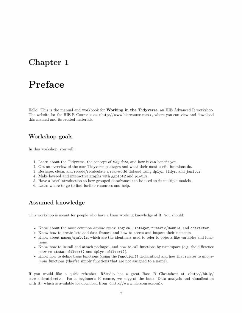
Difference with ‘anti_join()
Use anti_join() when you only want to find rows that don’t occur in both data frames.
anti_join(sw_all, sw_subset, by = c("name", "species")) %>%glimpse()
## Observations: 70## Variables: 3## $ name <chr> "Luke Skywalker", "C-3PO", "R2-D2", "Darth Vader", "...## $ homeworld <chr> "Tatooine", "Tatooine", "Naboo", "Tatooine", "Aldera...## $ species <chr> "Human", "Droid", "Droid", "Human", "Human", "Human"...

48 CHAPTER 8. JOINING DATA FRAMES TOGETHER

Chapter 9
Choosing and renaming columns
In this chapter, we will cover how to select, reorder, and rename the columns of a data frame.
Choosing columns by name
Manual naming
You can choose columns using dplyr::select(). The most basic method of choosing columns is to namethem:
library(tidyverse)
starwars %>%select(name, height, mass) %>%glimpse()
## Observations: 87## Variables: 3## $ name <chr> "Luke Skywalker", "C-3PO", "R2-D2", "Darth Vader", "Lei...## $ height <int> 172, 167, 96, 202, 150, 178, 165, 97, 183, 182, 188, 18...## $ mass <dbl> 77.0, 75.0, 32.0, 136.0, 49.0, 120.0, 75.0, 32.0, 84.0,...
Another method is to name a set of adjacent columns using the : operator, just as you would create a rangeof numbers from 1 to 4 with 1:4:
starwars %>%select(name:mass) %>%glimpse()
## Observations: 87## Variables: 3## $ name <chr> "Luke Skywalker", "C-3PO", "R2-D2", "Darth Vader", "Lei...## $ height <int> 172, 167, 96, 202, 150, 178, 165, 97, 183, 182, 188, 18...## $ mass <dbl> 77.0, 75.0, 32.0, 136.0, 49.0, 120.0, 75.0, 32.0, 84.0,...
49
50 CHAPTER 9. CHOOSING AND RENAMING COLUMNS
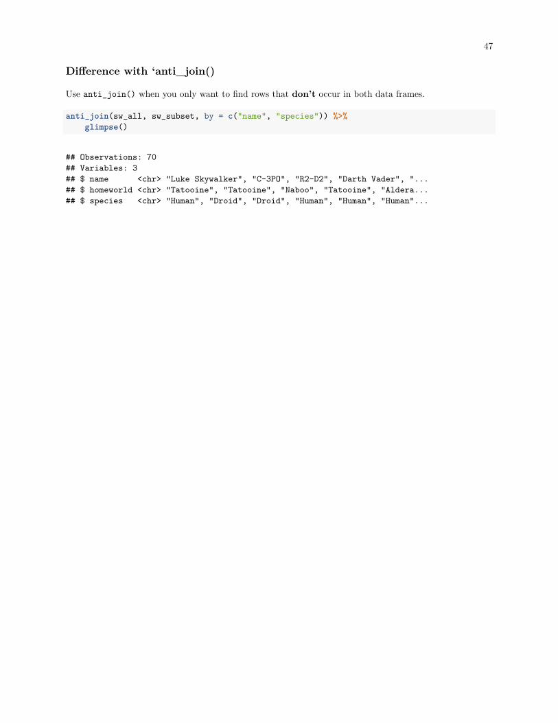
Using a helper function to name
The Tidyverse comes with a set of functions that can be used to programatically select columns by name.They can be viewed in ?tidyselect::select_helpers, but the ones we use most often are:
Helper Chooses column names that. . .starts_with() Start with a literal stringends_with() End with a literal stringcontains() Contains a literal stringmatches() Match a regular expressionnum_range() Are part of a numerical range (x1, x2, . . . )everything() Selects all columns.
For example, we can select all columns from iris that measure Petal, or all columns that measure Length,or any column that has a .:
iris %>%select(starts_with("Petal")) %>%glimpse()
## Observations: 150## Variables: 2## $ Petal.Length <dbl> 1.4, 1.4, 1.3, 1.5, 1.4, 1.7, 1.4, 1.5, 1.4, 1.5,...## $ Petal.Width <dbl> 0.2, 0.2, 0.2, 0.2, 0.2, 0.4, 0.3, 0.2, 0.2, 0.1,...
iris %>%select(ends_with("Length")) %>%glimpse()
## Observations: 150## Variables: 2## $ Sepal.Length <dbl> 5.1, 4.9, 4.7, 4.6, 5.0, 5.4, 4.6, 5.0, 4.4, 4.9,...## $ Petal.Length <dbl> 1.4, 1.4, 1.3, 1.5, 1.4, 1.7, 1.4, 1.5, 1.4, 1.5,...
iris %>%select(contains(".")) %>%glimpse()
## Observations: 150## Variables: 4## $ Sepal.Length <dbl> 5.1, 4.9, 4.7, 4.6, 5.0, 5.4, 4.6, 5.0, 4.4, 4.9,...## $ Sepal.Width <dbl> 3.5, 3.0, 3.2, 3.1, 3.6, 3.9, 3.4, 3.4, 2.9, 3.1,...## $ Petal.Length <dbl> 1.4, 1.4, 1.3, 1.5, 1.4, 1.7, 1.4, 1.5, 1.4, 1.5,...## $ Petal.Width <dbl> 0.2, 0.2, 0.2, 0.2, 0.2, 0.4, 0.3, 0.2, 0.2, 0.1,...
Reordering columns
Columns will be returned in the order they are chosen:

51
iris %>%select(ends_with("Length"), Species, ends_with("Width")) %>%glimpse()
## Observations: 150## Variables: 5## $ Sepal.Length <dbl> 5.1, 4.9, 4.7, 4.6, 5.0, 5.4, 4.6, 5.0, 4.4, 4.9,...## $ Petal.Length <dbl> 1.4, 1.4, 1.3, 1.5, 1.4, 1.7, 1.4, 1.5, 1.4, 1.5,...## $ Species <fct> setosa, setosa, setosa, setosa, setosa, setosa, s...## $ Sepal.Width <dbl> 3.5, 3.0, 3.2, 3.1, 3.6, 3.9, 3.4, 3.4, 2.9, 3.1,...## $ Petal.Width <dbl> 0.2, 0.2, 0.2, 0.2, 0.2, 0.4, 0.3, 0.2, 0.2, 0.1,...
The everything() selector returns every column that isn’t already selected, which makes it useful for re-ordering a data frame’s columns:
iris %>%select(Species, everything()) %>% # Reorder 'Species' to the first columnglimpse()
## Observations: 150## Variables: 5## $ Species <fct> setosa, setosa, setosa, setosa, setosa, setosa, s...## $ Sepal.Length <dbl> 5.1, 4.9, 4.7, 4.6, 5.0, 5.4, 4.6, 5.0, 4.4, 4.9,...## $ Sepal.Width <dbl> 3.5, 3.0, 3.2, 3.1, 3.6, 3.9, 3.4, 3.4, 2.9, 3.1,...## $ Petal.Length <dbl> 1.4, 1.4, 1.3, 1.5, 1.4, 1.7, 1.4, 1.5, 1.4, 1.5,...## $ Petal.Width <dbl> 0.2, 0.2, 0.2, 0.2, 0.2, 0.4, 0.3, 0.2, 0.2, 0.1,...
Omitting columns
With any of the above methods, you can omit a column by putting a - in front of the selection:
iris %>%# Negate the selector to omit its results# ↓select(-Species, -Petal.Length) %>%glimpse()
## Observations: 150## Variables: 3## $ Sepal.Length <dbl> 5.1, 4.9, 4.7, 4.6, 5.0, 5.4, 4.6, 5.0, 4.4, 4.9,...## $ Sepal.Width <dbl> 3.5, 3.0, 3.2, 3.1, 3.6, 3.9, 3.4, 3.4, 2.9, 3.1,...## $ Petal.Width <dbl> 0.2, 0.2, 0.2, 0.2, 0.2, 0.4, 0.3, 0.2, 0.2, 0.1,...
iris %>%select(-ends_with("Length")) %>%glimpse()
## Observations: 150## Variables: 3## $ Sepal.Width <dbl> 3.5, 3.0, 3.2, 3.1, 3.6, 3.9, 3.4, 3.4, 2.9, 3.1, ...## $ Petal.Width <dbl> 0.2, 0.2, 0.2, 0.2, 0.2, 0.4, 0.3, 0.2, 0.2, 0.1, ...## $ Species <fct> setosa, setosa, setosa, setosa, setosa, setosa, se...

52 CHAPTER 9. CHOOSING AND RENAMING COLUMNS
Negating everything() will, of course, return no columns.
Note that because everything() chooses all unselected columns, any omitted columns will be returned. Ifyou use everything(), do your omissions after it:
iris %>%select(Species, everything(), -ends_with("Length")) %>%glimpse()
## Observations: 150## Variables: 3## $ Species <fct> setosa, setosa, setosa, setosa, setosa, setosa, se...## $ Sepal.Width <dbl> 3.5, 3.0, 3.2, 3.1, 3.6, 3.9, 3.4, 3.4, 2.9, 3.1, ...## $ Petal.Width <dbl> 0.2, 0.2, 0.2, 0.2, 0.2, 0.4, 0.3, 0.2, 0.2, 0.1, ...
Choosing columns by value
You can choose columns based on whether they satisfy a logical test by using the special verb select_if().For example, we can choose columns by data type:
starwars %>%select_if(is.numeric) %>% # Using the base R function is.numeric()glimpse()
## Observations: 87## Variables: 3## $ height <int> 172, 167, 96, 202, 150, 178, 165, 97, 183, 182, 188...## $ mass <dbl> 77.0, 75.0, 32.0, 136.0, 49.0, 120.0, 75.0, 32.0, 8...## $ birth_year <dbl> 19.0, 112.0, 33.0, 41.9, 19.0, 52.0, 47.0, NA, 24.0...
Or we can choose columns that meet some arbitrary check by writing our own function that returns TRUEor FALSE:
colSums(iris[1:4])
## Sepal.Length Sepal.Width Petal.Length Petal.Width## 876.5 458.6 563.7 179.9
less_than_500 <- function(x) {sum(x) < 500
}
iris[1:4] %>%select_if(less_than_500) %>%glimpse()
## Observations: 150## Variables: 2## $ Sepal.Width <dbl> 3.5, 3.0, 3.2, 3.1, 3.6, 3.9, 3.4, 3.4, 2.9, 3.1, ...## $ Petal.Width <dbl> 0.2, 0.2, 0.2, 0.2, 0.2, 0.4, 0.3, 0.2, 0.2, 0.1, ...

53
Just as we mentioned in Chapter @ref{the-pipeline}, you can use the tilde (~) as a shortcut to write ananonymous function, so the above could be expressed like this:
iris[1:4] %>%# dot holds the contents of the column being checked# ↓select_if(~ sum(.) < 500) %>%glimpse()
## Observations: 150## Variables: 2## $ Sepal.Width <dbl> 3.5, 3.0, 3.2, 3.1, 3.6, 3.9, 3.4, 3.4, 2.9, 3.1, ...## $ Petal.Width <dbl> 0.2, 0.2, 0.2, 0.2, 0.2, 0.4, 0.3, 0.2, 0.2, 0.1, ...
The select_if() verb is one of several “scoped verbs” that dplyr provides, which we will explore more inthe following chapters.
Renaming columns
In Chapter @ref{reshaping-and-completing} we covered basic column renaming. As a reminder:
library(janitor)
#### Attaching package: 'janitor'
## The following objects are masked from 'package:stats':#### chisq.test, fisher.test
# Standardise names with janitor::clean_names()iris %>%
clean_names() %>%names() # Print the column names
## [1] "sepal_length" "sepal_width" "petal_length" "petal_width"## [5] "species"
# Replace all names with purrr::set_names()iris %>%
set_names("sep_len", "sep_wid", "pet_len", "pet_wid", "spp") %>%names()
## [1] "sep_len" "sep_wid" "pet_len" "pet_wid" "spp"
# Replace some names with dplyr::rename()iris %>%
rename(sep_length = Sepal.Length, sep_width = Sepal.Width) %>%names()
## [1] "sep_length" "sep_width" "Petal.Length" "Petal.Width"## [5] "Species"

54 CHAPTER 9. CHOOSING AND RENAMING COLUMNS

Chapter 10
Choosing rows
In the previous chapter, we look at how to subset a data frame to keep and remove columns. In this chapter,we will learn how to subset a data frame to keep and remove rows, and how to reorder those rows.
Building a dataset with duplicated rows
To illustrate subsetting, we will make a special version of the built-in starwars dataset that contains someduplicated rows:
set.seed(896)
sw_dup <-starwars %>%select(-(films:starships)) %>% # Omit the last 3 columns (they are lists)sample_n(100, replace = TRUE) %>% # replace = TRUE to get duplicate rows.glimpse()
## Observations: 100## Variables: 10## $ name <chr> "Sly Moore", "Mon Mothma", "Finn", "Roos Tarpals", ...## $ height <int> 178, 150, NA, 224, NA, NA, 188, 200, 264, 180, 163,...## $ mass <dbl> 48, NA, NA, 82, NA, NA, NA, 140, NA, 110, 65, 80, 8...## $ hair_color <chr> "none", "auburn", "black", "none", "brown", "none",...## $ skin_color <chr> "pale", "fair", "dark", "grey", "fair", "none", "pa...## $ eye_color <chr> "white", "blue", "dark", "orange", "brown", "black"...## $ birth_year <dbl> NA, 48, NA, NA, NA, NA, NA, 15, NA, NA, NA, NA, 72,...## $ gender <chr> "female", "female", "male", "male", "male", "none",...## $ homeworld <chr> "Umbara", "Chandrila", NA, "Naboo", NA, NA, "Iktotc...## $ species <chr> NA, "Human", "Human", "Gungan", "Human", "Droid", "...
Reordering rows
We’ll also re-order this data frame’s rows using dplyr::arrange() to show that it does indeed containduplicates. Have a look at the result with View(sw_dup).
55

56 CHAPTER 10. CHOOSING ROWS
sw_dup <-sw_dup %>%# Sort rows by homeworld, then species, then name.arrange(homeworld, species, name) %>%glimpse()
## Observations: 100## Variables: 10## $ name <chr> "Bail Prestor Organa", "Leia Organa", "Leia Organa"...## $ height <int> 191, 150, 150, 150, 150, 188, 175, 180, 180, 180, 1...## $ mass <dbl> NA, 49, 49, 49, 49, 79, 79, 110, 110, 110, 82, 82, ...## $ hair_color <chr> "black", "brown", "brown", "brown", "brown", "brown...## $ skin_color <chr> "tan", "light", "light", "light", "light", "light",...## $ eye_color <chr> "brown", "brown", "brown", "brown", "brown", "brown...## $ birth_year <dbl> 67, 19, 19, 19, 19, NA, 37, NA, NA, NA, 92, 92, 92,...## $ gender <chr> "male", "female", "female", "female", "female", "ma...## $ homeworld <chr> "Alderaan", "Alderaan", "Alderaan", "Alderaan", "Al...## $ species <chr> "Human", "Human", "Human", "Human", "Human", "Human...
The default sorting order of arrange() is A-Z for Character columns and in increasing order for Numericand Factor columns. To sort in the opposite direction, use desc():
sw_dup %>%arrange(mass) %>% # Increasing quantity of massglimpse()
## Observations: 100## Variables: 10## $ name <chr> "Yoda", "Yoda", "Wicket Systri Warrick", "Wicket Sy...## $ height <int> 66, 66, 88, 88, 96, 97, 112, 112, 165, 165, 94, 193...## $ mass <dbl> 17.0, 17.0, 20.0, 20.0, 32.0, 32.0, 40.0, 40.0, 45....## $ hair_color <chr> "white", "white", "brown", "brown", NA, NA, "none",...## $ skin_color <chr> "green", "green", "brown", "brown", "white, blue", ...## $ eye_color <chr> "brown", "brown", "brown", "brown", "red", "red", "...## $ birth_year <dbl> 896, 896, 8, 8, 33, NA, NA, NA, 46, 46, NA, NA, NA,...## $ gender <chr> "male", "male", "male", "male", NA, NA, "male", "ma...## $ homeworld <chr> NA, NA, "Endor", "Endor", "Naboo", "Tatooine", "Mal...## $ species <chr> "Yoda's species", "Yoda's species", "Ewok", "Ewok",...
sw_dup %>%arrange(desc(mass)) %>% # Decreasing massglimpse()
## Observations: 100## Variables: 10## $ name <chr> "IG-88", "Tarfful", "Bossk", "Jek Tono Porkins", "J...## $ height <int> 200, 234, 190, 180, 180, 180, 198, 198, 193, 196, 1...## $ mass <dbl> 140, 136, 113, 110, 110, 110, 102, 102, 89, 87, 87,...## $ hair_color <chr> "none", "brown", "none", "brown", "brown", "brown",...## $ skin_color <chr> "metal", "brown", "green", "fair", "fair", "fair", ...## $ eye_color <chr> "red", "blue", "red", "blue", "blue", "blue", "yell...

57
## $ birth_year <dbl> 15, NA, 53, NA, NA, NA, NA, NA, 92, NA, NA, NA, NA,...## $ gender <chr> "none", "male", "male", "male", "male", "male", "ma...## $ homeworld <chr> NA, "Kashyyyk", "Trandosha", "Bestine IV", "Bestine...## $ species <chr> "Droid", "Wookiee", "Trandoshan", "Human", "Human",...
Removing duplicate rows
Use dplyr::distinct() to remove duplicate rows. By default, it will remove a row if every one of its valuesis identical to a previous row’s values (i.e. it keeps the first instance of a duplicated row and discards theother copies).
sw_dup %>%distinct() %>%glimpse() %>%anyDuplicated() # Returns 0 if there are no duplicate rows.
## Observations: 57## Variables: 10## $ name <chr> "Bail Prestor Organa", "Leia Organa", "Raymus Antil...## $ height <int> 191, 150, 188, 175, 180, 198, 196, 150, 180, 170, 1...## $ mass <dbl> NA, 49.0, 79.0, 79.0, 110.0, 82.0, NA, NA, 80.0, 77...## $ hair_color <chr> "black", "brown", "brown", "none", "brown", "white"...## $ skin_color <chr> "tan", "light", "light", "light", "fair", "pale", "...## $ eye_color <chr> "brown", "brown", "brown", "blue", "blue", "yellow"...## $ birth_year <dbl> 67, 19, NA, 37, NA, 92, NA, 48, 29, 21, NA, NA, 54,...## $ gender <chr> "male", "female", "male", "male", "male", "male", "...## $ homeworld <chr> "Alderaan", "Alderaan", "Alderaan", "Bespin", "Best...## $ species <chr> "Human", "Human", "Human", "Human", "Human", "Cerea...
## [1] 0
You can also choose the columns that are compared for duplication. By default it only returns the columnsthat were chosen; to return all of the columns, use the argument .keep_all = TRUE.
sw_dup %>%distinct(species, homeworld) %>% # Only check 'species' and 'homeworld'glimpse() %>%anyDuplicated()
## Observations: 42## Variables: 2## $ species <chr> "Human", "Human", "Human", "Cerean", "Chagrian", "Hu...## $ homeworld <chr> "Alderaan", "Bespin", "Bestine IV", "Cerea", "Champa...
## [1] 0
sw_dup %>%distinct(species, homeworld, .keep_all = TRUE) %>% # Keep all columnsglimpse() %>%anyDuplicated()

58 CHAPTER 10. CHOOSING ROWS
## Observations: 42## Variables: 10## $ name <chr> "Bail Prestor Organa", "Lobot", "Jek Tono Porkins",...## $ height <int> 191, 175, 180, 198, 196, 150, 180, 167, 184, 175, 1...## $ mass <dbl> NA, 79.0, 110.0, 82.0, NA, NA, 80.0, NA, 50.0, 80.0...## $ hair_color <chr> "black", "none", "brown", "white", "none", "auburn"...## $ skin_color <chr> "tan", "light", "fair", "pale", "blue", "fair", "fa...## $ eye_color <chr> "brown", "blue", "blue", "yellow", "blue", "blue", ...## $ birth_year <dbl> 67, 37, NA, 92, NA, 48, 29, NA, NA, 54, 22, 8, NA, ...## $ gender <chr> "male", "male", "male", "male", "male", "female", "...## $ homeworld <chr> "Alderaan", "Bespin", "Bestine IV", "Cerea", "Champ...## $ species <chr> "Human", "Human", "Human", "Cerean", "Chagrian", "H...
## [1] 0
Removing rows with NAs
Use tidyr::drop_na() to remove any row that contains an NA.
sw_dup %>%drop_na() %>%glimpse() %>%anyNA() # Returns FALSE if there are no NAs in the data frame
## Observations: 30## Variables: 10## $ name <chr> "Leia Organa", "Leia Organa", "Leia Organa", "Leia ...## $ height <int> 150, 150, 150, 150, 175, 198, 198, 198, 180, 170, 1...## $ mass <dbl> 49.0, 49.0, 49.0, 49.0, 79.0, 82.0, 82.0, 82.0, 80....## $ hair_color <chr> "brown", "brown", "brown", "brown", "none", "white"...## $ skin_color <chr> "light", "light", "light", "light", "light", "pale"...## $ eye_color <chr> "brown", "brown", "brown", "brown", "blue", "yellow...## $ birth_year <dbl> 19, 19, 19, 19, 37, 92, 92, 92, 29, 21, 21, 54, 54,...## $ gender <chr> "female", "female", "female", "female", "male", "ma...## $ homeworld <chr> "Alderaan", "Alderaan", "Alderaan", "Alderaan", "Be...## $ species <chr> "Human", "Human", "Human", "Human", "Human", "Cerea...
## [1] FALSE
Instead of looking for NAs inside every column, you can choose only some columns. NAs that occur outsidethe chosen columns will be ignored.
sw_dup %>%drop_na(gender:species) %>%glimpse() %>%anyNA() # Returns TRUE because there are still NAs, e.g. in birth_year.
## Observations: 81## Variables: 10## $ name <chr> "Bail Prestor Organa", "Leia Organa", "Leia Organa"...

59
## $ height <int> 191, 150, 150, 150, 150, 188, 175, 180, 180, 180, 1...## $ mass <dbl> NA, 49, 49, 49, 49, 79, 79, 110, 110, 110, 82, 82, ...## $ hair_color <chr> "black", "brown", "brown", "brown", "brown", "brown...## $ skin_color <chr> "tan", "light", "light", "light", "light", "light",...## $ eye_color <chr> "brown", "brown", "brown", "brown", "brown", "brown...## $ birth_year <dbl> 67, 19, 19, 19, 19, NA, 37, NA, NA, NA, 92, 92, 92,...## $ gender <chr> "male", "female", "female", "female", "female", "ma...## $ homeworld <chr> "Alderaan", "Alderaan", "Alderaan", "Alderaan", "Al...## $ species <chr> "Human", "Human", "Human", "Human", "Human", "Human...
## [1] TRUE
Choosing rows by value
One of the most important verbs in dplyr is dplyr::filter(), which is used to subset a data frame toreturn the rows that you’re interested in.
# Find all of the Humans whose homeworld was not Earthsw_dup %>%
# filter() performs an AND search by default.# ↓filter(species == "Human", homeworld != "Earth") %>%distinct() %>%glimpse()
## Observations: 18## Variables: 10## $ name <chr> "Bail Prestor Organa", "Leia Organa", "Raymus Antil...## $ height <int> 191, 150, 188, 175, 180, 150, 180, 170, 167, 188, 1...## $ mass <dbl> NA, 49, 79, 79, 110, NA, 80, 77, NA, 84, NA, 85, 45...## $ hair_color <chr> "black", "brown", "brown", "none", "brown", "auburn...## $ skin_color <chr> "tan", "light", "light", "light", "fair", "fair", "...## $ eye_color <chr> "brown", "brown", "brown", "blue", "blue", "blue", ...## $ birth_year <dbl> 67, 19, NA, 37, NA, 48, 29, 21, NA, 72, NA, NA, 46,...## $ gender <chr> "male", "female", "male", "male", "male", "female",...## $ homeworld <chr> "Alderaan", "Alderaan", "Alderaan", "Bespin", "Best...## $ species <chr> "Human", "Human", "Human", "Human", "Human", "Human...
# Find everyone who is either a Droid OR whose homeworld is Tatooinesw_dup %>%
# OR operator. For more info, read ?base::Logic# ↓filter(species == "Droid" | homeworld == "Tatooine") %>%distinct() %>%glimpse()
## Observations: 7## Variables: 10## $ name <chr> "R2-D2", "R5-D4", "Beru Whitesun lars", "Cliegg Lar...## $ height <int> 96, 97, 165, 183, 163, NA, 200## $ mass <dbl> 32, 32, 75, NA, NA, NA, 140

60 CHAPTER 10. CHOOSING ROWS
## $ hair_color <chr> NA, NA, "brown", "brown", "black", "none", "none"## $ skin_color <chr> "white, blue", "white, red", "light", "fair", "fair...## $ eye_color <chr> "red", "red", "blue", "blue", "brown", "black", "red"## $ birth_year <dbl> 33, NA, 47, 82, 72, NA, 15## $ gender <chr> NA, NA, "female", "male", "female", "none", "none"## $ homeworld <chr> "Naboo", "Tatooine", "Tatooine", "Tatooine", "Tatoo...## $ species <chr> "Droid", "Droid", "Human", "Human", "Human", "Droid...
# Find every human who either has no recorded mass, or is taller than 180 cmsw_dup %>%
filter(species == "Human", (is.na(mass) | height > 180)) %>%distinct() %>%glimpse()
## Observations: 15## Variables: 10## $ name <chr> "Bail Prestor Organa", "Raymus Antilles", "Mon Moth...## $ height <int> 191, 188, 150, 167, 188, 157, 185, 182, 183, 163, N...## $ mass <dbl> NA, 79, NA, NA, 84, NA, 85, 77, NA, NA, NA, NA, NA,...## $ hair_color <chr> "black", "brown", "auburn", "white", "none", "brown...## $ skin_color <chr> "tan", "light", "fair", "fair", "dark", "light", "d...## $ eye_color <chr> "brown", "brown", "blue", "blue", "brown", "brown",...## $ birth_year <dbl> 67, NA, 48, NA, 72, NA, NA, 57, 82, 72, NA, NA, NA,...## $ gender <chr> "male", "male", "female", "female", "male", "female...## $ homeworld <chr> "Alderaan", "Alderaan", "Chandrila", "Coruscant", "...## $ species <chr> "Human", "Human", "Human", "Human", "Human", "Human...
# Find everyone who is 100-170 cm tallsw_dup %>%
filter(between(height, 100, 170)) %>%distinct() %>%glimpse()
## Observations: 14## Variables: 10## $ name <chr> "Leia Organa", "Mon Mothma", "Wedge Antilles", "Joc...## $ height <int> 150, 150, 170, 167, 112, 170, 157, 165, 170, 165, 1...## $ mass <dbl> 49.0, NA, 77.0, NA, 40.0, 56.2, NA, 45.0, 75.0, 75....## $ hair_color <chr> "brown", "auburn", "brown", "white", "none", "black...## $ skin_color <chr> "light", "fair", "fair", "fair", "grey, red", "yell...## $ eye_color <chr> "brown", "blue", "hazel", "blue", "orange", "blue",...## $ birth_year <dbl> 19, 48, 21, NA, NA, 58, NA, 46, 82, 47, 72, NA, NA, NA## $ gender <chr> "female", "female", "male", "female", "male", "fema...## $ homeworld <chr> "Alderaan", "Chandrila", "Corellia", "Coruscant", "...## $ species <chr> "Human", "Human", "Human", "Human", "Dug", "Miriala...

Chapter 11
Editing and creating columns
In this chapter, we will cover how to edit columns in a dataframe and how to calculate new ones.
Mutating columns by name
Creating new columns
The function dplyr::mutate() is used for column creation and editing. Its use is very similar to making anamed vector in base R:
iris %>%mutate(new_column = "recycle_me") %>%glimpse()
## Observations: 150## Variables: 6## $ Sepal.Length <dbl> 5.1, 4.9, 4.7, 4.6, 5.0, 5.4, 4.6, 5.0, 4.4, 4.9,...## $ Sepal.Width <dbl> 3.5, 3.0, 3.2, 3.1, 3.6, 3.9, 3.4, 3.4, 2.9, 3.1,...## $ Petal.Length <dbl> 1.4, 1.4, 1.3, 1.5, 1.4, 1.7, 1.4, 1.5, 1.4, 1.5,...## $ Petal.Width <dbl> 0.2, 0.2, 0.2, 0.2, 0.2, 0.4, 0.3, 0.2, 0.2, 0.1,...## $ Species <fct> setosa, setosa, setosa, setosa, setosa, setosa, s...## $ new_column <chr> "recycle_me", "recycle_me", "recycle_me", "recycl...
If you provide a vector of length 1 as your new column’s contents (as we did above by providing a Charactervector with only 1 element), then mutate() will automatically recycle it. In all other cases, the contents ofthe new column must be as long as the number of rows:
iris %>%# Repeat the names of the months as many times as there are rowsmutate(new_column = rep_len(month.name, length.out = n())) %>%# ↑# n() is the group size -- in an ungrouped data frame it is number of rowsglimpse()
## Observations: 150
61

62 CHAPTER 11. EDITING AND CREATING COLUMNS
## Variables: 6## $ Sepal.Length <dbl> 5.1, 4.9, 4.7, 4.6, 5.0, 5.4, 4.6, 5.0, 4.4, 4.9,...## $ Sepal.Width <dbl> 3.5, 3.0, 3.2, 3.1, 3.6, 3.9, 3.4, 3.4, 2.9, 3.1,...## $ Petal.Length <dbl> 1.4, 1.4, 1.3, 1.5, 1.4, 1.7, 1.4, 1.5, 1.4, 1.5,...## $ Petal.Width <dbl> 0.2, 0.2, 0.2, 0.2, 0.2, 0.4, 0.3, 0.2, 0.2, 0.1,...## $ Species <fct> setosa, setosa, setosa, setosa, setosa, setosa, s...## $ new_column <chr> "January", "February", "March", "April", "May", "...
Calculating with existing columns
To use the data frame’s columns for calculations or logic, just use the columns’ names. dplyr assumes thatyou are referring to columns that are located in the current data frame, so there is no need to refer to thecolumns with $:
iris %>%mutate(add_all = Sepal.Length + Sepal.Width + Petal.Length + Petal.Width) %>%glimpse()
## Observations: 150## Variables: 6## $ Sepal.Length <dbl> 5.1, 4.9, 4.7, 4.6, 5.0, 5.4, 4.6, 5.0, 4.4, 4.9,...## $ Sepal.Width <dbl> 3.5, 3.0, 3.2, 3.1, 3.6, 3.9, 3.4, 3.4, 2.9, 3.1,...## $ Petal.Length <dbl> 1.4, 1.4, 1.3, 1.5, 1.4, 1.7, 1.4, 1.5, 1.4, 1.5,...## $ Petal.Width <dbl> 0.2, 0.2, 0.2, 0.2, 0.2, 0.4, 0.3, 0.2, 0.2, 0.1,...## $ Species <fct> setosa, setosa, setosa, setosa, setosa, setosa, s...## $ add_all <dbl> 10.2, 9.5, 9.4, 9.4, 10.2, 11.4, 9.7, 10.1, 8.9, ...
But be careful! Look at what happens if, instead of manually adding the columns together, we tried to usesum():
iris %>%mutate(sum_all = sum(Sepal.Length, Sepal.Width,
Petal.Length, Petal.Width)) %>%glimpse()
## Observations: 150## Variables: 6## $ Sepal.Length <dbl> 5.1, 4.9, 4.7, 4.6, 5.0, 5.4, 4.6, 5.0, 4.4, 4.9,...## $ Sepal.Width <dbl> 3.5, 3.0, 3.2, 3.1, 3.6, 3.9, 3.4, 3.4, 2.9, 3.1,...## $ Petal.Length <dbl> 1.4, 1.4, 1.3, 1.5, 1.4, 1.7, 1.4, 1.5, 1.4, 1.5,...## $ Petal.Width <dbl> 0.2, 0.2, 0.2, 0.2, 0.2, 0.4, 0.3, 0.2, 0.2, 0.1,...## $ Species <fct> setosa, setosa, setosa, setosa, setosa, setosa, s...## $ sum_all <dbl> 2078.7, 2078.7, 2078.7, 2078.7, 2078.7, 2078.7, 2...
Since sum() operates on entire vectors, it has grabbed the entire contents of the columns and addedthem together, and so the result is always 2078.7 in all rows. You will use this behaviour (calculating bywhole columns) quite often, so it’s something to be mindful of.
Editing an existing column
To edit an existing column, just name it as the target:

63
iris %>%mutate(Species = str_to_upper(Species)) %>%glimpse()
## Observations: 150## Variables: 5## $ Sepal.Length <dbl> 5.1, 4.9, 4.7, 4.6, 5.0, 5.4, 4.6, 5.0, 4.4, 4.9,...## $ Sepal.Width <dbl> 3.5, 3.0, 3.2, 3.1, 3.6, 3.9, 3.4, 3.4, 2.9, 3.1,...## $ Petal.Length <dbl> 1.4, 1.4, 1.3, 1.5, 1.4, 1.7, 1.4, 1.5, 1.4, 1.5,...## $ Petal.Width <dbl> 0.2, 0.2, 0.2, 0.2, 0.2, 0.4, 0.3, 0.2, 0.2, 0.1,...## $ Species <chr> "SETOSA", "SETOSA", "SETOSA", "SETOSA", "SETOSA",...
Mutating multiple columns at a time
You can create and edit many columns together by putting them all in the same mutate() call. Each columnis made one-after-the-other, so you can take the contents of a just-created column and do something elsewith it. For example, let’s do three operations:
1. Find the median length of all petals in iris.2. Flag each observation TRUE if its petal length is longer than the median length, otherwise flag it FALSE.3. Convert TRUE/FALSE into 1/0 by using as.numeric().
set.seed(123)
iris %>%mutate(median_petal_length = median(Petal.Length),
has_long_petals = Petal.Length > median_petal_length,has_long_petals = as.numeric(has_long_petals)) %>%
# Shuffle the rows so you can see both TRUE/1 and FALSE/0 valuessample_frac(size = 1.00) %>%select(Petal.Length, median_petal_length, has_long_petals) %>%head()
## Petal.Length median_petal_length has_long_petals## 1 1.1 4.35 0## 2 1.4 4.35 0## 3 6.7 4.35 1## 4 1.3 4.35 0## 5 5.1 4.35 1## 6 5.2 4.35 1
Programatically choosing columns
In Chapter @ref{choosing-and-renaming-columns} we had the option of using select_if() to choosecolumns based on, say, whether their names contained a particular string. We have the same options in twodifferent versions: mutate_if() and mutate_at().
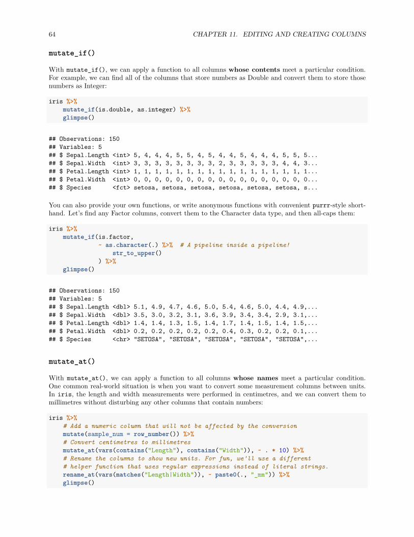
64 CHAPTER 11. EDITING AND CREATING COLUMNS
mutate_if()
With mutate_if(), we can apply a function to all columns whose contents meet a particular condition.For example, we can find all of the columns that store numbers as Double and convert them to store thosenumbers as Integer:
iris %>%mutate_if(is.double, as.integer) %>%glimpse()
## Observations: 150## Variables: 5## $ Sepal.Length <int> 5, 4, 4, 4, 5, 5, 4, 5, 4, 4, 5, 4, 4, 4, 5, 5, 5...## $ Sepal.Width <int> 3, 3, 3, 3, 3, 3, 3, 3, 2, 3, 3, 3, 3, 3, 4, 4, 3...## $ Petal.Length <int> 1, 1, 1, 1, 1, 1, 1, 1, 1, 1, 1, 1, 1, 1, 1, 1, 1...## $ Petal.Width <int> 0, 0, 0, 0, 0, 0, 0, 0, 0, 0, 0, 0, 0, 0, 0, 0, 0...## $ Species <fct> setosa, setosa, setosa, setosa, setosa, setosa, s...
You can also provide your own functions, or write anonymous functions with convenient purrr-style short-hand. Let’s find any Factor columns, convert them to the Character data type, and then all-caps them:
iris %>%mutate_if(is.factor,
~ as.character(.) %>% # A pipeline inside a pipeline!str_to_upper()
) %>%glimpse()
## Observations: 150## Variables: 5## $ Sepal.Length <dbl> 5.1, 4.9, 4.7, 4.6, 5.0, 5.4, 4.6, 5.0, 4.4, 4.9,...## $ Sepal.Width <dbl> 3.5, 3.0, 3.2, 3.1, 3.6, 3.9, 3.4, 3.4, 2.9, 3.1,...## $ Petal.Length <dbl> 1.4, 1.4, 1.3, 1.5, 1.4, 1.7, 1.4, 1.5, 1.4, 1.5,...## $ Petal.Width <dbl> 0.2, 0.2, 0.2, 0.2, 0.2, 0.4, 0.3, 0.2, 0.2, 0.1,...## $ Species <chr> "SETOSA", "SETOSA", "SETOSA", "SETOSA", "SETOSA",...
mutate_at()
With mutate_at(), we can apply a function to all columns whose names meet a particular condition.One common real-world situation is when you want to convert some measurement columns between units.In iris, the length and width measurements were performed in centimetres, and we can convert them tomillimetres without disturbing any other columns that contain numbers:
iris %>%# Add a numeric column that will not be affected by the conversionmutate(sample_num = row_number()) %>%# Convert centimetres to millimetresmutate_at(vars(contains("Length"), contains("Width")), ~ . * 10) %>%# Rename the columns to show new units. For fun, we'll use a different# helper function that uses regular expressions instead of literal strings.rename_at(vars(matches("Length|Width")), ~ paste0(., "_mm")) %>%glimpse()

65
## Observations: 150## Variables: 6## $ Sepal.Length_mm <dbl> 51, 49, 47, 46, 50, 54, 46, 50, 44, 49, 54, 48...## $ Sepal.Width_mm <dbl> 35, 30, 32, 31, 36, 39, 34, 34, 29, 31, 37, 34...## $ Petal.Length_mm <dbl> 14, 14, 13, 15, 14, 17, 14, 15, 14, 15, 15, 16...## $ Petal.Width_mm <dbl> 2, 2, 2, 2, 2, 4, 3, 2, 2, 1, 2, 2, 1, 1, 2, 4...## $ Species <fct> setosa, setosa, setosa, setosa, setosa, setosa...## $ sample_num <int> 1, 2, 3, 4, 5, 6, 7, 8, 9, 10, 11, 12, 13, 14,...
In the above example, we wrapped our ‘select helper’ functions contains() and matches() in anotherfunction called vars(). You don’t need to know much about this function, expect that it allows mutate_at()(and summarise_at(), in the next chapter) to recognise and use these helper functions to pick columns.
Replacing NA values
There are a few functions that let use replace NA values in a column quite effectively. For this demonstration,we will use the built-in dataset starwars because it has a nice mix of NA values.
11.0.1 Replace all NA in a column with one value
If you only want to replace the NAs with the same value, then you can use tidyr::replace_na(). Thisfunction takes a named list of columns where NA should be replaced, and what value it should be replacedwith:
starwars %>%replace_na(list(hair_color = "UNKNOWN",
birth_year = 99999)) %>%glimpse()
## Observations: 87## Variables: 13## $ name <chr> "Luke Skywalker", "C-3PO", "R2-D2", "Darth Vader", ...## $ height <int> 172, 167, 96, 202, 150, 178, 165, 97, 183, 182, 188...## $ mass <dbl> 77.0, 75.0, 32.0, 136.0, 49.0, 120.0, 75.0, 32.0, 8...## $ hair_color <chr> "blond", "UNKNOWN", "UNKNOWN", "none", "brown", "br...## $ skin_color <chr> "fair", "gold", "white, blue", "white", "light", "l...## $ eye_color <chr> "blue", "yellow", "red", "yellow", "brown", "blue",...## $ birth_year <dbl> 19.0, 112.0, 33.0, 41.9, 19.0, 52.0, 47.0, 99999.0,...## $ gender <chr> "male", NA, NA, "male", "female", "male", "female",...## $ homeworld <chr> "Tatooine", "Tatooine", "Naboo", "Tatooine", "Alder...## $ species <chr> "Human", "Droid", "Droid", "Human", "Human", "Human...## $ films <list> [<"Revenge of the Sith", "Return of the Jedi", "Th...## $ vehicles <list> [<"Snowspeeder", "Imperial Speeder Bike">, <>, <>,...## $ starships <list> [<"X-wing", "Imperial shuttle">, <>, <>, "TIE Adva...
Fill NA with the last good row (or next good row)
It’s not strange to meet a table like the one below, where rather than copy-paste the same data acrossmultiple rows, they decided to leave the cells empty instead:

66 CHAPTER 11. EDITING AND CREATING COLUMNS
## # A tibble: 9 x 4## site species sample_num bees_present## <chr> <chr> <dbl> <lgl>## 1 Bilpin A. longifolia 1 TRUE## 2 <NA> <NA> 2 TRUE## 3 <NA> <NA> 3 TRUE## 4 <NA> A. elongata 1 TRUE## 5 <NA> <NA> 2 FALSE## 6 <NA> <NA> 3 TRUE## 7 Grose Vale A. terminalis 1 FALSE## 8 <NA> <NA> 2 FALSE## 9 <NA> <NA> 3 TRUE
You can use tidyr::fill() to fill these kinds of structural NAs. The default behaviour is to fill down,taking the last non-NA value and dragging it into the NA below it:
gap_data %>% # The table above, which this manual built behind-the-scenesfill(site, species) %>%print()
## # A tibble: 9 x 4## site species sample_num bees_present## <chr> <chr> <dbl> <lgl>## 1 Bilpin A. longifolia 1 TRUE## 2 Bilpin A. longifolia 2 TRUE## 3 Bilpin A. longifolia 3 TRUE## 4 Bilpin A. elongata 1 TRUE## 5 Bilpin A. elongata 2 FALSE## 6 Bilpin A. elongata 3 TRUE## 7 Grose Vale A. terminalis 1 FALSE## 8 Grose Vale A. terminalis 2 FALSE## 9 Grose Vale A. terminalis 3 TRUE
Recoding values
You will often want to replace some values in a column. For example, you may want to change the names ofyour sites, or convert words like "yes" and "no" into TRUE and FALSE. There are many ways to do this in R,but we will teach you the two most versatile ones. They are 1) using dplyr::if_else() to choose betweentwo alternatives, and 2) using dplyr::case_when() to choose between multiple alternatives.
if_else()
We can use if_else() to make yes/no decisions about what values in a column to replace. For example,let’s use the built-in dataset warpbreaks and label the wool types, named "A" and "B", with the breed ofsheep the yarn was sheared from:
set.seed(123)
warpbreaks %>%mutate(breed = if_else(wool == "A",
true = "Merino",

67
false = "Corriedale")) %>%sample_frac(size = 1.0) %>% # Shuffle the rows so you can see both labelsglimpse()
## Observations: 54## Variables: 4## $ breaks <dbl> 19, 18, 15, 12, 54, 28, 21, 42, 15, 28, 15, 26, 70, 24...## $ wool <fct> B, A, B, A, A, B, B, B, B, A, A, A, A, B, B, A, B, B, ...## $ tension <fct> L, M, H, M, L, M, M, M, H, H, H, H, L, H, L, L, L, L, ...## $ breed <chr> "Corriedale", "Merino", "Corriedale", "Merino", "Merin...
You may be aware that base R includes a function called ifelse(). The difference between ifelse() anddplyr::if_else() is that if_else() checks that both your true/false cases are the same data type. Thisensures that you always know what your new column’s type is. Here is an example of the base ifelse()doing something unexpected because it does not type-check:
iris %>%# 'check' will be a Double, and TRUE will be silently coerced to '1.0'.# If you used if_else() instead, it would stop you by raising an error.mutate(check = ifelse(Sepal.Length > 5, TRUE, Sepal.Length)) %>%glimpse()
## Observations: 150## Variables: 6## $ Sepal.Length <dbl> 5.1, 4.9, 4.7, 4.6, 5.0, 5.4, 4.6, 5.0, 4.4, 4.9,...## $ Sepal.Width <dbl> 3.5, 3.0, 3.2, 3.1, 3.6, 3.9, 3.4, 3.4, 2.9, 3.1,...## $ Petal.Length <dbl> 1.4, 1.4, 1.3, 1.5, 1.4, 1.7, 1.4, 1.5, 1.4, 1.5,...## $ Petal.Width <dbl> 0.2, 0.2, 0.2, 0.2, 0.2, 0.4, 0.3, 0.2, 0.2, 0.1,...## $ Species <fct> setosa, setosa, setosa, setosa, setosa, setosa, s...## $ check <dbl> 1.0, 4.9, 4.7, 4.6, 5.0, 1.0, 4.6, 5.0, 4.4, 4.9,...
case_when()
To do more complicated replacements with multiple conditions, use case_when(). Think of it as manynested if_else() calls. So instead of the clumsy nested if_else() version:
warpbreaks %>%# Each new if_else() runs if the first check is FALSE# ↓mutate(tension = if_else(tension == "H", true = "High", false =
if_else(tension == "M", true = "Mid", false =if_else(tension == "L",
true = "Low",false = NA_character_)))) %>%
glimpse()
We get the easy-to-read case_when() version:
set.seed(123)
warpbreaks %>%
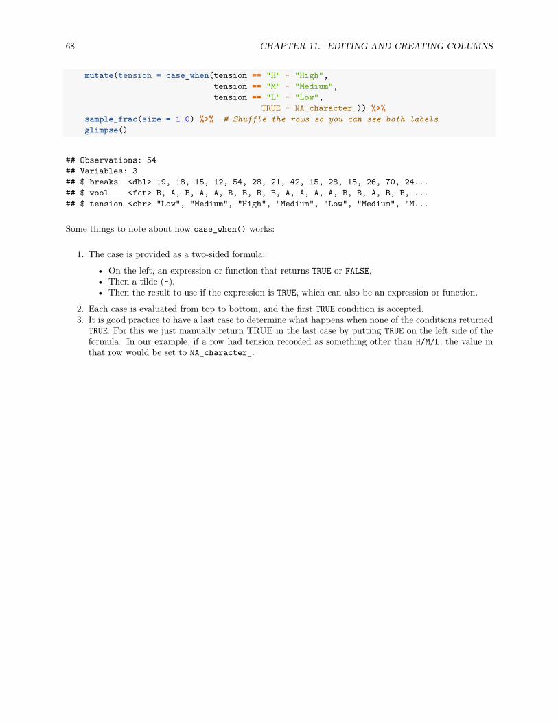
68 CHAPTER 11. EDITING AND CREATING COLUMNS
mutate(tension = case_when(tension == "H" ~ "High",tension == "M" ~ "Medium",tension == "L" ~ "Low",
TRUE ~ NA_character_)) %>%sample_frac(size = 1.0) %>% # Shuffle the rows so you can see both labelsglimpse()
## Observations: 54## Variables: 3## $ breaks <dbl> 19, 18, 15, 12, 54, 28, 21, 42, 15, 28, 15, 26, 70, 24...## $ wool <fct> B, A, B, A, A, B, B, B, B, A, A, A, A, B, B, A, B, B, ...## $ tension <chr> "Low", "Medium", "High", "Medium", "Low", "Medium", "M...
Some things to note about how case_when() works:
1. The case is provided as a two-sided formula:
• On the left, an expression or function that returns TRUE or FALSE,• Then a tilde (~),• Then the result to use if the expression is TRUE, which can also be an expression or function.
2. Each case is evaluated from top to bottom, and the first TRUE condition is accepted.3. It is good practice to have a last case to determine what happens when none of the conditions returned
TRUE. For this we just manually return TRUE in the last case by putting TRUE on the left side of theformula. In our example, if a row had tension recorded as something other than H/M/L, the value inthat row would be set to NA_character_.

Chapter 12
Grouping and summarising
In this chapter, we will cover how to define groups within a data frame (say, grouping the replicates of eachspecies) and how to perform per-group calculations.
An example of groups
Let’s say that we have the built-in dataset storms:
glimpse(storms)
## Observations: 10,010## Variables: 13## $ name <chr> "Amy", "Amy", "Amy", "Amy", "Amy", "Amy", "Amy", "...## $ year <dbl> 1975, 1975, 1975, 1975, 1975, 1975, 1975, 1975, 19...## $ month <dbl> 6, 6, 6, 6, 6, 6, 6, 6, 6, 6, 6, 6, 6, 6, 6, 6, 7,...## $ day <int> 27, 27, 27, 27, 28, 28, 28, 28, 29, 29, 29, 29, 30...## $ hour <dbl> 0, 6, 12, 18, 0, 6, 12, 18, 0, 6, 12, 18, 0, 6, 12...## $ lat <dbl> 27.5, 28.5, 29.5, 30.5, 31.5, 32.4, 33.3, 34.0, 34...## $ long <dbl> -79.0, -79.0, -79.0, -79.0, -78.8, -78.7, -78.0, -...## $ status <chr> "tropical depression", "tropical depression", "tro...## $ category <ord> -1, -1, -1, -1, -1, -1, -1, -1, 0, 0, 0, 0, 0, 0, ...## $ wind <int> 25, 25, 25, 25, 25, 25, 25, 30, 35, 40, 45, 50, 50...## $ pressure <int> 1013, 1013, 1013, 1013, 1012, 1012, 1011, 1006, 10...## $ ts_diameter <dbl> NA, NA, NA, NA, NA, NA, NA, NA, NA, NA, NA, NA, NA...## $ hu_diameter <dbl> NA, NA, NA, NA, NA, NA, NA, NA, NA, NA, NA, NA, NA...
And we want to count the number of hurricanes that were recorded in each month between the years 2005and 2006:
storms %>%filter(status == "hurricane", between(year, 2005, 2006)) %>%distinct(name, year, month) %>%count(year, month) # Counts the number of rows for each year and month
## # A tibble: 8 x 3## year month n
69

70 CHAPTER 12. GROUPING AND SUMMARISING
## <dbl> <dbl> <int>## 1 2005 7 1## 2 2005 8 1## 3 2005 9 5## 4 2005 10 4## 5 2005 12 1## 6 2006 8 1## 7 2006 9 2## 8 2006 10 1
This is the most basic example of what a data frame group is used for. Behind the scenes, thedplyr::count() function is taking storms, grouping its rows by year and month (e.g. “all hurricanes inDecember 2005”), and then counting the number of rows in each group. You can build your own groups todo any calculation in the same way.
Creating your own groups
In a regular ungrouped data frame, operations like dplyr::mutate() are performed across every row — orto put it another way, the entire data frame is a single group, and every row belongs to it.
When a data frame is grouped, those operations are now performed separately within each group. Thinkof it as splitting the data frame into smaller ones, running that operation on each smaller data frame, andthen putting them back together at the end.
Groups are defined using the dplyr::group_by() function. You can look at the groups of a data frame withdplyr::groups(), and dplyr::glimpse() also shows you the groups and how many unique combinationsthere are.
grouped_sw <-starwars %>%group_by(species, homeworld)
groups(grouped_sw)
## [[1]]## species#### [[2]]## homeworld
Ungrouping a data frame
You can remove all groups with dplyr::ungroup(), which you should do when you have finished using them.
grouped_sw %>%ungroup() %>%groups()
## NULL

71
Reducing a grouped data frame
One of the most common reasons for using groups is to summarise a data frame, to combine rows in someway. For these tasks, we use dplyr::summarise():
iris %>%group_by(Species) %>%# summarise() keeps only the grouping columns and the newly-created columns.summarise(avg_pet_len = mean(Petal.Length),
med_pet_len = median(Petal.Length)) %>%glimpse()
## Observations: 3## Variables: 3## $ Species <fct> setosa, versicolor, virginica## $ avg_pet_len <dbl> 1.462, 4.260, 5.552## $ med_pet_len <dbl> 1.50, 4.35, 5.55
This function also comes with scoped variants summarise_at(), summarise_if(), and summarise_all().One of the benefits of summarise_at() is that not only can you choose multiple columns with select helpers,but you can also run multiple functions on those columns by putting them into a list:
iris %>%group_by(Species) %>%summarise_at(vars(ends_with("Length")),
list(~mean(.), ~median(.), ~min(.), ~max(.))) %>%# ↑# A list of anonymous functions, which are also used as column names.glimpse()
## Observations: 3## Variables: 9## $ Species <fct> setosa, versicolor, virginica## $ Sepal.Length_mean <dbl> 5.006, 5.936, 6.588## $ Petal.Length_mean <dbl> 1.462, 4.260, 5.552## $ Sepal.Length_median <dbl> 5.0, 5.9, 6.5## $ Petal.Length_median <dbl> 1.50, 4.35, 5.55## $ Sepal.Length_min <dbl> 4.3, 4.9, 4.9## $ Petal.Length_min <dbl> 1.0, 3.0, 4.5## $ Sepal.Length_max <dbl> 5.8, 7.0, 7.9## $ Petal.Length_max <dbl> 1.9, 5.1, 6.9
starwars %>%group_by(homeworld) %>%# For each homeworld, return the average of any numeric column.summarise_if(is.numeric, ~ mean(., na.rm = TRUE)) %>%drop_na() %>%glimpse()
## Observations: 23## Variables: 4

72 CHAPTER 12. GROUPING AND SUMMARISING
## $ homeworld <chr> "Alderaan", "Bespin", "Cerea", "Concord Dawn", "Cor...## $ height <dbl> 176.3333, 175.0000, 198.0000, 183.0000, 175.0000, 1...## $ mass <dbl> 64.00000, 79.00000, 82.00000, 79.00000, 78.50000, 5...## $ birth_year <dbl> 43.00000, 37.00000, 92.00000, 66.00000, 25.00000, 9...
Groups are dropped with every summary
When you do a summarise() operation, what happens to the groups?
starwars %>%group_by(species, homeworld, hair_color) %>%summarise_if(is.numeric, ~ mean(., na.rm = TRUE)) %>%glimpse()
## Observations: 69## Variables: 6## Groups: species, homeworld [58]## $ species <chr> "Aleena", "Besalisk", "Cerean", "Chagrian", "Clawdi...## $ homeworld <chr> "Aleen Minor", "Ojom", "Cerea", "Champala", "Zolan"...## $ hair_color <chr> "none", "none", "white", "none", "blonde", NA, NA, ...## $ height <dbl> 79.0000, 198.0000, 198.0000, 196.0000, 168.0000, 96...## $ mass <dbl> 15.0, 102.0, 82.0, NaN, 55.0, 32.0, 53.5, 140.0, 40...## $ birth_year <dbl> NaN, NaN, 92.0, NaN, NaN, 33.0, 112.0, 15.0, NaN, 8...
Although we defined 3 groups, only 2 are shown by glimpse(). This is because all the replicate cases ofspecies × homeworld × hair_color have been summarised into a single row each, and so hair_color isno longer meaningful as a grouping variable. If we ever needed to, we could run several summarise() callsin a row, each one progressively ‘rolling-up’ the table until no groups remained.
Reducing an ungrouped data frame
You can also use summarise() on an ungrouped data frame. It will combine every row and drop everythingexcept the new values:
starwars %>%summarise_if(is.numeric, ~ mean(., na.rm = TRUE)) %>%glimpse()
## Observations: 1## Variables: 3## $ height <dbl> 174.358## $ mass <dbl> 97.31186## $ birth_year <dbl> 87.56512
Mutating within groups
If you do not want to remove rows with summarise(), then you can use dplyr::mutate() and its variantsinstead. Remember that for grouped data frames, operations like mutate() are applied separately to eachgroup and not to the entire data frame as a whole. We can illustrate it with the built-in dataset warpbreaks:

73
# Without groups.# Every row of 'breaks' was averaged, so 'avg' is always the same result.warpbreaks %>%
mutate(avg = mean(breaks)) %>%distinct(wool, tension, avg) %>% # Drop rows so that the pattern is obvious.head()
## wool tension avg## 1 A L 28.14815## 2 A M 28.14815## 3 A H 28.14815## 4 B L 28.14815## 5 B M 28.14815## 6 B H 28.14815
# With groups.# 'breaks' was averaged separately for every wool type and tension.warpbreaks %>%
group_by(wool, tension) %>%mutate(avg = mean(breaks)) %>%distinct(wool, tension, avg) %>% # Drop rows so that the pattern is obvious.head()
## # A tibble: 6 x 3## # Groups: wool, tension [6]## wool tension avg## <fct> <fct> <dbl>## 1 A L 44.6## 2 A M 24## 3 A H 24.6## 4 B L 28.2## 5 B M 28.8## 6 B H 18.8

74 CHAPTER 12. GROUPING AND SUMMARISING

Chapter 13
Graphing with ggplot2
In this chapter, we will visit ggplot2 and learn how to build graphs by layering data and graphical elementstogether.
We strongly recommend that you find and use the ggplot2 cheatsheet available at <https://www.rstudio.com/resources/cheatsheets/>. It includes information about many aspects of ggplot2, including previewsof all the geometries available to you and what kinds of input data they need.
The ‘grammar of graphics’
The graphing package ggplot2 is based on a concept of graphics design laid out in a book called TheGrammar of Graphics (Leland Wilkinson et al) and expanded on as the Layered Grammar of Graphics byHadley Wickham.
The short version of these concepts is that a data graphic is built by layering 5 elements:
1. The data set, which has been cleaned and transformed as needed.2. The data points are represented as geometric objects such as circles, squares, or lines.3. These objects are positioned in a coordinate system and scale. For a typical graph, the coordinate
system is Cartesian (X-Y axes on a 2D plane), but the axes themselves (the scales) can be discrete orcontinuous or logarithmic.
4. The geometric objects are modified by mapping data variables to aesthetic properties. For example,points from different groups can be plotted using different colours or shapes.
5. Annotations that label these elements.
Let us build a graphic by layering these elements. We will use the built-in dataset mtcars as the data set:
library(tidyverse)library(ggplot2)
my_dataset <-mtcars %>%# In mtcars, the car model is used as the row name. We don't use row names# in 'tidy' data, so we need to put them into a column.tibble::rownames_to_column("car") %>%mutate_at(vars(car, cyl, vs:carb), as.factor) %>%glimpse()
75

76 CHAPTER 13. GRAPHING WITH GGPLOT2
## Observations: 32## Variables: 12## $ car <fct> Mazda RX4, Mazda RX4 Wag, Datsun 710, Hornet 4 Drive, Hor...## $ mpg <dbl> 21.0, 21.0, 22.8, 21.4, 18.7, 18.1, 14.3, 24.4, 22.8, 19....## $ cyl <fct> 6, 6, 4, 6, 8, 6, 8, 4, 4, 6, 6, 8, 8, 8, 8, 8, 8, 4, 4, ...## $ disp <dbl> 160.0, 160.0, 108.0, 258.0, 360.0, 225.0, 360.0, 146.7, 1...## $ hp <dbl> 110, 110, 93, 110, 175, 105, 245, 62, 95, 123, 123, 180, ...## $ drat <dbl> 3.90, 3.90, 3.85, 3.08, 3.15, 2.76, 3.21, 3.69, 3.92, 3.9...## $ wt <dbl> 2.620, 2.875, 2.320, 3.215, 3.440, 3.460, 3.570, 3.190, 3...## $ qsec <dbl> 16.46, 17.02, 18.61, 19.44, 17.02, 20.22, 15.84, 20.00, 2...## $ vs <fct> 0, 0, 1, 1, 0, 1, 0, 1, 1, 1, 1, 0, 0, 0, 0, 0, 0, 1, 1, ...## $ am <fct> 1, 1, 1, 0, 0, 0, 0, 0, 0, 0, 0, 0, 0, 0, 0, 0, 0, 1, 1, ...## $ gear <fct> 4, 4, 4, 3, 3, 3, 3, 4, 4, 4, 4, 3, 3, 3, 3, 3, 3, 4, 4, ...## $ carb <fct> 4, 4, 1, 1, 2, 1, 4, 2, 2, 4, 4, 3, 3, 3, 4, 4, 4, 1, 2, ...
Now we can layer the graph. Note that ggplot2 has its own pipeline, except that it uses the + operatorinstead of %>% (ggplot2 was written first, so the pipeline concept in R was still being worked out).
my_ggplot <-# 1. Add the data set.
ggplot(data = my_dataset) +# 2. Add the coordinate system and scales.
coord_cartesian() +scale_x_continuous() +scale_y_continuous() +
# 3. Add geometric objects. Here, we add dots to show each data point,# and then add a smoothed line calculated with a linear model.
# 4. Aesthetic properties are mapped in the aes() function. We map the x# position to 'disp', the y position to 'wt', and the colour of the# points to 'cyl'.
geom_point(mapping = aes(x = disp, y = wt, colour = cyl)) +# To change an aesthetic without mapping it to data, set it outside aes().# ↓
geom_smooth(mapping = aes(x = disp, y = wt), linetype = "dashed", method = "lm") +# 5. Add annotations. You can also annotate points in the graph.
labs(x = "Displacement (cubic inches)",y = "Weight (1000 pounds)",title = "Relationship between a car's displacement and weight",subtitle = "Source: Motor Trend US, 1974") +
# A large part of ggplots is that they are very customisable with# themes. We will use this minimal built-in theme.
theme_minimal()
# Print the plotmy_ggplot
A ggplot() call need not be as complicated as this. The package has many sane defaults, such as Cartesiancoordinates and auto-detection of scale types. For example, let’s try a discrete scale on the X axis and acontinuous scale on the Y axis:
ggplot(data = my_dataset, mapping = aes(x = cyl, y = mpg)) +# ↑

77
# Aesthetics in the ggplot() call are used as the defaults for geoms.geom_violin() +geom_jitter(width = 0.025, height = 0, alpha = 0.25) +labs(x = "Number of cylinders",
y = "Miles per gallon",title = "Mileage of cars by cylinder count",subtitle = "Source: Motor Trend US, 1974") +
theme_minimal()
As you can see, layering different geoms together gives you a lot of flexibility in the type of graphic you canmake. The ‘ggplot2 cheatsheet at the start of this chapter shows you the geoms that are available to youand what kinds of data they accept.
Tidy data is incredibly important for ggplot2
Many issues that
Faceting a plot into sub-plots
Sometimes there are many dimensions of data that you would like to present in one plot, and they becomemuddled if they are visualised together:
yarn_plot <-ggplot(warpbreaks, aes(x = breaks, linetype = wool, colour = tension)) +geom_density(aes(y = stat(density)), size = 1) +theme_bw() +theme(legend.position = "top")
yarn_plot
In these cases, it is useful to break the plot into several smaller sub-plots. There are two functions that dothis for you. First, ggplot2::facet_grid() lets you create a regular grid:
yarn_plot +facet_grid(wool ~ tension)
# ↑# Formula interface: Rows ~ Columns.
yarn_plot +facet_grid(. ~ tension)
# ↑# Use 'dot' to mean "no facetting"
If you do not want to create a regular grid, ggplot2::facet_wrap() creates each facet independently andstacks them next to each other to fill the plotting space.

78 CHAPTER 13. GRAPHING WITH GGPLOT2
yarn_plot +facet_wrap(wool ~ tension)
Making plots interactive with plotly
Finally, a great way to explore a new dataset is to make your ggplot interactive by wrapping it inplotly::ggplotly(). This means that you can hover over points and lines to get information about thatdata point, zoom or rescale the axes, and hide or isolate groups. This interactivity can’t be shown in aPDF file, but a document knitted to an HTML page will preserve the interactive components and allow yourcollaborators to explore your graph.
library(plotly)
ggplotly(yarn_plot)

Chapter 14
Modelling
In this chapter, we will cover statistical modelling in the Tidyverse. This chapter will not teach you howto construct or evaluate models, but instead it will focus on how to do those things within the Tidyversephilosophy.
Modelling is generally unchanged
For the most part, you will be using Tidyverse packages to clean, reshape, and summarise your raw databefore feeding the entire dataset into your modelling functions. This means that in general, you will do yourmodelling the same way as you always have:
fitted_model <-iris %>%lm(Sepal.Length ~ Petal.Length, data = .)
plot(Sepal.Length ~ Petal.Length, data = iris)abline(fitted_model, col = "tomato")
The key changes in modelling are that it is now easier to extract model information (with the broom package)and fit models within groups. The package parsnip (still in development) provides a consistent and pipeline-friendly interface for several modelling packages. However, due to time constraints, we leave it to the studentto explore this package if needed.
Extract model data
There are 3 kinds of information that you may want to get out of a fitted model, and so there are threedifferent functions provided by broom to do it. They are:
1. Add model information to an existing data frame with broom::augment().This includes predictions (fitted values), residuals, and standard errors.
2. Create a new data frame of model summary information with broom::glance().These are R-squared, p-value, log-likelihood, AIC and BIC, and others.
3. Create a new data frame of model components with tidy().This is the stuff you would use summary() to look at: variables and their associated estimates, teststatistics, and p-value.
79

80 CHAPTER 14. MODELLING
As an example, we will use the built-in dataset mtcars which contains two columns, disp (cubic inches ofdisplacement, a measure of the car’s volume) and wt (weight in thousands of pounds). Larger cars probablyweigh more, so we will model that:
library(broom)
# Build the modelfitted_model <-
mtcars %>%lm(disp ~ wt, data = .)
# Look at the model's goodness-of-fitfitted_model %>%
glance() %>%glimpse()
## Observations: 1## Variables: 11## $ r.squared <dbl> 0.7885083## $ adj.r.squared <dbl> 0.7814586## $ sigma <dbl> 57.93937## $ statistic <dbl> 111.8496## $ p.value <dbl> 1.22232e-11## $ df <int> 2## $ logLik <dbl> -174.2741## $ AIC <dbl> 354.5482## $ BIC <dbl> 358.9455## $ deviance <dbl> 100709.1## $ df.residual <int> 30
# Look at the model's summaryfitted_model %>%
tidy()
## # A tibble: 2 x 5## term estimate std.error statistic p.value## <chr> <dbl> <dbl> <dbl> <dbl>## 1 (Intercept) -131. 35.7 -3.67 9.33e- 4## 2 wt 112. 10.6 10.6 1.22e-11
# Plot the residualsfitted_model %>%
augment() %>% # Get the fitted values and residualsplot(.resid ~ wt, data = .) # Plot the residuals
broom does not support mixed models. For those, use the package broom.mixed instead.
Running a model within each group
There may be some cases where you would like to run a model separately within each group. Perhaps youwould like to run a model for each site individually, or perhaps you are running a bootstrap analysis withrsample. In these cases, the basic workflow is this:

81
1. Group the data frame with dplyr::group_by() into whatever strata you like.2. Collapse the data frame using tidyr::nest(), which will create a column of data frames, each
holding the raw data for that strata.3. Use dplyr::mutate() and purrr::map() to create a new column that holds the model objects.
Nesting a data frame inside a data frame?
Yes, a data frame (specifically, a tibble, which is the Tidyverse’s modern data frame type) can have acolumn that is typed as a List. In R, a List can hold any object:
tibble(my_list_col = list(1:5, rnorm(10), month.name, iris),strings = c("This", "column", "has", "strings"))
## # A tibble: 4 x 2## my_list_col strings## <list> <chr>## 1 <int [5]> This## 2 <dbl [10]> column## 3 <chr [12]> has## 4 <df[,5] [150 x 5]> strings
The benefit of holding data frames and model objects inside a data frame is that your dataset stays togetherand can be subsetted as a single unit.
14.0.1 An example of nesting and modelling
We’ll use the built-in dataset mtcars again. Imagine that we have data from 32 cars about how far they cantravel on one gallon of fuel (miles per gallon, in the mpg column). We would like to use that information topredict how quickly the car can travel a quarter mile (the qsec column), but we would like to run the modelseparately for cars that have 4, 6, and 8 cylinders (the cyl column). First, we need to nest the data by cyl.
nested_mtcars <-mtcars %>% # In mtcars...group_by(cyl) %>% # Group the data by cylinder count...nest() # And nest the data frames
nested_mtcars
## # A tibble: 3 x 2## cyl data## <dbl> <list>## 1 6 <tibble [7 x 10]>## 2 4 <tibble [11 x 10]>## 3 8 <tibble [14 x 10]>
We now have a data frame with other data frames nested inside them. All of those new data frames areheld in the column data, and they hold all of the rows where cyl == 2, cyl == 4, and cyl == 8. You caninspect them like this:

82 CHAPTER 14. MODELLING
nested_mtcars$data[[2]] %>% # The data for cyl == 4glimpse()
## Observations: 11## Variables: 10## $ mpg <dbl> 22.8, 24.4, 22.8, 32.4, 30.4, 33.9, 21.5, 27.3, 26.0, 30....## $ disp <dbl> 108.0, 146.7, 140.8, 78.7, 75.7, 71.1, 120.1, 79.0, 120.3...## $ hp <dbl> 93, 62, 95, 66, 52, 65, 97, 66, 91, 113, 109## $ drat <dbl> 3.85, 3.69, 3.92, 4.08, 4.93, 4.22, 3.70, 4.08, 4.43, 3.7...## $ wt <dbl> 2.320, 3.190, 3.150, 2.200, 1.615, 1.835, 2.465, 1.935, 2...## $ qsec <dbl> 18.61, 20.00, 22.90, 19.47, 18.52, 19.90, 20.01, 18.90, 1...## $ vs <dbl> 1, 1, 1, 1, 1, 1, 1, 1, 0, 1, 1## $ am <dbl> 1, 0, 0, 1, 1, 1, 0, 1, 1, 1, 1## $ gear <dbl> 4, 4, 4, 4, 4, 4, 3, 4, 5, 5, 4## $ carb <dbl> 1, 2, 2, 1, 2, 1, 1, 1, 2, 2, 2
Now, we must fit the linear models and hold their results in a new column. Since we are creating a newcolumn, we can use dplyr::mutate(). Since we want to iterate over the contents of a column and run afunction on each element, we can use purrr::map():
nested_mtcars <-nested_mtcars %>% # Nested data frames are held in the 'data' column.mutate(model = map(data, # For every df in 'data'...
~ lm(qsec ~ mpg, data = .))) # Fit this model to it.
nested_mtcars
## # A tibble: 3 x 3## cyl data model## <dbl> <list> <list>## 1 6 <tibble [7 x 10]> <lm>## 2 4 <tibble [11 x 10]> <lm>## 3 8 <tibble [14 x 10]> <lm>
We’ve created a new column, model, that holds the lm object that lm() returns. To extract the fitted valuesfrom it, we can run broom::augment() on the model column in the exact same way:
nested_mtcars <-nested_mtcars %>%mutate(fitted = map(model, augment))
nested_mtcars
## # A tibble: 3 x 4## cyl data model fitted## <dbl> <list> <list> <list>## 1 6 <tibble [7 x 10]> <lm> <tibble [7 x 9]>## 2 4 <tibble [11 x 10]> <lm> <tibble [11 x 9]>## 3 8 <tibble [14 x 10]> <lm> <tibble [14 x 9]>
To summarise, we have the groups we set (cyl), the data within each group (data), the linear model thatwas fitted to each group’s data (model), and the fitted values and residuals that were generated by the model(fitted).

83
It time to actually do something with the model information, and we can do that by unnesting the dataframe with tidyr::unnest(). Unnesting will expand the nested data frames into full rows:
modelled_mtcars <-nested_mtcars %>%unnest(fitted) %>% # Expand the data frames in the 'fitted' column.glimpse()
## Observations: 32## Variables: 10## $ cyl <dbl> 6, 6, 6, 6, 6, 6, 6, 4, 4, 4, 4, 4, 4, 4, 4, 4, 4, ...## $ qsec <dbl> 16.46, 17.02, 19.44, 20.22, 18.30, 18.90, 15.50, 18...## $ mpg <dbl> 21.0, 21.0, 21.4, 18.1, 19.2, 17.8, 19.7, 22.8, 24....## $ .fitted <dbl> 17.35903, 17.35903, 17.16235, 18.78491, 18.24406, 1...## $ .se.fit <dbl> 0.8782378, 0.8782378, 1.0180453, 1.0127659, 0.69202...## $ .resid <dbl> -0.89902637, -0.33902637, 2.27764706, 1.43509128, 0...## $ .hat <dbl> 0.26752310, 0.26752310, 0.35947712, 0.35575840, 0.1...## $ .sigma <dbl> 1.824292, 1.888034, 1.256631, 1.674727, 1.898148, 1...## $ .cooksd <dbl> 0.0698916515, 0.0099391078, 0.7882824181, 0.3061425...## $ .std.resid <dbl> -0.61864851, -0.23329478, 1.67605247, 1.05298855, 0...
And now we can do stuff with it, like mutate it further or plot it.
library(ggplot2)
for_plotting <-modelled_mtcars %>%select(cyl:.fitted) %>%gather(data_source, qmile, qsec, .fitted) %>%mutate(data_source =
if_else(data_source == "qsec", "Observed", "Modelled")) %>%glimpse()
## Observations: 64## Variables: 4## $ cyl <dbl> 6, 6, 6, 6, 6, 6, 6, 4, 4, 4, 4, 4, 4, 4, 4, 4, 4,...## $ mpg <dbl> 21.0, 21.0, 21.4, 18.1, 19.2, 17.8, 19.7, 22.8, 24...## $ data_source <chr> "Observed", "Observed", "Observed", "Observed", "O...## $ qmile <dbl> 16.46, 17.02, 19.44, 20.22, 18.30, 18.90, 15.50, 1...
ggplot(data = for_plotting) +geom_point(aes(x = mpg, y = qmile, colour = data_source)) +facet_grid(cyl ~ .) +labs(x = "Miles per gallon", y = "Seconds to travel 1/4 mile") +theme_bw()

84 CHAPTER 14. MODELLING

Chapter 15
Appendix
This document was last compiled on 27 June 2019.
Packages used in this manual
Package Description Version used in this manualtidyverse Installs core Tidyverse packages (partial list below). 1.2.1→ broom Turning model results into data frames. 0.5.1→ dplyr Manipulating, grouping, calculating on data frames. 0.8.1.9000→ forcats Convenience factors for factors. 0.4.0→ ggplot2 Extensible graphing from tidy data. 3.1.0→ haven Convert SPSS/SAS/Stata files to data frames. 2.1.0→ hms Data class for time data. 0.4.2→ lubridate Maths with dates and times. 1.7.4→ magrittr Provides pipes (%>% and others). 1.5→ modelr Modelling inside a pipeline. 0.1.4→ purrr Iteration and functional programming. 0.3.2→ readr Read rectangular data (delimited text files, .CSV, etc.) 1.3.1→ readxl Read data from Excel (.XLS and .XLSX). 1.3.0→ stringr String matching/editing with regular expressions. 1.4.0→ tibble Modern update to base R’s data frames. 2.1.3→ tidyr Reshaping data into tidy format. 0.8.3here Access project-root from anywhere. 0.1janitor Data frame convenience functions. 1.2.0usethis Used to download course materials for this workshop. 1.5.0ViewPipeSteps Show what each pipeline step does to the data. 0.1.0
Datasets used
‘Wood Blocks’ dataset is used with the permission of Jeff Powell and collaborators.‘Insect Light Trap’ dataset is from the University of Copenhagen, in the Public Domain.<https://www.kaggle.com/University-of-Copenhagen/insect-light-trap>‘Mongolia Livestock’ dataset is from Robert Ritz, licensed under CC BY-SA 4.0.<https://www.kaggle.com/robertritz/domesticated-animals-in-mongolia-19702017>
85