No 134- August 2011

Inflation Targeting, Exchange Rate Shocks and Output: Evidence from South Africa

Mthuli Ncube and Eliphas Ndou

Correct citation: Ncube, Mthuli and Ndou, Eliphas (2011), Inflation Targeting, Exchange Rate Shocks and Output: Evidence from South Africa, Working Paper Series N° 134, African Development Bank, Tunis, Tunisia.

Vencatachellum, Désiré (Chair) Anyanwu, John C. Verdier-Chouchane, Audrey Ngaruko, Floribert Faye, Issa Shimeles, Abebe Salami, Adeleke

Coordinator

Working Papers are available online at

http:/www.afdb.org/

Copyright © 2011

African Development Bank

Angle des l’avenue du Ghana et des rues

Pierre de Coubertin et Hédi Nouira

BP 323 -1002 TUNIS Belvédère (Tunisia)

Tél: +216 71 333 511

Fax: +216 71 351 933

E-mail: afdb@afdb.org

Salami, Adeleke

Editorial Committee Rights and Permissions

All rights reserved.

The text and data in this publication may be

reproduced as long as the source is cited.

Reproduction for commercial purposes is

forbidden.

The Working Paper Series (WPS) is produced

by the Development Research Department

of the African Development Bank. The WPS

disseminates the findings of work in progress,

preliminary research results, and development

experience and lessons, to encourage the

exchange of ideas and innovative thinking

among researchers, development

practitioners, policy makers, and donors. The

findings, interpretations, and conclusions

expressed in the Bank’s WPS are entirely

those of the author(s) and do not necessarily

represent the view of the African Development

Bank, its Board of Directors, or the countries

they represent.

Inflation Targeting, Exchange Rate Shocks and 0utput:

Evidence from South Africa

Mthuli Ncube and Eliphas Ndou(1)

_________

AFRICAN DEVELOPMENT BANK GROUP

Working Paper No. 134

August 2011

(1) Mthuli Ncube and Eliphas Ndou are respectively Chief Economist and Vice President of the African Development Bank, Tunis,

Tunisia (M.Ncube@afdb.org) and Researcher at the South African Reserve Bank, Research Department, Pretoria, South Africa.

“This paper will also appear in the Reserve Bank of South Africa research papers"

Office of the Chief Economist

Abstract

This paper derives the inflation equation

to search for a possible transmission

channel between the real interest rate,

inflation rate, exchange rates, real output

growth rate using a Bayesian VAR sign

restriction approach. Our findings show

that the real interest rate reacts

negatively to inflation rate shocks and the

Fisher effect holds in the long run. We

show that strict inflation targeting

approach is not compatible with

significant real output growth. However a

flexible inflation-targeting framework

which attaches a large weight to the role

of real effective exchange rates results in

a significant real output growth given the

Central Bank desire to accumulate more

foreign exchange reserves and high oil

price inflation. Thus real effective

exchange rate measuring competitiveness

against trading partners matters more

than domestic currency and nominal

effective exchange rate depreciations.

JEL Classification: E31, E40, E52, E60

Keywords: Inflation shocks, real interest rate, sign restriction, output growth, inflation-targeting

-5-

1. Introduction

South African monetary policy authorities have in several occasions managed to bring the

inflation rate within the target band of 3-6% after adopting inflation targeting framework in

February 2000. Economic growth in these periods was not significant enough to reduce

unemployment rate. In February 2010, the mandate of the South African Central bank was

clarified with emphasis on taking a balanced approach, which considers economic growth when

monetary policy authorities set interest rates. In the inflation targeting era, the Central Bank has

left the exchange rate to be determined by the market forces making it more volatile. Given this

context, we examine the differences in the responses of real interest rate to the exchange rate

shocks and inflationary shocks, at the same time we examine how these shocks impact on output

growth performance. Moreover we investigate assuming that the Central Bank has desire to

increase reserves accumulation and unexpected high oil prices environment using Bayesian sign

restriction approach.

Inflation targeting is either strict or flexible, depending on the specified loss function of the

central bank. Under strict inflation targeting, the central bank is only concerned about keeping

inflation close to an inflation target over the shorter horizon (Svensson 1997b). This requires

very vigorous activist policies, which involve dramatic interest rate and exchange rate changes.

This happens with considerable variability of exchange rates, interest rates, output, employment

and domestic component of inflation. To some extent the activism probably stabilize inflation

around the inflation target. Flexible inflation targeting occurs when the central bank gives some

weight to the stability of interest rates, exchange rates, output and employment to bring inflation

to the desired long run target over longer horizon. It requires less policy activism which

gradually returns the inflation back to target over a longer horizon. 1Immediately after adopting

inflation targeting approach applying a stricter approach clearly demonstrates the commitment to

the inflation target, builds credibility more quickly, and is more appropriate at the initial phase of

disinflation. However Svensson (1997b) argues that, after the bank has demonstrated

commitment and established credibility to a reasonable degree, there may be more scope for

flexibility without endangering credibility.

Most policy rate reaction functions for Central Banks in an open economy framework have

output gap, inflation gap and exchange rate gap as explanatory variables. Following similar

specification in literature, Granville and Mallick (2010) using monetary policy rule for an open

economy tested empirically the reaction of the interest rate to exchange rate changes and

inflation rate shocks. Estimation incorporated assumptions that the central bank has a desire to

1 Flexible inflation targeting successfully limited not only the variability of inflation but also the variability of the output gap and

the real exchange rate (Svensson 1997b).

-6-

accumulate more reserves even under a negative supply shock in form of higher oil prices. They

imposed sign restrictions to identify exchange rate shocks and inflation shocks to examine

impulse responses functions. They found, using an error correction form and a sign restriction

approach that Russian monetary authorities focused more on targeting the exchange rate rather

than inflation as an instrument for monetary policy.

Firstly, this paper fills the gap in the literature on emerging markets such as South Africa, by

using a Bayesian sign restriction identification system to search the type of monetary policy the

Central bank should adopt to support significant economic growth under flexible inflation

targeting. Secondly, the paper shows that strict inflation targeting approach has a different

growth path compared to the path under flexible inflation targeting framework, in which

significant economic growth could be facilitated through a larger role attached to a particular

exchange rate measure. Thirdly, we also identify the particular measure of exchange rate that is

compatible with significant economic growth. Lastly, we derive the price formation equation and

use the variables in the equation to show that exchange rate can be used to stimulate significant

economic growth.

Recently, there has been great interest in models using large datasets based on factor analysis2

founded on static factors in Bernanke et al (2005) and recently the dynamic factors in Forni and

Gambetti (2010) and large Bayesian models by Banbura (2010). Factor analysis uses more

information, however Forni and Gambetti (2010) exposition suggested that static factors may not

have any economic interpretation and there are often difficulties on the restrictions to be satisfied

by these factors according to theory. However, the above mentioned large datasets

methodologies are not appropriate, based on merits of this study. According to Fry and Pagan

(2007) sign restrictions have provided a useful technique for quantitative analysis, especially

when variables are simultaneously determined, making it harder to justify any parametric

restrictions to resolve the identification problem. However, Scholl and Uhlig (2008) rejected to

embrace Fry and Pagan (2007) argument related to median impulse response in sign restrictions

as an issue arising generally with all identification procedures. Even the latter admits

identifications issues affect all forms of VARs not only those using sign restrictions.

We adopted the sign restriction approach of Granville and Mallick (2010) for this analysis. The

Bayesian sign restriction methodology has advantages over ordinary Vector Autoregresion

(VAR). From a methodological perspective, Fratzscher et al (2010) argues that sign restriction

gives results independent of chosen decomposition of variance–covariance matrix. This implies

that different ordering does not change the result. Furthermore, this method involves a

simultaneous estimation of both reduced-form VAR and the impulse vector. That is, the draws

from the VAR parameters from the unrestricted posterior that do not satisfy the sign restriction,

2 Factor models being parsimonious can model a large amount of information whereas in small VARS the number of variables cannot be

enlarged because of both estimation and identification problems. Bernanke B, Boivin J, Eliasz P (2005) suggested that the natural solution to the

degrees of freedom problem in VAR analyses is to augment standard VARs with estimated factors. Forni and Gambetti (2010) criticised BBE

(2004) identification suggesting this static factors approach through considering factors which are linear combinations of slow-moving variables at the same time excluding fast-moving variables results in an efficiency loss.

-7-

receive a zero prior weight. Granville and Mallick (2010) argue that the sign restriction method

is robust to non-stationarity of series including structural breaks. The advantage is that sign

restriction identification allows shocks to be identified using mild restrictions on multiple time

series. Rafiq and Mallick (2008) suggest restrictions imposed should happen irrespective of how

these inflation, exchange rate variables are measured and their data idiosyncrasies, suggesting

that definitions and measures of same class of variables used are of secondary importance.3

Furthermore, the sign restriction methodology does not put any quantitative restrictions on the

impulse responses. A pure sign restriction approach makes explicit use of restrictions that

researchers use implicitly and are therefore agnostic (Rafiq and Mallick 2008). 4

The sign restrictions adopted from Granville and Mallick (2010), suggests that the oil price does

not decrease as an exogenous positive shock, and the change in foreign exchange reserves

excluding gold does not decrease in response to oil inflation. Inflation does not decline in

response to its own shocks. The paper uses three exchange rates where the positive sign on the

nominal Rand per US dollar implies depreciation of the local currency and the negative sign on

both real and nominal effective exchange rates imply depreciations. The sign restrictions

imposed suggests that the Rand per US Dollar exchange rate will not decline whereas the

nominal and real effective exchange rate should not rise in response to their own shocks.

Moreover, these exchange rates depreciation shocks occur due to own innovations, changes in

foreign exchange reserves and with oil price inflation.

Our findings show that the real interest rate reacts negatively to inflation surprises and is not

significantly different from zero in longer horizons suggesting that the Fisher effect hold in the

long run. The paper showed that strict inflation targeting approach is not compatible with

significant real output growth path. However, we found that under a flexible inflation-targeting

framework, a significant real output growth could be facilitated through a larger role attached to

the real effective exchange rate. The study, concludes that it is a measure of competitiveness

relative to trading partners rather than smoothing the nominal exchange rate volatility levels

which results in significant positive real output growth in the environment of accumulating

reserves and uncertain high oil prices.

We structure the paper such that Section 2 reviews the literature evidence showing that other

variables including the inflation rate matter for the Central Banks. In section 3, we derive the

inflation equation, which shows the relationship amongst variables. Section 4 presents the data,

methodology and describes the sign restriction approach. Sections 5 gives the results from pure

sign restriction approach and summarize the findings from the penalty function. Section 6 gives

the conclusion. The paper has additional graphs in the Appendices.

3 For example the different measures of inflation rate e.g. core inflation and headline inflation. Money measures M3 or M1 or M2 4 As shown in Uhlig (2005) the sign restriction can avoid puzzles by design, for example, price puzzle was avoided by

construction.

-8-

2. Literature review

This section highlights evidence from inflation targeting regimes showing that variables other

than inflation matter for policy makers, especially in the commodity exporting countries.

Inflation targeting is divided into two broad groups, namely strict inflation and flexible inflation

targeting. Strict inflation targeting suggests that the only concern of the central bank is to

stabilize the inflation. It requires vigorous and more active policy changes, involving dramatic

changes in interest and exchange rates. Flexible inflation targeting is when the central bank gives

some weight to the stability of interest rates, exchange rates, output and employment (Svennson

1997b). The policy is conducted in such a manner that the conditional inflation forecast

approaches the inflation target more slowly. The inflation forecast equals the inflation target at a

longer horizon. Evidence showed that flexible inflation targeting successfully limited the

variability of inflation, the variability of the output gap and the real exchange rate. In contrast,

Aghion et al. (2009) showed that exchange rate volatility reduces productivity in developing

countries, attributing it to financial channels. The findings showed the adverse effects of

exchange rate volatility were larger for the less financially developed countries and are

significant for practically all the emerging markets and developing countries.

Recent studies have reviewed whether central banks practice flexible inflation targeting.

Cecchetti and Ehrmann (2000) compared central bank behaviours in 23 industrialised and

developing economies including 9 that target inflation explicitly. They found that inflation

targeters exhibited increasing aversion to inflation variability and decreasing aversion to output

variability. Moreover, they show that inflation targeting countries were able to reduce inflation

volatility at the expense of an increase in output variability. Aghion et al (2009) tested whether

emerging markets follow pure inflation targeting rules or try to stabilize real exchange rates.

Their findings indicated that inflation targeting markets practiced a mixed inflation targeting

strategy. Inflation targeting central banks responded to both inflation and real exchange rates in

setting interest rates. In addition, they find the strongest response to real exchange rate in

countries following inflation targeting policies which are relatively intensive in exporting basic

commodities.

A few studies estimated explicitly the Taylor rule equations for individual countries. Aizenman

et al (2008) suggest that emerging markets which adopted inflation targeting were not following

pure inflation targeting strategies. They found evidence showing that external variables played a

very important role in the Central bank’s policy reaction functions. Central banks respond to real

exchange rate. In addition, inflation targeters with high concentration in commodity exports

change interest rate in a proactive manner in response to real exchange rate than non-commodity

intensive group. Corbo et al (2001) found mixed evidence from seventeen OECD countries

estimated individually. Their results showed that inflation targeters exhibited the largest inflation

coefficients compared to the output gap coefficients. Lubik and Schorfheide (2007) estimated

Taylor type rules in which authorities reacted to output, inflation and exchange rates. The

-9-

findings reveal mixed responses indicating the Australian and New Zealand central banks

changing interest rates in response to exchange rate movements. In contrast the Canadian did not

respond to exchange rates.

De Mello and Moccero (2010) estimated interest rate policy rules for Brazil, Chile, Colombia

and Mexico under the inflation targeting and floating exchange rates in 1999. The interest rate

policy rule was formed in the context of the new Keynesian structural model with inflation,

output and interest rate. Their findings suggest a stronger and persistent response to expected

inflation in Brazil and Chile in the post 1999 inflation targeting period. In Colombia and Mexico

monetary policy has become less counter-cyclical. Minella et al (2003) estimated a reaction

function for the central bank of Brazil, and showed that the coefficient on output gap is not

statistically significant in most of the specifications. Pavasuthipaisit (2010) develops a DSGE

model that also concludes that inflation targeting regimes should respond to the exchange rate

shocks under certain conditions that the paper outlines. Findings from their tests showed that the

policy rule adopted by inflation targeting commodity-intensive developing countries differed

from that of the inflation targeting non-commodity exporter. These finding give support to the

greater sensitivity of commodity inflation targeting countries to exchange rate changes.

We derive the inflation equation and policy reaction rule in context of an open economy in the

next section. We do not estimate both the policy reaction functions and inflation equations in a

univariate setting. Rather we pursue a multivariate approach by estimating the entire structural

model using a Bayesian sign restriction approach with variables from both equations.

3. The inflation equation framework

Before we search for a possible relationship between the real interest rate, inflation rate,

exchange rate, foreign exchange reserves excluding gold growth and output growth (proxied by

growth in manufacturing production) and oil prices, we derive the central bank price formation

equation. The price formation equation is formed in the context of open economy suggesting that

the exchange rate play an important role in decisions affecting demand and supply disturbances.

Thus, we use the variables in the inflation equation and impose restrictions on them, assuming

the inflation equation is followed by the central bank. The central bank has attached less weight

to the role of exchange rate under the strict inflation-targeting framework which is expected to

change under flexible inflation targeting framework.

3.1.Deriving the inflation equation

We adopt the approach of Granville and Mallick (2010) to derive the inflation equation and

reaction function of monetary policy which includes the changes in flow of money (tMS )

decomposed into international reserves (tIR ) and domestic assets (

tDA )

-10-

[1] ttt DAIRMS

Chamberlin (2006) showed that changes in international reserves can be expressed in terms of

the trade balance. However we adjust the equation to take care of the imperfect capital mobility.

[2] )()( tttf

td

tttt eerrKMXIR

The trade balance is given by exports )( tX minus imports )( tM and capital flows )( tK is

determined by the difference between domestic interest rate )( d

tr and foreign interest rate )( f

tr

.5 A trade balance surplus suggests that the Central Bank is adding to reserves accumulation.

)( tt ee refers to the expected change in nominal bilateral exchange rate. An expectation of rand

appreciation against the US dollar would lead to capital inflows. A positive interest differential

which stimulates capital inflows should appreciate domestic currency leading to increased

reserve accumulations. However the net effect of currency appreciation on reserves accumulation

is unclear due to asymmetry effects. Currency appreciation lowers exports and it becomes

cheaper to purchase foreign currency ceteris paribus. The flow of money demand )( tMD for an

open economy function depends on the level of real output )( ty , exchange rate )( te and real

interest rate )( tr . The real interest rate is given by the difference between the nominal interest

rate )( ti and expected inflation )( e

t i.e e

ttt ir . The fisher effect suggests in the long run,

real interest rates should not change because both the nominal interest rate and inflation rate

would have changed by same percentage. We argue that since real interest rate is a linear

combination of two non-stationary variables, it can be stationary in line with other first

differenced variables hence this justifies it being left in levels.

[3] ttttt veryMD and 0,,

These variables have been log-differenced and expressed in percentages and the real interest rate

left in level. Equation [3] shows that transaction demand for nominal balances increases as the

expected inflation levels increases. The expected rate of depreciation in the money demand

function captures the portfolio choice that asset holders face. The exchange rate changes may

increase or reduce the demand for money due to substitution effect or the wealth effect (Hye et al

2009). According to Sriram (2001) the expected depreciation will have a negative effect on

money demand. Thus, an increase in expected depreciation translates into higher expected

returns from holding foreign money hence agents will substitute domestic currency for foreign

5 Balance of payments surplus = increase in official exchange reserves = current account surplus+ net capital inflow. Exports depends on exchange rate and foreign income whereas imports depends upon exchange rate and domestic income. Substituting the bilateral nominal

exchange rate as defined in Blanchard (2006) e

t

f

t

d

tt erre )1()1( suggest a direct negative relationship between high domestic

interest, expected appreciation and lower foreign interest rate hence trade balance will deteriorate.

-11-

currency.6 The effect of interest rate on demand for currency would be negative with an increase

in interest rate and positive for interest bearing demand and time deposits (Kalra 1998).

Conversely, higher real rates of return on alternative assets reduce the incentive to hold money

hence the negative relationship between money and return on alternative assets (Sriram 2001).

Money demand is expected to be positively related to the level of activity. Assuming equilibrium

in the money market holds continuously suggests that ( tt MSMD ). Hence we can write the

capital flow reaction equation as

[4] tttttt IReryDA

The inverse relationship between changes in international reserves and domestic assets implies

that under flexible rate exchange policy, currency changes are likely to influence the conduct of

monetary policy while under fixed exchange rates the bank should sterilize capital inflows to

hold money constant. In equation [4] domestic residents may also hold foreign currency for

transactions or precautionary purposes in the presence of domestic inflation meaning that

domestic currency depreciation may lead to declines in real money balances encouraging

currency substitution (Granville and Mallick 2010). Choudhry (1998) found that the rate of

change in exchange rate should be included in demand equation for M2 to obtain a stationary

long–run relationship. Bahmani-oskooee (1991) included the effective exchange rate measure in

the money demand equation.

The aggregate inflation ( t ) supply equation can be formulated on the basis of an open economy

Phillips curve, as done in Granville and Mallick (2010)

[5] tttttt DAey 0

Domestic assets term suggests that if the currency does not change in response to changes in

capital inflows, then an increase in money growth can contribute to generating inflation ( t ). We

also include the oil price ( 0

t ) in order take into account the external oil price shocks as a source

of inflation pressures. Therefore substituting equation [4] into equation [5] gives

[6] )()()( 0

tttttttt IRery

The equation suggests inflation should go down as real interest rate increases; should rise as

currency depreciates; and inflation can be reduced when international reserves increase by

allowing currency to appreciate flowing capital inflows when the central bank does not sterilize

the capital inflows. The negative effect of international reserves accumulation can be neutralised

6 Kalra (998) suggest that a- priori the sign on expected depreciation in indeterminate and depends on whether broad money is defined to include

or exclude foreign currency denominated deposits The inclusion of broad money is defined to include foreign currency deposits. Therefore an

expected depreciation in the exchange rate could induce a migration into foreign currency denominated assets hence the shift in the composition

of broad money towards foreign currency denominated assets implying coefficients on exchange rate is positive. In contrast a shift to foreign currency contributing negative component to exchange rate changes .

-12-

by currency depreciation. The dominance of the latter over reserves accumulation can lead to

inflation. The monetary policy authorities determine the interest rates, increasing it to lower

inflation rate via monetary contraction and giving little weight to exchange rates hence

establishing a trade off between the exchange rate and inflation. For an open economy, the

Taylor rule can be written for the unobservable equilibrium real interest rate to include exchange

rates

[7] tttt eyr *)(

The parameters , and give the size of the response of monetary policy measured by

interest rate to output, inflation gap and changes from exchange rates. The interpretation of the

reaction function suggests that real interest rate is increasing in the excess of inflation rate over

the inflation target, in current output and exchange rate depreciation. Growth in money declines

in equation [3] as real interest rates increase, hence stabilising inflation rate in Phillips equation.

Granville and Mallick (2010) suggest that Fisher effect holds when the real interest rate should

not change in response to changes in inflation. Alternatively the inflation rate can have one to

one positive effect on the nominal interest rate. Also the exchange rate depreciations can produce

an increase in real interest rate and their simultaneous inclusion will therefore disentangle their

effects on the real interest rate .

This paper derives the aggregate supply equation which is formulated following the open

economy Phillips curve. This formulation defines the inflation rate in terms of foreign exchange

reserves, oil price shocks, real interest rate, exchange rate and output. The focus of this analysis

differs from the research aim done by Granville and Mallick (2010). We impose restrictions on

the identified variables in the aggregate supply equation for a different purpose to that of

Granville and Mallick (2010). The paper assesses which policy shocks between different

exchange rate shocks and inflation rate shocks can achieve positive real output growth rates

given variables in the inflation equation in South Africa and the central bank maintenance of

price stability remaining essentially.

4. Bayesian VAR model and identification

4.1. VAR model

We estimate the inflation shocks and three exchange rate depreciation shocks in South Africa in

the framework of VAR. The sign identification starts with the estimation of a reduced-form VAR

equation [9]. For simplicity we omitted the intercept term and dummies.

[8] ttt uBYY 1

Where tY is an 1n vector of data series at date Tt ,....,2,1 where B=[B1, B2, ….Bp] is the

vector of matrix of lagged coefficients and tu is the one-step ahead prediction error and the

-13-

variance-covariance matrix is . Assuming independence of fundamental innovations, we need

to find matrix A which satisfies tt Au . The jth

column of A, that is j represents the

immediate impact on the variables of the jth

fundamental shock equivalent to one standard

deviation in size on the n-endogenous variables in the system. Hence the variance–covariance is

given by AAAAEuuE tttt )()( . To identify A, we need at least n(n-1)/2 restrictions

on A . The reduced form disturbance are orthogonalised by Cholseky decomposition, which use

recursive structure on A making it lower triangular matrix.

4.1.2 Pure sign restriction

We adopt the Bayesian sign restriction approach (see Uhlig (2005) Mountford and Uhlig (2009),

Fratzscher et al (2010)) to identify the VAR model through imposing sign restrictions on the

impulse responses of a set of variables. The identification here searches over the space of

possible impulse vectors i

iA to find those impulses responses which agree with the sign

restrictions. The aim is to find impulse vector a where nRa , given that there is an n-

dimensional vector q of unit length so that qAa~

where AA~~ and A

~ is a lower triangular

Cholesky factor of .

The first part of section 5 reports results of individual identified fundamental shocks. We show

that the impulse responses for n-variables up to horizon S can be calculated for a given impulse

vector ja , after estimating coefficients in B using the ordinary least squares. The unique

impulse response function is given by equation [8] as done in Fratzscher et al (2010)

[9] js aBr 1]1[

The sr denotes the matrix of impulse responses at horizon S . Sign restrictions are imposed on a

subset of the n variables over horizon S,...,1,0 such that the impulse vector ja identifies the

particular shock of interest. The estimation of impulse responses is obtained by simulation.

Given the estimated reduced form VAR, we draw q vectors from the uniform distribution in nR

divided it by its length to obtain a candidate draw for ja and calculate its impulse responses

while discarding any q where the sign restrictions are violated. The estimation and inferences is

done as explained below. In the sign restriction approach a prior is formed for the reduced form

VAR model. Using the Normal-Wishart in ),( B as the prior implies the posterior is the

Normal-Wishart for ),( B times the indicator function on Ãq. The indicator function separate

draws which satisfied the sign restriction from those which fail to do so. A joint draw from the

posterior of the Normal-Wishart for ),( B and draws from the unit sphere are drawn from

posterior distribution to get a candidate q vectors. We use the draws from the posterior to

calculate the Cholskey decomposition as important computational tool rather than shocks

identification tool. From each q draw we compute the associated aj vectors and impulses

responses and these impulses are subject to further selection. For those impulse responses which

-14-

satisfy the sign restrictions the joint draws on ),,( aB are stored otherwise they are discarded.

The error bands are calculated from draws kept from 1000 draws which satisfy the sign

restrictions. As such, this first part focuses on estimation of one shock.

The second part of section 5 report the impulse responses of two identified fundamental shocks,

that is, 2k . The above approach is extended to include two shocks. As such, we characterize

the impulse matrix ],[ )2()1( aa as of rank 2 rather than all of A in robustness test. We impose the

restrictions based on economic prior’s expectations on the impulse responses together with

restrictions that ensure orthogonality of the fundamental shocks. By construction the covariance

between fundamental shocks tt)2()1( , corresponding to )2()1( ,aa is zero meaning that these

fundamental shocks are orthogonal.

Hence any impulse matrix ]...[ )()1( kaa can be written as product QAqaa k ~]...[ )()1( of the lower

triangular Cholesky factor A~

of with k x n matrix ]...[ )()1( kqqQ of orthonormal rows )( jq

such that kIQQ . This is a consequence of noting that AA~~ 1 must be an orthonormal matrix

for any decomposition AA~~

of . Denoting )(saa where ns ,....2,1 represents a

column of the impulse matrix. We also denote )(1)( ~ ss qAqq as the corresponding column of

Q . Therefore the impulse responses for the impulse vector a can be written as a linear

combination of the impulse responses to the Cholesky decomposition of in a way described

below. Denoting )(srji to be the impulse response of the

thj variable at horizon s to the thi

column of A~

, and the n-dimensional column vector ],...,[)( 1 niii rrkr . The n-dimensional

impulse response asr at horizon s of impulse vector )(sa is given by

[10]

n

i

isias rqr1

where iq is the ith

entry of )(sqq . We identify )1(a , )2(a using the appropriate sign restrictions

)1()1( ~qAa and )2()2( ~

qAa at the same time jointly impose orthogonality conditions in the

form 0)1( qq and 0)2( qq . In general a joint draw is taken from the posterior of the Normal-

Wishart for ),( B to obtain the candidate q vectors. Each draw for q that satisfy the above

restrictions is kept otherwise it is discarded. The error bands are calculated from draws stored

from 10000 draws which satisfy the sign restrictions. Pure sign restriction approach makes

explicit use of restrictions that researchers use implicitly and are therefore agnostic.

We use the penalty function approach to test the robustness of the results from both single

shocks. Moreover we replace reserves excluding gold with foreign exchange. The penalty

function developed by Uhlig (2005) rewards responses that are consistent with the restrictions

-15-

and penalizes heavily those violating the restrictions. Unlike the pure sign restriction approach,

the penalty function uses additional restrictions which lead to possible distortion of the true

direction of the responses from the imposed sign restrictions. We use pure sign restrictions in

main body of the paper and penalty function approach in robustness analysis.

4 .2. The empirical model

We adopted Granville and Mallick (2010) sign restriction identification approach which is robust

to both non-stationarity of the series including breaks. The exchange rate and inflation rate

shocks effects are restricted to last at least K=6 months. We argue that the monetary policy

authorities reaction to these variables has implications on the output stabilisation outcomes.

Strict inflation targeting does not attach any weight to output gap stabilisation. The instrument is

set such that conditional inflation forecast equals the inflation target. Any shocks causing

deviations between the conditional inflation forecast and the inflation target are met by an

instrument adjustment that eliminates the deviation. In contrast, flexible inflation targeting

attaches a positive weight on output gap stabilisation, interest rate, real exchange rate and

inflation. The policy instrument under flexible inflation targeting is adjusted such that

conditional inflation forecast approaches the long run inflation gradually, minimising

fluctuations on output gap, exchange rate and interest rates. The larger the weight attached on

output gap stabilization, the slower the adjustment of conditional inflation forecast towards the

long run inflation target.

The role of exchange rate in an open economy framework is important in the monetary

transmission mechanism. Real exchange rates affect aggregate demand channel of the monetary

transmission of monetary policy. It affects the relative prices between domestic and foreign

goods and foreign demand for domestic goods. The direct exchange rate channel for monetary

policy transmission, affects inflation through domestic price of imported goods and intermediate

inputs, which are components of consumer price inflation. In addition, it affects nominal wages

via the effect on inflation on wage setting, the foreign demand for domestic goods which impact

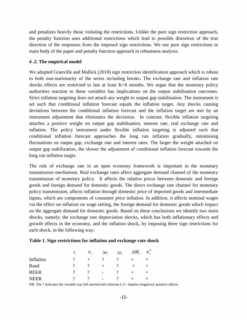
on the aggregate demand for domestic goods. Based on these conclusions we identify two main

shocks, namely; the exchange rate depreciation shocks, which has both inflationary effects and

growth effects in the economy, and the inflation shock, by imposing three sign restrictions for

each shock, in the following way:

Table 1. Sign restrictions for inflation and exchange rate shock

tr t

te ty

tIR 0

t

Inflation ? + ? ? + +

Rand ? ? + ? + +

REER ? ? - ? + +

NEER ? ? - ? + + NB. The ? indicates the variable was left unrestricted whereas (-)/+ implies (negative)/ positive effects

-16-

Firstly, the sign restrictions imposed suggest that, the oil price does not decrease as an exogenous

positive shock. Secondly, the change in foreign exchange reserves does not decrease in response

to oil inflation or exchange rate depreciations. The study uses three exchange rates. The positive

sign on the Rand price of one dollar implies depreciation of the rand. However, the negative sign

on both the real effective exchange rate and nominal effective exchange rate imply depreciation.

Thirdly, the rand per dollar exchange rate change will not decline in response to its own positive

shock whereas both nominal and real effective exchange rates should not rise after depreciation

shock. We assume these exchange rate depreciations should occur due to own innovations and

changes in reserves and oil price inflation.

The overall inflation does not decline in response to its own shock. South African foreign

exchange reserves excluding gold accumulation increased since the adoption of the inflation-

targeting framework. Therefore, a monetary or inflation shock can emerge from changes in

reserves growth or due to oil price inflationary shock. Domestic currency depreciation makes

domestic exports cheaper relative to imported goods and can lead to rising inflation rates. Higher

demand for domestic goods partly due to increased export demand can increase industrial

production. However we refrain from prejudging this outcome and let impulse responses reveal

it. Moreover, exchange rate changes can be either an appreciation or depreciation depending on

the direction of change. These asymmetric outcomes are equally likely under the pure sign

restriction. However, this method keeps those impulse vectors which satisfy the imposed sign

restriction while discarding those violating them in response to a unit shock innovation.

4. The Data

The study uses monthly data from January 2000 to January 2010 under the inflation-targeting

regime.7 We use six variables namely, the growth in foreign exchange reserves excluding gold,

output growth approximated by manufacturing production growth, inflation rate, growth in

nominal rand, nominal effective exchange rate (NEER), real effective exchange rate (REER),

growth in oil price index and real interest rate. We use data extracted from the International

Monetary Fund IFS database. We use three measures of exchange rate namely, the nominal rand

per US dollar (R/$), NEER and REER in separate estimations. The real interest rate equals the

difference between nominal interest rate and expected inflation rate. We calculate the expected

inflation rate using the methodology in Davidson and Mackinnon (1985).8 Both the inflation rate

and expected inflation rate display similar trends in figure A1 in Appendix A. We calculated the

7 The percentage calculated using the year on year percentage changes approach alters the starting period. The estimation period starts from

January 2001 rather 2000 . However we need the observation from 2000. 8 We adopted Davidson and Mackinnon (1985) method. The procedure first calculated the weighted inflation rate using this following equation.

Weighted inflation 4321 .03.03.02.0 tttt

w

t . Then regress inflation (t ) on the constant,

weighted inflation rate (w

t ) and trend. The forecast inflation rate from the regression becomes the expected inflation. The real interest rate

)( tr is given by difference between nominal interest rate )( ti and expected inflation (e

t ) i.e e

ttt ir

-17-

growth rates as year on year percentage changes.9 A positive increase in REER and NEER

represents appreciation respectively and domestic currency depreciation.

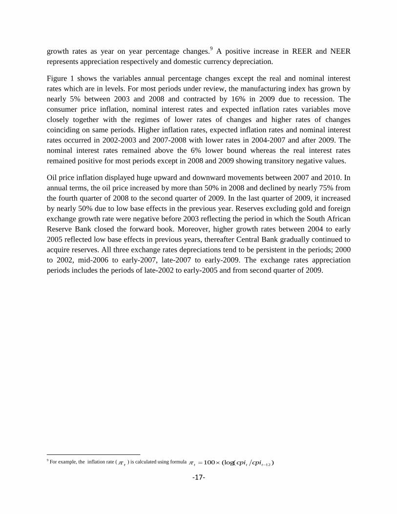
Figure 1 shows the variables annual percentage changes except the real and nominal interest

rates which are in levels. For most periods under review, the manufacturing index has grown by

nearly 5% between 2003 and 2008 and contracted by 16% in 2009 due to recession. The

consumer price inflation, nominal interest rates and expected inflation rates variables move

closely together with the regimes of lower rates of changes and higher rates of changes

coinciding on same periods. Higher inflation rates, expected inflation rates and nominal interest

rates occurred in 2002-2003 and 2007-2008 with lower rates in 2004-2007 and after 2009. The

nominal interest rates remained above the 6% lower bound whereas the real interest rates

remained positive for most periods except in 2008 and 2009 showing transitory negative values.

Oil price inflation displayed huge upward and downward movements between 2007 and 2010. In

annual terms, the oil price increased by more than 50% in 2008 and declined by nearly 75% from

the fourth quarter of 2008 to the second quarter of 2009. In the last quarter of 2009, it increased

by nearly 50% due to low base effects in the previous year. Reserves excluding gold and foreign

exchange growth rate were negative before 2003 reflecting the period in which the South African

Reserve Bank closed the forward book. Moreover, higher growth rates between 2004 to early

2005 reflected low base effects in previous years, thereafter Central Bank gradually continued to

acquire reserves. All three exchange rates depreciations tend to be persistent in the periods; 2000

to 2002, mid-2006 to early-2007, late-2007 to early-2009. The exchange rates appreciation

periods includes the periods of late-2002 to early-2005 and from second quarter of 2009.

9 For example, the inflation rate (

t ) is calculated using formula )(log(100 12 ttt cpicpi

-18-

Figure 1. Plot of variables

Table 2 shows the descriptive statistics of all variables, in particular the mean, standard

deviation, minimum and maximum values. Oil price inflation has the highest standard deviation

value indicating that it is the most volatile variable with both the minimum and maximum

growth rate exceeding 65%. All the three exchange rate measures show that the exchange rates

deviate from their means by 15-21%, which is higher than deviations of both inflation, expected

inflation and interest rates. The reserves excluding gold as well as foreign exchange show

deviations from the mean growth rates of about 20%. These percentage deviations from both

reserves and foreign exchange mean growth rates exceed percentage deviation of CPI inflation

rate, nominal interest rate, real interest rates and expected inflation rate. In terms of mean growth

rates reserves excluding gold and foreign exchange experienced average growth rates of at least

18% which are the highest growth rates compared to all other variables possible indicating the

active accumulation of both reserves and foreign exchange by the Reserve Bank. The growth in

manufacturing volume index is extremely low and being less than 1% over the period and its

deviation from the mean is nearly 7 possible reflecting huge negative effect of the recession in

2009.

Changes in Manufacturing index (%)

2001 2002 2003 2004 2005 2006 2007 2008 2009-25

-15

-5

5

Consumer price level inflation (%)

2001 2002 2003 2004 2005 2006 2007 2008 20090.0

2.5

5.0

7.5

10.0

12.5

Oil price inflation (%)

2001 2002 2003 2004 2005 2006 2007 2008 2009-100

-50

0

50

Changes in Total Reserves minus Gold (%)

2001 2002 2003 2004 2005 2006 2007 2008 2009-10

10

30

50

70

Changes in Foreign Exchange (%)

2001 2002 2003 2004 2005 2006 2007 2008 2009-10

10

30

50

70

Changes in Rand-dollar (%)

2001 2002 2003 2004 2005 2006 2007 2008 2009-50

-25

0

25

50

Nominal interest rate (%)

2000 2001 2002 2003 2004 2005 2006 2007 2008 20096

8

10

12

Changes in NEER (%)

2001 2002 2003 2004 2005 2006 2007 2008 2009-40

-20

0

20

Changes in REER (%)

2001 2002 2003 2004 2005 2006 2007 2008 2009-40

-20

0

20

40

Real Interest Rate (%)

2000 2001 2002 2003 2004 2005 2006 2007 2008 2009-1

1

3

5

7

Expected Inflation Rate (%)

2000 2001 2002 2003 2004 2005 2006 2007 2008 20090

4

8

12

-19-

Table 2. Descriptive statistics

Variable Mean Std Error Minimum Maximum

Nominal interest rate 9.01 1.90 6.43 12.8

CPI inflation rate 5.99 3.13 0.16 12.2

Oil price index inflation rate 8.94 35.0 -80.8 65.7

Rand 1.55 20.6 -42.0 47.1

NEER 3.98 16.5 -37.7 28.8

REER 0.23 15.7 -34.7 31.1

Manufacturing Index 0.89 6.43 -22.5 8.90

Reserves excluding gold 18.4 20.2 -7.13 72.4

Foreign exchange 18.4 21.0 -7.27 75.0

Real Interest rate 2.75 1.73 -0.95 6.43

Expected inflation rate 6.24 2.95 0.89 12.6

NB. All the variables excluding Nominal interest rate, expected inflation rate and real interest

rate are percentages in levels. The remaining variables represent percentage growth rates.

6. Results

We compare the effects of exchange rate depreciation shocks to those of inflation shocks on how

they influence real output growth rates using VAR sign restriction approach with 6 lags. We

restrict shock effects to last at least K=6 months (see Uhlig (2005); Mallick and Rafiq (2008)).

The stabilization of output, employment or the real exchange rate is a reason for hitting the

inflation target at a longer horizon under flexible inflation targeting (Svensson 1997).

Furthermore, the variability of the output, employment and real exchange rate and not their

average levels are important. Hence this framework involves less policy activism and the gradual

returning of the inflation rate back to the target rate which reduces the variability of output,

employment and real exchange rate. The first part of the analysis presents results based on

individual estimation of shocks following the Uhlig (2005) approach. The second part discuses

the results based on Mountford and Uhlig (2009) approach which takes orthogonal property

between fundamental shocks and impulse responses when two shocks are estimated together. We

also perform three robustness tests using the penalty function, changing the horizon period in

which shocks are expected to last from K=6 months to K=9 months and using foreign exchange

amount rather than total reserves excluding gold. We use growth in nominal exchange rate

denoting nominal rand per US dollar changes. We approximate real output by manufacturing

output since it contributed 18% to country’s GDP.

-20-

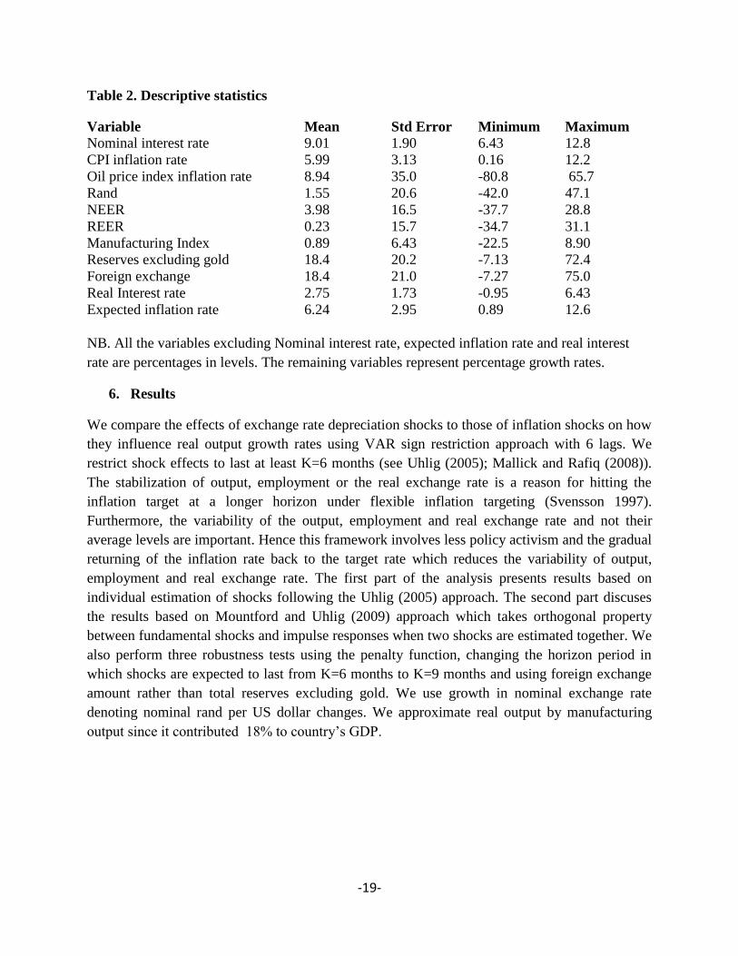
Figure 2. Exchange rate shocks

NB growth in nominal exchange rate refers to rand per US dollar changes

-21-

Figure 2 shows the responses to the nominal rand per US dollar, nominal effective exchange rate

and real effective exchange rate depreciation shocks respectively. Consistent with economic

theoretical predictions, inflation responds positively to currency depreciation across all measures

of exchange rates. These three different exchange rates depreciations significantly increase

inflation rate by a maximum of 0.8 percentage points in the seventh month. After 19 months, the

inflation increase converges to 0.4 percentage points which is not significantly different from

zero. Foreign reserves growth remains positive for 10 months exceeding the imposed six months

(i.e. shock duration). Granville and Mallick (2010) suggest that high foreign exchange reserves

and high real interest rates should appreciate domestic currency. However, we do not find

significant evidence of the Rand appreciation in the long run.

All three exchange rates depreciations have a positive impact on output growth but this is

significant for 8 months under the REER depreciation only. We suggest the volatile currency

which fails to self-correct resulting in persistent appreciations in certain periods as in figure 1,

under inflation targeting may weaken output growth. Moreover, we notice that the manufacturing

growth and oil price inflation weakened in the long run. This could be due to delayed exchange

rate appreciations after a depreciation which erodes the manufacturing competitiveness whereas

persistent inflation pressures had negative effects on real output as suggested by Friedman

(1977). It is plausible for oil price inflation to decline in long-run despite South Africa being a

small open economy which cannot influence world prices. Mishkin (2007) argues that in the long

run the country which becomes more productive relative to other countries expects its currency

to appreciate. Oil price inflation should decline following such domestic currency appreciation.

-22-

The impulse responses between output and reserves show close co-movements. Concurrent

declines in reserves and manufacturing could be explained using equation [2] indicating that

reserves accumulation is also driven by developments in manufactured exports. Thus

depreciation which stimulates growth in manufactured output improves the accumulated foreign

reserves. Moreover, foreign reserve accumulation could result from physical accumulation of

reserves and monthly revaluations. Persistent exchange rate appreciations or depreciation alter

the amount of reserves in any point in time during revaluation process. The lack of significant

evidence of currency appreciation suggests the dominance of manufacturing exports over

exchange rate effects in influencing reserve accumulation.

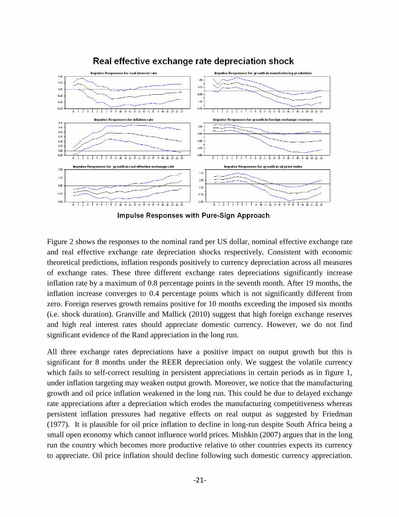
The inflation dynamics in response to an inflation shock are less persistent compared to those

arising from exchange rate shocks. Granville and Mallick (2010) argue that the New Keynesian

theoretical models do not predict a sufficient degree of inflation persistence after a monetary

shock. They suggest that inflation should rise and recede to zero quickly rather than dying slowly

as predicted by empirical literature. In addition, inflation rises for some extended periods in

response to an exchange rate depreciation and the increase is not significant after 18 months

under the NEER and REER depreciation while it remains persistently so under nominal rand

depreciation.

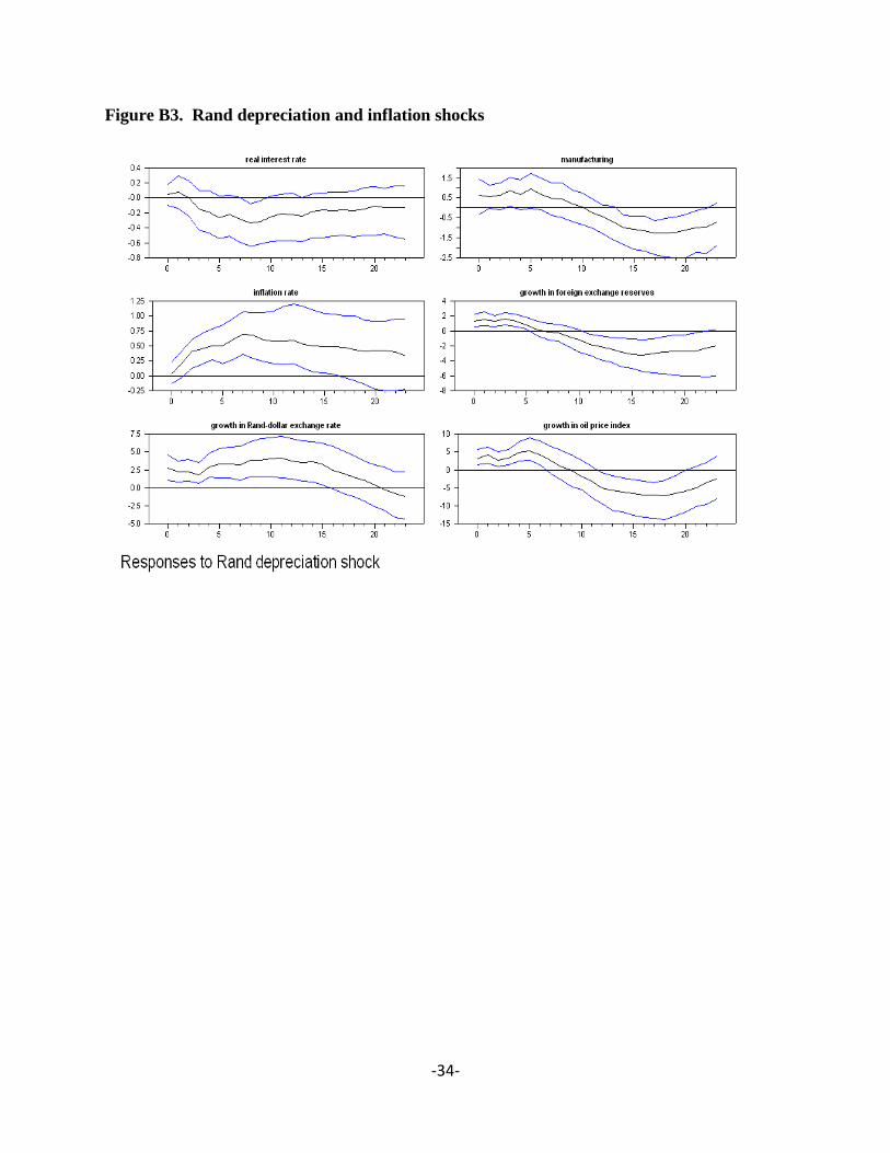
Figure 3: Inflation shocks

-23-

In figure 3, the real interest rates fall significantly and retreat to pre-shock levels. This suggests

that with a change in inflation rate, the nominal interest rate is changing marginally less than the

change in inflation. Monetary policy conducted in forward looking manner, requires interest

rates smoothing over time in anticipation that inflation would eventually fall within the target

band. In long run, the Fisher effect holds as the change in real interest rate is not significantly

different from zero. This implies that the nominal interest rate increased by the similar change in

inflation rate. We conclude that monetary policy is effective in controlling inflation over the long

horizon.

Growth in manufacturing output remains significantly positive for long periods in response to

REER depreciation relative to both rand and nominal effective exchange rate depreciations.

Furthermore, similar to the rand and nominal effective exchange rate, the results suggest that real

effective exchange rate depreciation contribute to inflationary pressures. However, the Central

Bank increases interest rate to lower the inflation rate in the long run. This indicates that policies

which hugely affect the pricing behaviour to depreciate real effective exchange rate aimed to

improve competitiveness, have positive real effects on output growth.

6.1.1 Results from estimating two shocks using orthogonality assumption

We assess the impacts of the exchange rate and inflation shocks under the orthogonality

assumption to avoid sequential estimation and ordering problems. Rafiq and Mallick (2008)

argued that sequentially estimation procedure may lead to sampling problems suggesting the

sequence of shocks would affect the results. Hence, we draw the two vectors simultaneously to

eliminate any sampling uncertainty created by such sequentially sampling draws. Furthermore,

the order in which the shocks are established can have implications for the final results. Our

structural shocks are orthogonally drawn and impulse vectors subsequently derived which makes

the ordering of these shocks less important for the results. These results are robust to changes in

the order of the two shocks.

-24-

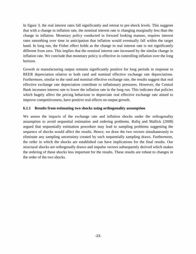
Figure 4. Comparison of exchange rate depreciation shocks and inflation shocks

Figure 4 shows the paired effects of shocks on manufacturing for comparative purposes.

Moreover all impulse responses are presented in Appendix B. These results do not differ from

those estimated using individual shocks. Similarly, the inflationary shocks have an insignificant

stimulus on manufacturing growth. In contrary, the real effective exchange rate leads to

significant growth in manufacturing for at least 7 months whereas the rand-dollar and nominal

effective exchange rates have no such effects on manufacturing output growth rate. Thus the

previous conclusions are robust to the orthogonality and robust to ordering suggesting these

impulse responses do not contain sampling uncertainty created by sequentially ordering of the

shocks.

-25-

6.1.2. Variance decomposition analysis

Table 3. Variance decomposition of all exchange rate shocks and inflation shocks on

manufacturing growth

Steps NEER RAND REER INFNEER INFRAND INFREER

1 8.7% 8.9% 10.7% 8.8% 8.7% 8.6%

2 11.0% 10.9% 12.7% 10.9% 11.3% 10.1%

3 12.5% 12.4% 13.6% 11.9% 11.8% 12.1%

4 12.6% 12.5% 14.0% 12.0% 12.1% 12.6%

5 13.2% 13.2% 14.3% 12.5% 12.4% 13.0%

6 13.4% 13.3% 14.8% 12.4% 12.6% 13.2%

7 13.7% 13.4% 14.9% 12.5% 12.9% 13.4%

8 13.6% 13.5% 15.0% 12.6% 13.4% 13.5%

9 13.9% 13.8% 15.2% 12.6% 13.5% 13.6%

10 14.2% 14.1% 15.3% 12.7% 13.6% 13.7%

11 14.4% 14.3% 15.3% 13.0% 13.7% 14.0%

12 14.5% 14.7% 15.5% 13.2% 13.8% 14.2%

13 14.9% 15.1% 15.6% 13.3% 14.3% 14.3%

14 15.0% 15.2% 15.6% 13.6% 14.5% 14.5%

15 15.0% 15.7% 15.4% 13.8% 14.7% 14.7%

16 15.2% 15.7% 15.4% 13.9% 14.8% 14.8%

17 15.4% 15.9% 15.4% 14.0% 14.9% 15.0%

18 15.6% 15.9% 15.5% 14.2% 14.9% 15.1%

19 15.8% 16.0% 15.6% 14.5% 14.9% 15.2%

20 16.1% 16.0% 15.7% 14.6% 15.0% 15.1%

21 16.2% 15.9% 15.7% 14.7% 15.1% 15.2%

22 16.3% 15.9% 15.8% 14.8% 15.2% 15.2%

23 16.5% 16.0% 15.7% 14.8% 15.2% 15.2%

24 16.5% 16.0% 15.7% 14.8% 15.2% 15.4% NB Inflneer, inflrand and inflreer refers to inflation shocks estimated using nominal effective exchange rate (NEER), rand dollar

exchange rate and real effective exchange rate (REER). Steps ahead refers to horizons in months.

Table 3 shows the variance decompositions of different exchange rate shocks and the various

inflation shocks estimated under three exchange rates. The variance explained by inflation

shocks is lower than the corresponding variability explained by exchange rate shocks over all

horizons. Amongst these three exchange rates, real effective exchange rate (REER) induces more

variability in manufactured output in 14 months relative to rand exchange rates and 17 months

relative to NEER. Moreover, the REER long run values are lower than other exchange rate long

run values.

6.1.3 Robustness analysis

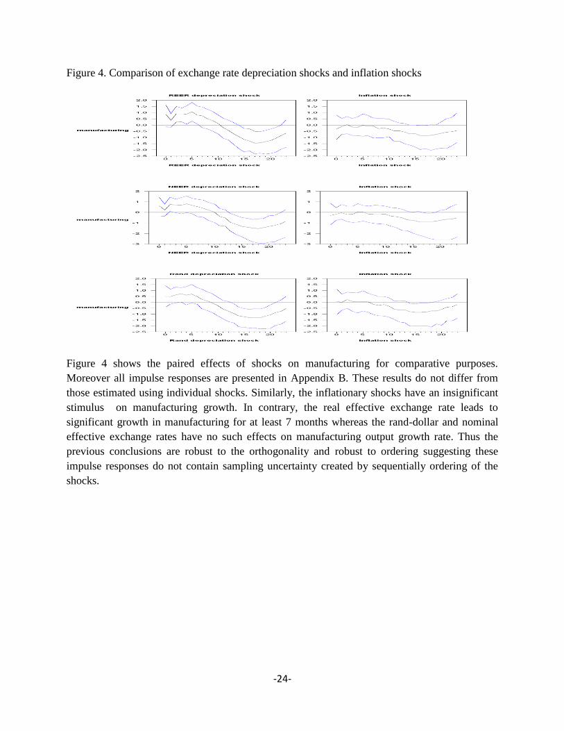
This section examines robustness of the earlier findings using penalty function, changing

horizons for which shocks are expected to last and using foreign exchange under orthogonality

assumptions. Figure 5 shows manufacturing impulse responses from the penalty function

-26-

confirming the findings from pure sign restriction approach. However we report all impulses

responses from the penalty function in Appendix C. The error bands from the penalty functions

look qualitatively similar to pure impulse responses; however these magnitudes are larger with

error bands considerably much sharper. The penalty function searches for large initial reaction of

exchange rate and inflation shock separately. The additional restrictions imposed in the penalty

function introduce some distortion in pure sign restriction results. The findings suggest that the

real effective exchange rate depreciation outperforms the nominal rand depreciation and nominal

effective exchange rate depreciation under the same constraints by achieving higher growth

rates. Output grew by nearly 1%, which is larger than growth rates achieved under both nominal

rand and nominal effective exchange rates shocks. Under the inflation shocks, no significant

output growth rates are achieved under same constraints. These findings are therefore robust.

Figure 5 All exchange rate depreciation shocks and inflation shocks from penalty function

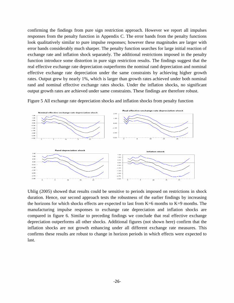
Uhlig (2005) showed that results could be sensitive to periods imposed on restrictions in shock

duration. Hence, our second approach tests the robustness of the earlier findings by increasing

the horizons for which shocks effects are expected to last from K=6 months to K=9 months. The

manufacturing impulse responses to exchange rate depreciation and inflation shocks are

compared in figure 6. Similar to preceding findings we conclude that real effective exchange

depreciation outperforms all other shocks. Additional figures (not shown here) confirm that the

inflation shocks are not growth enhancing under all different exchange rate measures. This

confirms these results are robust to change in horizon periods in which effects were expected to

last.

-27-

Figure 6. Effects of exchange rate and inflation shocks on manufacturing for K=9 months

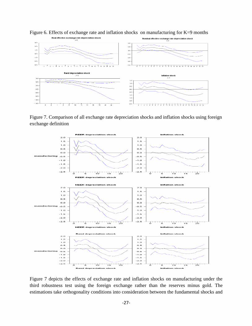
Figure 7. Comparison of all exchange rate depreciation shocks and inflation shocks using foreign

exchange definition

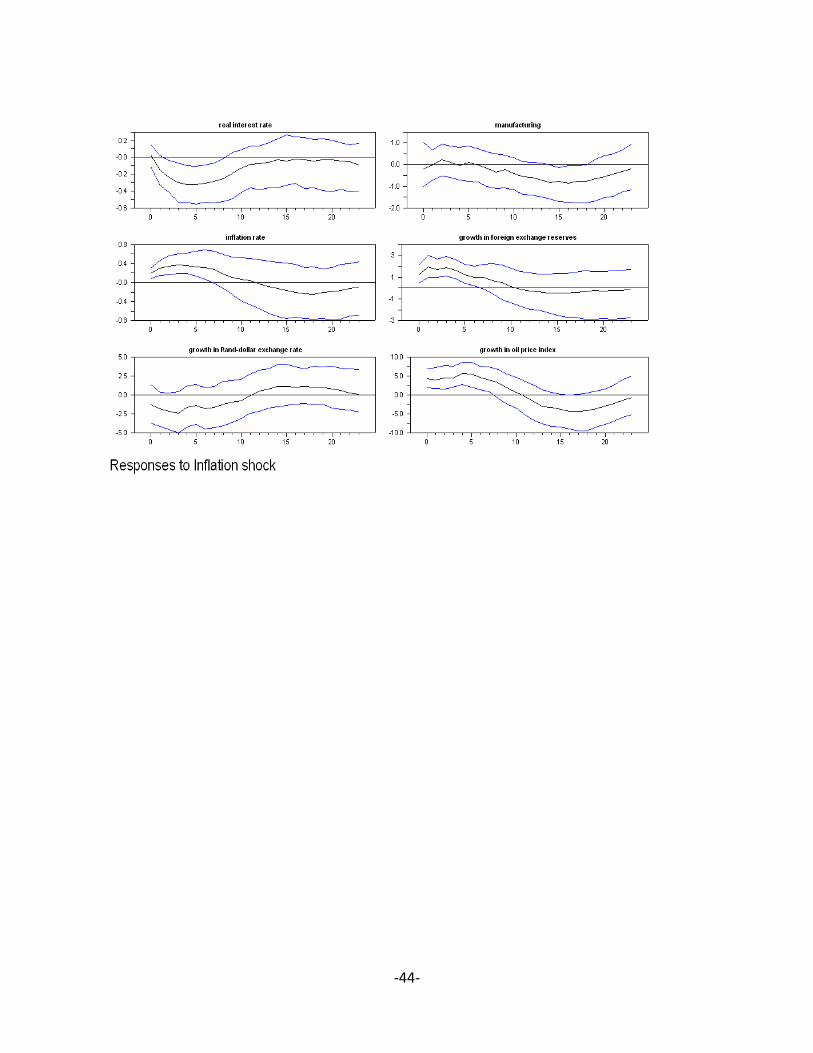
Figure 7 depicts the effects of exchange rate and inflation shocks on manufacturing under the

third robustness test using the foreign exchange rather than the reserves minus gold. The

estimations take orthogonality conditions into consideration between the fundamental shocks and

-28-

impulse responses of two shocks. The full results are attached in the Appendix D. Similarly, the

real effective exchange rate (REER) depreciation leads to significant manufacturing growth

compared to the rand-dollar and nominal effective exchange rate. Moreover, we reach the same

conclusion (results not shown here) using the foreign exchange when shocks are assessed

individually. Overall, the findings in this paper suggest the results are robust to change in

definition of reserves and orthogonality assumption.

7. Conclusion

This paper investigates the relationship between real interest rate, inflation and exchange rate

shocks in an environment of foreign reserves accumulation and oil price inflation, in South

African inflation-targeting regime. We find significant evidence showing that the real interest

rate reacts negatively to the inflation rate shocks. However this reaction is not significantly

different from zero in longer horizon suggesting that the Fisher effect holds in the long run. This

indicates both the nominal interest rate and inflation rate have increased by nearly the same

magnitudes confirming the effectiveness of monetary policy in the long run to both shocks.

Evidence from inflation shocks suggest that the monetary policy authorities’ loss function paid

more attention to bringing inflation towards the inflation target and less or no weight attached on

output stabilisation. Thus strict inflation targeting approach is not compatible with significant

real output growth. In contrast, we find that the REER depreciation has significant growth

enhancing ability relative to other shocks. The inflationary effects from exchange rate

depreciations are significantly dampened through monetary policy tightening. We find that under

the flexible inflation targeting framework giving more weight to the real effective exchange rate

results in significant real output growth. In policy terms, this implies focusing more on the

exchange rate which deals with competitiveness relative to trading partners in an environment of

reserves accumulation and uncertain high oil prices. Even under such circumstances monetary

policy manage to control the inflation pressures associated with such a shock.

References

Aghion, P., Bacchetta, P., Ranciere, R., Rogoff, K. (2009). “Exchange rate volatility and

productivity growth: The role of financial development”. Journal of monetary Economics, 56

(4), 494-513

Aizenman, J., Hutchison, M., Noy, I. (2008). “Inflation targeting and real exchange rate rates in

emerging markets”. NBER working paper 14561

Banbura M, Giannone D, Reichlin L. (2010). “Large Bayesian vector” Journal of Applied

Econometrics 25: 71-92

Bernanke B, Boivin J, Eliasz P. (2005). “Measuring monetary policy: a factor augmented

autoregressive (FAVAR) approach”. Quarterly Journal of Economics 120: 387.422.

-29-

Bahmani-Oskooee , M., (1991), “The demand for money in an open economy: The united

kingdom”, Applied economics , vol 23, pp , 1037-1042

Cecchetti, S., Ehrmann, M.M (2000). “Does inflation targeting the output volatility? An

international comparison of policy makers` preferences and outcomes”. Central Bank of Chile

working papers, no 69,

Chamberlin, G., Yeuh , L. (2006) Macroeconomics ,Thompson learning

Corbo, V., Landerretche, O., Schimdt-Hebbel, K. (2001) . “Assessing inflation targeting after a

decade of world experience”. International Journal of Finance and Economics, 6, 343-368.

De Mello, L., Moccero, D.(2010). “Monetary policy and macroeconomic stability in Latin

America: The cases of Brazil, Chile, Colombia and Mexico Journal of International Money and

Finance xxx , 1-17

Fratzscher, M., Juvenal, L., Sarno, L., (2010). “Asset prices, exchange rates and the current

account.” European economic review , 54 , 643-658

Friedman, M. (1977) . Nobel lecture : Inflation and unemployment. Journl of political Economy,

85, 452-472

Fry, R.A., Pagan, A.R., (2007). Some issues in using sign restrictions for identifying structural

VARs. National Center for Economic Research Working Paper 14.

Granville, B., Mallick, S., (2010), “Monetary policy in Russia: Identifying exchange rate

shocks”, Economic Modelling, 27 , 432-444

Kalra, S., (1998), “Inflation and money demand in Albania”, IMF working paper WP/98/101.

Lubik, T. and F. Schorfheide. (2006 ). “A Bayesian Look at New Open Economy

Macroeconomics.” In NBER Macroeconomics Annual 2005, edited by M. Gertler and K. Rogoff.

MIT Press.

Lubik, T. and F. Schorfheide.(2007). “Do Central Banks Respond to Exchange Rate

Movements? A Structural Investigation.” Journal of Monetary Economics 54(4): 1069–87.

Minella. Andre., Paulo Springer de Freitas, Illan Goldfajn, Marcelo Kfoury Muinhos (2003).

“Inflation targeting in Brazil: Constructing credibility under exchange rate volatility”. Journal of

International Money and Finance, 22 (7), December 1015-1040

Mishkin, F.S., (2007). The economics of Money, Banking and Financial Markets, eighth edition,

Pearson Education Inc

Mountford, A., Uhlig, H., (2009), "What are the Effects of Fiscal Policy Shocks?", Journal of

Applied Econometrics.

-30-

Pavasuthipaisit, R. (2010). “Should inflation-targeting central banks respond to exchange rate

movements? ” Journal of international money and finance , 29 460-485

Rafiq ,M.S., S.K. Mallick. (2008). The effect of monetary policy on output in EMU3. A sign

restriction approach. Journal of Macroeconomics 30 1756–1791

Davidson, R., Mackinnon, J,G., (1985), “Testing linear and log-linear regressions against the

Box-Cox Alternatives”, Canadian Journal of Economics, Vol.18, pp. 499-517

Scholl, A., Uhlig, H., (2008) “New evidence on the puzzles: Results from agnostic identification

on monetary policy and exchange rates”. Journal of International Economics 76 , 1–13

Sriram , S, S., (2001), “ A survey of recent empirical money demand studies” IMF staff papers ,

vol. 47, no 3

Svensson, Lars E.O. (1997a), . “Inflation Targeting: Some Extensions”,. NBER Working

Paper No. 5962.

Svensson, Lars E.O. (1997b). “Inflation Targeting in an Open Economy: Strict vs. Flexible

Inflation Targeting ”. Public Lecture held at Victoria University of Wellington, November

Svensson Lars E.O. (2000), “Open economy inflation targeting”, Journal of International

economics, vol 50, pp 155-183

Uhlig, H. (2005). “What are the effects of monetary policy on output? Results from an agnostic

identification Procedure” . Journal of monetary economics 52, 381- 419

Appendix A

Figure A1: Inflation and Inflation expectation graph

-31-

Appendix B . Results from orthogonality assumption

Figure B1. NEER depreciation and inflation shocks

-32-

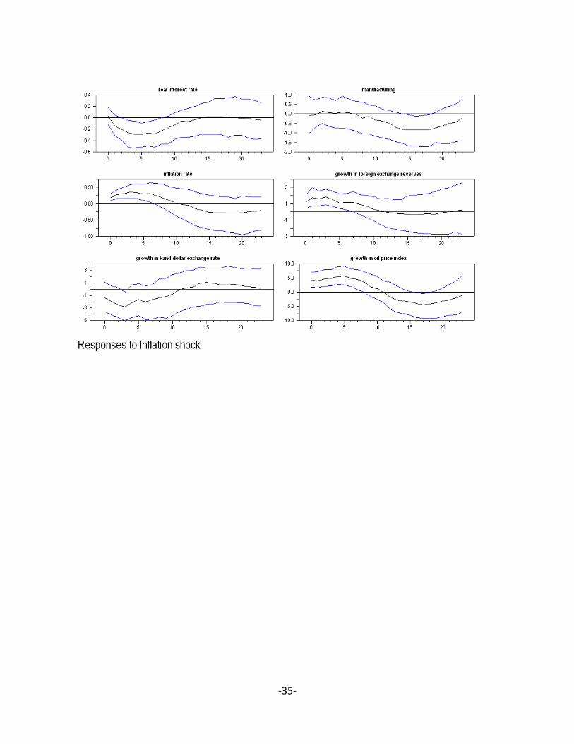
Figure B2. REER depreciation and inflation shocks

-33-

-34-

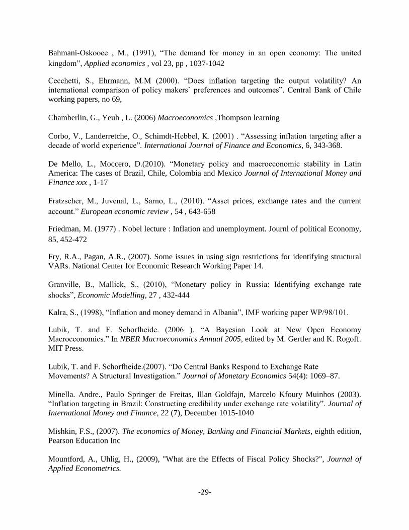
Figure B3. Rand depreciation and inflation shocks

-35-

-36-

Appendix C : Sensitivity results using penalty function

Figure C1: Exchange rate shocks (Penalty function)

-37-

Figure C2. Inflation shocks (Penalty function)

-38-

-39-

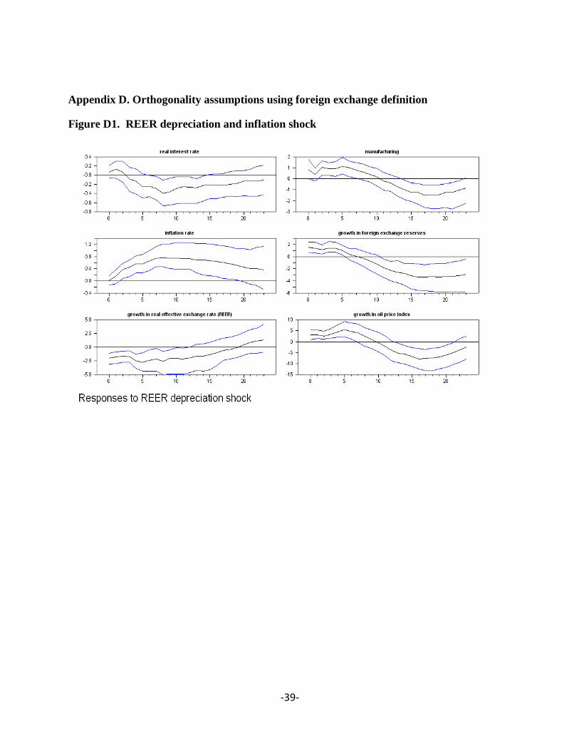
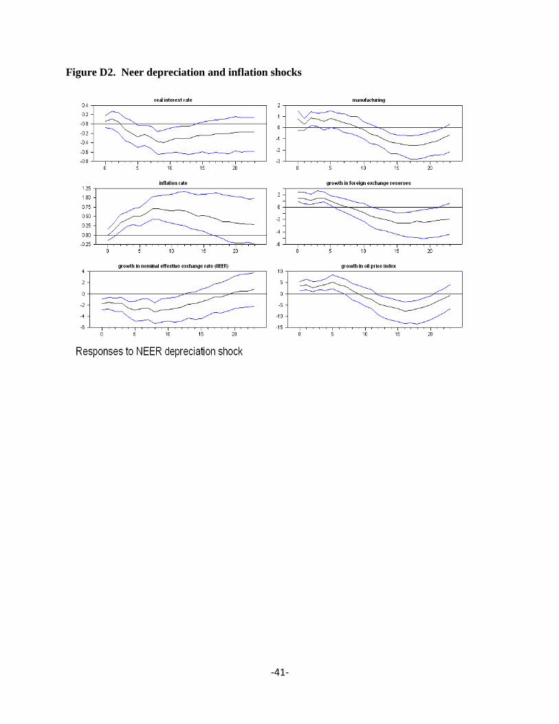
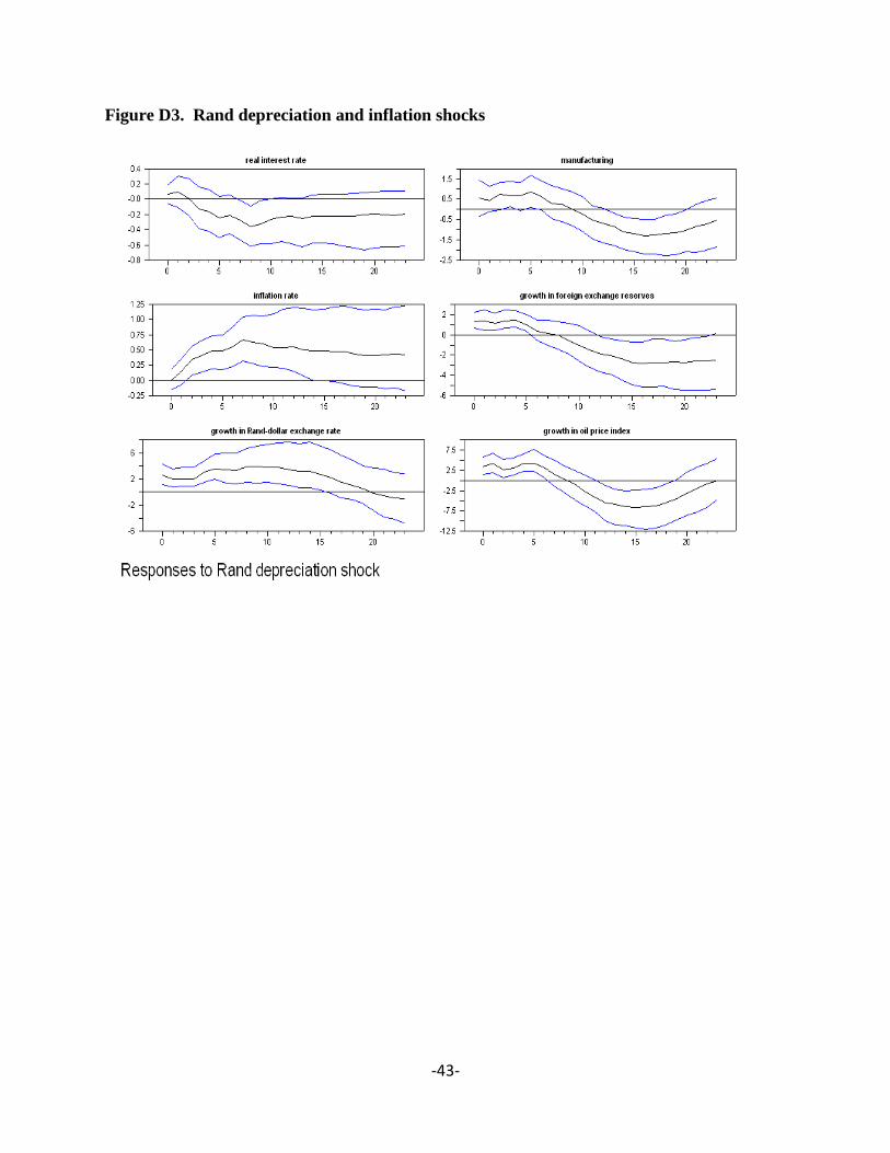
Appendix D. Orthogonality assumptions using foreign exchange definition

Figure D1. REER depreciation and inflation shock

-40-

-41-

Figure D2. Neer depreciation and inflation shocks

-42-

-43-

Figure D3. Rand depreciation and inflation shocks

-44-

-45-

Recent Publications in the Series

nº Year Author(s) Title

133 2011 Mthuli Ncube and Eliphas Ndou Monetary Policy Transmission, House Prices and Consumer

Spending in South Africa: An SVAR Approach

132 2011

Ousman Gajigo, Emelly Mutambatsere and

Elvis Adjei

Manganese Industry Analysis: Implications For Project

Finance

131 2011 Basil Jones

Linking Research to Policy: The African Development

Bank as Knowledge Broker

130 2011 Wolassa L.Kumo Growth and Macroeconomic Convergence in Southern Africa

129 2011 Jean- Claude Berthelemy China’s Engagement and Aid Effectiveness in Africa

128 2011 Ron Sandrey

Hannah Edinger China’s Manufacturing and Industrialization in Africa

127 2011 Richard Schiere

Alex Rugamba Chinese Infrastructure Investments and African integration

126 2011 Mary-Francoise Renard China’s Trade and FDI in Africa

125 2011 Richard Schiere

China and Africa: An Emerging Partnership for

Development? – An Overview of Issues

124 2011 Jing Gu

Richard Schiere Post-crisis Prospects for China-Africa Relations

123 2011

Marco Stampini

Audrey Verdier-Chouchane

Labor Market Dynamics in Tunisia:

The Issue of Youth Unemployment

-46-