Electronic copy available at: https://ssrn.com/abstract=3147101

1126 E. 59th St, Chicago, IL 60637 Main: 773.702.5599

bfi.uchicago.edu

WORKING PAPER · NO. 2018-44

Microeconomic Heterogeneity and Macroeconomic ShocksGreg Kaplan and Giovanni L. ViolanteJune 2018

Microeconomic Heterogeneity and

Macroeconomic Shocks∗

Greg Kaplan‡ Giovanni L. Violante§

June 12, 2018

Abstract

We analyze the role of household heterogeneity for the response of the macroe-conomy to aggregate shocks. After summarizing how macroeconomists haveincorporated household heterogeneity and market incompleteness in the study ofeconomic fluctuations so far, we outline an emerging framework that combinesHeterogeneous Agents (HA) with nominal rigidities, as in New Keynesian (NK)models, that is much better aligned with the micro evidence on consumptionbehavior than its Representative Agent (RA) counterpart. By simulating con-sistently calibrated versions of HANK and RANK models, we convey two broadmessages. First, the degree of equivalence between models crucially depends onthe shock being analyzed. Second, certain interesting macroeconomic questionsconcerning economic fluctuations can only be addressed within HA models, andthus the addition of heterogeneity broadens the range of problems that can bestudied by economists. We conclude by recognizing that the development ofHANK models is still in its infancy and by indicating promising directions forfuture work.

Keywords: Aggregate Shocks, Household Heterogeneity, Incomplete Markets, Model

Equivalence, Representative Agent, Transmission Mechanism.

∗A shorter, non-technical version of this paper with the same title is published in the Journal ofEconomic Perspectives, as part of a special issue of the on ‘The State of Macroeconomics a DecadeAfter The Crisis.’ We are grateful to Felipe Alves for outstanding research assistance and to MarkGertler, David Lopez-Salido, Virgiliu Midrigan, Ben Moll, Matt Rognlie, Tom Sargent and ChristianWolf for comments.‡University of Chicago, IFS and NBER§Princeton University, CEPR, IFS, IZA, and NBER

1 Introduction

In this essay, we discuss the emerging literature that combines heterogeneous agent

models, nominal rigidities and aggregate shocks. This literature opens the door to the

analysis of distributional issues, economic fluctuations, and stabilization policies —all

within the same framework.

Quantitative macroeconomic models have integrated heterogeneous agents and in-

complete markets for nearly three decades. However, they have been mainly used for

the investigation of consumption and saving behavior, inequality, redistributive poli-

cies, economic mobility and other cross-sectional phenomena. Representative agent

models have remained the benchmark in the study of aggregate fluctuations.1

The Great Recession bluntly exposed the shortcomings of the representative-agent

approach to business cycle analysis. A broadly shared interpretation of the Great Re-

cession places its origins in housing and credit markets. The collapse in house prices

affected households differently, depending on the composition of their balance sheets.

The extent to which this wealth destruction translated into a fall in expenditures was

determined by marginal propensities to consume, which are also very heterogeneous

and closely related to households’ access to liquidity (Mian et al., 2013; Kaplan et al.,

2014). Finally, this drop in aggregate consumer demand and the contemporaneous

breakdown in bank lending to businesses (Gertler and Gilchrist, 2017) resulted in a

severe contraction of labor demand which materialized unevenly across different occu-

pations and skill levels. All this took place against the backdrop of a secular rise in

income and wealth inequality.

Thus, portfolio composition, credit, liquidity, marginal propensities to consume,

unemployment risk and inequality were all central to the unfolding of the Great Reces-

sion. Yet these are all issues that one cannot discuss in a representative agent model

(at least not without trivializing them).2

In response to these limitations of the representative agent approach to economic

fluctuations, a new framework has emerged that combines key features of heterogeneous

agents (HA) and New Keynesian (NK) economies. These HANK models offer a much

more accurate representation of household consumption behavior and can generate

1 As we explain later, we attribute this dichotomy both to computational complexity and to somewidely held views on the irrelevance of distributions for aggregate outcomes.

2The need for macroeconomists to move beyond the representative agent fiction in business cy-cle analysis was also emphasized by a number of high officials and governors of central banks inspeeches delivered after the crisis: for example, see the comments from Janet Yellen (2016) of the USFederal Reserve (https://www.federalreserve.gov/newsevents/speech/yellen20161014a.htm),Vitor Costancio (2017) of the European Central Bank (https://www.ecb.europa.eu/press/key/date/2017/html/ecb.sp170822.en.html) and Haruiko Kuroda of the Bank of Japan (https://www.boj.or.jp/en/announcements/press/koen_2017/ko170524a.htm).

2

realistic distributions of income, wealth and, albeit to a lesser degree, household balance

sheets. At the same time, they can accommodate many sources of macroeconomic

fluctuations, including those driven by aggregate demand. In sum, they provide a

rich theoretical framework for quantitative analysis of the interaction between cross-

sectional distributions and aggregate dynamics.

In this article, we outline a state-of-the-art version of HANK based on Kaplan et

al. (2018), together with its representative agent counterpart. We use this HANK

model, calibrated to the US economy, to convey two broad messages about the role of

household heterogeneity for the response of the macroeconomy to aggregate shocks.

The first message is that the similarity between the Representative Agent New

Keynesian (RANK) and HANK frameworks depends crucially on the shock being an-

alyzed. We illustrate this point through a series of examples. In response to a demand

shock arising from a change in household discount factors, HANK and RANK generate

the same aggregate dynamics through largely the same economic mechanisms. In re-

sponse to a technology shock, the two models also generate similar aggregate dynamics,

but through different economic mechanisms. And following fiscal and monetary policy

shocks, the two models generate different aggregate responses. These discrepancies can

be traced to the fact that household consumption is more sensitive to income and less

sensitive to interest rates in heterogeneous agent models than in representative agent

models.

We then turn to our second message: certain important macroeconomic questions

concerning economic fluctuations can only be addressed within heterogeneous agent

models. To make this point, we first look at how in HANK models aggregate de-

mand shocks can have a proper microfoundation, e.g. through unexpected changes in

borrowing capacity or uninsurable income risk. Second, we show how one can learn

about the source and transmission mechanism of aggregate shocks by examining how

they impact households at different parts of the wealth distribution. Third, we illus-

trate how HANK models can be used to understand the effect of aggregate shocks and

stabilization policies on household inequality.

We conclude by suggesting several broad directions for the future development of

HANK models. Throughout this article, we focus on household heterogeneity, so when

we use the term ‘agents’ we refer to ‘households’. There is a parallel literature on firm

heterogeneity and aggregate dynamics which deserves its own separate treatment.3

Here, it suffices to say that many of the points we make on the role of heterogeneity

3For example, see Caballero (1999) and Khan and Thomas (2008) for the debate on how firm-level non-convex adjustment costs influence aggregate investment and Gertler and Gilchrist (1994)and Ottonello and Winberry (2018) for the debate on how firm-level financial constraints affect thetransmission of monetary policy.

3

apply to that literature as well.

2 Heterogeneity and Business Cycles in Macroeconomics, So

Far

Macroeconomics is about general equilibrium analysis. Dealing with distributions,

while at the same time respecting the aggregate consistency dictated by equilibrium

conditions, can be extremely challenging. This explains why in the 1970s, when the

path-breaking work of James Heckman and Daniel McFadden was paving the way

for a rich treatment of cross-sectional heterogeneity in microeconometrics, the focus

in macroeconomics was on developing models where aggregate outcomes would not

depend on distributions. At that time, James Tobin famously defined macroeconomics

as a subject that attains workable approximations by ignoring effects on aggregates

of distributions of wealth and income (Sargent, 2015). Heterogeneity was neutralized

by assuming either identical initial conditions right off-the-bat, or special preference

specifications (through Gorman aggregation), or complete markets (through Negishi

aggregation).

Heterogeneous agent incomplete-markets models with non-trivial distributions of

households appeared in the mid 1980s. Ljungqvist and Sargent (2004) baptized this

class of models “Bewley models” because Truman Bewley was the first to explore

the equilibrium properties of these economies (Bewley, 1983). Throughout the 1990s,

the seminal work of Imrohorolu (1989), Huggett (1993), Aiyagari (1994), and Rıos-

Rull (1995), among others, laid the foundations for a new workhorse of quantitative

macroeconomics that expanded the Bewley model and recasted it in the recursive

language developed by Robert Lucas, Edward Prescott, Thomas Sargent, and Nancy

Stokey, among others. To quote from Aiyagari (1994, p.1), its distinctive feature was

that “aggregate behavior is the result of market interaction among a large number of

agents subject to idiosyncratic shocks. [...] This contrasts with representative agent

models where individual dynamics [...] coincide with aggregate dynamics [...].”

This framework combines two building blocks. On the production side, a repre-

sentative firm with a neoclassical production function rents capital and labor from

households to produce a final good. On the household side, a continuum of agents

each solve their own income fluctuation problem – the problem of how to smooth con-

sumption when income is subject to random shocks and the only available financial

instrument is saving (and possibly limited borrowing) in a risk-free asset (e.g., Schecht-

man, 1976). The equilibrium real interest rate is determined by equating households’

supply of savings to firms’ demand for capital.

4

The main motivation for modeling consumer behavior along these lines was the

rapidly mounting empirical evidence, based on longitudinal household survey data,

that most households fail in their efforts to perfectly smooth consumption (Hall, 1978;

Cochrane, 1991; Attanasio and Davis, 1996), a finding that time has only reinforced.

Heterogeneous agent models allowed investigation of imperfect consumption insurance

– its extent, reasons, and effects for the macroeconomy.

Reading through the recent surveys of this literature (e.g, Heathcote et al., 2009;

Guvenen, 2011; Quadrini and Rıos-Rull, 2015; Benhabib and Bisin, 2016; De Nardi

and Fella, 2017), one is struck by the fact that while heterogeneous agent models have

been routinely used to study questions pertaining to income and wealth inequality,

redistribution, economic mobility and tax reforms, until recently they had not been

much used to study business cycles. The reason, we think, is twofold: computational

complexity and a result known as “approximate aggregation”.

Computational complexity arises because in the recursive formulation of heteroge-

neous agent models with aggregate shocks, households require a lot of information in

order to solve their dynamic optimization problems: each household must not only

know its own place in the cross-sectional distribution of income and wealth, but must

also understand the equilibrium law of motion for the entire wealth distribution. Un-

der rational expectations, this law of motion is an endogenous equilibrium object and

solving for it is a computationally intensive process.

The first to successfully tackle this challenge were Krusell and Smith (1998), who

pioneered the most well-known method and applied it to a simple heterogeneous agent

economy with aggregate technology shocks. Despite recent advances in computing

power and numerical methods, applying their method to the most interesting versions

of heterogeneous agent economies remains challenging. In recent years, several new

computational methods have been proposed that have widened the set of models that

can be accurately solved. These include mixtures of projection and perturbation (Re-

iter, 2009), mixtures of finite difference methods and perturbation (Ahn et al., 2017),

adaptive sparse grids (Brumm and Scheidegger, 2017), polynomial chaos expansions

(Prohl, 2017), machine learning (Duarte, 2018; Fernandez-Villaverde et al., 2018) and

linearization with impulse-response functions (Boppart et al., 2017). Which of these,

or other, methods will ultimately prevail is an open question.

The “approximate aggregation” result, uncovered by Krusell and Smith (1998),

states that in many heterogeneous agent models, the mean of the equilibrium wealth

distribution is sufficient to forecast all relevant future prices. The underlying logic is

compelling: what matters for the aggregate dynamics of interest rates are the actions

of households who hold the bulk of the wealth in the economy. Those rich households

5

are well-insured against fluctuations and have saving functions that are approximately

linear in wealth. Households that are close to the borrowing constraint, where the

saving functions have curvature, are largely irrelevant in terms of their contribution to

the aggregate capital stock and consumption. Krusell and Smith (1998) showed that

in a benchmark version of the heterogeneous agent model, the aggregate dynamics of

output, consumption and investment in response to a shock to total factor productivity

are almost identical to their counterpart representative agent model.

Approximate aggregation has proved surprisingly robust over time and has led many

economists to conclude that aggregate dynamics in representative and heterogeneous

agent models are essentially equivalent. As we show in this article, this interpretation

of the original Krusell-Smith insight is inaccurate. Because of this misunderstand-

ing, deviating from the representative agent approach was perceived by much of the

profession as incurring a high computational cost for only little benefit. As a conse-

quence, quantitative heterogeneous agent models rarely crossed paths with the study

of business cycles.

The Great Recession put consumption, income, and wealth distributions back at the

center stage of business cycles analysis and undermined this perception. Economists

began to realize that two critical ingredients were needed for a coherent analysis of

fluctuations and stabilization policy: (i) household heterogeneity and (ii) a framework

that can accommodate aggregate demand shortfalls. In response, a number of macro

researchers chose to address this gap in the most natural way: by combining key

features of heterogeneous agent models and New Keynesian models.

3 Heterogeneous Agent New Keynesian (HANK) Models

In this section, we first argue that modeling household heterogeneity is important,

by itself and in conjunction with nominal rigidities. Next, we discuss some early

applications of HANK models. Finally, we outline this new framework in detail, setting

the stage for the second part of our article where we contrast HANK and RANK models.

3.1 Heterogeneity is Key for Matching Facts about Consump-tion Behavior

Consumption behavior in representative agent models is inconsistent with empirical

evidence. A representative household is essentially a permanent income consumer

facing an intertemporal budget constraint. As such, its consumption is extremely

responsive to changes in current and future interest rates, but barely responds to

transitory changes in income.

6

The high sensitivity of consumption to interest rates is not well-supported by macro

or micro data. Analyses using aggregate time-series data typically find that, after

controlling for aggregate income, consumption is not very responsive to changes in

interest rates (Deaton, 1987; Campbell and Mankiw, 1989; Yogo, 2004; Canzoneri et

al., 2007). A number of studies reveal that both the sign and size of the effect of

changes in interest rates on consumption depend on households’ net asset positions

(Floden et al., 2016; Cloyne et al., 2017). Empirical analyses using micro data on

household portfolios also conclude that a sizable fraction of households (around one-

third in the United States) hold close to zero liquid wealth or are near their borrowing

limits (Kaplan et al., 2014). Empirically, these households do not react to movements

in interest rates (Vissing-Jørgensen, 2002).

The implication from a representative agent model that consumption is insensi-

tive to transitory income shocks is also inconsistent with the vast micro empirical

literature surveyed by Jappelli and Pistaferri (2010). This literature has employed

three approaches to identify exogenous income shocks. The first approach seeks quasi-

experimental settings where natural variation generates randomness in either the re-

ceipt, amount, or timing of gains or losses. Examples include firm-level shocks, unem-

ployment due to plant closings, stimulus payments and lottery winnings (e.g., Browning

and Crossley, 2001; Johnson et al., 2006; Broda and Parker, 2014; Misra and Surico,

2014; Fagereng et al., 2016; Baker, 2018). The second approach extracts the consump-

tion response to the transitory component of regular income fluctuations by assuming a

particular statistical process for income and exploiting assumptions about how income

and consumption should co-vary (e.g., Blundell et al., 2008; Heathcote et al., 2014; Ka-

plan et al., 2014). The third approach uses survey questions that ask respondents about

how their expenditures would change in response to actual or hypothetical changes in

their budgets (e.g., Shapiro and Slemrod, 2003; Christelis et al., 2017; Fuster et al.,

2018).

This collective body of evidence on marginal propensities to consume (MPCs) points

towards: (i) sizable average MPCs out of small, unanticipated, transitory income

changes; (ii) larger MPCs for negative than for positive income shocks; (iii) small

MPCs in response to announcements about future income gains; and (iv) substantial

heterogeneity in MPCs that is correlated with access to liquidity. None of these four

features are in line with the consumption behavior in representative agent models.

Heterogeneous agent models with incomplete markets can, instead, reproduce many

of these aspects of consumption behavior. Households who are at a kink in their budget

sets (generated, for example, by a borrowing limit or by a wedge between interest

rates on liquid savings and unsecured borrowing) have high MPCs out of transitory

7

income shocks and do not respond to small changes in interest rates. For households

who are close to a kink, exposure to uninsurable income risk raises the possibility of

hitting the kink in the future which shortens their effective time horizon, dampens

the intertemporal substitution channel and raises their MPC (Carroll, 1997). For all

other households, a fall in real rates leads to an increase in expenditures through

intertemporal substitution, but there is also a counteracting income effect that can be

especially strong for wealthy households.

3.2 Heterogeneity Restores Keynesian Insights into the NewKeynesian Model

During the last couple of decades, the New Keynesian model has become the refer-

ence paradigm for economists working for central banks and governments who need

a micro-founded framework to think about the aggregate and welfare effects of fiscal

and monetary policy interventions (Clarida et al., 1999; Woodford, 2003). In a New

Keynesian model, monopolistically competitive firms produce differentiated goods and

face costs of adjusting prices. Because prices are sticky in the short-run, money supply

can affect aggregate demand and monetary policy can have real effects. Over time, this

research program has given rise to large scale models which can accommodate multiple

real and nominal aggregate shocks.

However, since the baseline New Keynesian model employs a representative agent,

its implied consumption dynamics feature strong intertemporal substitution and weak

income sensitivity. Thus, somewhat paradoxically and in spite of its name, the mech-

anism by which aggregate demand affects aggregate output in the standard New Key-

nesian model differs markedly from the ideas typically associated with John Maynard

Keynes (namely, the equilibrium spending multiplier). For these reasons, Cochrane

(2015) has suggested that it would be more appropriate to call this model the sticky-

price intertemporal-substitution model.

The higher average MPC, more realistic distribution of MPCs, and lower sensitivity

to interest rates make the general equilibrium effects of aggregate demand fluctuations

much more salient in the heterogeneous agent version of the New Keynesian model

than in the representative agent version.

3.3 HANK: Early Examples

The first examples of heterogeneous agent New Keynesian models appeared in the

immediate wake of the Great Recession. These models were designed to address the

origins of the crisis, its propagation, and the observed policy responses, all aspects in

8

which household heterogeneity in terms of income, wealth, and balance sheets plays a

central role. Oh and Reis (2012) study the extent to which fiscal stimulus in the form

of targeted transfers to households alleviated the costs of the recession. Guerrieri and

Lorenzoni (2017) examine the impact of a tightening of household borrowing constraints

on aggregate demand and output. McKay and Reis (2016) investigate the role of

automatic stabilizers in dampening macroeconomic fluctuations when monetary policy

is active and when it is constrained by the zero-lower-bound. Similarly, Krueger et

al. (2016) examine the effectiveness of unemployment insurance in mitigating the fall

in aggregate expenditures during the crisis. McKay et al. (2016), Werning (2015),

and Kaplan et al. (2018) study the effectiveness of various forms of monetary policy

including forward guidance, an instrument used by central banks to stimulate aggregate

demand when the zero lower bound is binding. Den Haan et al. (2017) and Bayer et

al. (2017) argue that the precautionary saving response to an increase in labor market

risk causes households to substitute away from consumption expenditures into non-

productive, safe assets (such as government bonds), which can trigger a demand-driven

recession.

These models differ in many important details, but they are all HANK models:

they combine New Keynesian-style nominal rigidities with household heterogeneity

and market incompleteness.

3.4 HANK: Central Elements

In the remainder of the paper we focus on a version of HANK developed by Kaplan,

Moll and Violante (2018) and demonstrate how the shocks studied in these papers can

all be understood in a single, consistent framework. The household block of the model

is based on Kaplan and Violante (2014). Households face uninsurable labor productiv-

ity risk and make labor supply, consumption, and savings decisions. Unlike the models

in the aforementioned papers, households have access to two assets: (i) a low-return

liquid asset that represents holdings of cash, checking accounts and government bonds;

and (ii) a high-return illiquid asset that is subject to a transaction cost and represents

equities (which are mostly held in not-so-liquid retirement accounts), privately-owned

businesses and net housing assets. Unsecured credit is allowed through negative po-

sitions in the liquid asset. We discuss the advantages of the two-asset HANK model

over one-asset HANK models after describing the environment. The wage and both

rates of return are determined in equilibrium by relevant market clearing conditions.

The remaining blocks of the model follow closely the New Keynesian tradition. The

model is developed and solved in continuous time, using the finite-difference methods

9

proposed by Achdou et al. (2017).4

Households The economy is populated by a continuum of households of measure

one, who die at an exogenous rate ζ. Households receive a utility flow from consum-

ing ct and disutility flow from supplying labor ht. We assume a unitary elasticity of

intertemporal substitution and a constant Frisch labor supply elasticity ε. Preferences

are time-separable and, conditional on surviving, the future is discounted at rate ρ,

E0

∫ ∞0

e−(ζ+ρ)t

[log ct − ψ

h1+1/εt

1 + 1/ε

]dt, (1)

where the expectation is taken over realizations of idiosyncratic productivity shocks zt.

Households can allocate their wealth between liquid assets bt and illiquid assets

at, both of which are real. Assets of type at are illiquid in the sense that households

must pay a transaction cost when depositing into or withdrawing from their illiquid

account. We use dt to denote a household’s deposit rate (with dt < 0 corresponding

to withdrawals) and χ(dt, at) to denote the flow cost of depositing at a rate dt for a

household with illiquid holdings at. The function χ(d, a) is increasing and convex in

|d| and is decreasing and concave in a. Households can borrow in liquid assets up to

an exogenous limit b at an interest rate that is higher than the interest rate on liquid

saving. We interpret this spread as an exogenous cost of financial intermediation and

define the interest rate schedule faced by households as rbt (bt). Short positions in illiquid

assets are not allowed.

Households’ budget constraints are thus given by

·bt = (1− τt)wtztht + rbt (bt)bt + Tt − dt − χ(dt, at)− ct (2)·at = rat at + dt (3)

bt ≥ −b, at ≥ 0. (4)

Liquid assets increase due to labor earnings (net of a proportional labor income tax

τt), interest payments on liquid assets and lump-sum government transfers Tt, and de-

crease due to net deposits into the illiquid account, transaction costs and consumption

expenditures. Illiquid assets increase due to interest payments plus net deposits.

4Our presentation of the model is purposefully kept simple and omits some details. For a morecomprehensive description of this framework and its parameterization, see Kaplan, Moll and Violante(2018).

10

Firms A representative final-good producer combines a continuum of intermediate

inputs through a constant elasticity aggregator. Each intermediate good is produced

by a monopolistically competitive firm using capital and labor rented from households

in competitive input markets. Intermediate producers choose their price to maximize

profits subject to quadratic price adjustment costs as in Rotemberg (1982). The solu-

tion to the dynamic pricing problem yields a standard forward-looking New Keynesian

Phillips curve that links current inflation to the future dynamics of marginal costs.

The illiquid asset comprises both productive capital and shares that are claims on the

equity of an aggregate portfolio of intermediate firms (whose price qt reflects the value

of the discounted future stream of monopoly profits net of price adjustment costs).5

Government and monetary authority The government raises revenue through a

proportional tax on labor income and uses it to finance purchases of final goods Gt, pay

lump-sum transfers Tt and pay interest on its outstanding real debt Bt, subject to an

intertemporal budget constraint. The government is the only provider of liquid assets

in the economy. The monetary authority sets the nominal interest rate it on liquid

assets according to the simple Taylor rule it = rb + φπt. Given inflation πt and the

nominal interest rate, the real return on the liquid asset is determined by the Fisher

equation rbt = it − πt.

Equilibrium in asset markets The equilibrium returns rbt and rat clear the bond

market and the illiquid asset market respectively. In steady state, rat > rbt because

households command an illiquidity premium in order to accumulate illiquid assets,

since they foresee having to pay a transaction cost on future withdrawals. In addition,

the presence of uninsurable idiosyncratic risk and incomplete markets generates a pre-

cautionary motive that gives rise to an endogenous preference for risk-free liquid assets

over risky or illiquid assets. We return to this point in Section 4.6.

Heterogeneity Requires Making Additional Assumptions In concluding the

description of the model, it is worth emphasizing that several modeling choices that

are inconsequential in RANK models can matter tremendously for the behavior of

HANK models. In HANK, because of borrowing constraints and MPC heterogeneity,

both the timing and distribution of the fiscal transfers that are needed to balance

the government budget constraint in the wake of a shock matter. In RANK, because

5We assume that, within the illiquid account, resources can be freely moved between capital andequity, an assumption which allows us to reduce the dimensionality of the asset space. We also assumethat a fixed fraction of dividends is reinvested in the illiquid account, with the remainder paid intohouseholds’ liquid account, as in Kaplan, Moll and Violante (2018).

11

of Ricardian Equivalence, the choice of fiscal rule does not matter. Similarly, the

distribution of claims to firm profits, both across households and between liquid and

illiquid assets, matters in HANK, whereas in RANK profits are simply rebated to the

representative household.6 This also implies that in RANK models there is a unique

stochastic discount factor for firms to use when setting prices, but in HANK models

there is no unique discount factor. Moreover, in HANK, an assumption is needed about

the extent to which fluctuations in labor demand are concentrated among different

households, whereas in RANK no such assumption is necessary. Finally, because of

the precautionary saving motive and occasionally binding borrowing constraint, in

HANK the cyclicality of idiosyncratic uncertainty and access to liquidity are important

determinants of the effects of aggregate shocks to household consumption (Acharya and

Dogra, 2018; Werning, 2015).

On the one hand, the sensitivity of HANK to these assumptions complicates the

analysis and highlights important areas where micro data must be confronted. On the

other hand, the assumptions about all these issues implicit in RANK models have little

empirical support.7

3.5 Role of the Two Assets for Consumption Behavior

Virtually all of the existing HANK literature uses models with a single asset. However,

we adopt a the two-asset model because it is more successful at capturing key features

of microeconomic consumption behavior.

The co-existence of a low-return liquid asset and a high-return illiquid asset creates

the conditions for the emergence of wealthy hand-to-mouth households (who hold little

or no liquid wealth despite owning sizable amounts of illiquid assets) alongside poor

hand-to-mouth households (who hold little net worth). The model is able to replicate

the observation that around one-third of US households are hand-to-mouth with high

MPCs and, among these, around two-thirds are wealthy hand-to-mouth and one-third

are poor hand-to-mouth (Kaplan et al., 2014). The remaining households hold sufficient

liquid wealth that their consumption dynamics are similar to those of the representative

agent.

This existence of both types of hand-to-mouth households improves the fit of the

model with respect to the responsiveness of consumption to interest rates and transi-

tory income shocks. The two-asset model generates an average quarterly MPC out of

6Broer et al. (2016) offer an enlightening discussion of how the New Keynesian transmission mech-anism is influenced by the assumptions that determine how profits get distributed across households.

7See Kaplan et al. (2018) for details on the specific assumptions made in our baseline HANK modelwith respect to all these dimensions.

12

0400

0.05

0.1

300 20

0.15

0.2

10200

0.25

0.3

0100-10

0

Figure 1: Distribution of MPC out of a windfall income of $500 in the calibrated model

small income windfalls of around 15 to 20 percent, as well as substantial heterogeneity

in MPCs driven by heterogeneity in liquid wealth holdings across households. These

features are illustrated in Figure 1, which shows quarterly MPCs out of $500 for house-

holds with different amounts of liquid and illiquid wealth. The high MPCs for wealthy

hand-to-mouth households is clearly visible as the ridge at zero liquid wealth. This

level and distribution of MPCs is in line with the large body of evidence discussed

earlier, as well as with more recent evidence in the context of the Great Recession

(Mian et al., 2013).

For comparison, the average MPC in an otherwise similar representative agent

model is approximately equal to the discount rate, which is around 0.5 percent quar-

terly. When parameterized to match the same ratio of net worth to average income as

in the data (and as in the two-asset model), the average quarterly MPC in the one-asset

model is around 4 percent, which is eight times higher than in the representative agent

model, but still much lower than empirical estimates.

Researchers have proposed modifications to the one-asset model to increase the av-

erage MPC to empirically realistic levels. One approach is to ignore all illiquid wealth

and choose the household discount factor to generate the same ratio of liquid wealth to

average income as in the data. Besides grossly misrepresenting observed household bal-

ance sheets, this approach also precludes the model from including capital – which is a

13

crucial ingredient when analyzing macroeconomic dynamics in general equilibrium. A

second approach (Carroll et al., 2017; Krueger et al., 2016) is to introduce enough het-

erogeneity in discount factors so that there are some very patient households that drive

capital accumulation, together with some very impatient households that have a high

MPC (although, even with heterogeneity in discount factors, a low-wealth calibration

is usually required in order to generate a high aggregate MPC).

A problem with both these approaches is that, in order to generate realistic MPCs,

the one-asset models feature many more poor hand-to-mouth households than are in

the data. By abstracting from the illiquid assets held by the wealthy hand-to-mouth,

these models also miss potentially important exposure of household consumption to

fluctuations in returns to illiquid assets.

3.6 RANK: The Representative Agent Counterpart

Many of the results in the next section are framed in terms of a comparison between

HANK and a corresponding RANK model. To allow for a clean comparison between the

two models, we adopt a RANK model with the same two-asset structure and the same

functional forms for preferences, technology, transaction costs and price adjustment

costs, and the same production side, government and monetary authority, as in HANK.

The only difference is the absence of any form of household heterogeneity.8 Importantly,

despite the two-asset structure, our version of RANK retains Ricardian neutrality.

4 Comparison Between RANK and HANK

In this section, we compare the responses of RANK and HANK to a series of aggregate

shocks that are common in the study of business cycles. We assume that each economy

is initially in its steady state and is then hit by a one-time, unanticipated shock (an

‘MIT shock’) that is persistent and mean-reverting. After the shock, the economies

eventually return to their original steady-states. Since the key difference between the

8We calibrate the RANK parameters in order to match the same aggregate targets as in HANK.Our strategy for choosing the two transaction cost parameters (scale, curvature) in RANK is neces-sarily different though, because in HANK we choose them to replicate moments of the cross-sectionaldistribution of liquid and illiquid assets, for which the RA model does not make predictions. Wechoose the scale parameter of the adjustment cost function so that total transaction costs as a frac-tion of output in steady-state are the same as in HANK. The curvature parameter determines theresponsiveness of aggregate deposits to the gap in rates of return between the two assets. Hence, wechoose the curvature parameter so that the elasticity of aggregate deposits to a change in the realliquid rate rbt is the same as in HANK (keeping all other prices, including rat , fixed at their steady-state values). This ensures that, in partial equilibrium, investment in the two models has the samesensitivity to the liquid interest rate.

14

two models is on the household side, we focus our attention on the response of aggregate

consumption Cm := {Cmt }t≥0, where m ∈ {HA,RA} indexes the models.

In HANK, we need to make an assumption about the timing of the changes in

lump-sum transfers Tt that are needed to maintain balance of the government budget

constraint in the wake of the shocks. We assume that in the short-run, this adjustment

takes place almost entirely through changes in the level of government debt (which

translates into changes in the supply of liquid assets). In the long-run, lump-sum

transfers adjust. We call this form of fiscal adjustment the baseline fiscal rule.

4.1 Notions of Equivalence Between RANK and HANK

The impulse response function (IRF) of aggregate consumption to a given shock can

be constructed by aggregating the optimal decisions of households when faced with the

equilibrium prices and transfers induced by the shock. It is thus useful to make explicit

the dependence of the IRF on a vector of equilibrium objects, Θm := {Θmτ }τ≥0. This

vector includes three types of variables: (i) the shock itself η := {ηt}t≥0 which is the

same in RANK and HANK; (ii) the path of equilibrium prices(w, rb, ra, q

)min each

model m; and (iii) the path for lump-sum transfers Tm in each model.9 Let j = 1, ..., J

index the elements of this vector. Then, from the definition of an IRF, we can express

the change in consumption at date t as

dCmt =

J∑j=1

∫ ∞τ=0

∂Cmt

∂Θjτ

dΘmjτdτ for t = 0, ...,∞. (5)

In order to compare the IRF in RANK and HANK, we find it useful to define

three notions of equivalence between the two models. We say that the two models are

non-equivalent when the IRFs are different. We say that the two models are weakly

equivalent when the IRFs are the same but the transmission mechanisms of the shock

are different. Finally, we say that the two models are strongly equivalent when both

the IRFs and the transmission mechanisms are the same. In other words, RANK and

HANK are strongly equivalent only if they produce the same IRF to the same shock,

for the same reasons.

Comparing IRFs across models, and hence identifying non-equivalence, is simple.

Comparing transmission mechanisms, which is needed in order to distinguish between

weak and strong equivalence, is more involved and is open to some interpretation. We

9In both models, the shock itself enters this function only if it directly enters the household problem.For example, this is the case for a preference shock but not for a TFP shock. In HANK, each componentof ΘHA determines the dynamics of aggregate consumption both through its effect on consumptionpolicy rules and its effect on the distribution of households.

15

propose three criteria for deciding whether the transmission mechanism is the same in

the two models. First, we assess whether the IRF decomposition is the same. This

means decomposing the IRF in (5) into the contributions of each of the J terms in the

summation. This decomposition identifies which features of the household problem in

each model (wages, interest rate, transfers, etc.) drive the change in the consumption

response to the shock.

Second, we asses whether the PE-GE discrepancies are the same. This means

decomposing the difference between the two IRFs into a component that is due to

different movements in equilibrium prices (the GE discrepancy) and a component that

is due to different sensitivity to the same movements in prices (the PE discrepancy).

Formally, we can express the difference in IRFs between the two models as

dCHAt − dCRA

t =J∑j=1

∫ ∞0

∂CHAt

∂Θjτ

(dΘHA

jτ − dΘRAjτ

)dτ︸ ︷︷ ︸

GE discrepancy

+J∑j=1

∫ ∞0

(∂CHA

t

∂Θjτ

− ∂CRAt

∂Θjτ

)dΘRA

jτ dτ︸ ︷︷ ︸PE discrepancy

. (6)

Third, we assess the sensitivity to the fiscal rule. Recall that each IRF is conditional

on a particular choice of fiscal rule that specifies the timing of the adjustment in

transfers needed to balance the intertemporal government budget constraint. Due

to Ricardian equivalence, alternative choices for this rule have no effect on the IRF

in RANK. However, different rules can potentially have large effects on the IRF in

HANK.

In light of these criteria, we define HANK and RANK to be strongly equivalent

with respect to a shock when, in addition to the IRFs being the same, the IRF de-

compositions are similar, both the GE and PE discrepancies are small, and the IRF

in HANK is not sensitive to the choice of fiscal rule. When these criteria hold, we say

that the transmission mechanism of the shock is similar across the two models.

Next, we analyze demand, productivity and monetary shocks. The demand shock

is a shock to the marginal utility of consumption, the productivity shock is a shock to

the level of TFP and the monetary shock is a shock to the innovation in the Taylor

rule. For consistency, we consider contractionary shocks whose size and persistence are

chosen to generate a similar drop in aggregate consumption in RANK over the first

quarter. It turns out that these three canonical shocks in business cycle analysis offer

stark examples of the different degrees of equivalence.

16

5 10 15 20-0.8

-0.6

-0.4

-0.2

0

0.2

5 10 15 20-0.8

-0.6

-0.4

-0.2

0

0.2

5 10 15 20-0.8

-0.6

-0.4

-0.2

0

0.2

5 10 15 20-0.4

-0.2

0

0.2

0.4

0.6

5 10 15 20-0.4

-0.2

0

0.2

0.4

0.6

5 10 15 20-0.8

-0.6

-0.4

-0.2

0

0.2

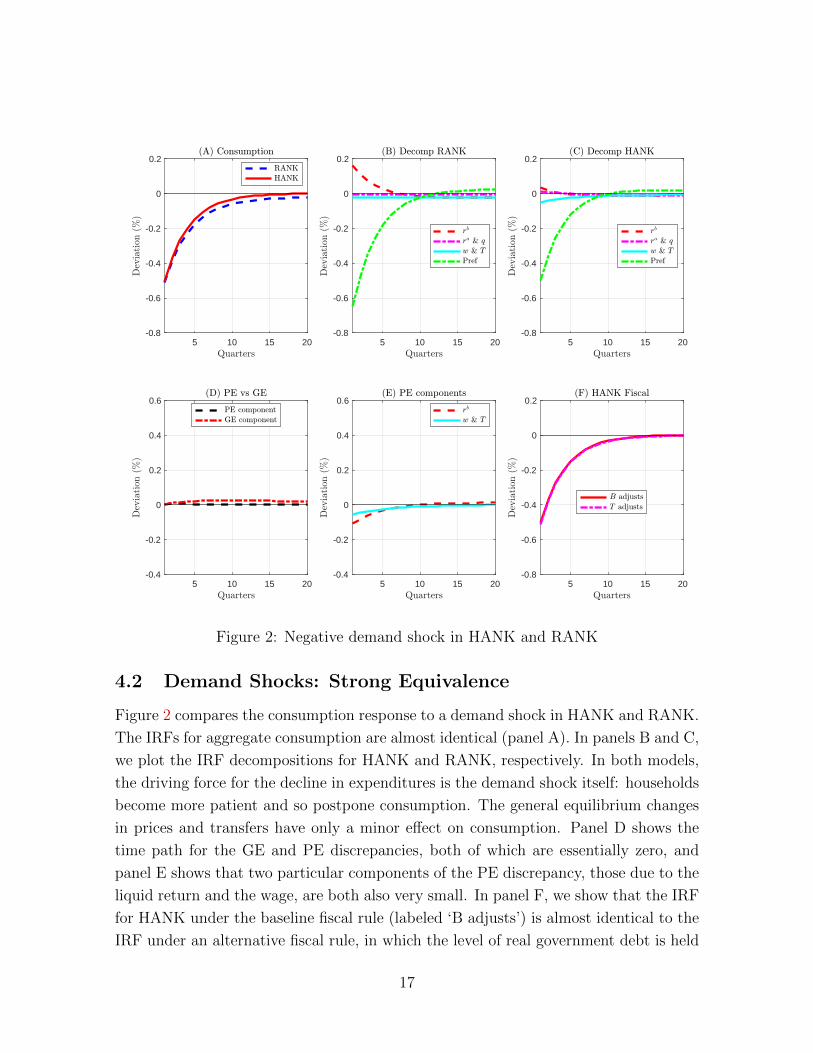
Figure 2: Negative demand shock in HANK and RANK

4.2 Demand Shocks: Strong Equivalence

Figure 2 compares the consumption response to a demand shock in HANK and RANK.

The IRFs for aggregate consumption are almost identical (panel A). In panels B and C,

we plot the IRF decompositions for HANK and RANK, respectively. In both models,

the driving force for the decline in expenditures is the demand shock itself: households

become more patient and so postpone consumption. The general equilibrium changes

in prices and transfers have only a minor effect on consumption. Panel D shows the

time path for the GE and PE discrepancies, both of which are essentially zero, and

panel E shows that two particular components of the PE discrepancy, those due to the

liquid return and the wage, are both also very small. In panel F, we show that the IRF

for HANK under the baseline fiscal rule (labeled ‘B adjusts’) is almost identical to the

IRF under an alternative fiscal rule, in which the level of real government debt is held

17

5 10 15 20

-0.8

-0.6

-0.4

-0.2

0

5 10 15 20

-0.8

-0.6

-0.4

-0.2

0

5 10 15 20

-0.8

-0.6

-0.4

-0.2

0

5 10 15 20-0.4

-0.2

0

0.2

0.4

0.6

5 10 15 20-0.4

-0.2

0

0.2

0.4

0.6

5 10 15 20

-0.8

-0.6

-0.4

-0.2

0

Figure 3: Negative TFP shock in HANK and RANK

fixed at its steady-state value and lump-sum transfers adjust to balance the government

budget constraint in every instant (labeled ‘T adjusts’). Overall, the demand shock

offers a clear-cut example of strong equivalence: both the aggregate response to the

shock and its transmission mechanism are very similar in the two models.

4.3 Total Factor Productivity Shocks: Weak Equivalence

Figure 3 compares the consumption response to a TFP shock in HANK and RANK.

As with the demand shock, the IRFs for the two models lie almost on top of each

other (panel A). However, unlike the demand shock, panels B and C show that the

transmission mechanism for the TFP shock is very different in the two economies. In

RANK (panel B), the fall in consumption is driven entirely by intertemporal substitu-

tion in response to the rise in the liquid interest rate. The drop in productivity raises

18

marginal costs and inflation, to which the central bank reacts by tightening monetary

policy. The representative household responds to the higher interest rate by increasing

liquid savings and postponing consumption. In HANK (panel C), the change in inter-

est rates accounts for less than half of the fall in consumption. Instead, consumption

falls mostly because disposable household income falls and, because of the non-trivial

MPCs in HANK, households respond by cutting consumption.10

Panel D shows that both the GE and PE discrepancies are non-zero, and Panel E

shows that both components of the PE discrepancy are large in absolute value. The

positive PE discrepancy from the liquid rate reflects the fact that consumption falls

less in response to the increase in interest rates in HANK than in RANK. The negative

PE discrepancy from the wage reflects the fact that consumption falls more in response

to the drop in disposable household income in HANK than in RANK. As discussed

in Section 3.5, the high aggregate MPC out of income and low sensitivity to interest

rates are hallmarks of the two-asset HA model. Overall, the TFP shock is an example

of weak equivalence.

4.4 Monetary Shock: Non-Equivalence

Figure 4 compares the consumption response to a monetary shock in HANK and

RANK. In the first quarter after the shock, consumption drops by almost 50% more

in RANK than in HANK (panel A). Moreover, as explained in detail by Kaplan et al.

(2018), the transmission mechanism for monetary policy is very different in the two

models. In RANK, the direct intertemporal substitution channel due to the rise in

the real liquid rate accounts for virtually the whole effect (panel B). In HANK, the

drop in consumption due to the fall in disposable income plays a role that is at least

as important as the substitution channel. Panels D and E illustrate that the PE dis-

crepancy, which reflects different sensitivities of household consumption to wages and

interest rates, drives the gap between the two IRFs. The GE discrepancy is, instead,

much smaller, reflecting the fact that equilibrium prices move similarly in the two mod-

els. Finally, panel F shows that the dynamics of aggregate consumption depend on

the assumed fiscal rule in HANK. When the government immediately cuts transfers in

order to finance the required higher interest payments on its debt (‘T adjusts’ case),

consumption drops more sharply for two reasons. First, lump-sum transfers are an

especially large component of income for poor, high MPC households (a manifesta-

tion of the redistribution channel highlighted by Auclert (2017)). Second, the drop

10As explained in Gali (1999), in RANK models, wages and hours rise in response to a contractionaryTFP shock. This feature of NK models remains present in HANK. The fall in disposable householdincome is due to the fall in firm profits.

19

5 10 15 20

-0.8

-0.6

-0.4

-0.2

0

5 10 15 20

-0.8

-0.6

-0.4

-0.2

0

5 10 15 20

-0.8

-0.6

-0.4

-0.2

0

5 10 15 20-0.4

-0.2

0

0.2

0.4

0.6

5 10 15 20-0.4

-0.2

0

0.2

0.4

0.6

5 10 15 20

-0.8

-0.6

-0.4

-0.2

0

Figure 4: Negative monetary shock (innovation to the Taylor rule) in HANK andRANK

in consumption further amplifies the fall in wages and disposable income through an

aggregate demand multiplier.

We conclude this section by comparing our analysis to Werning (2015). His main

‘as if’ result is one of weak equivalence between the RA and HA model for the response

of aggregate consumption to a monetary shock. His benchmark HA model is purpose-

fully crafted so that the IRF for consumption following a change in the real rate is

exactly the same in the two models. The weaker partial equilibrium intertemporal

substitution response to the change in interest rates in the HA model is exactly offset

by a stronger aggregate demand response in general equilibrium. Werning explains

how departures from his benchmark model can lead to a larger or smaller aggregate

consumption response to the monetary shock in HANK relative to RANK. Our ver-

20

sion of HANK features several such departures, which explains why in our calibrated

economy monetary shocks are examples of non-equivalence.

Our point is not that these three shocks necessarily display the aforementioned

respective degrees of equivalence. Rather we want to illustrate that for our calibrated

two-asset HANK model, which represents the state-of-the-art in many dimensions,

these degrees of equivalence obtain. It is likely possible to reverse engineer artificial

economies that can generate weak equivalence for all three shocks, similarly to Wern-

ing’s results for exogenous interest rate movements.

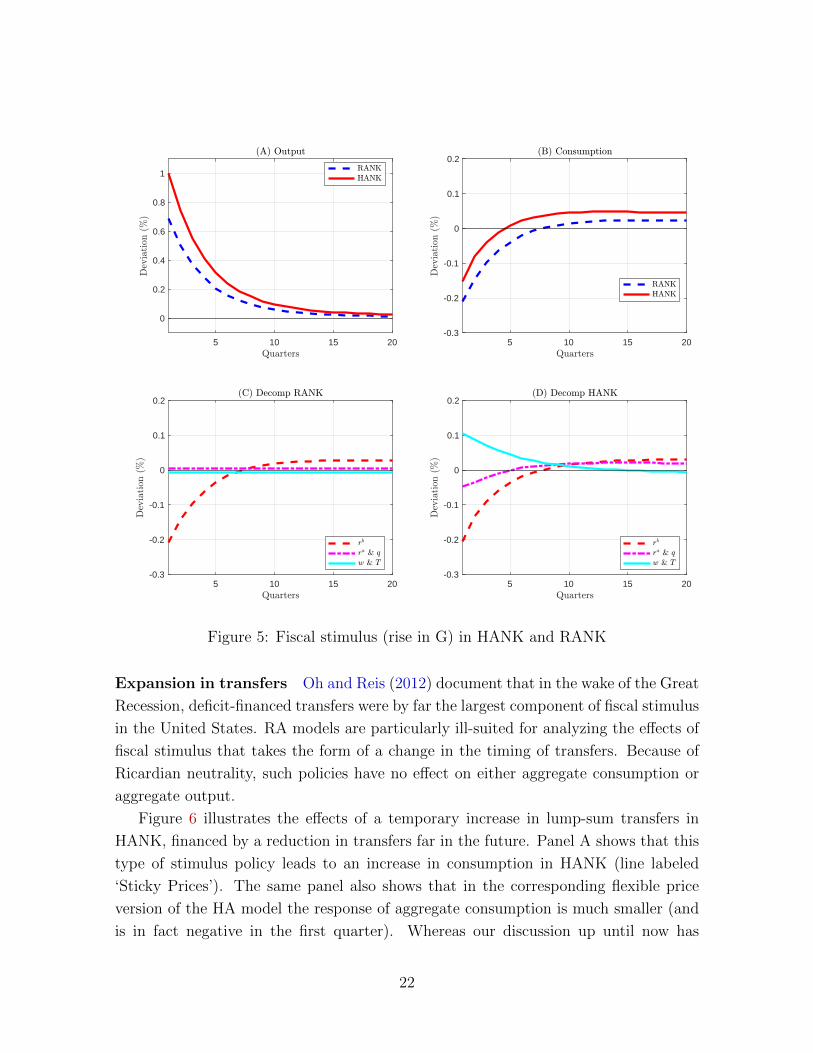
4.5 Fiscal Stimulus Shocks: Stark Non-Equivalence

Analyzing the quantitative effects of fiscal shocks has a long tradition in macroeco-

nomics. The large fiscal stimulus implemented by the governments of many developed

countries in response to the Great Recession spurred a new wave of studies that made

use of the emerging HANK framework (e.g., Oh and Reis, 2012; McKay and Reis, 2016;

Brinca et al., 2016; Hagedorn et al., 2017). In this section, we show that fiscal stim-

ulus shocks represent stark examples of non-equivalence between HANK and RANK

models.

Expansion in government spending Figure 5 illustrates the effects of a deficit-

financed temporary increase in government expenditures. The expansionary effects on

output are much stronger in HANK than in RANK (panel A) because there is less

crowding-out of private consumption (panel B). In both models, the need to finance

expenditures through a temporary rise in government debt necessitates a sufficiently

large increase in the real liquid rate in order to induce households to hold the additional

debt issued by the government. This leads to crowding-out as households lower private

consumption in response to the higher interest rates. There are two reasons why the

crowding-out is weaker in HANK than in RANK. First, we have already seen that

consumption is less sensitive to interest rates in HANK than in RANK. Second, the

increase in demand for goods by the government leads to an increase in labor demand

and hence household labor income which, by virtue of the large aggregate MPC, limits

the fall in private consumption. These differences in the transmission mechanism of

the government expenditure shock can be seen clearly in panels C and D. Once again,

it is the difference in the responsiveness of consumption to changes in income at the

household level that explains the difference between the macro dynamics in HANK and

RANK.

21

5 10 15 20

0

0.2

0.4

0.6

0.8

1

5 10 15 20-0.3

-0.2

-0.1

0

0.1

0.2

5 10 15 20-0.3

-0.2

-0.1

0

0.1

0.2

5 10 15 20-0.3

-0.2

-0.1

0

0.1

0.2

Figure 5: Fiscal stimulus (rise in G) in HANK and RANK

Expansion in transfers Oh and Reis (2012) document that in the wake of the Great

Recession, deficit-financed transfers were by far the largest component of fiscal stimulus

in the United States. RA models are particularly ill-suited for analyzing the effects of

fiscal stimulus that takes the form of a change in the timing of transfers. Because of

Ricardian neutrality, such policies have no effect on either aggregate consumption or

aggregate output.

Figure 6 illustrates the effects of a temporary increase in lump-sum transfers in

HANK, financed by a reduction in transfers far in the future. Panel A shows that this

type of stimulus policy leads to an increase in consumption in HANK (line labeled

‘Sticky Prices’). The same panel also shows that in the corresponding flexible price

version of the HA model the response of aggregate consumption is much smaller (and

is in fact negative in the first quarter). Whereas our discussion up until now has

22

2 4 6 8 10 12 14 16 18 20-0.6

-0.4

-0.2

0

0.2

0.4

0.6

0.8

-2 -1 0 1 2 3 4 5-5

0

5

10

15

20

25

30

35

Figure 6: Fiscal stimulus (rise in T). (A) IRF for aggregate consumption in HANK(B) First quarter change in consumption relative to first quarter change in lump-sumtransfers in various versions of HA models

focused on the value of introducing heterogenous households into the NK model, this

comparison highlights the role of sticky prices into HA models. Since well before the

Great Recession, HA models with incomplete markets have been used as non-Ricardian

settings in which one can study the aggregate effects of fiscal policy (e.g, Heathcote

(2005)). Introducing New Keynesian elements into HA models has broadened the set

of economic mechanisms that these analyses can capture, the most important example

being aggregate demand externalities.

In panel B of Figure 6, we show how the fraction of transfers consumed in the first

quarter varies as a function of the sizes and sign of the change in lump-sum transfers.

The black dashed line reminds us that in RANK the consumption response is always

zero. The blue dotted line shows the aggregate consumption response in partial equilib-

rium, which is simply the sum of the consumption responses of each household, holding

the wage and interest rates fixed at their steady-state levels. Note that the aggregate

MPC out of the transfer decreases as the absolute size of the transfer increases. This

is in contrast to what would be expected from a spender-saver model, as in Campbell

and Mankiw (1989). The consumption response is smaller for larger increases in trans-

fers because a larger fraction of the transfers are saved. The consumption response

is smaller for larger decreases in transfers because households become more willing to

use expensive credit to smooth consumption in the face of a temporary drop in re-

sources (recall the wedge between the interest rates on borrowing and saving). Note

also that cuts in transfers induce a stronger consumption response than the same size

increase in transfers, because of the concavity in the consumption function and the

23

kinks in household budget constraints. These predictions are in line with the evidence

discussed in Section 3.5 both qualitatively (in terms of size and sign asymmetries) and

quantitatively (in the sense that the quarterly aggregate MPC is between 15 and 25

pct).

The red solid line in panel B of Figure 6 illustrates two features of the consumption

response in the full GE model with sticky prices. First, for a wide range of values (both

negative and positive), the GE response is stronger due to the aggregate demand effects

that amplify the partial equilibrium consumption response. Second, in the presence of

an active Taylor rule for monetary policy, a very large stimulus can be so inflationary

that the monetary authority raises interest rates to a point that it overcompensates for

the expansionary effects of fiscal policy. When transfers are increased by more than

1.5% of GDP, the GE response of aggregate consumption is below the PE response.

These induced changes in the interest rate also explain the more pronounced hump-

shape relative to the PE effects. Finally, the pink dash-dot line shows that the absence

of aggregate demand effects in the flex price HA model leads to a much smaller response

of consumption for all sizes of the stimulus.

4.6 Simple Modifications to RANK

We have repeatedly seen that the key differences between HANK and RANK leading

to non-equivalence or weak equivalence are the lower sensitivity of consumption to

changes in interest rates and higher sensitivity to changes in disposable income. A

natural question that arises is whether there are simple modifications to RANK that

can replicate these features of consumption behavior, and thus generate transmission

mechanisms that are similar to those in HANK, but which avoid the computational

complexity of a full-blown heterogenous agent model.

One such modification is the Two Agent New Keynesian model (TANK) pioneered

by Bilbiie (2008) and Galı et al. (2007), which is inspired by the spender-saver model

of Campbell and Mankiw (1989). For some shocks and questions, TANK can approach

strong equivalence with HANK and thus provide a useful shortcut. For other ques-

tions, such as the consumption response to fiscal transfers of difference sizes and signs

discussed in Section 4.5, HANK and TANK provide very different answers. Kaplan et

al. (2018) and Bilbiie (2017) discuss the similarities between HANK and TANK in the

context of monetary policy shocks. In particular, Bilbiie (2017) shows that whether

the elasticity of hand-to-mouth income to aggregate income is larger or smaller than

one is a key determinant of whether the aggregate effects of a monetary shock is larger

or smaller than in RANK. Debortoli and Galı (2017) provide a detailed discussion of

the relationship between HANK and TANK in the context of additional shocks under

24

various fiscal rules. We refer the reader to these papers for more detail on TANK.

The TANK model was developed to overcome one important difference between

RANK and HANK: the absence of hand-to-mouth households and hence low aggregate

MPC in RANK. Another important difference between RANK and HANK is the nature

of household demand for liquid assets. In RANK (and also TANK) demand for liquid

assets is perfectly elastic at rb = ρ, because intertemporal substitution is the only active

savings motive. This means that, in equilibrium, the household sector is indifferent

about the level of liquid assets that it holds. A hallmark of HA models with incomplete

markets is the presence of the precautionary savings motive. This additional savings

motive means that the aggregate household demand for liquid assets in HANK is less

than perfectly elastic.

This difference in savings motives suggests that an alternative avenue for modifying

RANK is to mimic the effects of the precautionary motive by introducing an additional

savings motive directly into the utility function of the representative household. This

preference for holding safe, liquid assets captures, in a reduced-form way, the idea

that, in HANK, the household sector as a whole values the existence of a supply of

safe, liquid assets because of its precautionary value (see, e.g. Aiyagari and McGrattan

(1998)). For example, one can introduce an additional term into the utility function,

as in

u (C,H,B) = logC − ψ H1+1/ε

1 + 1/ε+ ϕ

B1−σ − 1

1− σ, (7)

where B is the quantity of real government bonds held by the representative household.

The RANK model with bonds in the utility function is closer to HANK in several

important dimensions. First, the additional term in the utility function introduces a

wedge that drives the steady-state liquid interest rate rb below the illiquid interest rate

ra, as in HANK.11 This wedge is governed by the level parameter ϕ, so can be chosen

so that both steady-state returns are the same in both HANK and RANK. Second,

in the neighborhood of the steady-state, the curvature parameter σ governs both the

sensitivity of consumption to interest rates and income. Higher values of σ lead to a

larger aggregate MPC and lower sensitivity to changes in the interest rate. Intuitively,

when σ is large, the marginal utility of savings decreases quickly so the household

desires to consume more out of a transitory increase in income. For example, we have

found that setting σ = 2.5 yields an aggregate MPC of similar magnitude as in HANK

and an IRF decomposition in response to a TFP shock that is very similar to the

11 Without liquid assets in the utility function, the RANK model has ra ≤ rb in the steady-state.In our baseline version of RANK, ra < rb because of the negative dependence of the transaction costfunction χ(d, a) on a. If the transaction cost were a function only of d (or were not present at all)then we would have ra = rb in the steady-state of RANK.

25

decomposition in HANK.

Finally, recent work by Hagedorn (2018) has shown that the class of fiscal and

monetary policy rules that lead to determinacy is much larger in HANK than in RANK.

The determinacy properties of the RANK model with bonds in the utility function are

very similar to those in HANK in this respect (Hagedorn, 2018; Michaillat and Saez,

2018). The reason, which is closely related to arguments in Epstein and Hynes (1983),

is precisely that in both HANK and the modified RANK model, the household sector

is not indifferent about the path of the supply of real bonds.

5 Macro Questions that Require a Model with Heterogeneity

So far, we have addressed macroeconomic questions about impulses and propagation

that are well-posed in both HA and RA models. However, some important questions

pertaining to macroeconomic dynamics can only be addressed in models with household

heterogeneity. In this section, we provide three examples. First, we analyze two types of

aggregate shocks that are not well-defined in RA models. Second, we show how different

responses to aggregate shocks by households at different parts of the distribution can

aid in the identification of shocks and transmission mechanisms. Third, we illustrate

how HA models can be used to assess the impact of aggregate shocks on household

inequality.

5.1 Microfoundation for a Fall in Aggregate Demand

Two salient features of the Great Recession were a deep and prolonged drop in aggregate

expenditures and a simultaneous sharp fall in the natural interest rate which led to

a binding ZLB. These features of the data are consistent with a drop in aggregate

demand as a primary driving force behind the recession. Yet, in order to generate

a large sudden fall in aggregate demand in RANK models, most researchers have

resorted to assuming a shock to the discount factor of the representative household.

Macroeconomists often justify this shock as a stand-in for some unspecified deeper

shock that acts as if ‘households become more patient’ (Eggertsson and Krugman,

2012). We examined this type of discount factor shock in HANK and RANK in Section

4.2.

HANK models offer the possibility to generate a fall in aggregate demand through

shocks that strengthen households’ desire to save due to mechanisms that are both

more deeply micro-founded and are consistent with aspects of the micro data. Two

leading examples are (i) tighter credit limits (as in Guerrieri and Lorenzoni, 2017) that

reduce borrowing capacity, leading constrained households to deleverage sharply and

26

5 10 15 20-0.6

-0.5

-0.4

-0.3

-0.2

-0.1

0

0.1

5 10 15 20-0.6

-0.5

-0.4

-0.3

-0.2

-0.1

0

0.1

5 10 15 20-0.5

0

0.5

1

1.5

2

5 10 15 20-2

-1

0

1

2

Figure 7: Microfoundations for demand shock in HANK

unconstrained households to increase their savings in order to avoid the possibility of

being constrained in the future; and (ii) increased uninsurable labor market risk (as in

Den Haan et al., 2017; Bayer et al., 2017) that exacerbates the desire for precautionary

saving.12

For both of these shocks, the two-asset version of HANK offers an advantage over

the one-asset version in generating the desired fall in aggregate demand. The additional

household savings are channeled towards the liquid asset, which is the better asset for

consumption smoothing purposes, rather than towards productive capital, which would

be expansionary because of a counterfactual investment boom.13

Figure 7 illustrates the dynamics of aggregate consumption and interest rates in

12In certain models that admit aggregation in closed form, it is even possible to show that a rise inidiosyncratic uncertainty is mathematically equivalent to a rise in the discount factor of the pseudo-representative agent (Braun and Nakajima, 2012; Werning, 2015).

13Indeed for this reason the literature that studies these shocks in one-asset HANK models typicallyabstracts from productive investment.

27

0 20 40 60 80 100

0

0.2

0.4

0.6

0.8

1

0 10 20 30 40 50 60 70 80 90 100

0

0.1

0.2

0.3

0.4

0.5

0.6

0.7

0.8

0.9

1

Figure 8: Transmission mechanim of a monetary shock across the distribution of liquidwealth. Panel (A) total effect. Panel (B) decomposition.

response to these two shocks in our version of HANK. Panels A and B show that the

shocks generate a much larger fall in aggregate demand with sticky prices than with

flexible prices, precisely because of the aggregate demand channel, which is substantial

because of the high MPC households. Panels C and D show that both the real and the

nominal liquid interest rates fall, and that the size of the drop in the nominal rate can

easily be large enough to hit the ZLB.14

5.2 Heterogeneity in the Transmission Mechanism

Weakly equivalent models differ in terms of their transmission mechanism, but not in

terms of their aggregate response to a shock. Hence, collecting empirical evidence on

transmission mechanisms is a crucial step in distinguishing different models. But trying

to uncover mechanisms from time-series data alone is extremely challenging, because

time is the only source of variation and confounding factors abound. As discussed

by Nakamura and Steinsson (2018), cross-sectional responses are often a much more

powerful diagnostic tool. One advantage of HA models is that they make explicit

predictions about how the impact of an aggregate shock varies across the distribution

of households. One can therefore exploit richer micro data to gather support for a

specific model or mechanism.

In Figure 8, we show how the initial drop in consumption in response to the mone-

tary shock in HANK varies across the distribution of liquid wealth (panel A), together

14We model the increase in uninsurable productivity risk as a mean-preserving spread in the pro-ductivity distribution. As in Bayer et al. (2017), we make an offsetting adjustment to preferences sothat this does not lead to a mechanical increase in aggregate labor supply. We model tighter credit asan increase in the financial intermediation wedge between the interest rates on saving and borrowing.

28

with the IRF decomposition at each point in the distribution (panel B). The consump-

tion drop is largest for the mass of households with zero liquid wealth (the flat section

of the plots) and is almost entirely due to the general equilibrium drop in labor income.

These hand-to-mouth households have high MPCs and low sensitivity to interest rates.

For households with positive liquid wealth (those above the 35th percentile), the direct

effects of the interest rate change is larger than the indirect effect from the fall in labor

income, because these households have low MPCs. Moving further up the wealth dis-

tribution, the consumption response gradually increases because the substitution effect

becomes stronger as it becomes less likely that households will be hand-to-mouth in the

future. However, at the very top of the distribution, the consumption response starts

to fall because the positive income effect from the increase in the interest rate becomes

strong enough to mute the drop in consumption. Ongoing empirical work using house-

hold panel data on consumption, income, and wealth provides some support for this

pattern of cross-sectional transmission mechanism (see, e.g., Cloyne et al., 2017).

Examining consumption responses at different points in the wealth distribution

is also potentially informative for distinguishing between different types of aggregate

shocks. For example, in Section 5.1 we showed that three different aggregate shocks

(discount factor, credit tightness, income risk) all produce qualitatively similar aggre-

gate dynamics – a large fall in aggregate demand that leads to a decline in interest

rates. However, it turns out that the distributional response of these three shocks is

very different. For example, the discount factor shock generates consumption responses

that are much more evenly distributed across the liquid wealth distribution than the

credit and risk shocks, and the fall in consumption in response to the credit shock is

more concentrated among households with negative liquid wealth than in response to

the risk shock. We think that using the disaggregated response of aggregate shocks

across the distribution of households in this way is an extremely promising avenue for

using HA models to help identify the underlying sources of aggregate fluctuations.

These stark differences in the consumption response across the wealth distribution

and across alternative micro-foundations for an aggregate demand shock are illustrated

in Figure 9. For each shock, the response at each point in the liquid wealth distribution

is displayed as a multiple of the average consumption response in the population. This

means that if all households respond in approximately the the same way, the plot would

be close to a horizontal line at 1, as is the case for the preference shock (red dash-dot

line). For the productivity shock (black dashed line), the response is highest for the

hand-to-mouth households with zero liquid wealth. For the credit shocks (blue solid

line) the response is only substantially different from the average for households who

are on or close to the borrowing constraint.

29

0 20 40 60 80 100-2

0

2

4

6

8

10

Figure 9: Relative consumption response at different points in liquid wealth distributionfor three different shocks in HANK.

5.3 Impact of Aggregate Shocks on Inequality

HA models are not only useful for understanding how wealth and income inequality

can affect the magnitude and transmission mechanism of aggregate shocks. The value

of HA models arise also when the question is turned on its head: to what extent do

macroeconomic shocks affect the level and shape of inequality?

As an example, we analyze how a contractionary monetary shock affects the distri-

bution of consumption in the two-asset HANK model. Although the primary objective

of central banks is maintaining price stability, whereas the mandate for redistribution

lies mostly with fiscal policymakers, it is nonetheless useful for central banks to also

consider the distributional consequences of monetary policy, for at least two reasons.

First, against a backdrop of of rising inequality, central banks’ actions are being scru-

tinized more and more closely. Second, by affecting the wealth distribution central

banks can alter the transmission mechanism for both monetary policy itself, and other

shocks.

Figure 10 shows that a contractionary monetary policy shock increases consumption

inequality. The rise in the interest rate favors the very wealthy households through

a positive income effect, as by the consumption of the top 1 percent of the wealth

distribution (red dashed line). The fall in aggregate demand caused by the monetary

tightening leads to a reduction in labor income, which affects consumption most sharply

for households towards the bottom of the distribution. This can be seen by comparing

the consumption drop for households in the top 25 percent of the distribution (solid

30

2 4 6 8 10 12 14 16 18 20-0.7

-0.6

-0.5

-0.4

-0.3

-0.2

-0.1

0

0.1

Figure 10: Response of different percentiles of the consumption distribution to a con-tractionary monetary shock in HANK

pink line) with the corresponding drop for households in the bottom 25 percent of the

distribution (dash-dot blue line).

Overall, our model suggests only a modest impact of monetary policy on inequality,

especially when compared to the trends observed over the past several decades. The

empirical analysis in Coibion et al. (2017) finds some support to the conclusion that

contractionary monetary policy has a positive, but small, effect on inequality.

6 Conclusions: Looking Ahead

A new macroeconomic framework is emerging. It embeds a rich representation of

household consumption and portfolio choices, consistent with many aspects of microe-

conomic data, into a dynamic general equilibrium model of the macroeconomy that

can accommodate a wide range of aggregate shocks and demand-side effects. This

framework is appealing because it offers a coherent way to study questions that per-

tain to cross-sectional inequality, economic mobility, social insurance and redistributive

policies in conjunction with questions that pertain to the dynamics of macroeconomic

variables, propagation mechanisms of aggregate shocks, and stabilization policies. But,

to restate the question we posed in the Introduction: does microeconomic household

heterogeneity interact with macroeconomic shocks in interesting, and quantitatively

relevant, ways? Does it change the answers offered by RA models? And, does it allow

us to address a wider range of macro questions?

We proposed a set of criteria to determine whether HA models are equivalent to

31

RA models and showed, through a series of examples, that the extent of equivalence

(strong, weak, none) differs across shocks. We argued that incorporating heterogeneity

often entirely changes the transmission mechanism of the shock. For example, in

HANK models the response of aggregate consumption depends more on the dynamics

of labor income and less on the dynamics of interest rates. And in HANK models, fiscal

stimulus is more powerful, and monetary policy is less powerful than in RANK. We

suggested a simple modification to RANK – introducing a direct preference for holding

safe, liquid real assets into the utility function of the representative household – that

can bring many of the properties of RANK in closer alignment with those of HANK.

HANK models also allow us to analyze new aggregate shocks where cross-sectional

heterogeneity is crucial – such as a tightening of credit or an increase in idiosyncratic

labor market risk – that can shed light on the Great Recession. Finally, within this

class of model one can study the implications of macro shocks and macro policies for

income and wealth inequality.

The HANK framework is still in its infancy. In what follows, we outline seven

promising directions where these models are being further developed.

Other sources of aggregate demand effects and monetary non-neutrality.

The HANK framework that we outlined borrows its production side from the textbook

New Keynesian model. As such, aggregate demand and monetary shocks have real

effects because firms face adjustment costs when changing prices. Although there is

vast microeconomic evidence for price stickiness (Nakamura and Steinsson, 2013), the

jury is still out over whether this alone accounts for the large real effects of monetary

policy shocks and fluctuations in aggregate demand. Moreover, there is much less mi-

croeconomic evidence for the large movements in quantities implied by price stickiness

in the NK model.

Nominal and real wage rigidity have been suggested as alternative explanations.

On the measurement side, the estimation of individual wage rigidity for new hires and

incumbents remains limited by a lack of representative high-frequency data on earnings

and hours (see Hurst et al., 2017, for recent progress). On the theoretical side, a micro-

foundation of wage rigidity requires modeling labor market frictions, a point which we

discuss below.15

A promising alternative approach to generating real effects of changes in aggregate

demand, that does not rely on price stickiness, is through real frictions in the product

market (Huo and Rıos-Rull, 2016; Kaplan and Menzio, 2016). A common feature of

15Within RANK models, recent progress in this direction has been made by Gertler and Trigari(2009) and Christiano et al. (2016)

32

these models is the existence of search frictions in product markets. Households vary

the extent to which they hunt for bargains based on their wealth, income and demand

for consumption, which in turn affects the hiring decisions of firms. In Huo and Rıos-

Rull (2016) this shows up as endogenous movements in aggregate productivity while in

Kaplan and Menzio (2016) it shows up as endogenous movements in the competitiveness

of product markets and markups. In both cases, changes in aggregate demand lead

to changes labor demand. Models with these types of frictional product markets fit

particularly well with HA models because household shopping behavior is intimately

linked to consumption decisions.

Labor market frictions and micro-foundation of labor income risk. There

are several reasons why it may be useful to enrich the model of the labor market in

HANK models. First, the bilateral monopoly that emerges in many frictional labor

markets implies that wages may fluctuate less than labor productivity. For example,

if wage renegotiation occurs only when it is mutually beneficial (Postel-Vinay and

Robin, 2002), wages might even be completely insensitive to aggregate shocks, within

existing jobs (Hall and Milgrom, 2008). On the other hand, labor market tightness,

job separations and movements along the job ladder are endogenous and responsive to

aggregate shocks. Thus, labor market frictions provide a way to endogenize the extent

and nature of idiosyncratic labor market risk. The fact that labor market risk is mostly

exogenous in current HANK models is a gaping whole in the framework.16

Second, as recently emphasized by Moscarini and Postel-Vinay (2017), combining

the basic equilibrium-search sequential-auction model with a New Keynesian produc-

tion block leads to the emergence of endogenous markup shocks. These occur when a

firm chooses to match an outside offer to one of its workers, in which case the wage

goes up without any change in productivity. Embedding this mechanism into HANK

would then generate a credible micro-foundation for both of the two key driving forces

behind inflation dynamics: (i) aggregate demand shocks, which are driven by the dis-

tribution of MPCs in the population; and (ii) cost-push shocks, which are driven by

the distribution of workers along the job ladder.

Gross and nominal asset positions. In the HANK model outlined in Section 3,

household portfolios are composed of two real assets: a net liquid asset (e.g., bank

accounts net of credit card debt) and a net illiquid asset (e.g., housing net of mort-

gages). Relative to household-level data, there are two major limitations of this balance

16Hubmer (2018), for example, shows that skewness and kurtosis in earnings growth uncovered inmicro data (Guvenen et al., 2015; Arellano et al., 2017) arise endogenously in a canonical frictionalmodel of the labor market with on-the-job search.

33

sheet. First, many households hold highly leveraged positions, particularly in terms of

housing. Accommodating leveraged portfolios in HANK would require keeping track

of gross positions, which poses computational challenges because of the additional in-

dividual state variables that are introduced. Nonetheless, this extension is potentially

important. For example, when mortgage contracts allow some degree of pass-through

of interest rates (because of adjustable rates or the option to refinance as in, e.g. Wong

(2015) ), changes in interest rates can have significant cash-flow effects on expenditures

for borrowers, as in the data (e.g. Floden et al., 2016; Di Maggio et al., 2017; Kaplan

and La Cava, 2017). Hedlund et al. (2017) make progress in this direction.

Second, many assets and liabilities (e.g., cash, bank accounts, government bonds,

mortgage debt) earn nominal returns that do not adjust instantaneously to aggregate

conditions. As a result, surprise inflation can have redistributive effects (Doepke and

Schneider, 2006; Auclert, 2017) that our model specification misses entirely.

Finally, in a version of the model with endogenous unsecured or secured credit limits

(e.g. Chatterjee et al., 2007; Favilukis et al., 2017), aggregate shocks can transmit to

the real economy also by modifying the extent of credit availability. Recent studies

by Agarwal et al. (2015) and Gross et al. (2016) estimate a sizable MPC out of the

additional liquidity provided by changes in credit limits.

Time-varying risk premia. The asset pricing implications of this first generation

of HANK models are disconcerting. Equity prices barely move in response to aggregate

shocks, and when they do, it is often in the wrong direction. For example, expansionary

monetary policy shocks increase marginal costs and reduce profits for intermediate

producers, leading to a fall in the price of equity. Although the evidence on the co-

movement between asset prices and monetary policy is somewhat mixed, it mostly

points towards stock and house prices rising in response to expansionary monetary

policy.

A large literature in finance concludes that the most promising way to generate

asset prices movements in response to macroeconomic fluctuations is through time-

varying risk premia. For example, as explained by Cochrane (2017), successful asset

pricing models all reflect the idea that market participants’ willingness to bear risk is

greater in booms than in recessions.

Why is it important to generate realistic asset price movements in HANK? The main

reason is that heterogeneity in household balance sheets means that some households

are much more exposed to movements in asset prices than others (Glover et al., 2017).

The current versions of HANK miss the potentially large wealth effects on consumption

for wealthy households that can arise from changes in asset prices.

34

Financial intermediaries. As of now there are no banks in HANK. In the version

of HANK that we presented, all liquid assets are provided by the fiscal authority and

are fully backed by future tax revenues. Thus there is no scope for money creation

and any changes in households’ demand to save in liquid assets directly affects the

government budget constraint. This induces a stronger link between fiscal policy and

household savings behavior than in reality, exactly because of the lack of a banking

sector. For the reasons we described in Section 4.6, this is particularly important in

HANK because the household sector is not indifferent over the quantity of liquid assets

available for savings.

Moreover, many of the prevailing accounts of the Great Recession attribute a central

role to the deterioration of banks’ balance sheets. Exploring this propagation mecha-

nism requires an explicit model of the banking sector, along with regulatory constraints

on their balance sheets.

As is illustrated in Kaplan et al. (2016), the two-asset HANK model lends itself nat-

urally to the introduction of banks, since one of the key role of financial intermediaries

is precisely that of liquidity transformation.

Deviations from rational expectations and complete information. The HANK

model has so far developed under the assumptions of rational expectations and com-

plete information. Some recent papers have showed how dispersed information (An-

geletos and Lian, 2017) or behavioral phenomena (Farhi and Werning, 2017) can have

drastic consequences for the relative strengths of partial equilibrium versus general

equilibrium affects of aggregate shocks, thus changing the incidence of the shock across

the household distribution.

Optimal policy. In HA models with incomplete markets and aggregate shocks, sta-

bilization policy has also redistributive and social insurance implications. Hence the

design of optimal policy is altered by these considerations. For example, McKay and

Reis (2016) show that removing automatic fiscal stabilizers would not amplify aggre-

gate consumption fluctuations as long as monetary policy follows a standard Taylor

rule, but would lead to large welfare costs because of the decrease in social insurance.

Gornemann et al. (2016) argue that a monetary policy rule that emphasizes price sta-

bility redistributes towards rich households, while one that stresses output stability

redistributes towards poor households who are more exposed to unemployment risk,

and that the median household prefers output stability. Finally, there is an emerging

literature that uses a Ramsey approach to characterize optimal policies in this class

of models. Computationally, this is a challenging problem, but recent advances have

35

been made by Le Grand and Ragot (2017), Nuno and Thomas (2017) and Bhandari et

al. (2017).

36

References

Acharya, Sushant and Keshav Dogra, “Understanding HANK: Insights from a

PRANK,” Technical Report, Federal Reserve Bank of New York 2018.

Achdou, Yves, Jiequn Han, Jean-Michel Lasry, Pierre-Louis Lions, and Ben-

jamin Moll, “Income and Wealth Distribution in Macroeconomics: A Continuous-Time

Approach,” Working Paper 23732, National Bureau of Economic Research 2017.

Agarwal, Sumit, Souphala Chomsisengphet, Neale Mahoney, and Johannes

Stroebel, “Regulating Consumer Financial Products: Evidence from Credit Cards,” The

Quarterly Journal of Economics, 2015, 130 (1), 111–164.

Ahn, SeHyoun, Greg Kaplan, Benjamin Moll, Thomas Winberry, and Christian

Wolf, “When Inequality Matters for Macro and Macro Matters for Inequality,” in “NBER

Macroeconomics Annual 2017, volume 32,” University of Chicago Press, 2017.

Aiyagari, Rao, “Uninsured Idiosyncratic Risk and Aggregate Saving,” The Quarterly Jour-

nal of Economics, 1994, 109 (3), 659–684.

Aiyagari, S Rao and Ellen R McGrattan, “The Optimum Quantity of Debt,” Journal

of Monetary Economics, 1998, 42 (3), 447–469.

Angeletos, George-Marios and Chen Lian, “Dampening General Equilibrium: From

Micro to Macro,” Working Paper, National Bureau of Economic Research 2017.

Arellano, Manuel, Richard Blundell, and Stephane Bonhomme, “Earnings and Con-

sumption Dynamics: A Nonlinear Panel Data Framework,” Econometrica, 2017, 85 (3),

693–734.

Attanasio, Orazio and Steven J. Davis, “Relative Wage Movements and the Distribution

of Consumption,” Journal of Political Economy, 1996, 104 (6), 1227–1262.

Auclert, Adrien, “Monetary Policy and the Redistribution Channel,” Working Paper

23451, National Bureau of Economic Research 2017.

Baker, Scott, “Debt and the Response to Household Income Shocks: Validation and Ap-

plication of Linked Financial Account Data,” Journal of Political Economy, 2018, (forth-

coming).

Bayer, Christian, Ralph Lutticke, Lien Pham-Dao, and Volker Tjaden, “Precau-

tioary Savings, Illiquid Assets, and the Aggregate Consequences of Shocks to Household

Income Risk,” Working Paper, University of Bonn 2017.

37

Benhabib, Jess and Alberto Bisin, “Skewed Wealth Distributions: Theory and Empir-

ics,” Journal of Economic Literature, 2016, (forthcoming).

Bewley, Truman, “A Difficulty with the Optimum Quantity of Money,” Econometrica,

1983, 51 (5), 1485–1504.

Bhandari, Anmol, David Evans, Mikhail Golosov, and Thomas J Sargent, “In-

equality, Business Cycles and Monetary-Fiscal,” Working Paper, University of Minnesota

2017.

Bilbiie, Florin O, “Limited Asset Markets Participation, Monetary Policy and (inverted)

Aggregate Demand Logic,” Journal of Economic Theory, 2008, 140 (1), 162–196.

, “The New Keynesian Cross: Understanding Monetary Policy with Hand-to-Mouth House-

holds,” Technical Report, Working Paper, PSE 2017.

Blundell, Richard, Luigi Pistaferri, and Ian Preston, “Consumption Inequality and

Partial Insurance,” American Economic Review, 2008, 98 (5), 1887–1921.

Boppart, Timo, Per Krusell, and Kurt Mitman, “Exploiting MIT Shocks in

Heterogeneous-Agent Economies: The Impulse Response as a Numerical Derivative,”

Working Paper, National Bureau of Economic Research 2017.

Braun, R Anton and Tomoyuki Nakajima, “Uninsured countercyclical risk: an aggrega-

tion result and application to optimal monetary policy,” Journal of the European Economic

Association, 2012, 10 (6), 1450–1474.

Brinca, Pedro, Hans A Holter, Per Krusell, and Laurence Malafry, “Fiscal Multi-

pliers in the 21st Century,” Journal of Monetary Economics, 2016, 77, 53–69.

Broda, Christian and Jonathan A Parker, “The Economic Stimulus Payments of 2008

and the Aggregate Demand for Consumption,” Journal of Monetary Economics, 2014, 68

(S), 20–36.

Broer, Tobias, Niels-Jakob H Hansen, Per Krusell, and Erik Oberg, “The New

Keynesian Transmission Mechanism: A Heterogenous-Agent Perspective,” Working Paper,

National Bureau of Economic Research 2016.

Browning, Martin and Thomas F Crossley, “The Life-Cycle Model of Consumption

and Saving,” Journal of Economic Perspectives, 2001, 15 (3), 3–22.

Brumm, Johannes and Simon Scheidegger, “Using Adaptive Sparse Grids to Solve

High-Dimensional Dynamic Models,” Econometrica, 2017, 85 (5), 1575–1612.

38

Caballero, Ricardo, “Aggregate Investment, Chapter 12 in JB Taylor and M. Woodford

(eds) Handbook of Macroeconomics, Volume 1B,” 1999.

Campbell, John Y and N Gregory Mankiw, “Consumption, Income and Interest Rates:

Reinterpreting the Time Series Evidence,” in “NBER Macroeconomics Annual,” Vol. 4 of

NBER Chapters, National Bureau of Economic Research, 1989, pp. 185–246.

Canzoneri, Matthew B, Robert E Cumby, and Behzad T Diba, “Euler Equations

and Money Market Interest Rates: A Challenge for Monetary Policy Models,” Journal of

Monetary Economics, oct 2007, 54 (7), 1863–1881.

Carroll, Christopher D, “Buffer-Stock Saving and the Life Cycle/Permanent Income Hy-

pothesis,” The Quarterly Journal of Economics, 1997, 112 (1), 1–55.

Carroll, Christopher, Jiri Slacalek, Kiichi Tokuoka, and Matthew N. White,

“The Distribution of Wealth and the Marginal Propensity to Consume,” Quantitative

Economics, 2017, 8 (3), 977–1020.

Chatterjee, Satyajit, Dean Corbae, Makoto Nakajima, and Jose-Vıctor Rıos-Rull,

“A Quantitative Theory of Unsecured Consumer Credit with Risk of Default,” Economet-

rica, 2007, 75 (6), 1525–1589.

Christelis, Dimitris, Dimitris Georgarakos, Tullio Jappelli, Luigi Pistaferri, and

Maarten van Rooij, “Asymmetric Consumption Effects of Transitory Income Shocks,”

Working Paper 467, Centre for Studies in Economics and Finance (CSEF) 2017.

Christiano, Lawrence J., Martin S. Eichenbaum, and Mathias Trabandt, “Unem-

ployment and Business Cycles,” Econometrica, 2016, 84 (4), 1523–1569.

Clarida, Richard, Jordi Gali, and Mark Gertler, “The Science of Monetary Policy: A

New Keynesian Perspective,” Journal of Economic Literature, dec 1999, 37 (4), 1661–1707.

Cloyne, James, Clodomiro Ferreira, and Paolo Surico, “Monetary Policy When

Households Have Debt: New Evidence on the Transmission Mechanism,” Working Pa-

per, London Business School 2017.

Cochrane, John, “Whither Inflation,” Blog Post 2015.

Cochrane, John H, “A Simple Test of Consumption Insurance,” Journal of Political Econ-

omy, 1991, 99 (5), 957–976.

, “Macro-Finance,” Review of Finance, 2017, 21 (3), 945–985.

39

Coibion, Olivier, Yuriy Gorodnichenko, Lorenz Kueng, and John Silvia, “Innocent

Bystanders? Monetary policy and inequality,” Journal of Monetary Economics, 2017, 88,

70–89.

De Nardi, Mariacristina and Giulio Fella, “Saving and Wealth Inequality,” Review of

Economic Dynamics, 2017, 26, 280–300.

Deaton, Angus, “Life-cycle Models of Consumption: Is the Evidence Consistent with the

Theory?,” in “Advances in Econometrics: Volume 2: Fifth World Congress,” Vol. 2 Cam-

bridge University Press 1987, p. 121.

Debortoli, Davide and Jordi Galı, “Monetary Policy with Heterogeneous Agents: In-

sights from TANK Models,” Technical Report, mimeo 2017.

Den Haan, Wouter J, Pontus Rendahl, and Markus Riegler, “Unemployment (Fears)

and Deflationary Spirals,” Centre for Economic Policy Research (CEPR) Discussion Paper

Series, 2017, (10814).

Di Maggio, Marco, Amir Kermani, Benjamin J. Keys, Tomasz Piskorski, Rodney

Ramcharan, Amit Seru, and Vincent Yao, “Interest Rate Pass-Through: Mortgage

Rates, Household Consumption, and Voluntary Deleveraging,” American Economic Re-

view, 2017, 107 (11), 3550–3588.

Doepke, Matthias and Martin Schneider, “Inflation and the Redistribution of Nominal

Wealth,” Journal of Political Economy, 2006, 114 (6), 1069–1097.

Duarte, Victor, “Machine Learning for Continuous-Time Economics,” Working Paper, MIT

2018.

Eggertsson, Gauti B and Paul Krugman, “Debt, Deleveraging, and the Liquidity Trap:

A Fisher-Minsky-Koo Approach,” The Quarterly Journal of Economics, 2012, 127 (3),

1469–1513.

Epstein, Larry G and J Allan Hynes, “The rate of time preference and dynamic economic

analysis,” Journal of Political Economy, 1983, 91 (4), 611–635.

Fagereng, Andreas, Martin Holm, and Gisle Natvik, “MPC Heterogeneity and House-

hold Balance Sheets,” Discussion Paper 852, Statistics Norway 2016.

Farhi, Emmanuel and Ivan Werning, “Monetary Policy, Bounded Rationality, and In-

complete Markets,” Working Paper, National Bureau of Economic Research 2017.

40

Favilukis, Jack, Sydney C. Ludvigson, and Stijn Van Nieuwerburgh, “The Macroe-

conomic Effects of Housing Wealth, Housing Finance, and Limited Risk Sharing in General

Equilibrium,” Journal of Political Economy, 2017, 125 (1), 140–223.

Fernandez-Villaverde, Jesus, Samuel Hurtado, and Galo Nuno, “Financial Frictions

and the Wealth Distribution,” Manuscript, 2018.

Floden, Martin, Matilda Kilstrom, Josef Sigurdsson, and Roine Vestman, “House-

hold Debt and Monetary Policy: Revealing the Cash-Flow Channel,” Working Paper,

Stockholm University 2016.

Fuster, Andreas, Greg Kaplan, and Basit Zafar, “What Would You do With $500?

Evidence from Gains, Losses, News, and Loans,” Working Paper, University of Chicago

2018.

Gali, Jordi, “Technology, Employment, and the Business Cycle: Do Technology Shocks

Explain Aggregate Fluctuations?,” American Economic Review, 1999, 89 (1), 249–271.

Galı, Jordi, J David Lopez-Salido, and Javier Valles, “Understanding the effects of

government spending on consumption,” Journal of the European Economic Association,

2007, 5 (1), 227–270.

Gertler, Mark and Antonella Trigari, “Unemployment Fluctuations with Staggered

Nash Wage Bargaining,” Journal of Political Economy, 2009, 117 (1), 38–86.

and Simon Gilchrist, “Monetary Policy, Business Cycles, and the Behavior of Small

Manufacturing Firms,” The Quarterly Journal of Economics, 1994, 109 (2), 309–340.

and , “What Happened: Financial Factors in the Great Recession,” Working Paper,

New York University 2017.

Glover, Andrew, Jonathan Heathcote, Dirk Krueger, and Jose-Vıctor Rıos-Rull,

“Intergenerational Redistribution in the Great Recession,” Working Paper, University of

Texas 2017.

Gornemann, Nils, Keith Kuester, and Makoto Nakajima, “Doves for the Rich, Hawks

for the Poor? Distributional Consequences of Monetary Policy,” Working Paper, Federal

Reserve Bank of Philadelphia 2016.

Gross, Tal, Matthew J. Notowidigdo, and Jialan Wang, “The Marginal Propensity to

Consume over the Business Cycle,” Working Paper 22518, National Bureau of Economic

Research 2016.

41

Guerrieri, Veronica and Guido Lorenzoni, “Credit Crises, Precautionary Savings, and

the Liquidity Trap,” Quarterly Journal of Economics, 2017, 132 (3), 1427–1467.

Guvenen, Fatih, “Macroeconomics with Heterogeneity: A Practical Guide,” FRB of Rich-

mond Economic Quarterly, 2011, 97 (3), 255–326.

, Fatih Karahan, Serdar Ozkan, and Jae Song, “What Do Data on Millions of U.S.

Workers Reveal about Life-Cycle Earnings Risk?,” Working Paper 20913, National Bureau

of Economic Research 2015.

Hagedorn, Marcus, “Prices and Inflation when Government Bonds are Net Wealth,” Tech-

nical Report, University of Oslo 2018.

, Iourii Manovskii, and Kurt Mitman, “The Fiscal Multiplier,” Working Paper, Uni-

versity of Oslo 2017.

Hall, Robert, “Stochastic Implications of the Life Cycle-Permanent Income Hypothesis:

Theory and Evidence,” Journal of Political Economy, 1978, 86 (6), 971–987.

Hall, Robert E and Paul R Milgrom, “The limited influence of unemployment on the

wage bargain,” The American Economic Review, 2008, 98 (4), 1653–1674.

Heathcote, Jonathan, “Fiscal Policy with Heterogeneous Agents and Incomplete Markets,”

The Review of Economic Studies, 2005, 72 (1), 161–188.

, Kjetil Storesletten, and Giovanni L. Violante, “Quantitative Macroeconomics with

Heterogeneous Households,” Annual Review of Economics, 2009, 1 (1), 319–354.

, , and Giovanni L Violante, “Consumption and Labor Supply with Partial Insurance:

An Analytical Framework,” American Economic Review, 2014, 104 (7), 2075–2126.

Hedlund, Aaron, Fatih Karahan, Kurt Mitman, and Serdar Ozkan, “Monetary

Policy, Heterogeneity, and the Housing Channel,” Working Paper, University of Missouri

2017.

Hubmer, Joachim, “The Job Ladder and its Implications for Earnings Risk,” Review of

Economic Dynamics, 2018, (forthcoming).

Huggett, Mark, “The Risk-Free Rate in Heterogeneous-Agent Incomplete-Insurance

Economies,” Journal of Economic Dynamics and Control, 1993, 17 (5-6), 953–969.

Huo, Zhen and Jose Vıctor Rıos-Rull, “Financial Frictions, Asset Prices, and the Great

Recession,” Working Paper, CEPR Discussion Papers 2016.

42

Hurst, Erik, John Grigsby, and Ahu Yildirmaz, “Wage Stickiness During the Great

Recession,” Technical Report, The University of Chicago Booth School of Business 2017.

Imrohorolu, Aye, “Cost of Business Cycles with Indivisibilities and Liquidity Constraints,”

Journal of Political Economy, 1989, 97, 1364–1383.

Jappelli, Tullio and Luigi Pistaferri, “The Consumption Response to Income Changes,”

Annual Review of Economics, 2010, 2 (1), 479–506.

Johnson, David S, Jonathan A Parker, and Nicholas S Souleles, “Household Expen-

diture and the Income Tax Rebates of 2001,” American Economic Review, 2006, 96 (5),

1589–1610.

Kaplan, Greg and Gianni La Cava, “The Household Cash Flow Channel of Monetary

Policy: Evidence from Australia,” 2017.

and Giovanni L. Violante, “A Model of the Consumption Response to Fiscal Stimulus

Payments,” Econometrica, jul 2014, 82 (4), 1199–1239.

and Guido Menzio, “Shopping Externalities and Self-Fulfilling Unemployment Fluctu-

ations,” Journal of Political Economy, jun 2016, 124 (3), 771–825.

, Benjamin Moll, and Giovanni L Violante, “A Note on Unconventional Monetary

Policy in HANK,” Technical Report, Princeton University 2016.

, , and , “Monetary Policy According to HANK,” American Economic Review, 2018,

(forthcoming).

, Gianluca Violante, and Justin Weidner, “The Wealthy Hand-to-Mouth,” Brookings

Papers on Economic Activity, 2014, (1), 77–138.

Khan, Aubhik and Julia K Thomas, “Idiosyncratic Shocks and the Role of Nonconvex-

ities in Plant and Aggregate Investment Dynamics,” Econometrica, 2008, 76 (2), 395–436.

Krueger, D., K. Mitman, and F. Perri, “Macroeconomics and Household Heterogene-

ity,” in John B. Taylor and Harald Uhlig, eds., Handbook of Macroeconomics, Vol. 2B,

Elsevier, 2016, chapter 11, pp. 843–921.

Krusell, Per and Anthony A Smith, “Income and Wealth Heterogeneity in the Macroe-

conomy,” Journal of Political Economy, 1998, 106 (5), 867–896.

Le Grand, Francois and Xavier Ragot, “Optimal Fiscal Policy with Heterogeneous

Agents and Aggregate Shocks,” Working Paper, Sciences Po 2017.

43

Ljungqvist, Lars and Thomas J. Sargent, Recursive Macroeconomic Theory, MIT Press

Books, 2004.

McKay, Alisdair and Ricardo Reis, “The Role of Automatic Stabilizers in the U.S.

Business Cycle,” Econometrica, 2016, 84 (1), 141–194.

, Emi Nakamura, and Jon Steinsson, “The Power of Forward Guidance Revisited,”

American Economic Review, 2016, 106 (10), 3133–3158.

Mian, Atif, Kamalesh Rao, and Amir Sufi, “Household Balance Sheets, Consumption,

and the Economic Slump,” The Quarterly Journal of Economics, 2013, 128 (4), 1687–1726.

Michaillat, Pascal and Emmanuel Saez, “A New Keynesian Model with Wealth in the

Utility Function,” Manuscript, 2018, p. 34.

Misra, Kanishka and Paolo Surico, “Consumption, Income Changes, and Heterogeneity:

Evidence from Two Fiscal Stimulus Programs,” American Economic Journal: Macroeco-

nomics, oct 2014, 6 (4), 84–106.

Moscarini, Giuseppe and Fabien Postel-Vinay, “The Job Ladder: Inflation vs. Real-

location,” Working Paper, Yale University 2017.

Nakamura, Emi and Jon Steinsson, “Price rigidity: Microeconomic evidence and macroe-

conomic implications,” Annu. Rev. Econ., 2013, 5 (1), 133–163.

and Jon Steinsson, “Identification in Macroeconomics,” Journal of Economic Perspec-

tives, 2018, (forthcoming).

Nuno, Galo and Carlos Thomas, “Optimal Monetary Policy with Heterogeneous Agents,”

Working Paper 12, Bank of Spain 2017.

Oh, Hyunseung and Ricardo Reis, “Targeted Transfers and the Fiscal Response to the

Great Recession,” Journal of Monetary Economics, 2012, 59 (S), 50–64.

Ottonello, Pablo and Thomas Winberry, “Financial Heterogeneity and the Investment

Channel of Monetary Policy,” Technical Report, National Bureau of Economic Research

2018.

Postel-Vinay, Fabien and Jean-Marc Robin, “Equilibrium wage dispersion with worker

and employer heterogeneity,” Econometrica, 2002, 70 (6), 2295–2350.

Prohl, Elisabeth, “Approximating Equilibria with Ex-Post Heterogeneity and Aggregate

Risk,” Technical Report, University of Geneva 2017.

44

Quadrini, Vincenzo and Jose Vıctor Rıos-Rull, “Inequality in Macroeconomics,” in

Anthony B. Atkinson and Francois Bourguignon, eds., Handbook of Income Distribution,

Vol. 2B, Elsevier, 2015, pp. 1229–1302.

Reiter, Michael, “Solving Heterogeneous-Agent Models by Projection and Perturbation,”

Journal of Economic Dynamics and Control, 2009, 33 (3), 649–665.

Rıos-Rull, Jose-Vıctor, “Models with Heterogeneous Agents,” in Thomas F. Cooley, ed.,

Frontiers of Business Cycle Research, Princeton, NJ: Princeton University Press, 1995,

pp. 98–125.

Rotemberg, Julio J, “Sticky Prices in the United States,” Journal of Political Economy,

1982, 90 (6), 1187–1211.

Sargent, Thomas J, “Robert E. Lucas Jr.’s Collected Papers on Monetary Theory,” Journal

of Economic Literature, 2015, 53 (1), 43–64.

Schechtman, Jack, “An Income Fluctuation Problem,” Journal of Economic Theory, 1976,

12 (2), 218–241.

Shapiro, Matthew D and Joel Slemrod, “Consumer Response to Tax Rebates,” Amer-

ican Economic Review, 2003, 93 (1), 381–396.

Vissing-Jørgensen, Annette, “Limited Asset Market Participation and the Elasticity of

Intertemporal Substitution,” Journal of Political Economy, 2002, 110 (4), 825–853.

Werning, Ivan, “Incomplete Markets and Aggregate Demand,” Working Paper 21448, Na-

tional Bureau of Economic Research 2015.

Wong, Arlene, “Population Aging and the Transmission of Monetary Policy to Consump-

tion,” Technical Report, Princeton University 2015.

Woodford, Michael., Interest and Prices: Foundations of a Theory of Monetary Policy,

Princeton University Press, 2003.

Yogo, Motohiro, “Estimating the Elasticity of Intertemporal Substitution When Instru-

ments Are Weak,” The Review of Economics and Statistics, 2004, 86 (3), 797–810.

45