5757 S. University Ave.

Chicago, IL 60637

Main: 773.702.5599

bfi.uchicago.edu

WORKING PAPER · NO. 2021-58

Labor Market PowerDavid Berger, Kyle Herkenhoff, and Simon MongeyMAY 2021

Labor Market Power∗

David Berger Kyle Herkenhoff Simon Mongey

May 10, 2021

Abstract

To measure labor market power in the US economy, we develop a tractable quantitative, general equi-librium, oligopsony model of the labor market. We estimate key model parameters by matching thefirm-level relationship between labor market share and employment size and wage responses to statecorporate tax changes. The model quantitatively replicates quasi-experimental evidence on (i) imper-fect productivity-wage pass-through, (ii) strategic behavior of dominant employers, and (iii) the locallabor market impact of mergers. We then measure welfare losses relative to the efficient allocation.Accounting for transition dynamics, we quantify welfare losses from labor market power relative tothe efficient allocation as roughly 6 percent of lifetime consumption. An analytical decompositionattributes equal parts to dead-weight losses and misallocation. Lastly, we find that declining localconcentration added 4 ppt to labor’s share of income between 1977 and 2013.

JEL codes: E2, J2, J42

Keywords: Labor markets, Market structure, Oligopsony, Strategic interaction

∗Berger: Duke University. Herkenhoff: Federal Reserve Bank of Minneapolis and University of Minnesota. Mongey: Ken-neth C. Griffin Department of Economics, University of Chicago. We thank Costas Arkolakis, Chris Edmond, Oleg Itskohki,Matt Notowidigdo, Richard Rogerson, Jim Schmitz, Chris Tonetti, and Arindrajit Dube for helpful comments. We thank sem-inar participants at the SED 2018, SITE, Briq (Bonn), FRB Minneapolis, Princeton, Queens, Stanford, UC Berkeley, USC, UTAustin, Rochester, BFI Firms and Workers Workshop, Paris School of Economics, Toulouse School of Economics, EIEF, BarcelonaGSE Summer Forum, Stanford, MIT, Boston University, NBER Summer Institute. We thank Chengdai Huang for excellent re-search assistance. This research was supported by the National Science Foundation (Award No. SES-1824422). Any opinionsand conclusions expressed herein are those of the author(s) and do not necessarily represent the views of the U.S. Census Bu-reau. All results have been reviewed to ensure that no confidential information is disclosed. The views expressed in this studyare those of the author and do not necessarily reflect the position of the Federal Reserve Bank of Minneapolis or the FederalReserve System.

Figure 1: Cross-market distribution of concentration: Longitudinal Business Database, 2014.Notes: Panel A plots the distribution of number of firms in markets. Panels B plots the across market distribution of the payrollHerindahl index (HHIwn

j ). Bins are determined by the following bounds: 0, 0.10, 0.25, 0.50, 0.75, 0.99, 1. Horizontal axis givesthe mean in each bin. Blue line (solid squares) gives the distribution of markets, red line (dashed crosses) gives the distributionof total wage payments. Data is Census LBD for the whole US economy in 2014. Market is defined as a commuting zone andNAICS 3-digit industry. See Appendix C for additional details. Table A2 provides additional data on employment HHI’s.

In the average local labor market in the U.S., there are many firms but employment and wages areconcentrated in only a few. Defining a labor market as a commuting zone and three-digit industry, theaverage number of firms is over 100, while the weighted average level of market concentration is 0.11,the same level of concentration one would observe with only 9 equally sized firms (Figure 1).1 Thishas led to the growing concern that these firms may exert “labor market power” over their workers,generating large welfare losses.2 In this paper, we measure the amount of oligopsony power in labormarkets and quantify its consequences for welfare. We do so by developing a tractable, quantitative,general equilibrium model with differentially concentrated local labor markets in which firms behavestrategically under an oligopsony equilibrium. These novel features allow the model to match empiricalregularities in the labor literature such as incomplete wage pass-through and strategic competitor wageresponses that a standard monopsony model misses. The model delivers a structurally consistent for-mulation of labor market power and a framework for understanding the mechanisms behind potentialwelfare losses.

Our benchmark oligopsony model features two sources of market power. The first is classical monop-sony: atomistically small firms face upward sloping labor supply curves due to preference heterogeneity,which they internalize (Burdett and Mortensen, 1998; Manning, 2003; Card, Cardoso, Heining, and Kline,2018; Lamadon, Mogstad, and Setzler, 2019). Optimal wages are a markdown relative to competitivewages, i.e. the marginal revenue product of labor. Second, motivated by Figure 1 and the focus of thispaper, is oligopsony: firms are non-atomistic and compete strategically for workers, further internalizinghow they expect other employers to respond to their hiring and wage policies. This strategic interaction

1Appendix Table F2 reports 113 firms per market across all industry codes. Appendix C provides additional market levelsummary statistics.

2For example: Azar, Marinescu, and Steinbaum (2020), Benmelech, Bergman, and Kim (2020), Card, Cardoso, Heining, andKline (2018), and Lamadon, Mogstad, and Setzler (2019).

1

leads to large equilibrium markdowns at the most productive firms and provides a second source of wel-fare loss. Understanding the welfare consequences of labor market power requires understanding howthese markdowns vary across firms. In our model, the markdown is an exact function of the structurallabor supply elasticity that a firm faces in equilibrium which—via a closed-form—depends on the firm’sobservable labor market share and parameters that determine how easily labor is reallocated across- (θ)and within- (η) markets.

We estimate the model on U.S. Census data, and derive three main results. First, the framework isquantitatively consistent with documented empirical regularities suggestive of oligopsony: incompletewage pass-through, strategic competitor wage responses, and size-dependent post-merger wage dynam-ics. A monopsony version of our model cannot qualitatively match these empirical regularities. Second,the model implies substantial welfare losses from labor market power, both across steady states andalong the transition path to an efficient allocation. Welfare losses are large, ranging from 4 to 9 percent oflifetime consumption depending on wealth effects. A representative agent counterpart to our economydelivers equilibrium aggregate prices and quantities and decomposes welfare loss into two components:(1) a dead-weight loss due to average markdowns, (2) a misallocation effect due to wider markdowns atmore productive firms. While the former exists under monopsony, the latter does not. We show that bothchannels account equally for welfare losses. Third, despite these large losses, we find that labor marketpower has not contributed to the declining labor share. Despite the backdrop of stable national concen-tration, we find that the model-consistent measure of local concentration, which we measure for the firsttime, has declined over the last 35 years, indicating that most local labor markets are more competitivethan they were in the 1970s.3

In terms of the general equilibrium theory of the model, we prove two properties that are centralto our main applications. First, we show that our model is block recursive, meaning that local labormarket equilibrium is independent of aggregates. This allows us to estimate the model quickly anddecompose welfare for arbitrary aggregate preferences. Second, we provide a closed-form relationshipbetween labor’s share of income and local payroll concentration. Our model-relevant measure of payrollconcentration is new to the literature. We use our formula to measure the contribution of changes inlocal payroll concentration on labor’s share of income.

In terms of estimation of the model, strategic interaction complicates the identification of the keyparameters by violating exclusion restrictions that are otherwise applicable in monopsonistically com-petitive models. We address this issue by integrating into our structural estimation the first reduced-form estimates of the size dependence of employment and wage responses to state corporate taxes. Weestimate our key parameters using U.S. Census Longitudinal Business Database (LBD) micro data (seeFigure 2). Given a quasi-experiment that yields an identified shock to labor demand, a researcher canestimate reduced-form labor supply elasticities off of relative employment and wage responses. The litera-ture so far has assumed a special case of our model: firms do not behave strategically, rationalized by

3In contemporaneous work Rinz (2018) also uses Census data and shows similar patterns for alternative measures of con-centration. These measures are not exactly those that are welfare relevant for the model. Rossi-Hansberg, Sarte, and Trachter(2018) use NETS data and find similar patterns in sales and employment concentration.

2

Figure 2: Estimation strategy

infinitely many firms in each labor market.4 This assumption abstracts from competitor equilibrium bestresponses, and implies that empirically estimated reduced-form elasticities are equal to structural elasticities,so one can move directly from empirical analysis to welfare analysis. In the more general case of gran-ular labor markets, there is no closed-form mapping between (observed) reduced-form elasticities and(unobserved) structural elasticities.5 A model is needed to account for the equilibrium best responsesthat determine the mapping between underlying structural parameters and the reduced-form elasticitieswe observe.

Our approach is therefore indirect inference. Our quasi-experiment is an extension of Giroud andRauh (2019). We exploit state corporate tax rate changes to estimate reduced-form elasticities. We extendtheir methodology to characterize how they relate to a firm’s local labor market share. We then simulatetax changes in our model and determine the structural parameters that minimize the distance betweenthe profile of reduced-form elasticities by market share in model and data. The estimated model is thenused to compute structural elasticities, markdowns, and conduct welfare counterfactuals.6

This departure from the literature contributes three additional results. First, in the data, responsesof firms to labor demand shocks vary systematically: firms with smaller market shares have statisti-cally significantly larger reduced-form elasticities than firms with larger market shares. Second, in ourparticular experiment, reduced-form elasticities at small firms are around 2, but welfare-relevant structuralelasticities are around 7. Filtering the data through the model is necessary to uncover the high laborsupply elasticities faced by small firms. Third, we explore bias in more common empirical settings that

4Papers in the literature that study strategic behavior have been theoretical, which we discuss below.5The finitely many firms case is indeed more general. That is, a ‘competitive’ monopsony model is indeed a special case of

our model. Taking the number of firms in all markets in our model toward infinity smoothly yields the ‘competitive’ economyin which there is no strategic interaction. We let the data tell us where we are on this spectrum between one and infinitely manyfirms per market.

6This procedure has a direct counterpart in the estimation of linearized state-space systems in macroeconomics: AX t =BE[X t+1] +CX t−1 + Dεt. The structural model implies a reduced-form VAR representation: X t+1 = HX t + Fet+1. The researcherfirst estimates the reduced-form on the data to obtain reduced-form shocks etT

t=0. They then simulate structural shocks εtTt=0

in the model and jointly estimate structural parameters A, B, C, D and structural shocks εtTt=0 such that the model implied

reduced-form shocks match those obtained from the data.

3

exploit purely idiosyncratic variation. Here results are different; when we account for the new marketequilibrium, structural elasticities are always less than empirically estimated reduced-form elasticities, oftenby a large amount. A researcher using reduced-form estimates for welfare analysis would infer flat laborsupply curves and understate the degree of labor market power.

We validate the estimated model by replicating three reduced-form experiments that distinguisholigopsony from monopsonistic competition and find in all cases that our model estimates are withinthe 95% confidence interval of the published estimates. First, we replicate the 0.47 pass-through fromlog value added per worker to log wages in Kline, Petkova, Williams, and Zidar (2019), producing 0.61in our model. Second, we replicate the 0.13 response elasticity of competing hospital’s wages to VAhospital wage increases in Staiger, Spetz, and Phibbs (2010), producing 0.07 in our model. Third, wereplicate the 0.8 percent decline in worker wages following a merger in Arnold (2020a), producing a1.3 percent decline in our model, and matching a 3 times larger decline in more concentrated markets.Theoretically, we prove that a monopsonistically competitive economy features a pass-through of one,a competitor response elasticity of zero, and no effect of mergers on competitors. These tests provideevidence that oligopsony is necessary to fit key empirical regularities in the reduced-form literature.

With our model calibrated to aggregates and local labor markets, we define the welfare loss due tolabor market power as the consumption subsidy required to make households indifferent between theoligopsonistic economy and the efficient allocation that a planner would choose. Comparing steadystates at an aggregate Frisch elasticity of labor supply of 0.50, we measure a welfare loss of 7.0 per-cent. Competitive equilibrium wages, output and labor supply are significantly greater. Welfare lossesare slightly lower (5.7 percent) when accounting for macroeconomic transition dynamics between thesetwo labor market structures. We show that these results are robust to aggregate preferences being ofGreenwood Hercowitz Huffman (1988, henceforth GHH) or balanced growth types.7

We explore the mechanisms underlying these large welfare losses using a novel representative agentcounterpart to our economy. We decompose output losses into two components. The first componentis an aggregate markdown which reflects pure dead-weight loss from oligopsony power. The secondcomponent is an aggregate efficiency loss that reflects misallocation. Productive firms have the mostlabor market power and widest markdowns. They therefore restrict employment the most. This re-sults in an inefficient under allocation of employment at the most productive firms and the wider theproductivity distribution, the larger the wage mark-downs and subsequent efficiency losses. Overall,we find that roughly 50 percent of welfare losses are driven by misallocation, 40 percent are due topure markdowns, and the remainder is due to their interaction.8 This would not be the case in a stan-dard monopsonistically competitive environment. We show that the misallocation effect is zero undermonopsonistic competition, so strategic interactions and markdown heterogeneity account for roughlyhalf of the losses observed.

7With more significant wealth effects on labor supply, welfare losses are smaller, but still exceed 4 percent even with acoefficient of relative risk aversion of four. With a higher Frisch elasticity of labor supply, welfare losses are larger. Under anaggregate Frisch of 0.2 (0.8), welfare losses are 4.8 (9.2

8With more significant wealth effects on labor supply, welfare losses due to misallocation increases. With a higher Frischelasticity of labor supply, welfare losses due to the aggregate markdown increases.

4

A symptom of the misallocation present in the benchmark economy is that the planner’s solutionhas greater concentration, employment, and wages. In the oligopsonistic economy, large firms are ineffi-ciently small, so any policy that decentralizes the efficient allocation would reallocate more employmentto already large firms. Aggregate concentration roughly doubles, employment increases by 11 percentand the average wage increases by 48 percent.

We conclude by applying the model to study the relationship between local labor market concentra-tion and the labor share. Despite large welfare losses from labor market power, we find that declininglocal labor market concentration between 1977 and 2013 increased labor’s share of income. First, lettingour model guide measurement, we show that the distribution of market-level payroll Herfindahls canbe used to compute a sufficient statistic for labor’s share of income, with a relationship that is indepen-dent of the aggregate labor supply elasticity and wealth effects.9 Second, the model implies that thesemicro measures should be aggregated using market-level payroll weights, shown in red in Figure 1B.We construct this model relevant concentration measure directly from the Census LBD and find it hasdeclined from 0.16 to 0.11 between 1977 and 2013.10 Ignoring these weights would double the level ofconcentration and imply a stable trend.11 We feed our measure into our formula for labor’s share ofincome under the estimated preference parameters (θ, η). We find that declining local labor market con-centration would have implied a counterfactual 4 percentage point increase in labor’s share of income.Changing labor market concentration is not behind the declining labor share.12

We review the literature and then proceed as follows. Sections 1 lays out the model and characterizesthe equilibrium. Section 2 provides empirical estimates of the relationship between reduced-form laborsupply elasticities and market share, then combine this relationship and our new concentration statisticsto parameterize the model. Section 3 validates the model via replication of three empirical studies.Section 4 presents our main welfare measurement exercises. Section 5 applies the model to measurewelfare-relevant aggregate concentration and the labor share.

Literature. Our work is related to a growing literature that explores the implications of market power.In the product market, Gutiérrez and Philippon (2017); Autor, Dorn, Katz, Patterson, and Van Reenen(2020) all document an increase in national sales concentration and a fall in the labor share across manyindustries, while De Loecker, Eeckhout, and Unger (2020) document an increase in product marketpower more directly by measuring firm markups. Consistent with our findings, concurrent work byRossi-Hansberg, Sarte, and Trachter (2018) documents declining regional employment concentration,despite rising national concentration. In the labor market, several concurrent studies have documented

9The market-level wage-bill Herfindahl is the sum of the squared payroll shares of all firms within the labor market10These measures of concentration are equivalent to what would be obtained with 6.25 equally sized firms per market in

1977, and 9.43 equally sized firms per market in 2013.11Our model replicates the distribution and means of both weighted and unweighted Herfindahls in the data. The large

difference between weighted and unweighted Herfindahls is due to the fact that 11 percent of markets have one firm, andthus a Herfindahl of 1, yet these markets only comprise 0.18 percent of aggregate payroll. Moreover, the payroll share ofconcentrated markets is falling, presumably as individuals leave highly concentrated rural markets for less concentrated citymarkets.

12Interestingly, in their recent paper on the dynamics of the labor share, Kehrig and Vincent (2021) find evidence consistentwith our results, as employment reallocation is roughly independent of output reallocation (see their Fig. III).

5

cross-sectional and time-series patterns of U.S. Herfindahls in employment (Benmelech, Bergman, andKim, 2020; Rinz, 2018; Hershbein, Macaluso, and Yeh, 2020) and vacancies (Azar, Marinescu, Steinbaum,and Taska, 2020; Azar, Marinescu, and Steinbaum, 2020). Brooks, Kaboski, Li, and Qian (2019), Hersh-bein, Macaluso, and Yeh (2020), and Chan, Salgado, and Xu (2020) use tools from industrial organizationto identify wage markdowns and heterogeneous pass-through rates consistent with the theory in thispaper. Our contributions to this literature are (i) a new, model consistent, measure of U.S. labor marketconcentration, which we use to (ii) quantitatively measure the welfare losses associated with labor mar-ket power. In general, the exercises in our paper issue a warning against qualitatively mapping changesin concentration into a change in welfare.

Our work is also related to a large literature measuring reduced-form labor supply elasticities ofindividual firms (Staiger, Spetz, and Phibbs, 2010; Webber, 2015; Card, Cardoso, Heining, and Kline,2018; Suárez Serrato and Zidar, 2016; Dube, Jacobs, Naidu, and Suri, 2020). We provide new estimatesof measured labor supply elasticities by building on the approach of Giroud and Rauh (2019), whofind significant effects of state corporate taxes on firm-state employment.13 Our contributions to thisempirical literature are (i) estimates of the share-dependency of measured elasticities that point to largefirms having more market power (ii) to demonstrate that if markets have firms that interact strategically,there can be a large disconnect between measured labor supply elasticities and the structural elasticitiesthat are relevant for welfare. This is a substantive point: the empirical literature cited above typicallymeasures labor supply elasticities that are small. If structural elasticities were equal to these reduced-form elasticities, then labor market power would be extremely high.14 We describe empirical designsunder which (i) reduced-form estimates of labor supply elasticities may be biased downwards relativeto structural elasticities, and even then, (ii) that structural elasticities vary systematically with the firm’slabor market share, and show that this reconciles the range and level of empirical estimates.

Finally, our work is related to the large literature that models monopsony in labor markets. We de-part from benchmark models of monopsony described in (Burdett and Mortensen, 1998; Manning, 2003;Card, Cardoso, Heining, and Kline, 2018; Lamadon, Mogstad, and Setzler, 2019; Kroft, Luo, Mogstad,and Setzler, 2020) by explicitly modeling a finite set of employers that compete strategically for work-ers. We demonstrate that this addition is crucial for identification: strategic interaction and finitenessof firms jointly imply that reduced-form empirical estimates of labor supply elasticities from any shockcannot be used to infer the (structural) labor supply elasticities firms face—and hence identify prefer-ence parameters—except in the limiting case of monopsonistic competition between infinitesimally sizedfirms. Additionally, our assumptions allow us to (i) interpret granular measures of concentration, suchas Herfindahl indexes, and (ii) accommodate a planning problem that allows us to define an efficientbenchmark.

13Conceptually, our approach is related to papers that estimate exchange rate pass-through (Amiti, Itskhoki, and Konings,2014, 2019). The main difference is that this literature focuses exclusively on prices, whereas we look at both price and quantityresponses.

14Consider Manning (2011) discussing the widely cited natural experiments of Staiger, Spetz, and Phibbs (2010) and others:“Looking at these studies, one clearly comes away with the impression not that it is hard to find evidence of monopsony power but that theestimates are so enormous to be an embarrassment even for those who believe this is the right approach to labour markets.”

6

Our main quantitative contribution is to build a general equilibrium model of oligopsony and mea-sure the welfare costs of current levels of U.S. labor market power.15 Our framework extends the generaltools developed in Atkeson and Burstein (2008) to the labor market, adding multiple non-trivial features:capital, corporate taxes, decreasing returns to scale, setting the model in general equilibrium, and study-ing transition dynamics between steady states. Recent related work by Jarosch, Nimcsik, and Sorkin(2019) considers non-atomistic firms, but adapts a random search model to construct a search-theoreticmeasure of labor market power. We view our papers as complementary.

Our model features firm-specific upward sloping labor supply curves. This is supported by numer-ous recent studies using (quasi-)experimental approaches.16 Belot, Kircher, and Muller (2017) randomlyassign higher wages to observationally equivalent vacancies on an actual job-board and find that higherwage vacancies attract more applicants. Dube, Jacobs, Naidu, and Suri (2020) and Banfi and Villena-Roldan (2018) also find job-specific upward sloping labor supply curves in well-identified contexts.17

Finally, our quantitative model features strategic complementarity between oligopsonists. Strategiccomplementarity in labor markets is not new to the theoretical literature. The earliest models used tomotivate monopsony power were Robinson (1933) and the spatial economies of Hotelling (1990) andSalop (1979).18 Our contribution relative to these stylized single-market models, is a quantitative gen-eral equilibrium framework. We incorporate firm heterogeneity, decreasing returns to scale, and generalequilibrium across multiple markets, such that the model is rich enough to be estimated on U.S. Cen-sus data. Moreover, by modeling a finite set of employers, our model may be used in the future tounderstand the wage and welfare effects of mergers, firm exit, and other shocks to local labor marketcompetition. Very recent work by Azkarate-Askasua and Zerecero (2020) and MacKenzie (2019) alsoestimate models with strategic interactions using French and Indian data, respectively. Our contributionis to develop a quantitative general equilibrium framework and develop a methodology to consistentlyestimate the underlying preference parameters governing oligopsony.

1 Model

1.1 Environment

Agents. The economy consists of a representative household and a continuum of firms. The householdconsists of a unit measure of atomistic, homogeneous workers each with one unit of labor supply. Firmsare heterogeneous in two dimensions. First, firms inhabit a continuum of local labor markets j ∈ [0, 1],each with an exogenous and finite number of firms indexed i ∈ 1, 2, . . . , mj. Second, firms’ produc-tivities zijt ∈ (0, ∞) are drawn from a location invariant distribution F(z). The only ex-ante difference

15Our work is therefore related to a literature measuring the welfare consequences of misallocation. There the focus hasbeen on the product market (Baqaee and Farhi, 2020; Edmond, Midrigan, and Xu, 2018), and measures misallocation via het-erogeneous markups. Our paper measures misallocation from heterogeneous mark-downs.

16See Ashenfelter, Farber, and Ransom (2010) for a summary of prior papers.17We are unaware of experimental evidence regarding the market-share dependence of the elasticity of labor supply.18Boal and Ransom (1997) and Bhaskar, Manning, and To (2002) provide excellent summaries of strategic complementarity

in spatial models of the labor market.

7

between markets is the number of firms mj ∈ 1, . . . , ∞. Time subscripts are necessary in that we studywelfare counterfactuals on transition paths between steady-states, but productivity and number of firmsare constant at the firm- and market-level, respectively.

Goods and technology. The continuum of firms produce tradeable goods that are perfect substitutes,and so trade in a perfectly competitive national market at a price Pt that we normalize to one. Firmsoperate a value-added production function that uses inputs of capital kijt and labor nijt.19 A firm producesyijt units of net-output (value-added) according to the production function:

yijt = zijt

(k1−γ

ijt nγijt

)α, γ ∈ (0, 1) , α > 0.

The degree of returns to scale α is unrestricted and later estimated. The household uses these goodsfor consumption and investment. Investment augments the capital stock Kt, which is rented to firmsin a competitive market at price Rt and depreciates at rate δ. To the best of our knowledge this is thefirst paper to model imperfect competition, either in input or output markets, with finitely many firmsand decreasing returns to scale in general equilibrium. To model imperfect competition we extend toolsdeveloped in the trade literature (Atkeson and Burstein, 2008).

1.2 Household

Preferences and problem. The household chooses the measure of workers to supply to each firm nijt,investment in next period capital Kt+1, and consumption of each good cijt to maximize their net presentvalue of utility. Given an initial capital stock K0, the household solves

U0 = maxnijt,cijt,Kt+1∞

t=0

∞

∑t=0

βtU(

Ct, N t

)(1)

where the aggregate consumption and labor supply indexes are given by:

Ct :=ˆ 1

0

[c1jt + · · ·+ cmj jt

]dj , N t :=

[ˆ 1

0n

θ+1θ

jt dj

] θθ+1

, njt :=[

nη+1

η

1jt + · · ·+ nη+1

η

mj jt

] ηη+1

, η > θ > 0

and maximization is subject to the household’s budget constraint in each period:

Ct +[Kt+1 − (1− δ)Kt

]=

ˆ 1

0

[w1jtn1jt + · · ·+ wmj jtnmj jt

]dj + RtKt + Πt. (2)

Firm profits, Πt, are rebated lump sum to the household. The function U is twice continuously differen-tiable with standard properties.20 The consumption index captures perfect substitutability of consump-tion goods, such that our assumption of a single market price Pt = 1 is valid.21

19Since aggregating firm-level value-added yields aggregate output (GDP), we abuse terminology and refer to the output ofthis production function interchangeably in terms of goods and value-added. We carefully distinguish the two when comparingour results to empirical studies.

20Properties: UC > 0, UCC < 0, UN < 0, UNN > 0, limC→0 UC = − limN→∞ UN = ∞, limC→∞ = − limN→0 UN = 0.21Observe that since we are solving the model with decreasing returns to scale in production, we are arbitrarily able to

introduce monopolistic competition in the national market for goods. Let Ct = [´

∑i∈j c(σ−1)/σijt dj]σ/(σ−1), then given household’s

8

Notation. Aggregate variables are denoted in upper-case, and firm- and market-level in lower-case.Bold fonts are used for indexes, which are book-keeping devices, not directly observable in the rawdata, but can be constructed from observables. For example, the disutility of labor supply N t does notcorrespond to any aggregates reported by the Bureau of Labor Statistics. However, given parameters,N t can be constructed from the universe of firm-level employment nijt. We denote aggregate laborcomputed by adding bodies as unbolded: Nt = ∑ij nijt.

Optimality conditions. The first order necessary conditions of the household problem describe thesupply of labor and capital:

−UN (Ct, N t)

UC (Ct, N t)

∂N t

∂njt

∂njt

∂nijt= wijt , UC (Ct, N t) = βUC (Ct+1, N t+1)

[Rt + (1− δ)

](3)

Labor supply. Under the assumed structure of preferences, we can express the set of labor supplyconditions across all firms more economically as follows:

− UN (Ct, N t)

UC (Ct, N t)= W t︸ ︷︷ ︸

Aggregate labor supply

and nijt =

(wijt

wjt

)η(wjt

W t

)θ

N t︸ ︷︷ ︸Firm labor supply for all i = 1, . . . , mj, j ∈ [0, 1].

↔ wijt =

(nijt

njt

) 1η(

njt

N t

) 1θ

W t.︸ ︷︷ ︸Inverse labor supply curve

(4)

Given aggregate labor supply, the firm labor supply curve includes two book-keeping terms: the marketwage index wjt and aggregate wage index W t. These are defined as the numbers that satisfy

wjtnjt := ∑i∈j

wijtnijt , W tN t :=ˆ 1

0wjtnjt dj.

Together with optimality conditions (4) the definitions imply

wjt =

[∑i∈j

w1+ηijt

] 11+η

, W t =

[ˆ 1

0w1+θ

jt dj

] 11+θ

. (5)

Since labor market competition is Cournot, firms choose quantities taking their inverse labor supplycurve (4) into account. For full derivations see Appendix E.1.

Explicit Microfoundation. In Appendix B, we show that the supply system described by equations (4)and (5) can be obtained in an environment with heterogeneous workers making independent decisions,providing an exact map between η and θ and the distribution of relative net costs to individuals ofmoving between and across markets.22 The micro-foundation makes clear that workers are not confined

optimal demand schedules, a firm would optimize a decreasing returns to scale revenue function as opposed to the decreasingreturns to scale production function used here. Firms would charge identical time-invariant markups, and profits due to marketpower in the product market would be rebated to the household. To keep our analysis clean, we ignore this case.

22Recent (non-nested) logit formulations of individual decisions have also been used to model the supply of labor to a firmin competitive markets (Card, Cardoso, Heining, and Kline, 2018; Borovickova and Shimer, 2017). Our contribution is to adaptresults in the discrete choice literature to demonstrate equivalence with our ‘nested-CES’ specification, and to set the problemin oligopsonistic markets. In particular, We adapt arguments from the product market case due to Verboven (1996). That paperthe establishes the equivalence of nested-logit and nested-CES, extending the results of Anderson, De Palma, and Thisse (1987)which establishes an equivalence between single sector CES and single sector logit.

9

to particular markets. The limitation that markets impose is on the boundary of the strategic behaviorof firms. Within markets firms are strategic, but with respect to firms in the continuum of other markets,firms are price takers.

Elasticities. The firm labor supply curve is upward sloping and features two elasticities of substitu-tion η > 0 and θ > 0. These jointly affect the labor market power of firms. Both across and withinmarkets, the lower the degree of substitutability, the greater the market power of firms. Across-marketsubstitutability θ stands in for mobility costs across markets, which are often estimated to be significant(Kennan and Walker, 2011). As such costs increase (θ → 0), the household minimizes labor disutilityN t by choosing an equal division of workers across markets: njt = nj′t, ∀j, j′ ∈ [0, 1]. This impartsthe largest degree of local labor market power as market-by-market market-level employment becomesperfectly inelastic and unresponsive to across-market wage differences. As substitutability approachesinfinity, the representative household optimally sends all workers to the market with the highest wage,eroding market power of firms in competing markets.

Within-market substitutability η stands in for within-market, across-firm mobility costs such as thejob search process (Burdett and Mortensen, 1998), some degree of non-generality of accumulated humancapital (Becker, 1962), or preference heterogeneity in the form of worker-firm specific amenities or com-muting costs (Robinson, 1933). As these costs increase (η → 0), the household minimizes within-marketdisutility njt by choosing an equal division of workers across firms: nijt = ni′ jt, ∀i, i′ ∈ 1, 2, ...mj .This generates the largest degree of monopsony power to firms within a market. Regardless of its wage,firm-ij will employ the same number of workers, allowing it to pay less while maintaining its workforce.As substitutability increases, competition tightens as workers are reallocated toward firms with higherwages.

Regardless of θ, in the limit as η → ∞, local labor markets tend to perfect competition. In this limit,marginal revenue products are equalized across firms at a single market wage wij = wj. This is possiblewith productivity heterogeneity due to decreasing returns as in Hopenhayn (1992). A model withoutdecreasing returns would mistakenly infer labor market power from the fact that there is productivityheterogeneity and many firms operate in each market.

1.3 Firms

In order to maximize profits, firms choose how much capital to rent, kijt, and the number of workers tohire nijt. Infinitesimal with respect to the macroeconomy, firms take the aggregate wage W t and laborsupply N t as given. Since the equilibrium concept is Cournot, they also take as given their competitors’employment decisions, which we denote n∗−ijt.

10

The firm maximizes profits:

πijt = maxnijt,kijt

zijt

(k1−γ

ijt nγijt

)α

︸ ︷︷ ︸Value added: yijt

−Rtkijt − w(

nijt, n∗−ijt, N t, W t

)nijt. (6)

s.t. w(

nijt, n∗−ijt, N t, W t

)=

(nijt

n(nijt, n∗−ijt)

) 1η(

njt

N t

) 1θ

W t , n(nijt, n∗−ijt) =

[n

η+1η

ijt + ∑k 6=i

n∗kjt

η+1η

] ηη+1

The first order necessary conditions of the firm problem describe its demand for capital and labor:

Rt = α(1− γ)yijt

kijt, wijt +

∂wijt

∂nijt

∣∣∣∣n∗−ijt

nijt︸ ︷︷ ︸Marginal cost: mcij

= αγyijt

nijt.

The firm has a standard competitive demand for capital, but since the firm has market power in thelabor market, its marginal cost of labor accounts for both the wage and the additional cost associatedwith increasing wages. This requires an equilibrium marginal revenue product of labor that exceeds thewage alone. The standard re-arrangement of the labor demand condition yields a Lerner condition forthe wage as a markdown µijt ≤ 1 on the marginal product of labor:

wijt = µijtαγyijt

nijt, µijt =

ε ijt

ε ijt + 1, ε ijt :=

[∂ log wijt

∂ log nijt

∣∣∣∣∣n∗−ijt

]−1

. (7)

Under our specification of preferences, the elasticity and markdown have closed-form expressions thatdepend only on firms’ payroll share sijt in the market, with larger firms having wider markdowns:

ε(sijt) =

[1η+

(1θ− 1

η

)∂ log njt

∂ log nijt

∣∣∣∣∣n∗−ijt

]−1

=

[1η+

(1θ− 1

η

)sijt

]−1

, sijt :=wijtnijt

∑mji=1 wijtnijt

=wijtnijt

wjtnjt.

We characterize the solution of the economy in three steps: partial equilibrium, market equilibrium, andgeneral equilibrium.

1.4 Characterization - Partial equilibrium

It will be useful to substitute the firms’ capital demand condition into its profits (6), which gives:

πijt = maxnijt

zijtnαijt − wijtnijt , subject to the inverse labor supply curve (4),.

where we introduce the auxiliary parameters α, zijt:

α :=γα

1− (1− γ) α, zijt :=

[1− (1− γ) α

] ( (1− γ) α

Rt

) (1−γ)α1−(1−γ)α

z1

1−(1−γ)α

ijt .

11

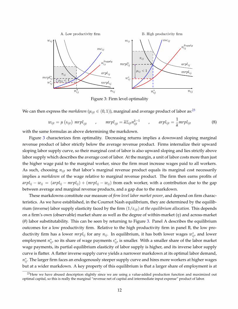
Figure 3: Firm level optimality

We can then express the markdown (µijt ∈ (0, 1)), marginal and average product of labor as:23

wijt = µ(sijt)

mrplijt , mrplijt = αzijtnα−1ijt , arplijt =

1α

mrplijt (8)

with the same formulas as above determining the markdown.Figure 3 characterizes firm optimality. Decreasing returns implies a downward sloping marginal

revenue product of labor strictly below the average revenue product. Firms internalize their upwardsloping labor supply curve, so their marginal cost of labor is also upward sloping and lies strictly abovelabor supply which describes the average cost of labor. At the margin, a unit of labor costs more than justthe higher wage paid to the marginal worker, since the firm must increase wages paid to all workers.As such, choosing nijt so that labor’s marginal revenue product equals its marginal cost necessarilyimplies a markdown of the wage relative to marginal revenue product. The firm then earns profits ofarplij − wij = (arplij − mrplij) + (mrplij − wij) from each worker, with a contribution due to the gapbetween average and marginal revenue products, and a gap due to the markdown.

These markdowns constitute our measure of firm level labor market power, and depend on firm charac-teristics. As we have established, in the Cournot Nash equilibrium, they are determined by the equilib-rium (inverse) labor supply elasticity faced by the firm (1/ε ijt) at the equilibrium allocation. This dependson a firm’s own (observable) market share as well as the degree of within-market (η) and across-market(θ) labor substitutability. This can be seen by returning to Figure 3. Panel A describes the equilibriumoutcomes for a low productivity firm. Relative to the high productivity firm in panel B, the low pro-ductivity firm has a lower mrplij for any nij. In equilibrium, it has both lower wages w∗ij, and loweremployment n∗ij, so its share of wage payments s∗ij, is smaller. With a smaller share of the labor marketwage payments, its partial equilibrium elasticity of labor supply is higher, and its inverse labor supplycurve is flatter. A flatter inverse supply curve yields a narrower markdown at its optimal labor demand,n∗ij. The larger firm faces an endogenously steeper supply curve and hires more workers at higher wagesbut at a wider markdown. A key property of this equilibrium is that a larger share of employment is at

23Here we have abused description slightly since we are using a value-added production function and maximized outoptimal capital, so this is really the marginal “revenue net of capital and intermediate input expense” product of labor.

12

wide markdown firms.

1.5 Characterization - Market equilibrium

Given firm optimality, we establish properties of the market equilibrium and provide an example whichillustrates strategic interactions within the market.

Proposition 1.1. Block recursivity. In each market j ∈ [0, 1], the equilibrium market shares s1jt, . . . , smj jt

satisfy the following mj equations:

sijt =

[µ(sijt)

1−(1−γ)αzijt

] η+1(1−α)(η+1)+αγ

∑mjk=1

[µ(skjt)1−(1−γ)αzkjt

] η+1(1−α)(η+1)+αγ

, µ(sijt) =ε(sijt)

ε(sijt) + 1, ε(sijt) =

[sijtθ

−1 + (1− sijt)η−1]−1

, ∀i = 1, . . . , mj

(9)This system is independent of aggregate variables, and hence the joint distribution µijt, zijt∀ij is determinedunder market equilibrium. Moreover, the payroll share of labor at the market level and market payroll concentrationare given by the following, and hence independent of aggregates:

lsj =∑i∈j wijnij

∑i∈j yij=[∑i∈j

sijls−1ij

]−1= αγ

[∑i∈j

sijµ−1ij

]−1, hhij = ∑

i∈js2

ij.

Proposition (1.1) establishes that the equilibrium of the model is block recursive in that the marketequilibrium can be solved without knowledge of aggregate variables. For the proof see Appendix E.3.This has three significant implications. First, solving the Nash equilibrium in a large J number of marketsis computationally expensive. Proposition (1.1) says that this need only be done once. Second, theaggregate economy can be arbitrarily rich, and feature transition dynamics that do not require re-solvingthe J market equilibria. Third, if it can be shown that an aggregate moment of the economy only dependson the joint distribution of markdowns and productivity, then we know that such moments are robustto alternative assumptions on preferences and capital accumulation. Below we will use only these typesof moments in our calibration, so that our calibration is robust to assumptions on preferences.

The logic underlying the proof of this proposition is that we can consider the equilibrium for the firmas a recursive set of equations that determine the marginal revenue product of labor:

mrplijt = αzijtnα−1ijt , nijt =

(wijt

wjt

)η

njt , wijt = µ(sijt)mrplijt.

This system implies a multiplicative relationship between mrplij and the factors common to all firms inthe market: wjt, njt. Since payroll shares can be expressed in terms of relative wages sijt = (wijt/wjt)

(1+η),the homotheticity of wjt implies that these common factors drop out. For a full proof see Appendix E.

Decreasing returns. The expression for equilibrium payroll shares in Proposition 1.1 is new, and ex-tends such expressions in constant returns oligopoly models to the case of oligopsony, multiple inputs,and decreasing returns. It also provides a novel link between returns to scale and concentration. Con-sider starting with α < 1 and γ = 1, such that labor is the sole input to production. Now consider the

13

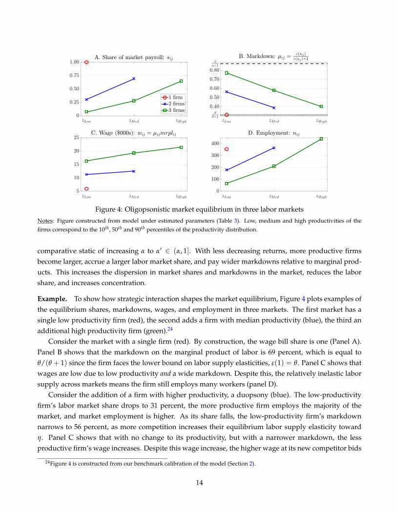
Figure 4: Oligopsonistic market equilibrium in three labor markets

Notes: Figure constructed from model under estimated parameters (Table 3). Low, medium and high productivities of thefirms correspond to the 10th, 50th and 90th percentiles of the productivity distribution.

comparative static of increasing α to α′ ∈ (α, 1]. With less decreasing returns, more productive firmsbecome larger, accrue a larger labor market share, and pay wider markdowns relative to marginal prod-ucts. This increases the dispersion in market shares and markdowns in the market, reduces the laborshare, and increases concentration.

Example. To show how strategic interaction shapes the market equilibrium, Figure 4 plots examples ofthe equilibrium shares, markdowns, wages, and employment in three markets. The first market has asingle low productivity firm (red), the second adds a firm with median productivity (blue), the third anadditional high productivity firm (green).24

Consider the market with a single firm (red). By construction, the wage bill share is one (Panel A).Panel B shows that the markdown on the marginal product of labor is 69 percent, which is equal toθ/(θ + 1) since the firm faces the lower bound on labor supply elasticities, ε(1) = θ. Panel C shows thatwages are low due to low productivity and a wide markdown. Despite this, the relatively inelastic laborsupply across markets means the firm still employs many workers (panel D).

Consider the addition of a firm with higher productivity, a duopsony (blue). The low-productivityfirm’s labor market share drops to 31 percent, the more productive firm employs the majority of themarket, and market employment is higher. As its share falls, the low-productivity firm’s markdownnarrows to 56 percent, as more competition increases their equilibrium labor supply elasticity towardη. Panel C shows that with no change to its productivity, but with a narrower markdown, the lessproductive firm’s wage increases. Despite this wage increase, the higher wage at its new competitor bids

24Figure 4 is constructed from our benchmark calibration of the model (Section 2).

14

away labor, causing the low productivity firm’s employment to fall. Adding another firm (green), themarkdown at the low- and mid-productivity firms decline. The largest firm has the widest markdown(Panel B), but pays more (Panel C) and employs more workers (Panel D).

Figure A2 replicates this exercise with three firms but varying decreasing returns α. Consistent withour above description, higher α generates more concentration and wider markdowns at the leading firm.

Strategic interaction is not an assumption, it’s an outcome of the environment, and leads to a negativecovariance between markdowns and productivity—visible along the green line in Panel B. In equilib-rium, strategic interaction occurs by definition of the Nash equilibrium concept when there is local labormarket power (η > θ) and finitely many firms. In a model of monopsonistic competition, the green linewould be flat, as firms all pay identical markdowns. We now make precise how this negative covariancedistorts the general equilibrium of the economy.

1.6 General equilibrium

Given equilibria in each market of the economy, which determines µijt, zijt∀ij, we state our main propo-sition characterizing the general equilibrium of the economy. For the proof see Appendix E.4.

Proposition 1.2. General equilibrium. The general equilibrium of the model can be characterized in the fol-lowing three steps:

1. Using the market equilibria µijt, zijtmji=1 from all j ∈ [0, 1] markets in the economy, define the following indexes:

Productivity : Z =

[ ˆ 1

0z

1+θ1+θ(1−α)

j dj

] 1+θ(1−α)1+θ

, zj =

[ mj

∑i=1

z1+η

1+η(1−α)

ij

] 1+η(1−α)1+η

Markdown : µ =

[ ˆ 1

0

( zj

Z

) 1+θ1+θ(1−α)

µ1+θ

1+θ(1−α)

j dj

] 1+θ(1−α)1+θ

, µj =

[ mj

∑i=1

(zij

zj

) 1+η1+η(1−α)

µ1+η

1+η(1−α)

ij

] 1+η(1−α)1+η

Misallocation : Ω =

ˆ 1

0

(zij

zj

) 1+θ1+θ(1−α) (µj

µ

) αθ1+θ(1−α)

ωj dj , ωj =

mj

∑i=1

(zij

zj

) 1+η1+η(1−α)

(µij

µj

) ηα1+η(1−α)

2. In steady-state the four aggregate quantities Y , N, C, K and two prices W , R are determined by six equations:

Output and resource constraint: Y = ΩZNα = Ω1−(1−γ)αZ(

K1−γNγ)α

, C = Y − δK

Labor and capital demand: W = γα( µ

Ω

) YN

, R = (1− γ)αYK

Labor and capital supply: W = −UN(C, N)

UC(C, N), 1 = β [R + (1− δ)]

15

where aggregate productivity Z satisfies 25

Z =

[R

(1− γ) α

](1−γ)α[

Z1− (1− γ) α

]1−(1−γ)α

3. Given aggregate quantities and prices, firm level variables can be obtained as follows. First, equating marketlabor demand and market labor supply determines wj and nj. Then, equating firm labor demand and firm laborsupply determines wij and nij:

wj = µjαzjnα−1j︸ ︷︷ ︸

Labor demand

=(nj

N

)1/θ

W︸ ︷︷ ︸Labor supply

, wij = µijαzijnα−1ij︸ ︷︷ ︸

Labor demand

=

(nij

nj

)1/η

wj︸ ︷︷ ︸Labor supply

.

An alternative, intuitive, representation of the aggregate equations can be obtained using the ‘tilde’objects introduced previously, giving four equations determining consumption, output, labor and thewage:

W = − UN(C, N)

UC(C, N)︸ ︷︷ ︸Labor supply

= µαZN α−1

︸ ︷︷ ︸Labor demand

, Y = ΩZN α , C =

[1− δ

R(1− γ) α

]Y

1− α (1− γ).

With respect to an aggregate production function with productivity Z, the markdown µ is a wedgethat pushes the wage below the marginal product of labor, meanwhile for a given productivity Z andemployment N, misallocation Ω represents a direct reduction in output.26 Note that the two termsappear independently.

Benchmark cases. Since welfare is determined by C and N, and Proposition 1.2 allows us to restrictour attention to understanding markdowns µ and misallocation Ω. Three benchmarks are useful:

- Case I - Efficient allocation. The efficient allocation coincides with an economy in which firm-by-firm wages and marginal revenue products of labor are aligned, that is µij = 1 for all firms. In thiscase µ = 1, and Ω = 1.

- Case II - Monopsony limits. A monopsonistically competitive economy attains under either of twolimits: (1) mj → ∞ or (2) θ → η. Henceforth we simply refer to these conditions as the “monopsonylimits”. Under either limit, firms are infinitesimal in the markets in which they set wages. In thefirst limit, they face a highly competitive local market. In the second limit, they face a national

25Note that we could directly compute productivity Z using only primitives: zj :=[

∑i∈j z1+η

1−(1−γ)α+η(1−α)

ij] 1−(1−γ)α+η(1−α)

1+η and

Z :=[ ´

z1+θ

1−(1−γ)α+θ(1−α)

j dj] 1−(1−γ)α+θ(1−α)

1+θ . Using these as primitives leads to long exponents on the µj, µ, ωj, and Ω terms, hencewe state the proposition in terms of effective productivities after the firms’ optimal capital choice.

26Another way to see this is to define the following production function for competitive intermediate goods producers:Y = ZN α. The labor demanded by these producers is given by W = µαZN α−1. A final goods producer with productivityΩ < 1 then converts intermediates into final goods.

16

market. Markdowns µij are identical across firms and equal to η/(η + 1), as market shares sij → 0.In this case µ = E

[µij], and Ω = 1.

- Case III - Full model. In our full model, the negative correlation of productivity and markdownswithin markets (recall Figure 4), leads to (i) Ω < 1, which reduces output, and (ii) a higher produc-tivity weight on wide markdown firms, lowering µ < E

[µij].

These special cases reveal that the oligopsonistic economy we have contributed distorts welfare relativeto a monopsonistically competitive economy precisely through misallocation Ω. In a monoposonisticallycompetitive economy, the labor supply elasticity to the firm η could be calibrated to generate the sameµ, yet it would still feature Ω = 1. That Ω < 1 is an outcome of the counterpart of both limits (i) labormarkets are concentrated, and (ii) market power via θ < η.

This characterization of the model situates the remainder of our paper. First, we provide new empir-ical facts that allow us—along with the structure of the model—to credibly estimate θ and η. Second, weshow that θ < η is necessary for the model to qualitatively and quantitatively match the sign and mag-nitude of non-targeted empirical evidence on pass-through and strategic wage-setting of firms. Third,we show that the implied misallocation Ω due to θ < η accounts for around half of the welfare lossesdue to labor market power, and that this is robust to specifications of aggregate preferences.

1.7 Measurement

The general equilibrium of the model can be used to show that the following two measures of the labormarket are independent of the specification of the macroeconomy. We use these results in our calibrationexercise in the next section.

Proposition 1.3. Labor share and concentration.

- The aggregate labor share depends only on the distribution of markdowns and productivity

LSt :=

´ 10 ∑

mji=1 wijnij dj´ 1

0 ∑mji=1 yij dj

=W N

Y= γα

( µ

Ω

)- The across market payroll-weighted average of payroll concentration, which we simply refer to as the

wage-bill Herfindahl, is defined

HHIwnt =

ˆ 1

0sjt hhiwn

jt dj , hhiwnjt =

mj

∑i=1

s2ijt , sjt =

∑i∈j wijtnijt´ 10 ∑i∈j wijtnijt dj

,

- The two are linked by the following equation, and hence HHIwnt depends only on the distribution of mark-

downs and productivity

LSt =

ˆ 1

0sjtlsjt dj = αγ︸︷︷︸

Competitive LS

[HHIwn

t

(θ

θ + 1

)−1

+(

1− HHIwnt

)( η

η + 1

)−1]−1

︸ ︷︷ ︸Labor market power adjustment

(10)

17

For a full derivation of these results see Appendix E.5. Consider again the three benchmark cases.In an efficient economy, labor share is equal to the output elasticity γα and concentration plays no role.Under monopsony due to mj → ∞, the Herfindahl in each market is zero, all firms have a markdownµij = η/(η + 1), but with Ω = 1 the labor share is γαµ. Under monopsony due to θ → η, the Herfindahlin each market is positive but does not appear in the labor share. There is a meaningful relationshipbetween concentration and the labor share only under oligopsony with θ < η.

In such an economy, higher concentration reduces the labor share. Intuitively, this expression arisesin two steps. At the market level, the HHI measures the payroll share of high payroll share firms, whichin our model have wide markdowns and so low labor shares. Aggregating across firms within eachmarket delivers (10) in the cross-section of markets. At the aggregate level, the aggregate labor share isthe payroll weighted average of market labor shares, leading to (10).

Note that HHIwnjt and LSt are not sufficient statistics for welfare, even when combined with all other

parameters of the model. Combined they reveal the ratio (µ/Ω), but cannot be used to disentangle thetwo. Proposition 1.2 established that both are required independently in order to compute aggregatequantities and hence welfare. Intuitively, the labor share and Herfindahl capture the wedge in the labordemand condition, but still do not capture the output wedge Ω.

Nonetheless, this model-implied measure of labor market concentration differs from all existing stud-ies. For example, recent work by Benmelech, Bergman, and Kim (2020) and Rinz (2018) use employ-ment Herfindahls and various weighting schemes. Independent of our model framework, employmentHerfindahls understate concentration since they ignore the positive relationship between wages andemployment, which is a robust feature of the data (Brown and Medoff, 1989; Lallemand, Plasman, andRycx, 2007; Bloom, Guvenen, Smith, Song, and von Wachter, 2018).27 We return to study the model’simplication for the labor share through the lens of changing HHIwn

t and equation (10) in Section 5.

2 Estimation

Our key parameters to estimate are the degree of across- (θ) and within- (η) market labor substitutabil-ity. In this section, we describe our novel approach which integrates (i) new empirical estimates froma quasi-natural experiment and (ii) new moments from the cross-section of markets given in (for addi-tional moments see Table D1), into (iii) a simulated method of moments routine in which all unknownparameters are estimated jointly.

2.1 Approach - Structural vs. reduced-form labor supply elasticities

Structural elasticities. We motivate our approach from the following observation. If a researcher couldestimate the structural elasticities of labor supply that firms perceive at the Nash equilibrium level of em-ployment, then they could combine data on payroll shares and one of the key model equations to esti-

27For a complete proof of this claim see Appendix E. The unconditional firm-level correlation of log employment and logwages is 0.30 in our 2014 tradeable industries LBD sample.

18

mate (θ, η):

ε(

swnij , θ, η

):=

[∂ log wijt

∂ log nij

(swn

ij

) ∣∣∣∣n∗−ij

]−1

=

[1η

(1− swn

ij

)+

1θ

swnij

]−1

. (11)

In particular, a decreasing relationship between ε ij and swnij would identify η > θ.

Reduced form elasticities. When firms behave strategically the structural elasticity cannot be mea-sured using wage and employment responses to well identified firm-level shocks. As is clear from thenotation above, the structural elasticity is a strictly partial equilibrium concept and answers the counter-factual: How much will firm ij have to increase wij in order to expand nij by one percent, holding its competitors’employment fixed? Given a shock to any firm in the market, an employment change at firm i will leadcompetitors to best-respond, which will cause i to best respond and so on. What an empiricist wouldmeasure in the data following a shock is therefore a reduced-form elasticity ε(sijt, θ, η, . . . ), which includeall other firms’ employment and wage changes across market equilibria.28

Our insight is that, despite this, the reduced-form elasticities that we may aspire to measure, oncefiltered through our structural model, are still informative of (θ, η). To a first order approximation, thereduced-form elasticity of labor supply a researcher would measure for firm ij following a shock to it ora competitor is (for derivation see Appendix E.7):

ε(

swnijt , θ, η, . . .

):=

d log nijt

d log wijt=

⟨1

1 + ε(

swnijt , θ, η

) (η−θθη

) ∑k 6=i swn

kjtd log nkjtd log nijt

⟩× ε(

swnijt , θ, η

). (12)

A distinct property of (12) is that reduced form and structural elasticities coincide exactly under themonopsony limits. As θ → η, the term 〈·〉 goes to one. As sijt → 0, then the perturbed firm is infinites-imal so competitors do not respond and the equilibrium interaction term · goes to zero. Outside themonopsony limits, strategic interaction implies that reduced-form estimates of labor supply elasticitiescannot be used to directly infer welfare-relevant labor supply elasticities.

Bias. The relationship between structural and reduced-form elasticities varies predictably dependingon whether the underlying shock is idiosyncratic or common across multiple – but not all – firms in amarket. A common shock to all firms drops out from the market equilibrium condition in Proposition1.1 and could only be used to estimate the market level labor supply elasticity.

First, consider a positive idiosyncratic productivity shock to firm i in market j such that the firmexpands employment. As the firm expands employment, its competitors respond. Since competitionis Cournot, employment levels across firms are strategic substitutes so competitors reduce employment(d log nkjt < 0), implying that the equilibrium interaction term is negative, · < 0, and the reduced-form elasticity exceeds the structural elasticity: ε(swn

ijt , θ, η) > ε(swnijt , θ, η). Figure 5A illustrates this case.

The contraction in employment at competitors expands labor supply to the firm. An observer drawingconclusions about labor market power from the high reduced-form labor supply elasticity would con-

28We borrow the notation of ε for reduced-form elasticities and ε for structural elasticities from the estimation of structuralmacroeconomic models. In this literature reduced-form shocks which are empirical objects estimated out of VARs are oftendenoted ε, and structural shocks that are backed out of an estimated structural model are denoted ε.

19

clude labor markets are more competitive than they are. Later in this section, we show that this biasis quantitatively significant: inferred structural and reduced-form elasticities differ by up to 50 percent,even for perfectly idiosyncratic shocks.

For non-idiosyncratic shocks that are common across a subset of firms, we reach the opposite conclu-sion. Consider a tax cut that affects firm i in market j as well as the other large firms in market j. Call theseaffected firms C-Corps. Suppose the tax cut induces firm i and all affected C-Corps to expand employ-ment, i.e. d log nijt > 0 and d log nkjt > 0 for all firms-kj that are C-Corps. If non-C-Corp firms have smallshares (skjt ≈ 0), their strategic response is irrelevant. The equilibrium interaction term will be positive

· > 0, and the reduced-form elasticity understates the structural elasticity: ε(

swnijt , θ, η

)< ε(

swnijt , θ, η

).

Figure 5B illustrates this case. The expansion in employment at competing C-Corps contracts labor sup-ply to the firm. An observer drawing conclusions about labor market power from the low reduced-formlabor supply elasticity would conclude that labor markets are less competitive than they are.

Indirect inference. The above demonstrates that reduced-form elasticities are informative of structuralelasticities which are in turn informative about welfare relevant parameters, and that the equilibriumstructure of the model is necessary to complete this mapping. Our approach recognizes this. We firstuse a quasi-natural policy experiment to estimate the relationship between payroll shares and averagereduced-form labor supply elasticities in the data: εData(s). We then replicate the same policy experimentin our model which yields

εModel(

s, θ, η)

:= E[εModel

(s, θ, η, . . .

)],

where the expectation is being taken with respect to the distribution of all relevant labor market variablesand shocks. We then choose (θ, η)—along with other parameters—to replicate the empirical relationshipbetween average reduced-form elasticities and payroll shares.

2.2 Estimating reduced-form labor supply elasticities in the data: εData(s)

We estimate size-dependent reduced-form labor supply elasticities using state corporate tax changesin conjunction with the Census Longitudinal Business Database (LBD). The LBD provides high qualitymeasures of employment, location, and industry with nearly universal coverage of the non-farm busi-ness sector. Data are carefully linked over time at the establishment and firm level. In order to proceed,we first define markets and firms. We then describe our regression approach.

Market. In our model, a labor market has two features: (i) a worker drawn at random from the economywill have a greater attachment to one labor market than others on the basis of idiosyncratic preferences,but will nonetheless be able to move across markets, and (ii) firms within a market compete strategically.

With these features in mind and given what we can observe in the LBD, we define a local labor marketas a 3-digit NAICS (NAICS3) industry within a Commuting Zone (CZ).29 Examples of adjacent 3-digit

29Using BLS Occupational Employment Statistics microdata, Handwerker and Dey (2018) show that when it comes to con-centration there is little practical difference in defining a market at the occupation-city level rather than the industry-city levelas these two measures are highly correlated. In particular, the across-city correlation of Herfindahl-Hirschman Indices at theCBSA-occupation and CBSA-industry level is 0.97.

20

NAICS codes are subsectors 323-325: ‘Printing and Related Support Activities’, ‘Petroleum and Coal ProductsManufacturing’ and ‘Chemical Manufacturing’ which we regard as suitably different. Examples of adja-cent commuting zones include the collection of counties surrounding downtown Minneapolis and thosesurrounding Duluth.30

Firm. We define a firm in a local labor market as the collection of establishments operated by that firm.We aggregate employment and annual payroll of all establishments owned by the same firm within thesame NAICS3-CZ market.31 For each resulting firm-market-year observation, we observe employment,payroll, and herein define the wage as payroll per worker.

Regression framework. To estimate the relationship εData(s) in the data we use within-firm-market,across-time changes in wages and employment following state corporate tax changes.

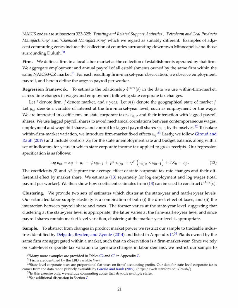
Let i denote firm, j denote market, and t year. Let s(j) denote the geographical state of market j.Let yijt denote a variable of interest at the firm-market-year level, such as employment or the wage.We are interested in coefficients on state corporate taxes τs(j)t and their interaction with lagged payrollshares. We use lagged payroll shares to avoid mechanical correlations between contemporaneous wages,employment and wage-bill shares, and control for lagged payroll shares sijt−1 by themselves.32 To isolatewithin-firm-market variation, we introduce firm-market fixed effects αij.33 Lastly, we follow Giroud andRauh (2019) and include controls Xit for the state unemployment rate and budget balance, along with aset of indicators for years in which state corporate income tax applied to gross receipts. Our regressionspecification is as follows:

log yijt = αij + µt + ψ sijt−1 + βy τs(j)t + γy(

τs(j)t × sijt−1

)+ ΓXit + νijt. (13)

The coefficients βy and γy capture the average effect of state corporate tax rate changes and their dif-ferential effect by market share. We estimate (13) separately for log employment and log wages (totalpayroll per worker). We then show how coefficient estimates from (13) can be used to construct εData(s).

Clustering. We provide two sets of estimates which cluster at the state-year and market-year levels.Our estimated labor supply elasticity is a combination of both (i) the direct effect of taxes, and (ii) theinteraction between payroll share and taxes. The former varies at the state-year level suggesting thatclustering at the state-year level is appropriate; the latter varies at the firm-market-year level and sincepayroll shares contain market level variation, clustering at the market-year level is appropriate.

Sample. To abstract from changes in product market power we restrict our sample to tradeable indus-tries identified by Delgado, Bryden, and Zyontz (2014) and listed in Appendix C.34 Plants owned by thesame firm are aggregated within a market, such that an observation is a firm-market-year. Since we relyon state-level corporate tax variation to generate changes in labor demand, we restrict our sample to

30Many more examples are provided in Tables C2 and C3 in Appendix C.31Firms are identified by the LBD variable firmid.32State-level corporate taxes are proportional flat-taxes on firms’ accounting profits. Our data for state-level corporate taxes

comes from the data made publicly available by Giroud and Rauh (2019): (https://web.stanford.edu/ rauh/).33In this exercise only, we exclude commuting zones that straddle multiple states.34See additional discussion in Section C

21

C-Corporation firms (C-Corps) in the LBD from 1977 to 2011. Table C1 includes summary statistics ofour 2.8 million observations at the firm-market-year level.

Estimates. Table 1 presents empirical estimates of (13). We start with (log) employment in year t as adependent variable. Column (1) presents the full set of interaction terms between payroll shares andcorporate taxes. Since τs(j)t is in units of percents, the coefficient on τs(j)t is an elasticity: a one percentincrease in corporate taxes results in a 0.309 percent reduction in employment at firms that are atomisticwithin the market (sijt−1 = 0). The interaction term is positive and significant. When combined withthe negative direct effect, the interaction indicates a dampened response at larger firms. Compare themean effect of a 1 ppt increase in τs(j)t on a firm with a mean payroll share (0.03) to a firm with a onestandard deviation higher share (0.10). Employment declines by −0.26 percent at the small firm and−0.15 percent at the large firm. Consistent with Giroud and Rauh (2019), increases in corporate tax ratesreduce employment. Our empirical finding is that this reduction is around 40 percent weaker at largerfirms.

Column (2) illustrates estimates of (13) when the dependent variable is the wage. Qualitatively thesigns echo the employment response: on average wages fall, and this decline is smaller at larger firms.Columns (3) and (4) provide estimates of (13) using year t + 1 employment and wages as dependentvariables. These specifications are designed to accommodate adjustment frictions in prices and quan-tities. We again find a negative effect of corporate taxes on employment and wages, with diminishedeffects at larger firms.

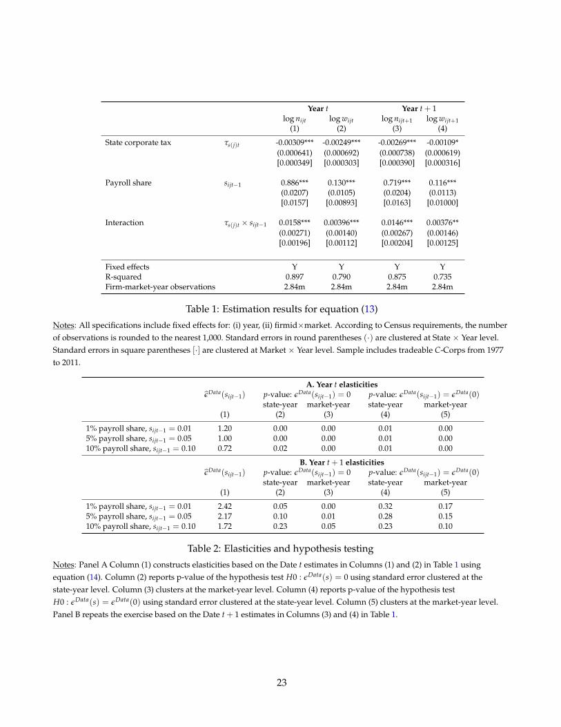
Share-dependent reduced-form labor supply elasticities. Table 2 combines the wage and employmentresponses to compute the relationship between the average reduced-form labor supply elasticity andpayroll shares, which informs both θ and η. Differentiating (13) with respect to τs(j)t delivers share-dependent reduced-form wage and employment elasticities:

d log nijt

dτs(j)t= βn + γnsijt−1 ,

d log wijt

dτs(j)t= βw + γwsijt−1 , εData(sijt−1) =

d log nijt

d log wijt

=βn + γnsijt−1

βw + γwsijt−1(14)

When we turn to indirect inference, we run the same regressions on model simulated data to computeεModel(s) in the same way.

Column (1) of Table 2A reports reduced-form labor supply elasticity estimates εData(sijt−1) based onthe Table 1 Year t estimates for sijt−1 ∈ 0.01, 0.05, 0.10. At a wage bill share of 1 percent, the yeart reduced-form labor supply elasticity is 1.20, and declines to 0.72 at a wage bill share of 10 percent.Columns (2) and (3) show that the elasticity is statistically significant at the 5 percent level under eitherassumption for clustering.

In Columns (4) and (5) of Table 2A, we test whether the estimated date t labor supply elasticities oflarger firms are statistically different from atomistic firms. Formally, we test H0 : εData(sijt−1) = εData(0)for sijt−1 ∈ 0.01, 0.05, 0.10. In each case the year t reduced-form labor supply elasticities in column (1)is significantly different from that of an atomistic firm at the 1 percent level.

Table 2B repeats the same exercise for year t + 1 employment and wage responses from columns (3)

22

Year t Year t + 1log nijt log wijt log nijt+1 log wijt+1

(1) (2) (3) (4)

State corporate tax τs(j)t -0.00309*** -0.00249*** -0.00269*** -0.00109*(0.000641) (0.000692) (0.000738) (0.000619)[0.000349] [0.000303] [0.000390] [0.000316]

Payroll share sijt−1 0.886*** 0.130*** 0.719*** 0.116***(0.0207) (0.0105) (0.0204) (0.0113)[0.0157] [0.00893] [0.0163] [0.01000]

Interaction τs(j)t × sijt−1 0.0158*** 0.00396*** 0.0146*** 0.00376**(0.00271) (0.00140) (0.00267) (0.00146)[0.00196] [0.00112] [0.00204] [0.00125]

Fixed effects Y Y Y YR-squared 0.897 0.790 0.875 0.735Firm-market-year observations 2.84m 2.84m 2.84m 2.84m

Table 1: Estimation results for equation (13)

Notes: All specifications include fixed effects for: (i) year, (ii) firmid×market. According to Census requirements, the numberof observations is rounded to the nearest 1,000. Standard errors in round parentheses (·) are clustered at State × Year level.Standard errors in square parentheses [·] are clustered at Market × Year level. Sample includes tradeable C-Corps from 1977to 2011.

A. Year t elasticitiesεData(sijt−1) p-value: εData(sijt−1) = 0 p-value: εData(sijt−1) = εData(0)

state-year market-year state-year market-year(1) (2) (3) (4) (5)

1% payroll share, sijt−1 = 0.01 1.20 0.00 0.00 0.01 0.005% payroll share, sijt−1 = 0.05 1.00 0.00 0.00 0.01 0.0010% payroll share, sijt−1 = 0.10 0.72 0.02 0.00 0.01 0.00

B. Year t + 1 elasticitiesεData(sijt−1) p-value: εData(sijt−1) = 0 p-value: εData(sijt−1) = εData(0)

state-year market-year state-year market-year(1) (2) (3) (4) (5)

1% payroll share, sijt−1 = 0.01 2.42 0.05 0.00 0.32 0.175% payroll share, sijt−1 = 0.05 2.17 0.10 0.01 0.28 0.1510% payroll share, sijt−1 = 0.10 1.72 0.23 0.05 0.23 0.10

Table 2: Elasticities and hypothesis testing

Notes: Panel A Column (1) constructs elasticities based on the Date t estimates in Columns (1) and (2) in Table 1 usingequation (14). Column (2) reports p-value of the hypothesis test H0 : εData(s) = 0 using standard error clustered at thestate-year level. Column (3) clusters at the market-year level. Column (4) reports p-value of the hypothesis testH0 : εData(s) = εData(0) using standard error clustered at the state-year level. Column (5) clusters at the market-year level.Panel B repeats the exercise based on the Date t + 1 estimates in Columns (3) and (4) in Table 1.

23

and (4) of Table 1. At year t + 1 the implied reduced-form labor supply elasticities are larger, potentiallydue to slow employment adjustment. However, the estimates are noisier. Based on year t + 1 estimateswe cannot statistically distinguish εData(sijt−1) from εData(0) for sijt−1 ∈ 0.01, 0.05, 0.10. At a wage-billshare of 10 percent, we come closest to distinguishing the year t + 1 reduced-form labor supply elasticityfrom that of an atomistic firm at the 10 percent level.

In summary, our more precise year t estimates of the size-dependent wage and employment responseindicate (i) less responsiveness of larger firms, and (ii) significantly lower reduced-form labor supplyelasticities of larger firms. Our year t + 1 estimates imply greater labor supply elasticities across all firmsizes, consistent with frictional adjustment. In both cases we find that larger firms have lower laborsupply elasticities; however, we lack the power to statistically distinguish the labor supply elasticity oflarge firms from small firms in the year t + 1 case.

Additional results. Appendix G.3 provides additional results. First, model estimation simply requiresconsistent auxiliary moments that can be simulated. The threat to consistency when we estimate equation(13) is that other forces move employment and wages at the state-year level (e.g. taxes are cut when un-employed is low). Table G3 shows that our main interaction between corporate taxes and the wage-billshare is robust to the inclusion of state-year fixed effects, thus removing all common state-year variation.Second, we directly compute the ratio of wage changes to employment changes at the firm-level andstudy their relationship with firms’ wage-bill share. Following corporate tax cuts, we estimate statisti-cally significantly different labor supply elasticities at large relative to atomistic firms. Third, using the2012 Census of Manufacturers, we show that variation in non-wage compensation is unable to explainthe large movements in markdowns implied by our baseline labor supply elasticity estimates. Finally,we show that systematic variation in capital intensity by market share cannot explain our results: withinmarkets, capital intensity and payroll shares are only weakly correlated.

2.3 Simulating reduced-form labor supply elasticities in the model: εModel(s, θ, η)

To construct εModel(s, θ, η), we add corporate taxes to the environment and show how they shift marginalrevenue products of labor. We make several modifications to our theory. Corporate taxes are a taxon profits, net of interest payments on debt. Firms finance λK ∈ [0, 1] of their capital using debt andmaximize post-tax profits:

πijt =(

1− τC

)zijt

(k1−γ

ijt nγijt

)α−(

1− τCλK

)Rkijt −

(1− τC

)w(nijt)nijt,

A random fraction ωC ∈ [0, 1] of firms in each market are C-corps and subject to τC; all other firms faceτC = 0. In the data, C-corps are larger on average. To capture this we assume a productivity premium∆C > 1:

log(zijt) ∼

N(

1, σ2z

)if i is not a C-corp (i.e. with probability 1−ωC)

N(

∆C, σ2z

)if i is a C-corp (i.e. with probability ωC)

24

For C-corps, the corporate tax distorts their capital decision, which reduces the marginal product oflabor. Under the firm’s optimal capital demand, effective productivity zijt is decreasing in τC if λK > 0:

πijt

1− τC= max

nijtzijtnα

ijt−w(nijt)nijt , zijt =

[1− τC

1− τCλK

] α(1−γ)1−α(1−γ)

×⟨[1− α (1− γ)]

(α (1− γ)

Rt

) α(1−γ)1−α(1−γ)

z1

1−α(1−γ)

ijt

⟩,

see Appendix E.9. With these modifications to the theory, we can simulate an increase in corporate taxesand estimate reduced-form elasticities consistent with our approach to the data to obtain εModel(s, θ, η).

2.4 Indirect inference

We estimate the model using 2014 Census data and proceed in two steps. First, to match the reduced-form elasticities measured in a sample of tradeable firms, we estimate a tradeable-only version of oureconomy. This includes the corporate tax experiment and yields estimates of the key preference pa-rameters η and θ. Second, holding η and θ fixed, we drop the corporate tax experiment and estimatethe remaining parameters to match economy-wide moments. The tradeable sector is more concentratedthan the economy on the whole, so the second step is necessary for measuring labor market power inthe US economy. We add to the model a parameter that shifts firm productivity Z, and a preferenceparameter that shifts labor supply ϕ.

Common external parameters. On an annual basis, the discount rate is 4 percent (β = 0.9615), andthe depreciation rate is 10 percent (δ = 0.10). Throughout we simulate 5, 000 markets and verify thatour results are not sensitive to this choice. The moments used in our estimation are robust to alternativespecifications of aggregate preferences U(C, N), so we defer specifying U until we evaluate welfare.

Tradeable only - External parameters. To capture the distribution of tradeable firms across markets,mj ∼ G(mj) we combine a Pareto distribution with a discrete mass at mj = 1 to capture single firmmarkets. The mass of tradeable markets with a single firm is 16 percent (Table F1). We fit the remainingPareto parameters to match the first three moments of the distribution of firms across markets. AppendixTable F1 provides moments and parameter estimates.

The fraction of capital financed by debt is chosen to match the debt to capital ratio among tradeablefirms. For this we use tradeable firms in Compustat and obtain λK = 0.213. A fraction ωC = 0.42 offirms are C-corps based on the 2014 County Business Patterns data for tradeable sectors (CBP).

Given parameters we simulate a three-period panel from the model. The first two periods are givenby the model’s steady state with τC set to the mean state corporate tax rate of 6.9 percent (the averageover the sample period 1977 to 2011). In the third period, we increase taxes by ∆τ = one percentagepoint, which is approximately one standard deviation of the distribution of state corporate tax changesobserved in our sample period.35 Treating model output as panel data, we estimate (13) with firm fixedeffects and lagged payroll shares (hence the requirement for three periods). We replicate our treatmentof the data, and transform point estimates into average reduced-form elasticities by payroll share usingequation (14). Appendix F includes additional details on simulating the tax experiment.

35We use data made publicly available by Giroud and Rauh (2019)

25

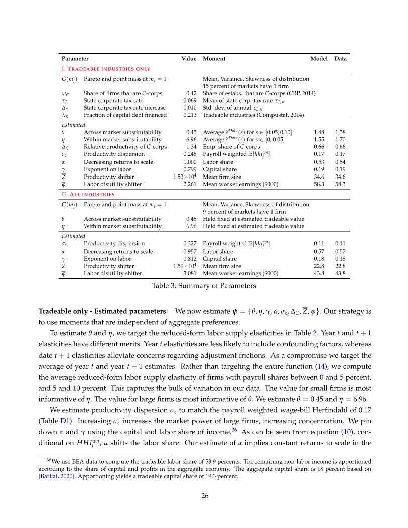
Parameter Value Moment Model Data

I. TRADEABLE INDUSTRIES ONLY

G(mj) Pareto and point mass at mj = 1 Mean, Variance, Skewness of distribution15 percent of markets have 1 firm

ωC Share of firms that are C-corps 0.42 Share of estabs. that are C-corps (CBP, 2014)τC State corporate tax rate 0.069 Mean of state corp. tax rate τC,st∆τ State corporate tax rate increase 0.010 Std. dev. of annual τC,stλK Fraction of capital debt financed 0.213 Tradeable industries (Compustat, 2014)

Estimatedθ Across market substitutability 0.45 Average εData(s) for s ∈ [0.05, 0.10] 1.48 1.38η Within market substitutability 6.96 Average εData(s) for s ∈ [0, 0.05] 1.55 1.70∆C Relative productivity of C-corps 1.34 Emp. share of C-corps 0.66 0.66σz Productivity dispersion 0.248 Payroll weighted E[hhiwn

j ] 0.17 0.17α Decreasing returns to scale 1.000 Labor share 0.53 0.54γ Exponent on labor 0.799 Capital share 0.19 0.19Z Productivity shifter 1.53×104 Mean firm size 34.6 34.6ϕ Labor disutility shifter 2.261 Mean worker earnings ($000) 58.3 58.3

II. ALL INDUSTRIES

G(mj) Pareto and point mass at mj = 1 Mean, Variance, Skewness of distribution9 percent of markets have 1 firm

θ Across market substitutability 0.45 Held fixed at estimated tradeable valueη Within market substitutability 6.96 Held fixed at estimated tradeable value

Estimatedσz Productivity dispersion 0.327 Payroll weighted E[hhiwn

j ] 0.11 0.11α Decreasing returns to scale 0.957 Labor share 0.57 0.57γ Exponent on labor 0.812 Capital share 0.18 0.18Z Productivity shifter 1.59×104 Mean firm size 22.8 22.8ϕ Labor disutility shifter 3.081 Mean worker earnings ($000) 43.8 43.8

Table 3: Summary of Parameters

Tradeable only - Estimated parameters. We now estimate ψ = θ, η, γ, α, σz, ∆C, Z, ϕ. Our strategy isto use moments that are independent of aggregate preferences.

To estimate θ and η, we target the reduced-form labor supply elasticities in Table 2. Year t and t + 1elasticities have different merits. Year t elasticities are less likely to include confounding factors, whereasdate t + 1 elasticities alleviate concerns regarding adjustment frictions. As a compromise we target theaverage of year t and year t + 1 estimates. Rather than targeting the entire function (14), we computethe average reduced-form labor supply elasticity of firms with payroll shares between 0 and 5 percent,and 5 and 10 percent. This captures the bulk of variation in our data. The value for small firms is mostinformative of η. The value for large firms is most informative of θ. We estimate θ = 0.45 and η = 6.96.

We estimate productivity dispersion σz to match the payroll weighted wage-bill Herfindahl of 0.17(Table D1). Increasing σz increases the market power of large firms, increasing concentration. We pindown α and γ using the capital and labor share of income.36 As can be seen from equation (10), con-ditional on HHIwn

t , α shifts the labor share. Our estimate of α implies constant returns to scale in the

36We use BEA data to compute the tradeable labor share of 53.9 percents. The remaining non-labor income is apportionedaccording to the share of capital and profits in the aggregate economy. The aggregate capital share is 18 percent based on(Barkai, 2020). Apportioning yields a tradeable capital share of 19.3 percent.

26

tradeable sector. Parameter γ matches the aggregate capital share. Table 3 summarizes all parametersand the model’s fit to the target moments. In Appendix E.6 we provide a closed form solution of themodel and prove that in any equilibrium (Z, ϕ) normalize units of wages and labor, so are chosen tomatch average firm size (34.6) and payroll per worker ($58, 300) (Table D1). Finally, ∆C matches the 66percent employment share of C-corps (CBP).

Economy-wide calibration. Holding our estimates of preference parameters η and θ fixed, we recali-brate our model to match economy-wide moments. We update the distribution of firms across marketsG(mj), which almost halves the number of markets with one firm to 9 percent. We remove C-corps,setting ωC = 0 and estimate ψ = γ, α, σz, Z, ϕ to match, the (i) labor share, (ii) capital share, (iii)payroll-weighted wage-bill Herfindahl, (iv) average firm size, and (v) average payroll per worker. No-tably, in the overall economy, concentration is lower, the labor share is higher and wages and averagefirm size are smaller. With less concentration market power is lower, reducing profits, hence a lowervalue of α is required to increase profits. The model matches the data exactly and yields decreasingreturns to scale, α = 0.957.

2.5 Discussion of estimated θ and η

Figure 5C plots εData(sijt−1) over sijt−1 ∈ [0, 0.10]. The model generates a downward sloping reduced-form labor supply elasticity similar to the data. Notably, the reduced-form estimates for atomistic firmsare roughly four times smaller than the structural estimates. Thus, a naive estimation would concludethat the labor market is less competitive than it actually is, and infer markdowns at atomistic firms of0.65. Our structural estimates of the labor supply elasticity at atomistic firms imply a markdown of only0.87 percent, roughly 3 times narrower. The upward bias in market power implied from naive use ofreduced-form estimates is less pronounced among larger firms. These predictions are in line with ourtheory of non-idiosyncratic shocks in Panel B.

Entry and Exit. One concern may be that following a tax increase some firms may exit, and this mayaffect our estimates of θ and η. To address this we conduct two exercises. First, in Appendix G weestimate linear probability models of firm-market exit in year t + 1 as a function of corporate taxes inyear t. We find economically insignificant results. Giroud and Rauh (2019) find that firms adjust theirtotal number of plants in the state. Our results imply that they do not appear to be exiting commuting-zone markets entirely in response to corporate tax changes. Second, despite these insignificant empiricalresults, we estimate the model under the extreme counterfactual assumption that the smallest 5 percentof C-corps in each market exit after the tax increase. Our estimates of θ and η are unchanged. Details ofthis exercise are in Appendix G.2.

Idiosyncratic shocks and bias. So far, our analysis has focused on bias between reduced-form andstructural elasticities when the observed shock is non-idiosyncratic, illustrated in Figure 5B. In this sec-tion, we quantify the bias under idiosyncratic shocks, illustrated in Figure 5A. Many existing papers relyon estimation strategies that assume atomistic firms and infer monopsony from firm-level responses to

27

Figure 5: Reduced form and structural labor supply elastictiesNotes: Panel A demonstrates the relationship between reduced-form and structural labor supply elasticities for an idiosyn-cratic shock. Panel B demonstrates the relationship between reduced-form and structural labor supply elasticities for a non-idiosyncratic shock that affects a proper subset of firms. Panel C compares reduced-form and structural labor supply elasticitiesby firm payroll share in response to a corporate tax shock of 1 percentage point. ‘Data t + 1 - Reduced form’ plots the date t + 1empirical labor supply elasticity estimates in Table 2. ‘Data t - Reduced form’ plots the date t empirical labor supply elasticityestimates in Table 2. ‘Data mid - Reduced form’ is an equally weighted average of the date t + 1 and date t empirical laborsupply elasticity estimates in Table 2. ‘Model - Reduced form t’ plots reduced-form labor supply elasticity estimates, estimatedon simulated model data as described in Appendix F.2. ’Model - Structural’ plots ε(·) from equation (11).

idiosyncratic shocks (e.g., see the articles surveyed in Card, Cardoso, Heining, and Kline (2018)). Weshow that using data on employment and wage changes in response to identified firm-level shocks toinfer key structural parameters may generate sizeable bias.

Consider a truly idiosyncratic shock to a single randomly selected firm in our economy. Drawing thetreated firm at random, compute the reduced form elasticity εij and compare it to the structural elastic-ity ε ij. We repeat this 5,000 times for small (one percent), medium (10 percent) and large (50 percent)productivity shocks. We plot the results in Figure 6. This Monte Carlo exercise reveals a significant dif-ference in reduced-form and structural labor supply elasticities for firms with market shares not equal to0 or 1, even when the identifying variation is perfectly idiosyncratic. The bias between reduced-form andstructural elasticities is 18 percent for firms with market shares between 0 and 10% that receive smallshocks (1% productivity increase). This bias increases to over 23% for medium and large shocks. Ac-counting for the Nash equilibrium of the local labor market is quantitatively important for recoveringwelfare relevant parameters.

This exercise implies that even if a researcher aims to use perfect idiosyncratic variation in produc-tivity to infer structural elasticities and do welfare analysis, they would have to deflate their reduced-formelasticity estimates substantially in order to recover the true structural elasticities. Inferring structural elas-ticities that are too large one would infer narrower markdowns which would bias downward the welfarelosses due to labor market power. The details of our Monte Carlo exercise are included in Appendix F.3.

Figure 6 shows that two important caveats apply, both summarized in equation (12). If the firm hasa share of one, then reduced-form and structural elasticity estimates coincide and reveal θ. If the firmhas an infinitesimal share, then reduced-form and structural elasticity estimates coincide and reveal η.Finally, a market level shock will directly reveal θ, so long as the market itself is not large. If the market isvery large then a market level shock will also effect the macroeconomic equilibrium of the labor market,

28

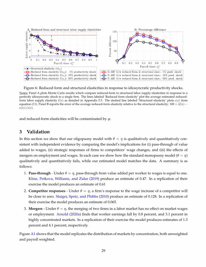
Figure 6: Reduced form and structural elasticities in response to idiosyncratic productivity shocks.Notes: Panel A plots Monte Carlo results which compare reduced-form to structural labor supply elasticities in response to aperfectly idiosyncratic shock to a single firm. The lines labeled ‘Reduced form elasticity’ plot the average estimated reduced-form labor supply elasticity ε(s) as detailed in Appendix F.3. The dashed line labeled ‘Structural elasticity’ plots ε(s) fromequation (11). Panel B reports the error of the average reduced-form elasticity relative to the structural elasticity: 100× (ε(s)−ε(s))/ε(s).

and reduced-form elasticities will be contaminated by ϕ.

3 ValidationIn this section we show that our oligopsony model with θ < η is qualitatively and quantitatively con-sistent with independent evidence by comparing the model’s implications for (i) pass-through of valueadded to wages, (ii) strategic responses of firms to competitors’ wage changes, and (iii) the effects ofmergers on employment and wages. In each case we show how the standard monopsony model (θ = η)qualitatively and quantitatively fails, while our estimated model matches the data. A summary is asfollows:

1. Pass-through - Under θ = η, pass-through from value added per worker to wages is equal to one.Kline, Petkova, Williams, and Zidar (2019) produce an estimate of 0.47. In a replication of theirexercise the model produces an estimate of 0.61

2. Competitor responses - Under θ = η, a firm’s response to the wage increase of a competitor willbe close to zero. Staiger, Spetz, and Phibbs (2010) produce an estimate of 0.128. In a replication oftheir exercise the model produces an estimate of 0.065.

3. Mergers - Under θ = η, the merging of two firms in a labor market has no effect on market wagesor employment. Arnold (2020a) finds that worker earnings fall by 0.8 percent, and 3.1 percent inhighly concentrated markets. In a replication of their exercise the model produces estimates of 1.3percent and 4.1 percent, respectively.

Figure A1 shows that the model replicates the distribution of markets by concentration, both unweightedand payroll weighted.

29

Figure 7: Pass-through and replication of KPWZ

Notes: Panel A computes average pass-through in bins by 20 ventiles of the payroll share distribution. We draw one firmfrom each market at random and increase its productivity by 1 percent. We resolve the market equilibrium, keeping generalequilibrium aggregates fixed. Within each bin we compute the mean of ∆ log wi/∆ log vapwi of these firms (blue solid line,squares) We use equation (16) and compute Γij for each firm based on initial market shares, and again take averages withineach bin (red dotted line, circles). We then compute ∆ log wkjt for all other firms in the market, and use these to compute thefull approximation from (16) and again take averages within each bin (green squares). The histograms in Panel B and C plot thefraction of firms with firm-level pass-through ∆ log wi/∆ log vapwi in bins of width 0.10, both with (blue, circles) and without(red, crosses) the size restrictions imposed to match the sample statistics of KPWZ.

3.1 Pass-through - Kline, Petkova, Williams, and Zidar (2019)

Theory. A body of recent empirical evidence documents that the elasticity of worker wages with re-spect to value added per worker following shocks to firm productivity is less than one (Kline, Petkova,Williams, and Zidar, 2019; Card, Cardoso, Heining, and Kline, 2018). Under our theory, equation (7)implies:

wijt = αγ× µijt × vapwijt︸ ︷︷ ︸A. Levels

, ∆ log wijt = ∆ log µijt + ∆ log vapwijt.︸ ︷︷ ︸B. Log changes

(15)

The literature discusses pass-through in two ways, in levels as in (15)A. or in log changes as in (15)B.Imperfect pass-through in the first case says nothing about labor market power, since pass-through maybe less than one due to markdowns, µ < 1, or returns to scale, αγ < 1. Imperfect pass-through in thesecond case, however, is a test of the oligopsony model. In order for log wages to respond less than 1 for1 with changes in log value added per worker, e.g. ∆ log wijt < ∆ log vapwijt, markdowns must increase.Our oligopsony model naturally generates variations in time variation in markdowns: following anincrease in firm productivity firms hire more workers, pay higher wages, but with an expanding marketshare the firm’s markdown widens, which dampens the wage increase. In either of our monopsonylimits, markdowns are constant and ∆ log wijt = ∆ log vapwijt, as in monopsony models of Manning(2003) and Card, Cardoso, Heining, and Kline (2018).

Totally differentiating the market equilibrium system yields the following first order approximation

30

for pass-through following any perturbation (for derivation see Appendix E.8):

∆ log wij

∆ log vapwij︸ ︷︷ ︸Pass-through

= Γ∗ij︸︷︷︸Direct

+ (1− Γ∗ij) ∑k 6=i

s∗kj

1− s∗ij

∆ log wkjt

∆ log vapwijt︸ ︷︷ ︸Indirect

, Γ∗ij =s∗ij(η − θ) + θ(η + 1)

[1 + (1 + η)(1− s∗ij)]s∗ij(η − θ) + θ(η + 1)

,

(16)

where ∆’s are taken with respect to the initial equilibrium, which is denoted by asterisks. Clearly fromthis expression under either monopsony limit (θ → η or sij → 0) Γ∗ij = 1 and so pass-through is one.

Figure 7 plots the average measure of the exact value of pass-through by payroll share bins, andshows that the approximation (16) is highly accurate. As firms become larger in a market two offsettingforces shape pass-through. First, the direct effect declines, as increases in productivity into increasingmarket power and widening markdowns, reducing pass-through. Second, when the firm is large itscompetitors respond more aggressively, increase their wages, which indirectly leads to further wageincreases at the firm, increasing pass-through. On net, the direct effect dominates and pass-through isless than one.

Replication. Estimates for wage pass-through from a paper with sufficient details for us to replicatecome from Kline, Petkova, Williams, and Zidar (2019).37 KPWZ exploit patent issuance as an instru-ment, comparing consequent changes in value added per worker and wages. To replicate their quasi-experiment we solve the model in general equilibrium, then draw one firm from each market and in-crease their productivity by ψKPWZ

1 percent. We solve the new market equilibria, keeping aggregatesconstant. We limit our sample of firms that we shock to firms with more than ψKPWZ

2 workers. Wecalibrate the replication parameters ψKPWZ

1 , ψKPWZ2 to match two moments of their study: a median

firm size in sample of 25.36, which is larger than in our baseline calibration, and a mean increase invalue added per worker relative to mean value added per worker of 13 percent.38 Table A1 comparessummary statistics of our regression sample to theirs.

Measurement. To measure pass-through, we adopt the procedure in KPWZ.39 We treat the pre- andpost- observations from the model as a panel with two observations per firm.40 We then regress wit

on vapwit in levels with firm-specific fixed effect. The regression coefficient is a semi-elasticity whichis converted into an elasticity using the initial period mean wage and initial period mean value addedper worker (see their Section 7). With this procedure their point estimate implies pass-through of 0.47,

37Recent work by Card, Cardoso, Heining, and Kline (2018) uses lagged log sales per worker as an instrument for log valueadded per worker. From Table 2 (panel A, row IV, column 1) their estimate of pass-through is 32.7 percent, however the papercontains insufficient information in order for us to replicate it, for example the size of changes in value added per worker. Astructural approach is taken by Friedrich, Laun, Meghir, and Pistaferri (2019), who estimate pass-through of 31 percent frompermanent shocks in a model of worker and firm dynamics estimated on Swedish employer-employee data. See their Table 12,column 1.

38See KPWZ. We take the Median firm size of 25.36 from their Table II, panel A, column 7. The percentage increase in VAPWis 0.13=15.74/120.16, where 15.74 is the mean increase in value added per worker (Table V, column 4), and 120.16 is the meanvalue added per worker (Table II, panel A, column 5). This is exactly equal to our value-added production function whichrepresents sales minus costs of intermediate inputs.

39They describe this procedure in Section VII, and footnotes to Table VIII.40Value-added in KPWZ is defined as sales minus ‘costs of goods sold net of labor costs’. This is consistent with our measure.

31

with a standard error of 0.23. We verify that under monopsony, i.e. θ = η, this approach delivers apass-through of one.

Results. Figure 7B provides the results of this exercise. Replicating the KPWZ statistic, our estimate ofpass-through is 0.61. To put this in context, our estimate lies at the 70th percentile of the distribution ofthe point estimate of KPWZ, and hence within even the 25 percent confidence interval. We view this asa success of the model. We also plot the distribution of pass-through across firms, showing rich cross-sectional heterogeneity. Relatively smaller firms have higher pass-through, and the support of firm pass-through extends below the KPWZ estimate. Ignoring the fact that the KPWZ sample is biased towardlarge firms would increase our estimate of pass-through by around 10 percentage points (red crossedlines) as smaller firms have higher pass-through, revealing that the bias introduced by the sample inKPWZ leads to lower pass-through estimates. Figure 7C verifies that decreasing returns is not behindthese results. Conducting the exercise under α = 1 increases pass-through only slightly.

3.2 Strategic responses - Staiger, Spetz, and Phibbs (2010)

Theory. An important paper by Staiger, Spetz, and Phibbs (2010, henceforth SSP) provides direct em-pirical evidence regarding the response of firms in one labor market to increases in wages of other firmsin the same labor market. Consider either monopsony limit where a firm exogenously narrows its mark-down to µ′ ∈ [µ, 1], where µ = η/(η + 1). In either limit, the fact that the firm is infinitesimal wouldimply zero effect on competitor’s wages within the same geographic area. Contrary to this, SSP find thatwhen Department of Veterans Affairs (VA) hospitals increased their wages due to a change in policy,competitors increased their wages in response. In an environment with η > θ, the above pass-throughformula (16) shows how our model is consistent with this fact as an increase in wage at firm k 6= i causesfirm i to increase its wage. The mechanism is as follows: a VA hospital increases its wage, which in-creases its employment and increases its market share sVA,jt, this tightens competition leading non-VAhospitals to narrow their markdowns, which increases their wages.

Replication. Key properties of the sample and quasi-experiment in SSP are as follows: (i) markets—defined as a 15-mile radius of the focal VA hospital—had on average 10.9 hospitals, (ii) the VA hospitalwas on average paying nurses 1.9 percent below the average wage for nurses at non-VA hospitals, (iii)the policy increased nurse wages of VA hospitals paying below the local average up to the average wageof nurses at non-VA hospitals. To replicate this experiment we take our baseline economy which wecall period zero. We then isolate markets j with between 9 and 13 firms, draw one firm i at random ineach of these markets from the set of firms with a wage between 1 and 3 percent less than the averagemarket wage, and then increase this firm’s productivity by ψSSP

ij percent. Holding aggregates fixed, wethen solve the new market equilibria. We choose ψSSP

ij firm-by-firm such that in the new equilibriumthe wage wij1 at firm i equals the initial period average wage at competitors.41 On average ψSSP

ij is 3.12percent, and ranges from 1.42 percent to 5.10 percent.

41An alternative would have been to have narrowed the VA hospital’s markdown. From the perspective of the competingfirms, both are equivalent, since they only take into account competitor’s wages.

32

Model Data

A. Replication statisticsAverage log difference (gap) between VA hospital wage and average competitor wage 0.020 0.019Average number of firms in a market 10.9 10.9Average productivity increase to set gap to zero 1.0

B. ResultElasticity of competitor wages to VA hospital wage 0.065 0.128

(Standard error) (0.033)

Table 4: Strategic interaction and replication of Staiger, Spetz, and Phibbs (2010)

Notes: Model simulation selects firms (the ‘VA hospital’) whose wages are between 1% and 3% lower than the average marketwage and are in a market with 9 to 13 firms. The exercise is to raise the VA hospital wage in period one up to the averagemarket wage in period zero, and then to compute the response to competitor wages. Pooling across markets, we report a cross-sectional elasticity obtained by regressing log changes of average competitor wages on log changes of VA hospital wages. Wecompare our estimates to Table 1 (summary statistics) and Table 2 (point estimates) in Staiger, Spetz, and Phibbs (2010).

Measurement. To measure employer wage responses, we adopt the procedure in SSP. We treat the datafrom the model as a panel with two periods. From this we compute ∆ log wVA,j at the ‘VA hospital’ ineach market, and the change in log wages at non-VA hospitals ∆ log wij. We then pool across marketsand estimate regression equation (6) of SSP which produces a coefficient α1 comparable to their Table 2,column 1:

∆ log wij = α0 + α1∆ log wVA,j + eij

Results. Table 4 compares our results to SSP. Quantitatively, the model generates a response of com-petitors’ wages of 6.46 percent, which is within the 95 percent confidence interval around the SSP esti-mate: [6.33, 19.27]. We conclude that the structure of labor markets and our estimates of θ and η generatestrategic complementarities in wage setting that are consistent with this important empirical evidence.

3.3 Mergers - Arnold (2020a)

Theory. A recent paper by Arnold (2020a) documents the employment and wage effects of mergers onemployment and wages, and how these vary by market concentration. Our theory of a merger betweentwo firms in a labor market is simple: following a merger between firm i = 1 and i′ = 2 in market j,employment in both firms is chosen ‘centrally’, in order to maximize π1j + π2j. This results in changesin employment and wages consistent with the data.

Proposition 3.1. Mergers. (i) Following a merger, the markdowns at the merged firms are equalized and dependon the total market share, µ1j = µ2j = µ(s1j + s2j). (ii) The wages of each merging firm decreases, and theirtotal employment decreases. (iii) The total market share of the merging firms decreases and the market share ofevery non-merging firm increases, (iv) Market wage wj and employment nj decline, so total market pay ∑i∈j wijnij

declines. (v) Under either monopsony limit a merger has no effect on any labor market variables.

Proof is in Appendix E.10. A merger has two negative welfare effects on a labor market. Directly,the merging firms’ increase in market power leads them to set markdowns according to their (new)combined market share, reducing their wages which lowers µj. Indirectly, this reallocates employment

33

A. Arnold (2020) B. ReplicateMoment Reference Value Value

Part I. Outcomes at merging firmsTarget: Median employment pre-merger Table 1 116.0 116.3Change in log employment (weighted) Table 3(1) -0.144 -0.070Change in log payroll (weighted) Table 3(4) -0.121 -0.083Change in log worker earnings Table 5(2) -0.008 -0.013... high impact market Table 6(1) -0.031 -0.041... medium impact market Table 6(2) -0.008 -0.012∆HHIj = α + β∆HHI j Table 8(1) 0.834 0.904

Part II. Market outcomes in markets with large predicted changes in hhijTarget: Average change in log HHIj Figure 8A 0.170 0.171Elasticity of market wage to HHI Table 10(3) -0.219 -0.475... above median HHI Table 10(6) -0.259 -0.505

Table 5: Mergers and replication of Arnold (2020a)Notes: Bracketed terms indicate column numbers in the relevant table of Arnold (2020a). Change in employment is computedas change in combined firm employment pre- and post-merger. We follow a similar procedure for payroll and worker earnings.High and medium impact markets are within the top quartile of predicted ∆hhij, and high (medium) impact markets are above(below) the median concentration within this group. See text for further discussion.

toward competing firms, increasing their market power which reduces their wages, further reducing µj.Reallocation effects are ambiguous. If the two merging firms are highly productive, reallocation lowersωj, further reducing welfare. If the two firms are low productivity then reallocation away from themerging firms improves ωj. In on-going work, we determine how large merger productivity gains mustbe in order to offset these negative effects.

Under either monopsony limit there are no market wage or employment effects from mergers. Mark-downs are always constant and employment at both firms is chosen to set the marginal product of laborequal to its marginal cost. Hence we can again use mergers to assess the qualitative and quantitativerelevance of our model.

Replication. We randomly draw two firms in markets with more than two firms and ‘merge’ thesefirms. We then solve the new market equilibria keeping aggregates fixed. In the data, merging firms skewheavily toward large firms. To sample large firms we drop all markets in which average employment atthe merging firms is below ψA

1 , and choose ψA1 to match median pre-merger employment of 116 (Table

1).42 Second, the second part of Arnold (2020a)’s analysis focuses on mergers that have a large impact onconcentration, using only mergers that have a 95th percentile and above effect on concentration. In thissample, the average change in concentration is 0.17 (Figure 8A). We choose a cut-off percentile ψA

2 thatdelivers the same average increase in concentration. We carefully follow the measurement of market andfirm variables in Arnold (2020a) .

Results. Table 5 gives our results. The first part of Arnold (2020a) ’s analysis considers changes inwages and employment across firms at all mergers. In employment weighted regressions he finds aver-

42We also consider dropping markets where the smaller of the merging firms is below a cut-off, both approaches give thesame cut-off.

34

age firm log employment declines by 14 percent and log payroll by 12 percent (Table 3). Our results areof similar magnitude: employment declines by 7 percent and payroll by 8 percent. Focusing on work-ers rather than establishments, Arnold (2020a) then shows that the wages of workers that remained atmerging establishments fell by 0.8 percent (Table 5), our effects are slightly larger: -1.3 percent.

A key result in Arnold (2020a) is that worker wage losses are larger in highly concentrated markets(Table 6). He categorizes markets on two variables. First, whether a market is below or above medianconcentration pre-merger. Arnold (2020a) first splits mergers based on whether the predicted changes inconcentration from the merger are inside or outside the top quartile.43 High and medium impact marketsare within the top quartile of predicted ∆hhij, and high (medium) impact markets are above (below) themedian concentration within this group. Repeating the analysis for these groups, he finds that wagelosses are 3.9 times larger (−3.1 vs −0.8 percent) in high relative to medium impact markets (Table6). The model produces 3.4 times larger wage losses in high impact markets (−4.1 vs −1.2 percent).Finally, Arnold (2020a) finds that increases in concentration are less than predicted, with a coefficientof 0.83, which our model also produces. The simple ‘predicted change’ in concentration measure doesnot account for the equilibrium response of market shares. After a merger, competitors’ market sharesincrease and the merging firms’ market shares decrease, implying that concentration increases by lessthan the simple prediction. This unique prediction is consistent with oligopsony, η > θ, and would notobtain in the absence of strategic interactions.

Finally, we follow the analysis in the second part of Arnold (2020a) and focus on the relationship be-tween concentration, wages and employment induced by mergers.44 Around merger events Arnold(2020a) finds a significant, negative elasticity of average market wages with respect to the inducedchange in market concentration. On average the elasticity is −0.219, which increases to −0.259 in mar-kets above median concentration. Our effects are larger, with an elasticity of −0.475 but with a similarproportional increase to −0.505 in markets above median concentration.

4 Measuring and decomposing welfare

Now that we have validated our model quantitatively using three empirical studies, we use it to measurelabor market power in the U.S. at the micro- and macro-level and explore it’s implications for welfare.

4.1 Microeconomic measurement

A firm’s markdown is an economically meaningful measure of labor market power. The markdown atthe firm measures the wedge between the firm’s marginal revenue product of labor and its wage. Atthe efficient allocation, workers are paid their entire marginal revenue product and thus markdowns areequated to one.

43The predicted change in concentration is computed by comparing the pre-merger hhij to one that takes the pre-mergermarket shares of firms, and then simply combines those of the merging firms and re-computes concentration.

44Arnold (2020a) considers a sub-sample of markets with 95th percentile and above changes in concentration. We generatea similar sub-sample by keeping markets in which concentration increases by more than 0.025, which matches the averagechange in concentration in his sub-sample (+0.17) (Figure 8A).

35

Figures 8A and 8B plot the distribution of firms and wage payments across structural labor supplyelasticities ε ij and markdowns µij. In an economy that matches the distribution of firms and concentra-tion across markets, as well as salient pass-through and wage setting facts, we find that most firms in theeconomy are highly competitive, with narrow markdowns attributable to low market shares and highlabor supply elasticities. Taking an unweighted average across firms, the mean labor supply elasticity ismore than six, while the markdown is narrower than 20 percent.

Despite this, the distribution of wage payments in the economy is highly skewed toward firms withmore labor market power. Weighted by payroll, the average labor supply elasticity drops to less thanfour, and the average markdown is around 0.76. As we have shown in Section 1.6, however, whatmatters for welfare is the aggregate markdown µ. This is a particular productivity weighted average offirm markdowns, and skews even further, with a value of 0.71. We can contextualize this by computingwhat we call the representative labor supply elasticity, which is the elasticity of labor supply to a firm thatwould lead a firm to set a markdown of µ. This value E is around 2.50, which is less than half thecross-sectional average of ε ij. In short, the distribution of wage payments in the economy is crucial fordetermining the mapping from labor supply elasticities to welfare.

Reduced form elasticities. Next we investigate our model’s ability to rationalize the dispersion ob-served in existing studies of the labor supply elasticity. As we have already shown, our empirical exer-cise generates reduced-form labor supply elasticities that are lower than the high structural labor supplyelasticities that matter for welfare. Figure 8C compares the distribution of reduced-form labor supplyelasticities from our estimation exercise with a survey of reduced-form elasticity point estimates in 23recent papers on labor market power (we list the studies and point estimates in Appendix A). The distri-bution of reduced-form elasticities we estimate rationalizes the distribution of point estimates found inempirical work. Our model suggests that much of the empirical work estimates reduced-form elasticitiesthat are polluted with strategic interactions via the market equilibrium.45

4.2 Macroeconomic measurement

Efficient allocation. To measure and decompose the welfare losses due to labor market power we firstmust define an efficient benchmark. The planner’s problem is to choose employment at all firms nijtand capital Kt to maximize the present discounted value of utility subject to the definitions of preferencesand technology and the aggregate resource constraint:

Ct +[Kt+1 − (1− δ)Kt

]=

ˆ 1

0

mj

∑i=1

Zzijt

(kγ

ijtn1−γijt

)αdj (17)

The efficient allocation is characterized by the following first order condition for nijt:

−UN (Ct, Nt)

(nijt

Njt

) 1η(

Njt

Nt

) 1θ

= UC (Ct, Nt) mplijt , mplijt = αγyijt

nijt, for all ij (18)

45Unfortunately, none of the studies surveyed includes estimates of firms’ relative size in the market (either employmentshare, wage-bill share, etc.), thus we can only compare our model to a histogram of existing data estimates.

36

Figure 8: Distribution of labor market power at the firm level

Notes: Panel A plots the distribution of equilibrium structural labor supply elasticities ε(·) from equation (11), unweighted(‘Firms’) and weighted by payroll (’Wages’). E[εij] is the unweighted mean structural elasticity, and E is the aggregate structurallabor supply elasticity consistent with an aggregate markdown µ, i.e. µ = E/(E + 1). Panel B conducts the same exercise formarkdowns. E[µij] is the unweighted mean markdown, and µ is the aggregate markdown.

On the right is the marginal product of labor at firm ij, converted into utils, while on the left is thedisutility of supplying that labor transformed into utils. The marginal product of capital is equatedacross firms.46 In this economy the aggregate markdown is µ∗ = 1 and misallocation Ω∗ = 1

Competitive equilibrium. Note that the efficient allocation can be decentralized under a competitiveequilibrium concept that yields µijt = 1. This is obtained if firms take their wage wijt as given, in whichcase (18) corresponds to the firm’s first order condition for nijt, combined with the household’s aggre-gate labor supply curve. The wages that would be obtained in this case obviously correspond to theshadow wages of the planner, as such we use them to compute objects like the HHIwn

t implied by the ef-ficient allocation. This also justifies our description of the efficient allocation having more competition thanthe benchmark economy, since in the corresponding decentralization firms are competitive, taking theirwages as given. Figure A3 compares a firm behaving monopsonistically (Panel A) and competitively(Panel B), as in the decentralization just described.

Measurement. We measure the welfare loss / gain, which we denote λ, as the percentage increase in con-sumption in the benchmark economy, that would be required to make the household indifferent withrespect to a counterfactual allocation.47 First, we compute the welfare gain from competition acrosssteady-states: λSS. Let C, N denote consumption and disutility of labor in the benchmark econ-omy. Let C∗, N∗ denote consumption and disutility associated with the efficient allocation. Then

46First order condition for capital kijt equates the marginal product of capital at all firms to the shadow value of capital R∗twhich satisfies UC (Ct, Nt) = βUC (Ct+1, Nt+1) [R∗t + (1− δ)].

47Note that aggregate consumption incorporates the effect of competition on wages, employment and firm profits. Recallthat W is defined by W N =

´∑i∈j wijnij dj, and C is defined by C =

´∑i∈j cij dj. Therefore, aggregating firms’ profit con-

ditions(

πij = yij − wijnij − Rkij

)under goods market clearing and these definitions returns the household budget constraint

(Π = C−W N − RK), so C = Π + W N + RK.

37

λSS equatesU((1 + λSS) C, N

)= U

(C∗, N∗

)(19)

Second, we compute the welfare gain from competition along the transition path between steadystates: λTrans. We assume that market structure changes, unexpectedly, at date 0, and compare perma-nently being in the benchmark economy to the transition to the efficient allocation:

∞

∑t=0

βtU((1 + λTrans) C, N

)=

∞

∑t=0

βtU(C∗t , N∗t

). (20)

Preferences. Proposition 1.2 established that the inputs into solving for aggregate µ and Ω were inde-pendent of other aggregates and so independent of the specification of U(·). For our baseline results weconsider GHH preferences, and then introduce wealth effects (WE):

UGHH(Ct, N t

)= log

Ct − ϕ−1/ϕ N1+ 1

ϕ

t

1 + 1ϕ

, UWE(Ct, N t

)=

C1−σt

1− σ− ϕ−1/ϕ N

1+ 1ϕ

t

1 + 1ϕ

.

We show in Appendix E that µ and Ω are also independent of the scale parameters Z and ϕ. When givingcomparative statics with respect to preference parameters we recalibrate these scale parameters to matchthe same average worker wage and average firm payroll in the benchmark oligopsony economy.

Results. Table 6 presents our baseline results. We focus on an aggregate Frisch elasticity of 0.50,which we vary within the range considered by the Congressional Budget Office in assessing policy:ϕ ∈ [0.20, 0.80]. First, the steady state welfare gains are large, around 7 percent of consumption. Second,these gains are moderated slightly due to transition dynamics. Reaching higher steady-state capital iscostly and gradual due to decreasing marginal utility. Transition dynamics are straight-forward to com-pute, since Proposition 1.2 tells us that µt and Ωt jump at date zero to their efficient levels. Figure A4 andits footnote describe the dynamics of the economy in detail. Third, under a higher labor supply elasticity,it less costly for the representative household to supply more labor in the competitive allocation, and sowelfare and output gains are larger.

We now leverage Proposition 1.2 to decompose the welfare effects of labor market power into theaggregate markdown µ and misallocation Ω. We do so by changing one at a time, and recomputing theaggregate economy using the general equilibrium conditions. At the benchmark ϕ = 0.50 welfare gainsare roughly half due to misallocation Ω, 42 percent due to markdowns µ, with the remaining 8 percentdue to their interaction.

That misallocation Ω plays a significant role is a key result. Recall that a monopsony economy woulddeliver µ = η/(η + 1). Hence η could be parameterized to match the µ from the oligopsony economy.This monopsony economy would have the same welfare gains due to markdowns shifting to their effi-cient level. However the monopsony economy would feature Ω = 1 and miss the welfare gains fromresolving misallocation. These welfare effects account for around one half of the total welfare effects oflabor market power.

In terms of measurable features of the labor market, the average worker wage increases by about 50percent, with employment changes ranging from 1 to 22 percent, depending on the Frisch elasticity, ϕ.

38

Frisch elasticity A. Welfare B. Labor market C. Concentration

Steady state Transition Due to ω Due to µ Ave. wage Agg. emp. Weightedϕ λSS × 100 λTrans × 100 λω/λ λµ/λ % change % change ∆HHIwn

0.20 4.8 4.2 0.71 0.24 49.1 0.8 0.190.50 7.0 5.7 0.49 0.42 48.4 11.3 0.190.80 9.2 7.2 0.37 0.52 47.6 22.5 0.19

Table 6: Welfare gains from competition with GHH preferencesNotes: Preferences are GHH. Welfare gain λSS is given by (19), λTrans is given by (20). Both correspond to moving from thebenchmark oligopsony to competitive equilibrium. Average wage and aggregate employment are expressed in percentageincreases from oligopsony to competitive steady-state. Average wage is total wage payments divided by total employment,and aggregate employment is in ‘bodies’ not disutility.

Welfare gains are significantly larger for higher values of the Frisch elasticity, as working more in theefficient allocation is less costly. Wage increases are slightly smaller under higher ϕ. Our aggregationresults showed that W = µαN α−1. Regardless of ϕ, the aggregate markdown µ increases to one, whichincreases wages. With a higher Frisch elasticity ϕ, however, the larger increase in N reduces the marginalproduct of labor which dampens the increase in wages.

Finally, concentration and welfare increase in unison as we move to the efficient allocation. Thebenchmark economy has a payroll weighted wage-bill Herfindahl of 0.11 (Table 3). Under the shadowwages implied by the efficient allocation, the Herfindahl more than doubles, increasing by 0.19. Thisis consistent with the large role of misallocation Ω in welfare. In the efficient allocation, large firmsno longer use their market power to cut back on quantities and lower wages. Wages and employmenttherefore increase most at the largest firms who had the widest markdowns in our benchmark economy.This reduces misallocation (i.e. Ω rises) but also increases concentration. Consistent with Proposition1.3, this increase in concentration is independent of the specification of aggregate preferences. Similarlythe labor share increases to α in all economies, since LS = α(µ/Ω).

Reallocation. Figure 9(I) illustrates the reallocation of employment that underlies the increase in Ω

under the efficient allocation. We plot the change in employment across the productivity distributionof firms (panel I). Panel I shows that the reallocation consists of a significant shift in employment awayfrom low productivity firms and toward the highest decile of firms. To visualize how reallocation occursat a market level, Panel II returns to our two and three firm example Figure 4 and adds the efficientallocation. With markdowns equated at one, wages increase at all firms, more than doubling at the mostproductive firm. Since it had the widest markdown to begin with, the wage increase is largest at themost productive firm, which reallocates employment toward it and away from the medium and lowproductivity firms.

Wealth effects. We can learn more about the role of misallocation and the markdown by studying theeconomy with wealth effects. With wealth effects on labor supply, the increase in consumption underthe efficient allocation leads to a reduction in household labor supply, dampening welfare gains. Despitethis, our results are robust. Compared to our baseline welfare gain of 7 percent under ϕ = 0.50, Figure

39

Figure 9: Employment reallocation from the benchmark economy to the efficient economy

Notes: Panel I: Firms are grouped by 5 percent bins of the productivity distribution in the benchmark economy. Panel II:Solid line replicates benchmark oligopsony economy Figure 4, dashed lines plot outcomes under the efficient allocation. Low,medium and high productivities of the firms correspond to the 10th, 50th and 90th percentiles of the productivity distribution.

10A shows that shifting to UWE(·) under log preferences (σ = 1), the welfare gain narrows slightly to5.38 percent. Further increases in σ as far as 4 still lead to significant welfare gains of more than 4 percent.

Interestingly, wealth effects have a significant impact on the decomposition of welfare gains intomisallocation and markdowns. Figure 10B shows that the fraction of welfare gains attributable to theresolution of misallocation Ω jumps to nearly 60 percent under log preferences, and increases further aswealth effects become more pronounced. Recall that in general equilibrium Y = ΩZN α. An increase inΩ delivers a direct increase in output. If σ is larger, the increase in utility due to the associated increasein consumption is larger. In the limit as ϕ → 0 labor supply becomes perfectly inelastic and Ω accountsfor the entirety of the welfare gains from competition.

Summary. In summary, we measure that the welfare costs of labor market power in the U.S. economyare between 4 and 9 percent of aggregate consumption, with at least half of those gains coming fromreallocation. Our model can measure these reallocation effects due to the structure of labor markets andstrategic interaction among firms under our estimates of η > θ. A model of monopsony would missthese welfare gains since in such a model misallocation Ω = 1 under the decentralized equilibrium andefficient allocation.

5 Application- Labor market concentration and labor’s share, 1977 - 2013

As an application of our framework, we use the model implied relationship between concentration andthe labor share to show how alternative measurements of concentration can lead to different counterfac-

40

Figure 10: Welfare costs of labor market power with wealth effectsNotes: Panel A plots the percent welfare gains λ× 100 associated with the efficient allocation as the Frisch elasticity of laborsupply ϕ and the coefficient of relative risk aversion σ are varied. Each economy has the exact same level of concentration,average firm size, average worker wage, and all other moments used in our calibration 3. Panel B plots the percent welfaregains under only an increase in ω to its efficient level ω∗ = 1, divided by the overall welfare gains associated with the efficientallocation. The red dashed line corresponds to the case of GHH preferences.

tual predictions. We leverage the model’s mapping from concentration to the labor share:

LSt =

ˆ 1

0sjtlsjt dj = αγ

[HHIwn

t

(θ

θ + 1

)−1+(

1− HHIwnt

)( η

η + 1

)−1]−1

, HHIwnt =

ˆ 1

0sjthhiwn

jt dj. (21)

The model clearly implies a welfare relevant measure of labor market concentration: payroll weightedwage-bill Herfindahl. Figure 11A shows how this has evolved from 1977 to 2013, using our definitionof a local labor market: a 3-digit industry and commuting zone.48 Tradeables, non-tradeables, and thecombined economy all decline over time. In tradeables the decline is roughly 20 percent from 0.217 to0.175. Concentration in non-tradeables is lower, and declines with a slight increase at the end of oursample, but by 2013 is half its level in 1984.

Figure 11B demonstrates the importance of weighting and compares payroll and employment con-centration, considering only the tradeable sector.49 First, not weighting across markets inflates the mea-sure of concentration by a factor of around 2.5 for both payroll and employment concentration. Manymarkets have few employers but they account for a very small fraction of wage payments. Second, theweighted payroll and employment Herfindahls display similar trends, with a time-series correlation of0.75 between 1977 and 2013. Despite this, the positive size wage premium leads employment concentra-tion to be 20 percent less than payroll concentration.

Figure 11C repeats this exercise disregarding the local nature of labor markets. We first computeconcentration at the national industry level, and then weight across industries. According to this mea-

48To meet Census disclosure requirements, we show detailed summary statistics in 1976 and 2014 in Appendix D. Our timeseries graphs cover the complementary years from 1977 to 2013.

49We have been unable to disclose the corresponding statistics for non-tradeable sectors.

41

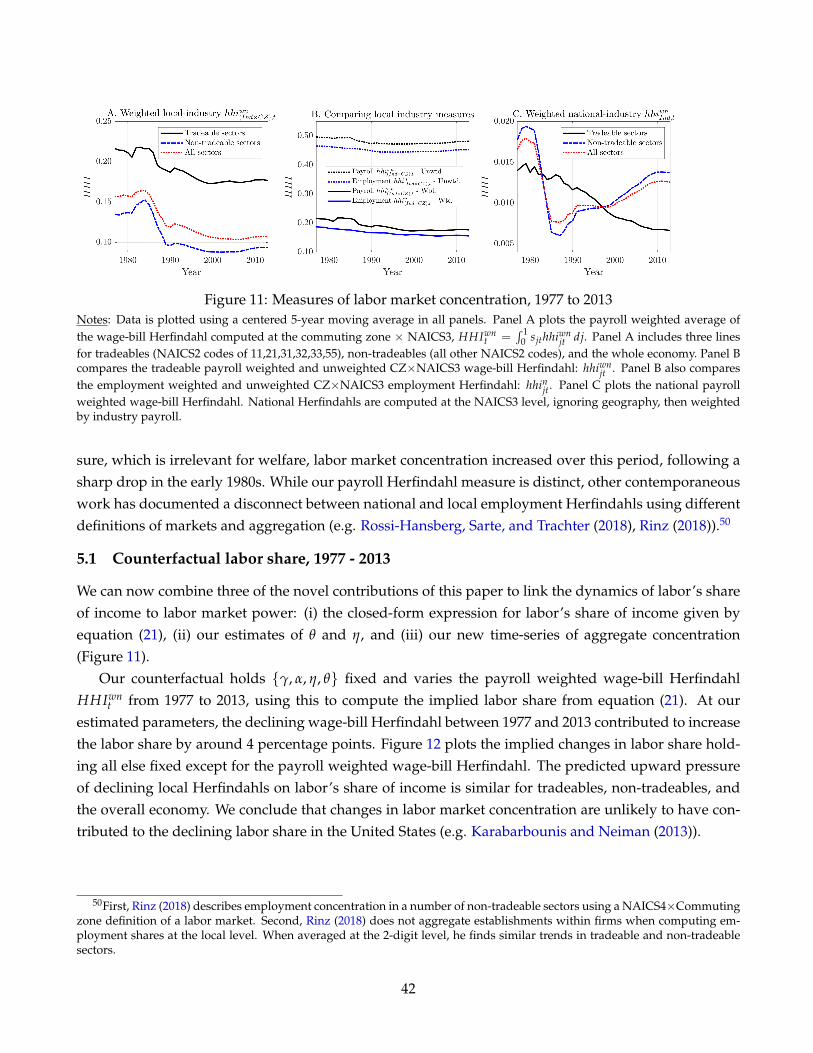
Figure 11: Measures of labor market concentration, 1977 to 2013Notes: Data is plotted using a centered 5-year moving average in all panels. Panel A plots the payroll weighted average ofthe wage-bill Herfindahl computed at the commuting zone × NAICS3, HHIwn

t =´ 1

0 sjthhiwnjt dj. Panel A includes three lines

for tradeables (NAICS2 codes of 11,21,31,32,33,55), non-tradeables (all other NAICS2 codes), and the whole economy. Panel Bcompares the tradeable payroll weighted and unweighted CZ×NAICS3 wage-bill Herfindahl: hhiwn

jt . Panel B also comparesthe employment weighted and unweighted CZ×NAICS3 employment Herfindahl: hhin

jt. Panel C plots the national payrollweighted wage-bill Herfindahl. National Herfindahls are computed at the NAICS3 level, ignoring geography, then weightedby industry payroll.

sure, which is irrelevant for welfare, labor market concentration increased over this period, following asharp drop in the early 1980s. While our payroll Herfindahl measure is distinct, other contemporaneouswork has documented a disconnect between national and local employment Herfindahls using differentdefinitions of markets and aggregation (e.g. Rossi-Hansberg, Sarte, and Trachter (2018), Rinz (2018)).50

5.1 Counterfactual labor share, 1977 - 2013

We can now combine three of the novel contributions of this paper to link the dynamics of labor’s shareof income to labor market power: (i) the closed-form expression for labor’s share of income given byequation (21), (ii) our estimates of θ and η, and (iii) our new time-series of aggregate concentration(Figure 11).

Our counterfactual holds γ, α, η, θ fixed and varies the payroll weighted wage-bill HerfindahlHHIwn

t from 1977 to 2013, using this to compute the implied labor share from equation (21). At ourestimated parameters, the declining wage-bill Herfindahl between 1977 and 2013 contributed to increasethe labor share by around 4 percentage points. Figure 12 plots the implied changes in labor share hold-ing all else fixed except for the payroll weighted wage-bill Herfindahl. The predicted upward pressureof declining local Herfindahls on labor’s share of income is similar for tradeables, non-tradeables, andthe overall economy. We conclude that changes in labor market concentration are unlikely to have con-tributed to the declining labor share in the United States (e.g. Karabarbounis and Neiman (2013)).

50First, Rinz (2018) describes employment concentration in a number of non-tradeable sectors using a NAICS4×Commutingzone definition of a labor market. Second, Rinz (2018) does not aggregate establishments within firms when computing em-ployment shares at the local level. When averaged at the 2-digit level, he finds similar trends in tradeable and non-tradeablesectors.

42

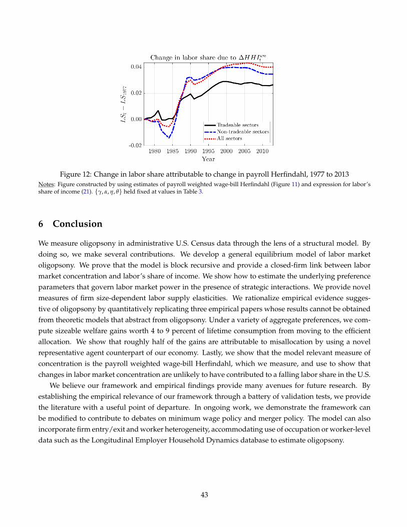
Figure 12: Change in labor share attributable to change in payroll Herfindahl, 1977 to 2013Notes: Figure constructed by using estimates of payroll weighted wage-bill Herfindahl (Figure 11) and expression for labor’sshare of income (21). γ, α, η, θ held fixed at values in Table 3.

6 Conclusion

We measure oligopsony in administrative U.S. Census data through the lens of a structural model. Bydoing so, we make several contributions. We develop a general equilibrium model of labor marketoligopsony. We prove that the model is block recursive and provide a closed-firm link between labormarket concentration and labor’s share of income. We show how to estimate the underlying preferenceparameters that govern labor market power in the presence of strategic interactions. We provide novelmeasures of firm size-dependent labor supply elasticities. We rationalize empirical evidence sugges-tive of oligopsony by quantitatively replicating three empirical papers whose results cannot be obtainedfrom theoretic models that abstract from oligopsony. Under a variety of aggregate preferences, we com-pute sizeable welfare gains worth 4 to 9 percent of lifetime consumption from moving to the efficientallocation. We show that roughly half of the gains are attributable to misallocation by using a novelrepresentative agent counterpart of our economy. Lastly, we show that the model relevant measure ofconcentration is the payroll weighted wage-bill Herfindahl, which we measure, and use to show thatchanges in labor market concentration are unlikely to have contributed to a falling labor share in the U.S.

We believe our framework and empirical findings provide many avenues for future research. Byestablishing the empirical relevance of our framework through a battery of validation tests, we providethe literature with a useful point of departure. In ongoing work, we demonstrate the framework canbe modified to contribute to debates on minimum wage policy and merger policy. The model can alsoincorporate firm entry/exit and worker heterogeneity, accommodating use of occupation or worker-leveldata such as the Longitudinal Employer Household Dynamics database to estimate oligopsony.

43

References

AMITI, M., O. ITSKHOKI, AND J. KONINGS (2014): “Importers, Exporters, and Exchange Rate Disconnect,” Ameri-can Economic Review, 104(7), 1942–78.

(2019): “International Shocks, Variable Markups, and Domestic Prices,” The Review of Economic Studies,86(6), 2356–2402.

ANDERSON, S. P., A. DE PALMA, AND J.-F. THISSE (1987): “The CES is a Discrete Choice Model?,” EconomicsLetters, 24(2), 139–140.

ARNOLD, D. (2020a): “Mergers and acquisitions, local labor market concentration, and worker outcomes,” Workingpaper.

(2020b): “Mergers and Acquisitions, Local Labor Market Concentration, and Worker Outcomes,” Discus-sion paper, UC San Diego.

ASHENFELTER, O. C., H. FARBER, AND M. R. RANSOM (2010): “Labor Market Monopsony,” Journal of LaborEconomics, 28(2), 203–210.

ATKESON, A., AND A. BURSTEIN (2008): “Pricing-to-market, trade costs, and international relative prices,” Amer-ican Economic Review, 98(5), 1998–2031.

AUTOR, D., D. DORN, L. F. KATZ, C. PATTERSON, AND J. VAN REENEN (2020): “The Fall of the Labor Share andthe Rise of Superstar Firms,” The Quarterly Journal of Economics, 135:2, 645–709.

AZAR, J., I. MARINESCU, M. STEINBAUM, AND B. TASKA (2020): “Concentration in US labor markets: Evidencefrom online vacancy data,” Labour Economics, 66, 101886.

AZAR, J., I. MARINESCU, AND M. I. STEINBAUM (2020): “Labor Market Concentration,” Journal of Human Re-sources, pp. 1218–9914R1.

AZKARATE-ASKASUA, M., AND M. ZERECERO (2020): “The Aggregate Effects of Labor Market Concentration,”Discussion paper, Working Paper.

BANFI, S., AND B. VILLENA-ROLDAN (2018): “Do high-wage jobs attract more applicants? Directed search evi-dence from the online labor market,” Journal of Labor Economics, 37(3).

BAQAEE, D. R., AND E. FARHI (2020): “Productivity and Misallocation in General Equilibrium,” The QuarterlyJournal of Economics, 135(1), 105–163.

BARKAI, S. (2020): “Declining Labor and Capital Shares,” The Journal of Finance, 75(5), 2421–2463.

BECKER, G. S. (1962): “Investment in human capital: A theoretical analysis,” Journal of Political Economy, 70(5, Part2), 9–49.

BELOT, M., P. KIRCHER, AND P. MULLER (2017): “How Wage Announcements Affect Job Search Behaviour-AField Experimental Investigation,” Working papers, European University Institute.

BENMELECH, E., N. BERGMAN, AND H. KIM (2020): “Strong Employers and Weak Employees: How Does Em-ployer Concentration Affect Wages?,” Journal of Human Resources, pp. 0119–10007R1.

44

BHASKAR, V., A. MANNING, AND T. TO (2002): “Oligopsony and monopsonistic competition in labor markets,”Journal of Economic Perspectives, 16(2), 155–174.

BLOOM, N., F. GUVENEN, B. S. SMITH, J. SONG, AND T. VON WACHTER (2018): “The Disappearing Large-FirmWage Premium,” AEA Papers and Proceedings, 108, 317–22.

BOAL, W. M., AND M. R. RANSOM (1997): “Monopsony in the Labor Market,” Journal of Economic Literature, 35(1),86–112.

BOROVICKOVA, K., AND R. SHIMER (2017): “High Wage Workers Work for High Wage Firms,” NBER WorkingPaper 24074, National Bureau of Economic Research.

BROOKS, W. J., J. P. KABOSKI, Y. A. LI, AND W. QIAN (2019): “Exploitation of Labor? Classical Monopsony Powerand Labor’s Share,” NBER Working Paper 25660, National Bureau of Economic Research.

BROWN, C., AND J. MEDOFF (1989): “The employer size-wage effect,” Journal of Political Economy, 97(5), 1027–1059.

BURDETT, K., AND D. MORTENSEN (1998): “Wage differentials, employer size, and unemployment,” InternationalEconomic Review, 39(2), 257–73.

CARD, D., A. R. CARDOSO, J. HEINING, AND P. KLINE (2018): “Firms and labor market inequality: Evidence andsome theory,” Journal of Labor Economics, 36(S1), 13–70.

CHAN, M., S. SALGADO, AND M. XU (2020): “Heterogeneous Passthrough from TFP to Wages,” Available at SSRN3538503.

DE LOECKER, J., J. EECKHOUT, AND G. UNGER (2020): “The Rise of Market Power and the Macroeconomic Impli-cations,” The Quarterly Journal of Economics, 135(2), 561–644.

DELGADO, M., R. BRYDEN, AND S. ZYONTZ (2014): “Categorization of traded and local industries in the USeconomy,” Discussion paper, Mimeo. Available online at: http://www. clustermapping. us/[Accessed May2015].

DERENONCOURT, E., C. NOELKE, AND D. WEIL (2021): “Spillover Effects from Voluntary Employer MinimumWages,” Available at SSRN 3793677.

DUBE, A., D. CENGIZ, A. LINDNER, AND B. ZIPPERER (2019): “The Effect of Minimum Wages on Low-WageJobs,” Quarterly Journal of Economics, 134(3).

DUBE, A., J. JACOBS, S. NAIDU, AND S. SURI (2020): “Monopsony in Online Labor Markets,” American EconomicReview: Insights, 2(1), 33–46.

EDMOND, C., V. MIDRIGAN, AND D. Y. XU (2018): “How Costly Are Markups?,” NBER Working Paper 24800,National Bureau of Economic Research.

FORT, T. C., AND S. D. KLIMEK (2018): “The Effects of Industry Classification Changes on US Employment Com-position,” Working Papers 18-28, Center for Economic Studies, U.S. Census Bureau.

FRIEDRICH, B., L. LAUN, C. MEGHIR, AND L. PISTAFERRI (2019): “Earnings Dynamics and Firm-Level Shocks,”NBER Working Paper 25786, National Bureau of Economic Research.

45

GIROUD, X., AND J. RAUH (2019): “State Taxation and the Reallocation of Business Activity: Evidence fromEstablishment-Level Data,” Journal of Political Economy, 127(3).

GUTIÉRREZ, G., AND T. PHILIPPON (2017): “Declining Competition and Investment in the U.S.,” Working Paper23583, National Bureau of Economic Research.

HANDWERKER, E. W., AND M. DEY (2018): “Megafirms and Monopsonists: Not the same employers, not the sameworkers,” BLS Working Paper Series, 2.

HERSHBEIN, B., C. MACALUSO, AND C. YEH (2020): “Monopsony in the U.S. labor market,” Discussion paper,Working paper.

HOPENHAYN, H. A. (1992): “Entry, Exit, and firm Dynamics in Long Run Equilibrium,” Econometrica, 60(5), 1127–1150.

HOTELLING, H. (1990): “Stability in competition,” in The Collected Economics Articles of Harold Hotelling, pp. 50–63.Springer.

JAROSCH, G., J. S. NIMCSIK, AND I. SORKIN (2019): “Granular Search, Market Structure, and Wages,” NBERWorking Paper 26239, National Bureau of Economic Research.

KARABARBOUNIS, L., AND B. NEIMAN (2013): “The Global Decline of the Labor Share,” The Quarterly Journal ofEconomics, 129(1), 61–103.

KEHRIG, M., AND N. VINCENT (2021): “The Micro-Level Anatomy of the Labor Share Decline,” The QuarterlyJournal of Economics, 136(2), 1031–1087.

KENNAN, J., AND J. R. WALKER (2011): “The effect of expected income on individual migration decisions,” Econo-metrica, 79(1), 211–251.

KLINE, P., N. PETKOVA, H. WILLIAMS, AND O. ZIDAR (2019): “Who Profits from Patents? Rent-Sharing at Inno-vative Firms,” Quarterly Journal of Economics, 134(3), 1343–404.

KROFT, K., Y. LUO, M. MOGSTAD, AND B. SETZLER (2020): “Imperfect Competition and Rents in Labor andProduct Markets: The Case of the Construction Industry,” Discussion paper, National Bureau of EconomicResearch.

LALLEMAND, T., R. PLASMAN, AND F. RYCX (2007): “The Establishment-size Wage Premium: Evidence fromEuropean Countries,” Empirica, 34(5), 427–451.

LAMADON, T., M. MOGSTAD, AND B. SETZLER (2019): “Imperfect Competition and Rent Sharing in the U.S. LaborMarket,” NBER Working Paper 25954, National Bureau of Economic Research.

MACKENZIE, G. (2019): “Trade and market power in product and labor markets,” Unpublished Working Paper.

MALMBERG, H. (2013): “Random Choice over a Continuous Set of Options,” Ph.D. thesis, Department of Mathe-matics, Stockholm University.

MANNING, A. (2003): Monopsony in motion: Imperfect competition in labor markets. Princeton University Press.

46

(2011): “Imperfect Competition in the Labor Market,” in Handbook of labor economics, vol. 4, pp. 973–1041.Elsevier.

MITMAN, K., AND S. RABINOVICH (2019): “Do Changes in Unemployment Insurance Explain the Emergence ofJobless Recoveries?,” Discussion Paper Series ZA DP No. 12365, IZA Institute of Labor Economics.

RINZ, K. (2018): “Labor Market Concentration, Earnings Inequality, and Earnings Mobility,” CARRA WorkingPaper Series 2018-10, Center for Administrative Records Research and Applications , US Census Bureau.

ROBINSON, J. (1933): The Economics of Imperfect Competition. Palgrave Macmillan.

ROSSI-HANSBERG, E., P.-D. SARTE, AND N. TRACHTER (2018): “Diverging Trends in National and Local Concen-tration,” NBER Working Paper 25066, National Bureau of Economic Research.

SALOP, S. C. (1979): “Monopolistic Competition with Outside Goods,” The Bell Journal of Economics, pp. 141–156.

STAIGER, D. O., J. SPETZ, AND C. S. PHIBBS (2010): “Is There Monopsony in the Labor Market? Evidence from aNatural Experiment,” Journal of Labor Economics, 28(2), 211–236.

SUÁREZ SERRATO, J. C., AND O. ZIDAR (2016): “Who Benefits from State Corporate Tax Cuts? A Local LaborMarkets Approach with Heterogeneous Firms,” American Economic Review, 106(9), 2582–2624.

VERBOVEN, F. (1996): “The nested logit model and representative consumer theory,” Economics Letters, 50(1), 57–63.

WEBBER, D. A. (2015): “Firm market power and the earnings distribution,” Labour Economics, 35, 123–134.

WEBBER, D. A. (2016): “Firm-Level Monopsony and the Gender Pay Gap,” Industrial Relations: A Journal of Econ-omy and Society, 55(2), 323–345.

47

APPENDIX FOR ONLINE PUBLICATION

This Appendix is organized as follows. Section A provides additional tables and figures references in the text. Section Bprovides our micro-foundation for nested-CES preferences used in the main text and references in Section 1. Section C containsdetails about the data and sample selection criteria. Section D contains summary statistics used and references in the paper andadditional concentration measures. Section E contains derivations of all mathematical expressions in the text, including proofsof Propositions. Section F provides additional details regarding the calibration. Section G provides additional discussion of ourempirical results and robustness on a number of dimensions.

A Additional tables and figures

Description Model Data (KPZW)

Log change in VAPW (VAPW=Zzijnα−1ij ) 0.13 0.13

Median firm size 34.59 25.26Mean firm size 61.85 61.49Median VAPW (dollars) 57152 86870Mean VAPW (dollars) 57716 120160

Model Simulation Parameters

Size cutoff (Employees) 11.00Fraction of Firms Shocked 0.01Shock size (dlog(zij)) 0.17

Table A1: Wage pass-through experiment detailsNotes: Summary statistics for replication of Kline, Petkova, Williams, and Zidar (2019) regressions. We randomly sample onepercent of firms in our benchmark economy. We draw firms with employment greater than n. We increase the productivity oftreated firms by a factor ∆logzi j. The values of n and ∆ are calibrated to match the KPWZ (1) median firm size of 25 employees,(2) increase in post-tax value added per worker of 13 percent. We keep aggregates fixed and solve the new market equilibrium.

We treat the untreated and treated observations for each firm as a panel with two observations per firm of wages

wij0, wij1

and value added per worker,

yij0nij0

, yij1nij1

. We then regress the wages in levels on VAPW in levels and a firm-specific fixed effect.

The regression coefficient is converted into an elasticity using untreated mean wages and mean value added per worker.

48

Model Data

Wage bill Herfindahl – Payroll weighted average 0.17 0.17

Wage bill Herfindahl – Unweighted average 0.33 0.48

Wage bill Herfindahl correlation with market employment -0.86 -0.25

Employment Herfindahl – Payroll weighted average 0.15 0.15

Employment Herfindahl – Unweighted average 0.32 0.45

Employment Herfindahl correlation with Wage-bill Herfindahl 1.00 0.98

Table A2: Concentration and competition, model versus dataNotes: Data is from 2014 LBD, tradeable sectors. Model is for tradeable calibration. The market level wage-bill Herfindahl is

given by: HHIwnj := ∑i∈j

(swn

ij

)2, swn

ij =wijnij

∑i∈j wijnij. When aggregating, we weight by the market’s payroll share sj =

∑i∈j wijnij´∑i∈j wijnijdj

so that HHIwn =´

sj HHIwnj dj. The market level employment Herfindahl is given by: HHIn

j := ∑i∈j

(sn

ij

)2, sn

ij =nij

∑i∈j nij. We

weight the market level employment Herfindahls similarly.

Figure A1: Cross market distribution of concentration model v. data

Notes: This figure plots the market-level distribution of the payroll Herindahl index (HHIwnj ). Model corresponds to the all

sectors model. Bins are determined by the following bounds: 0, 0.25, 0.50, 0.75, 0.99, 1. The horizontal axis gives the centerof each bin. Panel (i) plots the fraction of total payroll in each bin. Panel (ii) plots the fraction of markets in each bin. Data isCensus LBD. See Appendix C for additional details.

49

Labor Supply Elasticity Industry Gender Country (Region) Paper Table/Page

1.31 Agriculture US Weber(2018) Table41.6 Mining/oil/natural gas US Weber(2018) Table41.4 Utility US Weber(2018) Table41.59 Construction US Weber(2018) Table41.72 Manufacturing US Weber(2018) Table41.52 Wholesale trade US Weber(2018) Table41.07 Resale trade US Weber(2018) Table41.45 Transportation US Weber(2018) Table41.22 Information US Weber(2018) Table41.38 Finance and insurance US Weber(2018) Table41.13 Real estate and rental US Weber(2018) Table41.3 Profession/Scientific/technical services US Weber(2018) Table41 Management of companies US Weber(2018) Table40.97 Administrative support US Weber(2018) Table40.96 Educaitonal Services US Weber(2018) Table40.97 Health Care and Social Assistance US Weber(2018) Table40.93 Art and entertainment US Weber(2018) Table40.96 Accommodation and food services US Weber(2018) Table51.19 Other services US Weber(2018) Table51.11 Public administration US Weber(2018) Table53.7 Public school teachers US Ransom and Sims(2010) Table54.6 Retail stores US Dube et all(2019) Table51.43 Agriculture US Weber(2015) Table51.52 Mining/oil/natural gas US Weber(2015) Table51.18 Utility US Weber(2015) Table51.42 Construction US Weber(2015) Table51.82 Manufacturing US Weber(2015) Table51.48 Wholesale trade US Weber(2015) Table51.03 Resale trade US Weber(2015) Table51.47 Transportation US Weber(2015) Table51.17 Information US Weber(2015) Table51.27 Finance and insurance US Weber(2015) Table51.01 Real estate and rental US Weber(2015) Table51.17 Profession/Scientific/technical services US Weber(2015) Table51.17 Management of companies US Weber(2015) Table50.72 Administrative support US Weber(2015) Table50.91 Educaitonal Services US Weber(2015) p10.78 Health Care and Social Assistance US Weber(2015) p260.94 Art and entertainment US Weber(2015) p10.85 Accomodation and food services US Weber(2015) p301.04 Other services US Weber(2015) p11.19 Public administration US Weber(2015) Table91.09 All US Weber(2016) Table90.94 All US Weber(2016) Table91.86 Manufacture Skilled (Market FE) US Tortarolo and Zarate (2020) p14 Manufacture Unskilled (Market FE) US Tortarolo and Zarate (2020) p12.74 Manufacture All US Tortarolo and Zarate (2020) p10.1 Nurse at VA US Staiger et all(2010) Table70.1 Amazon Online Task Market US Dube et all(2020) Table52.7 Retail stores US Ransom and Oaxaca(2010) Table51.5 Retail stores US Ransom and Oaxaca(2010) Table53.94 Ford US Depew and Sorensen(2013) p62.52 Byers US Depew and Sorensen(2013) p62.37 Documented US Hotchkiss and Quispe-Agnoli(2012) Table21.85 Undocumented US Hotchkiss and Quispe-Agnoli(2013) Table32.574 All US Dobbelaere and Mairesse(2013) Table5

Table A3: Meta-analysis: US Data

50

Labor Supply Elasticity Industry Gender Country (Region) Paper Table/Page

0.71 All Australia Booth and Katic(2011) p12.175 All(rais) Brazil Vick(2017) Table71.502 All(rais) Brazil Vick(2017) Table71.292 Agriculture East Germany Bachmann and Fringes (2017) Table72.28 Mining and utilities East Germany Bachmann and Fringes (2017) Table72.482 Manufacturing of food products East Germany Bachmann and Fringes (2017) Table73.369 Manufacturing of consumer products East Germany Bachmann and Fringes (2017) Table71.343 Manufactuying of industial products East Germany Bachmann and Fringes (2017) Table72.507 Manufacturing of capital goods East Germany Bachmann and Fringes (2017) Table72.762 Construction East Germany Bachmann and Fringes (2017) Table70.717 Wholesale East Germany Bachmann and Fringes (2017) Table70.344 Retailing East Germany Bachmann and Fringes (2017) Table71.427 Transportation East Germany Bachmann and Fringes (2017) Table7-1.095 Hotel and restaurants East Germany Bachmann and Fringes (2017) Table71.794 Financial services East Germany Bachmann and Fringes (2017) Table71.896 Liberal professions East Germany Bachmann and Fringes (2017) Table72.918 Education East Germany Bachmann and Fringes (2017) Table72.109 Health East Germany Bachmann and Fringes (2017) Table72.786 Other services East Germany Bachmann and Fringes (2017) Table70.932 Nonindustrial organization East Germany Bachmann and Fringes (2017) Table71.563 Public administration East Germany Bachmann and Fringes (2017) p11.788 All East Germany Bachmann and Fringes (2017) p13.072 All Germany Hirsch, Schank and Schnabel (2010a) Table42.225 All Germany Hirsch, Schank and Schnabel (2010a) Table41.875 Foreigner Germany Hirsch, Jahn(2012) p341.645 Germans Germany Hirsch, Jahn(2012) p342.044 All Germany Hirsch, Schank and Schnabel (2013) Table30.52 All Indonesia Brummund(2011) Table50.4 All Italy Sulis et all (2011) Table90.307 All Italy Sulis et all (2011) Table92.15 Public Sector Mexico Bo, Finan and Rossi(2013) p31.4 Teacher Norway Falch(2010) Table51.25 Teacher Norway Falch(2011) p61.4 Teacher Norway Falch(2017) p11.41 All(Foreign Workers) United Arab Emirates Naidu, Nyarko and Wang(2014) Table50.883 Agriculture West Germany Bachmann and Fringes (2017) p12.577 Mining and utilities West Germany Bachmann and Fringes (2017) Table32.227 Manufacturing of food products West Germany Bachmann and Fringes (2017) Table31.757 Manufacturing of consumer products West Germany Bachmann and Fringes (2017) p62.249 Manufactuying of industial products West Germany Bachmann and Fringes (2017) p62.841 Manufacturing of capital goods West Germany Bachmann and Fringes (2017) Table52.167 Construction West Germany Bachmann and Fringes (2017) Table51.728 Wholesale West Germany Bachmann and Fringes (2017) Table50.737 Retailing West Germany Bachmann and Fringes (2017) Table52.178 Transportation West Germany Bachmann and Fringes (2017) Table50.274 Hotel and restaurants West Germany Bachmann and Fringes (2017) Table52.526 Financial services West Germany Bachmann and Fringes (2017) Table52.473 Liberal professions West Germany Bachmann and Fringes (2017) Table53.498 Education West Germany Bachmann and Fringes (2017) Table51.407 Health West Germany Bachmann and Fringes (2017) Table51.445 Other services West Germany Bachmann and Fringes (2017) Table51.607 Nonindustrial organization West Germany Bachmann and Fringes (2017) Table51.597 Public administration West Germany Bachmann and Fringes (2017) Table52.021 All West Germany Bachmann and Fringes (2017) Table5

Table A4: Meta-analysis: Non-US data

51

Figure A2: Oligopsonistic equilibrium with varying decreasing returns α

Notes: Figure constructed from model under estimated parameters (Table 3). Low, medium and high productivities of thefirms correspond to the 10th, 50th and 90th percentiles of the productivity distribution.

Figure A3: Oligopsonistic vs. Competitive equilibriumNotes: In a oligopsonistic equilibrium (Panel A) the firm understands that its marginal cost MCij is increasing in its employment.In a competitive equilibrium (Panel B) the firm perceives that its marginal cost MCij is simply equal to its wage, which it takes asgiven. The true labor supply curve to the firm, however, is still upward sloping, reflecting household preferences.

52

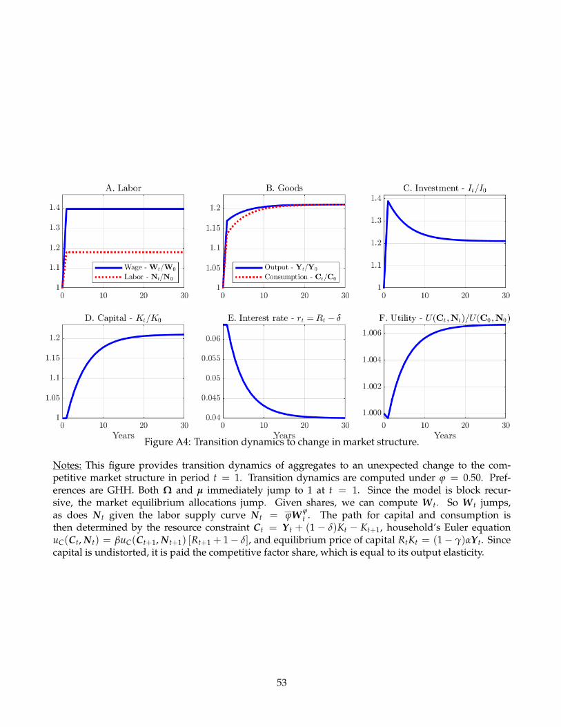
Figure A4: Transition dynamics to change in market structure.

Notes: This figure provides transition dynamics of aggregates to an unexpected change to the com-petitive market structure in period t = 1. Transition dynamics are computed under ϕ = 0.50. Pref-erences are GHH. Both Ω and µ immediately jump to 1 at t = 1. Since the model is block recur-sive, the market equilibrium allocations jump. Given shares, we can compute W t. So W t jumps,as does N t given the labor supply curve N t = ϕW ϕ

t . The path for capital and consumption isthen determined by the resource constraint Ct = Y t + (1 − δ)Kt − Kt+1, household’s Euler equationuC(Ct, N t) = βuC(Ct+1, N t+1) [Rt+1 + 1− δ], and equilibrium price of capital RtKt = (1− γ)αY t. Sincecapital is undistorted, it is paid the competitive factor share, which is equal to its output elasticity.

53

B Microfounding the nested CES labor supply system

In this section we provide a micro-foundation for the nested CES preferences used in the main text. The arguments used hereadapt those in Verboven (1996). We begin with the case of monopsonistic competition to develop ideas and then move to thecase of oligopsonistic labor markets studied in the text. We then show that the same supply system occurs in a setting whereworkers solve a dynamic discrete choice problem and firms compete in a dynamic oligopoly.

B.1 Static discrete choice framework

Agents. There is a unit measure of ex-ante identical individuals indexed by l ∈ [0, 1]. There is a large but finite set of Jsectors in the economy, with finitely many firms i ∈ 1, . . . , Mj in each sector.

Preferences. Each individual has random preferences for working at each firm ij. Their disutility of labor supply is convexin hours worked hl . Worker l’s disutility of working hlij hours at firm ij are:

νlij = e−µξlij hlij , log νlij = log hij − µξij,

where the random utility term ξlij is distributed iid across individuals according from a multi-variate Gumbel distribution:

F(ξi1, ..., ξNJ) = exp

−∑ij

e−(1+η)ξij

.

The term ξlij is a worker-firm specific term which reduces labor disutility and hence could capture (i) an inverse measure ofcommuting costs, or (ii) a positive amenity.

Decisions. Each individual must earn yl ∼ F (y), where earnings yl = wijhlij. After drawing their vector

ξlij

, each

worker solvesmin

ij

log hij − ξlij

≡ max

ij

log wij − log yl + ξlij

.

This problem delivers the following probability that worker l chooses to work at firm ij, which is independent of yl :

Probl

(wij, w−ij

)=

w1+ηij

∑ij w1+ηij

. (B1)

Aggregation. Total labor supply to firm ij, is then found by integrating these probabilities, multiplied by the hours sup-plied by each worker l:

nij =

ˆ 1

0Probl

(wij, w−ij

)hlijdF (yl) , hlij = yl/wij

nij =wη

ij

∑i∈j w1+ηij

ˆ 1

0yldF (yl)︸ ︷︷ ︸

:=Y

(B2)

Aggregating this expression we obtain the obvious result that ∑i∈j wijnij = Y. Now define the following indexes:

W :=

∑i∈j

w1+ηij

11+η

, N :=

∑i∈j

nη+1

η

ij

η

η+1

.

54

Along with (B2), these indexes imply that W N = Y. Using these definitions along with W N = Y in (B2) yields the CES supplycurve:

nij =

(wij

W

)η

N.

We therefore have the result that the supply curves that face firms in this model of individual discrete choice are equivalent tothose that face the firms when a representative household solves the following income maximization problem:

maxnij

∑i∈j

wijnij s.t.

∑i∈j

nη+1

η

ij

η

η+1

= N.

Since at the solution, the objective function is equal to W N, then the envelope condition delivers a natural interpretation of Was the equilibrium payment to total labor input in the economy for one additional unit of aggregate labor disutility. That is, thefollowing equalities hold:

∂

∂N ∑i∈j

wijn∗ij(wij, w−ij) = Λ = W =∂

∂NW N.

Nested logit and nested CES. Consider changing the distribution of preference shocks as follows:

F(ξi1, ..., ξNJ) = exp

− J

∑j=1

(Mj

∑i=1

e−(1+η)ξij

) 1+θ1+η

.

We recover the distribution (B1) above if η = θ. Otherwise, if η > θ the problem is convex and the conditional covariance ofwithin sector preference draws differ from the economy wide variance of preference draws. We discuss this more below.

In this setting, choice probabilities can be expressed as the product of the conditional choice probability of supplying laborto firm i conditional on supplying labor to market j, and the probability of supplying labor to market j:

Probl

(wij, w−ij

)=

w1+ηij

∑Mj

i=1 w1+ηij︸ ︷︷ ︸

Probl(Choose firm i|Choose market j)

×

[∑

Mj

i=1 w1+ηij

] 1+θ1+η

∑Jl=1

[∑Ml

k=1 w1+ηkl

] 1+θ1+η︸ ︷︷ ︸

Probl(Choose market j)

.

Following the same steps as above, we can aggregate these choice probabilities and hours decisions to obtain firm level laborsupply:

nij =wη

ij

∑Mj

i=1 w1+ηij

[∑

Mj

i=1 w1+ηij

] 1+θ1+η

∑Jl=1

[∑Ml

k=1 w1+ηkl

] 1+θ1+η

Y. (B3)

We can now define the following indexes:

W j =

[Mj

∑i=1

w1+ηij

] 11+η

, N j =

[Mj

∑i=1

n1+η

η

ij

] η1+η

,

W =

J

∑j=1

W1+θj

11+θ

, N =

J

∑j=1

N1+θ

θ

j

θ1+θ

.

Using these definitions and similar results to the above we can show that W j N j = ∑Mj

i=1 wijnij, and Y = W N = ∑Jj=1 W j N j.

Consider the thought experiment of adding more markets J (which is necessary to identically map these formulas to ourmodel). While the min of an infinite number of draws from a Gumbel distribution is not defined (it asymptotes to −∞), thedistribution of choices across markets is defined at each point in the limit as we add more markets J (Malmberg, 2013). As a

55

result, the distribution of choices will have a well defined limit, and with the correct scaling as we add more markets (we canscale the disutilities at each step and not affect the market choice), as described in (Malmberg, 2013), the limiting wage indexeswill be defined as above. We can then express (B3) as:

nij =

(wij

W j

)η (W j

W

)θ

N,

which completes the CES supply system defined in the text.

Comment. The above has established that it is straightforward to derive the supply system in the model through a dis-crete choice framework. This is particularly appealing given recent modeling of labor supply using familiar discrete choiceframeworks first in models of economic geography and more recently in labor (Borovickova and Shimer (2017), Card, Car-doso, Heining, and Kline (2018), Lamadon, Mogstad, and Setzler (2019)). Since firms take this supply system as given, wecan then work with the nested CES supply functions as if they were derived from the preferences and decisions of a represen-tative household. This vastly simplifies welfare computations and allows for the integration of the model into more familiarmacroeconomic environments.

The second advantage of this micro-foundation is that it provides a natural interpretation of the somewhat nebulouselasticities of substitution in the CES specification: η and θ. Returning to the Gumbel distribution we observe the following

F(ξi1, ..., ξNJ) = exp

− J

∑j=1

(Mj

∑i=1

e−(1+η)ξij

) 1+θ1+η

A higher value of η increases the correlation of draws within a market (McFadden, 1978). Within a market if η is high, then anindividual’s preference draws are likely to be clustered. With little difference in non-pecuniary idiosyncratic preferences forworking at different firms, wages dominate in an individual’s labor supply decision and wage posting in the market is closerto the competitive outcome. A higher value of θ decreases the overall variance of draws across all firms (i.e. it increases thecorrelation across any two randomly chosen sub-vectors of an individual’s draws). An individual is therefore more likely tofind that their lowest levels of idiosyncratic disutility are in two different markets, increasing across market wage competition.

In the case that η = θ, the model collapses to the standard logit model. In this case the following obtains. Take anindividual’s ξlij for some firm. The conditional probability distribution of some other draw ξli′ j′ is the same whether firm i′ isin the same market (j′ = j) or some other market (j′ 6= j). Individuals are as likely to find somewhere local that incurs the samelevel of labor disability as finding somewhere in another market. In this setting economy-wide monopsonistic competitionobtains. When an individual is more likely to find their other low disutility draws in the same market, then firms within thatmarket have local market power. This is precisely the case that obtains when η > θ.

B.2 Dynamic discrete choice framework

We show that the above discrete choice framework can be adapted to an environment where some individuals draw newvectors ξl each period and reoptimize their labor supply. Firms therefore compete in a dynamic oligopoly. Restricting attentionto the stationary solution of the model where firms keep employment and wages constant—as in the tradition of Burdettand Mortensen (1998)—we show that the allocation of employment and wages once again coincide with the solution to theproblem in the main text. To simplify notation we consider the problem for a market with M firms i ∈ 1, . . . , M which maybe generalized to the model in the text.

Environment. Every period a random fraction λ of workers each draw a new vector ξl . Let ni be employment at firm i.Let wi be the average wage of workers at firm i, such that the total wage bill in the firm is wini. Let the equilibrium labor supplyfunction h(wi, w−i) determine the amount of hires a firm makes if it posts a wage wi when its competitors’ wages in the marketare given by the vector w−i.

56

Value function. Let V(ni, wi) be the firm’s present discounted value of profits, where the firm has discount rate β = 1.Then V(ni, wi) satisfies:

V (ni, wi) = (Pzi − wi) (1− λ) ni + maxw′i

(Pzi − w′i

)h(w′i , w′−i

)+ V

(n′i , w′i

), (B4)

n′(ni, w′i , w′−i

)= (1− λ) ni + h

(w′i , w′−i

), (B5)

w′(ni, wi, w′i , w′−i

)=

(1− λ)wini + h(

w′i , w′−i

)w′i

(1− λ) ni + h(

w′i , w′−i

) . (B6)

The firm operates a constant returns to scale production function. Of the firm’s ni workers, a fraction (1− λ) do not draw newpreferences. The total profit associated with these workers is then average revenue (Pzi) minus average cost (wi). The firmchooses a new wage w′i to post in the market. In equilibrium, given its competitor’s wages w′−i, it hires h(w′i , w′−i) workers.The total profit associated with these workers is again average revenue (Pzi) minus average cost (w′i). The second and thirdequations account for the evolution of the firm’s state variables.

Optimality. Given its competitor’s prices, the first order condition with respect to w′i is:(Pzi − w′i

)h1(w′i , w′−i

)− h

(w′i , w′−i

)+ Vn

(n′i , w′i

)n′w(ni, w′i , w′−i

)+ Vw

(n′i , w′i

)ww(ni, wi, w′i , w′−i

)= 0

The relevant envelope conditions are

Vn (ni, wi) = (Pzi − wi) (1− λ) + Vn(n′i , w′i

)n′n(ni, w′i , w′−i

)+ Vw

(n′i , w′i

)w′n(ni, wi, w′i , w′−i

)Vw (ni, wi) = − (1− λ) ni + Vw

(n′i , w′i

)w′w(ni, wi, w′i , w′−i

)In a stationary equilibrium wi = w′i , and n′i = ni. One can compute the partial derivatives involved in these expressions, andevaluate the conditions under stationarity to obtain

(Pzi − wi) h1 (wi, w−i) = h (wi, w−i) .

Rearranging this expression:

wi =εi(wi, w−i)

εi(wi, w−i) + 1Pzi , εi(wi, w−i) :=

h1(wi, w−i)wih(wi, w−i)

The solution to the dynamic oligopsony problem for a given supply system is identical to the solution of the static problem. Inthis setting, the supply system is obviously that which is obtained from the individual discrete choice problem in the previoussection.

Comments. This setting establishes that the model considered in the main text can also be conceived as a setting whereindividuals periodically receive some preference shock that causes them to relocate, and firms engage in a dynamic oligopolygiven these worker decisions. When η > θ the shock causes a worker to consider all firms in one market very carefully to theexclusion of other markets when they are making their relocation decision. When η = θ the individual considers all firms in allmarkets equally.

57

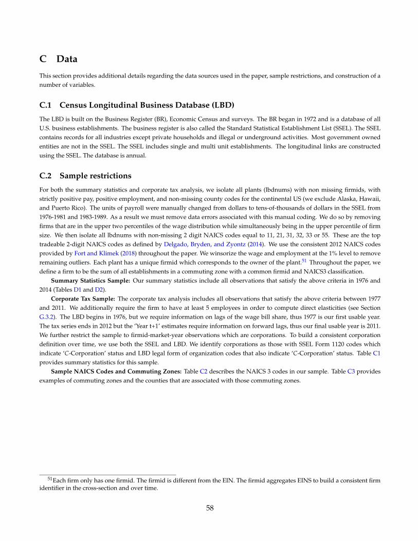
C Data

This section provides additional details regarding the data sources used in the paper, sample restrictions, and construction of anumber of variables.

C.1 Census Longitudinal Business Database (LBD)

The LBD is built on the Business Register (BR), Economic Census and surveys. The BR began in 1972 and is a database of allU.S. business establishments. The business register is also called the Standard Statistical Establishment List (SSEL). The SSELcontains records for all industries except private households and illegal or underground activities. Most government ownedentities are not in the SSEL. The SSEL includes single and multi unit establishments. The longitudinal links are constructedusing the SSEL. The database is annual.

C.2 Sample restrictions

For both the summary statistics and corporate tax analysis, we isolate all plants (lbdnums) with non missing firmids, withstrictly positive pay, positive employment, and non-missing county codes for the continental US (we exclude Alaska, Hawaii,and Puerto Rico). The units of payroll were manually changed from dollars to tens-of-thousands of dollars in the SSEL from1976-1981 and 1983-1989. As a result we must remove data errors associated with this manual coding. We do so by removingfirms that are in the upper two percentiles of the wage distribution while simultaneously being in the upper percentile of firmsize. We then isolate all lbdnums with non-missing 2 digit NAICS codes equal to 11, 21, 31, 32, 33 or 55. These are the toptradeable 2-digit NAICS codes as defined by Delgado, Bryden, and Zyontz (2014). We use the consistent 2012 NAICS codesprovided by Fort and Klimek (2018) throughout the paper. We winsorize the wage and employment at the 1% level to removeremaining outliers. Each plant has a unique firmid which corresponds to the owner of the plant.51 Throughout the paper, wedefine a firm to be the sum of all establishments in a commuting zone with a common firmid and NAICS3 classification.

Summary Statistics Sample: Our summary statistics include all observations that satisfy the above criteria in 1976 and2014 (Tables D1 and D2).

Corporate Tax Sample: The corporate tax analysis includes all observations that satisfy the above criteria between 1977and 2011. We additionally require the firm to have at least 5 employees in order to compute direct elasticities (see SectionG.3.2). The LBD begins in 1976, but we require information on lags of the wage bill share, thus 1977 is our first usable year.The tax series ends in 2012 but the ‘Year t+1’ estimates require information on forward lags, thus our final usable year is 2011.We further restrict the sample to firmid-market-year observations which are corporations. To build a consistent corporationdefinition over time, we use both the SSEL and LBD. We identify corporations as those with SSEL Form 1120 codes whichindicate ‘C-Corporation’ status and LBD legal form of organization codes that also indicate ‘C-Corporation’ status. Table C1provides summary statistics for this sample.

Sample NAICS Codes and Commuting Zones: Table C2 describes the NAICS 3 codes in our sample. Table C3 providesexamples of commuting zones and the counties that are associated with those commuting zones.

51Each firm only has one firmid. The firmid is different from the EIN. The firmid aggregates EINS to build a consistent firmidentifier in the cross-section and over time.

58

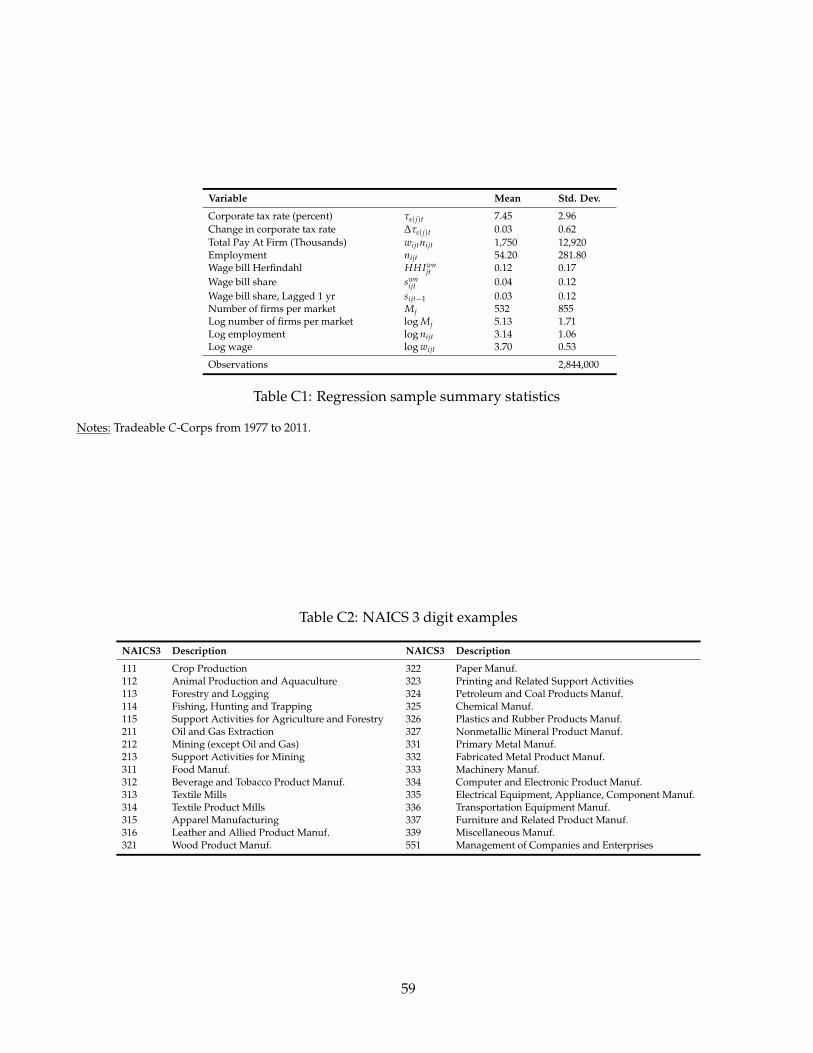
Variable Mean Std. Dev.

Corporate tax rate (percent) τs(j)t 7.45 2.96Change in corporate tax rate ∆τs(j)t 0.03 0.62Total Pay At Firm (Thousands) wijtnijt 1,750 12,920Employment nijt 54.20 281.80Wage bill Herfindahl HHIwn

jt 0.12 0.17Wage bill share swn

ijt 0.04 0.12Wage bill share, Lagged 1 yr sijt−1 0.03 0.12Number of firms per market Mj 532 855Log number of firms per market log Mj 5.13 1.71Log employment log nijt 3.14 1.06Log wage log wijt 3.70 0.53

Observations 2,844,000

Table C1: Regression sample summary statistics

Notes: Tradeable C-Corps from 1977 to 2011.

Table C2: NAICS 3 digit examples

NAICS3 Description NAICS3 Description

111 Crop Production 322 Paper Manuf.112 Animal Production and Aquaculture 323 Printing and Related Support Activities113 Forestry and Logging 324 Petroleum and Coal Products Manuf.114 Fishing, Hunting and Trapping 325 Chemical Manuf.115 Support Activities for Agriculture and Forestry 326 Plastics and Rubber Products Manuf.211 Oil and Gas Extraction 327 Nonmetallic Mineral Product Manuf.212 Mining (except Oil and Gas) 331 Primary Metal Manuf.213 Support Activities for Mining 332 Fabricated Metal Product Manuf.311 Food Manuf. 333 Machinery Manuf.312 Beverage and Tobacco Product Manuf. 334 Computer and Electronic Product Manuf.313 Textile Mills 335 Electrical Equipment, Appliance, Component Manuf.314 Textile Product Mills 336 Transportation Equipment Manuf.315 Apparel Manufacturing 337 Furniture and Related Product Manuf.316 Leather and Allied Product Manuf. 339 Miscellaneous Manuf.321 Wood Product Manuf. 551 Management of Companies and Enterprises

59

Table C3: Commuting Zone (CZ) examples: Census commuting zones numbers 58 and 47

CZ ID, 2000 County Name Metro. Area, 2003 County Pop. 2000 CZ Pop. 2000

58 Cook County Chicago-Naperville-Joliet, IL Metro. Division 5,376,741 8,704,93558 DeKalb County Chicago-Naperville-Joliet, IL Metro. Division 88,969 8,704,93558 DuPage County Chicago-Naperville-Joliet, IL Metro. Division 904,161 8,704,93558 Grundy County Chicago-Naperville-Joliet, IL Metro. Division 37,535 8,704,93558 Kane County Chicago-Naperville-Joliet, IL Metro. Division 404,119 8,704,93558 Kendall County Chicago-Naperville-Joliet, IL Metro. Division 54,544 8,704,93558 Lake County Lake County-Kenosha County, IL-WI Metro. Division 644,356 8,704,93558 McHenry County Chicago-Naperville-Joliet, IL Metro. Division 260,077 8,704,93558 Will County Chicago-Naperville-Joliet, IL Metro. Division 502,266 8,704,93558 Kenosha County Lake County-Kenosha County, IL-WI Metro. Division 149,577 8,704,93558 Racine County Racine, WI MSA 188,831 8,704,93558 Walworth County Whitewater, WI Micropolitan SA 93,759 8,704,935

47 Anoka County Minneapolis-St. Paul-Bloomington, MN-WI MSA 298,084 2,904,38947 Carver County Minneapolis-St. Paul-Bloomington, MN-WI MSA 70,205 2,904,38947 Chisago County Minneapolis-St. Paul-Bloomington, MN-WI MSA 41,101 2,904,38947 Dakota County Minneapolis-St. Paul-Bloomington, MN-WI MSA 355,904 2,904,38947 Hennepin County Minneapolis-St. Paul-Bloomington, MN-WI MSA 1,116,200 2,904,38947 Isanti County Minneapolis-St. Paul-Bloomington, MN-WI MSA 31,287 2,904,38947 Ramsey County Minneapolis-St. Paul-Bloomington, MN-WI MSA 511,035 2,904,38947 Scott County Minneapolis-St. Paul-Bloomington, MN-WI MSA 89,498 2,904,38947 Washington County Minneapolis-St. Paul-Bloomington, MN-WI MSA 201,130 2,904,38947 Wright County Minneapolis-St. Paul-Bloomington, MN-WI MSA 89,986 2,904,38947 Pierce County Minneapolis-St. Paul-Bloomington, MN-WI MSA 36,804 2,904,38947 St. Croix County Minneapolis-St. Paul-Bloomington, MN-WI MSA 63,155 2,904,389

60

A. Firm-market-level averages 1976 2014

Total firm pay ($1,000s) 673.30 2018.00Total firm employment 54.94 34.63Pay per employee $ 12,255 $ 58,273

Firm-level observations 375,000 465,000

B. Market-level averages 1976 2014

Wage-bill HHI, Unweighted 0.50 0.48Wage-bill HHI, Weighted by market’s share of total payroll) 0.22 0.17Firms per market 28.00 33.86Percent of markets with 1 firm 16.5% 16.4%National payroll share of markets with 1 firm 0.58% 0.43%

Market-level observations 13,000 14,000

C. Across market correlations with wage-bill HHI 1976 2014

Number of firms -0.26 -0.36Employment Herfindahl 0.98 0.98Market Employment -0.21 -0.25

Market-level observations 13,000 14,000

Table D1: Summary Statistics, U.S. Census Longitudinal Employer Database 1976 and 2014

Notes: Tradeable NAICS2 codes (11,21,31,32,33,55). Market defined to be NAICS3 within Commuting Zone. Observationsrounded to nearest thousand and numbers rounded to 4 significant digits according to Census disclosure rules. Firm-market-level refers to a ‘firmid by Commuting Zone by 3-digit NAICs by Year’ observation. Market-level refers to a ‘Commuting Zoneby 3-digit NAICs by Year’ aggregation of observations.

D Labor market concentration 1976 and 2014

Table D1A describes characteristics of the firm-market observations in 1976 and 2014. Average nominal payroll was $673,300in 1976 and $2,018,000 in 2014. Average firm-market employment was 55 workers in 1976 and 35 workers in 2014. Averagenominal wage was $12,255 in 1976 and $58,273 in 2014.

Table D1B shows that different weighting schemes of across-market averages imply different levels and trends. The un-weighted average wage-bill Herfindahl for wages is between two and three times larger than its payroll weighted counterpart.Little employment or payroll is located in highly concentrated markets. In both periods, 16 percent of markets have only oneemployer and so HHIs equal to one. However, these single firm markets only account for roughly one half of one percent ofnational payroll. In terms of the time-series, unweighted average wage-bill Herfindahl declines marginally between 1976 and2014. In contrast, payroll weighted wage-bill Herfindahl declines by 23% from 0.22 to 0.17.

Table D1C confirms that the number of firms and total market employment are negatively correlated with concentration.This is important for understanding why weighted and unweighted Herfindahls are so different and will be used as an over-identifying test of the estimated model. Moreover, employment and wage-bill Herfindahls are highly correlated.

Table D2 includes summary statistics of labor market concentration across all industries. Similar to tradeable industries,the market-level unweighted and weighted Herfindahls decline. The unweighted wage-bill Herfindahl declines from 0.36 to0.34. The payroll weighted wage-bill Herfindahl declines from 0.16 to 0.11.

61

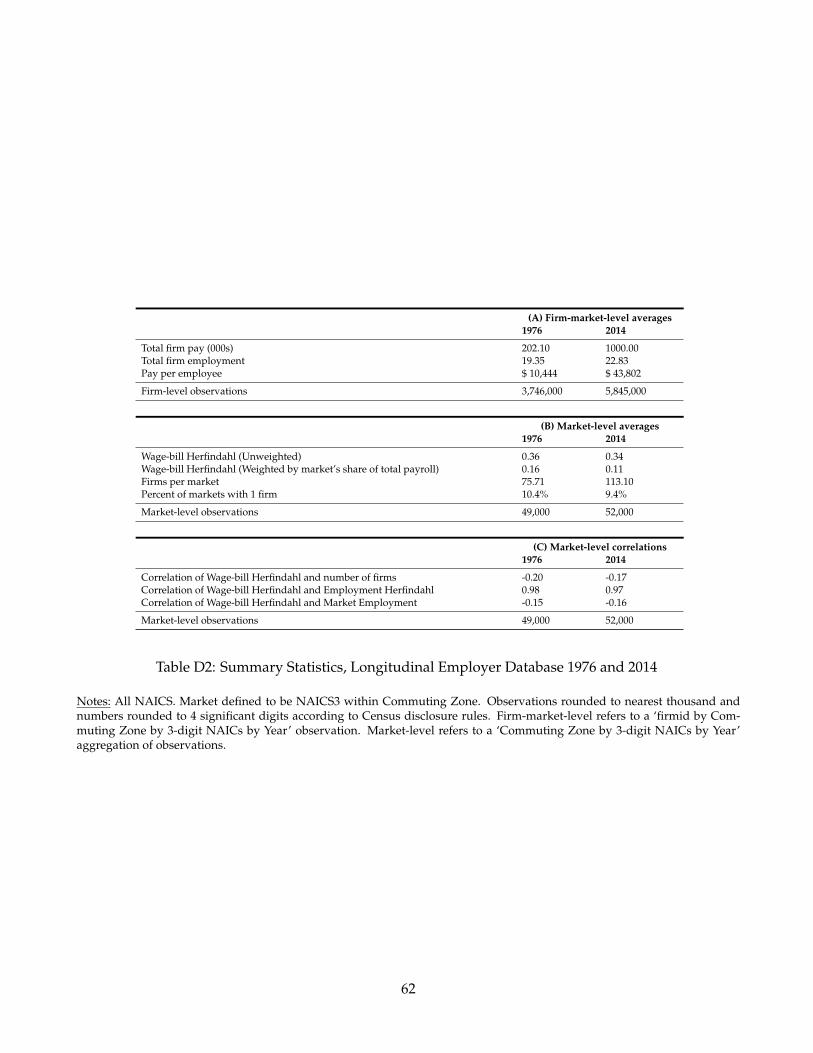
(A) Firm-market-level averages1976 2014

Total firm pay (000s) 202.10 1000.00Total firm employment 19.35 22.83Pay per employee $ 10,444 $ 43,802

Firm-level observations 3,746,000 5,845,000

(B) Market-level averages1976 2014

Wage-bill Herfindahl (Unweighted) 0.36 0.34Wage-bill Herfindahl (Weighted by market’s share of total payroll) 0.16 0.11Firms per market 75.71 113.10Percent of markets with 1 firm 10.4% 9.4%

Market-level observations 49,000 52,000

(C) Market-level correlations1976 2014

Correlation of Wage-bill Herfindahl and number of firms -0.20 -0.17Correlation of Wage-bill Herfindahl and Employment Herfindahl 0.98 0.97Correlation of Wage-bill Herfindahl and Market Employment -0.15 -0.16

Market-level observations 49,000 52,000

Table D2: Summary Statistics, Longitudinal Employer Database 1976 and 2014

Notes: All NAICS. Market defined to be NAICS3 within Commuting Zone. Observations rounded to nearest thousand andnumbers rounded to 4 significant digits according to Census disclosure rules. Firm-market-level refers to a ‘firmid by Com-muting Zone by 3-digit NAICs by Year’ observation. Market-level refers to a ‘Commuting Zone by 3-digit NAICs by Year’aggregation of observations.

62

E Mathematical derivations

This section provides detailed derivations of mathematical formulae that appear in the main text. It covers: (i) the householdproblem (Section E.1) (ii) the firm problem (Section E.2), (iii) market equilibrium (Proposition 1.1) (Section E.3), (iv) generalequilibrium and aggregation (Proposition 1.2) (Section E.4), (v) relationship between the labor share and concentration (Propo-sition 1.3) (Section E.5), (vi) closed form general equilibrium solution and scaling properties used in calibration (Section E.6),(vii) reduced form and structural labor supply elasticities (Section E.7), (viii) pass-through expression (Section E.8), (ix) expres-sions used in the discussion of corporate taxes (Section E.9), (x) proofs of merger results (Proposition 3) (Section E.10).

E.1 Household problem - Section 1.2

• The household’s problem is

maxnijt ,cijt ,Kt+1

∞

∑t=0

βtU (Ct, N t)

where

N t =

[ˆn

θ+1θ

jt dj] θ

θ+1

njt =

∑i∈j

nη+1

η

ijt

η

η+1

Ct =

ˆ∑i∈j

cijtdj

subject to the initial endowment K0 > 0, and the following budget constraint in each period, in which it takes all pricesas given, these include the wage wijt at all firms-ij, rental rate Rt and profits Πt as given:

Ct + Kt+1 − (1− δ)Kt =

ˆ∑i∈j

wijtnijtdj + RtKt + Πt

E.1.1 First order conditions

• The first order conditions for consumption and capital give

UC (Ct, N t) = βUC (Ct+1, N t+1) [Rt+1 + (1− δ)]

• The first order conditions for consumption and labor supply to firm-ij gives

wijt =∂njt

∂nijt

∂N t∂njt

(−UN (Ct, N t)

UC (Ct, N t)

)

E.1.2 Deriving supply system

• Define the following terms. The market wage wjt is the number that satisfies wjtnjt = ∑i∈j wijtnijt. The aggregate wage W t

is the number that satisfies W t N t =´

wjtnjtdj.

• We can write the first order condition as:

wijtnijt =

(∂njt

∂nijt

nijt

njt

)(∂N t∂njt

njt

N t

)(−UN (Ct, N t)

UC (Ct, N t)

)N t

63

• Using the labor disutility indexes, note that

∂njt

∂nijt

nijt

njt=

(nijt

njt

) η+1η

, therefore, ∑i∈j

∂njt

∂nijt

nijt

njt= 1

∂N t∂njt

njt

N t=

( njt

N t

) θ+1θ

, therefore,ˆ

∂N t∂njt

njt

N tdj = 1

• Using these results and aggregating the first order condition over i ∈ j, then over j ∈ [0, 1]

Aggregate over i ∈ j : wjtnjt =

(∂N t∂njt

njt

N t

)(−UN (Ct, N t)

UC (Ct, N t)

)N t

Aggregate over j ∈ [0, 1] : W t N t = −UN (Ct, N t)

UC (Ct, N t)N t

W t = −UN (Ct, N t)

UC (Ct, N t)

• Aggregating the first order condition over markets j ∈ [0, 1], and then substituting the aggregate inverse labor supplycurve back into the first order condition we can obtain the market supply curve:

wjtnjt =

(∂N t∂njt

njt

N t

)(−UN (Ct, N t)

UC (Ct, N t)

)N t

wjtnjt =

( njt

N t

) θ+1θ

W t N t

njt =

(wjt

W t

)θ

N t

which also implies that∂N t∂njt

njt

N t=

wjtnjt

W t N t.

• Substituting this into the first order condition we can obtain the firm supply curve:

wijtnijt =

(∂njt

∂nijt

nijt

njt

)(∂N t∂njt

njt

N t

)(−UN (Ct, N t)

UC (Ct, N t)

)N t

wijtnijt =

(nijt

njt

) η+1η (wjtnjt

W t N t

)W t N t

nijt =

(wijt

wjt

)η (wjt

W t

)θ

N t

• We can now compute expressions for the wage indexes wjt and W t.

64

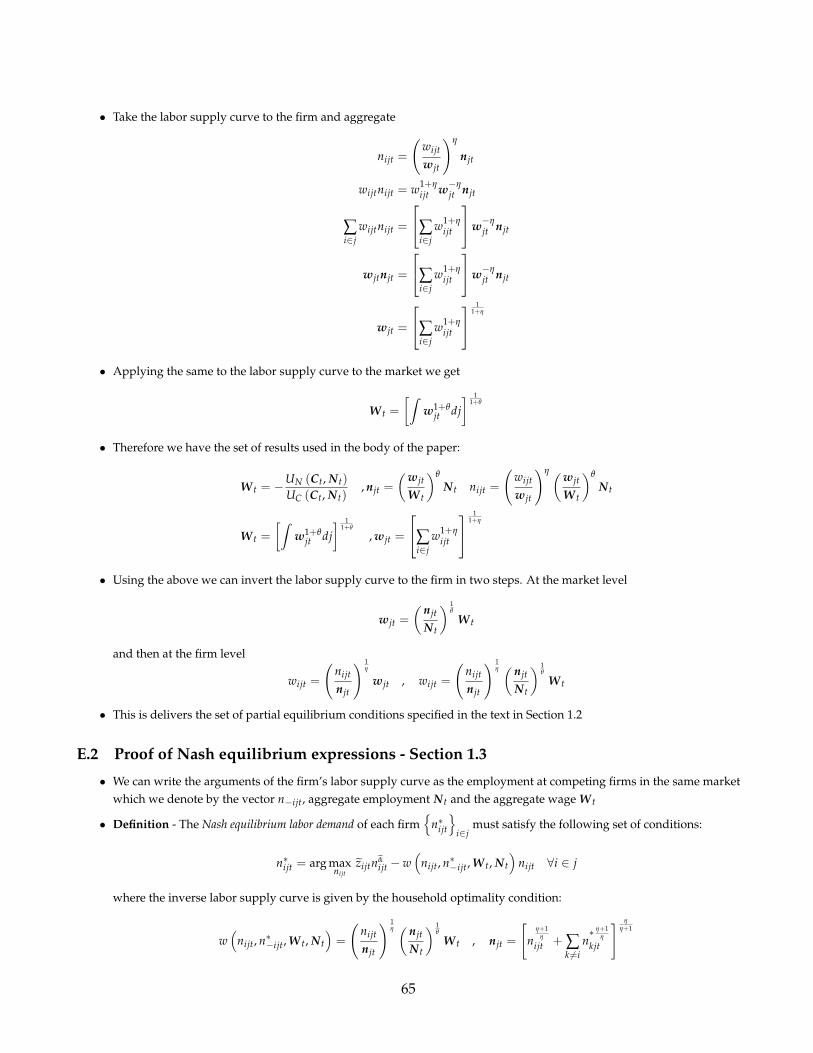
• Take the labor supply curve to the firm and aggregate

nijt =

(wijt

wjt

)η

njt

wijtnijt = w1+ηijt w−η

jt njt

∑i∈j

wijtnijt =

∑i∈j

w1+ηijt

w−ηjt njt

wjtnjt =

∑i∈j

w1+ηijt

w−ηjt njt

wjt =

∑i∈j

w1+ηijt

11+η

• Applying the same to the labor supply curve to the market we get

W t =

[ˆw1+θ

jt dj] 1

1+θ

• Therefore we have the set of results used in the body of the paper:

W t = −UN (Ct, N t)

UC (Ct, N t), njt =

(wjt

W t

)θ

N t nijt =

(wijt

wjt

)η (wjt

W t

)θ

N t

W t =

[ˆw1+θ

jt dj] 1

1+θ

, wjt =

∑i∈j

w1+ηijt

11+η

• Using the above we can invert the labor supply curve to the firm in two steps. At the market level

wjt =

( njt

N t

) 1θ

W t

and then at the firm level

wijt =

(nijt

njt

) 1η

wjt , wijt =

(nijt

njt

) 1η ( njt

N t

) 1θ

W t

• This is delivers the set of partial equilibrium conditions specified in the text in Section 1.2

E.2 Proof of Nash equilibrium expressions - Section 1.3

• We can write the arguments of the firm’s labor supply curve as the employment at competing firms in the same marketwhich we denote by the vector n−ijt, aggregate employment N t and the aggregate wage W t

• Definition - The Nash equilibrium labor demand of each firm

n∗ijt

i∈jmust satisfy the following set of conditions:

n∗ijt = arg maxnijt

zijtnαijt − w

(nijt, n∗−ijt, W t, N t

)nijt ∀i ∈ j

where the inverse labor supply curve is given by the household optimality condition:

w(

nijt, n∗−ijt, W t, N t

)=

(nijt

njt

) 1η ( njt

N t

) 1θ

W t , njt =

[n

η+1η

ijt + ∑k 6=i

n∗ η+1

η

kjt

] ηη+1

65

• The first order condition for each firm is as follows, where we write the marginal revenue product of labor mrplijt =

αzijtnα−1ijt :

mrplijt =∂w(

nijt, n∗−ijt, W t, N t

)∂nijt

nijt + w(

nijt, n∗−ijt, W t, N t

)

mrplijt = w(

nijt, n∗−ijt, W t, N t

) ∂w(

nijt, n∗−ijt, W t, N t

)∂nijt

nijt

w(

nijt, n∗−ijt, W t, N t

) + 1

• The elasticity is

∂ log w(

nijt, n∗−ijt, W t, N t

)∂ log nijt

=1η+

(1θ− 1

η

) ∂ log njt

(nijt, n∗−ijt

)∂ log nijt

∂ log w(

nijt, n∗−ijt, W t, N t

)∂ log nijt

=1η+

(1θ− 1

η

)(nijt

njt

) η+1η

• We can write this in terms of the payroll share of the firm. Using our expression for the labor supply curve to the firm

sijt =wijtnijt

∑i∈j wijtnijt=

(nijtnjt

) 1η(

njtN t

) 1θ nijt

∑i∈j

(nijtnjt

) 1η(

njtN t

) 1θ nijt

=n

η+1η

ijt

∑i∈j nη+1

η

ijt

=

(nijt

njt

) η+1η

.

• This gives

∂ log w(

nijt, n∗−ijt, W t, N t

)∂ log nijt

= sijt1θ+(

1− sijt

) 1η

• Define the equilibrium inverse labor supply elasticity ε∗ijt as

ε∗ijt =

[sijt

1θ+(

1− sijt

) 1η

]−1

• Then we can write the wage as

w∗ijt = µ∗ijtmrplijt

µ∗ijt =1

sijt1θ +

(1− sijt

)1η + 1

µ∗ijt =

[sijt

1θ +

(1− sijt

)1η sijt

]−1

[sijt

1θ +

(1− sijt

)1η

]−1+ 1

µ∗ijt =ε∗ijt

ε∗ijt + 1

• This is delivers the set of partial equilibrium conditions specified in the text in Section 1.3

w∗ijt = µ∗ijtmrplijt

µ∗ijt =εijt

εijt + 1

ε∗ijt =

[sijt

1θ+(

1− sijt

) 1η

]−1

66

E.3 Proof of Proposition 1.1

• Collect terms in the labor supply curve that are common to all firms in the market, xj := wθ−ηj W−θ N.

• We have the following conditions

mrplij = αzijnα−1ij

nij = wηij × xj

wij = µ(

sij

)mrplij

• Substituting the labor supply curve into the mrplij definition, and then the pricing condition into the labor supply curvefor wij we have

mrplij =[

αzijµ(

sij

)−η(1−α)xα−1

j

]×mrpl−η(1−α)

ij

mrplij =[

αzijµ(

sij

)−η(1−α)xα−1

j

] 11+η(1−α)

• Substiting this back into the optmiality condition:

wij =[µ(

sij

)αzij

] 11+η(1−α) × x

− 1−α1+η(1−α)

j =[µ(

sij

)zij

] 11+η(1−α) × g

(xj

)• The definition of the payroll share, combined with the labor supply curve gives

sij =wijnij

∑k∈j wkjnkj=

wij

(wijwj

)η (wjW

)θN

∑k∈j wkj

(wkjwj

)η (wjW

)θN

=wη+1

ij

∑k∈j wη+1kj

=wη+1

ij

∑k∈j wη+1kj

.

• Under the above expression for wij:

sij =

[µ(

sij

)zij

] η+11+η(1−α)

∑k∈j

[µ(

skj

)zkj

] η+11+η(1−α)

.

• Now recall that zij is the firm productivity under the firm’s optimal capital decision, and αis the corresponding exponent:

yi = zi

(k∗ (ni, zi, R)1−γ nγ

i

)α= zinα

i

zi = [1− (1− γ) α] z1

1−(1−γ)α

i

((1− γ) α

R

) (1−γ)α1−(1−γ)α

α =γα

1− (1− γ) α

• Substituting these in

sij =

[µ(

sij

)1−(1−γ)αzij

] η+11−(1−γ)α+η(1−α)

∑k∈j

[µ(

skj

)1−(1−γ)αzkj

] η+11−(1−γ)α+η(1−α)

• This is the expression in Proposition 1.1, which holds for all firms i in market j, and is independent of aggregates.

67

• Note that in the limit as γ→ 1, then we can check that we obtain the no-capital expression from above

sij =

[µ(

sij

)zij

] η+11+η(1−α)

∑k∈j

[µ(

skj

)zkj

] η+11+η(1−α)

• Additionally in the limit with α→ 1, we have

sij =

[µ(

sij

)zij

]η+1

∑k∈j

[µ(

skj

)zkj

]η+1

• In the limit α→ 1 with γ < 1:

sij =

[µ(

sij

)γzij

] η+1η+γ

∑k∈j

[µ(

skj

)γzkj

] η+1η+γ

E.4 Proof of Proposition 1.2

• We proceed in three steps.

• First, consider an economy with a single nest, with a single elasticity of substitution η, and consider the case of labor asthe only input into production with decreasing returns α ∈ (0, 1].

• Our starting point is the following set of equations, where we can take the markdown as exogenous. These describe firmlevel (i) output, (ii) labor supply, (iii) labor demand optimality, (iv) marginal revenue product:

yi = zinαi

ni =(wi

w

)ηn

wi = µimrpli

mrpli = αzinα−1i

• We then have two aggregation conditions: (i) output, (ii) wage index

y =

ˆyidi

w =

[ˆw1+η

i di] 1

1+η

• This set of 6 equations are our inputs to the following claim.

• Claim - The aggregates y, w, n can be written:

y = ωznα

w = µαznα−1

68

where

z =

[ˆz

1+η1+η(1−α)

i di] 1+η(1−α)

1+η

µ =

[ˆ ( ziz

) 1+η1+η(1−α)

µ1+η

1+η(1−α)

i di

] 1+η(1−α)1+η

ω =

ˆ ( ziz

) 1+η1+η(1−α)

(µiµ

) ηα1+η(1−α)

di

• Proof

• With decreasing returns to scale, we first solve out for the marginal revenue product of labor. Note that here we onlymultiply and divide by z:

mrpli = αzinα−1i

mrpli = αzi

((wiw

)ηn)α−1

mrpli =( zi

z

)wη(α−1)

i

⟨αznα−1

⟩wη(1−α)

mrpli =( zi

z

)µ

η(α−1)i mrplη(α−1)

i

⟨αznα−1

⟩wη(1−α)

mrpli =( zi

z

) 11+η(1−α)

µ− η(1−α)

1+η(1−α)

i

⟨αznα−1

⟩ 11+η(1−α) w

η(1−α)1+η(1−α)

• We can check that in the case of α = 1, then mrpli = zi.

• Using this in the wage

wi = µimrpli

wi =( zi

z

) 11+η(1−α)

µ1

1+η(1−α)

i

⟨αznα−1

⟩ 11+η(1−α) w

η(1−α)1+η(1−α)

• Now aggregating:

w =

[ˆw1+η

i di] 1

1+η

w =

[ˆ ( ziz

) 1+η1+η(1−α)

µ1+η

1+η(1−α)

i di

] 11+η ⟨

αznα−1⟩ 1

1+η(1−α) wη(1−α)

1+η(1−α)

w1

1+η(1−α) =

[ˆ ( ziz

) 1+η1+η(1−α)

µ1+η

1+η(1−α)

i di

] 11+η ⟨

αznα−1⟩ 1

1+η(1−α)

w =

[ˆ ( ziz

) 1+η1+η(1−α)

µ1+η

1+η(1−α)

i di

] 1+η(1−α)1+η

×⟨

αznα−1⟩

w = µ⟨

αznα−1⟩

• This delivers the first result. Note that if α = 1, then

µ =

[ˆ ( ziz

)1+ηµ

1+ηi di

] 11+η

69

• Now turning to firm output, under the labor supply curve and labor demand:

yi = zinαi

yi = zi

((wiw

)ηn)α

yi = zi

((µimrpli

w

)η

n)α

yi = ziµαηi mrplαη

i

(1w

)αη

nα

• Using the previous expression for mrpli:

yi = ziµαηi

( ziz

) 11+η(1−α)

µ− η(1−α)

1+η(1−α)

i

⟨αznα−1

⟩ 11+η(1−α) w

η(1−α)1+η(1−α)

αη (1w

)αη

nα

yi = z

[( ziz

)1+ αη1+η(1−α)

µαη(

1− η(1−α)1+η(1−α)

)i

⟨αznα−1

⟩wη(1−α)

αη1+η(1−α)

(1w

)αη]

nα

yi = z

[( ziz

) 1+η1+η(1−α)

µαη

1+η(1−α)

i

⟨αznα−1

⟩wη(1−α)

αη1+η(1−α)

(1w

)αη]

nα

Given that we have shown that w = µαznα−1, we can use this to simplify ·:

yi = z( zi

z

) 1+η1+η(1−α)

µαη

1+η(1−α)

i

(wµ

)wη(1−α)

αη1+η(1−α)

(1w

)αη

nα

yi = z

[( ziz

) 1+η1+η(1−α)

(µiµ

) αη1+η(1−α)

]nα

• Then aggregating:

y =

ˆyidi

y =

[ˆ ( ziz

) 1+η1+η(1−α)

(µiµ

) αη1+η(1−α)

di

]× 〈znα〉

y = ω× znα

• This delivers the second result. Note that if α = 1, then

ω =

ˆ ( ziz

)1+η(

µiµ

)η

di

• We stil need to show that the productivity term z is correct. Notice that up to this point these derivations would holdunder any z. We pin down z, by requiring that if there are no distortions (µi = 1 for all firms), then the aggregatemarkdown is also µ = 1. This requires:

1 =

[ˆ ( ziz

)1+ηdi] 1

1+η

z =

[ˆz

1+η1+η(1−α)

i di] 1+η(1−α)

1+η

which also implies that in an undistorted economy, since ω = 1, then output is simply y = znα.

70

• This also implies that in the expression for µ and the expression for ω, the productivity terms are well-defined weights:

µ =

[ˆ ( ziz

) 1+η1+η(1−α)

µ1+η

1+η(1−α)

i di

] 1+η(1−α)1+η

,ˆ ( zi

z

) 1+η1+η(1−α) di = 1

ω =

ˆ ( ziz

) 1+η1+η(1−α)

(µiµ

) αη1+η(1−α)

di ,ˆ ( zi

z

) 1+η1+η(1−α) di = 1

• Using the above results we can now turn to the nested economy.

• Inner nest

– We take the same approach as above, starting with the isomorphic 6 conditions at the firm level and now thoseexpressing market level aggregates:

– Firm conditions: We have 4 conditions representing firm output, labor supply, labor demand, and the marginalrevenue product of labor:

yij = zijnαij

nij =

(wij

wj

)η

nj

wij = µijmrplij

mrplij = αzijnα−1ij

– Market aggregates: We then have two aggregation conditions: (i) market output, (ii) market wage index

yj = ∑i∈j

yij

wj =

∑i∈j

w1+ηij

11+η

– Following the same steps as above, it is clear that we can show that:

– Claim - The market aggregates

yj, wj, nj

can be written:

yj = ωjzjnαj

wj = µjαzjnα−1j

where

zj =

∑i∈j

z1+η

1+η(1−α)

ij

1+η(1−α)

1+η

µj =

∑i∈j

(zij

zj

) 1+η1+η(1−α)

µ1+η

1+η(1−α)

ij

1+η(1−α)

1+η

ωj = ∑i∈j

(zizj

) 1+η1+η(1−α) (µi

µ

) ηα1+η(1−α)

• Outer nest

– The solution to the inner nests allows us to establish a similar set of 6 conditions

71

– Market level: We have 3 conditions representing market output, aggregate labor supply, market labor demand:

yj = ωjzjnαj

nj =

(wj

W

)θ

N

wj = µjαzjnα−1j

– Economy aggregates: We have two aggregation conditions: (i) aggregate output, (ii) aggregate wage index

Y =

ˆyjdj

W =

[ˆw1+θ

j dj] 1

1+θ

• Following the above steps again, we can obtain:

Y = ΩZNα

W = µαZNα−1

where

Z =

[ˆz

1+θ1+θ(1−α)

j

] 1+θ(1−α)1+θ

µ =

[ˆ ( zj

Z

) 1+θ1+θ(1−α)

µ1+θ

1+θ(1−α)

j dj

] 1+θ(1−α)1+θ

Ω =

ˆ ( zj

Z

) 1+η1+η(1−α)

(µj

µ

) ηα1+η(1−α)

ωjdj

• This delivers the main expressions in Proposition 1.2, in the case of an economy without capital and decreasing returnsto labor.

E.4.1 Adding capital

• The value-added production function of the firm in our model is

yi = zi

(k1−γ

i nγi

)α

• The optimal choice of capital solves

k∗i (zi, ni, R) = arg maxki

zi

(k1−γ

i nγi

)α− Rki

k∗i (zi, ni, R) =((1− γ) αzi

R

) 11−(1−γ)α

nγα

1−(1−γ)α

i

• We can substitute this back into output to obtain:

yi = z1

1−(1−γ)α

i

((1− γ) α

R

) (1−γ)α1−(1−γ)α

nγα

1−(1−γ)α

i

72

• Note that in terms of factor payment shares, capital is competitively priced:

Rki = α (1− γ) yi

• Combining these, profits are

πi = yi − Rki − wini

πi = [1− α (1− γ)] yi − wini

πi = [1− α (1− γ)] z1

1−(1−γ)α

i

((1− γ) α

R

) (1−γ)α1−(1−γ)α

nγα

1−(1−γ)α

i − wini

• We can write this as

πi = yi − wini

yi = zinαi

zi = [1− α (1− γ)] z1

1−(1−γ)α

i

((1− γ) α

R

) (1−γ)α1−(1−γ)α

α =γα

1− (1− γ) α

• Note that this implies that

yi = yi − Rki = [1− γ (1− α)] yi

yi =

[1

1− γ (1− α)

]yi

• It should therefore be clear that what we have obtained so far in our aggregation results implies the following:

1. Market level - At the market level, define yj = ∑i∈j yij, then

yj = ωj zjnαj

wj = µj zjαnα−1j

where

ωj, µj

are as before, except with α in place of α, and we define zj as:

zj =

∑i∈j

z1+η

1+η(1−α)

ij

1+η(1−α)

1+η

µj =

∑i∈j

(zij

zj

) 1+η1+η(1−α)

µ1+η

1+η(1−α)

ij

1+η(1−α)

1+η

ωj = ∑i∈j

(zij

zj

) 1+η1+η(1−α) (µi

µ

) ηα1+η(1−α)

2. Aggregate level - At the aggregate level, define Y =´

yjdj, then

Y = ΩZN α

W = µαZN α−1

73

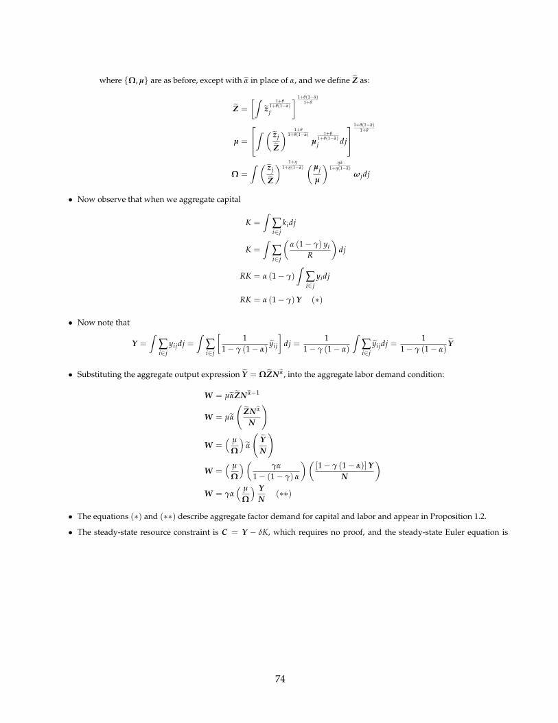
where Ω, µ are as before, except with α in place of α, and we define Z as:

Z =

[ˆz

1+θ1+θ(1−α)

j

] 1+θ(1−α)1+θ

µ =

ˆ ( zj

Z

) 1+θ1+θ(1−α)

µ1+θ

1+θ(1−α)

j dj

1+θ(1−α)

1+θ

Ω =

ˆ ( zj

Z

) 1+η1+η(1−α)

(µj

µ

) ηα1+η(1−α)

ωjdj

• Now observe that when we aggregate capital

K =

ˆ∑i∈j

kidj

K =

ˆ∑i∈j

(α (1− γ) yi

R

)dj

RK = α (1− γ)

ˆ∑i∈j

yidj

RK = α (1− γ)Y (∗)

• Now note that

Y =

ˆ∑i∈j

yijdj =ˆ

∑i∈j

[1

1− γ (1− α)yij

]dj =

11− γ (1− α)

ˆ∑i∈j

yijdj =1

1− γ (1− α)Y

• Substituting the aggregate output expression Y = ΩZN α, into the aggregate labor demand condition:

W = µαZN α−1

W = µα

(ZN α

N

)

W =( µ

Ω

)α

(YN

)

W =( µ

Ω

)( γα

1− (1− γ) α

)([1− γ (1− α)]Y

N

)W = γα

( µ

Ω

) YN

(∗∗)

• The equations (∗) and (∗∗) describe aggregate factor demand for capital and labor and appear in Proposition 1.2.

• The steady-state resource constraint is C = Y − δK, which requires no proof, and the steady-state Euler equation is

74

1 = β [R + (1− δ)], these can be combined with optimal capital demand to yield:

C = Y − δK

C = Y − δ

RRK

C =

[1− δ

R(1− γ) α

]Y

C =

[1− δ

R(1− γ) α

]Y

1− γ (1− α)

C =

[1− βδ

1− β (1− δ)(1− γ) α

]Y

1− γ (1− α)

where we denote the constant sC, which is the consumption share of output. These expressions appear in the main text.

• This implies that given µ, and Ω, we can solve for equilibrium

Y , W , N, C

from

W = µαZN α−1

W =UN (C, N)

UC (C, N)

C = sCY

1− γ (1− α)

Y = ΩZN α

• In the case of UN/UC = N ϕC−σ, as is the case under GHH (σ = 0) or CRRA preferences (σ ≥ 1), then all aggregatescan be solved in closed form using the following equations from top to bottom:

N =

[(sC

1− γ (1− α)Ω

)−σϕ

(αµ)ϕ Z(1−σ)ϕ

] 11+ϕ(1−α)+σϕα

W = µαZN α−1

Y = ΩZN α

C =sc

1− γ (1− α)Y

Y =1

1− (1− γ) αY

R =1β− (1− δ)

K =(1− γ) α

RY

• Note that in the case of no wealth-effects on labor supply σ = 0, and we have the result, cited in the text, that theequilibrium aggregate employment and wage are independent of Ω,

N =[αµZ

] ϕ1+ϕ(1−α) , W = µαZN α−1

E.4.2 Production function

• In the main tet of the paper we provide the above conditions, but instead with the output as follows, which we nowderive.

Y = Ω1−(1−γ)αZ(

K1−γ Nγ)α

where we also need to specify Z.

75

• First we need to go remove the optimal capital decisions encoded in zij and consequently zj and Z.

• Recall that

zij = (1− (1− γ) α) z1

1−(1−γ)α

ij

((1− γ) α

R

) (1−γ)α1−(1−γ)α

, zj =

∑i∈j

z1+η

1+η(1−α)

ij

1+η(1−α)

1+η

, Z =

[ˆz

1+θ1+θ(1−α)

j dj] 1+θ(1−α)

1+θ

• Substituting zij into zj, we can define market productivity as follows, which gives the following implication:

zj :=

∑i∈j

z1+η

1−(1−γ)α+η(1−α)

ij

1−(1−γ)α+η(1−α)

1+η

=⇒ zj = (1− (1− γ) α) z1

1−(1−γ)α

j

((1− γ) α

R

) (1−γ)α1−(1−γ)α

• We can do the same for market and aggregate productivity:

Z :=[ˆ

z1+θ

1−(1−γ)α+θ(1−α)

j dj] 1−(1−γ)α+θ(1−α)

1+θ

=⇒ Z = (1− (1− γ) α) Z1

1−(1−γ)α

((1− γ) α

R

) (1−γ)α1−(1−γ)α

• Note that this implies that the relationship between Z and Z given in the text

Z =

[R

(1− γ) α

](1−γ)α[

Z1− (1− γ) α

]1−(1−γ)α

• Now return to the aggregate production function Y = ΩZN α and substitute in (i) the definitions of α, (ii) Z, and, (iii)Y = [1− (1− γ) α]Y , (iv) the aggregate capital demand condition R = (1− γ) α (Y/K), thsi gives the expression inProposition 1.2:

Y = ΩZNγα

1−(1−γ)α

Y = Ω (1− (1− γ) α) Z1

1−(1−γ)α

((1− γ) α

R

) (1−γ)α1−(1−γ)α

Nγα

1−(1−γ)α

Y = ΩZ1

1−(1−γ)α

(KY

) (1−γ)α1−(1−γ)α

Nγα

1−(1−γ)α

Y = Ω1−(1−γ)αZ(

K1−γ Nγ)α

where we have the productivity terms which are described in the footnote of Proposition 1.2:

zj =

∑i∈j

z1+η

1−(1−γ)α+η(1−α)

ij

1−(1−γ)α+η(1−α)

1+η

, Z =

[ˆz

1+θ1−(1−γ)α+θ(1−α)

j dj] 1−(1−γ)α+θ(1−α)

1+θ

E.5 Proof of Proposition 1.3 - Labor share and concentration

• Rearranging the above conditions immediately gives the labor share

LS :=

´∑i∈j wijnijdj´

∑i∈j yijdj=

W NY

= γα( µ

Ω

)• Since µ and Ω are independent of the supply block of the model, then they are independent of aggregates and prefer-

ences, and so is the labor share. That is, we only have to solve market equilibria to compute the labor share.

• We now show that the expression linking the labor share and aggregate HHIwn holds.

76

• We can use ‘tilde’ objects and then scale up at the end:

lsij =wijnij

yij=

wijnij

zijnαij

= αwij

αzijnα−1ij

= αwij

mrplij= αµij

• Therefore the inverse of the labor share is:ls−1ij =

1α

µ−1ij

• Note that from our earlier expression for the markdown:

µ−1ij = sijt

(1θ− 1

η

)+

1η+ 1 =

η + 1η

+ sijt

(θ + 1

θ− η + 1

η

)• Now the market inverse labor share is

ls−1ij =

∑i∈j yij

∑i∈j wijnij= ∑

i∈j

wijnij

∑i∈j wijnij

yij

wijnij= ∑

i∈jsij ls

−1ij

which using the above, gives:

ls−1ij =

1α

[(1− hhij

) η + 1η

+ hhijθ + 1

θ

]where hhij = ∑i∈j s2

ij.

• Then the aggregate labor share is as follows, where we use our definiton HHI =´

sjhhijdj:

LS =

[ ´∑i∈j yijdj´

∑i∈j wijnijdj

]−1

=

[ˆsj ls−1j dj

]−1

LS = α

[HHI

(θ

θ + 1

)−1+ (1− HHI)

(η

η + 1

)−1]−1

• Now note thatY =

11− (1− γ) α

Y

thereforeLS =

W NY

=W N

11−(1−γ)α

Y= [1− (1− γ) α] LS,

so under α = αγ/ (1− (1− γ) α) we have

LS = αγ

[HHI

(θ

θ + 1

)−1+ (1− HHI)

(η

η + 1

)−1]−1

• This is the expression in Proposition 1.3.

• This also established the following claims: (i) the moments LS and HHI are independent of aggregate preferences andshifters in labor supply and productivity which we study below A and ϕ, since the capital share is KS = α (1− γ),then this is also independent of preferences, therefore (ii) we can estimate the model without specifying aggregatepreferences.

77

E.6 Scaling the economy

• Here we prove our claim in the text that we can choose scaling parameters for productivity and labor supply that canalways be chosen to match average firm size and average worker pay without affecting any of the other moments of theeconomy.

• Suppose we add two constants to the above economy A and ϕ such that the firm production function after optimizingout capital and the aggregate labor supply curve are:

yij = Azijnαij

W = −UN (C, N)

UC (C, N)= ϕ−1/ϕ N1/ϕCσ

• We claim that we can always choose these constants to match two moments of the data: average firm size, and averageworker pay.

• Note that the above labor supply curve obtains under either CRRA or GHH preferences, where GHH preferences arethe case of σ = 0:

U(C, N) =C1−σ

1− σ− ϕ−1/ϕ N1+ 1

ϕ

1 + 1ϕ

, U (C, N) = u

(C− ϕ−1/ϕ N1+ 1

ϕ

1 + 1ϕ

)

• Note that this implies that the changes to the set of equilibrium conditions are that aggregate output, labor demand andlabor supply are:

Y = ΩAZN α

W = µαAZN α−1

N = ϕW ϕC−σϕ

• Combined these imply the same expression for the labor share:

W N =( µ

Ω

)αY

which gives

Y =W N( µΩ

)α

• Consider the following two moments: (i) Average firm size (AveFirmSize), (ii) Average worker pay (AveWorkerPay)

• The average firm size in the economy is

AveFirmSize :=

´∑i∈j nijdj´

Mjdj=

´∑i∈j

(wijwj

)η (wjW

)θNdj´

Mjdj

• Define the following:

νij :=

(wij

wj

)η (wj

W

)θ

• Using this

AveFirmSize =

´∑i∈j νijdj´

MjdjN

• Denote ν =´

∑i∈j νijdj .

78

• The average worker pay in the economy is

AveWorkerPay =

´∑i∈j wijnijdj´

∑i∈j nijdj

=W N

AveFirmSize×´

Mjdj

AveWorkerPay =Wν

• We can re-write these:

N = AveFirmSize×´

Mjdjν

W = AveWorkerPay× ν

• Claim - The aggregate ν is independent of all other aggregates including the shifters A and ϕ

– Using our above results, but now including the shifter terms:(wij

wj

)=

µijαzij Anα−1ij

µjαzj Anα−1j(

wij

wj

)=

(µij zij

µj zj

) 11+η(1−α)

and using a similar approach at the market level:

(wj

W

)=

(µj zj

µZ

) 11+θ(1−α)

– Therefore we have the following equation which implies that νij is independent of aggregates including the shiftparameters A and ϕ

νij =

(µij zij

µj zj

) 11+η(1−α)

(µj zj

µZ

) 11+θ(1−α)

• We can then write the following system of equations, which we describe below

N = AveFirmSize×´

Mjdjν

W = AveWorkerPay× ν

Y =W N( µΩ

)α

Y =Y

1− (1− γ) α

K =(1− γ) αY

RC = Y − δK

• Starting with a solution of the market equilibria, we can obtain ν, Ω, µ which we have proven are independent ofaggregates and shifters

A, ϕ

. Then given data on AveFirmSizeData and AveWorkerPayData , we can put data into

the first two expressions above, and use these to compute N and W . Given these we can use the remaining equationsto compute all other aggregate quantities Y , C, K. What remains is to choose A and ϕ to be consistent with these

79

aggregates. For this we use the two conditions that have not been used above by themselves: output and labor supply

Y = ΩAZN α , N = ϕW ϕC−σϕ,

which imply that

A =Y

ΩZN α, ϕ =

NW ϕC−σϕ .

• Proceeding in this way we can always choose shifters A and ϕ in order to match data on average firm size and averageworker pay.

• Once these are pinned down, then the system of equilibrium conditions without the moment conditions can be solved.Going from top to bottom, the equilibrium is computed:

N =

[ϕ

(sc

1− γ (1− α)Ω

)−σϕ

(αµ)ϕ(

AZ)(1−σ)ϕ

] 11+ϕ(1−α)+σϕα

W = µαAZN α−1

Y = ΩAZN α

C =sc

1− γ (1− α)Y

Y =1

1− (1− γ) αY

R =1β− (1− δ)

K =(1− γ) α

RY

E.7 Reduced form labor supply elasticities

• We derive the expression linking reduced form and structural labor supply elasticities in Section 2.1

• Conisder the labor supply curve to the firm

nijt =

(wijt

wjt

)η (wjt

W t

)θ

N t

• Consider a first order approximation around the Nash equilibrium following any change to firms in the market

∆ log nijt = η∆ log wijt + (θ − η) ∑k∈j

∂ log wjt

∂ log wkjt

∣∣∣∣∣n∗−kjt

∆ log wkjt

∆ log nijt = η∆ log wijt + (θ − η) ∑k∈j

∂ log wjt

∂ log wkjt

∣∣∣∣∣n∗−kjt

∆ log wkjt

• Consider the labor supply curve to the firm

wijt =

(nijt

njt

) 1η ( njt

N t

) 1θ

W t

log wijt =1η

log nijt +

(1θ− 1

η

)log njt + Aggregates

• Consider a first order approximation around the Nash equilibrium, denoted by asterisks, following any change to firms

80

in the market

∆ log wijt =1η

∆ log nijt +

(1θ− 1

η

)∑k∈j

∂ log njt

∂ log nkjt

∣∣∣∣∣n∗−kjt

∆ log nkjt

∆ log wijt =

1η+

(1θ− 1

η

)∂ log njt

∂ log nijt

∣∣∣∣∣n∗ijt

∆ log nijt +

(1θ− 1

η

)∑k 6=i

∂ log njt

∂ log nkjt

∣∣∣∣∣n∗−kjt

∆ log nkjt

∆ log wijt =

(1η+

(1θ− 1

η

)s∗ijt

)∆ log nijt +

(η − θ

θη

)∑k 6=i

s∗kjt∆ log nkjt

• The definition of the reduced form labor supply elasticity in the text is

εijt =∆ log nijt

∆ log wijt

• Using the above approximation:

εijt =∆ log nijt(

1η +

(1θ −

1η

)s∗ijt)

∆ log nijt +(

η−θθη

)∑k 6=i s∗kjt∆ log nkjt

εijt =1(

1η +

(1θ −

1η

)s∗ijt)+(

η−θθη

) ∑k 6=i s∗kjt

∆ log nkjt∆ log nijt

εijt =

(1η +

(1θ −

1η

)s∗ijt)−1

1 +(

1η +

(1θ −

1η

)s∗ijt)−1 ( η−θ

θη

) ∑k 6=i s∗kjt

∆ log nkjt∆ log nijt

εijt =

⟨1

1 + ε∗ijt

(η−θθη

) ∑k 6=i s∗kjt

∆ log nkjt∆ log nijt

⟩ ε∗ijt

• This gives the expression in the text.

E.8 Pass-through expression

• We derive the pass-through expression that appears in Section 3.1

• Consider a firm’s Nash equilibrium wagew∗ijt = µ∗ijtmrplijt

• Here we have

mrplijt = αzijtnα−1ijt

mrplijt = αyijt

nijt

mrplijt = α [1− (1− γ) α]yijt

nijt

mrplijt = α [1− (1− γ) α] vapwijt

• Where vapwijt is value-added per worker. Using this we have the equilibruim system

log w∗ijt = log vapwijt + log µ∗ijt + Constant. for all i ∈ j

• In each labor market, the equilibrium markdown of a firm is a function of its share sijt, which we can write sijt =

81

(wijt/wjt

)η+1. Therefore we can write µijt = µ∗

(w∗ijt, w−ijt

)as a function of the firms wage and competitor wages.

• Consider a perturbation of any firm in the market’s vapwkjt, then to a first order around the Nash equilibrium:

d log wijt = d log vapwijt +∂ log µ

(wij, w∗−ijt

)∂ log wij

∣∣∣∣∣w∗ijt

d log wijt + ∑k 6=i

∂ log µ(

wij, w∗−kjt

)∂ log wkj

∣∣∣∣∣w∗ijt

d log wkjt

• Denote these elasticities mii and mik, then we have

d log wijt =1

1−miid log vapwijt +

11−mii

∑k 6=i

mikd log wkjt

• We can compute these elasticities, computing the following one by one:

∂ log µij

∂ log wij=

∂ log µij

∂ log εij

∂ log εij

∂ log sij

∂ log sij

∂ log wij

1. The elasticity of the markdown with respect to the labor supply elasticity is

∂ log µij

∂ log εij=

µij

εij

2. The elasticity of the elasticity with respect to the payroll share is

∂ log εij

∂ log sij= −

(η − θ

θη

)εijsij

3. The elasticity of the payroll share with respect to the wage is

∂ log sij

∂ log wij= (1 + η)

(1− sij

)• Combined these give

∂ log µij

∂ log wij= −µij

(η − θ

θη

)(1 + η) sij

(1− sij

)• We can also write the markdown only in terms of shares

µij =θη(

1− sij

)θ + sijη + θη

• Substituting this into the above:

mii =∂ log µij

∂ log wij= −

(η − θ) (1 + η) sij

(1− sij

)(

1− sij

)θ + sijη + θη

• We can also compute the elasticity of the firms’ markdown with respect to competitor wages. Proceeding as above

mik =∂ log µij

∂ log wkj=

∂ log µij

∂ log εij

∂ log εij

∂ log sij

⟨∂ log sij

∂ log wkj

⟩∂ log µij

∂ log wkj=

µij

εij

−(

η − θ

θη

)εijsij

⟨− (1 + η) skj

⟩∂ log µij

∂ log wkj= µij

(η − θ

θη

)(1 + η) sij

⟨skj

⟩

82

• Then note that we have the following relationship between the two elasticities:

∑k 6=i

∂ log µij

∂ log wkj= µij

(η − θ

θη

)(1 + η) sij

⟨∑k 6=i

skj

⟩

= µij

(η − θ

θη

)(1 + η) sij

⟨1− sij

⟩∑k 6=i

mik = −mii

• Using this in the pass-through equilibrium expression:

d log wijt =1

1−miid log vapwijt +

11−mii

∑k 6=i

mikd log wkjt

d log wijt =1

1−miid log vapwijt +

∑l 6=i mil

1−mii∑k 6=i

mik

∑l 6=i mild log wkjt

d log wijt =1

1−miid log vapwijt +

−mii1−mii

∑k 6=i

mik

∑l 6=i mild log wkjt

• Now note that

mik

∑l 6=i mil=

µij

(η−θθη

)(1 + η) sijskj

∑l 6=i µij

(η−θθη

)(1 + η) sijsl j

mik

∑l 6=i mil=

skj

∑l 6=i sl j=

skj

1− sij

• Therefore we haved log wijt =

11−mii

d log vapwijt +−mii

1−mii∑k 6=i

skj

1− sijd log wkjt

• Now define Ωii = 1/ (1−mii). Using this:

d log wijt = Ωiid log vapwijt + (1−Ωii) ∑k 6=i

skj

1− sijd log wkjt

• Using the expression for mii we can obtain an expression for Ωii:

mii = −(η − θ) (1 + η) sij

(1− sij

)(

1− sij

)θ + sijη + θη

Ωii =sij (η − θ) + θ (η + 1)[

1 + (1 + η)(

1− sij

)]sij (η − θ) + θ (η + 1)

• This gives the expression in Section 3.1 of the main text.

E.9 Corporate taxes

• Consider a single firm i, and assumes constant returns to scale.

• Let the corporate tax rate be given by τC . Suppose that the firm can deduct some portion of its capital expenses λK . Thiscorresponds to the fraction of capital expenses that are financed by long-term debt.

83

• Accounting profits of the firm, on which taxes are based, are given by

πAi = zik

1−γi nγ

i − wini − λKRki︸ ︷︷ ︸Interest expense

• The economic profits of the firm areπE

i = zik1−γi nγ

i − wini − Rki

• The after tax profits are given byπi = πE

i − τCπAi

• This gives, the following which reflects the idea that on net the firm pays corporate taxes on its total economic profits,and then is reimbursed for the taxes paid on capital financed by debt.

πi = (1− τC)[zik

1−γi nγ

i − wini − Rki

]+ τCλKRki

• Dividing by (1− τC), the firm maximizes

πi1− τC

= zik1−γi nγ

i − wini −(

1− τCλK1− τC

)︸ ︷︷ ︸

Term is >1

Rki

• The effective rental rate of capital R (R, τC, λK), that the firm faces is now higher than R due to the fact that not all ofcapital expenses can be deducted, while all of its labor expenses can. This causes the firm to take on a sub-optimalamount of capital. This lowers the marginal revenue product of other factors, including labor. If the firm could deductall of its capital costs, then λK = 1, and the firm’s input decisions are undistorted.

• Substituting in the firm’s capital decision into their production function gives

πi1− τC

= z (zi, R, τC, λK) ni − wini

z (zi, R, τC, λK) = γz1γ

i

(1− γ

R (R, τC, λK)

) 1−γγ

= γz1γ

i

(1− τC

1− τCλK

1− γ

R

) 1−γγ

• The marginal product of labor zi is now lower due to the presence of corporate taxes and deductibility of interest paymentson debt.

E.10 Mergers - Proposition 3.1

• In this section we prove the claims in Proposition 3.1. These are listed in a different order in Proposition 3.1, but herelisted in the order that they are proved:

1. Following a merger, the markdowns at the merged firms are equalized and depend on the total market share,µ1j = µ2j = µ

(s1j + s2j

).

2. Under either monopsony limit a merger has no effect on any labor market variables.

3. The individual shares sij of all non-merging firms increase. Therefore the total market share of merging firms falls.

4. The wage index of non-merging firms decreases and employment index increases.

5. Market wage wj and employment nj decline, so total market pay wjnj = ∑i∈j wijnij declines.

6. The wages of both merging firms w1j and w2j decline. The wage index of merging firms decreases and employmentindex decreases.

• Parts 1 and 2 we prove under decreasing returns to scale. The remainder we establish under constant returns to scale.The proof of Part 3 is the most involved, and remaining parts follow from Part 3 in a straight-forward manner.

84

E.10.1 Markdowns

• Throughout we assume Mj ≥ 3, and assign i = 1 and i′ = 2 to the two merging firms.

• A merged firm chooses employment at both firms to maximize profits, where without loss of generality for this proof wecan consider the case of a production function f (·) that already incorporates the (competitive) intermediate and capitalchoices

maxn1j ,n2j

[f(

z1j, n1j

)− w

(n1j, n−1j

)n1j

]+[

f(

z2j, n2j

)− w

(n2j, n−2j

)n2j

]• When taking the first order condition, the firm understands that n2j appears in n−1j and vice versa.

• The first order condition for n1j is as follows, where we use mrpl1j = fn

(z1j, n1j

)to denote the marginal revenue produt

of labor (mrpl1j −

∂w2j

∂n1jn2j

)=

∂w1j

∂n1jn1j + w1j

• Written this way we can see that in understanding that increasing n1j increases the wage at firm 2, maps into an effectivereduction in productivity at firm 1.

• Recall that

w1j = n1η

1jn1θ−

1η

j X

w2j = n1η

2jn1θ−

1η

j X

• Using this expression

mrpl1j − w1j =

(1η+

(1θ− 1

η

)s1j

)w1j +

(1θ− 1

η

)s1j

w2jn2j

n1j

mrpl1j − w1j =

(1η+

(1θ− 1

η

)s1j

)w1j +

(1θ− 1

η

)s2jw1j

mrpl1j − w1j =

[1η+

(1θ− 1

η

)(s1j + s2j

)]w1j

• Therefore w1j = µ(

s1j + s2j

)mrpl1j. Note that the same algebra can be applied to firm 2. Therefore this establishes the

first result:µ′1j = µ′2j = µ

(s′1j + s′2j

)• Note that the above algebra generalizes in a straight-forward way to the case of an arbitrary set of firms merging. Let

the set of merging firms be A, thenµ′ij = µ

(s′jA)

s′jA = ∑i∈A

s′ij.

E.10.2 No effect of mergers in monopsony

• Consider the above problem of the merged firm in a monopsonistically competitive labor market

maxn1j ,n2j

[f(

z1j, n1j

)− w

(n1j

)n1j

]+[

f(

z2j, n2j

)− w

(n2j

)n2j

]• Here the wage depends on nj but since the firm is infintessimal, it does not internalize its effect on nj.

• The first order condition for firm 1 employment is:

mrpl1j = w′(

n1j

)n1j + n1j

• This is identical to the first order condition of firm 1 in the pre-merger economy. Therefore there is no effect at all onemployment and wages.

85

E.10.3 Shares of all non-merging firms increase. Therefore the combined share of merging firmsfalls.

Groups - A useful concept is that of a grouping within a market. Split the firms in the market into those that merge i ∈ A, andthose that don’t merge i ∈ B.

• Define the group-level employment and wage indexes:

njG =

[∑i∈G

nη+1

η

ij

] ηη+1

, wjG =

[∑i∈G

wη+1ij

] 1η+1

, G ∈ A, B

• It is straight-forward to use these definitions to show that the market indices are

nj =

[n

η+1η

jA + nη+1

η

jB

] ηη+1

, wj =[wη+1

jA + wη+1jB

] 1η+1

• These can then be used to derive group level supply curves and share relationships:

njG =

(wjG

wj

)η

nj , wjGnjG = ∑i∈G

wijnij , sjG :=∑i∈G wijnij

∑i∈j wijnij= ∑

i∈Gsij =

(wjG

wj

)η+1

=

(njG

nj

) η+1η

• For individual firms, then we can allocate labor relative to the group, and derive a relative share siG of group wages,which we can show is equal to overall market share divided by group market share.

nij =

(wij

wjG

)η

njG , siG :=wijnij

∑i∈G wijnij=

(wij

wjG

)η+1

=sij

sjG

Lemmas - We can use these definitions to establish three Lemmas that will be useful in proving the remaining content of theproposition. Proofs for each Lemma is at the end of this appendix.

• Lemma 1 - Consider some change in a market that directly effects some group of firms i ∈ A. Then the shares of all other firmsi ∈ B = I\A, change in the same direction. (Proof at the end of this appendix)

• Lemma 2 - Merging firms (Proof at the end of this appendix)

1. In terms of wage changes:∆ log w1 > ∆ log w2

2. The relative share of the most productive of the merging firms increases s′1A > s1A.

• Lemma 3 - For non-merging firms, if s′ij > sij then n′ij > nij. (Proof at the end of this appendix)

We are now ready to prove the proposition: The shares of all non-merging firms increase.

• Applying Lemma 1, we know that the shares of non-merging firms either (i) all decrease, or (ii) all increase. We proceedby contradiction. Suppose: All non-merging firms’ shares decrease: s′ij < sij for all i ∈ B.

1. Since all non-merging firms’ shares decrease then s′jB < sjB. Since sjA + sjB = 1, then the total share of mergingfirms increases: s′jA > sjA. From Lemma 2.2 we know that the relative share of the most productive merging firmincreases: s′1A > s1A. Since s1j = s1AsjA, and sjA increases, then s′1j > s1j (∗). Since s′jA > sjA, then by definition

s′1j + s′2j > s1j + s2j

therefore

µ(

s′1j + s′2j

)z1j < µ

(s1j + s2j

)z1j

w′1j < w1j (∗∗)

86

Combined (∗) and (∗∗)imply that firm 1’s wage is falling, while its share is increasing. Since sij =(

wij/wj

)1+η,

this requires the market wage to be falling: w′j < wj (#).

2. By our supposition, all non-merging firms shares decrease, s′ij < sij, which since w′ij = µ(

s′ij)

zij, implies that

w′ij > wij for all non-merging firms. But since sij =(

wij/wj

)1+η, then if s′ij < sij and w′ij > wij, then it must be

that w′j > wj (##).

• Contradiction. The market wage can not be increasing (#) and decreasing (##).

• Therefore all non-merging firms’ shares increase. It is then immediate that the combined share of the merging firmsdecrease: s′jA < sjA.

E.10.4 Wage index of non-merging firms wjB decreases, and employment index njB increases

Consider a non-merging firm i ∈ B. Since zij is fixed, and by the above s′ij > sij, then µ(

s′ij)< µ

(sij

), so w′ij < wij. Since

w1+ηjB = ∑i∈B w1+η

ij , then the wage index of non-merging firms decreases: w′jB < wjB. From Lemma 3, since s′ij > sij, then

n′ij > nij. Since n(η+1)/ηjB = ∑i∈B n(η+1)/η

ij , then n′jB > njB.

E.10.5 Market wage wj and market employment nj both decrease

Since for non-merging firms their share is increasing s′ij > sij while their wages are falling w′ij < wij, and sij =(

wij/wj

)1+η,

then it must be that the market wage is falling: w′j > wj. Since w′j < wj, then by market labor supply n′j < nj.

E.10.6 The wages of both merging firms w1j and w2j fall. The merging firms’ index wjA and employ-ment index njA falls.

• From Lemma 2.1, we know that ∆ log w1 > ∆ log w2.

– Suppose that w′2j > w2j. Then the above implies that w′1 > w1. As w′j < wj , while the merging firms’ wages

are increasing then both merging firms’ shares increase: sij =(

wij/wj

)1+η. This would imply that s′jA > sjA.

Contradiction. (Since we have already shown that the total share of merging firms decreases). Therefore w′2j <

w2j.

– Suppose that w′1j > w1j, this requires µ(s′1 + s′2

)> µ (s1), which requires that s′1 + s′2 < s1. This requires s′1 < s1.

But we have shown thatw′j < wj, so if w′1j > w1j, then s′1j > s1j. Contradiction. Therefore w′1j < w1j.

• Therefore w′1j < w1j and w′2j < w2j. Since both firms’ wages fall, then w′jA < wjA. Since the market employment indexn′j < nj, but the employment index of non-merging firms increases n′jB > njB, then it must be that n′jA < njA.

E.10.7 Proofs of Lemmas

Lemma 1 - Consider some change in a market that directly effects some group of firms i ∈ A. Then the shares of all other firmsi ∈ B = I\A, change in the same direction.

• Proof: Suppose not. Then there are two firms i, k ∈ B such that s′ij > sij and s′kj < skj.

• For firm i, since s′ij > sij, then µ(

s′ij)< µ

(sij

), so w′ij < wij. From sij =

(wij/wj

)1+η, the only way that s′ij > sij while

w′ij < wij is if the market wage decreased: w′j < wj.

• For firm k, arguing the opposite implies w′j > wj. This is a contradiction: wj can not have increased and decreased .

Lemma 2 - Merging firms (Proof at the end of this appendix)

87

1. In terms of wage changes:∆ log w1 > ∆ log w2

• Since both firms’ productivity is constant and both have the same markdown post-merger:

∆ log w1j − ∆ log w2j = log µ(

s2j

)− log µ

(s1j

)> 0︸ ︷︷ ︸

Since z1j > z2jthen µ(s1j)< µ

(s2j)

2. The relative share of the most productive of the merging firms increases s′1A > s1A.

• Since µ (s1) < µ (s2), thenw′1w1

>w′2w2

=⇒w′2w′1

<w2w1

• Manipulating both sides

1

1 +(

w′2w′1

)1+η>

1

1 +(

w2w1

)1+η

w′1+η1

w′1+η1 + w′1+η

2

>w1+η

1

w1+η1 + w1+η

2(w′1wA

)1+η

>

(w1wA

)1+η

s′1A > s1A

Lemma 3 - For non-merging firms, if s′ij > sij then n′ij > nij.

• Proof: Firm profit is

πij = zijnij − wijnij = zijnij −(

n1η

ij n1θ−

1η

j X)

nij

• First order condition for non-merging firms

zij − wij =

(1η

n1η−1ij n

1θ−

1η

j X +

(1θ− 1

η

)n

1η

ij n1θ−

1η−1

j X∂nj

∂nij

)nij

zij − wij =1η

wij −(

1θ− 1

η

)n

1η

ij n1θ−

1η

j X

(∂nj

∂nij

nij

nj

)

zij −(

η + 1η

)wij =

(1θ− 1

η

)(n

1η

ij n1θ−

1η

j X)

sij

η

η + 1zij − wij =

η

η + 1

(1θ− 1

η

)n

1η

ij n1θ−

1η

j Xsij

• Now use the fact that sij =(

nij/nj

) η+1η , which implied that nj = nijs

− ηη+1

ij .

η

η + 1zij − wij =

η

η + 1

(1θ− 1

η

)n

1η

ij

(nijs− η

η+1

ij

) 1θ−

1η

Xsij

η

η + 1zij − wij =

η

η + 1

(1θ− 1

η

)n

1θ

ij s− η

η+1

(1θ−

1η

)+1

ij X[η

η + 1zij − wij

]s

ηη+1

(1θ−

1η

)−1

ij =η

η + 1

(1θ− 1

η

)Xn

1θ

ij

88

• We can substitute in the wage given our closed form expression for µ(

sij

):

[η

η + 1zij − µ

(sij

)zij

]s

ηη+1

(η−θθη

)−1

ij =η

η + 1

(η − θ

θη

)Xn

1θ

ij

zij

η

η + 1− η

η + 11

1 + ηη+1

(η−θθη

)sij

sη

η+1

(η−θθη

)−1

ij =η

η + 1

(η − θ

θη

)Xn

1θ

ij

zij

1− 1

1 + ηη+1

(η−θθη

)sij

sη

η+1

(η−θθη

)−1

ij =

(η − θ

θη

)Xn

1θ

ij

zij

ηη+1

(η−θθη

)sij

1 + ηη+1

(η−θθη

)sij

sη

η+1

(η−θθη

)−1

ij =

(η − θ

θη

)Xn

1θ

ij (#)

• Sufficient - If the LHS is increasing in sij, then the RHS is increasing in nij. Since we have already shown that non-merging firms’shares increase, then nij increases.

• Note that zij > 0, and the remainder of the LHS takes the form of a function f (s) = as1+as sa−1, a > 0.

• Then

f ′ (s) =asa−1

1 + as

[1

1 + as+ (a− 1)

]• The first term is positive, and the second term implies that f ′ (s) > 0, if s (1− a) < 1.

• Sufficient conditions are a > 0, and s ∈ [0, 1]. Since sij is a share, then sij ∈ [0, 1]. And a =η

η+1

(η−θθη

)> 0, since η > θ.

89

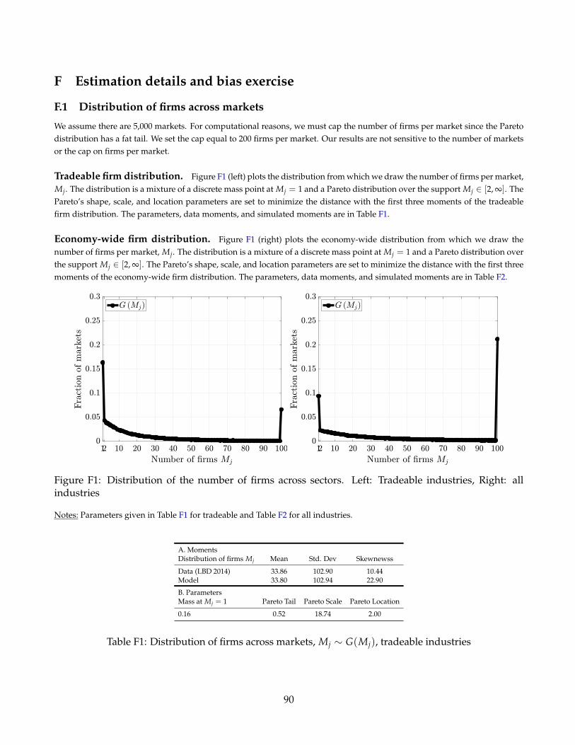
F Estimation details and bias exercise

F.1 Distribution of firms across markets

We assume there are 5,000 markets. For computational reasons, we must cap the number of firms per market since the Paretodistribution has a fat tail. We set the cap equal to 200 firms per market. Our results are not sensitive to the number of marketsor the cap on firms per market.

Tradeable firm distribution. Figure F1 (left) plots the distribution from which we draw the number of firms per market,Mj. The distribution is a mixture of a discrete mass point at Mj = 1 and a Pareto distribution over the support Mj ∈ [2, ∞]. ThePareto’s shape, scale, and location parameters are set to minimize the distance with the first three moments of the tradeablefirm distribution. The parameters, data moments, and simulated moments are in Table F1.

Economy-wide firm distribution. Figure F1 (right) plots the economy-wide distribution from which we draw thenumber of firms per market, Mj. The distribution is a mixture of a discrete mass point at Mj = 1 and a Pareto distribution overthe support Mj ∈ [2, ∞]. The Pareto’s shape, scale, and location parameters are set to minimize the distance with the first threemoments of the economy-wide firm distribution. The parameters, data moments, and simulated moments are in Table F2.

Figure F1: Distribution of the number of firms across sectors. Left: Tradeable industries, Right: allindustries

Notes: Parameters given in Table F1 for tradeable and Table F2 for all industries.

A. MomentsDistribution of firms Mj Mean Std. Dev Skewnewss

Data (LBD 2014) 33.86 102.90 10.44Model 33.80 102.94 22.90

B. ParametersMass at Mj = 1 Pareto Tail Pareto Scale Pareto Location

0.16 0.52 18.74 2.00

Table F1: Distribution of firms across markets, Mj ∼ G(Mj), tradeable industries

90

A. MomentsDistribution of firms Mj Mean Std. Dev Skewnewss

Data (LBD 2014) 113.10 619.00 26.14Model 113.14 618.82 36.08

B. ParametersMass at Mj = 1 Pareto Tail Pareto Scale Pareto Location

0.09 0.71 38.36 2.00

Table F2: Distribution of firms across markets, Mj ∼ G(Mj), all industries

F.2 Tax Experiment Details

In each simulation of the model, we conduct a tax experiment where we simulate a common corporate tax change of ∆τ =

τ′C − τC = .01, holding aggregate quantities fixed. We rerun our reduced-form regressions on the simulated data in orderto recover average reduced-form labor supply elasticities as a function of wage-bill shares. These market-share-dependentreduced-form labor supply elasticities are the moments used to recover η and θ in Section 2. We describe the details of theexercise below:

1. Simulate the benchmark equilibrium for two periods (date t = 0, 1) without taxes. Treat these observations as ‘data.’ Wemust simulate two prior periods in order to define the lagged wage-bill share of the firm in the market.

2. C-corps in the model economy (recall there is a share ωC of C-corps in all markets) have their taxes raised by 1 percentagepoint.

3. Simulate the ‘post-shock’ equilibrium, treat as date t = 2 ‘data.’

4. Estimate the same reduced-form regressions as Section 2 using the t = 0, 1, 2 simulated data. Estimate the followingregressions for each firm i in region j:

log(nijt) = αi + βnτCt + γ0ssijt−1 + βnsτCt ∗ sijt−1 + εijt

log(wijt) = αi + βwτCt + ω0ssijt−1 + βwsτCt ∗ sijt−1 + uijt

5. Compute the employment and wage elasticities with respect to productivity, d log(nijt)dτCt

and d log(wijt)dτCt

. Use these expres-sions to recover the average reduced-form labor supply elasticities using the formula:

ε(sijt−1) =βn + βnssijt−1

βw + βwssijt−1

6. Use the recovered ε(sijt−1), sijt−1 pairs as moments to recover η and θ.

F.3 Biases

To explore the difference between structural and reduced-form labor supply elasticities, we conduct a Monte Carlo exercisewhere we simulate a perfectly idiosyncratic shock and then compute reduced form elasticities. We average these across firmswithin payroll share bins and compare these to the structural labor supply elasticity implied by ε(sij) = [θ−1sij + η−1(1 −sij)]

−1. We repeat this exercise for 5,000 simulations and report the averages in Figure 6. We describe the details of the exercisebelow:

1. Simulate the benchmark equilibrium, treat as date t = 1 ‘data.’

2. Randomly select 1 firms in each market and increase their productivity by 1% (20% or 50%), holding aggregates fixed(assuming partial equilibrium).

3. Simulate ‘post-shock’ partial equilibrium (industry competitors adjust but aggregates are held fixed), treat as date t = 2‘data.’

91

4. Isolate firms with pre-shock wage-bill shares sij in bins with nodes [.1, . . . , .9]. Within each bin, compute the mean of∆ log(nijt)/∆ log(wijt) using the t = 1, 2 simulated data.

5. Figure 6 plots these values at the upper cutoff of these bins. For shares equal to 0 and 1, the solution is exact ε(1) =

ε(1) = θ, ε(0) = ε(0) = η.

F.4 Additional threats to consistency.

There are two additional threats to consistency of our simulations. (i) apportionment of state taxes across multi-state productionunits may mean that state corporate taxes do not affect firms within a state, and (ii) anticipation of tax changes. We discussthese issues in the context of prior analysis by Suárez Serrato and Zidar (2016) and Giroud and Rauh (2019).

First, Suárez Serrato and Zidar (2016) show that the impact of state corporate taxes on local economic activity is extremelysimilar for both (i) the statutory corporate taxes used here, and (ii) effective corporate taxes—i.e. ‘business taxes’—carefullyadjusted for apportionment weights.52 Since establishment sales and company property values are not available to us, wecannot construct accurate apportionment weights and thus we focus on statutory tax rates compiled by Giroud and Rauh(2019). We only require similarly sized firms to face similarly sized shocks. The magnitude of the shock is not important forour identification of η and θ, instead it is their relative employment to wage adjustment that identifies η and θ.

Second, both Suárez Serrato and Zidar (2016) and Giroud and Rauh (2019) establish that including various aspects ofchanges to fiscal policy around corporate tax adjustments have negligible affects on their measured elasticities of local economicactivity to state corporate taxes.53 We interpret this as indirect evidence that the reforms are not paired with other predictablecomponents of fiscal stimulus, such as unemployment insurance, which follow time-invariant threshold rules and are typicallytriggered in recessions (e.g. Mitman and Rabinovich (2019)).

G Discussion of empirical estimation and robustness

This section is divided into three parts. First, a discussion of how our empirical strategy relates to other papers in the literature.Second, including exit in our regressions and re-estimating the model under exit. Third, a set of robustness exercises aroundstate-level omitted variables, non-wage compensation, variation in capital intensity, and an alternative approach using ‘direct’elasticities.

G.1 Discussion

As discussed in Section 1.4, the model predicts that the labor supply elasticity faced by firms varies by their market share.If this relationship were known in the data, it would precisely pin down the elasticities of substitution of labor within andacross sectors. Existing work estimating labor supply elasticities to firms has focused either on specific markets (e.g. (Webber,2016) or in well identified responses to small experimental variations in wages (Dube, Jacobs, Naidu, and Suri, 2020; Dube,Cengiz, Lindner, and Zipperer, 2019). A contribution of this paper is to estimate a share-elasticity relationship through a novelquasi-natural experiment using a large cross-section of firms.

The intuition for our procedure is as follows. We first estimate the rate at which labor demand shocks pass-through to wagesand employment and the reduced-form relationship between these labor supply elasticities and local labor market shares. Wethen invert this empirical relationship using our model to recover estimates of the structural parameters that control the relativesubstitutability of labor within and between markets. To identify how pass-through rates vary by market share, we compare

52See their discussion of Table A21, p.19 (emphasis added): “Column (6) of Table 5 and Appendix Table A21 show that usingstatutory state corporate tax rates in Equation 21 (instead of business tax rates τb) results in similar and significant estimates,indicating that our measure of business tax rates is not crucial for the results.”

53Giroud and Rauh (2019) establish the plausible exogeneity of state-corporate tax changes. From a public finance perspec-tive they study the effects of state corporate tax changes on employment and wages. Their focus is within firm, across stateresponses, and the reallocation of firm employment across states following tax changes. For an exhaustive description of thesetax changes we point the interested reader to their paper.

92

how the firm responds to these labor demand shocks differentially across markets within the same state, but in which theirshares of the labor market differ.

This procedure requires a shock to labor demand in order to trace out the labor supply curve. We use state corporate taxchanges which constitute a shock to firm labor demand via their distortion of accounting profits relative to economic profits,shifting the marginal revenue product of labor.54 Both Suárez Serrato and Zidar (2016) and Giroud and Rauh (2019) havestudied the impact of state-level corporate tax shocks on local economic activity. We address three issues that may arise: (i)apportionment of state taxes across multi-state production units may mean that state corporate taxes do not affect firms withina state, (ii) taxes are anticipated, (iii) such shocks affect all firms in a region and so can only be used to identify θ.

First, Suárez Serrato and Zidar (2016) show that the impact of corporate taxes on local economic activity is extremely similarfor both (i) the statutory corporate taxes that we use and (ii) effective corporate taxes adjusted for apportionment weights.55

Since establishment sales and company property values are not available to us, we focus on statutory taxes rates compiled byGiroud and Rauh (2019) and based on Suárez Serrato and Zidar (2016) we do not adjust for the apportionment regime of thestate.

Second, both Suárez Serrato and Zidar (2016) and Giroud and Rauh (2019) establish that the inclusion of other aspects ofchanges to fiscal policy around the corporate tax changes does not affect their measured elasticities of local economic activityto corporate taxes.56

Third, the fact that (i) only C-corps pay statutory corporate tax rates, (ii) the structure of our model and (iii) Monte Carloexercises, provide support that we may infer η and θ from a shock that affects some but not all firms. We briefly discuss this inmore detail.

G.2 Exits

G.2.1 Empirics

In Table G1, we estimate linear probability models of firm-market exit in year t + 1 as a function of corporate taxes in yeart. In column (1) and (2), we find economically insignificant results. This complements the work of Giroud and Rauh (2019),who aggregate plants at the firm-state level and study how the number of plants per C-Corp in a state responds to corporatetax changes. Since our relevant level of economic activity is at the firm-market level, and since we are interested in exits fromthe market entirely, we use a different approach. We regress whether a firm exits a firm-market entirely, instead of simplyregressing the number of plants in the state on the tax change. Our results do not necessary contradict Giroud and Rauh (2019).Giroud and Rauh (2019)’s results imply that firms may adjust the number of plants in the state. Our results imply that firms donot appear to be exiting markets entirely in response to a corporate tax change.

G.2.2 Model re-estimation with exit

Our empirical results suggest that exits are not a threat to our exercise. Nonetheless, we show that our model estimates of η

and θ are robust under the assumption that 5% of C-Corps exit. This is an extreme and counterfactually high exit response tocorporate tax hikes. Table G2 reports the results. Our estimates of η and θ are similar to the baseline.

54We have not included corporate taxes in our benchmark model. We show that the mapping of our model to the data doesnot require us to take a stance on the transmission mechanism linking corporate taxes to productivity. Nevertheless, AppendixE.9 shows how corporate tax rates map to shocks to the marginal revenue productivity of labor in our framework.

55See their discussion of Table A21, p.19 (emphasis added): “Column (6) of Table 5 and Appendix Table A21 show that usingstatutory state corporate tax rates in Equation 21 (instead of business tax rates τb) results in similar and significant estimates,indicating that our measure of business tax rates is not crucial for the results.”

56Giroud and Rauh (2019) establish the plausible exogeneity of state-corporate tax changes. From a public finance perspec-tive they study the effects of state corporate tax changes on employment and wages. Their focus is within firm, across stateresponses, and the reallocation of firm employment across states following tax changes. For an exhaustive description of thesetax changes we point the interested reader to their paper.

93

(1) (2)Exitijt+1 Exitijt+1

τs(j)t -0.000447 -0.000938(0.000556) (0.000771)[0.000168] [0.000194]

Fixed Effects Market, Year Firmid, Market, YearR-squared 0.042 0.218Observations 2.844e+06 2.844e+06

Table G1: Exit probability

Notes: According to Census requirements, the number of observations is rounded to the nearest 1,000. Standard errors inround parentheses (·) are clustered at State × Year level. Standard errors in square parentheses [·] are clustered at Market ×Year level. Sample includes tradeable C-Corps from 1977 to 2011.

η θ

Benchmark 6.96 0.45Exit rate 5% 8.17 0.43

Table G2: Re-estimation of the model assuming 5% of firms exit the market in response to a corporatetax hike of 1%.

G.3 Regression Robustness

We discuss robustness of our regression specifications and their implications for the relationship between market shares andreduced form labor supply elasticities. We consider (i) state-level omitted variables, (ii) compute direct elasticities at the firmlevel, (iii) account for systematic variation in non-wage compensation, (iv) account for systematic variation in capital intensity.

G.3.1 State-level omitted variables

Model estimation simply requires consistent auxiliary moments that can be simulated. The threat to consistency when we esti-mate equation 13 is that there are other forces moving employment and wages at the state-year level, e.g. tax cuts occur in boomyears etc. To control for state-level responses, Giroud and Rauh (2019) include S-Corps as a control for C-Corps. Through thelens of our theory, S-Corps do not provide a suitable control group, since they respond to the treatment as well. Thus, the stableunit treatment value assumption (SUTVA) is violated. To alleviate concerns that our estimates are being driven by omittedstate-year level variation, we include specifications which include both state×year fixed effects as well as firmid×market fixedeffects. State-level corporate tax changes are subsumed in the fixed effects, and so we are only able to identify the interactionbetween corporate taxes and wage-bill shares. Table G3 illustrates our results. Comparing columns (1) through (4) in TableG3 to Table 1, we find very similar interactions between taxes and wage-bill shares for both date t and t + 1 employment andwages. We view these results as suggestive evidence that omitted variables at the state-year level are unlikely to explain ourresults.

G.3.2 Direct elasticities

To provide further evidence that labor supply elasticities decline as a function of a firm’s wage-bill share, we directly computethe ratio of wage changes to employment changes at the firm-level and we study their relationship to a firm’s wage-bill share.To allow for perfect competition (non-zero employment change with zero wage change), we compute the inverse elasticityat the firm level ∆wijt

∆nijt

nijtwijt

between year t and t + 1. To measure an elasticity, we require a supply or demand shifter. We usecorporate tax changes as demand shifters. These ‘direct’ elasticities include significant amounts of measurement error. Inparticular, the measurement error in the denominator results in many extreme outliers. We impose several criteria to deal with

94

(1) (2) (3) (4)log nijt log wijt log nijt+1 log wijt+1

sijt−1 0.894*** 0.113*** 0.723*** 0.0959***(0.0206) (0.00982) (0.0202) (0.0107)[0.0159] [0.00898] [0.0165] [0.0100]

τs(j)t × sijt−1 0.0169*** 0.00739*** 0.0159*** 0.00760***(0.00275) (0.00127) (0.00268) (0.00133)[0.00199] [0.00112] [0.00208] [0.00125]

Fixed effects Y Y Y YR-squared 0.897 0.791 0.876 0.736Round N 2.844e+06 2.844e+06 2.844e+06 2.844e+06

Table G3: State-year fixed effects

Notes: All specifications include fixed effects for: (i) year, (ii) firmid×market, and (iii) state×year. According to Censusrequirements, the number of observations is rounded to the nearest 1,000.

this measurement error. First, we require an employment adjustment of at least ±5 employees.57 Second, we only use taxchanges of at least half of a percentage point |∆τs(j)t| > .5. Third, we winsorize the dependent variable at the .5% level.58

Fourth, to remove common state-year fluctuations in wages and employment, we include state-year fixed effects as well asfirm-market fixed effects.

To isolate the size-dependent labor supply elasticity, we interact the corporate tax changes with the firm’s wage-bill share.

Because of the high-dimensional firm must adjust employment twice by at least ±5 employees between 1977 to 2011 in order

for our fixed effects to be estimated. We run specifications of the following form:

[εData(s)]−1 =∆wijt

∆nijt

nijt

wijt= αij + γs(j)t + β11(sijt−1 ∈ [.01, .05)) + β21(sijt−1 ∈ [.05, 1]) (G1)

+ β31(|∆τs(j)t| > .5)× 1(sijt−1 ∈ [.01, .05)) + β41(|∆τs(j)t| > .5)× 1(sijt−1 ∈ [.05, 1]) + εijt

Table H4 provides estimates of equation (H1). Column (1) shows that the inverse elasticity for firms with wage bill sharesbetween 1% and 5% is significantly different from those whose wage-bill shares are less than 1%. Their inverse elasticity is.0476 percentage points greater. Based on our estimates in Table 2, if firms with a wage-bill share less than 1% have a laborsupply elasticity of 2, then these estimates imply that firms with a wage bill share between 1% and 5% have a labor supplyelasticity of roughly 1.83. For those with wage-bill shares greater than 5%, their inverse elasticity increases by 0.075 percentagepoints relative to those with a wage-bill share less than 1%. Based on our estimates in Table 2, if firms with a wage-bill shareless than 1% have a labor supply elasticity of 2, then these estimates imply that firms with a wage bill share greater than 5%have a labor supply elasticity of roughly 1.74. Lastly, column (2) estimates the inverse labor supply elasticity using changes inemployment and wages between t and t + 2, while keeping the same and all other right-hand-side regressors in equation (H1)the same. We interpret column (2) as a long-run inverse labor supply elasticity. Relative to the omitted group of firms withshares less than 1%, we find that firms with wage-bill shares greater than 5% have an inverse elasticity that is 0.0959 percentagepoints greater. Based on our estimates in Table 2, if firms with a wage-bill share less than 1% have a labor supply elasticity of2, then these estimates imply that firms with a wage bill share greater than 5% have a labor supply elasticity of roughly 1.68.These estimates are remarkably close to our linear regression estimates in Section 2.2. Figure H4 graphically depicts the inverseelasticity [εData(s)]−1 =

∆wijt∆nijt

nijtwijt

relative to the omitted group of firms with wage-bill shares less than 1%.

57We also tried cutoffs of 3, 7, 10 and our results are robust.58We also tried winsorizing at the 1% and 5% levels and our results are robust.

95

Figure G1: Inverse elasticitiesNotes: Point estimates plotted from Table H4. See text for details.

G.3.3 Non-wage compensation

Can our results be attributed to non-wage benefits that vary by size? We argue no. We find that while benefits covary positivelywith wage-bill share, they cannot explain the magnitude of size-dependent markdowns we estimate in the data.

To bound the effect of benefits on our markdowns, we must measure the elasticity of benefits with respect to the wage-bill share of the firm. The Census of Manufacturers includes data on worker benefits in recent survey waves. We use the2012 Census of Manufacturers to estimate how benefits per employee varies with local wage-bill shares. To mitigate spuriouscorrelations between market-share and benefits, we include firm fixed effects. Thus our empirics compare within a firm, acrossplants, how local wage-bill shares covary with benefits. Table H3 includes our results. We find that a 1 percentage point increasein the wage bill share results in a 0.597% increase in benefits per worker. We repeat the exercise after winsorizing benefits perworker at the 1% level, and we find a very similar elasticity; thus, our low elasticity of benefit per worker with wage-bill shareis not driven by outliers.

Figure H3 plots the elasticity of the model’s markdowns as a function of the wage-bill share. For wage-bill shares of 1%,the elasticity of the wage-bill share is close to -6%. Thus non-wage benefits are too small to be responsible for our estimatedmarkdown elasticities.

G.3.4 Capital Intensity

The Census of Manufacturers includes data on assets per employee.59 We use the 2012 Census of Manufacturers to estimatehow assets per employee varies with local wage-bill shares. We include firm (firmid) fixed effects to isolate within-firm, across-plant variation in the way assets per employee covaries with local wage-bill shares. Table H3 includes our results. We find thata 1 percentage point increase in the wage bill share results in a 0.176% increase in assets per employee. Our mean value of assetsper employee in this sample of multi-plant firms is $332,500. Thus a 1 percentage point increase in wage-bill share correspondsto an increase in assets of $595 for the average firm. We view this as economically insignificant. Column (2) removes outliers bywinsorizing the data at the 1% level. We find a slightly larger elasticity, however, we view these results as supportive evidencethat our size-dependent labor supply elasticities cannot be explained by differential capital adjustment.

59We use beginning-of-year asset values.

96

(1) (2)Inverse elasticity t to t + 1 Inverse elasticity t to t + 2

1(|∆τs(j)t| > .5)× sijt−1 ∈ [.01, .05) 0.0476** -0.00314(0.0208) (0.0409)[0.0221] [0.0421]

1(|∆τs(j)t| > .5)× sijt−1 ∈ [.05, 1] 0.0741** 0.0959*(0.0354) (0.0560)[0.0300] [0.0517]

Fixed Effects Yes YesR-squared 0.257 0.225N 722000 722000

Table G4: Estimation results for equation (H1)

Notes: All specifications include fixed effects for: (i) year, (ii) firmid×market, and (iii) state×year. According to Censusrequirements, the number of observations is rounded to the nearest 1,000. Standard errors in round parentheses (·) areclustered at State × Year level. Standard errors in square parentheses [·] are clustered at Market × Year level. Sample includestradeable C-Corps from 1977 to 2011.

(1) (2)Log benefits per employeeijt Log benefits per employeeijt,

1% winsorized

swnijt 0.00597*** 0.00565***

(0.000261) (0.000241)

R-squared 0.687 0.688N 36000 36000

Table G5: Benefits per employee and wage-bill shares

Notes: All specifications include fixed effects for: (i) year, (ii) firmid , and (iii) market. According to Census requirements, thenumber of observations is rounded to the nearest 1,000. Standard errors clustered at the firmid level. Sample includestradeable Census of Manufacturers firms in 2012.

(1) (2)Log assets per employeeijt Log assets per employeeijt, 1% winsorized

swnijt 0.00176** 0.00193***

(0.000749) (0.000693)

R-squared 0.639 0.638Observations 36000 36000

Table G6: Assets per employee and wage-bill shares

Notes: All specifications include fixed effects for: (i) year, (ii) firmid , and (iii) market. According to Census requirements, thenumber of observations is rounded to the nearest 1,000. Standard errors clustered at the firmid level. Sample includestradeable Census of Manufacturers firms in 2012.

97

Figure G2: Non-wage benefits and wage-bill shares

98