working paper n 91 | 2021 - bcra

Working Paper N 91 | 2021Alternative Monetary-Policy Instrumentsand Limited Credibility: An Exploration

Economic ResearchWorking Papers | 2021 | N 91

Alternative Monetary-Policy Instruments and Limited Credibility: An Exploration

Javier García-CiccoBanco Central de la República Argentina

April 2021

2 | BCRA | Working Papers 2017

Working Papers, N 91

Alternative Monetary-Policy Instruments and Limited Credibility: An Exploration

Javier García-CiccoBanco Central de la República Argentina

April 2021ISSN 1850-3977Electronic Edition

Reconquista 266, C1003ABFCiudad Autónoma de Buenos Aires, ArgentinaPhone | 54 11 4348-3582Email | [email protected] | www.bcra.gob.ar

The opinions expressed in this paper are the sole responsibility of its authors and do not necessarily represent the position of the Central Bank of Argentina. The Working Papers series is comprised of preliminary material intended to stimulate academic debate and receive comments. This paper may not be referenced without authorization from the authors.

NON-TECHNICAL SUMMARY

Research Question

The increasing use of inflation-targeting frameworks in developed and some emerging countrieshas influenced the literature to focus on monetary policy rules that use a short-term interestrate as the main instrument. However, this emphasis is not representative of the way monetarypolicy is implemented around the world. For example, according to IMF AREAER database, in2018 only 21% of a total of 192 countries had an inflation-targeting framework in place (usinga short-term rate as the instrument). The others were divided between countries that use anexchange-rate anchor (41%), those who target monetary aggregates (14%), and the remainder24% use some hybrid framework. This distribution is largely determined by policies in low-income and emerging economies.

At the same time, most studies analyzing rules for interest rates assume rational expectations.Such a setup presumes a high degree of credibility, since it poses that agents know the policyrule and believe it holds not only in the present but in the future as well. However, many low-income and emerging countries face situations with limited credibility. The goal of this paper isto understand the extent to which instrument choice depends on the degree of credibility.

Contribution

The comparison is performed by means of a small and open economy model with price and wagerigidities. To capture limits to credibility, we assume that inflation-related expectations are notrational. Instead, they are determined by econometric models that use past data to forecastthe future (a framework named adaptive learning). In particular, the role that exchange ratemovements may have in changing medium- and long-term inflation expectations is emphasized.In this context, three simple policy rules are compared: one for the interest rate (a Taylor rule),one for the growth rate of a monetary aggregate, and an exchange rate peg. The aim is tounderstand the pros and cons of using each of them when the economy is facing a shock toexternal borrowing costs.

Results

The benefits and costs of these alternatives depend largely on the credibility framework. Withhigh credibility (rational expectations) there is a trade-off between the dynamics of activityand inflation when a rule for the interest rate and one for money growth are compared, whilemaintaining a peg is costly. However, with limited credibility (adaptive learning), if exchange-rate surprises persistently change inflation expectations, the potential benefits of money-basedrules are more limited. Conversely, reducing exchange-rate volatility may be desirable to limitthe costs associated with un-anchored expectations.

Alternative Monetary-Policy Instruments and

Limited Credibility: An Exploration∗

Javier Garcıa-Cicco (BCRA)

Abstract

We evaluate the dynamics of a small and open economy under alternative simple rules for

different monetary-policy instruments, in a model with imperfectly anchored expectations.

The inflation-targeting consensus is that interest-rate rules are preferred, instead of using

either a monetary aggregate or the exchange rate; with arguments usually presented under

rational expectations and full credibility. In contrast, we assume agents use econometric

models to form inflation expectations, capturing limited credibility. In particular, we em-

phasize the exchange rate’s role in shaping medium- and long-term inflation forecasts. We

compare the dynamics after a shock to external-borrowing costs (arguably one of the most

important sources of fluctuations in emerging countries) under three policy instruments: a

Taylor-type rule for the interest rate, a constant-growth-rate rule for monetary aggregates,

and a fixed exchange rate. The analysis identifies relevant trade-offs in choosing among al-

ternative instruments, showing that the relative ranking is indeed influenced by how agents

form inflation-related expectations.

Resumen

Evaluamos las dinamicas de una economıa pequena y abierta bajo distintas reglas simples

para instrumentos de polıtica monetaria alternativos, en un modelo donde las expectativas

de inflacion no estan ancladas. En esquemas de metas de inflacion, el consenso se inclina por

reglas para la tasa de interes, en lugar de utilizar agregados monetarios o el tipo de cambio,

usando argumentos que generalmente asumen expectativas racionales y completa credibili-

dad. En cambio, asumimos aquı que los agentes usan modelos econometricos para formar

expectativas de inflacion, capturando ası credibilidad limitada. En particular, enfatizamos el

rol del tipo de cambio para determinar las expectativas de inflacion de mediano y largo plazo.

Comparamos los efectos de shocks al costo de endeudamiento externo (que tienen un papel

relevante como determinante de ciclos en economıas emergentes) bajo tres polıticas alterna-

tivas: una regla de Taylor para la tasa de interes, una meta de crecimiento para agregados

monetarios, y un tipo de cambio fijo. El analisis permite identificar costos y beneficios de los

distintos instrumentos, enfatizando que la valoracion relativa de las alternativas es sensible

a la forma en que los agentes forman expectativas de inflacion.

∗This paper benefited from comments by Ozge Akinci, Jose De Gregorio, Gianlucca Begnino, and participants inthe 5th BIS-CCA Research Network on “Monetary Policy Frameworks and Communication,” and the LIV AnnualMeeting of the Economic-Policy Association of Argentina. E-mail: [email protected]

[email protected]

1 Introduction

This paper presents an exploration of the trade-offs associated with choosing alternative monetary-

policy instruments in small and open economies, in a context of imperfectly anchored expectations

or limited credibility. Along with the increased popularity of inflation targeting as a policy frame-

work, the vast majority of studies analyzing policy rules focus on a short-term interest rate as the

instrument, in a context of rational expectations (where agents believe the policy rule holds not

only in the present but also in the future, a strong form of policy credibility).1 Even those papers

relaxing the rational-expectations assumption mostly focus on interest-rate rules.2 An exception

that has received some attention is the complementary role of exchange-rate interventions under

inflation targeting, but still maintaining the policy rate as the main instrument.3

This predominance of studies analyzing interest-rate rules is not representative of the way

policy is conducted around the world. According to the IMF AREAER database, in 2018 only

21% of a total of 192 countries had an inflation-targeting framework (all of them using a policy

rate as the main instrument), while 14% implemented a monetary-target setup, 41% had an

exchange-rate anchor in place, and the remainder 24% implemented some other hybrid setup.

This distribution is mostly influenced by the behavior of low-income and emerging countries (e.g.

no developed economy has a monetary target in place). Moreover, 15% of those implementing

inflation targeting choose to de facto manage the exchange rate to some extent, while close to 80%

among those under a money-target also actively intervene in the foreign exchange market.

Our goal is to understand if limited credibility could be a determinant of instrument choice; for

in many contexts credibility cannot be taken for granted. This has been historically the case at the

initial stages of inflation-stabilization programs. Indeed, an earlier literature analyzes the dynamics

of stabilization plans under alternative policy instruments; see, for instance, the surveys in Calvo

and Vegh (1994, 1999). More recently, Calvo (2018) presents concerns about implementing an

interest-rate-based inflation targeting to generate a permanent reduction in inflation. Taylor (2019)

also indicates that some type of monetary target might be desirable under lack of credibility even

if the goal is to achieve an inflation target.

The analysis begins with a baseline model of a small and open economy with incomplete fi-

nancial markets, nominal rigidities in prices and wages, dominant-currency pricing, and capital

accumulation. To account for limited credibility, we deviate from rational expectations by as-

suming that agents use econometric models (based only on past data) to form inflation-related

expectations. This choice is motivated by previous studies that highlight how adaptive learning

might limit the impact of monetary policy.4 In particular, the forecasting model is a VAR with

a time-varying mean, such that news can have a persistent impact if they modify the inference

about long-run inflation.

1Some examples in closed economy models are Schmitt-Grohe and Uribe (2007), Faia (2008), Faia and Monacelli(2007), Taylor and Williams (2010); while for open economies some relevant references are Faia and Monacelli(2008), De Paoli (2009), Corsetti et al. (2010), Devereux et al. (2006), Lama and Medina (2011). Notable exceptionsare Berg et al. (2010) and Andrle et al. (2013), analyzing hybrid rules for low-income countries with a role formonetary aggregates.

2For instance, Erceg and Levin (2003), Cogley et al. (2015), Gibbs and Kulish (2017), among others.3See, for instance, Ghosh et al. (2016) in the context of rational expectations and Adler et al. (2019) in a model

where agents learn about possible changes in the inflation target (in the spirit of Erceg and Levin, 2003).4Surveys of this literature can be found in Gaspar et al. (2010) and Eusepi and Preston (2018b), among others.

1

We emphasize two different components of the learning process. The first appears if long-run

inflation expectations are shaped by past inflation only, which has been the main focus in most of

the related literature (particularly in closed-economy setups). This has two main consequences:

inflation is more persistent and, as inflation expectations also affect the real rate relevant for

inter-temporal decisions, the power of the central bank to impact aggregate demand is limited.

The second component is specific to open economies and is related to exchange-rate volatility.

The literature has extensively explored the role of exchange rates in shaping inflation dynamics

(see, for instance, the survey in Burstein and Gopinath, 2014). Besides the several general-

equilibrium channels emphasized elsewhere, here we consider the possibility that medium- and

long-run inflation expectations are directly influenced by exchange-rate surprises. While this link

has not been explored in the literature to the best of our knowledge, there is some suggestive

evidence of such an effect. For instance, both the cross-country and time-variation of exchange-

rate-pass-through measures seem to correlate with metrics of monetary-policy credibility (e.g.

Carriere-Swallow et al., 2016). Moreover, in general equilibrium the exchange-rate-pass-through is

influenced by expected monetary policy (as stressed by Garcıa-Cicco and Garcıa-Schmidt, 2020).

Finally, Adler et al. (2019) show that, among inflation targeters, countries with relatively low

credibility tend to intervene more actively and frequently in the foreign exchange market.

To further explore this possibility, we analyze market-expectations data for both Argentina

and Chile, two cases with arguably different degrees of credibility. We find reduced-form evidence

that large exchange-rate surprises significantly change one-year-ahead inflation expectations in

Argentina but not in Chile. While additional evidence is required to study this link, our model-

based analysis suggests that dynamics and policy prescriptions can significantly change if, due to

limited credibility, agents adjust long-term inflation expectations after exchange-rate jumps.

We compare the dynamics in our model under different expectation-formation assumptions,

contrasting three policy alternatives: a Taylor-type rule for the short-term interest rate, a constant

growth rate for base money, and an exchange-rate peg. We focus on the role these rules have in

smoothing the responses after an unexpected rise in foreign-financing costs; an important driving

force behind fluctuations in emerging countries (e.g. Uribe and Yue, 2006, among many others).

Moreover, external interest rates are also key drivers of exchange-rate movements, which in turn

shape inflation dynamics.

The comparison under rational expectations shows that, qualitatively, there is a trade-off in

choosing between an interest-rate and a constant-money-growth rule. Limiting fluctuations in the

quantity of money partially insulates activity-related variables from the contractionary effects of

the external shock, while at the same time increases its inflation volatility. This is due to the

different behavior of interest rates under both policy configurations. Moreover, welfare compar-

isons indicate that the money-growth rule is marginally preferred. Instead, a peg induces a larger

contraction following the negative external shock, without a clear advantage in the inflationary

front, and it is more costly in welfare terms.

In the limited-credibility setup where only past inflation influences long-run expectations, the

qualitative trade-offs between the three rules are still present, but quantitatively the differences

are exacerbated. This is a consequence of (i) a more persistent inflation and (ii) a magnified effect

of interest-rate changes in activity if expectations are not fully rational. In welfare terms, the

interest-rate rule is preferred to the other alternatives.

2

When exchange-rate movements can directly affect long-term inflation expectations, the dy-

namics under different rules are modified. The dampening effect on activity obtained with a

constant money growth is limited: the dynamics of GDP under interest-rate and money rules

are closer to each other. At the same time, a money-based rule generates the worst outcomes

in terms of inflation, as it induces more exchange-rate volatility. Finally, limiting exchange-rate

fluctuations might be useful to prevent significant shifts in medium- and long-term expectations:

the welfare cost of a peg is halved in this learning setup.

We also show that these results are maintained if we add several relevant features to the

model. In particular, we consider financial frictions in the form of an endogenous foreign-financing

spread; habits at the good-level further limiting the expenditure-switching channel; a domestic

banking sector that yields a richer structure for monetary aggregates; a fraction of households with

restricted access to financial markets; and a final version combining all of them. Among the main

results, financial frictions further emphasize the potential gains from exchange-rate smoothing in

situations where exchange-rate jumps can feed into long-term expectations. Also, the relative

ranking of alternatives can be different for constrained and unconstrained households, particularly

under limited credibility.

The rest of the paper is organized as follows. Section 2 presents the baseline model, with a

detailed discussion of the learning framework and its calibration. Section 3 compares the alterna-

tive policy instruments in the context of rational expectations. Section 4 performs the comparison

under limited credibility. Section 5 explores the sensitivity if the aforementioned characteristics

are added to the model. Finally, Section 6 concludes.

2 Baseline Model

The setup is one of a small and open economy with free international capital mobility and in-

complete financial markets. There are several goods: home, imported and final goods, as well

capital. The home good is produced by combining labor and capital. The final consumption

good is composed of home and imported goods. The markets for final goods and labor have a

monopolistic-competitive structure, where prices are subject to Calvo-style frictions. Exports are

not sensitive to real exchange rate fluctuations as in the dominant-currency-pricing paradigm.

Households derive utility from consumption, leisure, and money holdings. They also have access

to international borrowing and treasuries. The rest of this section describes the different agents in

the model, the general equilibrium conditions, the assumptions regarding expectations formation,

and the alternative policy rules considered.

3

2.1 Households

Households seek to maximize,5

E0

∞∑

t=0

βtU

(ct, ht,

Mt

Pt

),

subject to the constraint

Ptct + StB∗,Ht +BT

t +Mt + Tt ≤ Wtht +Mt−1 + StB∗,Ht−1R

∗

t−1 +BTt−1Rt−1 + Ωt.

Here, ct denotes consumption, ht are hours worked, B∗,Ht are holdings of foreign bonds (with inter-

est rate R∗

t ), BTt are holdings of domestic treasuries (with rate Rt), Mt denotes money holdings,

Tt are lump-sum transfers, St is the nominal exchange rate, Pt is the price of final consumption

goods, Wt is the nominal wage, and Ωt denotes profits from the ownership of firms.6

Letting βt λt

Ptdenote the Lagrange multiplier associated with the resource constraint, we obtain

the following optimality conditions

λt = Uc,t, λt = βR∗

tEt

πst+1λt+1

πt+1

,

λt = βRtEt

λt+1

πt+1

,

UMP,t

λt= 1− 1

Rt,

where Ux,t =∂Ut

∂xt, wt ≡ Wt

Pt, πt ≡ Pt

Pt−1, and πs

t ≡ St

St−1. The first relates the Lagrange multiplier

with the marginal utility of consumption. The second and third characterize the inter-temporal

trade-off in choosing domestic and foreign bonds, while the last represents the demand for money.

Additionally, define the stochastic discount factor for claims in domestic currency as χt,t+s =

βs λt+s

λt

Pt

Pt+s.

Labor decisions are made by a central authority (e.g. a union) which supplies labor monopolis-

tically to a continuum of labor markets indexed by i ∈ [0, 1]. Households are indifferent between

working in any of these markets, and there are no differences in the quality of labor provided by the

different types of households. In each of these markets the union faces a demand for labor given

by hit = [Wit/Wt]−ǫW hdt , where Wit denotes the nominal wage charged by the union in market

i, Wt is an aggregate hourly wage index that satisfies (Wt)1−ǫW =

∫ 1

0W 1−ǫW

it di, and hdt denotes

aggregate labor demand by firms. The union takes Wt and hdt as given and, once wages are set,

it satisfies all labor demanded. In addition, the total number of hours allocated to the different

labor markets must satisfy the resource constraint ht =∫ 1

0hitdi.

Wage setting is subject to a Calvo-type problem, whereby each period the union can set its

5While functional forms are presented in Appendix A, it is worth mentioning that we assume preferencesfeature no wealth-effects in labor supply, external habits in consumption and money holdings, and inter-temporalconsumption decisions that are independent from labor and money.

6Throughout, uppercase letters denote nominal variables containing a unit root in equilibrium (due to long-runinflation), while lowercase letters indicate stationary variables. Variables without time subscript denote non-stochastic steady-state values in the stationary model. Finally, we use the notation xt ≡ ln(xt/x) for a genericvariable xt.

4

nominal wage optimally in a fraction 1− θW of randomly chosen labor markets, and in the other

markets the past wage is indexed to a generic indexation variable πI,Wt = (πt−1)

ϑW (π)1−ϑW . In

other words, wage indexation depends on past- and steady-state inflation.

Under this setup, labor supply is characterized by two equations. One describing the trade-off

between consumption and labor, given by

wtmcWt =

−Uh,t

λt,

where mcWt is the relevant marginal cost for wage-related decisions (i.e. the gap in the efficient

allocation). The other is the Wage Phillips curve, which after log-linearization around the non-

stochastic steady state yields

(πWt − ϑW πt−1

)= βEt

πWt+1 − ϑW πt

+

(1− θW )(1− θWβ)

θWmcWt ,

where πWt = Wt

Wt−1.

2.2 Final and Home Goods

Final goods are produced in two stages. At a wholesale level, a set of competitive firms combine

home (xHt ) and foreign goods (xFt ) using the production function:

yCwt =

[ω1/η

(xHt

)1−1/η+ (1− ω)1/η

(xFt

)1−1/η] η

η−1

. (1)

Nominal profits are given by PCwt yCw

t − PHt x

Ht − P F

t xFt , leading to the following demands:

xFt = (1− ω)

(pFtpCwt

)−η

yCt , xHt = ω

(pHtpCwt

)−η

yCt .

with pFt ≡ P Ft /Pt, p

Ht ≡ PH

t /Pt, pCwt ≡ PCw

t /Pt.

The retail level features a monopolistic-competitive structure. The production yCt is a combina-

tion of a continuum of varieties indexed by j ∈ [0, 1] using the technology yCt =[∫ 1

0

(xCjt

)1− 1

ǫ dj] ǫ

ǫ−1

,

leading for the following demand for variety j,

xCjt =

(Pjt

Pt

)−ǫ

yCt .

The producer of a given variety j internalizes this demand, purchases wholesale final goods at

price PCwt , and transforms into the variety j using a linear technology (yCjt = xCw

jt ). In setting prices,

she faces a Calvo probability of not being able to optimally change its price given by θ. Whenever

she is not able to choose optimally, the previous-period price is indexed by πIt = (πt−1)

ϑ(π)1−ϑ.

After a log-linearization we obtain the following Phillips curve

(πt − ϑπt−1) = βEt πt+1 − ϑπt+(1− θ)(1− θβ)

θpCwt ,

5

2.3 Home Goods

These are produced competitively by combining labor (ht) and capital (kdt ) according to the

production function

yHt = zt(hdt )

α(kdt )(1−α).

where zt is an exogenous productivity shock. Profit maximization leads to the following input

demands:

pHt ztα

(yHthdt

)= wt, pHt zt(1− α)

(yHtkdt

)= rKt ,

where RKt is the rental price of capital, and rKt = RK

t /Pt. In equilibrium, kdt = kt−1 and hdt = ht.

2.4 Capital Goods and Investment

Capital accumulation is organized in two steps. A first set of competitive firms buy used capital,

(1− δ)kt−1, and combine it with final goods (it) to produce new capital (kt), using the technology

kt = (1− δ)kt−1 +

[1− S

(itit−1

)]it.

where S(·) denotes investment-adjustment costs satisfying S(1) = 0, S ′(1) = 0, and S ′′(·) > 0.

Profit maximization leads to the following optimality condition

1 = qt

[1− S

(itit−1

)− S ′

(itit−1

)itit−1

]+ Et

βλt+1

λtqt+1S

′

(it+1

it

)(it+1

it

)2,

where qt = Qt/Pt is the relative price of capital goods.

In the second stage, another set of competitive firms rent the stock of capital to firms and, after

depreciation, sell the used capital to capital-goods producers. Afterward, they buy new capital

for the next period. The optimal choice of these firms is,

1 = Et

χt,t+1

[πt+1[r

Kt+1 + (1− δ)qt+1]

qt

].

2.5 Fiscal and Monetary Policy

The consolidated balance sheet of the government is given by

Ptgt = (Mt −Mt−1) + St

(B∗,T

t − R∗

tB∗,Tt−1

)+(BT

t −Rt−1BTt−1

)+ Tt.

where gt is an exogenous process. In this setup, Tt adjust to satisfy this constraint (fiscal policy

is passive) and thus Ricardian equivalence holds (only gt matters for equilibrium determination).

In turn, the monetary authority set its policy by choosing a rule for either instrument Rt, Mt, or

πSt ; which are discussed below.

6

2.6 Rest of the World

The domestic economy has several interactions with the rest of the world. First, interest rates are

given by

R∗

t = RWt exp

φ(−b∗t + b

). (2)

where RWt denotes the world interest rate and the second term is a debt elastic premium (with

b∗t ≡ B∗

t /P∗

t ) which serves as the “closing” device (see Schmitt-Grohe and Uribe, 2003). In the

baseline model, φ is calibrated to a small but positive number, while we explore other alternatives

in Section 5. The main shock that we will analyze in the following sections is RWt .

The local price of foreign goods (P Ft ) satisfies the law of one price: P F

t = StP∗

t . Additionally,

defining the real exchange rate as rert = StP∗

t /Pt, It follows that rert = pFt . Finally, the world’s

demand for home goods is given by,

xH∗

t =

(P ∗Ht

P ∗

t

)−η∗

y∗t

where y∗t is GDP from trading partners and P ∗Ht is the international price of Home goods (taken

as given according to the small and open economy assumption). In particular, this implies that

movements in the real exchange rate do not have a direct impact on exports (in line with the recent

literature on dominant-currency pricing, e.g. Gopinath et al., 2020) which limits the expenditure-

switching channel.

2.7 Aggregation and Market Clearing

Market clearing conditions have to be satisfied in all markets, i.e.

yHt = xHt + xH∗

t , yCt = ct + gt + it, yHt = zt(ht)α(kt−1)

(1−α).

Real GDP in this model equals yHt . The following equations relate inflation rates with relative

prices:pHtpHt−1

=πHt

πt,

rertrert−1

=πstπ

∗

t

πt.

where π∗

t ≡ P ∗

t /P∗

t−1 is an exogenous process.

The evolution of net foreign assets can be derived by combining the resource constraints of

households, firms, banks and the government:

rert

(b∗t − b∗t−1

R∗

t−1

π∗

t

)= pHt x

H∗

t − pFt xFt .

where b∗t =B∗,H

t −B∗,Tt

P ∗

tdenotes aggregate net-foreign assets. Define also the trade balance in real

terms as tbt ≡ xH∗

t − xFt .

The time unit is set to a quarter and the model is solved with a log-linearization approach

around the non-stochastic steady state. Appendix A includes the details regarding functional

forms and calibration of the parameters described so far, which mostly follows related studies for

7

emerging countries. Finally, while the model features many exogenous driving forces, we will only

focus on shocks to RWt to keep the analysis as clean as possible; fixing all other exogenous variables

to their respective steady-state values.

2.8 Limited Credibility

Under rational expectations, agents forecast future values using the equilibrium distribution of

the variables in the model. In particular, they know and take as given the goals and policy rules

implemented by the government. This will be our benchmark for full credibility. In contrast,

imperfect credibility is captured by assuming that agents forecast inflation-related variables using

econometric models, as in the adaptive learning literature (e.g. Evans and Honkapohja, 2001).

Many studies have used learning alternatives to capture limited credibility. For instance, Gibbs

and Kulish (2017) assume that only a fraction of agents have rational expectations, analyzing how

the real cost of alternative disinflation policies depends on this fraction. Carvalho et al. (2020) set

up a model featuring endogenous changes in long-term inflation expectations of adaptive learners

to study anchoring. A detailed survey on the importance of learning for monetary policy can be

found, for instance, in Eusepi and Preston (2018b).

Specifically, we assume agents forecast price and wage inflation using an econometric model.7

To account for the prominent role of the exchange rate in shaping inflation dynamics in emerg-

ing countries, the forecasting model also includes the nominal depreciation rate. Letting xt =

[πSt , πt, π

Wt ]′, expectations are based on the following model,

xt = (I − Φ)Zαt + Φxt−1 + εt, εt ∼ N (0, H)

αt = αt−1 + ηt, ηt ∼ N (0, σ2η)

(3)

where αt is a scalar, i.e. a VAR model with a common time-varying long-run trend affecting all

variables.8 To be consistent with the steady-state behavior of the model, we assume Z = [1, 1, 1]′.

Following the related literature we assume that agents have immutable priors about the con-

stant variances of H and σ2η. Thus, the inference about αt = Etαt (the filtered value of αt) can

be represented by the Kalman-filter recursion under a constant gain,

αt = αt−1 +K [xt − Φxt−1 − (I − Φ)Zαt−1] , (4)

where K ≡ [KS, Kπ, KW ] is a 1×3 matrix containing the steady-state Kalman gains (obtained by

solving the relevant Ricatti equation). In other words, surprises in either the nominal exchange

rate, inflation and wages can in principle change the belief about the long-run values of these

variables.9 Lastly, belief parameters defining the forecast function in period t are assumed to be

7We could, in principle, assume a full learning setup, where agents use econometric models to infer all relevantvariables. We focus only in inflation-related variables to highlight the limits faced by a central bank in achievinginflationary goals, while maintaining tractability at the same time. The fully-fledge learning configuration is leftfor future research.

8Many papers in the adaptive-learning literature consider VAR models where all parameters can change overtime. We choose to work only with time-varying constants to retain tractability, and also motivated by Eusepiand Preston (2011, 2018a) who suggest that the quantitatively-relevant dynamics come mainly from incompleteinformation about constants and not about the slope coefficients.

9The related literature assumes that each constant in the VAR is determined by a different process. In our

8

predetermined.10 Thus, the one-period-ahead forecast is given by

Etxt+1 = (I − Φ)Zαt−1 + Φxt. (5)

Therefore, the model with limited credibility replaces Etπt+1 and EtπWt+1 in all relevant equa-

tions with the corresponding forecast from (5), with αt determined by (4).

This setup requires calibrating Φ and K. We estimate the model in (3) using both Argen-

tine and Chilean data. The former was the first country in Latin America to adopt an inflation

targeting setup (the current framework started in 2001, but monetary policy was characterized

by inflation targets since the early 90s) and since 2001 market expectations for one-year-ahead

inflation was above the target range during only 9 months.11 Argentina, in contrast, has experi-

enced an increasing average inflation rate from 2004 to 2019, alternating several policy frameworks

during this period. Thus, Argentina will taken as the case of limited credibility, while looking at

Chilean data allows checking if the model can tell apart these two cases.

The set of observables includes the three variables in xt (we use core inflation as the ob-

servable), plus one-year-ahead market expectations for inflation and exchange-rate depreciation

(unfortunately, wage-related forecasts are not available in either country). The sample goes from

2004 to 2019, although for Argentina expectation variables are only available for the periods

2004-2007 and 2016-2019.12 Table 1 report the results for both countries.13

The first line in the table displays the ratio between the sample variance of the unconditional

mean (obtained from the Kalman smoother) and that of observed inflation.14 In the case of

Argentina, around 14% of inflation fluctuations can be explained by changes in this long run

trend. In the case of Chile, this ratio is close to 3%. Clearly, the model identifies the perceived

differences in expectations anchoring between countries.

In terms of Kalman gains, those related to inflation and nominal wage growth (Kπ, KW ) are

around 0.2 for the case of Argentina. This means that a 1% surprise in either of these variables

changes the long-run inflation average by 0.2 percentage points. For the case of Chile, the gain for

notation, this would be the model: xt = γt + Φxt−1 + εt, γt = γt−1 + υt, where γt is 3 × 1, εt ∼ N (0, H), andυt ∼ N (0, Q). Moreover, it is assumed that the matrices H and Q are proportional to each other, which yieldsthe updating equation γt = γt−1 + κ [xt − Φxt−1 − γt−1], where κ is a scalar. However, such a framework preventssurprises in one variable to move the long-run expectation of another (e.g. in our case, this would prevent changesin the exchange rate to influence directly the expected long-run value of inflation). Moreover, while the matrix Qcould in principle accommodate a single common trend (if rank(Q) = 1), the assumption that H is proportionalto Q will almost surely rule out that possibility when the model is taken to the data (i.e. it is highly unlikely thatthe estimated H will satisfy rank(H) = 1 as well).

10This avoids an analytically intractable simultaneity that would otherwise arise from the joint determination ofbeliefs and equilibrium outcomes.

11See Arias and Kirchner (2019) for a study of inflation anchoring in Chile.12This gap in the data is handled by using the Kalman filter for missing observations. The model also includes

a measurement error for the exchange-rate forecast, to avoid stochastic singularity. The Metropolis-Hastingsalgorithm was used to draw 200k random values from the likelihood function (equivalently, the posterior under flatpriors). Quarterly data was used for the estimation, although all variables are available at a monthly frequency,to match the time period in the model. While not reported, the values of the Kalman gains K are similar withmonthly data, although Φ varies reflecting the different frequencies.

13The estimated values for Φ are reported in Appendix B.14The usual unconditional variance decomposition cannot be performed: variables are non-stationary according

to the forecasting model.

9

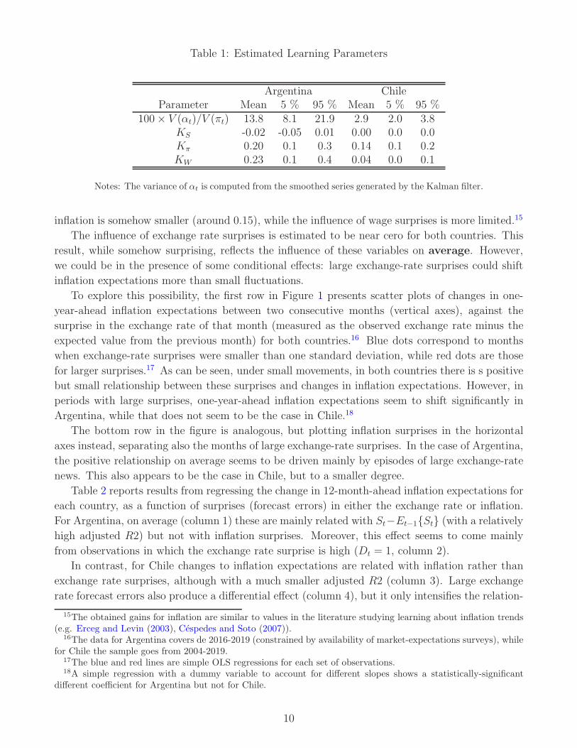
Table 1: Estimated Learning Parameters

Argentina ChileParameter Mean 5 % 95 % Mean 5 % 95 %

100× V (αt)/V (πt) 13.8 8.1 21.9 2.9 2.0 3.8KS -0.02 -0.05 0.01 0.00 0.0 0.0Kπ 0.20 0.1 0.3 0.14 0.1 0.2KW 0.23 0.1 0.4 0.04 0.0 0.1

Notes: The variance of αt is computed from the smoothed series generated by the Kalman filter.

inflation is somehow smaller (around 0.15), while the influence of wage surprises is more limited.15

The influence of exchange rate surprises is estimated to be near cero for both countries. This

result, while somehow surprising, reflects the influence of these variables on average. However,

we could be in the presence of some conditional effects: large exchange-rate surprises could shift

inflation expectations more than small fluctuations.

To explore this possibility, the first row in Figure 1 presents scatter plots of changes in one-

year-ahead inflation expectations between two consecutive months (vertical axes), against the

surprise in the exchange rate of that month (measured as the observed exchange rate minus the

expected value from the previous month) for both countries.16 Blue dots correspond to months

when exchange-rate surprises were smaller than one standard deviation, while red dots are those

for larger surprises.17 As can be seen, under small movements, in both countries there is s positive

but small relationship between these surprises and changes in inflation expectations. However, in

periods with large surprises, one-year-ahead inflation expectations seem to shift significantly in

Argentina, while that does not seem to be the case in Chile.18

The bottom row in the figure is analogous, but plotting inflation surprises in the horizontal

axes instead, separating also the months of large exchange-rate surprises. In the case of Argentina,

the positive relationship on average seems to be driven mainly by episodes of large exchange-rate

news. This also appears to be the case in Chile, but to a smaller degree.

Table 2 reports results from regressing the change in 12-month-ahead inflation expectations for

each country, as a function of surprises (forecast errors) in either the exchange rate or inflation.

For Argentina, on average (column 1) these are mainly related with St−Et−1St (with a relatively

high adjusted R2) but not with inflation surprises. Moreover, this effect seems to come mainly

from observations in which the exchange rate surprise is high (Dt = 1, column 2).

In contrast, for Chile changes to inflation expectations are related with inflation rather than

exchange rate surprises, although with a much smaller adjusted R2 (column 3). Large exchange

rate forecast errors also produce a differential effect (column 4), but it only intensifies the relation-

15The obtained gains for inflation are similar to values in the literature studying learning about inflation trends(e.g. Erceg and Levin (2003), Cespedes and Soto (2007)).

16The data for Argentina covers de 2016-2019 (constrained by availability of market-expectations surveys), whilefor Chile the sample goes from 2004-2019.

17The blue and red lines are simple OLS regressions for each set of observations.18A simple regression with a dummy variable to account for different slopes shows a statistically-significant

different coefficient for Argentina but not for Chile.

10

Figure 1: Inflation Expectations vs. Exchange Rate and Inflation Surprises

-20 -10 0 10 20 30 40-2

0

2

4

6

8

10

-10 -5 0 5 10 15 20-1

-0.8

-0.6

-0.4

-0.2

0

0.2

0.4

0.6

0.8

1

-1 0 1 2 3 4-2

0

2

4

6

8

10

-1 -0.5 0 0.5 1-1

-0.8

-0.6

-0.4

-0.2

0

0.2

0.4

0.6

0.8

1

Note: The vertical axes are always the change in 12-month-ahead inflation expectations between month t

and t−1, expressed in percentage points (Etπt,t+12−Et−1πt−1,t−1+12). In the top row of graphs, the

horizontal axes display the difference between the observed nominal exchange rate at t and the market

forecast from month t−1, expressed in percentage change St−Et−1St. In the bottom row, the horizontal

axes are the difference between the observed inflation at t and the market forecast from period t − 1,

expressed in percentage change (πt − Et−1πt).

11

Table 2: Changes in inflation expectation and surprises

Argentina ChileSt − Et−1St 0.16*** 0.04 0.00 0.01πt − Et−1πt -0.01 -0.14 0.15*** 0.08**

(St − Et−1St)Dt 0.14*** -0.02(πt − Et−1πt)Dt 0.30 0.65**

Const. 0.06 -0.05 0.00 0.01Nobs 42 42 219 219R2-adj 0.70 0.62 0.05 0.14

Notes: The dependent variable is the change in 12-month-ahead inflation expectations between

month t and t− 1. The regressors are one-month-ahead forecast errors. The variable Dt equals

one if the exchange rate forecast error is higher than one standard deviation. ∗∗∗ and ∗∗ denotes

significance at 99% and 95% level, respectively, computed with HAC standard errors.

ship with inflation surprises. Overall, this evidence suggests that in the country with more limited

credibility, medium-term inflation expectations are significantly affected by large movements in

the exchange rate, while this relationship is less evident in the country enjoying a relatively higher

degree of anchoring.

Given these results, in what follows we will use two calibrations for limited credibility: one

with KS = 0, Kπ = KW = 0.2 and another where KS = Kπ = KW = 0.2.19 The first tries to

capture lack of credibility under normal-size shocks, while the latter is meant to capture situations

where exchange rate volatility further hinders credibility.

2.9 Alternative policy rules

Our exploration of alternative simple rules considers the following:

1. Interest-rate rule:

(Rt

R

)=

(Rt−1

R

)ρR[(πt

π

)απ

(yHtyHt−1

)αy]1−ρR

eMPt , (6)

where eMPt is an i.i.d. policy shock.20 This is a Taylor-type rule, that we calibrate ρR = 0.8,

απ = 1.5, αy = 0.05, following the estimates for Chile in Medina and Soto (2007).

2. Monetary rule:

∆Mt =Mt

Mt−1

= π, (7)

i.e. money grows at the long-run inflation rate.

19The matrix Φ is calibrated using the posterior mean for the case of Argentina (the first column in the tableshown in Appendix B).

20We use this shock to understand the monetary transmission mechanism.

12

3. Nominal-exchange-rate rule:

πSt = πS, (8)

so that the exchange rate grows at the long-run depreciation rate. Given our calibration

(πS = 1) this is equivalent to an exchange rate peg.

3 Comparing Instruments under Rational Expectations

We begin by analyzing the model under rational expectations. We first explore the monetary

transmission mechanism by studying the responses of a policy shock under the interest-rate rule

in equation (6), displayed in Figure 2. As in most New-Keynesian models of small and open

economies, a negative shock to the Taylor rule leads to a rise in consumption, investment and

GDP. At the same time, due to the interest rate parity, the nominal exchange rate depreciates.

Both the rise in aggregate demand and the nominal depreciation increase inflation and, due to

price stickiness, the real exchange rate also depreciates. We can also see that the path of inflation

forecasts just equals that of actual inflation starting from period one (i.e. there is perfect foresight

under rational expectations ).

Next, we turn to the impact of a shock that increases the external interest rate by one standard

deviation, displayed in Figure 3.21 The solid-blue line depicts the responses under the interest-rate

rule. This shock contracts consumption and investment. The former is reduced through both a

negative wealth effect (as the country is a net-foreign borrower) and an intertemporal substitution

effect (savings become relatively more attractive). It also reduces investment by increasing the

real interest rate. This drop in aggregate absorption leads to a real depreciation, which in turn

raises aggregate inflation (by the increase in the domestic price of foreign goods), outweighing the

influence of aggregate-demand contraction. Also, due to sticky prices and wages, the required real

depreciation is achieved by an increase in the nominal exchange rate. The trade balance improves

driven by the drop in domestic absorption (which reduces imports), while quantities exported are

no sensitive to the real depreciation.

As inflation increases, the policy rate rises guided by the rule in equation (6). However, this

increase is relatively mild, for the rise in inflation is not as large. Moreover, the rising policy

rate somehow dampens the exchange rate dynamics, and therefore its impact on inflation. Along

the same lines, money balance also falls, reflecting both the fall in consumption and (to a lower

degree) the interest rate increase.

The dashed-red lines in Figure 3 are the dynamics under the constant-money-growth rule

in equation (7). Qualitatively, the contractionary effects of the shock on absorption also occur

under this configuration. The exchange rate and inflation dynamics also go in the same direction.

But the responses are quantitatively different. To understand the intuition, we can think of the

responses under the interest-rate rule as a proxy of what would happen, ceteris paribus, if the

policy rate remained constant. In such a case, money demand would fall due to the contraction in

consumption. In a configuration with a constant-money-growth rule, the interest rates must fall to

21As described in Appendix A, this is calibrated by estimating an AR(1) model to the sum of the LIBOR rateplus the J. P. Morgan EMBI Index for Argentina. The shock represents an increase of 280 annualized basis pointsin the cost of foreign borrowing.

13

Figure 2: Policy Shock under Interest-Rate Rule. Rational Expectations

5 10 15 200

0.1

0.2

0.3

5 10 15 200

0.1

0.2

0.3

5 10 15 20-0.5

0

0.5

1

5 10 15 20-0.1

-0.05

0

0.05

5 10 15 200

0.5

1

5 10 15 200.5

1

1.5

5 10 15 20-0.1

0

0.1

0.2

5 10 15 20-0.1

0

0.1

0.2

5 10 15 20-0.4

-0.2

0

0.2

5 10 15 20-0.4

-0.2

0

0.2

5 10 15 20-0.5

0

0.5

5 10 15 20-0.4

-0.2

0

0.2

Notes: Each panel displays the impulse responses to the following variables: GDP (yh), consumption (c), investment

(i), the trade-balance-to-output ratio (tbt/yHt ), real exchange rate (rer), nominal exchange rate (S), inflation (π),

expected inflation (Etπt+1), policy rate (R), ex-ante real rate (Rt − Etπt+1), money demand growth (∆M1)

and the shock hitting the economy. Al variables are measured in percentage deviations relative to the steady state,

except for tbt/yHt which is expressed as percentage points relative to its steady state value.

14

Figure 3: External-Interest-Rate Shock with Alternative Instruments. Rational Expectations

5 10 15 20-2

-1

0

1

5 10 15 20-2

-1

0

5 10 15 20-10

-5

0

5 10 15 200

0.5

1

1.5

5 10 15 200

2

4

6

5 10 15 200

2

4

6

5 10 15 20-0.5

0

0.5

5 10 15 20-0.5

0

0.5

5 10 15 20-0.5

0

0.5

1

5 10 15 20-1

0

1

2

5 10 15 20-4

-2

0

2

5 10 15 200

0.5

1

Notes: The solid-blue line is the version with an interest-rate rule, the dashed-red lines use a money-growth rule,

and the dashed-dotted-black lines correspond to the exchange-rate peg. See the description in Figure 2 for variables’

definitions.

15

clear the money market. This in turn leads to a larger nominal depreciation,22 which puts upward

pressure on inflation. At the same time, the real depreciation is larger (the addition nominal

depreciation outweighs the higher inflation).

Given the path for the real interest rate, relative to the previous case the effect on consumption

and investment is milder, which in turn implies an initially larger output expansion. Overall, we

can see that a money-growth rule produces more limited activity effects, at the cost of higher

inflation and a larger nominal and real depreciation.

Finally, the exchange-rate peg, equation (8), corresponds to the dashed-dotted-black line in

Figure 3. The contraction in absorption is larger in this case: by eliminating the nominal-exchange-

rate effect, domestic rates and spreads experience a larger increase.23 In contrast, under this

instrument inflation falls: as the nominal-exchange-rate channel disappears, prices are only driven

by aggregate demand (as in a closed economy).

To further summarize the desirability of each alternative, we ranked them using two metrics.

The first one is conditional welfare. For each model, with a given rule, we compute,24

W = ERW0

∞∑

t=0

βtU (ct, ht)

,

i.e. the expected welfare conditional on having experienced a positive shock to RW in period 0,

starting from the steady state, computed by a second-order approximation. We also compute the

consumption compensation that makes households indifferent between alternatives. In particular,

for a given reference equilibrium r and an alternative a, we define Λ implicitly such that

ERW0

∞∑

t=0

βtU (cat , hat )

= ERW

0

∞∑

t=0

βtU ((1− Λ)crt , hrt )

,

i.e. the percentage of per-period consumption that households would be willing to sacrifice to

live in the alternative a, relative to the equilibrium in r (if Λ < 0 agents prefer the situation a).

Finally, we also compare alternatives according to a loss function that weights equally deviations

of output and inflation from steady state, i.e.

L = ERW0

∞∑

t=0

βt[(yt)

2 + (πt)2],

which is frequently used to characterize policy under an inflation-targeting framework (e.g. Svens-

son, 2010).

22By the interest rate parity, the exchange rate increases here due to both the direct effect of an increase in theforeign-interest rate and the fall in domestic rate.

23The interest rate parity under a peg forces the policy rate to replicate the expected path of the external rate.24Notice that although the utility function in section 2 included also real money balances, we omit them here.

We choose to do so because we consider this to be just a shortcut to model money demand, and not an relevantcharacteristic to rank outcomes. Additionally, expectations here are taken according to the equilibrium distribu-tion. In cases where agents are adaptive learners, this implies that the welfare criteria is taking into account theimplications of such learning for equilibrium outcomes (i.e. using the actual instead of the perceived law of motionto form expectations).

16

Table 3 summarizes these comparisons, including also the volatilities of output, inflation and

the real exchange rate to complement the analysis. The equivalence measure Λ is computed relative

to the interest rate rule. In terms of welfare, the reduction in the volatility of aggregate demand

brought about by the money rule improves welfare (even though inflation is more volatile). But

the gain is relatively small: agents are willing to give up less than 0.2% of consumption to live in

a world with a money rule. In contrast, welfare is the lowest under a peg, and the consumption

equivalent is more than five times higher than in the comparison between money and interest-rate

rules. If we focus instead on the loss function, the M rule is slightly preferred to the R rule, while

under the S rule the loss is much higher.

Table 3: Volatilities, Welfare and Loss Function:Alternative Rules under Rational Expectations

Relative Volatilities Welfare RelativeRules yHt πt rert Λ LossM vs R 0.98 1.38 1.15 -0.17 -0.02S vs R 1.16 1.44 0.54 0.94 0.22

Notes: The first three columns show the ratio of standard deviations of output, inflation and

the real exchange rate, under either the M or the S rule, relative to those under the R rule. Λ

is computed using the model with R rule as the reference in each case, expressed in percentage

points. The last columns report the loss function under either the M or the S rule, minus that

under the R rule (a positive number indicates R is preferred).

Overall, under rational expectations, the identified trade-off between the responses of inflation

and output while comparing theM and the R rules is resolved slightly in favor of the money-growth

rule with either ranking criteria. In contrast, the peg is clearly dominated.

4 Comparing Instruments under Limited Credibility

We now turn to the analysis under limited credibility. We proceed in three steps. First, we study

how the monetary transmission mechanism changes in the presence of both limited-credibility

configurations (which recall differ on the assumption about KS). Second, we compare how the

propagation after the external-interest-rate shock differs depending on the expectations setup,

assuming that policy follows an interest rate rule. Finally, we compare the three alternative rules

under both deviations from rational expectations.

4.1 Transmission of Shocks Under Learning

In Figure 4 the effects of a negative policy shock in equation (6) under rational expectations are

displayed in solid-blue lines, while the case of limited credibility with KS = 0 is displayed with

dashed-red lines. The shock implies a larger and more persistent impact on activity when agents

use the empirical model to forecast inflation, while prices are relatively less sensitive.

To understand this result consider the real rate that affects consumption and investment deci-

sions: Rt−Etπt+1. Under rational expectations, agents understand that the expansion generated

17

by a more dovish policy stance will increase inflation in the future. Thus, the relevant real rate

drops more than the nominal rate.

Figure 4: Policy Shock under Interest-Rate Rule. Rational Expectations vs. ImperfectCredibility

5 10 15 20-0.2

0

0.2

0.4

5 10 15 20-0.2

0

0.2

0.4

5 10 15 20-1

0

1

2

5 10 15 20-0.2

-0.1

0

0.1

5 10 15 20-0.5

0

0.5

1

5 10 15 200

0.5

1

1.5

5 10 15 20-0.1

0

0.1

0.2

5 10 15 20-0.1

0

0.1

0.2

5 10 15 20-0.4

-0.2

0

0.2

5 10 15 20-0.4

-0.2

0

0.2

5 10 15 20-0.5

0

0.5

1

5 10 15 20-0.4

-0.2

0

0.2

Notes: The solid-blue line is the version under rational expectations, the dashed-red line is the version of imperfect

credibility with KS = 0, and the dashed-dotted-black lines use KS = 0.2. See the description in Figure 2 for

variables’ definitions.

If, instead, expectations incorporate inflation surprises only slowly, ceteris paribus the real

rate remains at a low level for a longer period (as inflation expectations are more persistent).

This leads to a somehow larger expansion in domestic absorption. However, inflation does not

increase despite the higher path for aggregate demand because the forward-looking channel of the

Phillips curve is muted under this type of learning. Thus, prices are less sensitive to the shock

on impact, although more persistent than under rational expectations. We can also see that the

path of expected inflation doesn’t match that of realized inflation: instead of perfect foresight as

in rational expectations, past inflation shapes agents’ forecast.

A relevant corollary of this analysis is that, to achieve a given desired effect on inflation,

the policy rate needs to move by more (and for a longer period) if expectations are not fully

rational. This in turn generally leads to larger sacrifice ratios during disinflations, as documented

18

by Gibbs and Kulish (2017), and it is the main channel emphasized by the learning literature in

closed-economy setups (e.g. Eusepi et al. (2020)).

In the same figure, dashed-dotted-black lines show the case with KS = 0.2. Here inflation

expectations rise by more than when they are rational, with a one-period delay because the

inference about αt is predetermined on impact (recall the assumption discussed in Section 2.8).

Under this setup, a more expansionary policy stance leads to more inflation than “intended”

if KS > 0. As we will analyze next, this implies that the relevant policy trade-off could be

exacerbated following a contractionary shock that induces a depreciation.

Figure 5 compares the responses after an external interest rate increase, still assuming the

interest-rate-policy rule. As can be seen, if learning features KS = 0 (dashed-red lines) the effects

on consumption and investment are not as different in the initial quarters; for the impact comes

mainly through a real channel and it is less related to inflation expectations. Afterward the con-

traction is larger and more persistent, explained by the reaction of the policy rate. As can be seen,

inflation and its expectation are marginally larger initially (due to the autoregressive component

of the expectation model, Φ in equation (3)) but, crucially, they remain above the steady-state

for a longer period (generated by the impact of actual inflation in long-run expectations, αt in the

forecasting model). This implies a relatively more persistent policy-rate path (as implied by the

R rule), explaining the additional contraction in activity.

If instead expectations are affected by the exchange-rate surprises (dashed-dotted-black lines

show the case with KS > 0) dynamics are further altered. Inflation increases by more as long-run

expectations shift, and GDP also falls by more. This effect in activity comes from two channels.

The policy rule dictates a more contractionary path, leading to a larger fall in demand. At the

same time, the real depreciation is smaller in this case (inflation increases by more, and the rise

in domestic rates dampens the nominal depreciation), limiting any expenditure-switching effect.

Therefore, if the exchange-rate jump feeds into expectations (as the evidence presented in section

2.8 seems to suggest under limited credibility) policy will face a worse trade-off between inflation

and activity after such this shock. In fact, in terms of conditional welfare and the loss function,

Table 4 shows that limited credibility is indeed costly.

Table 4: Volatilities, Welfare and Loss Function:Rational Expectations vs Limited Credibility under R Rule

Relative Volatilities Welfare RelativeAlternatives yHt πt rert Λ Loss

LC, KS = 0 vs RE 1.05 1.06 0.86 0.13 0.83LC, KS = 0.2 vs RE 1.23 1.79 0.54 0.76 0.51

Notes: All alternatives use the R rule, and the reference is the rational-

expectations version. For more details, see notes in Table 3.

4.2 Alternative Policy Rules

Figure 6 compares the three policy alternatives in the context of limited credibility if KS = 0.

Qualitatively, the differences between these rules are analogous to the analysis in Section 3: a

19

Figure 5: External-Interest-Rate Shock under Interest-Rate Rule. Rational Expectations vs.Imperfect Credibility

5 10 15 20-2

-1

0

1

5 10 15 20-2

-1

0

5 10 15 20-10

-5

0

5 10 15 200

0.5

1

1.5

5 10 15 200

2

4

6

5 10 15 200

2

4

6

5 10 15 20-0.5

0

0.5

1

5 10 15 20-0.5

0

0.5

1

5 10 15 20-0.2

0

0.2

0.4

5 10 15 20-0.4

-0.2

0

0.2

5 10 15 20-1

-0.5

0

0.5

5 10 15 200

0.5

1

Notes: The solid-blue line is the version under rational expectations, the dashed-red line is the version of imperfect

credibility with KS = 0, and the dashed-dotted-black lines use KS = 0.2. See the description in Figure 2 for

variables’ definitions.

learning mechanism where only past values of inflation shape long-term expectations does not

seem to alter the intuitive differences between the three alternatives.

Quantitatively the differences are exacerbated in this setup, due to two complementary effects.

First, as previously identified, the presence of adaptive learners induces a more persistent response

in nominal variables. Thus, the part of the trade-off between instruments related to inflation

dynamics gets amplified under lack of credibility. In particular, a constant-money-growth rule

implies somehow higher and more persistent inflation and depreciation than with an interest-rate

rule.

The differences in the behavior of interest rates are also amplified, yielding larger discrepancies

between the three cases in terms of real variables. The contraction is milder with the constant

money-growth rule while it is even larger under a peg. Overall, if long-term expectations are only

affected by past values of inflation, the trade-off between interest-rate and money-based rules is

20

Figure 6: External-Interest-Rate Shock with Alternative Instruments. Imperfect Credibility withKS = 0.

5 10 15 20-4

-2

0

2

5 10 15 20-3

-2

-1

0

5 10 15 20-20

-10

0

10

5 10 15 20-1

0

1

2

5 10 15 200

2

4

6

5 10 15 200

2

4

6

5 10 15 20-0.5

0

0.5

5 10 15 20-0.5

0

0.5

5 10 15 20-0.5

0

0.5

1

5 10 15 20-1

0

1

5 10 15 20-4

-2

0

2

5 10 15 200

0.5

1

Notes: All responses correspond to the learning model with KS = 0, the solid-blue lines are from the version with

an interest-rate rule, the dashed-red lines use a money-growth rule, and dashed-dotted-black lines correspond to

the exchange-rate peg. See the description in Figure 2 for variables’ definitions.

more pronounced. Moreover, the contractionary effects under a peg are larger under imperfect

credibility, and it is still not obvious that inflation volatility is reduced.

The top panel of Table 5 presents the comparison in welfare and loss-function terms. Relative

to the results under rational expectations in Table 3, here the M rule leave agents marginally

worse off under both metrics. Differences with the peg are similar in welfare terms, but not in

terms of the loss function.

If expectations are also affected by exchange rate dynamics (Figure 7), the comparison between

rules is different. Under both money and interest-rate rules, inflation expectations are higher due

to this additional learning channel. But here the real-rate path is relatively more contractionary

with the M than with the R rule. As a results, the activity path is much similar under these

two policies. Therefore the dampening effect in activity brought about by the money-growth rule

is less significant. In contrast, the peak in inflation is still almost twice as large than with the

21

Table 5: Volatilities, Welfare and Loss Function:Alternative Rules under Limited Credibility

Relative Volatilities Welfare RelativeRules yHt πt rert Λ Loss

Limited Credibility, KS = 0M vs R 1.03 1.26 1.13 0.23 0.02S vs R 1.32 1.10 0.74 0.95 0.53

Limited Credibility, KS = 0.2M vs R 1.03 1.23 1.12 0.19 0.06S vs R 1.06 0.48 0.70 0.46 0.12

Notes: See the description in Table 3 for details.

interest rate rule.

The exchange rate peg induces similar dynamics regardless of the type of learning assumed.

However, ifKS > 0 the difference in activity with the other rules is somehow smaller. Additionally,

the path of inflation is now less volatile under the peg than with the other alternatives. These

results are confirmed in the bottom panel of Table 5. The comparison between R and M rules is

similar in both learning structures, although aggregate volatility is higher. The difference is that

here, in relative terms the welfare cost of a peg is halved.

Overall, the trade-off in choosing the policy instrument seems to change depending on whether

exchange-rate movements directly influence expectations or not. If they do, the potential for

money-based rules to dampen the contraction is more limited. Moreover, there might be some

advantages in limiting exchange-rate fluctuations that are not present if learning is influenced by

past inflation only. This stresses the role to account for the role that exchange rate might have in

limited credibility environments.

5 Sensitivity Analysis

In this section, we compare the same policy rules under several model modifications: financial

frictions in the form of an endogenous foreign-financing spread; habits at the good-level further

limiting the expenditure-switching channel; a domestic banking sector that yields a richer structure

for monetary aggregates; a fraction of households with restricted access to financial markets; and a

final version combining all of them. To save space, the analysis focuses only on volatilities, welfare

and loss-function comparisons; while the impulse responses analogous to Figures 3, 6 and 7 for

each case are included in Appendix C.

5.1 Financial Frictions

A large literature highlights the role of financial frictions in propagating shocks in emerging coun-

tries, particularly those exposed to the liability dollarization phenomena.25 We explore how our

results change if these concerns are present. To keep the model as simple as possible, we follow

25See, for instance, the survey by Mendoza and Rojas (2019).

22

Figure 7: External-Interest-Rate Shock with Alternative Instruments. Imperfect Credibility withKS = 0.2.

5 10 15 20-4

-2

0

2

5 10 15 20-3

-2

-1

0

5 10 15 20-15

-10

-5

0

5 10 15 200

0.5

1

1.5

5 10 15 200

2

4

6

5 10 15 20-5

0

5

5 10 15 20-0.5

0

0.5

1

5 10 15 20-0.5

0

0.5

1

5 10 15 20-1

0

1

5 10 15 20-2

-1

0

1

5 10 15 20-4

-2

0

2

5 10 15 200

0.5

1

Notes: All responses correspond to the learning model with KS = 0.2, The solid-blue line are the version with an

interest-rate rule, the dashed-red lines use a money-growth rule, and dashed-dotted-black lines correspond to the

exchange-rate peg. See the description in Figure 2 for variables’ definitions.

Garcıa-Cicco and Garcıa-Schmidt (2020) and make the external premium elastic to the ratio of

foreign debt to GDP. In particular, we change the external-interest-rate equation (2) to:

R∗

t = RWt exp

φ

(−rertb

∗

t

pHt yHt

+ b

). (9)

Furthermore, we double the value of φ from 0.001 to 0.002.

To understand the effect of such a change, notice that in the baseline model the shock to

RWt increases the debt ratio in (9); either because debt rises, activity falls, a real depreciation

is induced, or a combination of them. As a consequence, under financial frictions, the shock is

relatively more contractionary. If also φ increases, a larger depreciation is generated and inflation

23

further increases.26 This first line in Table 6 contrast this new setup under the R rule and

the baseline model with the same rule, both under rational expectations. As can be seen, this

modification rises volatility in the economy by around 50%, both for real and nominal variables.

Moreover, the conditional welfare cost of suffering a negative shock to RW in a world with this

endogenous premium is significantly higher relative to the baseline.

Table 6: Volatilities, Welfare and Loss Function:Alternative Rules with Financial Frictions


Rational Expectations

R vs Base R 1.54 1.48 1.55 5.50 0.38M vs R 1.02 1.49 1.21 0.39 0.02S vs R 1.01 1.39 0.51 -0.67 0.16



Notes: the first line compares the R rule under rational expectation in this alternative, using

as reference the Baseline model under rational expectation with the R rule. The other lines

compare each policy alternative with the R rule under this particular model, and each panel

differs only by the expectation-formation assumption, as in Table 3.

Given the presence of financial frictions, we investigate the relative merits of each policy rule,

considering each expectation-formation setup. Focusing first on rational expectations, we can see

that theM rule further increases volatility relative to the R rule, particularly for inflation and the

real exchange rate. Thus, the advantages of theM rule identified in the baseline model are limited

if financial frictions are relevant. In contrast, by limiting the real depreciation that would otherwise

affect the endogenous premium, the peg has some advantages under rational expectations, and in

terms of conditional welfare is even preferred to the other rules.27

Under limited credibility, the R rule seems to dominate the other alternatives in terms of both

conditional welfare and the loss function. The relative merits of M rule are also diminished under

learning, while the cost of a peg (which under learning is no longer preferred to the R rule) is

milder, particularly if KS = 0.2. Therefore, the potential advantages of reducing exchange rate

volatility identified with the baseline model are strengthened if financial frictions are present.

5.2 Good-Level Habits

The expenditure-switching channel in isolation would imply an expansion after any shock that

induces a real depreciation, as it implies (ceteris paribus) an improvement in the trade balance.

26If we just change the premium to (9) but maintain φ = 0.001, the differences are small between models.27This does not necessarily imply that the peg is the optimal rule under financial frictions, it just desirable among

the three alternatives considered here. The optimal-policy analysis is beyond the scope of this paper.

24

As the evidence for emerging countries points to a contractionary effect of increases in foreign

interest rates (e.g. Uribe and Yue, 2006), it seems appropriate to investigate the robustness of

the result if the expenditure-switching channel is further limited.28 To that end, we modify the

assumption regarding habit formation in the model: we eliminate habits at the total-consumption

level as in the baseline, and instead set the aggregation of final goods in equation (1) to,

yCwt =

[ω1/η

(xHt − φCx

H,at−1

)1−1/η

+ (1− ω)1/η(xFt − φCx

F,at−1

)1−1/η] η

η−1

. (10)

where xH,at and xF,at denote aggregate values of xHt and xFt and respectively (i.e. external habits).

This alternative, inspired by the deep-habits setup of Ravn et al. (2012), limits the expenditure-

switching channel because a given change in relative prices affects the relative demand for H and

F only gradually. Table 7 reports the comparison in this case. Relative to the baseline under the

R rule and rational expectations, the volatility of the economy is slightly greater, due to a mildly

larger contraction originated by the negative shock.

Table 7: Volatilities, Welfare and Loss Function:Alternative Rules with Good-level Habits



R vs Base R 1.01 1.05 1.00 0.26 0.99M vs R 0.98 1.35 1.14 -0.21 -0.02S vs R 1.14 1.37 0.56 1.39 0.20




The rules comparison under rational expectations is similar than in the baseline, with the dif-

ferences marginally exacerbated: as the dampening impact of the deprecation on activity induced

by expenditure-switching is reduced, both the potential benefits of a peg and the extra exchange-

rate volatility induced by the M rule are less important in terms of welfare. Once we allow for

limited credibility, both results analyzed in the baseline are maintained: the R rule is preferred

to both alternatives (with only a small difference relative to the M rule), and there might be

potential benefits to limit exchange-rate fluctuations if KS > 0.

28The dominant-currency pricing assumption already contributes to this, by making exports insensitive to thereal exchange rate. However, the expenditure-switching channel is still active in the substitution between H andF goods domestically.

25

5.3 Domestic Banks

It might be argued that the baseline setup is somehow simple to study the M rule, as a variety of

monetary aggregates exist in real life. To include this possibility, we add a banking sector to the

model. We assume households derive utility from real holdings of both cash Mt/Pt and deposits

Dt/Pt. In addition, the purchase of capital goods now requires to finance a fraction αLK with loans

(Lt) from banks: Lt ≥ αKLQtkt.

Banks operate a technology characterized by a cost function ξBt Ψ(Dt, Lt), where ξBt is an

exogenous variable and Ψ is increasing, convex and linear homogeneous. Following Edwards and

Vegh (1997), this implies that loans and deposits are complements (e.g. due to economies of scale

in monitoring borrowers). This sector is competitive and banks are required to hold reserves τtper unit of deposit, remunerated at a rate Rτ

t .

Dividends for the representative bank at t + 1 are

ΩBt+1 =

(RL

t Lt − Lt+1

)+Dt+1(1− τt+1)−

(RD

t −Rτt τt

)Dt − ξBt+1Ψ(Dt+1, Lt+1).

The goal is to maximize the net-present-value of dividends (i.e. Et

∑∞

h=0 χt,t+hΩBt+h

). The

optimality conditions can be written in terms of two relevant spreads:

Rt −RDt = (Rt −Rτ

t ) τt +RtξBt ΨD,t, (11)

RLt − RD

t = (Rt − Rτt ) τt +Rtξ

Bt (ΨL,t +ΨD,t) , (12)

Spreads arise for two different reasons. First, in the presence of required reserves, both spreads are

positive as long as the policy rate is higher than that at which reserves are remunerated (usually

the empirically relevant case). From this channel, a policy rate hike, ceteris paribus, increases

both spreads. The second is related to marginal costs. In equation (11), the second term on the

right-hand side can be shown to be increasing in the deposits-to-loans ratio. In equation (12), the

second term on the right-hand side is also increasing in the deposits-to-loans ratio (given that the

calibration assumes that deposits are larger than loans in steady state). Thus, from this channel

also, an increase in the policy rate widens both spreads.29

In this setup, we assume that the M rule targets nominal base-money growth, with MBt =

Mt + τtDt. The functional forms and calibration are detailed in Appendix A, and results are

displayed in Table 8. Compared with the baseline under the R rule and rational expectations,

this variant displays relatively milder volatility. However, in welfare terms agents are worse-off,

for inefficiency is generated by the presence of spreads to finance investment.

Conditional on living in a world with banks, the comparison between the different rules under

alternative expectations setups is similar to that in the baseline model. If anything, the cost of a

peg is somehow smaller with banks, particularly in the case in which exchange rate surprises feed

into long-term expectations (KS = 0.2).

29Notice that this banking system operates fully in domestic-currency assets. While banks could be exposedto a currency-mismatch problem, evidence suggests that this phenomenon has significantly decreased over time(for instance, Tobal (2018) presents evidence for Latin America and the Caribean). Moreover potential liabilitydollarization issue could be relevant for the non-banking sector as well, which is addressed in the financial-frictionssensitivity analysis previously presented.

26

Table 8: Volatilities, Welfare and Loss Function:Alternative Rules with Banks



R vs Base R 0.95 0.96 0.94 2.24 1.06M vs R 0.99 1.37 1.15 -0.13 -0.02S vs R 1.14 1.39 0.55 0.78 0.18




5.4 Restricted Access to Financial Markets

Arguments against using the interest rate as the main policy instrument are many times related

to the fact that, if a large part of the population does not have access to financial markets, the

interest rate is not a relevant price for most agents in the economy; e.g. Berg et al. (2010), Andrle

et al. (2013). To consider this possibility, we assume the presence of two types of households:

Constrained (of mass Γ) and Unconstrained (of mass 1− Γ); as in, for instance, Galı et al. (2007)

or Colciago (2011). The former just consumes its labor income, i.e.30

PtcCt =Wtht,

and demands money to pay for a fraction of their consumption purchases (equal to the ratio of

money to GDP in the baseline model). Changes in the policy rate will only affect consumption

decisions for these agents to the extent that an equilibrium change in labor and/or wages is

triggered. Instead, unconstrained households solve the same problem as the representative agents

in the baseline. Therefore, in equilibrium,

ct = ΓcCt + (1− Γ)cUt .

The rest of the model is analogous to the baseline. We calibrate Γ = 0.7. Results are displayed in

Table 9.31

Relative to the baseline model under rational expectations and the R rule, the world-interest-

rate shock generates a similar volatility in activity and inflation, but a higher real-exchange-rate

30Given the preference setup featuring no wealth effect in labour supply, both types of households will optimallywork the same amount of hours; i.e. hC

t = hUt = ht. Moreover, we assume labor productivity is the same for both

types of households. Therefore, wages are also the same for both of them.31In performing welfare comparisons with this model, we compute three consumption-equivalent measures: two

of them compare the utility for each type of agents (ΛC and ΛU ), while we also compare welfare obtained usingaggregate consumption (Λ) as a measure of “average” welfare costs.

27

Table 9: Volatilities, Welfare and Loss Function:Alternative Rules with Restricted Access to Financial Markets

Relative Volatilities Welfare RelativeAlternatives yHt πt rert Λ ΛU ΛC Loss


R vs Base R 0.99 1.03 1.12 0.24 – – 1.13R vs M 0.98 1.38 1.15 -0.39 -0.29 -0.99 0.050R vs S 1.16 1.44 0.54 1.73 1.75 2.68 -0.294

Limited Credibility, KS = 0R vs M 1.03 1.26 1.13 -0.04 -0.29 0.66 -0.031R vs S 1.32 1.10 0.74 3.96 5.46 1.71 0.905

Limited Credibility, KS = 0.2R vs M 1.03 1.23 1.12 0.10 0.07 0.52 0.047R vs S 1.06 0.48 0.70 1.01 1.07 1.09 0.202


variance. While not shown in the table, aggregate consumption is more volatile in this model, as

constrained agents cannot smooth the shock. This in turn explains the additional relative price

volatility. In contrast, investment is relatively less affected by the external shock in this setup, for

asset prices are determined by unrestricted consumption only (which is relatively less volatile).

Overall, both in welfare and loss-function terms, the average household is worse off living in a

word where a fraction of agents is cannot access financial markets.

Comparing alternative rules with constrained households, under rational expectations both

types of agents would prefer the money-based rule, particularly those that cannot access finan-

cial markets to smooth consumption. It is still the case (as in the baseline) that the M rule

induces higher inflation and relative-price volatility, while smoothing activity. In fact, the R rule

is marginally preferred according to the loss function. In contrast, the welfare cost of a peg under

rational expectations is much larger in this model: the additional contraction is particularly costly

for constrained households.

If limited credibility is in place, results change in the same direction as in the baseline. It is

worth highlighting that the average welfare cost of a peg is much larger if KS = 0 (in the baseline

was similar to rational expectations), but this comes mainly from unconstrained households. The

welfare-cost differences also appear with theM rule: if KS = 0 constrained households now dislike

this rule, while the comparison is the same for unconstrained ones.

Finally, if KS = 0.2, results are similar to those obtained in the baseline. Both households

would prefer the R rule, while the relative cost of a peg is milder under this expectation assumption.

5.5 Full model

Finally, we construct a model that features all the characteristics previously introduced to study

the sensitivity of the result; labeled the Full model. Most characteristics can be easily combined

in the model, as they refer to a different aspect of the economy. The only caveat worth mentioning

is that we assume that constrained households only use cash, while only unconstrained agents use

28

bank deposits. Results are reported in Table 10. Relative to the baseline, the volatility in all three

variables reported is larger and the welfare cost of combining all features is significant.

Table 10: Volatilities, Welfare and Loss Function:Alternative Rules in the Full Model

Relative Volatilities Welfare RelativeAlternatives yHt πt rert Λ ΛU ΛC Loss


R vs Base R 1.40 1.66 1.55 7.47 0.45R vs M 1.02 1.49 1.21 0.00 -0.03 -0.13 -0.059R vs S 1.01 1.39 0.51 0.51 1.01 0.36 0.249

Limited Credibility, KS = 0R vs M 1.06 1.30 1.15 0.35 -0.51 2.29 -0.035R vs S 1.25 1.12 0.69 3.46 5.36 1.09 1.222

Limited Credibility, KS = 0.2R vs M 1.02 1.26 1.12 -0.09 -0.56 1.02 -0.014R vs S 1.03 0.52 0.70 0.61 0.78 0.91 0.201


The rules comparison yields similar results under rational expectations. We can also see that

the disagreement in terms of welfare regarding the M rule is exacerbated in the full model under

learning. Instead, the relative merits of reducing exchange rate volatility if KS is appreciated by

both types of agents. Overall, none of the main results obtained under the baseline model are

refuted with these model modifications.

6 Conclusions

This paper presented a model-based analysis of the relevant trade-offs of alternative simple rules

for different monetary-policy instruments. The focus was on how these alternatives can help in

smoothing the impact of shocks to external-borrowing costs depending on the policy configuration.

Importantly, we explored how conclusions are altered in the presence of imperfect credibility,

captured by departing from rational expectations (using instead simple time-series models to

forecast inflation-related variables).

We documented that, qualitatively, there is a trade-off in choosing between a Taylor-type rule

for the interest rate vs. a constant-money-growth rule. In particular, limiting fluctuations in the

quantity of money insulates activity-related variables from the contractionary effects of the shock.

At the same time, the inflationary effects are magnified in a monetary targeting framework. Finally,

an exchange-rate peg induces a larger contraction in the economy, without necessarily creating an

improvement in the inflation front.

We also showed that these trade-offs are amplified in the presence of limited credibility if

the learning mechanism is mainly driven by past inflation observations (the channel generally

emphasized in the related literature). This is due to both a more persistent inflation process and

the different interest-rate behavior under this configuration.

29

Instead, if the exchange rate can directly influence medium- and long-term inflation expecta-

tions, the comparison among alternatives changes. In particular, the potential benefits of money-

growth rules are reduced, and there might be a role for limiting exchange rate volatility to prevent

large shifts in inflation expectations. Moreover, we presented evidence suggesting that this addi-

tional exchange-rate channel in the learning process could be empirically relevant in cases with

limited credibility.

While this exploration allows identifying relevant dimensions of the policy-instrument discus-

sion, it also suggests that further work is needed to provide a more detailed evaluation. On one

hand, a more thorough empirical analysis of the influence of exchange rate surprises in shaping

inflation expectations could shed light on the relevant channels contributing to inflation anchoring.

On the other, the rules analyzed here were relatively simple. One could also include other feedback

variables in the rules (the exchange rate in particular) or different parameters. A study of optimal

simple rules (from a welfare perspective) for a given instrument and a comparison between the

best rule for each instrument should be desirable.

Finally, we have also abstracted from the presence of money-demand shocks that could, a

priori, induce higher volatility under money-growth rules. In other words, the quote from former

the Bank of Canada governor Bouey, “We didn’t abandon monetary aggregates, they abandoned

us,” was not considered in the analysis performed; although it should be included in a more

complete quantitative assessment. We leave these considerations for future research.

References

Adler, G., Lama, R., and Medina, J. P. (2019). Foreign exchange intervention and inflation

targeting: The role of credibility. Journal of Economic Dynamics and Control, 106(C):1–36.

Agenor, P.-R. and Pereira da Silva, L. (2017). Cyclically adjusted provisions and financial stability.

Journal of Financial Stability, 28(C):143–162.

Aguirre, H., Burdisso, T., and Grillo, F. (2006). Towards an Estimation of Money Demand with

Forecasting Purposes: Argentina, 1993-2005. Ensayos Economicos, 1(45):7–44.

Andrle, M., Berg, A., Berkes, E. G., Portillo, R. A., Vlcek, J., and Morales, R. A. (2013). Money

Targeting in a Modern Forecasting and Policy Analysis System; an Application to Kenya. IMF

Working Papers 13/239.

Arias, A. and Kirchner, M. (2019). Shifting Inflation Expectations and Monetary Policy. Working

Papers Central Bank of Chile 829.

Berg, A., Unsal, F. D., and Portillo, R. A. (2010). On the Optimal Adherence to Money Targets in

a New-Keynesian Framework; An Application to Low-Income Countries. IMF Working Papers

10/134.

Burstein, A. and Gopinath, G. (2014). International Prices and Exchange Rates. In Gopinath,

G., Helpman, ., and Rogoff, K., editors, Handbook of International Economics, volume 4 of

Handbook of International Economics, pages 391–451. Elsevier.

30

Calvo, G. A. (2018). Fighting chronic inflation with interest rates: Cutting a hydra’s heads with

a swiss army knife? mimeo, Columbia University.

Calvo, G. A. and Vegh, C. A. (1994). Inflation Stabilization And Nominal Anchors. Contemporary

Economic Policy, 12(2):35–45.

Calvo, G. A. and Vegh, C. A. (1999). Inflation stabilization and b.o.p. crises in developing

countries. In Taylor, J. B. and Woodford, M., editors, Handbook of Macroeconomics, volume 1,

chapter 24, pages 1531–1614. Elsevier.

Carriere-Swallow, Y., Gruss, B., Magud, N. E., and Valencia, F. (2016). Monetary Policy Credi-

bility and Exchange Rate Pass-Through. IMF Working Papers 2016/240.

Carvalho, C., Eusepi, S., Moench, E., and Preston, B. (2020). Anchored inflation expectations.

CAMA Working Papers 2020-25.

Cogley, T., Matthes, C., and Sbordone, A. M. (2015). Optimized Taylor rules for disinflation when

agents are learning. Journal of Monetary Economics, 72(C):131–147.

Colciago, A. (2011). Rule-of-Thumb Consumers Meet Sticky Wages. Journal of Money, Credit

and Banking, 43:325–353.

Corsetti, G., Dedola, L., and Leduc, S. (2010). Optimal Monetary Policy in Open Economies. In

Friedman, B. and Woodford, M., editors, Handbook of Monetary Economics, volume 3, chap-

ter 16, pages 861–933.

Cespedes, L. F. and Soto, C. (2007). Credibility and Inflation Targeting in Chile. In Miskin,

Schmidt-Hebbel, and Loayza, editors, Monetary Policy under Inflation Targeting, volume 11,

chapter 14, pages 547–578.

De Paoli, B. (2009). Monetary policy and welfare in a small open economy. Journal of International

Economics, 77(1):11–22.

Devereux, M. B., Lane, P. R., and Xu, J. (2006). Exchange Rates and Monetary Policy in Emerging

Market Economies. Economic Journal, 116(511):478–506.

Edwards, S. and Vegh, C. A. (1997). Banks and macroeconomic disturbances under predetermined

exchange rates. Journal of Monetary Economics, 40(2):239–278.

Erceg, C. J. and Levin, A. T. (2003). Imperfect credibility and inflation persistence. Journal of

Monetary Economics, 50(4):915–944.

Eusepi, S., Giannoni, M., and Preston, B. (2020). On the Limits of Monetary Policy. Technical

report, mimeo, UT Austin.

Eusepi, S. and Preston, B. (2011). Expectations, Learning, and Business Cycle Fluctuations.

American Economic Review, 101(6):2844–2872.

31

Eusepi, S. and Preston, B. (2018a). Fiscal Foundations of Inflation: Imperfect Knowledge. Amer-

ican Economic Review, 108(9):2551–2589.

Eusepi, S. and Preston, B. (2018b). The Science of Monetary Policy: An Imperfect Knowledge

Perspective. Journal of Economic Literature, 56(1):3–59.

Evans, G. W. and Honkapohja, S. (2001). Learning and Expectations in Macroeconomics. Prince-

ton University Press.

Faia, E. (2008). Optimal monetary policy rules with labor market frictions. Journal of Economic

Dynamics and Control, 32(5):1600–1621.

Faia, E. and Monacelli, T. (2007). Optimal interest rate rules, asset prices, and credit frictions.

Journal of Economic Dynamics and Control, 31(10):3228–3254.

Faia, E. and Monacelli, T. (2008). Optimal Monetary Policy in a Small Open Economy with Home

Bias. Journal of Money, Credit and Banking, 40(4):721–750.

Galı, J., Lopez-Salido, J. D., and Valles, J. (2007). Understanding the Effects of Government

Spending on Consumption. Journal of the European Economic Association, 5(1):227–270.

Galı, J., Smets, F., and Wouters, R. (2012). Unemployment in an Estimated New Keynesian

Model. NBER Macroeconomics Annual, 26(1):329–360.

Garcıa-Cicco, J. and Garcıa-Schmidt, M. (2020). Revisiting the exchange rate pass through: A

general equilibrium perspective. Journal of International Economics, 127.

Garcıa-Cicco, J., Kirchner, M., and Justel, S. (2015). Domestic Financial Frictions and the Trans-

mission of Foreign Shocks in Chile. In Raddatz, Saravia, and Ventura, editors, Global Liquidity,

Spillovers to Emerging Markets and Policy Responses, volume 20, chapter 6, pages 159–222.

Gaspar, V., Smets, F., and Vestin, D. (2010). Inflation Expectations, Adaptive Learning and

Optimal Monetary Policy. In Friedman, B. M. andWoodford, M., editors, Handbook of Monetary

Economics, volume 3 of Handbook of Monetary Economics, chapter 19, pages 1055–1095.

Ghosh, A. R., Ostry, J. D., and Chamon, M. (2016). Two targets, two instruments: Monetary

and exchange rate policies in emerging market economies. Journal of International Money and

Finance, 60(C):172–196.

Gibbs, C. G. and Kulish, M. (2017). Disinflations in a model of imperfectly anchored expectations.

European Economic Review, 100(C):157–174.

Gopinath, G., Boz, E., Casas, C., Dıez, F. J., Gourinchas, P.-O., and Plagborg-Moller, M. (2020).

Dominant Currency Paradigm. American Economic Review, 110(3):677–719.

Lama, R. and Medina, J. P. (2011). Optimal Monetary Policy and Social Insurance in a Small

Open Economy. The B.E. Journal of Macroeconomics, 11(1):1–40.

32

Medina, J. P. and Soto, C. (2007). The Chilean Business Cycles Through the Lens of a Stochastic

General Equilibrium Model. Working Papers Central Bank of Chile 457.

Mendoza, E. G. and Rojas, E. (2019). Positive and Normative Implications of Liability Dollariza-

tion for Sudden Stops Models of Macroprudential Policy. IMF Economic Review, 67(1):174–214.

Ravn, M. O., Schmitt-Grohe, S., and Uribe, M. (2012). Consumption, government spending, and

the real exchange rate. Journal of Monetary Economics, 59(3):215–234.

Schmitt-Grohe, S. and Uribe, M. (2003). Closing small open economy models. Journal of Inter-

national Economics, 61(1):163–185.

Schmitt-Grohe, S. and Uribe, M. (2007). Optimal simple and implementable monetary and fiscal

rules. Journal of Monetary Economics, 54(6):1702–1725.

Svensson, L. E. (2010). Inflation Targeting. In Friedman, B. M. and Woodford, M., editors,

Handbook of Monetary Economics, volume 3 of Handbook of Monetary Economics, chapter 22,

pages 1237–1302.

Taylor, J. B. (2019). Inflation targeting in high inflation emerging economies: lessons about rules

and instruments. Journal of Applied Economics, 22(1):103–116.

Taylor, J. B. and Williams, J. C. (2010). Simple and Robust Rules for Monetary Policy. In Fried-

man, B. and Woodford, M., editors, Handbook of Monetary Economics, volume 3, chapter 15,

pages 829–859.

Tobal, M. (2018). Currency Mismatch in the Banking Sector in Latin America and the Caribbean.

International Journal of Central Banking, 14(1):317–364.

Uribe, M. and Yue, V. Z. (2006). Country spreads and emerging countries: Who drives whom?

Journal of International Economics, 69(1):6–36.

A Functional Forms and Calibration

In the sake of space, we present the calibration of the version that also includes banks. The

baseline model is obtained by simply setting RDt = RL

t = Rt, τt = 0 and ξBt = 0.

The utility function is set in a way that yields the following characteristics: (i) labor supply

has no wealth effect, (ii) the inter-temporal consumption trade-off is independent of labor and

liquidity related decisions, (iii) money and deposits demands have unitary elasticity with respect to

consumption and a parameter governing the elasticity for the relevant rates, and (iv) consumption,

money and deposits decisions are persistent. The first two characteristics are desirable to obtain

a negative effect in activity under interest rate shocks.32 The other conditions generate dynamics

32Otherwise, either the wealth effect on labor supply or the indirect effect of labor in the marginal utility ofconsumption may lead to expansionary effects after an interest rate increase.

33

for consumption, money and deposits decisions that are empirically plausible. The specification

is,

(ct)1−σ

1− σ− Ξh

t

(ht)1+ϕ

1 + ϕ+ ΞM

t

(mt)1− 1

σM

1− 1σM

+ ΞDt

(dt)1− 1

σD

1− 1σD

where ct, mt, dt denote habit-adjusted consumption as well as real cash and deposit.33 The utility

shifters (taken as given by individuals) Ξht , Ξ

Mt and ΞD

t are set to get the desired restrictions. In

particular:

− For labor we pick Ξht = ξh(ct − φCct−1)

−σ. This yields a labor supply given by:

wtmcWt = ξhhϕt

where ξh is a parameter. This approach follows Galı et al. (2012), who argue that this

externality in the supply of labor induces, in equilibrium, that labor-supply decisions are

independent from consumption, yielding at the same time separability in the utility.

− Similarly, for money and deposits we set Ξjt = (ξj)

1

σj−1(ct − φCct−1)

1

σj−σ

, for j = M,D,where ξj are parameters. This generates the following demands for money and deposits:

mt − φMmt−1 =(1− R−1

t

)−σM (ct − φcct−1) ξ

M ,

dt − φDdt−1 =

(1− RD

t

Rt

)−σD

(ct − φcct−1)ξD,

which yield the desired properties.

The capital-adjustment-cost function is set to

S

(itit−1

)=φI

2

(itit−1

− 1

)2

with φI > 0. The bank’s cost function is,

Ψ(D,L) = ψ0 + ψDD + ψLL− 2ψDL

√DL

following Agenor and Pereira da Silva (2017). The parameter ψDL determines the elasticity of the

spread with respect to the deposits-to-loans ratio, ψD and ψL are related with the steady-state

values of RL and RD, and ψ0 pins down the size of banking costs relative to the rest of the economy.

We use the following calibration strategy. We choose values for all parameters and exogenous

variables in the model, except for β, π∗, RW , ν, y∗, b, g, ξM , ξD, ψ0, ψD, ψL, σM , σD that are endoge-

nously determined to match the following steady-state values: CPI inflation (π), hours worked (h),

relative price of home goods (pH), the nominal interest rate (R), nominal depreciation (πS), the

trade-balance-to-output ratio (stb = tb/(pHyH)), the ratio of government expenditure to output

(sg = g/(pHyH)), the shares of money over GDP (sm = m/(pHyH)), the ratio of deposits to loans

33For a generic variable xt, habit adjusted is given by xt = xt−φXxat−1, with xa

t = xt in equilibrium. We furtherassume that, individually, households take xa

t as given (i.e. preferences exhibits external habits).

34

(sdl = d/l), the share of bank costs to GDP (sBcost = BcosttpHyH

), the lending and deposit rates (RL

and RD), and the elasticity of money and deposits demand with respect to the relevant rates (εM

and εD).

The calibrated values are shown in Table 11. Most macro-related parameters are calibrated

following the literature on estimated DSGE models for emerging countries (e.g. Medina and Soto,

2007, Garcıa-Cicco et al., 2015), and therefore are not discussed here. In terms of bank-related

parameters, we choose a lending-deposit spread of 6 annual percentage points (a.p.p.). The ratio

of deposits to loans is larger than one (similar to the average ratio in Argentina between 2017 and

2018), indicating a relatively underdeveloped financial market. The share of banks costs on GDP

is in line with the ratio of sectoral GDP of the financial sector in most Latin American countries.

The parameter ψDL is set to a relatively small value to have a modest volatility of the spread.

The elasticity of money and deposit demand follows the empirical literature for Latinamerica (e.g.

Aguirre et al., 2006).

Finally, the process for the external interest rate (which will be the main focus of the analysis)

is parametrized by fitting an AR(1) process to the sum of the LIBOR rate and the JPMorgan

EMBI Index for Argentina. The standard deviation of the shock represents an annualized value

of around 280 basis points in a quarter. In turn, the calibrated persistence implies a half-life of

almost 5 quarters.

35

Table 11: Calibrated parameters and targeted steady state values.

Parameter Description Valueσ Coef. of relative risk aversion 2ϕ Inverse Frisch elasticity of labor suppy 1φC Habit in consumption 0.6φM Habit in money demand 0.3φD Habit in deposits demand 0.3α Share of capital in production of H 0.33δ Capital depreciation 0.015φI Inv. adjustment cost 3αKL Share of capital financed by loans 0.5ω Share of home goods in consumption 0.7η Elast. of subst. between home and for. goods 0.5η∗ Foreign demand elasticity 0.2ǫ Elast. of subst. between varieties of goods 11ǫW Elast. of subst. between varieties of labor 11θ Calvo probability of no price adjustment 0.7θW Calvo probability of no wage adjustment 0.9ϑ Indexation to past inflation in prices 0.4ϑW Indexation to past inflation in wages 0.8φB Debt elasticity of foreign interest rate 0.001ψDL Elasticity of the spread to the deposit-to-loan ratio 0.01ρRW Autocorr. external interest rate 0.7σRW St.Dev. external interest rate shock 0.007

π Steady state inflation 1.031/4

h Steady state hours worked 1/3pH Steady state rel. price of home goods 1R Steady state domestic interest rate 1.061/4

πS Steady state exchange. rate growth 1stb Steady state trade-balance-to-GDP ratio 0.05sg Steady state government-consumption-to-GDP ratio 0.1sm Steady state inverse velocity of money 0.3sdl Steady state deposits-to-loans ratio 1.2sBcost Steady state of banking costs 0.01RD Deposit interest rate R×0.991/4

RL Lending interest rate R×1.051/4

τ Required reserves 0.15Rτ Interest rate on required reserves 1εM Money demand elasticity -1.5/4εD Deposits demand elasticity 1/4

36

B Learning Parameters

Table 12: Other Estimated Learning Parameters

Argentina ChileParameter Mean 5 % 95 % Mean 5 % 95 %

Φ1,1 0.039 -0.142 0.213 -0.321 -0.436 -0.204Φ1,2 0.306 -0.293 0.951 0.286 -0.521 1.072Φ1,3 0.015 -0.795 0.886 0.486 -0.748 1.683Φ2,1 0.042 -0.019 0.100 0.005 -0.004 0.013Φ2,2 0.532 0.341 0.710 0.215 0.143 0.287Φ2,3 -0.126 -0.418 0.141 0.033 -0.056 0.131Φ3,1 0.015 -0.033 0.063 0.003 -0.014 0.020Φ3,2 0.414 0.252 0.573 0.094 -0.082 0.262Φ3,3 0.083 -0.173 0.362 0.051 -0.162 0.279

37

C Sensitivity Analysis

Figure 8: Alternative Instruments with Financial Frictions. Rational Expectations.

5 10 15 20-4

-2

0

2

5 10 15 20-3

-2

-1

0

5 10 15 20-15

-10

-5

0

5 10 15 200.5

1

1.5

2

5 10 15 200

5

10

5 10 15 200

5

10

5 10 15 20-0.5

0

0.5

1

5 10 15 20-0.5

0

0.5

1

5 10 15 20-0.5

0

0.5

1

5 10 15 20-1

0

1

2

5 10 15 20-4

-2

0

2

5 10 15 200

0.5

1

38

Figure 9: Alternative Instruments with Financial Frictions. Imperfect Credibility with KS = 0.

5 10 15 20-4

-2

0

2

5 10 15 20-3

-2

-1

0

5 10 15 20-20

-10

0

10

5 10 15 200

1

2

3

5 10 15 200

5

10

5 10 15 200

5

10

5 10 15 20-0.5

0

0.5

1

5 10 15 20-0.5

0

0.5

1

5 10 15 20-0.5

0

0.5

1

5 10 15 20-1

0

1

5 10 15 20-4

-2

0

2

5 10 15 200

0.5

1

39

Figure 10: Alternative Instruments with Financial Frictions. Imperfect Credibility withKS = 0.2.

5 10 15 20-4

-2

0

2

5 10 15 20-3

-2

-1

0

5 10 15 20-15

-10

-5

0

5 10 15 200

1

2

5 10 15 200

2

4

6

5 10 15 200

5

10

5 10 15 20-0.5

0

0.5

1

5 10 15 20-0.5

0

0.5

1

5 10 15 20-1

0

1

5 10 15 20-2

-1

0

1

5 10 15 20-4

-2

0

2

5 10 15 200

0.5

1

40

Figure 11: Alternative Instruments with Good-level Habits. Rational Expectations.

5 10 15 20-2

-1

0

1

5 10 15 20-4

-2

0

5 10 15 20-10

-5

0

5 10 15 200

0.5

1

1.5

5 10 15 200

2

4

6

5 10 15 200

2

4

6

5 10 15 20-0.5

0

0.5

5 10 15 20-0.5

0

0.5

5 10 15 20-0.5

0

0.5

1

5 10 15 20-1

0

1

5 10 15 20-4

-2

0

2

5 10 15 200

0.5

1

41

Figure 12: Alternative Instruments with Good-level Habits. Imperfect Credibility with KS = 0.

5 10 15 20-4

-2

0

2

5 10 15 20-4

-2

0

5 10 15 20-20

-10

0

10

5 10 15 200

0.5

1

1.5

5 10 15 200

2

4

6

5 10 15 200

5

10

5 10 15 20-0.5

0

0.5

5 10 15 20-0.5

0

0.5

5 10 15 20-0.5

0

0.5

1

5 10 15 20-1

0

1

5 10 15 20-4

-2

0

2

5 10 15 200

0.5

1

42

Figure 13: Alternative Instruments with Good-level Habits. Imperfect Credibility with KS = 0.2.

5 10 15 20-3

-2

-1

0

5 10 15 20-4

-2

0

5 10 15 20-20

-10

0

10

5 10 15 200

0.5

1

1.5

5 10 15 200

2

4

6

5 10 15 200

2

4

6

5 10 15 20-0.5

0

0.5

1

5 10 15 20-0.5

0

0.5

1

5 10 15 20-1

0

1

5 10 15 20-2

-1

0

1

5 10 15 20-4

-2

0

2

5 10 15 200

0.5

1

43

Figure 14: Alternative Instruments with Banks. Rational Expectations.

5 10 15 20-2

-1

0

1

5 10 15 20-2

-1

0

5 10 15 20-10

-5

0

5 10 15 200

0.5

1

1.5

5 10 15 200

2

4

6

5 10 15 200

2

4

6

5 10 15 20-0.5

0

0.5

5 10 15 20-0.5

0

0.5

5 10 15 20-0.5

0

0.5

1

5 10 15 20-1

0

1

5 10 15 20-4

-2

0

2

5 10 15 200

0.5

1

44

Figure 15: Alternative Instruments with Banks. Imperfect Credibility with KS = 0.

5 10 15 20-4

-2

0

2

5 10 15 20-3

-2

-1

0

5 10 15 20-20

-10

0

10

5 10 15 200

0.5

1

1.5

5 10 15 200

2

4

6

5 10 15 200

5

10

5 10 15 20-0.5

0

0.5

5 10 15 20-0.5

0

0.5

5 10 15 20-0.5

0

0.5

1

5 10 15 20-0.5

0

0.5

1

5 10 15 20-4

-2

0

2

5 10 15 200

0.5

1

45

Figure 16: Alternative Instruments with Banks. Imperfect Credibility with KS = 0.2.

5 10 15 20-4

-2

0

2

5 10 15 20-3

-2

-1

0

5 10 15 20-15

-10

-5

0

5 10 15 200

0.5

1

1.5

5 10 15 200

2

4

6

5 10 15 200

2

4

6

5 10 15 20-0.5

0

0.5

1

5 10 15 20-0.5

0

0.5

1

5 10 15 20-1

0

1

5 10 15 20-2

-1

0

1

5 10 15 20-4

-2

0

2

5 10 15 200

0.5

1

46

Figure 17: Alternative Instruments with Constrained Agents. Rational Expectations.

5 10 15 20-4

-2

0

2

5 10 15 20-4

-2

0

2

5 10 15 20-10

-5

0

5 10 15 200

0.5

1

1.5

5 10 15 200

2

4

6

5 10 15 200

5

10

5 10 15 20-0.5

0

0.5

5 10 15 20-0.5

0

0.5

5 10 15 20-0.5

0

0.5

1

5 10 15 20-1

0

1

2

5 10 15 20-4

-2

0

2

5 10 15 200

0.5

1

47

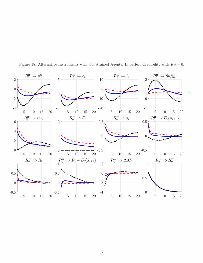
Figure 18: Alternative Instruments with Constrained Agents. Imperfect Credibility with KS = 0.

5 10 15 20-4

-2

0

2

5 10 15 20-5

0

5

5 10 15 20-20

-10

0

10

5 10 15 20-1

0

1

2

5 10 15 200

2

4

6

5 10 15 200

5

10

5 10 15 20-0.5

0

0.5

5 10 15 20-0.5

0

0.5

5 10 15 20-0.5

0

0.5

1

5 10 15 20-0.5

0

0.5

1

5 10 15 20-4

-2

0

2

5 10 15 200

0.5

1

48

Figure 19: Alternative Instruments with Constrained Agents. Imperfect Credibility withKS = 0.2.

5 10 15 20-4

-2

0

2

5 10 15 20-4

-2

0

5 10 15 20-20

-10

0

10

5 10 15 200

1

2

5 10 15 200

2

4

6

5 10 15 200

2

4

6

5 10 15 20-0.5

0

0.5

1

5 10 15 20-0.5

0

0.5

1

5 10 15 20-0.5

0

0.5

1

5 10 15 20-2

-1

0

1

5 10 15 20-4

-2

0

2

5 10 15 200

0.5

1

49

Figure 20: Alternative Instruments In Full Model. Rational Expectations.

5 10 15 20-4

-2

0

2

5 10 15 20-4

-2

0

5 10 15 20-20

-10

0

10

5 10 15 200

1

2

5 10 15 200

5

10

5 10 15 200

5

10

5 10 15 20-0.5

0

0.5

1

5 10 15 20-0.5

0

0.5

1

5 10 15 20-1

0

1

5 10 15 20-2

0

2

5 10 15 20-2

-1

0

1

5 10 15 200

0.5

1

50

Figure 21: Alternative Instruments In Full Model. Imperfect Credibility with KS = 0.

5 10 15 20-4

-2

0

2

5 10 15 20-5

0

5

5 10 15 20-20

-10

0

10

5 10 15 20-2

0

2

4

5 10 15 200

5

10

5 10 15 200

5

10

5 10 15 20-0.5

0

0.5

1

5 10 15 20-0.5

0

0.5

1

5 10 15 20-0.5

0

0.5

1

5 10 15 20-1

0

1

5 10 15 20-2

-1

0

1

5 10 15 200

0.5

1

51

Figure 22: Alternative Instruments In Full Model. Imperfect Credibility with KS = 0.2.

5 10 15 20-4

-2

0

2

5 10 15 20-4

-2

0

5 10 15 20-20

-10

0

10

5 10 15 200

1

2

5 10 15 200

2

4

6

5 10 15 200

5

10

5 10 15 20-0.5

0

0.5

1

5 10 15 20-0.5

0

0.5

1

5 10 15 20-2

-1

0

1

5 10 15 20-4

-2

0

2

5 10 15 20-2

-1

0

1

5 10 15 200

0.5

1

52

working paper n 91 | 2021 - bcra

Documents