working paper no. 159 - centre for development economics
TRANSCRIPT

CDE August, 2007
The Transfer Paradox in a One-Sector Overlapping Generations Model
Partha Sen Email: [email protected]
Department of Economics Delhi School of Economics
Delhi
&
Emily T. Cremers Email: [email protected]
National University of Singapore
Working Paper No. 159
Centre for Development Economics
Department of Economics, Delhi School of Economics
The Transfer Paradox in a One-Sector Overlapping Generations Model
Partha Sen Delhi School of Economics
Emily T. Cremers National University of Singapore
Abstract: This paper examines the effects of international income transfers on welfare and capital accumulation in a one-sector overlapping generations model. It is shown that a strong form of the transfer paradox-- in which the donor country experiences a welfare gain while the recipient country experiences a welfare loss—may occur both in and out of steady state. In addition, it is shown that a weak form of the transfer paradox—where either the donor or recipient (but not both) experience paradoxical welfare effects—may characterize all segments of the transition path not already characterized by the strong transfer paradox. The results are explained by the effects of transfers on world capital accumulation and the world interest rate, which imply secondary intertemporal welfare effects large enough to dominate the initial effects of the income transfer.
Key Words: Transfer problem, transfer paradox, dynamics, one-sector overlapping generations model
JEL Classification: F11, F35, F43, O19, O41 Correspondence to: Emily Cremers, Dept. of Economics, National University of Singapore, SINGAPORE 117570 Phone: (65) 6874-6832 Fax: (65) 6775-2646 Email: [email protected]
1
In this paper we examine the effects of an international income transfer in
a one-sector overlapping generations model. This adds to an extensive but
dated literature that examines the welfare effects of such transfers in a static
trade environment and also to a smaller, more recent literature that reconsiders
the consequences of transfers in a growth setting. Despite the emphasis on
dynamics found in the latter more closely related research, the literature has yet
to definitively pin down the effects of permanent transfers both in and out of
steady state equilibrium. This paper does just that, and in the process
demonstrates that versions of the transfer paradox—most generally recognized
as a situation in which the donor benefits from a transfer at the expense of the
recipient-- may arise both in the steady state and also at all dates comprising the
transition to that steady state. As will be shown, these welfare effects emerge as
a direct consequence of the transfer’s effects on world capital accumulation and
the intertemporal terms of trade.
In our two-country model, residents of the donor and recipient countries
are distinguished only by differences in their intertemporal discount rate, which
implies differences in the national propensities to save. Capital is assumed to be
perfectly mobile across these two countries so that a common world capital-labor
ratio and interest rate prevail at every date. The transfer under consideration is
both fixed in size and permanent; that is, an equal amount will be transferred
from the donor to the recipient country in each and every period. Because the
transfer alters savings in both countries, it is responsible for changes in the world
capital accumulation path. Thus, in addition to the direct effect of the transfer on
2

welfare of the donor and recipient countries, there are indirect effects that arise to
reflect the status of each country in the international credit market (ie, as a
borrower or lender) and also the effect of the transfer on the the world interest
rate in each period. The transfer is `paradoxical’ when these indirect effects are
both opposite in sign and larger in magnitude than the direct effects.
Our main theoretical findings are the following. When the initial steady
state is at the golden rule, the transition path can be characterized by both strong
and weak forms of the transfer paradox: in the former, both countries experience
a paradoxical welfare effect whereas, in the latter, only one of the two countries
is paradoxically affected by the transfer. More precisely, we identify a single
sufficient condition under which there is a weak transfer paradox in the short-run
followed by a strong transfer paradox in the long-run. When the initial steady
state is away from the golden rule, a strong transfer paradox is still possible in
the steady state, but dynamic (in)efficiency increases support for the weak
version of the paradox.
Our results concerning the transfer paradox are noteworthy on three
accounts. First, our steady state findings lend clarity to an existing literature that
incorporates permanent transfers into the one-sector overlapping generations
model so as to determine the long run welfare effects for the donor and recipient
countries. Galor and Polemarchakis (1987) argue that the transfer paradox is
possible both at and away from the golden rule steady state.1 However,
1 Galor and Polemarchakis (1987) also claim that, away from the golden rule, a transfer may be Pareto-improving. Both claims are said to be consistent with market stability. Unfortunately, all of these claims are brought to question by a technical oversight that is described in our footnote 2. Our steady state results revisit each of these claims and we are therefore indebted to the earlier analysis.
3
Haaparanta (1989) correctly identified an oversight in this analysis2 and
subsequently argued that the results concerning the paradox were only valid
when the initial steady state is dynamically inefficient. Tan (1998) later argued
that a steady state transfer paradox does not occur in the one-sector overlapping
generations model when transfers are made specifically from rich to poor
countries, where a rich country is defined as that which has the higher level of
per capita savings.3 This claim also contradicts Galor and Polemarchakis, who
did not specify a particular ranking of savings levels across countries. As it
stands, the perspective of the literature is thus skeptical towards the possibility of
a transfer paradox in a `sensible’ dynamic model of international transfers. Our
paper demonstrates that the skepticism is entirely unfounded.4 We reconsider
the conclusions of Galor and Polemarchakis and demonstrate their validity after
the oversight noted by Haaparanta is corrected.5 Also, we show that a transfer
from a high saving country to a low saving country is entirely compatible with a
steady state transfer paradox, in reversal of Tan. Overall, we build a case for
revising the dynamic literature’s perspective towards the transfer problem; in the
2 Specifically, Galor and Polemarchakis inadvertently equate national savings to domestic investment for each country when deriving their welfare expressions despite having made the assumption of international capital mobility. 3 To be less brief, but more accurate, Tan’s claim that the paradox does not arise requires first that the difference between the capital-labor ratio of the donor and recipient not be too large. However, in this setting, the capital-labor ratios of the two countries must be equal in equilibrium, which implies that Tan’s requirement is in fact always satisfied. 4 The analysis presented in Haaparanta (1989) was concerned with the effects of temporary, rather than permanent, transfers. And, as already noted, the conclusions of Tan (1998) are derived without acknowledging the role of international capital mobility on steady state capital-labor ratios. With these shortcomings, it is not clear that Galor and Polemarchakis (1987) has been invalidated. 5 In a recent paper, Yanagihara (2006) also demonstrates that corrected versions of the welfare expressions used by Galor and Polemarchakis cannot be signed under dynamic efficiency, which therefore leaves room for a transfer paradox. However, that paper neither derives a sufficient condition for the occurrence of a transfer paradox, nor considers out of steady state behavior, as we do in subsequent sections.
4

one-sector overlapping generations model there is a possibility of a steady state
transfer paradox both at and away from the golden rule.
A further comparison with the conclusions drawn from the earlier static
modeling of transfers reveals the second noteworthy aspect of our findings. In
the static literature, it was widely established that a transfer paradox cannot
occur under market stability except in the presence of a distortion, or
alternatively, a bystander to the transfer (see, for example, Bhagwati and Brecher
(1982), Bhagwati, Brecher and Hatta (1985), Gale (1974), Bhagwati, Brecher and
Hatta (1983), Yano (1983)). This conclusion stands in stark contrast to our own,
where the transfer paradox can be a robust feature of a dynamic, general
equilibrium, even when instability, distortions and bystanders are excluded. The
key to understanding this theoretical turnabout lies in the identification of the
effects of transfers on world savings and investment. In basic terms, transfer-
induced changes in world capital accumulation can introduce hitherto
unrecognized supply-side effects that intensify movements in the (intertemporal)
terms of trade. Therefore, if the earlier literature is seen to undermine the
general theoretical relevance of the transfer paradox, then this paper clarifies that
it is primarily the adherence to a static modeling framework that makes it so. In
other words, the needed revisal in perspective towards the transfer paradox goes
beyond the confines of the dynamic literature discussed above.
A final theoretical contribution follows from the inclusion of the welfare
effects of transfers on generations living in the transition to the steady state. In
so doing, our analysis is more comprehensive than Galor and Polemarchakis
5

(1987), Tan (1998) and Yanagihara (2006), who focus only one the steady state
effects of permanent transfers, and Haaparanta (1989), who is primarily
concerned with short- and long-run effects of a one-shot, temporary transfer. By
including an analysis of the transitional periods we are able to preempt the notion
that steady state implications are somehow `special’ and may belie non-
paradoxical, short-run welfare effects. Again, the occurrence of a transfer
paradox in our model is not a peculiarity of the steady state, but rather is shown
to be a potentially pervasive feature of a world growth path.
Section 2 describes the environment and world equilibrium absent
international transfers. Section 3 introduces the transfers when the initial steady
state is at the golden rule capital-labor ratio and separately describes the welfare
effects for generations born in the initial period of the transfer, the transitional
periods, and also the steady state. Section 4 summarizes these results and
identifies a sufficient condition for the occurrence of a transfer paradox at all
dates along the equilibrium path. This condition is then reinterpreted as a
restriction on the elasticity of factor substitution. Section 5 considers the impact
that dynamic (in)efficiency may have on prospects for the transfer paradox.
Specifically, we show that the steady state transfer paradox cannot be ruled out,
although the transfer may lead to welfare deterioration in both countries when the
initial steady state is dynamically efficient and a mutual welfare improvement
when it is dynamically inefficient. A parametric example in Section 6
demonstrates the transfer paradox under the assumption of dynamic efficiency.
The concluding remarks are then made in Section 7.
6

2. Two-country model with capital mobility
There are two countries in the world economy, a donor, , and recipient, D
R , of an international income transfer. Let denote the number of individuals
that are born in each of the two countries at date t . Each member of generation
lives for two periods and is `young’ at time and `old’ at date . Both
populations grow equally and exogenously, according to
tL
t t 1t +
1(1 )t tL n L −= + 0n >, ,
where the members of generation 0 are assumed to live only during the initial
period, . Thus, at each date , both countries are populated by two
overlapping generations comprised of the young members of generation and
the old members of generation
0L
1t = 1t ≥
t
1t − .
Each individual is endowed with one unit of labor when young; thus,
also denotes the endowment of labor in each country at date . In addition, at
, the initial old in each of the two countries possess equal amounts of the
initial capital stock. Let denote the initial ratio of capital to labor available for
production in the first period. It is assumed that capital does not depreciate and
that the stock of capital can grow via production. The capital-labor ratio in each
country during each of the subsequent periods includes, therefore, both old and
new capital.
tL t
1t =
1k
Labor is immobile across the two countries and is hired by firms in a
national, competitive labor market. Capital, however, is internationally mobile
and is priced in a global, competitive market. Firms comprise the demand side of
7

the market for capital, whereas individuals in both countries supply capital
acquired via savings and investment.
2.1 Production and factor markets
The two countries utilize a common technology in their production of the
world’s only output. This technology is represented by a linearly homogenous
production function. In per capita terms, production at time in country is given
by
t j
( )jtf k , where is the input of capital per worker and denotes the intensive
form of the production function. For all , it is assumed that ,
, and . Furthermore, it is assumed that
jtk f
0jtk > ( ) 0j
tf k >
( ) 0jtf k′ > ( ) 0j
tf k′′ <0
lim ( ) 0k
f k→
= ,
and . 0
lim ( )k
f k→
′ = ∞ lim ( ) 0k
f k→∞
′ =
Let j and respectively denote the date t payment per unit of capital
and labor service in country . Firms demand capital and labor from individuals
so as to maximize profits. That is, is chosen so as to equate the respective
marginal productivities of capital and labor to their factor payments:
and , for
trj
tw
j
jtk
( )j jt tr f k′= ( ) '( )j j j
t t tw f k k f k= − jt , .j D R=
2.2 Consumption and savings The residents of the two countries, always equal in number, have
preferences that are represented by well-behaved utility functions, ,
which are defined over youthful and old age consumption, denoted and
, ,ju j D R=
jtc 1
jtd +
respectively for members of generation . Labor income earned by each young t
8
individual is divided between immediate consumption expenditures and savings,
the latter of which is used to finance consumption when old. Thus the
optimization problem for each member of generation t in country is to maximize
subject to budget constraints in the respective periods of life,
and , where denotes individual savings and
j
1( , )j j jt tu c d +
j jt tc s w+ = j
tj
ts1 1j j
t td ρ+ += jts 1
jtρ + is the
gross return on date savings. The solution to these problems can be
represented by the savings functions where . In
addition, it is assumed that . The initial old, living only at date 1, purchase
consumption goods using the proceeds from renting their capital to firms and
then selling it to the young of generation 2.
t
1( , )t , ,j j j jt ts s w j D Rρ += = 0j
ws >
0jsρ >
6 For all generations other than the
initial old, the optimal savings function implies a corresponding indirect utility
function 1( , )j j jt tV w ρ + . As is well-known, the envelope theorem implies that
and jwV u= j
cj j j
dV s uρ = ; thus, the indirect utility function is increasing in both its
arguments.
2.3 Equilibrium
The global capital market equates, in per capita terms, the aggregate
savings of each young generation with investment; that is, with the capital stock
to be made available for production in the subsequent period. Let and ts 1tk +
respectively denote per capita savings at time t and the world capital-labor ratio
at time . In the absence of depreciation, the return on savings is given by 1t +
16 As will become apparent below, 1 1
j jd kρ= .
9
1 1jt rρ + = + 1
jt+
1t
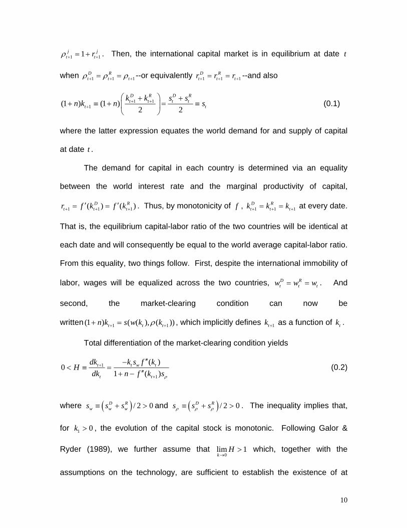
. Then, the international capital market is in equilibrium at date t
when 1 1D Rt tρ ρ ρ+ += = + 1--or equivalently 1 1
D Rt t tr r r+ += = + --and also
1 11(1 ) (1 )
2 2
D R D Rt t t t
tk k s s
n k n s+ ++
⎛ ⎞+ ++ ≡ + = ≡⎜ ⎟
⎝ ⎠t
1 )Rt+ 1
(0.1)
where the latter expression equates the world demand for and supply of capital
at date t .
The demand for capital in each country is determined via an equality
between the world interest rate and the marginal productivity of capital,
. Thus, by monotonicity of , 1 1( ) (Dt tr f k f k+ +′ ′= = f 1 1
D Rt t tk k k+ += = +
t
1t
at every date.
That is, the equilibrium capital-labor ratio of the two countries will be identical at
each date and will consequently be equal to the world average capital-labor ratio.
From this equality, two things follow. First, despite the international immobility of
labor, wages will be equalized across the two countries, . And
second, the market-clearing condition can now be
written
D Rt tw w w= =
1(1 ) ( ( ), ( ))t tn k s w k kρ++ = + , which implicitly defines 1tk + as a function of . tk
Total differentiation of the market-clearing condition yields
1
1
( )0
1 (t t w t
t t
dk k s f kH
dk n f k s) ρ
+
+
′′−< ≡ =
′′+ − (0.2)
where and ( ) / 2 0D R
w w ws s s≡ + > ( ) / 2 0D Rs s sρ ρ ρ≡ + > . The inequality implies that,
for , the evolution of the capital stock is monotonic. Following Galor &
Ryder (1989), we further assume that which, together with the
assumptions on the technology, are sufficient to establish the existence of at
1 0k >
0lim 1k
H→
>
10
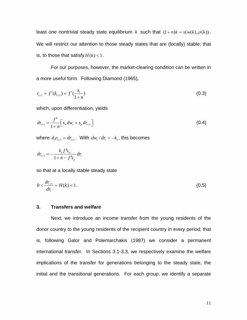
least one nontrivial steady state equilibrium such that (1k ) ( ( ), ( ))n k s w k kρ+ = .
We will restrict our attention to those steady states that are (locally) stable; that
is, to those that satisfy . ( ) 1H k <
For our purposes, however, the market-clearing condition can be written in
a more useful form. Following Diamond (1965),
1 1( ) (1
tt t
sr f k f
n+ +′ ′= =+
) (0.3)
which, upon differentiation, yields
1 1t w tfdr s dw s dr
n ρ+
′′⎡= +⎣+ 1t+ ⎤⎦
1tr
(0.4)
where 1td dρ + = + t. With /t tdw dr k= − , this becomes
1 1t w
t tk f s
dr drn f sρ
+
′′= −
′′+ −
so that at a locally stable steady state
10 (t
t
drH k
dr+< = <) 1. (0.5)
3. Transfers and welfare Next, we introduce an income transfer from the young residents of the
donor country to the young residents of the recipient country in every period; that
is, following Galor and Polemarchakis (1987) we consider a permanent
international transfer. In Sections 3.1-3.3, we respectively examine the welfare
implications of the transfer for generations belonging to the steady state, the
initial and the transitional generations. For each group, we identify a separate
11
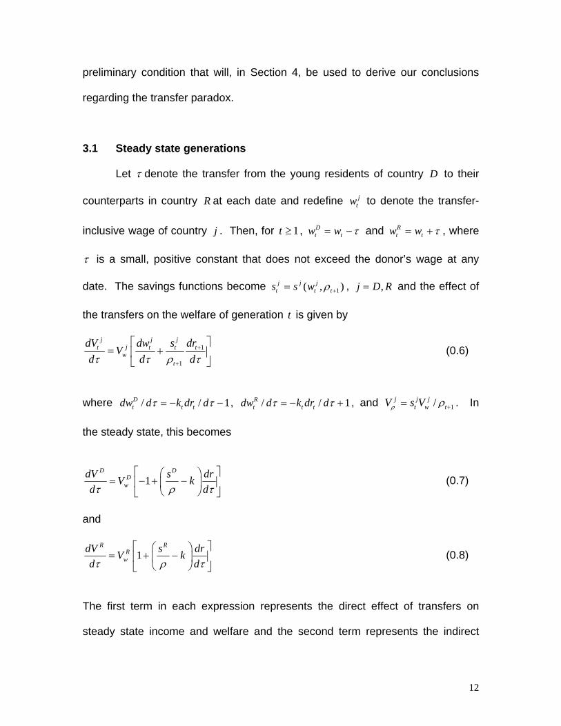
preliminary condition that will, in Section 4, be used to derive our conclusions
regarding the transfer paradox.
3.1 Steady state generations Let τ denote the transfer from the young residents of country to their
counterparts in country
D
R at each date and redefine to denote the transfer-
inclusive wage of country
jtw
j . Then, for , 1t ≥ Dt tw w τ= − and R
t tw w τ= + , where
τ is a small, positive constant that does not exceed the donor’s wage at any
date. The savings functions become , 1( , )j j jt ts s w ρ += t ,j D R= and the effect of
the transfers on the welfare of generation t is given by
1
1
j j jjt t t
wt
dV dw s drV
d d dt
τ τ ρ τ+
+
⎡ ⎤= +⎢
⎣ ⎦⎥
Dt t tdw d k dr d
(0.6)
where / / 1τ τ= − − / / 1Rt t tdw d k dr dτ τ, = − + , and 1/j j j
t w tV s Vρ ρ += . In
the steady state, this becomes
1D D
Dw
dV s drV kd dτ ρ τ
⎡ ⎤⎛ ⎞= − + −⎢ ⎜ ⎟
⎝ ⎠⎣ ⎦⎥ (0.7)
and
1R R
Rw
dV s drV kd dτ ρ τ
⎡ ⎤⎛ ⎞= + −⎢ ⎜ ⎟
⎝ ⎠⎣ ⎦⎥ (0.8)
The first term in each expression represents the direct effect of transfers on
steady state income and welfare and the second term represents the indirect
12

effects of the transfer that are channeled through the changes in the
intertemporal terms of trade.
Differentiating (0.3) now gives
( )
( )1 1 2 1
D Rw wt w
t t
f s sk f sdr dr d
n f s n f sρ ρ
τ+
′′ −′′= − −
′′+ − ′′+ −. (0.9)
( )D R
w ws s− is positive or negative as the donor or recipient has the respectively
higher propensity to save from wages. In the steady state this becomes
( )( )2 1
D Rw w
w
f s sdrd n f s kf sρτ
′′− −=
′′ ′′+ − + (0.10)
The stability condition implies that the denominator is positive, and hence
( )sgn sgn D Rw wdr d s sτ = − . Thus, the steady state interest rate is increased
(decreased) by a transfer when the donor has a greater (lesser) propensity to
save from wages than does the recipient. This is because such a transfer
decreases (increases) the world supply of savings and also therefore world
steady state capital accumulation.
To begin, we assume that 1 nρ = + ; that is, that the steady state is that
associated with the golden rule.7 There are two immediate implications. First,
using (0.1), it is straightforward to demonstrate that sgn sgnD RdV d dV dτ τ= − . In
other words, at the golden rule, if the transfer improves welfare of the donor then
it will necessarily worsen the welfare of the recipient. Second, since ,
(0.7) can be written
/(1 )k s n= +
7 This (temporary) assumption is analytically convenient and facilitates a comparison of our results with those in the existing literature. We consider steady states away from the golden rule in Section 5.
13

11
2
D DD
wdV s s drVd d
R
τ ρ τ⎡ ⎤⎛ ⎞−
= − +⎢ ⎥⎜ ⎟⎝ ⎠⎣ ⎦
. (0.11)
Clearly, if ( ) (sgn sgn )D R D
w ws s s s− = − R , then (0.11) shows that the intertemporal
welfare effect is always positive in the donor country.8 Also then, the
intertemporal welfare effect is always negative in the recipient country. More
particularly, regardless of the ranking of savings and savings propensities across
countries, the intertemporal terms of trade effect always changes in favor of the
transfer paradox.
How can this be explained? For insight, note that the market-clearing
condition (0.1) implies ( ) ( )/(1 ) /(1 )D Rs n k s n k+ − = − + − ; the net foreign
investment of the high-saving country will be equal in magnitude to, and of
opposite sign from, the low-saving country. If, for example, the donor country
has the higher average savings, it will be a net lender in the international capital
market, whereas the recipient will be a net borrower. Under the same
assumption, however, (0.10) implies 0dr dτ > . In this case, the positive welfare
effect described by (0.11) is derived from the fact that the international lender is
better off when there is an increase in the interest rate. Simultaneously, the
recipient country, being an international borrower, will be worse off as a result of
the increasing interest rate. If, on the other hand, the donor is the low saving
country, it will then be the international borrower but this time (0.10) implies
0dr dτ < . The positive effect on welfare reflects that the international borrower 8 The assumption that ( ) ( )sgn sgnD R D
w ws s s s− = − R is valid in the case of log-linear utility functions,
for example.
14

benefits from a reduction in the interest rate. And, the recipient, being the
international lender, experiences a decline in welfare as a result of the lower
interest rate.
For the intertemporal terms of trade to move by an amount that is
sufficient to generate the transfer paradox we must find conditions under which
1 12
D Rs s drdρ
⎛ ⎞−>⎜ ⎟
⎝ ⎠ τ. (0.12)
Let ε denote the elasticity of substitution so that . Then,
substitution into (0.2) and (0.10) respectively implies that
1( )wr kffε −′′= −
wwrksH
f s wrsρε=
+
and
12 1
D Rw w
w
s sdr Hd k s Hτ
⎛ ⎞− ⎛= ⎜ ⎟⎜ −⎝ ⎠⎝ ⎠
⎞⎟ (0.13)
Using the latter expression in (0.12), we are able to identify a sufficient condition
under which the effects of the transfer on steady state welfare are paradoxical
from the perspective of both the donor and recipient countries.
Proposition 1: Suppose the initial steady state is at the golden rule. If
1
2 2
D RD Rw w
w ws ss sH ss ss
−⎡ ⎤⎛ ⎞⎛ ⎞ −−
> +⎢ ⎜⎜ ⎟⎢ ⎥⎝ ⎠⎝ ⎠⎣ ⎦
⎥⎟ , then steady state welfare in the donor
country is improved by the transfer and steady state welfare in the recipient
country is worsened.
15

3.2 Initial young and old In the initial period, there is a fixed endowment of capital; consequently,
regardless of the transfer, 1 1 0dw dr= = . Thus, the initial old of both countries are
unaffected by the transfer and the initial effects fall upon generation 1. With
, 1 0dr = 1Ddw dτ= − , 1
Rdw dτ= and (0.9) gives
( )
( )22
2
( )
2 1 ( )
D Rw wf k s sdr
d n f k sρτ
′′− −=
′′+ − (0.14)
Consider first the effects of the transfer on the initial young in the donor country.
Under the stability assumption, ( )2sgn D Rw wdr d s sτ = − ; thus, the effect of the
transfer on the interest rate at 2t = is positive when the donor has the higher
savings propensity and negative otherwise.
The effect on the net wage, however, is always negative: .
Thus, from the version of (0.6), if the donor has the lower savings
propensity then it is immediate that the welfare of generation 1 is reduced
( ) by the transfer. Hence, there can be no transfer paradox from the
perspective of the initial young in the donor country. Otherwise, if the donor has
the higher savings propensity, then an increase in the interest rate works against
the negative direct effect of the transfer, and the overall welfare effect is
ambiguous.
1 / 1Ddw dτ = − < 0
1t =
1 0DdV <
16
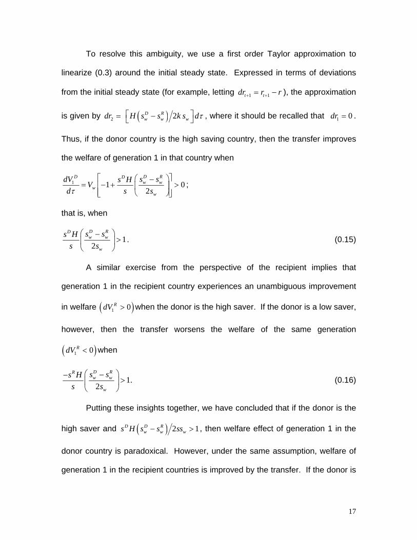
To resolve this ambiguity, we use a first order Taylor approximation to
linearize (0.3) around the initial steady state. Expressed in terms of deviations
from the initial steady state (for example, letting 1 1t tdr r r+ += − ), the approximation
is given by 2dr = ( ) 2D Rw w wH s s k s dτ⎡ −⎣
⎤⎦ , where it should be recalled that 1 0dr = .
Thus, if the donor country is the high saving country, then the transfer improves
the welfare of generation 1 in that country when
1 1 02
D RD Dw w
ww
s sdV s HVd s sτ
⎡ ⎤⎛ ⎞−= − + >⎢ ⎥⎜ ⎟
⎢ ⎥⎝ ⎠⎣ ⎦;
that is, when
12
D RDw w
w
s ss Hs s
⎛ ⎞−>⎜ ⎟
⎝ ⎠. (0.15)
A similar exercise from the perspective of the recipient implies that
generation 1 in the recipient country experiences an unambiguous improvement
in welfare when the donor is the high saver. If the donor is a low saver,
however, then the transfer worsens the welfare of the same generation
when
( 1 0RdV > )
( )1 0RdV <
1.2
D RRw w
w
s ss Hs s
⎛ ⎞−−>⎜ ⎟
⎝ ⎠ (0.16)
Putting these insights together, we have concluded that if the donor is the
high saver and ( ) 2D D Rw w ws H s s ss− 1> , then welfare effect of generation 1 in the
donor country is paradoxical. However, under the same assumption, welfare of
generation 1 in the recipient countries is improved by the transfer. If the donor is
17
the low saver and ( ) 2R D Rw w ws H s s ss− − 1> , then welfare of generation 1 in the
recipient country is worsened by the transfer. Under the same assumption, the
welfare of generation 1 in the donor country is also worsened. The conclusion to
be drawn is that the effects of the transfer on welfare may be viewed as
paradoxical from the perspective of generation 1 in at most one of the two
countries.
Proposition 2: Suppose the initial steady state is at the golden rule. Then,
if the donor is a high saver and ( )2 D D Rw w wH ss s s s> − , then the welfare of
generation 1 in the donor and recipient countries is improved by the transfer. If
the donor is a low saver and ( )2 R D Rw w wH ss s s s> − − , then the welfare of
generation 1 in both the donor and recipient countries is worsened by the
transfer.
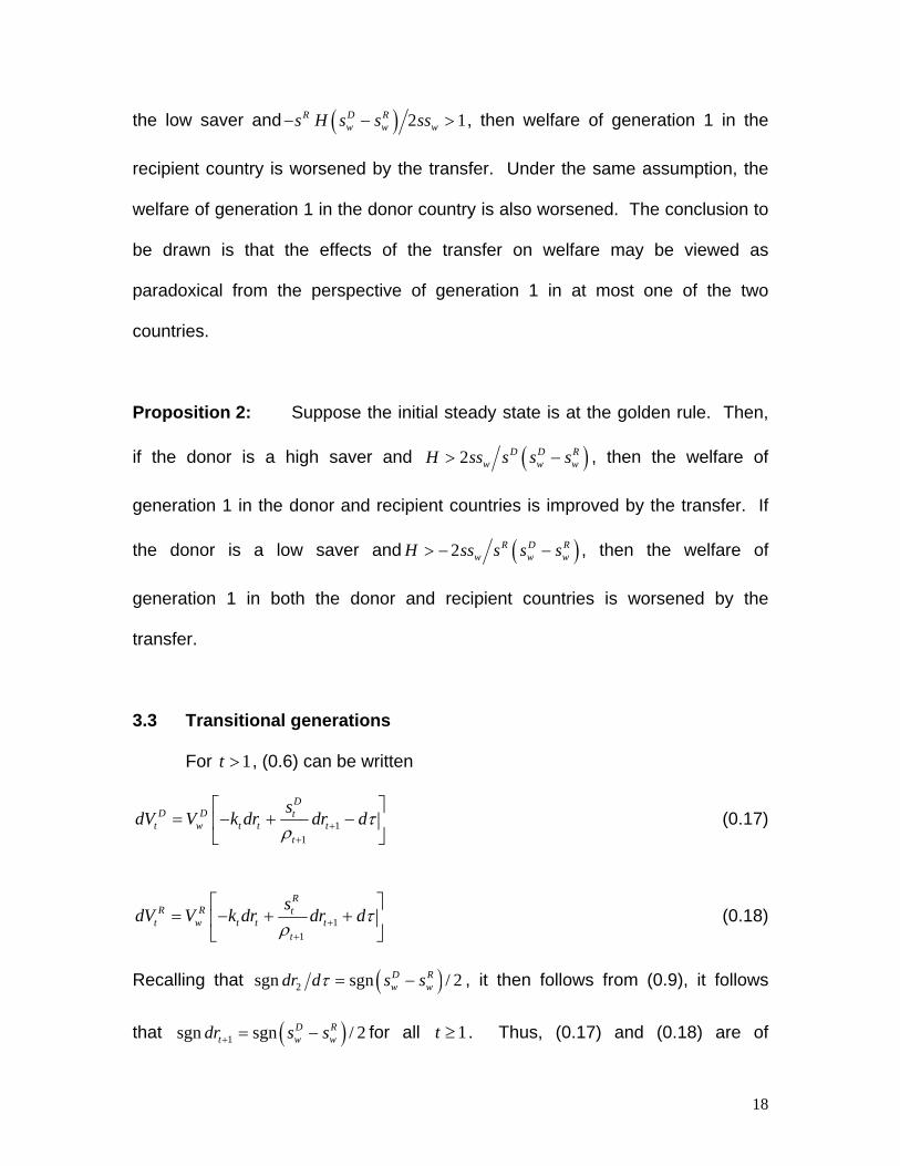
3.3 Transitional generations For 1t > , (0.6) can be written
11
DD D t
t w t t tt
sdV V k dr dr dτ
ρ ++
⎡ ⎤= − + −⎢ ⎥
⎣ ⎦ (0.17)
11
RR R t
t w t t tt
sdV V k dr dr dτ
ρ ++
⎡ ⎤= − + +⎢ ⎥
⎣ ⎦ (0.18)
Recalling that ( )2sgn sgn / 2D R
w wdr d s sτ = − , it then follows from (0.9), it follows
that for all . Thus, (0.17) and (0.18) are of ( )1sgn sgn / 2D Rt w wdr s s+ = − 1t ≥
18
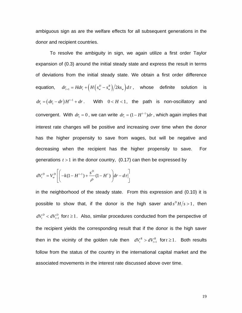
ambiguous sign as are the welfare effects for all subsequent generations in the
donor and recipient countries.
To resolve the ambiguity in sign, we again utilize a first order Taylor
expansion of (0.3) around the initial steady state and express the result in terms
of deviations from the initial steady state. We obtain a first order difference
equation, ( )(1 2D Rt t w w wdr Hdr H s s ks d) τ+ = + − , whose definite solution is
. With 0( ) 11
ttdr dr dr H dr−= − + 1H< < , the path is non-oscillatory and
convergent. With , we can write , which again implies that
interest rate changes will be positive and increasing over time when the donor
has the higher propensity to save from wages, but will be negative and
decreasing when the recipient has the higher propensity to save. For
generations in the donor country, (0.17) can then be expressed by
1 0dr = 1(1 )ttdr H dr−= −
1t >
1(1 ) (1 )D
D D t tt w
sdV V k H H dr dτρ
−⎡ ⎤⎛ ⎞= − − + − −⎢ ⎥⎜ ⎟
⎝ ⎠⎣ ⎦
in the neighborhood of the steady state. From this expression and (0.10) it is
possible to show that, if the donor is the high saver and 1Ds H s > , then
1D D
t tdV dV +< for . Also, similar procedures conducted from the perspective of
the recipient yields the corresponding result that if the donor is the high saver
then in the vicinity of the golden rule then
1t ≥
1R R
t tdV dV +> for . Both results
follow from the status of the country in the international capital market and the
associated movements in the interest rate discussed above over time.
1t ≥
19

To sum this discussion, as well as a similarly constructed argument that
instead assumes that the donor is the low-saving county, we have the following
proposition.
Proposition 3 Suppose the initial steady state is at the golden rule. Then, if the
donor is the high saver and DH s s> or, if the donor is the low saver
and RH s s> , then the effect of a permanent transfer on the welfare of the donor
country is increasing over time, whereas it is decreasing over time for the
recipient country.
4. Discussion
In this section, we summarize the effects of the transfer on the various
generations in both countries and discuss implications regarding the occurrence
of a transfer paradox.
We begin by noting that the sufficient conditions identified by Proposition 2
are stronger than the conditions identified by Propositions 1 and 3.
Corollary If the donor is the high saver and ( )2 D D Rw w wH ss s s s> − , then
DH s s> and 1
2 2
D RD Rw w
w ws ss sH ss ss
−⎡ ⎤⎛ ⎞⎛ ⎞ −−
> +⎢ ⎜ ⎟⎜ ⎟⎢ ⎥⎝ ⎠⎝ ⎠⎣ ⎦
⎥ . If the donor is the low saver
20
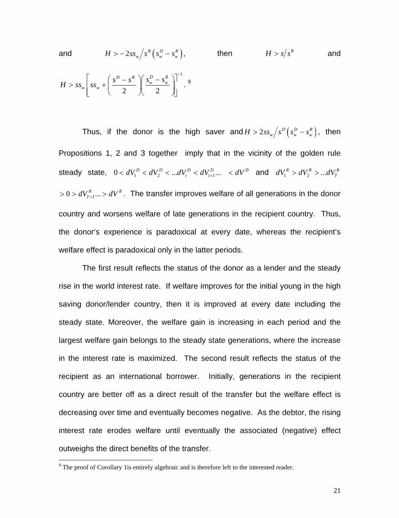
and ( )2 R D Rw w wH ss s s s> − − , then RH s s> and
1
2 2
D RD Rw w
w ws ss sH ss ss
−⎡ ⎤⎛ ⎞⎛ ⎞ −−
> +⎢ ⎥⎜ ⎟⎜ ⎟⎢ ⎥⎝ ⎠⎝ ⎠⎣ ⎦
. 9
Thus, if the donor is the high saver and ( )2 D D Rw w wH ss s s s> −
1
, then
Propositions 1, 2 and 3 together imply that in the vicinity of the golden rule
steady state, 1 20 ... ...D D D Dt tdV dV dV dV +< < < < DdV< and
. The transfer improves welfare of all generations in the donor
country and worsens welfare of late generations in the recipient country. Thus,
the donor’s experience is paradoxical at every date, whereas the recipient’s
welfare effect is paradoxical only in the latter periods.
1 2 ...R RTdV dV dV> > R
R
10 ...RTdV dV+> > >
The first result reflects the status of the donor as a lender and the steady
rise in the world interest rate. If welfare improves for the initial young in the high
saving donor/lender country, then it is improved at every date including the
steady state. Moreover, the welfare gain is increasing in each period and the
largest welfare gain belongs to the steady state generations, where the increase
in the interest rate is maximized. The second result reflects the status of the
recipient as an international borrower. Initially, generations in the recipient
country are better off as a direct result of the transfer but the welfare effect is
decreasing over time and eventually becomes negative. As the debtor, the rising
interest rate erodes welfare until eventually the associated (negative) effect
outweighs the direct benefits of the transfer.
9 The proof of Corollary 1is entirely algebraic and is therefore left to the interested reader.
21

If, instead, the donor is a low saver and ( )2 R D Rw w wH ss s s s> − − , then it
can be shown that in the vicinity of the golden rule,
1 1... 0 ...D D DT TdV dV dV dV+< < < < < D R and .
The transfer worsens the welfare of all generations in the recipient country and
improves welfare for the latter generations in the donor country. Thus, the
recipient’s experience is paradoxical at every date, whereas the donor’s welfare
is affected paradoxically only for the latter periods.
1 20 R RdV dV> > 1... ...R RT TdV dV dV+> > >
The interpretation is, of course, analogous to the previous case. Here, the
donor is a borrower facing an interest rate that is decreasing over time, with a
benefit that eventually exceeds the direct cost of the transfer payment. Also, the
welfare loss experienced by the recipient in the first period is exacerbated at
each subsequent date due to the fact that it is a lender facing a declining rate of
interest.
We now summarize the findings of this section with the following
proposition.
Proposition 4: Suppose the initial steady state is at the golden rule. If the
donor is the high saver and ( )2 D D Rw w wH ss s s s> −
)
, then the welfare of all
generations in the donor country and the early generations in the recipient
country is improved by a permanent transfer, whereas the welfare of the late
generations in the recipient country is worsened. If the donor is the low saver
and (2 R D Rw w wH ss s s s> − − , then the welfare of all generations in the recipient
22
country and the early generations in the donor country is worsened by a
permanent transfer, whereas the welfare of the late generations in the donor
country is improved.
It might be useful, in interpreting Proposition 4, to introduce the notion of a
weak and strong version of the transfer paradox. Suppose a weak transfer
paradox is said to occur at a point in time when either generation in the donor or
the recipient country experiences a paradoxical welfare effect. And, a strong
transfer paradox is said to occur at a point in time when the welfare effects of
both the donor and the recipient countries are paradoxical. Then, Proposition 4
implies that, regardless of assumption regarding the ranking of savings
propensities for the two countries, there are conditions under which the early
periods are characterized by the weak transfer paradox and the late periods by a
strong transfer paradox. The overriding conclusion is therefore that there are
sufficient conditions under which some version of the transfer paradox applies at
every date in the transition to a steady state.
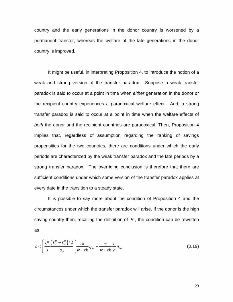
It is possible to say more about the condition of Proposition 4 and the
circumstances under which the transfer paradox will arise. If the donor is the high
saving country then, recalling the definition of H , the condition can be rewritten
as
( ) / 2D RDw w
sww
s ss rk ws s w rk w rk s
rρε η
ρ
⎛ ⎞−⎜ ⎟<⎜ ⎟ + +⎝ ⎠
η− (0.19)
23
where /sw wws sη ≡ and /s s sρ ρη ρ≡ . Thus, the elasticity of substitution cannot
be too large for the transfer paradox to arise. However, the condition for local
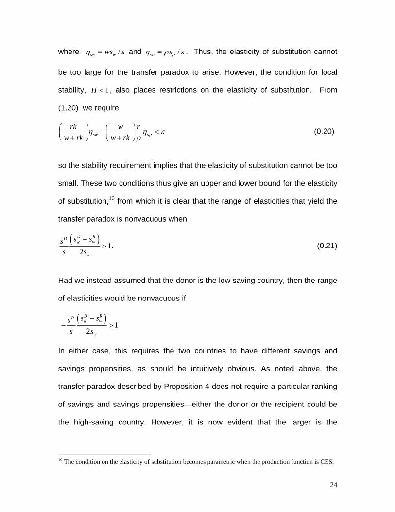
stability, 1H < , also places restrictions on the elasticity of substitution. From
(1.20) we require
sw srk w r
w rk w rk ρη ηρ
⎛ ⎞ ⎛ ⎞−⎜ ⎟ ⎜ ⎟+ +⎝ ⎠ ⎝ ⎠ε< (0.20)
so the stability requirement implies that the elasticity of substitution cannot be too
small. These two conditions thus give an upper and lower bound for the elasticity
of substitution,10 from which it is clear that the range of elasticities that yield the
transfer paradox is nonvacuous when
( )1.
2
D RDw w
w
s sss s
−> (0.21)
Had we instead assumed that the donor is the low saving country, then the range
of elasticities would be nonvacuous if
( )
12
D RRw w
w
s sss s
−− >
In either case, this requires the two countries to have different savings and
savings propensities, as should be intuitively obvious. As noted above, the
transfer paradox described by Proposition 4 does not require a particular ranking
of savings and savings propensities—either the donor or the recipient could be
the high-saving country. However, it is now evident that the larger is the
10 The condition on the elasticity of substitution becomes parametric when the production function is CES.
24
difference in savings and/or savings propensities, the wider is the range of
elasticities that are compatible with the transfer paradox.
Proposition 5: Suppose the initial steady state is at the golden rule. For
intermediate values of the elasticity of substitution, the transition path arising
from a permanent transfer may be characterized by a weak transfer paradox in
the early periods and a strong transfer paradox in the late periods and steady
state, regardless of the ranking of savings rates across countries.
5. Transfers and dynamic efficiency Having demonstrated that the transfer paradox may arise at the golden
rule, we now explore the effects of initial steady states away from the golden rule.
For expedience, we confine our discussion to the welfare effects implied for the
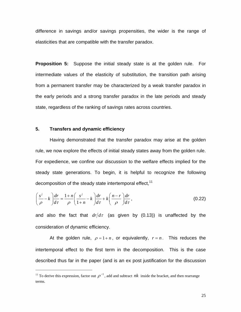
steady state generations. To begin, it is helpful to recognize the following
decomposition of the steady state intertemporal effect,11
11
j js dr n s dr n rk k kd n d
drdρ τ ρ τ ρ
⎛ ⎞ ⎛ ⎞ ⎛ ⎞+ −− = − +⎜ ⎟ ⎜ ⎟ ⎜ ⎟+ ⎝ ⎠⎝ ⎠ ⎝ ⎠ τ
, (0.22)
and also the fact that dr dτ (as given by (0.13)) is unaffected by the
consideration of dynamic efficiency.
At the golden rule, 1 nρ = + , or equivalently, r n= . This reduces the
intertemporal effect to the first term in the decomposition. This is the case
described thus far in the paper (and is an ex post justification for the discussion
11 To derive this expression, factor out 1ρ− , add and subtract inside the bracket, and then rearrange terms.
nk
25
in Section 3.1). Assuming that the conditions for the golden rule transfer paradox
are met, we explore the implications of introducing 1 nρ ≠ + .
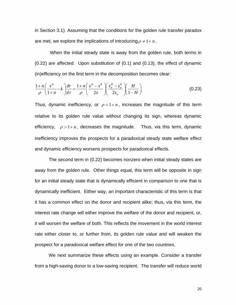
When the initial steady state is away from the golden rule, both terms in
(0.22) are affected. Upon substitution of (0.1) and (0.13), the effect of dynamic
(in)efficiency on the first term in the decomposition becomes clear:
1 11 2 2
D RD D Rw w
w
s sn s dr n s s Hkn d s s Hρ τ ρ
⎛ ⎞⎛ ⎞ ⎛ ⎞ −+ + − ⎛− = ⎜ ⎟⎜ ⎟ ⎜ ⎟ ⎜+ −⎝ ⎠⎝ ⎠ ⎝ ⎠⎝ ⎠ 1⎞⎟ (0.23)
Thus, dynamic inefficiency, or 1 nρ < + , increases the magnitude of this term
relative to its golden rule value without changing its sign, whereas dynamic
efficiency, 1 nρ > + , decreases the magnitude. Thus, via this term, dynamic
inefficiency improves the prospects for a paradoxical steady state welfare effect
and dynamic efficiency worsens prospects for paradoxical effects.
The second term in (0.22) becomes nonzero when initial steady states are
away from the golden rule. Other things equal, this term will be opposite in sign
for an initial steady state that is dynamically efficient in comparison to one that is
dynamically inefficient. Either way, an important characteristic of this term is that
it has a common effect on the donor and recipient alike; thus, via this term, the
interest rate change will either improve the welfare of the donor and recipient, or,
it will worsen the welfare of both. This reflects the movement in the world interest
rate either closer to, or further from, its golden rule value and will weaken the
prospect for a paradoxical welfare effect for one of the two countries.
We next summarize these effects using an example. Consider a transfer
from a high-saving donor to a low-saving recipient. The transfer will reduce world
26
steady state capital accumulation and increase the interest rate. If the initial
steady state is above that of the golden rule, then and the steady state is
dynamically inefficient. As noted, the effect described by the first term in (0.22) is
intensified and thus independently increases the possibility of a strong transfer
paradox. The second term introduces an additional positive effect on welfare in
both countries. For the donor, both terms reflect an increase welfare above and
beyond that discussed in the golden rule case, thus ensuring a paradoxical
welfare effect. For the recipient, the two terms instead imply conflicting effects,
and the overall welfare change is now ambiguous. Thus, with the introduction of
dynamic inefficiency, the possibility of a strong transfer paradox remains.
Moreover, in cases where the strong paradox does not obtain, there will instead
be a weak transfer paradox characterized by a welfare-improvement in both
countries.
n r>
If the initial steady state is instead dynamically efficient—that is, if n r< ,
the same transfer would weaken the intensity of the first term without changing
its sign, and, introduce an additional negative welfare effect common to both
countries. Overall, the welfare effects are now ambiguous for the donor and
unambiguously negative for the recipient. Thus, the implications for the transfer
paradox are symmetric to those above. The strong transfer paradox cannot be
ruled out by dynamic efficiency, and, when it does not obtain, a weak transfer
paradox characterized by mutual welfare deterioration will arise.
To sum, even when initial steady states are away from the golden rule, the
possibility of the strong transfer paradox cannot be ruled out on theoretical
27
grounds. However, the additional effect introduced by the movement of the world
capital-labor ratio either towards or away from the golden rule, generates either a
mutual welfare improvement or deterioration for the two countries, either of which
tend to decrease prospects for the strong paradox and lend support to the weak
version of the transfer paradox.12
6. A parametric example
We now demonstrate our results concerning the transfer paradox using a
parameterized version of the model. However, as there is no convincing
evidence that actual economies operate at or beyond the golden rule (see Abel
et al (1989)), we will confine our attention to a case involving an initial steady
state that is dynamically efficient. As noted above, relative to an initial steady
state at the golden rule capital-labor ratio, this assumption tends to work against
the strong version of the transfer paradox, and in favor of the weak transfer
paradox. Also, this assumption implies that the steady state welfare effects
cannot be identified via the sufficient conditions identified by the propositions, but
rather must be derived from the more general welfare expressions, (0.7) and
(0.8). Our example highlights that, under different specifications of the saving
rate, both strong and weak versions of the transfer paradox may arise.
12 These arguments can be made explicit. The transfer under consideration improves the donor’s welfare (and worsens the recipient’s welfare) in a steady state away from the golden rule when (0.22) exceeds 1.
Now, (0.13) implies that ( ) ( ) ( ) ( ) ( )/ / 2D Rw w wk n r dr d n r s s s H Hρ τ ρ ⎡ ⎤⎡ ⎤ ⎡ ⎤− = − −⎣ ⎦ ⎣ ⎦ ⎣ ⎦ 1− .
Together with(0.23), the inequality becomes ( ) ( )1 2 (1 ) 1D R Dw w wH s s s n s sρ 1⎡ ⎤⎡ ⎤+ − + −⎣ ⎦ >⎣ ⎦ .
Clearly, 1 nρ > + works against the transfer paradox but is not by itself enough to negate the inequality. Similarly, it can be shown that 1 nρ < + is not sufficient to negate the possibility of the recipient being worse off.
28
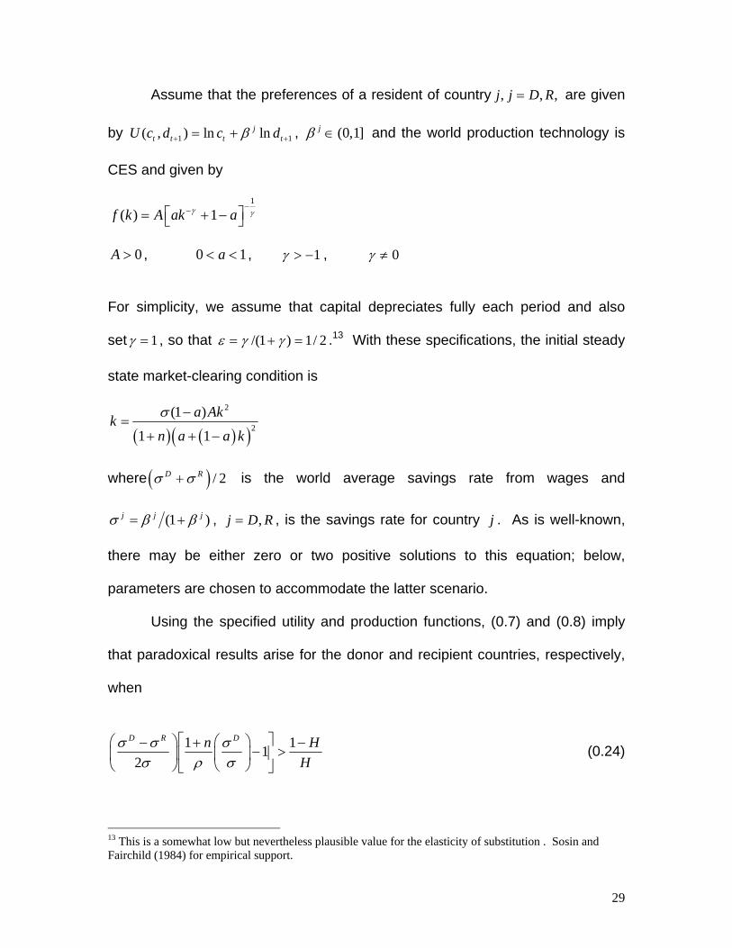
Assume that the preferences of a resident of country are given
by , and the world production technology is
CES and given by
, ,j j D R= ,
( , ) ln lnjt t t tU c d c dβ+ = + (0,1]jβ ∈1 1+
1
( ) 1f k A ak aγ γ−−⎡ ⎤= + −⎣ ⎦
0A > , , 0 1a< < 1γ > − , 0γ ≠
For simplicity, we assume that capital depreciates fully each period and also
set 1γ = , so that /(1 ) 1/ 2ε γ γ= + = .13 With these specifications, the initial steady
state market-clearing condition is
( ) ( )( )2
2
(1 )
1 1
a Akkn a a k
σ −=
+ + −
where is the world average savings rate from wages and ( / 2D Rσ σ+ )
(1 )j j jσ β β= + , , is the savings rate for country ,j D R= j . As is well-known,
there may be either zero or two positive solutions to this equation; below,
parameters are chosen to accommodate the latter scenario.
Using the specified utility and production functions, (0.7) and (0.8) imply
that paradoxical results arise for the donor and recipient countries, respectively,
when
1 1
2
D R Dn HH
σ σ σσ ρ σ
⎡ ⎤⎛ ⎞ ⎛ ⎞− + −− >⎢ ⎥⎜ ⎟ ⎜ ⎟
⎝ ⎠ ⎝ ⎠⎣ ⎦
1
(0.24)
13 This is a somewhat low but nevertheless plausible value for the elasticity of substitution . Sosin and Fairchild (1984) for empirical support.
29

112
D R RnH
σ σ σσ ρ σ
⎡ ⎤⎛ ⎞ ⎛ ⎞− +− >⎢ ⎥⎜ ⎟ ⎜ ⎟
⎝ ⎠ ⎝ ⎠⎣ ⎦
1 H−
k a
(0.25)
where and ( )1 / (1 ) /n aρ σ+ = − ( )( )(1 ) / 1 / 2H H a k a− = − − a . To calibrate the model, we set 0.7a = and 0.36σ = (equivalently,
0.5625β = ), which respectively imply a capital’s share of 0.29 at the initial steady
state, and a quarterly average discount factor of 0.99 for a generation of 30 years
duration. Also, we set the scale parameter to 20A = and the population growth
rate to ; the former admits two positive steady states and the second
implies an annual growth rate for total output of 2.5%. Under these parameter
values the unique stable steady state is
1.097n =
5.8471k = , where 0.57 1H = < . At this
initial steady state, world savings as a fraction of production is 26%, and the
generational interest rate is 1.3245 (which is equivalent to an annual rate of
approximately 2.85%). The latter is therefore consistent with a dynamically
efficient initial steady state.
We further assume that the donor country is the high saving country and,
noting that the transfer paradox is more likely to arise under large differences in
the country-specific savings rates, set and .0.71Dσ = 0.01Rσ = 14 With these
specifications, the left hand side of (0.24) and (0.25) equal 0.7576 and 0.9479,
respectively. The common right hand side of these expressions equals 0.7530.
Thus, both inequalities are satisfied and this parameterization is consistent with a
14 This implicitly assumes corresponding differences in the jβ s. Also, when expressed as a fraction of domestic and national product, the domestic savings rate of the donor falls to a more reasonable .5 and .4 respectively.
30
strong transfer paradox, despite the fact that the initial steady state is
dynamically efficient.
Admittedly, the assumed values for the world savings rate and the savings
rate of the donor country, are somewhat high.15 If, other things equal, we instead
set 0.3σ = , and ,0.59Dσ = 0.01Rσ = 16 then there is again a positive stable initial
steady state, (with 3.133k = 0.86H = <1) but the left hand sides of (0.24) and
(0.25) now equal -0.2009 and 0.9537 respectively, whereas the right hand side
equals 0.1714. Thus, with this change, only the recipient will experience a
paradoxical welfare effect. In this case, the weak transfer paradox arises and
welfare is reduced in both countries.
7. Conclusion
In this paper we have analyzed the effects of an international income
transfer on world capital accumulation and the welfare for both the donor and the
recipient countries. We find that, if the initial steady state occurs at the golden
rule capital-labor ratio, then a strong transfer paradox is possible at, and in a
neighborhood of, the steady state. Moreover, a weak transfer paradox may
characterize all earlier dates. The strong paradox cannot be ruled out by an
initial steady state that is instead away from the golden rule, although there is
increased likelihood that the weak version of the transfer paradox will
characterize the steady state.
15 These savings rates are high, but not unheard of. Several East Asian economies, including China and Singapore, have had national savings rates in excess of 40%. 16 In this case, the world savings rate when expressed as a fraction of production is 17%, and national savings when expressed as a fraction of national income are 23% and just under 1% for the donor and recipient respectively.
31

We close with a few remarks related to transfers as we have described
them in Section 4. The potential discrepancy between the long and short-run
effects of transfers, namely, the difference between the strong and weak transfer
paradox, has particular interest when considered in a political context. Thus far
we have regarded the transfer as a policy that has been committed to, by the
donor and recipient alike, in the first period of time. As has been shown, the
donor may in fact benefit from this policy at all dates following its adoption,
whereas the recipient may benefit from the policy only in the short-run. Whereas
the donor’s commitment to the policy is then consistent with welfare
maximization, the recipient’s participation is instead subject to time
inconsistency: on welfare grounds, the recipient has incentive to adopt the policy
in the initial period and then renege on it at a later point in time. Moreover, if the
donor believes the recipient suffers from myopia, then these welfare results could
also justify a skeptical perspective towards the actual benevolence of donors
whose benefits outlast those of their recipients.
32

References
Abel, A, N. Mankiw, L. Summers and R. Zeckhauser (1989) `Assessing Dynamic Efficiency: Theory and Evidence.” Review of Economic Studies 56 (January): 1-20. Bhagwati, J and R. Brecher (1982) `Immiserizing transfers from abroad’ Journal of International Economics 13: 353-364. Bhagwati, J., R. Brecher and T. Hatta (1983) `The generalized theory of transfers and welfare: bilateral transfers in a multilateral world’ American Economic Review 73(4): 606- 618. Bhagwati, J., R. Brecher and T. Hatta (1985) `The generalized theory of transfers and welfare: exogenous (policy-imposed) and endogenous (transfer-induced) distortions,’ The Quarterly Journal of Economics 100(3): 697-714. Diamond, P. (1965) `National Debt in a Neoclassical Growth Model,’ American Economic Review 55(5):1126-1150. Gale, D. (1974) `Exchange equilibrium and coalitions: an example,’ Journal of Mathematical Economics, 1:63-66. Galor, O. and H.M. Polemarchakis (1987) `Intertemporal equilibrium and the transfer paradox,’ Review of Economic Studies LIV: 47-156. Galor, O. and Harl E. Ryder (1989) `Existence, uniqueness, and stability of equilibrium in an overlapping-generations model with productive capital,’ Journal of Economic Theory 49:360-375.
Haaparanta, P. (1989) `The intertemporal effects of international transfers,’ Journal of International Economics 26:371-382. Sosin, K. and L. Fairchild (1984) `Nonhomotheticity and technological bias in production.’ Review of Economics and Statistics 66(1): 44-50. Tan, K-H. (1998) `International transfers from rich to poor nations,’ Review of International Economics 6(3):461-471. Yanagihara, M. (2006) `The strong transfer paradox in an overlapping generations framework,’ Economics Bulletin 1(3):1-8. Yano, M. (1983) `Welfare aspects of the transfer problem,’ Journal of International Economics 15: 277-289.
33