5757 S. University Ave., Chicago, IL 60637 | Main: 773.702.5599 | bfi.uchicago.edu

Ronzetti Initiativefor the Study ofLabor Markets

WORKING PAPER · NO. 2019-121

A Cross-Cohort Analysis of Human Capital Specialization and the College Gender Wage GapCarolyn Sloane, Erik Hurst, and Dan BlackOCTOBER 2019

A Cross-Cohort Analysis of Human Capital

Specialization and the College Gender Wage Gap ∗

Carolyn Sloane Erik Hurst Dan Black

September 29, 2019

Abstract

This paper explores the importance of pre-market human capital specialization in ex-plaining gender differences in labor market outcomes among the highly skilled. Usingnew data with detailed undergraduate major information for several cohorts of Amer-ican college graduates, we establish many novel facts. First, we show evidence of agender convergence in college major choice over the last 40 years. Second, we highlightthat women today still choose college majors associated with lower potential wages thanmen. Third, we report gender differences in the mapping from major to occupation.Even conditional on major, women systematically choose lower potential wage andlower potential hours-worked occupations than men. Fourth, we document a modestgender convergence between the 1950 and 1990 birth cohorts in the mapping of majorto occupation. Finally, we show that college major choice has strong predictive powerin explaining gender wage gaps independent of occupation choice. Collectively, ourresults suggest the importance of further understanding gender differences in pre-labormarket specialization including college major choice.

∗We thank seminar participants at the University of Chicago for helpful comments. Author affiliationand contact information: Carolyn Sloane, University of California, Riverside, csloane@ucr.edu; Erik Hurst,University of Chicago Booth School of Business, erik.hurst@chicagobooth.edu; and Dan Black, University ofChicago, Harris School of Public Policy, danblack@uchicago.edu.

1 Introduction

There is an extensive literature studying the fundamental changes to women’s labor market

outcomes in the U.S. during the post-War period.1 Some of this literature has documented

the phenomenal growth in the relative supply of college-educated women.2 This shift has

changed the gender composition of the college-educated labor force. At the same time,

the specialized skills of college-educated men and women have also been evolving. While

post-schooling labor market specialization (e.g. occupational choice) has been identified as

an important determinant of gender gaps in wages and employment, the impact of pre-

market specialization (e.g. major choice) has not received as much attention.3 The menu

of major choices offered by US post-secondary institutions is large. Given changes over

time in occupational specialization, we suspect that cross-cohort dynamics in pre-market

specialization may be important. Until recently, large, multi-cohort data linking detailed

college major choice to subsequent labor market outcomes was not previously available. Due

to this empirical constraint, there is relatively little work on the impact of pre-market human

capital specialization on gender wage gaps among the highly-educated across cohorts.

In this paper, we use new data to explore the importance of gender differences in pre-

labor market specialization on gender differences in labor market outcomes. Specifically, the

paper addresses the following four questions: (1) To what extent have the pre-labor market

human capital specialization decisions of college-educated men and women converged over

time? (2) Does gender influence the mapping of college major to subsequent occupational

specialization and has this mapping changed over time? (3) How much of college gender

wage and employment gaps can be attributed to major choice independent of occupational

choice? (4) How has the relationship between major choice and gender wage and employment

gaps evolved over time?

To address the above questions, we exploit newly released data from the American Com-

munity Survey (ACS) which added questions starting in 2009 on pre-labor market special-

ization, namely major choice, for millions of college-educated individuals.4 These questions

1See, for example, Altonji and Blank (1999), Bertrand and Hallock (2001), Black and Juhn (2000), Blauand Kahn (1997), Blau and Kahn (2000), Goldin (1992), and Jacobsen et al. (1999). For a recent, detailedreview of this literature, see Blau and Kahn (2017).

2See Becker et al. (2010), Charles and Luoh (2003), DiPrete and Buchmann (2006), Goldin et al. (2006),and Jacob (2002).

3The literature documenting both changes in occupational sorting by gender over time and the contri-bution of occupational choice to gender labor market disparities includes Bayard et al. (2003), Blau et al.(1998), Blau et al. (2014), Cortes and Pan (2018), Goldin (1992), Groshen et al. (1987), Hsieh et al. (2019),Macpherson and Hirsch (1995), and Pan (2015).

4The ACS has been used by Altonji et al. (2014) to measure the evolution of wage inequality within majorand Altonji et al. (2016) to estimate major-specific returns.

1

are asked regardless of age. This allows us to explore how pre-labor market human capital

specialization decisions have changed across cohorts.

We begin by assessing the extent to which men and women choose different college ma-

jors and how those differences have evolved over time. We document that women made

substantial progress in traditionally male-dominated majors such as business and the phys-

ical and life sciences. Younger birth cohorts of women are even more likely to be biology

majors than men. In contrast, although relative growth of women in engineering is large,

engineering remains a male-dominated field of study. The fraction of women majoring in

education, a historically female-dominated field of study, declined substantially. However,

the decline among males was even larger making the education field even more heavily

female-concentrated among recent birth cohorts.

In addition to using traditional indices to summarize trends in gender segregation, we

develop a new index that measures the potential wage gap between women and men based

on major choice. We define a major’s potential wage based on the median log hourly wage

of native, white men aged 43-57 who matriculated with that major. With this measure, we

compare the major choice of women relative to the major choice of men for each birth cohort

where the units of the index are in potential log wage differentials. We find that across

all birth cohorts women systematically choose majors with lower potential wages relative

to men. College-educated women born in the 1950s matriculated with majors that had

potential wages that were 12% lower than men from their cohort. That gap fell to about

9% for the 1990 birth cohort. While there has been convergence in major choice between

men and women during the last 40 years, the youngest birth cohorts of women still choose

majors with lower potential wages than men. We also highlight that the trend in the gender

similarity of major choice is non-monotonic with much of the convergence occurring between

the 1950 and 1975 birth cohorts with a modest divergence for recent cohorts.

In the next part of the paper, we measure gender differences in the mapping of college

major to subsequent occupational specialization and explore how this mapping has changed

over time. We show that convergence in major choice is of a similar order of magnitude

as the convergence in occupational choice. While women systematically are in lower wage

occupations conditional on major choice, this gap has narrowed over time. For example,

for the 1950 birth cohort, women who majored in engineering chose subsequent occupations

with potential wages that were 14 percent lower than men from their cohort who majored in

engineering. For the 1990 birth cohort, however, women who majored in engineering ended

up working in occupations with roughly the same potential wages as men who majored in

engineering. These patterns have nothing to do with women earning less than men within

an occupation as we only measure an occupation’s potential wages based on what men earn

2

in that occupation. These patterns stem from the fact that the subsequent occupations

chosen by women who majored in engineering used to differ markedly from men but now the

occupational choice conditional on major has converged.

The patterns for engineering are broadly similar to the patterns for all majors. For

the 1950 birth cohort, women chose occupations conditional on major choice with poten-

tial wages that were about 11% lower than comparable men with the gap being larger for

higher potential wage majors (like biochemical engineering and economics). The gender

gap in occupational choice conditional on major narrowed meaningfully for recent cohorts.

Interestingly, we find this convergence is driven by movements of women at the top of the

major-pay distribution into higher-pay occupations.

These results show that not only has their been a gender convergence in pre-labor market

specialization (college major) and post-schooling specialization (occupational choice), there

has also been a gender convergence in the mapping from major choice to occupation. Com-

pared to their predecessors, younger women are in occupations that are closer in potential

wages to those chosen by male peers with the same major. We also show that the poten-

tial desire for lower hours worked on the part of women explains part, but not all, of these

patterns.

In the final part of the paper, we ask how much of the gender gap in wages can be

explained by controlling for both undergraduate major and for current occupational choice

and how these relationships have evolved over time. We do this for all cohorts pooled together

and separately by 10-year birth cohorts. The latter analysis lends itself to a decomposition

exercise to assess how much of the change in gender wage gaps can be explained by changes

in undergraduate major choice and current occupational choice. We find that the gender

gap in wages for all college-educated cohorts in the 2014-2017 ACS was 23 log points after

controlling for simple demographics such as highest degree completed, age, race, and state of

residence. Further controlling for both major choice and current occupation reduced the wage

gap to only 11 log points - a 50% reduction. Most importantly, we find that controlling for

major choice has strong predictive power above and beyond controlling for just occupational

choice. The gender gap in wages controlling for demographics and occupational choice is

14.3 log points. Adding undergraduate major as a control in addition to occupation and

demographics further reduces the gender wage gap by 3 log points. We then compare recent

(1978 to 1987) birth cohorts to older cohorts (1958 to 1967). We document that the role

of college major in these cohorts remains remarkably stable, but there is a sharp reduction

in the importance of occupation. Over all, we find that controlling jointly for major choice

and occupational choice explains roughly 40 percent of the cross-birth cohort decline in the

wage gap.

3

Finally, we document that undergraduate major choice does not have any effect on exten-

sive margin labor market participation for college graduates. While undergraduate major is

informative about gender wage differentials, it is not informative with respect to explaining

extensive margin differences in labor supply. However, we document heterogeneous effects

by gender on intensive margin participation. Specifically, we find that conditional on college

major choice, women select into occupations with lower annual hours worked than men.

Our results complement a literature on gender differences in major choice. This litera-

ture has followed two separate strands. First, there is a recent literature documenting gender

differences in major choice and how those differences have evolved over time. Dickson (2010)

uses administrative data from three public universities in Texas and Zafar (2013) uses ad-

ministrative data from Northwestern University to document gender differences in majors for

one cohort of undergraduates at their respective universities. Using data from the National

Center of Education Statistics, England and Li (2006) and Blau et al. (2014) (Chapter 8)

document how gender differences in detailed undergraduate majors have diminished over

time for a nationally representative sample of undergraduates with detailed measures of field

of study. Unfortunately, the data that England and Li (2006) and Blau et al. (2014) use has

no information on subsequent labor market outcomes 5

Second, there is a separate literature examining how gender differences in major choice

affect gender differences in earnings. In a classic reference, Brown and Corcoran (1997) use

data from the 1984 Survey of Income and Program Participation (SIPP) and the National

Longitudinal Study of High School Class of 1972 (NLS72) to document how course work

differences between men and women affect gender wages gaps. For the older cohorts (those

born prior to 1960 and, thus, prior to the female overtaking in college completion), they

find that the gender wage gap for college graduates falls once controlling for 20 broad major

categories. Loury (1997) uses data from the NLS72 and the High School and Beyond Senior

Cohort (Class of 1980) to also document that controlling for GPA and four broad major

choice categories reduces the gender wage gap.6

The goal of our paper is to link and expand on these two strands of the literature.

Specifically, we ask how changes in the gender gap in major choice explain changes in col-

5The literature documenting the under-representation of women in STEM fields includes see, for example,Leslie et al. (1998) and the cites within. Ceci et al. (2014) use data from the National Center for Scienceand Engineering Statistics to highlight the gender convergence in STEM majors. Turner and Bowen (1999)uses data from the College and Beyond database to assess gender differences in major choice within twelveacademically selective colleges and universities finding even conditional on SAT scores, gender differences inmajor choice remain.

6Black et al. (2008) use data from the 1993 National Survey of College Graduates to examine the extent towhich pre-labor market factors (including undergraduate major) explains differences in wages across variousrace-gender groups of college graduates. Their data end in 1990, about the time women’s field of studyingstarted diverging from men.

4

lege gender wage gap over the last half century within the United States. We are able to do

this by exploiting new data that links undergraduate major and labor market outcomes for

many birth cohorts. As a result, we are able to document long-run trends for a nationally

representative sample of college graduates. Throughout, we assess the extent to which un-

dergraduate major has predictive power above and beyond occupational choice. In doing so,

we present novel results on gender differences in the mapping between undergraduate major

and occupational choice. Finally, unlike others in the literature, we examine the extent to

which differences in undergraduate major can explain gender differences in extensive and

intensive margin labor market participation of college graduates. We end the paper with a

discussion of the interpretation of our results.

2 Data

Our primary data source is the 2014-2017 American Community Survey (ACS).7 Starting in

2009, the ACS asked all respondents with a bachelor’s degree to report their undergraduate

major. Given the possible impact of the Great Recession on undergraduate majors, we re-

strict our analysis to only include ACS respondents from the 2014-2017 surveys. Specifically,

our base sample includes roughly 1.7 million observations of individuals aged 23 to 67 with

a bachelors’ degree who reported their undergraduate major.8

Respondents are asked to report their undergraduate field of study. For those respondents

with a post-bachelor’s degree, no additional information is provided for the field of study

of their advanced degree(s). If individuals have more than one bachelor’s degree or more

than one major, they are prompted to list multiple majors. The ACS separately records

up to two separate majors for each respondent. Only 11% of our sample reports having a

second major. For the sample years 2014-2017, the ACS combines major responses into 176

distinct “detailed” majors. The ACS also aggregates these detailed majors into 29 “broad”

major categories. Examples of the detailed majors include journalism, economics, chemical

engineering, molecular biology, music, and finance while examples of the corresponding broad

major fields include communications, social sciences, engineering, biology/life sciences, fine

7The ACS is conducted by the U.S. Census Bureau. The ACS samples roughly 1 percent of the U.S.population each year asking detailed questions on demographics, labor market variables and family structure.We downloaded the ACS samples from IPUMS USA database. For additional details, see Ruggles et al.(2019).

8Of those with a bachelor’s degree, 91.5% of ACS respondents between the ages of 23 and 67 reportedat least one undergraduate major. For those with missing majors, the ACS imputes the majors for theseindividuals by assigning them a major probabilistically based on the reports of other respondents of similarsex, race and occupation. The fraction with missing major was relatively constant between the ages of 23and 67 but did increase sharply for respondents over 75. We exclude those with imputed majors. For moredetails, see the Online Appendix.

5

arts, and business. We assign one undergraduate major to each individual with at least a

bachelor’s degree. For those with only one major, it is the major reported. For those with

two majors, we choose the reported major that is associated with the highest median male

labor market wage.9

Our analysis explores the independent contributions of educational and occupational

specialization decisions to the college gender wage gap and explores gender differences in

the mapping between undergraduate majors and occupational choice. For the 2014-2017

data, we use the reported occupation for all individuals in our sample with a valid, civilian

occupation code who have worked within the previous 5 years.10 Lastly, we use the data

on wages and employment rates from the ACS. We define real wages within the ACS by

dividing self reported annual labor income by self reported annual total hours worked and

then using the CPI to convert into real 2018 dollars. We classify individuals in our sample

as strongly attached to the labor market if the individual reports working at least 30 hours

per week for at least 27 weeks in the previous year. See the Online Appendix for additional

details about the construction of all variables used in the paper.

3 The Convergence in Major Choice

In this section, we document the presence and evolution of gender gaps in undergraduate

major choice and how those gaps have evolved over time. For comparison, we also document

trends in relative occupational choice for college-educated men and women.

For each survey year between 2014 and 2017, we begin by assigning each individual a 5-

year birth cohort based on current age in the survey year.11 In the U.S., most individuals who

ever complete a bachelor’s degree do so by their mid-twenties; this implies that undergraduate

major is largely fixed over the life cycle. Figure 1 graphs the ratio of females to males within

a broad major category.

The majors in Figure 1 highlight the heterogeneity with respect to the gender composition

of broad major fields. For some majors, there has been substantial gender convergence across

birth cohorts. For example, for the 1950 birth cohort, the engineering major contained twenty

men for every one woman. Today, the engineering major is still much more male-dominated,

but that gap has narrowed over time. By the 1990 birth cohort, there were five men for every

9In computing potential wage for each major, we restrict the analysis to a sample of native, white menbetween the ages of 43 and 57 with strong attachment to the labor market in the prior year.

10We use a balanced panel of detailed occupation codes based on the 1990 Census detailed occupationcodes following (Dorn, 2009). This yields 251 detailed occupation codes in our analysis.

11We center the 5-year birth cohorts around years that are multiples of five. For example, what we referto as the 1950 birth cohort includes all individuals born between 1948 and 1952.

6

Figure 1: Gender Differences in Selected Majors by Birth Cohort

0.0

0.2

0.4

0.6

0.8

1.0

1.2

1.4

1.6

1950 1955 1960 1965 1970 1975 1980 1985 1990

Fem

ale

Shar

e/M

ale

Shar

e

Five Year Birth Cohort

Biology/Life Sciences Business History Physical Sciences Engineering

1.0

2.0

3.0

4.0

5.0

6.0

7.0

1950 1955 1960 1965 1970 1975 1980 1985 1990

Fem

ale

Shar

e/M

ale

Shar

e

Five Year Birth Cohort

Nursing/Pharmacy Education Psychology Foreign Languages Fine Arts

Panel A: Historically Male Panel B: Historically FemaleDominated Majors Dominated Majors

Notes: These figures plot the ratio of females to males within major category. The left panel shows trendsfor a set of majors where men outnumber women. The right panel shows trends for a set of majors wherewomen outnumber men. Data from the 2014-2017 ACS and is restricted to those with at least a bachelor’sdegree. See text for additional details.

one woman in the engineering major. These patterns are shown in the solid line in Panel

A. Similar convergence patterns are seen for the physical sciences (e.g., chemistry, physics,

astronomy) and for the biology/life sciences majors (e.g., biology, molecular biology, genetics,

ecology). In fact, biology/life sciences switched from being a major field dominated by men

(for the 1950-1970 birth cohorts) to one dominated by women (the 1980-1990 birth cohorts).

The business major displays a different pattern: women converged toward men between

the 1950-1965 birth cohorts and then diverged thereafter. History was male-dominated

historically and experienced little convergence or divergence over subsequent birth cohorts.

Similar heterogeneity in trends are seen in historically female-dominated majors (Panel

B). There was gender convergence over time in the nursing/pharmacy major. In the 1950

birth cohort, there were five women for every one man in this major. For the 1990 birth

cohort, there less than four women for every one man in this major.12 Notable gender

convergence was also seen in both the foreign language and fine arts majors. Like history,

the education major saw little convergence or divergence between women and men over the

last 50 years. Psychology majors, however, were more likely to be populated by women in

the 1950 cohort and became even more female-intensive by the 1990 cohort.

12The broad major field referred to as “Nursing/Pharmacy” represents a broad category of health-relatedmajors: nursing, pharmacy, treatment therapy professions, community and public health, and miscellaneoushealth medical professions.

7

As seen in Figure 1, some majors moved closer to gender parity and others moved further

from parity from the 1950 to 1990 birth cohorts. We perform two exercises to summarize the

trend in overall similarity in major choice by gender across cohorts. Define smg,c as the share

of gender group g born in 5-year birth cohort c who matriculated with undergraduate major

m. First, we compute a re-normalized Duncan-Duncan segregation index of undergraduate

major segregation by gender and cohort (Duncan and Duncan (1955)). Specifically, we

compute:

IMc = 1− 1

2

M∑m=1

∣∣smmale,c − smfemale,c

∣∣ (1)

where IMc is the re-normalized gender segregation index in major choice for cohort c and

where M is the total number of detailed undergraduate majors reported in the ACS. We

re-normalize the segregation index such that perfect major segregation by gender yields an

index of 0 and perfect major integration by gender yields a Duncan-Duncan index of 1. The

re-normalization implies that an increase in IMc indicates increasing convergence in major

choice by gender. We similarly define IOc , the re-normalized occupational segregation index

based on observed gender differences in occupational sorting.

Segregation indices have some notable shortcomings. The first is that these indices are

invariant to rank (such as an earnings ordering) of the major field or occupation. In other

words, the above segregation index tells us to what extent college-educated men and women

have sorted into similar majors (occupations), but would take on the same value if all men

were chemical engineering majors and all women were fine arts majors as it would if all

men were chemical engineering majors and all women were biomedical engineering majors.

Second, the units of the segregation index do not lend themselves easily to an economic

interpretation. As an alternative measure, we develop an index of the impact of gender on

potential wages based on pre-market educational specialization. In contrast to the segre-

gation index, the units of this index are in wage space allowing for the influence of major

rank and thus making it easier to interpret the economic magnitude of gender differences

in major choice. Furthermore, the inputs of this index are useful in the ensuing empirical

analysis of the college gender wage gap. A crucial input is Y mmale, a potential wage based on

major that is plausibly unaffected by post-educational factors. Specifically, we define Y mmale

to be the median within-major labor market log wage of a group we assume faces minimal

post-educational frictions in the labor market: native, white men between the ages of 43 and

57 with strong attachment to the labor market.13 For example, for anyone (male or female)

13Market effects, such as discrimination, can affect equilibrium wages of groups that do not directly facediscrimination such as white men. In fact, Hsieh et al. (2019) documents that discrimination against women

8

who majored in economics, we assign as their potential wage the median log wage of older

native white men who majored in economics. We formally define the potential wage index

as:

IP,Mc =

∑Mm=1 s

mfemale,cY

mmale∑M

m=1 smmale,cY

mmale

− 1 (2)

where IP,Mc measures the differential “potential” log wage of women of cohort c given

that the female distribution of major choice in a given cohort may differ from males in their

cohort. A value of IP,Mc = 0 means that the major choices of women yield the same potential

log wage as their male counterparts. A value of IP,Mc < 0 implies that women systematically

choose majors associated with lower relative potential log wages. For example, IP,Mc = −0.35

implies that women choose majors that reduce their potential wage by 35 percent relative to

males from a similar cohort. As with our re-normalized Duncan-Duncan index, an increase

in IP,Mc implies that major choice is converging between men and women.

The solid line in Panel A of Figure 2 shows the trend in IMc , measuring major similarity

across different birth cohorts. For the 1950 birth cohort, IMc = 0.55. The index increased to

0.64 for the 1990 birth cohort. Over the last half century, the US saw sharp convergence in

undergraduate major choice by gender measured by the segregation index. The time series

trend in the segregation index however is non-monotonic with the increased convergence

occurring between the 1950 and 1965 birth cohorts. Notably, there is a reversal in the index

for recent cohorts, and this reversal seems to be increasing among more recent cohorts. As

seen in Figure 1, business and psychology majors saw gender divergence for recent cohorts.

Nevertheless, the recent divergence is small relative to the convergence that occurred for older

cohorts implying that major choice overall converged between men and women between the

1950 and 1990 cohorts. During this time period, the fraction of women with a bachelor’s

degree has increased relative to men.14

The solid line in the Panel B of Figure 2 shows the trend in IP,Mc across cohorts. Like

the re-normalized segregation index, the “potential wage” index also shows a strong gender

convergence in major choice over the last half century. This index allows us to interpret

the economic magnitudes of the gender convergence in college major choice over the last

half century. For the 1950 birth cohort, women chose majors that reduced their potential

and blacks in the labor market raises the wages of white men. However, Hsieh et al. (2019) also estimatethat these wage effects on men are small.

14We have performed a series of robustness exercises on the patterns in Figure 2. The hump-shapedpattern in IMc across cohorts persists for different levels broad and detailed majors and when we restrict thesample to include only those with strong attachment to the labor market. For more detail, see the OnlineAppendix.

9

Figure 2: Gender Similarity in Major Choice and Occupation by Cohort

0.44

0.48

0.52

0.56

0.60

0.64

0.68

0.72

0.76

1950 1955 1960 1965 1970 1975 1980 1985 1990

Inve

rse

Dun

can-

Dun

can

Sim

ilari

ty In

dex

Five Year Birth Cohort

Major Occupation

-0.15

-0.14

-0.13

-0.12

-0.11

-0.10

-0.09

-0.08

-0.07

1950 1955 1960 1965 1970 1975 1980 1985 1990

Pote

ntia

l Inc

ome

Sim

ilari

ty In

dex

Five Year Birth Cohort

Major Occupation

Panel A: Segregation Panel B: Potential WageIndex Index

Notes: Figure plots the segregation index, IMc (left panel) and potential wage gender similarity index, IP,Mc

(right panel) for different cohorts. The solid line in each panel show the indices for major choice. The dashedline in each panel show the indices for occupation. Data from the 2014-2017 ACS and is restricted to thosewith at least a bachelor’s degree. See text for additional details.

wage by 12.5 percent relative to their male counterparts. By 1990, women still chose majors

that were associated with lower wages relative to men, but the gap narrowed to 9.5 percent.

Like the time series pattern in the segregation index, IP,Mc is also non-monotonic with major

choice diverging slightly for recent birth cohorts. Overall, the patterns in Figure 2 illustrate

a convergence in major choice between men and women particularly between the 1950 and

1970 birth cohorts with a slight divergence for recent cohorts. Moreover, it should be stressed

that even for the most recent cohort, women are systematically choosing majors associated

with per-hour wages that are 10 percent lower than men. The remaining gender gap in major

choice is larger than the convergence in major choice experienced over the last 40 years.

As a way of comparison, Figure 2 also displays the occupation segregation index (Panel

A - dashed line) and the potential wage gender segregation index for occupations (Panel

B - dashed lines). To make these indices, we use 251 distinct occupation codes reported

in the 2014 to 2017 ACS. These indices are the same as above except for the fact that we

replace smg,c with sog,c and replace Y mmale with Y o

male. sog,c measures the share of each gender

and cohort that works in a given occupation while Y omale is the median labor market per-hour

wage of native white men aged 43-57 working full time given that they work in occupation

o (regardless of major).

Focusing on Panel A, the occupational segregation index is roughly similar in both level

and trend to the major segregation index. Both indices start at a level of around 0.55 for

10

the 1950 cohort and end at a level of around 0.65 for the 1990 cohort. The occupation

index, however, increases monotonically. While there has a been a modest divergence in

major choice across genders for recent cohorts, occupational choice has continued to con-

verge.15 Panel B also shows that there was strong convergence in occupational segregation

as measured by the potential wage index. College women from the 1950 birth cohort were

in occupations that systematically had incomes that were 14 percent lower than the occu-

pations of their male counterparts. The potential wage gap fell to 10 percent lower for the

1990 cohort.

Collectively, the results in this section highlight three facts about gender differences in

undergraduate major choice. First, the gender gap in major choice has declined over time.

Second, even for the most recent set of college graduates, a large gender gap in major

choice still exists. Finally, the convergence in the gender gap in major choice among those

with a bachelor’s degree is of the same magnitude as the convergence in the gender gap in

occupation choice for college graduates. These patterns suggest that it is important to think

about gender differences in pre-labor market specialization alongside gender differences in

occupational choice. In the next section, we explore gender differences in the relationship

between undergraduate major and occupational choice.

4 Gender Differences in the Mapping of Majors to Oc-

cupations

An interesting fact from Panel B of Figure 2 is that IP,Oc (potential wage index based on

occupation choice - dashed line) is consistently lower than IP,Mc (potential wage index based

on major choice - solid line). This implies that conditional on choosing the same major

as men, women systematically work in lower-pay occupations. In this section, we provide

empirical evidence that the mapping of major choice to occupation systematically differs

between men and women and that this difference has declined over time.

Figure 3 plots IP,O|mc , a summary statistic for gender differences in occupational choice

conditional on matriculating with a given undergraduate major for various cohorts:

IP,O|mc =

M∑m=1

(sofemale,c|m)Y omale −

M∑m=1

(somale,c|m)Y omale (3)

where sog,c|m is the share of gender g choosing occupation o conditional on being in major

15We have replicated the gender convergence in occupational choice using the historical U.S. Censuses.This allow us to control for both cohort and age. Even conditional on age, the convergence in occupationalchoice is nearly identical to what is shown in Figure 2. See the Online Appendix for additional details.

11

m from cohort c. This figure focuses on the same majors highlighted in Figure 1. In other

words, IP,O|mc measures the gender gap in occupational rank within cohort c conditional on

major choicem. Any gender difference in this index reflects gender differences in occupational

wage rank conditional on major choice. IP,O|mc < 0 implies that women with major m

from cohort c are in occupations with lower potential wages compared to otherwise similar

men. IP,O|mc > 0 implies that women with major m from cohort c are in occupations with

higher potential wages compared to otherwise similar men. If women and men are in the

same occupations conditional on their undergraduate major, IP,O|mc will be equal to zero by

definition.

Figure 3 shows that women are consistently in occupations with lower potential wages

conditional on major choice. Interestingly, this is true for both historically male-dominated

majors (left panel) and female-dominated majors (right panel). In both panels, all majors

have a measure of IP,O|mc < 0 for essentially all cohorts. Consider the engineering major

(solid line, Panel A). For the 1950 birth cohort, many women who graduated with an en-

gineering major ended up working in lower-paying occupations than men who also majored

in engineering. Over time, women who majored in engineering were more likely to be in

occupations that were similar to the men who majored in engineering. For engineering, our

index IP,O|mc increased from -0.14 to -0.02 between the 1950 and 1990 cohorts.

The gender convergence in occupational choice within majors is seen in many but not

all of the occupations shown in Figure 3. Many of the historically female-dominated majors

like education, foreign languages, and fine arts saw only modest convergence across cohorts

in the occupations chosen by women relative to men (in potential wage space) conditional

on major choice (Panel B). Collectively, the patterns in Figure 3 highlight the heterogeneity

in both gender differences in the mapping of majors to occupation for a given cohort and

how that mapping has changed across cohorts.

The information provided by describing IP,O|mc in Figure 3 is somewhat limited. It only

displays results for a few broad majors at a time. Further, it describes majors in a taxonomic

fashion by name and gender endowment (Panel A vs. Panel B), but without an economic

ranking. Thus, we create a final index, IP,O|d,gc to summarize heterogeneous patterns of

gendered sorting into occupations conditional on economic major rank:

IP,O|d,gc =

M∑m=1

(sog,c|d)Y omale (4)

where sog,c|d is the share of gender g choosing occupation o within major rank decile

d. Using IP,O|d,gc we can quantify major-to-occupation mappings as a relationship between

occupation rank and major rank. We previously defined Y mmale to be the median within-major

12

Figure 3: Within-Major Gender Differences in Potential Wage by Occupation, by Genderand Cohort

-0.28

-0.24

-0.20

-0.16

-0.12

-0.08

-0.04

0.00

0.04

1950 1955 1960 1965 1970 1975 1980 1985 1990

Fem

ale

-Mal

e M

ean

Pote

ntia

l Ln

Wag

es O

ccup

atio

ns

Five Year Birth Cohort

Engineering Biology/Life Sciences Physical Sciences Business History

-0.28

-0.24

-0.20

-0.16

-0.12

-0.08

-0.04

0.00

0.04

1950 1955 1960 1965 1970 1975 1980 1985 1990

Fem

ale

-Mal

e Po

tent

ial L

n W

ages

Mea

n

Five Year Birth Cohort

Education Psychology Fine Arts Nursing/Pharmacy Foreign Languages

Panel A: Male Dominated Panel B: Female DominatedMajors Majors

Notes: These figures show the trends in IP,O|mc conditional on having graduated with major m. Panel

A are male-dominated majors. Panel B are female-dominated majors. As with the left panel of Figure 2,occupational potential log wage, Y o

male, is computed in the 2014-2017 ACS using the log wages of native-born,white men 43-57 with strong attachment to the labor market.

labor market log wage of a group we assume faces minimal post-educational frictions in the

labor market: native, white men between the ages of 43 and 57 with strong attachment to

the labor market. In order to rank majors for this exercise, we begin by binning Y mmale by

decile. Then, we average Y oi , the potential log wage of individual i with occupation o, within

major decile separately by gender and cohort. The index, IP,O|d,gc , is the within-decile mean

of occupational potential log wages separately described by gender and cohort.

Our key findings are highlighted in Figure 4. The x-axis of Figure 4 segments majors into

deciles based on Y mmale. The top decile includes majors like economics, chemical engineering,

biochemical sciences, physics and pharmacy. The bottom decile includes majors like com-

munications, elementary education, theology, counseling psychology, and drama and theater

arts. Our mapping index, IP,O|d,gc , is on the y-axis. If men and women systematically choose

different majors, they will be in different bins on the x-axis. Conditional on major rank, if

men and women sort into different occupations, there will be variation in IP,O|d,gc within a bin

reflected as differences on the y-axis. If women are in lower-paying occupations conditional

on major choice, the mapping of major choice (x-axis) to occupational choice (y-axis) will

be systematically lower for women relative to men.

The mapping of majors to occupations for working men of different cohorts are shown

in the dashed lines in Panel A of Figure 4. Each dashed line represents a different 5-year

13

Figure 4: Mapping of Potential Wage by Major to Potential Wage by Occupation, by Genderand Cohort

3.35

3.45

3.55

3.65

3.75

3.85

3.95

4.05

1 2 3 4 5 6 7 8 9 10

Mea

n Po

tent

ial L

n W

ages

Occ

upat

ion

Bin Potential Ln Wages Major

1955 female 1955 male 1965 female 1965 male 1975 female 1975 male

-0.18

-0.15

-0.12

-0.09

-0.06

-0.03

0.00

1 2 3 4 5 6 7 8 9 10

Fem

ale

-Mal

e M

ean

Ln

Pote

ntia

l Wag

es O

ccup

atio

n

Bin Potential Ln Wages Major

1955 Cohort 1975 Cohort

Panel A: Levels Panel B: DifferencesSelected Cohorts Selected Cohorts

Notes: These figures show the mapping between major and occupation. On the x-axes, we have binnedmajors based on Y m

male, the log wage deciles of native, white men age 43 to 57 in major m. On the y-axis

in Panel A, we report IP,O|d,gc , the mean log potential occupational wages within these deciles described

separately by gender and cohort. In Panel B, the y-axis reports female - male differences in IP,O|d,gc for two

of the cohorts.

birth cohort of men; we highlight the 1955, 1965, and 1975 birth cohorts. The degree of

monotonicity in the relationship between binned potential wages based on major on the

x-axis and mean potential wages based on occupations on the y-axis reflects match quality

between major and occupation within gender. For men, monotonicity is almost tautological.

The mapping is nearly identical for older men (1955 cohort) as it is for younger men (1975

cohort).16

For women, monotonocity in Figure 4 can be violated because of gender differences in

occupational choice. In fact, what is compelling about Panel A of Figure 4 is the mapping

of majors to occupations for women of different cohorts (shown in the solid lines). For all

cohorts, working college women are in occupations that have systematically lower wages

relative to their male counterparts conditional on major choice. The gap is large. Occu-

pations that women are in – conditional on major choice – have potential wages that are

between 10 and 20 log points lower than the occupations chosen by comparable men. This

has nothing to do with women earning less than men within an occupation as we only use

the within-occupation wages of native, white men in their peak earning years in this figure.

16As potential wages for both majors and occupations are based on the wages of native, white men in theirpeak earnings years, deviation from monotonicity within the male series can only arise from race, cohort, orage effects within men.

14

Panel B of Figure 4 puts the information in Panel A in difference rather than level space

for the 1955 (triangles) and 1975 (x’s) birth cohorts. The vertical distance between the

series for the 1955 cohort and the series for the 1975 cohort reflects gender convergence in

the mapping between majors and occupations. In other words, women from the 1975 birth

cohort systematically work in occupations that are more similar to men – conditional on

major choice – than women from the 1955 birth cohort. The convergence in the gender gap

in occupational choice conditional on undergraduate major was particularly strong for the

highest-paying majors. Compared to the 1955 cohort, women in the 1975 cohort (1) chose

majors that were more similar to men; and (2) work in occupations that are more similar

to men conditional on major choice. This convergence is non-trivial. For the highest wage

majors (deciles 9 and 10), women from the 1955 birth cohort chose occupations that had

log wages that were 12 percent lower than comparable men. Women in these majors from

the 1975 cohort now only find themselves in occupations that have log wages that 6 percent

lower than men. This change in the mapping of majors to occupations is one of the key

findings of the paper.

It is well-known that, in the aggregate, highly-educated women select occupations with

lower hours worked (e.g., Goldin and Katz (2011) and Cortez and Pan (2016)). How much of

the patterns in Figure 4 can be attributed to women systematically moving to occupations

with lower hour requirements? We explore this issue in-depth in the Online Appendix and

summarize the results here. We rank the potential work requirements of an occupation by

computing the median annual hours worked in that occupation for men aged 43-57. We call

this measure Homale. We find that conditional on major choice, women systematically are in

occupations with lower hours-worked requirements. Over all majors and across all cohorts,

conditional on major choice, women are in occupations that have a work requirement that is

about 3 percent less than comparable men. There is little trend in this gap across cohorts.

For comparison, over all majors and across all occupations, women are in occupations that

have per-hour wages that are about 10 percent less than comparable men (Panel B of Figure

4). Putting the two together, women are in occupations where annual earnings are about 13

percent lower (3% from hours + 10% from per-hour wages) with most of the effect coming

from wage differences as opposed to hour differences.

15

5 Major Choice, Gender Wage Gaps, and Gender Dif-

ferences in Participation

Previous sections established that (1) men and women sort differently into undergraduate

major, (2) gendered sorting into college major has declined over time, and (3) conditional

on major choice, women work in occupations with lower potential wages. In this section,

we examine the extent to which these patterns are associated with the college gender wage

and employment gaps both within and across cohorts. To shed light on this, we estimate

regressions of the following form:

Li = α + βFemalei + δmMajori + δoOcci + ΓXi + εi (5)

where Li is a measure of various labor market outcomes for individual i and where L is

either the individual’s log wage or a dummy variable equal to 1 if the individual is employed.

Femalei is a dummy variable equal to 1 if the individual is female. Our estimated variable

of interest is β which measures the gender gap in either log wages or employment rates

(depending on specification). Majori and Occi are summary measures of the individual’s

chosen undergraduate major and observed occupation. For our base specification, we sum-

marize an individual’s major and occupation choice with the potential log wage variables

Y mi and Y o

i .17 In all specifications, we include a vector of demographic controls summarized

in the vector Xi. Specifically, we control for 5-year birth cohort, race, state of residence,

educational attainment beyond bachelors, survey year, and marital status. Standard errors

are clustered by state of residence.

Table 1 shows the estimates of (5). The top panel of the table pools the estimation across

all cohorts and explores two distinct dependent variables. In columns (1) to (4), our measure

of Li is log wages, In columns (5) and (6), our dependent variable is a dummy variable equal

to 1 if the individual is employed. As with the analysis throughout the paper, the sample

in all columns is restricted to only those with at least a bachelor’s degree. The sample in

columns 1-4 is restricted further to include those individuals with strong attachment to the

labor market.

The coefficient on Femalei in Column 1 shows that college-educated women earn 23.1

log points lower wages than their male counterparts after controlling for demographics.18

17In Table A2 of the Online Appendix, we report results from an alternate specification where we do notinclude demographic controls or time fixed effects. In Table A3 of the Online Appendix, we report resultsfrom two alternate specifications where we aggregate majors and occupations to broader categories includingincluding dummies for each broad major and occupation category. These exercises yield results that are verysimilar to those in Table 1.

18The estimated gender wage gap for college graduates using the pooled cohorts from the 2014-2017 ACS

16

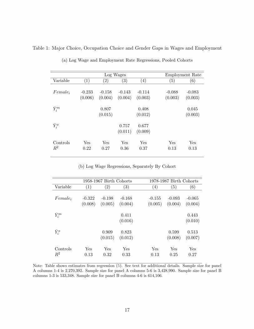
Table 1: Major Choice, Occupation Choice and Gender Gaps in Wages and Employment

(a) Log Wage and Employment Rate Regressions, Pooled Cohorts

Log Wages Employment Rate

Variable (1) (2) (3) (4) (5) (6)

Femalei -0.233 -0.158 -0.143 -0.114 -0.088 -0.083(0.006) (0.004) (0.004) (0.003) (0.003) (0.003)

Y mi 0.807 0.408 0.045

(0.015) (0.012) (0.003)

Y oi 0.757 0.677

(0.011) (0.009)

Controls Yes Yes Yes Yes Yes YesR2 0.22 0.27 0.36 0.37 0.13 0.13

(b) Log Wage Regressions, Separately By Cohort

1958-1967 Birth Cohorts 1978-1987 Birth Cohorts

Variable (1) (2) (3) (4) (5) (6)

Femalei -0.322 -0.198 -0.168 -0.155 -0.093 -0.065(0.008) (0.005) (0.004) (0.005) (0.004) (0.004)

Y mi 0.411 0.443

(0.016) (0.010)

Y oi 0.909 0.823 0.599 0.513

(0.015) (0.012) (0.008) (0.007)

Controls Yes Yes Yes Yes Yes YesR2 0.13 0.32 0.33 0.13 0.25 0.27

Note: Table shows estimates from regression (5). See text for additional details. Sample size for panelA columns 1-4 is 2,270,392. Sample size for panel A columns 5-6 is 3,428,990. Sample size for panel Bcolumns 1-3 is 533,348. Sample size for panel B columns 4-6 is 614,106.

17

Column 2 includes a control for the individual’s undergraduate major (as measured by Y mi ).

Column 3 includes a control for the individual’s current occupation (as measured by Y oi ).

Column 4 includes both the controls for undergraduate major and current occupation. Con-

trolling for major choice (but not occupation choice) reduces the gender gap in wages by

about one-third (to 15.9 log points). Controlling for occupation choice (but not major choice)

reduces the gender gap by 40 percent (to 14.4 log points). The key finding from Table 1

arises by comparing the results between columns 3 and 4. Controlling for undergraduate

major in addition to controlling for current occupation reduces the gender wage gap further

by an additional 2.8 percentage points. There is information in undergraduate major that

helps to explain gender differences in wage above and beyond current occupational choice.19

Collectively, controlling for occupation and undergraduate major reduces the gender wage

gap for college-educated women by half (11.5 log points).

Columns 5 and 6 of Table 1 evaluates the relationship between major choice and the

gender gap in extensive margin labor market participation. In the 2014-2017 ACS, highly

educated women were 8.6 percentage points less likely to work than men conditional on

demographics (column 5). As seen in column 6, controlling for major choice did not alter

the estimated gender gap in employment rates for women with a bachelor’s degree. This

specification cannot control for occupational choice given that occupation is often not defined

for those who are not working.20 While controlling for undergraduate major choice reduces

the estimated wage gap between college-educated men and women, major choice is not

important for understanding gender differences in employment rates for this group.

The bottom panel of Table 1 displays estimates from (5) when the sample is restricted

to include only those born between 1958-1967 (columns 1-3) and only those born between

1978-1987 (columns 4-6).21 For this panel, we only show results where the dependent variable

is log wages. Columns 1 and 4 show the gender wage gaps conditional on demographics for

the two cohorts. Columns 2 and 5 add controls for occupational choice. Columns 3 and

6 add controls for both occupational choice and major choice. The gender gap in wages

conditional on demographics fell from -32 log points to -16 log points between the 1958

and 1987 birth cohorts of college graduates. For each cohort separately, controlling for

is nearly identical to the estimated gender wage gap for young college graduates using historical U.S. Censusdata spanning the same cohorts. See the Online Appendix for additional details.

19These findings are complementary with the results in Brown and Corcoran (1997) which finds that majorchoice has predictive power in explaining gender wage gaps independent of occupation choice in cohorts bornin the 1940s and 1950s.

20Occupation is recorded for those who are not working only if they were employed at some point in theprior five years.

21To increase power in these regressions, we pool together adjacent 5-year cohorts to make 10-year cohorts.The Online Appendix shows similar regressions for all the 10-year cohorts in our data.

18

occupation and major reduces the gender wage gap by between 50 and 60 percent. This is

similar to the pooled cohort results in the top panel of the table. Also, within each cohort,

undergraduate major choice has predictive power above and beyond controlling just for

occupational choice. Interestingly, major choice has more predictive power and occupational

choice has less predictive power for more recent cohorts relative to older cohorts.

The bottom panel of Table 1 also allows us to assess how controlling for occupational

choice and undergraduate major alters the time series patterns in the gender wage gaps. By

comparing columns 1 and 4, the baseline gender wage gap fell by 18 percentage points for

a sample of individuals with a bachelors degree between cohorts born in the 1960s relative

to the 1980s. The gender wage gap after controlling for both occupational choice and major

choice fell by 11 percentage points. Therefore, the changing gender difference in both occu-

pational and major choice explain roughly 39 percent of the declining gender gap between

these two birth cohorts (1− 11/18).

Panel B of Table 1 provides evidence of large convergence in the college gender wage gap

across 10-year birth cohorts. In order to shed light on the power of our explanatory variables

within cohort, we conduct a wage decomposition exercise. We report the formal results in

Appendix Table A5 of the Online Appendix and briefly discuss those results here. Across

all 10-year birth cohorts, occupational specialization explains the largest share of the gender

wage gap for college graduates ranging from explaining 43.9% of the gap in the oldest cohort

(1948-1957) to explaining 36.9% of the gender wage gap in the youngest cohort (1978-1987).

Pre-labor market human capital specialization (major choice) is also important in explaining

the college gender wage gap ranging from explaining 17.6% of the gender wage gap in the

oldest cohort (1948-1957) to 27.9% of the gender wage gap in the youngest cohort (1978-

1987). Notably, human capital attainment above and beyond a bachelors degree (such as

a graduate degree) explains considerably less of the college gender wage gap. Occupational

specialization has become slightly less important over time; it explains about 7 percentage

points less of the gender wage gap in the youngest (1978-1987) compared to the oldest

(1948-1957) birth cohort. In contrast, college major has become increasingly important in

explaining the gender wage gap for college graduates over time; it explains 10.3 percentage

points more of the gap in the youngest (1978-1987) compared to the oldest (1948-1957) birth

cohort. These results suggest that properly accounting for human capital decisions above

and beyond schooling attainment and occupational specialization is centrally important in

understanding the causes of the gender wage gap among the highly-skilled.

19

6 Discussion and Conclusion

In this paper, we document five novel facts: (1) Over the past 40 years, men and women

have chosen more similar undergraduate majors. (2) Women have historically chosen college

majors associated with lower potential wages than men. Although these gaps have narrowed

over time, this is still true for women in the youngest birth cohorts. (3) There are gender

differences in the mapping of major to occupation. Women systematically choose lower

potential wage and lower potential hours-worked occupations than men even conditional on

major. (4) There is a modest convergence between the 1950 and 1990 birth cohorts in the

gendered mapping of major to occupation. (5) College major choice has strong predictive

power in explaining gender wage gaps independent of occupation choice. These trends arise

in an era where both labor force participation of women and the fraction of women that

have graduated from universities has increased dramatically, fundamentally changing the

composition of the educated workforce.

Attempts to measure detailed differences in pre-market specialization by college workers

have been limited by data availability. Researchers have long suspected that pre-market

specialization (major choice) should in some way pre-determine labor market opportunities

particularly with respect to occupational choice. As specialized knowledge is iterative, a

biochemical engineer would likely be ill-served by choosing studio art as her primary un-

dergraduate major. If men and women sort into field of study in systematically different

patterns, it follows that major choice should have non-trivial implications for the college

gender wage gap. The combined results of this paper support this intuition and underscore

the importance of further evaluating gender differences in pre-labor market specialization

including college major choice.

As a final thought, this work focuses on one aspect of pre-market specialization– major

choice. Yet, there are other ways in which men and women make pre-market investments

in human capital that pre-determine labor market opportunities. The results in this paper

suggest that an investigation into other avenues of pre-market specialization are important,

particularly investments that may happen earlier in the human capital chain. Further, un-

derstanding the mechanisms for gendered specialization– whether it is driven by preferences

or information- is of first-order concern for researchers.

20

References

Altonji, J.G., P. Arcidiacono, and A. Maurel, “Chapter 7 - The Analysis of FieldChoice in College and Graduate School: Determinants and Wage Effects,” in Eric A.Hanushek, Stephen Machin, and Ludger Woessmann, eds., Eric A. Hanushek, StephenMachin, and Ludger Woessmann, eds., Vol. 5 of Handbook of the Economics of Education,Elsevier, 2016, pp. 305 – 396.

Altonji, Joseph G and Rebecca M Blank, “Race and gender in the labor market,”Handbook of labor economics, 1999, 3, 3143–3259.

Altonji, Joseph G., Lisa B. Kahn, and Jamin D. Speer, “Trends in Earnings Differen-tials across College Majors and the Changing Task Composition of Jobs,” The AmericanEconomic Review, 2014, 104 (5), 387–393.

Bayard, Kimberly, Judith Hellerstein, David Neumark, and Kenneth Troske,“New evidence on sex segregation and sex differences in wages from matched employee-employer data,” Journal of labor Economics, 2003, 21 (4), 887–922.

Becker, Gary S, William HJ Hubbard, and Kevin M Murphy, “Explaining theworldwide boom in higher education of women,” Journal of Human Capital, 2010, 4 (3),203–241.

Bertrand, Marianne and Kevin F Hallock, “The gender gap in top corporate jobs,”ILR Review, 2001, 55 (1), 3–21.

Black, Dan, Amelia Haviland, Seth Sanders, and Lowell Taylor, “Gender WageDisparities Among the Highly Educated,” The Journal of Human Resources, 2008, 43 (3),630–59.

Black, Sandra E and Chinhui Juhn, “The rise of female professionals: Are womenresponding to skill demand?,” American Economic Review, 2000, 90 (2), 450–455.

Blau, Francine D and Lawrence M Kahn, “Swimming upstream: Trends in the genderwage differential in the 1980s,” Journal of labor Economics, 1997, 15 (1, Part 1), 1–42.

and , “Gender differences in pay,” Journal of Economic perspectives, 2000, 14 (4),75–99.

Blau, Francine D. and Lawrence M. Kahn, “The Gender Wage Gap: Extent, Trends,and Explanations,” Journal of Economic Literature, September 2017, 55 (3), 789–865.

, Marianne Ferber, and Anne Winkler, The Economics of Women, Men and Work,Pearson, 2014.

Blau, Francine D, Patricia Simpson, and Deborah Anderson, “Continuing progress?Trends in occupational segregation in the United States over the 1970s and 1980s,” Fem-inist economics, 1998, 4 (3), 29–71.

21

Brown, Charles and Mary Corcoran, “Sex-Based Differences in School Content and theMale-Female Wage Gap,” Journal of Labor Economics, 1997, 15 (3), 431–465.

Ceci, Stephen, Donna Ginther, Shulamit Kahn, and Wendy Williams, “Women inAcademic Science: A Changing Landscape,” Psychological Science in the Public Interest,2014, 15 (3), 75–141.

Charles, Kerwin Kofi and Ming-Ching Luoh, “Gender differences in completed school-ing,” Review of Economics and statistics, 2003, 85 (3), 559–577.

Cortes, Patricia and Jessica Pan, “Occupation and gender,” The Oxford Handbook ofWomen and the Economy, 2018, p. 425.

Cortez, Patricia and Jessica Pan, “Prevalence of Long Hours and Skilled Women’sOccupational Choice,” IZA Discussion Paper 10225, 2016.

Dickson, Lisa, “Race and Gender Differences in College Major Choice,” The Annals of theAmerican Academy of Political and Social Science, 2010, 627 (1), 108–124.

DiPrete, Thomas A and Claudia Buchmann, “Gender-specific trends in the value ofeducation and the emerging gender gap in college completion,” Demography, 2006, 43 (1),1–24.

Duncan, Otis Dudley and Beverly Duncan, “A Methodological Analysis of SegregationIndexes,” American Sociological Review, 1955, 20 (2), 210–217.

England, Paula and Su Li, “Desegregation Stalled: The Changing Gender Compositionof College Majors, 1971-2002,” Gender and Society, 2006, 20 (5), 657–676.

Goldin, Claudia, “Understanding the gender gap: An economic history of Americanwomen,” OUP Catalogue, 1992.

and Lawrence F. Katz, “The Cost of Workplace Flexibility for High-Powered Profes-sionals,” The Annals of the American Academy of Political and Social Science, 2011, 638(1), 45–67.

, , and Ilyana Kuziemko, “The Homecoming of American College Women: TheReversal of the College Gender Gap,” Journal of Economic Perspectives, 2006, 20 (4),133–156.

Groshen, Erica L et al., The structure of the female/male wage differential: Is it who youare, what you do, or where you work?, Vol. 44, Federal Reserve Bank of Cleveland, 1987.

Hsieh, Chang-Tai, Erik Hurst, Chad Jones, and Pete Klenow, “The Allocation ofTalent and Economic Growth,” Econometrica, 2019, forthcoming.

Jacob, Brian A, “Where the boys aren’t: Non-cognitive skills, returns to school and thegender gap in higher education,” Economics of Education review, 2002, 21 (6), 589–598.

22

Jacobsen, Joyce P, James Wishart Pearce III, and Joshua L Rosenbloom, “TheEffects of Childbearing on Married Women’s Labor Supply and Earnings.,” Journal ofHuman Resources, 1999, 34 (3).

Leslie, Larry L., Gregory T. McClure, and Ronald L. Oaxaca, “Women and Mi-norities in Science and Engineering: A Life Sequence Analysis,” The Journal of HigherEducation, 1998, 69 (3), 239–76.

Loury, Linda Datcher, “The Gender Earnings Gap among College-Educated Workers,”Industrial and Labor Relations Review, 1997, 50 (4), 580–593.

Macpherson, David A and Barry T Hirsch, “Wages and gender composition: why dowomen’s jobs pay less?,” Journal of labor Economics, 1995, 13 (3), 426–471.

Pan, Jessica, “Gender segregation in occupations: The role of tipping and social interac-tions,” Journal of Labor Economics, 2015, 33 (2), 365–408.

Ruggles, Steven, Sarah Flood, Ronald Goeken, Josiah Grover, Erin Meyer, JosePacas, and Matthew Sobek, “IPUMS USA: Version 9.0 [dataset],” 2019.

Turner, Sarah E. and William G. Bowen, “Choice of Major: The Changing (Unchang-ing) Gender Gap,” Industrial and Labor Relations Review, 1999, 52 (2), 289–313.

Zafar, Basit, “College Major Choice and the Gender Gap,” Journal of Human Resources,2013, 48 (3), 545–95.

23

Online Appendix for “Gender Differences in College

Major Choice: Not for Publication”

A1 Data Description

A1.1 Main ACS Samples

Our analysis is conducted using the 2014 to 2017 American Community Survey (ACS).The sample is restricted to include those who are not living in institutional group quarters,were born in one of the 50 U.S. states, have attained at least four years of college completion,and are age 23 to 67. We construct 5-year birth cohorts centered around the reported birthcohort. For example, the 1965 birth cohort includes those born between 1963 and 1967(inclusive). When data for key demographic variables is missing, the ACS imputes valuesincluding age, sex, race, place of birth, educational attainment and undergraduate major.In the 2014 to 2017 ACS, 276,448 (2.2% of the 2014-2017 ACS) respondents have imputededucational attainment information and 196,379 respondents (1.6% of the 2014-2017 ACS)have imputed degree field information. We restrict our sample to include only those withnon-imputed age, sex, race, origin, educational attainment and undergraduate major fieldinformation. We use inverse probability weighting to correct for non-response. In doing so,we preserve the age, sex race, and state of birth joint distribution. In total, our analysissample of ACS respondents includes 1,718,330 individuals.

In our analysis, we proxy an hourly wage by dividing reported annual labor income by thereported usual hours the respondent worked in the previous year times the reported numberof weeks the respondent worked during the previous year. As the weeks worked variableis an intervalled variable in the 2014-2017 ACS, we assign the midpoint of the category asthe number of weeks worked. Nominal wages are converted to real 2018$. In all analysesincluding wages, we follow the conventional practices in the literature and restrict the sampleto a set of people with well-measured wages: those who are employed civilians (excludingthe self-employed) with non-missing annual labor income and strong attachment to the labormarket defined as usually working at least 30 hours a week for a minimum of 27 weeks in theprevious year. In calculating the potential wage indices by occupation and undergraduatemajor, we restrict the sample to white men in their peak wage years (ages 45 to 55) withwell-measured wages. All analyses use log wages.

We use the variables degfield, degfield2, degfieldd, and degfield2d in IPUMS to identifyboth broad and detailed majors. IPUMS provides 176 detailed major codes for the 2014 to2017 samples. In our analysis, we aggregate to 134 detailed major categories by subsum-ing very small major categories into larger categories. For example, we combined GeneralAgriculture, Soil Science, and Miscellaneous Agriculture into one detailed agricultural ma-jor. Similarly, we combine Mathematics, Actuarial Science, and Mathematics and ComputerScience into one detailed mathematics major. Our main analysis uses these detailed majorcategories. There are 29 broad major categories in our analysis. We use the broad major cat-egories to describe trends in Figure 1 and describe major-to-occupation mappings in Figure3.

24

Approximately 11 percent of the observations in our sample have dual majors. Ouranalysis requires a maximum of one major for each unit of observation. Thus, we assigna primary major to each person based on the maximum median potential wage in the twomajors (based on white men aged 43-57 as described above). This assignment process relieson the assumption that agents will present their highest-wage major as their primary majorin the labor market.

Figures A1 to A5 include a full listing of our detailed and broad major codes. Our datareplication kit provides the code for our combination of majors.

We use a balanced panel of detailed occupation codes based on the 1990 Occupationcodes and following the cross-walking strategy outlined by David Dorn which constructs apanel of 330 occupation codes.22 In our analysis, we aggregate to 251 detailed occupationcodes by subsuming very small occupation categories into larger categories. For people whoare employed, the ACS reports occupation based on primary occupation. For people whoare unemployed, the ACS reports occupation based on their most recent primary occupationin the last five years.

A2 Gender Differences in Wages and Employment Rates,

Historical U.S. Censuses

As way of background, we measure time series trends in gender wage and employment gapsfor young individuals using cross-sectional data from historical U.S. Censuses. We focuson cross-sections from the 1960, 1970, 1980, 1990, and 2000 U.S. Censuses as well as the2010-2012 American Community Surveys (pooled). Within these data sets, we define thewages of those with at least a bachelor’s degree similarly to our wage computation withinthe 2014-2017 ACS. Employment rates are measured as the individual currently working atleast 30 hours per week (full-time).

The solid line in Figure A6 shows the difference in log wages between young workingwomen and young working men with a bachelor’s degree at decadal intervals using thehistorical Census and recent ACS data. We define ”young” as individuals between the agesof 25 and 34. Given the decadal frequency and 10-year age range, each point on the linesin Figure A6 represents a different cohort of individuals. Young women with at least abachelor’s degree entering the labor market in 1960 (born between 1926 and 1935) earnedaverage hourly wages that were 31 log points lower than their male counterparts. The genderwage gap for those with a bachelor’s degree narrowed to 13 log points for the young cohortentering the labor market in 2010 (born between 1976 and 1985). The wage gap declinedmonotonically by a total of 18 log points for the cohorts entering the labor market between1960 and 2010 with most of the decline occurring for cohorts entering the labor marketbetween 1980 and 1990 (those born between 1956 and 1965). The results in Figure A6 showthat substantial gender wage convergence occurred within the highly selected sample of thosewho attained a bachelor’s degree.

The dashed line of Figure A6 shows gender convergence in full time employment ratesamong our sample of college graduates. We define full time employment as those individuals

22See https://www.ddorn.net/data.htm.

25

who report currently working at least 30 hours per week. Throughout all years, roughly 90percent of college-educated young men reported working full time. For women, only about35 percent of 25-34 year old female college graduates worked full time in 1960 – a genderemployment rate gap of 35 percentage points. By 2010, roughly 80 percent of young educatedwomen worked full time. For individuals with a bachelor’s degree, there was a strong increasein women’s wages and employment propensities relative to their male counterparts during thelast half century. One goal of the paper is to assess how changing differences in undergraduatemajor choice is associated with changing gender wage and employment gaps across cohorts.

A3 Construction of Potential Wage Indices

In Section 3, we define our potential wage index as:

IP,Mc =

∑Mm=1 s

mfemale,cY

mmale∑M

m=1 smmale,cY

mmale

− 1 (6)

In practice, we compute this index by running the following regression locally within5-year birth cohort c:

Y mmalei

= α + βFemalei + ΓXi + εi (7)

where Femalei is a dummy variable indicating whether the respondent i has self-reportedas female and Xi is a vector of demographic characteristics: race, state of birth, mastersattainment, doctorate attainment, and marital status. Our potential wage index, IP,Mc , isdefined as β from each local regression by 5-year birth cohort and therefore, measures thedifferential “potential” wage of women of cohort c given that the female distribution of majorchoice in a given cohort may differ from males in their cohort. The units of this index aredifferential potential log wage based on major choice. In computing the comparable indexfor occupation, we substitute detailed occupation code, o, for detailed major code, m.

A4 Robustness: Key Results

A4.1 Robustness Figure 2

In Figure 2 of the main text, we restrict the sample on which our gender similarity indices arebuilt to all individuals with reported majors (for IDD,M

c and IP,Mc ) or to all individuals withreported occupations (for IDD,O

c and IP,Oc ). Some individuals with reported majors are notworking during the 2014-2017 period. Likewise, some individuals with reported occupationsare not currently working (given the ACS asks occupations for people who are currently notworking but may have worked at some point in the prior 5 years). To see if including thosewho are currently not working bias our indices, we perform a robustness exercise by creatingthe respective indices restricted to a sample of individuals with strong attachment to thelabor market as defined throughout our analysis (civilians who are not self-employed andreport working for at least 30 hours a week for at least 27 weeks in the previous year). Theresults of this exercise are shown in Appendix Figure A7. The results in Appendix Figure

26

A7 are nearly identical to the results in Figure 2 of the main text. This suggests that ourresults are insensitive to whether we include individuals with strong attachment to the labormarket or all individuals when describing patterns of gender sorting in major (occupation)choice.

Another potential issue with the results in Figure 2 stems from the fact that the ACSonly asks undergraduate major in recent years (from 2009 to 2017). When we comparepatterns for different birth cohorts, we risk confounding cohort and age effects. It is unlikelythat this is problematic for our results about the convergence of undergraduate majors giventhat major is likely fixed over an individual’s life cycle. Occupations are not fixed overthe lifecycle, so this presents a potential problem with respect to how we have describedoccupational segregation by gender in Figure 2. To address this and separate age and cohorteffects on occupational segregation by gender, we use data from the 1980, 1990, and 2000U.S. Censuses along with multiple waves of the American Community Survey to measureIDD,Oc for different birth cohorts at a constant age. The results are shown in Appendix Table

A1. As with the results in the main text, birth cohort refers to 5-year birth cohorts centeredaround the birth year listed. Similarly, age refers to 5-year age ranges centered on the agelisted. As seen in Appendix Table A1, age effects are not substantively biasing the mainresults shown in Figure 2 of the main text. Within each age range, we see large convergencein the occupation similarity between men and women across birth cohorts.

A4.2 Robustness Table 1, Panel A

Appendix Tables A2 and A3 show a series of robustness checks on the results shown in PanelA of Table 1 of the main text. Appendix Table A2 shows our key regression results withoutincluding our vector of demographic and time controls. Focusing on column 1 of the Table,the raw gender gap in wages among individuals without a bachelor’s degree for our pooledsample was 26.8 log points. Including demographic controls as in column 1 of Table 1 ofthe main text, the gender gap only fell to 23.3 log points. The demographic controls onlyexplain a small fraction of the gender wage gap among college graduates.

Appendix Table A3 shows the robustness results for Panel (a) of Figure 1 of the maintext to the alternate classification of majors and occupations. In our base specification in themain text, we used detailed occupation and major codes when defining the potential wagevariables Y m

i and Y oi . In the top panel of Appendix Table A3, we use the broad occupation

and major codes to define Y mi and Y o

i . In the bottom panel, we omit Y mi and Y o

i altogetherfrom the regression and instead include a vector of dummy variables for each broad major(occupation). The results of these alternate specifications are nearly identical to the resultsshown in Table 1 of the main text. This suggests that most of the variation in explaininggender wage gaps arises from differences across (as opposed to within) the broad major andoccupation controls.

A4.3 Table 1, Panel B

In Panel B of Table 1, we show the importance of occupational choice and undergraduatemajor in explaining gender wage gaps for the 1958-1967 and the 1978-1987 birth cohorts.Appendix Table A4 shows the same results for the 1948-1957 and the 1968-1977 birth cohorts.

27

A5 Hours Differences Across Occupations

As discussed in the main text, there is a large literature highlighting the fact that women arein occupations with lower annual hours worked relative to men. In this section, we explorethese results in the context of our methodology. To guide our empirical work, we define thefollowing two variables: Hm

male and Homale. H

mmale is defined as the median log annual hours

worked for native-born white men between the ages of 43 and 57 who graduated with majorm (regardless of subsequent occupation in which they worked). This is the potential hoursassociated with a given major based on older male hours. Ho

male is defined as the medianlog annual hours worked for native-born, white men between the ages of 43 and 57 whocurrently work in occupation o (regardless of undergraduate major). This is the potentialhours associated with a given occupation based on older male hours. We refer to thesevariables as our potential annual hours worked indices. Majors (occupations) where menwork more on average will have higher levels of Hm

male (Homale).

How similar are men and women with respect to their occupational choices based onpotential annual hours worked? Appendix Figure A8 displays IH,M

c and IH,Oc for different

cohorts. IH,Mc is our potential hours index based on male annual hours worked in different

majors and is defined as IH,Mc =

∑Mm=1 s

mfemale,cH

mmale∑M

m=1 smmale,cH

mmale

− 1. Like our potential wage indices in

the main text, the only reason IH,Mc only differs from 0 if men and women inhabit different

majors. Likewise, IH,Oc is our potential hours index based on male annual hours worked in

different occupations and is defined as IH,Oc =

∑Oo=1 s

mfemale,cH

omale∑O

o=1 smmale,cH

omale

− 1.

As seen from Appendix Figure A8, women choose majors and occupations associatedwith lower potential annual hours worked. The major and occupational choice of womenhave converged to that of men over time in a way that implies women and men are choosingmajors and occupations with more similar hours requirements. For the most recent cohorts,women are choosing both majors and occupations where potential annual hours worked areroughly 2% lower than men. Consistent with the literature, we find that college-educatedwomen are choosing occupations with lower annual hours worked. We contribute to the hoursliterature by introducing the fact that college-educated women are choosing undergraduatemajors associated with lower annual hours worked. We also show that the gender similarityof occupations and majors based on potential hours has been converging over time.

Appendix Figure A9 shows gender differences in the mapping of majors to occupationswhere we measure occupations in units of potential annual hours worked Ho

male. AppendixFigure A9 is otherwise analogous to Figure 3 of the main text. To measure gender differencesin occupational choice in hours units conditional on undergraduate major, we define IH,O

c |mwhich just recalculates IH,O

c (as defined above) restricting the sample to those individualsthat chose major m. Consider individuals who choose to major in engineering (Panel A, solidline). Women from the 1950 birth cohort who majored in engineering subsequently choseoccupations that had potential hours worked that were 2% lower than otherwise similarmales. That gap disappeared for women who majored in engineering after the 1975 birthcohort. For all majors, the gender gap in potential annual hours worked of occupationalchoice conditional on major has fallen over time. Women are now choosing occupations thatare more similar in hours worked to men, conditional on occupational choice.

28

Appendix Figure A10 summarizes the mapping of majors to occupations where we mea-sure occupations in potential hours space. This figure is otherwise analogous to Figure 4 inthe main text. Women from the 1975 birth cohort are in occupations – conditional on majorchoice – that have annual hours worked that are three percent lower than comparable men.As a reminder, occupational potential wage differences, conditional on major choice, wereabout 9 percent for this cohort. Some of the reason that women may be choosing occupationswith lower wages is that those occupations also have lower annual hours worked.

A6 Wage Gap Decompositions

In this section, we discuss the findings of a decomposition exercise where we assess thecontribution of the independent variables in our main estimation to the college gender wagegap. As with the estimations in Table 1 and Table A4, the sample is restricted to includethose with strong attachment to the labor market. We begin by estimating locally withinbirth cohort log wage equations for men only where race, state of residence, and maritalstatus are categorical variables. As with all other specifications, the independent variablefor Major is the potential log wage from major choice, Y m

i , and the independent variable forOccupation is the potential log wage from occupation choice, Y o

i . Entries in the ”Log Points”column are the within-cohort male − female differences in the mean of the correspondingvariable multiplied by the within-cohort male log wage coefficients of the correspondingvariable. Entries in the ”% Explained” column are the ”Log Points” entries divided by thewithin-cohort Total Raw Gap.

In our model specification, occupational specialization plays the largest role in explainingthe college gender wage gap. This is true for all 10-year birth cohorts. In the oldest birthcohort (1948-1957), occupation explains 43.9% of the gender wage gap. For the youngestbirth cohort (1978-1987), the importance of occupation declines by 7 percentage pointsexplaining 36.9% of the gender wage gap.

The results in Table 1 and Table A4 show that major choice and occupation choice areindependently related to the college gender wage gap. This finding is a contribution to theliterature on the college gender wage gap and the role of pre-market specialization. In ourdecomposition exercise, we formally show that pre-labor market human capital specialization(major choice) has non-trivial importance in explaining the college gender wage gap. Forthe oldest birth cohort (1948-1957), major choice explains 17.6% of the college gender wagegap. For the youngest birth cohort (1978-1987), major choice explains 27.9% of the collegegender wage gap. While much of the existing literature has focused on the role of humancapital attainment with respect to the gender wage gap, our decomposition shows that humancapital attainment above and beyond a bachelors degree (such as a graduate degree) explainsconsiderably less of the college gender wage gap than both pre-market and market humancapital specialization.

Finally, in thinking about the time series patterns, two findings are of particular inter-est. First, occupational specialization has become less important between the 1948-1957 and1958-1967 birth cohorts and then mostly stabilized. For the 1948-1957 birth cohort, occu-pation explained 43.9% of the college gender wage gap. This fell to 38.0% for the 1958-1967birth and was 37.5% and 36.9% for the 1968-1977 and 1978-1987 birth cohorts respectively.

29

Second, college major has become increasingly important in explaining the gender wage gapfor college graduates over time. It explained 10.3 percentage points more of the gap in theyoungest (1978-1987) compared to the oldest (1948-1957) birth cohort.

30

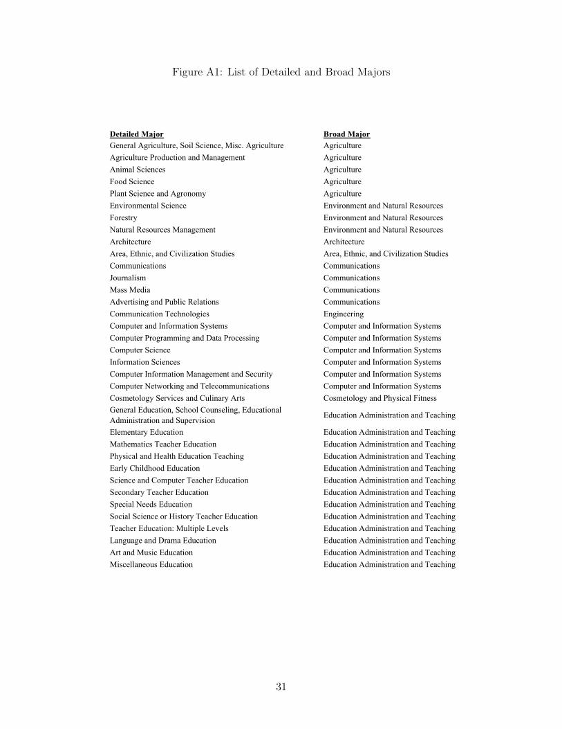
Figure A1: List of Detailed and Broad Majors

Detailed Major Broad MajorGeneral Agriculture, Soil Science, Misc. Agriculture AgricultureAgriculture Production and Management AgricultureAnimal Sciences AgricultureFood Science AgriculturePlant Science and Agronomy AgricultureEnvironmental Science Environment and Natural ResourcesForestry Environment and Natural ResourcesNatural Resources Management Environment and Natural ResourcesArchitecture ArchitectureArea, Ethnic, and Civilization Studies Area, Ethnic, and Civilization StudiesCommunications CommunicationsJournalism CommunicationsMass Media CommunicationsAdvertising and Public Relations CommunicationsCommunication Technologies EngineeringComputer and Information Systems Computer and Information SystemsComputer Programming and Data Processing Computer and Information SystemsComputer Science Computer and Information SystemsInformation Sciences Computer and Information SystemsComputer Information Management and Security Computer and Information SystemsComputer Networking and Telecommunications Computer and Information SystemsCosmetology Services and Culinary Arts Cosmetology and Physical FitnessGeneral Education, School Counseling, Educational Administration and Supervision Education Administration and Teaching

Elementary Education Education Administration and TeachingMathematics Teacher Education Education Administration and TeachingPhysical and Health Education Teaching Education Administration and TeachingEarly Childhood Education Education Administration and TeachingScience and Computer Teacher Education Education Administration and TeachingSecondary Teacher Education Education Administration and TeachingSpecial Needs Education Education Administration and TeachingSocial Science or History Teacher Education Education Administration and TeachingTeacher Education: Multiple Levels Education Administration and TeachingLanguage and Drama Education Education Administration and TeachingArt and Music Education Education Administration and TeachingMiscellaneous Education Education Administration and Teaching

31

Figure A2: List of Detailed and Broad Majors (continued)

Detailed Major Broad Major

Engineering: General, Military Technologies, Metallurgical, Biomedical, Geological and Geophysical, Mining and Mineral, Naval Architecture and Marine, Nuclear, Petroleum

Engineering

Aerospace Engineering EngineeringBiological Engineering EngineeringChemical Engineering EngineeringCivil and Architectural Engineering EngineeringComputer Engineering Engineering

Electrical Engineering, Electrical Engineering Technology, Electrical and Mechanic Repairs and Technologies Engineering

Engineering Mechanics, Physics, and Science EngineeringEnvironmental Engineering EngineeringIndustrial and Manufacturing Engineering, Precision Production and Industrial Arts Engineering

Mechanical Engineering EngineeringMiscellaneous Engineering EngineeringEngineering Technologies EngineeringEngineering and Industrial Management EngineeringIndustrial Production Technologies EngineeringMechanical Engineering Related Technologies EngineeringMiscellaneous Engineering Technologies EngineeringLinguistics, and Comparative Language and Literature Linguistics and Foreign Languages

French, German, Latin and Other Common Foreign Languages Linguistics and Foreign Languages

Other Foreign Languages Linguistics and Foreign LanguagesFamily and Consumer Sciences Family and Consumer SciencesPre-Law and Legal Studies, Court Reporting LawEnglish Language and Literature English and LiteratureComposition and Speech English and LiteratureLiberal Arts Liberal Arts and HumanitiesHumanities Liberal Arts and HumanitiesLibrary Science Education

32

Figure A3: List of Detailed and Broad Majors (continued)

Detailed Major Broad MajorBiology, Misc. Biology, Pharmacology, Botany, Neuroscience, Genetics Biology and Life Sciences

Biochemical Sciences Biology and Life SciencesMolecular Biology Biology and Life SciencesEcology Biology and Life SciencesMicrobiology Biology and Life SciencesPhysiology Biology and Life SciencesZoology Biology and Life SciencesMathematics, Actuarial Science, Mathematics and Computer Science Math and Statistics

Applied Mathematics Math and StatisticsStatistics and Decision Science Math and StatisticsInterdisciplinary,Multi-Disciplinary, Intercultural and International Studies Multi-Disciplinary Studies (General)

Nutrition Sciences Multi-Disciplinary Studies (General)Physical Fitness, Parks, Recreation, and Leisure Cosmetology and Physical FitnessPhilosophy and Religious Studies Philosophy and TheologyTheology and Religious Vocations Philosophy and Theology

Physical Sciences, Astronomy and Astrophysics, Geosciences, Nuclear, Industrial Radiology, and Biological Technologies Physical Sciences

Atmospheric Sciences and Meteorology Physical SciencesChemistry Physical SciencesGeology and Earth Science Physical SciencesOceanography Physical SciencesPhysics Physical SciencesMaterials Science and Materials Engineering EngineeringMulti-disciplinary or General Science Physical SciencesPsychology, Cognitive Science and Biopsychology, Social Psychology Psychology

Educational Psychology PsychologyClinical Psychology PsychologyCounseling Psychology PsychologyIndustrial and Organizational Psychology PsychologyMiscellaneous Psychology Psychology

33

Figure A4: List of Detailed and Broad Majors (continued)

Detailed Major Broad MajorCriminal Justice and Fire Protection Criminal Justice and Fire ProtectionPublic Administration Public Affairs, Policy, and Social WorkPublic Policy Public Affairs, Policy, and Social WorkHuman Services and Community Organization Public Affairs, Policy, and Social WorkSocial Work Public Affairs, Policy, and Social WorkGeneral Social Sciences Social Sciences

Economics, Agricultural Economics, Business Economics Social Sciences

Anthropology and Archeology Social Sciences Criminology Social Sciences Geography Social Sciences International Relations Social Sciences Political Science and Government Social Sciences Sociology Social Sciences Miscellaneous Social Sciences Social Sciences Construction Services Construction ServicesTransportation Sciences and Technologies Construction Services

Fine Arts, Commercial Art and Graphic Design, Film, Video and Photographic Arts, Studio Arts, Miscellaneous Fine Arts Fine Arts

Drama and Theater Arts, Music, Visual and Performing Arts Fine Arts

Art History and Criticism Fine ArtsGeneral Medical and Health Services Nursing, Medical and Health SciencesCommunication Disorders Sciences and Services Nursing, Medical and Health SciencesHealth and Medical Administrative Services Nursing, Medical and Health SciencesMedical Assisting Services Nursing, Medical and Health SciencesMedical Technologies Technicians Nursing, Medical and Health SciencesHealth and Medical Preparatory Programs Nursing, Medical and Health SciencesNursing Nursing, Medical and Health SciencesPharmacy, Pharmaceutical Sciences, and Administration Nursing, Medical and Health SciencesTreatment Therapy Professions Nursing, Medical and Health SciencesCommunity and Public Health Nursing, Medical and Health SciencesMiscellaneous Health Medical Professions Nursing, Medical and Health Sciences

34

Figure A5: List of Detailed and Broad Majors (continued)

Detailed Major Broad MajorGeneral Business BusinessAccounting BusinessBusiness Management and Administration BusinessOperations, Logistics and E-Commerce BusinessMarketing and Marketing Research BusinessFinance BusinessHuman Resources and Personnel Management BusinessInternational Business BusinessHospitality Management BusinessManagement Information Systems and Statistics BusinessMiscellaneous Business and Medical Administration BusinessHistory HistoryUnited States History History

35

Figure A6: Gender Differences in Log Wages and Employment Rates, Individuals Aged 25-34with Bachelor’s Degree

-0.60

-0.50

-0.40

-0.30

-0.20

-0.10

0.00

1960 1970 1980 1990 2000 2010

Gender Difference in EmploymentRate (Female vs. Male)

Gender Difference in Log Wages (Female vs. Male)

Notes: Figure shows the gender gap in log wages (solid line) and the gender gap in employmentrates (dashed line) for individuals aged 25-34 with a bachelor’s degree in different Census years.The 2010 data refers to a pooled sample of ACS respondents from sample years 2010, 2011, and2012. Individual wages are self-reported annual labor income divided by self-reported annualhours worked. The employment rate is the fraction of respondents who report working full-time.Differences are measured as female data minus male data. See text for additional details.

36

Figure A7: Gender Similarity in Major Choice and Occupation by Cohort, Strongly AttachedSample

0.44

0.48

0.52

0.56

0.60

0.64

0.68

0.72

0.76

1950 1955 1960 1965 1970 1975 1980 1985 1990

Inve

rse

Dun

can-

Dun

can

Segr

egat

ion

Inde

x

Five Year Birth Cohort

Major Occupation

-0.16

-0.15

-0.14

-0.13

-0.12

-0.11

-0.10

-0.09

-0.08

-0.07

1950 1955 1960 1965 1970 1975 1980 1985 1990

Pote

ntia

l Ln

Wag

e

Five Year Birth Cohort

Major Occupation

Panel A: Segregation Index Panel B: Potential WageIndex Index

Notes: Figure plots the inverse segregation index (left panel) and potential wage index (right panel) fordifferent cohorts conditioning on strong attachment to the labor market. The solid line in each panel showthe indices for major choice. The dashed line in each panel show the indices for occupation. Data from the2014-2017 ACS and is restricted to those with at least a bachelor’s degree. See text for additional details.

37

Figure A8: Gender Similarity in Major and Occupation by Cohort, Measuring Occupationsby Potential Hours Worked

-0.070

-0.060

-0.050

-0.040

-0.030

-0.020

-0.010

0.000

1950 1955 1960 1965 1970 1975 1980 1985 1990

Pote

ntia

l Ln

Ann

ual H

ours

Wor

ked

Five Year Birth Cohort

Major Occupation

Notes: Figure plots the gender similarity index for different cohorts based on potential hours worked. Thesolid line in each panel shows the indices based on major choice. The dashed line shows the indices based onsubsequent occupation. Data from the 2014-2017 ACS and is restricted to those with at least a bachelor’sdegree. See text for additional details.

38

Figure A9: Within-Major Gender Differences in Potential Hours by Occupation, by Genderand Cohort

-0.08

-0.06

-0.04

-0.02

0

0.02

1950 1955 1960 1965 1970 1975 1980 1985 1990

Fem

ale

-Mal

e M

ean

Pote

ntia

l Ln

Ann

ual H

ours

Wor

ked

Occ

upat

ion

Five Year Birth Cohort

Engineering Biology/Life Sciences Physical Sciences Business History

-0.08

-0.06

-0.04

-0.02

0

0.02

1950 1955 1960 1965 1970 1975 1980 1985 1990

Fem

ale

-Mal

e M

ean

Pote

ntia

l Ln

Ann

ual H

ours

Wor

ked

Occ

upat

ion

Five Year Birth Cohort

Education Psychology Fine Arts Nursing/Pharmacy Foreign Languages

Panel A: Male Dominated Panel B: Female DominatedMajors Majors

Notes: These figures show the trends in IH,O|mc conditional on having graduated with major m. Panel A are

male-dominated majors. Panel B are female-dominated majors. As with the left panel of Figure 2, potentialwage in an occupation, Ho

male, is computed using only annual hours worked of native white males 43-57 whoare working full time in the 2014-2017 ACS.

Figure A10: Mapping of Potential Wages by Major to Potential Hours by Occupation, byGender and Cohort

7.60

7.62

7.64

7.66

7.68

7.70

7.72

7.74

7.76

1 2 3 4 5 6 7 8 9 10

Mea

n Po

tent

ial L

n A

nnua

l Hou

rs W

orke

d O

ccup

atio

n

Bin Potential Ln Wages Major

1955 female 1955 male 1965 female 1965 male 1975 female 1975 male

-0.07

-0.06

-0.05

-0.04

-0.03

-0.02

-0.01

0

1 2 3 4 5 6 7 8 9 10

Fem

ale

-Mal

e L

n Po

tent

ial H

ours

Occ

upat

ion

Bin Potential Ln Wages Major

1955 Cohort 1975 Cohort

Panel A: Levels Panel B: Differences

Notes: These figures show the mapping between major and occupation. On the x-axes, we have binnedmajors based on Y m

male, the log wage deciles of native, white men age 43 to 57. On the y-axis in Panel A, we

report IH,O|d,mc , the mean log potential occupational hours worked within these deciles described separately

by gender and cohort. In Panel B, the y-axis reports female - male differences in IH,O|d,mc for two of the

cohorts.

39

Table A1: Robustness of Trends in Inverse Duncan-Duncan Index for Gender OccupationalSimilarity, Controlling for Age Effects

Cohort 30 35 40 45 50 55

1925 0.3581930 0.3681935 0.380 0.4391940 0.405 0.4751945 0.435 0.499 0.5171950 0.496 0.503 0.5171955 0.522 0.520 0.5511960 0.609 0.555 0.559 0.5761965 0.592 0.565 0.5831970 0.621 0.581 0.5821975 0.605 0.5911980 0.625 0.6071985 0.632

Note: This table computes the inverse Duncan-Duncan index forgender similarity in occupational sorting (IDD,O

c ) for differentbirth cohorts and age ranges. See main text for construction ofthe index. Cohorts are five year birth cohorts centered around thebirth cohort listed. Age are five year age ranges centered aroundthe age listed. Data come from the 1980, 1990, and 2000 U.S.Censuses as well as various years of the American CommunitySurvey.

40

Table A2: Major Choice, Occupation Choice and Gender Gaps in Wages and Employment

(a) Log Wage Regressions, No Controls

Log Wages Employment Rate

Variable (1) (2) (3) (4) (5) (6)

Femalei -0.268 -0.189 -0.160 -0.135 -0.075 -0.066(0.007) (0.006) (0.005) (0.004) (0.003) (0.003)

Y mi 0.827 0.355 0.091

(0.017) (0.014) (0.005)

Y oi 0.862 0.793

(0.011) (0.009)

Controls No No No No No NoR2 0.04 0.10 0.23 0.23 0.01 0.01

Note: This table is a robustness check on panel (a) of Table 1 with no demographic or time controls.Sample size for columns 1-4 is 2,270,392. Sample size for columns 5-6 is 3,428,990.

41

Table A3: Major Choice, Occupation Choice and Gender Gaps in Wages and Employment,Alternative Specifications Using Broad Major and Occupations

(a) Log Wage and Employment Rate Regressions with Broad Major and Occupation PotentialWage Indices, Pooled Cohorts

Log Wages Employment Rate

Variable (1) (2) (3) (4) (5) (6)

Femalei -0.232 -0.172 -0.167 -0.141 -0.088 -0.083(0.006) (0.004) (0.004) (0.004) (0.003) (0.003)

Y mi 0.832 0.461 0.061

(0.022) (0.015) (0.004)

Y oi 0.750 0.668

(0.013) (0.010)

Controls Yes Yes Yes Yes Yes YesR2 0.22 0.26 0.33 0.34 0.13 0.13

(b) Log Wage and Employment Rate Regressions with Flexible, Broad Major and OccupationDummies, Pooled Cohorts

Log Wages Employment Rate

Variable (1) (2) (3) (4) (5) (6)

Femalei -0.232 -0.169 -0.168 -0.143 -0.088 -0.083(0.006) (0.005) (0.004) (0.004) (0.003) (0.003)

Major dummies No Yes No Yes No YesOccupation dummies No No Yes Yes No NoControls Yes Yes Yes Yes Yes YesR2 0.22 0.27 0.34 0.35 0.13 0.13

Note: This table is a robustness check on the main results in Panel (a) of Table 1 using two alternateways to control for occupation and major choice. In Panel (a) of this table, we include as independentvariables measures of potential wages determined by the broad major and occupation choice instead ofdetailed major and occupation choice. In panel (b), we include as independent variables vectors of broadmajor dummies and occupation dummies instead of our potential wage controls. Sample size for panelA columns 1-4 is 2,256,630. Sample size for panel A columns 5-6 is 3,428,990. Sample size for panel Bcolumns 1-4 is 2,256,630. Sample size for panel B columns 5-6 is 3,428,990.

42

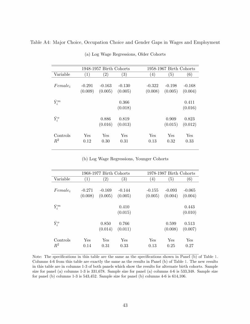
Table A4: Major Choice, Occupation Choice and Gender Gaps in Wages and Employment

(a) Log Wage Regressions, Older Cohorts

1948-1957 Birth Cohorts 1958-1967 Birth Cohorts

Variable (1) (2) (3) (4) (5) (6)

Femalei -0.291 -0.163 -0.130 -0.322 -0.198 -0.168(0.009) (0.005) (0.005) (0.008) (0.005) (0.004)

Y mi 0.366 0.411

(0.018) (0.016)

Y oi 0.886 0.819 0.909 0.823

(0.016) (0.013) (0.015) (0.012)

Controls Yes Yes Yes Yes Yes YesR2 0.12 0.30 0.31 0.13 0.32 0.33

(b) Log Wage Regressions, Younger Cohorts

1968-1977 Birth Cohorts 1978-1987 Birth Cohorts

Variable (1) (2) (3) (4) (5) (6)

Femalei -0.271 -0.169 -0.144 -0.155 -0.093 -0.065(0.008) (0.005) (0.005) (0.005) (0.004) (0.004)

Y mi 0.410 0.443

(0.015) (0.010)

Y oi 0.850 0.766 0.599 0.513

(0.014) (0.011) (0.008) (0.007)

Controls Yes Yes Yes Yes Yes YesR2 0.14 0.31 0.33 0.13 0.25 0.27

Note: The specifications in this table are the same as the specifications shown in Panel (b) of Table 1.Columns 4-6 from this table are exactly the same as the results in Panel (b) of Table 1. The new resultsin this table are in columns 1-3 of both panels which show the results for alternate birth cohorts. Samplesize for panel (a) columns 1-3 is 331,678. Sample size for panel (a) columns 4-6 is 533,348. Sample sizefor panel (b) columns 1-3 is 543,452. Sample size for panel (b) columns 4-6 is 614,106.

43

Table A5: Wage Decompositions: Explanatory Variables

(a) Older Cohorts

1948-1957 Birth Cohort 1958-1967 Birth CohortVariable (Log Points) (% Explained) (Log Points) (% Explained)

Race 0.0008 0.25% 0.0011 0.32%State 0.0004 0.14% 0.0002 0.06%Marital Status 0.0287 9.19% 0.0164 4.74%Masters -0.0048 -1.55% -0.0034 -0.99%Doctorate 0.0056 1.80% 0.0022 0.63%Major 0.0549 17.57% 0.0547 15.81%Occupation 0.1371 43.86% 0.1314 37.97%Y ear -0.0006 -0.19% -0.0001 -0.04%Explained 0.2221 71.07% 0.2025 58.51%Unexplained 0.0904 28.93% 0.1436 41.49%Total Raw Gap 0.31 0.35

(b) Younger Cohorts

1968-1977 Birth Cohort 1978-1987 Birth CohortVariable (Log Points) (% Explained) (Log Points) (% Explained)

Race 0.0004 0.13% 0.0001 0.04%State 0.0001 0.03% 0.0001 0.05%Marital Status 0.0146 5.03% 0.0002 0.11%Masters -0.0080 -2.76% -0.0064 -4.09%Doctorate 0.0007 0.25% 0.0000 0.03%Major 0.0444 15.27% 0.0438 27.85%Occupation 0.1090 37.53% 0.0579 36.86%Y ear -0.0003 -0.09% 0.0001 0.03%Explained 0.1609 55.39% 0.0956 60.87%Unexplained 0.1296 44.61% -0.0615 39.13%Total Gap 0.29 0.16

Note: Sample restrictions and cohorts consistent with Table A4. In these estimations, race, state ofresidence, and marital status are categorical variables instead of flexible dummies. This does not affectour main results and is only for ease in decomposition and display. As with all other specifications, theindependent variable for Major is Y m

i , and the independent variable for Occupation is Y oi . Entries in the

”Log Points” column are the within-cohort male− female differences in the mean of the correspondingvariable multiplied by the within-cohort male log wage coefficients of the corresponding variable. Entriesin the ”% Explained” column are the ”Log Points” entries divided by the within-cohort Total Raw Gap.The Total Raw Gap differs from the Femalei in Column (1) of Table A4 in that it is the raw genderwage gap with no controls and the gender wage gap displayed as the coefficient for Femalei in Column(1) of Table A4 includes demographic controls.

44