Federal Reserve Bank of Dallas Globalization and Monetary Policy Institute

Working Paper No. 279 http://www.dallasfed.org/assets/documents/institute/wpapers/2016/0279.pdf

Trends and Cycles in Small Open Economies: Making

The Case For A General Equilibrium Approach*

Kan Chen BBVA Research

Mario Crucini

Vanderbilt University and NBER

August 2016

Abstract Economic research into the causes of business cycles in small open economies is almost always undertaken using a partial equilibrium model. This approach is characterized by two key assumptions. The first is that the world interest rate is unaffected by economic developments in the small open economy, an exogeneity assumption. The second assumption is that this exogenous interest rate combined with domestic productivity is sufficient to describe equilibrium choices. We demonstrate the failure of the second assumption by contrasting general and partial equilibrium approaches to the study of a cross-section of small open economies. In doing so, we provide a method for modeling small open economies in general equilibrium that is no more technically demanding than the small open economy approach while preserving much of the value of the general equilibrium approach. JEL codes: C55, C68, F41, F44

* Kan Chen, BBVA Research, 2200 Post Oak Blvd. Houston, TX 77056. Kan.chen@bbva.com. Mario Crucini, Department of Economics, Box 351819-B, Vanderbilt University, Nashville, TN 37235. 615-322-7357. mario.j.crucini@vanderbilt.edu. The views in this paper are those of the authors and do not necessarily reflect the views of the Federal Reserve Bank of Dallas or the Federal Reserve System.

1 Introduction

The veracity of business cycles differs dramatically across countries. Figure 1 presents a

comprehensive view: it displays the standard deviation of annual output and consumption

growth rates computed over the period 1971 to 2011 for 66 countries (countries are ranked

from the most to least volatile).1 The standard deviation of output growth ranges from an

astounding 24.3% in Iraq (not shown) to a mere 1.58% in Australia; the median country is

Luxembourg (3.53%). An important goal of quantitative business cycle theory is to explain

these differences.

In this respect, the work-horse small open economy model has considerable appeal be-

cause it is possible to treat the world interest rate as given (i.e. determined in the rest-of-the-

world), an exogeneity assumption and conduct a partial equilibrium analysis. Aguiar and

Gopinath (2007) is a recent leading example of this approach. They argue persuasively that

much of the cross-country heterogeneity in the veracity of business cycles is accounted for

by differences in the relative importance of permanent and transitory shocks to total factor

productivity. The logic is simple. A permanent shock leads to larger jump in consumption

than a persistent, but transitory, shock because it entails a larger wealth effect. Output, to

a reasonable first-approximation, follows the path of productivity and therefore inherits the

volatility and persistence properties of the shock itself. Altering the relative importance of

the two shocks therefore allows one to match the standard deviation of output and consump-

tion patterns displayed in Figure 1. Applying this method to 13 emerging and 13 developed

economies, Aguiar and Gopinath find that the permanent component accounts for 84% of

productivity growth for emerging markets compared to 61% for developed countries.2

The use of a partial equilibrium model comes at a cost however, as it fails to capture

any meaningful economic interactions across nations. The most obvious is the international

correlation of business cycles. To fill this gap, we revisit the study of AG, using the two-

country general equilibrium model developed by Baxter and Crucini (1995). The BC model

1The PWT 8.1 starts from 1951 and ends in 2011. The starting year of 1971 allows for a comprehensiveand balanced cross-country panel.

2Note, they do not report a variance decomposition of output growth in their paper, though productivityand output tend to move closely in neoclassical models of the business cycle.

2

is a natural choice because it shares virtually all features of preferences, technology and the

asset market structure of AG, while closing the model by imposing world market clearing

in the goods market and the market for one-period non-contingent bonds.

In our simulations, the ‘home’ country is parameterized to mimic the business cycle of

an aggregate of (listed in descending economic size) the United States, Japan, the United

Kingdom, Germany, Italy, France, Canada and Australia (hereafter the G-8). This massive

economic block effectively determines the world interest rate (marginal product of capital).

The ‘foreign’ country is one of the 58 economies in our panel dataset. Individual countries

are rotated through in separate model simulations to produce the entire cross-section of

business cycle implications that are consistent with the domestic and foreign business cycle

facts.

Total factor productivity in the G-8 is the sum of a pure random walk component and a

transitory but persistent component. Matching the standard deviation of: i) consumption

growth, ii) income growth and iii) the consumption-GDP ratio for the G-8 block yields an es-

timated standard deviation of 0.9% (1.2%) for the innovation to the permanent (transitory)

component. The persistence of the transitory component is 0.9. The implication of these

estimates is that the transitory component contributes 58% to the standard deviation of

TFP growth, compared to 42% for the stationary component. These estimates are broadly

consistent with the less structural approach of Crucini and Shintani (2015); they estimate

a bivariate error-correction model of output and consumption growth for each country of

the G-8 and find comparable contributions of stochastic trend and cycle shocks to output

growth.

For each country outside of the G-8, we match the standard deviation of output growth,

the standard deviation of consumption and the correlation of output and consumption

growth of each country with the output and consumption growth of the G-8 block. To

accomplish this – in addition to an idiosyncratic permanent and transitory shock to pro-

ductivity in each country – we allow for a spillover from the G-8 permanent and transitory

shock. The productivity spillovers from the G-8 is the point of departure from the partial

3

equilibrium approach and allows us to match international business cycle comovement of

consumption and output.3

On average (across countries), the permanent shocks account for 45% of output growth in

developing countries compared to 51% in developed countries. These results contrast sharply

with AG who attribute 84% of productivity growth to permanent shocks for emerging mar-

kets compared to 61% for developed countries. While there are a number of differences in

terms of the sample of countries and sample period, the main driver of the difference is our

general equilibrium approach and the additional empirical discipline of matching interna-

tional business cycle comovement. We demonstrate this in two ways.

First, we use a small open economy model to match national business cycle moments

(excluding international comovement) in our cross-section and find the permanent shocks

must account for twice as much of output growth for developing countries compared to

developed countries, which is even more skewed in the direction of AG’s earlier findings.

This demonstrates that our results using the same modeling approach as AG also imply

a dominant role for permanent shocks in developing countries. The even larger roll of the

permanent shock may be a consequence of the Great Recession.

Second, shocks to the exogenous interest rate play a non-trivial role, accounting for about

25% of output growth variation in the average country (both developing and developed).

Since the real interest rate is stationary in the model, it is impossible to determine the role

of permanent and transitory shocks in accounting for real interest rate fluctuations without

a general equilibrium model. To demonstrate the identification issue, when we incorporate

the international spillovers of productivity estimated from the general equilibrium model,

the real interest rate plays almost no role in the small open economy version despite the fact

that the small open economy with spillovers of productivity produces virtually the same

variance decomposition as the general equilibrium model with spillovers.

The lessons here are stark. The logical contradiction of the small open economy approach

is that any comovement of business cycles through productivity transmission (or endogenous

3Consistent with the partial equilibrium approach, there are no productivity spillovers from the smallcountries to the large countries: a block-exogeneity assumption.

4

propagation) must be attributed to domestic productivity or the “world” interest rate.

Any yet, the world interest rate is not determined by the business cycle of the small open

economy leading to a fundamental issue of identification and mis-specification of the variance

decomposition.

2 The one-sector stochastic growth model

Our use of the basic one-sector, two-country stochastic growth model is motivated by two

objectives. The first is to stay as close as possible to the model specification utilized by

AG. The second is to ensure that the general equilibrium and partial equilibrium versions of

the model are structurally compatible. Three sources of novelty are introduced into these

otherwise standard models. First, careful attention is given to international productivity

spillovers from the large G-8 block to each individual nation. Second, the cross-section of

countries is comprehensive. Third, general equilibrium and partial equilibrium models are

explicitly compared. The general equilibrium model is the one-sector, two country, DSGE

model developed by Baxter and Crucini (1995). The partial equilibrium version of this model

omits the world goods market clearing condition and adds a stochastic process to capture

the evolution of the world interest rate.4 This section begins by quickly reviewing common

features of these two versions of the one-sector model and concludes with a discussion of the

differences.

2.1 Preferences and technology

Individuals in each country have Cobb-Douglas preferences over consumption and leisure

U(Cjt, Ljt) = βt1

1− σ[CθjtL

1−θjt ]1−σ, (1)

where parameter θ ∈ (0, 1), and the inter-temporal elasticity of substitution is 1/σ.

4AG incorporate a domestic interest rate response to home debt relative to productivity, but this playsa minor quantitative role in their exercise.

5

The final good is produced using capital and labor. The production function is Cobb-

Douglas and each country experiences stochastic fluctuations in the level of factor produc-

tivity, Ajt,

Yjt = AjtK1−αjt Njt

α . (2)

The stochastic processes for productivity will involve both permanent and transitory com-

ponents each potentially with a component common G-8 (world) component and an idiosyn-

cratic or nation-specific component. These stochastic processes are described in more detail

below.

The capital stock in each country, depreciates at the rate δ and is costly to adjust:

Kjt+1 = (1− δ)Kjt + φ(Ijt/Kjt)Kjt, (3)

where φ(·) is the adjustment cost function. As in Baxter and Crucini (1995), adjustment

costs have the following properties: i) at the steady-state, φ(I/K) = I/K and φ′(I/K) =

1 so that in the deterministic solution to the model the steady state with and without

adjustment costs are the same and ii) φ′ > 0, φ′′ < 0.

2.2 Closing the model

Following Baxter and Crucini (1995), the two country general equilibrium model is closed

by imposing one intertemporal budget constraint and world goods market clearing. The

intertemporal budget constraint is:

PBt Bjt+1 −Bjt = Yjt − Cjt − Ijt (4)

where Bjt+1 denotes the quantity of bonds purchased in period t by country j. PBt is the

price of a bond purchased in period t and maturing in period t+ 1. The bond is not state-

contingent, it pays one physical unit of consumption in all states of the world. Implicitly

this defines, rt, the real rate of return for the bond (i.e., PBt ≡ (1 + rt)−1 < 1). The

6

price of this bond is endogenous in the two-country equilibrium model, determined by the

market-clearing condition in the world bond market.

The world goods market clearing condition is:

π0(Y0t − C0t − I0t) + πj(Yjt − Cjt − Ijt) = 0, (5)

where πj denotes the fraction of world GDP produced by country j. These weights are

necessary to define market clearing because the quantities in the constraint are in domestic

per capita terms.

The small open economy is closed with an inter-temporal budget constraint identical to

(4). However, the discount rate follows an exogenous stochastic process describe below. In

addition, the following boundary condition is imposed:

limt→∞

βtpjtBjt+1 = 0,

where pjt is the multiplier on the inter-temporal budget constraint of the representative

agent in country j.

Parameterization of tastes and technology are set to values commonly used in the liter-

ature. The value of β is set to be 0.954, so that the annual real interest rate is 6.5%. The

parameter of relative risk aversion σ is 2 and labor’s share α in the production function is

0.58. In the Cobb-Douglas preference function, θ = 0.233. The depreciation rate of capital,

δ, is assigned a value of 0.10. The elasticity of the investment-capital ratio with respect to

Tobin’s Q is η = −(φ′/φ′′)÷ (i/k) = 15.

2.3 Exogenous shocks

Moving from theory to quantitative implications requires estimation of the stochastic pro-

cess for productivity in each country. Partial equilibrium models require specification of

stochastic processes for home country productivity and the domestic interest rate. General

equilibrium models require the estimation of stochastic processes for both home and foreign

7

productivity since the interest rate is endogenous. Our specification and estimation method

for each of these stochastic processes is discussed in turn below.

2.3.1 Total factor productivity

Beginning with the G-8 aggregate, indexed by 0, the logarithm of productivity is the sum of

a non-stationary and a stationary component, lnA0t = lnAP0t+lnAT0t. The non-stationary

component follows a pure random walk,

lnAP0t = lnAP0t−1 + ln εP0t , (6)

and the stationary component follows an AR(1) process:

lnAT0t = ρ0 lnAT0t−1 + ln εT0t . (7)

The innovations are drawn from independent normal distributions with different standard

deviations: εT0t ∼ N(0, σT0 ), εP0t ∼ N(0, σP0 ).

As the G-8 is by far the largest region and we assume that productivity spillovers are from

the G-8 to each nation of the G-60 and not the reverse. Simulations of the closed economy

version of the benchmark model are used to estimate the parameters of the productivity

components of the G-8 (effectively this involves setting π = 1 in the general equilibrium

model described earlier). Inputs into the estimation are G-8 aggregates, constructed as

country-size-weighted averages of output growth, consumption growth and the logarithm of

the consumption-output ratio.

Productivity parameters are chosen to match the observed sample variances of these three

key macroeconomic variables. The outcome of the moment-matching exercise is reported

in Table 1. The average difference (across countries) between the moments from the data

and from the model simulation, reported in the upper panel of the table, is less than 10%

in all cases. The estimated persistence of the stationary component of productivity is 0.90,

which, when converted to a quarterly estimate matches closely the existing closed economy

8

real business cycle literature that focuses exclusively on persistent, but transitory shocks and

output fluctuations at business cycle frequencies. It is interesting that the innovations to the

permanent and transitory components are of the same order of magnitude, with standard

deviations of 0.9 and 1.2, respectively. When combined with the estimated persistence of the

stationary component, the implication is that the unconditional variance of the transitory

shock adds about 16% more to the variance of productivity growth than the permanent

shock.

The specification of total factor productivity of the small open economies (nations outside

of the G-8 block) is more novel. We have a no–spillover case and a spillover case. In the

no-spillover case, the structure is analogous to the G-8 specification:

lnAjt = lnAPjt + lnATjt .

The permanent component of TFP in country j is,

lnAPjt = lnAPjt−1 + ln εPjt , (8)

and the stationary component is an AR(1) process :

lnATjt = ρj lnATjt−1 + ln εTjt . (9)

As was the case of innovations to the components of TFP of the G-8, εPjt, εTjt, are i.i.d.

draws from normal distributions both with mean zero, but different standard deviations.

For expositional convenience, the distributions are expressed as: εTjt ∼ N(0, vTj σT0 ), εPjt ∼

N(0, vPj σP0 ). Thus, vPj and vTj , are the standard deviations of the innovations to the perma-

nent and temporary components of productivity in country j relative to their counterparts

in the G-8, estimated earlier. For purposes of parsimony and tractability, the persistence

of the transitory component of TFP in all countries is set equal to its G-8 counterpart:

ρj = ρ0 = 0.90 ∀j.5

5While this choice of persistence for the stationary component is based on maintaining some aspects of

9

The second specification of total factor productivity is the correctly specified one in

the sense that it is estimated by simulating the two country general equilibrium model.

Specifically, with the G-8 productivity processes estimated from the closed economy general

equilibrium model, the stochastic process for TFP in the small open economy in the two-

country general equilibrium model is specified as: lnAjt = lnAPjt + lnATjt + ωPj lnAP0t +

ωTj lnAT0t. The parameters ωPj and ωTj are factor loadings capturing non-stationary and

stationary productivity spillovers from the G-8 to country j. These spillovers are necessary

to match international business cycle comovement patterns across the G-8 and individual

small open economies in our panel data.

Thus, the correct structural model is taken to be the two-country general equilibrium

model with a block-recursive bivariate model for TFP of country j and the G-8 (j = 0):

lnAjt

lnA0t

=

1 1 ωPj ωTj

0 0 1 1

lnAPjt

lnATjt

lnAP0t

lnAT0t

.

As a matter of accounting, the true productivity process of the small open economy is the

sum of four terms, the first two terms are permanent and temporary components com-

ing from domestic productivity and the second two terms are permanent and temporary

productivity spillovers from the G-8.

Naturally, the response of an open economy to a permanent or temporary productivity

shock will depend on whether the shock is of home or foreign origin. As we shall see, the

spillovers are necessary to match the international correlation of business cycles, which are

absent from the set of moments available using the partial equilibrium approach. This is

what distinguishes general equilibrium analysis from partial equilibrium analysis of interna-

tractability and symmetry across countries, it turns out this is equivalent to a quarterly persistence of 0.96and thus consistent with the findings of Aguiar and Gopinath (2007). They estimated persistence of theirtransitory component of productivity at the quarterly frequency of 0.97 for Canada and 0.95 for Mexico,respectively. Moreover, they find this value is close to what the persistence of transitory component ofproductivity equals for a number of other developed countries.

10

tional business cycles.

To estimate the nation-specific factor loadings on G-8 productivity components, ωPj and

ωTj , and the relative standard deviations of nation-specific productivity innovations, vTj and

vPj , the general equilibrium open economy model is used. Specifically, in each simulation,

the G-8 takes the role of the home economy and nation j (a nation outside the G-8) takes

the role of the foreign economy in the model. The relative size of the small country is set

to the fraction of world GDP that country produces, on average, over the sample period of

observation. The model is simulated for a range of values for the innovation variance of the

permanent and transitory shock to the small country relative to the G-8 value (keeping the

G-8 processes as previously estimated) to match: i) the variance of GDP growth of country

j; ii) the variance of consumption growth of country j; iii) the correlation of GDP growth

between the G-8 and country j. and iv) the correlation of consumption growth between the

G-8 and country j.

The heterogeneity of business cycles across developing and developed countries is stark

(see Table 2). The standard deviation of output growth is almost twice as high in developing

countries compared to developed countries, 4.93 versus 2.60. Notice also that the standard

deviation of consumption is higher than that of output in developing countries (5.93 versus

4.93) while it is lower in developed countries (2.12 versus 2.60). Recall that the permanent

income reasoning of AG plays a key role in their attributing a dominant role for permanent

shocks in developing countries to match this ranking. The additional moments to be matched

in the general equilibrium model are the international comovement of consumption growth

and output growth. These correlations are also quite distinct across the two groups with

strong positive comovement of income growth (0.62) between the median developed economy

and the G-8 and positive, but lower consumption growth correlations (0.47). In contrast,

the median developing country has a near zero correlation with the G-8 business cycle by

either measure (output or consumption growth).6

6Backus, Kehoe and Kydland (1992) coined the phrase ‘international comovement puzzle’ in recognitionthat models featuring complete financial markets predict consumption growth correlations be near unity,bounding the output correlation from above. There work focused on developed nations within the G-8block. The puzzle is preserved in the developed nations sample and the puzzle worsens dramatically whenthe sample is extended to developing countries.

11

The stochastic processes for productivity, by allowing for both idiosyncratic and common

components to permanent and transitory movements in national productivity is able to

capture both the standard deviation patterns of income and consumption growth in each

nation as well as the correlation of business cycles between each nation and the G-8 block.

It is not surprising, for example, that the standard deviation of productivity innovations are

estimated to be much higher in developing countries. Less obvious and more interesting is

a comparison of the two components that determine country-specific component of national

productivity: the innovations to the permanent component to productivity has a standard

deviation three times that of the G-8 (3.13) and that stationary component has a standard

deviation of twice that of the G-8 (1.98). In contrast, the country specific components

of national productivity are relatively smooth for the developed countries: the permanent

component has a standard deviation of innovations 0.61 times that of the G-8 and the

stationary component is 0.78 times that of the G-8.

Turning to the factor loadings linking national productivity to the G-8 productivity

levels, the spillover from G-8 productivity shocks to productivity level in the developed

world is positive for both permanent and transitory shocks, but the permanent shock has

a factor loading of 1.83, almost three times that of the transitory component (0.67). The

factor loadings for developing countries are both smaller and the loading on the permanent

G-8 shock is actually negative. This pattern of spillovers are required to match the low

correlation of output growth (0.09) and negative correlation of consumption growth (-0.08)

between the G-8 and developing countries. This is where the general equilibrium incomplete

markets model is particularly useful. Essentially, what matters for consumption comovement

is the correlation of wealth in each country with that of the G-8 block. The negative factor

loading on the permanent G-8 shock for developing countries shifts output and particularly

consumption comovement toward zero for that group of nations.

12

2.3.2 Interest rate shocks

In the SOE model, domestic productivity shocks play a central role as they should, just as is

the case in the general equilibrium model. However, unlike the general equilibrium model,

foreign productivity shocks are not explicitly included in the set of exogenous shocks faced

by small open economies and interest rate shocks are intended to summarize the relevant

international business cycle spillovers. As there has not been any systematic research into

the ability of interest rate disturbances to capture the response of a small open economy to

anything other than an an unexpected change in the interest rate itself, it seems essential

to elucidate the issue.

To explore the implications of exogenously specified interest rates we assume as Mendoza

(1991) did that the discount rate follows an AR(1) process:

lnPBjt = γj lnPBjt + ln εBjt, (10)

where 0 < γj < 1 denotes the persistence of the logarithm of the bond price, and εBjt is an

iid draw from a normal distribution with zero mean and standard deviation σPBj .7

From a general equilibrium perspective, the bond price is redundant as it is determined

almost entirely by G-8 productivity when the model is closed. When added as a separate

forcing process in the small open economy model along with the productivity processes,

some of the variance of output and consumption that should be attributable to domestic or

foreign productivity is incorrectly attributed to the real interest rate. Turning to the results,

Table 3 reports the persistence and innovation variance of the bond price for the two groups

of countries for two parameterizations. The column labeled “Yes” is the case in which G-8

productivity spillovers are included and the case labeled “No” are the case in which these

spillovers are absent. The contrast of these cases is intended to explore the consequences of

7Recent extensions of this basic approach allow for a differential to arise between the domestic interestrate and the world interest rate and for that differential to be a function of domestic productivity, as Uribeand Yue (2006). The latter formulation is intended to allow for the possibility that changes in domesticproductivity change the probability of default and this feeds back into banks willingness to lend. Whilethis is an important extension of the basic framework, this formulation, once again, abstracts from thedifferential response of a country to a home and global productivity change.

13

ignoring international business cycle comovement in the moment matching exercise.

Beginning with the no-spillover case, which is most relevant to partial equilibrium calibra-

tion, the persistence averages 0.54 for developing countries and 0.69 for developed countries

while the standard deviation averages about 5.5 basis points. Including spillovers from the

G-8 significantly reduces the role of interest rate shocks by: reducing the persistence needed

for both groups of countries and, particularly for the developing countries while cutting the

innovation variance in half. The diminished role of the interest rate shocks when spillovers

are included goes in the right direction in terms of general equilibrium reasoning, but a

more direct evaluation is to examine the output variance decomposition across the model

variants, to which we now turn.

3 Variance Decomposition

With the calibration of the DGSE and SOE models complete, we are in a position to compute

variance decomposition of output growth into the underlying exogenous sources of variation

under the null and alternative model. Recall, the null model is the two-country general

equilibrium model with international productivity spillovers.

Table 4 reports the results using the small open economy model without spillovers as

this corresponds most closely to the analysis of AG. Beginning with the pooled results for

all countries the permanent and transitory shocks account for virtually identical fractions

of output growth fluctuations, 37% (74% combined). The world interest rate accounts for

the remaining 26%. However, these averages obscure heterogeneity in the cross-section.

Dividing the sample into developing and developed countries the asymmetry point out by

AG shows up vividly: the permanent shock accounting for about 43% of the variance in

developing countries compared to 23% in the case of developed economies. The interest rate

plays a relative minor role in both cases, but is more important for the developed economies

than the developing economies.

This no-spillover benchmark is even more stark in amplifying the role of permanent

14

shocks in developing countries than the original AG result. The result is sensitive to the

sample of countries. Using 20 countries that are common across our study and theirs, the

permanent shock accounts for 30% for developing countries and 22% in developed countries.

The sensitivity to countries included in the analysis reflects substantial differences in business

cycle variability within each group, an issue we address below.

Turning to Table 5, the result when the simulation model is correctly specified as a

two country general equilibrium model with productivity spillovers, the asymmetry in the

contribution of permanent and transitory shocks across the country groups is now the reverse

of what AG found. That is, the permanent shocks now play a relatively more important role

in the case of the developed countries, 51% versus 45% for developing countries. Notably

this tendency is even more pronounced in the narrower sample used by AG (51% versus

35%). The right-most panel uses the partial equilibrium model with spillovers to show that

when the productivity processes of correctly specified, the partial equilibrium approach

gives quantitatively similar results. However, this should not be construed as indicating the

potential for the partial equilibrium model to correctly identify the relevant business cycle

shocks. Recall, the spillover case was based upon the general equilibrium simulations that

also matched international business cycle comovement.

Further problems of identification are evident in the lower panel of Table 5, which breaks

the permanent and transitory components into the contributions of home productivity and

G8 spillovers. In particular, the small open economy model does not reproduce the cor-

rect decomposition of the permanent and temporary components into home and foreign

(spillovers). For example, in the case of developed countries, the correct decomposition of

the permanent shocks is to assign 42.7% of the variation to a spillover from the G-8. The

small open economy model assigns 30.9% to this spillover. The reason the prediction is so

far off is that the small open economy predicts that agents will respond in the same fashion

to shocks of domestic or foreign origin provided they have the same stochastic properties

(i.e. permanent or transitory) whereas this is obviously not the case in a general equilib-

rium context where the source of the shock is of paramount importance in determining the

quantitative response and often the sign of the response.

15

The results are even more apparent at the country level since the specification errors

tend to highly skewed. Figure 2 depicts the fraction of output growth variance attributable

to the permanent shocks (home and G-8 spillover) predicted by the general equilibrium and

partial equilibrium models. Since the interest rate is endogenous in the general equilibrium

model, the fraction of variance attributed to productivity is typically an upper envelope of

that predicted by the small open economy. The reader is reminded that in this exercise

the spillovers estimated using the general equilibrium model are included in the partial

equilibrium simulations in this comparison to give the partial equilibrium model the best

chance of matching the general equilibrium null model. Since the spillovers are not identified

in the partial equilibrium model these comparisons should be viewed as lower bounds on

the errors: only if the productivity processes could be directly observed would this small

open economy specification be feasible to simulate and compare to the small open economy

results in Figure 2.

Figure 3 presents a more pragmatic comparison. It contrasts the small open economy

approach under the correct specification with productivity spillovers from G-8 and the more

common practice (as in AG) where the small open economy model is simulated with only

domestic permanent and transitory shocks. Note that the small open economy approach gets

the correct variance decomposition on average (across countries) even when spillovers are

ignored. However, the errors of variance accounting country-by-country are obviously very

substantial and not randomly distributed in the cross-section. The role of permanent shocks

is underestimated when spillovers are ignored for developed economies, but overestimated

when spillovers are ignored in the case of developing countries.

4 Concluding remarks

In this paper we have compared the performance of a standard SOE model with an ana-

lytically comparable two-country DSGE model. We conducted variance decomposition for

58 small economies using both models. We find that the main limitation of the SOE model

is that it cannot capture the role of TFP spillovers from the G-8 since it ignores interna-

16

tional business cycle correlation in the moment-matching exercise. This result is robust in

the entire cross-section of nations, but is more quantitatively important for small devel-

oped countries, who share more of a stochastic trend in productivity with the G-8 than do

developing countries.

The exercise shows that is simply not true that the small open economy framework is

justifiable on the grounds that small economies do not affect the world interest rate. The

practical difficulty with the small open economy approach is that is greatly limits the ability

of researchers to capture the differential national responses of internationally integrated

economies to common and idiosyncratic shocks, be they permanent or transitory in nature.

What matters is not just how persistence the shocks are, but also how idiosyncratic they

are.

Our paper has provided a methodology that allows researchers to study economic inter-

actions of a large number of heterogeneous and small open economies in general equilibrium

without exploding the dimensionality of the state space. Essentially it boils down to mod-

eling a large aggregate economic region in general equilibrium with a small open economy.

One limitation of way this approach is developed here is that it abstracts from the possibil-

ity that shocks outside of the G-8 are large enough to alter the world interest rate. With

the emergence of the BRICs, for example, it seems important to extend the approach to

allow for more than one block of nations to alter the equilibrium dynamics of the smaller

economies that comprise the rest of the world. We leave this extension to future work.

17

References

Aguiar, M. and G. Gopinath, “Emerging Market Business Cycles: The Cycle is the

Trend,” Working Paper 10734, National Bureau of Economic Research, September 2004.

———, “Emerging Market Business Cycles: The Cycle is the Trend,” Journal of Political

Economy 115 (2007), 69–102.

Backus, D. K., P. J. Kehoe and F. E. Kydland, “International Real Business Cycles,”

The Journal of Political Economy 100 (1992), 745–775.

Baxter, M. and M. J. Crucini, “Explaining Saving-Investment Correlations,” American

Economic Review 83 (June 1993), 416–36.

———, “Business Cycles and the Asset Structure of Foreign Trade,” International economic

review 36 (1995), 821–854.

Burstein, A., C. Kurz and L. Tesar, “Trade, production sharing, and the international

transmission of business cycles,” Journal of Monetary Economics 55 (2008), 775 – 795.

Calvo, G. A. and E. G. Mendoza, “Capital-Markets Crises and Economic Collapse in

Emerging Markets: An Informational-Frictions Approach,” American Economic Review

90 (May 2000), 59–64.

Chari, V., P. Kehoe and E. R. McGrattan, “Sudden Stops and Output Drops,”

Working Paper 11133, National Bureau of Economic Research, February 2005.

Crucini, M., The Transmission of Business Cycles in the Open Economy, Ph.D. thesis,

University of Rochester (1991).

Crucini, M. J., “Country Size and Economic Fluctuations,” Review of International Eco-

nomics 5 (1997), 204–220.

Crucini, M. J., A. Kose and C. Otrok, “What are the driving forces of international

business cycles?,” Review of Economic Dynamics 14 (2011), 156–175.

18

Crucini, M. J. and M. Shintani, “Measuring international business cycles by saving for

a rainy day,” Canadian Journal of Economics/Revue canadienne d’economique 48 (2015),

1266–1290.

de Walque, G., F. Smets and R. Wouters, “An Estimated Two-Country DSGE Model

for the Euro Area and the US Economy,” Technical Report, European Central Bank, 2005.

Devereux, M. B. and A. Sutherland, “A portfolio model of capital flows to emerging

markets,” Journal of Development Economics 89 (2009), 181 – 193.

Feenstra, R. C., R. Inklaar and M. P. Timmer, “The next generation of the Penn

World Table,” The American Economic Review 105 (2015), 3150–3182.

Garcia-Cicco, J., R. Pancrazi and M. Uribe, “Real Business Cycles in Emerging

Countries?,” American Economic Review 100 (2010), 2510–31.

Heathcote, J. and F. Perri, “Financial autarky and international business cycles,”

Journal of Monetary Economics 49 (2002), 601 – 627.

Mendoza, E. G., “Real Business Cycles in a Small Open Economy,” American Economic

Review 81 (September 1991), 797–818.

———, “Sudden Stops, Financial Crises, and Leverage,” American Economic Review 100

(2010), 1941–66.

Neumeyer, P. A. and F. Perri, “Business cycles in emerging economies: the role of

interest rates,” Journal of Monetary Economics 52 (2005), 345 – 380.

Obstfeld, M. and K. Rogoff, “The Six Major Puzzles in International Macroeconomics:

Is There a Common Cause?,” Working Paper 7777, National Bureau of Economic Re-

search, July 2000.

Quah, D., “The Relative Importance of Permanent and Transitory Components: Identifi-

cation and Some Theoretical Bounds,” Econometrica 60 (1992), 107–118.

19

Schmitt-Grohe, S. and M. Uribe, “Closing small open economy models,” Journal of

International Economics 61 (2003), 163 – 185.

Uribe, M. and V. Z. Yue, “Country spreads and emerging countries: Who drives whom?,”

Journal of International Economics 69 (2006), 6 – 36.

20

TABLE 1 – ESTIMATES of G-8 PRODUCTIVITY PROCESSES

Data Model

Standard deviation of:

GDP growth 1.78 1.80

Consumption growth 1.14 1.14

Consumption-GDP ratio 1.22 1.20

G-8 productivity parameters

Std. dev. of permanent innovation 0.9

Persistence 0.90

Std. dev. of transitory innovation 1.2

Notes: The upper panel reports the moments of G-8 data in the first column that are

matched with the model simulations reported in the second column. The closed economy

version of the model is simulated 2,700 times with the range of parameters as follows:

ρ0 ∈ [0.40, 0.95], σT0 ∈ [0.006, 0.02] and σp0 ∈ [0.006, 0.02]. The parameters that best fit the

model to the data are reported in the lower panel.

21

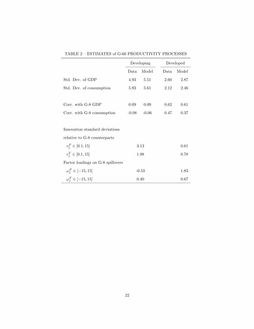
TABLE 2 – ESTIMATES of G-60 PRODUCTIVITY PROCESSES

Developing Developed

Data Model Data Model

Std. Dev. of GDP 4.93 5.51 2.60 2.87

Std. Dev. of consumption 5.93 5.61 2.12 2.46

Corr. with G-8 GDP 0.09 0.09 0.62 0.61

Corr. with G-8 consumption -0.08 -0.06 0.47 0.37

Innovation standard deviations

relative to G-8 counterparts

vPj ∈ [0.1, 15] 3.13 0.61

vTj ∈ [0.1, 15] 1.98 0.78

Factor loadings on G-8 spillovers

ωPj ∈ [−15, 15] -0.53 1.83

ωTj ∈ [−15, 15] 0.40 0.67

22

TABLE 3 – BOND PRICE SHOCK PARAMETERS

Developing Developed

Spillovers Yes No Yes No

Persistence 0.30 0.54 0.24 0.69

Innovation standard deviations 0.003 0.006 0.004 0.005

23

TABLE 4. OUTPUT VARIANCE DECOMPOSITIONS, SMALL OPEN ECONOMY MODEL

Variance Decomposition Number Std. dev.

Source of shock Home Home World Total of of

Type of shock Permanent Transitory Interest rate Countries Output

All Countries 36.93 36.97 26.10 100 58 4.3

Developing 43.13 30.51 26.37 100 40 4.9

Developed 23.15 51.34 25.51 100 18 2.8

AG Sample 25.70 46.72 27.58 100 20 3.1

Developing 29.97 43.03 27.00 100 9 4.0

Developed 21.81 50.07 18.12 100 11 2.3

Notes:Productivity spillovers are abstracted from in this specification because they would

not be identified using the small open economy model.

24

TABLE 5. OUTPUT VARIANCE DECOMPOSITIONS, MODEL COMPARISONS

Model DSGE SOE

Source of shock Home + G8 Home + G8 Home + G8 Home + G8 Interest

Type of shock Permanent Transitory Permanent Transitory rate

All Countries 46.9 53.1 41.3 53.2 5.4

Developing 45.2 54.8 42.8 54.4 2.7

Developed 50.8 49.2 38.0 50.5 11.5

Aguiar and Gopinath 43.3 56.7 32.6 57.0 10.4

Developing 34.9 65.1 30.2 64.0 5.8

Developed 51.0 49.0 34.8 50.8 14.4

Source of shock Home G8 Home G8 Home G8 Home G8 Interest

Type of shock P P T T P P T T rate

All Countries 23.6 23.4 38.5 14.6 22.5 18.8 37.9 15.3 5.4

Developing 30.6 14.6 44.2 10.6 29.5 13.4 43.6 10.8 2.7

Developed 8.1 42.7 25.8 23.4 7.1 30.9 25.3 25.2 11.5

25

26

Figure 1. International Business Cycles

0

0.05

0.1

0.15

Output std. dev. Consumption std. dev.

27

Figure 2. Proportion of output growth variance accounted for by permanent shocks:

Comparison of DSGE model and SOE with productivity spillovers

0

10

20

30

40

50

60

70

80

90

100

DSGE permanent component SOE permanent component with spillovers

28

Figure 3. Proportion of output growth variance accounted by permanent shocks:

Comparison of SOE model with productivity spillovers to SOE model without spillovers

0

10

20

30

40

50

60

70

80

90

100

SOE permanent component (with spillovers) SOE permanent component (w/o spillovers)