Working Paper No. 577

Explaining the Gender Wage Gap in Georgia

by

Tamar Khitarishvili*Bard College

September 2009

*The author thanks the Georgian Statistics Department for providing the data and theNational Council for European and Eurasian Research for financial support. She isespecially grateful to Rania Antonopoulos for her encouragement in pursuing the analysisof the gender wage gap in Georgia and throughout her work on this paper. Commentsmay be sent to khitaris@bard.edu.

The Levy Economics Institute Working Paper Collection presents research in progress byLevy Institute scholars and conference participants. The purpose of the series is todisseminate ideas to and elicit comments from academics and professionals.

The Levy Economics Institute of Bard College, founded in 1986, is a nonprofit,nonpartisan, independently funded research organization devoted to public service.Through scholarship and economic research it generates viable, effective public policyresponses to important economic problems that profoundly affect the quality of life inthe United States and abroad.

The Levy Economics InstituteP.O. Box 5000

Annandale-on-Hudson, NY 12504-5000http://www.levy.org

Copyright © The Levy Economics Institute 2009 All rights reserved.

1

ABSTRACT

This paper evaluates gender wage differentials in Georgia between 2000 and 2004. Using

ordinary least squares, we find that the gender wage gap in Georgia is substantially

higher than in other transition countries. Correcting for sample selection bias using the

Heckman approach further increases the gender wage gap. The Blinder Oaxaca

decomposition results suggest that most of the wage gap remains unexplained. The

explained portion of the gap is almost entirely attributed to industrial variables. We find

that the gender wage gap in Georgia diminished between 2000 and 2004.

Keywords: Gender Wage Gap; Economic Transition; Georgia

JEL Classifications: J16, J31, P20

2

The breakdown of the Soviet Union has led to a dramatic economic and social

transformation of the Socialist-bloc countries. Increased income inequality has been an

unwelcome feature of this transformation in many of these countries. A growing body of

literature focuses on the gender dimension of income inequality in this region, where

gender equality was lauded as one of the greatest achievements of its former economic

system.

This paper contributes to the literature by evaluating the case of Georgia. The

paper focuses on a particular aspect of gender inequality, namely the gender wage gap.

The objective of the paper is to evaluate gender wage differentials in Georgia during

2000–2004 and to explain their sources. We assess this issue by estimating a Mincerian

wage earnings equation with education, experience, and other relevant characteristics as

dependent variables and evaluate whether, controlling for these factors, women are

remunerated differently from men. We adjust the results for sample selection bias and

implement the Blinder-Oaxaca decomposition of the male-female wage gap to identify its

causes.

BACKGROUND

Evidence from the Soviet period indicates that the gender wage gap in the Soviet Union

was comparable to Western countries (Ofer and Vinokur 1992). The breakdown of the

Soviet Union eliminated institutional mechanisms aimed at maintaining gender wage

equality and in many countries resulted in the widening of the gap. Although systematic

assessment of the situation in Georgia is lacking, available evidence indicates that this is

in fact what happened in early 1990s (Yemtsov 2001).

Zooming forward to the most recent past, the Georgian government has taken

specific steps aimed at advancing the cause of gender equality. Among most recent

changes, in 2004, the Gender Equality Advisory Council was established under the

Parliament Speaker’s office. In 2005, the Government Commission on Gender Equality

(GCGE) was created with a one-year mandate of drafting the National Action Plan for

strengthening gender equality. The goal of the Action Plan was to “facilitate the

development and adoption of relevant monitoring mechanisms to plan and review

3

implementation of government obligations to gender equality” (Jashi 2005). In February

2006, the commission and the council set up a joint working group, which produced the

Gender Equality Strategy of Georgia (Sabedashvili 2007: 25). This document was

presented as “The State Concept on Gender Equality” before the Parliament of Georgia

and approved by it in July 2006. However, it has not yet translated into any plan of action

for internalizing the gender framework into political, social, and economic decision-

making. As a member of the Committee on Elimination of Discrimination against

Women pointed out during the meeting with the Georgian representatives, “in practice,

many of women’s rights [in Georgia are] violated, for example in the field of

employment. It [is] not enough to introduce legislation for gender equality—it [is] also

important to ensure equality in practice” (CEDAW 2006).

It appears that in the Georgian society gender equality as a societal goal is

perceived as a concept imposed from outside and potentially threatening the traditional

way of life. Sabedashvili (2007: 24–25) points out that in practice gender equality efforts

in Georgia are supported almost exclusively by international donor organizations, which

contributes to this perception. It is noteworthy that, according to one survey, 45.4% of the

respondents indicate that in their view men and women in Georgia are, in fact, equal

(Sumbadze 2008).1

Yet, the evidence on political representation points to the contrary. As of 2006,

there were no female city mayors in Georgia (Sumbadze 2008). In 2008, only 7 out of

139 members of Parliament were women (5%) (Department of Statitics 2008). As of

January 2009, there were no women in the ministerial level positions of the Georgian

government.

The focus of this study is on assessing the economic dimension of gender

inequality in Georgia, covering the late transition period from 2000 until 2004, when

institutional shifts described above started taking place. Therefore, this study aims at

establishing a baseline for the future analysis of the impact of gender targeted policies.

Previous work empirically evaluating the gender wage gap in Georgia is very

limited. Jashi (2005) provides an excellent descriptive assessment of the gender issues

currently facing Georgia. Her survey summarizes recent demographic and socioeconomic

1 The survey was conducted in 2007 by the Institute of Policy Studies.

4

trends observed among men and women. Yemtsov (2001) evaluates the connection

between the labor market conditions and poverty in Georgia using 1992–1995 household

survey data. He briefly mentions the presence of substantial differences in pay between

men and women in Georgia during 1992–1995. However, he does not explicitly quantify

these differences; nor does he attempt to explain their presence.

At the same time, the gender wage gap literature on transition countries is

expanding and can be used to place Georgia in the context of other countries in the

region. A number of studies analyze the Russian case. Among them are Brainerd (1998),

Newell and Reilly (1996), Reilly (1999), Arabsheibani and Lau (1999), Glinskaya and

Mroz (2000), Gerry et al. (2004), Cheidvasser and Benitez Silva (2007), Kazakova

(2007), and Johnes and Tanaka (2008). According to these studies, in Russia the

female/male wage ratio varies from 0.60 (reported for 1994 in Brainerd [1998]) to 0.78

(reported for 1995 in Glinskaya and Mroz [2000]). Brainerd (2000) analyzes a number of

Central and Eastern European countries, among which are three former Soviet Union

countries: Russia, Ukraine, and Estonia. She finds that in 1994, in Russia, women earned

68% of what men did. These numbers in Ukraine and Estonia were 60% and 74%,

respectively. Anderson and Pomfret (2003) analyze the Kyrgyz data and find that the

female-male wage ratio was 66% in 1993 and it increased to 83% in 1997. However,

more recent evidence points to the worsening of the situation. According to the Asian

Development Bank’s Gender Assessment Report (ADB 2005), as of 2000, Kyrgyz

women earned 67.6% of what men did and by 2002 the ratio declined further to 64.9%.

Most studies find that individual characteristics explain a very small portion of the gender

wage differentials. In fact, Anderson and Pomfret (2003) conclude that in Kyrgyzstan in

1993 and 1997, controlling for individual characteristics, women’s wages should have

been higher than men’s wages.

DATA OVERVIEW

The 2000–2004 dataset in this study comes from the Georgian Household Budget Survey

(HBS) run by the Georgian Department of Statistics. It is based on a quarterly survey of

3,351 households.

5

This analysis is focused on investigating gender wage differentials among

individuals who work for pay.2 The sample in the analysis is restricted to the men

between 16–64 years old and women 16–59 years old. Employed individuals earning

zero income are excluded from the sample.3

Wages are defined in terms of monthly wage income from main employment,

expressed in Georgian laris. For comparison purposes, we normalize all wage data in

terms of year 2000 using official CPI data (Georgian Statistical Yearbook 2006). The

education variable is years of education imputed from the data. Following the literature,

experience is constructed as age minus schooling minus 6. Regional and industrial

variables are dummy variables, which take the value of 1 when the respondent lives in the

corresponding region or works in a corresponding industry. Tbilisi is the reference

region. Agriculture is the reference sector. The urban variable takes the value of 1 for

urban regions and 0 otherwise.

Based on the dataset, Georgian women are more educated than Georgian men.

Their mean years of education are 11.9 as opposed to 11.85 for men, although the

difference is not statistically significant.

In interpreting the labor force data from the household survey, the peculiarities of

the household questionnaire need to be taken into consideration. The reported

employment categories are nonworking age, hired employed, self-employed, or not-

employed (individuals who have no job, regardless of whether they are searching for one

or not4). The nonworking age category includes individuals younger than 16 years of age.

The not-employed category lumps together nonworking individuals looking for a job

(officially unemployed individuals) and those who, for a number of reasons (e.g.,

retirement or taking care of children), are not looking for a job. As a result, both the labor

force participation rate and the unemployment rate calculated from the household survey

are likely to be overestimated. Moreover, assuming that a greater proportion of women

than men in Georgia are out of the labor force, the participation rate of women is likely to

2 A number of studies focus on assessing gender wage inequality among self-employed (Hundley 2000; Eastough and Miller 2004). 3 The employed zero-earning group constitutes 1.8% of the sample. 4 As opposed to unemployed defined to be individuals without work, available for work, and looking for work, see http://laborsta.ilo.org/applv8/data/c3e.html.

6

be overestimated more than it is for men. The same can be said about the unemployment

rate.

In addition, in the case of the labor force participation rate, the different

retirement ages of women and men influence the estimates. Recall that women between

the age of 16 and 59 are included in the sample, whereas for men the age range is

between 16 and 64.

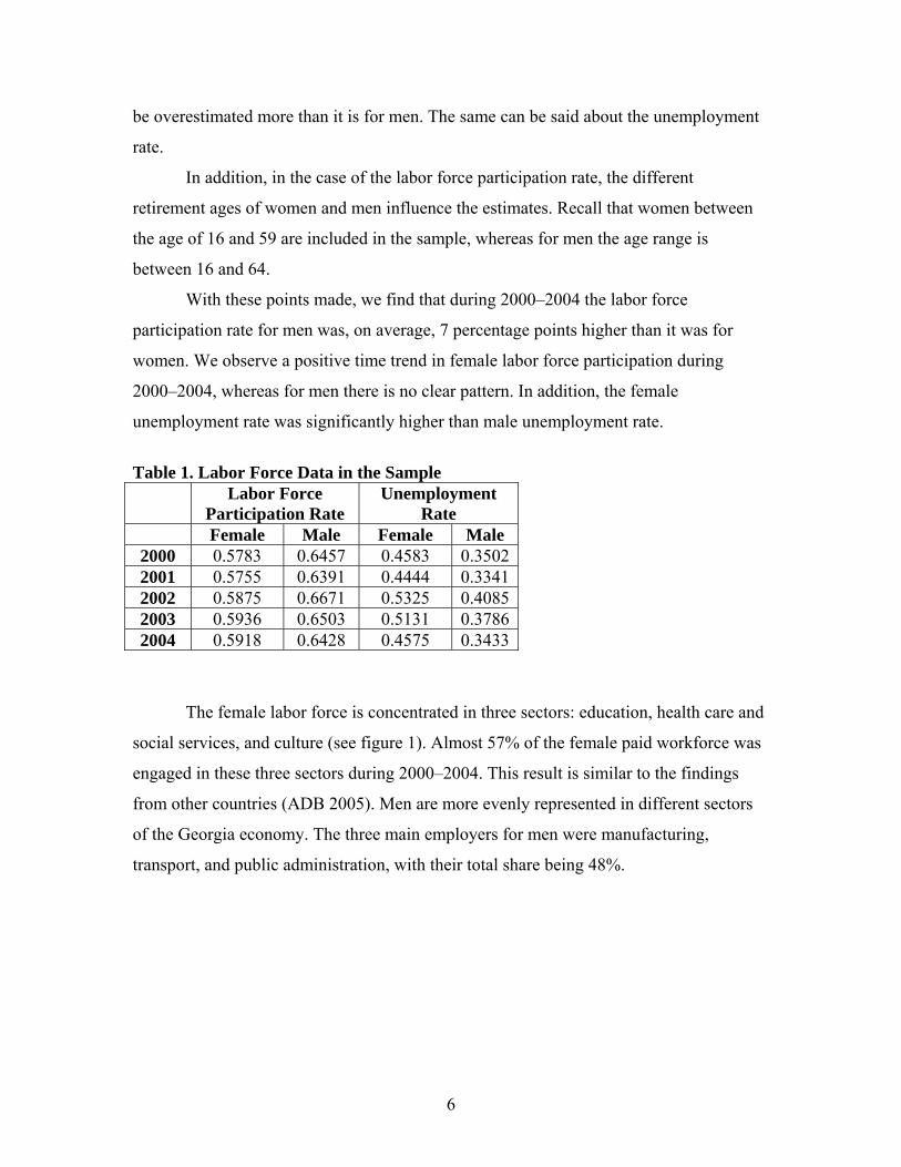
With these points made, we find that during 2000–2004 the labor force

participation rate for men was, on average, 7 percentage points higher than it was for

women. We observe a positive time trend in female labor force participation during

2000–2004, whereas for men there is no clear pattern. In addition, the female

unemployment rate was significantly higher than male unemployment rate.

Table 1. Labor Force Data in the Sample

Labor Force Participation Rate

Unemployment Rate

Female Male Female Male 2000 0.5783 0.6457 0.4583 0.35022001 0.5755 0.6391 0.4444 0.33412002 0.5875 0.6671 0.5325 0.40852003 0.5936 0.6503 0.5131 0.37862004 0.5918 0.6428 0.4575 0.3433

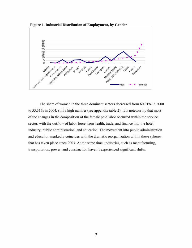
The female labor force is concentrated in three sectors: education, health care and

social services, and culture (see figure 1). Almost 57% of the female paid workforce was

engaged in these three sectors during 2000–2004. This result is similar to the findings

from other countries (ADB 2005). Men are more evenly represented in different sectors

of the Georgia economy. The three main employers for men were manufacturing,

transport, and public administration, with their total share being 48%.

7

Figure 1. Industrial Distribution of Employment, by Gender

05

10152025303540

Mining

Intern

ation

al org

aniza

tions

Constr

uction

Hired h

ouse

hold la

bor

Agricu

lture

Power

Finance

Hotels

Real E

state

Transpo

rt

Culture

Manufac

turing

Public

admini

strati

onTrade

Health

Educa

tion

Men Women

The share of women in the three dominant sectors decreased from 60.91% in 2000

to 55.31% in 2004, still a high number (see appendix table 2). It is noteworthy that most

of the changes in the composition of the female paid labor occurred within the service

sector, with the outflow of labor force from health, trade, and finance into the hotel

industry, public administration, and education. The movement into public administration

and education markedly coincides with the dramatic reorganization within these spheres

that has taken place since 2003. At the same time, industries, such as manufacturing,

transportation, power, and construction haven’t experienced significant shifts.

8

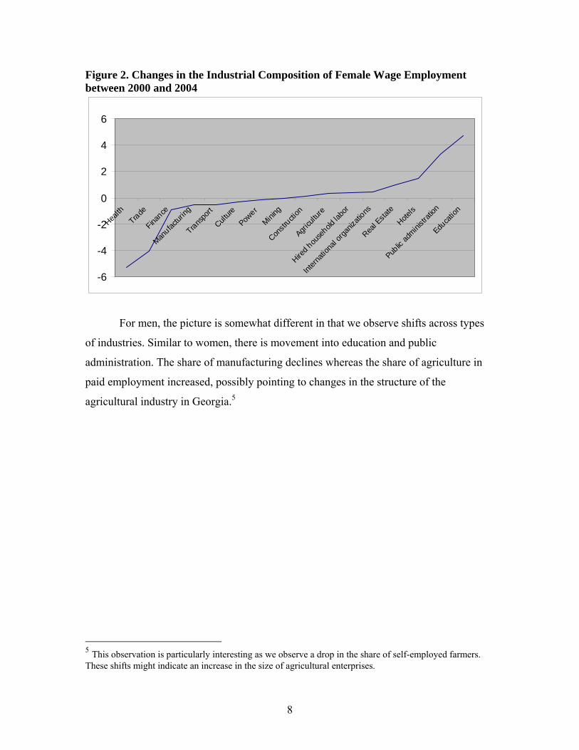
Figure 2. Changes in the Industrial Composition of Female Wage Employment between 2000 and 2004

-6

-4

-2

0

2

4

6

Health

Trade

Finance

Manufac

turing

Transpo

rt

Culture

Power

Mining

Constr

uction

Agricu

lture

Hired h

ouse

hold la

bor

Intern

ation

al org

aniza

tions

Real E

state

Hotels

Public

admini

strati

on

Educa

tion

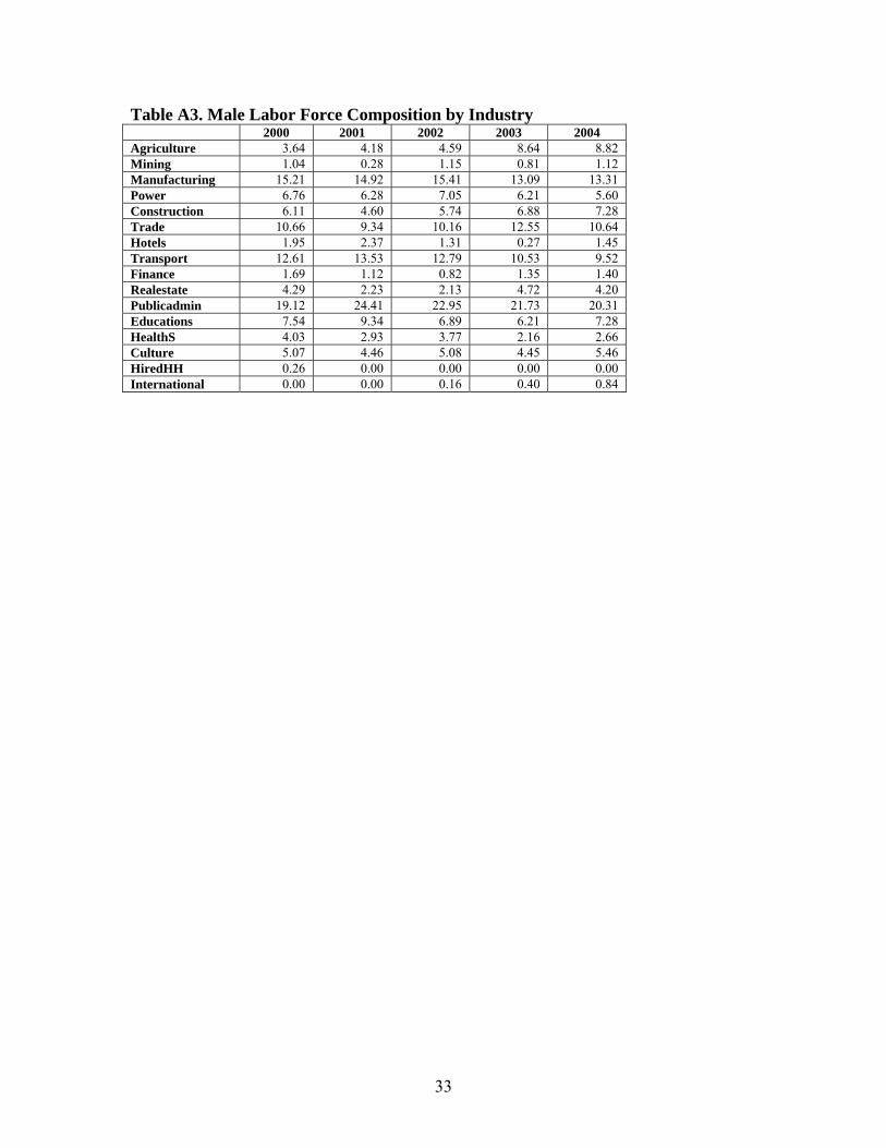
For men, the picture is somewhat different in that we observe shifts across types

of industries. Similar to women, there is movement into education and public

administration. The share of manufacturing declines whereas the share of agriculture in

paid employment increased, possibly pointing to changes in the structure of the

agricultural industry in Georgia.5

5 This observation is particularly interesting as we observe a drop in the share of self-employed farmers. These shifts might indicate an increase in the size of agricultural enterprises.

9

Figure 3. Changes in the Industrial Composition of Male Wage Employment, 2000–2004

-6

-4

-2

0

2

4

6

Transp

ort

Manufa

cturin

gTrad

ePow

er

Health

Financ

eHote

ls

Intern

ation

al org

aniza

tions

Real E

state

Mining

Culture

Hired h

ouse

hold

labor

Constr

uctio

n

Educa

tion

Public

admini

strati

on

Agricu

lture

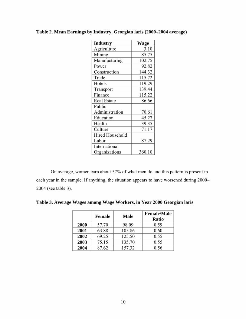
High occupational concentration observed among Georgian women is not

uncommon. Some degree of occupational segregation is observed in most countries

(Dolado, Felgueroso, and Jimeno 2002). However, because “female” occupations tend to

pay less, women, on average, receive lower earnings than men based on the occupational

characteristics. In fact, agriculture together with education, health care, and culture—the

industries with the highest concentration of women—are the lowest paying industries in

the Georgian economy (see table 2).

10

Table 2. Mean Earnings by Industry, Georgian laris (2000–2004 average)

Industry Wage Agriculture 3.10 Mining 85.75 Manufacturing 102.75 Power 92.82 Construction 144.32 Trade 115.72 Hotels 119.29 Transport 139.44 Finance 115.22 Real Estate 86.66 Public Administration 70.61 Education 45.27 Health 39.35 Culture 71.17 Hired Household Labor 87.29 International Organizations 360.10

On average, women earn about 57% of what men do and this pattern is present in

each year in the sample. If anything, the situation appears to have worsened during 2000–

2004 (see table 3).

Table 3. Average Wages among Wage Workers, in Year 2000 Georgian laris

Female Male Female/Male Ratio

2000 57.70 98.09 0.59 2001 63.88 105.86 0.60 2002 69.25 125.50 0.55 2003 75.15 135.70 0.55 2004 87.62 157.32 0.56

11

METHODOLOGY

There are large variations in the approaches and variables used for estimating the gender

wage gap (Weichselbaumer and Winter-Ebmer 2005). The choice of approach affects the

size of the estimated gender wage gap, as well as the estimates of the gender wage

discrimination. So does the choice of variables and the inclusion of different groups of

individuals.

To enable the comparison of the Georgian case to the studies of other countries,

we use an augmented version of the conventional Mincerian earnings equation (Mincer

1974):

lnwj = α+Xjβ +εj, (1)

where subscript j denotes individual j, variable wj stands for monthly wages of individual

j, Xj is a vector of explanatory variables for individual j, which includes schooling,

experience, experience squared, gender, and geographic and industry-level

characteristics.6

The Mincerian earnings equation is first estimated using an ordinary least squares

(OLS) approach. The potential presence of a correlation between the matrix of regressors

and the error term has been shown to lead to inconsistent (and biased, in the small sample

case) coefficient estimates (Card 1999 and 2001). In the case of the Mincerian earnings

equation, there are several potential sources of correlation between the regressors and the

error term. Khitarishvili (2008) uses the instrumental variables approach to test for the

presence of endogeneity in the education variable and does not find sufficient evidence to

reject the hypothesis of exogeneity of education.

In this study we test and correct for another potential source of correlation:

sample selection bias. If the selection of individuals into the category of wage earners is

not random, the coefficient estimates in the wage equation can be biased. We use the

Heckman sample-selection correction method (Heckman 1979) to test and correct for the 6 The use of industrial dummies in the wage equation in the context of gender wage decomposition has been discussed in Blau and Ferber (1987). They suggest that including industrial dummies provides a lower bound on the discrimination whereas excluding them provides an upper bound.

12

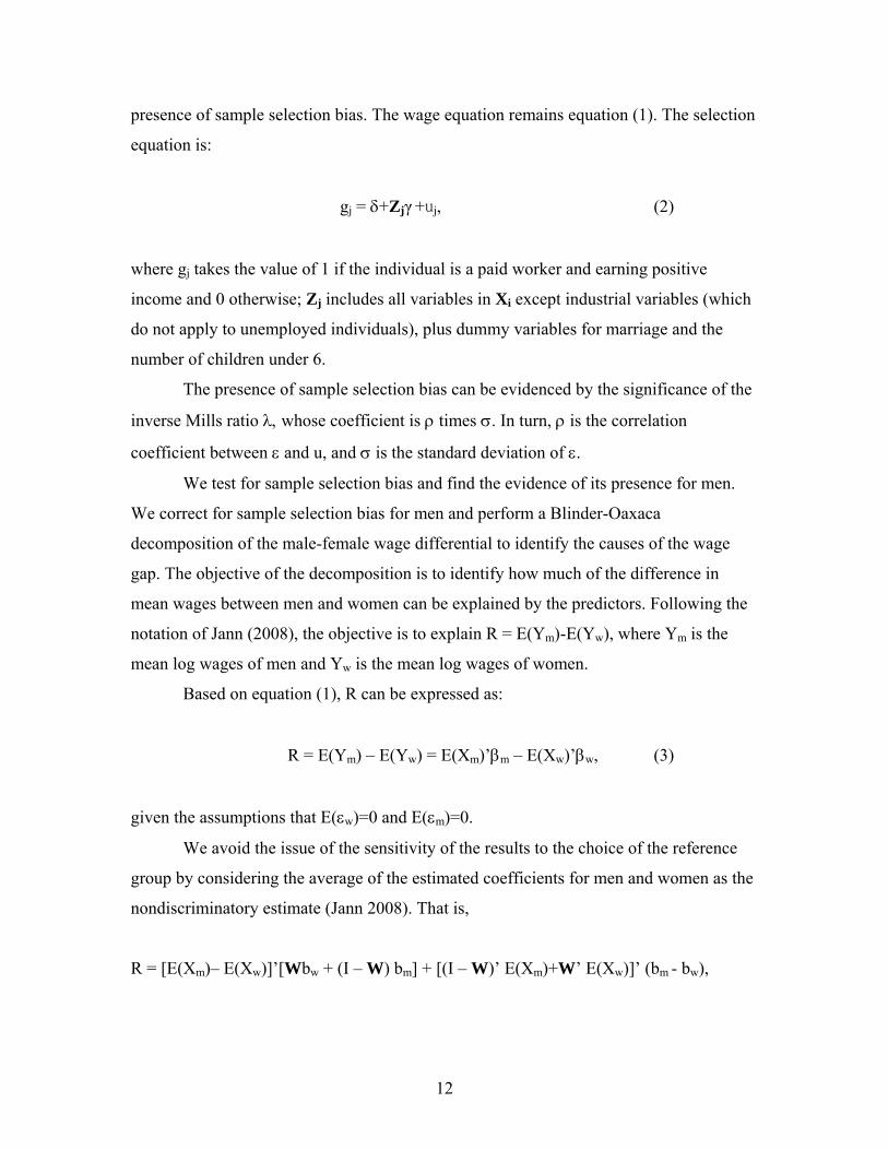
presence of sample selection bias. The wage equation remains equation (1). The selection

equation is:

gj = δ+Zjγ +uj, (2)

where gj takes the value of 1 if the individual is a paid worker and earning positive

income and 0 otherwise; Zj includes all variables in Xi except industrial variables (which

do not apply to unemployed individuals), plus dummy variables for marriage and the

number of children under 6.

The presence of sample selection bias can be evidenced by the significance of the

inverse Mills ratio λ, whose coefficient is ρ times σ. In turn, ρ is the correlation

coefficient between ε and u, and σ is the standard deviation of ε.

We test for sample selection bias and find the evidence of its presence for men.

We correct for sample selection bias for men and perform a Blinder-Oaxaca

decomposition of the male-female wage differential to identify the causes of the wage

gap. The objective of the decomposition is to identify how much of the difference in

mean wages between men and women can be explained by the predictors. Following the

notation of Jann (2008), the objective is to explain R = E(Ym)-E(Yw), where Ym is the

mean log wages of men and Yw is the mean log wages of women.

Based on equation (1), R can be expressed as:

R = E(Ym) – E(Yw) = E(Xm)’βm – E(Xw)’βw, (3)

given the assumptions that E(εw)=0 and E(εm)=0.

We avoid the issue of the sensitivity of the results to the choice of the reference

group by considering the average of the estimated coefficients for men and women as the

nondiscriminatory estimate (Jann 2008). That is,

R = [E(Xm)– E(Xw)]’[Wbw + (I – W) bm] + [(I – W)’ E(Xm)+W’ E(Xw)]’ (bm - bw),

13

where W = 0.5I. The first component of R is explained by the predictor differences

between men and women and the second component is the unexplained part.

A substantial unexplained component is commonly attributed to gender

discrimination, although it might reflect the omission of important variables (Jann 2008).

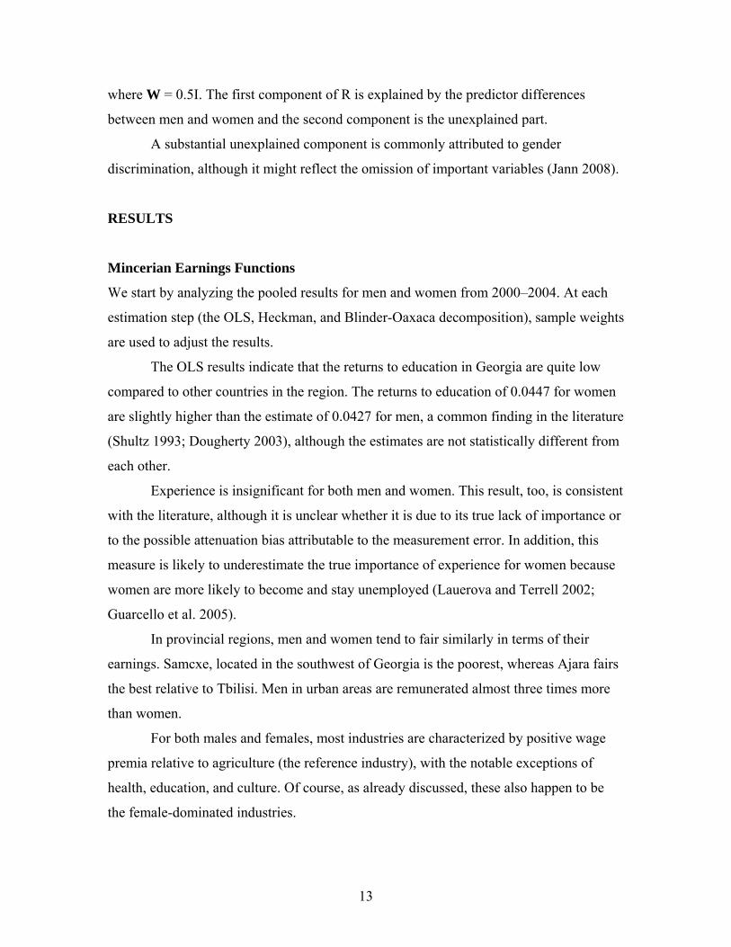
RESULTS

Mincerian Earnings Functions

We start by analyzing the pooled results for men and women from 2000–2004. At each

estimation step (the OLS, Heckman, and Blinder-Oaxaca decomposition), sample weights

are used to adjust the results.

The OLS results indicate that the returns to education in Georgia are quite low

compared to other countries in the region. The returns to education of 0.0447 for women

are slightly higher than the estimate of 0.0427 for men, a common finding in the literature

(Shultz 1993; Dougherty 2003), although the estimates are not statistically different from

each other.

Experience is insignificant for both men and women. This result, too, is consistent

with the literature, although it is unclear whether it is due to its true lack of importance or

to the possible attenuation bias attributable to the measurement error. In addition, this

measure is likely to underestimate the true importance of experience for women because

women are more likely to become and stay unemployed (Lauerova and Terrell 2002;

Guarcello et al. 2005).

In provincial regions, men and women tend to fair similarly in terms of their

earnings. Samcxe, located in the southwest of Georgia is the poorest, whereas Ajara fairs

the best relative to Tbilisi. Men in urban areas are remunerated almost three times more

than women.

For both males and females, most industries are characterized by positive wage

premia relative to agriculture (the reference industry), with the notable exceptions of

health, education, and culture. Of course, as already discussed, these also happen to be

the female-dominated industries.

14

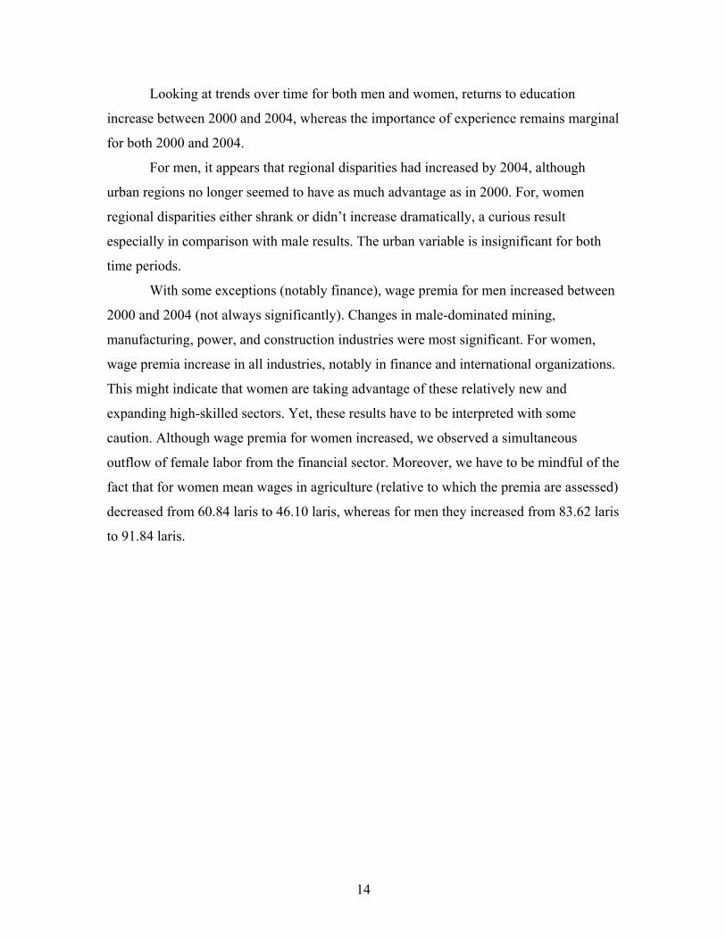
Looking at trends over time for both men and women, returns to education

increase between 2000 and 2004, whereas the importance of experience remains marginal

for both 2000 and 2004.

For men, it appears that regional disparities had increased by 2004, although

urban regions no longer seemed to have as much advantage as in 2000. For, women

regional disparities either shrank or didn’t increase dramatically, a curious result

especially in comparison with male results. The urban variable is insignificant for both

time periods.

With some exceptions (notably finance), wage premia for men increased between

2000 and 2004 (not always significantly). Changes in male-dominated mining,

manufacturing, power, and construction industries were most significant. For women,

wage premia increase in all industries, notably in finance and international organizations.

This might indicate that women are taking advantage of these relatively new and

expanding high-skilled sectors. Yet, these results have to be interpreted with some

caution. Although wage premia for women increased, we observed a simultaneous

outflow of female labor from the financial sector. Moreover, we have to be mindful of the

fact that for women mean wages in agriculture (relative to which the premia are assessed)

decreased from 60.84 laris to 46.10 laris, whereas for men they increased from 83.62 laris

to 91.84 laris.

15

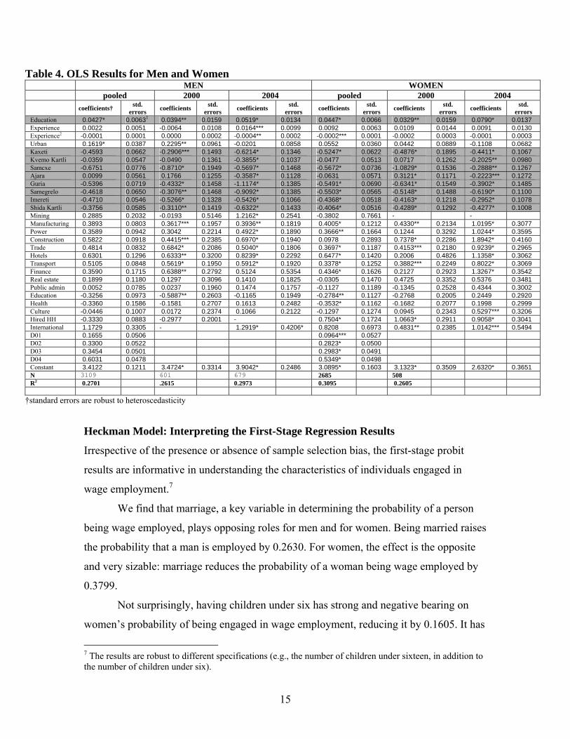
Table 4. OLS Results for Men and Women MEN WOMEN pooled 2000 2004 pooled 2000 2004 coefficients† std.

errors coefficients std. errors coefficients std.

errors coefficients std. errors coefficients std.

errors coefficients std. errors

Education 0.0427* 0.00631 0.0394** 0.0159 0.0519* 0.0134 0.0447* 0.0066 0.0329** 0.0159 0.0790* 0.0137 Experience 0.0022 0.0051 -0.0064 0.0108 0.0164*** 0.0099 0.0092 0.0063 0.0109 0.0144 0.0091 0.0130 Experience2 -0.0001 0.0001 0.0000 0.0002 -0.0004** 0.0002 -0.0002*** 0.0001 -0.0002 0.0003 -0.0001 0.0003 Urban 0.1619* 0.0387 0.2295** 0.0961 -0.0201 0.0858 0.0552 0.0360 0.0442 0.0889 -0.1108 0.0682 Kaxeti -0.4593 0.0662 -0.2906*** 0.1493 -0.6214* 0.1346 -0.5247* 0.0622 -0.4876* 0.1895 -0.4411* 0.1067 Kvemo Kartli -0.0359 0.0547 -0.0490 0.1361 -0.3855* 0.1037 -0.0477 0.0513 0.0717 0.1262 -0.2025** 0.0980 Samcxe -0.6751 0.0776 -0.8710* 0.1949 -0.5697* 0.1468 -0.5672* 0.0736 -1.0829* 0.1536 -0.2888** 0.1267 Ajara 0.0099 0.0561 0.1766 0.1255 -0.3587* 0.1128 -0.0631 0.0571 0.3121* 0.1171 -0.2223*** 0.1272 Guria -0.5396 0.0719 -0.4332* 0.1458 -1.1174* 0.1385 -0.5491* 0.0690 -0.6341* 0.1549 -0.3902* 0.1485 Samegrelo -0.4618 0.0650 -0.3076** 0.1468 -0.9092* 0.1385 -0.5503* 0.0565 -0.5148* 0.1488 -0.6190* 0.1100 Imereti -0.4710 0.0546 -0.5266* 0.1328 -0.5426* 0.1066 -0.4368* 0.0518 -0.4163* 0.1218 -0.2952* 0.1078 Shida Kartli -0.3756 0.0585 -0.3110** 0.1419 -0.6322* 0.1433 -0.4064* 0.0516 -0.4289* 0.1292 -0.4277* 0.1008 Mining 0.2885 0.2032 -0.0193 0.5146 1.2162* 0.2541 -0.3802 0.7661 - - Manufacturing 0.3893 0.0803 0.3617*** 0.1957 0.3936** 0.1819 0.4005* 0.1212 0.4330** 0.2134 1.0195* 0.3077 Power 0.3589 0.0942 0.3042 0.2214 0.4922* 0.1890 0.3666** 0.1664 0.1244 0.3292 1.0244* 0.3595 Construction 0.5822 0.0918 0.4415*** 0.2385 0.6970* 0.1940 0.0978 0.2893 0.7378* 0.2286 1.8942* 0.4160 Trade 0.4814 0.0832 0.6842* 0.2086 0.5040* 0.1806 0.3697* 0.1187 0.4153*** 0.2180 0.9239* 0.2965 Hotels 0.6301 0.1296 0.6333** 0.3200 0.8239* 0.2292 0.6477* 0.1420 0.2006 0.4826 1.1358* 0.3062 Transport 0.5105 0.0848 0.5619* 0.1950 0.5912* 0.1920 0.3378* 0.1252 0.3882*** 0.2249 0.8022* 0.3069 Finance 0.3590 0.1715 0.6388** 0.2792 0.5124 0.5354 0.4346* 0.1626 0.2127 0.2923 1.3267* 0.3542 Real estate 0.1899 0.1180 0.1297 0.3096 0.1410 0.1825 -0.0305 0.1470 0.4725 0.3352 0.5376 0.3481 Public admin 0.0052 0.0785 0.0237 0.1960 0.1474 0.1757 -0.1127 0.1189 -0.1345 0.2528 0.4344 0.3002 Education -0.3256 0.0973 -0.5887** 0.2603 -0.1165 0.1949 -0.2784** 0.1127 -0.2768 0.2005 0.2449 0.2920 Health -0.3360 0.1586 -0.1581 0.2707 0.1613 0.2482 -0.3532* 0.1162 -0.1682 0.2077 0.1998 0.2999 Culture -0.0446 0.1007 0.0172 0.2374 0.1066 0.2122 -0.1297 0.1274 0.0945 0.2343 0.5297*** 0.3206 Hired HH -0.3330 0.0883 -0.2977 0.2001 - 0.7504* 0.1724 1.0663* 0.2911 0.9058* 0.3041 International 1.1729 0.3305 - 1.2919* 0.4206* 0.8208 0.6973 0.4831** 0.2385 1.0142*** 0.5494 D01 0.1655 0.0506 0.0964*** 0.0527 D02 0.3300 0.0522 0.2823* 0.0500 D03 0.3454 0.0501 0.2983* 0.0491 D04 0.6031 0.0478 0.5349* 0.0498 Constant 3.4122 0.1211 3.4724* 0.3314 3.9042* 0.2486 3.0895* 0.1603 3.1323* 0.3509 2.6320* 0.3651 N 3109 601 679 2685 508 R2 0.2701 .2615 0.2973 0.3095 0.2605

†standard errors are robust to heteroscedasticity

Heckman Model: Interpreting the First-Stage Regression Results

Irrespective of the presence or absence of sample selection bias, the first-stage probit

results are informative in understanding the characteristics of individuals engaged in

wage employment.7

We find that marriage, a key variable in determining the probability of a person

being wage employed, plays opposing roles for men and for women. Being married raises

the probability that a man is employed by 0.2630. For women, the effect is the opposite

and very sizable: marriage reduces the probability of a woman being wage employed by

0.3799.

Not surprisingly, having children under six has strong and negative bearing on

women’s probability of being engaged in wage employment, reducing it by 0.1605. It has

7 The results are robust to different specifications (e.g., the number of children under sixteen, in addition to the number of children under six).

16

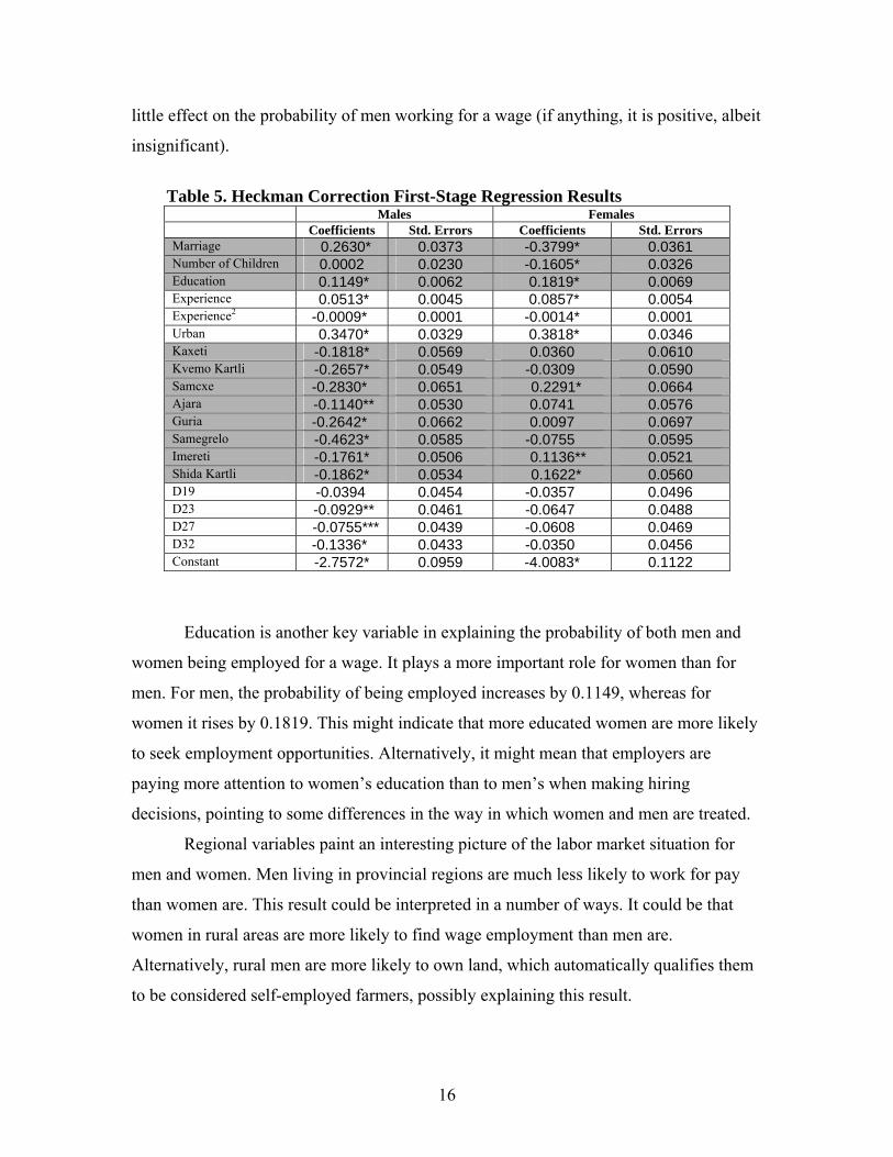
little effect on the probability of men working for a wage (if anything, it is positive, albeit

insignificant).

Table 5. Heckman Correction First-Stage Regression Results

Males Females Coefficients Std. Errors Coefficients Std. Errors

Marriage 0.2630* 0.0373 -0.3799* 0.0361 Number of Children 0.0002 0.0230 -0.1605* 0.0326 Education 0.1149* 0.0062 0.1819* 0.0069 Experience 0.0513* 0.0045 0.0857* 0.0054 Experience2 -0.0009* 0.0001 -0.0014* 0.0001 Urban 0.3470* 0.0329 0.3818* 0.0346 Kaxeti -0.1818* 0.0569 0.0360 0.0610 Kvemo Kartli -0.2657* 0.0549 -0.0309 0.0590 Samcxe -0.2830* 0.0651 0.2291* 0.0664 Ajara -0.1140** 0.0530 0.0741 0.0576 Guria -0.2642* 0.0662 0.0097 0.0697 Samegrelo -0.4623* 0.0585 -0.0755 0.0595 Imereti -0.1761* 0.0506 0.1136** 0.0521 Shida Kartli -0.1862* 0.0534 0.1622* 0.0560 D19 -0.0394 0.0454 -0.0357 0.0496 D23 -0.0929** 0.0461 -0.0647 0.0488 D27 -0.0755*** 0.0439 -0.0608 0.0469 D32 -0.1336* 0.0433 -0.0350 0.0456 Constant -2.7572* 0.0959 -4.0083* 0.1122

Education is another key variable in explaining the probability of both men and

women being employed for a wage. It plays a more important role for women than for

men. For men, the probability of being employed increases by 0.1149, whereas for

women it rises by 0.1819. This might indicate that more educated women are more likely

to seek employment opportunities. Alternatively, it might mean that employers are

paying more attention to women’s education than to men’s when making hiring

decisions, pointing to some differences in the way in which women and men are treated.

Regional variables paint an interesting picture of the labor market situation for

men and women. Men living in provincial regions are much less likely to work for pay

than women are. This result could be interpreted in a number of ways. It could be that

women in rural areas are more likely to find wage employment than men are.

Alternatively, rural men are more likely to own land, which automatically qualifies them

to be considered self-employed farmers, possibly explaining this result.

17

Heckman Model: Evidence of Sample Selection Bias

The selection equation in the Heckman model includes marriage and the number of

children under six years old as identifying variables. We do not use industrial variables,

as they do not apply to the unemployed.

The coefficient on λ is significant for men, indicating the presence of sample

selection bias, whereas for women it is insignificant. This result is important as it

indicates the presence of different mechanisms describing the selection into wage work

for men and women. A number of studies conducted on transition countries find no

evidence of sample selection bias (Gerry et al. 2004), while others conduct sample

selection bias correction only for women, implicitly assuming that sample selection bias

is an issue only for the female population (Arabsheibani and Lau 1999; Arabsheibani and

Mussurov 2007). The results in this study point to a need to pay more attention to the

causes of sample selection bias among men as well as women.

A key finding, which has received little to no attention in the literature, is the sign

of the λ coefficient, σρ, which is negative for both men and women. Given that σ is

positive, the key factor determining the sign of the coefficient is ρ. The significance of

the coefficient of λ points to the mere presence of sample selection bias, however its sign

has direct bearing on the results of the Blinder-Oaxaca decomposition as, under negative

ρ, mean wages are underestimated. Thus, finding a negative and significant coefficient

for men implies the need for correction only for men, which results in an increase in

men’s mean wages without a corresponding increase in the mean wages for women.

Thus, the gender wage gap with correction for sample selection bias will be higher than

without it (a result corroborated by findings in the literature although, again, not

sufficiently analyzed).

The negative ρ indicates that characteristics that raise an individual’s salary in

fact reduce this person’s probability of being employed. Given that the coefficient on λ is

significant and its value is higher for men than it is for women, we can infer that for men,

much more so than for women, factors that lead to their earning higher wages are also

factors responsible for their not being hired.

There has been a rise in the number of studies that obtain negative estimates of

ρ (see Dolton and Makepeace [1986] for an early work). Given the counterintuitive

18

nature of this result, the vast majority of studies either does not address this issue or

attribute it to a misspecification of the model. In fact, for former Soviet republics, all

studies, which use the Heckman correction in the context of gender wage gap, obtain

negative estimates of ρ, with none attempting to elaborate on its implications (e.g.,

Arabsheibani and Lau 1999; Cheidvasser and Benitez Silva 2007; Gerry et al. 2004).

Given the mounting evidence, it seems appropriate to pay more attention to this finding,

especially because it sheds light on the mechanisms shaping the selection process into

wage employment.

The conventional literature on sample selection bias revolves around the

reservation wage hypothesis, according to which the unemployed status is supply-driven

(Heckman 1979). According to this hypothesis, individuals evaluate wage offers by

comparing them to their reservation wages. If the wage offer is below their reservation

wage, individuals refuse the offer and, as a result, the offer is unobserved. If the wage

offer is above their reservation wage, individuals accept it and, thus, this wage offer is

observed. In such a context, obtaining a negative correlation between the error terms of

the wage equation and selection equation is counterintuitive, as it appears to mean that

individuals are more likely to accept lower rather than higher wage offers. Yet, Ermisch

and Wright (1994) find that negative ρ, in fact, can be consistent with the reservation

wage hypothesis. They show that ρ will be negative if the variance of wage offers is

smaller than the covariance of wage offers and reservation wages. For exposition

purposes, if we assume that the means of wage offers and reservation wages are the same,

an implication of this finding is that for individuals whose wage offer deviation from the

mean is positive, the reservation wage deviation from the mean should be even higher.

When that happens, of course, the wage offer will not be accepted. Thus, individuals with

higher wage offers also happen to be the ones more likely to be out of the sample with

observed wages because they are the ones rejecting the offers.

Nicaise (2001) proposes an alternative explanation according to which

unemployment often has an involuntary character, especially in the context of developing

and transition countries. That is, market wages are above individuals’ reservation wages,

but these individuals are not hired by employers. Nicaise (2001) proposes an alternative

“crowding” hypothesis, according to which, holding all individual characteristics

19

constant, employers offer jobs to individuals who are willing to work for lower pay (that

is, those who have lower reservation wages). Thus, individuals who are more likely to

work are also individuals who are paid less (by employers) than otherwise

observationally identical individuals from a population. Thus, in this case, individuals

with higher wage offers are less likely to be in the labor force not because they also have

higher reservation wages and therefore reject these offers, but because individuals with

higher reservation wages are rejected by employers in favor of individuals with lower

reservation wages (assuming that such exist).

Heckman Model: Interpreting the Changes in Means and Slopes

According to both interpretations (Ermisch and Wright 1994; Nicaise 2001), in the

presence of negative ρ, the uncorrected wage distribution underestimates the true wage

distribution. That is, once we correct for sample selection bias, the mean wages should

increase. That is in fact the case in this estimation. Once the Heckman correction is

implemented, men’s mean wages rise from 78.8 laris to 172.4 laris.

The shifts in the slope of the coefficients shed further light on which of the

alternative hypotheses dominates. To illustrate this point, we will focus on the

interpretation of the education coefficient. In particular, if Ermisch and Wright’s

intepretation is dominant, it would be sensible to suppose that more educated individuals

are also more likely to have higher variation in reservation wages (e.g., more of them

require higher reservation wages). Therefore, the most educated are more likely to be

underrepresented in the sample compared to the less educated individuals. If so, then

correcting for sample selection bias should increase the slope of the education coefficient.

In fact, Harmon and Walker (1995) suggest that to be the case, implicitly assuming this

interpretation.

On the other hand, if Nicaise’s interpretation is dominant, it might make more

sense to suppose that less educated individuals have less leverage to bargain for higher

wages compared to more qualified, educated individuals. As a result, less educated

individuals demanding higher wages might be underrepresented in the sample, as their

demands are not met by the employers; thus, correcting for sample selection bias would

lower the slope of the education coefficient.

20

Our results indicate that the slope of the education coefficient in fact decreases for

both men and women, which pushes us to conclude that the “crowding” interpretation is

dominant. Moreover, a cursory look at the data indicates that labor force participation

rates increase with education, a result common in the literature (Cheidvasser and Benitez-

Silva 2007), contradicting the needed condition under the reservation hypothesis. This

conclusion is consistent with the results observed in many transition countries, in which,

given the lack of economic opportunities, the leverage lies in the hands of the

employers—workers, especially less educated ones, do not have a lot of say in setting

their salaries.

Heckman Model: Interpreting the Presence of Sample Selection Bias among Men

and its Lack among Women

We now return to the evidence of sample selection bias among men, with negative and

significant coefficient on λ, and the absence of sample selection bias among women. This

finding seems to suggest that men are more likely to accept jobs with wages in the lower

segment of their wage offer distribution. This can be explained by the fact that finding a

job is men’s primary responsibility. Women, too, experience a downward pressure on

their wages; however, due to their primary role as caretakers, they are less likely to

accept jobs in the low segment of female wage offer distribution. As a result, the

coefficient on λ, although negative, is insignificant.

21

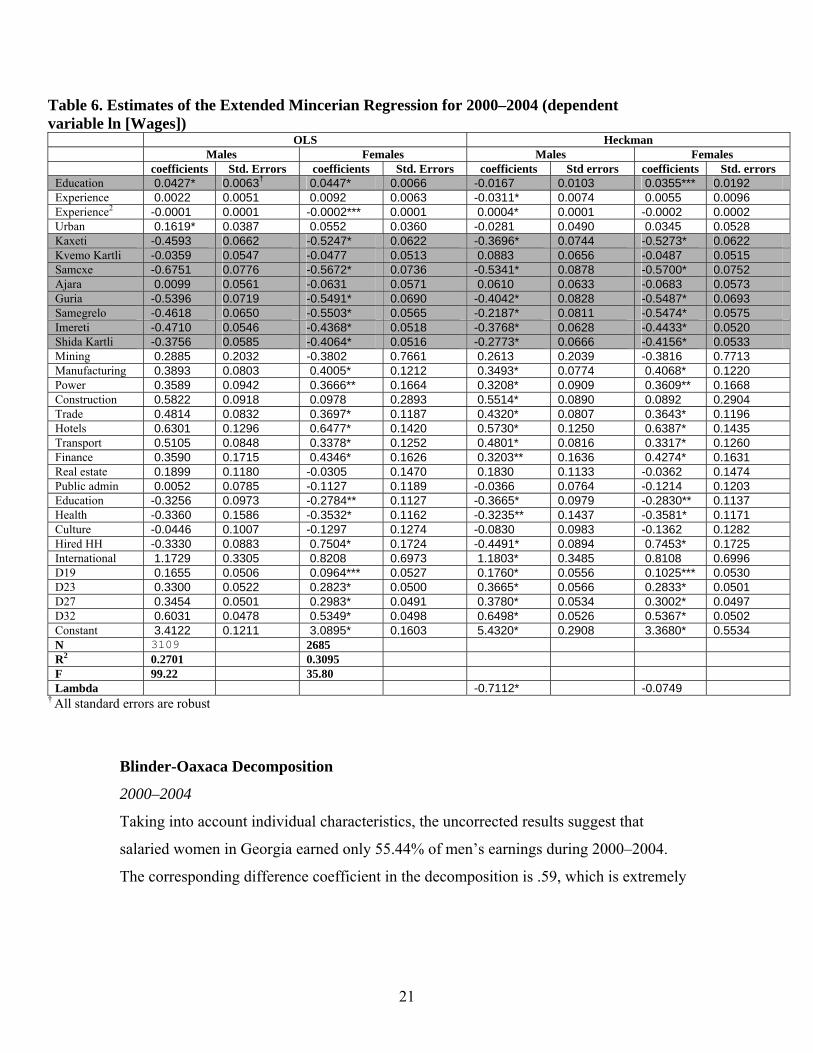
Table 6. Estimates of the Extended Mincerian Regression for 2000–2004 (dependent variable ln [Wages])

OLS Heckman Males Females Males Females coefficients Std. Errors coefficients Std. Errors coefficients Std errors coefficients Std. errors

Education 0.0427* 0.0063† 0.0447* 0.0066 -0.0167 0.0103 0.0355*** 0.0192 Experience 0.0022 0.0051 0.0092 0.0063 -0.0311* 0.0074 0.0055 0.0096 Experience2 -0.0001 0.0001 -0.0002*** 0.0001 0.0004* 0.0001 -0.0002 0.0002 Urban 0.1619* 0.0387 0.0552 0.0360 -0.0281 0.0490 0.0345 0.0528 Kaxeti -0.4593 0.0662 -0.5247* 0.0622 -0.3696* 0.0744 -0.5273* 0.0622 Kvemo Kartli -0.0359 0.0547 -0.0477 0.0513 0.0883 0.0656 -0.0487 0.0515 Samcxe -0.6751 0.0776 -0.5672* 0.0736 -0.5341* 0.0878 -0.5700* 0.0752 Ajara 0.0099 0.0561 -0.0631 0.0571 0.0610 0.0633 -0.0683 0.0573 Guria -0.5396 0.0719 -0.5491* 0.0690 -0.4042* 0.0828 -0.5487* 0.0693 Samegrelo -0.4618 0.0650 -0.5503* 0.0565 -0.2187* 0.0811 -0.5474* 0.0575 Imereti -0.4710 0.0546 -0.4368* 0.0518 -0.3768* 0.0628 -0.4433* 0.0520 Shida Kartli -0.3756 0.0585 -0.4064* 0.0516 -0.2773* 0.0666 -0.4156* 0.0533 Mining 0.2885 0.2032 -0.3802 0.7661 0.2613 0.2039 -0.3816 0.7713 Manufacturing 0.3893 0.0803 0.4005* 0.1212 0.3493* 0.0774 0.4068* 0.1220 Power 0.3589 0.0942 0.3666** 0.1664 0.3208* 0.0909 0.3609** 0.1668 Construction 0.5822 0.0918 0.0978 0.2893 0.5514* 0.0890 0.0892 0.2904 Trade 0.4814 0.0832 0.3697* 0.1187 0.4320* 0.0807 0.3643* 0.1196 Hotels 0.6301 0.1296 0.6477* 0.1420 0.5730* 0.1250 0.6387* 0.1435 Transport 0.5105 0.0848 0.3378* 0.1252 0.4801* 0.0816 0.3317* 0.1260 Finance 0.3590 0.1715 0.4346* 0.1626 0.3203** 0.1636 0.4274* 0.1631 Real estate 0.1899 0.1180 -0.0305 0.1470 0.1830 0.1133 -0.0362 0.1474 Public admin 0.0052 0.0785 -0.1127 0.1189 -0.0366 0.0764 -0.1214 0.1203 Education -0.3256 0.0973 -0.2784** 0.1127 -0.3665* 0.0979 -0.2830** 0.1137 Health -0.3360 0.1586 -0.3532* 0.1162 -0.3235** 0.1437 -0.3581* 0.1171 Culture -0.0446 0.1007 -0.1297 0.1274 -0.0830 0.0983 -0.1362 0.1282 Hired HH -0.3330 0.0883 0.7504* 0.1724 -0.4491* 0.0894 0.7453* 0.1725 International 1.1729 0.3305 0.8208 0.6973 1.1803* 0.3485 0.8108 0.6996 D19 0.1655 0.0506 0.0964*** 0.0527 0.1760* 0.0556 0.1025*** 0.0530 D23 0.3300 0.0522 0.2823* 0.0500 0.3665* 0.0566 0.2833* 0.0501 D27 0.3454 0.0501 0.2983* 0.0491 0.3780* 0.0534 0.3002* 0.0497 D32 0.6031 0.0478 0.5349* 0.0498 0.6498* 0.0526 0.5367* 0.0502 Constant 3.4122 0.1211 3.0895* 0.1603 5.4320* 0.2908 3.3680* 0.5534 N 3109 2685 R2 0.2701 0.3095 F 99.22 35.80 Lambda -0.7112* -0.0749

† All standard errors are robust

Blinder-Oaxaca Decomposition

2000–2004

Taking into account individual characteristics, the uncorrected results suggest that

salaried women in Georgia earned only 55.44% of men’s earnings during 2000–2004.

The corresponding difference coefficient in the decomposition is .59, which is extremely

22

high relative to other countries (Johnes and Tanaka 20088; Anderson and Pomfret 2003;

ADB 2005).

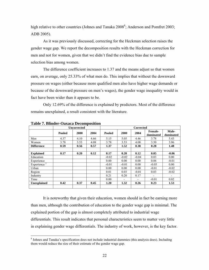
As it was previously discussed, correcting for the Heckman selection raises the

gender wage gap. We report the decomposition results with the Heckman correction for

men and not for women, given that we didn’t find the evidence bias due to sample

selection bias among women.

The difference coefficient increases to 1.37 and the means adjust so that women

earn, on average, only 25.33% of what men do. This implies that without the downward

pressure on wages (either because more qualified men also have higher wage demands or

because of the downward pressure on men’s wages), the gender wage inequality would in

fact have been wider than it appears to be.

Only 12.69% of the difference is explained by predictors. Most of the difference

remains unexplained, a result consistent with the literature.

Table 7. Blinder-Oaxaca Decomposition Uncorrected Corrected Pooled 2000 2004 Pooled 2000 2004 Female-

dominated Male-

dominated Men 4.37 4.10 4.66 5.15 5.05 4.46 3.78 5.43 Women 3.78 3.53 4.08 3.78 3.53 4.08 3.50 3.96 Difference 0.59 0.56 0.57 1.37 1.52 0.38 0.28 1.48 Explained 0.17 0.20 0.12 0.17 0.20 0.12 0.05 -0.06 Education -0.02 -0.02 -0.04 0.03 0.00 Experience 0.00 0.00 0.00 0.06 -0.01 Experience 2 -0.01 -0.01 0.00 -0.05 0.00 Urban 0.00 0.00 0.00 -0.01 -0.02 Region 0.01 0.03 -0.01 0.03 -0.02 Industry 0.21 0.20 0.17 - - Time 0.00 - - -0.01 0.02 Unexplained 0.42 0.37 0.45 1.20 1.32 0.26 0.23 1.53

It is noteworthy that given their education, women should in fact be earning more

than men, although the contribution of education to the gender wage gap is minimal. The

explained portion of the gap is almost completely attributed to industrial wage

differentials. This result indicates that personal characteristics seem to matter very little

in explaining gender wage differentials. The industry of work, however, is the key factor.

8 Johnes and Tanaka’s specification does not include industrial dummies (this analysis does). Including them would reduce the size of their estimate of the gender wage gap.

23

To gain additional insight as to within-industry wage differentials, we separate the

sample into two groups—male-dominated and female-dominated industries—and

decompose the gender wage gap for each category. We define industries in which more

than 75% of hired workers are women as female-dominated and industries in which more

than 75% of hired workers are men as male-dominated.

Education, health, and domestic household help are the three female-dominated

industries. In these industries, as expected, the gender wage gap is much smaller, at 0.28.

Out of it, 16.64% is explained. These also happen to be industries with low mean wages

(see table 2).

Six industries can be considered male-dominated: agriculture, mining, energy,

construction, transport, and public administration. In these industries, the gender wage

gap is substantial, at 1.47. Out of it, less than 0% is explained, meaning that based on the

included characteristics, women should be earning more than men, but they are not.

In interpreting the results of industry-based decompositions, we have to be

mindful of endogeneity. In our interpretation, the dominance of women in an industry

leads to less discrimination. However, one of the reasons for women not entering a

particular industry might be that they expect more discrimination in it in the first place.

Time Trends

Without the Heckman correction, in 2000 women earned 56.86% of what men did,

whereas in 2004 they earned 56.36% of what men did. Thus, without sample selection

correction, it seems that there were not changes.

The results corrected for sample selection bias however indicate a sizable drop in

the estimated gender wage gap from 1.52 in 2000 to 0.38 in 2004, still high, but a much

more “reasonable” number. These correspond to women earning 21.96% of what men

earned in 2000 and 68.57% of what men earned in 2004. The drop occurs because men’s

estimated earnings decreased during this period, whereas women’s estimated earnings

increased (the same as uncorrected results), both factors contributing to the decrease in

the estimated gender wage gap.

24

The decrease in men’s wages occurs because ρ turns positive in 2004 and, thus,

the corrected mean wages are lower than the uncorrected mean wages for that year,

indicating the “regular” reservation wage story.9

In 2000 only 13.04% of this difference was explained by predictors, whereas in

2004 a much higher 32.24% was explained by predictors.

For both 2000 and 2004, based on education alone, women should be earning

more than men. However, the most important category explaining the gender wage gap is

industrial dummy variables. That is, without industrial dummies we would be able to

explain almost none of the gender wage gap.

Blinder-Oaxaca Decomposition: Caveats and Further Analysis

In interpeting the results of this analysis and in comparing them to other studies, we must

be wary of several factors. In particular, the omission of potentially important variables

could be one factor responsible for the large degree of gender wage gap found in this

study. For example, the position in the company is one variable that can influence the

size of the estimated gender wage gap. In principle, the size of the estimated wage gap is

likely to decrease if more men hold supervisory positions (which also pay more) relative

to women. It must be kept in mind that including position as a variable is subject to the

same objections as using industrial dummies, as both variables capture aspects of

discrimination. Evidence from Georgia indicates that vertical segregation by gender is, in

fact, a common occurrence (Sumbadze 2008: 69).

Another potentially important variable is the size of the company. For example,

larger companies are presumably more visible. As a result, gender wage differentials in

these companies might be lower than they are in smaller companies. In addition, the

ownership of the company can play an important role, as private firms might have more

leeway at setting their wages and, thus, discrimination might be more prevalent. The

findings of Jurajda (2003) support this assertion.

To complement the findings of our analysis with respect to the position within

firms, firm size, and firm ownership in Georgia, we use the results of the sociological

survey conducted in Georgia in 2006 and 2007 under the UN project “Gender and

9 First-stage probit results for different years are available upon request.

25

Politics in South Caucasus.” The firms were asked to provide gender statistics, although

no questions were asked about salaries. The sample consists of 211 private firms and 11

ministries. The firms are members of the Georgian Business Federation and the Chamber

of Commerce and thus comprise a highly selective group. Although the results based on

the survey are likely to underestimate the true extent of gender inequality, they can

provide helpful insights about the representation of women at the supervisory level and

the relationship between gender inequality, firm size, and firm ownership in Georgia.

In the private sector in 2006, 38% of employees were female, however only

22.3% of the supervising positions were held by females. In 2007 the percentage of

female employees increased to 42% and the percentage of females in supervisory

positions jumped to 38.2%. Although these numbers do confirm that women are

underrepresented at the supervisory level, they compare favorably to other countries

(Jurajda 2003).10 The survey results indicate no differences in the proportion of women

represented in large firms relative to small firms. Neither does it indicate any differences

in the proportion of women between public and private firms.

Another key variable, which we haven’t included due to data limitations, is the

length of time worked, measured either as a dummy for part-time versus full-time work

or as a continuous variable representing the number of hours worked.11 According to

Weichselbaumer and Winter-Ebmer (2005), 99% of studies analyzing the gender wage

gap omit the number of hours and 51% of studies omit the part-time dummy. Brainerd

(2000) addresses the implications of not having information on the number of hours

worked. She acknowledges that if women work fewer hours than men do, which is often

the case, then the gender wage gap will be overestimated. However, without additional

information the direction of the bias is hard to predict. With respect to part-time work,

Malysheva and Verashchagina (2007) find that in most former Soviet countries the share

of part-time employment is minor, possibly indicating that omitting this variable is not

problematic.

An important avenue for future work includes the investigation of differences that

are likely to exist among different income groups, as the present study focused on the

10 Although, again, we have to be mindful of the selective nature of the survey. 11 When using hourly wages as the dependent variable, the need to include the hours of work does not arise.

26

mean wage differentials. Not only the magnitude, but the nature, of discrimination may

differ, as could be seen by looking at industrial breakdown (see Jurajda [2003] for more

on this).

Finally, future work needs to pay attention to the issue of self-employment. The

selection process occurs not only with respect to wage employment, but with respect to

self-employment, in particular for women. A growing number of studies argue for the

presence of significant differences in the nature and magnitude of the gender wage gap

between paid and self-employed workers (Eastough and Miller 2004).

CONCLUSIONS

The results of this study indicate the presence of a substantial gender wage gap in

Georgia, most of which cannot be explained by included characteristics. The component

of the wage gap that can be explained is almost completely due to occupational

differences, with the majority of the paid female labor force working in three industries:

education, health care, and culture. These also happen to be industries with the lowest

mean wages.

Yet, there are indications of positive changes, as the sample-selection-corrected

gender wage gap shrank between 2000 and 2004. During this period, industry premia for

women in high-skilled sectors, such as finance and international organizations, as well as

manufacturing and energy, increased substantially. Moreover, for women shifts occurred

within service industry away from health into education and public administration. For

men, the changes in industry premia and industrial shifts were not as pronounced.

The results of this study reflect important differences in the way in which women

have adjusted to the transition process compared to men. In some ways, the difficult

economic environment coupled with women’s caretaking responsibilities have shielded

them from experiencing more significant discrimination in the labor market. Due to

relatively few economic opportunities, men are facing stiff competition for jobs and seem

to be accepting job opportunities with wages that women might refuse, given their higher

opportunity cost of time. As a result, men’s wages are depressed and, thus, the gender

27

wage gap does not appear to be as high as it would be if we took into account the

individuals that are not observed in the sample.

The results of this study reflect important differences in the way in which women

have been affected by the transition process compared to men. It appears that women are

less likely to accept jobs with wages in the lower spectrum of their wage-offer

distribution, presumably due to their primary caretaking responsibilities. On the other

hand, among men, stiff competition for jobs, coupled with their primary responsibility as

financial providers, seem to have led to more men accepting jobs at wages in the lower

spectrum of their wage-offer distribution. As a result, especially among the less educated,

a large percentage of men are likely to remain unobserved in the sample. This leads to the

significant sample selection bias among men, which, when corrected for, raises men’s

mean wages and decreases the estimates of the education coefficient. Thus, in ironic way,

a difficult economic environment, together with women’s caretaking responsibilities,

have shielded women from experiencing more significant discrimination in the labor

market.

28

REFERENCES

Anderson, K.H., and R.W.T. Pomfret. 2003. Consequences of Creating a Market

Economy: Evidence from Household Surveys in Central Asia. Cheltenham, UK: Edward Elgar Publishing.

Arabsheibani, R., and L. Lau. 1999. “’Mind the Gap’: An Analysis of Gender Wage

Differentials in Russia.” Labour 13(4): 761–774. Arabsheibani, R., and A. Mussurov. 2007. “Returns to Schooling in Kazakhstan: OLS

and Instrumental Variables Approach.” Economics of Transition 15(2): 341–364. Asian Development Bank (ADB). 2005. “The Kyrgyz Republic, a Gendered Transition:

Soviet Legacies and New Risks.” Asian Development Bank, Country Gender Assessment, December.

Blau, F., and M.A. Ferber. 1987. “Discrimination: Empirical Evidence from the United

States.” American Economic Association Papers and Proceedings 77(2): 316–320.

Blau, F., and L. Kahn. 2000. “Gender Differences in Pay.” Journal of Economic

Perspectives 14(4): 75–99. Bodrova, V. 1993. “Glasnost and the Woman Question in the Mirror of Public Opinion:

Attitudes towards Women, Work and the Family.” in V.M. Moghadam (ed.), Democractic Reform and the Position of Women in Transitional Economies. Oxford: Oxford University Press.

Brainerd, E. 1998. “Winners and Losers in Russia’s Economic Transition.” The American

Economic Review 88(5): 1094–1116. ————. 2000. “Women in Transition: Change in Gender Wage Differentials in Eastern

Europe and FSU.” Industrial and Labour Relations Review 54(1): 139–162. Card, D. 1999. “The Causal Effect of Education on Earnings.” in O. Ashenfeleter and D.

Card (eds.), Handbook of Labor Economics, vol. 3. Amsterdam: Elsevier. ————. 2001. “Estimating the Return to Schooling: Progress on Some Persistent

Econometrics Problems.” Econometrica 69(5): 1127–1160. CEDAW. 2006. “Women’s Anti-Discrimination Committee Encourages Georgia to

Widen Scope of Efforts to Promote Gender Equality.” Post-meet report from the United Nations Committee on Elimination of Discrimination against Women’s (CEDAW) 747th and 748th meetings, August 15.

29

Cheidvasser, S., and H. Benitez-Silva. 2007. “The Educated Russian’s Curse: Returns to Education in the Russian Federation During the 1990s.” Labour 21(1): 1–41.

Department of Statistics. 2006. Georgian Statistical Yearbook. Tbilisi: Georgian

Department of Statistics, Ministry of Economic Development. ————. 2008. Women and Men in Georgia: Statistical Booklet. Tbilisi: Department of

Statistics, Ministry of Economic Development. Dolado, J., F. Felgueroso, and J.F. Jimeno. 2002. “Recent Trends in Occupational

Segregation by Gender: A Look across the Atlantic.” Working Paper No. 02-30. Madrid: Universidad Carlos III de Madrid.

Dolton, P.J., and G.H. Makepeace. 1986. “Sample Selection and Male-Female Wage

Differentials in the Graduate Labour Market.” Oxford Economic Papers 38(1): 317–341.

Dougherty, C. 2003. “Why is the Rate of Return to Schooling Higher for Women than for

Men?” Discussion Paper No. 581. London: Centre for Economic Performance, London School of Economics and Political Science.

Eastough, K., and P.W. Miller. 2004. “The Gender Wage Gap in Paid- and Self-

Employment in Australia.” Australian Economic Papers 43(3): 257–276. Ermisch, J.F., and R.E. Wright. 1994. “Interpretation of Negative Sample Selection

Effects in Wage Offer Equations.” Applied Economics Letters 94(1): 187–189. Gerry, C. J., B. Kim, and C.A. Li. 2004. “The Gender Wage Gap and Wage Arrears in

Russia: Evidence from the RLMS.” Journal of Population Economics 17(2): 267–288.

Glinskaya, E., and T.A. Mroz. 2000. “The Gender Gap in Wages in Russia from 1992 to 1995.” Journal of Population Economics 13: 353–386.

Guarcello, L., S. Lyon, F.C. Rosati, and C. Valdivia. 2005. “School to Work Transitions

in Georgia: A Preliminary Analysis Based on Household Budget Survey Data.” Working Paper 23. Rome: UNICEF (Understanding Children’s Work Project).

Harmon, C., and I. Walker. 1995. “Estimates of the Economic Return to Schooling for

the UK.” American Economic Review 85(5): 1279–1286. Heckman, J. 1979. “Sample Selection Bias as a Specification Error.” Econometrica

47(1): 153–161. Hundley, G. 2000. “Male/Female Earnings Differences in Self-Employment: The Effects

of Marriage, Children, and the Household Division of Labor.” Industrial and Labor Relations Review 54(1): 95–114.

30

Jann, B. 2008. “The Blinder-Oaxaca Decomposition of Linear Models.” Stata Journal 8(4): 453–479.

Jashi, C. 2005. Gender Economic Issues: The Case of Georgia. Tbilisi: UNDP/SIDA. Jolliffe, D. 2002. “The Gender Wage Gap in Bulgaria: A Semiparametric Estimation of

Discrimination.” Journal of Comparative Economics 30: 276–295. Johnes, G., and Y. Tanaka. 2008. “Changes in Gender Wage Discrimination in the 1990s:

A Tale of Three Very Different Economies.” Japan and the World Economy 20(1): 97–113.

Jurajda, S. 2003. “Gender Wage Gap and Segregation in Enterprises and the Public

Sector in Late Transition Countries.” Journal of Comparative Economics 31(2): 199–222.

Kazakova, E. 2007. “Wages in a Growing Russia: When is a 10 Per Cent Rise in the

Gender Wage Gap Good News?” Economics of Transition 15(2): 365–392. Khitarishvili, T. 2008. “Environment for Human Capital Accumulation: The Case of

Georgia.” Unpublished manuscript. Lauerova, J.S., and K. Terrell. 2002. “Explaining Gender Differences in Unemployment

with Micro Data on Flows in Post-Communist Economies.” Discussion Paper No. 600. Bonn: Institute for the Study of Labor.

Malysheva, M., and A. Verashchagina. 2007. “The Transition from Planned to Market

Economy: How are Women Fairing?” in F. Bettio and A. Verashchagina (eds.), Frontiers in the Economics of Gender. London and New York: Routledge Siena Studies in Political Economy.

Mincer, J. 1974. Schooling, Experience and Earnings. New York: National Bureau of

Economic Research. Newell, A., and B. Reilly. 1996. “The Gender Wage Gap in Russia: Some Empirical

Evidence.” Labour Economics 3(3): 337–356. Nicaise, I. 2001. “Human Capital, Reservation Wages, and Job Competition: Heckman’s

Lambda Reinterpreted.” Applied Economics 33(3): 309–315. Ofer G., and A.Vinokur. 1992. The Soviet Household under the Old Regime: Economics

Conditions and Behaviour in the 1970s. Cambridge: Cambridge University Press. Pastore F., and A. Verashchagina. 2007 “When Does Transition Increase the Gender

Wage Gap? An Application to Belarus.” Discussion Paper No. 2796. Bonn: Institute for the Study of Labor.

31

Reilly, B. 1999. “The Gender Pay Gap in Russia during the Transition, 1992–1996.” Economics of Transition 7(1): 245–264.

Sabedashvili, T. 2007. “Gender and Democratization: The Case of Georgia 1991–2006.”

Tbilisi: Heinrich Boll Foundation, South Caucasus Regional Office. Schultz, T.P. 1993. “Investments in the Schooling and Health of Women and Men:

Quantities and Returns.” Journal of Human Resources 28(4): 694–734. Sumbadze, N. 2008. Gender and Society. Tbilisi: Institute of Policy Studies, UNDP

Project “Gender and Politics.” Weichselbaumer, D., and R. Winter-Ebmer. 2005. “A Meta-Analysis of the International

Gender Wage Gap.” Journal of Economic Surveys 19(1): 479–511. Yemtsov, R. 2001. “Labor Markets, Inequality and Poverty in Georgia.” Discussion

Paper No. 251. Bonn: Institute for the Study of Labor.

32

APPENDIX Table A1. Description of the Variables Variable Description Gender 0 – male; 1 – female Marriage 0 – not married, divorced, or widowed; 1 – registered marriage, non-registered

marriage, or separated (married) Regional Dummies 1 if region = the region of interest, 0 otherwise

Urban or Rural 0 – rural, 1 – urban Branch of Employment

1 – agriculture, forestry, fishing 2 – mining and quarrying 3 – manufacturing 4 – power, gas, and water supply 5 – construction 6 – trade and repair of domestic appliances 7 – hotels and restaurants 8 – transport, storage, and communications 9 – financial intermediation 10 – transactions with real estate, leasing, and R&D 11 – public administration 12 – education 13 – health care and social services 14 – other services, culture, entertainment, and recreation 15 – hired services in households 16 – extraterritorial (international) organizations

Table A2. Female Paid Labor Force Composition by Industry 2000 2001 2002 2003 2004 Agriculture 1.17 0.97 1.28 2.44 1.52 Mining 0.00 0.48 0.37 0.15 0.00 Manufacturing 6.44 7.25 5.69 8.09 7.12 Power 1.02 1.77 2.39 2.90 0.76 Construction 0.15 0.48 0.55 0.31 0.30 Trade 11.42 9.18 9.91 8.70 9.70 Hotels 1.46 2.74 3.67 2.29 3.18 Transport 4.25 3.70 4.40 3.82 4.39 Finance 2.78 2.74 1.83 1.68 2.27 Realestate 3.07 2.58 2.57 3.51 4.09 Publicadmin 6.59 12.40 10.09 8.70 9.85 Educations 33.67 33.33 35.60 35.42 36.67 HealthS 21.38 16.59 15.78 14.05 13.03 Culture 5.86 5.64 5.32 6.72 5.61 HiredHH 0.44 0.00 0.55 0.92 0.91 International 0.29 0.16 0.00 0.31 0.61

33

Table A3. Male Labor Force Composition by Industry 2000 2001 2002 2003 2004 Agriculture 3.64 4.18 4.59 8.64 8.82 Mining 1.04 0.28 1.15 0.81 1.12 Manufacturing 15.21 14.92 15.41 13.09 13.31 Power 6.76 6.28 7.05 6.21 5.60 Construction 6.11 4.60 5.74 6.88 7.28 Trade 10.66 9.34 10.16 12.55 10.64 Hotels 1.95 2.37 1.31 0.27 1.45 Transport 12.61 13.53 12.79 10.53 9.52 Finance 1.69 1.12 0.82 1.35 1.40 Realestate 4.29 2.23 2.13 4.72 4.20 Publicadmin 19.12 24.41 22.95 21.73 20.31 Educations 7.54 9.34 6.89 6.21 7.28 HealthS 4.03 2.93 3.77 2.16 2.66 Culture 5.07 4.46 5.08 4.45 5.46 HiredHH 0.26 0.00 0.00 0.00 0.00 International 0.00 0.00 0.16 0.40 0.84