January 2016

Working paper

POLICY AND MACRO SIGNALS AS INPUTS TO INFLATION EXPECTATION FORMATION

Paul HUBERT OFCE-Sciences Po

Becky MAULE

Bank of England

2016

-02

1

Policy and Macro Signals as Inputs to Inflation Expectation Formation*

Paul Hubert OFCE - Sciences Po

Becky Maule Bank of England

January 2016

Abstract How do private agents interpret central bank actions and communication? To what extent do the effects of monetary shocks depend on the information disclosed by the central bank? This paper investigates the effect of monetary shocks and shocks to the Bank of England’s inflation and output projections on the term structure of UK private inflation expectations, to shed light on private agents’ interpretation of central bank signals about policy and the macroeconomic outlook. We proceed in three steps. First, we correct our dependent variables – market-based inflation expectation measures – for potential risk, liquidity and inflation risk premia. Second, we extract exogenous shocks following Romer and Romer (2004)’s identification approach. Third, we estimate the linear and interacted effects of these shocks in an empirical framework derived from the information frictions literature. We find that private inflation expectations respond negatively to contractionary monetary policy shocks, consistent with the usual transmission mechanism. In contrast, we find that inflation expectations respond positively to positive central bank inflation or output projection shocks, suggesting private agents put more weight on the signal that they convey about future economic developments than about the policy outlook. However, when shocks to central bank inflation projections are interacted with shocks to output projections of the same sign, they have no effect on inflation expectations, suggesting that private agents understand the functioning of the central bank reaction function and put more weight on the policy signal when there is no trade-off. We also find that the effects of contractionary monetary shocks are amplified when they are accompanied by positive shocks to central bank inflation projections. The coordination of policy decisions and macroeconomic projections thus appears important for managing inflation expectations. Keywords: Monetary policy, information processing, signal extraction, market-based

inflation expectations, central bank projections, real-time forecasts. JEL codes: E52, E58.

                                                            * We thank Christophe Blot, James Cloyne, Camille Cornand, Jérôme Creel, Martin Ellison, Rodrigo Guimarães, Refet Gürkaynak, Stephen Hansen, Frédéric Jouneau-Sion, Michael McMahon, Jon Relleen, Garry Young and seminar participants at the GATE, Bank of England, OFCE, European Central Bank, Deutsche Bundesbank, CEPII, the Workshop on Empirical Monetary Economics 2015, the Workshop on Probabilistic Forecasting and Monetary Policy, GDRE 2015, the Central Bank Design workshop of the 2015 BGSE Summer Forum, the 2015 World Congress of the Econometric Society and AFSE 2015 for their comments at different stages of this project. We also thank Simon Strong for research assistance. Paul Hubert thanks the Bank of England for its hospitality. Any remaining errors are our own responsibility. Any views expressed are solely those of the authors and so cannot be taken to represent those of the Bank of England or members of the Monetary Policy Committee or Financial Policy Committee or to state Bank of England policy. Corresponding author: paul.hubert@sciencespo.fr. Tel: +33144185427. Address: OFCE, 69 quai d’Orsay, 75007 Paris, France.

2

1. Introduction Expectations matter in determining current and future macroeconomic outcomes. Hence, the management of private expectations has become a central feature of monetary policy (Woodford, 2005), as private agents’ interpretation of central bank decisions and communication is crucial in the formation of their beliefs. In a set-up with information frictions, both the central bank’s decisions and its economic projections can convey information about its view on both macroeconomic developments and about current and future policy developments. The former channel arises from the fact that private agents might have different information sets to the central bank. In that case, the central bank’s policy decisions and its communication about its view of macroeconomic developments can signal that information to private agents, influencing their beliefs about the economic outlook. We define this as a ‘macro outlook signal’. The latter channel stems from the central bank’s ability to affect real variables through the real interest rate because of nominal rigidities or information frictions. Because of this, a central bank’s policy decisions and projections for the economy can also provide private agents with information about the outlook for policy. We define this as a ‘policy signal’.1 Which channel – the macro outlook or policy signal – dominates matters, given that the transmission of monetary policy depends on how private agents interpret changes in the policy rate or in central bank projections. For instance, on the one hand, an increase in the policy rate could signal to private agents that an inflationary shock will hit the economy in the future, causing higher inflation. On the other hand, the same increase in the policy rate may be interpreted as a simple contractionary monetary shock, which will lead to lower inflation in the future. If the first interpretation is given more weight, then increasing the policy rate will lead to higher private inflation expectations, whereas if the second is, then tightening the policy rate will decrease private inflation expectations.2 Similarly, an increase in the central bank’s inflation projections could signal to private agents that an inflationary shock will hit the economy in the future, causing higher inflation; whereas the same increase in central bank inflation projections may be interpreted as a signal about a future policy tightening, which will lead to lower expected inflation. This paper assesses, for the United Kingdom (UK), whether and how the term structure of market-based inflation expectations responds to policy decisions and central bank macroeconomic projections, and so which signal dominates.3 If a positive signal about the macro outlook is taken from either a policy decision or a change in the central bank’s economic projections, inflation expectations will increase. Whereas if either a higher policy setting or economic projections is taken to signal a future contractionary policy shock, inflation expectations will decrease. Hence, a policy signal being taken will have the opposite effect on inflation expectations to the circumstance in which a macro outlook signal is taken, and so the sign of the estimated effects of shocks to Bank Rate and the Bank of England

                                                            1 We use the term ‘policy signal’ for the classical monetary transmission channel and the term ‘macro outlook signal’ for what Melosi (2015), for instance, calls the ‘signaling channel of monetary policy’. That is because we study the information content of a central bank’s macroeconomic projections (as well as its policy decisions), so the usual terminology is not appropriate. 2 The macro outlook signal of monetary policy shocks might then be one of the explanations for the positive response of inflation to monetary shocks documented in the VAR literature as the “price puzzle” (Sims 1992). Castelnuovo and Surico (2010) finds that including inflation expectations in VARs captures this price puzzle, so evidence supporting the possibility of an outlook signal would reconcile these contributions. 3 We specifically focus on quantitative communication so as to abstract from quantification issues of other types of qualitative communication like statements, minutes and speeches (see Blinder et al. 2008 for a review).

3

(Bank hereafter)’s macroeconomic projections on private inflation expectations is indicative of the relative weight private agents put on each signal. We then investigate whether the publication of macroeconomic projections, by facilitating information processing, modifies private agents’ signal extraction from monetary shocks. The literature has focused, both theoretically and empirically, on the classical monetary policy transmission signal, while the macro signalling issue has received less attention – most of the analyses that do exist are theoretical in nature. For example, Morris and Shin (2002) show that public signals – for instance those from a central bank – affect private agents’ actions. And Angeletos et al. (2006) study the signalling effects of policy in a coordination game. Walsh (2007) studies optimal transparency when the central bank provides public information by setting its policy instrument. In Baeriswyl and Cornand (2010), the central bank instrument discloses information about policymakers’ assessment of shocks which are imperfectly observed by firms. Kohlhas (2014) shows how central bank information disclosure may increase the information content of public signals about the state of the economy. Tang (2014) builds a model in which policy actions can signal information about macro developments, because policymakers are more informed than private agents about exogenous shocks. Melosi (2015) develops a model in which the policy rate has signalling effects about the macro outlook because aggregate variables are not observed by individual firms. Nevertheless, none of these works investigates the signals that can be taken – about the policy and macro outlook – from central bank macroeconomic projections. This work is also related to the empirical finding documented by Romer and Romer (2000), Campbell et al. (2012), Nakamura and Steinsson (2013) that contractionary United States’ federal fund rate surprises can have, under certain conditions, positive effects on private inflation or output expectations.4 The contribution of this paper is to bring the issue of the signals provided by monetary shocks to the data, and to extend the analysis to the signals provided by central bank macroeconomic projections. Facilitating private agents’ information processing has been put forward as one reason why central banks complement their actions with communication (Gürkaynak et al. 2005, and Reis 2013), and we aim to document this potential interdependence. Our empirical analysis proceeds in three steps. First, we correct our dependent variables, UK market-based inflation expectation measures, for risk, liquidity and inflation risk premia following the methodology used by Gürkaynak et al. (2010a, 2010b) and Soderlind (2011). Second, we deal with the issue of endogeneity by extracting series of exogenous shocks to the Bank’s policy rate and inflation and output projections by removing their systematic component, following the identification methodology of Romer and Romer (2004) and applied to UK data by Cloyne and Huertgen (2014) to derive a narrative monetary policy shock series. In the potential presence of non-nested information sets, we augment the Romer and Romer (2004)’s approach so that exogenous shocks are not only orthogonal to the                                                             4 This paper also refers to a large literature focusing on the expectation formation process departing from the full-information rational expectation hypothesis, introducing information frictions to account for some empirical regularities about the persistence of private expectations (sticky information, noisy information or adaptive learning models, and classes of models with heterogeneity in beliefs or in loss functions) led by Evans and Honkapohja (2001), Bullard and Mitra (2002), Mankiw and Reis (2002), Sims (2003), Orphanides and Williams (2005, 2007) and Branch (2004, 2007). Another strand of the literature tries to explain macroeconomic outcomes with expectations data (see e.g. Nunes 2010 and Adam and Padula 2011), while another strand focuses on the characteristics, responsiveness to news, dispersion or anchoring of expectations (see e.g. Gürkaynak et al. 2005, Swanson 2006, Capistran and Timmermann 2009, Crowe 2010, Gürkaynak et al. 2010a, Beechey et al. 2011, Coibion and Gorodnichenko 2012, 2015, Dräger and Lamla 2013, Ehrmann 2014, Hubert 2014, 2015).

4

central bank’s information set but also to private agents’ information set: Blanchard et al. (2013) and Miranda-Agrippino and Ricco (2015) discuss how information frictions modify the econometric identification problem. Third, we estimate the individual and interacted effects of these exogenous shocks in a general empirical framework derived from the information frictions literature, controlling for private output and interest rate expectations and for inflation surprises. We find that private inflation expectations respond negatively to contractionary monetary shocks but positively to central bank inflation and output projections. The sign of the effect of the Bank’s projections on inflation expectations indicates that private agents take a greater signal about the macro outlook from those projections than they do about the outlook for policy. That provides tentative evidence of the existence of a macro outlook signalling channel, in contrast to the theoretical predictions of full information models. More generally, one interpretation is that when private agents face a signal extraction problem from one shock only, they rely on the underlying nature of the information disclosed by the central bank: a monetary shock primarily conveys a policy signal and a projection shock primarily conveys a macro signal. We find that a positive shock to the Bank’s inflation projections has no effect on private inflation expectations when interacted with a positive shock to the Bank’s output projections, even though both projections individually have a positive effect. That suggests that the weight put on the policy signal from each shock is increased when both occur together. That might suggest that private agents understand the trade-off inherent in a central bank’s reaction function, and so are able to anticipate the likely endogenous policy response when that trade-off does not occur. In contrast, when the shocks to inflation and output projections have opposite signs, a positive shock to the Bank’s inflation projections has a positive effect on private inflation expectations. That is consistent with the macro outlook signal dominating the policy signal because the policy response is less clear. Finally, we find that shocks to the Bank’s inflation projections affect the impact of monetary shocks on inflation expectations. A positive shock to Bank Rate – i.e. a contractionary monetary shock – has a more negative effect on inflation expectations when it is interacted with a positive shock to the Bank’s inflation projections, whereas it has no effect when it is interacted with a negative shock to the Bank’s inflation projections. This suggests that the policy signal taken from a monetary shock is given a stronger weight when the shock is corroborated by information about the central bank’s view of the macroeconomic outlook. The same is not true of shocks to the Bank’s output projections, although that might be consistent with the remit of an inflation targeting central bank. These results give policymakers some insights on how private agents interpret and respond to policy decisions and central bank information. The signals provided by central bank action and communication appear to be important for the management of private inflation expectations, and these findings suggest that the publication of macroeconomic projections helps private agents’ information processing. The rest of the paper is organised as follows. Section 2 describes the theoretical and empirical framework, section 3 the data, section 4 the correction of our dependent variables for different premia, section 5 the first stage regression to extract exogenous shocks from our independent variables, and section 6 the estimates. Section 7 concludes.

5

2. Framework This section sets out our approach. First, we use insights from the literature to derive predictions about how private inflation expectations might react to shocks to the monetary stance and the Bank’s inflation and output projections under different assumptions about private agents’ information sets. Second, we develop an empirical specification, based on assumptions about private agents’ inflation expectations formation process, which allows us to test which of those predictions appear to hold for UK data. 2.1. Theoretical predictions First, we derive predictions for the expected effects of shocks to policy decisions and central bank macroeconomic projections on private inflation expectations based on a standard macroeconomic framework, assuming all agents have full information. We base those on the effects that result from a standard 3-equation New-Keynesian (NK) model à la Rotemberg and Woodford (1997), augmented with habits in consumption and a Calvo price-setting mechanism as in Clarida, Gali and Gertler (1999). In such a framework, contractionary monetary shocks have a negative effect on private inflation expectations, through the usual transmission channels. Moreover, positive shocks to the central bank’s projections also have a negative effect on private inflation expectations. That is because shocks to projections enter the Taylor rule and are interpreted only as signals about future policy reactions, and a higher inflation projection leads agents to anticipate higher nominal interest rates in future. In a framework with full information, monetary or projection shocks are perfectly observed and there is no room for signals about the macroeconomic outlook. So, in a model with nested information sets, we would predict that both contractionary shocks to Bank Rate and positive shocks to the Bank’s inflation or output projections would negatively affect private inflation expectations. Those predictions are shown in the first column of Table 1. Second, we derive predictions for the expected effects of the shocks under a framework in which private agents and the central bank have non-nested information sets. That assumption would be consistent with works by Coibion and Gorodnichenko (2012, 2015) and Andrade and Le Bihan (2013), which provide empirical evidence of rejection of full information models. In addition, recent works on rational expectation models with information frictions such as Woodford (2001), Mankiw and Reis (2002), and Sims (2003) have highlighted how departing from the assumption of full information can account for empirical patterns about expectations, as well as leading to policy recommendations different from those with full information. In such a situation, when the observed policy rate differs from private agents’ expectations, agents cannot infer whether the central bank has changed its own view of future inflation and output or whether there has been a monetary shock. Shocks to the policy rate may therefore convey signals about both future macroeconomic developments and the policy stance to private agents. In a similar fashion, shocks to the central bank’s macroeconomic projections can also convey information about both the macro outlook as well as the future policy stance. So, in a framework with non-nested information sets, private agents face a multidimensional signal processing problem: they could take either of two signals – one about macro developments and one about future policy – from one observable variable. Said differently, private agents can misperceive changes in policy or projections for a mix of shocks in the

6

economy, which gives room for macro or policy signals – as modelled by Melosi (2015) for policy decisions.5 Those two signals would be expected to have different implications for private inflation expectations though. If either a higher policy setting or economic projections is taken to signal a future contractionary policy shock, inflation expectations will decrease. In that case, the policy signal dominates the macro outlook signal – as shown in the second column of Table 1. In contrast, if a strong positive signal about the macro outlook is taken from either a policy decision or a change in the central bank’s economic projections, inflation expectations will increase. In that case, the macro outlook signal outweighs the policy signal – as shown in the third column of Table 1.

The rest of the paper aims to investigate which predictions the UK data appear to support. The simple sign-identification strategy outlined in Table 1 allows us to assess whether there is any evidence of a macro signal, and so to assess whether private agents and central banks do have non-nested information sets. It also allows us to infer the relative weight given to each signal based on the movement in private inflation expectations. 2.2. Empirical strategy Two theoretical models with rational expectations and information frictions, in which private agents face limitations in the acquisition and processing of information, motivate our empirical setup. This subsection presents a simple and general inflation expectation formation process in which we are agnostic about whether information is imperfect or not and let the data speak. When departing from full information rational expectations, new information may be only partially absorbed over time by private agents for two reasons: either information is sticky or imperfect. In the sticky information model of Mankiw and Reis (2002), private agents update  their information set infrequently as they face costs of absorbing and processing information. However, if private agents update their information set, they gain perfect information (PI). Similarly, Carroll (2003) suggests that professional forecasts – which are assumed to be updated every period – spread epidemiologically to other private agents. Both processes can be described by these equations respectively:

, = (1-μPI) , + μPI , (1)

, = (1- μSPF) , + μSPF , (2) where , is the private inflation expectation made in period t for horizon h, , the perfect information forecast, and , the professional forecast. Private inflation expectations are                                                             5 Developing a theoretical model in which policy actions signal central bank’s information about macroeconomic developments (as in Melosi 2015, or Tang 2014) is beyond the scope of this paper, which contribution is empirical.

Policy signal > Macro signal

Macro signal > Policy signal

Monetary shock - - +

Projection shock - - +

Non-nested information setsNested information

sets

Table 1 - Expected sign of the response of inflation expectations

7

represented as a linear combination of lagged private expectations of agents who did not update their information set, and either a rational or boundedly rational forecast of the proportion μPI or μSPF of agents having updated their information set. In the noisy information models of Woodford (2001) and Sims (2003), private agents continuously update their information set but observe only noisy signals about the true state of the economy. Their observed inertial reaction arises from the inability to pay attention to all the information available. It is an optimal choice for private agents – internalizing their information processing capacity constraints – to remain inattentive to a part of the available information because incorporating all noisy signals is impossible (Moscarini 2004). In such a model, forecasts are formed via a Kalman filter and are a weighted average of agents’ prior beliefs and the new information received. They can be represented by:

, = (1-ξ) , + ξ Πt (3)

where , is a weighted average of the past inflation expectations ( , ) and of new information about future inflation summarized by the vector Πt. When the signal perfectly reveals the true state, ξ=1; when it is noisy, ξ<1. Another interpretation of this reduced-form equation is that private agents have an initial belief about future inflation (their past inflation expectations) at the beginning of each period, and during each period, they incorporate relevant - but potentially noisy - information about future inflation. We can bridge the two different strands of the literature in a simple and general equation by modelling private inflation forecasts as a linear combination of past inflation forecasts ,

and a vector Λt, which captures new information between t-1 and t. To do that, we explicitly assume private agents have homogeneous inflation forecasts in the case of sticky information models, which allows us to match the point forecasts nature of the data used hereafter:6

, = β0 + β1 , + βΛ Λt + εt (4)

The value of the β1 parameter, which we expect to be positive and significant, should shed light on whether the limited adjustment mechanism in which information is only partially absorbed over time is at work in data. The vector Λt includes the exogenous components of Bank Rate, the Bank’s inflation and output projections, as well as two additional vectors.7 The first one Xt comprises the change between t-1 and t in private output forecasts, to control for their link with private inflation forecasts as evidenced by Fendel et al. (2011), Dräger et al. (2015) and Paloviita and Viren (2013). It also includes the change between t-1 and t in private interest rate forecasts orthogonal to Bank Rate. That allows us to control for the part of interest rate expectations which is unrelated to Bank Rate, to isolate the effect of policy decisions from the effect of changes in beliefs about the transmission mechanism. Xt includes a news variable capturing the set of macroeconomic data released between t-1 and t based on the announcement literature (see Andersen et al., 2003). The second vector, Zt, includes macroeconomic variables that are likely to affect future inflation and therefore to be used by private forecasters to predict future inflation: CPI, industrial production, oil prices, sterling

                                                            6 We acknowledge that point forecasts may suffer an aggregation bias because agents may have heterogeneous beliefs due to differences in their own information sets, but we abstract from this issue in this paper. 7 For simplicity, we hereafter consider output growth forecasts, as available from the Bank of England or surveys, rather than output gap forecasts.

8

effective exchange rate, net lending, housing prices, the FTSE index and a dummy for Forward Guidance.8 Thus, equation (4) can be written as:

, = β0 + β1 , + β2 + β3 + β4 + βX Xt + βZ Zt + εt (5)

where , and are the monetary and projection shocks that we explicitly incorporate in private agents’ forecasting function. This specification can be interpreted through the lens of either noisy information models or augmented sticky-information models where rational or professional forecasts are substituted with monetary and projection shocks and additional control variables. The timing of policy decisions and Bank projection releases – made public at the beginning of the relevant months – should ensure that their information content is not already contained in private inflation expectations and that inflation expectation dynamics are not responsible for shocks. We test the robustness of this assumption by considering only the last daily observation of each month for our left-hand side variable so as to remove any potential endogeneity issue. After having corrected our dependent variables for potential risk, liquidity and inflation risk premia, and extracted exogenous shocks from our three variables of interest, we estimate equation (5) with OLS for the term structure of inflation expectations.9 The sign of the β2-β4 parameters should shed light on whether monetary and projection shocks convey a macro signal: if that dominates, the parameters will be positive effect; if the policy signal does, they will be negative. Later, we introduce interaction terms between these shocks to assess whether the effects of a given shock change when they combine with another shock. 3. Data Our dependent variable, πPF, is derived from inflation swaps. These instruments are financial market contracts to transfer inflation risk from one counterparty to another. In the UK, they are linked to the Retail Price Index (RPI) measure of inflation, rather than Consumer Price Index (CPI), which is the measure the Bank’s inflation target is currently based on. In general, the advantage of financial market expectations over survey measures of expectations is that they are directly related to payoff decisions, so there is no strategic response bias or no difference between stated and actual beliefs. Although one disadvantage is that financial market expectations do not provide a direct measure of inflation expectations as they are affected by credit risk, liquidity and inflation risk premia. Swaps tend to be a better market measure for deriving inflation expectations than index-linked gilts because they are generally less sensitive to liquidity and risk premia.

                                                            8 The Monetary Policy Committee has provided guidance on the setting of future monetary policy since 7 August 2013. For details, see http://www.bankofengland.co.uk/monetarypolicy/Pages/forwardguidance.aspx. 9 Estimating the equation along the term structure allows us to assess whether shocks have different effects at different horizons. Shocks’ signalling content (macro or policy) may vary with horizons for a number of reasons. One might relate to lags in the transmission of policy. For example, the term structure could be thought of as being split into three groups: (i) the short term (i.e. 1 year ahead), which, given the lags associated with the transmission of monetary policy, should be unaffected by changes in Bank Rate, (ii) the medium term (i.e. 2-4 years ahead), when interest rates are generally thought to affect the economy, and (iii) the long term (i.e. ≥ 5 years ahead), when the impact of any monetary shocks should have died out.

9

Another advantage of market measures is that they are available at a high frequency and for all horizons from 1 to 10 years ahead. We use them at the monthly frequency by taking the average of all the working day observations in each month.10 These are available since October 2004, which determines the starting date of our sample. For robustness purposes, we also use survey data from Citigroup/YouGov and the Survey of External Forecasters. The Bank's policy interest rate, i, called Bank Rate, is the intended policy target rate, which previously was also referred to as Minimum Lending Rate, Repo Rate, or Official Bank Rate. We also focus on the Bank’s inflation and output projections, πBoE and xBoE respectively. They are available from the quarterly Inflation Report (IR) for each quarter up to three years ahead. They are released in February, May, August and November. Two sets of forecasts are published: one set is conditioned on a constant interest rate path which ex-post includes the effect of the Monetary Policy Committee’s (MPC) most recent Bank Rate decision. The other set is conditioned on the path for Bank Rate implied by market interest rates just prior to the previous policy meeting. A crucial assumption to ensure identification is that forecasts do not already contain the effect of the policy decision (in other words, they are uncorrelated with Bank Rate) as if the forecasts included the effect of the policy change, the regression results would be biased. We therefore use the latter set of forecasts. The vector Xt includes private output forecasts obtained from Consensus Forecasts for horizons from 1 to 6 quarters ahead (monthly constant-interpolated from surveys in March, June, September and December) and from the Bank’s Survey of External Forecasters for horizons from 2 to 3 years ahead (monthly constant-interpolated from surveys in February, May, August and November). Private interest rate forecasts are 3-month market interest rate expectations derived from nominal government bonds 1 to 10 years ahead. The news variable πs represents inflation surprises: the information set of macroeconomic data released between t-1 and t having an impact on the inflation outcome. Following the announcement and news literature (Andersen et al., 2003, and references within), this variable is defined as the difference between the actual value of inflation in t and the private inflation forecast formed at date t-1 for the quarter t (πs = πt – Et-1πt). This is equivalent to the private inflation forecast error and captures the news published between the two dates. Bloomberg provides the market average expected one month ahead inflation outturn at a monthly frequency. The vector Zt comprises various macroeconomic controls that are likely to capture expected inflation dynamics: CPI inflation, industrial production, oil prices, net lending, the sterling ERI, housing prices, the FTSE index (all included as 12-month percentage changes), and a Forward Guidance dummy. Our overall sample period is 2004m10-2015m03. Data sources and descriptive statistics together with the correlation structure of our main variables of interest are presented in Tables A1 and A2 in the Appendix. 4. Correcting Market-based Expectation Measures We aim to derive more accurate estimates of market-based measures of inflation expectations by correcting inflation compensation, as measured by inflation swaps, for credit risk, liquidity and inflation risk premia. Market-based measures of inflation compensation are an

                                                            10 Since market-based inflation expectations are available at the daily frequency, the Bank’s macro projections and some of the private output forecasts at the quarterly frequency and most of the macroeconomic variables at the monthly frequency, we perform our empirical analysis at the monthly frequency. Given that we are primarily interested in the lower-frequency effects of these shocks on private inflation expectations, we chose not to perform event-study analysis at a daily frequency around policy decision and projections publication dates.

10

appropriate indicator of inflation expectations if investors are risk neutral and there is no liquidity premium. However, that is unlikely to be the case, and these premia might have sizable values and be time-varying. We use a model-free regression approach to correct our compensation measure, rather than a no arbitrage approach based on term-structure models. Gürkaynak et al. (2010a, 2010b) and Soderlind (2011) decompose inflation compensation –

, – obtained from financial market variables into: expected inflation, , , a liquidity premium, , , that investors demand to encourage them to hold these assets when they are illiquid, and an inflation uncertainty premium, , , that compensates investors for bearing inflation risk. We also include a risk premium, , , compensating investors for holding a risky asset.11 As done previously, assuming t is the time subscript and h is the horizon of inflation expectations, this breakdown can be written:

, = , + , + , + , (6)

We assume that inflation compensation is the sum of expected inflation and the different premia, and estimate a linear regression model of inflation compensation on proxy measures capturing the different premia. In the spirit of Chen, Lesmond and Wei (2007) who control for risk premium using bond ratings, the credit risk premium is proxied by the Libor-OIS spread and by the average of UK major banks’ CDS premia. Those measures should capture the riskiness of holding financial instruments, especially during the global financial crisis. The liquidity premium is proxied by the FTSE Volatility index (the UK-equivalent of the VIX), following Gürkaynak et al. (2010b) and Soderlind (2011). 12 For the inflation risk premium, we use the implied volatility from swaptions – options on short-term interest rate swaps – maturing in 20 years which captures inflation uncertainty, following Soderlind (2011).13 This leads us to estimate the following equation:

, = + spread + cds + ftsev + impvol + , (7)

We estimate equation (7) using OLS. We use monthly observations – calculated simply as the average of daily observations. And we estimate it separately for each horizon of inflation compensation from 1 year ahead to 10 years ahead. The risk premium, the liquidity premium and the inflation risk premium – which is directly related to inflation uncertainty – should

                                                            11 The credit risk premium has been neglected in most of the literature so far for two reasons. First, most of the studies focus on US treasury bonds and TIPS, and therefore implicitly assume there is no credit risk, those bonds being considered as risk-free (see Gürkaynak et al. 2010b). Second, when considering swap contracts to derive inflation expectations, the collateral is supposed to remove any potential credit risk. However, in a post-Great Recession sample in which sovereign bonds have been shown to be not as risk-free as previously thought and collateral value may have changed rapidly, we explicitly assess whether proxies for credit risk correlate with supposedly risk-free inflation compensation rather than assuming ex ante the absence of a credit risk premium. 12 An extension of this analysis would be to correct for the micro liquidity premium affecting investors’ appetite for inflation hedging instruments compared to nominal instruments and for the maturity-specific liquidity premium affecting investors’ appetite for each maturity differently. One way to proceed to do so would be to use the residuals from a fitted term structure model as a proxy for liquidity (Garcia and Fontaine 2009, Hu, Pan and Wang 2013) using maturity-specific residuals to capture maturity-specific liquidity premia and the average of all yield curve fitting errors for indexed bonds over the average of all yield curve fitting errors for nominal bonds to capture the micro liquidity premium. 13 An alternative indicator that to measure inflation uncertainty more precisely would be the standard deviation of the probability density function of inflation options maturing in 10 years, which are available for the UK only since 2007. Over the same sample, the correlation between this measure and our proxy is 0.76.

11

push inflation compensation up.14 So we expect the coefficients on the LIBOR-OIS spread, CDS premia, the FTSE Volatility index (ftsev) and implied volatility (impvol) variables to be positive. We also expect the risk and inflation risk premia to increase with the maturity of the swap. Table 2 shows the estimated coefficients for each maturity of the term structure of inflation expectations. Using these estimated parameters, we adjust the inflation compensation series by subtracting the fitted values of the contributions of the risk, liquidity and inflation risk premia to obtain corrected inflation expectation series.15 The left-hand side column of Figure 1 shows the raw compensation series (in red) and the corrected expectations series (in blue), and the right-hand side column shows the evolution of the estimated risk premium (in blue), the liquidity premium (in red) and the inflation risk premium (in green). While the risk proxies started to become non-null and positive in mid-2007, they had effects of different signs for short and long maturities during the financial turmoil of late 2008: they had a negative contribution to inflation compensation when financial stress was most acute after Lehman Brothers’ collapse for maturities under 6-years, pushing inflation compensation to negative values, whereas their effects remained positive for longer maturities. After this episode of severe financial stress, the risk premium had a positive contribution for all maturities of around 20-50 basis points. The liquidity premium spiked at almost 120 basis points for longer maturities in the second half of 2008 and remained elevated at around 40-50 basis points after that. The inflation risk premium has declined over time, particularly at longer maturities, and became negative during 2011 (moving from +20 basis points to -10 basis points), which might be associated with the implementation of QE. Overall, the correction results in flatter series for inflation expectations and in lower inflation expectations at the longer horizons for which the difference between the unadjusted and adjusted series is larger. Overall, for compensation measures ten-years ahead, we estimate that the total combined premium has averaged about 60 basis points since 2004, and has varied between around 30 and 160 basis points. For comparison, D’Amico, Kim and Wei (2010) find that the liquidity premium on US TIPS has varied between 0 and 130 basis points. Gürkaynak et al. (2010) find that the liquidity premium has varied between 0 and 140 basis points. Risa (2001) finds an inflation risk premium in the UK of around 170 basis points, and Joyce et al. (2010) estimate it to be between 75 and 100 basis points. Ang et al. (2008) find an inflation risk premium of between 10 and 140 basis points in the US over the last two decades. Finally, using Gaussian affine dynamic term structure models, Guimarães (2012) finds a total combined premium of 190 basis points over 1985-1992 and of 30 basis points over 1997-2002 for ten-year inflation compensation derived from UK gilts. 5. Extracting Exogenous Shocks When estimating the effects of Bank Rate and the Bank’s inflation and output projections on private inflation expectations, we need to overcome one major econometric challenge. Our three variables of interest are likely to be endogenous to inflation expectations. To correct for this, we extract series of exogenous shocks by removing the systematic component in each original series, or said differently, by removing the contribution of the most relevant

                                                            14 This is in contrast to inflation compensation derived from inflation indexed bonds, for which we would expect the liquidity proxy to have a negative coefficient, because they are generally less liquid than nominal bonds. 15 The correlation between the original and corrected series is 0.74, 0.84, 0.94, 0.97, 0.91, 0.83, 0.76, 0.72, 0.70, 0.69 for each maturity from 1-year to 10-years, respectively. We assess the robustness of our baseline results using the original market-based measures in table A.3. 

12

endogenous factors that would underlie the evolution of these variables, in the spirit of Romer and Romer (2004)’s identification strategy. In order to cope with the potential presence of non-nested information sets, we augment Romer and Romer (2004)’s approach so that exogenous shocks are not only orthogonal to the central bank’s information set but also to private agents’ information set. We aim to remove the contribution of lagged macro and private forecasts (so that shocks can have contemporaneous effects on these) and the contribution of contemporaneous Bank variables (so as to remove the information of policymakers), but we do not necessarily aim at obtaining orthogonal shocks as through a Cholesky decomposition since we are also interested in the interacted effects of the Bank variables. The main advantage of this approach over a VAR framework is that the identification of shocks does not rely on the timing of the relative response of each of the three variables to the two others in recursive identifications.16 The advantage over an IV framework is that there is no obvious instrument for these variables. We thus perform a first-stage regression to extract the unpredictable component of Y = { i, BoE, xBoE } orthogonal to its systematic component using the following equation:

Ω g Ψ (8) We assume that the systematic response of Yt is driven by the policymakers’ response to their information set Ωt and to lagged macro and private forecast data Ψt-1, where f(·) and g(·) are functions capturing the systematic reaction, and the error term reflects unexpected shocks to the three variables. The policymakers’ information set Ωt comprises a lag of the dependent variable (or a lag of the change in the dependent variable for it, which arguably better captures the previous policy developments we aim at removing the contributions of), the contemporaneous value of the two other Bank variables (the first component of a Principal Component Analysis across all maturities in the case of the Bank’s inflation and output projections); and the contemporaneous value of the first component of a Principal Component Analysis of the 1 to 3-year maturities of the market interest rate curve used as conditioning path for the Bank's macroeconomic projections. 17 The vector of macro and private forecast data Ψt-1 includes a lag of the first component of private inflation expectations from 1- to 10-year-ahead, of private output forecasts, of private interest rate forecasts, a lag of the vector Zt of macroeconomic controls described in sections 2.2 and 3, and a dummy for when Bank Rate is at its effective lower bound. Table 3 shows the estimated parameters of equation (8), together with the properties and the correlation structure of shocks. Figure 2 plots the estimated shocks. The relative timing of the variables in equation (8) is driven by the implicit assumption that monetary and projection shocks can affect macroeconomic and private forecast variables contemporaneously (so those latter variables enter with a lag) and that monetary and

                                                            16 Estimating a VAR might also raise the issue of the number of degrees of freedom. 17 We consider the first component from a standard Principal Component Analysis (PCA) of the different forecast variables available at each date for different horizons so as not to include all horizons into the model and so avoid multicollinearity. Estimating a monetary shock, for instance, for each horizon of private and central bank forecasts would not make any economic sense. The first component intends to capture the forward-looking information set of forecasters for all horizons together rather than the one for a specific horizon only. The first component of private inflation expectations captures 76% of the common variance of the underlying series, while the one of the market curve used as conditioning path for the Bank’s macro projections captures 97% of the common variance. The PCA of private output growth forecasts does not include the 3-year-ahead horizon for which the sample period is much shorter (it starts in 2006m01) and would reduce the sample size of the whole analysis. The first components of the PCA of private output forecasts with and without this variable are correlated at 99% over the common sample, suggesting that this restriction would only affect marginally our results if it does so.

13

projection shocks are orthogonal to the policymakers’ information set (so central bank variables enter contemporaneously). It is important to stress that the three shocks are not perfectly orthogonal to each other by construction, but are orthogonal to the policy rate, to the Bank’s inflation and output projections and to the market interest rate curve used as the conditioning path for the Bank's macroeconomic projections. The remaining information beyond the policymakers’ information set and macro and private forecast variables and contained in these monetary and projection shocks, is interpreted in terms of policy and macro signals disclosed to the public. Because the Bank’s inflation and output projections are published quarterly, the estimation of equation (8) for these two variables is performed for the specific months when the Bank’s projections are released but without affecting the lag structure (for instance, the shock to February projections takes January values for the lagged variables). The estimated shocks therefore have non-zero values during the months when the Bank’s projections are published and zeros otherwise, which is consistent with the fact that no re-assessment or releases of the Bank’s projections happen during these months. A potential alternative would be to proceed to a constant-interpolation of the Bank projection shocks for the following two months during each quarter to fill these gaps as one could argue that the projections are still available during the following two months. We choose to focus on the most conservative choice and keep all zeros for the months with no Inflation Report. When extracting the exogenous components of our three variables of interest, the inclusion of both private and central bank forecasts in the regression model enables us to deal with three concerns. First, forecasts encompass rich information sets. Private agents and policymakers’ information sets include a large number of variables. Bernanke et al. (2005) show that a data-rich environment approach modifies the identification of monetary shocks. Forecasts work as a FAVAR model as they summarise a large variety of macroeconomic variables as well as their expected evolutions. Second, forecasts are real-time data. Private agents and policymakers base their decisions on their information set in real-time, not on ex-post revised data. Orphanides (2001, 2003) show that Taylor rule-type reaction functions estimated on revised data produce different outcomes when using real-time data. Third, private agents and policymakers are mechanically incorporating information about the current state of the economy and anticipate future macroeconomic conditions in their forecasts and we need to correct for their forward-looking information set when estimating the exogenous part of their respective forecasts. We assess the robustness of this methodology for extracting exogenous shocks in two ways. First, we show that our estimates of the effect of Bank Rate presented in section 6.1 are robust to three different monetary shock measures: one based on a shadow rate which includes an estimate of the effect of QE, one identified from a Taylor rule, and one reproduced from Cloyne and Hürtgen (2014). Second, if our estimated series of exogenous shocks are relevant, they should be unpredictable from movements in data. We assess the predictability of the estimated shock series with Granger-causality type tests. We regress our series on a set of macro variables appearing in a standard macro VAR and including inflation, industrial production, oil prices, the sterling effective exchange rate and net lending growth. The F-stats in the bottom panel of Table 3 show that the null hypothesis that our estimated series of exogenous shocks are unpredictable cannot be rejected. It suggests that our shock series are relevant to be used in our second stage estimations to assess their effects on private inflation expectations.

14

6. The Response of Inflation Expectations 6.1. The effect of monetary shocks We test our predictions by estimating equation (5) with OLS by looking at the conditional, but individual, effect of each shock. Our benchmark analysis is realised for central bank projections 4-quarters ahead. This horizon falls before interest rates are generally estimated to have their peak effect on inflation - around 18-24 months ahead - and therefore enables us to minimise the control issue,18 but should also convey information about inflation at the 1-year horizon, the shortest horizon of the term structure of private inflation expectations studied here. Those results are shown in Table 4. The results show that β1 is positive, high and significant, consistent with inertia in inflation expectations, suggesting that the information frictions framework is likely to be appropriate for this analysis. Table 4 provides evidence that contractionary shocks to Bank Rate decrease private inflation expectations at all horizons from 2 to 8-years ahead – β2 is negative. That is consistent with contractionary policy shocks affecting private inflation expectations through the usual transmission mechanism channel and suggests that a policy signal is taken from monetary shocks. For horizons from 2 to 8-years ahead, shocks to Bank Rate account for 3 to 7% of the variance of inflation expectations.19 Except between the 1 and 2-year horizons, the magnitude of effect decreases with the horizon, consistent with waning effects of monetary policy on inflation, and is the most significant 3 to 6-years ahead. The transmission lags of monetary policy are often estimated to be around 18 to 24 months for inflation, according to Bernanke and Blinder 1992, or Bernanke and Mihov 1998, for example. Negative effects at horizons shorter and longer than the transmission lags could be interpreted as a policy signal effect going through the expectations channel.20 It is not clear whether there is any effect of a macro outlook signal, but even if it does have a non-null weight, there is no evidence that it outweighs the policy signal given the consistently negative response of private agents’ inflation expectations. This contrasts with one of the results of Melosi (2015) which finds that inflation expectations may respond positively to contractionary monetary shocks under certain calibrated parameters. If the quality of private information is poor relative to that of central bank information (private agents’ signal-to-noise ratio is low), and/or if the policy rate is more informative about non-monetary shocks than about monetary shocks (the variance of monetary shocks is low or the central bank’s estimates of inflation and the output gap are relatively accurate), then the macro outlook signalling channel may be at work. Similarly, Tang (2014) finds a positive effect when prior uncertainty about inflation is high. We can analyse whether there is any evidence that the relative weight put on policy and macro signals varies with the business cycle. The upper panel of Table 5 shows results when Bank Rate is interacted with a Hodrick-Prescott filtered measure of the output gap. A contractionary monetary shock has a more severe negative effect on inflation expectations during recessions, but a positive effect on inflation expectations at the 1 and 2-year horizons

                                                            18 The interest rate instrument gives the central bank some control over the forecasted variables, and this issue is circumvented when the horizon of forecasts is shorter than the transmission lag of monetary policy. 19 We compute this variance decomposition using partial R² that indicates the fraction of the improvement in R² that is contributed by the excluded covariate. 20 Fatum and Hutchison (1999) find no evidence in the United States supporting the policy signalling hypothesis that policy actions are related to changes in expectations about the stance of future monetary policy. However, their analysis focuses specifically on foreign exchange market interventions.

15

during booms. This result suggests that there might be some state dependence to the interpretations of contractionary monetary shocks: they might convey more of a macro outlook signal during booms (i.e. they signal inflationary pressures), but a policy signal during recessions. 6.2. The effect of projection shocks We can also test whether the dominant signal that the Bank’s inflation and output projections convey is about the state of the economy or about the policy path. Table 4 suggests that positive shocks to the Bank’s inflation projections at 4 quarters ahead increase private inflation expectations 1 to 7 years ahead – β3 and β4 are positive. That effect is most significant 3 and 4-years ahead. On horizons from 1 to 7-years ahead, shocks to the Bank’s inflation projections account for 2 to 4% of the variance of inflation expectations. The sign of the effect suggests that the information conveyed about the macro outlook outweighs the policy signal conveyed by these projections. That is consistent with private agents and the central bank having non-nested information sets. The Bank’s inflation projections 8 quarters ahead also have a positive effect on inflation expectations between 4 and 9 years ahead (significant at the 10% level only), although those 12 quarters ahead have no effect (see lower panels of Table 4). The fact that shocks to the Bank’s short- and medium-term inflation projections affect private inflation expectations at medium- and long-term horizons suggests that private agents take a signal about the inflation outlook further ahead. However, the positive effect of the Bank’s inflation projections on inflation expectations decreases monotonically as the horizon increases. Shocks to the Bank’s output projections result in a different pattern. Projections 4 quarters ahead have a positive effect on private inflation expectations 2 to 4-years ahead and account for 3 to 4% of the variance, while those at 8 and 12 quarters ahead have a positive effect on inflation expectations 2 to 6 and 5 to 9-years ahead, respectively. This finding suggests that private agents also take a macro outlook signal from shocks to output projections, inferring that they imply increasing inflationary pressures – and that it dominates the policy signal. Two potential explanations of the long-run positive effect on inflation expectations may be that either private agents believe that the transmission of the shock from output to inflation takes time, or that the MPC would be less likely to fight output shocks than inflation shocks – consistent with the inflation targeting mandate – so that the effect of the former on inflation expectations are more pronounced than the latter on the long-end of the term structure. We can also assess whether the effects of the Bank’s inflation projections vary with the business cycle. The lower panel of Table 5 shows estimates of the interaction of the Bank’s inflation projections with a Hodrick-Prescott filtered measure of the output gap. Contrary to the equivalent interacted effect for Bank Rate, a positive shock to the Bank’s inflation projections has no effect during booms (which is also in contrast to the linear effect, which is positive) suggesting that private agents give more weight to the associated policy signal. In recessions, positive shocks have a more positive effect, suggesting that even more weight is placed on the macro outlook signal when the economy is weak. While the Bank’s inflation and output projections have positive effects on inflation expectations when each is considered in turn, we can also investigate what happens when they occur together. How private agents process that information might also be informative about whether they understand the mechanism of a central bank reaction function, as well as the role that central bank’s macroeconomic projections play in that function, and the trade-off between inflation and output projections.

16

To do that, we compute interaction terms between shocks to the Bank’s inflation and output projections and introduce them into equation (5). Table 6 and Figure 3 show that when there is a positive shock to the Bank’s output projections, positive inflation projection shocks have no effect on inflation expectations, despite both projections individually having a positive effect. In contrast, when the projection shocks have the opposite signs – e.g. a positive inflation projection shock is accompanied by a negative output projection shock – the Bank’s inflation projections have a positive effect on private inflation expectations. One possible interpretation of these findings is that private agents understand the reaction function of policymakers and the trade-off contained within it. Hence, when the shock to both projections is of the same sign, there is no trade-off, and so the implied endogenous policy reaction is clearer, private agents downplay the macro outlook signal, and are able to anticipate the endogenous policy reaction consistent with these projections because the policy response is obvious. But when the shocks have different signs, and so the likely policy response is less clear, the macro outlook signal continues to dominate the policy signal. Overall, these results suggest that, in contrast to the theoretical predictions of full information models, there is some evidence that weight is placed on the signals about the macro outlook that projections contain. One interpretation of the results from this section in conjunction with those from 6.1 is that when private agents face a signal extraction problem from one shock only, they rely on the underlying nature of the information disclosed by the central bank: a monetary shock primarily conveys a policy signal and a projection shock primarily conveys a macro outlook signal. 6.3. The interaction of monetary and projection shocks A further step is to investigate whether private agents process monetary shocks differently when they receive central bank information. Given that facilitating private agents’ information processing is one reason why central banks complement their actions with communication to the public (see, for instance, Adam, 2009, or Baeriswyl and Cornand, 2010), it is possible that private agents’ interpretation of policy decisions could change when central bank macroeconomic projections are published at the same time. The Bank Rate shock series is reported at a monthly frequency, whereas shocks to the Bank’s projections can happen only in months in which the quarterly Inflation Report (IR) is published. In the months in which projections are published, the impact of monetary shocks might be different, because private agents are provided with more information. The upper panel of Table 7 shows estimates of the interaction of monetary shocks with a dummy for the Bank’s projections: contractionary Bank Rate shocks have a more negative effect on inflation expectations when they occur in months in which the IR is released. This suggests that the macroeconomic information conveyed during these months increases the weight placed on the policy signal of monetary shocks, relative to the macro outlook signal. The lower panel of Table 7 shows results when a dummy for positive and negative shocks to the Bank’s projections is included. Those show that a positive shock to the Bank’s inflation projections magnifies the negative effect of contractionary Bank Rate shocks on inflation expectations. And a negative shock to the Bank’s inflation projections reduces the negative effect of contractionary Bank Rate shocks. This suggests that the Bank’s inflation projections change the effect of monetary shocks. One possible interpretation is that the policy signal is given a stronger weight when policy decisions are corroborated by macroeconomic projections.

17

We then assess whether monetary shocks are given a different interpretation by private agents depending on continuous shocks to the Bank’s projections. The results above might suggest that when there is a positive projection shock, the effect of a contractionary Bank Rate shocks is more negative, as both shocks act to depress future inflation through a Taylor-type rule. And we might expect a positive monetary shock to have a more muted effect when accompanied by a negative inflation projection shock, since those shocks have different implications when considered in a Taylor-type rule set-up. Table 8 and Figure 4 show that, for horizons from 1- to 6-years ahead, a positive shock to Bank Rate does have a more negative effect on inflation expectations when interacted with a positive shock to the Bank’s inflation projections than in the linear case. And that a monetary shock has no effect on expectations when interacted with a negative shock to the Bank’s inflation projections.21 That is consistent with the intuition outlined above, and suggests that the effect of monetary shocks can vary with the weight put on the policy signal.22 In turn, these findings suggest that the policy signal seems to be given a stronger weight when contractionary monetary shocks are corroborated by a positive shock to the Bank’s inflation projections, as the latter enters the Taylor-type rule and should trigger a response of nominal interest rates. This effect should not be confused with a business cycle effect. While both positive output gaps and positive shocks to inflation projections may be driven by a common unobservable process in the case of demand shocks, we have shown that the patterns when interacting each shock with Bank Rate are exactly the opposite. During the upswing of the business cycle, the weight put on the macro outlook signal increases, whereas higher central bank inflation projections reinforce the policy signal. This suggests that the information disclosed by the central bank is specific and processed differently by private agents. The lower panels of Table 8 show that when contractionary Bank Rate shocks are interacted with shocks to the Bank’s output projections, there is no non-linear effect and therefore that private agents do not appear to modify their interpretation of policy and macro signals according to this central bank information. It seems that private forecasters better understand the link between the policy instrument and inflation than with output, which is consistent with a central bank pursing an inflation targeting strategy. 6.4. Sensitivity analysis We run several alternative tests to ensure the robustness of the baseline results. They are decomposed into tests about the left-hand side and right-hand side variables. First, we consider a more extreme information assumption, replacing the monthly average of all observations of market-based (daily) inflation expectations by the last observation of the month. While we discard all inflation expectation data points before the last observation by doing so, we ensure that: (i) all shocks or information happening during a month are

                                                            21 It is also interesting to note that a positive shock to Bank Rate interacted with a negative shock to the Bank’s inflation projections has a significant negative effect on the very long end of the term structure of inflation expectations. One possible interpretation of this finding might be that the central bank is perceived as extremely hawkish by private agents when doing so, so long-run private inflation expectations decrease. 22 It is worth stressing that the weight given to a signal should not be confused with its sign of the shocks. It cannot be the macro signal that is given more weight, because when there is a positive projection shock, the macro signal is about higher inflation so the effect on inflation expectations should then be muted and when there is a negative projection shock, the macro signal is about lower inflation so the effect on inflation expectations should then be more negative.

18

available to private agents and potentially incorporated in the last observation of the month; and (ii) that there is no endogeneity issue between our left-hand side variable and its potential explanatory variables. Second, we replace the swap-based inflation expectation measures by the break-even inflation rates obtained from the difference between inflation-indexed and nominal gilts. Third, we use raw inflation compensation rather than our derived inflation expectation measure, so as to observe the impact of the correction for the risk, liquidity, and inflation risk premia. Fourth, we replace the level of inflation expections by their first difference. Fifth, we replace the level of private expectations by their deviation from the Bank’s inflation target (corrected for the sample mean of the wedge between RPI and CPI).23 Sixth, we replace market-based inflation expectations by survey expectations from Citigroup/YouGov and the Survey of External Forecasters available at the monthly frequency for similar horizons, for which there is no need to correct for different premia. Seventh, we estimate equation (5) without the vectors Xt and Zt to examine potential over-identification issues and further check the orthogonality condition of our estimated shocks. Eighth, we use a constant-interpolated measure of the projection shock, so the two months after the publication the Inflation Report take the value of the shock happening in the first month instead of zeros. Ninth, we assess the effects of big and small monetary shocks (greater and lesser than 25 basis points) so as to evaluate the impact of potential outliers. Tenth, we substitute our series of exogenous shocks to Bank Rate with three alternative measures of monetary shocks. First, because Bank Rate has been kept to its lower bound of 0.5% since March 2009, we use a shadow rate measure that augments Bank Rate to include a Bank of England in-house estimate of the effect of QE.24 Second, we estimate a Taylor rule monetary shock, and third, we reproduce the measure of Cloyne and Hürtgen (2014) of UK monetary shocks.25 Finally, we estimate our benchmark equation until March 2009 only, when Bank Rate reached its lower bound, so as to check that our results are robust to the sub-sample when Bank Rate was considered the main policy instrument. All tests (Tables A3 to A6 in the Appendix) confirm the previous results, except for the test including survey measures of inflation expectations on which monetary shocks have no effect.26 One potential explanation for this finding may be that professional forecasters follow market expectations in the same way that Carroll (2003) finds that household expectations follow professional forecasters’ ones and therefore that the effect of monetary shocks is more

                                                            23 The wedge is computed as the difference between RPI and CPI inflation corrected for the contribution of a dummy capturing the uncertainty created by the announcement by the Office for National Statistics’ Consumer Prices Advisory Committee (CPAC) of a potential revision in the RPI calculation methodology, between May 2012 and January 2013. 24 The shadow rate is derived by computing a sequence of unanticipated monetary policy shocks to match the time series for the estimated effect of QE on GDP using estimates from Joyce, Tong, and Woods (2011) – see also Section 8.4 of Burgess et al. (2013). The underlying assumption that underpins this approach is that QE is a close substitute as a monetary policy instrument to Bank Rate such that the zero lower bound was not an effective constraint on monetary policy over the period in question. 25 While we regress the level of Bank Rate on the previous change in Bank Rate, Cloyne and Hürtgen regress the change in Bank Rate on the level of past Bank Rate (together with the Bank’s projections and macro variables; equation (2) in their paper). Since the majority of macro models (including the one described in section 2) and conventional VARs introduce interest rates in levels, they cumulate their new monetary shock series afterwards. Their series stops in 2007 just before Bank Rate converged towards the effective lower bound. Using their methodology and the Bank of England’s shadow rate, we compute an equivalent to their monetary shock series. The shadow, Taylor rule and Cloyne-Huertgen monetary shock series have a correlation of 0.81, 0.10, and 0.27 with our own monetary shock series. 26 We also performed quantile regressions to assess whether estimates approximating the conditional mean of the dependent variable were similar across its entire distribution. Estimates of the conditional median or of other quantiles are similar to the OLS estimates. These outputs are available from the authors upon request. 

19

diffuse. This raises a different issue, beyond the scope of this paper, about the transmission of monetary policy to the different agents populating the economy. 7. Conclusion This paper investigates the effect of shocks to the policy rate and to the Bank of England’s macroeconomic projections on private inflation expectations to shed light on the extent to which private agents take signals about the macroeconomic outlook and current and future policy developments from them. After having corrected our dependent variables, UK market-based inflation expectation measures, for potential risk, liquidity and inflation risk premia, and extracted exogenous shocks following Romer and Romer (2004)’s identification approach, we estimate the linear and interacted effects of these shocks in an empirical framework derived from the information frictions literature. We find that private inflation expectations respond negatively to contractionary monetary shocks, as would be expected given the transmission mechanism of monetary policy. However, we also find that inflation expectations increase in response to a positive shock to the central bank’s inflation and output projections, consistent with private agents putting more weight on the signal that they convey about future economic developments than the signal about the policy outlook, in contrast to the theoretical predictions of full information models. Although, while both positive shocks to the Bank’s inflation and output projections individually have a positive effect on inflation expectations, inflation projection shocks have no effect on private inflation expectations when they are interacted with a shock to the Bank’s output projections of the same sign. That result suggests that private forecasters do understand a central bank’s reaction function, but that they put more weight on the policy signal embodied in its projections when there is no trade-off between the shocks to inflation and output. Finally, we find that the effect of a contractionary monetary policy shock on inflation expectations increases when it occurs alongside a positive shock to inflation projections, and decreases when it is accompanied by a negative inflation projection shock. That is consistent with the policy signal being given a higher weight when policy decisions are corroborated by macroeconomic projections. That suggests that the publication of macroeconomic projections can facilitate private agents’ information processing, and so that the coordination of policy decisions and macroeconomic projections is important for the management of private inflation expectations. References Adam, Klaus (2009). “Monetary policy and aggregate volatility”, Journal of Monetary

Economics, 56, S1–S18. Adam, Klaus, and Mario Padula (2011). “Inflation Dynamics and Subjective Expectations in

the United States”, Economic Inquiry, 49(1), 13–25. Andrade, Philippe, and Hervé Le Bihan (2013). “Inattentive professional forecasters”, Journal

of Monetary Economics, 60(8), 967-982. Ang, Andrew, Geert Bekaert and Min Wei (2008). “The term structure of real rates and

inflation expectations”, Journal of Finance, 63(2), 797–849. Angeletos, George-Marios, Christian Hellwig, and Alessandro Pavan (2006). “Signaling in a

Global Game: Coordination and Policy Traps”, Journal of Political Economy, 114, 452–484. Andersen, Torben, Tim Bollerslev, Francis Diebold, and Clara Vega (2003). “Micro Effects of

Macro Announcements: Real-Time Price Discovery in Foreign Exchange.” American Economic Review, 93(1), 38-62.

20

Baeriswyl, Romain, and Camille Cornand (2010). “The signaling role of policy actions”, Journal of Monetary Economics, 57(6), 682–695.

Beechey, Meredith, Benjamin Johannsen, and Andrew Levin (2011). “Are long-run inflation expectations anchored more firmly in the Euro area than in the United States?”, American Economic Journal: Macroeconomics, 3(2), 104-129.

Bernanke, Ben, and Alan Blinder (1992). “The Federal Funds Rate and the channels of monetary transmission”, American Economic Review, 82(4), 901–921.

Bernanke, Ben, and Ilian Mihov (1998). “Measuring monetary policy”, Quarterly Journal of Economics, 113(3), 869–902.

Bernanke, Ben, Jean Boivin, and Piotr Eliasz (2005). “Measuring the Effects of Monetary Policy: A Factor-augmented Vector Autoregressive (FAVAR) Approach”, Quarterly Journal of Economics, 120(1), 387–422.

Blanchard, Olivier, Jean-Paul L’Huillier, and Guido Lorenzoni (2013). “News, Noise, and Fluctuations: An Empirical Exploration,” American Economic Review, 103(7), 3045–70.

Blinder, Alan, Michael Ehrmann, Marcel Fratzscher, Jakob De Haan, and David-Jan Jansen (2008). “Central Bank Communication and Monetary Policy: A Survey of Theory and Evidence”, Journal of Economic Literature, 46(4), 910-45.

Branch, William (2004). “The Theory of Rationally Heterogeneous Expectations: Evidence from Survey Data on Inflation Expectations”, Economic Journal, 114, 592–621.

Branch, William (2007). “Sticky Information and Model Uncertainty in Survey Data on Inflation Expectations”, Journal of Economic Dynamics and Control, 31, 245–76.

Bullard, James, and Kaushik Mitra (2002). “Learning about monetary policy rules” Journal of Monetary Economics 49, 1105-1129.

Burgess, Stephen, Emilio Fernandez-Corugedo, Charlotta Groth, Richard Harrison, Francesca Monti, Konstantinos Theodoridis and Matt Waldron (2013). “The Bank of England's forecasting platform: COMPASS, MAPS, EASE and the suite of models”, Bank of England Working Paper, No. 471.

Campbell, Jeffrey, Charles Evans, Jonas Fisher and Alejandro Justiniano (2012). “Macroeconomic Effects of Federal Reserve Forward Guidance”, Brookings Papers on Economic Activity, Spring 2012, 1-80.

Capistran, Carlos and Allan Timmermann (2009). “Disagreement and Biases in Inflation Expectations,” Journal of Money, Credit and Banking, 41, 365–396.

Carroll, Christopher (2003). “Macroeconomic expectations of households and professional forecasters”, Quarterly Journal of Economics, 118, 269-298.

Castelnuovo, Efrem, and Paolo Surico (2010). “Monetary Policy, Inflation Expectations and the Price Puzzle”, Economic Journal, 120(549), 1262-1283.

Chen, Long, David Lesmond, and Jason Wei (2007). ‘Corporate Yield Spreads and Bond Liquidity’, Journal of Finance, 62(1), 119-149.

Clarida, Richard, Jordi Gali, and Mark Gertler. (1999). "The Science of Monetary Policy: A New Keynesian Perspective." Journal of Economic Literature, 37(4), 1661-1707.

Cloyne, James, and Patrick Hürtgen (2014). “The macroeconomic effects of monetary policy: a new measure for the United Kingdom”, Bank of England Working Paper, No. 493.

Coibion, Olivier, and Yuriy Gorodnichenko (2012). “What Can Survey Forecasts Tell Us about Informational Rigidities?” Journal of Political Economy, 120(1), 116–59.

Coibion, Olivier, and Yuriy Gorodnichenko (2015). “Information Rigidity and the Expectations Formation Process: A Simple Framework and New Facts”, American Economic Review, 105(8), 2644-2678.

Crowe,  Christopher (2010). “Testing the transparency benefits of inflation targeting: Evidence from private sector forecasts”, Journal of Monetary Economics, 57, 226–232.

21

D’Amico, Stefania, Don Kim, and Min Wei (2010). ‘Tips from TIPS: the information content of Treasury inflation-protected security prices’, Finance and Economics Discussion Series Working Paper 2010-19, Federal Reserve Board.

Dräger, Lena, and Michael Lamla (2013). “Anchoring of consumers' inflation expectations: Evidence from microdata”, KOF Working Paper, No. 339, ETH Zurich.

Dräger, Lena, Michael Lamla and Damjan Pfajfar (2015). “Are Survey Expectations Theory-Consistent? The Role of Central Bank Communication and News”,  Finance and Economics Discussion Series 2015-035. Washington: Board of Governors of the Federal Reserve System.

Ehrmann , Michael (2014). “Targeting Inflation from Below - How Do Inflation Expectations Behave?”, Bank of Canada Working Paper 2014-52.

Evans, George, and Seppo Honkapohja (2001). Learning and Expectations in Macroeconomics. Princeton University Press.

Fatum, Rasmus, and Michael Hutchison (1999). “Is Intervention a Signal of Future Monetary Policy? Evidence from the Federal Funds Futures Market”, Journal of Money, Credit and Banking, 31(1), 54-69.

Fendel, Ralf, Eliza Lis, and Jan‐Christoph Rülke (2011). “Do professional forecasters believe in the Phillips curve? Evidence from G7 countries”, Journal of Forecasting, 30(2), 268-87.

Garcia, René, and Jean-Sébastien Fontaine (2009). “Bond Liquidity Premia”, Review of Financial Studies, 25(4), 1207-1205.

Guimarães, Rodrigo (2012). “What accounts for the fall in UK ten-year government bond yields?”, Bank of England Quarterly Bulletin, 52(3), 213-223.

Gürkaynak, Refet, Brian Sack, and Eric Swanson (2005). “Do Actions Speak Louder Than Words? The Response of Asset Prices to Monetary Policy Actions and Statements”, International Journal of Central Banking, 1(1), 55–93.

Gürkaynak, Refet, Andrew Levin, and Eric Swanson (2010a). “Does Inflation Targeting Anchor Long-Run Inflation Expectations? Evidence from Long-Term Bond Yields in the US, UK, and Sweden”, Journal of the European Economic Association, 8(6), 1208-42.

Gürkaynak, Refet, Brian Sack and John Wright (2010b). “The TIPS yield curve and inflation compensation”, American Economic Journal: Macroeconomics, 2(1), 70–92.

Hu, Grace Xing, Jun Pan, and Jiang Wang (2013). “Noise as Information for Illiquidity”, Journal of Finance, 18(6).

Hubert, Paul (2014). “FOMC Forecasts as a Focal Point for Private Expectations”, Journal of Money, Credit and Banking, 46(7), 1381-1420.

Hubert, Paul (2015). “Do Central Bank Forecasts Influence Private Agents? Forecasting Performance vs. Signals”, Journal of Money, Credit and Banking, 47(4), 771-789.

Joyce, Michael, Peter Lildholdt and Steffen Sorensen (2010). “Extracting inflation expectations and inflation risk premia from the term structure:  a joint model of the UK nominal and real yield curves”, Journal of Banking and Finance, 34(2), 281–94.

Joyce, Michael, Matthew Tong, and Robert Woods (2011). “The United Kingdom’s quantitative easing policy: design, operation and impact”, Bank of England Quarterly Bulletin, 51, 200–212.

Kohlhas, Alexandre (2014). “Learning-by-sharing: Monetary policy and the information content of public signals”, manuscript.

Mackowiak, Bartosz, and Mirko Wiederholt (2009). “Optimal Sticky Prices under Rational Inattention”, American Economic Review, 99(3), 769-803.

Mankiw, Gregory, and Ricardo Reis (2002). “Sticky information versus sticky prices: A proposal to replace the new Keynesian Phillips curve“, Quarterly Journal of Economics, 117(4), 1295-1328.

Melosi, Leonardo (2015). “Signaling channel of monetary policy”, mimeo, FRB Chicago.

22

Miranda-Agrippino, Silvia, and Giovanni Ricco (2015). “The Transmission of Monetary Policy Shocks”, mimeo, Bank of England.

Morris, Stephen, and Hyun Shin (2002). “Social Value of Public Information”, American Economic Review, 92(5), 1521–1534.

Nakamura, Emi, and Jón Steinsson (2013). “High Frequency Identification of Monetary Non-Neutrality”, NBER Working Paper, No. 19260.

Nunes, Ricardo (2010). “Inflation Dynamics: The Role of Expectations”, Journal of Money, Credit and Banking, 42(6), 1161–1172.

Orphanides, Athanasios (2001). “Monetary Policy Rules Based on Real-Time Data”, American Economic Review, 91, 964–985.

Orphanides, Athanasios (2003). ‘Historical monetary policy analysis and the Taylor rule’, Journal of Monetary Economics, 50, 983–1022.

Orphanides, Athanasios, and John Williams (2005). “The decline of activist stabilization policy: Natural rate misperceptions, learning, and expectations”, Journal of Economic Dynamics and Control, 29(11), 1927-1950.

Paloviita, Maritta, and Matti Viren (2013). “Are individual survey expectations internally consistent?”, National Bank of Poland Working Paper, No. 140.

Reis, Ricardo (2013). “Central Bank Design”, Journal of Economic Perspectives, 27(4), 17-44. Risa, Stefano (2001). “Nominal and inflation indexed yields: separating expected inflation

and inflation risk premia”, Working Paper, Columbia University. Romer, Christina, and David Romer (2000). “Federal Reserve Information and the Behavior

of Interest Rates”, American Economic Review, 90, 429-457. Romer, Christina, and David Romer (2004). “A New Measure of Monetary Shocks:

Derivation and Implications”, American Economic Review, 94, 1055–1084. Rotemberg, Julio, and Michael Woodford (1997). “An Optimization-Based Econometric

Framework for the Evaluation of Monetary Policy” NBER Macroeconomics Annual, 12, 297-346.

Sims, Christopher (1992). “Interpreting the macroeconomic time series facts: the effects of monetary policy”, European Economic Review, 36(5), 975-1000.

Sims, Christopher (2003). “Implications of Rational Inattention”, Journal of Monetary Economics, 50, 665–690.

Soderlind, Paul (2011). “Inflation Risk Premia and Survey Evidence on Macroeconomic Uncertainty”, International Journal of Central Banking, 7(2), 113-133.

Swanson, Eric (2006). “Have increases in Federal Reserve transparency improved private sector interest rate forecasts.” Journal of Money, Credit and Banking, 38, 792-819.

Tang, Jenny (2014). “Uncertainty and the signaling channel of monetary policy”, mimeo, FRB Boston.

Taylor, John (1993). “Discretion versus policy rules in practice”. Carnegie-Rochester Conference Series on Public Policy, 39, 195-214. North-Holland.

Walsh, Carl (2007). “Optimal economic transparency”, International Journal of Central Banking, 3(1), 5-36.

Woodford, Michael (2001). “Imperfect Common Knowledge and the Effects of Monetary Policy,” NBER Working Paper, No. 8673.

Woodford, Michael (2005). “Central-bank communication and policy effectiveness“, In: The Greenspan era: Lessons for the future, 399–474. Kansas City: Federal Reserve Bank of Kansas City.

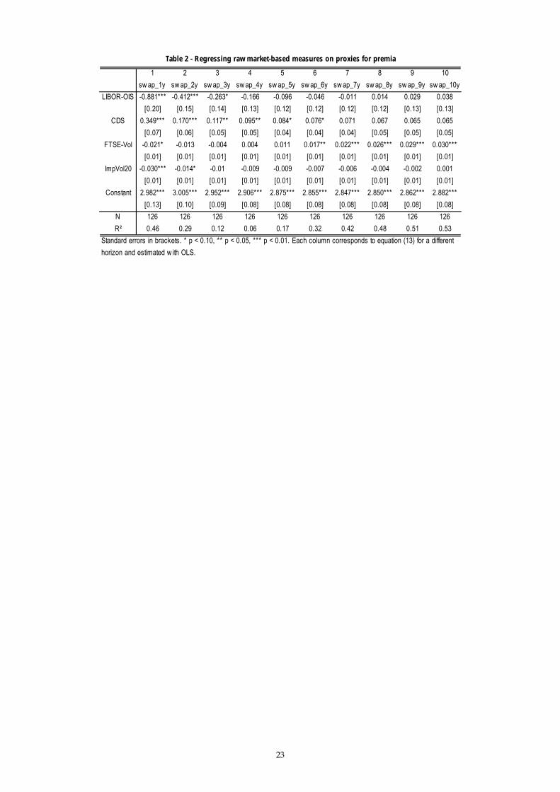
23

1 2 3 4 5 6 7 8 9 10

sw ap_1y sw ap_2y sw ap_3y sw ap_4y sw ap_5y sw ap_6y sw ap_7y sw ap_8y sw ap_9y sw ap_10y

LIBOR-OIS -0.881*** -0.412*** -0.263* -0.166 -0.096 -0.046 -0.011 0.014 0.029 0.038

[0.20] [0.15] [0.14] [0.13] [0.12] [0.12] [0.12] [0.12] [0.13] [0.13]

CDS 0.349*** 0.170*** 0.117** 0.095** 0.084* 0.076* 0.071 0.067 0.065 0.065

[0.07] [0.06] [0.05] [0.05] [0.04] [0.04] [0.04] [0.05] [0.05] [0.05]

FTSE-Vol -0.021* -0.013 -0.004 0.004 0.011 0.017** 0.022*** 0.026*** 0.029*** 0.030***

[0.01] [0.01] [0.01] [0.01] [0.01] [0.01] [0.01] [0.01] [0.01] [0.01]

ImpVol20 -0.030*** -0.014* -0.01 -0.009 -0.009 -0.007 -0.006 -0.004 -0.002 0.001

[0.01] [0.01] [0.01] [0.01] [0.01] [0.01] [0.01] [0.01] [0.01] [0.01]

Constant 2.982*** 3.005*** 2.952*** 2.906*** 2.875*** 2.855*** 2.847*** 2.850*** 2.862*** 2.882***

[0.13] [0.10] [0.09] [0.08] [0.08] [0.08] [0.08] [0.08] [0.08] [0.08]

N 126 126 126 126 126 126 126 126 126 126

R² 0.46 0.29 0.12 0.06 0.17 0.32 0.42 0.48 0.51 0.53

Table 2 - Regressing raw market-based measures on proxies for premia

Standard errors in brackets. * p < 0.10, ** p < 0.05, *** p < 0.01. Each column corresponds to equation (13) for a different

horizon and estimated w ith OLS.

24

1 2 3 4 5 6 7

Bankrate BoE_cpi_4 BoE_cpi_8 BoE_cpi_12 BoE_gdp_4 BoE_gdp_8 BoE_gdp_12

L.ΔBankrate 0.668*** . . . . . .

[0.17]

L.BoE_cpi_h . 0.484** 0.253 -0.014 . . .

[0.20] [0.18] [0.17]

L.BoE_gdp_h . . . . 0.077 0.194 0.346**

[0.27] [0.18] [0.15]

Bankrate . 0.613 0.263 0.209 -0.951*** -0.559** -0.110

[0.40] [0.20] [0.13] [0.28] [0.23] [0.16]

PCA_BoE_cpi 0.043** . . . 0.053 -0.058 -0.039

[0.02] [0.05] [0.05] [0.03]

PCA_BoE_gdp -0.132*** 0.120 -0.008 0.037 . . .

[0.03] [0.12] [0.06] [0.04]

PCA_BoE_mc 0.420*** -0.980** -0.092 -0.059 1.090*** 0.629** 0.219

[0.07] [0.45] [0.22] [0.15] [0.30] [0.25] [0.17]

ZLB dummy -1.300*** 0.347 0.957*** 0.518** 0.126 -0.69 -0.051

[0.22] [0.66] [0.33] [0.22] [0.59] [0.46] [0.30]

L.PCA_PF_cpi 0.014 0.084* 0.013 -0.004 -0.045 -0.038 -0.01

[0.01] [0.05] [0.02] [0.02] [0.04] [0.03] [0.02]

L.PCA_PF_gdp -0.063* 0.144 0.041 0.047 -0.039 -0.043 -0.061

[0.04] [0.13] [0.07] [0.04] [0.13] [0.09] [0.06]

L.PCA_PF_ir3m -0.063*** 0.180 -0.035 -0.025 -0.175** -0.092 -0.016

[0.02] [0.12] [0.06] [0.04] [0.08] [0.07] [0.05]

Constant 2.622*** 1.048 0.432 1.383** 3.909*** 3.195*** 1.447**

[0.22] [1.13] [0.60] [0.50] [1.10] [0.89] [0.66]

Controls: Zt-1

Yes Yes Yes Yes Yes Yes Yes

N 125 42 42 42 42 42 42

R² 0.99 0.68 0.83 0.82 0.90 0.78 0.82

Mean SD Min Max AR(1) AR(3) SF-test pv al.

Bankrate 0.00 0.21 -0.72 0.63 0.44*** 0.16* 0.11

BoE_cpi_4 0.00 0.19 -0.88 0.63 0.00 -0.08 0.00

BoE_cpi_8 0.00 0.09 -0.37 0.45 0.00 0.06 0.00

BoE_cpi_12 0.00 0.06 -0.19 0.26 0.00 0.07 0.00

BoE_gdp_4 0.00 0.15 -0.45 0.69 0.00 0.07 0.00

BoE_gdp_8 0.00 0.12 -0.55 0.48 0.00 -0.12 0.00BoE_gdp_12 0.00 0.08 -0.34 0.25 0.00 -0.06 0.00

Bankrate BoE_cpi_4 BoE_cpi_8 BoE_cpi_12 BoE_gdp_4 BoE_gdp_8 BoE_gdp_12

Bankrate 1

BoE_cpi_4 -0.10 1

BoE_cpi_8 -0.11 0.55 1

BoE_cpi_12 -0.05 0.14 0.76 1

BoE_gdp_4 0.17 0.01 0.10 0.12 1

BoE_gdp_8 0.16 -0.14 -0.04 0.02 0.55 1

BoE_gdp_12 0.08 -0.21 0.03 0.03 0.21 0.59 1

VAR(3) - F-stat 0.31 1.09 1.29 0.98 0.89 0.95 0.92

VAR(3) - p -v alue 0.99 0.37 0.22 0.48 0.58 0.52 0.54

VAR(6) - F-stat 0.49 0.79 1.16 1.09 1.30 0.69 0.99

VAR(6) - p-v alue 0.99 0.77 0.30 0.37 0.17 0.88 0.50

Table 3 - Extracting Exogenous Shocks

Standard errors in brackets. * p < 0.10, ** p < 0.05, *** p < 0.01. L is the lag operator. Each column corresponds to the

OLS estimation of equation (14). The Z v ector of controls includes CPI, Industrial production, Oil prices, Sterling

effectiv e ex change rate, Net lending, Housing prices, the FTSE index and a dummy for Forw ard Guidance. The SF-

test is the Shapiro-Francia W' test for normal data.

Predictability of exogenous shock series

Correlation of exogenous shock series

Properties of exogenous shock series

25

PF_1y PF_2y PF_3y PF_4y PF_5y PF_6y PF_7y PF_8y PF_9y PF_10yBankrate -0.179 -0.187** -0.177*** -0.162*** -0.143*** -0.125*** -0.106** -0.088* -0.073 -0.061

[0.12] [0.08] [0.07] [0.06] [0.05] [0.05] [0.05] [0.05] [0.05] [0.05]BoE_cpi_4 0.224* 0.169* 0.149** 0.130** 0.111* 0.097* 0.089* 0.085 0.081 0.076

[0.13] [0.09] [0.07] [0.06] [0.06] [0.05] [0.05] [0.05] [0.05] [0.06]BoE_gdp_4 0.150 0.195* 0.194** 0.160* 0.113 0.067 0.025 -0.014 -0.049 -0.079

[0.17] [0.12] [0.09] [0.08] [0.07] [0.07] [0.07] [0.07] [0.07] [0.07]Lag dep v ar 0.666*** 0.733*** 0.776*** 0.796*** 0.804*** 0.803*** 0.796*** 0.784*** 0.771*** 0.758***

[0.07] [0.07] [0.06] [0.06] [0.05] [0.05] [0.05] [0.05] [0.05] [0.05]Constant 0.916*** 0.713*** 0.593*** 0.545*** 0.534*** 0.547*** 0.579*** 0.623*** 0.671*** 0.718***

[0.24] [0.21] [0.18] [0.16] [0.15] [0.14] [0.14] [0.14] [0.15] [0.15]Controls: X

t & Z

tYes Yes Yes Yes Yes Yes Yes Yes Yes Yes

N 125 125 125 125 125 125 125 125 125 125R² 0.63 0.68 0.73 0.77 0.80 0.82 0.84 0.84 0.83 0.82

Bankrate 0.02 0.05 0.06 0.07 0.07 0.06 0.05 0.03 0.02 0.01BoE_cpi_4 0.03 0.03 0.04 0.04 0.03 0.03 0.02 0.02 0.02 0.02BoE_gdp_4 0.01 0.03 0.04 0.04 0.02 0.01 0.00 0.00 0.01 0.01

BoE_cpi_8 0.261 0.254 0.246 0.236* 0.223* 0.210* 0.200* 0.194* 0.192* 0.192[0.28] [0.19] [0.15] [0.13] [0.12] [0.11] [0.11] [0.11] [0.11] [0.12]

BoE_gdp_8 0.303 0.287** 0.265** 0.233** 0.194** 0.154* 0.115 0.078 0.043 0.013[0.20] [0.14] [0.11] [0.10] [0.09] [0.08] [0.08] [0.08] [0.08] [0.09]

R² 0.62 0.69 0.74 0.78 0.81 0.83 0.84 0.84 0.83 0.82

BoE_cpi_12 -0.108 -0.093 -0.078 -0.046 -0.009 0.029 0.072 0.12 0.171 0.222[0.49] [0.32] [0.27] [0.23] [0.20] [0.19] [0.19] [0.19] [0.20] [0.21]

BoE_gdp_12 0.133 0.154 0.189 0.213 0.230* 0.239* 0.242* 0.239* 0.231* 0.221[0.33] [0.22] [0.18] [0.15] [0.14] [0.13] [0.12] [0.13] [0.13] [0.14]

R² 0.60 0.68 0.72 0.76 0.79 0.81 0.82 0.82 0.81 0.80

Table 4 - Benchmark estimates and other horizons

Standard errors in brackets. * p < 0.10, ** p < 0.05, *** p < 0.01. Each column corresponds to the OLS estimation of

equation (11) for a giv en horizon of priv ate inflation ex pectations. The tw o low er panels show s the parameters for BoE

projections only , but estimated w ith the model described by equation (11). Xt includes the change betw een t-1 and t in

priv ate output forecasts and in priv ate 3-month interest rate forecasts, and a new s v ariable capturing the information flow

betw een t-1 and t of macro data releases related to inflation. Zt includes CPI, Industrial production, Oil prices, Sterling

effectiv e ex change rate, Net lending, Housing prices, the FTSE index and a dummy for Forw ard Guidance.

4-quarter-ahead BoE projections

8-quarter-ahead BoE projections

12-quarter-ahead BoE projections

Partial R² - Variance decomposition

26

PF_1y PF_2y PF_3y PF_4y PF_5y PF_6y PF_7y PF_8y PF_9y PF_10y

Bankrate*Output Gap 0.235*** 0.165*** 0.107*** 0.079*** 0.061*** 0.047** 0.033* 0.022 0.013 0.009

[0.04] [0.03] [0.03] [0.02] [0.02] [0.02] [0.02] [0.02] [0.02] [0.02]

Bankrate -0.02 -0.085 -0.106* -0.109* -0.105** -0.098** -0.089* -0.078 -0.068 -0.058

[0.11] [0.07] [0.06] [0.06] [0.05] [0.05] [0.05] [0.05] [0.05] [0.05]

BoE_cpi_4 0.221* 0.188** 0.165** 0.137** 0.114** 0.098* 0.090* 0.087 0.084 0.081

[0.12] [0.08] [0.07] [0.06] [0.06] [0.05] [0.05] [0.05] [0.06] [0.06]

BoE_gdp_4 0.137 0.178* 0.171* 0.137* 0.093 0.052 0.015 -0.019 -0.05 -0.079

[0.15] [0.10] [0.09] [0.08] [0.07] [0.07] [0.07] [0.07] [0.07] [0.07]

Lag dep v ar 0.790*** 0.853*** 0.850*** 0.844*** 0.837*** 0.823*** 0.804*** 0.783*** 0.765*** 0.750***

[0.07] [0.06] [0.06] [0.06] [0.05] [0.05] [0.05] [0.05] [0.05] [0.05]

Constant 0.588** 0.393** 0.400** 0.418*** 0.445*** 0.491*** 0.553*** 0.620*** 0.681*** 0.733***

[0.23] [0.19] [0.18] [0.16] [0.15] [0.14] [0.14] [0.14] [0.15] [0.16]

Controls: Xt & Z

tYes Yes Yes Yes Yes Yes Yes Yes Yes Yes

N 125 125 125 125 125 125 125 125 125 125

R² 0.71 0.75 0.77 0.79 0.815 0.83 0.84 0.84 0.83 0.82

Bankrate coefficient w ith:

Positiv e OG 0.423*** 0.226** 0.10 0.04 0.01 -0.01 -0.03 -0.04 -0.04 -0.04

[0.15] [0.10] [0.09] [0.08] [0.07] [0.07] [0.07] [0.07] [0.07] [0.07]

Negativ e OG -0.463*** -0.395*** -0.309*** -0.258*** -0.220*** -0.186*** -0.151*** -0.119** -0.093* -0.075

[0.12] [0.08] [0.07] [0.06] [0.06] [0.05] [0.05] [0.05] [0.05] [0.06]

PF_1y PF_2y PF_3y PF_4y PF_5y PF_6y PF_7y PF_8y PF_9y PF_10y

BoE_cpi*Output Gap -0.087 -0.082* -0.070* -0.056* -0.044 -0.032 -0.022 -0.013 -0.005 0.003

[0.06] [0.04] [0.04] [0.03] [0.03] [0.03] [0.03] [0.03] [0.03] [0.03]

Bankrate -0.171 -0.189** -0.181*** -0.166*** -0.147*** -0.128*** -0.109** -0.091* -0.076 -0.064

[0.11] [0.08] [0.07] [0.06] [0.05] [0.05] [0.05] [0.05] [0.05] [0.05]

BoE_cpi_4 0.172 0.127 0.118 0.106 0.094 0.086 0.083 0.083 0.083 0.081

[0.13] [0.09] [0.08] [0.07] [0.06] [0.05] [0.05] [0.05] [0.06] [0.06]

BoE_gdp_4 0.061 0.119 0.131 0.109 0.075 0.039 0.006 -0.024 -0.051 -0.074

[0.17] [0.12] [0.10] [0.09] [0.08] [0.07] [0.07] [0.07] [0.07] [0.08]

Lag dep v ar 0.659*** 0.737*** 0.783*** 0.801*** 0.805*** 0.800*** 0.790*** 0.776*** 0.762*** 0.750***

[0.07] [0.07] [0.06] [0.06] [0.05] [0.05] [0.05] [0.05] [0.05] [0.05]

Constant 0.979*** 0.733*** 0.596*** 0.547*** 0.541*** 0.560*** 0.597*** 0.643*** 0.690*** 0.733***

[0.24] [0.20] [0.18] [0.16] [0.15] [0.14] [0.14] [0.14] [0.15] [0.16]

Controls: Xt & Z

tYes Yes Yes Yes Yes Yes Yes Yes Yes Yes

N 125 125 125 125 125 125 125 125 125 125

R² 0.64 0.70 0.74 0.77 0.805 0.83 0.84 0.84 0.83 0.82

BoE_cpi coefficient w ith:

Positiv e OG 0.009 -0.029 -0.014 0.000 0.012 0.025 0.040 0.058 0.074 0.087

[0.19] [0.13] [0.11] [0.09] [0.09] [0.08] [0.08] [0.08] [0.08] [0.08]

Negativ e OG 0.335** 0.282*** 0.250*** 0.213*** 0.176** 0.147** 0.125* 0.107 0.091 0.075

[0.16] [0.11] [0.09] [0.08] [0.07] [0.07] [0.07] [0.07] [0.07] [0.07]

Table 5 - State-dependence of monetary and projection shocks

Bankrate * Output Gap

Standard errors in brackets. * p < 0.10, ** p < 0.05, *** p < 0.01. Each column corresponds to the OLS estimation of equation (11)

for different horizons of priv ate inflation ex pectations. Xt includes the change betw een t-1 and t in priv ate output forecasts and in

priv ate 3-month interest rate forecasts, and a new s v ariable capturing the information flow betw een t-1 and t of macro data releases

related to inflation. Zt includes CPI, Industrial production, Oil prices, Sterling effectiv e ex change rate, Net lending, Housing prices, the

FTSE index and a dummy for Forw ard Guidance.

BoE_cpi * Output Gap

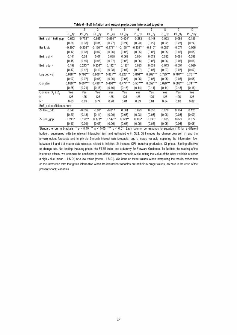
27

1 2 3 4 5 6 7 8 9 10PF_1y PF_2y PF_3y PF_4y PF_5y PF_6y PF_7y PF_8y PF_9y PF_10y

BoE_cpi * BoE_gdp -0.693 -0.772** -0.695** -0.564** -0.424* -0.283 -0.148 -0.023 0.089 0.183[0.56] [0.38] [0.31] [0.27] [0.24] [0.23] [0.22] [0.22] [0.23] [0.24]

Bankrate -0.200* -0.209** -0.196*** -0.178*** -0.155*** -0.133*** -0.110** -0.089* -0.071 -0.056[0.12] [0.08] [0.07] [0.06] [0.05] [0.05] [0.05] [0.05] [0.05] [0.05]

BoE_cpi_4 0.141 0.08 0.07 0.065 0.062 0.064 0.072 0.082 0.091 0.099[0.15] [0.10] [0.08] [0.07] [0.06] [0.06] [0.06] [0.06] [0.06] [0.06]

BoE_gdp_4 0.198 0.243** 0.234** 0.192** 0.137* 0.083 0.033 -0.013 -0.054 -0.089[0.17] [0.12] [0.10] [0.08] [0.07] [0.07] [0.07] [0.07] [0.07] [0.07]

Lag dep v ar 0.688*** 0.766*** 0.806*** 0.821*** 0.823*** 0.816*** 0.802*** 0.785*** 0.767*** 0.751***[0.07] [0.07] [0.06] [0.06] [0.05] [0.05] [0.05] [0.05] [0.05] [0.05]

Constant 0.839*** 0.607*** 0.496*** 0.466*** 0.474*** 0.507*** 0.559*** 0.620*** 0.683*** 0.741***[0.25] [0.21] [0.18] [0.16] [0.15] [0.14] [0.14] [0.14] [0.15] [0.16]

Controls: Xt & Z

tYes Yes Yes Yes Yes Yes Yes Yes Yes Yes

N 125 125 125 125 125 125 125 125 125 125R² 0.63 0.69 0.74 0.78 0.81 0.83 0.84 0.84 0.83 0.82BoE_cpi coefficient w hen:Δ+ BoE_gdp 0.040 -0.032 -0.031 -0.017 0.001 0.023 0.050 0.078 0.104 0.125

[0.20] [0.13] [0.11] [0.09] [0.08] [0.08] [0.08] [0.08] [0.08] [0.09]Δ- BoE_gdp 0.241* 0.192** 0.171** 0.147** 0.123** 0.105* 0.093* 0.085 0.079 0.072

[0.13] [0.09] [0.07] [0.06] [0.06] [0.05] [0.05] [0.05] [0.06] [0.06]

Table 6 - BoE inflation and output projections interacted together

Standard errors in brackets. * p < 0.10, ** p < 0.05, *** p < 0.01. Each column corresponds to equation (11) for a different

horizon, augmented w ith the relev ant interaction term and estimated w ith OLS. Xt includes the change betw een t-1 and t in

priv ate output forecasts and in priv ate 3-month interest rate forecasts, and a new s v ariable capturing the information flow

betw een t-1 and t of macro data releases related to inflation. Zt includes CPI, Industrial production, Oil prices, Sterling effectiv e

ex change rate, Net lending, Housing prices, the FTSE index and a dummy for Forw ard Guidance. To facilitate the reading of the

interacted effects, w e compute the coefficient of one of the interacted v ariable w hile setting the v alue of the other v ariable at either

a high v alue (mean + 1 S.D.) or a low v alue (mean - 1 S.D.). We focus on these v alues w hen interpreting the results rather than

on the interaction term that giv es information w hen the interaction v ariables are at their av erage v alues, so zero in the case of the

present shock v ariables.

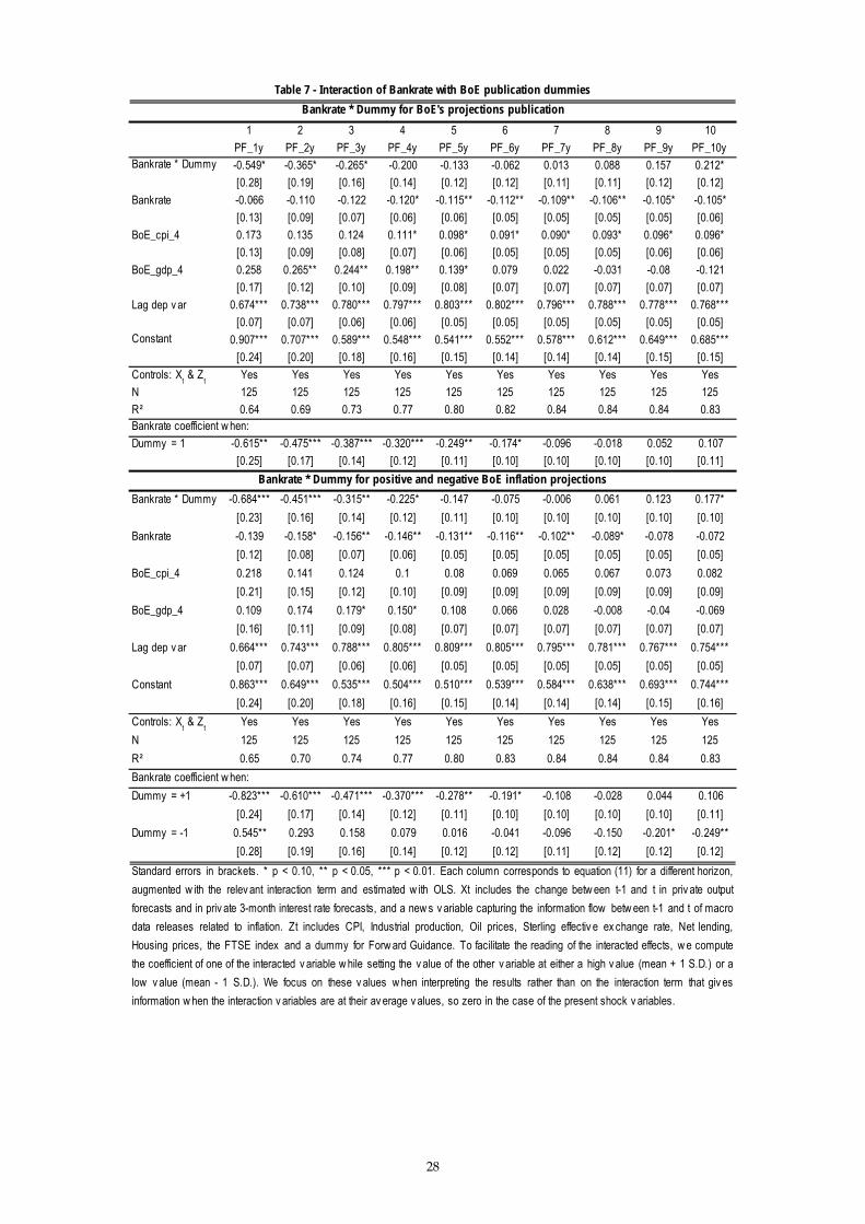
28

1 2 3 4 5 6 7 8 9 10

PF_1y PF_2y PF_3y PF_4y PF_5y PF_6y PF_7y PF_8y PF_9y PF_10yBankrate * Dummy -0.549* -0.365* -0.265* -0.200 -0.133 -0.062 0.013 0.088 0.157 0.212*

[0.28] [0.19] [0.16] [0.14] [0.12] [0.12] [0.11] [0.11] [0.12] [0.12]

Bankrate -0.066 -0.110 -0.122 -0.120* -0.115** -0.112** -0.109** -0.106** -0.105* -0.105*

[0.13] [0.09] [0.07] [0.06] [0.06] [0.05] [0.05] [0.05] [0.05] [0.06]

BoE_cpi_4 0.173 0.135 0.124 0.111* 0.098* 0.091* 0.090* 0.093* 0.096* 0.096*

[0.13] [0.09] [0.08] [0.07] [0.06] [0.05] [0.05] [0.05] [0.06] [0.06]

BoE_gdp_4 0.258 0.265** 0.244** 0.198** 0.139* 0.079 0.022 -0.031 -0.08 -0.121

[0.17] [0.12] [0.10] [0.09] [0.08] [0.07] [0.07] [0.07] [0.07] [0.07]

Lag dep v ar 0.674*** 0.738*** 0.780*** 0.797*** 0.803*** 0.802*** 0.796*** 0.788*** 0.778*** 0.768***

[0.07] [0.07] [0.06] [0.06] [0.05] [0.05] [0.05] [0.05] [0.05] [0.05]Constant 0.907*** 0.707*** 0.589*** 0.548*** 0.541*** 0.552*** 0.578*** 0.612*** 0.649*** 0.685***

[0.24] [0.20] [0.18] [0.16] [0.15] [0.14] [0.14] [0.14] [0.15] [0.15]

Controls: Xt & Z

tYes Yes Yes Yes Yes Yes Yes Yes Yes Yes

N 125 125 125 125 125 125 125 125 125 125

R² 0.64 0.69 0.73 0.77 0.80 0.82 0.84 0.84 0.84 0.83Bankrate coefficient w hen:

Dummy = 1 -0.615** -0.475*** -0.387*** -0.320*** -0.249** -0.174* -0.096 -0.018 0.052 0.107

[0.25] [0.17] [0.14] [0.12] [0.11] [0.10] [0.10] [0.10] [0.10] [0.11]

Bankrate * Dummy -0.684*** -0.451*** -0.315** -0.225* -0.147 -0.075 -0.006 0.061 0.123 0.177*

[0.23] [0.16] [0.14] [0.12] [0.11] [0.10] [0.10] [0.10] [0.10] [0.10]

Bankrate -0.139 -0.158* -0.156** -0.146** -0.131** -0.116** -0.102** -0.089* -0.078 -0.072

[0.12] [0.08] [0.07] [0.06] [0.05] [0.05] [0.05] [0.05] [0.05] [0.05]

BoE_cpi_4 0.218 0.141 0.124 0.1 0.08 0.069 0.065 0.067 0.073 0.082

[0.21] [0.15] [0.12] [0.10] [0.09] [0.09] [0.09] [0.09] [0.09] [0.09]

BoE_gdp_4 0.109 0.174 0.179* 0.150* 0.108 0.066 0.028 -0.008 -0.04 -0.069

[0.16] [0.11] [0.09] [0.08] [0.07] [0.07] [0.07] [0.07] [0.07] [0.07]

Lag dep v ar 0.664*** 0.743*** 0.788*** 0.805*** 0.809*** 0.805*** 0.795*** 0.781*** 0.767*** 0.754***

[0.07] [0.07] [0.06] [0.06] [0.05] [0.05] [0.05] [0.05] [0.05] [0.05]

Constant 0.863*** 0.649*** 0.535*** 0.504*** 0.510*** 0.539*** 0.584*** 0.638*** 0.693*** 0.744***

[0.24] [0.20] [0.18] [0.16] [0.15] [0.14] [0.14] [0.14] [0.15] [0.16]

Controls: Xt & Z

tYes Yes Yes Yes Yes Yes Yes Yes Yes Yes

N 125 125 125 125 125 125 125 125 125 125

R² 0.65 0.70 0.74 0.77 0.80 0.83 0.84 0.84 0.84 0.83

Bankrate coefficient w hen:

Dummy = +1 -0.823*** -0.610*** -0.471*** -0.370*** -0.278** -0.191* -0.108 -0.028 0.044 0.106

[0.24] [0.17] [0.14] [0.12] [0.11] [0.10] [0.10] [0.10] [0.10] [0.11]

Dummy = -1 0.545** 0.293 0.158 0.079 0.016 -0.041 -0.096 -0.150 -0.201* -0.249**

[0.28] [0.19] [0.16] [0.14] [0.12] [0.12] [0.11] [0.12] [0.12] [0.12]

Bankrate * Dummy for BoE's projections publication

Bankrate * Dummy for positive and negative BoE inflation projections

Table 7 - Interaction of Bankrate with BoE publication dummies

Standard errors in brackets. * p < 0.10, ** p < 0.05, *** p < 0.01. Each column corresponds to equation (11) for a different horizon,

augmented w ith the relev ant interaction term and estimated w ith OLS. Xt includes the change betw een t-1 and t in priv ate output

forecasts and in priv ate 3-month interest rate forecasts, and a new s v ariable capturing the information flow betw een t-1 and t of macro

data releases related to inflation. Zt includes CPI, Industrial production, Oil prices, Sterling effectiv e ex change rate, Net lending,

Housing prices, the FTSE index and a dummy for Forw ard Guidance. To facilitate the reading of the interacted effects, w e compute

the coefficient of one of the interacted v ariable w hile setting the v alue of the other v ariable at either a high v alue (mean + 1 S.D.) or a

low v alue (mean - 1 S.D.). We focus on these v alues w hen interpreting the results rather than on the interaction term that giv es

information w hen the interaction v ariables are at their av erage v alues, so zero in the case of the present shock v ariables.

29

1 2 3 4 5 6 7 8 9 10

PF_1y PF_2y PF_3y PF_4y PF_5y PF_6y PF_7y PF_8y PF_9y PF_10yBankrate * BoE_cpi -1.530* -1.258** -0.967* -0.668 -0.375 -0.11 0.125 0.334 0.519 0.680*

[0.87] [0.60] [0.50] [0.43] [0.39] [0.36] [0.35] [0.36] [0.36] [0.38]

Bankrate -0.16 -0.174** -0.168** -0.155*** -0.139*** -0.123** -0.107** -0.092* -0.079 -0.069

[0.11] [0.08] [0.07] [0.06] [0.05] [0.05] [0.05] [0.05] [0.05] [0.05]

BoE_cpi_4 0.149 0.108 0.104 0.099 0.093 0.092 0.095* 0.101* 0.107* 0.111*

[0.14] [0.09] [0.08] [0.07] [0.06] [0.06] [0.06] [0.06] [0.06] [0.06]

BoE_gdp_4 0.103 0.161 0.167* 0.141* 0.102 0.064 0.028 -0.004 -0.033 -0.058

[0.17] [0.11] [0.09] [0.08] [0.07] [0.07] [0.07] [0.07] [0.07] [0.07]

Lag dep v ar 0.661*** 0.741*** 0.789*** 0.807*** 0.811*** 0.805*** 0.794*** 0.779*** 0.763*** 0.749***

[0.07] [0.07] [0.06] [0.06] [0.05] [0.05] [0.05] [0.05] [0.05] [0.05]Constant 0.929*** 0.691*** 0.557*** 0.515*** 0.516*** 0.542*** 0.585*** 0.638*** 0.692*** 0.743***

[0.24] [0.20] [0.18] [0.16] [0.15] [0.14] [0.14] [0.14] [0.15] [0.15]

Controls: Xt & Z

tYes Yes Yes Yes Yes Yes Yes Yes Yes Yes

N 125 125 125 125 125 125 125 125 125 125

R² 0.64 0.69 0.73 0.77 0.80 0.82 0.84 0.84 0.84 0.83Bankrate coefficient w hen:

Δ+ BoE_cpi -0.444** -0.408*** -0.347*** -0.279*** -0.209** -0.144* -0.084 -0.030 0.017 0.057

[0.19] [0.13] [0.11] [0.09] [0.08] [0.08] [0.08] [0.08] [0.08] [0.08]

Δ- BoE_cpi 0.124 0.059 0.012 -0.031 -0.069 -0.103 -0.131 -0.154* -0.176** -0.195**

[0.21] [0.14] [0.12] [0.10] [0.09] [0.09] [0.08] [0.08] [0.09] [0.09]

Bankrate * BoE_gdp -0.503 -0.103 -0.01 0.009 0.034 0.051 0.075 0.121 0.189 0.274

[1.02] [0.71] [0.59] [0.51] [0.45] [0.42] [0.41] [0.41] [0.42] [0.44]

Bankrate -0.179 -0.187** -0.177*** -0.162*** -0.143*** -0.125*** -0.106** -0.089* -0.073 -0.062

[0.12] [0.08] [0.07] [0.06] [0.05] [0.05] [0.05] [0.05] [0.05] [0.05]

BoE_cpi_4 0.216 0.168* 0.149** 0.130** 0.112* 0.098* 0.090* 0.086 0.083 0.08

[0.13] [0.09] [0.08] [0.06] [0.06] [0.05] [0.05] [0.05] [0.06] [0.06]

BoE_gdp_4 0.132 0.192 0.193** 0.160* 0.114 0.069 0.027 -0.01 -0.042 -0.069

[0.17] [0.12] [0.10] [0.08] [0.07] [0.07] [0.07] [0.07] [0.07] [0.07]

Lag dep v ar 0.669*** 0.735*** 0.776*** 0.796*** 0.803*** 0.802*** 0.794*** 0.782*** 0.768*** 0.754***

[0.07] [0.07] [0.06] [0.06] [0.05] [0.05] [0.05] [0.05] [0.05] [0.05]

Constant 0.921*** 0.712*** 0.593*** 0.546*** 0.535*** 0.549*** 0.581*** 0.625*** 0.673*** 0.719***

[0.24] [0.21] [0.18] [0.16] [0.15] [0.14] [0.14] [0.14] [0.15] [0.16]

Controls: Xt & Z

tYes Yes Yes Yes Yes Yes Yes Yes Yes Yes

N 125 125 125 125 125 125 125 125 125 125

R² 0.63 0.68 0.73 0.77 0.80 0.82 0.84 0.84 0.83 0.82

Bankrate coefficient w hen:

Δ+ BoE_gdp -0.252 -0.202 -0.179* -0.161* -0.138* -0.117 -0.095 -0.071 -0.046 -0.022

[0.19] [0.13] [0.11] [0.09] [0.08] [0.08] [0.07] [0.07] [0.08] [0.08]

Δ- BoE_gdp -0.106 -0.173 -0.176 -0.163* -0.148* -0.132* -0.117 -0.106 -0.101 -0.101

[0.19] [0.13] [0.11] [0.09] [0.08] [0.08] [0.08] [0.08] [0.08] [0.08]

Table 8 - Interaction of Bankrate with BoE inflation or output projections

Bankrate * BoE_cpi

Bankrate * BoE_gdp

Standard errors in brackets. * p < 0.10, ** p < 0.05, *** p < 0.01. Each column corresponds to equation (11) for a different horizon,

augmented w ith the relev ant interaction term and estimated w ith OLS. Xt includes the change betw een t-1 and t in priv ate output

forecasts and in priv ate 3-month interest rate forecasts, and a new s v ariable capturing the information flow betw een t-1 and t of

macro data releases related to inflation. Zt includes CPI, Industrial production, Oil prices, Sterling effectiv e ex change rate, Net

lending, Housing prices, the FTSE index and a dummy for Forw ard Guidance. To facilitate the reading of the interacted effects, w e

compute the coefficient of one of the interacted v ariable w hile setting the v alue of the other v ariable at either a high v alue (mean + 1

S.D.) or a low v alue (mean - 1 S.D.). We focus on these v alues w hen interpreting the results rather than on the interaction term that

giv es information w hen the interaction v ariables are at their av erage v alues, so zero in the case of the present shock v ariables.

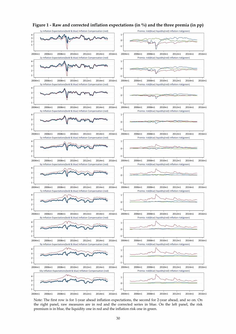
30

Figure 1 - Raw and corrected inflation expectations (in %) and the three premia (in pp)

Note: The first row is for 1-year ahead inflation expectations, the second for 2-year ahead, and so on. On the right panel, raw measures are in red and the corrected series in blue. On the left panel, the risk premium is in blue, the liquidity one in red and the inflation risk one in green.

1

2

3

4

2004m1 2006m1 2008m1 2010m1 2012m1 2014m1 2016m1

1y Inflation Expectations(bold & blue) Inflation Compensation (red)

1

2

3

4

2004m1 2006m1 2008m1 2010m1 2012m1 2014m1 2016m1

2y Inflation Expectations(bold & blue) Inflation Compensation (red)

1

2

3

4

2004m1 2006m1 2008m1 2010m1 2012m1 2014m1 2016m1

3y Inflation Expectations(bold & blue) Inflation Compensation (red)

1

2

3

4

2004m1 2006m1 2008m1 2010m1 2012m1 2014m1 2016m1

4y Inflation Expectations(bold & blue) Inflation Compensation (red)

1

2

3

4

2004m1 2006m1 2008m1 2010m1 2012m1 2014m1 2016m1

5y Inflation Expectations(bold & blue) Inflation Compensation (red)

1

2

3

4

2004m1 2006m1 2008m1 2010m1 2012m1 2014m1 2016m1

6y Inflation Expectations(bold & blue) Inflation Compensation (red)

1

2

3

4

2004m1 2006m1 2008m1 2010m1 2012m1 2014m1 2016m1

7y Inflation Expectations(bold & blue) Inflation Compensation (red)

1

2

3

4

2004m1 2006m1 2008m1 2010m1 2012m1 2014m1 2016m1

8y Inflation Expectations(bold & blue) Inflation Compensation (red)

1

2

3

4

2004m1 2006m1 2008m1 2010m1 2012m1 2014m1 2016m1

9y Inflation Expectations(bold & blue) Inflation Compensation (red)

1

2

3

4

2004m1 2006m1 2008m1 2010m1 2012m1 2014m1 2016m1

10y Inflation Expectations(bold & blue) Inflation Compensation (red)

‐1

0

1

2004m1 2006m1 2008m1 2010m1 2012m1 2014m1 2016m1

Premia: risk(blue) liquidity(red) inflation risk(green)

‐1

0

1

2004m1 2006m1 2008m1 2010m1 2012m1 2014m1 2016m1

Premia: risk(blue) liquidity(red) inflation risk(green)

‐1

0

1

2004m1 2006m1 2008m1 2010m1 2012m1 2014m1 2016m1

Premia: risk(blue) liquidity(red) inflation risk(green)

‐1

0

1

2004m1 2006m1 2008m1 2010m1 2012m1 2014m1 2016m1

Premia: risk(blue) liquidity(red) inflation risk(green)

‐1

0

1

2004m1 2006m1 2008m1 2010m1 2012m1 2014m1 2016m1

Premia: risk(blue) liquidity(red) inflation risk(green)

‐1

0

1

2004m1 2006m1 2008m1 2010m1 2012m1 2014m1 2016m1

Premia: risk(blue) liquidity(red) inflation risk(green)

‐1

0

1

2004m1 2006m1 2008m1 2010m1 2012m1 2014m1 2016m1

Premia: risk(blue) liquidity(red) inflation risk(green)

‐1

0

1

2004m1 2006m1 2008m1 2010m1 2012m1 2014m1 2016m1

Premia: risk(blue) liquidity(red) inflation risk(green)

‐1

0

1

2004m1 2006m1 2008m1 2010m1 2012m1 2014m1 2016m1

Premia: risk(blue) liquidity(red) inflation risk(green)

‐1

0

1

2004m1 2006m1 2008m1 2010m1 2012m1 2014m1 2016m1

Premia: risk(blue) liquidity(red) inflation risk(green)

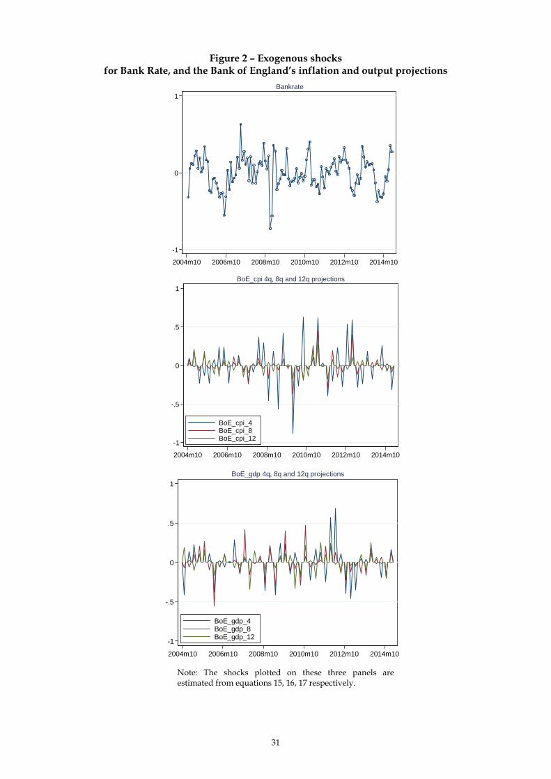
31

Figure 2 – Exogenous shocks for Bank Rate, and the Bank of England’s inflation and output projections

Note: The shocks plotted on these three panels are estimated from equations 15, 16, 17 respectively.

-1

0

1

2004m10 2006m10 2008m10 2010m10 2012m10 2014m10

Bankrate

-1

-.5

0

.5

1

2004m10 2006m10 2008m10 2010m10 2012m10 2014m10

BoE_cpi_4BoE_cpi_8BoE_cpi_12

BoE_cpi 4q, 8q and 12q projections

-1

-.5

0

.5

1

2004m10 2006m10 2008m10 2010m10 2012m10 2014m10

BoE_gdp_4BoE_gdp_8BoE_gdp_12

BoE_gdp 4q, 8q and 12q projections

32

Figure 3 – Effect of the Bank’s inflation projections interacted with Bank’s output projections

Note: Vertical bars indicate 1 S.E. confidence intervals. The red values correspond to the linear effect of the Bank’s inflation projections estimated in Table 4, while the black values correspond to the interaction effects estimated in Table 6.

Figure 4 – Effect of Bank Rate interacted with the Bank’s inflation projections

Note: Vertical bars indicate 1 S.E. confidence intervals. The red values correspond to the linear effect of Bank Rate estimated in Table 4, while the black values correspond to the interaction effects estimated in Table 8 upper panel.

33

APPENDIX

Variable Source Description

PF_hBloomberg and Bank of England

calculations

Inflation ex pectation measures deriv ed from inflation sw aps. Instantaneous forw ard inflation

rates for annual RPI inflation h y ears ahead. Monthly av erage of daily observ ations. Bankrate Bank of England Bank of England's policy interest rate.

BoE_cpi_h Bank of EnglandBank of England's modal projections for annual CPI inflation h quarters ahead, based on

market interest rate ex pectations.

BoE_gdp_h Bank of EnglandBank of England's modal projections for annual GDP grow th h quarters ahead, based on

market interest rate ex pectations.

PF_gdp_hConsensus Forecasts / Surv ey

of Ex ternal Forecasters

Consensus Forecasts' av erage projections for annual GDP grow th h quarters ahead, for h=1

to 6. Surv ey of Ex ternal Forecasters' av erage projections for annual GDP grow th h quarters

ahead, for h=8 and 12. Monthly constant interpolation from quarterly frequency .

ir3m_hBloomberg and Bank of England

calculations

3-Month market interest ex pectations deriv ed from nominal gov ernment bonds h y ears

ahead. Monthly av erage of daily observ ations.

irchange Authors' computationDummy that equals 1 w hen there is a change in Bankrate in a month in w hich the Inflation

Report is published.

mc_h Bank of England Market interest rate curv e used as conditioning path for BoE's macroeconomic projections.

PF-G_hBloomberg and Bank of England

calculations

Breakev en inflation ex pectation measures deriv ed from nominal and index -linked

gov ernment bonds.

Shadow rate Bank of England calculations Bankrate adjusted for internal estimates of the impact of QE.

CITI_1y Citigroup/YouGov Citigroup/YouGov measure of households' inflation ex pectations 1 y ear ahead.

SEF_2y Surv ey of Ex ternal ForecastersSurv ey of Ex ternal Forecasters' measure of annual CPI inflation ex pectations 2 y ears

ahead. Monthly constant interpolation from quarterly frequency .

SEF_3y Surv ey of Ex ternal ForecastersSurv ey of Ex ternal Forecasters' measure of annual CPI inflation ex pectations 3 y ears

ahead. Monthly constant interpolation from quarterly frequency .

CITI_5y 5 Citigroup/YouGov Citigroup/YouGov measure of households' inflation ex pectations 5-10 y ears ahead.

RPI surprises ONS and BloombergDifference betw een the outturn for annual RPI inflation in a giv en month and the market

median forecast 1 month before.

CPI ONS Annual % change in the Consumer Price Index .

Indpro ONS Annual real Industrial Production grow th seasonally adjusted.

Oil FRED Crude oil spot prices, Brent - Europe. Annual % change.

Sterling Bank of England Effectiv e ex change rate index , January 2005 = 100. Annual % change.

Netlending Bank of England12 month grow th rate of monetary financial institutions' sterling net lending to priv ate non-

financial corporations (ex cluding the effects of securitisations and loan transfers) (SA).

Housing Halifax and Nationw ideAv erage of (SA) Halifax and Nationw ide measures of av erage house prices. Annual %

change.

FTSE Bloomberg FTSE all-share index . Annual change.

FG Authors' computation Dummy that equals 1 during the period for w hich Forw ard Guidance on policy w as in place.

ZLB Authors' computation Dummy that equals 1 during the period Bankrate is at its effectiv e low er bound of 0.5%.

LIBOR-OIS FRED and Thomson DataStream3-Month London Interbank Offered Rate and 3-Month Ov ernight Index ed Sw ap rates.

Monthly av erage of daily observ ations.

CDSMarkit Group Limited and Bank of

England calculations

Unw eighted av erage of the fiv e-y ear CDS premia for the major UK lenders. Monthly

av erage of daily observ ations.

FTSE-Vol BloombergFTSE 100 Implied Volatility Index , 3 months constant maturity . Monthly av erage of daily

observ ations.

ImpVol20 Barclay s Liv eAt-the-money implied v olatility of 1 y ear LIBOR sw aptions, 20 y ears constant maturity .

Monthly av erage of daily observ ations.

Table A1 - Data description

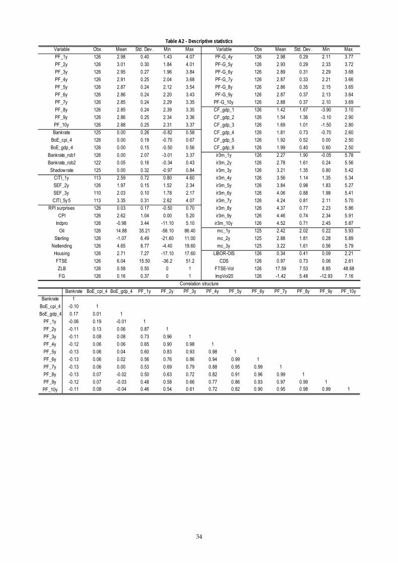
34

Obs Mean Std. Dev . Min Max Obs Mean Std. Dev . Min Max

126 2.98 0.40 1.43 4.07 126 2.98 0.29 2.11 3.77

126 3.01 0.30 1.84 4.01 126 2.93 0.29 2.33 3.72

126 2.95 0.27 1.96 3.84 126 2.89 0.31 2.29 3.68

126 2.91 0.25 2.04 3.68 126 2.87 0.33 2.21 3.66

126 2.87 0.24 2.12 3.54 126 2.86 0.35 2.15 3.65

126 2.86 0.24 2.20 3.43 126 2.87 0.37 2.13 3.64

126 2.85 0.24 2.29 3.35 126 2.88 0.37 2.10 3.69

126 2.85 0.24 2.39 3.35 126 1.42 1.67 -3.90 3.10

126 2.86 0.25 2.34 3.36 126 1.54 1.36 -3.10 2.90

126 2.88 0.25 2.31 3.37 126 1.69 1.01 -1.50 2.80

125 0.00 0.26 -0.82 0.58 126 1.81 0.73 -0.70 2.60

126 0.00 0.19 -0.70 0.67 126 1.92 0.52 0.00 2.50

126 0.00 0.15 -0.50 0.56 126 1.99 0.40 0.60 2.50

126 0.00 2.07 -3.01 3.37 126 2.27 1.90 -0.05 5.78

122 0.05 0.16 -0.34 0.43 126 2.78 1.61 0.24 5.56

125 0.00 0.32 -0.97 0.84 126 3.21 1.35 0.80 5.42

113 2.59 0.72 0.80 4.60 126 3.56 1.14 1.35 5.34

126 1.97 0.15 1.52 2.34 126 3.84 0.98 1.83 5.27

110 2.03 0.10 1.78 2.17 126 4.06 0.88 1.98 5.41

113 3.35 0.31 2.62 4.07 126 4.24 0.81 2.11 5.70

126 0.03 0.17 -0.50 0.70 126 4.37 0.77 2.23 5.86

126 2.62 1.04 0.00 5.20 126 4.46 0.74 2.34 5.91

126 -0.98 3.44 -11.10 5.10 126 4.52 0.71 2.45 5.87

126 14.88 35.21 -56.10 86.40 125 2.42 2.02 0.22 5.93

126 -1.07 6.49 -21.60 11.00 125 2.88 1.81 0.28 5.89

126 4.65 8.77 -4.40 19.60 125 3.22 1.61 0.56 5.79

126 2.71 7.27 -17.10 17.60 126 0.34 0.41 0.09 2.21

126 6.04 15.50 -36.2 51.2 126 0.97 0.73 0.06 2.61

126 0.58 0.50 0 1 126 17.59 7.53 8.85 48.68

126 0.16 0.37 0 1 126 -1.42 5.48 -12.93 7.16

Bankrate BoE_cpi_4 BoE_gdp_4 PF_1y PF_2y PF_3y PF_4y PF_5y PF_6y PF_7y PF_8y PF_9y PF_10y

Bankrate 1

BoE_cpi_4 -0.10 1

BoE_gdp_4 0.17 0.01 1

PF_1y -0.06 0.19 -0.01 1

PF_2y -0.11 0.13 0.06 0.87 1

PF_3y -0.11 0.08 0.08 0.73 0.96 1

PF_4y -0.12 0.06 0.06 0.65 0.90 0.98 1

PF_5y -0.13 0.06 0.04 0.60 0.83 0.93 0.98 1

PF_6y -0.13 0.06 0.02 0.56 0.76 0.86 0.94 0.99 1

PF_7y -0.13 0.06 0.00 0.53 0.69 0.79 0.88 0.95 0.99 1

PF_8y -0.13 0.07 -0.02 0.50 0.63 0.72 0.82 0.91 0.96 0.99 1

PF_9y -0.12 0.07 -0.03 0.48 0.58 0.66 0.77 0.86 0.93 0.97 0.99 1

PF_10y -0.11 0.08 -0.04 0.46 0.54 0.61 0.72 0.82 0.90 0.95 0.98 0.99 1

Table A2 - Descriptive statistics

FG

ZLB

FTSE

Housing

Netlending

Sterling

Oil

Indpro

CPI

RPI surprises

CITI_5y 5

SEF_3y

SEF_2y

CITI_1y

Shadow rate

Bankrate_rob2

Bankrate_rob1

BoE_gdp_4

BoE_cpi_4

Bankrate

PF_10y

PF_9y

PF_8y

PF_7y

PF_6y

Variable

PF_5y

PF_4y

PF_3y

PF_2y

PF_1y

LIBOR-OIS

mc_3y

Variable

CF_gdp_6

CF_gdp_5

CF_gdp_4

CF_gdp_3

CF_gdp_2

CF_gdp_1

PF-G_10y

PF-G_9y

PF-G_8y

PF-G_7y

PF-G_6y

PF-G_5y

PF-G_4y

Correlation structure

ir3m_2y

ir3m_1y

ir3m_7y

ir3m_6y

ir3m_5y

ir3m_4y

ir3m_3y

mc_2y

mc_1y

ir3m_10y

ir3m_9y

ir3m_8y

ImpVol20

FTSE-Vol

CDS

35

PF'_1y PF'_2y PF'_3y PF'_4y PF'_5y PF'_6y PF'_7y PF'_8y PF'_9y PF'_10y

Bankrate -0.142 -0.197* -0.211** -0.207** -0.190*** -0.168** -0.144** -0.120** -0.097* -0.077

[0.13] [0.11] [0.09] [0.08] [0.07] [0.06] [0.06] [0.06] [0.06] [0.06]

BoE_cpi_4 0.234 0.111 0.051 0.016 -0.009 -0.023 -0.029 -0.031 -0.031 -0.032

[0.15] [0.12] [0.10] [0.09] [0.08] [0.07] [0.07] [0.07] [0.07] [0.07]

BoE_gdp_4 0.107 0.155 0.156 0.118 0.07 0.024 -0.018 -0.055 -0.09 -0.12

[0.19] [0.15] [0.13] [0.12] [0.10] [0.09] [0.09] [0.08] [0.08] [0.08]

Lag dep v ar 0.627*** 0.578*** 0.588*** 0.630*** 0.671*** 0.704*** 0.729*** 0.744*** 0.750*** 0.749***

[0.08] [0.08] [0.08] [0.07] [0.07] [0.06] [0.06] [0.06] [0.06] [0.06]

Constant 1.119*** 1.170*** 1.095*** 0.979*** 0.881*** 0.808*** 0.762*** 0.740*** 0.740*** 0.757***

[0.27] [0.25] [0.23] [0.21] [0.19] [0.18] [0.17] [0.17] [0.17] [0.17]

Controls: Xt & Z

tYes Yes Yes Yes Yes Yes Yes Yes Yes Yes

N 125 125 125 125 125 125 125 125 125 125R² 0.56 0.54 0.57 0.62 0.67 0.71 0.75 0.77 0.78 0.79

PF-G_1y PF-G_2y PF-G_3y PF-G_4y PF-G_5y PF-G_6y PF-G_7y PF-G_8y PF-G_9y PF-G_10y

Bankrate . . . -0.123* -0.115* -0.110* -0.102* -0.091 -0.08 -0.072

[0.07] [0.06] [0.06] [0.06] [0.06] [0.07] [0.07]

BoE_cpi_4 . . . 0.132* 0.108 0.088 0.074 0.066 0.061 0.058

[0.08] [0.07] [0.07] [0.07] [0.07] [0.08] [0.08]

BoE_gdp_4 . . . 0.041 0.045 0.026 -0.012 -0.058 -0.106 -0.151

[0.09] [0.09] [0.08] [0.08] [0.09] [0.09] [0.10]

Lag dep v ar . . . 0.801*** 0.826*** 0.840*** 0.843*** 0.841*** 0.838*** 0.834***

[0.06] [0.06] [0.05] [0.05] [0.05] [0.05] [0.05]

Constant . . . 0.582*** 0.550*** 0.531*** 0.538*** 0.556*** 0.576*** 0.598***

[0.17] [0.16] [0.15] [0.14] [0.14] [0.15] [0.15]

Controls: Xt & Z

t. . . Yes Yes Yes Yes Yes Yes Yes

N . . . 125 125 125 125 125 125 125R² . . . 0.76 0.81 0.84 0.86 0.86 0.85 0.84

PF''_1y PF''_2y PF''_3y PF''_4y PF''_5y PF''_6y PF''_7y PF''_8y PF''_9y PF''_10y

Bankrate -0.244** -0.219** -0.184** -0.153** -0.121** -0.090** -0.06 -0.032 -0.008 0.013

[0.12] [0.09] [0.07] [0.06] [0.05] [0.04] [0.04] [0.03] [0.03] [0.04]

BoE_cpi_4 0.243* 0.191** 0.153* 0.120* 0.093* 0.074 0.062 0.053 0.046 0.039

[0.13] [0.10] [0.08] [0.06] [0.05] [0.05] [0.04] [0.04] [0.04] [0.04]

BoE_gdp_4 0.207 0.202 0.188* 0.154* 0.111 0.069 0.029 -0.009 -0.043 -0.072

[0.17] [0.13] [0.10] [0.09] [0.07] [0.06] [0.05] [0.05] [0.05] [0.05]

Lag dep v ar 0.736*** 0.739*** 0.765*** 0.795*** 0.825*** 0.849*** 0.866*** 0.878*** 0.886*** 0.893***

[0.07] [0.07] [0.06] [0.06] [0.05] [0.04] [0.04] [0.03] [0.03] [0.04]

Constant 0.745*** 0.705*** 0.635*** 0.562*** 0.488*** 0.428*** 0.386*** 0.359*** 0.340*** 0.326**

[0.22] [0.20] [0.19] [0.17] [0.15] [0.13] [0.12] [0.12] [0.12] [0.13]

Controls: Xt & Z

tYes Yes Yes Yes Yes Yes Yes Yes Yes Yes

N 125 125 125 125 125 125 125 125 125 125R² 0.79 0.73 0.71 0.76 0.85 0.91 0.94 0.95 0.96 0.96

Table A3 - Robustness checks on the left-hand side variable

Standard errors in brackets. * p < 0.10, ** p < 0.05, *** p < 0.01. Each column corresponds to equation (11) for a different

horizon and estimated w ith OLS. PF' is the sw ap measure of inflation ex pectations based on the last observ ation in each month

(rather than the av erage of observ ations). PF'' is the inflation compensation measure, so w ithout correction for the risk, liquidity

and inflation risk premia. Xt includes the change betw een t-1 and t in priv ate output forecasts and in priv ate 3-month interest rate

forecasts, and a new s v ariable capturing the information flow betw een t-1 and t of macro data releases related to inflation. Zt

includes CPI, Industrial production, Oil prices, Sterling effectiv e ex change rate, Net lending, Housing prices, the FTSE index and

a dummy for Forw ard Guidance.

Last observation

Gilts

Without correction for premia

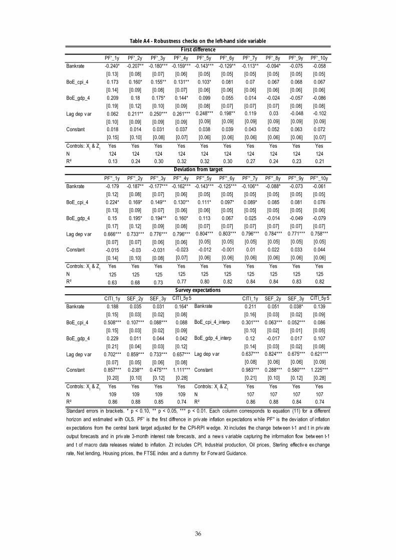
36

PF'_1y PF'_2y PF'_3y PF'_4y PF'_5y PF'_6y PF'_7y PF'_8y PF'_9y PF'_10y

Bankrate -0.240* -0.207** -0.180*** -0.159*** -0.143*** -0.129** -0.113** -0.094* -0.075 -0.058

[0.13] [0.08] [0.07] [0.06] [0.05] [0.05] [0.05] [0.05] [0.05] [0.05]

BoE_cpi_4 0.173 0.160* 0.155** 0.131** 0.103* 0.081 0.07 0.067 0.068 0.067

[0.14] [0.09] [0.08] [0.07] [0.06] [0.06] [0.06] [0.06] [0.06] [0.06]

BoE_gdp_4 0.209 0.18 0.175* 0.144* 0.099 0.055 0.014 -0.024 -0.057 -0.086

[0.19] [0.12] [0.10] [0.09] [0.08] [0.07] [0.07] [0.07] [0.08] [0.08]

Lag dep v ar 0.062 0.211** 0.250*** 0.261*** 0.248*** 0.198** 0.119 0.03 -0.048 -0.102

[0.10] [0.09] [0.09] [0.09] [0.09] [0.09] [0.09] [0.09] [0.09] [0.09]

Constant 0.018 0.014 0.031 0.037 0.038 0.039 0.043 0.052 0.063 0.072

[0.15] [0.10] [0.08] [0.07] [0.06] [0.06] [0.06] [0.06] [0.06] [0.07]

Controls: Xt & Z

tYes Yes Yes Yes Yes Yes Yes Yes Yes Yes

N 124 124 124 124 124 124 124 124 124 124R² 0.13 0.24 0.30 0.32 0.32 0.30 0.27 0.24 0.23 0.21

PF''_1y PF''_2y PF''_3y PF''_4y PF''_5y PF''_6y PF''_7y PF''_8y PF''_9y PF''_10y

Bankrate -0.179 -0.187** -0.177*** -0.162*** -0.143*** -0.125*** -0.106** -0.088* -0.073 -0.061

[0.12] [0.08] [0.07] [0.06] [0.05] [0.05] [0.05] [0.05] [0.05] [0.05]

BoE_cpi_4 0.224* 0.169* 0.149** 0.130** 0.111* 0.097* 0.089* 0.085 0.081 0.076

[0.13] [0.09] [0.07] [0.06] [0.06] [0.05] [0.05] [0.05] [0.05] [0.06]

BoE_gdp_4 0.15 0.195* 0.194** 0.160* 0.113 0.067 0.025 -0.014 -0.049 -0.079

[0.17] [0.12] [0.09] [0.08] [0.07] [0.07] [0.07] [0.07] [0.07] [0.07]

Lag dep v ar 0.666*** 0.733*** 0.776*** 0.796*** 0.804*** 0.803*** 0.796*** 0.784*** 0.771*** 0.758***

[0.07] [0.07] [0.06] [0.06] [0.05] [0.05] [0.05] [0.05] [0.05] [0.05]

Constant -0.015 -0.03 -0.031 -0.023 -0.012 -0.001 0.01 0.022 0.033 0.044

[0.14] [0.10] [0.08] [0.07] [0.06] [0.06] [0.06] [0.06] [0.06] [0.06]

Controls: Xt & Z

tYes Yes Yes Yes Yes Yes Yes Yes Yes Yes

N 125 125 125 125 125 125 125 125 125 125R² 0.63 0.68 0.73 0.77 0.80 0.82 0.84 0.84 0.83 0.82

CITI_1y SEF_2y SEF_3y CITI_5y 5 CITI_1y SEF_2y SEF_3y CITI_5y 5

Bankrate 0.188 0.035 0.031 0.164* Bankrate 0.211 0.051 0.038* 0.139

[0.15] [0.03] [0.02] [0.08] [0.16] [0.03] [0.02] [0.09]

BoE_cpi_4 0.508*** 0.107*** 0.088*** 0.088 0.301*** 0.063*** 0.052*** 0.086

[0.15] [0.03] [0.02] [0.09] [0.10] [0.02] [0.01] [0.05]

BoE_gdp_4 0.229 0.011 0.044 0.042 0.12 -0.017 0.017 0.107

[0.21] [0.04] [0.03] [0.12] [0.14] [0.03] [0.02] [0.08]

Lag dep v ar 0.702*** 0.859*** 0.733*** 0.657*** Lag dep v ar 0.637*** 0.824*** 0.675*** 0.621***

[0.07] [0.05] [0.06] [0.08] [0.08] [0.06] [0.06] [0.09]

Constant 0.857*** 0.238** 0.475*** 1.111*** Constant 0.983*** 0.288*** 0.580*** 1.225***

[0.20] [0.10] [0.12] [0.28] [0.21] [0.10] [0.12] [0.28]

Controls: Xt & Z

tYes Yes Yes Yes Controls: X

t & Z

tYes Yes Yes Yes

N 109 109 109 109 N 107 107 107 107R² 0.86 0.88 0.85 0.74 R² 0.86 0.88 0.84 0.74

Table A4 - Robustness checks on the left-hand side variable

First difference

Deviation from target

Survey expectations

Standard errors in brackets. * p < 0.10, ** p < 0.05, *** p < 0.01. Each column corresponds to equation (11) for a different

horizon and estimated w ith OLS. PF' is the first diffrence in priv ate inflation ex pectations w hile PF'' is the dev iation of inflation

ex pectations from the central bank target adjusted for the CPI-RPI w edge. Xt includes the change betw een t-1 and t in priv ate

output forecasts and in priv ate 3-month interest rate forecasts, and a new s v ariable capturing the information flow betw een t-1

and t of macro data releases related to inflation. Zt includes CPI, Industrial production, Oil prices, Sterling effectiv e ex change

rate, Net lending, Housing prices, the FTSE index and a dummy for Forw ard Guidance.

BoE_gdp_4_interp

BoE_cpi_4_interp

37

PF_1y PF_2y PF_3y PF_4y PF_5y PF_6y PF_7y PF_8y PF_9y PF_10y

Bankrate -0.196* -0.181** -0.166** -0.161*** -0.154*** -0.143*** -0.130*** -0.114** -0.095* -0.076

[0.11] [0.08] [0.07] [0.06] [0.05] [0.05] [0.05] [0.05] [0.05] [0.05]

BoE_cpi_4 0.256** 0.192** 0.155** 0.124* 0.100* 0.080 0.063 0.050 0.039 0.031

[0.13] [0.09] [0.08] [0.07] [0.06] [0.06] [0.06] [0.06] [0.06] [0.06]

BoE_gdp_4 0.213 0.210* 0.184* 0.144* 0.099 0.055 0.012 -0.027 -0.062 -0.092

[0.17] [0.12] [0.10] [0.09] [0.08] [0.07] [0.07] [0.07] [0.08] [0.08]

Lag dep v ar 0.746*** 0.777*** 0.803*** 0.828*** 0.849*** 0.862*** 0.866*** 0.866*** 0.862*** 0.857***

[0.06] [0.06] [0.05] [0.05] [0.05] [0.04] [0.04] [0.04] [0.04] [0.04]

Constant 0.754*** 0.670*** 0.581*** 0.500*** 0.435*** 0.396*** 0.382*** 0.385*** 0.398*** 0.414***

[0.18] [0.17] [0.16] [0.14] [0.13] [0.13] [0.12] [0.12] [0.12] [0.13]

Controls: Xt & Zt No No No No No No No No No No

N 125 125 125 125 125 125 125 125 125 125R² 0.58 0.64 0.67 0.71 0.74 0.77 0.78 0.78 0.77 0.76

PF_1y PF_2y PF_3y PF_4y PF_5y PF_6y PF_7y PF_8y PF_9y PF_10y

Bankrate -0.137 -0.167* -0.157** -0.140** -0.119** -0.099** -0.079 -0.061 -0.045 -0.033

[0.12] [0.09] [0.07] [0.06] [0.05] [0.05] [0.05] [0.05] [0.05] [0.05]BoE_cpi_4_interp 0.173** 0.072 0.055 0.048 0.04 0.033 0.027 0.021 0.015 0.009

[0.08] [0.05] [0.04] [0.04] [0.03] [0.03] [0.03] [0.03] [0.03] [0.03]BoE_gdp_4_interp -0.029 -0.003 -0.006 -0.023 -0.044 -0.063 -0.080* -0.094** -0.107** -0.117**

[0.11] [0.07] [0.06] [0.05] [0.05] [0.04] [0.04] [0.04] [0.04] [0.04]

Lag dep v ar 0.612*** 0.711*** 0.761*** 0.786*** 0.797*** 0.798*** 0.791*** 0.779*** 0.766*** 0.754***

[0.08] [0.07] [0.06] [0.06] [0.05] [0.05] [0.05] [0.05] [0.05] [0.05]

Constant 1.060*** 0.784*** 0.643*** 0.580*** 0.559*** 0.568*** 0.598*** 0.641*** 0.689*** 0.735***

[0.25] [0.21] [0.19] [0.16] [0.15] [0.14] [0.14] [0.14] [0.14] [0.15]

Controls: Xt & Z

tYes Yes Yes Yes Yes Yes Yes Yes Yes Yes

N 125 125 125 125 125 125 125 125 125 125R² 0.63 0.67 0.71 0.75 0.79 0.82 0.84 0.84 0.84 0.83

PF_1y PF_2y PF_3y PF_4y PF_5y PF_6y PF_7y PF_8y PF_9y PF_10yBankrate*Bigshocks 0.143 0.122 0.111 0.102 0.095 0.089 0.087 0.088 0.094 0.104

[0.27] [0.19] [0.15] [0.13] [0.12] [0.11] [0.11] [0.11] [0.11] [0.11]

Bankrate -0.274 -0.272* -0.255* -0.234** -0.210** -0.187** -0.167* -0.151 -0.141 -0.137

[0.23] [0.16] [0.13] [0.11] [0.10] [0.09] [0.09] [0.09] [0.09] [0.10]

BoE_cpi_4 0.228* 0.170* 0.150** 0.130** 0.112* 0.098* 0.090* 0.086 0.082 0.079

[0.13] [0.09] [0.07] [0.06] [0.06] [0.05] [0.05] [0.05] [0.05] [0.06]

BoE_gdp_4 0.161 0.208* 0.205** 0.171** 0.124* 0.077 0.035 -0.004 -0.038 -0.067

[0.17] [0.12] [0.10] [0.08] [0.07] [0.07] [0.07] [0.07] [0.07] [0.07]

Lag dep v ar 0.647*** 0.719*** 0.766*** 0.788*** 0.798*** 0.798*** 0.791*** 0.779*** 0.765*** 0.751***

[0.07] [0.07] [0.06] [0.06] [0.05] [0.05] [0.05] [0.05] [0.05] [0.05]

Constant 0.947*** 0.741*** 0.612*** 0.558*** 0.543*** 0.555*** 0.587*** 0.633*** 0.686*** 0.738***

[0.25] [0.21] [0.19] [0.17] [0.15] [0.14] [0.14] [0.14] [0.15] [0.16]

Controls: Xt & Z

tYes Yes Yes Yes Yes Yes Yes Yes Yes Yes

N 125 125 125 125 125 125 125 125 125 125

R² 0.67 0.74 0.78 0.81 0.83 0.85 0.85 0.84 0.83 0.82

Bankrate coefficient w hen:

Dummy = 1 -0.131 -0.150 -0.144* -0.132** -0.115* -0.098* -0.081 -0.063 -0.047 -0.033

[0.14] [0.10] [0.08] [0.07] [0.06] [0.06] [0.05] [0.05] [0.06] [0.06]

Standard errors in brackets. * p < 0.10, ** p < 0.05, *** p < 0.01. Each column corresponds to equation (11) for a different horizon

and estimated w ith OLS. Xt includes the change betw een t-1 and t in priv ate output forecasts and in priv ate 3-month interest rate

forecasts, and a new s v ariable capturing the information flow betw een t-1 and t of macro data releases related to inflation. Zt

includes CPI, Industrial production, Oil prices, Sterling effectiv e ex change rate, Net lending, Housing prices, the FTSE index and a

dummy for Forw ard Guidance.

Table A5 - Robustness checks on the right-hand side

No controls

Projection shocks interpolated

Disentangling small and big Bankrate shocks

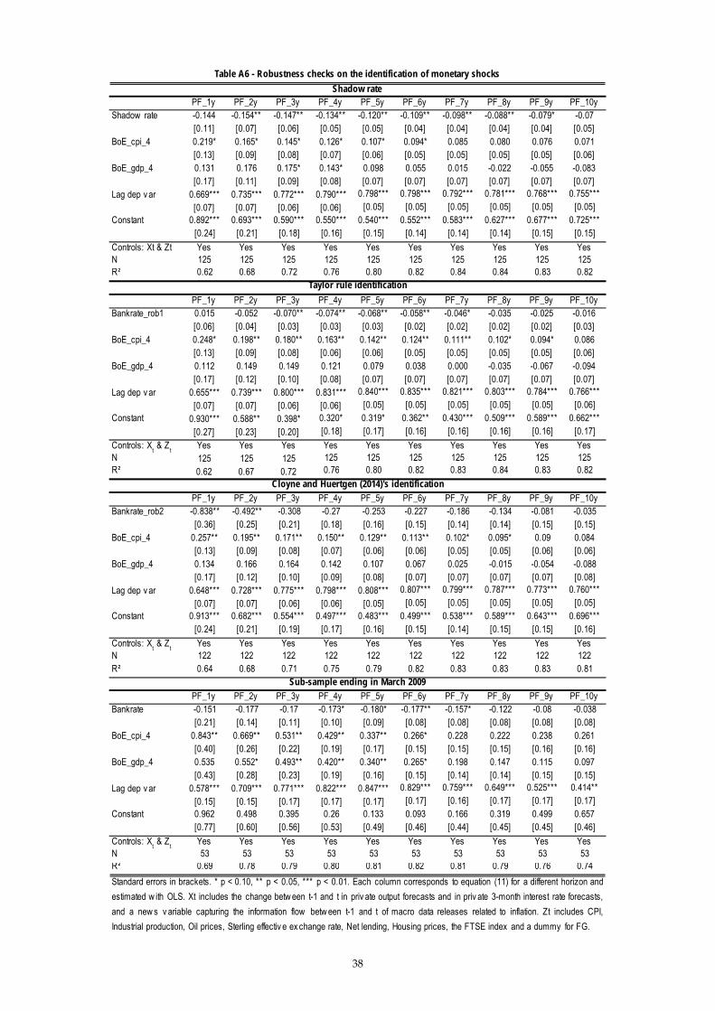
38

PF_1y PF_2y PF_3y PF_4y PF_5y PF_6y PF_7y PF_8y PF_9y PF_10yShadow rate -0.144 -0.154** -0.147** -0.134** -0.120** -0.109** -0.098** -0.088** -0.079* -0.07

[0.11] [0.07] [0.06] [0.05] [0.05] [0.04] [0.04] [0.04] [0.04] [0.05]BoE_cpi_4 0.219* 0.165* 0.145* 0.126* 0.107* 0.094* 0.085 0.080 0.076 0.071

[0.13] [0.09] [0.08] [0.07] [0.06] [0.05] [0.05] [0.05] [0.05] [0.06]BoE_gdp_4 0.131 0.176 0.175* 0.143* 0.098 0.055 0.015 -0.022 -0.055 -0.083

[0.17] [0.11] [0.09] [0.08] [0.07] [0.07] [0.07] [0.07] [0.07] [0.07]Lag dep v ar 0.669*** 0.735*** 0.772*** 0.790*** 0.798*** 0.798*** 0.792*** 0.781*** 0.768*** 0.755***

[0.07] [0.07] [0.06] [0.06] [0.05] [0.05] [0.05] [0.05] [0.05] [0.05]Constant 0.892*** 0.693*** 0.590*** 0.550*** 0.540*** 0.552*** 0.583*** 0.627*** 0.677*** 0.725***

[0.24] [0.21] [0.18] [0.16] [0.15] [0.14] [0.14] [0.14] [0.15] [0.15]

Controls: Xt & Zt Yes Yes Yes Yes Yes Yes Yes Yes Yes YesN 125 125 125 125 125 125 125 125 125 125R² 0.62 0.68 0.72 0.76 0.80 0.82 0.84 0.84 0.83 0.82

PF_1y PF_2y PF_3y PF_4y PF_5y PF_6y PF_7y PF_8y PF_9y PF_10yBankrate_rob1 0.015 -0.052 -0.070** -0.074** -0.068** -0.058** -0.046* -0.035 -0.025 -0.016

[0.06] [0.04] [0.03] [0.03] [0.03] [0.02] [0.02] [0.02] [0.02] [0.03]BoE_cpi_4 0.248* 0.198** 0.180** 0.163** 0.142** 0.124** 0.111** 0.102* 0.094* 0.086

[0.13] [0.09] [0.08] [0.06] [0.06] [0.05] [0.05] [0.05] [0.05] [0.06]BoE_gdp_4 0.112 0.149 0.149 0.121 0.079 0.038 0.000 -0.035 -0.067 -0.094

[0.17] [0.12] [0.10] [0.08] [0.07] [0.07] [0.07] [0.07] [0.07] [0.07]Lag dep v ar 0.655*** 0.739*** 0.800*** 0.831*** 0.840*** 0.835*** 0.821*** 0.803*** 0.784*** 0.766***

[0.07] [0.07] [0.06] [0.06] [0.05] [0.05] [0.05] [0.05] [0.05] [0.06]Constant 0.930*** 0.588** 0.398* 0.320* 0.319* 0.362** 0.430*** 0.509*** 0.589*** 0.662***

[0.27] [0.23] [0.20] [0.18] [0.17] [0.16] [0.16] [0.16] [0.16] [0.17]

Controls: Xt & Z

tYes Yes Yes Yes Yes Yes Yes Yes Yes Yes

N 125 125 125 125 125 125 125 125 125 125R² 0.62 0.67 0.72 0.76 0.80 0.82 0.83 0.84 0.83 0.82

PF_1y PF_2y PF_3y PF_4y PF_5y PF_6y PF_7y PF_8y PF_9y PF_10yBankrate_rob2 -0.838** -0.492** -0.308 -0.27 -0.253 -0.227 -0.186 -0.134 -0.081 -0.035

[0.36] [0.25] [0.21] [0.18] [0.16] [0.15] [0.14] [0.14] [0.15] [0.15]BoE_cpi_4 0.257** 0.195** 0.171** 0.150** 0.129** 0.113** 0.102* 0.095* 0.09 0.084

[0.13] [0.09] [0.08] [0.07] [0.06] [0.06] [0.05] [0.05] [0.06] [0.06]BoE_gdp_4 0.134 0.166 0.164 0.142 0.107 0.067 0.025 -0.015 -0.054 -0.088

[0.17] [0.12] [0.10] [0.09] [0.08] [0.07] [0.07] [0.07] [0.07] [0.08]Lag dep v ar 0.648*** 0.728*** 0.775*** 0.798*** 0.808*** 0.807*** 0.799*** 0.787*** 0.773*** 0.760***

[0.07] [0.07] [0.06] [0.06] [0.05] [0.05] [0.05] [0.05] [0.05] [0.05]Constant 0.913*** 0.682*** 0.554*** 0.497*** 0.483*** 0.499*** 0.538*** 0.589*** 0.643*** 0.696***

[0.24] [0.21] [0.19] [0.17] [0.16] [0.15] [0.14] [0.15] [0.15] [0.16]

Controls: Xt & Z

tYes Yes Yes Yes Yes Yes Yes Yes Yes Yes

N 122 122 122 122 122 122 122 122 122 122R² 0.64 0.68 0.71 0.75 0.79 0.82 0.83 0.83 0.83 0.81

PF_1y PF_2y PF_3y PF_4y PF_5y PF_6y PF_7y PF_8y PF_9y PF_10yBankrate -0.151 -0.177 -0.17 -0.173* -0.180* -0.177** -0.157* -0.122 -0.08 -0.038

[0.21] [0.14] [0.11] [0.10] [0.09] [0.08] [0.08] [0.08] [0.08] [0.08]BoE_cpi_4 0.843** 0.669** 0.531** 0.429** 0.337** 0.266* 0.228 0.222 0.238 0.261

[0.40] [0.26] [0.22] [0.19] [0.17] [0.15] [0.15] [0.15] [0.16] [0.16]BoE_gdp_4 0.535 0.552* 0.493** 0.420** 0.340** 0.265* 0.198 0.147 0.115 0.097

[0.43] [0.28] [0.23] [0.19] [0.16] [0.15] [0.14] [0.14] [0.15] [0.15]Lag dep v ar 0.578*** 0.709*** 0.771*** 0.822*** 0.847*** 0.829*** 0.759*** 0.649*** 0.525*** 0.414**

[0.15] [0.15] [0.17] [0.17] [0.17] [0.17] [0.16] [0.17] [0.17] [0.17]Constant 0.962 0.498 0.395 0.26 0.133 0.093 0.166 0.319 0.499 0.657

[0.77] [0.60] [0.56] [0.53] [0.49] [0.46] [0.44] [0.45] [0.45] [0.46]

Controls: Xt & Z

tYes Yes Yes Yes Yes Yes Yes Yes Yes Yes

N 53 53 53 53 53 53 53 53 53 53R² 0.69 0.78 0.79 0.80 0.81 0.82 0.81 0.79 0.76 0.74

Table A6 - Robustness checks on the identification of monetary shocks

Shadow rate

Taylor rule identification

Cloyne and Huertgen (2014)'s identification

Standard errors in brackets. * p < 0.10, ** p < 0.05, *** p < 0.01. Each column corresponds to equation (11) for a different horizon and

estimated w ith OLS. Xt includes the change betw een t-1 and t in priv ate output forecasts and in priv ate 3-month interest rate forecasts,

and a new s v ariable capturing the information flow betw een t-1 and t of macro data releases related to inflation. Zt includes CPI,

Industrial production, Oil prices, Sterling effectiv e ex change rate, Net lending, Housing prices, the FTSE index and a dummy for FG.

Sub-sample ending in March 2009