Working Paper Series

Research and Statistics Department

Bank of Japan

C.P.O. BOX 203 Tokyo

100-8630 JAPAN

* e-mail: kobayashi-keiichiro@rieti.go.jp

Deposit Money Creation in Search Equilibrium

Keiichiro Kobayashi*

Working Paper 02-4

Views expressed in Working Paper Series are those of authors and do not necessarily reflect those of the Bank of Japan or Research and Statistics Department.

Deposit Money Creation in Search Equilibrium∗

Keiichiro Kobayashi†

June 4, 2002

Abstract

The endogenous creation of bank credit and of deposit money is modeled. If

banks have a limited ability to commit to making interbank loans, then, in order for

bank deposits to be accepted as liquid assets, an upper bound is placed upon the size

of each bank’s asset portfolio, where the bound is determined as a certain multiple

of the bank’s capital. In our search model, the Central Limit Theorem implies that

the multiplier is a non-linear function of the aggregate level of bank assets. Thus

when banks have little capital, there emerges an inefficient equilibrium where the

production level is low and unemployment exists. In the case where the initial value

of bank capital is small and pessimistic macroeconomic expectations prevail, the

economy converges on the unemployment equilibrium even if prices are flexible.

Keywords: Limited ability to commit, the interbank market, the Central Limit

Theorem, search model.

JEL Classification: C72, E44, E51, G21.

∗I wish to thank Hideo Hayakawa, Toshitaka Sekine, Koichiro Kamada, and seminar participants at

the Bank of Japan and the Research Institute of Economy, Trade and Industry (RIETI) for many helpful

comments. I am also grateful for helpful comments from the anonymous referee. All remaining errors

are mine. The views expressed herein are those of the author and not necessarily those of the Bank of

Japan or RIETI.†The Research Institute of Economy, Trade and Industry. E-mail: kobayashi-keiichiro@rieti.go.jp

1

1 Introduction

This is a simple model to illustrate the macroeconomic role of deposit money creation

by banks. We assume the Cash-In-Advance constraint: i.e., that the medium of ex-

change is restricted to cash in this economy. Our purpose in this paper is to model,

within a Cash-In-Advance economic setting, a game theoretic mechanism through which

bank deposits are accepted as liquid assets, and to analyze the macroeconomic effect

of deposit money creation on the real output of the economy. We show that if banks

have incomplete information about withdrawals by depositors and they have no ability

to commit beforehand to lend cash to other banks in the interbank market, then the

dominant strategy for any bank is to refuse to lend cash to other banks. In this case,

the interbank market cannot be formed. If banks have a limited ability to commit, then

the condition for the interbank market to be successfully established is that the size of

bank lending is no larger than a certain multiple of bank capital where the multiplier is

shown to be a function of the aggregate size of bank loans. Thus each bank must limit

its lending to a certain multiple of its capital in order for its deposits to be accepted as

liquid assets.

When looking at real activity, we use a search model setting (Diamond[1982][1984],

Kiyotaki and Wright[1989]) : firms must find trading partners in order to produce final

goods, and they need to carry money when searching. The necessity of search induces

complementarity among activities by firms. This complementarity and the Central Limit

Theorem imply that our credit multiplier (the ratio of outstanding bank loans to bank

capital) is a non-linear function of the aggregate size of bank loans. Therefore, it is

shown that if banks have little capital, there exist multiple equilibria corresponding to

different values of the credit multiplier. In the equilibrium corresponding to the small

credit multiplier, there is unemployment. Given the appropriate parameter values, the

economy converges on the neighborhood of this inefficient equilibrium if the initial value

of bank capital is small and pessimistic macroeconomic expectations prevail.

2

2 Basic Model

In this section, we construct a stylized model to demonstrate the macroeconomic effect

of deposit money creation. In the next section, we generalize the model so that we can

characterize the general equilibrium completely.

2.1 Economic Environment

The model is an infinite period economy that consists of identical consumers, producing

firms, and banks. Time is discrete and goes from zero to infinity. Each consumer is

endowed with one unit of labor at the beginning of every period. The only productive

input is labor, and the consumer good is the only output. The medium of exchange in

this economy is restricted to cash, the amount of which is given exogenously.

Assumption 1 (Cash-In-Advance Constraint) Firms need to use cash to purchase labor

from consumers. Consumers need to use cash to purchase the consumer good.

Timetable In every period t, events take place in the following order. Details of the

events are described in the following subsections unless otherwise noted. Each period t

is divided into three subperiods: the beginning (tb), the intermediate subperiod (ti), and

the end of the period (te).

· Subperiod tb:

(1) Consumers invest their cash Ct in banks. Each consumer is endowed with a unit

of labor that is effective only in period t.

(2) Banks engage in corporate lending or investment in other banks. A firm borrows

wt units of cash where wt is the wage in period t.

(3) Firms deposit the cash in the same bank that they borrowed from1.

(4) Banks establish membership of the interbank market via a game among banks.

1This assumption that firms make deposits in the lender bank is just for simplicity of exposition. Our

result does not change qualitatively even if firms do not make deposits in the original lender, but can

make deposits in any bank.

3

· Subperiod ti:

(5) Firms conduct a search for other firms.

(6) A firm encounters another firm according to a random matching.

(7) After the search activity ends, the following events occur simultaneously (or in

random order):

(7-1) In order to pay wages, matched firms either withdraw their deposits, or

sell their deposit certificates to other banks. Banks accept the deposit certificates if the

issuing banks are members of the interbank market.

(7-2) Firms pay wages to consumers, and produce the consumer good using the

labor input.

(7-3) Consumers divide their wage income equally according to an unemployment

insurance scheme.

(7-4) Consumers deposit their wage income in their bank accounts.

· Subperiod te:

(8) Consumers borrow cash ptct from banks and buy ct units of the consumer good

where pt is the price of the consumer good in period t.2

(9) Firms repay pt to banks (pt > wt).

(10) The interbank market opens to settle interbank loans. Banks that issued deposit

certificates (issuing banks) pay wt to the banks holding their certificates (holder-banks).

(11) Banks pay out the remaining surplus ((1 + rt)Ct + wtλt − ptct) to consumers.3

Consumer There are N consumers who have identical preferences. N is a very large

integer. At the beginning of period t (t = 0, 1, · · · ,∞), each consumer has one unit of

labor and initial wealth Ct in the form of cash, which she invests in the bank as bank

capital. Then a firm employs the consumer with a certain probability (specified later),

and the consumer obtains the wage wt. The consumer may only use her labor to produce

the consumer good if she is employed. Otherwise she cannot produce the consumer good,

since only firms have access to the production technology. For simplicity, we assume that

2See footnote 16.3See footnote 17.

4

there is unemployment insurance among consumers so that labor-income wt is equalized

among all consumers no matter who is employed. Thus each consumer obtains wtλt

where λt is the endogenous probability of being employed (See equation (2)).

After production has taken place, the consumer chooses her consumption for the cur-

rent period (ct). Thus the consumer’s problem is the following. Given {pt, wt, λt, rt}∞t=0

and C0, the consumer solves

maxct

∞∑t=0

βtu(ct)

subject to ptct+Ct+1 ≤ wtλt+(1+rt)Ct, where pt is the price of the consumer good and

rt is the rate of return on the investment in bank capital, while u(·) is a standard utility

function that satisfies u′ > 0 and u′′ ≤ 0. For simplicity, we also assume that consumers

have insurance covering their investments in banks so that each consumer obtains the

same return on her investment Ct. Thus rt is a deterministic number for each consumer.

Firms The number of firms is K where K is a large integer that satisfies K > N .4

We assume that the production technology of one firm is incomplete: a firm is only able

to produce a unit of the consumer good if and only if it meets another firm in the mar-

ket and the two firms exchange information, thus enabling both firms to complete their

production technologies. Therefore, a firm needs to search for another firm before it can

employ the laborer (= the consumer) to produce the consumer goods. This production

technology is a replica of that in Diamond [1982].5 Although this assumption on the pro-

duction technology seems too restrictive, it is one way to formulate the complementarity

among the activities of economic agents that is commonly observed.

A firm needs to borrow cash from a bank when it starts searching. This is because

4The number of firms can be infinite. The existence of the upper limit K is not necessary to derive

our main results.5We can interpret this technology as a technology of trading like that in the Diamond-model. Suppose

that production of the consumer good necessitates a division of labor between two firms. Each firm can

produce only an intermediate good, and the final good is produced by combining two intermediate goods.

In this case, firms need to search for a trading partner with whom to divide the labor of producing the

final good.

5

of the following assumption.

Assumption 2 It is only when two firms match that they become able to employ a

laborer and so produce the consumer good. The firms must pay the wage in the form of

cash before they sell the consumer good. After the firms match, there is no chance before

production for them to borrow cash from banks. Firms do not hold cash initially.

This assumption implies that a firm must borrow wt units of cash from a bank before it

starts searching. As we show in Section 2.2, each bank determines the size of its lending

so that condition (10) in Section 2.2 is satisfied. In this case, all banks join the interbank

market so that the certificates of deposit issued by banks are accepted as perfectly liquid

assets, and all depositors can withdraw their deposits at any time (See Section 2.2).

Therefore, a firm borrows cash (wt) from a bank and deposits the cash in the bank when

it starts searching since it regards the bank deposit as a perfect substitute for cash.6

Search Technology If Lt firms engage in the search activity in period t, then q(Lt)Lt

firms encounter one another according to a random matching process. q(Lt) describes

the probability that a firm makes a successful match in this way.

Assumption 3 The probability q(L) is defined such that 0 ≤ q(L) ≤ 1 and q(L) is a

strictly increasing function of L. If L (> 0) is sufficiently small, then q(L) = κL+ o(L)

where κ > 0 and limL→0 o(L)/L = 0.

This assumption that q(L) is strictly increasing in L is justified as follows: firms search

for one another by walking randomly around a vast field; in such a case, the probability

of encounter is an increasing function of the number of firms.7 Min{q(Lt)Lt, N} firms

6Alternatively, we can assume that firms have a small risk of losing the cash by accident if they carry

it during the search activity. In this case, firms strictly prefer making a deposit to holding cash if they

believe that the bank deposit is perfectly liquid.7A more realistic explanation for the plausibility of Assumption 3 is the following. A firm searches

for a trading partner, who has certain characteristics, by checking the telephone directory. She looks

first in the directory for New York, and if she cannot find a trading partner there, then she looks in

the directory for New Jersey, and so on for other cities. She repeats this process within a limited time

6

can employ workers and produce the consumer good. The amount of the consumer good

produced in period t is also min{q(Lt)Lt, N}.

Banks We assume that there are M banks in the economy. The number of banks M

is a very large integer but is negligibly small compared to N :

1 �M � N. (1)

This assumption that M � N is crucial for the approximation by the Central Limit

Theorem (See Section 2.2). Assuming that banks receive an identical amount of capital,

each bank has NMCt units of cash invested in it by consumers. Given bank capital of

NMCt, a bank can lend wt to at most N

MwtCt firms. Before starting the search, the debtor

firms deposit the cash they borrowed in the bank, since they regard the bank deposit as

perfectly liquid, as long as banks satisfy condition (10) in Section 2.2. Thus, the bank hasNMCt units of cash and N

MCt units of loans to firms on the asset-side of its balance sheet,

and NMCt units of deposits made by firms and N

MCt units of capital on the liability-side.

Since the bank has NMCt units of cash in hand at this stage, it can lend this cash to

other firms and let them in turn make their deposits within its vaults. By iterating this

procedure, a bank can expand its balance-sheet (as long as it can satisfy condition (10)

in Section 2.2). The withdrawal of deposits is specified later. For now, suppose that

banks have made loans to lt firms and that all deposits, Dt, are liabilities to these same

firms. The only condition that a bank must satisfy is Dt = wtlt, where wtlt describes its

total lending to firms. In other words, each bank has wtlt of loans to firms and NMCt of

cash on the asset-side, and wtlt of deposits and NMCt of capital on the liability-side. The

NMCt units of cash on the asset-side are reserves against the withdrawal of deposits. We

assume the following loan contract between banks and firms.

interval. Suppose that it takes a certain time to get hold of a telephone directory, but that it does not

take any time to check it. If the number of firms increases in every city, then the number of firms listed in

the directory also increases. Then the probability that a firm can find a trading partner within a limited

time interval increases. In other words, if there exists increasing returns in the information processing

technology of searchers, then the matching probability q(L) is increasing in the number of searchers L.

7

Assumption 4 If a firm borrows wt units of cash from a bank and deposits it immedi-

ately in the bank, then this deposit is a demand deposit which receives no interest payment.

When the firm makes a deposit, the bank delivers a certificate of deposit with face value

wt to the firm. The issuing bank must pay cash wt in exchange for the certificate at any

time to anybody. After borrowing, the firm starts searching for another firm. When the

firm encounters another firm, it withdraws its deposit wt, pays wage wt to a worker, and

produces one unit of the consumer good using the labor input. After production, the firm

sells the good at price pt. The firm repays pt to the bank at the end of period t. If the

firm does not encounter another firm when searching, then the firm’s deposit of wt and

her debt of wt offset each other at the end of period t.

Since successful firm encounters are generated at random, the number of firms in debt

to a given bank that succeed in employing workers is a random variable. We denote this

random variable by m̃t:

m̃t =lt∑i=1

z̃it,

where z̃it is 1 with probability ηt, and 0 with probability (1− ηt), where ηt is the proba-

bility that a firm runs into another firm and then successfully employs a worker. Since

M � 1, we can approximate the z̃its (i = 1, · · · , lt) to identically and independently dis-

tributed random variables, so that m̃t becomes a random variable that follows a binary

distribution b(lt, ηt). E[m̃t] = ηtlt, and V [m̃t] = (1 − ηt)ηtlt. In the equilibrium, ηt = yt

Lt

where yt = min{q(Lt)Lt, N} describes the number of firms that successfully match and

hence the level of output, and Lt = Mlt is the total number of searching firms in the

economy.

2.2 Liquidity of Bank Deposit

After the process of random matching is complete, matched firms withdraw their deposits

to pay wages to their workers. The total withdrawal from a bank is a random variable

wtm̃t. Payment of wage wt to a worker is done in the form of cash. Total wage wtyt is

divided equally among all consumers as set out in the unemployment insurance scheme.

8

Thus each worker (a consumer) receives the cash wtλt where

λt =ytN, (2)

and she immediately deposits it in her bank account. We assume that the number of

consumers’ accounts is equal for each bank. Therefore, each bank obtains new deposits

of wtyt

M from workers. We can regard a bank as defaulting, i.e. failing to meet the total

demand for withdrawals from it8, if

N

Mxt < X̃t ≡ m̃t − yt

M, (3)

where xt ≡ Ctwt

, E[X̃t] = ηtlt − yt

M , and V [X̃t] = (1 − ηt)ηtlt. In the equilibrium where

lt = LtM , we have E[X̃t] = 0, and V [X̃t] = (1− ηt)ηt Lt

M .

The Central Limit Theorem implies that the random variable W̃ converges in distri-

bution to a random variable that follows the normal distribution N (0, 1) as LtM becomes

a large number, where W̃ is defined by

W̃ =X̃t√

ηt(1 − ηt)LtM

.

The interbank market and withdrawal by firms When matching firms withdraw

wt from their accounts, the total withdrawal for all banks is wtyt, while the total deposit

that workers make is also wtyt. Therefore, if there is an interbank market where banks

can lend and borrow cash to and from one another, then all banks can meet the total

demand for withdrawals by firms.

In this subsection, we derive the main result of our model. In order for banks who

have a limited ability to commit and incomplete information about withdrawers to form

an interbank market, the variance V [X̃t] = (1 − ηt)ηtlt must not exceed an upper limit

that is an increasing function of the bank capital (Ctwt

).8We need to make more technical assumptions about the timing of withdrawals by firms and of deposits

by workers, in order to derive condition (3). The technical assumptions make our model unnecessarily

complicated without making any qualitative difference to the results. Thus we just assume that a bank

defaults if and only if the sum of existing cash ( NM

Ct) and incoming cash (wtyt

M) is less than outlay

(wtm̃t).

9

The intuition is the following. Consider the game among banks in which they choose

either to agree or to refuse to lend cash to one another when their depositors (firms)

withdraw wt. Suppose that a bank (bank i) cannot commit beforehand to lend cash to

other banks. In this case, bank i can obtain a non-negative surplus by refusing to lend

cash to other banks no matter what the other banks’ strategy is: a bank is strictly better

off by refusal, if all the other banks refuse to lend cash to one another; at the same time,

if some banks agree to lend cash to bank i while bank i refuses to lend cash to other

banks, then bank i can use all of its own cash in addition to those banks’ cash in order

to meet withdrawals by its depositors. Therefore, the dominant strategy for a bank is to

refuse to lend cash to other banks. Thus banks that have no ability to commit cannot

form an interbank loan market.

Suppose, however, that banks have a limited ability to commit: a bank incurs the

penalty ε (> 0) if it breaks its precommitment to lend to other banks. In this case, if the

surplus that a bank can obtain by refusal is no greater than ε, then the interbank market

in which all banks agree to lend to all other banks becomes a Nash equilibrium. The

condition that the surplus from refusal is no greater than ε is shown to be V [X̃t] ≤ φ(Ctwt

)

where φ(·) is a positive and increasing function.

In the following, we formalize the intuition described above.

A game of interbank market formation We assume that the following interbank

game is played after lending (wtlt) is determined, the matchings of firms are realized,

and all workers have deposited their wage income in their bank accounts9.

In the first stage of the game, firms who succeeded in matching form a queue. The

order of the firms in the queue is random. The i-th firm (i = 1, 2, · · · ,∑M1 m̃k.) from

the head of the queue goes to the bank [i]M where [i]M = k satisfies 1 ≤ k ≤ M

and i = mM + k for a non-negative integer m. We assume the following incomplete

information for banks:

9The deposit of wage income (wtytM per bank) must be made simultaneously with the withdrawal by

firms. But in order to simplify the argument, we assume that all workers deposit their wages before firms

start to withdraw their deposits. It is easily confirmed that this simplification does not affect the result.

10

Assumption 5 A bank cannot observe whether the firms remaining in the queue are the

bank’s own depositors or not.

In the second stage of the game, a bank (bank k) either give cash wt to the i-th firm

([i]M = k) or not. If firm i is a depositor of bank k, then bank k has no choice other than

to pay wt to the firm in exchange for its certificate of deposit. If firm i is the depositor of

bank k′ (k′ �= k), then bank k can choose whether to agree or to refuse to give cash wt to

firm i in exchange for the certificate of deposit issued by bank k′. If bank k accepts the

deposit certificate held by firm i, then bank k gives cash wt to firm i. Bank k sends this

deposit certificate to bank k′ in the final stage (i.e., the settlement stage) of the game,

and bank k′ pays cash wt to bank k in exchange for the deposit certificate10. If bank

k rejects the deposit certificate held by firm i or bank k runs out of cash before firm i

comes, then firm i is left with no cash in hand.

The third stage of the game starts after all firms in the queue have visited some bank.

In the third stage, the remaining firms who failed to obtain cash form a second queue.

They form the queue in random order. The procedures for the first and second stage are

then repeated.

We can make the following observation concerning bank strategy. A bank (bank

k) will be weakly better off by refusing to accept deposit certificates issued by other

banks as long as its own depositors remain in the queue. This is because bank k can

spare cash for withdrawals by its own depositors who remain in the queue by rejecting

10Firm i repays pt(> wt) to bank k′ after it sells the consumer good. Thus it might seems natural

to assume that bank k and bank k′ split the surplus pt − wt equally. However, the assumption that

bank k′ pays wt to bank k means that all surplus (pt − wt) is taken by bank k′ (i.e., the original lender

to firm i). This assumption is justified as follows: it is plausible to regard bank lending as a form of

relationship lending in which the original lender obtains an information rent (See, for example, Diamond

and Rajan[2001]). Before the game starts, bank k′ provided the relationship lending for firm i. Thus we

regard (at least a part of) the surplus pt − wt to be the information rent to bank k′, which cannot be

transferred to bank k.

Although we assume for simplicity that bank k′ (the original lender) takes all the surplus, the qualitative

nature of our result does not change as long as bank k′ takes a larger part of the surplus pt − wt than

bank k.

11

other banks’ depositors, while successful withdrawals by its own depositors give positive

surplus to bank k (the original lender). This observation and the information asymmetry

(Assumption 5) justify the following restriction on the choice by banks:

Assumption 6 A bank that decides to reject a certificate of deposit issued by another

bank continues to reject all such certificates for the rest of the game.

It is easily confirmed that banks always agree to establish an interbank market, i.e., the

first best outcome, if they have complete information about withdrawers and they can

change their strategies over the sequence of the game.

This three-stage subroutine is repeated until either (1) all cash has been given to

firms, (2) all firms in the original queue have obtained cash, or (3) all the remaining cash

is possessed by banks that refuse to give cash to firms holding the deposit certificates of

other banks, and all remaining firms are depositors of banks who no longer possess cash.

The final stage (i.e., the settlement stage) takes place after the production and sale

of the consumer good by firms. Bank k that gave cash wt to firm i in exchange for the

deposit certificate issued by bank k′ sends the certificate to bank k′, and bank k′ pays

cash wt to bank k in exchange for the certificate.

The Prisoners’ Dilemma in formation of the interbank market In the above

game, banks choose their strategies simultaneously at the beginning of the game. The

strategy for bank k is to specify whether it accepts or rejects the certificates of deposit

issued by bank k′ (k′ �= k, k′ ∈ {1, 2, · · · ,M}). Simultaneous and independent choice of

strategy by individual banks makes the situation that we should analyze quite compli-

cated: for example, bank 1 accepts11 bank 2 but rejects bank 3; bank 2 accepts bank 3

but rejects bank 1; and bank 3 accepts bank 1 but rejects bank 2.

In order to avoid this complication of the analysis, we assume that banks form an

interbank market according to the process described below:

11We say “bank k accepts (rejects) bank k′,” when bank k agrees (refuses) to give cash wt to anybody

in exchange for the deposit certificate issued by bank k′.

12

Assumption 7 Let Group [1, k − 1] denotes the group that consists of banks 1 through

to k − 1 (k = 2, · · · ,M) where any pair of the member banks of the group accept each

other. The interbank market is formed by the following iteration. (i) Assume that Group

[1, k − 1] acts as a unanimous agent whose objective is to maximize per capita payoff

of its member banks; (ii) Bank k and Group [1, k− 1] simultaneously decide whether to

accept or to reject each other12; (iii) If they accept each other, then bank k and Group

[1, k − 1] merges and they become Group [1, k]. If this iteration is repeated successfully

from k = 2 to k = M , then all M banks join together to form the interbank market, i.e.,

Group [1,M ].

Now, we show that banks that do not have the ability to commit beforehand cannot

form an interbank market.

Lemma 1 In the case where banks have no ability to commit to accept other banks

beforehand, the dominant strategy for bank k is to reject Group [1, k − 1] for all k ∈{2, 3, · · · ,M}.

Proof

Case (i): k = M .

The game between bank M and Group [1,M−1] is a simultaneous game with two choices

of strategy: A (accept) or R (reject). Note that every bank has fixed its asset size (wtlt)

beforehand. If both bank M and Group [1,M − 1] accept each other, then each bank k

(k = 1, · · · ,M) obtains the expected value of the surplus (pt − wt)E[m̃t] = (pt − wt) yt

M .

If both choose rejection, then condition (3) and the Central Limit Theorem imply that

bank M ’s expected surplus is

(pt −wt){∑Nxt

M+

ytM

m=1 mPr{m̃t = m} +(NxtM + yt

M

)Pr{m̃ > Nxt

M + yt

M }}

≈ (pt −wt){E[m̃t] −∫∞

NxtM

(X̃t − N

M xt)dFX(X̃t)}

= (pt −wt){ yt

M − σtΨ(NxtMσt

)}

(4)

12Assume that both bank k and Group [1, k − 1] make the decision on the premise that bank i and

bank j reject each other for any pair of i and j where i ∈ {1, 2 · · · , k} and j ∈ {k + 1, k + 2, · · · , M}.

13

where

σt ≡√V [X̃t] =

√(1− ηt)ηtlt, (5)

and

Ψ(z) =∫ ∞

z(y − z)

1√2πe

−y2

2 dy. (6)

Thus

Ψ(z) =1√2πe−

z2

2 − z(1 − Φ(z)), where Φ(z) =∫ z

−∞1√2πe−

y2

2 dy. (7)

In this case, the condition for default by Group [1,M − 1] approximates to

N

Mxt < X̃M−1, where X̃M−1 ∼ N

(0,

1√M − 1

σt

), (8)

since X̃M−1 = 1M−1

∑M−1k=1 X̃k where X̃k is defined in (3) and is approximately normally

distributed N (0, σt).13 Thus the surplus for a member bank of Group [1,M − 1] can be

approximated by (pt −wt){ yt

M − σt√M−1

Ψ(Nxt

√M−1

Mσt

)}.

If Group [1,M − 1] chooses A while bank M chooses R, then bank M obtains (pt −wt) yt

M , i.e., the same surplus as in the case where both choose A. This is because all

depositors of bank M in the queue obtain cash in exchange for the certificates issued by

bank M . At the same time, a member bank of Group [1,M − 1] obtains strictly less

surplus than in the case where both choose R.

If Group [1,M−1] chooses R while bank M chooses A, then a member bank of Group

[1,M − 1] obtains strictly greater surplus than in the case where both choose A, while

bank M obtains strictly less surplus than in the case where both choose R.

Therefore, the dominant strategy for both bank M and Group [1,M − 1] is R.

Case (ii): k < M .

Note that banks k + 1, k + 2, · · · ,M reject banks 1, 2, · · · , k. Thus bank k and Group

[1, k−1] decide their strategies without influence from banks k+1, · · · ,M . If both bank

k and Group [1, k− 1] accept each other, then the condition for default by Group [1, k]

13To be more precise, the random variables X̃k (k = 1, 2, · · · , M) are not mutually independent, since∑M

1X̃k = 0. However, we can approximate the distribution of X̃M−1 with that of a normal random

variable distributed N(0, σt

M−1

).

14

approximates toN

Mxt < X̃k, where X̃k ∼ N

(0,

1√kσt

). (9)

Thus the payoff for bank k and for a member bank of Group [1, k − 1] are the same:

(pt −wt){ yt

M − σt√kΨ(Nxt

√k

Mσt)}.

If both bank k and Group [1, k − 1] reject each other, then the payoff for bank

k is (pt − wt){ yt

M − σtΨ(NxtMσt

)}.The payoff for a member bank of Group [1, k − 1] is

(pt −wt){ yt

M − σt√k−1

Ψ(Nxt√k−1

Mσt)}.

If bank k chooses R while Group [1, k− 1] chooses A, then bank k obtain the same

benefit as in the case when both choose A: i.e., a depositor of bank k who comes across

a bank in Group [1, k − 1] can get cash in exchange for the deposit certificate of bank

k, generating the surplus pt − wt for bank k. In addition to this, bank k can use all its

cash exclusively to meet the withdrawals made by its own depositors. Thus the surplus

for bank k is strictly greater than the payoff in the case when both choose A. A similar

logic implies that a member bank of Group [1, k− 1] obtains strictly less surplus than in

the case when both choose R.

If bank k chooses A while Group [1, k− 1] chooses R, then the payoff for a member

bank of Group [1, k−1] is strictly greater than in the case when both choose A. Meanwhile

bank k obtains strictly less surplus than in the case when both choose R.

Therefore, the dominant strategy for both bank k and Group [1, k− 1] is R. (End of

Proof )

This lemma implies that the game among banks has a unique Nash equilibrium in

which all banks choose to reject all other banks. Thus banks that do not have the

ability to commit beforehand cannot form an interbank market when they lack complete

information concerning withdrawers (Assumption 5).

Formation of the interbank market under limited ability to commit Now we

assume that banks have a limited ability to commit:

Assumption 8 A bank incurs the fine ε if it rejects deposit certificates issued by banks

15

which it had promised to accept. The fine ε is an exogenous parameter for the bank.

In this case, we can show the following lemma:

Lemma 2 In the case where banks have a limited ability to commit, the sufficient condi-

tion for the existence of an equilibrium in which both bank k and Group [1, k− 1] accept

each other for all k ∈ {2, 3, · · · ,M} is

θt ≡ σt√2Ψ

(Nxt

√2

Mσt

)≤ ε

pt −wt. (10)

(Proof )

It is sufficient to examine the case where k = 2. Both bank 1 and bank 2 obtain

(pt − wt){ yt

M − θt} respectively by accepting each other. Suppose one bank (bank 1)

deviates from this strategy and rejects bank 2, while bank 2 accepts bank 1. In this case,

bank 2 gives cash wt whenever bank 2 comes across a depositor of bank 1, generating

the surplus pt − wt for bank 1, and bank 1 uses all its cash exclusively to meet the

withdrawals made by its own depositors. In this case, the value of bank 1’s expected

surplus is in between (pt − wt){ ytM − θt} and (pt − wt) yt

M . Since bank 1 incurs the fine ε

by deviation, bank 1 always accepts bank 2 as long as bank 2 accepts bank 1 in the case

when condition (10) is satisfied. Therefore, that the both banks accept each other is a

Nash equilibrium of the game between bank 1 and bank 2. For the case of bank k and

Group [1, k− 1] where k > 2, the surplus that a bank can obtain by deviation is smaller

than θt. Thus condition (10) is sufficient. (End of Proof )

This lemma guarantees the existence of a Nash equilibrium in which all banks accept

all other banks. Note that this is not the unique Nash equilibrium. There exists another

Nash equilibrium in which all banks reject all other banks, as long as ε is negligibly

smaller than yt

2M .

16

2.3 Equilibrium Lending

Banks determine the volume of lending wtlt so that condition (10) is satisfied. Condition

(10) can be rewritten as follows since Ψ(z) is a strictly decreasing function.

N

Mxt ≥ Ψ−1

(ε√

2(pt − wt)

√(1 − ηt)ηtlt

) √(1− ηt)ηtlt√

2. (11)

The right hand side is an increasing function of√

(1 − ηt)ηtlt. Since ηt = yt

Ltwhere

yt = min{q(Lt)Lt, N}, solving this condition with equality gives the bank’s choice of lt

as a function of Lt : lt = F (Lt).

To simplify the exposition, we assume the following:

Assumption 9 The fine ε is proportional to the surplus from one lending (pt−wt) times

standard error in the number of withdrawals (√

(1 − ηt)ηtlt). Thus

ε = ξ(pt − wt)√

(1 − ηt)ηtlt,

where ξ is a constant.

In this simplified case, condition (11) requires that NM xt be proportional to

√(1 − ηt)ηtlt.

Thus condition (11) can be rewritten as

N

Mxt = G

√ηt(1− ηt)

L

M, (12)

where G is a positive constant and G increases as ξ decreases. The constant G represents

the inefficiency of the interbank market, i.e., the difficulty for banks to commit.

In the symmetric equilibrium where all banks choose the same volume of lending,

each bank chooses lt = LtM that satisfies (12) in order to be accepted as a member of

the interbank market. Given that banks form the interbank market, the bank does not

default, but can meet the full demand for withdrawals by depositors even in the case

where X̃t becomes large enough to satisfy (3).

Since ηt = q(Lt) for Lt ≤ L0 and ηt = NLt

for Lt ≥ L0 where L0 is determined by

N = q(L0)L0, equilibrium lending is determined by

Lq(L)(1− q(L)) =N 2

G2Mx2t if L ≤ L0 (13)

1− N

L=

N

G2Mx2t if L0 ≤ L ≤ K, (14)

17

and L = K if neither (13) nor (14) is satisfied by any value of L between 0 and K.

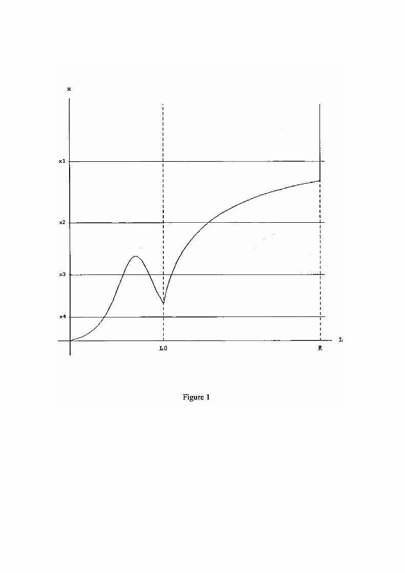
Multiple equilibria emerge for appropriate values of bank capital Ct and wt. See Figure

1.

Figure 1: Equilibrium Lending

In Figure 1, the parameter values are chosen as follows: q(L) = 11+exp{− 1

10(L−70)} , N =

100, M = 50, and G = 60.14

When xt ≡ Ctwt

is sufficiently large (xt = x1), then Lt goes to the upper bound:

Lt = K. When xt = x2, then there exists a unique equilibrium L∗h. When xt is chosen

to be appropriately small (xt = x3), then there emerges three equilibrium values for

lending: L∗h, L

∗m, and L∗

l where L∗l < L∗

m < L∗h. When xt is sufficiently small (xt = x4),

there exists only one equilibrium L∗l .

We examine the stability of the various values for equilibrium lending L∗. Since banks

determine the volume of lending via lt = F (Lt) taking Lt as given, we can say that L∗

is stable if F ′(L∗) < 1M . This is because, if F ′(L∗) < 1

M , then lt goes back to L∗M when

Lt deviates slightly from L∗. We then have the following result concerning stability:

Lemma 3 The equilibrium value L∗l that occurs when xt = x3 or xt = x4 is stable; L∗

h

that occurs when xt = x2 or xt = x3 is also stable; L∗m that occurs when xt = x3 is

unstable.

See the Appendix for the proof. This lemma implies that, for appropriately small values

of Ctwt

, there exist multiple equilibria, which are stable against small perturbations in L.

The Equilibrium Production The search technology implies that the equilibrium

output is

y∗t = min{q(L∗t )L

∗t , N}. (15)

In the cases when xt = x1 or xt = x2 (Figure1), the equilibrium output satisfies y∗ = N

and there is no unemployment. In the case when xt = x3 and L∗ = L∗l , output is

14In Figures 1, 2 and 3, we normalize L, M and N so that our approximation by the Central Limit

Theorem is effective in the figures. Thus we regard, for example, 1 unit of L or N to be equivalent to 1

million firms or consumers respectively, and 1 unit of M to 1000 banks.

18

y∗l = q(L∗l )L

∗l (< N ) and there is unemployment. y∗l is stable against small perturbation

in lending L∗t .

Discussion We have shown that a stable unemployment equilibrium exists if the value

of Ctwt

is small. Our simple model implies that the micro level constraint on bank lending

to maintain the liquidity of deposit money (condition (12)) determines macroeconomic

performance via a stochastic mechanism, i.e., the Central Limit Theorem.

In this economy, a shortage of bank capital induces unemployment.15 Such a shortage

of bank capital may occur in several ways. One example is through currency crises. When

the domestic currency undergoes a sharp devaluation, banks run short of capital if they

have assets denominated in the domestic currency while they have liabilities denominated

in a foreign currency. Another example might be the bursting of an asset price bubble

in the real estate or stock market. If banks have corporate loans the value of which is

determined by the assets that debtor firms own, and if debtor’s assets consist of real

estate and other firms’ stocks, then the bursting of an asset price bubble devalues banks’

assets abruptly, causing a shortage of bank capital.

One can criticize this story by saying that even if nominal bank capital Ct is impaired,

a fall in the wage rate wt will restore the value of Ctwt

so that the economy can return

to full employment. We need to construct a more complete model in order to analyze

the general equilibrium effects of a price change (See the next section). Here we merely

suggest one possible defense against this argument: the stickiness of wages compared to

currency or asset prices. Exchange rates and asset prices are quite volatile. Thus half of

a bank’s capital can be wiped out in a very short period of time, while it takes a very

long time to reduce the nominal wage by half. As a result, the inefficiency caused by the

shortage of bank capital continues for a long period of time.

In the next section, we show that, even if the wage is not sticky, the inefficient

equilibrium exists and the economy may stay in its neighborhood forever.

15We may interpret Ct as the high-powered money provided by the central bank. However, in our

model we do not specify how the central bank controls the amount of Ct, the investment by consumers

in bank capital. Further research is necessary to clarify the role of the monetary policy in our model.

19

3 General Equilibrium and Equilibrium Dynamics

In the previous section, we have shown that the unemployment equilibrium exists if Ctwt

is sufficiently small. The question in this section is whether a flexible change in the

wage wt can restore the high value of Ctwt

, leading the economy to the full employment

equilibrium. In this section we show that, even if wt is flexible, the value of Ctwt

that

supports the unemployment equilibrium is realized in general equilibrium, and that the

economy converges to the bounded neighborhood of the unemployment equilibrium from

a wide range of initial values of C0w0

.

Existence of Unemployment Equilibrium Given the equilibrium output yt and

the equilibrium lending Lt, the consumer solves

maxct

∞∑t=0

βtu(ct) (16)

subject to ptct + Ct+1 ≤ wtλt + (1 + rt)Ct. The consumers’ choice of ct takes place in

subperiod te (See Timetable in Section 2). Consumers borrow cash ptct from banks and

buy consumer goods16; firms that sold the consumer goods repay pt to banks; banks pay

out (1 + rt)Ct + wtλt − ptct to each consumer.17

The first order condition for the consumer’s problem is

ptpt+1

(1 + rt+1) =u′(ct)

βu′(ct+1). (17)

The equilibrium conditions are ct = yt

N and λt = yt

N . The number of unknowns (pt, ct,

Ct+1, rt, λt) is larger than the number of equations (the budget constraint, the first order

condition and the equilibrium conditions). Thus there are infinite equilibria. In order to

specify the equilibrium, we assume the existence of an asset market:

16 To be precise, we need also to consider interbank lending in order for banks to meet consumers’

demand for borrowing given the supply of firms’ repayment. But to simplify the argument, we just

assume that the interbank market works well, and that there is no risk of bank default in this stage.17 In equilibrium, rtCt = ptct − wtλt. Thus the bank pays out Ct units of cash to each consumer,

which is the exact amount of cash that the consumer invested in the bank at tb.

20

Assumption 10 Instead of lending cash to a firm, a bank can invest its cash in another

bank’s capital, where the rate of return is rt.

This assumption in our simple economy is equivalent to assuming that there exists a

bond market or a stock market in which consumers or banks can invest their money.

The existence of an asset market implies that arbitrage between the asset market and

corporate lending occurs. In this case, we have the following arbitrage condition:

1 + rt =ptηtwt

. (18)

In the steady state equilibrium where 1 + rt = β−1 holds, the budget constraint for the

consumer problem implies

Ctwt

=

(β−1

ηt− 1

)yt

N

β−1 − 1(19)

=

(β−1−q(L)β−1−1

)LN if L ≤ L0

LNβ−1−1

β−1−1if L > L0

(20)

The conditions for equilibrium lending ((13) and (14)) and (19) determine the equilibrium

pair, C∗

w∗ and L∗. See Figure 2.

Figure 2: Multiple Equilibria

In Figure 2, we set β = 0.95, while we use the same values as Figure 1 for the other

parameters. For a wide range of parameter values, there are two or more equilibria: some

equilibria corresponding to unemployment and others to full employment. Note that if

the parameter G is sufficiently small, then the unemployment equilibrium vanishes and

full employment is always attained in steady state. Figure 3 shows that there is a unique

equilibrium in which full employment is attained when G is small. In Figure 3, G = 7,

while the other parameters are the same as Figure 2.

Figure 3: Efficient Equilibrium

Recall that 1ML = F (L) has two stable solutions: L∗

l and L∗h when Ct

wtis small (See

Figure 1). We can denote them as L∗l (xt) and L∗

h(xt) where xt ≡ Ctwt

, since (13) and

21

(14) imply that L∗l and L∗

h can be regarded as functions of xt. Equilibrium lending in

the unemployment equilibrium is L∗l (x

∗l ) where x∗l is the value of C∗

w∗ that produces the

equilibrium shown in Figure 2 as the intersection of (13) and (19).

Equilibrium Dynamics and Stability of the Steady State We examine whether

an economy initially apart from the steady states converges to the steady state equilib-

rium (x∗l ) specified above.

Suppose that the economy is apart from the steady states at time t. Since the profits

of bank shareholders must equal the total bank profit from corporate lending, we have

rtCt = (pt − wt)ytN

(21)

This condition and the budget constraint for the consumer imply that Ct = Ct+1, which

can be rewritten asptpt+1

=Ct+1

wt+1

pt

wt

Ctwt

pt+1

wt+1

. (22)

Conditions (18) and (21) implyptwt

=xt − yt

N

xtηt − yt

N

(23)

where xt = Ctwt

. Conditions (17) and (18) imply

u′(ct)βu′(ct+1)

=ptpt+1

pt+1

wt+1ηt+1. (24)

Together, conditions (22), (23) and (24) imply

u′(ct+1)xt+1ηt+1 = β−1u′(ct)xtηt

(xt − yt

Nηt

xt − yt

N

), (25)

where ct = ηtLt/N , ηt = q(Lt) if Lt ≤ L0 and ηt = NL if Lt > L0, and Lt = L(xt)

which is the solution of 1ML = F (L). Note that whether Lt = L∗

l (xt) or Lt = L∗h(xt) is

realized depends upon expectations. Since our purpose is to examine the stability of the

unemployment equilibrium that corresponds to L∗ = L∗l (x

∗l ), we restrict our attention

to the case where people’s expectations are coordinated to realize Lt = L∗l (xt). In this

case, ηt = q(L∗l (xt)) and yt = L∗

l (xt)q(L∗l (xt)), since L∗

l (xt) < L0. Thus (25) is rewritten

as

J(xt+1) = β−1H(xt)J(xt), (26)

22

whereJ(x) ≡ u′

(L∗

l(x)q(L∗

l(x))

N

)xq(L∗

l (x)), and

H(x) ≡(x− L∗

l(x)

N

)/(x− L∗

l(x)q(L∗

l(x))

N

).

Difference equation (26) determines xt+1 as a function of xt. We denote this as

xt+1 = G(xt). The unemployment equilibrium x∗l is the solution of x = G(x) (It is easily

shown that (19) is derived by setting xt+1 = xt, ct+1 = ct and ηt+1 = ηt in (25)). We

can prove the following proposition.

Proposition 1 Assume that u(c) = c1−θ−11−θ . Assume appropriate parameter values such

that

(a) 1 − 1G√Mκ

> β,

(b) 0 < x∗l < x, where x is defined by dL∗l (x)dx <

L∗l (x)x for all x ∈ (0, x),

(c) x∗l < x̂ < x where x̂ is defined by J(x̂) = β−1J(x∗l ), and

(d) J(x) �= β−1J(x)H(x) for x ∈ (x∗l , x̂).

Define x by

J(x) = infx∗

l≤x≤x̂

β−1J(x)H(x).

Then the sequence {xt}∞t=0 converges to the region [min{x∗l , x}, x̂] as t goes to infinity, if

x0 ∈ (0, x̂) and xt+1 is determined by (26).

(Proof )

Since u(c) = c1−θ−11−θ , J(x) = N θ{L∗

l (x)}−θxq(L∗l (x))

1−θ. It is easy to show that {L∗l (x)}−θx

is an increasing function of x if dL∗l (x)

dx <L∗

l (x)

x . Therefore, J(x) is an increasing function

of x if 0 < x < x.

Next, we compare the values of J(x) and β−1J(x)H(x) for values of x close to 0.18 We

can calculate the value ofH(x) evaluated at x = 0 by L’Opital’s rule: limx→0 H(x) = 1−

18In the following argument, we use the approximation that x and L are small numbers, although we

derived the functional form of L∗l (x) by the Central Limit Theorem assuming that L is a large number.

The justification for this approximation that L is small comes from our normalization of the units of L:

i.e., that 1 unit of L equals, for example, 1 million firms. Thus we can assume that even a small L is

large enough for us to be able to use the Central Limit Theorem to derive L∗l (x).

23

1N∂L∂x |x=0. Since q(L) = κL+o(L) for small L, condition (13) implies that L(x)q(L(x)) ≈

κL2 ≈ N2

G2M x2. Thus ∂L∂x |x=0 = N

G√Mκ

. Therefore,

limx→0

H(x) = 1 − 1G√Mκ

. (27)

In the neighborhood of x = 0, difference equation (26) can be rewritten as

J(xt+1) ≈ β−1(1 − 1

G√Mκ

)J(xt). (28)

Since 1− 1G√Mκ

> β is satisfied, J(xt+1) = β−1J(xt)H(xt) > J(xt) for sufficiently small

xt, and therefore xt+1 > xt.

We have β−1J(x)H(x) > J(x) for all x ∈ (0, x∗l ), since x∗l is the smallest positive

solution for β−1J(x)H(x) = J(x). Since β−1J(x)H(x) < β−1J(x) for all x > 0, the con-

tinuity of J(x) and H(x) in the region 0 < x < x implies convergence to [min{x∗l , x}, x̂].(end of Proof )

Therefore, if the parameter values are chosen appropriately, the economy converges

to the closed neighborhood of x∗l from a small value of x0. Moreover, if β−1J(x)H(x)

is increasing in x for ∀x ∈ (x∗l , x̂), then the economy converges to the unemployment

equilibrium x∗l if the initial value x0 ∈ (0, x̂) and macroeconomic expectations are coor-

dinated so that Lt = L∗l (xt) is satisfied. In this case, the unemployment equilibrium is

stable.

4 Conclusion

In our simple model, the size of the bank’s asset portfolio must not exceed a certain

multiple of its capital in order for deposits at the bank to be accepted as liquid assets.

The complementarity between firms in the production technology and this microeconomic

restriction on deposit money creation produce an unemployment equilibrium.

The policy implication of our model are subtle. In our model, if the initial value of

x0 = C0w0

is small and macroeconomic expectations are pessimistic (Lt = L∗l (xt)), then

the economy converges on the neighborhood of the unemployment equilibrium x∗l . To

24

overcome the weight of pessimistic expectations, it might be effective to augment bank

capital with a lump-sum transfer from consumers to banks. If bank capital is augmented

and xt becomes large enough, then L∗l vanishes and the only value for equilibrium lending

that remains is L∗h (See the case when xt = x1 in Figure 1).

A further policy implication concerns prudential regulation for maintaining the liq-

uidity of deposit money. In our model, if the parameter G is small, then the inefficient

equilibrium vanishes. The parameter G, representing the inefficiency of the interbank

market, determines the macroeconomic efficiency of the economy. The factors that de-

termine G include, for example, unambiguity in the stance of the regulatory authorities

concerning bank failure. Thus the maintenance of efficient bank regulation is a necessary

condition for preventing the emergence of the unemployment equilibrium.

Appendix

Proof of Lemma 2

We will prove that F ′(L∗l ) <

1M , F ′(L∗

h) <1M , and F ′(L∗

m) > 1M . At L = L∗

l , the function

ψ(L) = Lq(L)(1−q(L)) is increasing. Suppose that L increases infinitesimally, becoming

L∗l + δ. Suppose that, given the social level of lending L∗

l + δ, a individual bank chooses

lt = 1M (L∗

l + δ). Then θ( 1M (L∗

l + δ), q(L∗l + δ)) =

∫∞NMx

(X̃δ − N

M x)f(X̃δ)dX̃δ, where

X̃δ ∼ N

(0,√ψ(L∗

l+δ)

2M

). On the other hand, θ( 1

ML∗l , q(L

∗l )) =

∫∞NMx

(X̃ − N

M x)f(X̃)dX̃,

where X̃ ∼ N

(0,√ψ(L∗

l)

2M

). Since ψ(L) is increasing at L = L∗

l , it is the case that

ε = θ( 1ML∗

l , q(L∗l )) < θ( 1

M (L∗l + δ), q(L∗

l + δ)). Since θ(lt, ηt) is increasing in lt, lt

must be smaller than 1M (L∗

l + δ), in order to satisfy (11) given Lt = L∗l + δ. Thus,

lt = F (L∗l + δ) < 1

M (L∗l + δ), which implies F ′(L∗

l ) <1M . At L = L∗

h, the function

ψ(L) = LNL

(1 − N

L

)is increasing. By a similar argument we can show that F ′(L∗

h) <1M .

Since ψ(L) is decreasing at L = L∗m, the same logic implies that F ′(L∗

m) > 1M .

25

References

Diamond, D.W. and R.G. Rajan (2001), “Liquidity Risk, Liquidity Creation, and Finan-

cial Fragility: A Theory of Banking,” Journal of Political Economy, 109: 287-327.

Diamond, P. (1984), “Money in Search Equilibrium,” Econometrica, 52: 1-20.

— (1982), “Aggregate Demand Management in Search Equilibrium,” Journal of Political

Economy, 90: 881-894.

Kiyotaki, N. and R. Wright (1989), “On Money as a Medium of Exchange,” Journal of

Political Economy, 97: 927-54.

26