working paper series - european central bank · 1 i especially thank without implicating francisco...
TRANSCRIPT
WORK ING PAPER S ER I E SNO. 371 / J UNE 2004
INFLATION PERSISTENCE:
FACTS OR ARTEFACTS?
by Carlos Robalo Marques
EUROSYSTEM INFLATION PERSISTENCE NETWORK

In 2004 all publications
will carry a motif taken
from the €100 banknote.
WORK ING PAPER S ER I E SNO. 371 / J UNE 2004
INFLATION PERSISTENCE:
FACTS OR ARTEFACTS? 1
by Carlos Robalo Marques 2
1 I especially thank without implicating Francisco Dias, Maximiano Pinheiro, Pedro Neves, Nuno Alves and José Maria Brandão de Brito for helpful discussions. Useful suggestions from Benoît Mojon,Andrew Levin, Jordi Gali and other members of the
Inflation Persistence Network (IPN) are also acknowledged.The usual disclaimer applies.2 Banco de Portugal.
This paper can be downloaded without charge from http://www.ecb.int or from the Social Science Research Network
electronic library at http://ssrn.com/abstract_id=533131.
EUROSYSTEM INFLATION PERSISTENCE NETWORK

© European Central Bank, 2004
AddressKaiserstrasse 2960311 Frankfurt am Main, Germany
Postal addressPostfach 16 03 1960066 Frankfurt am Main, Germany
Telephone+49 69 1344 0
Internethttp://www.ecb.int
Fax+49 69 1344 6000
Telex411 144 ecb d
All rights reserved.
Reproduction for educational and non-commercial purposes is permitted providedthat the source is acknowledged.
The views expressed in this paper do notnecessarily reflect those of the EuropeanCentral Bank.
The statement of purpose for the ECBWorking Paper Series is available from theECB website, http://www.ecb.int.
ISSN 1561-0810 (print)ISSN 1725-2806 (online)
3ECB
Working Paper Series No. 371June 2004
CONTENT S
Abstract 4
Non-technical summary 5
1. Introduction 6
2. Defining and measuring inflation persistence 7
2.1. Defining inflation persistence 7
2.2. Measures of inflation persistence 10
3. Persistence and mean reversion 14
4. An alternative measure of persistence 19
5. Persistence and mean reversion: re-evaluatinginflation persistence in the United States andthe euro area 20
6. Conclusions 31
References 32
Appendices 35
Graphics and tables 38
European Central Bank working paper series 48

Abstract
This paper addresses some issues concerning the definition and measurement of inflation
persistence in the context of the univariate approach. First, it is stressed that any estimate
of persistence should be seen as conditional on the given assumption for the long run
level of inflation and that such long run level should be allowed to vary through time.
Second, a non-parametric measure of persistence is suggested which explores the relation
between persistence and mean reversion. Third, inflation persistence in the U.S. and the
Euro Area is re-evaluated allowing for a time varying mean and it is found that estimates
of persistence crucially depend on the function used to proxy the mean of inflation. In
particular, the widespread belief that inflation has been more persistent in the sixties and
seventies than in the last twenty years is shown to obtain only for the U.S. and for the
special case of a constant mean.
JEL Classification: E31, C22, E52;
Keywords: Inflation persistence; univariate approach; time varying mean;
mean reversion;
4
ECBWorking Paper Series No. 371June 2004

NON-TECHNICAL SUMMARY
This paper deals with some issues concerning inflation persistence in the context of
the univariate approach. First, the definition and measures of inflation persistence are
reviewed. It is argued that the mean of inflation should be seen as playing a crucial
role in the definition and measurement of persistence. In particular, it follows from the
definition of persistence that any estimate of persistence is to be seen as conditional
on a given assumption for the mean of inflation.
Second, its argued that rather than assuming a constant mean or simply testing for the
possibility of some structural breaks in the mean of inflation, as it is customary in the
literature, it is more natural to assume an exogenous time varying mean, as the
starting null hypothesis.
Third, based on the correspondence between persistence and mean reversion, a non-
parametric measure of persistence is suggested, which has the advantage of not
requiring specifying and estimating a model for the inflation process.
Finally, inflation persistence in the U.S. and the Euro Area is revaluated allowing for
a time varying mean. Several types of means are considered ranging from the simplest
case of a constant mean to pure time varying means computed using the well-known
HP filter or a simple centred moving average of inflation. The general conclusion is
that the estimates of inflation persistence crucially depend on the assumed mean, and
that the more flexible the assumed mean is the less persistence we get. In particular,
the empirical evidence shows that the widespread accepted wisdom that inflation has
been more persistent in the sixties and seventies than in the last twenty years only
obtains for the U.S. and for the special case of a constant mean, which however,
appears to be a counterfactual assumption.
5
ECBWorking Paper Series No. 371
June 2004
1. INTRODUCTION
Inflation persistence is usually discussed in the literature assuming basically two
distinct approaches. One defines and evaluates inflation persistence in the context of a
simple univariate time-series representation of inflation while the other uses a
structural econometric model that aims at explaining inflation behaviour. For ease of
presentation we shall denote the first as the “univariate” approach and the second as
the “multivariate” approach. Persistence is usually seen as referring to the duration of
shocks hitting inflation. Under the univariate approach a simple autoregressive model
for inflation is usually assumed and the shocks are measured in the white noise
component of the autoregressive process. The multivariate approach implicitly or
explicitly assumes a causal economic relationship between inflation and its
determinants (usually a Phillips curve or a structural VAR model) and sees inflation
persistence as referring to the duration of the effects on inflation of the shocks to its
determinants. What basically distinguishes the two approaches is the fact that in the
univariate approach, shocks to inflation are not identified in the sense that they cannot
be given an economic interpretation, i.e., these shocks are commonly seen as a
summary measure of all shocks affecting inflation in a given period (monetary policy
shocks, productivity shocks, external oil price shocks, etc.). On the contrary, under the
multivariate approach an attempt is made (or may be made) to identify the different
shocks hitting inflation and thus a shock-specific persistence analysis is possible.
This paper deals with some issues concerning the definition and measurement of
inflation persistence in the context of the univariate approach. With some few
exceptions, the bulk of the empirical literature evaluates inflation persistence
assuming (implicitly or explicitly) that the mean of inflation is constant throughout
the period under analysis. Even though some recent papers acknowledge that this
might be a potential problem for the resulting estimates of persistence, the issue is
addressed by simply allowing for the possibility of some (sometimes a single one)
discrete structural breaks in the mean of inflation. This paper to some extent departs
from this approach. First, it is argued that the mean of inflation should be seen as
playing a crucial role in the definition and measurement of persistence. Second, it is
6
ECBWorking Paper Series No. 371June 2004
suggested that rather than starting by assuming a constant mean or simply testing for
the possibility of some structural breaks in the mean of inflation, as has been done in
most of the empirical literature, it is more natural to assume an exogenous time
varying mean, as the null hypothesis. Third, based on the correspondence between
persistence and mean reversion, a non-parametric measure of persistence is suggested,
which does not require specifying and estimating a model for the inflation process.
Finally this new methodology is applied to inflation in the U.S. and the Euro Area. It
is shown that the evidence on inflation persistence dramatically changes with the
assumption on the mean of inflation. In particular, the widespread accepted wisdom
that inflation has been more persistent in the sixties and seventies than in the last
twenty years only obtains for the U.S. and for the special case of a constant mean,
which however, appears to be a counterfactual assumption.
The rest of the paper is organised as follows. Section 2 discusses the definition and
measures of inflation persistence that have been presented in the literature to compute
inflation persistence in the univariate context. Section 3 shows that there is a simple
relation between mean reversion and persistence and makes the case for a time
varying mean. Section 4 suggests an alternative simple and intuitive measure of
inflation persistence. Section 5 re-evaluates the evidence on inflation persistence for
the U.S. allowing for a time varying mean and section 6 concludes.
2. DEFINING AND MEASURING INFLATION PERSISTENCE
In this section we present the formal definition of persistence and discuss the different
statistics suggested in the literature to measure inflation persistence.
2.1- Defining inflation persistence
There are now several definitions of inflation persistence available in the literature.
For instance Batini and Nelson (2002) and Batini (2002) distinguish three different
types of persistence: (1) “positive serial correlation in inflation”, 2) “lags between
systematic monetary policy actions and their (peak) effect on inflation”; and (3)
“lagged responses of inflation to non-systematic policy actions (i.e. policy shocks)”.
In turn, Willis (2003) defines persistence as the “speed with which inflation returns to
7
ECBWorking Paper Series No. 371
June 2004
baseline after a shock”. In what follows we shall adopt a modified version of Willis’s
definition and define persistence as the “speed with which inflation converges to
equilibrium after a shock” 1. The reason for such modification will become apparent
from the discussion that follows.
With the exception of persistence of type (1) in Nelson and Batini (2002) and Batini
(2002), which does not appear to be an acceptable definition of persistence, the other
definitions deal with the idea of speed, i.e., the speed of the response of inflation to a
shock. If the speed is low we say that inflation is (highly) persistent while if the speed
is high we say that inflation is not (very) persistent.
An important implication of the above definition of persistence that seems worth
stressing is the fact that any estimate of inflation persistence is conditional on the
assumed long-run inflation path. Putting it slightly different, in order to be able to tell
whether inflation is moving slowly or quickly in response to a shock we need
information on the likely path inflation would have followed had the shock not
occurred as well as on the level inflation is expected to be once the effect of the shock
has died off. And this information is given by the long run equilibrium level of
inflation, which thus, plays the role of a metric2. Strangely enough this implication of
the definition of persistence seems to have been overlooked in the empirical literature.
Virtually, so far, the empirical literature on the univariate approach has assumed
(more implicitly than explicitly) a constant long run equilibrium level of inflation,
when computing estimates of persistence3. Assuming a constant long run level of
inflation might be a realistic assumption under some circumstances, but is not a
satisfactory approach in most cases. However, it is important to bear in mind that any
given estimate of persistence crucially depends on the specific long run level of
inflation assumed in its computation and that, as a consequence, the reliability of such
estimate intimately depends on how realistic the assumed long run inflation path is.
As we shall see below there is a trade-off between persistence and the degree of
1 For similar definitions see, for instance, Andrews and Chen (1994) and Pivetta and Reis
(2001). 2 If we assume that in the medium to long run inflation is determined by monetary policy, we
can see the “long run level of inflation” as corresponding to the “central bank (implicit) inflation target”. Thus in what follows the expressions “long run level of inflation” and the “central bank inflation target” would be used interchangeably.
3 Exceptions are, for instance, Burdekin and Syklos (1999), Bleany (2001), Levin and Piger (2003), which allow for the possibility of breaks in the mean of inflation.
8
ECBWorking Paper Series No. 371June 2004

flexibility of the assumed long run equilibrium level of inflation: for a given series of
inflation, we obtain the maximum level of persistence under the assumption of a
constant long run level of inflation, but we can make persistence to converge to zero if
we allow enough flexibility to enter into our measure of the long run level of inflation.
Another point worth discussing when computing inflation persistence regards whether
one should assume that the long run inflation path is exogenous or endogenous to the
hypothesised shock to inflation. Within the context of the multivariate approach, with
a structural model we can, at least in theory, account for the possibility of some
shocks to affect the long run level of inflation4. However in the univariate context
when computing inflation persistence we must assume that the shocks do not affect
the “exogenous” long run inflation path or the “exogenous” central bank inflation
target. Thus, in this framework, evaluating inflation persistence amounts to find an
answer to the following question: how slowly does inflation converge for the
(exogenous) central bank inflation target, in response to a shock?
A remaining aspect concerning the definition of inflation persistence that seems worth
stressing concerns the idea that “a moving inflation target” may be a source of
inflation persistence. For instance, if the central bank changes its target, it might take
time for people to learn about the new target and thus inflation will take longer to
converge to the target, than otherwise. This potential source of persistence can, at
least in theory, be dealt with in the context of a structural model, as in such case it is
possible to simulate different inflation trajectories for different inflation targets.
However, such an analysis is not possible in the context of the univariate approach as
we have only a single realization of the inflation process. As we argued above, in the
context of the univariate approach, allowing for a “moving inflation target” reduces
the estimated persistence, but this regards persistence obtained under the same
inflation trajectory for two different assumptions on the long run level of inflation and
thus, should not be seen as a claim against the idea that “a moving inflation target”
might be a source of persistence5.
4 If we assume that, in the long run, inflation is solely determined by monetary policy, changes
in the inflation target, by the central bank, would be the only “shocks” capable of affecting the long run equilibrium level of inflation.
5 We note that this claim is specific to our definition of persistence and might not carry to alternative definitions. For a somewhat different view on this issue see Kozicki and Tinsley (2002) and Kieler (2003). For instance, Kieler (2003) defines persistence as “the tendency of inflation to be a slow-
9
ECBWorking Paper Series No. 371
June 2004

2.2- Measures of inflation persistence
Let us now briefly review the most common measures of inflation persistence that
have been suggested in the literature. Under the univariate approach persistence is
investigated by looking at the univariate time series representation of inflation. As it is
customary in this strand of literature, in what follows we shall assume that inflation
follows a stationary autoregressive process of order p (AR(p)), which we write as
y yt j tj
j t
p
= + +−=∑α β
1
ε
t
(2.1)
In order to facilitate the discussion that follows we first note that model (2.1) may be
reparameterised as:
∆ ∆y y yt j t j tj
p
= + + − +− −=
−
∑α δ ρ( )1 11
1
ε
β
(2.2)
where
ρ ==∑ jj
p
1
(2.3)
δ ji j
β i
p
= −= +∑
1
(2.4)
In the context of model (2.1) persistence can be defined as the speed with which
inflation converges to equilibrium after a shock in the disturbance term: given a shock
that raises inflation today by 1% how long does it take for the effect of the shock to
die off?
The concept of persistence is therefore intimately linked to the impulse response
function (IRF) of the AR(p) process. However, the impulse response function is not a
useful measure of persistence as it is an infinite-length vector. So, to overcome this
difficulty, several scalar statistics have been proposed in the literature to measure
moving inertial variable with autocorrelations fairly close to one”. Given this definition of persistence (which, as it will become apparent from the discussion further below, obtains as special case of our definition when a constant long-run equilibrium level of inflation is assumed) the authors are able to claim that part of the observed inflation persistence may be due to “shifts in the nominal anchor” i.e., to changes in the long run level of inflation, because “persistence of inflation exceeds persistence of deviations of inflation from the estimated nominal anchor” (Kozicki and Tinsley (2002, page 17).
10
ECBWorking Paper Series No. 371June 2004

inflation persistence. These include the “sum of the autoregressive coefficients” the
“spectrum at zero frequency”, the “largest autoregressive root” and the “half-life”.
Andrews and Chen (1994) present a good discussion of the first three of these
measures. They basically argue that the cumulative impulse response function (CIRF)
is generally a good way of summarizing the information contained in the impulse
response function (IRF) and as such a good scalar measure of persistence. In a simple
AR(p) process, the cumulative impulse response function is simply given by
CIRF =−1
1 ρ where ρ is the “sum of the autoregressive coefficients”, as defined in
(2.3). As there is a monotonic relation between the CIRF and ρ it follows that one can
simply rely on the “sum of the autoregressive coefficients” as a measure of
persistence. That is why sometimes persistence is also loosely defined as “positive
serial correlation” or “high autocorrelation” of inflation.
Andrews and Chen (1994) discuss several situations in which the cumulative impulse
response (CIRF) and thus also ρ , the sum of the autoregressive coefficients, might not
be sufficient to fully capture the existence of different shapes in the impulse response
functions. For instance, this could be the case when two series have the same CIRF
but one exhibits an every-where positive IRF while the other has an IRF that oscillates
between positive and negative values. The authors also note that in general the CIRF
and thus ρ , as measures of inflation persistence, will not be able to distinguish
between two series in which one exhibits a large initial increase and then a subsequent
quick decrease in the IRF while the other exhibits a relatively small initial increase
followed by a subsequent slow decrease in the IRF.
We notice that these criticisms apply in general to all measures of persistence
surveyed in this section, as they are all a function of ρ . In general, the above
limitations just mean that any scalar measure of persistence should be seen as giving
an estimate of the “average speed” with which inflation converges to equilibrium after
a shock. The more uniform is the speed of convergence throughout the convergence
period the more reliable will be these scalar measures of persistence. In those cases
where we suspect that the convergence process can display different speeds over time
we will probably need to resort to different measures of persistence.
11
ECBWorking Paper Series No. 371
June 2004
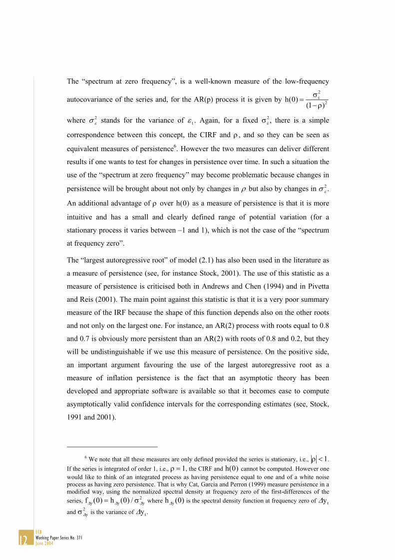
The “spectrum at zero frequency”, is a well-known measure of the low-frequency
autocovariance of the series and, for the AR(p) process it is given by h(
where
)( )
01
2
2=−σρε
σ ε stands for the variance of 2 ε t . Again, for a fixed σε2, there is a simple
correspondence between this concept, the CIRF and ρ , and so they can be seen as
equivalent measures of persistence6. However the two measures can deliver different
results if one wants to test for changes in persistence over time. In such a situation the
use of the “spectrum at zero frequency” may become problematic because changes in
persistence will be brought about not only by changes in ρ but also by changes in σ ε .
An additional advantage of ρ over h( as a measure of persistence is that it is more
intuitive and has a small and clearly defined range of potential variation (for a
stationary process it varies between –1 and 1), which is not the case of the “spectrum
at frequency zero”.
2
)0
The “largest autoregressive root” of model (2.1) has also been used in the literature as
a measure of persistence (see, for instance Stock, 2001). The use of this statistic as a
measure of persistence is criticised both in Andrews and Chen (1994) and in Pivetta
and Reis (2001). The main point against this statistic is that it is a very poor summary
measure of the IRF because the shape of this function depends also on the other roots
and not only on the largest one. For instance, an AR(2) process with roots equal to 0.8
and 0.7 is obviously more persistent than an AR(2) with roots of 0.8 and 0.2, but they
will be undistinguishable if we use this measure of persistence. On the positive side,
an important argument favouring the use of the largest autoregressive root as a
measure of inflation persistence is the fact that an asymptotic theory has been
developed and appropriate software is available so that it becomes ease to compute
asymptotically valid confidence intervals for the corresponding estimates (see, Stock,
1991 and 2001).
6 We note that all these measures are only defined provided the series is stationary, i.e., ρ <1.
If the series is integrated of order 1, i.e., ρ = 1
y∆ ( )0
, the CIRF and h( cannot be computed. However one would like to think of an integrated process as having persistence equal to one and of a white noise process as having zero persistence. That is why Cat, Garcia and Perron (1999) measure persistence in a modified way, using the normalized spectral density at frequency zero of the first-differences of the series, f h where h is the spectral density function at frequency zero of
)0
y y∆ ∆( ) ( ) /0 0 2= y∆σ ∆yt
and σ is the variance of ∆y2 ∆yt .
12
ECBWorking Paper Series No. 371June 2004
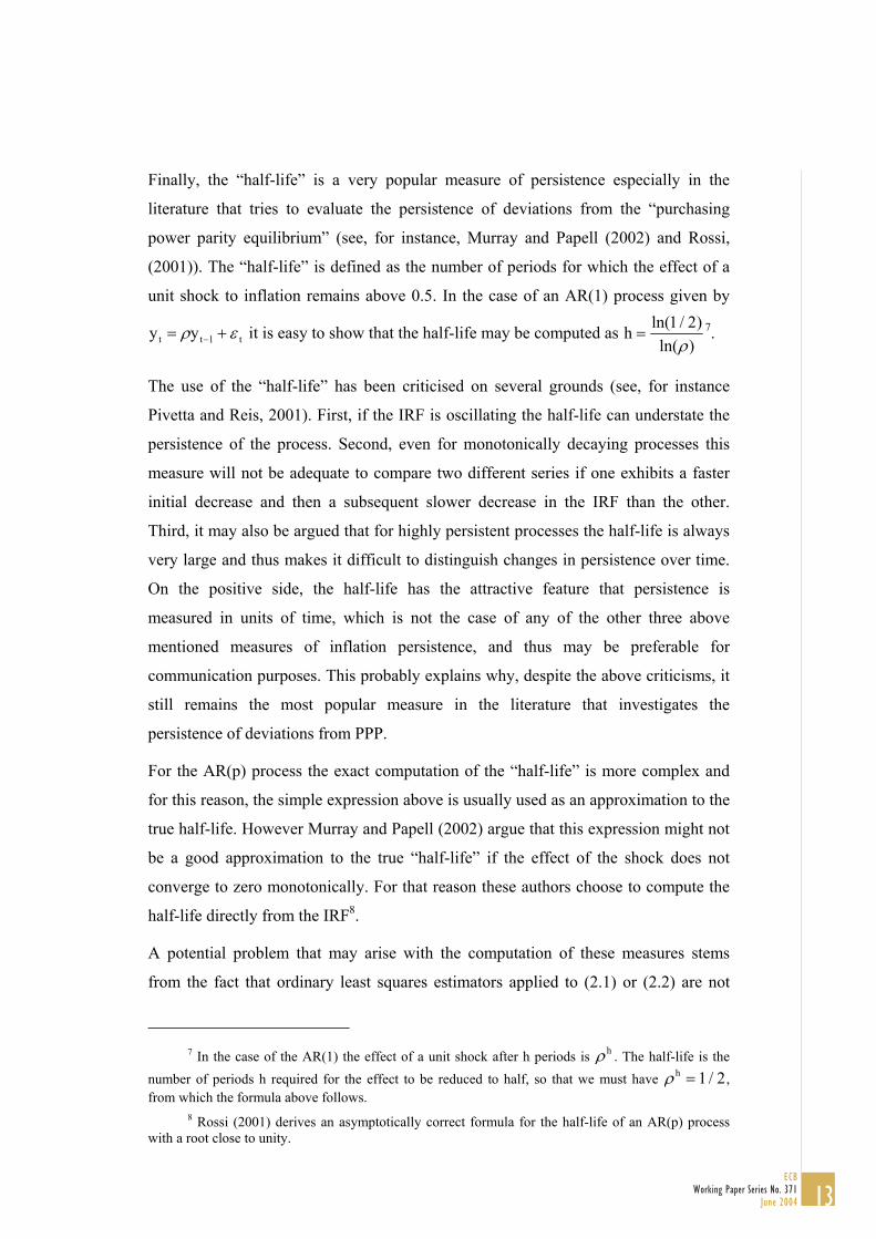
Finally, the “half-life” is a very popular measure of persistence especially in the
literature that tries to evaluate the persistence of deviations from the “purchasing
power parity equilibrium” (see, for instance, Murray and Papell (2002) and Rossi,
(2001)). The “half-life” is defined as the number of periods for which the effect of a
unit shock to inflation remains above 0.5. In the case of an AR(1) process given by
ty yt t= +−ρ ε1 it is easy to show that the half-life may be computed as h =ln( / )ln( )
1 2ρ
7.
The use of the “half-life” has been criticised on several grounds (see, for instance
Pivetta and Reis, 2001). First, if the IRF is oscillating the half-life can understate the
persistence of the process. Second, even for monotonically decaying processes this
measure will not be adequate to compare two different series if one exhibits a faster
initial decrease and then a subsequent slower decrease in the IRF than the other.
Third, it may also be argued that for highly persistent processes the half-life is always
very large and thus makes it difficult to distinguish changes in persistence over time.
On the positive side, the half-life has the attractive feature that persistence is
measured in units of time, which is not the case of any of the other three above
mentioned measures of inflation persistence, and thus may be preferable for
communication purposes. This probably explains why, despite the above criticisms, it
still remains the most popular measure in the literature that investigates the
persistence of deviations from PPP.
For the AR(p) process the exact computation of the “half-life” is more complex and
for this reason, the simple expression above is usually used as an approximation to the
true half-life. However Murray and Papell (2002) argue that this expression might not
be a good approximation to the true “half-life” if the effect of the shock does not
converge to zero monotonically. For that reason these authors choose to compute the
half-life directly from the IRF8.
A potential problem that may arise with the computation of these measures stems
from the fact that ordinary least squares estimators applied to (2.1) or (2.2) are not
7 In the case of the AR(1) the effect of a unit shock after h periods is ρ h . The half-life is the
number of periods h required for the effect to be reduced to half, so that we must have ρ h = 1 2/ , from which the formula above follows.
8 Rossi (2001) derives an asymptotically correct formula for the half-life of an AR(p) process with a root close to unity.
13
ECBWorking Paper Series No. 371
June 2004

free from finite sample biases. To deal with this problem, Andrews and Chen (1994)
developed a “median unbiased estimator”, which is now of widespread use in
empirical applications. This estimation procedure is used not only to obtain median
unbiased estimates but also to compute median unbiased confidence intervals for ρ ,
(see, for instance, Murray and Papell, 2002 and Levin and Piger, 2003).
In summary, from the four measures of persistence just discussed, two of them, the
“sum of autoregressive coefficients “ and the “spectrum at zero frequency” can be
seen as close substitutes as they will tend to deliver the same conclusion for a fixed
sample period. They also appear to be able to deliver the best estimates of inflation
persistence. The “half-life” despite some limitations has the nice property of
delivering persistence in units of time, which can be useful for communication
purposes. In turn, the largest autoregressive root appears as the measure that can
deviate the most from the true persistence of inflation.
In the following sections we focus mainly in ρ , the “sum of the autoregressive
coefficients” as besides being a good measure of inflation persistence it also directly
relates to the mean reversion coefficient of the series, which allows us to propose an
alternative measure of persistence.
3. PERSISTENCE AND MEAN REVERSION
In this section we investigate the close relationship between persistence and mean
reversion. Highlighting such a relationship has some obvious advantages. First, it
allows a deeper understanding of what persistence implies in terms of the time path
for any given stationary time series. Second, helps to emphasise the fact that we
cannot measure persistence without previously addressing the issue of how to measure
the mean of the series. Finally allows us to introduce an alternative simple and
intuitive measure of inflation persistence.
In order to better understand the relationship between persistence and mean reversion
we start by noting that equation (2.2) can be further reparameterised as:
∆ ∆y y yt j t j tj
t
p
= + − −− −=
−
∑δ ρ µ( )[ ]1 11
1
+ ε (3.1)
where
14
ECBWorking Paper Series No. 371June 2004
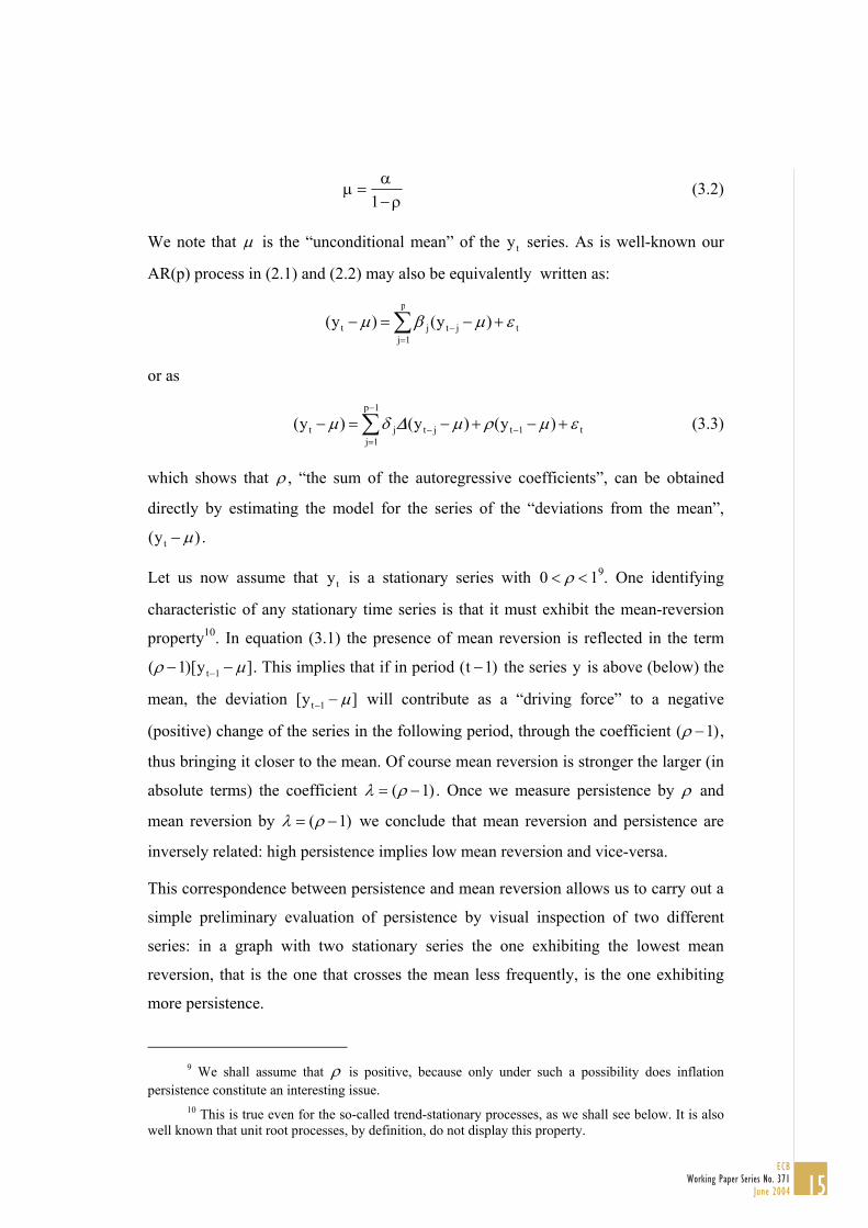
µαρ
=−1
(3.2)
We note that µ is the “unconditional mean” of the series. As is well-known our
AR(p) process in (2.1) and (2.2) may also be equivalently written as:
yt
( ) ( )y yt jj
p
t j− = − +=
−∑µ β µ1
t ε
or as
( ) ( ) ( )y y yt jj
p
t j t t− = − + − +=
−
− −∑µ δ µ ρ µ1
1
1∆ ε (3.3)
which shows that ρ , “the sum of the autoregressive coefficients”, can be obtained
directly by estimating the model for the series of the “deviations from the mean”,
( )yt − µ .
Let us now assume that y is a stationary series with 0t 1< <ρ 9. One identifying
characteristic of any stationary time series is that it must exhibit the mean-reversion
property10. In equation (3.1) the presence of mean reversion is reflected in the term
( )[ ]ρ µ− −−1 1yt . This implies that if in period ( )t −1 the series y is above (below) the
mean, the deviation [ ]yt−1 − µ will contribute as a “driving force” to a negative
(positive) change of the series in the following period, through the coefficient ( )ρ −1 ,
thus bringing it closer to the mean. Of course mean reversion is stronger the larger (in
absolute terms) the coefficient λ ρ= −( 1) . Once we measure persistence by ρ and
mean reversion by λ ρ= −( 1) we conclude that mean reversion and persistence are
inversely related: high persistence implies low mean reversion and vice-versa.
This correspondence between persistence and mean reversion allows us to carry out a
simple preliminary evaluation of persistence by visual inspection of two different
series: in a graph with two stationary series the one exhibiting the lowest mean
reversion, that is the one that crosses the mean less frequently, is the one exhibiting
more persistence.
9 We shall assume that ρ is positive, because only under such a possibility does inflation
persistence constitute an interesting issue. 10 This is true even for the so-called trend-stationary processes, as we shall see below. It is also
well known that unit root processes, by definition, do not display this property.
15
ECBWorking Paper Series No. 371
June 2004
To illustrate how important is the mean for the process of persistence evaluation, let
us assume, for illustrative purposes that y follows a trend stationary process given by t
yt = + +α α ε0 1 (3.4) t t
In the simplest case ε t
t
might be a white noise process, and in this case persistence is
zero. However to get a value of zero for our measures of persistence we need to
properly account for the fact that the series has a time varying mean given by
E yt t[ ] = = +µ α α0 1 . In other words, in order to get a zero value for our measures of
persistence we have to think of the persistence of the white noise series, ε t , that is the
persistence of the deviations from the mean: ε α αt ty t= − −( 0 1 ). Of course, if in
empirical applications, we fail to take due account of the fact that the mean of the
series is time varying and mistakenly assume it as constant over time, we are bound to
conclude that the series is highly persistent when in fact it has no persistence at all. In
general, for an assumed constant mean, any change in level of inflation will show up
as higher persistence. On the contrary, a time varying mean will imply lower
persistence (higher mean reversion), other things equal. In the limit, by assuming a
constant mean we can turn a zero persistence series into a highly persistent one, or the
other way round, by assuming a very flexible mean for inflation.
Some literature has to some extent recognized the liaison between persistence and the
way the mean of the series is treated, and has tried to deal with the problem by
identifying some “structural breaks in the level” of the series (see for instance
Burdekin and Syklos (1999), Bleaney (2001), and Levin and Piger, (2003)). For
instance, Levin and Piger (2003) investigate inflation persistence for 12 countries and
4 measures of inflation, in the period 1984-200211. In a first step the analysis is
conducted under the assumption of a constant mean of the series for the whole period
and the general conclusion is that inflation appears to be highly persistent, in most
cases. In a second step the authors allow for the possibility of a structural break in the
mean of the series and the general conclusion changes dramatically, the new global
picture being one of low inflation persistence. Moreover, the reduction in estimated
persistence is especially large for the countries for which the evidence of a structural
11 The countries analysed are: Australia, Canada, France, Germany, Italy, Japan, The Netherlands, New Zealand, Sweden, Switzerland, United Kingdom and United States. For each country four diferent measures of inflation are investigated: GDP deflator, CPI, Core CPI and PCE deflator.
16
ECBWorking Paper Series No. 371June 2004
break is stronger12. Countries for which evidence of a structural break is weaker are
also the ones where remaining inflation persistence is higher13 (even though the
evidence changes somewhat according to inflation measures). However, a natural
remaining question regarding the work by Levin and Piger is whether the higher
persistence found for these latter countries is a real feature of the data or rather a
spurious result brought about by the assumption of a constant mean with a single
break during the sample period. At least for some countries, allowing for a time
varying mean appears as a reasonable alternative that may significantly change the
conclusions about persistence.
In our opinion investigating inflation persistence under the univariate approach
requires much more than simply accounting for the possibility of some potential
discrete structural breaks in the mean of the series. In fact, it is unclear why one
should test for breaks in the intercept when evaluating persistence. Testing for breaks
in the intercept appears as a natural way to proceed in the context of the unit root
literature. In such a context, we may whish to decide whether the data are better
described by a model with a single intercept or by a model with two or more different
intercepts. This of course also may have important consequences for the estimated
persistence (the ρ parameter). However, in the context of persistence evaluation it is
unclear why we should expect the second model to deliver a better estimate of
persistence, as there is no reason why we should expect the mean which underlies the
model with breaks in the intercept to be a better proxy for the unknown “long run
level of inflation”14.
Given that, under the univariate times series representation of inflation, the mean of
inflation is the level to which inflation returns after a shock, we see the mean of the
series as playing the role of the long run level of inflation, the importance of which
was discussed in the previous section. Thus, unless we have a theory or a model that
allow us to reasonably assume that the long run equilibrium level of inflation can be
12 These are: Australia, Canada, Italy, Sweden, The United Kingdom and the United States. 13 These are: France, Netherlands, New Zealand, Germany, Japan and Switzerland. 14 Moreover, it can be argued that testing for breaks implies endogeneising the mean because the
outcome of such tests is conditional on a given estimated model. In other words, rather than computing persistence conditional on a given exogenous mean, as seems the natural thing to do given the exogeneity of the central inflation target, this approach computes the mean conditional on (or simultaneously with) the estimated persistence.
17
ECBWorking Paper Series No. 371
June 2004
treated as a constant over the period under investigation, it seems more natural to
assume a time varying mean, as the null hypothesis. Of course, under such a
framework, the question of how to deal with an exogenous time varying mean
naturally follows.
One can argue that without a theoretical model for the long run level of inflation we
cannot expect to give the univariate approach a meaningful interpretation. However,
specifying a theoretical model for the long run level of inflation will drive us away
from the univariate framework into the multivariate approach. Thus, in order to stay
within the univariate approach, we must use a pure statistical model to extract the
mean of inflation. In this regard, the Hodrik-Prescott (HP) filter, the Baxter and King
“band-pass filter” or simple “centred moving averages” appear as obvious candidates.
We can also think of alternative measures of core inflation, provided these meet some
required statistical criteria, as the ones suggested in Marques et al. (2002 and 2003).
But of course by following such a an approach one is assuming that no matter what
the truelong run driving forces of inflation are, the “long run level” of inflation can be
well approximated by such statistical devices. For countries in which a credible
inflation-targeting monetary policy has been followed we can also use the
“exogenously announced inflation target” and for countries, where they are available,
survey inflation-expectations can also be used15.
In concluding this section, we may summarize the above discussion in two main
points. First, when evaluating the persistence of the series what really matters is the
persistence of deviations from the mean. Second, we should not address inflation
persistence without a previous discussion of how we expect the mean of the series,
i.e., the “long run level” of inflation to have evolved over time, as failure to properly
account for changes in the mean of the series will show up as (spurious) higher
persistence.
15 See, for instance, Kozicki and Tinsley (2003) or Kieler (2003)).
18
ECBWorking Paper Series No. 371June 2004

4. AN ALTERNATIVE MEASURE OF PERSISTENCE
Given the monotonic relationship between the “sum of the autoregressive
coefficients” (ρ) and the coefficient of mean reversion (λ ) it appears natural to define
the ratio
γ = −1 nT
(4.1)
as a measure of inflation persistence, where n stands for the number of times the
series crosses the mean during a time interval with T+1 observations.
The γ statistic has the advantage of not requiring the researcher to specify and
estimate a model for the inflation process. For this reason it can be expected to be a
robust statistic against model misspecifications.
We note that γ , by construction, is always between zero and one. However, it can be
shown (see Appendix A) that for a symmetric zero mean white noise process we have
E γ = 0 5. , so that values of γ close to 0.5 signal the absence of any significant
persistence (white noise behaviour) while figures significantly above 0.5 signal
significant persistence. On the other hand, figures below 0.5 signal a negative ρ , that
is, negative long-run autocorrelation. It is also shown in Appendix A that under the
assumption of a symmetric white noise process for inflation (zero persistence) the
following result holds:
γ −∩
0 50 5
0 1.. /
& ( ; )T
N (4.2)
Result (4.2) allows us to carry out some simple tests on the statistical significance of
the estimated persistence (i.e., γ =0.5)16. We note however that result (4.2) is valid
only under the assumption of a pure white noise process and that if the null of γ =0.5
is rejected, we should expect γ to have a more complicated distribution, which, in
particular, may depend on the characteristics of the data generating process.
An additional interesting property of γ is that there is a simple relation between the
estimate of γ for a given period with T+1 observations and the estimated γ ’s for two
16 For instance for a sample with T=100 the null of γ =0.5 (zero persistence) will be rejected for
any estimated γ larger than 0.60.
19
ECBWorking Paper Series No. 371
June 2004
non-overlapping consecutive sub-periods with T +1 and T +1 observations such that
T+1= (T +1)+(T +1). In fact we have 1 2
1 2
2
2
− =γ α
)
t j
(j )t j +
−µ
1 11 2
1 2
1
1
1
1 2
2
1 21 2≈
++
=+
++
= − + − −nT
n nT T
nT
TT T
nT
TT T
( ) ( )( 1 1γ α γ )
or simply
γ αγ α γ≈ + −1 1( (4.3) 2
t
so that persistence for the whole period is (approximately) a weighted average of the
persistence for the two consecutive periods.
Below we will consider the possibility of a pure time varying mean for inflation. In
such case we measure persistence of the deviations from the time varying mean and
our model may be written as
y yt t jj
p
= + +−=∑α β
1
ε (4.4)
or equivalently as
( )y yt tj
p
t j t− = −=
− −∑µ β µ1
(4.5) ε
or further as
( ) ( ) ( )y y yt t jj
p
t j t j t t− = − + − +=
− − −∑µ δ µ ρ1
1 1∆ t (4.6) ε
which corresponds to the general model used in section 5.
5. PERSISTENCE AND MEAN REVERSION: RE-EVALUATING
INFLATION PERSISTENCE IN THE UNITED STATES AND THE
EURO AREA
In this section we illustrate the issues discussed above, by re-evaluating the evidence
on inflation persistence for the United States (U.S.) and the Euro Area (E.A.). For the
U.S. both the GDP deflator and the consumer price index are analysed while for the
Euro Area, for reasons of data availability, only the consumer price index is
20
ECBWorking Paper Series No. 371June 2004

investigated17. For reasons of space the analysis will mainly focus on the U.S. GDP
deflator, so that results on the consumer price indices for the U.S. and E.A. are only
explicitly mentioned when they are thought to add to the conclusions. However, all
the results for the three series are equally presented in Appendix B. As measures of
persistence we mainly use ρ , the “sum of the autoregressive coefficients” and γ the
“the proportion of mean crossings”, suggested in the previous section.
There is now a widely accepted view in the literature that inflation has been more
persistent during the sixties and seventies than thereafter. For instance, Levin and
Piger (2003) write, “there is widespread agreement that inflation persistence was very
high over the period extending from 1965 to the disinflation of the early 1980s.
However, there is substantial debate regarding whether inflation persistence continued
to be high since the early 1980s, or has declined”. In the same vein see Cogley and
Sargent (2001), Willis (2003) and Guerrieri (2002)18.
Graph No.1 displays quarterly inflation in the U.S. as from 1960q2 to 2002q4 using
the GDP deflator. This series has been analysed among others by Taylor (2000),
Cogley and Sargent (2001), Pivetta and Reis (2001) and Levin and Piger (2003).
Let us start by focussing on the mean of inflation. Simple visual inspection of Graph
No.1 suggests that we can basically distinguish three distinct periods. The first period
stretches from the beginning of the sample until roughly the end of 1980. During this
period, inflation exhibits a clear upward trend. Thus, if anything, the data suggest that
we should not embark in a persistence evaluation exercise without accounting for the
possibility of a time varying mean. Clearly assuming a constant mean as has been
done in some literature does not appear a realistic approach.
17 For the Euro Area the official data on the GDP price deflator are available only after 1992q1,
which motivated not including this series in the analysis. Also the aggregate consumer price index for the twelve countries of the euro area only starts in 1967q1, which conditioned the final sample period used in the analysis. The original data for the consumer price index in the U.S. refers to the series of “consumer prices, all items, all urban consumers, seasonally adjusted” for the period 1967q1 to 2002q4 (IMF series) while the series for the Euro Area corresponds to the original 12 euro area countries (with fixed weights), for the same period. In turn, the original data for the quarterly GDP price deflator were downloaded from the Bureau of Economic Analysis website and refers to a somewhat longer period (1960q1 to 2002q4), in order to allow comparability with other empirical studies. In all cases, the inflation rate is obtained as the first difference of logged price indices.
18 Against this view see, however, Pivetta and Reis (2001) and Stock (2001). These authors argue that there is not enough evidence to conclude for a change in persistence.
21
ECBWorking Paper Series No. 371
June 2004
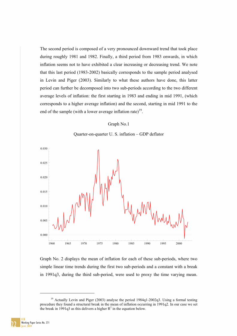
The second period is composed of a very pronounced downward trend that took place
during roughly 1981 and 1982. Finally, a third period from 1983 onwards, in which
inflation seems not to have exhibited a clear increasing or decreasing trend. We note
that this last period (1983-2002) basically corresponds to the sample period analysed
in Levin and Piger (2003). Similarly to what these authors have done, this latter
period can further be decomposed into two sub-periods according to the two different
average levels of inflation: the first starting in 1983 and ending in mid 1991, (which
corresponds to a higher average inflation) and the second, starting in mid 1991 to the
end of the sample (with a lower average inflation rate)19.
Graph No.1
Quarter-on-quarter U. S. inflation – GDP deflator
1960 1965 1970 1975 1980 1985 1990 1995 2000
0.000
0.005
0.010
0.015
0.020
0.025
0.030
Graph No. 2 displays the mean of inflation for each of these sub-periods, where two
simple linear time trends during the first two sub-periods and a constant with a break
in 1991q3, during the third sub-period, were used to proxy the time varying mean.
19 Actually Levin and Piger (2003) analyse the period 1984q1-2002q3. Using a formal testing
procedure they found a structural break in the mean of inflation occurring in 1991q2. In our case we set the break in 1991q3 as this delivers a higher R2 in the equation below.
22
ECBWorking Paper Series No. 371June 2004

Specifically the mean of inflation in Graph No.2 is obtained as the fitted values of the
regression model:
π t t d t d d= + + − + −
− −
0 0008 0 0003 0 1792 0 0018 0 0075 0 0036130 19 5 5 4 99 915 5
1 2 2 3. . . . . .( . ) ( . ) ( .43) ( . ) ( . ) ( .44)
4
estimated for the period 1960q2 to 2002q420. The lower panel of Graph No.2 displays
the residuals of the regression, i.e., the deviations from the mean of inflation. A
similar decomposition for the consumer price indices in the U.S. and the E.A. is
performed in Appendix B (see Graphs B.3 and B.8)21.
Graph No.2
Quarter-on-quarter U. S. inflation – GDP deflator
1960 1965 1970 1975 1980 1985 1990 1995 2000
0.00
0.01
0.02
0.03
INFLATION AND MEAN OF INFLATION
1960 1965 1970 1975 1980 1985 1990 1995 2000
-2.5
0.0
2.5
5.0
DEVIATIONS FROM THE MEAN
Some of the analyses carried out for the U.S. as regards how the mean of inflation is
treated, can be seen as special cases of Graph No.2. For instance, Taylor (2000)
20 The variables are defined as follows: t = time trend for the period 1960q2 to 1980q4; t =
time trend for the period 1981q1 to 1983q1;1 2
d2 = constant for the period 1981q1 to 1983q1; d3 = constant for the period 1983q2 to 2002q4; d4 = constant for the period 1991q3 to 2002q4. As expected this static regression exhibits some autocorrelation. However all the coefficients remain significant (except the global constant) when we allow for six lags of inflation to account for serial correlation. This can be seen as evidence that the assumed (deterministic) time profile for the mean in Graph No.2 is consistent with the data.
21 We note that the specific dates used to define the different sub-periods for each series where identified after eyeballing the series and are such that the resulting mean fits the data in the smoothest possible way.
23
ECBWorking Paper Series No. 371
June 2004
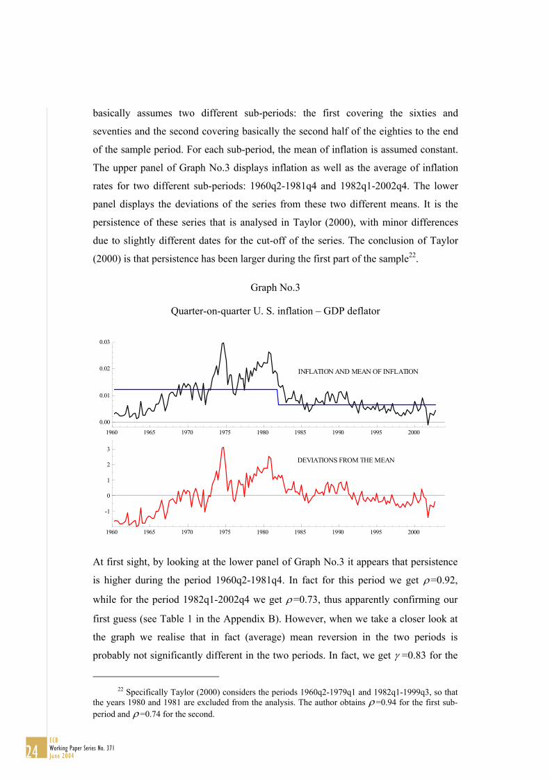
basically assumes two different sub-periods: the first covering the sixties and
seventies and the second covering basically the second half of the eighties to the end
of the sample period. For each sub-period, the mean of inflation is assumed constant.
The upper panel of Graph No.3 displays inflation as well as the average of inflation
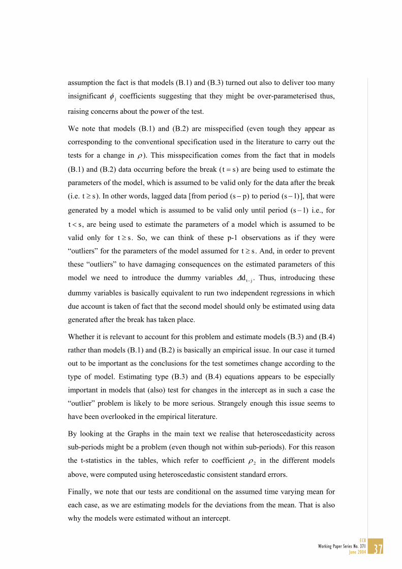
rates for two different sub-periods: 1960q2-1981q4 and 1982q1-2002q4. The lower
panel displays the deviations of the series from these two different means. It is the
persistence of these series that is analysed in Taylor (2000), with minor differences
due to slightly different dates for the cut-off of the series. The conclusion of Taylor
(2000) is that persistence has been larger during the first part of the sample22.
Graph No.3
Quarter-on-quarter U. S. inflation – GDP deflator
1960 1965 1970 1975 1980 1985 1990 1995 2000
0.00
0.01
0.02
0.03
INFLATION AND MEAN OF INFLATION
1960 1965 1970 1975 1980 1985 1990 1995 2000
-1
0
1
2
3
DEVIATIONS FROM THE MEAN
At first sight, by looking at the lower panel of Graph No.3 it appears that persistence
is higher during the period 1960q2-1981q4. In fact for this period we get ρ=0.92,
while for the period 1982q1-2002q4 we get ρ=0.73, thus apparently confirming our
first guess (see Table 1 in the Appendix B). However, when we take a closer look at
the graph we realise that in fact (average) mean reversion in the two periods is
probably not significantly different in the two periods. In fact, we get γ =0.83 for the
22 Specifically Taylor (2000) considers the periods 1960q2-1979q1 and 1982q1-1999q3, so that
the years 1980 and 1981 are excluded from the analysis. The author obtains ρ=0.94 for the first sub-period and ρ=0.74 for the second.
24
ECBWorking Paper Series No. 371June 2004
first sub-period and γ =0.80 for the second sub-period (γ =0.81 for the whole period)
suggesting that there may not be a strong evidence of a change in persistence23.
In formal terms we tested the change in persistence by estimating models (B.1) to
(B.4) which are described in Appendix B. According to model (B.1) and (B.3) we
would conclude that there is not a strong evidence favouring the idea of a significant
change in persistence between the two periods (see Table 1 in Appendix B). However
the conclusion is reversed if we rather retain the results of models (B.2) and (B.4).
According to these models, which are not likely to suffer from over-parameterisation
and thus allow more efficient inference the null of equal ρ s for the two sub-periods
can be rejected24.
A similar conclusion can be drawn for the consumer price index in the U.S. even
though the evidence of a change in persistence between the two sub-periods is not as
strong as in the case of the GDP deflator. However, for the E.A., even though the
point estimates of ρ and γ suggest that we still are in the presence of a significantly
persistent process (we get ρ=0.85 and γ =0.79 for the sub-period 1967/2-1983/4 and
ρ=0.80 and γ =0.74 for the sub-period 1984/1-2002/4) there is no evidence of a
significant decline between these two sub-periods (see Graphs B.1 and B.6 and Table
1 in Appendix B for details). So, from the situation depicted in Graph No.3 (and
similarly in Graphs B.1 and B.6), which basically corresponds to the conventional
analysis carried out in the literature that assumes a constant mean in each sub-period,
we conclude that 1) inflation in the U.S. and the E.A. appears to have been highly
persistent in the sixties and seventies (first sub-period) 2) inflation persistence in the
23 We note that we do not have a test statistic to formally discuss whether the two estimates of
γ are statistically different or not, so that strictly speaking, we cannot be sure whether these two magnitudes are statistically equivalent.
A potential explanation for the fact that the estimated ρ s differ a lot between the two periods while γ does not is that the estimated ρ in the first period is probably biased upwards due to the fact that mean reversion rather than being spread out all over the sample period is highly concentrated in the middle of the period (1968-1972). This also suggests that, if we assume a constant mean, then the period 1960-1981 is not homogenous in what regards inflation persistence. In terms of mean reversion we can distinguish three different sub-periods in Graph No.3: a first sub-period that goes from the beginning of sample (1960) until 1967 in which there is no mean reversion at all; a second sub-period in which mean reversion is high (1968-1973) and again a sub-period with very high persistence (1973-1981).
24 We note that the structural break tests conducted in Appendix B correspond to the classical Chow tests, in which the break date is assumed to be fixed and known, rather than allowing for a break at an unknown date as in the methodology developed by Andrews (1993).
25
ECBWorking Paper Series No. 371
June 2004
U.S has declined during the last twenty years or so (second sub-period) and 3) there is
not a strong evidence that inflation persistence in the E.A has declined during the last
two decades or so.
The previous approach to persistence evaluation has as its main limitation the fact that
it assumes a constant mean for inflation during each sub-period. Most likely, many
econometricians would argue that during the first sub-period (1960-1981), rather than
exhibiting mean reversion, the GDP inflation series in Graph No.3 is more likely to be
non-stationary. In fact an ADF test for this period (assuming a constant mean) reveals
that the null of a unit root cannot be rejected casting strong doubts on the usefulness
of measuring inflation persistence for the U.S. during this period assuming a constant
mean25. Of course, the above test on the statistical significance for the difference in
the estimated ρ s is not valid if the series is not stationary.
To see how things can change let us now assume that the mean of inflation during the
first two sub-periods (1960q2-1980q4 and 1981q1-1983q1) may be approximated by
two linear time trends as in Graph No.2. This new possibility is displayed in Graph
No.4 (upper panel), which differs from Graph No.2 in that it assumes a constant mean
with no break for the whole sub-period 1983q2-2002q4. The ADF unit root test
suggests that assuming a linear time trend to measure the mean of inflation in the sub-
period 1960q2 to 1980q4 is a reasonable alternative (statistically speaking), as in such
case, the null of a unit root is rejected in favour of a trend stationary process for
inflation.
Now we have a different picture. Looking at the lower panel of Graph No.4, it is no
longer so obvious that persistence for the period 1960-1980 has been higher than
persistence in the period 1981- 2002. In fact, if anything, the results are now the other
way round. First, for the whole period we now get ρ=0.58 and γ =0.70 suggesting the
absence of any significant persistence. Second, we get estimates of persistence for the
first sub-period which are lower (though not significantly so) than the ones for the
second sub-period, in contrast with the previous situation. In fact, for the sub-period
1960q2-1980q4 we now have ρ=0.45 and γ =0.66 while for the sub-period 1981q1-
2002q4 we have ρ=0.79 and γ =0.74. Thus, once we allow for a time varying mean
25 The ADF test for the U.S. GDP deflator can be computed from Table 1 as (0.92-1)/0.052= -
1.53, so that the null of a unit root in inflation for the sub-period 1960q2-1981q4 cannot be rejected even for a 10% test.
26
ECBWorking Paper Series No. 371June 2004
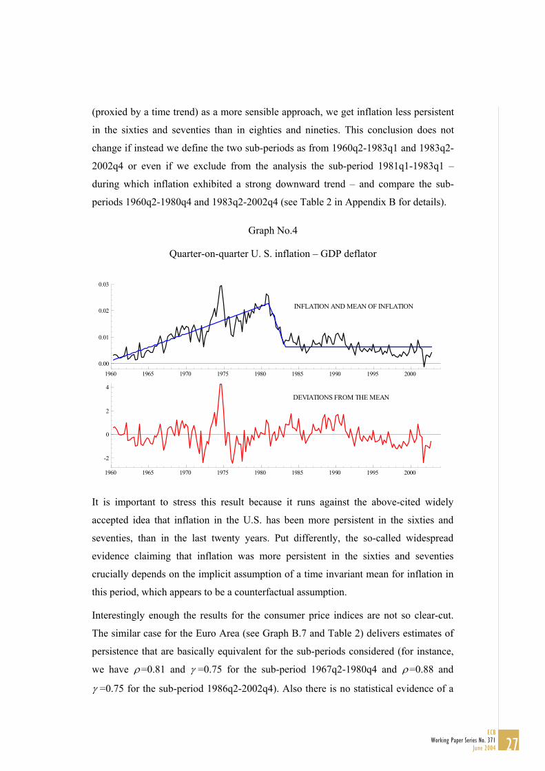
(proxied by a time trend) as a more sensible approach, we get inflation less persistent
in the sixties and seventies than in eighties and nineties. This conclusion does not
change if instead we define the two sub-periods as from 1960q2-1983q1 and 1983q2-
2002q4 or even if we exclude from the analysis the sub-period 1981q1-1983q1 –
during which inflation exhibited a strong downward trend – and compare the sub-
periods 1960q2-1980q4 and 1983q2-2002q4 (see Table 2 in Appendix B for details).
Graph No.4
Quarter-on-quarter U. S. inflation – GDP deflator
1960 1965 1970 1975 1980 1985 1990 1995 2000
0.00
0.01
0.02
0.03
INFLATION AND MEAN OF INFLATION
1960 1965 1970 1975 1980 1985 1990 1995 2000
-2
0
2
4
DEVIATIONS FROM THE MEAN
It is important to stress this result because it runs against the above-cited widely
accepted idea that inflation in the U.S. has been more persistent in the sixties and
seventies, than in the last twenty years. Put differently, the so-called widespread
evidence claiming that inflation was more persistent in the sixties and seventies
crucially depends on the implicit assumption of a time invariant mean for inflation in
this period, which appears to be a counterfactual assumption.
Interestingly enough the results for the consumer price indices are not so clear-cut.
The similar case for the Euro Area (see Graph B.7 and Table 2) delivers estimates of
persistence that are basically equivalent for the sub-periods considered (for instance,
we have ρ=0.81 and γ =0.75 for the sub-period 1967q2-1980q4 and ρ=0.88 and
γ =0.75 for the sub-period 1986q2-2002q4). Also there is no statistical evidence of a
27
ECBWorking Paper Series No. 371
June 2004

change in persistence between the two sub-periods. However for the U.S. consumer
price index the conclusion very much depends on the sub-periods considered. If we
compare the sub-periods 1967q2-1980q2 and 1980q3-2002q4 we conclude (using
models B.2 and B.4) that persistence is higher during the first sub-period. However, if
we rather take the two sub-periods 1967q2-1982q4 and 1983q1-2002q4 we get no
evidence of a change in persistence. The reason for such a different conclusion stems
from the effect of the sub-period 1980q3-1982q4 during which the estimated
persistence is very low. If we exclude this sub-period from the analysis we conclude
that persistence during the sub-period 1967q2-1980q4 and 1983q1-2002q4 is basically
the same when measured by ρ .
Of course this is not the end of the story since by looking at the inflation series we can
think of many other reasonable possibilities to measure the mean of inflation. For
instance, if we now also assume two different means for the sub-period 1983-2002, as
in Levin and Piger (2003) we end up with the situation described in Graph No.2, with
the residuals (deviations from the mean) depicted in the corresponding lower panel.
Now again we have a different picture. For the U.S. GDP deflator we get estimates for
ρ which display an impressive constancy (see Table 3 in Appendix B). For the all the
sub-periods considered we have ρ=0.45 and thus the idea we get from the analysis of
Graph No.2 is that the persistent process has now evaporated. This conclusion is to
some extent confirmed by the statistics γ (which varies between 0.60 and 0.66)26.
The results of a similar treatment for the consumer price indices in the U.S. and the
E.A. can be seen in Graphs B.3 and B.8. and Table 3 in Appendix B. For the U.S.
allowing for a break in the mean during the last sub-period (1983q1-2002q4) does not
change the results in any significant way (vis-à-vis the previous situation). In
particular the γ statistic does not change at all. The reason is that in contrast to the
GDP series there seems to be no significant evidence of a break in the mean of the
U.S. CPI inflation (compare Graphs B.2 and B.3). For the E.A. allowing for a break in
the mean during the last sub-period reduces the estimates of persistence for this sub-
period (as well as for the whole period), as expected. Now there is some (weak)
evidence of a change in persistence when we compare the sub-periods 1967q2-1980q4
26 We note that ρ=0.50 implies a half-life equal to 1 and thus absence of a significant
persistence. Also it is easy to see that γ =0.60 is close to being not significantly different from 0.50 (zero persistence).
28
ECBWorking Paper Series No. 371June 2004

and 1981q1-2002q4 (model B.2) even though such evidence does not stand when we
compare the sub-periods 1967q2-1986q1 and 1986q2-2002q4.
Of course, one may argue that there are no theoretical reasons why the mean of
inflation should evolve over time as assumed in Graph No.2. A less subjective
solution (in the sense that it is not defined after looking at the data) can be obtained by
entertaining the possibility of a pure time varying mean and see what happens to
inflation persistence under such circumstances. We consider two different possibilities
for the mean of inflation: the widely used HP filter (with λ=1600) which is depicted
in Graph No. 5 and the 13 terms centred moving average, which is displayed in Chart
No.6. We note that the “moving average mean” is more flexible than the “HP mean”
and that this will show up in lower persistence estimates.
Graph No.5
Quarter-on-quarter U. S. inflation – GDP deflator
1960 1965 1970 1975 1980 1985 1990 1995 2000
0.00
0.01
0.02
0.03
INFLATION AND MEAN OF INFLATION
1960 1965 1970 1975 1980 1985 1990 1995 2000
-0.005
0.000
0.005
0.010DEVIATIONS FROM THE MEAN
Now we see that while there seems to be still some residual (even though not
significant) inflation persistence under the “HP mean” (we get ρ=0.44 and γ =0.60
for the U.S. GDP deflator), the “moving average mean” has basically removed all the
persistence in the inflation series (we have ρ=-0.03 and γ =0.52). Moreover, once
again there seems to be no strong evidence of a difference in persistence for the two
29
ECBWorking Paper Series No. 371
June 2004

periods under analysis, i.e., there seems to be no change in inflation persistence
through time. These conjectures are formally tested and confirmed in Tables 4 and 5.
These conclusions also stand for the consumer price indices in the U.S and the E.A.
(see Graphs B.4 and B.5 for the U.S. and Graphs B.9 and B.10 for the E.A. and Tables
4 and 5)27.
Graph No.6
Quarter-on-quarter U. S. inflation – GDP deflator
1960 1965 1970 1975 1980 1985 1990 1995 2000
0.00
0.01
0.02
0.03
INFLATION AND MEAN OF INFLATION
1960 1965 1970 1975 1980 1985 1990 1995 2000
-0.005
0.000
0.005
0.010
DEVIATIONS FROM THE MEAN
A noteworthy final remark regards the use of ρ as a measure of inflation persistence.
In several cases the estimates for ρ turn out to be very sensitive to the number of lags
of the selected model. For instance, in Table 3 the estimate ρ=0.45 for the U.S: GDP
deflator during the sub-periods 1981q1-2002q4 or 1983q2-2002q4 is obtained for a
model with three lags28. However if a model with a single lag were chosen, we would
get ρ=0.25 for the period 1981q1-2002q4 and ρ=0.30 for the sub-period 1983q2-
27 As regards the U.S CPI we can see from Tables 4 and 5 that there seems to be some evidence
of a decrease in persistence when we compare the periods (1967q2-1980q2) with the period (1980q3-2002q4), but once again such evidence disappears when we compare the period (1967q2-1982q4) with the period (1983q1-2002q4). The important point however is that the estimates of persistence for any sub-period are not statistically different from zero (i.e., γ is not statistically different from 0.5 or ρ is such that the implied half-life is less than 1).
28 Such cases are marked ** in Tables 1 to 5 in Appendix B.
30
ECBWorking Paper Series No. 371June 2004

2002q4. In such cases γ may be seen as an interesting alternative measure of
persistence as it does not require specifying an estimating a model to inflation.
Summing up, this section shows that the evidence on inflation persistence
dramatically changes with the assumption on the mean of inflation. In particular, the
evidence on whether inflation persistence was higher in the sixties and seventies than
in the two last decades or whether inflation is persistent at all, ultimately hinges on the
type of mean assumed when computing persistence. This section considers some
statistical approaches to proxy the (time varying) mean of inflation, but, of course,
other alternatives, as the ones discussed in section 3, could have been entertained.
However, the real issue is that the reliability of any estimate of inflation persistence
ultimately depends on how realistic the assumed long run inflation path is.
6. CONCLUSIONS
The main conclusions of this paper, which addresses some inflation persistence issues
in the context of the univariate approach, may be summarized as follows.
First, it is stressed that any estimate of inflation persistence is conditional on a given
assumption for the long run equilibrium level of inflation, which in the context of the
univariate approach is proxied by the mean of inflation. Moreover, it is seen that there
is a trade off between persistence and flexibility of the assumed long run level of
inflation. In particular, persistence is maximised by assuming a time invariant mean
for inflation.
Second, it is argued that the commonly followed empirical approach of computing
inflation persistence under the assumption of a constant mean or of a piecewise
constant mean, i.e., allowing for some structural breaks in the intercept of the
estimated model, does not constitute a promising way to deal with the problem.
Third, exploring the relationship between persistence and mean reversion an
alternative statistic to measure inflation persistence is suggested, which has the
advantage of not requiring specifying and estimating a model for inflation.
Finally, estimates of inflation persistence for the U.S. and the Euro Area using
quarterly GDP deflator and CPI are computed. Several sub-periods as well as different
ways of proxying a time varying mean are considered. From this exercise a major
31
ECBWorking Paper Series No. 371
June 2004

conclusion emerges: the evidence on whether inflation persistence was higher in the
sixties and seventies than in the two last decades or whether inflation is persistent at
all, ultimately hinges on the type of mean assumed when computing persistence.
The crucial dependence of the results on the assumed long run level of inflation
obviously puts into question the usefulness of the univariate approach to investigate
inflation persistence, unless we can find an acceptable proxy for the time varying
mean of inflation. For countries for which a credible inflation-targeting monetary
policy has been implemented using the exogenously announced inflation target to
proxy the mean of inflation seems to be the natural solution. However, a problem
remains for countries (or sample periods) for which it is not reasonable to assume a
constant inflation target (for instance, most European countries in the sixties and the
seventies or even in the nineties during the convergence period, before the launching
of the euro). For such cases, before we are able to draw robust conclusions on
inflation persistence, in the context of the univariate analysis, more work needs to be
done in order to identify reliable measures for the long run level of inflation. A way
out could be for researchers to agree on a small number of ways to compute a
(potentially) time varying mean. This will allow obtaining comparable estimates for
different countries and for different time periods.
REFERENCES
Andrews, D.W.K., 1993, “Tests for parameter instability and structural change with
unknown change point”, Econometrica, 61, 821-856;
Andrews, D.W.K., Chen H-Y, 1994, “Approximately median-unbiased estimation of
autoregressive models”, Journal of Business & Economic Statistics, Vol.12,
No.2, 187-204;
Batini, N., 2002, “Euro area inflation persistence”, ECB, WP. No.201;
Batini, N., Nelson, E., 2002, “The lag from monetary policy actions to inflation:
Friedman revisited”, Bank of England, Discussion Paper No.6;
Bleaney, M., 2001, “Exchange rate regimes and inflation persistence”, IMF Staff
Papers, Vol. 47, No.3;
32
ECBWorking Paper Series No. 371June 2004
Burdekin R.C.K., Syklos P.L., 1999, ”Exchange rate regimes and shifts in inflation
persistence: does nothing else matter?, Journal of Money, Credit, and
Banking, Vol. 31, No.2, 235-247;
Cati R.C., Garcia M.G.P., Perron P., 1999, “Unit roots in the presence of abrupt
governmental intervention with an application to brazilian data”, Journal of
Applied Econometrics, 14, 27-56;
Cogley T., Sargent, T., 2001, “Evolving post-war II U.S. inflation dynamics”, NBER,
Macroeconomics Annual edited by Ben S. Bernanke and Kenneth Rogoff;
Guerrieri, L., 2002, “The inflation persistence of staggered contracts”, Board of
Governors of the Federal Reserve System;
Kieler, M., 2003, “Is inflation higher in the euro area than in the United States?”, IMF
country Report No.03/298;
Kozicki, S., Tinsley, P.A., 2002, “Alternative sources of the lag dynamics of
inflation”, RWP 02-12, Federal Reserve Bank of Kansas City;
Levin A. T., Piger J. M., 2003, “Is inflation persistence intrinsic in industrial
economies”? mimeo
Marques C., R., Neves, P. D., Silva, A.G., 2002, “Why should central banks avoid the
use of the underlying inflation indicator?”, Economics Letters, Vol. 75, 17-
23;
Marques C., R., Neves, P. D., Sarmento L.M., 2003, “Evaluating core inflation
indicators”, Economic Modelling, Vol.20/4, 765-775;
Murray C. J., and Papell D. H., 2002, “The purchasing power parity persistence
paradigm”, Journal of International Economics, 56, 1-19;
Pivetta F., Reis, R., 2002, “The persistence of inflation in the United States”, mimeo;
Rossi B., 2001, “Confidence intervals for half-life deviations from purchasing power
parity”, mimeo;
Stock, J., 1991, “Confidence intervals for the largest autoregressive root in the US
macroeconomic time series”. Journal of Monetary Economics, 28, 435-459;
Stock, J., 2001, “Comment”, NBER, Macroeconomics Annual, edited by Ben S.
Bernanke and Kenneth Rogoff;
Taylor, J.B., 2000, “Low inflation, pass-through, and the pricing power of firms”,
European Economic Review, 44, 1389-1408;
33
ECBWorking Paper Series No. 371
June 2004
Willis, J., L., 2003, “Implications of structural changes in the U.S. economy for
pricing behavior and inflation dynamics”, Economic Review, First Quarter
2003, Federal Reserve Bank of Kansas City;
34
ECBWorking Paper Series No. 371June 2004

APPENDIX A – PERFORMING STATISTICAL TESTS ON THE γ STATSISTIC
In this appendix we derive equations (4.2), which allows us to carry out the test of
γ =0.5.
Derivation of equation (4.2)
Let ε stand for a zero mean white noise process, such that t ε t will assume positive and
negative values with equal probability, and define x as a random variable such that
=1 if the series crosses the mean, i.e., if
t
xt ε εt t. −1<0 and x =0 if t ε εt t. −1>0. Then our
measure of persistence can be written as
γ = − = −∑11
x T xt
T
/ 1 (A.1)
where x is a random variable with a Bernoulli distribution in which the probability of
“success” equals to the probability of “failure” i.e., p=1-p=0.5. Thus, we have
E[x ]=0.5 and Var
t
t x p( pt[ ] ) .= − =1 0 25 which implies that E[γ ]=0.5 and Var[ ]γ
=p(1-p)/T=0.25/T29. By the central limit theorem it follows that under the assumption
of a white noise process for inflation (zero persistence process) we have
γ & ( . ; . / )∩N 0 5 0 25 T (A.2)
that is
γ −∩
0 50 5
0 1.. /
& ( ; )T
N (A.3)
which is equation (4.2) in section 4. This result allows us to carry out some simple
tests on the statistical significance of γ . For instance for a sample with T=100 the null
of γ =0.5 (zero persistence) will be rejected for any estimated γ larger than 0.60.
29 It is possible to show that cov[ , ] ,x xt t j− = ≠0 for j 0 . For instance, note that
is a random variable with w x xt t t= −. 1 E w so that covt[ ] . . .= + =0 68
1 28
0 25 [ , ]x xt t− =1
E x xt t[ . ] E x E xt t[ ] [ ] . .− −− = .− =1 1 0 25 0 5x0 5 0.
35
ECBWorking Paper Series No. 371
June 2004
APPENDIX B – TESTING FOR CHANGES IN PERSISTENCE
To test for a change in persistence we assume the general autoregressive model
z zt jj
p
t j t= +=
−∑β ε1
reparameterised as
z z zt jj
p
t j t t= +=
+−
− −∑δ ρ1
1
1∆ ε
β
with
ρ ==∑ jj
p
1
, δ βj ii j
p
= −= +∑
1
and where z is the series of deviations from the mean. The following four models
were estimated:
t
z z d z z d zt j t j j t t jj
p
t t tj
t
p
= + + +− −=
−
− −=
−
∑∑δ φ ρ ρ∆ ∆.1
1
1 1 2 11
1
+ ε.
t
(B.1)
z z z d zt j t j t t tj
p
= + +− − −=
−
∑δ ρ ρ∆ 1 1 2 11
1
. + ε (B.2)
z d z d z z d zt j t jj
p
j t j j t t jj
p
t t tj
t
p
= + + + +−=
−
− −=
+−
− −=
−
∑ ∑∑θ δ φ ρ ρ∆ ∆ ∆0
1
1
1
1 1 2 11
1
. . ε (B.3)
z d z z d zt j t jj
p
j t j t t tj
t
p
= + + +−=
−
− − −=
−
∑ ∑θ δ ρ ρ∆ ∆0
1
1 1 2 11
1
. + ε (B.4)
where dt is a dummy variable which is zero before the date of the break ( and
equals 1 thereafter ( and
)
)
t s<
t s≥ ∆dt is a dummy variable which is one for the date of
the break ( and zero otherwise. )t s=
We note that while models (B.1) and (B.3) allow for the possibility of a break in every
autoregressive coefficient, models (B.2) and (B.4) by assuming that
φ φ φ1 2 1 0= = = =−... p basically impose that the change in the persistence parameter
(the sum of the autoregressive parameters) stems solely from a change in the first
autoregressive parameter, i.e., β1 . Even though this might appear a very restrictive
36
ECBWorking Paper Series No. 371June 2004
assumption the fact is that models (B.1) and (B.3) turned out also to deliver too many
insignificant φ j coefficients suggesting that they might be over-parameterised thus,
raising concerns about the power of the test.
We note that models (B.1) and (B.2) are misspecified (even tough they appear as
corresponding to the conventional specification used in the literature to carry out the
tests for a change in ρ ). This misspecification comes from the fact that in models
(B.1) and (B.2) data occurring before the break (t s= ) are being used to estimate the
parameters of the model, which is assumed to be valid only for the data after the break
(i.e. t ). In other words, lagged data [from period (s )≥ s p− to period ( ], that were
generated by a model which is assumed to be valid only until period ( i.e., for
, are being used to estimate the parameters of a model which is assumed to be
valid only for t . So, we can think of these p-1 observations as if they were
“outliers” for the parameters of the model assumed for t . And, in order to prevent
these “outliers” to have damaging consequences on the estimated parameters of this
model we need to introduce the dummy variables
)
)
s
s
s −1
s −1
t < s
≥
≥
∆dt− j . Thus, introducing these
dummy variables is basically equivalent to run two independent regressions in which
due account is taken of fact that the second model should only be estimated using data
generated after the break has taken place.
Whether it is relevant to account for this problem and estimate models (B.3) and (B.4)
rather than models (B.1) and (B.2) is basically an empirical issue. In our case it turned
out to be important as the conclusions for the test sometimes change according to the
type of model. Estimating type (B.3) and (B.4) equations appears to be especially
important in models that (also) test for changes in the intercept as in such a case the
“outlier” problem is likely to be more serious. Strangely enough this issue seems to
have been overlooked in the empirical literature.
By looking at the Graphs in the main text we realise that heteroscedasticity across
sub-periods might be a problem (even though not within sub-periods). For this reason
the t-statistics in the tables, which refer to coefficient ρ2 in the different models
above, were computed using heteroscedastic consistent standard errors.
Finally, we note that our tests are conditional on the assumed time varying mean for
each case, as we are estimating models for the deviations from the mean. That is also
why the models were estimated without an intercept.
37
ECBWorking Paper Series No. 371
June 2004
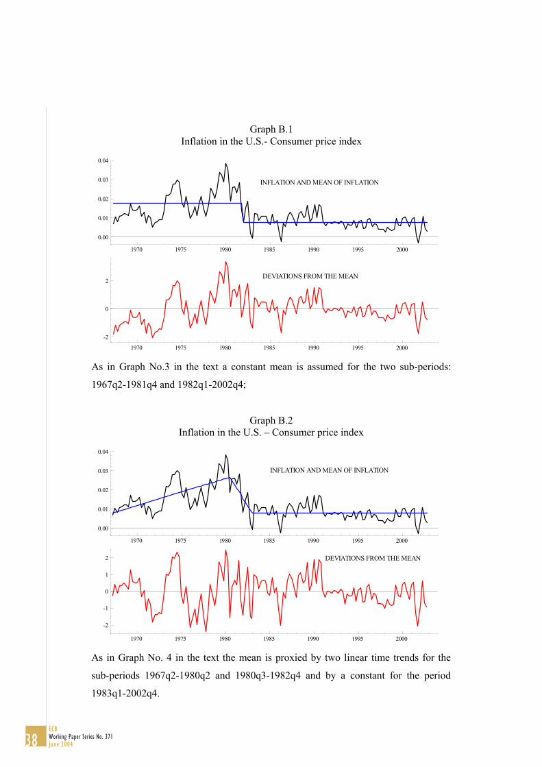
Graph B.1 Inflation in the U.S.- Consumer price index
1970 1975 1980 1985 1990 1995 2000
0.00
0.01
0.02
0.03
0.04
INFLATION AND MEAN OF INFLATION
1970 1975 1980 1985 1990 1995 2000
-2
0
2DEVIATIONS FROM THE MEAN
As in Graph No.3 in the text a constant mean is assumed for the two sub-periods:
1967q2-1981q4 and 1982q1-2002q4;
Graph B.2 Inflation in the U.S. – Consumer price index
1970 1975 1980 1985 1990 1995 2000
0.00
0.01
0.02
0.03
0.04
INFLATION AND MEAN OF INFLATION
1970 1975 1980 1985 1990 1995 2000
-2
-1
0
1
2 DEVIATIONS FROM THE MEAN
As in Graph No. 4 in the text the mean is proxied by two linear time trends for the
sub-periods 1967q2-1980q2 and 1980q3-1982q4 and by a constant for the period
1983q1-2002q4.
38
ECBWorking Paper Series No. 371June 2004

Graph B.3 Inflation in the U.S. – Consumer price index
1970 1975 1980 1985 1990 1995 2000
0.00
0.01
0.02
0.03
0.04
INFLATION AND MEAN OF INFLATION
1970 1975 1980 1985 1990 1995 2000
-2
-1
0
1
2
3
DEVIATIONS FROM THE MEAN
As in Graph No. 2 in the text the mean is proxied by two linear time trends for the two
sub-periods 1967q2-1980q2 and 1980q3-1982q4 an by a constant for the period
1983q1-2002q4 with a break in 1991q2.
Graph B.4 Inflation in the U.S. – Consumer price index
1970 1975 1980 1985 1990 1995 2000
0.00
0.01
0.02
0.03
0.04
INFLATION AND MEAN OF INFLATION
1970 1975 1980 1985 1990 1995 2000
-0.01
0.00
0.01 DEVIATIONS FROM THE MEAN
As in Graph No. 5 in the text the mean is proxied by the HP filtered series (with
). λ = 1600
39
ECBWorking Paper Series No. 371
June 2004

Graph B.5 Inflation in the U.S. – Consumer price index
1970 1975 1980 1985 1990 1995 2000
0.00
0.01
0.02
0.03
0.04
INFLATION AND MEAN OF INFLATION
1970 1975 1980 1985 1990 1995 2000
-0.010
-0.005
0.000
0.005
0.010 DEVIATIONS FROM THE MEAN
As in Graph No. 6 in the text the mean is proxied by the 13 terms centred moving
average.
Graph B.6
Inflation in the E.A. – Consumer price index
1970 1975 1980 1985 1990 1995 2000
0.01
0.02
0.03 INFLATION AND MEAN OF INFLATION
1970 1975 1980 1985 1990 1995 2000
-2
0
2 DEVIATIONS FROM THE MEAN
As in Graph No. 3 in the text a constant mean is assumed for the two sub-periods:
1967q2-1983q4 and 1984q1-2002q4;
40
ECBWorking Paper Series No. 371June 2004
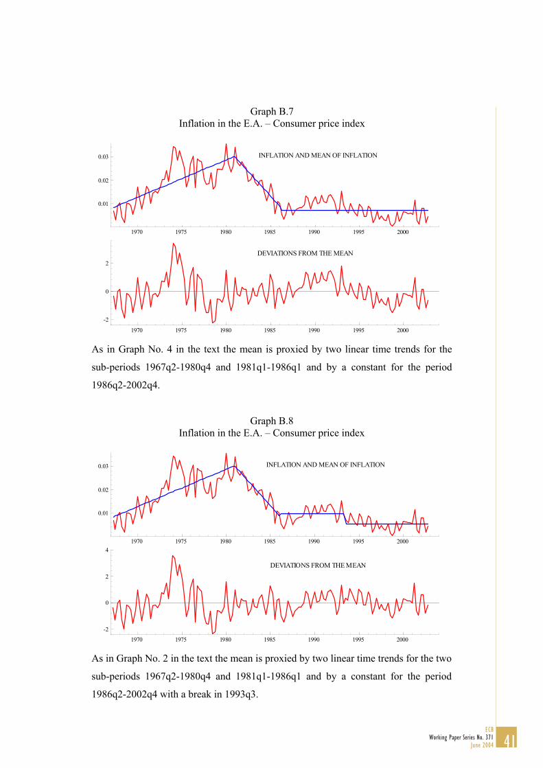
Graph B.7 Inflation in the E.A. – Consumer price index
1970 1975 1980 1985 1990 1995 2000
0.01
0.02
0.03 INFLATION AND MEAN OF INFLATION
1970 1975 1980 1985 1990 1995 2000
-2
0
2DEVIATIONS FROM THE MEAN
As in Graph No. 4 in the text the mean is proxied by two linear time trends for the
sub-periods 1967q2-1980q4 and 1981q1-1986q1 and by a constant for the period
1986q2-2002q4.
Graph B.8 Inflation in the E.A. – Consumer price index
1970 1975 1980 1985 1990 1995 2000
0.01
0.02
0.03 INFLATION AND MEAN OF INFLATION
1970 1975 1980 1985 1990 1995 2000
-2
0
2
4
DEVIATIONS FROM THE MEAN
As in Graph No. 2 in the text the mean is proxied by two linear time trends for the two
sub-periods 1967q2-1980q4 and 1981q1-1986q1 and by a constant for the period
1986q2-2002q4 with a break in 1993q3.
41
ECBWorking Paper Series No. 371
June 2004
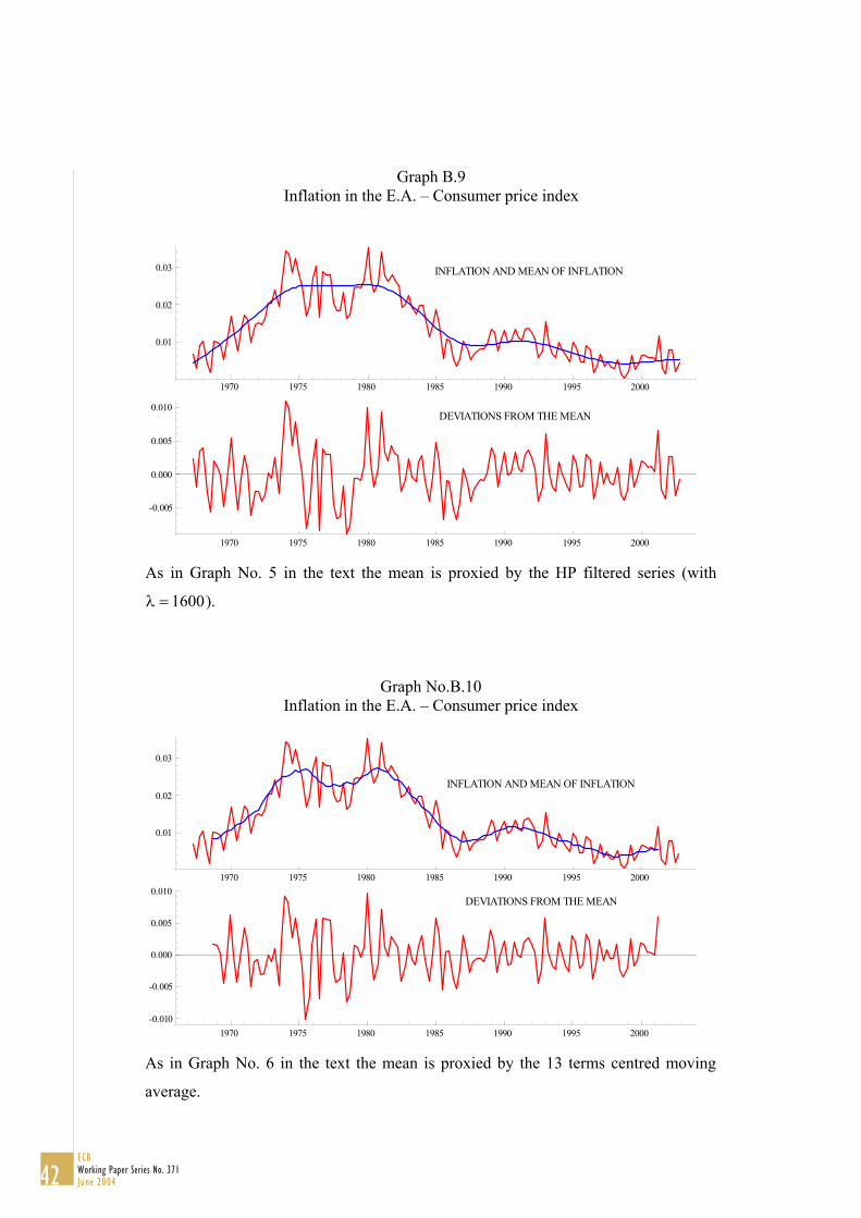
Graph B.9 Inflation in the E.A. – Consumer price index
1970 1975 1980 1985 1990 1995 2000
0.01
0.02
0.03 INFLATION AND MEAN OF INFLATION
1970 1975 1980 1985 1990 1995 2000
-0.005
0.000
0.005
0.010DEVIATIONS FROM THE MEAN
As in Graph No. 5 in the text the mean is proxied by the HP filtered series (with
). λ = 1600
Graph No.B.10 Inflation in the E.A. – Consumer price index
1970 1975 1980 1985 1990 1995 2000
0.01
0.02
0.03
INFLATION AND MEAN OF INFLATION
1970 1975 1980 1985 1990 1995 2000-0.010
-0.005
0.000
0.005
0.010DEVIATIONS FROM THE MEAN
As in Graph No. 6 in the text the mean is proxied by the 13 terms centred moving
average.
42
ECBWorking Paper Series No. 371June 2004
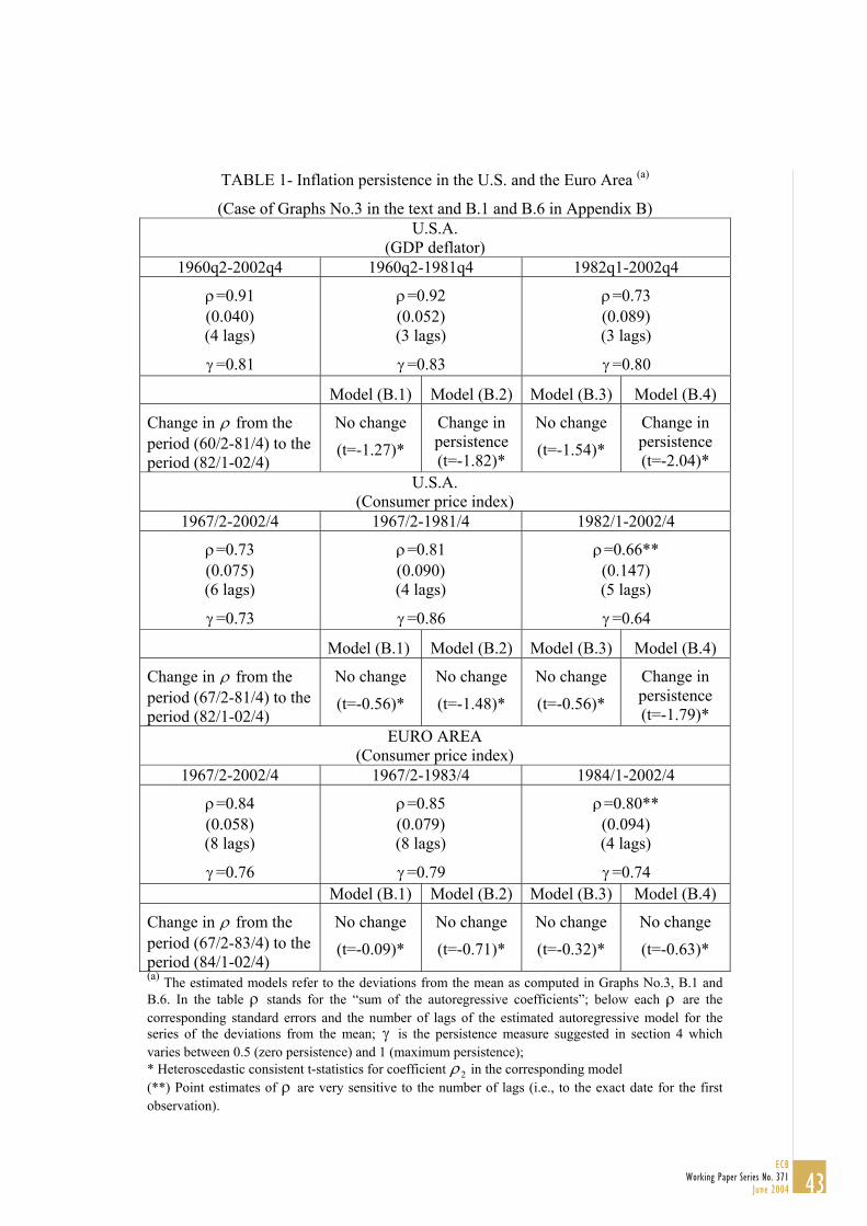
TABLE 1- Inflation persistence in the U.S. and the Euro Area (a)
(Case of Graphs No.3 in the text and B.1 and B.6 in Appendix B) U.S.A.
(GDP deflator) 1960q2-2002q4 1960q2-1981q4 1982q1-2002q4
ρ=0.91 (0.040) (4 lags)
γ =0.81
ρ=0.92 (0.052) (3 lags)
γ =0.83
ρ=0.73 (0.089) (3 lags)
γ =0.80 Model (B.1) Model (B.2) Model (B.3) Model (B.4)
Change in ρ from the period (60/2-81/4) to the period (82/1-02/4)
No change
(t=-1.27)*
Change in persistence (t=-1.82)*
No change
(t=-1.54)*
Change in persistence (t=-2.04)*
U.S.A. (Consumer price index)
1967/2-2002/4 1967/2-1981/4 1982/1-2002/4
ρ=0.73 (0.075) (6 lags)
γ =0.73
ρ=0.81 (0.090) (4 lags)
γ =0.86
ρ=0.66** (0.147) (5 lags)
γ =0.64 Model (B.1) Model (B.2) Model (B.3) Model (B.4)
Change in ρ from the period (67/2-81/4) to the period (82/1-02/4)
No change
(t=-0.56)*
No change
(t=-1.48)*
No change
(t=-0.56)*
Change in persistence (t=-1.79)*
EURO AREA (Consumer price index)
1967/2-2002/4 1967/2-1983/4 1984/1-2002/4
ρ=0.84 (0.058) (8 lags)
γ =0.76
ρ=0.85 (0.079) (8 lags)
γ =0.79
ρ=0.80** (0.094) (4 lags)
γ =0.74 Model (B.1) Model (B.2) Model (B.3) Model (B.4)
Change in ρ from the period (67/2-83/4) to the period (84/1-02/4)
No change
(t=-0.09)*
No change
(t=-0.71)*
No change
(t=-0.32)*
No change
(t=-0.63)* (a) The estimated models refer to the deviations from the mean as computed in Graphs No.3, B.1 and B.6. In the table ρ stands for the “sum of the autoregressive coefficients”; below each ρ are the corresponding standard errors and the number of lags of the estimated autoregressive model for the series of the deviations from the mean; γ is the persistence measure suggested in section 4 which varies between 0.5 (zero persistence) and 1 (maximum persistence); * Heteroscedastic consistent t-statistics for coefficient ρ2 in the corresponding model (**) Point estimates of ρ are very sensitive to the number of lags (i.e., to the exact date for the first observation).
43
ECBWorking Paper Series No. 371
June 2004

TABLE 2 – Persistence in the U.S. and the Euro Area (a) (Case of Graphs No.4 in the text and B.2 and B.7 in Appendix B)
U.S.A. (GDP deflator)
1960/2-2002/4 1960/2-1980/4 1981/1-2002/4 1960/2-1983/1 1983/2-2002/4
ρ=0.58 (0.090) (6 lags)
γ =0.70
ρ=0.45 (0.139) (6 lags)
γ =0.66
ρ=0.79 (0.099) (3 lags)
γ =0.74
ρ=0.45 (0.135) (6 lags)
γ =0.64
ρ=0.80 (0.104) (4 lags)
γ =0.77 Model (B.1) Model (B.2) Model (B.3) Model (B.4)
Change in ρ from the period (60/2-80/4) to the period (81/1-02/4).
No change
(t=1.53)*
No change
(t=0.20)*
No change
(t=1.54)*
No change
(t=0.43)*
Change in ρ from the period (60/2-83/1) for the period (83/2-02/4).
No change
(t=1.57)*
No change
(t=0.61)*
No change
(t=1.47)*
No change
(t=0.60)*
U.S.A. (Consumer price index)
1967/2-2002/4 1967/2-1980/2 1980/3-2002/4 1967/2-1982/4 1983/1-2002/4
ρ=0.54 (0.010) (6 lags)
γ =0.66
ρ=0.63** (0.117) (5 lags)
γ =0.75
ρ=0.53 (0.137) (3 lags)
γ =0.61
ρ=0.67** (0.128) (4 lags)
γ =0.71
ρ=0.63 (0.129) (3 lags)
γ =0.63 Model (B.1) Model (B.2) Model (B.3) Model (B.4)
Change in ρ from the period (67/2-80/2) to the period (80/3-02/4)(b).
No change
(t=-0.28)*
Change in persistence (t=-2.46)*
No change
(t=-0.10)*
Change in persistence (t=-1.79)*
EURO AREA (Consumer price index)
1967/2-2002/4 1967/2-1980/4 1981/1-2002/4 1967/2-1986/1 1986/2-2002/4
ρ=0.80 (0.089) (8 lags)
γ =0.71
ρ=0.81 (0.155) (8 lags)
γ =0.75
ρ=0.85 (0.102) (4 lags)
γ =0.68
ρ=0.76 (0.136) (8 lags)
γ =0.67
ρ=0.88 (0.105) (4 lags)
γ =0.75 Model (B.1) Model (B.2) Model (B.3) Model (B.4)
Change in ρ from the period (67/2-80/4) to the period (81/1-02/4)(c).
No change
(t=0.19)*
No change
(t=-0.78)*
No change
(t=0.28)*
No change
(t=-0.50)* (a) See table 1 for explanations.(b) There is no change in persistence when we compare the periods (1967/2-1982/4) and (1983/1-2002/4); (c) There is also no change in persistence when we compare the periods (1967/2-1986/1) and (1986/2-2002/4);
44
ECBWorking Paper Series No. 371June 2004
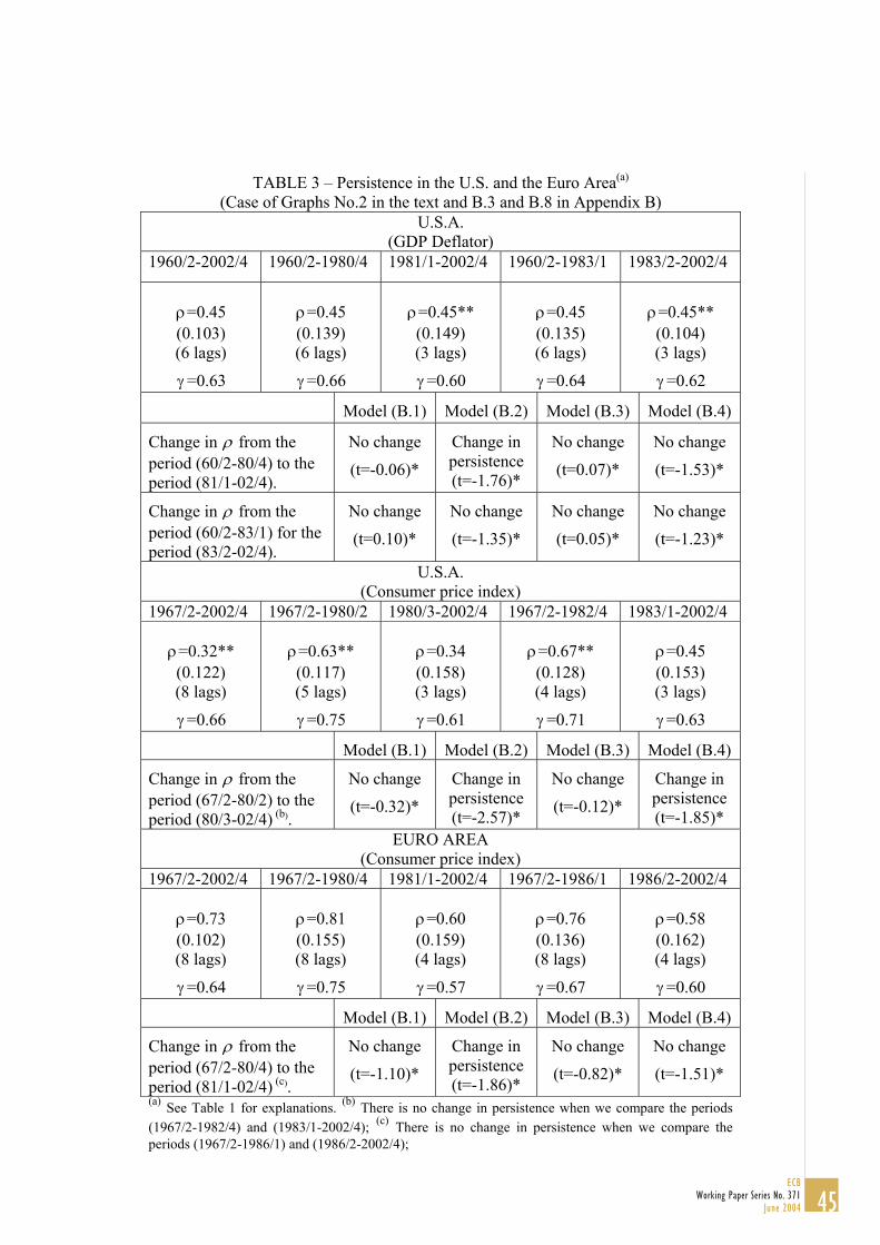
TABLE 3 – Persistence in the U.S. and the Euro Area(a) (Case of Graphs No.2 in the text and B.3 and B.8 in Appendix B)
U.S.A. (GDP Deflator)
1960/2-2002/4 1960/2-1980/4 1981/1-2002/4 1960/2-1983/1 1983/2-2002/4
ρ=0.45 (0.103) (6 lags)
γ =0.63
ρ=0.45 (0.139) (6 lags)
γ =0.66
ρ=0.45** (0.149) (3 lags)
γ =0.60
ρ=0.45 (0.135) (6 lags)
γ =0.64
ρ=0.45** (0.104) (3 lags)
γ =0.62
Model (B.1) Model (B.2) Model (B.3) Model (B.4)
Change in ρ from the period (60/2-80/4) to the period (81/1-02/4).
No change
(t=-0.06)*
Change in persistence (t=-1.76)*
No change
(t=0.07)*
No change
(t=-1.53)*
Change in ρ from the period (60/2-83/1) for the period (83/2-02/4).
No change
(t=0.10)*
No change
(t=-1.35)*
No change
(t=0.05)*
No change
(t=-1.23)*
U.S.A. (Consumer price index)
1967/2-2002/4 1967/2-1980/2 1980/3-2002/4 1967/2-1982/4 1983/1-2002/4
ρ=0.32** (0.122) (8 lags)
γ =0.66
ρ=0.63** (0.117) (5 lags)
γ =0.75
ρ=0.34 (0.158) (3 lags)
γ =0.61
ρ=0.67** (0.128) (4 lags)
γ =0.71
ρ=0.45 (0.153) (3 lags)
γ =0.63
Model (B.1) Model (B.2) Model (B.3) Model (B.4)
Change in ρ from the period (67/2-80/2) to the period (80/3-02/4) (b).
No change
(t=-0.32)*
Change in persistence (t=-2.57)*
No change
(t=-0.12)*
Change in persistence (t=-1.85)*
EURO AREA (Consumer price index)
1967/2-2002/4 1967/2-1980/4 1981/1-2002/4 1967/2-1986/1 1986/2-2002/4
ρ=0.73 (0.102) (8 lags)
γ =0.64
ρ=0.81 (0.155) (8 lags)
γ =0.75
ρ=0.60 (0.159) (4 lags)
γ =0.57
ρ=0.76 (0.136) (8 lags)
γ =0.67
ρ=0.58 (0.162) (4 lags)
γ =0.60
Model (B.1) Model (B.2) Model (B.3) Model (B.4)
Change in ρ from the period (67/2-80/4) to the period (81/1-02/4) (c).
No change
(t=-1.10)*
Change in persistence (t=-1.86)*
No change
(t=-0.82)*
No change
(t=-1.51)* (a) See Table 1 for explanations. (b) There is no change in persistence when we compare the periods (1967/2-1982/4) and (1983/1-2002/4); (c) There is no change in persistence when we compare the periods (1967/2-1986/1) and (1986/2-2002/4);
45
ECBWorking Paper Series No. 371
June 2004
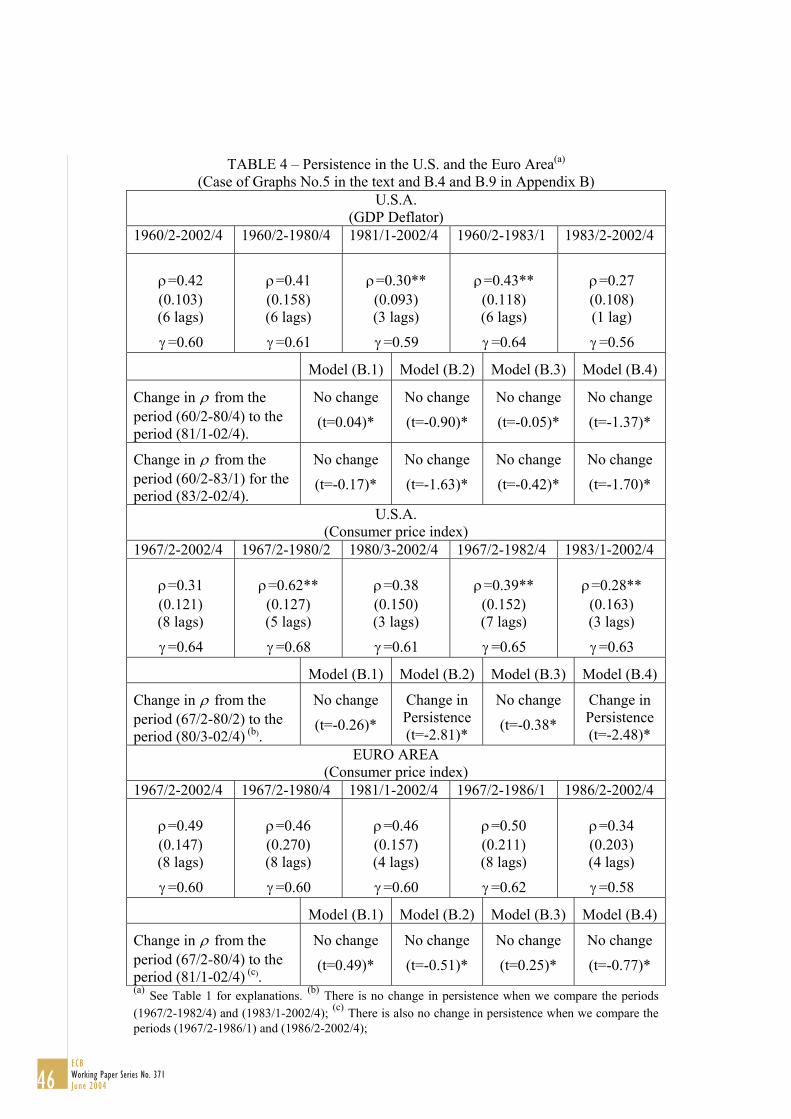
TABLE 4 – Persistence in the U.S. and the Euro Area(a) (Case of Graphs No.5 in the text and B.4 and B.9 in Appendix B)
U.S.A. (GDP Deflator)
1960/2-2002/4 1960/2-1980/4 1981/1-2002/4 1960/2-1983/1 1983/2-2002/4
ρ=0.42 (0.103) (6 lags)
γ =0.60
ρ=0.41 (0.158) (6 lags)
γ =0.61
ρ=0.30** (0.093) (3 lags)
γ =0.59
ρ=0.43** (0.118) (6 lags)
γ =0.64
ρ=0.27 (0.108) (1 lag)
γ =0.56
Model (B.1) Model (B.2) Model (B.3) Model (B.4)
Change in ρ from the period (60/2-80/4) to the period (81/1-02/4).
No change
(t=0.04)*
No change
(t=-0.90)*
No change
(t=-0.05)*
No change
(t=-1.37)*
Change in ρ from the period (60/2-83/1) for the period (83/2-02/4).
No change
(t=-0.17)*
No change
(t=-1.63)*
No change
(t=-0.42)*
No change
(t=-1.70)*
U.S.A. (Consumer price index)
1967/2-2002/4 1967/2-1980/2 1980/3-2002/4 1967/2-1982/4 1983/1-2002/4
ρ=0.31 (0.121) (8 lags)
γ =0.64
ρ=0.62** (0.127) (5 lags)
γ =0.68
ρ=0.38 (0.150) (3 lags)
γ =0.61
ρ=0.39** (0.152) (7 lags)
γ =0.65
ρ=0.28** (0.163) (3 lags)
γ =0.63
Model (B.1) Model (B.2) Model (B.3) Model (B.4)
Change in ρ from the period (67/2-80/2) to the period (80/3-02/4) (b).
No change
(t=-0.26)*
Change in Persistence (t=-2.81)*
No change
(t=-0.38*
Change in Persistence (t=-2.48)*
EURO AREA (Consumer price index)
1967/2-2002/4 1967/2-1980/4 1981/1-2002/4 1967/2-1986/1 1986/2-2002/4
ρ=0.49 (0.147) (8 lags)
γ =0.60
ρ=0.46 (0.270) (8 lags)
γ =0.60
ρ=0.46 (0.157) (4 lags)
γ =0.60
ρ=0.50 (0.211) (8 lags)
γ =0.62
ρ=0.34 (0.203) (4 lags)
γ =0.58
Model (B.1) Model (B.2) Model (B.3) Model (B.4)
Change in ρ from the period (67/2-80/4) to the period (81/1-02/4) (c).
No change
(t=0.49)*
No change
(t=-0.51)*
No change
(t=0.25)*
No change
(t=-0.77)* (a) See Table 1 for explanations. (b) There is no change in persistence when we compare the periods (1967/2-1982/4) and (1983/1-2002/4); (c) There is also no change in persistence when we compare the periods (1967/2-1986/1) and (1986/2-2002/4);
46
ECBWorking Paper Series No. 371June 2004
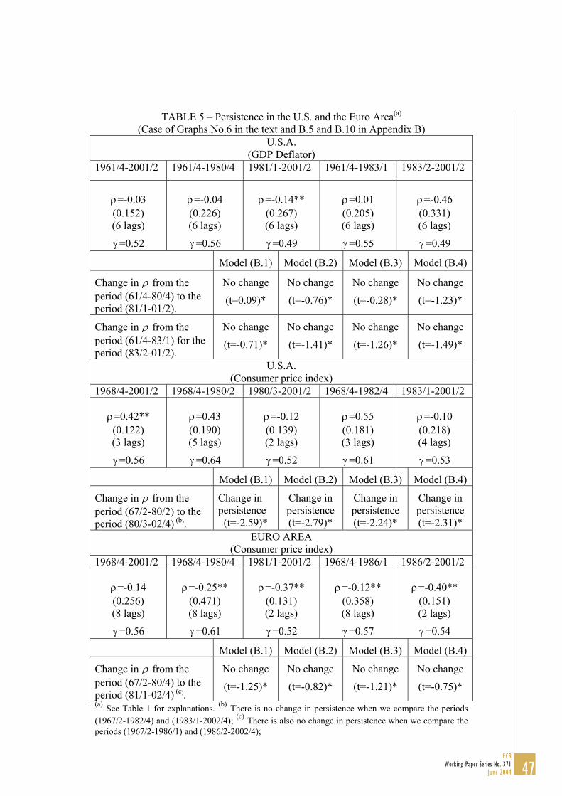
TABLE 5 – Persistence in the U.S. and the Euro Area(a) (Case of Graphs No.6 in the text and B.5 and B.10 in Appendix B)
U.S.A. (GDP Deflator)
1961/4-2001/2 1961/4-1980/4 1981/1-2001/2 1961/4-1983/1 1983/2-2001/2
ρ=-0.03 (0.152) (6 lags)
γ =0.52
ρ=-0.04 (0.226) (6 lags)
γ =0.56
ρ=-0.14**
(0.267) (6 lags)
γ =0.49
ρ=0.01 (0.205) (6 lags)
γ =0.55
ρ=-0.46 (0.331) (6 lags)
γ =0.49
Model (B.1) Model (B.2) Model (B.3) Model (B.4)
Change in ρ from the period (61/4-80/4) to the period (81/1-01/2).
No change
(t=0.09)*
No change
(t=-0.76)*
No change
(t=-0.28)*
No change
(t=-1.23)*
Change in ρ from the period (61/4-83/1) for the period (83/2-01/2).
No change
(t=-0.71)*
No change
(t=-1.41)*
No change
(t=-1.26)*
No change
(t=-1.49)*
U.S.A. (Consumer price index)
1968/4-2001/2 1968/4-1980/2 1980/3-2001/2 1968/4-1982/4 1983/1-2001/2
ρ=0.42** (0.122) (3 lags)
γ =0.56
ρ=0.43 (0.190) (5 lags)
γ =0.64
ρ=-0.12 (0.139) (2 lags)
γ =0.52
ρ=0.55 (0.181) (3 lags)
γ =0.61
ρ=-0.10 (0.218) (4 lags)
γ =0.53
Model (B.1) Model (B.2) Model (B.3) Model (B.4)
Change in ρ from the period (67/2-80/2) to the period (80/3-02/4) (b).
Change in persistence
(t=-2.59)*
Change in persistence (t=-2.79)*
Change in persistence (t=-2.24)*
Change in persistence (t=-2.31)*
EURO AREA (Consumer price index)
1968/4-2001/2 1968/4-1980/4 1981/1-2001/2 1968/4-1986/1 1986/2-2001/2
ρ=-0.14 (0.256) (8 lags)
γ =0.56
ρ=-0.25**
(0.471) (8 lags)
γ =0.61
ρ=-0.37**
(0.131) (2 lags)
γ =0.52
ρ=-0.12**
(0.358) (8 lags)
γ =0.57
ρ=-0.40**
(0.151) (2 lags)
γ =0.54
Model (B.1) Model (B.2) Model (B.3) Model (B.4)
Change in ρ from the period (67/2-80/4) to the period (81/1-02/4) (c).
No change
(t=-1.25)*
No change
(t=-0.82)*
No change
(t=-1.21)*
No change
(t=-0.75)* (a) See Table 1 for explanations. (b) There is no change in persistence when we compare the periods (1967/2-1982/4) and (1983/1-2002/4); (c) There is also no change in persistence when we compare the periods (1967/2-1986/1) and (1986/2-2002/4);
47
ECBWorking Paper Series No. 371
June 2004
European Central Bank working paper series
For a complete list of Working Papers published by the ECB, please visit the ECB�s website(http://www.ecb.int).
314 “Exchange rate risks and asset prices in a small open economy” by A. Derviz, March 2004.
315 “Option-implied asymmetries in bond market expectations around monetary policy actions of the ECB” by S. Vähämaa, March 2004.
321 “Frequency domain principal components estimation of fractionally cointegrated processes”
by C. Morana, March 2004.
322 “Modelling inflation in the euro area” by E. S. Jansen, March 2004.
323 “On the indeterminacy of New-Keynesian economics” by A. Beyer and R. E. A. Farmer, March 2004.
324 “Fundamentals and joint currency crises” by P. Hartmann, S. Straetmans and C. G. de Vries, March 2004.
325 “What are the spill-overs from fiscal shocks in Europe? An empirical analysis” by M. Giuliodori
and R. Beetsma, March 2004.
326 “The great depression and the Friedman-Schwartz hypothesis” by L. Christiano, R. Motto and
M. Rostagno, March 2004.
327 “Diversification in euro area stock markets: country versus industry” by G. A. Moerman, April 2004.
328 “Non-fundamental exchange rate volatility and welfare” by R. Straub and I. Tchakarov, April 2004.
329 “On the determinants of euro area FDI to the United States: the knowledge-capital-Tobin's Q framework,
by R. A. De Santis, R. Anderton and A. Hijzen, April 2004.
330 “The demand for euro area currencies: past, present and future” by B. Fischer, P. Köhler and F. Seitz, April 2004.
331 “How frequently do prices change? evidence based on the micro data underlying the Belgian CPI” by
L. Aucremanne and E. Dhyne, April 2004.
332 “Stylised features of price setting behaviour in Portugal: 1992-2001” by M. Dias, D. Dias
and P. D. Neves, April 2004.
316 “Cooperation in international banking supervision” by C. Holthausen and T. Rønde, March 2004.
317 “Fiscal policy and inflation volatility” by P. C. Rother, March 2004.
318 “Gross job flows and institutions in Europe” by R. Gómez-Salvador, J. Messina and G. Vallanti, March 2004.
319 “Risk sharing through financial markets with endogenous enforcement of trades” by T. V. Köppl, March 2004.
320 “Institutions and service employment: a panel study for OECD countries” by J. Messina, March 2004.
333 “The pricing behaviour of Italian firms: New survey evidence on price stickiness” by
S. Fabiani, A. Gattulli and R. Sabbatini, April 2004.
48ECBWorking Paper Series No. 371June 2004
334 “Is inflation persistence intrinsic in industrial economies?” by A. T. Levin and J. M. Piger, April 2004.
335 “Has eura-area inflation persistence changed over time?” by G. O’Reilly and K. Whelan, April 2004.
336 “The great inflation of the 1970s” by F. Collard and H. Dellas, April 2004.
337 “The decline of activist stabilization policy: Natural rate misperceptions, learning and expectations” by
A. Orphanides and J. C. Williams, April 2004.
338 “The optimal degree of discretion in monetary policy” by S. Athey, A. Atkeson and P. J. Kehoe, April 2004.
339 “Understanding the effects of government spending on consumption” by J. Galí, J. D. López-Salido
and J. Vallés, April 2004.
340 “Indeterminacy with inflation-forecast-based rules in a two-bloc model” by N. Batini, P.Levine
and J. Pearlman, April 2004.
341 “Benefits and spillovers of greater competition in Europe: A macroeconomic assessment” by T. Bayoumi,
D. Laxton and P. Pesenti, April 2004.
342 “Equal size, equal role? Interest rate interdependence between the euro area and the United States” by
M. Ehrmann and M. Fratzscher, April 2004.
343 “Monetary discretion, pricing complementarity and dynamic multiple equilibria” by R. G. King
and A. L. Wolman, April 2004.
344 “Ramsey monetary policy and international relative prices” by E. Faia and T. Monacelli, April 2004.
345 “Optimal monetary and fiscal policy: A linear-quadratic approach” by P. Benigno and M. Woodford, April 2004.
346 “Perpetual youth and endogenous labour supply: a problem and a possible solution” by G. Ascari and
N. Rankin, April 2004.
347 “Firms’ investment decisions in response to demand and price uncertainty” by C. Fuss
and P. Vermeulen, April 2004.
348 “Financial openness and growth: Short-run gain, long-run pain?” by M. Fratzscher and M. Bussiere, April 2004.
349 “Estimating the rank of the spectral density matrix” by G. Camba-Mendez and G. Kapetanios, April 2004.
350 “Exchange-rate policy and the zero bound on nominal interest rates” by G. Camba-Mendez
and G. Kapetanios, April 2004.
351 “Interest rate determination in the interbank market” by V. Gaspar, G. P. Quirós and
H. R. Mendizábal, April 2004.
352 “Forecasting inflation with thick models and neural networks” by P. McNelis and
P. McAdam, April 2004.
49ECB
Working Paper Series No. 371June 2004
353 “Towards the estimation of equilibrium exchange rates for CEE acceding countries: methodological
issues and a panel cointegration perspective” by F. Maeso-Fernandez, C. Osbat and B. Schnatz, April 2004.
354 “Taking stock: monetary policy transmission to equity markets” by M. Ehrmann and M. Fratzscher, May 2004.
355 “Production interdependence and welfare” by K. X. D. Huang and Z. Liu, May 2004.
356 “Developing a euro area accounting matrix: issues and applications” by T. Jellema, S. Keuning,P. McAdam and R. Mink, May 2004.
357 “Seasonal adjustment and the detection of business cycle phases” by A. M. Mir andD. R. Osborn, May 2004.
358 “Did the pattern of aggregate employment growth change in the euro area in thelate 1990s?” by G. Mourre, May 2004.
359 “The longer term refinancing operations of the ECB” by T. Linzert, D. Nautz and U. Bindseil,May 2004.
360 “Optimal monetary policy rules for the euro area: an analysis using the area wide model”by A. Dieppe, K. Küster and P. McAdam, May 2004.
361 “Excess reserves and the implementation of monetary policy of the ECB” by U. Bindseil,G. Camba-Mendez, A. Hirsch and B. Weller, May 2004.
362 “Oil price shocks and real GDP growth: empirical evidence for some OECD countries” byR. Jiménez-Rodríguez and M. Sánchez, May 2004.
363 “Communication and exchange rate policy” by M. Fratzscher, May 2004.
364 “Asset price booms and monetary policy” by C. Detken and F. Smets, May 2004.
365 “Exchange rates and fundamentals: new evidence from real-time data” by M. Ehrmann andM. Fratzscher, May 2004.
366 “The informational content of over-the-counter currency options” by P. Christoffersen andS. Mazzotta, June 2004.
367 “Factor substitution and factor augmenting technical: progress in the US: a normalized supply-side system approach” by R Klump, P. McAdam and A. Willman, June 2004.
368 “Capital quality improvement and the sources of growth in the euro area” by P. Sakellaris and F. W. Vijselaar, June 2004.
369 “Sovereign risk premia in the European government bond market” by K. Bernoth, J. von Hagen and L. Schuknecht, June 2004.
370 “Inflation persistence during periods of structural change: an assessment using Greek data” by G. Hondroyiannis and S. Lazaretou, June 2004.
371 “Inflation persistence: facts or artefacts?” by C. R. Marques, June 2004.
50ECBWorking Paper Series No. 371June 2004
