working paper series issn 1753 - 5816 please cite this

Please cite this paper as:

No. 177

Welfare Analysis of Changing Food Prices: A Nonparametric

Examination of Export Ban on Rice in India

by

Ben Groom and Mehroosh Tak

(January, 2013)

Department of Economics School of Oriental and African Studies

London WC1H 0XG

Phone: + 44 (0)20 7898 4730 Fax: 020 7898 4759

E-mail: [email protected] http://www.soas.ac.uk/economics/

D

epar

tmen

t of

Eco

nom

ics ISSN 1753 - 5816

Groom, B. and Tak, M. (2013), “Welfare Analysis of Changing Food Prices: A Nonparametric Examination of Export Ban on Rice in India” SOAS Department of Economics Working Paper Series, No. 177, The School of Oriental and African Studies.

Working Paper Series

The SOAS Department of Economics Working Paper Series is published electronically by The School of Oriental and African Studies-University of London. ©Copyright is held by the author or authors of each working paper. SOAS DoEc Working Papers cannot be republished, reprinted or reproduced in any format without the permission of the paper’s author or authors. This and other papers can be downloaded without charge from: SOAS Department of Economics Working Paper Series at http://www.soas.ac.uk/economics/research/workingpapers/ Design and layout: O. González Dávila

SOAS Department of Economics Working Paper Series No 177 - 2013

1

Welfare Analysis of Changing Food Prices: A Nonparametric Examination of Export Ban on Rice in India

Ben Groom and Mehroosh Tak

Abstract

During the world food crisis of 2007-08, the price of staples soared rapidly. Higher food price

impacts poor households more as they spend approximately three quarters of their income on

food. Together rice and wheat provide more than 50% of the calorific intake in India. Apart

from providing food security, millions of poor and small farmers depend on rice for their

livelihoods. Using Indian Consumer Household Expenditure surveys for the years 2007-08

and 2009-10 the paper analyses the welfare generated by a ban on export of rice by the Indian

government. The paper finds that the net impact of the ban on export of rice was positive, as

it was able to cushion the Indian population (87% of whom are net consumers) from the

adverse effects of the crisis. It also found that the poor in India aren’t homogeneous in nature.

The majority of the rice-producing households that stand to gain from increased prices are

relatively poor farmers. At the same time, the poor households that do not cultivate rice are

most affected by price increase, as their budget share of rice is higher than richer households,

who are more resilient to price rise. In particular, the wage labourers are affected

significantly.

JEL classification: Q11, Q12, Q17, Q18

Keywords: Food price shock, India, rice, nonparametric estimation, poverty, welfare analysis

1. Introduction

Since the world food crisis of 2007-08, increasing food prices have agitated civilians across

the world, leading to dethroning of political powers in some countries. In India, the

government has always cushioned the agriculture sector due to the sector’s contribution to the

GDP, and also because of its political importance to every Indian government that has been in

power. Agricultural pricing policies not only impact different aspects of the economy

differently, but also vary in scale amongst different sections of the poor. Datt and


2

Ravallion’s1 study on India for the period 1958–94 reports that in the long-run the price effect

of food crop productivity (followed by the wage effect) is better at reducing poverty relative

to the direct impact of increase in farm incomes, which dominates this relationship in the

short-run. The duality of change in price of food grains leads to conflicting policy objectives.

A decline in price can adversely affect farmers, but at the same time increase the

ability of the poor to consume more, leading to an improved standard of living. Neo-populist

economists such as Lipton2 and Griffin suggest that lower prices of staples benefit the rural

poor, as they are net consumers of food. While a rise in price tends to create an "urban bias",

where rich households are better able to provide for them. In such a scenario, the neo-

populists call for greater government intervention in support of the farmers. However,

neoclassical economists assert that higher pricing policies intended to boost production are

important as the rural poor "still rely on selling their produce for a significant part of their

income So, changes in market prices matter”3 to reduce rural poverty. Both the schools of

thought tend to ignore the diversity amongst the poor. Thus, policy makers need a better

understanding of the section of poor they are targeting than simply relying on the trickle-

down effects of pricing policy. In India, the agriculture sector employs more than 58% of the

total workforce and contributed 15% towards the GDP in 2009-104. Due to the extent of

dependency of the Indian economy and population on the agriculture sector it is important to

determine which groups are most vulnerable, and how they are affected by agriculture price

policies.

The purpose of this paper is to measure the impact of changing food prices, through a

nonparametric examination of the Indian government’s move to ban the export of rice in the

light of the world food crisis of 2007-08. The paper follows Angus Deaton’s5 non-parametric

techniques for regression and density estimation on Indian Consumer Household Expenditure

surveys for the years 2007-08 and 2009-10. Section 2 gives an overview of agriculture sector

in India and volatility of rice prices between 2007 and 2010. Section 3 describes the empirical

framework for the analysis. This section also explains the source of the dataset and the

censored data problem faced. The results are analysed in section 4. Section 5 is the

conclusion. The paper concludes that the export ban had a net positive impact on the Indian

1 Cited in WDR (2008) p.33 2 Lipton (1986) 3 World Bank (1994) p.167 4 Indian Economic Survey (2011-12) 5 Deaton (1989)


3

population, 87% of whom are net consumers of rice. We also find that the poor in India are

heterogeneous in nature. Thus agriculture-pricing policies do not have a homogenous impact

on the poor. Majority of rice producers are poor farmers who benefited from the rise in price

of rice, while the wage labourers were worse off.

2. Overview of the Indian Agriculture Sector

For an agrarian economy such as India, where three-fifths of the labour force depends on the

agriculture sector for livelihood, the agriculture sector is not only important for economic

growth, but also to maintain political and social stability in the country. Thus, historically the

various Indian governments have treated this sector with a lot of love in the form of subsidies

and tax relaxations6.

In 2007-08 the price of rice almost doubled across the globe. Foreseeing a global rise in rice

prices, the Indian government reacted by exercising an import ban on non-basmati rice in

February 2008 and increased export tariffs on basmati rice in April 20087. Where globally

prices more than doubled, in India they only increased by 40% from 2007-2010. Compared to

the rest of the world the impact of the world food crisis of 2007-08 on the Indian economy

was low, due to the self-sufficiency and cushioning policies of the Indian government since

independence. India’s protectionist agricultural policies have been criticised by advocates of

free trade. According to the Food and Agriculture Organization (FAO), India’s decision to

ban the export of rice even with surplus quantities of it was a political move rather than a

result of real shortage of grain8. Traditional trade models suggest that free trade maximises

economic welfare. However, when the aim is to maximise national welfare, free trade may

not be the obvious policy choice for a developing nation. The objective of the export ban was

to increase supply of rice within the country and hence contain the increasing price of rice to

insulate the consumers against the negative impact of rising food prices. At the same time the

Indian rice producers would receive lower prices relative to the rest of the world, creating a

possible negative welfare impact for farmers. The ban was uplifted in February 20129.

6 James (1992) p.224 7 FAO (2009) 8 FAO (2009) p.36 9 The Economic Times, February 2012


4

0%

20%

40%

60%

80%

100%

120%

140%

160%

Sep‐07 Dec‐07 Mar‐08 Jun‐08 Sep‐08 Dec‐08 Mar‐09 Jun‐09 Sep‐09 Dec‐09 Mar‐10 Jun‐10

Percentage

Chan

ge in

Prices

Prices change relative to July 2007.Source: Ministry of Commerce and Industry for India and FAO International Commodity Prices Data Base for World Prices

Fig.1. Change in Rice Prices

World

India

Export Ban on Rice Implemented

Figure 1 shows the change in price of rice relative to July 2007 for India and worldwide. The

horizontal red line indicates the implementation of ban on exports on rice in India in February

2008. In India, the price of rice increased by 11% between July 2007 and March 2008.

During the same period, world rice prices10 doubled. In June 2008 prices in India increased

by 13% from July 2007 whereas, globally, prices increased by 150%.

3. Methodology and Data

The paper is based on nonparametric approach11 for regression and density estimation and

heavily relies on graphical representation of the relationships between indicators of welfare,

providing a comprehensive description of the data allowing us to tackle a wide variety of

policy issues that can be illuminated by flexible displays of bivariate relationships. Although

the first-order approximation neglects the substitution effects12, the demand13 and supply14 for

rice are highly inelastic in India. Some papers15 have analysed the impact of food price

inflation in India employing almost ideal demand system (AIDS) model. An important

underlying assumption for the AIDS model is that the good considered is homogenous, i.e.

perfectly substitutable. This assumption does not hold in reality and as there exist high

consumer preference for rice in both the Indian and international markets, making the

10 Price of White Broken Rice, Thai A1 Super, f.o.b Bangkok (USD/Ton) is used. 11 Also used by Deaton (1989), Budd (1993), Barrett and Dorosh (1996), Davila (2010) 12 Pons (2011) p.4 13 IFPRI (2010) p.8 14 USDA (2007) p.31 15 Pons(2011), Ghosh and Raychaudhuri(n.d), Lind and Frandsen(2000)


5

substitutability low16. India mainly exports basmati rice, which is a high-grade variety; while

the domestic market consumes medium and low grades non-basmati rice varieties17.

a) Empirical Framework

Let us consider a household that consumes and possibly produces rice and participates in the

economy by producing and selling other commodities and/or participating in the labour

market. The household living standards can be represented by the indirect utility function

given as

(1)

where is utility (or real income) of household h, w is the wage rate, t is the total time

available, T is rental income, property income, or transfers, p is a price vector of commodities

consumed, and is the household's profits from producing rice or other economic activities.

As profits are maximised, is taken as the value of a profit function, (p, v, w), where v is

a price vector of input prices, w is the wage rate, or vector of household wages, and p in this

context is the vector of output prices for commodities produced by the household. The impact

of change in price on the profits is captured by a standard property of the profit function

given below.

(2)

where is the (gross) production of good i by the household h. If price of i, i.e. rice

changes the effect on the real income of the household h, can be derived by taking the first

derivative of the indirect utility function given by equation (1).

(3)

where is the consumption of good i (rice), and the second part of the equation is derived

from the Roy's identity.

The welfare benefit is defined as the amount of money (positive or negative) required by the

household in order to maintain its previous level of living. So, if the change in price is ,

then the required compensation is given by the equation,

(4)

dβ can be expressed as a fraction of household expenditure x, we divide the above equation

by x to get, 16 FAO(2002) 17 FAO(2002)


6

(5)

Where Si = (pi qi/x) is the budget share of good i, and pi yi/x is the value of production of i as

a fraction (or multiple) of total household expenditure18.

This equation will be used as a measure of welfare for households. is called the net

benefit ratio (NBR) in the paper. The equation calculates the elasticity of the cost of living

with respect to the price of good i (rice). The elasticity will be negative for net producers of

rice and positive for net consumers.

b) Data Source

The paper uses Household Consumer Expenditure survey sets provided by National Sample

Survey Office (NSSO) in India. The 64th and 66th Round (Type-1) rounds for the year 2007-

08 and 2009-10 respectively are used19. The survey period is divided into quarterly sub-

rounds starting from July. Household occupation and region is used as a classification to

identify the vulnerable groups, while monthly per capita expenditure (MPCE) is used as the

main determinant of living standards. Wholesale prices20 are used for change in

price . Price for July 2007 is used as a base and change in log of prices is calculated

for each quarter to calculate the NBR. The quarterly change in net benefit is then analysed to

recognise the groups most vulnerable to price change. To estimate the welfare generated by

implementing the export ban, the net benefit for Indian consumers is calculated using change

in world prices21 . The predicted benefit (calculated with world prices) is then

compared to the actual change in benefit (using Indian prices) to examine the net benefit of

the export ban on the Indian economy. As the export ban on rice took place in February 2008,

the paper measures the difference in welfare keeping July 2007 price as the base and

compares results for the following sub-rounds, July-September 2007, April-June 2008, July-

September 2009 and April-June 2010. This allows us to capture the change in welfare over a

time period due to the increase in supply of rice intended by the export ban.

c) Censored Data Problem

To measure the change in welfare generated by the export ban, we require the quantity of rice

consumed and produced by households for both the years. Both the NSSO rounds measure 18 For the purpose of the paper it is assumed that the farmers sell and buy rice only. 19 There was no household consumer expenditure survey conducted for the year 2008-09. 20 Sourced: Ministry of Commerce and Industry of India. 21 Soured: FAO


7

the total quantity of rice consumed by the household, but only the 2009-10 round had the

value of rice produced by the households. Thus we are able to measure the net benefit based

on the production values of 2009-10. Also, the variable for quantity of rice produced by a

household was censored from above if the production of rice for a household is greater than

the total consumption, leading to a censored data problem. For example: if a household

produced 100kg of rice and consumed 12kgs, the quantity produced was censored at 12kg

only. To solve the censored data problem this paper uses the tobit model for censored normal

distribution to estimate production values where data is censored. The quantity of rice

produced by households in 2009-10 is used to estimate the values for 2007-08. A test to

check for correlation between the estimated values and uncensored observations was

conducted and the results were highly correlated and robust. It is recognised that the

estimation of production data for 2007-08 based on 2009-10 values may underestimate the

net welfare generated by the export ban for the net sellers. However, the welfare for net

consumer (87% of the households) is neither under or overestimated, as the consumers do not

produce rice.

4. Demand and Supply Patterns for Rice in India

This section starts with a descriptive analysis of the dataset. It then evaluates the data by

expenditure level and budget share of rice. Following which the probability of a household

being a net producer and a net seller is estimated. The next sub-section measures the net

welfare generated in 2009-10. Finally, the paper generates the scenarios in case the export

ban was not implemented to assess the net effect of export ban.

a) Descriptive Statistics

Table 1 presents sample means for selected variables. Ignoring any price differences, in

general urban households are better off than rural households as they spend more. But,

households classified as casual labourers in the urban areas have a lower MPCE than most

rural household types. The price of rice is the average of individual household rice prices,

which is calculated by dividing the monetary value of rice consumed by the total quantity

consumed by the household.

The difference in rice prices indicates the different qualities of rice consumed by the

households. The price of rice increased for all households from 2007-08 to 2009-10. It is


8

observed that the average size of households self-employed in agriculture is the highest.

Presumably this is because of the high dependency on family members for farm labour in

agrarian households. As expected the budget share of rice is indirectly proportional to MPCE;

i.e., the expenditure on rice as a ratio of expenditure decreases as monthly expenditure

increases. Thus the budget share of rice for rural households is higher than that for urban

households, as the poor spend more on food. The distribution by household type describes in

general those households that benefit and lose from the change in pricing policy. However,

there exist both rich and poor households within these classification types. To analyse the

results of table 1 better the data is presented graphically using density distribution graphs.

Year 2007‐08

Price of Rice per Kg in

Rupees Household Size

Monthly Per Capita

Expenditure in

Rupees

Budget Share of Rice

in %

Household Types in Rural Areas

Self‐Employed In Non‐Agriculture 13.28 5.33 1198.97 9.15

Agricultural Labour 10.10 4.50 649.61 10.58

Other Labour 11.34 4.85 837.50 8.71

Self‐Employed In Agriculture 12.96 5.78 1070.31 9.60

Others ‐ Rural Areas 14.05 4.60 1516.19 8.94

Household Types in Urban Areas

Self‐Employed 16.65 4.75 1818.39 5.72

Regular Wage/Salary Earning 16.93 4.03 2201.08 5.34

Casual Labour 11.66 4.34 916.22 7.17

Others ‐ Urban Areas 16.93 2.91 2587.35 5.61

Year 2009‐10

Price of Rice per Kg in

Rupees Household Size

Monthly Per Capita

Expenditure in

Rupees

Budget Share of Rice

in %

Household Types in Rural Areas

Self‐Employed In Non‐Agriculture 15.36 4.97 1151.56 10.49

Agricultural Labour 12.14 4.41 819.80 9.16

Other Labour 13.59 4.62 958.30 8.34

Self‐Employed In Agriculture 16.25 5.47 1243.11 9.96

Others ‐ Rural Areas 17.33 4.40 1597.76 9.40

Household Types in Urban Areas

Self‐Employed 20.32 4.98 1687.16 7.52

Regular Wage/Salary Earning 22.01 4.30 2243.86 6.53

Casual Labour 14.38 4.62 1008.68 7.69

Others ‐ Urban Areas 20.64 3.20 2320.06 7.40

Source: Authors calculations based on NSSO survey data

b) Distribution by Expenditure

Figure 2 showcases the distribution of living standards across households for rural and urban

areas for the two rounds. The estimated density of logarithm of MPCE is plotted. The

logarithmic transformation is chosen because the distribution of expenditure (like that of

income) is usually skewed to the right and taking logs increases symmetry22. The density

22 Deaton (1989)


9

functions are estimated by kernel smoothing. These graphs are similar to histograms, except

they are smoothed-out into a curve. The height of the curve at a given point determines the

number of observations close to that particular point. We start by mapping the log of monthly

per capita expenditure (lmpce) of the households by using the kernel density-smoothing

graph.

The vertical green line indicates the average log of monthly per capita household expenditure,

while the red line represents the $1.25 per day global poverty line23. The placement of these

lines suggests that majority of rice consumers in India live in poverty. The tip of the curves in

figure 2 and 3 indicate the modal lmpce value of the households. Fig.2 showcases the shift in

the height of the two curves, implying that the density of households with lmpce between 6.5

and 7.5 increased in 2009-10. Majority of the 2009-10 curve is on the right side of the 2007-

23 Chen and Ravallion, 2010


10

08 curve, implying an increase in MPCE for the households over the two rounds. To assess

the size of disparity, we need to consider the real value of MPCE rather than the logarithmic

scale. We can recollect that a difference of 1 on a logarithmic scale corresponds to scale

factor of 2.7 and a difference of 2 to a scale factor of 7.4. The distribution (even after

transforming the data logarithmically) has a long right tail, indicating the inequality in

household expenditure across the population, in spite of the very low mode.

The most obvious feature of Fig.3 is the relative positions of the rural and the urban sectors.

The dash lines represent the distribution for the year 2007-08, while the solid lines are for

2009-10. The peaks of the curves showcase the difference in modes for urban and rural

households, and as expected the urban households are relatively better off compared to the

rural households. The average monthly expenditure for rural areas has increased, as the dash

curve is on the right side of the solid curve, while that for urban areas has decreased. The

decrease in lmpce for urban areas is due to the reduced expenditure for households classified

as ‘others’ and ‘self-employed’ in urban areas. Fig.3 also shows that the households in the

urban areas are more diverse than those in rural areas. The lmpce for households in rural

areas is concentrated between 6 and 7, which is below the average lmpce for all households.

The urban households as anticipated are richer and their lmpce levels are concentrated

between 6.8 and 8.524. The income disparity between the two regions is evident, although this

has decreased over the two years. The majority of the richer households are situated in urban

areas, but overlapping tails suggest that there exist both rich and poor households in both the

urban and rural areas.

c) Distribution of Budget Share of Rice

Fig.4 plots Engel curves for both rural and urban areas for each round. The curves present

how the budget share of rice varies as the expenditure increases. The curves represent the

average welfare effect of price changes on consumption levels. The downward sloping curves

confirm Engel’s law, i.e. the budget share of rice declines as living standards increase. The

poor households (from both urban and rural areas) spent around 16% of their budget on rice

in 2007-08 and 14% in 2009-10. There is no difference in the budget share for urban and

rural households that are at the very bottom or top of the expenditure distribution. The Engel

curves for 2009-10 intersect the 2007-08 curves, indicating that the expenditure on rice

increased for middle-income households in both rural and urban areas. The curves intersect

24 Notice the increase in range relative to rural households.


11

again as the households become richer. The rice share is more or less the same for rural

households above lmpce equal to 6. The rice share for urban households has clearly increased

for the middle-income households. When comparing rural and urban households it’s observed

that not only are urban households richer on average, but at the same expenditure levels they

spend less on rice.

At this point we are not sure about the factors responsible for the difference in rice share,

whether it is lower prices, or less tangible factors associated with urbanisation. Budget share

Engel curves such as those in Fig.4 describe only the average welfare effects of price changes

that operate through consumption. These curves do not account for the change in price from

the production side. They can also be faulted for giving no impression of the variability in

consumption patterns at different levels of expenditure25. Fig.4. shows that on average, poor

consumers spend 16% of their monthly budget on rice, but the effects of pricing policy on

poverty are subject to whether such an average is typical, or whether there are substantial

numbers of poor households that spend much more than 16%. Therefore, it is important to

understand the underlying distribution better.

The following sunflower26 plots estimate of the joint density of the logarithm of MCPE

(lmpce) and the rice share%. These plots show the empirical distribution of the underlying

25 Deaton (1989) p.11 26 Deaton’s paper on rice pricing policy in Thailand uses contour graphs generated on Gauss. This paper has used sunflower plots instead to represent the data. Both graph types are similar as they show the bivariate density. The visual impact of contours may be dominated by information about the tails of the distribution where very few observations exist, which is not the case in sunflower plots as these points are presented by the blue circles in these plots.


12

data27 in a manner similar to histograms, but in three dimensions. The height represents the

portion of households at various levels of lmpce, while the co-ordinates along the base

represent the rice share.

Fig.4 shows that on average rural households below the average lmpce of 7, i.e. households

that spend about Rs.110028 per person per month spend between 9-16% of their monthly

budget on rice. But when we observe the distribution of households in figures 5 and 6, we see

that there exists no fixed expenditure pattern (budget share of rice ranges from 0.1 to 60%).

The regression line flattens out and the variance drops sharply as we move from poor to

richer households (left to right on the x-axis), i.e. richer households not only spend less on

rice, but also have a homogenous consumption pattern when it comes to rice.

The rice share distribution for agricultural labour households suggests that these households

spent the most of rice. Majority of the households in this category spend less than Rs.1100

27 Hardle (1990) 28 Approximately £13 per month per person.


13

per person per month. Figure 7 shows the heterogeneity in consumption pattern for these

households. These figures also suggest that the monthly per capita expenditure increased in

2009-10, as there is a shift in density of households towards the right.


14

Fig. 8 shows that the budget share of rice for non-agricultural labour in rural areas, ranges

between 0.1-40% with majority of the households below the 20% line. The density of

observations with less than 7 lmpce and more than 20% rice share increased significantly in

2009-10, implying a rise in rice share. Similar patterns are observed for casual labour

households in urban areas. In 2007-08 only a small number of rural households that were

self-employed in non-agricultural activities spent more than 20% on rice. By September 2009

the density of households that spent between 20-60% on rice had increased by a large extent.

Rural households self-employed in agriculture also have a heterogeneous consumption

pattern, which did not vary much over the two rounds. Agrarian households with lmpce

below 7 spent approximately 0.1-40% of their budget on rice, while households with lmpce

above 7 spent less than 20%. The number of households with lmpce below 7 and spending

more than 40% of their budget increased, indicating that poor households are affected by the

price rise, while the rich are more resilient.

The consumption pattern for urban households that were self-employed was less diverse than

its counterpart in rural areas. The rice share varied between 0.1-33% in the 2007-08 and then

increased to 0.1-60% in 2009-10, indicating a negative effect on these households. The


15

consumption for urban households with a regular salary earning capacity was least affected.

Only the middle-income households (lmpce between 6 and 8) spent more on rice in 2009-10

than they used to previously.

Fig.9 and 10 are a different representation of the same data underlying figures 6 and 7. It

gives a visual impression of the surface of the joint density; although such graphics conceal

some of the information given in the sunflower plots, they give a clearer impression of

relative heights and thus the concentration of the majority of observations. These figures

illustrate the surface of the joint density29 of the two variables. The open ‘caves’ illustrate that

the density does not fall to zero as the rice share tends to zero.

Log of MPCE4.07

Rice Share %

8.00

Den

sity

11.93

-0.99

37.21

75.42

0.00

0.01

0.03

Joint Density for Rural Areas (2007-08)

Log of MPCE3.96

Rice Share %

8.94

Den

sity

13.91

-1.00

38.94

78.89

0.00

0.02

0.03

Joint Density for Rural Areas (2009-10)

29 These graphs are generated using the ‘kdens2’ add-in on Stata. Kdens2 produces bivariate kernel density estimates using a Gaussian kernel and graphs the result using surface plots.

Fig.9a.

Fig.9b.

Fig.10a.

Fig.10b.


16

Log of MPCE4.63

Rice Share %

7.98

Den

sity

11.33

-0.47

31.07

62.62

0.00

0.03

0.07

Joint Density for Urban Areas (2007-08)

Log of MPCE4.53

Rice Share %

8.64

Den

sity

12.75

-0.49

30.27

61.02

0.00

0.03

0.07

Joint Density for Urban Areas (2009-10)

Fig.9 shows how the observations are concentrated in the left corner of the plot. In numerical

terms in 2007-08 majority of the rural households have less than 8 lmpce and spend less than

20% of their budgets on rice30. We can see the shift in rice consumption patterns more clearly

for urban areas.

d) Who Stands to Gain by Increased Prices?

Estimating the Probability of Being a Net Producer and a Net Seller

Next we look at the production side to examine the net effect of price changes. For this

analysis we shall mainly look at the household types that are more likely to be affected on the

production side, i.e., rural households and those self-employed in agriculture31. The figures

below estimate the proportion of households that produce rice as a function of lmpce. In this

regression lmpce is treated as the independent variable and the dummy variables created to

represent sellers and producers are the dependent variables. The blue curve estimates the

30 Stata's own mechanisms for graphing almost always choose values beyond the range of the data on the axis; therefore the starting value for rice share % is below 0 when the minimum value observed is 0.01%. 31 Note in all the sunflower plots there are blue markers detached from the petals, which represent the outliers in the data. As the density is very small at these points when we present the data in a form of a regression these outliers increase the roughness in the Engel curves. The roughness can be dealt by widening the bandwidth of the curve. However, that may lead to oversmoothing of the curve and thus de‐shape the curve. Therefore, for this graph the households below lmpce 10 (81 respectively from 95,593 observations) have not been considered for analysis.


17

probability of a household being a net producer32. The dummy variable created is equal to

unity if the household produces rice and zero if not. The grey curve estimates the probability

of a household being a net seller of rice. The dummy for this curve is equal to unity if the

household sells rice and zero if not. The blue curve lies above the grey, as a household needs

to be a producer to be a seller.

The fig.11 shows that the probability of poor households being a seller is much lower than

the probability of richer households. After 5.8 lmpce the (unconditional) probability of a

household being a net seller is more or less constant and does not vary as a function of

expenditure. This implies that the proportion of households that benefit from a price rise is 32 Note that net consumers are different from net producers as net producers are those households, which produce rice,

however small or large the quantity may be. While, net consumers are those households, which irrespective of producing or not producing rice have to go to the market to buy rice for consumption. Net sellers are the households, which produce enough rice for household consumption and also sell rice in the market.


18

the same among the poor and rich farmers. Therefore we can say that a rise in price doesn’t

only benefit a few large rich farmers33. This is with the exception of extremely poor

households with lmpce below 5.8. Presumably these households are in poverty and therefore

have to cultivate rice for subsistence purposes. When we look at the underlying data of

households with lmpce below 5.8 it is observed that these households belong to other

backward classes (OBC)34 and schedule tribes35 classes of the Indian society. About 60% of

these households are scheduled tribes and the rest are from OBC. About 15% of the

households in the 66th round are net producers of rice and 13% are net sellers. Approximately

90% of net producers and 80% of net sellers were based in rural areas. The dip in the curves

above suggests that the households with lmpce around 8.5 and 9.5 are less likely to be

producing rice than households with higher or lower lmpce. This is because the majority of

households in this bracket are based in urban areas36.

e) Net Welfare Generated

The figures above suggest that an increase in rice price would have direct benefits for rice

producing households who are mainly based in the rural areas. We shall now proceed to

quantify this benefit per household and analyse the pattern of net sales in relation to the

distribution of living standards. For the figures below the sign of NBR is changed, so that the

beneficiaries are on the top and the losers are on the bottom of the x-axis. The figures below

depict the joint density of the NBR and lmpce. The sunflower plot is used to map the

distribution of net buyers and net sellers. The horizontal line is the zero net purchase line that

divides the net buyers from the net sellers. The net buyers (87%) are the losers as their ability

to consume rice is compromised. The net sellers are the obvious winners as they earn more

(approximately 13% of the households) and less than 1% of the households are on the line.

The heterogeneity in welfare for the seller is visible as the petals are spread out above the x-

axis. The net buyers are concentrated just below to the x-axis, suggesting that the negative

impact was contained due to the export ban. We can observe a bell shape in density of the

sunflower plot. For net sellers the benefit increases as the expenditure level increases until

lmpce is equal to 7 and then starts to decrease. While, for the net buyers the negative impact

increases until lmpce equal to 6 and then decreases with increase in expenditure. Fig.13

33 Note that there exist farmers who produce goods apart from rice in this group. 34 OBCs are defined as people economically and socially backward other than schedule castes and tribes(Jain et el(2012)). 35 Schedule tribes are a historically disadvantaged community in India (Jain et el(2012)). 36 Refer to fig.3 and A4 where the kernel density distribution is given for rural and urban areas. We observe that the inequality in expenditure is really high in the rural areas and majority of the households in the 8.5 to 9.5 range are urban households.


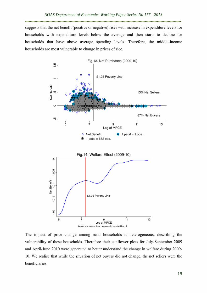
19

suggests that the net benefit (positive or negative) rises with increase in expenditure levels for

households with expenditure levels below the average and then starts to decline for

households that have above average spending levels. Therefore, the middle-income

households are most vulnerable to change in prices of rice.

The impact of price change among rural households is heterogeneous, describing the

vulnerability of these households. Therefore their sunflower plots for July-September 2009

and April-June 2010 were generated to better understand the change in welfare during 2009-

10. We realise that while the situation of net buyers did not change, the net sellers were the

beneficiaries.


20

The heterogeneity in net benefit pattern for rural agricultural labour increased over the year.

The average of positive net benefit increased from 0.12 to 0.17 with the standard deviation

also increasing. Thus, implying increased heterogeneity in welfare. Similar, to the studies on

Mexico37 and Thailand38 we were unable to establish a pattern between welfare generated and

expenditure. It is important to note that the majority of the households in this category are net

buyers who stand to lose from increased prices. The ones who stand to win are subsistence

producers, who cultivate on small farms for consumption purposes and also work as casual

agricultural labour on other farms.

There was a marginal rise (0.09 to 0.12) in welfare for net sellers in the rural agrarian

household category. 46% of these households are net producers and 43% are net sellers. Only

3% grow rice for subsistence purposes. We expected this group to observe a higher average

welfare, as this category includes the rice farmers. A possible reason behind such low net

benefit figures could be that the complete benefit of rising prices did not trickle down to the

producers.

Fig.14 estimates the regression function from fig.13. The regression line is below the x-axis,

therefore on average households stand to lose from higher rice prices irrespective of how

much they spend. For example, for a household with average monthly per capita expenditure

of Rs.1100, a 1% increase in the price of rice will create negative impact of 0.01% (approx.).

But as the curve is upward sloping, the negative impact is more likely to decrease with a rise

in expenditure levels. The curve dips for the middle-income group as these households are

based in urban areas and as the frequency of them being a producer of rice is low. Thus, price

change affects these middle-income households more than the households with higher or

lower expenditure levels39. The net welfare effect for rural and urban areas is presented

below. There exists great diversity in pattern and scale across these households. On average

the welfare impact of increase in price of rice is negative. The only exceptions are the rural

agrarian households, as they are net sellers of rice. However, even this curve (fig.17) is

downward sloping, meaning the benefit declines with increase in expenditure, implying that

most rice producers are small-scale farmers. For the rest of the households the trend is similar

where the poorer the household the more they stand to lose from price rise.

37 Davila (2010) 38 Deaton (1989) 39 Refer to figure3 for the gap between the dash curves from 7.8<lmpce <8.5.


21

The curve for urban households is upward sloping. The net benefit curve for rural households

is upward sloping until lmpce equal to 7, after which is does not follow a particular pattern.

Apart from the shape of the curve, the second most striking feature of the two curves is their

scale. On average urban households are much worse off than their rural counterparts.


22

f) Welfare Analysis in the Absence of the Ban on Rice Exports

We know predict the quarterly net benefit values if the export ban was not implemented and

if the prices in India would have risen in accordance with international rice prices. The fig.18

shows the predicted net benefit for the following quarters; July-September 2007, April-June

2009, July-September 2009 and April-June 2010, and the fig.19 represents the change in net

benefit over the period using the Indian rice prices40.

The poor households would have been much worse off than the richer households, if the

export ban was not implemented. Let us consider the quarter April-June 2008, when the

impact of the crisis was the most. In case of implementation of the export ban, a 1% increase

40 To predict these values consumption and production of rice and expenditure levels for July-September 2009 are kept as constant (as we only have production data for 2009-10). Therefore the predicted net benefit is relative to the consumption and production values of July-September 2009, i.e. how much money the household would require in order to maintain the living standards observed during July-September 2009.


23

in the price of rice would require the poor household to spend 0.013% more of its household

expenditure to enjoy the same living standard; while, the richer households would have to

spend less than 0.005% more. In real terms, if a household’s lmpce is equal to 5; its monthly

per capita expenditure is approximately equal to Rs.150. With a -0.013 net benefit the

household and a 13% rise in price (rice price inflation in India for this quarter) will have to

spend 0.2% more of their current expenditure per person, to maintain their living standard.

But, in the absence of the export ban the same household would have experienced a negative

impact of 0.1 and 150% increase in price (represented by the light blue line in fig.31), which

would require the household to spend 15% more. Net this particular household spent Rs.22

less than it would have if the export ban was not implemented.

We now compare actual and predicted net benefit curves for each quarter. If the actual net

benefit is above the predicted curve, the net impact of the ban on rice exports is positive. For

fig.33 shows us the scenario pre-crisis. The Indian consumers were better off than their

international counterparts. The gap between the actual and predict net benefit curve decreases

as the households get richer. This is line with our previous analysis that the poor households

are more vulnerable, while the rich are resilient to price change.


24

By March 2008 the international rice prices had increased by 100% relative to the June 2007

price levels. In India the rice inflation equalled only 11%. The shift in net benefit pattern is

evident in fig.34 as the scale of curves increases drastically for both the scenarios. The gap

between the blue and grey curve has also increased. In the absence of the export ban on

average the households would have to decrease their living standards as the net benefit

declines to -0.1 for poor households. In reality the net benefit did not vary much across

households and was less than -0.2.

In September 2009, the international rice prices increased by 18% in comparison to June

2007 prices, while in India the price rose by 34%. The following year the rice price inflation

equalled 40% in India, while globally the prices increased by 25%. The figures below show

that the price of rice did not fall along the lines of international prices. But the gap between


25

the actual and predicted curves is around -0.01 for households below lmpce equal to 7 and

below -0.005 for households with lmpce above 7.

Conclusion

The impact of changing food prices depends crucially upon whether the household is a net

seller or buyer of food. The results suggest that 78% of the rural households and 96% of the

urban households are net buyers of rice. Thus even though 58% of the Indian labour force

depends on agriculture for their livelihoods, higher prices of rice do not benefit the majority.

However, the welfare generated by the export ban on rice was positive, as it was able to

cushion the Indian population from the adverse effects of the world food crisis of 2007-08.

The net welfare was positive mainly for two reasons: firstly, on average the Indian population

constitutes of net consumers. Secondly, even though the price of rice in India did not fall in


26

line with the international prices after the crisis, the net benefit lost was much lower in

comparison to the impact of a 150% increase in rice prices.

In terms of identifying the vulnerable groups, the results suggest that the labour class in both

urban and rural areas was affected the most, as they belong to the bottom of the pyramid. On

average urban poor are worse off as they do not produce for subsistence purpose. Thus

policymakers need to pay special focus to this group when considering the impact of

agriculture pricing policies.

The extent of impact on the urban middle class is relatively higher than the households with

expenditure levels around them, as the frequency of them being a net producer is very low.

But these households are more resilient to the change in price as their budget share of rice is

lower compared to the rural households.

Compared to Thailand and Mexico where the middle-income households were the

beneficiaries of increased price of rice and maize respectively, in India this is not the case.

Results suggest this is because rice-producing farmers in India are mainly poor smallholder

farmers. 46% of the rural households self-employed in agriculture are rice producers and 43%

are sellers. Therefore, not many households in this category produce for subsistence

purposes. It is observed that price rise does not only benefit a few large rich farmers but the

group as a whole, with the exception of households below lmpce of 5.8, who belong to the

OBC and Scheduled Tribe caste.

Also, the welfare generated for rural agrarian households was not as high as we expected,

implying that the full benefit of higher prices was not transferred to the farmers. One of the

reasons for the world food crisis was the soaring price of oil. The oil subsidies provided by

the government did not let the cost transfer to the consumers. However, in the light of the

recent policy decisions41 of the Indian government to reduce its oil subsidies, the price of

staples may rise due to the increase in cost of production. However, this rise in price will not

reach the producers who are benefited from the increase in price, creating a lose-lose

situation for both the consumers and the producers.

It is important to note the rice prices in India were contained due to the prevailing

administrative reforms made by the Indian government since independence. Implementation

of the export ban of rice was possible due to existing mechanisms. To a large extent the

excessive government intervention in the sector has had a positive effect on the consumers.

However, the increasing price of rice in 2009-10 while the international rice prices were

41 Financial Times (September 2012)


27

declining indicate that their exist problems more specific to the domestic economy which

require the governments attention, such as the public distribution system, storage facilities

and reduction in oil subsidies. Thus, the results suggest considerable attention may be needed

to protect the vulnerable groups identified.

Appendix

A1. Non-Parametric Estimation of Density and Regressions

A brief description of density estimation and regression is given below to explain the

techniques used for the purpose of the paper.

Similar to Deaton I have used ‘kernel’ estimators. The kernel is a continuous, bounded ad

symmetric function K which integrates to unity. Kernel estimators can be used for both

density and regression function estimation. This approach allows us to set a bandwidth, i.e.,

distance between observations; which determines the contribution of the observations to the

average at each point.

Sliding a moving band along the x-axis, and counting the number of observations that fall

into the bandwidth construct figures 2 and 3. The count is then divided by the number of

observations to estimate the density at a given point. In case the bandwidth is wide the curve

becomes really smooth and curve loses the details of the underlying data. At the same time if

the bandwidth is narrow, the curve is a series of spikes, indicating individual observations.

The advantage of the technique used here is that the data are allowed to choose the shape of

the function is not a model structure specified a priori that forces the points to lie along a

straight line, or along a low-order polynomial.

For example, if we take a kernel estimator and set the bandwidth at 0.25, and at each value of

log of monthly per capita expenditure (lmpce) to calculate the average budget share of rice

for households whose lmpce is within the 0.25 bandwidth. If we decrease the bandwidth by

0.05, the weighted average will give greater weightage to households whose lmpce value is

within 0.20 distance of the value of lmpce being considered.

Formally, the estimate of the regression corresponding to a point X, , say, is

(A1)


28

where Xi and Yi are the x and y values for observation i. The (nonnegative) weights wi will

be zero for Xi which are not within the bandwidth. Although it is also possible to allow all

observations to contribute, but this decreases the weights as the distance between X and Xi

increases.

The equation A1 is a kernel estimator when the weights take the specific form

(A2)

here Kh is the kernel, and h is the bandwidth. Kh is a symmetric monotone decreasing

function that integrates to unity over the range of its argument. K determines the shape of the

kernel weights, whereas the size of the weights is parameterized by h, the bandwidth42. A

commonly used kernel function43, also used here is of parabolic shape called the

Epanechnikov kernel, which is defined by the equation

(A3)

where I is an indicator function, such that I = 1 if X and Xi are within the bandwidth (h) of

one another44. If the X and Xi are not within h, I = 0. The 3/4h is not relevant for calculating

the weights in the equation A2, but it is required to ensure that the integral of Kh(X-Xi) is of

unit value45.

For example, we are interested in estimating the statistical Engel Curve, the average

expenditure for food given a certain level of income. The kernel weights depend on the

values of the X-observations through the density estimate.

The formulae A1, 2 and 3 are used for all the non-parametric regressions used in the main

text, and illustrated in Figs. 4, 17, 18, 27-36 and A6. In Figs. 4 and 26, the dependent variable

y is either the rice share or the net consumption ratio of rice. For figs. 17 and 18, where the

probabilities are estimated, the dependent variable is either one or zero depending on whether

the household does or does not grow and sell rice. All graphs (except for fig.1.) were

42 Hardle (1990) 43 The choice of the smoothing parameter/bandwidth, h, is theoretically more crucial than choice of a kernel function. Most of the asymptotic optimality results of kernel estimation stem from the bandwidth being chosen optimally, that is, to minimize the mean square error. (Budd, 1993, p.601) 44 Deaton (1989) 45 Budd (1993), p.601


29

generated in Stata12. With the exception of few graphs the bandwidth used were defaults

used by Stata.

Where d is an indicator variable that equals 1 if y < C i.e. the observation is uncensored and is equal

to 0 if y= C, i.e. the observation is censored.

The expected value of a censored variable is

Where

We use the tobit model for censored normal regression and use household characteristics are

control variables. After generating the yhat we use the correlate function to see how well related is

yhat to the home production values.


30

A3. Sunflower Plots

02

04

06

08

0R

ice

Sh

are

%

4 6 8 10 12 14Log of MPCE

kernel = epanechnikov, degree = 0, bandwidth = .17

Fig.A1. Example of Scatter Plot

02

04

06

08

0R

ice

Sh

are

%

5 7 9 11 13Log of MPCE

rice share% 1 petal = 1 obs.1 petal = 301 obs.

Fig. A2. Example of Sunflower Plot


31

The sunflower plot is constructed by defining a net of squares covering the (X, Y) space and counting

the number of observations that fall into the disjoint squares. The number of spikes in the hexagon

shaped “sunflower blossom” equal to the number of petals in the sunflower. The petals correspond

to the number of observations in the square around the sunflower. That is, it shows the empirical

distribution of the underlying data. The sunflower plot shows the concentration of the data around

an increasing band of densely packed blossoms or the hexagon46.

Scatter plots of the entire data is very unclear and does not show the areas where the data is

concentrated, due to overstriking of plot symbol47. It is thus desirable to have a technique that

allows us to see the areas where the data is concentrated. The sunflower plot allows us to do so. The

graphs given below map the budget share of rice and the log of monthly per capita expenditure

(lmpce) for the whole dataset (both rounds). When we compare the local polynomial smooth graph,

which is essentially a scatter plot of the two variables we are only able to see the various points

where the data is observed. We are also able to the see the regression line cuts the area mapped in

the graph in the lower half of the green shaded area, indicating that majority of the observations are

in the lower half of the green shaded area. However, when we look at the sunflower plot we can see

that the regions where the data is concentrated. This allows us to understand the distribution in a

more comprehensive manner. The blue circles depict the individual observations at their exact

location when there are less than 3 observations per bin. Light sunflowers are blue and represent

one observation for each petal. Dark sunflowers are grey in colour and represent 301 observations

per petal. This graph not only shows us the density distribution of the observations, but also allows

us to determine the number of observations in a particular region with great precision48.

Through this graph we can thus conclude that the budget share of rice as a percentage of the

expenditure is concentrated around 20% for households with lmpce between 6 and 8. The

sunflower plot also allows us to see the diversity in consumption patterns for households at different

expenditure levels. Below the average lmpce levels (7.03) the households are more diverse in the

patterns of consumption of rise. The rice share percentage is generally below 40%. For lmpce levels

over 8 the rice share percentage drops by half, mostly below 20%. The density of the graph also

increases and is generally consistent in terms of the colour. Thus we conclude that the households

below the lmpce levels of 7 (mean) are more vulnerable to the change in price of rice as their budget

46 Hardle (1990) 47 Dupont and Plummer(2005)p.372 48 Dupont and Plummer(2010)p.375


32

share of rice is more diverse , ranging between 0.004% to 80%. The richer households are fairly

resilient to the change in price.

References

1. Barrett And Dorosh(1996), “Farmers' Welfare And Changing Food Prices: Nonparametric

Evidence From Rice In Madagascar”, American Journal Of Agricultural Economics, Vol. 78,

No. 3 (Aug., 1996), Pp. 656-669 Published

2. Budd, John W. (1993), “Changing Food Prices And Rural Welfare: A Nonparametric

Examination Of The Côte D'ivoire”, Economic Development And Cultural Change, Vol. 41,

No. 3 (Apr., 1993), p.587-603

3. Chen and Ravallion (2010), “The Developing World is Poorer than we Thought, but no Less

Successful in the Fight Against Poverty,” Quarterly Journal of Economics, 2010, Vol. 125.

Issue 4, pp. 1577-1625

4. Dávila, Osiel González (2010), “Food Security And Poverty In Mexico: The Impact Of

Higher Global Food Prices”, Springer

5. Deaton, A. (1989). “Rice Prices And Income Distribution In Thailand: A Non-Parametric

Analysis.” Economic Journal, 99(395), Pp. 1-37.

6. Deaton, A. (1997). “The Analysis Of Household Surveys. A Microeconometric Approach To

Development Policy”, The World Bank And Johns Hopkins University Press, Baltimore And

Washington Dc.

7. FAO (2002), “Sustainable Rice Production For Food Security, Part Ii - Rice In World Trade,

Status Of The World Rice Market In 2002 By- C. Calpe”

8. FAO (2009), “High Food Prices And The Food Crisis - Experiences And Lessons Learned”

9. Financial Times (September 2012), “India Cuts Fuel Subsidies To Curb Deficit”

Http://Www.Ft.Com/Cms/S/0/15e495a0-Fdbc-11e1-9901-

00144feabdc0.Html#Axzz26eboixq4

10. Ghosh and Raychaudhuri (N.D), “ Impact Of Price Change On Supply And Demand For Rice

In Andhra Pradesh And West Bengal”

11. Hardle, W. (1990), “Applied Nonparametric Regression”, Econometric Society Monographs

No. 19, Cambridge University Press

12. Ifpri (2010), “Reflections On The Global Food Crisis: How Did It Happen? How Has It Hurt?

And How Can We Prevent The Next One? “

Indian Economic Survey (2011-12)

13. Jain Et Al (2012), “Caste In A Different Mould: Understanding The Discrimination”


33

14. Lind And Frandsen (2000), “Estimating Food Demand Behaviour: The Case Of India”

15. Lipton M. (1987), “The Limits Of Price Policy For Agriculture: Which Way Now?”,

Development Policy Review, 5.

16. Lipton, M. (1986) "Limits Of Price Policy For Agriculture: Which Way For The World

Bank?" Develop. Policy Rev. 5:197-215.

17. Mellor, John .W (1976), “The New Economics Of Growth: A Strategy For India And The

Developing World”, Cornell University Press

18. Clarkson, Nancy & Kulkarni, Kishore G. (n.d), “Effects Of India’s Trade Policy On Rice

Production And Exports”

19. National Statistical Survey Office (NSSO) for the 64th And 66th (Type-1) Consumer

Household Expenditure Survey.

20. Pons, Nathalie (2011), “Food And Prices In India: Impact Of Rising Food Prices On

Welfare”, Centre De Sciences Humaines, Delhi, India

21. Singh, L. Squire, And J. Strauss, "The Basic Model: Theory, Empirical Results And Policy

Conclusions," In Agricultural Household Models: Extensions, Applications And Policy, Ed. I.

Singh, L. Squire, And J. Strauss (Baltimore: Johns Hopkins University Press, 1986).

22. Ministry Of Commerce And Industry, WPI Base Year 2004-05- Source For Indian Prices

23. FAO International Commodity Prices Data Base - Source For World Prices

24. The Economics Times, February 2012http://Articles.Economictimes.Indiatimes.Com/2012-

02-08/News/31037673_1_Minimum-Export-Price-Vijay-Setia-Rice-Exports

25. USDA (2007), “Indian Wheat And Rice Sector Policies And The Implications Of Reform”,

Economic Research Report United States. Dept. Of Agriculture. Economic Research Service

26. WDR (2007), Agriculture For Development, World Development Report 2008. Washington

Dc.

27. World Bank (1994), Adjustment In Africa: Reforms, Results And The Road Ahead. Oxford:

Oxford University Press.

working paper series issn 1753 - 5816 please cite this

Documents