working with the dicom and nifti data standards in r

JSS Journal of Statistical SoftwareOctober 2011, Volume 44, Issue 6. http://www.jstatsoft.org/

Working with the DICOM and NIfTI Data

Standards in R

Brandon WhitcherMango Solutions

Volker J. SchmidLudwig-Maximilians-Universitat Munchen

Andrew ThorntonCardiff University

Abstract

Two packages, oro.dicom and oro.nifti, are provided for the interaction with andmanipulation of medical imaging data that conform to the DICOM standard or ANA-LYZE/NIfTI formats. DICOM data, from a single file or directory tree, may be uploadedinto R using basic data structures: a data frame for the header information and a matrixfor the image data. A list structure is used to organize multiple DICOM files. The S4 classframework is used to develop basic ANALYZE and NIfTI classes, where NIfTI extensionsmay be used to extend the fixed-byte NIfTI header. One example of this, that has beenimplemented, is an XML-based “audit trail” tracking the history of operations applied toa data set. The conversion from DICOM to ANALYZE/NIfTI is straightforward usingthe capabilities of both packages. The S4 classes have been developed to provide a user-friendly interface to the ANALYZE/NIfTI data formats; allowing easy data input, dataoutput, image processing and visualization.

Keywords: export, imaging, import, medical, visualization.

1. Introduction

Medical imaging is well established in both the clinical and research areas with numerousequipment manufacturers supplying a wide variety of modalities. The DICOM (Digital Imag-ing and Communications in Medicine; http://medical.nema.org/) standard was developedfrom earlier standards and released in 1993. It is the data format for clinical imaging equip-ment and a variety of other devices whose complete specification is beyond the scope of thispaper. All major manufacturers of medical imaging equipment (e.g., GE, Siemens, Philips)have so-called DICOM conformance statements that explicitly state how their hardware im-plements DICOM. The DICOM standard provides interoperability across hardware, but wasnot designed to facilitate efficient data manipulation and image processing. Hence, additional

http://www.jstatsoft.org/

http://medical.nema.org/

2 The DICOM and NIfTI Data Standards in R

oro.dicom

create3D, create4D Create multi-dimensional arrays from DICOMheader/image lists.

dicom2analyze, dicom2nifti Convert DICOM objects to ANALYZE orNIfTI objects.

dicomInfo, dicomSeparate Read single or multiple DICOM files into R.dicomTable, writeHeader Construct data frame from DICOM header list

and write to a CSV file.extractHeader, header2matrix,matchHeader

Extract information from DICOM headers.

str2date, str2time Convert DICOM date or time entry into an Robject.

oro.nifti

afni, anlz, nifti Class constructors for AFNI, ANALYZE andNIfTI objects.

as(<obj>, "nifti") Coerce object into class nifti.audit.trail, aux.file, descrip Extract or replace slots in specific header fields.fmri2oro, oro2fmri Convert between fmridata (fmri) and nifti

objects.hotmetal, tim.colors Useful color tables for visualization.image, orthographic, overlay Two-dimensional visualization methods.is.afni, is.anlz, is.nifti Logical checks.readAFNI, readANALYZE, readNIfTI Data input.writeAFNI, writeANALYZE, writeNIfTI Data otuput.

Table 1: List of functions available in oro.dicom and oro.nifti. Functionality around theAFNI data format was recently added to the oro.nifti package. Please visit http://afni.

nimh.nih.gov/afni/ for more information about the AFNI data format.

data formats have been developed over the years to accommodate data analysis and imageprocessing.

The ANALYZE format was developed at the Mayo Clinic (in the 1990s) to store multidi-mensional biomedical images. It is fundamentally different from the DICOM standard sinceit groups all images from a single acquisition (typically three- or four-dimensional) into apair of binary files, one containing header information and one containing the image infor-mation. The DICOM standard groups the header and image information, typically a singletwo-dimensional image, into a single file. Hence, a single acquisition will contain multipleDICOM files but only a pair of ANALYZE files.

The NIfTI format was developed in the early 2000s by the DFWG (Data Format WorkingGroup) in an effort to improve upon the ANALYZE format. The resulting NIfTI-1 formatadheres to the basic header/image combination from the ANALYZE format, but allows thepair of files to be combined into a single file and re-defines the header fields. In addition,NIfTI extensions allow one to store additional information (e.g., key acquisition parameters,experimental design) inside a NIfTI file.

The material presented here provides users with a method of interacting with DICOM, ANA-LYZE and NIfTI files in R (R Development Core Team 2010). Real-world data sets, that are

http://afni.nimh.nih.gov/afni/

http://afni.nimh.nih.gov/afni/

Journal of Statistical Software 3

publicly available, are used to illustrate the basic functionality of the two packages: oro.dicomand oro.nifti. It should be noted that both packages focus on functions for data input/outputand visualization. S4 classes nifti and anlz are provided for further statistical analysis inR without losing contextual information from the original ANALYZE or NIfTI files. Imagesin the metadata-rich DICOM format may be converted to NIfTI semi-automatically using asmuch information from the DICOM files as possible. Basic visualization functions, similar tothose commonly used in the medical imaging community, are provided for nifti and anlz

objects. Additionally, the oro.nifti package allows one to track every operation on a nifti

object in an XML-based audit trail.

The oro.dicom and oro.nifti packages should appeal not only to R package developers, butalso to scientists and researchers who want to interrogate medical imaging data using thestatistical capabilities of R without writing and validating their own basic data input/outputfunctionality. Table 1 lists the key functions for both packages and groups them according tocommon functionality. An example of using statistical methodology in R for the analysis offunctional magnetic resonance imaging (fMRI) data is given in Section 3.7. Packages alreadyavailable on the Comprehensive R Archive Network (CRAN, http://CRAN.R-project.org/)that utilize oro.dicom and oro.nifti include cudaBayesreg (Ferreira da Silva 2010a; Ferreira daSilva 2011), dcemriS4 (Whitcher and Schmid 2011a,b), dpmixsim (Ferreira da Silva 2010b),and RNiftyReg (Clayden 2011).

2. oro.dicom: DICOM data input/output in R

The DICOM “standard” for data acquired using a clinical imaging device is very broad andcomplex. Roughly speaking each DICOM-compliant file is a collection of fields organizedinto two two-byte sequences (group,element) that are represented as hexadecimal numbersand form a tag. The (group,element) combination establishes what type of information isforthcoming in the file. There is no fixed number of bytes for a DICOM header. The final(group,element) tag should be the “pixel data” tag (7FE0,0010), such that all subsequentinformation is related to the image(s).

All attributes in the DICOM standard require different data types for correct representa-tion. These are known as value representations (VRs) in DICOM, which may be encodedexplicitly or implicitly. There are 27 explicit VRs defined in the DICOM standard. Detailedexplanations of these data types are provided in the Section 6.2 (part 5) of the DICOMstandard (http://medical.nema.org/). Internal functions have been written to manipulateeach of the value representations and are beyond the scope of this article. The functionsstr2date and str2time are useful for converting from the DICOM Datetime and Time valuerepresentations to R date and time objects, respectively.

2.1. The DICOM header

Accessing the information stored in a single DICOM file is provided using the dicomInfo

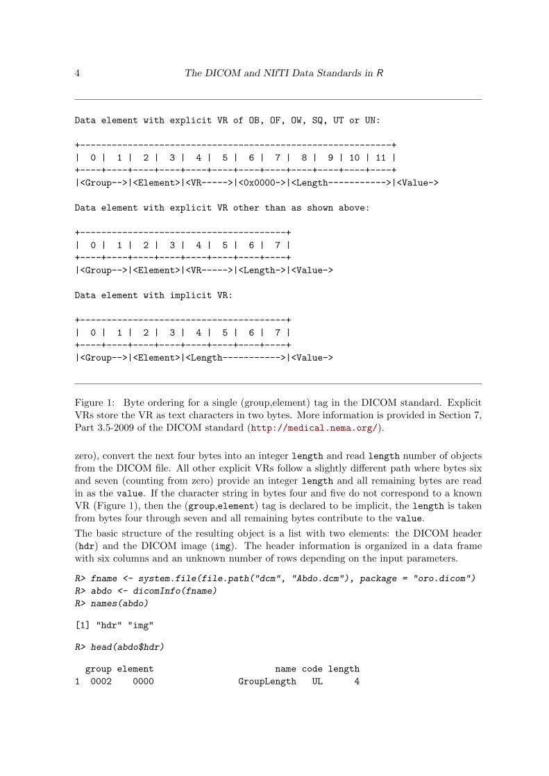
function. The basic structure of a DICOM file is summarized in Figure 1, for both explicitand implicit value representations. The first two bytes represent the group tag and the secondtwo bytes represent the element tag, regardless of the type of VR. The third set of two bytescontains the characters of the VR on which a decision about being implicit or explicit is made.Explicit VRs of type (OB, OF, OW, SQ, UT, UN) skip bytes six and seven (counting from

http://CRAN.R-project.org/



Data element with explicit VR of OB, OF, OW, SQ, UT or UN:

+-----------------------------------------------------------+

| 0 | 1 | 2 | 3 | 4 | 5 | 6 | 7 | 8 | 9 | 10 | 11 |

+----+----+----+----+----+----+----+----+----+----+----+----+

|<Group-->|<Element>|<VR----->|<0x0000->|<Length----------->|<Value->

Data element with explicit VR other than as shown above:

+---------------------------------------+

| 0 | 1 | 2 | 3 | 4 | 5 | 6 | 7 |

+----+----+----+----+----+----+----+----+

|<Group-->|<Element>|<VR----->|<Length->|<Value->

Data element with implicit VR:

+---------------------------------------+

| 0 | 1 | 2 | 3 | 4 | 5 | 6 | 7 |

+----+----+----+----+----+----+----+----+

|<Group-->|<Element>|<Length----------->|<Value->

Figure 1: Byte ordering for a single (group,element) tag in the DICOM standard. ExplicitVRs store the VR as text characters in two bytes. More information is provided in Section 7,Part 3.5-2009 of the DICOM standard (http://medical.nema.org/).

zero), convert the next four bytes into an integer length and read length number of objectsfrom the DICOM file. All other explicit VRs follow a slightly different path where bytes sixand seven (counting from zero) provide an integer length and all remaining bytes are readin as the value. If the character string in bytes four and five do not correspond to a knownVR (Figure 1), then the (group,element) tag is declared to be implicit, the length is takenfrom bytes four through seven and all remaining bytes contribute to the value.

The basic structure of the resulting object is a list with two elements: the DICOM header(hdr) and the DICOM image (img). The header information is organized in a data framewith six columns and an unknown number of rows depending on the input parameters.

R> fname <- system.file(file.path("dcm", "Abdo.dcm"), package = "oro.dicom")

R> abdo <- dicomInfo(fname)

R> names(abdo)

[1] "hdr" "img"

R> head(abdo$hdr)

group element name code length

1 0002 0000 GroupLength UL 4



2 0002 0001 FileMetaInformationVersion OB 2

3 0002 0002 MediaStorageSOPClassUID UI 26

4 0002 0003 MediaStorageSOPInstanceUID UI 38

5 0002 0010 TransferSyntaxUID UI 20

6 0002 0012 ImplementationClassUID UI 16

value sequence

1 166

2 skipped

3 1.2.840.10008.5.1.4.1.1.4

4 1.3.46.670589.11.0.4.1996082307380007

5 1.2.840.10008.1.2.1

6 1.3.46.670589.17

R> tail(abdo$hdr)

group element name code length value sequence

79 0028 0101 BitsStored US 2 12

80 0028 0102 HighBit US 2 11

81 0028 0103 PixelRepresentation US 2 0

82 0028 1050 WindowCenter DS 4 530

83 0028 1051 WindowWidth DS 4 1052

84 7FE0 0010 PixelData OW 131072

The ordering of the rows is identical to the ordering in the original DICOM file. Hence, the firstfive tags in the DICOM header of Abdo.dcm are: GroupLength, FileMetaInformationVersion,MediaStorageSOPClassUID, MediaStorageSOPInstanceUID and TransferSyntaxUID. Thelast five tags in the DICOM header are also shown, with the very last tag indicating the startof the image data for that file and the number of bytes (131072) involved. When additionaltags in the DICOM header information are queried (via extractHeader)

R> extractHeader(abdo$hdr, "BitsAllocated")

[1] 16

R> extractHeader(abdo$hdr, "Rows")

[1] 256

R> extractHeader(abdo$hdr, "Columns")

[1] 256

it is clear that the data are consistent with the header information in terms of the number ofbytes (256 × 256 × (16/8) = 131072).

The first five columns are taken directly from the DICOM header information (group, element,code, length and value) or inferred from that information (name). Note, the (group,element)


values are stored as character strings even though they are hexadecimal numbers. All aspectsof the data frame may be interrogated in R in order to extract relevant information from theDICOM header; e.g., "BitsAllocated" as above. The sequence column is used to keep trackof tags that are embedded in a fixed-length SequenceItems tag or between a SequenceItem-SequenceDelimitationItem pair.

When multiple DICOM files are located in a single directory, or spread across multiple direc-tories, one may use the function dicomSeparate (applied here to the directory hk-40).

R> fname <- system.file("hk-40", package = "oro.dicom")

R> hk40 <- dicomSeparate(fname, verbose = TRUE, counter = 10)

40 files to be processed!

10 files processed...




R> unlist(lapply(hk40, length))

hdr img

40 40

The object associated with dicomSeparate is now a nested set of lists, where the hdr elementis a list of data frames and the img element is a list of matrices. These two lists are associatedin a pairwise sense; i.e., hdr[[1]] is the header information for the image img[[1]]. Defaultparameters recursive = TRUE and pixelData = TRUE (which is actually an input parameterfor dicomInfo) allow the user to search down all possible sub-directories and upload the imagein addition to the header information, respectively. Also, by default all files are treated asDICOM files unless the exclude parameter is set to the unwanted file extension; e.g., exclude= "xml".

The list of DICOM header information across multiple files may be converted to a single dataframe using dicomTable, and written to disc for further analysis; e.g., using write.csv.

R> hk40.info <- dicomTable(hk40$hdr)

R> write.csv(hk40.info, file = "hk40_header.csv")

R> sliceloc.col <- which(hk40$hdr[[1]]$name == "SliceLocation")

R> sliceLocation <- as.numeric(hk40.info[, sliceloc.col])

R> head(sliceLocation)

[1] 160.9315 157.8315 154.7315 151.6315 148.5315 145.4315

R> head(diff(sliceLocation))

[1] -3.1 -3.1 -3.1 -3.1 -3.1 -3.1

R> unique(extractHeader(hk40$hdr, "SliceThickness"))

[1] 3.125


The tag SliceLocation is extracted from the DICOM header information (at the first elementin the list) and processed using the diff function, and should agree with the SliceThicknesstag. Single DICOM fields may also be extracted from the list of DICOM header informationthat contain attributes that are crucial for further image processing; e.g., extracting relevantMR sequences or acquisition timings.

R> head(extractHeader(hk40$hdr, "SliceLocation"))

[1] 160.9315 157.8315 154.7315 151.6315 148.5315 145.4315

R> modality <- extractHeader(hk40$hdr, "Modality", numeric = FALSE)

R> head(matchHeader(modality, "mr"))

[1] TRUE TRUE TRUE TRUE TRUE TRUE

R> (seriesTime <- extractHeader(hk40$hdr, "SeriesTime", numeric = FALSE))

[1] "113751.966000" "113751.966000" "113751.966000" "113751.966000"

[5] "113751.966000" "113751.966000" "113751.966000" "113751.966000"

[9] "113751.966000" "113751.966000" "113751.966000" "113751.966000"

[13] "113751.966000" "113751.966000" "113751.966000" "113751.966000"

[17] "113751.966000" "113751.966000" "113751.966000" "113751.966000"

[21] "113751.966000" "113751.966000" "113751.966000" "113751.966000"

[25] "113751.966000" "113751.966000" "113751.966000" "113751.966000"

[29] "113751.966000" "113751.966000" "113751.966000" "113751.966000"

[33] "113751.966000" "113751.966000" "113751.966000" "113751.966000"

[37] "113751.966000" "113751.966000" "113751.966000" "113751.966000"

R> str2time(seriesTime)

$txt

[1] "11:37:51.96600" "11:37:51.96600" "11:37:51.96600" "11:37:51.96600"

[5] "11:37:51.96600" "11:37:51.96600" "11:37:51.96600" "11:37:51.96600"

[9] "11:37:51.96600" "11:37:51.96600" "11:37:51.96600" "11:37:51.96600"

[13] "11:37:51.96600" "11:37:51.96600" "11:37:51.96600" "11:37:51.96600"

[17] "11:37:51.96600" "11:37:51.96600" "11:37:51.96600" "11:37:51.96600"

[21] "11:37:51.96600" "11:37:51.96600" "11:37:51.96600" "11:37:51.96600"

[25] "11:37:51.96600" "11:37:51.96600" "11:37:51.96600" "11:37:51.96600"

[29] "11:37:51.96600" "11:37:51.96600" "11:37:51.96600" "11:37:51.96600"

[33] "11:37:51.96600" "11:37:51.96600" "11:37:51.96600" "11:37:51.96600"

[37] "11:37:51.96600" "11:37:51.96600" "11:37:51.96600" "11:37:51.96600"

$time

[1] 41871.97 41871.97 41871.97 41871.97 41871.97 41871.97 41871.97

[8] 41871.97 41871.97 41871.97 41871.97 41871.97 41871.97 41871.97

[15] 41871.97 41871.97 41871.97 41871.97 41871.97 41871.97 41871.97

[22] 41871.97 41871.97 41871.97 41871.97 41871.97 41871.97 41871.97

[29] 41871.97 41871.97 41871.97 41871.97 41871.97 41871.97 41871.97

[36] 41871.97 41871.97 41871.97 41871.97 41871.97


Figure 2: Coronal slice of the abdomen viewed in neurological convention (left is right andright is left).

2.2. The DICOM image

Most DICOM files involve a single slice from an acquisition – the image. A notable exception isthe Siemens MOSAIC format (addressed in Section 2.2.1). The oro.dicom package assumes theimage is stored as a flat file of two-byte integers without compression. A variety of additionalimage formats are possible within the DICOM standard; e.g., RGB-colorized, JPEG, JPEGLossless, JPEG 2000 and run-length encoding (RLE). None of these formats are currentlyavailable in oro.dicom. Going back to the Abdo.dcm example, the image is accessed via

R> image(t(abdo$img), col = grey(0:64/64), axes = FALSE, xlab = "",

+ ylab = "")

where the transpose operation is necessary for proper visualization of the image. Figure 2displays a coronal slice through the abdomen from an MRI acquisition. All information fromthe original data acquisition should accompany the image through the DICOM header, andthis information is utilized as much as possible by oro.dicom to simplify the manipulationof DICOM data. As previously shown, this information is easily available to the user bymatching DICOM header fields with valid strings. Note, the function extractHeader assumesthe output should be coerced via as.numeric but this may be disabled setting the inputparameter numeric = FALSE.

R> extractHeader(abdo$hdr, "Manufacturer", numeric = FALSE)

[1] "Philips"


R> extractHeader(abdo$hdr, "RepetitionTime")

[1] 2000

R> extractHeader(abdo$hdr, "EchoTime")

[1] 100

The basic DICOM file structure does not encourage the analysis of multi-dimensional imagingdata (e.g., 3D or 4D) commonly acquired on clinical scanners. Hence, the oro.dicom packagehas been developed to access DICOM files and facilitate their conversion to the NIfTI orANALYZE formats in R. The conversion process requires the oro.nifti package and will beoutlined in Section 4.

Siemens MOSAIC format

Siemens multi-slice EPI (echo planar imaging) data may be collected as a “mosaic” image;i.e., all slices acquired in a single TR (repetition time) frame of a dynamic run are storedin a single DICOM file. The images are stored in an M×N array of images. The functioncreate3D will try to guess the number of images embedded within the single DICOM fileusing the AcquisitionMatrix field. If this doesn’t work, one may enter the (M,N) doubletexplicitly.

R> fname <- system.file(file.path("dcm", "MR-sonata-3D-as-Tile.dcm"),

+ package = "oro.dicom")

R> dcm <- dicomInfo(fname)

R> dim(dcm$img)

[1] 384 384

R> dcmImage <- create3D(dcm, mosaic = TRUE)

R> dim(dcmImage)

[1] 64 64 36

Figure 3a is taken from the raw DICOM file, in mosaic format, and displayed with the defaultmargins in R. Figure 3b is displayed after re-organizing the original DICOM file into a three-dimensional array (it was also converted to the NIfTI format for ease of visualization usingthe overloaded image function in oro.nifti).

3. oro.nifti: NIfTI-1 data input/output in R

Although the industry standard for medical imaging data is DICOM, another format hascome to be heavily used in the image analysis community. The ANALYZE format was orig-inally developed in conjunction with an image processing system (of the same name) at theMayo Foundation. A common version of the format, although not the most recent, is called


(a) (b)

Figure 3: (a) Single MOSAIC image as read in from dicomInfo. (b) Lightbox display ofthree-dimensional array of images after processing via create3D.

ANALYZE 7.5. A copy of the file ANALYZE75.pdf has been included in oro.nifti (accessed viasystem.file("doc/ANALYZE75.pdf", package = "oro.dicom")) since it does not appearto be available from http://www.mayo.edu/ any longer. An ANALYZE 7.5 format image iscomprised of two files, the “.hdr” and “.img” files, that contain information about the acquisi-tion and the acquisition itself, respectively. A more recent adaption of this format is known asNIfTI-1 and is a product of the Data Format Working Group (DFWG) from the Neuroimag-ing Informatics Technology Initiative (NIfTI; http://nifti.nimh.nih.gov/). The NIfTI-1data format is almost identical to the ANALYZE format, but offers a few improvements:

� Merging of the header and image information into one file (.nii).

� Re-organization of the 348-byte fixed header into more relevant categories .

� Possibility of extending the header information.

There are several R packages that also offer input/output functionality for the NIfTI andANALYZE data formats in addition to image analysis capabilities for specific MRI acquisitionsequences; e.g., AnalyzeFMRI (Marchini and Lafaye de Micheaux 2009; Bordier et al. 2011),fmri (Tabelow and Polzehl 2011) and tractor.base (Clayden 2010; Clayden et al. 2011). TheRniftilib package provides access to NIfTI data via the nifticlib library (Granert 2010).

3.1. The NIfTI header

The NIfTI header inherits its structure (348 bytes in length) from the ANALYZE data format.The last four bytes in the NIfTI header correspond to the “magic” field and denote whetheror not the header and image are contained in a single file (magic = "n+1\0") or two separatefiles (magic = "ni1\0"), the latter being identical to the structure of the ANALYZE dataformat. The NIfTI data format added an additional four bytes to allow for “extensions” tothe header. By default these four bytes are set to zero.

http://www.mayo.edu/

http://nifti.nimh.nih.gov/


The first example of reading in, and displaying, medical imaging data in NIfTI formatavg152T1_LR_nifti.nii.gz was obtained from the NIfTI website (http://nifti.nimh.nih.gov/nifti-1/). Successful execution of the commands

R> fname <- system.file(file.path("nifti", "mniLR.nii.gz"),

+ package = "oro.nifti")

R> (mniLR <- readNIfTI(fname))

NIfTI-1 format

Type : niftiAuditTrail

Data Type : 2 (UINT8)

Bits per Pixel : 8

Slice Code : 0 (Unknown)

Intent Code : 0 (None)

Qform Code : 0 (Unknown)

Sform Code : 4 (MNI_152)

Dimension : 91 x 109 x 91

Pixel Dimension : 2 x 2 x 2

Voxel Units : mm

Time Units : sec

R> aux.file(mniLR)

[1] "none "

R> descrip(mniLR)

[1] "FSL3.2beta"

produces an S4 "nifti" object (or "niftiAuditTrail" if the audit trail option is set). Twoaccessor functions are also provided: aux.file and descrip. The former is used to accessthe original name of the file (if it has been provided) and the latter is the name of a validNIfTI header field used to hold a “description” (up to 80 characters in length).

3.2. The NIfTI image

Image information begins at the byte position determined by the voxoffset slot. In a singleNIfTI file (magic = "n+1\0"), this is by default after the first 352 bytes. Header extensionsextend the size of the header and come before the image information leading to a consequentincrease of voxoffset for single NIfTI files. The split NIfTI (magic = "ni1\0") and ANA-LYZE formats contain pairs of files, where the header and image information are separated,and do not have this problem. In this case voxoffset is set to 0.

The image function has been overloaded so that it behaves differently when dealing withmedical image objects (nifti and anlz). The command

R> image(mniLR)

http://nifti.nimh.nih.gov/nifti-1/



(a) (b)

Figure 4: (a) Axial slices of MNI volume mniLR_nifti stored in the neurological convention(right-is-right), but displayed in the radiological convention (right-is-left). (b) Axial slices ofMNI volume mniRL_nifti stored and displayed in the radiological convention.

produces a three-dimensional array of the MNI brain, with the default NIfTI axes, and isdisplayed on a 10×10 grid of images (Figure 4a). The image function for medical imageS4 objects is an attempt to balance minimal user input with enough flexibility to customizethe display when necessary. For example, single slices may be viewed by using the optionplot.type = "single" in conjunction with the option z = to specify the slice.

The second example of reading in and displaying medical imaging data in the NIfTI formatavg152T1_RL_nifti.nii.gz was also obtained from the NIfTI website (http://nifti.nimh.nih.gov/nifti-1/). Successful execution of the commands

R> fname <- system.file(file.path("nifti", "mniRL.nii.gz"),

+ package = "oro.nifti")

R> (mniRL <- readNIfTI(fname))

NIfTI-1 format



Bits per Pixel : 8




Sform Code : 4 (MNI_152)



Voxel Units : mm

Time Units : sec

R> image(mniRL)




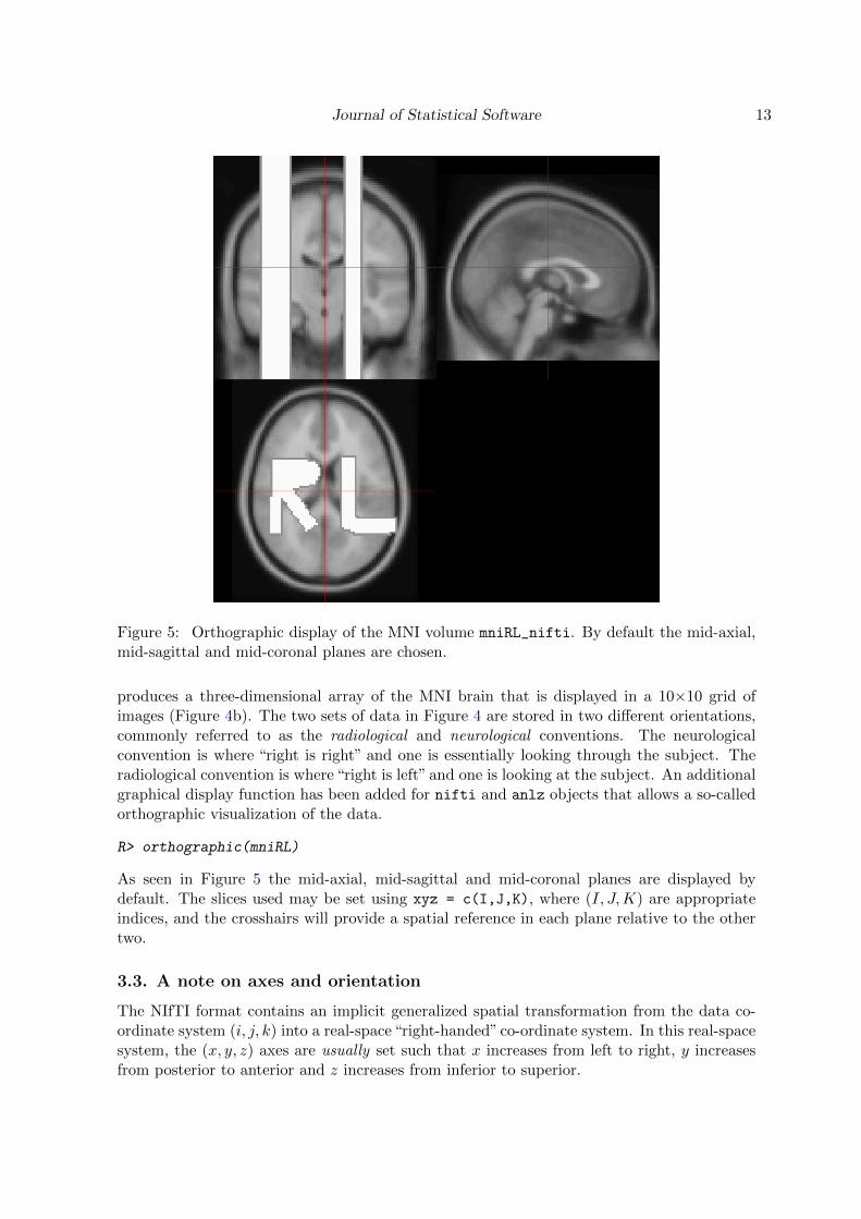
Figure 5: Orthographic display of the MNI volume mniRL_nifti. By default the mid-axial,mid-sagittal and mid-coronal planes are chosen.

produces a three-dimensional array of the MNI brain that is displayed in a 10×10 grid ofimages (Figure 4b). The two sets of data in Figure 4 are stored in two different orientations,commonly referred to as the radiological and neurological conventions. The neurologicalconvention is where “right is right” and one is essentially looking through the subject. Theradiological convention is where “right is left” and one is looking at the subject. An additionalgraphical display function has been added for nifti and anlz objects that allows a so-calledorthographic visualization of the data.

R> orthographic(mniRL)

As seen in Figure 5 the mid-axial, mid-sagittal and mid-coronal planes are displayed bydefault. The slices used may be set using xyz = c(I,J,K), where (I, J,K) are appropriateindices, and the crosshairs will provide a spatial reference in each plane relative to the othertwo.

3.3. A note on axes and orientation

The NIfTI format contains an implicit generalized spatial transformation from the data co-ordinate system (i, j, k) into a real-space “right-handed” co-ordinate system. In this real-spacesystem, the (x, y, z) axes are usually set such that x increases from left to right, y increasesfrom posterior to anterior and z increases from inferior to superior.


At this point in time the oro.nifti package cannot apply an arbitrary transform to the imagingdata into (x, y, z) space – such a transform may require non-integral indices and interpolationsteps. The package does accommodate straightforward transformations of imaging data; e.g.,setting the i-axis to increase from right to left (the neurological convention). Future versionsof oro.nifti will attempt to address more complicated spatial transformations and providefunctionality to display the (x, y, z) axes on orthographic plots.

3.4. NIfTI and ANALYZE data in S4

A major improvement in the oro.nifti package is the fact that standard medical imagingformats are stored in unique classes under the S4 system (Chambers 2008). Essentially, NIfTIand ANALYZE data are stored as multi-dimensional arrays with extra slots created thatcapture the format-specific header information; e.g., for a nifti object

R> slotNames(mniRL)

[1] ".Data" "trail" "extensions" "sizeof_hdr"

[5] "data_type" "db_name" "extents" "session_error"

[9] "regular" "dim_info" "dim_" "intent_p1"

[13] "intent_p2" "intent_p3" "intent_code" "datatype"

[17] "bitpix" "slice_start" "pixdim" "vox_offset"

[21] "scl_slope" "scl_inter" "slice_end" "slice_code"

[25] "xyzt_units" "cal_max" "cal_min" "slice_duration"

[29] "toffset" "glmax" "glmin" "descrip"

[33] "aux_file" "qform_code" "sform_code" "quatern_b"

[37] "quatern_c" "quatern_d" "qoffset_x" "qoffset_y"

[41] "qoffset_z" "srow_x" "srow_y" "srow_z"

[45] "intent_name" "magic" "extender" "reoriented"

R> c(mniRL@cal_min, mniRL@cal_max)

[1] 0 255

R> range(mniRL)

[1] 0 255

R> mniRL@datatype

[1] 2

R> convert.datatype(mniRL@datatype)

[1] "UINT8"

Note, an ANALYZE object has a slightly different set of slots. Slots 4–47 are taken verbatimfrom the definition of the NIfTI format and are read directly from a file. The slot .Data isthe multidimensional array (since class nifti inherits from class array) and the slots trail,extensions and reoriented are used for internal bookkeeping. In the code above we haveaccessed the min/max values of the imaging data using the "cal_min" and "cal_max" slots


and matches a direct interrogation of the .Data slot using the range function. Looking atthe datatype slot provides a numeric code that may be converted into a value that indicatesthe type of byte structure used (in this case an 8-bit or 1-byte unsigned integer).

As introduced in Section 3.1 there are currently only two accessor functions to slots in theNIfTI header (aux.file and descrip) – all other slots are either ignored or used inside offunctions that operate on ANALYZE/NIfTI objects. The NIfTI class also has the abilityto read and write extensions that conform to the NIfTI data format. Customized printingand validity-checking functions are available to the user and every attempt has been made toensure that the information from the multi-dimensional array is in agreement with the headervalues.

The constructor function nifti produces valid NIfTI objects, including a consistent header,from an arbitrary array.

R> n <- 100

R> (random.image <- nifti(array(runif(n * n), c(n, n, 1))))

NIfTI-1 format



Bits per Pixel : 8




Sform Code : 0 (Unknown)



Voxel Units : Unknown

Time Units : Unknown

R> random.image@dim_

[1] 3 100 100 1 1 1 1 1

R> dim(random.image)

[1] 100 100 1

The function writeNIfTI outputs valid NIfTI class files, which can be opened in other medicalimaging software. Files can either be stored as standard .nii files or compressed with gnuzip(default).

R> writeNIfTI(random.image, "random")

R> list.files(pattern = "random")

[1] "random.nii.gz"


R> audit.trail(mniLR)

<audit-trail xmlns="http://www.dcemri.org/namespaces/audit-trail/1.0">

<created>

<workingDirectory>/home/guest/dicom_nifti</workingDirectory>

<filename>/home/bwhitcher/R/x86_64-unknown-linux-gnu-library/2.13/

oro.nifti/nifti/mniLR.nii.gz</filename>

<call>readNIfTI(fname = fname)</call>

<system>

<r-version.version.string>R version 2.13.1 (2011-07-08)

</r-version.version.string>

<date>Sun Aug 21 09:29:36 2011 BST</date>

<user>bwhitcher</user>

<package-version.Version>0.2.7</package-version.Version>

</system>

</created>

</audit-trail>

Figure 6: XML-based audit trail obtained via audit.trail(mniLR).

3.5. The audit trail

Following on from the S4 implementation of both the NIfTI and ANALYZE data formats,the ability to extend the NIfTI data format header is utilized in the oro.nifti package. First,extensions are properly handled when reading and writing NIfTI data. Second, users are al-lowed to add extensions to newly-created NIfTI objects by casting them as niftiExtensionobjects and adding niftiExtensionSection objects to the extensions slot. Third, by de-fault all operations that are performed on a NIfTI object will generate what we call an audittrail that consists of an XML-based log (Temple Lang 2010). Each log entry contains infor-mation not only about the function applied to the NIfTI object, but also various system-levelinformation; e.g., version of R, user name, date, time, etc. When writing NIfTI-class objectsto disk, the XML-based NIfTI extension is converted into plain text and saved using ecode

= 6 to denote plain ASCII text only. The user may control the tracking of data manipulationvia the audit trail using a global option. For example, please use the command

R> options(niftiAuditTrail = FALSE)

to turn off the “audit trail” option in oro.nifti. Figure 6 displays output from the accessorfunction audit.trail(mniLR), the XML-based audit trail that is stored as a NIfTI headerextension.

3.6. Interactive visualization

Basic visualization of nifti and anlz class images can be achieved with any visualizationfor arrays in R. For example, the EBImage package provides functions display and animate

for visualization (Sklyar and Huber 2006; Sklyar et al. 2010). Please note that functions inEBImage expect grey-scale values in the range [0, 1], hence the display of nifti data may beperformed using


R> mniLR.range <- range(mniLR)

R> display((mniLR - min(mniLR))/diff(mniLR.range))

Interactive visualization of multi-dimensional arrays, stored in NIfTI or ANALYZE format, ishowever best performed outside of R at this point in time. Popular viewers, especially for neu-roimaging data, include FSLView (Analysis Group, FMRIB, Oxford 2011), MRIcron (Rorden2011), ITKSnap (Yushkevich et al. 2006), and VolView (Kitware, Inc. 2011). The mritc pack-age provides basic interactive visualization of ANALYZE/NIfTI data using a Tcl/Tk interface(Whitcher et al. 2011; Feng and Tierney 2011).

3.7. An example using functional MRI data

This is an example of reading in, and displaying, a four-dimensional medical imaging data setin NIfTI format filtered_func_data obtained from the FSL evaluation and example datasuite (Analysis Group, FMRIB, Oxford 2008). Successful execution of the commands

R> (ffd <- readNIfTI("filtered_func_data"))

NIfTI-1 format


Data Type : 16 (FLOAT32)

Bits per Pixel : 32




Sform Code : 0 (Unknown)

Dimension : 64 x 64 x 21 x 180

Pixel Dimension : 4 x 4 x 6 x 3

Voxel Units : mm

Time Units : sec

R> image(ffd, zlim = range(ffd) * 0.85)

produces a four-dimensional (4D) array of imaging data that may be displayed in a 5×5 gridof images (Figure 7a). The first three dimensions are spatial locations of the voxel (volumeelement) and the fourth dimension is time for this functional MRI (fMRI) acquisition. As seenfrom the summary of object, there are 21 axial slices of fairly coarse resolution (4×4×6 mm)and reasonable temporal resolution (3 s). Figure 7b depicts the orthographic display ofthe filtered_func_data using the axial plane containing the left-and-right thalamus toapproximately center the crosshair vertically.

R> orthographic(ffd, xyz = c(34, 29, 10), zlim = range(ffd) * 0.85)

Statistical analysis

The R programming environment provides a wide variety of statistical methodology for thequantitative analysis of medical imaging data. For example, fMRI data are typically analyzed


(a)

(b)

Figure 7: (a) Axial slices of the functional MRI data set filtered_func_data from the firstacquisition. (b) Orthographic display of the first volume from the functional MRI data setfiltered_func_data.


0 100 200 300 400 500

−0.

4−

0.2

0.0

0.2

0.4

Acquisition Index

Vis

ual S

timul

us

0 100 200 300 400 500

−0.

4−

0.2

0.0

0.2

0.4

Acquisition Index

Aud

itory

Stim

ulus

Figure 8: Visual (30 seconds on/off) and auditory (45 seconds on/off) stimuli, convolvedwith a parametric haemodynamic response function, used in the GLM-based fMRI analysis.

by applying a multiple linear regression model, commonly referred to in the literature as ageneral linear model (GLM), that utilizes the stimulus experiment to construct the designmatrix. Estimation of the regression coefficients in the GLM produces a statistical image;e.g., Z statistics for a voxel-wise hypothesis test on activation in fMRI experiments (Fristonet al. 1994, 1995).

The 4D volume of imaging data in filtered_func_data was acquired in an experiment witha repetition time TR = 3 s, using both visual and auditory stimuli. The visual stimulus wasapplied using an on/off pattern for a duration of 60 seconds and the auditory stimulus wasapplied using an on/off pattern for a duration of 90 seconds. A parametric haemodynamicresponse function (HRF), with mean µ = 6 and standard deviation σ = 3, is utilized herewhich is similar to the default values in FSL (Smith et al. 2004). We construct the experimen-tal design and HRF in seconds, perform the convolution and then downsample by a factor ofthree in order to obtain columns of the design matrix that match the acquisition of the MRIdata.

R> visual <- rep(c(-0.5, 0.5), each = 30, times = 9)

R> auditory <- rep(c(-0.5, 0.5), each = 45, times = 6)

R> hrf <- c(dgamma(1:15, 4, scale = 1.5))

R> hrf0 <- c(hrf, rep(0, length(visual) - length(hrf)))

R> visual.hrf <- convolve(hrf0, visual)

R> hrf0 <- c(hrf, rep(0, length(auditory) - length(hrf)))

R> auditory.hrf <- convolve(hrf0, auditory)

R> index <- seq(3, 540, by = 3)

R> visual.hrf <- visual.hrf[index]

R> auditory.hrf <- auditory.hrf[index]

Figure 8 depicts the visual and auditory stimuli, convolved with the HRF, in the order of


acquisition. The design matrix is than used in a voxel-wise GLM, where the lsfit functionin R estimates the parameters in the linear regression. At each voxel t statistics and theirassociated p values are computed for the hypothesis test of no effect for each individualstimulus, along with an F statistic for the hypothesis test of no effect of any stimuli using thels.print function.

R> voxel.lsfit <- function(x, thresh) {

+ if (max(x) < thresh) return(rep(NA, 5))

+ output <- lsfit(cbind(visual.hrf, auditory.hrf), x)

+ output.t <- ls.print(output, print.it = FALSE)$coef.table[[1]][2:3,3:4]

+ output.f <- ls.print(output, print.it = FALSE)$summary[3]

+ c(output.t, as.numeric(output.f))

+ }

R> ffd.glm <- apply(ffd, 1:3, voxel.lsfit, thresh = 0.1 * max(ffd))

Given the multidimensional array of output from the GLM fitting procedure, the t statisticsare separated and converted into Z statistics to follow the convention used in FSL. For thepurposes of this example we have not applied any multiple comparisons correction procedureand, instead, use a relatively large threshold of Z > 5 for visualization.

R> dof <- ntim(ffd) - 1

R> Z.visual <- nifti(qnorm(pt(ffd.glm[1, , , ], dof, log.p = TRUE),

+ log.p = TRUE), datatype = 16)

R> Z.auditory <- nifti(qnorm(pt(ffd.glm[2, , , ], dof, log.p = TRUE),

+ log.p = TRUE), datatype = 16)

R> overlay(ffd, ifelse(Z.visual > 5, Z.visual, NA),

+ zlim.x = range(ffd) * 0.85, zlim.y = range(Z.visual, na.rm = TRUE))

R> overlay(ffd, ifelse(Z.auditory > 5, Z.auditory, NA),

+ zlim.x = range(ffd) * 0.85, zlim.y = range(Z.auditory, na.rm = TRUE))

Statistical images in neuroimaging are commonly displayed as an overlay on top of a referenceimage (one of the dynamic acquisitions) in order to provide anatomical context. The overlaycommand in oro.nifti allows one to display the statistical image of voxel-wise activationsoverlayed on one of the original EPI (echo planar imaging) volumes acquired in the fMRIexperiment. The 3D array of Z statistics for the visual and auditory tasks are overlayed onthe original data for “anatomical” reference in Figure 9. The Z statistics that exceed thethreshold appear to match know neuroanatomy, where the visual cortex in the occipital lobeshows activation under the visual stimulus (Figure 9a) and the primary auditory cortex inthe temporal lobe shows activation under the auditory stimulus (Figure 9b).

4. Converting DICOM to NIfTI

The oro.dicom and oro.nifti packages have been specifically designed to use as much infor-mation as possible from the metadata-rich DICOM format and apply that information in theconstruction of the NIfTI data volume. The function dicom2nifti converts a list of DICOMimages into an nifti object, and likewise dicom2analyze converts such a list into an anlz

object.


(a)

(b)

Figure 9: (a) Axial slices of the functional MRI data with the statistical image from thevisual stimulus overlayed. (b) Axial slices of the functional MRI data with the statisticalimage from the auditory stimulus overlayed. Both sets of test statistics were thresholded atZ ≥ 5 for all voxel.


Historically, data conversion from DICOM to NIfTI (or ANALYZE) has been provided outsideof R using one of several standalone software packages: XMedCon (Nolf 2003), FreeSurfer(Athinoula A. Martinos Center for Biomedical Imaging 2011), MRIConvert (Smith 2011).This is by no means an exhaustive list of software packages available for DICOM conversion.In addition there are several other R packages with the ability to process DICOM data: fmri(Tabelow and Polzehl 2011), tractor.base (Clayden 2010; Clayden et al. 2011, part of thetractor project http://code.google.com/p/tractor).

4.1. An example using a single-series data set

Using the 40 images from the hk40 object (previously defined in Section 2.1) it is straightfor-ward to perform DICOM-to-NIfTI conversion using only default settings and plot the resultsin either lightbox or orthographic displays.

R> args(dicom2nifti)

function (dcm, datatype = 4, units = c("mm", "sec"), rescale = FALSE,

reslice = TRUE, qform = TRUE, sform = TRUE, DIM = 3,

descrip = "SeriesDescription", aux.file = NULL, ...)

NULL

R> (hk40n <- dicom2nifti(hk40))

NIfTI-1 format


Data Type : 4 (INT16)

Bits per Pixel : 16



Qform Code : 2 (Aligned_Anat)

Sform Code : 2 (Aligned_Anat)


Pixel Dimension : 1.56 x 1.56 x 3.12

Voxel Units : mm

Time Units : sec

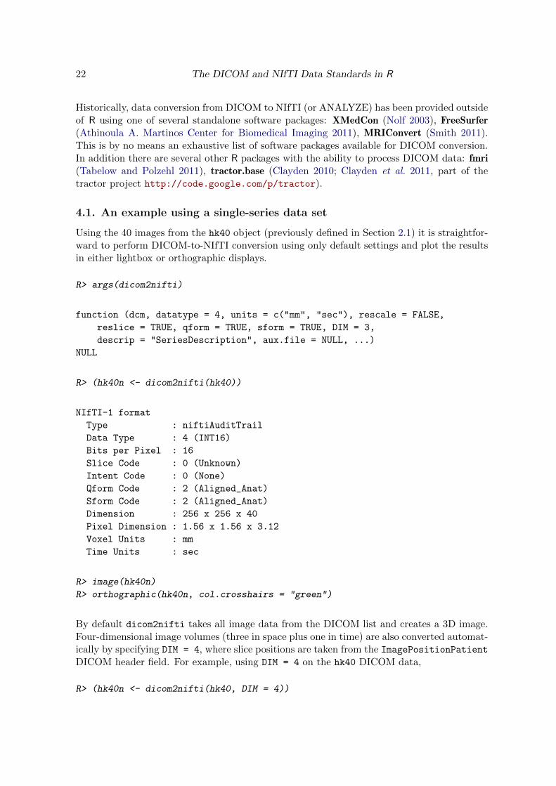
R> image(hk40n)

R> orthographic(hk40n, col.crosshairs = "green")

By default dicom2nifti takes all image data from the DICOM list and creates a 3D image.Four-dimensional image volumes (three in space plus one in time) are also converted automat-ically by specifying DIM = 4, where slice positions are taken from the ImagePositionPatientDICOM header field. For example, using DIM = 4 on the hk40 DICOM data,

R> (hk40n <- dicom2nifti(hk40, DIM = 4))

http://code.google.com/p/tractor


(a)

(b)

Figure 10: (a) Lightbox display of three-dimensional array of images. (b) Orthographicdisplay of the same three-dimensional array (using the default settings for orthographic).


NIfTI-1 format


Data Type : 4 (INT16)

Bits per Pixel : 16



Qform Code : 2 (Aligned_Anat)

Sform Code : 2 (Aligned_Anat)


Pixel Dimension : 1.56 x 1.56 x 3.12

Voxel Units : mm

Time Units : sec

will also produce a three-dimensional volume of images, since the ImagePositionPatient

field is unique for each single slice of the volume.

The functions dicom2nifti and dicom2analyze will fail when the dimensions of the indi-vidual images in the DICOM list do not match. However, they do not check for differentseries numbers or patient IDs so caution should be exercised when scripting automated workflows for DICOM-to-NIfTI conversion. In cases where a DICOM file includes images frommore than one series, the corresponding slices have to be chosen before conversion, usingdicomTable, extractHeader, and matchHeader.

4.2. An example using a multiple-volume data set

The National Biomedical Imaging Archive (NBIA; http://cabig.nci.nih.gov/tools/NCIA)is a searchable, national repository integrating in vivo cancer images with clinical and genomicdata. The NBIA provides the scientific community with public access to DICOM images, im-age markup, annotations, and rich metadata. The multiple MRI sequences processed herewere downloaded from the “RIDER Neuro MRI” collection at http://wiki.nci.nih.gov/

display/CIP/RIDER. A small for loop has been written to operate on a subset of the DI-COM directory structure, where the SeriesInstanceUID DICOM header field is assumed tobe 100% accurate in series differentiation.

R> subject <- "1086100996"

R> DCM <- dicomSeparate(subject, verbose = TRUE, counter = 100)

564 files to be processed!






R> seriesInstanceUID <- extractHeader(DCM$hdr, "SeriesInstanceUID",

+ FALSE)

R> for (uid in unique(seriesInstanceUID)) {

+ index <- which(unlist(lapply(DCM$hdr, function(x) uid %in% x$value)))

http://cabig.nci.nih.gov/tools/NCIA

http://wiki.nci.nih.gov/display/CIP/RIDER

http://wiki.nci.nih.gov/display/CIP/RIDER


+ uid.dcm <- list(hdr = DCM$hdr[index], img = DCM$img[index])

+ patientsName <- extractHeader(uid.dcm$hdr, "PatientsName", FALSE)

+ studyDate <- extractHeader(uid.dcm$hdr, "StudyDate", FALSE)

+ seriesDescription <- extractHeader(uid.dcm$hdr, "SeriesDescription",

+ FALSE)

+ fname <- paste(gsub("[^0-9A-Za-z]", "", unique(c(patientsName,

+ studyDate, seriesDescription))), collapse = "_")

+ cat("## ", fname, fill = TRUE)

+ if (gsub("[^0-9A-Za-z]", "", unique(seriesDescription)) == "axtensor") {

+ D <- 4

+ reslice <- FALSE

+ } else {

+ D <- 3

+ reslice <- TRUE

+ }

+ uid.nifti <- dicom2nifti(uid.dcm, DIM = D, reslice = reslice,

+ descrip = c("PatientID", "SeriesDescription"))

+ writeNIfTI(uid.nifti, fname)

+ }

## 281949_19040720_axtensor

## 281949_19040720_ax30flip

## 281949_19040720_ax15flip

## 281949_19040720_ax25flip

## 281949_19040720_ax20flip

## 281949_19040720_ax10flip

## 281949_19040720_ax5flip

Note, the diffusion tensor imaging (DTI) data axtensor is assumed to be four dimensionaland all other series (the multiple flip-angle acquisitions) are assumed to be three dimensional.There is always a balance between what information should be pre-specified versus what caneasily be extracted from the DICOM headers or images.

5. Conclusion

Medical image analysis depends on the efficient manipulation and conversion of DICOM data.The oro.dicom and oro.nifti packages have been developed to provide the user with a set offunctions that mask as many of the background details as possible while still providing flexibleand robust performance.

The future of medical image analysis in R will benefit from a unified view of the imaging datastandards: DICOM, NIfTI and ANALYZE. The existence of a single package for handlingimaging data formats would facilitate interoperability between the ever increasing number ofR packages devoted to medical image analysis. We do not assume that the data structuresin oro.dicom or oro.nifti are best-suited for this purpose and we welcome an open discussionaround how best to provide this standardization to the end user.


Acknowledgments

The authors would like to thank the National Biomedical Imaging Archive (NBIA), the Na-tional Cancer Institute (NCI), the National Institute of Health (NIH) and all institutions thathave contributed medical imaging data to the public domain. The authors would also like tothank K. Tabelow for providing functionality around the AFNI data format. VS is supportedby the German Research Council (DFG SCHM 2747/1-1).

References

Analysis Group, FMRIB, Oxford (2008). FSL 4.1 FMRIB Software Library. URL http:

//www.fmrib.ox.ac.uk/fsl/fsl/feeds.html.

Analysis Group, FMRIB, Oxford (2011). FSLView v3.1. URL http://fsl.fmrib.ox.ac.

uk/fsl/fslview/.

Athinoula A Martinos Center for Biomedical Imaging (2011). FreeSurfer v5.1.0. URLhttp://surfer.nmr.mgh.harvard.edu/.

Bordier C, Dojat M, Lafaye de Micheaux P (2011). “Temporal and Spatial IndependentComponent Analysis for fMRI Data Sets Embedded in the AnalyzeFMRI R Package.”44(9), 1–24. URL http://www.jstatsoft.org/v44/i09/.

Chambers JM (2008). Software for Data Analysis: Programming in R. Springer-Verlag, NewYork.

Clayden J (2010). tractor.base: A Package for Reading, Manipulating and VisualisingMagnetic Resonance Images. R package version 1.5.0, URL http://CRAN.R-project.org/

package=tractor.base.

Clayden J (2011). RNiftyReg: Medical Image Registration Using the NiftyReg Library.R package version 0.3.1, based on original code by Marc Modat and Pankaj Daga, URLhttp://CRAN.R-project.org/package=RNiftyReg.

Clayden JD, Munoz Maniega S, Storkey AJ, King MD, Bastin ME, Clark CA (2011). “Trac-toR: Magnetic Resonance Imaging and Tractography with R.” Journal of Statistical Soft-ware, 44(8), 1–18. URL http://www.jstatsoft.org/v44/i08/.

Feng D, Tierney L (2011). mritc: MRI Tissue Classification. R package version 0.3-3, URLhttp://CRAN.R-project.org/package=mritc.

Ferreira da Silva A (2010a). cudaBayesreg: CUDA Parallel Implementation of a BayesianMultilevel Model for fMRI Data Analysis. R package version 0.3-9, URL http://CRAN.

R-project.org/package=cudaBayesreg.

Ferreira da Silva A (2010b). dpmixsim: Dirichlet Process Mixture Model Simulation for Clus-tering and Image Segmentation. R package version 0.0-5, URL http://CRAN.R-project.

org/package=dpmixsim.

http://www.fmrib.ox.ac.uk/fsl/fsl/feeds.html

http://www.fmrib.ox.ac.uk/fsl/fsl/feeds.html

http://fsl.fmrib.ox.ac.uk/fsl/fslview/

http://fsl.fmrib.ox.ac.uk/fsl/fslview/

http://surfer.nmr.mgh.harvard.edu/

http://www.jstatsoft.org/v44/i09/

http://CRAN.R-project.org/package=tractor.base

http://CRAN.R-project.org/package=tractor.base

http://CRAN.R-project.org/package=RNiftyReg


http://CRAN.R-project.org/package=mritc

http://CRAN.R-project.org/package=cudaBayesreg

http://CRAN.R-project.org/package=cudaBayesreg

http://CRAN.R-project.org/package=dpmixsim

http://CRAN.R-project.org/package=dpmixsim


Ferreira da Silva AR (2011). “cudaBayesreg: Parallel Implementation of a Bayesian MultilevelModel for fMRI Data Analysis.” Journal of Statistical Software, 44(4), 1–24. URL http:

//www.jstatsoft.org/v44/i04/.

Friston KJ, Holmes AP, Poline JB, Grasby PM, Williams SCR, Frackowiak RSJ, Turner R(1995). “Analysis of fMRI Time Series Revisited.” NeuroImage, 2, 45–53.

Friston KJ, Holmes AP, Worsley KJ, Poline JP, Frith CD, Frackowiak RSJ (1994). “StatisticalParametric Maps in Functional Imaging: A General Linear Approach.” Human BrainMapping, 2, 189–210.

Granert O (2010). Rniftilib: R Interface to nifticlib (V1.1.0). R package version 0.0-29,URL http://CRAN.R-project.org/package=Rniftilib.

Kitware, Inc (2011). VolView 3.4. URL http://www.kitware.com/products/volview.

html.

Marchini JL, Lafaye de Micheaux P (2009). AnalyzeFMRI: Functions for Analysis of fMRIDatasets Stored in the ANALYZE or NIFTI Format. R package version 1.1-11, URL http:

//CRAN.R-project.org/package=AnalyzeFMRI.

Nolf E (2003). “XMedCon – An Open-Source Medical Image Conversion Toolkit.” EuropeanJournal of Nuclear Medicine, 30(Suppl. 2), S246. URL http://xmedcon.sourceforge.

net/.

R Development Core Team (2010). R: A Language and Environment for Statistical Computing.R Foundation for Statistical Computing, Vienna, Austria. ISBN 3-900051-07-0, URL http:

//www.R-project.org/.

Rorden C (2011). MRIcro Software Guide. Version 1.40 build 1, URL http://www.MRIcro.

com/.

Sklyar O, Huber W (2006). “Image Analysis for Microscopy Screens.” R News, 6(5), 12–16.URL http://CRAN.R-project.org/doc/Rnews/.

Sklyar O, Pau G, Smith M, Huber W (2010). EBImage: Image Processing Toolbox for R.R package version 3.5.5, URL http://www.Bioconductor.org/packages/release/bioc/

html/EBImage.html.

Smith J (2011). MRIConvert: A Nifty DICOM File Converter. Lewis Center for Neuroimag-ing, University of Oregon, URL http://lcni.uoregon.edu/~jolinda/MRIConvert/.

Smith SM, Jenkinson M, Woolrich MW, Beckmann CF, Behrens TEJ, Johansen-Berg H,Bannister PR, Luca MD, Drobnjak I, Flitney DE, Niazy R, Saunders J, Vickers J, ZhangY, Stefano ND, Brady JM, Matthews PM (2004). “Advances in Functional and StructuralMR Image Analysis and Implementation as FSL.” NeuroImage, 23(Supplement 1), 208–219.

Tabelow K, Polzehl J (2011). “Statistical Parametric Maps for Functional MRI Experimentsin R: The Package fmri.” Journal of Statistical Software, 44(11), 1–21. URL http://www.

jstatsoft.org/v44/i11/.



http://CRAN.R-project.org/package=Rniftilib

http://www.kitware.com/products/volview.html

http://www.kitware.com/products/volview.html

http://CRAN.R-project.org/package=AnalyzeFMRI

http://CRAN.R-project.org/package=AnalyzeFMRI

http://xmedcon.sourceforge.net/

http://xmedcon.sourceforge.net/

http://www.R-project.org/

http://www.R-project.org/

http://www.MRIcro.com/

http://www.MRIcro.com/

http://CRAN.R-project.org/doc/Rnews/

http://www.Bioconductor.org/packages/release/bioc/html/EBImage.html

http://www.Bioconductor.org/packages/release/bioc/html/EBImage.html

http://lcni.uoregon.edu/~jolinda/MRIConvert/




Temple Lang D (2010). XML: Tools for Parsing and Generating XML within R and S-PLUS.R package version 3.1-0, URL http://CRAN.R-project.org/package=XML.

Whitcher B, Schmid VJ (2011a). dcemriS4: A Package for Medical Image Analysis. Rpackage version 0.43, URL http://CRAN.R-project.org/package=dcemriS4.

Whitcher B, Schmid VJ (2011b). “Quantitative Analysis of Dynamic Contrast-Enhanced andDiffusion-Weighted Magnetic Resonance Imaging for Oncology in R.” Journal of StatisticalSoftware, 44(5), 1–29. URL http://www.jstatsoft.org/v44/i05/.

Whitcher B, Schmid VJ, Thornton A (2011). “Working with the DICOM and NIfTI Data Stan-dards in R.” Journal of Statistical Software, 44(6), 1–28. URL http://www.jstatsoft.

org/v44/i06/.

Yushkevich PA, Piven J, Cody Hazlett H, Gimpel Smith R, Ho S, Gee JC, Gerig G (2006).“User-Guided 3D Active Contour Segmentation of Anatomical Structures: SignificantlyImproved Efficiency and Reliability.” Neuroimage, 31(3), 1116–1128.

Affiliation:

Brandon WhitcherMango SolutionsOffice 202, Second Floor14 Greville StreetLondon EC1N 8SB, United KingdomE-mail: [email protected]: http://www2.imperial.ac.uk/~bwhitche/,

http://rigorousanalytics.blogspot.com/

Volker J. SchmidBioimaging GroupDepartment of StatisticsLudwig-Maximilians-Universitat Munchen80539 Munchen, GermanyE-mail: [email protected]: http://volkerschmid.de/

Andrew ThorntonCardiff University School of Medicine

http://CRAN.R-project.org/package=XML

http://CRAN.R-project.org/package=dcemriS4




mailto:[email protected]

http://www2.imperial.ac.uk/~bwhitche/

http://rigorousanalytics.blogspot.com/


http://volkerschmid.de/


Heath ParkCardiff CF14 4XN, United KingdomE-mail: [email protected]

Journal of Statistical Software http://www.jstatsoft.org/

published by the American Statistical Association http://www.amstat.org/

Volume 44, Issue 6 Submitted: 2010-10-25October 2011 Accepted: 2011-06-07


http://www.jstatsoft.org/

http://www.amstat.org/

working with the dicom and nifti data standards in r

Documents