workpackage 5 ‘benefit of the doubt’ composite indicators

Workpackage 5

‘Benefit of the doubt’ composite indicators Deliverable 5.3

2008

II

KEI-WP5-D5.3

List of contributors: Laurens Cherchye, Willem Moesen, Nicky Rogge, Tom Van Puyenbroeck Main responsibility: Laurens Cherchye, Willem Moesen, Nicky Rogge, Tom Van Puyenbroeck CIS8–CT–2004–502529 KEI

The project is supported by European Commission by funding from the Sixth Framework Programme for Research. http://europa.eu.int/comm/research/index_en.cfm http://europa.eu.int/comm/research/fp6/ssp/kei_en.htm http://www.cordis.lu/citizens/kick_off3.htm http://kei.publicstatistics.net/

III

© http://kei.publicstatistics.net - 2008

Preface Despite their increasing use, composite indicators remain controversial. The undesirable dependence of countries’ rankings on the preliminary normalization stage, and the disagreement among experts/stakeholders on the specific weighting scheme used to aggregate sub-indicators, have been invoked to undermine the credibility of composite indicators. Data Envelopment Analysis may be instrumental in overcoming these limitations. One part of its appeal in the composite indicator context stems from its invariance to measurement units, which entails that a normalization stage can be skipped. Secondly, it fills the informational problem about the ‘right’ set of weights by generating flexible ‘benefit of the doubt’-weights for each evaluated country. The ease of interpretation is a third advantage of the specific model that is the main focus of this paper. In sum, the method may help to neutralize some recurring sources of criticism on composite indicators, allowing one to shift the focus to other, and perhaps more essential stages of their construction. This paper is an abridged version of the paper “An introduction to ‘benefit of the doubt’ composite indicators published in Social Indicators Research. It was presented at the Q2006 Conference, Cardiff, April, 2006 in the KEI session. The authors wish to thank the other members of the KEI-project (contract n° 502529, European Commission’s Sixth Framework Programme), and in particular Prof. Dr. Ralf Münnich for the organisation of this session as well as the cooperation during the project. Corresponding author: [email protected]

IV

KEI-WP5-D5.3

Contents Chapter 1 Introduction ............................................................................................................ 1 Chapter 2 Data Envelopment Analysis and “Benefit of the Doubt”-weighting ..................... 4 Chapter 3 Sub-Indicator Share Restrictions ............................................................................ 8 Chapter 4 Dealing with Imprecise Data ................................................................................ 12 Chapter 5 Concluding remarks ............................................................................................. 15

1


Chapter 1 Introduction

The mere variety of composite indicators reflects their recognition as tools for policy evaluation and communication. Yet despite their increasing prevalence, composite indicators remain the subject of controversy. The lack of a standard construction methodology, and particularly the inescapable subjectivity involved in their construction, are invoked by opponents to undermine their credibility. Subjective choices are indeed pervasive when answering the many questions bound up with a composite indicator (see Booysen, 2002): what is the overall phenomenon one purports to summarize; which sub-indicators should be included; how should they be aggregated; how to deal with missing or low quality data; to what extent can one assess how country rankings are influenced by all the foregoing questions, etc.? Some of these problems are fundamental, as they relate to the substantive content of any composite indicator: is it just a contrivance to summarize several data dimensions, or does one really aspire to summarize a complex, multi-faceted phenomenon such as human development, social inclusion, the knowledge-based economy, competitiveness,…? We will take it here that summarizing is one of its two essential purposes, the other one being the idea of comparing several countries (or the evolution of a country over time, and the like). We will also take it that composite indicators bear, although limitedly, on public debate. Because they are so easy to use as communication tools, they inevitably do show up in media headlines and in press releases of well-respected international organizations, so at least increasing awareness of specific issues in society. In such cases, they often have an hit-parade appearance. And most probably, this feature only aggravates uneasy feelings about composite indicators in scholarly circles. We immediately turn to the simplest form, in which the composite index is formulated as a weighted average of the individual indicators:

∑=

=m

i

nicicc ywCI

1,, . (1)

with cCI the composite index for country j, n

icy , the (possibly normalized) value for country j on indicator i (i = 1,…m) and iw the weight assigned to indicator i. In general, weights are

bounded in that 10 , ≤≤ icw and ∑=

=m

iicw

1, 1. In the construction process, the lack of a

standard methodology is often invoked by opponents to undermine the credibility of the composite indicators. A first typical problem of most CIs is that the sub-indicators are displayed in quite diverse measurement units. This may be problematic in that adding up apples and oranges has to be avoided. In fact, getting rid of measurement units —notably when these differ across dimensions— is one reason why CI practitioners employ normalization methods. However, this doesn’t really solve the problem. A first general remark is that normalization obscures the original purpose of the indicator: one is no longer summarizing the original data, but re-scaled scores, or distances to goalposts, or z-scores, and the like. Evidently, this also bears on the inter-country score comparisons. There is, however, an observation that is still more worrying. Keeping the weighting system fixed, the eventual

2

KEI-WP5-D5.3

rankings still depend on the particular (and so-called ‘preliminary’) normalization option taken. Ebert and Welsch (2004) criticize the dependency of eventual ranks on the normalization/aggregation procedure from a measurement-theoretic point of view. In a well-defined mathematical sense, a composite indicator is not meaningful when the resulting country ordering changes if the original data are transformed in such a way that there informational content is not fundamentally altered. In practice, however, most composite indicators are prone to precisely this deficiency. It is obvious that countries with lower rankings due to a specific normalization procedure may invoke this dependency to question the credibility and the use of composite indicators. Removing the requirement to normalize the data would eliminate this dependency and, thus, an important source of criticism. A second issue relates to the weighting scheme used for aggregating the sub-indicators. Ideally, the sub-indicators should be weighted and combined in a manner reflecting the underlying structure of the evaluated phenomenon. Often, however, it is not at all clear what (‘paternalistic’) judgments to impute, especially since weighting information stemming from stakeholders is often characterized by strong inter-individual disagreements. Equal weighting, which is just a specific case of fixed weighting, is therefore regularly invoked as the standard in virtue of its simplicity (e.g. by Babbie, 1995). Yet, this alleged simplicity is often thoroughly misleading. In the absence of any specific knowledge about the ‘true’ weights, it is even questionable whether any fixed weighting scheme should be applied at all. The essential reason for this is the same as for the normalization issue, namely that country scores and rankings also depend on the specific weighting scheme. In practice, very frequently such fixed weighting schemes favour some countries while harming others. Furthermore, as an alternative for the paternalism bound up with fixed weighting schemes, it may be desirable –notably in the EU-context where this may be a sensitive issue- to take the specificity of each country into account as much as possible. Within this perspective, differential weighting may be desirable, if not necessary, to come to representative CIs. The rest of this text discusses how Data Envelopment Analysis helps to overcome the issues just raised. This approach has already been applied to composite indicators in the context of policy performance assessment. For example, it has been used to gauge countries’ performance with regard to aggregate deprivation (Zaim, Färe and Grosskopf, 2001), to provide an alternative weighting system for the Human Development Index (Mahlberg and Obersteiner, 2001, Despotis, 2005), or as a generalized gauge for Sustainable Development (Cherchye and Kuosmanen, 2006). Especially in the European context, where tensions between the centre and member states may also bear on the precise way by which the latters’ policies are evaluated, the need for a flexible weighting system may be warranted. Indeed, besides academic contributions (e.g.: European Unemployment policy (Storrie and Bjurek, 2000), Social Inclusion policy (Cherchye, Moesen, Van Puyenbroeck, 2004), and Internal Market policy (Cherchye, Lovell, Moesen, Van Puyenbroeck, 2005)), the European Commission itself has used the technique to gauge member states’ performance with regard to the Lisbon objectives (European Commission, 2004, p. 376-378). In this paper, a miniature subset of the Knowledge Based Economy Indicator (KEI), is used to provide illustrative examples. More precisely, out of a dataset containing 94 potential sub-indicators for measuring the drivers, characteristics, and key outputs of a knowledge economy, we selected 7 sub-indicators which we perceived to be intrinsically significant (see Table 1). Specifically, these 7 sub-indicators are (i) Share of ICT sector value added out of total business sector value added (% of total), (ii) Percentage of individuals using the internet for banking (% of individuals), (iii) Percentage of firms who use the internet to interact with public authorities (% of firms), (iv) Pisa reading literacy of 15 year olds (PISA score points), (v) Triadic patent families by priority year per million population (number per million

3


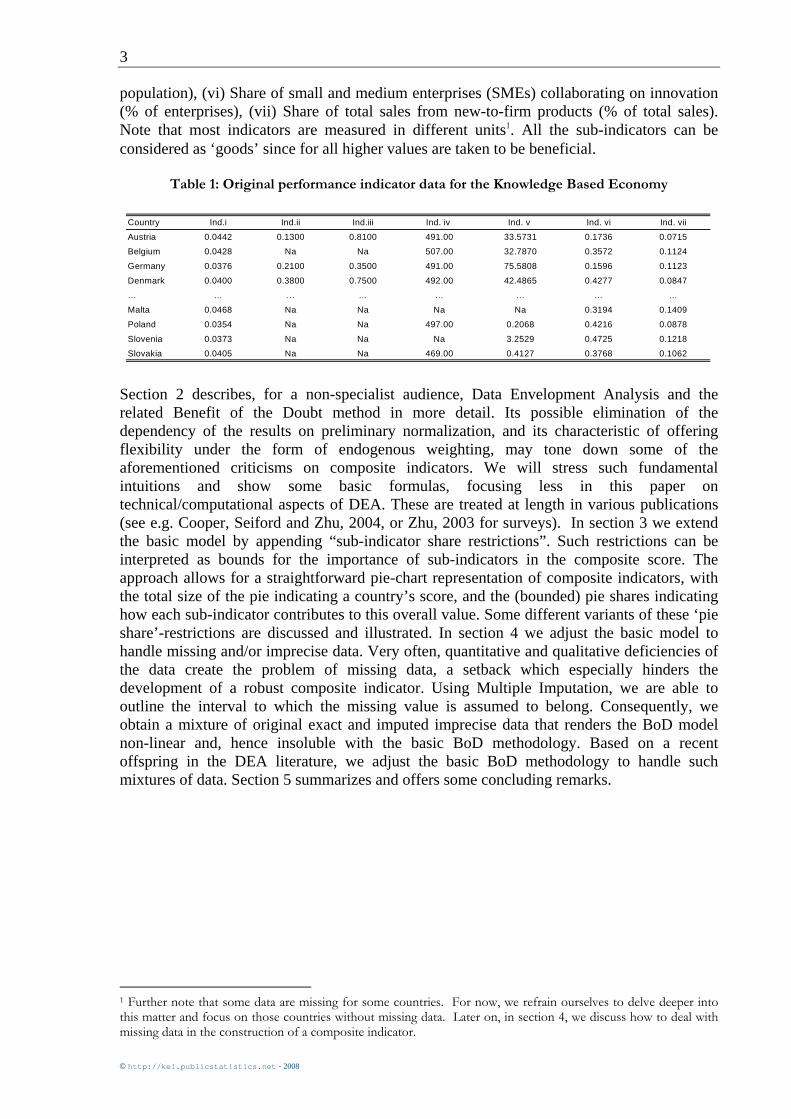
population), (vi) Share of small and medium enterprises (SMEs) collaborating on innovation (% of enterprises), (vii) Share of total sales from new-to-firm products (% of total sales). Note that most indicators are measured in different units1. All the sub-indicators can be considered as ‘goods’ since for all higher values are taken to be beneficial.

Table 1: Original performance indicator data for the Knowledge Based Economy

Section 2 describes, for a non-specialist audience, Data Envelopment Analysis and the related Benefit of the Doubt method in more detail. Its possible elimination of the dependency of the results on preliminary normalization, and its characteristic of offering flexibility under the form of endogenous weighting, may tone down some of the aforementioned criticisms on composite indicators. We will stress such fundamental intuitions and show some basic formulas, focusing less in this paper on technical/computational aspects of DEA. These are treated at length in various publications (see e.g. Cooper, Seiford and Zhu, 2004, or Zhu, 2003 for surveys). In section 3 we extend the basic model by appending “sub-indicator share restrictions”. Such restrictions can be interpreted as bounds for the importance of sub-indicators in the composite score. The approach allows for a straightforward pie-chart representation of composite indicators, with the total size of the pie indicating a country’s score, and the (bounded) pie shares indicating how each sub-indicator contributes to this overall value. Some different variants of these ‘pie share’-restrictions are discussed and illustrated. In section 4 we adjust the basic model to handle missing and/or imprecise data. Very often, quantitative and qualitative deficiencies of the data create the problem of missing data, a setback which especially hinders the development of a robust composite indicator. Using Multiple Imputation, we are able to outline the interval to which the missing value is assumed to belong. Consequently, we obtain a mixture of original exact and imputed imprecise data that renders the BoD model non-linear and, hence insoluble with the basic BoD methodology. Based on a recent offspring in the DEA literature, we adjust the basic BoD methodology to handle such mixtures of data. Section 5 summarizes and offers some concluding remarks.

1 Further note that some data are missing for some countries. For now, we refrain ourselves to delve deeper into this matter and focus on those countries without missing data. Later on, in section 4, we discuss how to deal with missing data in the construction of a composite indicator.

Country Ind.i Ind.ii Ind.iii Ind. iv Ind. v Ind. vi Ind. vii

Austria 0.0442 0.1300 0.8100 491.00 33.5731 0.1736 0.0715

Belgium 0.0428 Na Na 507.00 32.7870 0.3572 0.1124

Germany 0.0376 0.2100 0.3500 491.00 75.5808 0.1596 0.1123

Denmark 0.0400 0.3800 0.7500 492.00 42.4865 0.4277 0.0847

… … … … … … … …

Malta 0.0468 Na Na Na Na 0.3194 0.1409

Poland 0.0354 Na Na 497.00 0.2068 0.4216 0.0878

Slovenia 0.0373 Na Na Na 3.2529 0.4725 0.1218

Slovakia 0.0405 Na Na 469.00 0.4127 0.3768 0.1062

4

KEI-WP5-D5.3

Chapter 2 Data Envelopment Analysis and “Benefit of the Doubt”-weighting

Data Envelopment Analysis (DEA hereafter), initially developed by Charnes, Cooper and Rhodes (1978), is a (linear programming) tool for evaluating the performance of a set of peer entities that use (possibly multiple) inputs to produce (possibly multiple) outputs. The original question in the DEA literature is how one could measure each entity’s efficiency, given observations on input and output quantities in a sample of similar entities and, often, no reliable information on prices, in a setting where one has no knowledge about the ‘functional form’ of a production or cost function. However broad, one immediately appreciates the conceptual similarity between that problem and the one of constructing CIs, in which quantitative sub-indicators are available but exact knowledge of weights is not. Indeed, and unsurprisingly, the scope of DEA has broadened considerably over the last two decades, including macro-assessments of countries’ productivity performance (e.g Kumar and Russell, 2002), and various applications to composite indicator construction (Cherchye et al., 2004, provide a list of such applications). In the latter context, the method has been labeled alternatively as the ‘Benefit-of-the-Doubt’-approach (after Melyn and Moesen (1991), who introduced it in the context of macroeconomic performance evaluation). This label derives from one of DEA’s main conceptual starting points: (some) information on the appropriate weighting scheme for country performance benchmarking can in fact be retrieved from the country data themselves. Specifically, the core idea is that a good relative performance of a country in one particular sub-indicator dimension indicates that this country considers the policy dimension concerned as relatively important. Or, conversely, that a country attaches less importance to those dimensions on which it is demonstrably a weak performer relative to the other countries in the set. Such a data-oriented weighting method is justifiable in the typical CI-context of uncertainty about, and lack of consensus on, an appropriate weighting scheme. This perspective clearly marks a deviation from common practices in composite indicator construction. In the words of Lovell et al. (1995, p. 508): “Equality across components is unnecessarily restrictive, and equality across nations and through time is undesirably restrictive. Both penalize a country for a successful pursuit of an objective, at the acknowledged expense of another conflicting objective. What is needed is a weighting scheme which allows weights to vary across objectives, over countries and through time”. Admittedly, some may interpret the latter quote as indicating that the cure of flexible weighting is even worse than the disease of fixed (and equal) weighting. A main objective of this and the following section is to show that this is not the case, for at least the following three reasons. First, the benefit-of-the-doubt weighting approach is inherently bound up with the idea that even under such flexible weighting a country can be outperformed by some other country in the sample (see particularly expressions (2)-(4) below). Second, it is precisely due to the flexible nature of weights, i.e. because weights can adapt to the choice of measurement units, that the normalization problem of composite indicators may be sidestepped. In the DEA literature this property is commonly referred to as unit invariance2. 2 We will not provide a formal proof of this statement here (see e.g. Cooper, Seiford, Tone, 2000, p. 39), but the underlying intuition should be clear: the fundamental reason for this unit invariance goes back to the feature that

5


And, last but not least, in cases where additional, even rough information on appropriate weights is available, this can often easily be incorporated into the evaluation exercise (see section 3). In sum, the method may go some way in providing a practical means of implementing the idea expressed by Foster and Sen (1997, p. 206): “while the possibility of arriving at a unique set of weights is rather unlikely, that uniqueness is not really necessary to make agreed judgments in many situations.” In what follows, we will present the benefit-of-the-doubt formula in a step-wise fashion, in order to convey its underlying intuition clearly. As stated in the introduction, the eventual purpose of composite indicators is to compare a country relative to the other countries in the set and/or to some external benchmark. The first step highlights this benchmarking objective: a country c ’s composite index score is not given by a weighted sum of its sub-indicators (as is done in (1)), but rather by the ratio of this sum to a (similarly weighted) sum of the benchmark sub-indicators B

iy . Note that one thus introduces a quite natural “degree” interpretation for the CI-value: a value of 100% implies a global performance which is similar to that of the benchmark values, a value less (more) than 1 refers to worse (better) performance.

Step 1: the benchmarking idea

∑

∑

=

=== m

i

Biic

m

iicic

c

yw

yw

eperformancoverallbenchmarkeperformancoverallactualCI

1,

1,,

(2)

The next question relates to the identification of benchmark performance. For the time being, we concentrate on the case in which benchmarks are to be taken from the observed sample itself. This option gives a clear meaning to the notion of best practice: the eventual CI-value will be driven by comparison with other, existing observations, rather than with external (and necessarily normative) references. In particular, the benchmark observation specified in the denominator of (3) is itself obtained from an optimization problem, as indicated formally by the appearance of the max operator and its associated argument. It is in fact a country that, employing the weights icw , , obtains the maximal weighted sum. Consequently, this benchmark will be endogenous too: it may well differ from one evaluated country to another. It should be noted that this selection yields further intuition to the CI-value of 1: if, for some reason or another, a country acts as its own benchmark (that is, if no other outperforming observation is found for this country), then we have in fact retrieved the maximal composite indicator value.

Step 2: selecting a country-specific benchmark

{ }∑

∑

=∈

==m

iijiccountriesstudiedy

m

iicic

c

yw

ywCI

ij1

,,max

1,,

,

(3)

weights are endogenous. Endogeneity implies flexibility, and this in turn will cause weights to adapt to the units of measurement.

6

KEI-WP5-D5.3

The following step pertains to the specification of the appropriate weights. Here, the benefit of the doubt-idea enters. The weighting problem is handled for each country separately, and the country-specific weights accorded to each sub-indicator are endogenously determined. The conceptual basis for this option is the data-oriented perspective mentioned above: good relative performance of a country (i.e., relative to other observed countries) on a sub-indicator dimension is considered to be revealed evidence of comparatively higher policy priority, while the reverse position is taken for sub-indicators on which the country performs relatively poorly. Stated otherwise, since one doesn’t know a country’s true (policy) ‘weights’, one assumes that they can be inferred from looking at relative strengths and weaknesses. Specifically, this perspective entails that the analyst looks for country specific weights which make its composite indicator value as high as possible. In the absence of more verifiable information, this indeed means that each country is granted the benefit-of-the-doubt when it comes to assigning weights. To put it differently: any other weighting scheme than the one specified in (4) would worsen the position of the evaluated country vis-à-vis the other countries. Countries cannot claim that a poor relative performance is due to a harmful or unfair weighting scheme3. Formally, this point is covered by the new max operator in equation (4). It also follows that this problem must be solved (separately) for each of the countries.

Step 3: selecting country-specific benefit-of-the-doubt weights

{ }∑

∑

=∈

==m


m

iicic

wc

yw

ywIC

ij

ic

1,,

max

1,,

max

,

, (4)

Two more features are added. One is a normalization constraint (5a), stating that no other country in the set has a resulting composite indicator greater than one when applying the optimal weights for the evaluated country. Being a scaling constraint, the precise value of this upper bound is, of course, arbitrary. Yet, once again, (5a) highlights the benchmarking idea: the most favorable weights for one country are always applied to all (n) observations. One is in that way effectively looking which of the countries’ sub-indicator values are such that they would lead to a worse, similar, or… better composite score, when applying the most favorable weights for the evaluated country. If there are indeed countries in the third class, a strong case can be made for the notion of ‘being outperformed’: despite the fact that one allows for country-specific benefit-of-the-doubt weights, there is then still at least one other country which, using the same weighting scheme, does even better. Constraint (5b) limits the weights to be non-negative. Hence, the composite indicator is a non-decreasing function of the sub-indicators, and the total composite indicator value is bounded below as well. That is, 10 ≤≤ cCI for each country, where higher values represent a better overall relative performance.

3 The benefit of the doubt weights can be connected to a game-theoretic set-up: they can be conceived of as Nash equilibria in an evalutation game between a regulator and an organization. See e.g. Semple (1996).

7


{ }∑

∑

=∈

==m


m

iicic

wc

yw

ywCI

ij

ic

1,,

max

1,,

max

,

, (4, repeated)

s.t.

∑=

≤m

iijic yw

1,, 1 (5a) (n constraints, one for each country j)

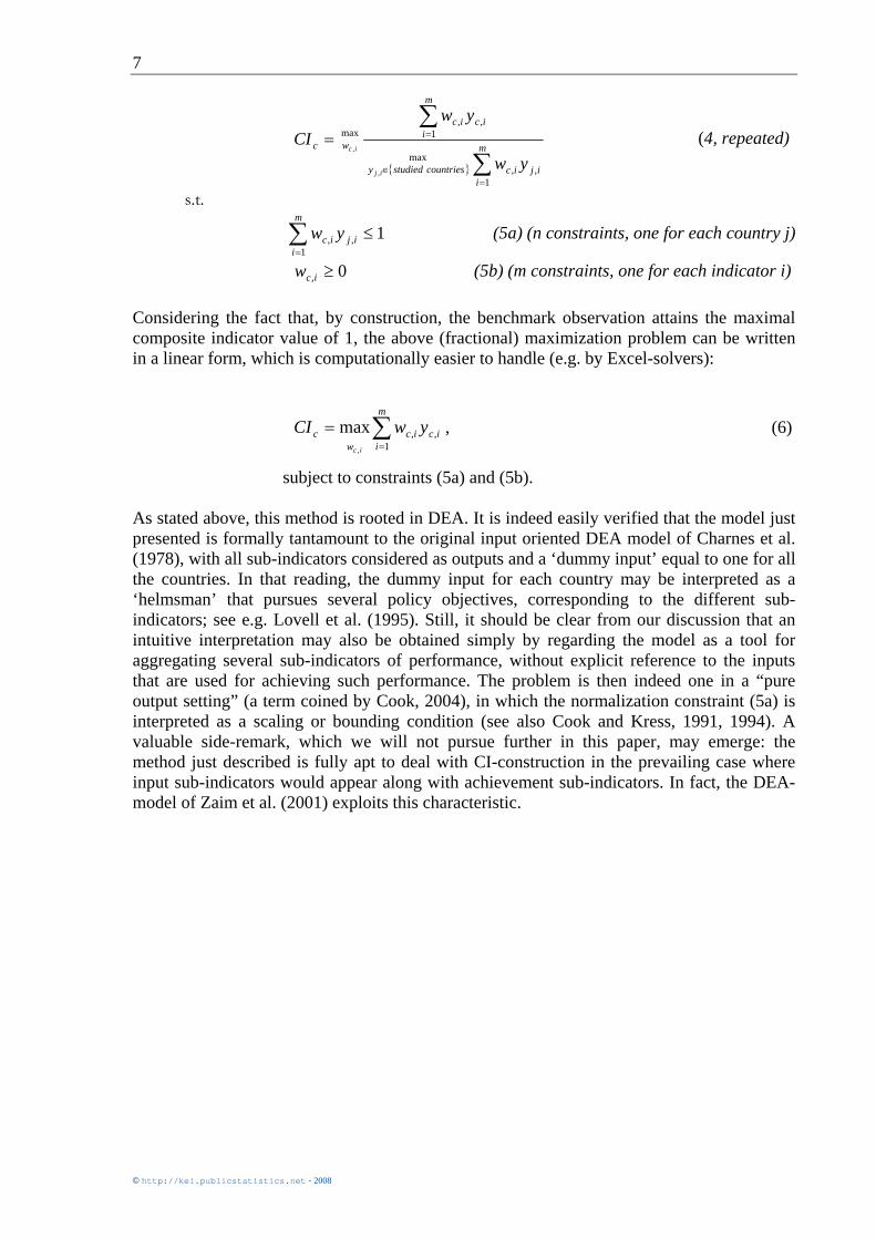
0, ≥icw (5b) (m constraints, one for each indicator i) Considering the fact that, by construction, the benchmark observation attains the maximal composite indicator value of 1, the above (fractional) maximization problem can be written in a linear form, which is computationally easier to handle (e.g. by Excel-solvers):

∑=

=m

iicic

wc ywCI

ic 1,,

,

max , (6)

subject to constraints (5a) and (5b). As stated above, this method is rooted in DEA. It is indeed easily verified that the model just presented is formally tantamount to the original input oriented DEA model of Charnes et al. (1978), with all sub-indicators considered as outputs and a ‘dummy input’ equal to one for all the countries. In that reading, the dummy input for each country may be interpreted as a ‘helmsman’ that pursues several policy objectives, corresponding to the different sub-indicators; see e.g. Lovell et al. (1995). Still, it should be clear from our discussion that an intuitive interpretation may also be obtained simply by regarding the model as a tool for aggregating several sub-indicators of performance, without explicit reference to the inputs that are used for achieving such performance. The problem is then indeed one in a “pure output setting” (a term coined by Cook, 2004), in which the normalization constraint (5a) is interpreted as a scaling or bounding condition (see also Cook and Kress, 1991, 1994). A valuable side-remark, which we will not pursue further in this paper, may emerge: the method just described is fully apt to deal with CI-construction in the prevailing case where input sub-indicators would appear along with achievement sub-indicators. In fact, the DEA-model of Zaim et al. (2001) exploits this characteristic.

8

KEI-WP5-D5.3

Chapter 3 Sub-Indicator Share Restrictions

Apart from the non-negativity of the weights (equation (5b)), the formal model hitherto discussed allows weights to be freely estimated in order to maximize the relative efficiency score of the evaluated country. (The weights are only restricted in that they must not make the final score exceed the upper limit of 1). The advantage of such flexibility is that it becomes hard for countries to argue that the weights themselves put them at a disadvantage. However, there are also disadvantages to this full flexibility. In some situations, it can allow a country to appear as a brilliant performer in a way that is difficult to justify. For example, if some zero weights are assigned, and if there is no prior information which backs up this possibility, some of the achievement indicators do not contribute to a country’s composite measure. One then faces the risk of basing ‘global’ performance on a small subset of all (and often meticulously selected) sub-indicators. Also, by allowing full freedom, resulting outcomes may in particular contradict prior views on weights (e.g. expert opinions). In practice, it is essential for the credibility and acceptance of composite indicators to incorporate the opinion of experts that have a wide spectrum of knowledge, to ensure that a proper weighting scheme is established. True as this may be, it is at the same time also true that, in the area of composite indicator construction, experts may (strongly) disagree about the precise value of the weights. Fortunately, DEA models are able to incorporate such prior information by adding additional restrictions to the basic problem. This seems especially convenient in the common case where experts disagree on weights. In all probability, this is exactly the setting where the benefit of the doubt approach to CIs seems to be most powerful. When individual expert opinion is available, but when experts disagree about the right set of weights, the method is sufficiently flexible to incorporate ‘agreed judgments’ by imposing additional (e.g., sub-indicator share) restrictions. And at the point where disagreement remains, i.e. literarily where no further restrictions can be imposed, the informational gap is filled by choosing country-specific benefit-of-the doubt weights. In our opinion, and with an eye towards practical applications, the latter reasoning may as well be reversed, so as to be more in line with the remark of Foster and Sen cited in section 2.1. That is: it is easier to let experts agree a priori on restrictions than on a unique set of weights. The final result would then reflect what is actually there: limited agreement. Evidently, the nature of such restrictions can vary, and we will now briefly survey some alternatives. Following the unit invariance inherent in DEA, one should be cautious when comparing and interpreting benefit of the doubt weights as they adapt to the units of measurement. Also, if one would impose additional restrictions on the weights (i.e., in addition to (5b)), it may well be difficult to give an instantly recognizable meaning to such restrictions. One escape route is, however, feasible, namely to shift the focus to ‘sub-indicator shares’, which are completely independent of measurement units. Sub-indicator shares are in fact the product of the original value of the sub-indicator icy , and the assigned weight icw ,

4. Referring back to equation (6), the eventual composite indicator can thus be re-interpreted as a sum of i = 1,…,m sub-indicator shares, one for each achievement dimension. Now, these m terms may 4 In the DEA literature, this concept is usually labelled a ‘virtual output’ (‘virtual input’). See especially Thanassoulis, Portella, and Allen (2004) for a discussion of virtual outputs (or pure weights, or exogenous benchmarks) as means to include value judgments in DEA.

9


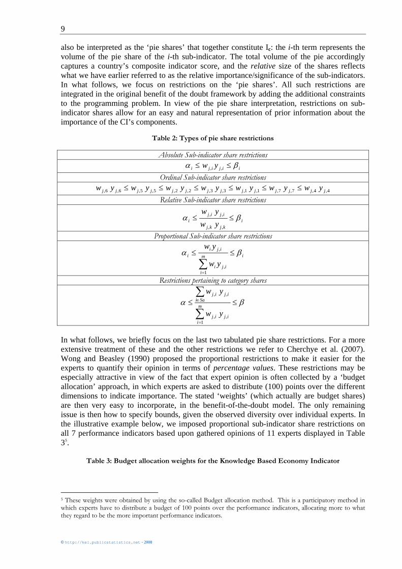
also be interpreted as the ‘pie shares’ that together constitute Ic: the i-th term represents the volume of the pie share of the i-th sub-indicator. The total volume of the pie accordingly captures a country’s composite indicator score, and the relative size of the shares reflects what we have earlier referred to as the relative importance/significance of the sub-indicators. In what follows, we focus on restrictions on the ‘pie shares’. All such restrictions are integrated in the original benefit of the doubt framework by adding the additional constraints to the programming problem. In view of the pie share interpretation, restrictions on sub-indicator shares allow for an easy and natural representation of prior information about the importance of the CI’s components.

Table 2: Types of pie share restrictions

Absolute Sub-indicator share restrictions iijiji yw βα ≤≤ ,,

Ordinal Sub-indicator share restrictions 4,4,7,7,1,1,3,3,2,2,5,5,6,6, jjjjjjjjjjjjjj ywywywywywywyw ≤≤≤≤≤≤

Relative Sub-indicator share restrictions

ikjkj

ijiji yw

ywβα ≤≤

,,

,,

Proportional Sub-indicator share restrictions

im

iiji

ijii

yw

ywβα ≤≤

∑=1

,

,

Restrictions pertaining to category shares

βα ≤≤

∑

∑

=

∈m

iijij

Saiijij

yw

yw

1,,

,,

In what follows, we briefly focus on the last two tabulated pie share restrictions. For a more extensive treatment of these and the other restrictions we refer to Cherchye et al. (2007). Wong and Beasley (1990) proposed the proportional restrictions to make it easier for the experts to quantify their opinion in terms of percentage values. These restrictions may be especially attractive in view of the fact that expert opinion is often collected by a ‘budget allocation’ approach, in which experts are asked to distribute (100) points over the different dimensions to indicate importance. The stated ‘weights’ (which actually are budget shares) are then very easy to incorporate, in the benefit-of-the-doubt model. The only remaining issue is then how to specify bounds, given the observed diversity over individual experts. In the illustrative example below, we imposed proportional sub-indicator share restrictions on all 7 performance indicators based upon gathered opinions of 11 experts displayed in Table 35.

Table 3: Budget allocation weights for the Knowledge Based Economy Indicator

5 These weights were obtained by using the so-called Budget allocation method. This is a participatory method in which experts have to distribute a budget of 100 points over the performance indicators, allocating more to what they regard to be the more important performance indicators.

10

KEI-WP5-D5.3

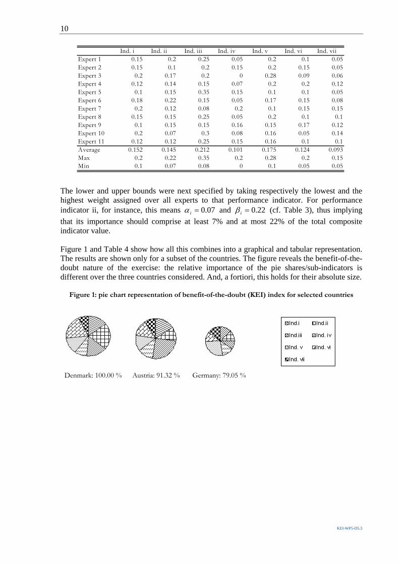
The lower and upper bounds were next specified by taking respectively the lowest and the highest weight assigned over all experts to that performance indicator. For performance indicator ii, for instance, this means 07.0=iα and 22.0=iβ (cf. Table 3), thus implying that its importance should comprise at least 7% and at most 22% of the total composite indicator value. Figure 1 and Table 4 show how all this combines into a graphical and tabular representation. The results are shown only for a subset of the countries. The figure reveals the benefit-of-the-doubt nature of the exercise: the relative importance of the pie shares/sub-indicators is different over the three countries considered. And, a fortiori, this holds for their absolute size.

Figure 1: pie chart representation of benefit-of-the-doubt (KEI) index for selected countries

Denmark: 100.00 % Austria: 91.32 % Germany: 79.05 %

Ind. i Ind. ii Ind. iii Ind. iv Ind. v Ind. vi Ind. vii Expert 1 0.15 0.2 0.25 0.05 0.2 0.1 0.05Expert 2 0.15 0.1 0.2 0.15 0.2 0.15 0.05Expert 3 0.2 0.17 0.2 0 0.28 0.09 0.06Expert 4 0.12 0.14 0.15 0.07 0.2 0.2 0.12Expert 5 0.1 0.15 0.35 0.15 0.1 0.1 0.05Expert 6 0.18 0.22 0.15 0.05 0.17 0.15 0.08Expert 7 0.2 0.12 0.08 0.2 0.1 0.15 0.15Expert 8 0.15 0.15 0.25 0.05 0.2 0.1 0.1Expert 9 0.1 0.15 0.15 0.16 0.15 0.17 0.12Expert 10 0.2 0.07 0.3 0.08 0.16 0.05 0.14Expert 11 0.12 0.12 0.25 0.15 0.16 0.1 0.1Average 0.152 0.145 0.212 0.101 0.175 0.124 0.093Max 0.2 0.22 0.35 0.2 0.28 0.2 0.15Min 0.1 0.07 0.08 0 0.1 0.05 0.05

11


Table 4 6: absolute values and percentage contributions to CI of subindicator shares

Table 4 provides more information. The upper part show the respective countries’ values of sub-indicator shares, which, as indicated, sum up to their composite score. One infers, e.g., that the absolute values of the pie shares of top-ranked Denmark are not always bigger than those corresponding to the other countries that are listed. The underlying ‘revealed evidence’-intuition for these observations is, again, that a country is not likely to put very much weight (and in the limit no weight at all) on dimensions in which it demonstrably has a comparative disadvantage relative to the performance of other countries in the sample. The lower part of the table shows the percentage shares. Percentage contributions further reveal how each country is offered (some) leeway in assigning ‘importance’ to each of the components of the composite index, while at the same time obeying the pie share restrictions stemming from the last two lines of table 4. One notices some similarities, but some huge inter-country differences as well. Often, composite indicators are constructed such that their sub-indicators can be classified in p mutually exclusive categories pSS ,...,1 . Each category then represents a certain orientation or focus of the evaluated phenomenon. Cherchye and Kuosmanen (2004), and Cherchye et al. (2005) show how this can be combined with weight restrictions, and apply this idea to restrictions on “category shares”. Imposing restrictions on these category shares involves a straightforward extension of earlier restrictions. Once more, the idea of imposing restrictions on categories arises from the common observation that it is difficult to define weights for individual sub-indicators. Again the gist of our argument holds: agreement on bounds on the level of categories is much simpler to obtain than specific weights for individual sub-indicators. Indeed, in most cases, focusing on the importance of key categories may allow one to obtain stakeholder consensus more swiftly. Imposing restrictions on categories may be taken as a first step in the quest for consensus among experts.

6 To recall, the 7 sub-indicators are: (Ind. i) Share of ICT sector value added out of total business sector value added (% of total), (Ind. ii) Percentage of individuals using the internet for banking (% of individuals), (Ind. iii) Percentage of firms who use the internet to interact with public authorities (% of firms) , (Ind. iv) Pisa reading literacy of 15 year olds (PISA score points), (Ind. v) Triadic patent families by priority year per million population (number per million population), (Ind. vi) Share of small and medium enterprises (SMEs) collaborating on innovation (% of enterprises), , (Ind. vii) Share of total sales from new-to-firm products (% of total sales).

Ind.i Ind.ii Ind.iii Ind. iv Ind. v Ind. vi Ind. viiCountry ScoreAustria 0.1448 0.1013 0.2329 0.1158 0.1158 0.1158 0.0868 91.32%Germany 0.1009 0.0953 0.0739 0.1053 0.2146 0.0853 0.1153 79.05%Denmark 0.1411 0.2184 0.1514 0.0909 0.1311 0.1911 0.0759 100.00%

Austria 15.86% 11.09% 25.50% 12.68% 12.68% 12.68% 9.50%Germany 12.76% 12.05% 9.35% 13.32% 27.15% 10.79% 14.58%Denmark 14.11% 21.84% 15.14% 9.09% 13.11% 19.11% 7.59%

Sub-indicator shares

Percentage contribution

12

KEI-WP5-D5.3

Chapter 4 Dealing with Imprecise Data

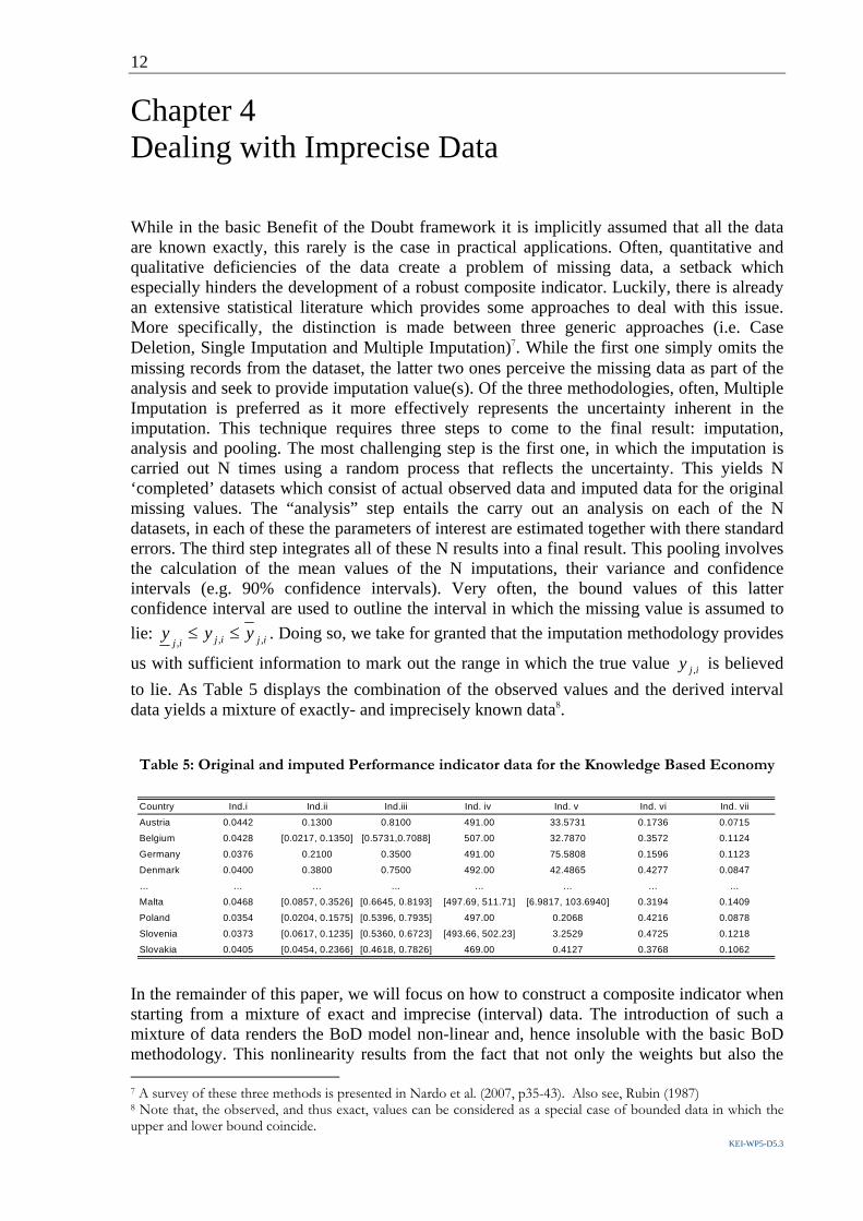
While in the basic Benefit of the Doubt framework it is implicitly assumed that all the data are known exactly, this rarely is the case in practical applications. Often, quantitative and qualitative deficiencies of the data create a problem of missing data, a setback which especially hinders the development of a robust composite indicator. Luckily, there is already an extensive statistical literature which provides some approaches to deal with this issue. More specifically, the distinction is made between three generic approaches (i.e. Case Deletion, Single Imputation and Multiple Imputation)7. While the first one simply omits the missing records from the dataset, the latter two ones perceive the missing data as part of the analysis and seek to provide imputation value(s). Of the three methodologies, often, Multiple Imputation is preferred as it more effectively represents the uncertainty inherent in the imputation. This technique requires three steps to come to the final result: imputation, analysis and pooling. The most challenging step is the first one, in which the imputation is carried out N times using a random process that reflects the uncertainty. This yields N ‘completed’ datasets which consist of actual observed data and imputed data for the original missing values. The “analysis” step entails the carry out an analysis on each of the N datasets, in each of these the parameters of interest are estimated together with there standard errors. The third step integrates all of these N results into a final result. This pooling involves the calculation of the mean values of the N imputations, their variance and confidence intervals (e.g. 90% confidence intervals). Very often, the bound values of this latter confidence interval are used to outline the interval in which the missing value is assumed to lie: ijijij

yyy ,,,≤≤ . Doing so, we take for granted that the imputation methodology provides

us with sufficient information to mark out the range in which the true value ijy , is believed to lie. As Table 5 displays the combination of the observed values and the derived interval data yields a mixture of exactly- and imprecisely known data8.

Table 5: Original and imputed Performance indicator data for the Knowledge Based Economy

In the remainder of this paper, we will focus on how to construct a composite indicator when starting from a mixture of exact and imprecise (interval) data. The introduction of such a mixture of data renders the BoD model non-linear and, hence insoluble with the basic BoD methodology. This nonlinearity results from the fact that not only the weights but also the 7 A survey of these three methods is presented in Nardo et al. (2007, p35-43). Also see, Rubin (1987) 8 Note that, the observed, and thus exact, values can be considered as a special case of bounded data in which the upper and lower bound coincide.

Country Ind.i Ind.ii Ind.iii Ind. iv Ind. v Ind. vi Ind. vii

Austria 0.0442 0.1300 0.8100 491.00 33.5731 0.1736 0.0715

Belgium 0.0428 [0.0217, 0.1350] [0.5731,0.7088] 507.00 32.7870 0.3572 0.1124

Germany 0.0376 0.2100 0.3500 491.00 75.5808 0.1596 0.1123

Denmark 0.0400 0.3800 0.7500 492.00 42.4865 0.4277 0.0847

… … … … … … … …

Malta 0.0468 [0.0857, 0.3526] [0.6645, 0.8193] [497.69, 511.71] [6.9817, 103.6940] 0.3194 0.1409

Poland 0.0354 [0.0204, 0.1575] [0.5396, 0.7935] 497.00 0.2068 0.4216 0.0878

Slovenia 0.0373 [0.0617, 0.1235] [0.5360, 0.6723] [493.66, 502.23] 3.2529 0.4725 0.1218

Slovakia 0.0405 [0.0454, 0.2366] [0.4618, 0.7826] 469.00 0.4127 0.3768 0.1062

13


levels of inputs and outputs are variables to be estimated. The question to be addressed then is how to treat this nonlinearity problem to make BoD applicable. The approach that we will propose is based on a more recent offspring in the DEA literature, namely Imprecise Data Envelopment Analysis (Cooper et al., 1999; Zhu, 2003 and 2004; Despotis et al., 2002 and Park, 2006). Within the context of constructing composite indicators, we will refer to this methodology as Imprecise Benefit of the Doubt (IBoD). Intuitively, when some of the data are imprecise, the constructed composite indicators from this data should be imprecise as well. Therefore, instead of delivering precise values, it makes more sense to compute a range of composite indicator values. The approach of Despotis et al. (2002) and Entani et al. (2002) satisfies this intuition in that it defines an upper and lower bound for the composite indicator value, thereby outlining an interval in which the exact composite indicator is believed to lie. We follow this approach to transform our general BoD approach into an IBoD counterpart to deal with imprecise data. The upper and lower bound composite indicator values hinge upon the distinction between two scenarios9: strong country in weak environment (optimistic scenario) and weak country in strong environment (pessimistic scenario). Both scenarios result from very specific choices of exact data for the evaluated country and the remaining countries in the dataset. In the strong country in weak environment scenario (7a), the evaluated country receives its most favourable imputed performance indicator values ( icy , ), while we select for the other countries their lowest possible ones (

ijy

,). The evaluated country is thus positioned in its

strongest position, while the opposite holds for the other countries. Obviously, this setting yields the evaluated country’s maximum performance indicator value upper

cCI . The reverse happens in the weak country in strong environment case (7b), where the evaluated country is assigned its lowest possible imputed performance indicator values (

icy

,) and the other

countries their highest possible ones ( ijy , ). Unsurprisingly, this scenario results in the

evaluated country’s lower bound composite indicator value lowercCI . In formal mathematical

terms, both scenarios can be presented as follows10:

iWwiw

cjyw

yw

ts

aywCI

ic

ic

ij

m

iic

ic

m

iic

m

iicicwc

ic

∀∈

∀≥

≠∀≤

≤

=

∑

∑

∑

=

=

=

,

,

,1

,

,1

,

1,,

0

1

1

..

)7(max,

iWwiw

cjyw

yw

ts

bywCI

ic

ic

ij

m

iic

ic

m

iic

m

iicicwc

ic

∀∈

∀≥

≠∀≤

≤

=

∑

∑

∑

=

=

=

,

,

,1

,

,1

,

1,,

0

1

1

..

)7(max,

9 The idea to distinguish between both scenarios was originally introduced by Entani et al. (2002). They referred to both scenarios as the ‘optimistic’ and the ‘pessimistic’ scenario. We adjust the labels in line with the setting of country policy performance evaluation. 10 In case of extra weight restrictions, and thus no full flexibility in the weights choice for the countries, one replaces the last constraints in (7a) and (7b) with one or more constraints as in Table 2.

14

KEI-WP5-D5.3

The great similarity with the original BoD should be noted. In fact, the only change occurring is the introduction of the idea to transform the mixture of exact and imprecise data into a data set of exact data11. The resulting composite indicators of both scenarios constitute the interval [ ]upper

clowerc CICI , that covers all possible composite indicator values. The length of the obtained

interval reflects the ambiguity about the real composite indicator value, and it is likely to vary from country to country. Clearly, upper

clowerc CICI ≤ where equality holds in the limiting

case where all underlying performance indicator values are known exactly.

Table 6: Upper and lower bound performance scores for the Knowledge Based Economy

Based on the above mentioned scenarios, Park (2006) introduced a three-group efficiency classification system where the distinction is being made between perfectly efficient, potentially efficient and inefficient entities12. We apply a similar classification system but adjust the labels to our setting of evaluating countries: benchmark countries, potential benchmark countries, and countries open to improvement. The first category is then the set of countries ranked on top (and thus receiving a composite indicator value of 1) in both scenarios. When countries (e.g. Denmark) are outstanding performers irrespective of the scenario we evaluate them in, then there can be little doubt that they are benchmark performers with respect to the others. The second category includes the countries ranked on top in the ‘strong country in weak environment’ scenario but not in the ‘weak country in strong environment’ one (e.g. Austria and Malta). Here, there is still is some doubt on whether they are benchmark or not, as such classification depends on the imputed data that are used for their calculation. The last category consists of countries that are never ranked on top (e.g. Belgium and Germany). Whatever the specific values of the imputed data, such countries always have room for improvement. Park’s intuition behind this classification is thus straightforward and appealing in the context of evaluating countries’ policy performance.

Table 7: Three-group classification of the countries’ Knowledge Based Economy performance

11 Note that in both adjusted models (7a) and (7b) the set of normalization constraints is split in two sets: one set pertaining to the evaluated country, the other set to the other countries. This splitting up is due to the fact that different values are selected for the evaluated country and the other countries. 12 This three-group classification is an extension to Park’s (2004) efficient and inefficient distinction (and thus a two-group classification) and is similar to the { }+++− EEE ,, 12 classification of Despotis et al. (2002).

Country Optimistic Scenario Pessimistic Scenario

Austria 100.00% 85.74%Belgium 83.39% 70.89%Germany 98.04% 71.28%Denmark 100.00% 100.00%… … …Malta 100.00% 84.76%Poland 76.63% 59.48%Slovenia 77.17% 71.12%Slovakia 63.78% 45.31%

15


A combination of both aforementioned approaches (interval composite indicators and the three group classification system) may be advantageous to render the performance scores more swiftly acceptable. Countries are always quite skeptical concerning the use of composite indicators especially when they indicate for them a poor performance relative to the other countries. Within this perspective, the use of such an interval and classification approach may somewhat soften the message and therefore, render it more swiftly acceptable even for poorer performing countries. 13

Chapter 5 Concluding remarks

We recall our starting point for proposing the benefit of the doubt methodology to construct composite indicators: due to insufficiently precise, and probably unverifiable knowledge of the underlying structure of an evaluated composite phenomenon, uncertainty is inherent in the construction of composite indicators. The lack of a standard construction methodology, the disagreement among experts on the importance of the underlying indicators, etc., are just ways in which this uncertainty is manifested. Precisely these methodological aspects have been invoked to undermine the credibility of composite indicators. This defines a clear challenge for those who believe that composite indicators can be a useful tool for communicative purposes, as well as for those who believe that global comparisons of country performance and the closely related idea of benchmarking could eventually promote good policies. Cast against this general background, the preceding pages do certainly not offer a panacea for all problems bound up with composite indicator construction, but some aspects we touched upon may help to prevent getting bogged down in ‘merely’ methodological discussions. The model, the pie share extensions and the model’s adjustment to deal with imprecise data discussed in the previous sections certainly do not exhaust the complete range of conceivable uses of the benefit-of-the-doubt approach. Indeed, we have already hinted at the fact that still other types of weight restrictions are possible. But the tool may be helpful in more general problem settings as well. One such more general setting is, for instance, concerned with dynamic performance evaluation, i.e. one assesses the performance of a group of countries over time. Zaim et al. (2001), and Cherchye et al. (2005) propose a benefit of the doubt 13 For a more elaborate discussion, see Kao (2006, p. 1088).

Country Optimistic Scenario Pessimistic Scenario Evaluation

Austria 100.00% 85.74% Po ten tial Ben chm ark Coun tryBelgium 83.39% 70.89% Coun try Open to Im pro v em en tGermany 98.04% 71.28% Coun try Open to Im pro v em en tDenmark 100.00% 100.00% Ben chm ark Coun try… … … …Malta 100.00% 84.76% Po ten tial Ben chm ark Coun tryPoland 76.63% 59.48% Coun try Open to Im pro v em en tSlovenia 77.17% 71.12% Coun try Open to Im pro v em en tSlovakia 63.78% 45.31% Coun try Open to Im pro v em en t

16

KEI-WP5-D5.3

aggregate performance index closely related to the Malmquist Productivity Index (MPI, first introduced by Malmquist in 1953) to assess countries’ intertemporal performance shifts14. Measuring performance change between two periods essentially boils down to comparing the aggregate sub-indicator performance in both periods. The weights for each of these two periods can again be selected endogenously. An appealing feature of the MPI is that it can be decomposed into a “catching-up”-component and an “environmental change”-component. The catching-up component indicates the performance change that is effectively due to a country’s idiosyncratic improvement: did it get closer to its ‘contemporaneous’ benchmark or not, and by how much? The environmental change component instead focuses on the conduct of benchmarks themselves, measuring the favorable or unfavorable change of best practices between the two periods. Other findings that originate from the vast DEA-literature may be readily applicable to the CI-context as well. For instance, and as we already touched upon, value judgements that originate from stakeholders may also be appended via the introduction of exogenous, possibly ‘hypothetical’ observations, to which all countries could then be compared. Or, to take another example: DEA has been broadened to deal with ordinal variables as well (see Cook, 2004, for a survey), and this clearly is an important extension with an eye towards some existing composite indicators, given that some (partially) build on ‘soft’ (categorical) survey data (e.g., the World Economic Forum’s Competitiveness Index). It is however also important to stress that, today, some possible extensions are best considered as promising avenues for further research. To give an example of the latter as well, recall that in the general DEA framework sub-indicators are linearly aggregated into one single index. An alternative would be the geometric aggregation:

∏=

=m

i

wnicc

icyCI1

,,)( (13)

which, in fact can be ‘linearized’ (by taking logarithms) such that one obtains a model that has a formally similar structure as the basic benefit of the doubt model (4)-(5a)-(5b). However, (i) one needs additional (absolute weight) constraints to preserve unit invariance for this model (see e.g. Cooper, Seiford, Tone, 2000, p. 110-111) which may not always lead to feasible solutions, and (ii) the proper interrelationship of (a logged form of) the geometric aggregation form (13) and expert information on the weights has, to the best of our knowledge, not yet been analyzed. Still, given the current stance of research in this area, the benefit-of-the-doubt approach has some virtues over other, current mainstream approaches to composite indicator construction. As we pointed out, its unit invariance allows us to transcend discussions on the undesirable impact of normalization on eventual country rankings. Its flexible approach to the weighting issue may downplay critical remarks on ‘imputed’ weighting systems. Thirdly, and importantly for practitioners, its fundamental interpretation and the concomitant country results are easy to convey (e.g. by using pie charts), a remark which also holds for the kind of information one seeks to distill from the expert community.

14 Furthermore, similar adjustments could be made to the Imprecise Benefit of the Doubt model.

17


Bibliography Babbie E. (1995): The Practice of Social Research, Wadsworth Publishing Company, Belmont

Booysen F. (2002): “An Overview and Evaluation of Composite Indices of Development”, Social Indicators Research 59, 115-151.

Brandolini A. (2002): “Education and Employment Indicators for the EU Social Agenda”, Politica Economica, Vol. 18, pp. 55-62.

Charnes A., Cooper W. W. and Rhodes E. (1978): “Measuring the Efficiency of Decision Making Units”, European Journal of Operational Research 2, p. 429-444.

Cherchye L, Moesen W. Rogge N., and Van Puyenbroeck T. (2007): “An introduction to ‘benefit of the doubt’ composite indicators”, Social Indicators Research, 82, pp. 111-145.

Cherchye L, Lovell C.A.K., Moesen W. and Van Puyenbroeck T. (2005): “One Market, One number? A Composite Indicator Assessment of EU Internal Market Dynamics”, European Economic Review, Vol 51(3), pp. 749-779.

Cherchye L., Moesen W. and Van Puyenbroeck T. (2004): “Legitimately Diverse, yet Comparable: On Synthesizing Social Inclusion Performance in the EU”, Journal of Common Market Studies, 42, 919-955.

Cherchye L and Kuosmanen T. (2006): “Benchmarking Sustainable Development: A Synthetic Meta-Index Approach” Chapter 7 in M. McGillivray and M. Clarke (eds.), Perspectives on Human Development, United Nations University Press, to appear.

Cook, W.D. (2004), “Qualitative data in DEA”, in W.W. Cooper, L. Seiford, and J. Zhu, Handbook on Data Envelopment Analysis, Kluwer Academic Publishers, 75-97.

Cook, W.D., M. Kress (1991), “A multiple criteria decision model with ordinal preference data”, European Journal of Operations Research 54, 191-193.

Cook, W.D., M. Kress (1994), “A multiple criteria composite index model for quantitative and qualitative data”, European Journal of Operations Research 78, 367-379.

Cooper W.W., Seiford L.M. and Tone K. (2000): Data Envelopment Analysis: A Comprehensive Text with Models, Applications, References and DEA-Solver Software, Kluwer Academic Publishers.

Cooper, W.W., Park, K.S. and Yu, G. (1999): “IDEA and AR-IDEA: Models for Dealing with Imprecise Data in DEA”, Management Science, Vol. 45, No. 4, pp. 597-607.

Desai M., Fukuda-Parr S., Johansson C. and Sagasti F. (2002): “Measuring the Technology Achievement of Nations and the Capacity to Participate in the Networking Age”. Journal of Human Development, Vol. 3, No. 1, 2002.

Despotis, DK (2005), “A reassessment of the human development index via data envelopment analysis”, Journal of the Operational Research Society.

Despotis, D.K. and Smirlis, Y.G. (2002): “Data Envelopment Analysis with Imprecise Data”, European Journal of Operational Research 140, 24-36.

Ebert U. and Welsch H. (2004): “Meaningful Environmental Indices: A Social Choice Approach”, Journal of Environmental Economics and Management, Vol.47, pp. 270-283.

18

KEI-WP5-D5.3

Entani, T., Maeda, Y. and Tanaka, H. (2002): “Dual models of interval DEA and its extensions to interval data”, European Journal of Operational Research 136, 32-45.

European Commission (2004), The EU Economy Review 2004, European Economy, Nr. 6, Office for Official Publications of the EC, Luxembourg.

Foster J. and Sen A. (1997): “On Economic Inequality” (2nd, expanded edn) (Oxford: Clarendon Press)

Freudenberg M. (2003): “Composite Indicators of Country Performance: A Critical Assessment”, OECD Science, Technology and Industry Working Papers 2003/16

Halme, M., Joro, T., Koivu, M. (2002) “Dealing with Interval Scale Data in Data Envelopment Analysis”, European Journal of Operational Research, Vol. 137, 22–27

Hopkins, M. (1991): “Human Development Revisited: A New UNDP Report”, World Development 19, 1469-1473.

Kao, C. (2006): “Interval efficiency measures in data envelopment analysis with imprecise data”, European Journal of Operational Research, 174(2), pp. 1087-1099.

Kao, C. and H.T. Hung (2005), “Data envelopment analysis with common weights: the compromise solution approach”, Journal of the Operational Research Society, 56, 1196-1203.

Kumar S. and Russel R.R. (2002): “Technical Change, Technological Catch-Up, and Capital Deepening: Relative Contributions to Growth and Convergence”, American Economic Review 92, 527-548.

Lovell C.A.K, Pastor J.T. and Turner J.A. (1995): “Measuring Macroeconomic Performance in the OECD: A Comparison of European and Non-European Countries”, European Journal of Operational Research, 87 (1995), 507-518.

Mahlberg B. and Obersteiner M. (2001): “Remeasuring the HDI by Data Envelopment Analysis”, International Institute for Applied Systems Analysis Interim Report 01-069.

Melyn W. and Moesen W. (1991): “Towards a Synthetic Indicator of Macroeconomic Performance: Unequal Weighting when Limited Information is Available, Public Economics Research Paper 17, CES, KU Leuven.

Micklewright J. (2001): “Should the UK Government Measure Poverty and Social Exclusion with a Composite Index?” in CASE, Indicators of progress: A Discussion of Approaches to Monitor the Government’s Strategy to Tackle Poverty and Social Exlusion, CASE Report 13, London School of Economics.

Munda G. and Nardo M. (2003): “On the Methodological Foundations of Composite Indicators Used for Ranking Countries”, mimeo, Universitat Autonoma de Barcelona.

Nardo M., Saisana M., Saltelli A. and Tarantola S. (EC/JRC) and Hoffman A and Giovannini E. (OECD) (2005): Handbook on Constructing Composite Indicators: Methodology and User Guide, OECD Statistics Working Paper

Nardo, M., Saisana, M., Saltelli, A. and Tarantola, S. (2007): Input to Handbook of Good Practices for Composite Indicator’s Development, KEI-project: Workpackage 5, Deliverable 5.2., p35-43.

Park, K.S. (2006): “Efficiency bounds and efficiency classifications in DEA with imprecise data”, Journal of the Operational Research Society, pp.1-8.

19


Park, K.S. (2004): “Simplification of the transformations and redundancy of assurance regions in IDEA (imprecise DEA)”, Journal of the Operational Research Society, 55, 1363-1366.

Pedraja-Chaparro F., Salinas-Jimenez J. and Smith P. (1997): “On the Role of Weight Restrictions in Data Envelopment Analysis”, Journal of Productivity Analysis 8, 215-230.

Roll Y., Cook W.D. and Golany B. (1991): “Controlling Factor Weights in Data Envelopment Analysis”, IIE Transactions 23/1, 2-9.

Rubin, D.B. (1987): Multiple Imputation for Nonresponse in Surveys, Wiley, New York.

Saisana, M., A. Saltelli, and S. Tarantola (2005), “Uncertainty and Sensitivity Analysis as tools for the quality assessment of composite indicators”, Journal of the Royal Statistical Society Series A, 168, 1-17.

Semple, J. (1996), “Constrained games for evaluating organizational performance”, European Journal of Operational Research, 96, 103-112.

Storrie D. and Bjurek H. (2000): “Benchmarking European Labour Market Performance with Efficiency Frontier Techniques”, CELMS Discussion Paper, Göteborg University.

Thanassoulis E., Portela M.C. and Allen R. (2004): “”Incorporating Value Judgements in DEA”, in W.W. Cooper, L. Seiford, and J. Zhu, Handbook on Data Envelopment Analysis, Kluwer Academic Publishers, p. 99-138.

Wong Y.H.B. and Beasly J.E. (1990): “Restricting Weight Flexibility in Data Envelopment Analysis”, Journal of the Operational Research Society 41, 829-835.

Zaim, O., Färe, R., and Grosskopf, S. (2001), “An Economic Approach to Achievement and Improvement Indexes”, Social Indicators Research 56, 91-118.

Zhu, J. (2004): “Imprecise DEA via standard linear DEA models with a revisit to a Korean mobile telecommunication company”, Operations Research, 52, pp. 323-329.

Zhu, J. (2003): “Imprecise Data Envelopment Analysis (IDEA): A review and improvement with an application”, European Journal of Operational Research 144, pp. 513-529.

Zhu, J. (2003), Quantitative Models for Performance Evaluation and Benchmarking, International series in operations research and management science, Kluwer Academic Publishers.

workpackage 5 ‘benefit of the doubt’ composite indicators

Documents