WORKPLACE HETEROGENEITY AND THE RISEOF WEST GERMANWAGE INEQUALITY∗

David CardDepartment of Economics, UC Berkeley

Jörg HeiningInstitute for Employment Research (IAB), Germany

Patrick KlineDepartment of Economics, UC Berkeley

Abstract

We study the role of establishment-specific wage premiums in generating recentincreases in West German wage inequality. Models with additive fixed effects for work-ers and establishments are fit in four sub-intervals spanning the period from 1985 to2009. We show that these models provide a good approximation to the wage struc-ture and can explain nearly all of the dramatic rise in West German wage inequality.Our estimates suggest that the increasing dispersion of West German wages has arisenfrom a combination of rising heterogeneity between workers, rising dispersion in thewage premiums at different establishments, and increasing assortativeness in the as-signment of workers to plants. In contrast, the idiosyncratic job-match component ofwage variation is small and stable over time. Decomposing changes in mean wagesbetween different education groups, occupations, and industries, we find that increas-ing plant-level heterogeneity and rising assortativeness in the assignment of workers toestablishments explain a large share of the rise in inequality along all three dimensions.JEL Codes: J00, J31, J40

∗Corresponding author: Patrick Kline, 530 Evans Hall #3880, Berkeley, CA 94720; email:pkline@econ.berkeley.edu. We thank the Berkeley Center for Equitable Growth for funding support. We aregrateful to the IAB and to Stefan Bender for assistance in making this project possible, and to Karl Schmidt,Robert Jentsch, Cerstin Erler, and Ali Athmani for invaluable assistance in running our programs at theIAB. We also thank Christian Dustmann, Bernd Fitzenberger, and seminar participants at EUI Florence,Yale, Stanford, and the NBER Labor Studies meetings for many helpful comments and suggestions. RobertHeimbach, Hedvig Horvath, and Michele Weynandt provided excellent research assistance.

1

I Introduction

Wage inequality has risen in many countries, attracting the sustained attention of policy

makers and the general public (see Katz and Autor [1999]; and Acemoglu and Autor [2011]

for detailed reviews). Most existing studies explain the rise in inequality as a consequence

of supply and demand factors that have expanded the productivity gap between high- and

low-skilled workers (e.g., Katz and Murphy [1992], Bound and Johnson [1992], Juhn, Murphy

and Pierce [1993], Goldin and Katz [2008]). Economists have long recognized, however, that

some firms pay higher wages than others for equally skilled workers (e.g., Slichter [1950],

Rees and Schultz [1970], Krueger and Summers [1988], Van Reenen [1996]). The magnitude

of this workplace component of wage inequality is explored in several recent papers, includ-

ing Abowd, Kramarz, and Margolis [1999], Goux and Maurin [1999], Abowd, Creecy, and

Kramarz [2002], Gruetter and Lalive [2009] and Holzer et al. [2011].1 Virtually all these

studies find significant employer-specific wage differentials. To date, however, there is little

evidence on whether these differentials have widened over time, and if so whether they can

help explain the rise in cross-sectional wage inequality.2

In this paper we use detailed administrative data from West Germany to study trends

in the dispersion of the workplace-specific wage premiums earned by individuals on different

jobs, and measure the contribution of workplace heterogeneity to the rise in inequality. Wage

inequality has widened substantially in Germany over the past two decades (see Dustmann,

Ludsteck, and Schönberg [2009]). Figure I, for example, shows the evolution of various real

wage percentiles for full time male workers in West Germany, indexed to a base of 1996.3

Over the 13-year period from 1996 to 2009, the gap between the 20th and 80th percentiles of

1An earlier generation of studies (e.g., Davis and Haltiwanger [1991], Groshen [1991], Bernard and Jensen[1995]) documented substantial between-plant variation in wages but was unable to deal fully with nonrandomassignment of workers to firms.

2Barth et al. [2011] find that between plant inequality has grown over time in the U.S. but are unableto fully account for changes in the pattern of sorting of workers to firms due to limitations in their data.Cardoso [1997, 1999] provides evidence that between plant wage variation grew in Portugal but is againunable to fully account for selection of workers into firms based upon unobservables. Skans et al. [2009]provide similar between-plant evidence for Sweden.

3The data underlying this figure are described in detail in Section III, below.

2

wages expanded by approximately 20 log points, roughly comparable to the rise in inequality

in the U.S. labor market over the 1980s.4

The German labor market presents an important test case for assessing changes in wage-

setting behavior and the role of firm-specific heterogeneity. After a decade or more of disap-

pointing economic performance (Siebert [1997]), the country implemented a series of labor

market reforms in the late 1990s and early 2000s, and has recently emerged as one of the

most successful economies in the OECD.5 There is widespread interest in the sources of this

recent success and the lessons it may hold for other countries.

To separately identify the impact of rising heterogeneity in pay across different workers

and rising heterogeneity in the pay received by the same individual on different jobs, we

divide the period between 1985 and 2009 into four overlapping intervals and fit separate

linear models in each interval with additive person and establishment fixed effects, as in

Abowd, Kramarz, and Margolis [1999] —henceforth, AKM. We then compare the estimates

of the person and establishment effects across intervals to decompose changes in the structure

of wages.

In an initial methodological contribution we present new evidence on the quality of the

approximation to the wage structure provided by AKM’s additive worker and firm effects

specification. We show that the strong separability assumptions of the AKM model are

nearly (but not perfectly) met in the data. In particular, generalized non-separable models

with fixed effects for each job yield only a small improvement in explanatory power relative

to the AKM specification, both within narrow time intervals and between intervals. We also

check for patterns of endogenous mobility that could lead to systematic biases in the AKM

specification and find little evidence of such patterns.

Our main substantive contribution is a simple decomposition of the rise in wage inequality

4For example, Katz and Murphy [1992] show that the 90-10 gap in log weekly wages for full time maleworkers rose by 0.18 between 1979 and 1987, while Autor, Katz and Kearney [2008] show that the 90-10 gapin log weekly wages for full time full year male workers rose by 0.25 between 1979 and 1992.

5For overviews of recent changes in the German labor market see Eichhorst and Marx [2009], Burda andHunt [2011], and Eichhorst [2012].

3

among full time male workers in West Germany. We find that the increase is attributable

to increases in the dispersion of both the person-specific and workplace-specific components

of pay, coupled with a rise in the assortativeness of job matching that magnifies their joint

effect.6 Overall, the rise in the variance of the person component of pay contributes about

40% of the overall rise in the variance of wages, the rise in the establishment component

contributes around 25%, and their rising covariance contributes about a third. We find

qualitatively similar results for full time female workers.

We go on to use our estimated models to decompose the rise in between-group inequality

across different education, occupation, and industry groups. We find that two-thirds of

the increase in the pay gap between higher and lower-educated workers is attributable to

a widening in the average workplace pay premiums received by different education groups.

Increasing workplace heterogeneity and rising assortativeness between high-wage workers and

high-wage firms likewise explain over 60% of the growth in inequality across occupations and

industries.

Finally, we investigate two potential channels for the rise in workplace-specific wage

premiums: establishment age and collective bargaining status. Classifying establishments

by entry year, we find a trend toward increasing heterogeneity among establishments that

entered the labor market after the mid-1990s, coupled with relatively small changes in the

dispersion of the premiums paid by continuing establishments. The relative inequality among

newer establishments is linked to their collective bargaining status: an increasing share of

these establishments have opted out of the traditional sectoral contracting system and pay

relatively low wages. These patterns suggest that rising wage inequality in West Germany

is related to institutional changes in the wage setting process, though the underlying source

of these coincident trends is less clear.6Recent contributions by Andersson et al. [2012] and Bagger, Sorensen, and Vejlin [2012] also document

increases in assortative matching between workers and employers. Those studies use related statisticalmethods but assume that person and establishment effects are stationary over the entire sample period.

4

II Background - Macro Trends and Institutional Changes

As background for our empirical analysis this section briefly summarizes some of the major

changes that have affected the West German labor market since the early 1980s. Two

critical events were the collapse of the Soviet empire and the reunification of East and

West Germany.7 An immediate consequence of these political developments was massive in-

migration to West Germany. Approximately 1.7 million former residents of East Germany

moved to the west in the early 1990s (see Burda [1993] and Wolff [2009]). An even larger

number of ethnic Germans (approximately 2.8 million people) arrived from Russia and the

former East Bloc countries during the 1990s (Bauer and Zimmerman [1999]). These new

migrants —many of whom lacked modern training and language skills —contributed to the

rise in unemployment in West Germany (Glitz [2012]) and the build-up of pressure for labor

market reform.

More subtly, the decision to impose West German wage scales on the less-productive

East led to fissures in the traditional collective bargaining system (Burda [2000]). Until the

1990s most West German firms accepted the provisions of the major sectoral agreements

negotiated between employer associations and large unions. These pay scales proved to be

far too high for East German firms, however, leading to massive defections from the system

—a process that is allowable under German law (see Ochel [2003]). Eventually the defections

spilled over to the West, prompting a sharp decline in the fraction of employees covered

by collective agreements. For example, data presented by Kohaut and Ellguth [2008] and

Ellguth, Gerner, and Stegmaier [2012] show a fall in collective bargaining coverage in West

Germany from 83% in 1995 to 63% in 2007.8

A second and related phenomenon is the adoption of “opt-out”or “opening”clauses by

7These processes began in the late 1980s and ended in the early 1990s. The Berlin wall fell in November1989. Economic reunification was achieved in spring 1990 with the elimination of the East German mark inJune of that year. The country was offi cially reunified in October 1990.

8As discussed by Fitzenberger et al. [2012], not all workers in a given establishment necessarily have thesame contractual coverage status. For example, managers and temporary workers (who are included in ourdata set) are exempt. The coverage rates in the text assign a single establishment status to all employeesand should be interpreted carefully.

5

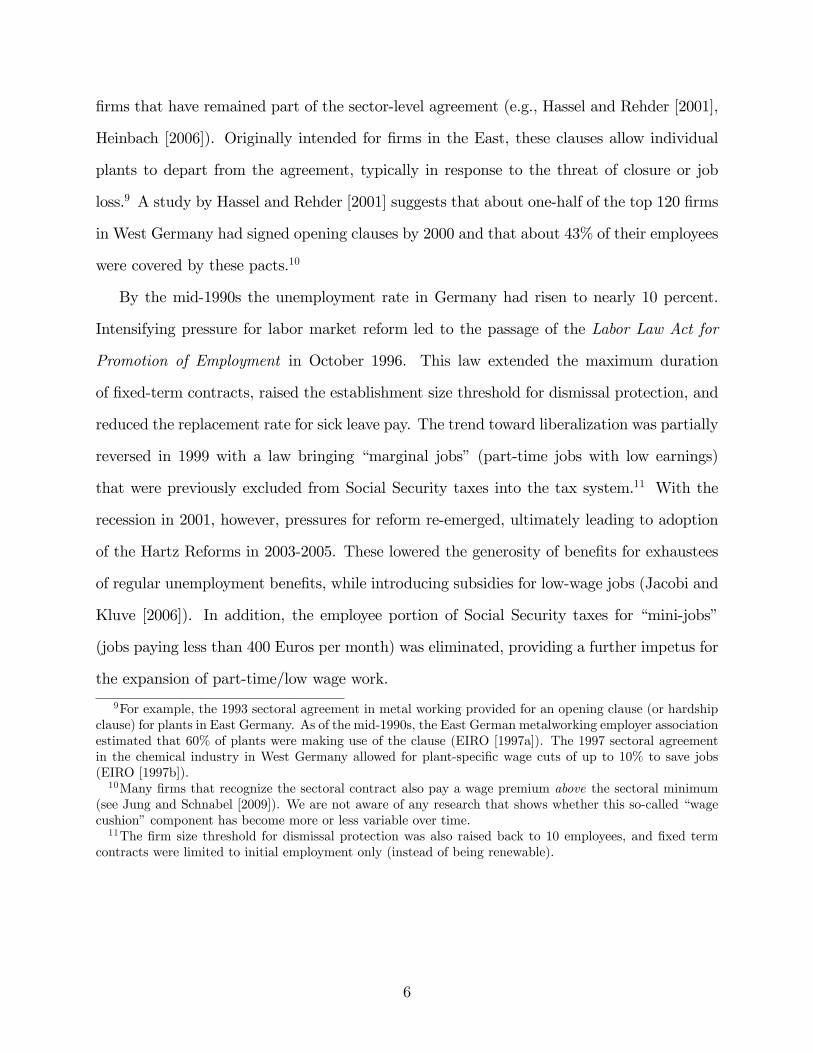
firms that have remained part of the sector-level agreement (e.g., Hassel and Rehder [2001],

Heinbach [2006]). Originally intended for firms in the East, these clauses allow individual

plants to depart from the agreement, typically in response to the threat of closure or job

loss.9 A study by Hassel and Rehder [2001] suggests that about one-half of the top 120 firms

in West Germany had signed opening clauses by 2000 and that about 43% of their employees

were covered by these pacts.10

By the mid-1990s the unemployment rate in Germany had risen to nearly 10 percent.

Intensifying pressure for labor market reform led to the passage of the Labor Law Act for

Promotion of Employment in October 1996. This law extended the maximum duration

of fixed-term contracts, raised the establishment size threshold for dismissal protection, and

reduced the replacement rate for sick leave pay. The trend toward liberalization was partially

reversed in 1999 with a law bringing “marginal jobs” (part-time jobs with low earnings)

that were previously excluded from Social Security taxes into the tax system.11 With the

recession in 2001, however, pressures for reform re-emerged, ultimately leading to adoption

of the Hartz Reforms in 2003-2005. These lowered the generosity of benefits for exhaustees

of regular unemployment benefits, while introducing subsidies for low-wage jobs (Jacobi and

Kluve [2006]). In addition, the employee portion of Social Security taxes for “mini-jobs”

(jobs paying less than 400 Euros per month) was eliminated, providing a further impetus for

the expansion of part-time/low wage work.

9For example, the 1993 sectoral agreement in metal working provided for an opening clause (or hardshipclause) for plants in East Germany. As of the mid-1990s, the East German metalworking employer associationestimated that 60% of plants were making use of the clause (EIRO [1997a]). The 1997 sectoral agreementin the chemical industry in West Germany allowed for plant-specific wage cuts of up to 10% to save jobs(EIRO [1997b]).10Many firms that recognize the sectoral contract also pay a wage premium above the sectoral minimum

(see Jung and Schnabel [2009]). We are not aware of any research that shows whether this so-called “wagecushion”component has become more or less variable over time.11The firm size threshold for dismissal protection was also raised back to 10 employees, and fixed term

contracts were limited to initial employment only (instead of being renewable).

6

III Data

We use earnings records from the German Social Security system that have been assembled

by the Institute for Employment Research into the Integrated Employment Biographies

(IEB) datafile (see Oberschachtsiek et al. [2009]). These data include total earnings and

days worked at each job in a year, as well as information on education, occupation, industry

and part-time or full time status. With the exception of civil servants and self-employed

workers, nearly all private sector employees in Germany are currently included in the IEB.

For our main analysis we focus on daily wages at full-time jobs held by men age 20-60.

Since the IEB does not include hours of work, limiting attention to full time jobs reduces the

impact of hours dispersion that could confound trends in inequality.12 Fewer than 7 percent

of male workers in the IEB have no full time job in a year, so the inclusion of wages for

part-time men has only a small impact on the trends we study. As a check on our main

conclusions we present a parallel analysis for full-time female workers. A smaller majority

of German women work full time (e.g., only about 64% in 2000), raising potential concerns

about selectivity biases.13 Unfortunately, many part-time women work in mini-jobs that

were not covered by Social Security until 1999, so it is diffi cult to study trends for part-time

female workers using IEB data. The available data, however, suggest that general trends for

all female workers are not be too different from those for full time women (see below).

To construct our sample we begin with the universe of full time jobs held by workers

age 20-60 in each year from 1985 to 2009. We exclude mini-jobs (which are only included

after 1999) and jobs in which the employee is undergoing training. As explained in more

detail in the Online Appendix, we sum the earnings received by a given individual from each

12A detailed analysis by Dustmann, Ludsteck, and Schönberg [2009, Appendix Table 7] of data from theGerman Socio-economic Panel shows no change in the variance of hours among full time male workers inWest Germany after 1990, suggesting that hours variation is not a major source of the rise in wage dispersionwe document.13The relative size of the full time female workforce has been relatively stable over the past 25 years,

suggesting that the selectivity biases among full time workers may be relatively constant. The rise in femaleemployment rates since the mid-1990s in Germany has mainly occurred through an expansion of part-timeemployment.

7

establishment in each year and designate the one that paid the highest total amount as the

main job for that year. Most full time workers are employed at only one establishment in

any year (the average is around 1.1 per year) and there is no trend in the number of jobs

held per year, so we believe the restriction to one job per year is innocuous (see Appendix

Table A.1). We calculate the average daily wage by dividing total earnings by the duration

of the job spell (including weekends and holidays). An individual who has no full time job

in a given calendar year is assigned a missing wage for that year.

The establishment identifiers in the IEB are assigned for administrative purposes and

may combine multiple work sites owned by the same firm if they are in the same industry

and municipality. A new establishment identifier (EID) is issued whenever a plant changes

ownership, so the “death”of an establishment identifier does not necessarily mean that the

plant has closed, nor does the “birth”of a new EID necessarily mean that a new plant has

opened.14 While this makes it diffi cult to identify plant closings, for purposes of modeling

wage determination we believe it is appropriate to treat an ownership change as a potential

change in the workplace component of pay, even when a plant remains open. A new owner,

for example, may introduce a bonus system that alters the workplace component of pay. In

cases where a new EID is assigned to a continuing plant, there is no bias in treating the

“new”EID as a new establishment, only a potential loss in effi ciency, since the old and new

establishments can have the same impacts on wages.

Table I illustrates some basic characteristics of our wage data, showing information for

every 5th year of the sample for men in the upper panel and women in the lower panel. The

data set includes 12 to 14 million full time male wage observations in any year, and 6 to 7

million full time female wage observations. As shown in column 2 of the table, average real

daily wages of full time men rose by about 8% between 1985 and 1990, then were relatively

stable over the next 20 years. Average real daily wages of full time women rose by 11%

between 1985 and 1990 and another 6% between 1990 and 1995, but then stabilized at a

14Using clusters of worker flows between establishments, Schmeider and Hethey [2010] estimate that onlyabout one half of EID births and deaths in the IEB are true plant openings or closings.

8

level about 30 log points below the mean for men.15 The standard deviation of log wages for

both gender groups rose slightly between 1985 and 1995, then surged over the next 15 years,

rising by 12 log points for men and 10 log points for women from 1995 to 2009.

An important limitation of the IEB data is the censoring of earnings at the Social Security

maximum. As shown in column 4 of Table II, 10 to 12 percent of male wage observations

and 1 to 3 percent of female wage observations are censored in each year. To address the

problem of censoring we follow Dustmann, Ludsteck, and Schönberg [2009] and use a series of

Tobit models —fit separately by gender, year, education level (5 categories), and age range (4

10-year ranges) —to stochastically impute the upper tail of the wage distribution. Since our

primary interest is in models that include person and establishment effects, we develop an

imputation procedure that captures the patterns of within person and within establishment

dependence in the data. Specifically, our Tobit models for a given year include the worker’s

earnings and censoring rate in all other years, as well as the mean earnings and censoring rate

of his or her co-workers in that year. Using the estimated parameters from these models, we

replace each censored wage value with a random draw from the upper tail of the appropriate

conditional wage distribution (see the Online Appendix for details).

The impact of this imputation procedure is illustrated in columns 5 and 6 of Table I,

where we show the means and standard deviations of log daily wages after replacing censored

observations with allocated values from the Tobit models. For women the means and stan-

dard deviations are only slightly higher than in columns 2 and 3, reflecting the relatively low

censoring rates. For men, the allocation procedure matters more: on average the imputation

raises the estimated mean log wage by 2.7 percentage points and the estimated standard de-

viation by 4.5 percentage points, with slightly larger effects in years with a higher censoring

rate.

Although we believe that this imputation procedure works reasonably well, a natural

concern is that our results —particularly for men —would be somewhat different if we used

15See Anotnczyk, Fitzenberger, and Sommerfeld [2010] for further discussion of recent trends in male-female wages differences in Germany.

9

a different technique.16 To address this concern, we present robustness checks based on the

subset of full time male workers with apprenticeship training. This group, which includes

about 60 percent of the German male workforce, has relatively low censoring rates. As

we show below, our main conclusions are very similar when we use only the apprentice

subsample.

IV Overview of Trends in Wage Inequality

Figure II plots four measures of wage dispersion for full time males: the standard deviation of

log wages (including imputed wages for censored observations), the gap in log wages between

the 80th and 20th percentiles, the gap between the 80th and 50th percentiles, and the gap

between the 50th and 20th percentiles. To facilitate comparisons we normalize the gap

measures by dividing by the corresponding percentile gaps of a standard normal variate.17 If

log wages were normally distributed, the normalized gaps and the standard deviation would

all be equal. While this is evidently not the case, the trends in the standard deviation and

the normalized gaps are quite similar. In particular, the standard deviation rose by 15 log

points from 1985 to 2009, the (normalized) 80-20 gap rose by 16 log points, the 80-50 gap

rose by 15 log points, and the 50-20 gap rose by 18 log points. Since the gap measures are

unaffected by censoring, these similarities suggests that our imputation procedure does not

lead to major biases in estimating the change in wage dispersion over time. Another notable

feature of the data in Figure II is that the growth rates in all four measures of inequality

increased in the mid-1990s. For example, the growth rate of the standard deviation of log16Dustmann, Ludsteck, and Schönberg [2009] present an extensive robustness analysis in which they

evaluate several alternatives to their basic Tobit imputation models, and conclude that they give similarresults. We conducted our own validation exercise by taking data for younger men with apprenticeshiptraining (who have censoring rates under 1%), artificially censoring the data at thresholds such that 10, 20,30, or 40 percent of the observations were censored, applying the same Tobit models used in our main analysisto these samples, imputing the upper tail observations in each sample, and then re-estimating trends in thedispersion of wages. The results, summarized in the online Appendix, suggest that use of imputed wagesleads to a slight upward bias in the measured variance of wages in each year, but no bias in the measuredtrend in inequality.17For example, we divide the 80-20 gap by Φ−1(0.8)−Φ−1(0.2) = 1.683, where Φ (.) represents the standard

normal distribution function.

10

wages increased from 0.23 log points per year in the 1985-1996 period to 0.96 log points per

year from 1996 to 2009.

Figure III compares the trend in the normalized 80-20 wage gap for full time men with

the trends for three other groups of workers: all men (i.e., full- and part-time), full time

women, and all women.18 As noted earlier, the fraction of male workers with no full-time

job in a year is relatively low in West Germany (around 2% in 1985, and just under 7%

in 2008), so the addition of part-time workers to the male sample has only a small effect

on measured inequality. Wage inequality among full time female workers is higher than

among full time men and rises a little less over our sample period, though the general trends

for the two groups are quite similar. Inequality in daily wages for all regularly employed

females (i.e., including all jobs except untaxed mini-jobs) is even higher, perhaps reflecting

the variation in hours of work among part-timers, but rises more slowly than for full time

women or men. Even for the broadest sample of female workers, however, there is evidence

of an acceleration in inequality in the mid-1990s. Given the broad similarity in trends across

the various groups, we concentrate for the remainder of this section on full time men. We

return to consider full time women in more detail in Section VI.

Trends in Residual Wage Inequality

Starting with the seminal U.S. studies by Katz and Murphy [1992] and Bound and Johnson

[1992], analysts have noted that a large share of recent rises in wage inequality have occurred

within conventional skill groups. This is also true in West Germany, as we show in Figure IV,

which plots the residual standard deviations of log wages from a series of linear regression

models, each fit separately by year. As a point of departure the top line in the figure shows the

trend in the unadjusted standard deviation of wages, which rises from 0.37 to 0.52 between18For this analysis we use the Sample of Integrated Labor Market Biographies (SIAB), a two-percent

public use sample that combines information from the IEB with other administrative data bases (Dorneret al. [2011]). We use the same procedures as for our IEB sample but do not impute wages for censoredobservations. Riphahn and Schnitzlein [2011] use the SIAB data to document trends in inequality for menand women together in West and East Germany. Their results for West Germany are very similar to ours.They show that wage inequality in East Germany has risen somewhat faster than in the West.

11

1985 and 2009. The second line in the figure is the standard deviation of the residuals from

a standard Mincerian earnings function (with dummies for four education levels and a cubic

experience term) fit separately by year. Residual inequality rises a little less than overall

wage inequality (from 0.30 in 1985 to 0.43 in 2009), but exhibits the same shift in trend in

the mid-1990s.

Several recent studies have suggested that part of the rise in U.S. wage inequality is

attributable to a rise in the variation in wages across industries (e.g., Bernard and Jensen

[1995]) and/or occupations (e.g., Autor, Levy and Murnane [2003]; Autor, Katz and Kearney

[2008]). The third, fourth and fifth lines in the figure show the trends in the residual standard

deviation of wages after controlling for industry (∼300 dummies with separate coeffi cients

in each year), occupation (∼340 dummies), and industry × occupation (∼28,000 dummies).

While time-varying industry and occupation controls clearly add to the explanatory power

of a standard wage equation, they have only a modest impact on the trend in residual

inequality.19 We return in Section VI, below, to examine trends in between-occupation and

between-industry inequality in light of our econometric decomposition of wage inequality

into person and establishment effects.

In contrast to the rather modest effect of industry and occupation controls, the bottom

line in Figure IV shows that adding dummies for each establishment (with year-specific

coeffi cients) has a sizeable impact on the trend in inequality. Within-plant inequality, as

measured by the residual standard error of the regression model rises by only 0.05 between

1985 and 2009, compared to the 0.13 rise for the baseline model that controls for education

and experience. This contrast suggests that rising heterogeneity in wages offered by different

employers may explain some of the rise in German wage inequality. We caution, however, that

non-random sorting of workers to establishments makes it very hard to interpret the estimates

19A basic human capital model (dummies for education and cubic in experience) has an R2 coeffi cient ofabout 0.35. Adding industry or occupation controls raises the R2 to about 0.50. Adding the interaction ofoccupation and industry raises it to about 0.60. In an earlier draft (Card, Heining and Kline [2012]) we alsopresented specifications that control for Federal State. However, there is little change in mean wages acrossstates so these controls add very little to the basic Mincer specification.

12

from wages models with establishment effects but no controls for unobserved worker skills.

Even if there are no workplace-specific wage premiums, one could still observe significant

and increasingly important establishment effects if workers at the same establishment have

similar unobserved abilities and the returns to these abilities are rising over time, or if the

degree of sorting across establishments is rising.

To study trends in workplace sorting we developed two indexes that are described at

greater length in an earlier version of this paper (Card, Heining and Kline [2012]). The first

is an index of educational sorting based on the coeffi cient from a regression of the mean level

of schooling at worker i′s establishment in year t on his own schooling measured in that year.

As noted by Kremer and Maskin [1996], this coeffi cient can range from 0 (no sorting) to 1

(perfect sorting). The value of the index for full time male workers increases steadily, from

0.34 in 1985 to 0.47 in 2009.

Our second measure of sorting examines the degree of occupational segregation across

workplaces. Specifically, we divide three digit occupations into 10 equally sized groups, based

on mean wages in each occupation during the period 1985-1991. We then compute Theil

indices of segregation for the decile groups across establishments in each year. The Theil

index ranges from 0 (perfect integration) to 1 (perfect segregation) and can be interpreted as

a rescaled likelihood ratio test for the null hypothesis that every establishment employs the

national occupation mix (Theil and Finezza [1971]). Over our sample period the index rises

steadily from 0.46 to 0.53, implying that high- and low-wage occupations are increasingly

segregated between establishments.

Overall we conclude that the degree of sorting of different education and occupation

groups to different establishments has risen in West Germany over our sample period. This

rise may account for some share of the the increasing importance of establishment effects in

a wage model.

13

An Event Study Analysis of the Effect of Job Changes on Wages

If the variation in wages across establishments is mainly due to sorting then people who

change workplaces will not necessarily experience systematic wage changes. If, on the other

hand, different establishments pay different average wage premiums, then individuals who

join a workplace where other workers are highly paid will on average experience a wage gain,

while those who join a workplace where others are poorly paid will experience a wage loss.

Figures Va and Vb present simple event-study analyses that examine the wage effects of job

transitions in the early (1985-1991) and later (2002-2009) years of our sample, classifying the

origin and destination workplaces by the mean wages of other workers at those workplaces.

Specifically, we begin by calculating the distribution of mean co-worker wages across all

person-year observations in a given time interval (1985-91 or 2002-09). For job changers with

at least two consecutive years in both the old and new jobs, we classify the old job based

on the quartile of co-worker mean wages in the last year at that job, and the new job based

on the quartile of co-worker mean wages in the first year on that job. We then assign job

changers to 16 cells based on the quartiles of co-worker wages at the origin and destination

workplaces. Finally, we calculate mean wages in the years before and after the job change

event in each cell.20

For clarity the figures only show the wage profiles for workers leaving quartile 1 and quar-

tile 4 jobs (i.e., those with the lowest-paid and highest-paid co-workers). Online Appendix

Table A.3 provides a complete listing of mean wages before and after the job change event

for each of the 16 cells in the two intervals. In that table we also show the numbers of movers

in each cell (which range from 30,000 to 500,000) and a trend-adjusted wage change for each

job change group.

The figures suggest that different mobility groups have different wage levels before and

20We drop observations at establishments with only one full time male employee. We also exclude jobchangers who spend a year (or more) out of full time employment in between consecutive full time jobs. Notethat job changers could move directly from job to job, or have an intervening spell of non-employment (orpart time employment). Finally, since the sample periods include 7 or 8 years, some individuals can appearin the event study more than once.

14

after a move. For example, average wages prior to a move for workers who go from quartile

4 to quartile 1 jobs are lower than for those go from quartile 4 to quartile 2 jobs, with similar

patterns for the other mobility groups. Within mobility groups there is also strong evidence

that moving to a job with higher-paid co-workers raises pay. People who start in quartile 1

jobs and move to other quartile 1 jobs have relatively constant wages, while those who move

to higher quartile jobs experience wage increases. Likewise, people who start in quartile

4 jobs experience little change (other than a modest upward trend affecting all groups in

1985-1991) if they move to another quartile 4 job, but otherwise suffer wage losses, with

larger losses for those who move to lower-quartile jobs.

Comparing Figures Va and Vb, it appears that the size of the wage gains and losses

associated with job transitions grew dramatically from the late 1980s to the 2000s. In the

1985-1991 period, for example, a transition from quartile 1 to quartile 4 was associated with

a trend-adjusted wage increase of roughly 23 log points, while in the 2002-2009 period, the

same transition was associated with a 47 log point increase. Likewise, in the 1985-1991

period, a transition from quartile 4 to quartile 1 was associated with a trend-adjusted wage

loss of 22 log points, while in the 2002-2009 period, the same transition yielded a 43 log

point drop. This striking growth in the magnitude of the wage gains and losses associated

with job mobility is one of our key findings, and underlies our results in Section VI on the

growing role of establishment heterogeneity in wage inequality.

Another interesting feature of Figures Va and Vb is the approximate symmetry of the

wage losses and gains for those who move between quartile 1 and quartile 4 establishments.

The gains and losses for other mover categories exhibit a similar degree of symmetry, partic-

ularly after adjusting for trend growth in wages (see Appendix Table A.3). This symmetry

suggests that a simple model with additive worker and establishment effects may provide a

reasonable characterization of the mean wages resulting from different pairings of workers to

establishments.21

21Notice that if the mean log wage paid to worker i at establishment j can be written asmij = αi+ψj+zij ,where zij is a random error, then the average wage gain for moving from establishment j to establishment

15

A final important characteristic of the wage profiles in Figures Va and Vb is the absence

of any Ashenfelter [1978] style transitory dip (or rise) in the wages of movers in the year

before moving.22 The profiles of average daily wages are remarkably flat in the years before

and after a move. Taken together with the approximate symmetry of the wage transitions

noted above, these flat profiles suggest that the wages of movers may be well-approximated

by the combination of a permanent worker component, an establishment component, and a

time varying residual component that is uncorrelated with mobility.

V Econometric Model and Methods

With this background we now turn to our econometric framework for disentangling the com-

ponents of wage variation attributable to worker-specific and employer-specific heterogeneity.

In a given time interval our data set contains N∗ person-year observations on N workers and

J establishments. The function J (i, t) gives the identity of the unique establishment that

employs worker i in year t. We assume that the log daily real wage yit of individual i in

year t is the sum of a worker component αi, an establishment component ψJ(i,t), an index of

time-varying observable characteristics x′itβ, and an error component rit:

yit = αi + ψJ(i,t) + x′itβ + rit. (1)

Following AKM, we interpret the person effect αi as a combination of skills and other factors

that are rewarded equally across employers. Likewise, we interpret the index x′itβ as a

combination of lifecycle and aggregate factors that affect worker i’s productivity at all jobs.

k is ψk − ψj , while the average gain for moving from k to j is ψj − ψk, i.e., the wage changes for movers inthe two directions are equal and opposite. If wages contain a common trend component, the trend-adjustedwage changes will be symmetric.22Ashenfelter [1978] noted that participants in job training programs were likely to experience a transitory

dip in earnings in the year prior to entering the program. Our setting is different because we are studyingjob transitions, and because we measure average daily wages rather than annual earnings. Changes in thenumber of days worked at a constant wage (due to a spell of unemployment after a job loss, for example)will not affect our estimates.

16

We include in xit an unrestricted set of year dummies as well as quadratic and cubic terms

in age fully interacted with educational attainment. Finally, we interpret the establishment

effect ψj as a proportional pay premium (or discount) that is paid by establishment j to all

employees (i.e., all those with J (i, t) = j). Such a premium could represent rent-sharing, an

effi ciency wage premium, or strategic wage posting behavior (e.g., Burdett and Mortensen

[1998], Moscarini and Postel-Vinay [2012]).

We assume that the error term rit in equation (1) consists of three separate random

effects: a match component ηiJ(i,t), a unit root component ζ it, and a transitory error εit:

rit = ηiJ(i,t) + ζ it + εit.

The match effect ηij represents an idiosyncratic wage premium (or discount) earned by

individual i at establishment j, relative to the baseline level αi+ψj. We assume that ηij has

mean zero for all i and for all j in the sample interval. Match specific wage components arise

in models in which there is an idiosyncratic productivity component associated with each

potential job match, and workers receive some share of the rents from a successful match

(e.g., Mortensen and Pissarides [1994]). The unit root component ζ it captures drift in the

portable component of the individual’s earnings power. Innovations to this component could

reflect (market-wide) employer learning, unobserved human capital accumulation, health

shocks, or the arrival of outside offers which, in some models (e.g., Postel-Vinay and Robin

[2002]), bid up the offered wage at the current job and other potential jobs. We assume that

ζ it has mean zero for each person in the sample interval, but contains a unit root.23 Finally,

the transitory component εit represents any left-out mean reverting factors. We assume that

εit has mean zero for each person in the sample interval.

Let y denote the stackedN∗×1 vector of wages sorted by person and year,D ≡[d1, ..., dN

]an N∗ × N design matrix of worker indicators, F ≡

[f 1, ..., fJ

]an N∗ × J design matrix

of firm indicators, X ≡[x1, ..., xK

]an N∗ ×K matrix of time varying covariates, and r an

23Thus, the mean zero restriction on this component defines the person specific intercept αi.

17

N∗ × 1 vector of composite errors. Then our model can be written in matrix notion as:

y = Dα + Fψ +Xβ + r (2)

= Z ′ξ + r

where Z ≡ [D,F,X] and ξ ≡ [α′, ψ′, β′]′.

We estimate (2) by ordinary least squares (OLS). These estimates solve the standard

normal equations:

Z ′Zξ = Z ′y (3)

A unique solution requires that the matrix Z ′Z has full rank. As shown by AKM and Abowd,

Creecy, and Kramarz [2002], the establishment and person effects in (1) are only separately

identified within a “connected set”of establishments that are linked by worker mobility. To

simplify estimation, we restrict our analysis to the largest connected set of establishments

in each time interval. Within the largest connected set —which includes over 95% of the

workers and 90% of the establishments in each interval —we normalize the establishment

effects by omitting the last establishment dummy. The Online Appendix provides details of

our procedure for obtaining a solution to the normal equations. In brief, we use an iterative

conjugate gradient algorithm (as in Abowd, Creecy, and Kramarz [2002]) which solves for

the vector of coeffi cients ξ without actually inverting the matrix Z ′Z.

Assumptions on the Assignment Process

For OLS to identify the underlying parameters of interest, we need the following orthogonality

conditions to hold:

E[di′r]= 0 ∀i, E

[f j′r

]= 0 ∀j, E

[xk′r

]= 0 ∀k. (4)

18

The assumption that all three components of r are orthogonal to the time-varying covariates

xk is standard. Moreover, our assumptions on the means of ηij, ζ it, and εit imply that

E [di′r] = 0. Thus, the key issue for identification is whether the composite errors r are

orthogonal to the vectors of establishment identifiers f j.

A suffi cient condition for E [f j′r] = 0 to hold for every establishment j is that the

assignment of workers to establishments obeys a strict exogeneity condition with respect to

r:

P (J (i, t) = j|r) = P (J (i, t) = j) = Gjt (αi, ψ1, ..., ψJ) ∀i, t (5)

where the employment probability functions Gjt (.) sum to 1 for every worker in every pe-

riod.24 Importantly, (5) does not preclude systematic patterns of job mobility related to αi

and/or ψ1, ..., ψJ.25 For example, a comparison of the number of job movers underlying the

profiles in Figures Va and Vb suggests that workers are more likely to move from low to high

wage establishments than to move in the opposite direction (see Online Appendix Table A.3).

This does not represent a violation of (4) because our fixed effects estimator conditions on

the actual sequence of establishments at which each employee is observed. Similarly, higher

(or lower) turnover rates among lower-productivity workers is fully consistent with (4), as is

the possibility that high skilled workers are more (or less) likely to transition to workplaces

with higher wage premiums. Finally, as the subscripts on the function Gjt (.) make clear,

mobility may be related to fixed or time-varying nonwage characteristics of establishments,

such as location or recruiting effort. Such mobility aids in identification by expanding the

connected set of establishments.

We now consider three forms of “endogenous mobility”that violate (5) and could cause

biases in our approach. The first is sorting based on the idiosyncratic match component of

24Proof: E[f j′r

]= E

∑i,t

f jitrit = E∑i,t

E[f jit|r

]rit = E

∑i,t

Gjt (αi, ψ1, ..., ψJ) rit =∑i,t

Gjt (αi, ψ1, ..., ψJ)E [rit] = 0.

25For instance, mobility might follow a stationary Markov process: P (J (i, t+ 1) = j′|J (i, t) = j) =Hj,j′ (αi, ψ1, ..., ψJ) which (along with an appropriate initial condition) would lead the set of worker-firmassignments to obey (5) in each period.

19

wages, ηij. This form of sorting —which is familiar from the standard Roy [1951] model

—changes the interpretation of the estimated establishment effects, since different workers

have different wage premiums at any given establishment, depending on the value of their

match component.26

It is possible to test for such sorting in two ways. First, if workers tend to select jobs

based on the match component, then we would expect the (trend adjusted) wage gains for

workers who move from one establishment to another to be quite different from the wage

losses for those who make the opposite transition. Ignoring any wage growth arising from

experience or year effects, and any correlation of mobility with ζ it or εit, the expected wage

change for a worker who moves from establishment 1 to establishment 2 between period t−1

and t is:

E [yit − yit−1|J (i, t) = 2,J (i, t− 1) = 1] = ψ2−ψ1+E[ηi2−ηi1|J (i, t) = 2,J (i, t− 1) = 1],

while the expected wage change for a worker who moves in the opposite direction is

E [yit − yit−1|J (i, t) = 1,J (i, t− 1) = 2] = ψ1−ψ2+E[ηi1−ηi2|J (i, t) = 1,J (i, t− 1) = 2].

By contrast, under our maintained assumptions, the expected wage changes are ψ2−ψ1 and

ψ1−ψ2, respectively. As the importance of the match components increases, the sorting bias

terms E[ηi2 − ηi1|J (i, t) = 2,J (i, t− 1) = 1] and E[ηi1 − ηi2|J (i, t) = 1,J (i, t− 1) = 2],

both of which are positive, will dominate, leading to wage gains for movers in both direc-

tions. We have already seen from the simple event studies in Figures Va and Vb that the

gains associated with transitioning from a low- to a high- co-worker-wage establishment are

roughly equal to the losses associated with moving in the opposite direction. Moreover,

the mean wage changes for workers who move between establishments in the same co-worker

26See French and Taber [2011] for a detailed discussion of Roy-type models and references to the relatedliterature.

20

wage quartile are close to zero in interval 4 (a period with negligible aggregate wage growth),

suggesting that there is no general mobility premium for movers. We examine these issues

in more detail below by looking directly at wage changes for workers who move between

establishments with different estimated fixed effects, and reach the same conclusions: wage

gains and losses are (roughly) symmetric for movers between higher- and lower-wage es-

tablishments, and there are no wage gains for moving between establishments with similar

estimated fixed effects.

Second, if match effects are important, a fully saturated model that includes a separate

dummy for each job ought to fit the data much better than our additively separable base-

line model. As we show below, the job match model has a better fit statistically, but the

improvement is small. The standard deviation of ηij implied by the improvement in fit is in

the relatively modest range of 0.06-0.08, which limits the scope for potential endogeneity.27

A second form of endogenous mobility may arise if drift in the expected wage a person can

earn at all jobs (i.e., the shocks to the unit root error component ζ it) predicts firm-to-firm

transitions. For example, in learning models with comparative advantage (e.g., Gibbons

et al., [2005]) some components of worker ability are revealed slowly over time. If these

abilities are valued differently at different establishments, workers who turn out to be more

productive than expected will experience rising wages at their initial employer, and may

also be more likely to move higher-wage establishments (i.e., firms specializing in skilled

workers).28 Likewise workers who turn out to be less productive than expected will experience

wage declines, and will be more likely to move to lower-wage establishments. Such patterns

will lead to an overstatement of the importance of establishments, as the drift component

ζ it in wages will be positively correlated with the change in the establishment effects. The

absence of any systematic trends in wages prior to a move for workers who transition to

27Small match effects in wages do not necessarily imply small match effects in productivity as workers maysimply have low bargaining power in negotiating with their employers. Several recent studies have founda low bargaining share for workers (Card, Devicienti, and Maida [2010], Cahuc, Postel-Vinay and Robin[2006], Carlsson, Messina, and Skans [2011]).28Gibbons et al. [2005] consider the case where different sectors value skills differently. Their model could

be extended to deal with differences across employers within a sector.

21

better or worse jobs casts doubt on the importance of learning as a major source of bias in

our estimates.29

The drift component ζ it could also be correlated with mobility patterns if workers obtain

outside offers which bid up their wages and also predict transitions to higher-wage estab-

lishments (as in Postel-Vinay and Robin [2002]). This “offer-shopping”mechanism implies

that OLS estimates of an AKM-style model may overstate the importance of establishment

effects. However, offer shopping cannot explain the patterns of wage losses experienced by

workers who move to lower-wage establishments.30 Nor can it explain the symmetry in the

wage gains and losses associated with transitions between high and low paying establishments

exhibited in Figures Va and Vb.

A third form of endogenous mobility could arise if fluctuations in the transitory error

εit are associated with systematic movements between higher- and lower-wage workplaces.

Suppose for example that εit contains an industry by year component and that workers

tend to cycle between jobs at higher-wage employers that are relatively sensitive to industry

conditions, and jobs at low-wage employers that are more stable. In this scenario, workers

who have recently experienced a positive (negative) transitory wage shock will be more likely

to move to higher (lower) wage establishments, leading to an attenuation in the estimated

employment effects. As noted in the discussion of Figures Va and Vb, however, there is little

evidence that mobility patterns are related to transitory wage fluctuations, suggesting that

any correlation between mobility patterns and the εit’s is small.

29Note that instantaneous learning —in which workers are suddenly revealed to be more or less productiveand make a job transition —could generate spurious establishment effects without detectable blips or dips inwages prior to a job transition (Gibbons and Katz [1992]). While bias from such a process would be diffi cultto detect, empirical estimates suggest that employer learning occurs over a horizon of several years (Lange[2007]).30Wage losses are possible in such models but should not easily be predicted by the average coworker wage

at the origin and destination establishment.

22

Variance Decompositions

Using equation (1) , the variance of observed wages for workers in a given sample interval

can be decomposed as:

V ar (yit) = V ar (αi) + V ar(ψJ(i,t)

)+ V ar (x′itβ)

+2Cov(αi, ψJ(i,t)

)+ 2Cov

(ψJ(i,t), x

′itβ)+ 2Cov (αi, x

′itβ) + V ar (rit) . (6)

In our analysis below we use a feasible version of this decomposition which replaces each

term with its corresponding sample analogue.31

As discussed in the Online Appendix, sampling errors in the estimated person and

establishment fixed effects will lead to positive biases in our estimates of V ar (αi) and

V ar(ψJ(i,t)

). In addition, correlation between the sampling errors of the person and estab-

lishment effects is likely to induce a negative bias in the estimated covariance between the

person and establishment effects (Andrews et al. [2008], Mare and Hyslop [2006]). We do not

attempt to construct bias-corrected estimates of V ar (αi) , V ar(ψJ(i,t)), or Cov(αi, ψJ(i,t)

).32

Instead, we analyze trends in the estimated moments under the assumption that the biases

are similar in earlier and later sample intervals.

VI Results

We estimate model (1) using data from the four overlapping sample intervals: 1985-1991,

1990-1996, 1996-2002, and 2002-2009. Columns 1-4 of Table II show, for each interval, the

number of person-year observations for full time male workers, the number of individuals,

31For instance, V ar (yit) is estimated by Sy ≡ 1N∗−1

∑i,t

(yit − y)2 where y ≡ 1N∗

∑i,t

yit. Likewise,

Cov(αi, ψJ(i,t)) is estimated by Sα,ψJ(i,t) ≡1

N∗−1

∑i,t

(αi − α)ψJ(i,t) where αi and ψJ(i,t) refer to estimated

person and establishment effects respectively and α ≡ 1N∗

∑i,t

αit.

32We construct unbiased estimates of the standard deviation of rit using the root mean squared error ofthe regression, which adjusts for the number of parameters estimated in the regression model.

23

and the mean and standard deviation of log wages. In each interval we have 85-90 million

person-year observations on wages for about 17 million individual workers. As expected

from the patterns in Table I, the standard deviation of wages rises substantially from 0.38 in

interval 1 (1985-1991) to 0.51 in interval 4 (2002-2009). Mean log wages rise about 5 percent

from interval 1 to interval 2 and then are quite stable.

Columns 5-8 present a parallel set of statistics for the largest connected set of workers in

each interval. Mobility rates between establishments are suffi ciently high in West Germany

that, in each interval, 97% of person-year observations and approximately 95% of all workers

are included in the connected set. Mean wages for observations in the connected set are

slightly higher than in the overall population of full-time male workers, while the dispersion

of wages is slightly lower. Neither the relative size of the connected group, nor the relative

mean/standard deviation of wages in that group change across the four intervals, suggesting

that there is little or no loss in focusing attention on the largest connected group for the

remainder of the paper.

Table III summarizes the estimation results for full time male workers in each of the four

intervals in our analysis. As shown in the top two rows of the Table, our models include

16-17 million person and 1.2-1.5 million establishment effects in each interval. To summarize

our findings, we report the standard deviations of the estimated person and establishment

effects, the standard deviation of the time-varying covariate index, and the correlations

between these components. We also report the root mean squared error (RMSE) from the

model and the adjusted R2 statistic, both of which take account of the large number of

parameters being estimated in our models.

The results in Table III point to several interesting conclusions. First, the person effects

and the establishment effects both become more variable over time. The correlation between

the person and establishment effects also rises substantially, from 0.03 in period 1 to 0.25

in period 4. Relative to these two main components, the covariate index x′itβ exhibits less

dispersion, especially in the three later intervals, when aggregate wage growth was negligible.

24

A second observation is that the residual standard deviation of wages (measured by the

RMSE) is relatively small and rises only slightly over time. The high explanatory power of

the AKM model is reflected in the adjusted R2 statistics, which increase from 90% to 93%

across the intervals.

Table III also shows the RMSE’s and adjusted R2 statistics from models with unrestricted

match effects (i.e., separate dummies for each person-establishment combination). These

models fit somewhat better than the baseline AKM models, confirming the presence of a

match component in wages. However, the estimated standard deviation of the match effects

rises only slightly over time, from 0.060 to 0.075. This small change is consistent with

our interpretation of the match effects as uncorrelated random effects. If instead they were

specification errors caused by incorrectly imposing additivity of the person and establishment

effects, we would expect the relative fit of the AKM model to deteriorate over time as the

variances of the person and establishment effects increase in magnitude.

Additional insight into the nature of the match-specific error components comes from

examining the errors for different groups of workers at different establishments. Violations

of the separability assumptions in the AKMmodel might be expected to cause relatively large

mean residuals for particular types of matches —say, cases where highly skilled workers are

employed at low-wage establishments. To search for such neglected interactions, we divided

the estimated person and establishment effects in each interval into deciles, and compute the

mean residual in each of the 100 person × establishment decile cells. Figure VI shows the

mean residuals in each cell using data from interval 4. Reassuringly, the mean residuals in

each cell are small, and uniformly less than 1% in magnitude.33 The largest deviations appear

among the lowest-decile workers and the lowest-decile establishments: for these groups there

appear to be small but systematic departures from the additive separability assumptions of

the AKM model. A complete investigation of these nonseparabilities is clearly a topic for

future research, but given the small magnitude of the deviations we suspect that they have

33We emphasize that there is no mechanical reason for the mean residuals in each cell to be close to zero.Although there are 20 linear restrictions on the 100 cell means, there are 80 remaining degrees of freedom.

25

relatively little effect on our basic conclusions.

A related diagnostic focuses on the ability of the model to capture wage dynamics as-

sociated with job changes. Figure VII presents an event-study analysis for job transitions

in the 2002-2009 period, similar to the event study in Figure Vb but classifying origin and

destination workplaces by the quartile of their estimated establishment effects. As in Fig-

ures Va and Vb, there is little evidence of transitory wage shocks in the year just before (or

just after) a job change. The average wage gain for those who move from a quartile 1 to a

quartile 4 establishment is also very similar to the average wage loss for those who move in

the opposite direction, confirming the symmetry prediction from our model.

The wage changes in Figure VII for people who move between quartile groups are rela-

tively large, reflecting the relatively large dispersion in the estimated establishment effects.

In contrast, people who switch jobs but stay within the same quartile group have small av-

erage wage changes. The absence of a general mobility premium for these workers suggests

that job mobility is not driven by idiosyncratic job-match effects. We have also examined

the mean wage residuals for transitions between the various origin and destination cells. We

find relatively small mean residuals (under 3% in absolute value) in every transition cell. We

take this as evidence that, at a minimum, our approach provides a good first approximation

to the wage determination process, consistent with the relatively high adjusted R2 statistics

for the model.

Decomposing changes in the structure of wages

We now turn to the implications of the estimated models in Table III for understanding the

rise in wage inequality over time. As noted, the estimated person and establishment effects

both exhibit increasing dispersion over time. Perhaps even more striking is the rise in the

correlation between these effects. This increase suggests a fundamental change in the way

workers are sorted to workplaces.34 The increase in assortative matching is illustrated in34It is important to remember that these components only provide a description of the covariance structure

of wages. As pointed out by Lopes de Melo [2008], Lentz and Mortensen [2010], and Eeckhout and Kircher

26

Figures VIIIa and VIIIb, which show plots of the joint distributions of the estimated person

and establishment effects in intervals 1 and 4, using the same decile categories as in Figure

VI. The joint distribution for our earliest sample interval (Figure VIIIa) shows little evidence

of assortative matching. In contrast, the joint distribution for our last interval (Figure VIIIb)

shows a clear tendency for higher wage workers to sort to establishments offering larger wage

premiums.

To quantify the separate contributions of rising dispersion in person and establishment

effects, and increases in assortative matching, we conduct a simple variance decomposition

based on equation (6) in each interval. Table IV summarizes the results of this decomposi-

tion. Between intervals 1 and 4, the variance of the person effects rose from 0.084 to 0.127,

representing about 40% of the overall increase in the variance of wages, while the variance of

the establishment effects rose from 0.025 to 0.053, contributing another 25%. The covariance

term also rose from 0.003 to 0.041, adding about 34% of the total rise in wage variance.

Table IV also reports three simple counterfactual scenarios that help to illustrate the

relative importance of the various terms. Under the first counterfactual we hold constant

the correlation of worker and firm effects (i.e., no change in sorting) but allow the variances

of the person and establishment effects to rise. Under this scenario, the variance of wages

would have risen by 0.077, or about 70% of the actual rise, suggesting that the increase in

sorting can account for about 30% of the rise in variance. In the second counterfactual we

hold constant the variance of establishment effects but allow the variance of the person effects

and the correlation between the person and establishment effects to rise. Under this scenario

the variance of wages rises by 0.072, suggesting that the rise in dispersion of establishment

effects accounts for about a third of the rise in the variance of wages. Finally, in the third

scenario we hold constant sorting and the rise in the variance of the establishment effects,

leading to a counterfactual rise in the variance of wages of 0.047 (about 40% of the total

actual increase) attributable to the rise in the dispersion of the person effects.

[2011], the correlation between worker and establishment wage effects need not correspond to the correlationbetween worker and establishment productivity.

27

Robustness Check: Men with Apprenticeship Training Only

As discussed earlier, a concern with the German Social Security data is censoring, which

affects 10-14 percent of men in any year of our sample. Censoring is particularly prevalent

among older, university-educated men, up to 60% of whom have earnings above the maximum

rate. To address this concern, we re-estimate our main models using only data for men

whose highest educational qualification is an apprenticeship. This relatively homogeneous

group represents about 60% of our overall sample and has a censoring rate of about 9% per

year. Over the 1985-2009 sample period wage inequality for apprentice-trained men rose

substantially, though not as much as over the labor force as a whole, reflecting a widening

of education-related wage gaps (see below). Specifically, between interval 1 and interval 4

the standard deviation of log wages for apprentice-trained men rose from 0.328 to 0.388 —

an 18% rise —versus the 35% increase for all full time men.

Online Appendix Tables A.4 and A.5 summarize the estimation results for this subsample,

using the same format as Tables III and IV. In brief, the results are qualitatively very similar

to the results for the entire sample. Specifically, the rise in wage inequality is attributed to

a rise in the dispersion of the person-specific component of pay, a rise in the dispersion of

the establishment-level component, and a rise in their covariance. We infer that our main

conclusions are robust to our procedure for handling censoring in the Social Security earnings

data.

Results for Full Time Females

In this section we briefly summarize our findings for full-time female workers. As noted in

Figure III, the standard deviation of wages for full time female workers follows a very similar

trend to the standard deviation for men, with a modest rise from 1985 to 1995, followed

by a more rapid upward trend after 1996. Trends in residual wage inequality are also very

similar for full time female workers and for full time men. In the Online Appendix, we

show trends in the residual standard deviations of wage models for women that introduce

28

controls for education and experience, industry effects, occupation effects, and a complete

set of establishment dummies (see Online Appendix Figure A.2). As is the case for men,

industry and occupation controls explain an important share of wage variation among full

time women, but do not explain much of the rise in inequality since the 1990s. Models

with establishment effects explain a much larger share of the rise, suggesting that wage

differentials between establishments have risen substantially for women.

To explore the role of workplace specific wage premiums more formally, we fit a series

of AKM-style models for full time women similar to the models in Table III. We show

in the Online Appendix (Appendix Tables A.6 and A.7) that the rise in inequality of fe-

male wages in West Germany is attributable to a combination of widening dispersion in

the person-component of wages (about 50% of the overall rise), widening dispersion in the

wage premiums at different workplaces (about 25% of the rise), and a rise in the assortative

matching of workers to plants (about 20% of the rise). While these results are qualitatively

very similar to our findings for men, they suggest that the rise in matching assortativeness

explains a smaller share of the rise in the variance of wages for women than men (20% versus

34%).

We suspect that some of the difference between men and women in the measured role of

assortative matching may be due to decreased precision in our estimates of the worker and

plant effects in the female sample. In particular, there is likely to be a larger negative bias

in the estimated covariance between the worker and plant components in samples with fewer

observed job matches per establishment or per worker (see Mare and Hyslop [2006]). In our

2002-2009 sample interval, the largest connected set of male workers and plants has 17.4 job

matches per plant and 1.65 matches per worker. The largest connected set of female workers

and plants, by comparison, has only 11.9 job matches per plant and 1.48 matches per worker,

suggesting that the covariance between the worker and establishment components may be

more negatively biased for women.

29

VII Decomposing Between-Group Wage Differentials

Germany, like many other countries, has experienced substantial increases in the wage gaps

between groups of workers with different skill characteristics. The model in (1) allows a

simple decomposition of between-group wage gaps into a component attributable to the

average permanent skill characteristics of workers, a component attributable to the average

workplace premium of the establishments at which they work, and a component reflecting

the mean values of the time-varying observables. Consider a discretely valued time invariant

worker characteristic Gi. From (1) and (4), the mean wage for workers in group g can be

written:

Eg [yit] = Eg [αi] + Eg[ψJ(i,t)

]+ Eg [x

′itβ] , (7)

where Eg [.] ≡ E [.|Gi = g] denotes the expectation in group g. Using this result, the change

in the mean wage differential between any two groups g1 and g2 can be decomposed into

the sum of a relative change in the mean of the person effects in the two groups, a relative

change in the mean of the establishment effects, and a relative change in the mean of the

time-varying characteristics. The establishment component is particularly interesting in

light of the evidence presented so far of increased assortativeness in the matching of workers

to workplaces, which may differentially effect different education, industry and occupation

groups.

Education

Table V presents a decomposition of changes in the mean wages of different education groups

in West Germany between the first and fourth intervals relative to men with apprenticeship

training.35 Column 1 of the table shows the change in the relative wages of each group:

note that wages of the less educated groups have fallen relative to the base group, while the

wages of the more educated groups have risen. Columns 2 and 3 show the relative changes in

35For this analysis, we assign each worker a constant level of education in each time interval, based on themodal value of observed education.

30

mean person and establishment effects (again, relative to apprentice-trained workers), while

column 4 shows the remaining component. A striking conclusion from this decomposition is

that 70% of the relative rise in wages of university-educated men, and 80% of the relative fall

in the wages of workers with no (or missing) qualifications, is attributable to changes in their

relative sorting to establishments that pay higher or lower wage premiums to all workers.

Put differently, the increasing returns to different levels of education in Germany are driven

primarily by changes in the quality of the jobs different education groups can obtain, rather

than by changes in the value of skills that are fully portable across jobs.

Occupation

Autor, Levy, and Murnane’s [2003] seminal study of technological change and task prices

has led to renewed interest in the study of the occupational wage structure.36 Our model

provides a new perspective on this issue. Specifically, equation (7) implies that the between-

occupation variance in mean wages can be decomposed as:

V ar (Eg [yit]) = V ar (Eg [αi]) + V ar(Eg[ψJ(i,t)

])+ V ar (Eg [x

′itβ]) (8)

+2Cov(Eg [αi] , Eg

[ψJ(i,t)

])+ 2Cov (Eg [αi] , Eg [x

′itβ])

+2Cov(Eg[ψJ(i,t)

], Eg [x

′itβ]),

where Eg [.] denotes the expected value in occupation group g. Evaluating this equation in

different time intervals using sample analogues, we can decompose changes in the variation in

wages across occupations into components due to rising dispersion in the mean person effect

between occupations, rising dispersion in the mean establishment wage premium earned by

workers in different occupations, and changes in the covariance of the mean person effect

and the mean establishment wage premium earned by workers in different occupations.37

36See Acemoglu and Autor [2011] for a review of the related literature.37Because the variance components are calculated using occupational averages of the worker and estab-

lishment effects, they do not suffer from the sampling error-induced biases that affect the variances andcovariances at the individual level discussed in Section IV and in the Online Appendix.

31

Panel A of Table VI reports the three main components of equation (8) evaluated in

each of our four sample intervals, as well as the changes in the variance components between

interval 1 and interval 4 and the shares of the overall change in between-occupation variance

accounted for by each component.38 The estimates suggest that the largest share of the rise

in between-occupation inequality (42%) is attributable to a rise in the covariance between

the mean person effect in an occupation and the mean establishment wage premium for that

occupation. In other words, people in higher-paid occupations are increasingly concentrated

at establishments that pay all workers a higher wage premium, while those in lower-paid

occupations are increasingly concentrated at low-wage establishments. Another 28% is at-

tributable to the variance in the wage premiums at different workplaces. Only about 30%

of the rise in wage differentials between occupations is due to increasing variation in the

permanent person-specific component of wages. We conclude that rising workplace hetero-

geneity and sorting are very important for understanding the rise in occupation-related wage

differentials among West Germany men.

Industry

The bottom panel of Table VI provides a parallel decomposition of the dispersion in mean

wages across industries.39 A large literature (e.g., Krueger and Summers [1988], Katz and

Summers [1989]) has examined the between-industry structure of pay differences. A still-

unresolved issue is the extent to which industry-specific wage premia are attributable to

unobserved differences in worker quality (Murphy and Topel [1990], Gibbons and Katz [1992],

Goux and Maurin [1999], Gibbons et al. [2005]) versus firm-specific pay policies like effi ciency

wages. Our additive effects framework suggests that both components are important. In

the 1985-91 interval, for example, variation in mean worker effects explains about 35% of38Since workers can change occupation within one of our sample intervals, occupation is not a fixed worker

characteristic and the decomposition in equation (7) is not exact. In our samples, however, the residualcomponent is very small.39The IEB has a changing set of industry codes. We develop a crosswalk by comparing the industry codes

assigned to the same establishment in adjacent years under the different coding systems. To simplify thecrosswalk we use a 2-digit level of classification, with 96 categories.

32

between-industry wage variation, variation in establishment effects explains a similar share,

and their covariance adds another 20%.

Over the 1985-2009 period, the inequality in average wages across industries has risen

substantially: the standard deviation in mean wages, for example, rose by 30% from in-

terval 1 to interval 4. The entries in column 5 of the table suggest that rising dispersion

in worker quality explains a sizeable share (about 44%) of this rise,while rising dispersion

in establishment-specific pay premiums contributes another 19%. As with the between-

occupation wage structure, however, a relatively large share (42%) is due to the increasing

sorting of high-wage workers to industries that pay a higher average wage premium to all

workers.

VIII Rising Establishment Heterogeneity: Cohort Ef-

fects and Collective Bargaining Status

The increasing dispersion in establishment-level pay premiums between the first and last

intervals of our sample raises the question of how this increase occurred. Was it generated

by a divergence in the pay premiums offered by continuing establishments, by a change in

the policies of newly created establishments, or by a combination of the two? To address

this question, we calculated the standard deviations of the estimated establishment effects in

each of our four sample intervals by birth year of the establishment. The results are plotted

in Figure IX. Note that we have up to four estimates of the dispersion of establishment

effects for a given “birth”cohort, depending on when the birth occurred. For establishments

that first appear in 1987, for example, we have one estimate based on 1985-91 data, and

three others based on data from the three later intervals. For establishments born in the

final years of our sample we have only one estimate, based on data from our fourth interval

(2002-2009).

The pattern of the estimated standard deviations in Figure IX suggests that there is a

33

lifecycle pattern in the measured heterogeneity of firms. The distribution of establishment

effects is relatively wide for new establishments but tends to narrow and then stabilize over

time.40 Among continuing establishments there is not much rise in the dispersion of firm

effects between interval 1 and interval 4. For example, among the large set of establishments

that are present in 1985, the standard deviation of estimated effects only rises from 0.15 in

interval 1 to 0.17 in interval 4. In contrast, the standard deviation in estimated effects for

all workplaces rises from 0.16 to 0.23 (see Table IV). We conclude that much of the rising

heterogeneity in establishments is attributable to new establishments, particularly those that

emerge after 1996. Adjusting for lifecycle effects, establishments born in the late 2000s have

about 25% higher standard deviations in their establishment effects than those born before

1996.

One potential explanation for the increasing dispersion of the wage premiums at new

establishments is a rise in the fraction of plants that have opted out of the traditional

collective bargaining system and pay relatively low wages. To investigate this explanation we

merged collective bargaining status information from the IAB’s Linked Employer Employee

database (LIAB) to establishments in our analysis sample.41 Overall, the mean establishment

effect for plants with no collective bargaining is about 8-10 percentage points lower than the

mean for plants with either form of collective bargaining.42 Moreover, as shown in Figure X,

the dispersion in estimated effects is higher for uncovered establishments, with a substantial

fraction of these plants paying wage premiums in the lowest two deciles of overall effects.43

As shown by the top line in Figure IX, there is a strong cohort effect in the fraction of new

40The earliest estimate of the dispersion in establishment effects is particularly wide for plants born in thelast years of an interval. We suspect that this is mainly due to the higher sampling errors for the estimatedeffects of establishments that are only observed in a few years.41See Alda, Bender, and Gartner [2005] for a description of the LIAB data base. The LIAB has about

13,000-14,000 establishments in the years after 2000, and a smaller sample in earlier years.42In a regression of the interval-3 establishment effect on dummies for a sectoral or plant-specific agreement

measured in the year 2000 LIAB, the coeffi cients are 0.10 (standard error=0.01) for a sectoral agreementand 0.10 (standard error=0.01) for a plant-specific agreement. The coeffi cients are 0.08 and 0.09 respectivelywhen dummies are added for the birth cohort of the establishment.43We assigned decile cutoffs for the establishment effects so that 10 percent of person-year observations in

our third sample interval (1996-2002) fall into each decile. Establishments in the LIAB are relatively largeand on average have more positive establishment effects than the population as a whole.

34

plants that are covered by collective bargaining.44 Among establishments that enter between

1986 and 1996, 50-55% are covered by collective bargains. Among those entering after 2007,

by comparison, fewer than 30% are covered. Interestingly, the trend in coverage seems to

exhibit a turning point at about the same time (circa 1996) as the trend in the standard

deviation of estimated establishment effects, suggesting that the trend toward increasing

heterogeneity across newer plants may be linked to the relative fall in collective bargaining

coverage. Of course, it is diffi cult to assign a causal role to collective bargaining, since firms

in Germany can choose whether to adopt some form of collective bargaining or not. At a

minimum, however, the evidence in Figures IX and X suggests a proximate role for declining

collective bargaining coverage among establishments that have begun operation since the

mid-1990s in the rise in establishment-level heterogeneity.

IX Conclusion

West Germany has experienced substantial increases in wage inequality over the past 25

years. Observers have been divided over the rise is primarily attributable to supply and

demand factors (including trade and technology) or to changes in labor market institutions

(Dustmann, Ludsteck, and Schönberg [2009], Eichhorst [2012]). Our analysis approaches

this question from a different perspective, asking how much of the rise in inequality is due to

rising variation in the the component of individual pay that is fully portable across jobs, and

how much is due to a rise in the variation in pay premiums offered by different employers.

We find that inequality has widened in both dimensions. Moreover, people who would tend

to earn more at any job are increasingly concentrated at establishments that offer above-

average wages for all employees, magnifying the effects on overall inequality. In contrast, we

find that the dispersion in the worker-specific job match component of wages is relatively

small and stable over time.44To estimate coverage rates by birth cohort, we first estimate the coverage rate by birth year for each

year of the LIAB from 1999-2008. We then take the average coverage rate across years for each birth cohort.

35

A key question is whether similar trends have occurred in other developed economies —

particularly those with significant increases in wage inequality —or will occur in the future.

Existing work by Barth et al. [2011] suggests that workplace heterogeneity may in fact

be an important part of recent rises in wage inequality in the US. It will be of interest to

see whether recent reforms throughout Western Europe lead to the same kinds of trends

witnessed in West Germany since the mid-1990s.

Another unresolved issue is the source of rising workplace heterogeneity. Descriptively,

we find that that the distribution of establishment wage premiums varies substantially by

firm cohort, with newer firms exhibiting greater dispersion. This could reflect differences

in technology choices or management practices of younger versus older firms (Bloom and

Van Reenen [2007]), institutional constraints on the pay practices of older firms, or a variety

of other factors. In Card, Heining, and Kline [2012] we show that establishments offering

higher wage premiums have higher survival rates, suggesting that the wage premiums are

related to firm profitability. Productivity various enormously across firms and plants (e.g.,

Bernard et al. [2003], Foster, Haltiwanger, and Syverson [2008], Hsieh and Klenow [2009]),

and some share of these differences may be captured by workers through rent-sharing. To

explain a rise in workplace heterogeneity, however, requires either a widening of productivity

differences over time or a rise in dispersion of the share of the rent that workers capture at

different firms. Developing and testing new models of wage determination that acknowledge

the importance of workplace-specific wage premiums is a high priority for future research.

Department of Economics, University of California Berkeley; NBER

Institute for Employment Research (IAB), Germany

References

Abowd, John, Francis Kramarz, and David Margolis. 1999. “High Wage Workers and

High Wage Firms.”Econometrica 67(2): 251-333.

36

Abowd, John, Robert Creecy, and Francis Kramarz. 2002. “Computing Person and

Firm Effects Using Linked Longitudinal Employer-Employee Data.”Cornell University De-

partment of Economics Unpublished Working Paper, March 2002.

Acemoglu, Daron and David Autor. 2011. “Skills, Tasks, and Technologies: Implications

for Employment and Earnings”in Orley Ashenfelter and David Card, editors, Handbook of

Labor Economics Vol. IV, Part B: 1043-1171.

Alda, Holger, Stefan Bender, and Hermann Gartner (2005). “The linked Employer-

employee Dataset Created from the IAB Establishment Panel and the Process-Produced

Data of the IAB (LIAB).”Schmollers Jahrbuch 125(2): 327-336.

Andersson, Fredrik, Elizabeth Davis, Julia Lane, Brian McCall, and Kristin Sandusky.

2012. “Decomposing the Sources of Earnings Inequality: Assessing the Role of Reallocation.”

Industrial Relations 51(4): 779-810.

Andrews, M.J., L. Gill, T. Schank, and R. Upward. 2008. “High Wage Workers and

Low Wage Firms: Negative Assortative Matching or Limited Mobility Bias?”Journal of the

Royal Statistical Society 171(3): 673-679.

Antonczyk, Dirk, Bernd Fitzenberger, and Katrin Sommerfeld 2010. “Rising Wage In-

equality, the Decline of Collective Bargaining, and the Gender Wage Gap.”Department of

Economics University of Freiburg Unpublished Working Paper, April 2010.

Ashenfelter, Orley C. 1978. “Estimating the Effect of Training Programs on Earnings.”

Review of Economics and Statistics 60(1): 47-57.

Autor, David H., Lawrence H. Katz, and Melissa S. Kearney. 2008. “Trends in U.S. Wage

Inequality: Revising the Revisionists.”Review of Economics and Statistics 90(2): 300-323.

Autor, David H., Frank Levy, and Richard J. Murnane. 2003. “The Skill Content of

Recent Technological Change: An Empirical Exploration,”Quarterly Journal of Economics.

37

118(4): 1279-1334.

Bagger, Jesper, Kenneth Sorensen, and Rune Vejelin. 2012. “Wage Sorting Trends.”

School of Economics and Management University of Aarhus Working Paper 2012-17.

Barth, Erling, Alex Bryson, James Davis, and Richard Freeman. 2011. “The Contribu-

tion of Dispersion across Plants to the Increase in US Earnings Dispersion.” Institute for

Social Research University of Oslo Unpublished Working Paper, 2011.

Bauer, Thomas and Klaus F. Zimmermann. 1999. “Occupational Mobility of Ethnic

Migrants.”IZA Discussion Paper #58.

Bernard, Andrew and Bradford Jensen. 1995. “Exporters, Jobs, and Wages in US

Manufacturing: 1976-87.”Brookings Papers on Economic Activity: Microeconomics. 67-

112.

Bernard, Andrew, Jonathan Eaton, Bradford Jensen, and Samuel Kortum. 2003. “Plants

and Productivity in International Trade.”American Economic Review 93(4): 1268-1290.

Bound, John, and George Johnson. 1992. “Changes in the Structure of Wages in the

1980s: An Evaluation of Alternative Explanations,”American Economic Review 82(3):371—

392.

Bloom, Nicholas and John Van Reenen. 2007. “Measuring and Explaining Management

Practices Across Firms and Countries.”Quarterly Journal of Economics 122(4): 1351-1408.

Burda, Michael. 1993. “The Determinants of East-West German Migration: Some First

Results.”European Economic Review 37(2-3): 452-461.

Burda, Michael. 2000. “East-West German Wage Convergence after Reunification: Mi-

gration or Institutions?“Department of Economics Humboldt University Berlin Unpublished

Working Paper, March 2000.

38

Burda, Michael and Jennifer Hunt. 2011. “What Explains the German Labor Market

Miracle in the Great Recession?”Brookings Papers on Economics Activity 42(1): 273-335.

Burdett, Kenneth and Dale T. Mortensen. 1998. “Wage Differentials, Employer Size and

Unemployment.“ International Economic Review 39(1): 257—273.

Cahuc, Pierre, Fabien Postel-Vinay, and Jean-Marc Robin. 2006. “Wage Bargaining

with On the Job Search: Theory and Evidence.”Econometrica 74(2): 323-364.

Card, David, Jörg Heining, and Patrick Kline. 2012. “Workplace Heterogeneity and the

Rise of West German Wage Inequality.”NBER Working Paper #18522.

Card, David, Francesco Devicienti, and Agata Maida. 2010. “Rent-Sharing, Holdup, and

Wages: Evidence from Matched Panel Data.”NBER Working Paper #16192.

Cardoso, Ana. 1997. “Workers or Employers: Who is Shaping Wage Inequality?”Oxford

Bulletin of Economics and Statistics 59(4): 523-547.

Cardoso, Ana. 1999. “Firms’Wage Policies and the Rise in Labor Market Inequality:

The Case of Portugal.”Industrial and Labor Relations Review 53(1): 87-102.

Carlsson, Mikael, Julian Messina, and Oskar Nordström Skans. 2011. “Wage Adjustment

and Productivity Shocks.”Sveriges Riksbank working paper #253.

Davis, Steven and John Haltiwanger. 1991. “Wage Dispersion between and within U.S.

Manufacturing Plants, 1963-86.”NBER Working Paper 3722.

Dorner, Matthias, Marion König, and Stefan Seth. 2011. “Sample of Integrated Labour

Market Biographies —Regional File 1975-2008.” IAB FDZ Datenreport 07/2011 EN.

Dustmann, Christian, Johannes Ludsteck, and Uta Schönberg. 2009. “Revisiting the

German Wage Structure.”Quarterly Journal of Economics 124(2): 843-881.

39

Eeckhout, Jan and Philipp Kircher. 2011. “Identifying Sorting —In Theory.”Review of

Economic Studies 78(3): 872-906.

Eichhorst, Werner and Paul Marx. 2009. “Reforming German Labor Market Institutions:

A Dual Path to Flexibility.”IZA Discussion Paper #4100.

Eichhorst, Werner. 2012. “The Unexpected Appearance of a New German Model.”IZA

Discussion Paper #6625.

Ellguth, Peter, Hans-Dieter Gerner, and Jens Stegmaier. 2012. “Wage bargaining in

Germany: The role of works councils and opening clauses.”IAB Discussion Paper 5/2012.

European Industrial Relations Observatory (EIRO). 1997a. “The Use of Hardship Clauses

in East GermanMetalworking Industry.”Available at: http://www.eurofound.europa.eu.

eiro/1997/03/feature/de9703205f.htm

European Industrial Relations Observatory (EIRO). 1997b. “A Copernican U-turn in

German Collective Bargaining?”Available at: http://www.eurofound.europa.eu.eiro/

1997/06/feature/de9706216f.htm

Fitzenberger, Bernd, Karsten Kohn, and Alexander C. Lembcke. 2012. “Union Density

and Varieties of Coverage: The Anatoomy of Union Wage Effects in Germany.” Industrial

Relations, forthcoming.

Foster, Lucia, John Haltiwanger, and Chad Syverson. 2008. “Reallocation, FirmTurnover,

and Effi ciency: Selection on Productivity or Profitability?” American Economic Review

98(1): 394-425.

French, Eric and Christopher Taber. 2011. “Identification of Models of the Labor Mar-

ket.”In Orley Ashenfelter and David Card, editors. Handbook of Labor Economics Vol. IV,

part A: 537-61

40

Gibbons, Robert and Lawrence F. Katz. 1992. “Does Unmeasured Ability Explain

Inter-industry Wage Differentials?”Review of Economic Studies 59(3): 515-535.

Gibbons, Robert, Lawrence F. Katz, Thomas Lemieux, and Daniel Parent. 2005. “Com-

parative Advantage, Learning, and Sectoral Wage Determination.” Journal of Labor Eco-

nomics 23(4): 681-723.

Glitz, Albrecht. 2012. “The Labor Market Impact of Immigration: A Quasi-Experiment

Exploiting Immigrant Location Rules in Germany”Journal of Labor Economics, 30(1): 175-

213.

Goldin, Claudia and Lawrence F. Katz. 2008. The Race between Education and Tech-

nology. Cambridge: Harvard University Press.

Goux, Dominique and Eric Maurin. 1999. “Persistence of Interindustry Wage Differ-

entials: A Reexamination Using Matched Worker-Firm Panel Data”Journal of Labor Eco-

nomics 17(3): 492-533.

Groshen, Erica. 1991. “Sources of Intra-Industry Wage Dispersion: How Much Do

Employers Matter?”Quarterly Journal of Economics 106(3): 869-884.

Gruetter, Max and Rachel Lalive. 2009. “The Importance of Firms in Wage Determina-

tion.”Labour Economics 16(2): 149-160.

Hassel, Anke and Britta Rehder. 2001. “Institutional Change in the German Wage

Bargaining System —The Role of Big Companies.”MPIfG Working Paper 01/9.

Heinbach, Wolf Dieter. 2006. “BargainedWages in DecentralizedWage-Setting Regimes.”

Institute for Applied Economic Research (IAW) Working Paper #276.

Holzer, Harry T., Julia I. Lane, David B. Rosenblum, and Fredrik Andersson. 2011.

“Where Are All the Good Jobs Going?: What National and Local Job Quality and Dynamics

Mean for U.S. Workers.”New York: Russell Sage Foundation Press.

41

Hsieh, Chang-Tai and Peter J. Klenow. 2009. “Misallocation and Manufacturing TFP

in China and India.”Quarterly Journal of Economics. 124(4): 1403-1448.

Jacobi, Lena and Jochen Kluve. 2006. “Before and After the Hartz Reforms: The Per-

formance of Active Labour Market Policy in Germany.”IZA Discussion Paper # 2100.Jung,

Sven and Claus Schnabel. 2009. “Paying More than Necessary? The Wage Cushion in

Germany.”IZA Discussion Paper #4278.

Juhn, Chinui, Kevin Murphy, and Brooks Pierce. 1993. “Wage Inequality and the Rise

in Returns to Skill.”Journal of Political Economy 101(3): 410-442.

Katz, Lawrence F. and David Autor. 1999. “Changes in the wage structure and earnings

inequality.”in In Orley Ashenfelter and David Card, editors, Handbook of Labor Economics

ol. III, part A:1463-1555.

Katz, Lawrence F., and Kevin M. Murphy. 1992. “Changes in Relative Wages, 1963—87:

Supply and Demand Factors,”Quarterly Journal of Economics 107(1): 35—78.

Katz, Lawrence F. and Lawrence Summers. 1989. “Industry Rents: Evidence and Im-

plications.”Brookings Papers on Economic Activity: Microeconomics. pp. 209-290.Kohaut,

Susanne and Peter Ellguth. 2008. “Neu gegründete Betriebe sind seltener tarifgebunden.”

IAB Kurzbericht #16/2008.

Kremer, Michael and Eric Maskin. 1996. “Wage Inequality and Segregation by Skill.”

NBER Working paper #5718.

Krueger, Alan and Lawrence Summers. 1988. “Effi ciency Wages and the Inter-Industry

Wage Structure.”Econometrica 56(2): 259-293.

Lange, Fabian. 2007. “The Speed of Employer Learning.”Journal of Labor Economics

25(1): 1-35.

42

Lentz, Rasmus and Dale Mortensen. 2010. “Labor Market Models of Worker and Firm

Heterogeneity.”Annual Review of Economics 2: 577—602.

Lopes de Melo, Rafael. 2008. “Sorting in the Labor Market: Theory and Measurement”,

University of Chicago Department of Economics Unpublished Working Paper. February

200.

Mare, David C. and Dean R. Hyslop. 2006. “Worker-Firm Heterogeneity and Matching:

An Analysis Using Worker and Firm Fixed Effects Estimated from LEED.”Statistics New

Zealand Unpublished Working Paper. Wellington NZ: Statistics New Zealand, 2006.

Mortensen, Dale T.and Christopher A. Pissarides. 1994. “Job Creation and Job De-

struction in the Theory of Unemployment.“ Review of Economic Studies 61(3): 397-415.

Moscarini, Giuseppe and Fabien Postel-Vinay. 2012. “Stochastic Search Equilibrium.“

Department of Economics Yale University Unpublished Working Paper, September 2012.

Murphy, Kevin M., and Robert H. Topel. 1990. “Effi ciency Wages Reconsidered: Theory

and Evidence.” in Yoram Weiss and Robert H. Topel eds., Advances in the Theory and

Measurement of Unemployment. New York: St. Martin’s Press:204-40.

Oberschachtsiek, Dirk, Patrycja Scioch, Christian Seysen and Jörg Heining. 2009. “In-

tegrated Employment Biographies Sample IEBS: Handbook for the IEBS in the 2008 Ver-

sion.”No 200903_en, FDZ Datenreport. Institute for Employment Research, Nuremberg,

Germany.

Ochel, Wolfgang. 2003. “Decentralising Wage Bargaining in Germany — A Way to

Increase Employment?”CESIfo Working Paper #1069.

Postel-Vinay, Fabien and Jean-Marc Robin. 2002. “Equilibrium Wage Dispersion with

Worker and Employer Heterogeneity.”Econometrica 70(6): 2295-2350.

43

Rees, Albert and George Schultz. 1970. Workers in an Urban Labor Market. Chicago:

University of Chicago Press.

Riphahn, Regina T. and Daniel D. Schnitzlein. 2011. “Wage Mobility in East and West

Germany.”IZA Working Paper No. 6246.

Roy, A.D. 1951. “Some Thoughts on the Distribution of Earnings.”Oxford Economic

Papers 3(2): 135—146.

Schmieder, Johannes F. and Tanja Hethey. 2010. “Using Worker Flows in the Analysis

of Establishment Turnover: Evidence from German Administrative Data.”FDZ Methoden-

report 06/2010, Institute for Employment Research.

Siebert, Horst. 1997. “Labor Market Rigidities: At the Root of Unemployment in Eu-

rope.”Journal of Economic Perspectives 11(3): 37-54.

Skans, Oskar Nordström, Per-Anders Edin, and Bertil Holmlund. 2009. “Wage Disper-

sion between and within Plants: Sweden 1985—2000”in Edward P. Lazear and Kathryn L.

Shaw, editors, The Structure of Wages: An International Comparison. Chicago: University

of Chicago Press.

Slichter, Sumner. 1950. “Notes on the Structure of Wages.”Review of Economics and

Statistics 32(1): 80-91.

Theil, Henri and Anthony Finezza. 1971. “A Note on the Measurement of Racial Inte-

gration of Schools by Means of Informational Concepts.”Journal of Mathematical Sociology

1(1):187—94.

Van Reenen, John. 1996. “The Creation and Capture of Rents: Wages and Innovation

in a Panel of U.K. Companies.”Quarterly Journal of Economics 111(1): 195-226.

44

Wolff, Sascha. 2009. “Determinants of East-West-Migration in Germany: A Macro-

econometric Analysis.”Department of Economics Georg-August-Universität Göttingen Un-

published Working Paper..

45

Table I: Summary Statistics for IAB Samples of Full Time Men and Women

Mean Std. Dev Mean Std. Dev(1) (2) (3) (4) (5) (6)

a. Full Time Men1985 11,980,159 4.221 0.387 10.63 4.247 0.4291990 13,289,988 4.312 0.398 11.92 4.342 0.4451995 13,101,809 4.340 0.415 9.78 4.361 0.4472000 12,930,046 4.327 0.464 10.31 4.352 0.5022005 11,857,526 4.310 0.519 9.36 4.336 0.5622009 12,104,223 4.277 0.535 10.00 4.308 0.586

b. Full Time Women1985 6,068,863 3.836 0.462 1.52 3.840 0.4701990 7,051,617 3.942 0.476 2.01 3.947 0.4861995 7,030,596 4.026 0.483 1.95 4.030 0.4912000 7,009,075 4.019 0.532 2.47 4.026 0.5452005 6,343,006 3.999 0.573 2.36 4.006 0.5882009 6,566,429 3.979 0.587 2.80 3.988 0.606

Log Real Wage, Unallocated Percent Censored

Notes: samples includes employees in West Germany age 20‐60, working full time in non‐marginal jobs. Real wage is based on average daily earnings at the full time job with highest total earnings during the calendar year, adjusted for inflation using the Consumer Price Index. Unallocated wage data in columns 2 and 3 are based on raw daily wage data, which are censored at Social Security maximum for the corresponding year. Allocated wage data in columns 5 and 6 include stochastic allocation of censored observations based on Tobit model. See text.

Log Real Wage, AllocatedNumber Observations

Table II: Summary Statistics for Overall Sample and Individuals in Largest Connected Set

Number Number Number NumberInterval person/yr. obs. Individuals Mean Std. Dev. person/yr. obs. Individuals Mean Std. Dev.

(1) (2) (3) (4) (5) (6) (7) (8)

1985‐1991 86,230,097 17,021,779 4.344 0.379 84,185,730 16,295,106 4.351 0.370

ratio: largest connected/all 97.6 95.7 100.2 97.7

1990‐1996 90,742,309 17,885,361 4.391 0.392 88,662,398 17,223,290 4.398 0.384

ratio: largest connected/all 97.7 96.3 100.2 97.9

1996‐2002 85,853,626 17,094,254 4.397 0.439 83,699,582 16,384,815 4.405 0.432

ratio: largest connected/all 97.5 95.8 100.2 98.3

2002‐2009 93,037,963 16,553,835 4.387 0.505 90,615,841 15,834,602 4.397 0.499

ratio: largest connected/all 97.4 95.7 100.2 98.8

Change from first 0.043 0.126 0.045 0.128 to last interval

Notes: Sample consists of full‐time male workers ages 20‐60 employed in non‐marginal jobs and not currently in training. Daily wage is imputed for censored observations using Tobit model. "Connected set" refers to group of firms connected by worker mobility over the sample interval (for details, see Abowd, Creecy, and Kramarz, 2002).

All full time men, age 20‐60

Log Real Daily Wage

Individuals in Largest Connected Set

Log Real Daily Wage

Table III: Estimation Results for AKM Model, Fit by IntervalInterval 1 Interval 2 Interval 3 Interval 41985‐1991 1990‐1996 1996‐2002 2002‐2009

(1) (2) (3) (4)Person and Establishment Parameters: Number person effects 16,295,106 17,223,290 16,384,815 15,834,602

Number establishment effects 1,221,098 1,357,824 1,476,705 1,504,095

Summary of Parameter Estimates: Std. dev. of person effects 0.289 0.304 0.327 0.357 (across person‐year obs.)

Std. dev. of establ. effects 0.159 0.172 0.194 0.230 (across person‐year obs.)

Std. dev. of Xb 0.121 0.088 0.093 0.084 (across person‐year obs.)

Correlation of person/establ. effects 0.034 0.097 0.169 0.249 (across person‐year obs.)

Correlation of person effects/Xb ‐0.051 ‐0.102 ‐0.063 0.029 (across person‐year obs.)

Correlation of establ. effects/Xb 0.057 0.039 0.050 0.112 (across person‐year obs.)

RMSE of AKM residual 0.119 0.121 0.130 0.135

Adjusted R‐squared 0.896 0.901 0.909 0.927

Comparison Match Model RMSE of Match model 0.103 0.105 0.108 0.112

Adjusted R‐squared 0.922 0.925 0.937 0.949

Std. Dev. of Match Effect* 0.060 0.060 0.072 0.075

Addendum

Std. Dev. Log Wages 0.370 0.384 0.432 0.499

Sample size 84,185,730 88,662,398 83,699,582 90,615,841

*Standard deviation of match effect estimated as square root of difference in mean squared errors between AKM model and match effect model.

Notes: Results from OLS estimation of equation (1) in text. See notes to Table II for sample composition. Xb includes year dummies interacted with education dummies, and quadratic and cubic terms in age interacted with education dummies (total of 39 parameters in intervals 1‐3, 44 in interval 4). Match model includes Xb and separate dummy for each job (person‐establishment pair).

Table IV: Decomposition of the Rise in Wage Inequality

Var. Component Share of Total Var. Component Share of Total Var. Component Share of Total(1) (2) (3) (4) (5) (6)

Total variance of log wages 0.137 100.0 0.249 100.0 0.112 100

Components of Variance:

Variance of person effect 0.084 61.3 0.127 51.2 0.043 39

Variance of establ. effect 0.025 18.5 0.053 21.2 0.027 25

Variance of Xb 0.015 10.7 0.007 2.8 ‐0.008 ‐7

Variance of residual 0.011 8.2 0.015 5.9 0.003 3

2cov(person, establ.) 0.003 2.3 0.041 16.4 0.038 34

2cov(Xb, person+establ.) ‐0.001 ‐1.0 0.006 2.4 0.007 7

Counterfactuals for Variance of log wages: *

1. No rise in correl. of person/estab. effects 0.137 0.213 0.077 69

2. No rise in var. of estab. effect 0.137 0.209 0.072 64

3. Both 1 and 2 0.137 0.184 0.047 42

*Counterfactual 1 computes the counterfactual rise in variance assuming the correlation between the person and establishment effects remains at its interval 1

value ‐‐ i.e. imposing the restriction that Cov4(person, establ.) = ρ1 Var4(person)1/2 x Var4(establ.)

1/2 where the 4 subscript refers to the interval 4 value of the statistic and ρ1 is the correlation between the person and establishment effects in interval 1. Counterfactual 2 assumes that the variance of establishment effects remains at its interval 1 level. Counterfactual 3 imposes both of these restrictions.

Interval 1 (1985‐1991) Interval 4 (2002‐2009) Change from Interval 1 to 4

Notes: See notes to Table II for sample composition. Calculations based on estimated AKM models summarized in Table III. Entry in column 5 is change in variance component from interval 1 to interval 4. Entry in column 6 is ratio of the change in the variance component to the total change in variance of wages reported in first row of table (as a percentage).

Table V: Decomposition of Changes in Relative Wages by Education Level, 1985‐1991 vs 2002‐2009

Change in

Mean Log Wage Change in Mean

Relative to Change in Mean Establishment

Relative to Apprentices Person Effect Effect Remainder

(1) (2) (3) (4)

Highest Education Qualification:

1. Missing/none ‐14.6 1.8 ‐12.2 ‐4.2

2. Lower secondary school or less (no vocational training) ‐10.5 ‐0.1 ‐6.3 ‐4.1

4. Abitur with or without vocational training* 10.1 0.0 2.6 7.5

5. University or more 5.7 1.5 3.9 0.3

Notes: Wage changes are measured between intervals 1 (1985‐1991) and 4 (2002‐2009). Remainder (column 4) represents changing relative contribution of Xb component.

*Abitur refers to "Allgemeine Hochshulreife", a certificate of completion of advanced level high school.

Table VI: Contribution of Person and Establishment Effects to Wage Variation Across Occupations and Industries

Interval 1 Interval 2 Interval 3 Interval 41985‐1991 1990‐1996 1996‐2002 2002‐2009 Change Share

(1) (2) (3) (4) (5) (6)

Panel A: Between Occupations (342 3‐digit occupations)

Std. dev. of mean log wages 0.233 0.243 0.263 0.289 0.029 100Std. dev. of mean person effects 0.186 0.203 0.198 0.207 0.008 28Std. dev. of mean estbl. effects 0.101 0.104 0.124 0.135 0.008 28Correlation of mean person effects 0.110 0.171 0.238 0.291 0.012 42 and establ. effects

Panel B: Between Industries (96 2‐digit industries)

Std. dev. of mean log wages 0.173 0.184 0.203 0.224 0.020 100Std. dev. of mean person effects 0.103 0.114 0.128 0.140 0.009 44Std. dev. of mean estbl. effects 0.104 0.110 0.108 0.121 0.004 19Correlation of mean person effects 0.242 0.301 0.422 0.403 0.008 42 and establ. effects

Change in Variance (Int. 1 to Int 4)*

*Entry in column 5 represents change in variance or covariance component. Entry in column 6 is the share of the total change in variance explained. Shares do not add to 100% because Xb component and its covariances are omitted.

Notes: decompositions based on estimated AKM models summarized in Table III. Occupation is based on main job in each year; establishments are assigned one industry per interval, using consistently‐coded 2‐digit industry.

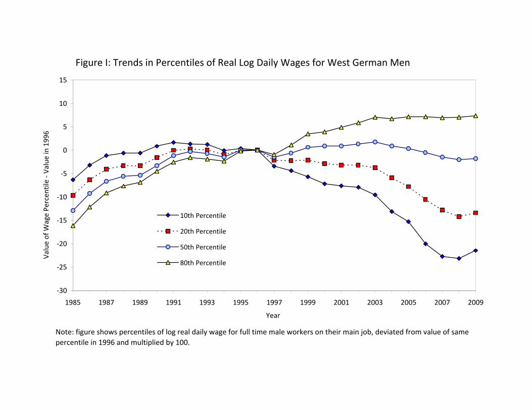
Figure I: Trends in Percentiles of Real Log Daily Wages for West German Men

‐30

‐25

‐20

‐15

‐10

‐5

0

5

10

15

1985 1987 1989 1991 1993 1995 1997 1999 2001 2003 2005 2007 2009

Year

Value of W

age Pe

rcen

tile ‐ V

alue

in 199

6

10th Percentile

20th Percentile

50th Percentile

80th Percentile

Note: figure shows percentiles of log real daily wage for full time male workers on their main job, deviated from value of samepercentile in 1996 and multiplied by 100.

Figure II: Trends in Wage Inequality for Full Time Male Workers

0.25

0.30

0.35

0.40

0.45

0.50

0.55

0.60

1985 1987 1989 1991 1993 1995 1997 1999 2001 2003 2005 2007 2009Year

Measures of Dispe

rsion

Std. Dev. of Log Wages (with Imputations)

Normalized 80‐50 Gap (Upper Tail)

Normalized 80‐20 Gap

Normalized 50‐20 Gap (Lower Tail)

Notes: figure shows measures of dispersion in real daily wage for full time male workers. Normalized percentile gaps are differences in percentiles divided by corresponding differences in percentiles of standard normal variate.

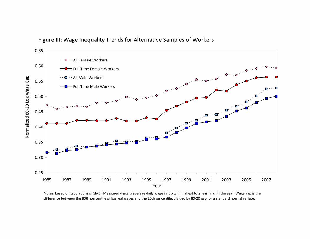
Figure III: Wage Inequality Trends for Alternative Samples of Workers

0.25

0.30

0.35

0.40

0.45

0.50

0.55

0.60

0.65

1985 1987 1989 1991 1993 1995 1997 1999 2001 2003 2005 2007Year

Normalized

80‐20

Log

Wage Gap

All Female Workers

Full Time Female Workers

All Male Workers

Full Time Male Workers

Notes: based on tabulations of SIAB . Measured wage is average daily wage in job with highest total earnings in the year. Wage gap is the difference between the 80th percentile of log real wages and the 20th percentile, divided by 80‐20 gap for a standard normal variate.

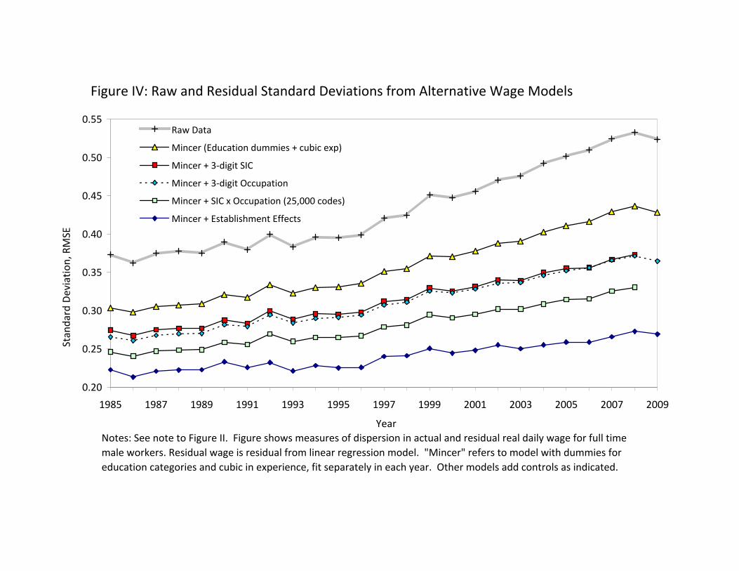
Figure IV: Raw and Residual Standard Deviations from Alternative Wage Models

0.20

0.25

0.30

0.35

0.40

0.45

0.50

0.55

1985 1987 1989 1991 1993 1995 1997 1999 2001 2003 2005 2007 2009

Year

Standard Deviatio

n, RMSE

Raw Data

Mincer (Education dummies + cubic exp)

Mincer + 3‐digit SIC

Mincer + 3‐digit Occupation

Mincer + SIC x Occupation (25,000 codes)

Mincer + Establishment Effects

Notes: See note to Figure II. Figure shows measures of dispersion in actual and residual real daily wage for full time male workers. Residual wage is residual from linear regression model. "Mincer" refers to model with dummies for education categories and cubic in experience, fit separately in each year. Other models add controls as indicated.

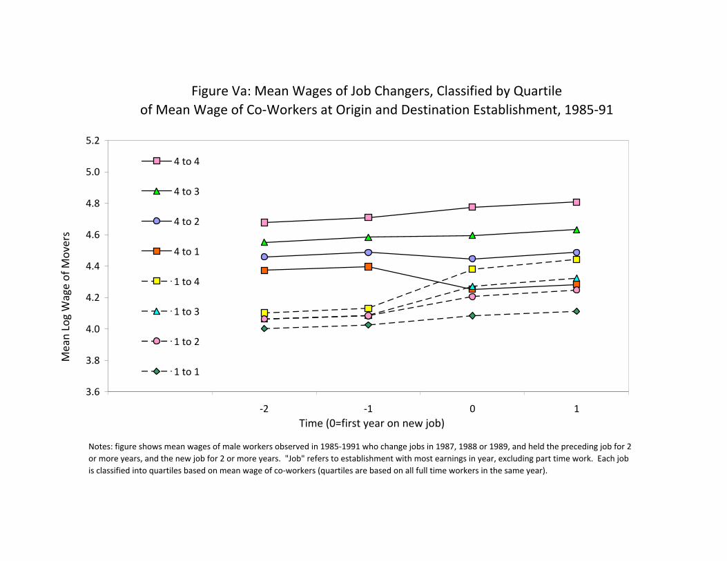
Figure Va: Mean Wages of Job Changers, Classified by Quartile of Mean Wage of Co‐Workers at Origin and Destination Establishment, 1985‐91

3.6

3.8

4.0

4.2

4.4

4.6

4.8

5.0

5.2

‐2 ‐1 0 1Time (0=first year on new job)

Mean Log Wage of M

overs

4 to 4

4 to 3

4 to 2

4 to 1

1 to 4

1 to 3

1 to 2

1 to 1

Notes: figure shows mean wages of male workers observed in 1985‐1991 who change jobs in 1987, 1988 or 1989, and held the preceding job for 2 or more years, and the new job for 2 or more years. "Job" refers to establishment with most earnings in year, excluding part time work. Each job is classified into quartiles based on mean wage of co‐workers (quartiles are based on all full time workers in the same year).

Figure Vb: Mean Wages of Job Changers, Classified by Quartile of Mean Wage of Co‐Workers at Origin and Destination Establishment, 2002‐09

3.6

3.8

4.0

4.2

4.4

4.6

4.8

5.0

5.2

‐2 ‐1 0 1Time (0=first year on new job)

Mean Log Wage of M

overs

4 to 4

4 to 3

4 to 2

4 to 1

1 to 4

1 to 3

1 to 2

1 to 1

Notes: figure shows mean wages of male workers observed in 2002‐2009 who change jobs in 2004‐2007 and held the preceding job for 2 or more years, and the new job for 2 or more years. "Job" refers to establishment with most earnings in year, excluding part time work. Each job is classified into quartiles based on mean wage of co‐workers (quartiles are based on all full time workers in the same year).

1 2 3 4 5 6 7 8 9 10

1

4

7

10

‐0.02

‐0.01

0.00

0.01

0.02

0.03

Mean Re

sidu

al

1 2 3 4 5 6 7 8 9 10

1

4

7

10

Establishment Effect Decile

Person Effect Decile

Figure VI: Mean Residual by Person/Establishment Deciles, 2002‐09

Notes: figure shows mean residuals from estimated AKM with cells defined by decile of estimated establishment effect, interacted with decile of estimated person effect. See column 4 of Table III for summary of model parameters.

Figure VII: Mean Wages of Movers, Classified by Quartile of Establishment Effects for Origin and Destination Firms, 2002‐2009

3.6

3.8

4.0

4.2

4.4

4.6

4.8

5.0

5.2

‐2 ‐1 0 1Time (0=first year on new job)

Mean Log Wage of M

overs

4 to 4

4 to 3

4 to 2

4 to 1

1 to 4

1 to 3

1 to 2

1 to 1

Notes: figure shows mean wages of male workers observed in 2002‐2009 who change jobs in 2004‐2007, and held the preceding job for 2 or more years, and the new job for 2 or more years. "Job" refers to main job in year, excluding part time jobs. Each job is classified into quartiles based on estimated establishment effect from AKM model presented in Table IIII column 4.

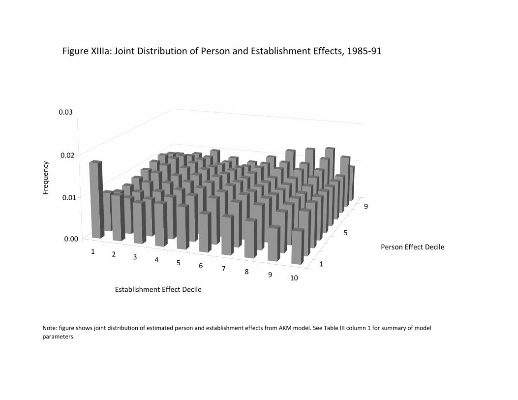
1 2 3 4 5 6 7 8 9 10

1

5

9

0.00

0.01

0.02

0.03

Freq

uency

Establishment Effect Decile

Person Effect Decile

Figure XIIIa: Joint Distribution of Person and Establishment Effects, 1985‐91

Note: figure shows joint distribution of estimated person and establishment effects from AKM model. See Table III column 1 for summary of model parameters.

1 2 3 4 5 6 7 8 9 10

1

4

7

10

0.00

0.01

0.02

0.03

Freq

uency

Establishment Effect Decile

Person Effect Decile

Figure XIIIb: Joint Distribution of Person and Establishment Effects, 2002‐09

Note: figure shows joint distribution of estimated person and establishment effects from AKM model. See Table III column 4 for summary of model parameters.

Figure IX: Standard Deviation of Establishment Effects and Fraction Covered by Collective Agreements, by Birth Year of Establishment

0.10

0.20

0.30

0.40

0.50

0.60

0.70

1985 1989 1993 1997 2001 2005 2009

First Year of Observation in IAB

Standard Deviatio

n, Coverage Ra

te

Fraction Covered(1999‐2008 LIAB)

Std. Dev. ofEstabl. Effects in1985‐91

Std. Dev. ofEstabl. Effects in1990‐1996

Std. Dev. ofEstabl. Effects in1996‐2002

Std. Dev. ofEstabl. Effects in2002‐2009

Notes: figure shows standard deviation of estimated establishment effects in a given observation interval (1985‐ 1991, 1990‐1996, 1996‐2002, or 2002‐2009) for establishments that are present in that interval and first appeared with positive full time male employment in the IEB data in the "birth year" indicated on the x‐axis. Figure also shows fraction of establishments in a given birth year surveyed in the 1999‐2008 LIAB that are covered by collective agreements.

Figure X: Distribution of Establishment Effects by Collective Bargaining Status(Based on Establishment Effects for 1996‐2002, Bargaining Status in 2000 LIAB)

0.00

0.05

0.10

0.15

0.20

0.25

0.30

1 2 3 4 5 6 7 8 9 10Establishment Effect Decile

Fractio

n in Decile

In Sectoral Agreement

Firm‐specific Contract

No Collective Bargain

Note: figure shows distribution of collective bargaining coverage status (no collective bargain, covered by firm‐specific agreement, or covered by sectoral agreement) for 7,080 establishments in 2000 Wave of LIAB that can be linked to IEB data. Establishments are classified into deciles of their estimated establishment effects from AKM model fit to 1996‐2002 data.

Online Appendix to Card, Heining, and Kline (2013)

January 29, 2013

Contents

1 Sample Construction and Processing 11.1 Creation of Wage Data . . . . . . . . . . . . . . . . . . . . . . . . . . . . . . 11.2 Education . . . . . . . . . . . . . . . . . . . . . . . . . . . . . . . . . . . . . 21.3 Occupation and Industry . . . . . . . . . . . . . . . . . . . . . . . . . . . . . 21.4 Tobit imputations . . . . . . . . . . . . . . . . . . . . . . . . . . . . . . . . . 31.5 Validation Exercise . . . . . . . . . . . . . . . . . . . . . . . . . . . . . . . . 4

2 Computational Methods 5

3 Bias in the estimated covariance matrix of person and establishment ef-fects 6

4 Appendix Figures and Tables 8

In this appendix, we provide additional details on the construction of our sample, the

nature of our imputation procedure, and provide some supplementary results.

1 Sample Construction and Processing

1.1 Creation of Wage Data

Our basic data source is the Integrated Employment Biography (IEB) database. The IEB

consists of information on employment spells at a given establishment (or firm) within a

calendar year, taken from notices of employment filed by the employer. Each notice of

employment has a beginning date (e.g., January 1), an end date (e.g., December 31), the

average daily wage earned by the employee (censored at the Social Security maximum earn-

ings level), indicators for the legal status of the job (including whether the job is full time or

part time and whether the job is a “marginal job”subject to reduced Social Security taxes),

1

as well as information on the gender, birth date, educational qualification and occupation of

the worker, and the industry and geographic location of the establishment.

We process the data in two steps. First, we collapse all spells that are recorded as full-

time jobs at the same employer in a given year into a single person-firm-year record, summing

total earnings at each employer. Row 1 of panels A and B in Appendix Table A.1 shows the

numbers of spell records in the IAB data file for full-time male and female employees age

20-60 working in non-marginal jobs in 1985 (the first year of our sample), 1997 (the middle

year of our sample) and 2009 (the last year). Row 2 in each panel shows the number of

person-firm-year records: on average there are about 1.06 spells per person-firm-year in the

early years of our sample, rising slightly to 1.11 spells per person-firm-year in 2009 (see row

4).

In the second step we select one observation per person per year by selecting the person-

firm record with the highest total earnings in a given year (and excluding any observation

with a daily wage < 10 Euros). On average each person has about 1.1 different employers

per year, with only a small upward trend over our sample period (see row 5 in each panel).

Line 3 in panels A and B shows the numbers of person-year observations for full time men

and women in our final data set.

1.2 Education

Education levels in the IEB are coded into 6 categories, plus a missing or undetermined cate-

gory. We group these into 5 classes: (1) missing; (2) primary/lower secondary or intermediate

school leaving certificate, or equivalent, with no vocational qualification; (3) primary/lower

secondary or intermediate school leaving certificate, or equivalent, with a vocational qual-

ification; (4) upper secondary school certificate (“Arbitur”) with or without a vocational

certificate; (5) degree from Fachhochschule or university. For simplicity we refer to the third

category as “apprentices”and the fifth category as “university graduates”. For an individual

who is observed in multiple notifications from the same employer in the same year we assign

the highest education category for that person-firm-year observation. Within each job spell

we assign the modal education category observed for an individual in the years he is at the

same job.

1.3 Occupation and Industry

In the IEB data, each job notification includes information on occupation and industry.

For an individual who is observed in multiple notifications from the same employer in the

same year we assign the highest occupation category and the highest industry category for

2

that person-firm-year observation. Within job spells the industry code is constant in 97%

of spells. In the remaining cases we assign the highest industry category observed over the

years of the job. We do not assign a fixed occupation code to job spells.

1.4 Tobit imputations

As illustrated in Table I of the paper, roughly 10 percent of person-year observations for male

workers and 1-2 percent of the observations for female workers are censored at the Social

Security maximum. We follow Dustmann, Ludsteck, and Schönberg [2009] and fit a series

of Tobit models to log daily wages. We then impute an uncensored value for each censored

observation using the estimated parameters of these models and a random draw from the

associated (left- censored) distribution.1

Since we are fitting models that include both a person and year effect, we want the

imputation model to reflect individual and job-specific components of the wage. We therefore

construct, for each individual in each year, the mean of his log wage in all other periods,

and the fraction of other years that the individual’s wage is censored. For individuals who

are only observed in one year, we set the mean log wage in other years to the sample mean,

and the fraction of censored wages in other years equal to the sample mean, and include a

dummy in the model for those who are observed only once. We also construct the mean log

wage for the individual’s co-workers in the current year (i.e., the “leave out mean”of log

wages at his employer) and the fraction of co-workers who are censored in the current year

(the “leave out mean”of the censoring rate at his employer). For individuals who work at an

establishment with only 1 full time male employee we set the mean log wage for co-workers

equal to the sample mean, and the fraction of co-workers with censored wages equal to the

sample mean, and include a dummy in the model for employees of 1-worker firms.

We then fit a series of 500 Tobit models separately by year, education (5 values: missing;

no qualification; apprenticeship; some post secondary; and university graduate), and 10 year

age range (20-29; 30-39; 40-49; 50-60), including the following variables: age, mean log wage

in other years, fraction of censored wages in other years, number of full time male employees

at the current firm and its square, dummy for 11 or more employees, mean years of schooling

and fraction of university graduates at the current firm, mean log wage of co-workers and

fraction of co-workers with censored wages, dummy for individuals observed only 1 year

between 1985 and 2009, dummy for employees of 1-worker firm. Appendix Table A.2 shows

1Specifically, we impute an upper tail as follows. Suppose that the estimated Tobit model for y (the logof wages) has y ∼ N(X ′β, σ), and consider a censored observation, such that y ≥ c, where c is the censoringpoint. Let k = Φ[(c−X ′β)/σ], where Φ represents the standard normal density, and let u ∼ U [0, 1] representa uniform random variable. Then we impute an uncensored value for y as: yu = X ′β+σΦ−1[k+u× (1−k)].

3

the coeffi cient estimates for models for 40-49 year old apprentices in 1985, 1997, and 2009.

1.5 Validation Exercise

To evaluate the quality of the approximation to the upper tail provided by our Tobit speci-

fication, we performed a validation exercise in which we artificially censor the upper tail of

wages for a group of workers with very low censoring rates, then fit Tobit models (with the

same explanatory variables as in our main procedure) and stochastically impute the upper

tail of wages. We then compare the standard deviation of wages for the original sample with

the standard deviation from the censored/imputed sample. We use male workers age 20-29

with an apprenticeship education in years from 1990 to 2009 as the population of interest.

These workers have an average censoring rate over the 20 year period of 0.7%. We select

artificial censoring points so that 10, 20, 30, or 40 percent of workers are censored in each

year, and fit separate Tobit models by year for each censored subsample.

Appendix Figure A.1 shows actual standard deviation of wages for the test sample, which

rises from 0.296 to 0.348 (an increase of 0.052) between 1990 and 2009, as well as the standard

deviations from the censored/imputed samples with differing censoring rates. The standard

deviation of the imputed series is uniformly higher than the standard deviation of the raw

data, with a larger upward bias at higher censoring rates. For example, when the censoring

rate is 40%, the estimated standard deviation is upward biased by about 0.04 (or 13%) in

every year. Fortunately, the upward bias is relatively constant, so the trend in the dispersion

of wages is very similar whether we use the raw data or any of the censored/imputed series.

This leads us to conclude that our Tobit imputation procedure performs relatively well, even

for subgroups with very high censoring rates.

A concern about our imputation procedure is that it may alter the relative share within

versus between establishment variation. To check this, we fit linear regression models with

year dummies and establishment effects to observations from 2002 to 2009 (the same time

span as our fourth sample interval), using the raw wage data for 20-29 year old men with an

apprenticeship education, and the censored/imputed data. The sample has 8,426,930 person-

year wage observations on employees at 668,285 establishments. The R-squared coeffi cients

from the different samples were as follows:

raw data: 0.721

10% censored 0.719

20% censored 0.718

30% censored 0.714

40% censored 0.707

4

We conclude that the imputation procedure successfully maintains the relative share

of the variance of wages attributable to within-establishment variation, even at very high

censoring rates.

2 Computational Methods

Because our dataset is very large and identification of the establishment effects derives en-

tirely frommovers, we conducted estimation in two steps. First, in each interval, we extracted

the sample of workers who switched establishments over the relevant time period. We fit the

model to this sample of movers and recovered the estimated vector of establishment effects

ψ along with the coeffi cients β corresponding to the time varying covariates xit.2 Then, for

each worker who stayed at the same establishment over the sample interval, we computed

an estimate of his person effect as follows:

αi =1

Ti

∑t

(yit − ψJ(i,t) − x′itβ

)where Ti is the number of periods that individual i is observed in the sample interval. Our

root mean squared error calculations were conducted by reducing the degrees of freedom by

one for each connected stayer mean estimated.3

Our estimation tasks were performed in Matlab. Code for our analysis is available on-

line. We used a variant of the depth first search algorithm implemented in the open source

matlabBGL package to find the largest connected set of establishments in each data inter-

val. The design matrices Z ≡ [D,F,X] were stored as sparse matrices. To compute the

least squares solutions we solved the normal equations in equation (3) of the paper using

Matlab’s preconditioned conjugate gradient routine (see Shewchuck [1994] for a lucid intro-

duction). To speed the process we used an incomplete Cholesky factorization of Z ′Z as the

preconditioner with threshold dropping tolerance of 0.01.

2This yields an ineffi cient estimator of β. However, in a sample of roughly 90 million observations, precisionis not a major concern. A separate issue is that our two step procedure only ensures orthogonality betweenthe AKM residuals rit and xit in the sample of movers. In practice, the correlation in the sample ofestablishment stayers between x′itβ and the AKM residuals is very small in each interval, with the largestcorrelation occuring in interval 3 and amounting to approximately −.01.

3That is we used the formula RMSE =√

SSRdof where SSR is the sum of squared residuals across all

person-year observations in the interval and dof = N∗ −N − (J − 1)− rank (X), where N∗ is the numberof person year observations including the stayers, N is the number of connected individuals including thestayers, and J is the number of connected establishments.

5

3 Bias in the estimated covariance matrix of person

and establishment effects

It is well known that sampling errors in the estimated person and establishment effects may

lead to inflated estimates of the standard deviation of each component and negatively biased

estimates of the covariance between the person and establishment effects. This has led some

authors (e.g., Andrews et al., 2008) to propose parametric bias corrections to the estimated

components. To illustrate the logic of such an approach, and the diffi culties involved, we

denote the population quantities of interest as:

σ2Dα ≡ 1

N∗ − 1α′D′Q1Dα (Variance of person effects)

σ2Fψ ≡ 1

N∗ − 1ψ′F ′Q1Fψ (Variance of establishment effects)

σDα,Fψ ≡ 1

N∗ − 1ψ′F ′Q1Dα (Covariance of person and establishment effects)

where Q1 ≡ I − 1 (1′1)−1 1′ is a symmetric demeaning matrix.

OLS estimation of (2) yields a coeffi cient vector:

ξ = ξ + (Z ′Z)−1Z ′r

with E[(Z ′Z)−1 Z ′r

]= 0. The sampling variance of this vector can be written:

Vξ ≡ E

[(ξ − ξ

)(ξ − ξ

)′]= (Z ′Z)

−1Z ′ΩZ (Z ′Z)

−1

where Ω ≡ E [rr′] is the N∗ ×N∗ variance covariance matrix of the errors.

The sample analogues to the population quantities can be expressed in terms of the

following quadratic forms:

σ2Dα ≡ 1

N∗ − 1ξ′ADαξ

σ2Fψ ≡ 1

N∗ − 1ξ′AFψ ξ

σDα,Fψ ≡ 1

N∗ − 1ξ′ADα,Fψ ξ

6

where ADα ≡

D′Q1D 0 0

0 0 0

0 0 0

, AFψ ≡ 0 0 0

0 F ′Q1F 0

0 0 0

, ADα,Fψ ≡ 0 F ′Q1D 0

0 0 0

0 0 0

.Unbiasedness of OLS and standard results on quadratic forms imply that for any matrix

A,

E[ξ′Aξ]

= ξ′Aξ + tr(AVξ

).

Therefore the bias in our estimates of the variance components corresponds to the trace

term in the above expression, which in turn depends critically upon Vξ. Previous work has

focused on evaluating this bias expression under the assumption that the r are independent

and identically distributed in which case Ω = Iσ2 and Vξ = (Z ′Z)−1 σ2.

Unfortunately, the bulk of the literature on earnings dynamics (MaCurdy, 1982; Abowd

and Card, 1989; Meghir and Pistaferri, 2004) suggests a substantially more complicated error

structure of earnings with complex forms of temporal dependence and heteroscedasticity.

Errors in modeling the structure of Ω will induce errors in estimation of Vξ which is why, at

least since the work of White [1980], economists have sought robust variance estimates that

don’t rely upon estimation of all elements of Ω. Unfortunately, robust variance estimation

is not possible in our setting because the estimates ξ, while unbiased, are not consistent.

In unreported results we have attempted parametric corrections allowing for a match

component and a moving average component to the errors r. These corrections yielded

small changes in the estimated variance-covariance matrix Vξ and had trivial effects on the

trends of the various components. In sampling experiments we found the corrections to

provide a poor guide to the degree of bias created by working with subsamples of the data.

We suspect this is because our model for the errors is insuffi ciently rich — a problem we

are unlikely to be able to solve in a convincing way. For this reason, our decompositions in

section 7 of between group means are of particular interest because these results are based

upon group averages involving tens of thousands (or in some cases millions) of observations,

in which case biases due to sampling error become largely irrelevant.

References

Abowd, John and David Card. 1989. “On the Covariance Structure of Earnings and

Hours Changes.”Econometrica 57(2): 411-445.

Andrews, M.J., L. Gill, T. Schank, and R. Upward. 2008. “High wage workers and low

wage firms: negative assortative matching or limited mobility bias?”Journal of the Royal

Statistical Society 171(3): 673-679.

7

Dustmann, Christian, Johannes Ludsteck, and Uta Schönberg. 2009. “Revisiting the

German Wage Structure.”Quarterly Journal of Economics 124(2): 843-881.

Macurdy, Thomas. 1982. “The use of time series processes to model the error structure

of earnings in a longitudinal data analysis.”Journal of Econometrics 18(1): 83-114.

Meghir, Costas and Luigi Pistaferri. 2004. “Income Variance Dynamics and Heterogene-

ity.”Econometrica 72(1): 1-32.

Shewchuck, Jonathan Richard. 1994. “An Introduction to the Conjugate Gradient

Method Without the Agonizing Pain: Edition 114”Working paper. School of Computer

Science, Carnegie Mellon University.

White, Halbert. 1980. “A heteroskedasticity-consistent covariance matrix and a direct

test for heteroskedasticity.”Econometrica 48(4): 817—838.

4 Appendix Figures and Tables

8

Appendix Figure A.1: Trends in Standard Deviations of Log Wages ‐ Male Apprentices Age 20‐29, Actual and Artificially Censored/Imputed Data

0.27

0.29

0.31

0.33

0.35

0.37

0.39

0.41

1990 1992 1994 1996 1998 2000 2002 2004 2006 2008

Standard Deviatio

n

40% Censored with Tobit Imputations: Rise=0.054

30% Censored with Tobit Imputations: Rise=0.055

20% Censored with Tobit Imputations: Rise=0.056

10% Censored with Tobit Imputations: Rise=0.054

Actual Data: Rise=0.052

Note: Actual data has censoring rate of 0.5% or less in every year. Data are artificially censored at real wages levels yielding average censoring rates of 10,20,30, or 40% over the entire sample period. Then Tobit models are fit separately by year, with same covariates as used in main imputation model, and upper tail observations are randomly imputed using same procedure as in main imputation model.

Appendix Figure A.2: Raw and Residual Standard Deviations from Alternative Wage Models for Full Time Females

0.25

0.30

0.35

0.40

0.45

0.50

0.55

0.60

0.65

1985 1987 1989 1991 1993 1995 1997 1999 2001 2003 2005 2007 2009

Year

RMSE

Raw Data

Mincer (Education dummies + cubic exp)

Mincer + 3‐digit SIC

Mincer + 3‐digit Occupation

Mincer + SIC x Occupation (25,000 codes)

Mincer + Establishment Effects

Notes: See notes to Figure IV. Figure shows measures of dispersion in actual and residual real daily wage for full time female workers. Residual wage is residual from linear regression model. "Mincer" refers to model with dummies for education categories and cubic in experience, fit separately in each year. Other models add additional controls as indicated.

Appendix Table A.1: Job Spells and Main Jobs in IEB Data Base

1985 1997 2009

A. Male Workers

1. Number of Full Time Job Spells 13,987,548 14,919,079 14,911,559 (age 20‐60, non‐marginal jobs)

2. Number of unique person‐firm‐ 13,181,917 13,968,286 13,456,305 year observations

3. Number of person‐year observations 11,980,159 12,661,995 12,104,223 (highest‐paying job only)

4. Average number of spells per 1.06 1.07 1.11 job in year

5. Average number of jobs per year 1.10 1.10 1.11

B. Female Workers1. Number of Full Time Job Spells 6,965,926 7,937,037 8,142,682 (age 20‐60, non‐marginal jobs)

2. Number of unique person‐firm‐ 6,642,114 7,408,237 7,328,008 year observations

3. Number of person‐year observations 6,068,863 6,758,622 6,566,429 (highest‐paying job only)

4. Average number of spells per 1.05 1.07 1.11 job in year

5. Average number of jobs per year 1.09 1.10 1.12Notes: each "job spell" represents a notification of employment in the IEB data base. For each gender, the entry in row 1 is the number of such notifications for full time, non‐marginal jobs held by men age 20‐60. Row 2 shows the number of unique person‐firm‐year observations after collapsing multiple spells at the same employer in the same year. Row 3 shows the number of person observations after selecting the person‐firm‐year observation with the highest total earnings in the year as the "main job" in a given year. Row 4 gives the ratio of row 1 to row 2. Row 5 gives the ratio of row 2 to row 3.

Appendix Table A.2: Selected Tobit Models for Male Apprentices, Age 40‐49

1985 1997 2009Moments of Unadjusted Log Wage Data: Mean 4.382 4.4612 4.434

Std. Deviation 0.2677 0.3104 0.3563

Fraction Censored 0.155 0.107 0.0726

Parameter Estimates from Tobit model: Intercept 0.539 ‐0.108 ‐0.194

(0.030) (0.020) (0.003) Age/10 0.026 ‐0.009 ‐0.103

(0.002) (0.002) (0.003) Fraction of person's other wage 0.268 0.270 0.699 observations censored (0.003) (0.005) (0.011) Mean of log wage for person 0.693 0.909 0.819 in other years (0.003) (0.003) (0.004) Dummy for firm size > 10 ‐0.006 ‐0.006 0.005

(0.002) (0.002) (0.002) Fraction of workers at firm with ‐0.045 ‐0.013 0.007 university degree* (0.012) (0.011) (0.014) Mean years of schooling of workers ‐0.014 ‐0.010 ‐0.007 at firm* (0.002) (0.002) (0.002) Fraction of co‐workers with 0.093 0.000 0.135 censored wage** (0.007) (0.007) (0.010) Mean log wage of co‐workers** 0.187 0.163 0.374

(0.004) (0.004) (0.004) Dummy if person observed in ‐0.398 ‐0.935 ‐0.808 only 1 year (0.005) (0.013) (0.016) Dummy if firm has only 1 ‐0.223 ‐0.178 ‐0.386 worker (0.005) (0.005) (0.006)

Estimated scale parameter 0.147 0.135 0.195(0.001) (0.001) (0.001)

Sample size 62,889 58,392 65,904

Notes: standard errors in parentheses. Table entries are coefficient estimates from Tobit models fit to log real daily wages, with censoring at the Social Security maximum contribution rate. Models also include firm size (number of current‐year full time male employees) and its square.

*Characteristics of full‐time male (non‐marginal) employees at the same firm.

**Statistic is calculated for full‐time male employees at the same firm, excluding the individual of interest. For employers with one firm, statistic is set to mean.

Number of 2 Years 1 Year 1 Year 2 Years Origin/destination Observations: Before Before After After Raw Adjusted**

Quartile* (1) (2) (3) (4) (5) (6) (7)

Interval 1: 1985‐19911 to 1 333,648 4.00 4.03 4.08 4.11 0.11 0.001 to 2 206,251 4.06 4.08 4.21 4.25 0.18 0.071 to 3 136,119 4.06 4.09 4.27 4.32 0.26 0.151 to 4 82,193 4.10 4.13 4.38 4.44 0.34 0.23

2 to 1 125,376 4.16 4.18 4.14 4.18 0.01 ‐0.072 to 2 204,787 4.23 4.25 4.29 4.32 0.09 0.002 to 3 158,360 4.26 4.28 4.36 4.40 0.14 0.052 to 4 86,038 4.30 4.32 4.47 4.53 0.23 0.14

3 to 1 59,334 4.25 4.26 4.16 4.19 ‐0.05 ‐0.153 to 2 91,474 4.32 4.34 4.33 4.37 0.06 ‐0.053 to 3 173,160 4.38 4.41 4.45 4.49 0.10 0.003 to 4 136,569 4.46 4.49 4.59 4.64 0.18 0.07

4 to 1 30,110 4.37 4.40 4.25 4.28 ‐0.09 ‐0.224 to 2 41,079 4.46 4.49 4.45 4.49 0.03 ‐0.104 to 3 91,177 4.55 4.58 4.60 4.63 0.08 ‐0.054 to 4 290,921 4.68 4.71 4.78 4.81 0.13 0.00

Interval 4: 2002‐20091 to 1 541,307 3.88 3.87 3.87 3.88 0.00 0.001 to 2 197,982 4.02 4.02 4.17 4.18 0.16 0.171 to 3 88,768 4.00 4.02 4.29 4.32 0.33 0.331 to 4 49,167 4.06 4.08 4.47 4.52 0.47 0.47

2 to 1 208,184 4.20 4.19 4.02 4.03 ‐0.17 ‐0.162 to 2 333,219 4.32 4.31 4.30 4.31 ‐0.01 0.002 to 3 137,528 4.38 4.38 4.44 4.46 0.08 0.082 to 4 59,080 4.47 4.48 4.63 4.67 0.20 0.21

3 to 1 73,218 4.34 4.33 4.02 4.04 ‐0.30 ‐0.313 to 2 133,606 4.46 4.46 4.39 4.40 ‐0.06 ‐0.073 to 3 275,521 4.55 4.55 4.56 4.57 0.02 0.003 to 4 150,989 4.68 4.69 4.77 4.81 0.13 0.11

4 to 1 32,664 4.52 4.53 4.14 4.17 ‐0.35 ‐0.434 to 2 47,193 4.65 4.67 4.53 4.56 ‐0.09 ‐0.184 to 3 127,276 4.74 4.76 4.72 4.75 0.00 ‐0.084 to 4 546,855 4.94 4.96 4.97 5.02 0.08 0.00

Appendix Table A.3: Mean Log Wages Before and After Job Change, by Quartile of Mean Co‐workers' Wages at Origin and Destination Establishments

*Quartiles are based on mean wages of co‐workers at old job in year prior to move, and in new job in year after move.**Trend‐adjusted mean wage change, calculated as mean wage change for origin‐destination group, minus mean change for job movers from the same origin quartile who remain in same quartile.

Mean Log Wages of Movers

Notes: entries are mean log real daily wages for job changers who are observed with at least 2 years of data prior to a job change, and two years after. Sample excludes movers to/from establishments with 1 worker.

Change from 2 Years Before to 2 Years After:

Appendix Table A.4: Estimation Results for AKM Model, Fit by Interval for Male ApprenticesInterval 1 Interval 2 Interval 3 Interval 41985‐1991 1990‐1996 1996‐2002 2002‐2009

(1) (2) (3) (4)Person and Establishment Parameters: Number person effects 10,128,342 10,346,742 9,288,956 8,145,059

Number establishment effects 1,008,959 1,078,911 1,093,438 990,608

Summary of Parameter Estimates: Std. dev. of person effects 0.241 0.249 0.271 0.285 (across person‐year obs.)

Std. dev. of establ. effects 0.152 0.159 0.170 0.202 (across person‐year obs.)

Std. dev. of Xb 0.121 0.080 0.073 0.064 (across person‐year obs.)

Correlation of person/est effects ‐0.035 0.008 0.048 0.098 (across person‐year obs.)

Correlation of person effects/Xb 0.050 0.075 ‐0.029 0.020 (across person‐year obs.)

Correlation of establ. effects/Xb 0.064 0.064 0.048 0.082 (across person‐year obs.)

RMSE of AKM residual 0.110 0.109 0.110 0.110

Adjusted R‐squared 0.887 0.891 0.901 0.919

Comparison Match Model RMSE of Match model 0.096 0.095 0.094 0.094

Std. Dev of Match Effect* 0.054 0.052 0.056 0.057

Std. Dev. Log Wages 0.328 0.329 0.349 0.388

Sample size 54,993,845 56,701,812 51,031,280 50,700,611

Notes: see notes to Table III. Models reported here are estimated for subsample of full time male workers with apprenticeship training only. Xb includes year dummies and quadratic and cubic terms in age (total of 8 parameters in intervals 1‐3, 9 in interval 4). Match model includes Xb and separate dummy for each job (person‐establishment pair).*Standard deviation of match effect estimated as square root of difference in mean squared errors between AKM model and match effect model.

Appendix Table A.5: Decompositions of Rise in Wage Inequality for Apprentices

Var. Component Share of Total Var. Component Share of Total Var. Component Share of Total(1) (2) (3) (4) (5) (6)

Total variance of log wages 0.108 100.0 0.150 100.0 0.043 100

Components of Variance:

Variance of person effect 0.058 53.7 0.081 54.2 0.024 55

Variance of establ. effect 0.023 21.3 0.041 27.1 0.018 42

Variance of Xb 0.015 13.6 0.004 2.7 ‐0.011 ‐25

Variance of residual 0.010 8.9 0.010 6.6 0.000 1

2cov(person, establ.) ‐0.003 ‐2.4 0.011 7.5 0.014 32

2cov(Xb, person+establ.) 0.005 4.9 0.003 1.9 ‐0.002 ‐6

Counterfactuals for Variance of log wages: *

1. No rise in correl. of person/estab. effect 0.108 0.143 0.035 82

2. No rise in var. of estab. effect 0.108 0.131 0.023 55

3. Both 1 and 2 0.108 0.125 0.018 42

*Counterfactual 1 computes the counterfactual rise in variance assuming the correlation between the person and establishment effects remains at its

interval 1 value ‐‐ i.e. imposing the restriction that Cov4(person, establ.) = ρ1 Var4(person)1/2 x Var4(establ.)

1/2 where subscript 4 refers to the interval 4 value of the statistic and and ρ1 is the correlation between the person and establishment effects in interval 1. Counterfactual 2 assumes that the variance of establishment effects remains at its interval 1 level. Counterfactual 3 imposes both of these restrictions.

Interval 1 (1985‐1991) Interval 4 (2002‐2009)

Notes: see notes to Table IV. Calculations based on estimated AKM models summarized in Appendix Table A.4.

Change from Interval 1 to 4

Appendix Table A.6: Estimation Results for AKM Model for Full Time Female WorkersInterval 1 Interval 2 Interval 3 Interval 41985‐1991 1990‐1996 1996‐2002 2002‐2009

(1) (2) (3) (4)Person and Establishment Parameters: Number person effects 9,660,968 10,155,014 9,756,379 9,559,738

Number establishment effects 1,079,129 1,176,133 1,191,607 1,196,201

Summary of Parameter Estimates: Std. dev. of person effects 0.332 0.332 0.365 0.397 (across person‐year obs.)

Std. dev. of establ. effects 0.232 0.227 0.247 0.277 (across person‐year obs.)

Std. dev. of Xb 0.145 0.098 0.086 0.087 (across person‐year obs.)

Correlation of person/establ. effects ‐0.009 0.039 0.044 0.069 (across person‐year obs.)

Correlation of person effects/Xb ‐0.249 ‐0.140 ‐0.117 ‐0.089 (across person‐year obs.)

Correlation of establ. effects/Xb 0.040 0.024 0.009 0.041 (across person‐year obs.)

RMSE of AKM residual 0.137 0.135 0.147 0.157

Adjusted R‐squared 0.894 0.900 0.901 0.909

Comparison Match Model RMSE of Match model 0.117 0.118 0.125 0.133

Adjusted R‐squared 0.922 0.924 0.928 0.934

Std. Dev. of Match Effect* 0.070 0.067 0.077 0.083

Addendum

Std. Dev. Log Wages 0.420 0.427 0.467 0.521

Sample size 40,846,416 44,351,293 41,576,298 44,751,361

*Standard deviation of match effect estimated as square root of difference in mean squared errors between AKM model and match effect model.

Notes: see notes to Table III. Models reported here are estimated for subsample of full time female workers. Xb includes year dummies and quadratic and cubic terms in age (total of 8 parameters in intervals 1‐3, 9 in interval 4). Match model includes Xb and separate dummy for each job (person‐establishment pair).

Appendix Table A.7: Decomposition of the Rise in Wage Inequality ‐‐ Full Time Females

Var. Component Share of Total Var. Component Share of Total Var. Component Share of Total(1) (2) (3) (4) (5) (6)

Total variance of log wages 0.176 100.0 0.272 100.0 0.095 100

Components of Variance:

Variance of person effect 0.110 62.6 0.158 58.1 0.048 50

Variance of establ. effect 0.054 30.6 0.077 28.2 0.023 24

Variance of Xb 0.021 11.9 0.008 2.8 ‐0.013 ‐14

Variance of residual 0.014 7.8 0.019 6.9 0.005 5

2cov(person, establ.) ‐0.001 ‐0.8 0.015 5.6 0.017 17

2cov(Xb, person+establ.) ‐0.021 ‐12.1 ‐0.004 ‐1.5 0.017 18

Counterfactuals for Variance of log wages: *

1. No rise in correl. of person/estab. effects 0.176 0.255 0.078 82

2. No rise in var. of estab. effect 0.176 0.247 0.070 74

3. Both 1 and 2 0.176 0.232 0.056 59

*Counterfactual 1 computes the counterfactual rise in variance assuming the correlation between the person and establishment effects remains at its interval 1

value ‐‐ i.e. imposing the restriction that Cov4(person, establ.) = ρ1 Var4(person)1/2 x Var4(establ.)

1/2 where the 4 subscript refers to the interval 4 value of the statistic and ρ1 is the correlation between the person and establishment effects in interval 1. Counterfactual 2 assumes that the variance of establishment effects remains at its interval 1 level. Counterfactual 3 imposes both of these restrictions.

Interval 1 (1985‐1991) Interval 4 (2002‐2009)

Notes: See notes to Table IV. Calculations based on estimated AKM models summarized in Appendix Table A.6.

Change from Interval 1 to 4