WORKSHOP ON FRONTIERS IN BENCHMARKING TECHNIQUES AND

THEIR APPLICATION TO OFFICIAL STATISTICS

7 – 8 APRIL 2005

Reusable components for benchmarking using Kalman filters

J. Palate

1.

REUSABLE COMPONENTS FOR BENCHMARKING USING KALMAN FILTERS

Jean Palate

(jean.palate@nbb.be) R&D Unit Department of Statistics

2.

TABLE OF CONTENTS

0 INTRODUCTION 3

1 TECHNOLOGY 3

2 THEORETICAL FRAMEWORK 4

2.1 Basic Univariate State space model 4 2.1.1 Definition 4 2.1.2 Filtering, smoothing and likelihood evaluation 6

2.1.2.1 Recursions for filtering 6 2.1.2.2 Recursions for (disturbance) smoothing 7

2.1.3 Likelihood evaluation 10 2.1.4 Regressors effects 10

2.1.4.1 Extended model 11 2.1.4.2 Augmented model 12

2.2 Benchmarking 13 2.2.1 Generalities 13 2.2.2 disaggregated time series model 13 2.2.3 Aggregation 14

2.2.3.1 State-space form 14 2.2.3.2 Estimation of the aggregated model 15 2.2.3.3 Logarithmic transformation 16

2.2.3.3.1 Approximated solution 16 2.2.3.3.2 Iterative solution 16

2.2.4 Practical considerations 17

3 OO-DESIGN 18

3.1 State space models 18 3.1.1 General considerations 18 3.1.2 Models hierarchy 19 3.1.3 Filtering and smoothing 19 3.1.4 Estimation 20 3.1.5 Likelihood maximisation 20

3.2 Benchmarking 21

4 APPLICATIONS 22

5 FUTURE EXTENSIONS 25

6 CONCLUDING REMARKS 25

0

3.

INTRODUCTION

Kalman filters and smoothers are powerful algorithms that provide efficient solutions to many problems in the time series domain. This is certainly the case for some benchmarking approaches. We present in this paper how we have translated the versatility of the state-space forms and of the connected algorithms into software modules (called below "library"). For the time being, our library only tackles univariate state-space series. In spite of this important restriction, it can already be applied in many useful applications. A large part of the work is devoted to the treatment of state-space forms in general. Special attention is paid to the initialisation of non stationary models, on the handling of the regression effects and on the definition of the likelihood. The theoretical developments follow the approach of Durbin and Koopman (2001, 2003). As far as benchmarking is concerned, the present library concentrates on the estimation through single regression methods. It is much in the line of the work of Proietti (2004). That choice is mainly motivated by the wish to replace existing implementations of traditional algorithms. The new solution presents more alternatives (including the estimation of log-transformed models) and several diagnostics tools. The work is on the frontier between recent statistical developments and software design; the structure of the paper reflects that duality. In the first paragraph, we briefly discuss the general technological choices necessary to ensure a high reusability. The second paragraph describes the theoretical framework; details on the different state-space representations and on the algorithms for filtering and smoothing are provided. Paragraph 3 outlines how the theory is translated into an extensible object-model. Finally two modules built on the library are briefly presented in the last paragraph. The note is written as as technical documentation of the library for advanced users. In that perspective, most of the mathematical developments and of the discussion around the statistical methods for benchmarking have been deliberately omitted. Useful information on those topics can be found in many other papers. The library and the different applications that use it can be freely dowloaded from a WEB server of the National Bank of Belgium.

1 TECHNOLOGY

The capability of reusing previous modules or of extending them to meet new situations constitutes a very important point in software development. This is of course necessary to be able to respond quickly to new needs. From the user's point of view, it is also a way to build a coherent framework for his work. Statistical algorithms must often be integrated in completely different tasks. Benchmarking, for example, can be used in batch processing of many series; it can also be embedded in semi-automated tasks like the production of Quarterly National Accounts; advanced graphical interfaces should also be available for detailed analysis, while some facilities for more complex studies like Monte Carlo experiments are an interesting feature. It is unlikely to find a single product that can respond efficiently to all those kinds of questions. However, as far as technology is concerned, object-oriented (OO) components based on standard technologies form a very interesting solution. If their underlying technology is largely accepted by the software realm, OO components can quite easily be embedded in many different environments, from commercial software to a variety of tools

4.

for in-house developments. Java is a popular solution when portability matters, while .NET becomes the norm for Windows applications. We provide implementations in both technologies, using the same object-model. It should also be stressed that, compared to other more traditional development languages like FORTRAN or C, those technologies yield much more robust solutions. The OO paradigm is often limited to data encapsulation. While this feature is extremely useful for hiding the details of an implementation and for managing its complexity, the other characteristics of OO appear at least as important once extensibility is put forward. Polymorphism allows the building of generic algorithms, based on general concepts rather than on specific cases, while inheritance allows specialisation or modification of existing implementations. These last two aspects of OO, and more specifically polymorphism permits a reasoning very close to the theoretical developments. They are widely exploited in the design of our framework on the state-space forms (SSF henceforth) and on the Kalman filters and smoothers (KF henceforth).

2 THEORETICAL FRAMEWORK

2.1 BASIC UNIVARIATE STATE SPACE MODEL

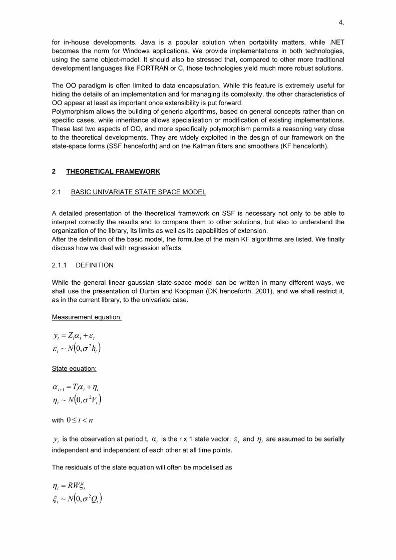
A detailed presentation of the theoretical framework on SSF is necessary not only to be able to interpret correctly the results and to compare them to other solutions, but also to understand the organization of the library, its limits as well as its capabilities of extension. After the definition of the basic model, the formulae of the main KF algorithms are listed. We finally discuss how we deal with regression effects 2.1.1 DEFINITION While the general linear gaussian state-space model can be written in many different ways, we shall use the presentation of Durbin and Koopman (DK henceforth, 2001), and we shall restrict it, as in the current library, to the univariate case. Measurement equation:

( )tt

tttt

hN

Zy2,0~ σε

εα +=

State equation:

( )tt

tttt

VN

T2

1

,0~ ση

ηαα +=+

with nt <≤0

ty is the observation at period t, is the r x 1 state vector. and tα tε tη are assumed to be serially

independent and independent of each other at all time points. The residuals of the state equation will often be modelised as

( )tt

tt

QN

RW2,0~ σξ

ξη =

5.

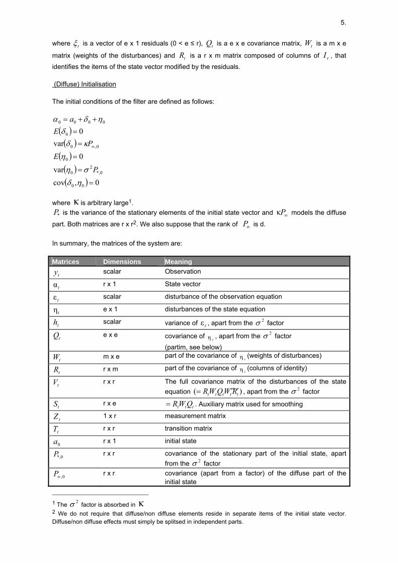
where tξ is a vector of e x 1 residuals (0 < e ≤ r), is a e x e covariance matrix, is a m x e

matrix (weights of the disturbances) and is a r x m matrix composed of columns of , that

identifies the items of the state vector modified by the residuals.

tQ tW

tR rI

(Diffuse) Initialisation The initial conditions of the filter are defined as follows:

( )( )

( )( )( ) 0,cov

var

0var

0

00

0*,2

0

0

0,0

0

0000

=

=

=

==

++=

∞

ηδση

ηκδ

δηδα

P

EP

Ea

where κ is arbitrary large1.

*P is the variance of the stationary elements of the initial state vector and models the diffuse

part. Both matrices are r x r∞Pκ

2. We also suppose that the rank of is d. ∞P In summary, the matrices of the system are: Matrices Dimensions Meaning

ty scalar Observation

tα r x 1 State vector

tε scalar disturbance of the observation equation

tη e x 1 disturbances of the state equation

th scalar variance of , apart from the factor tε2σ

tQ e x e covariance of , apart from the factor tη

2σ(partim, see below)

tW m x e part of the covariance of (weights of disturbances) tη

tR r x m part of the covariance of (columns of identity) tη

tV r x r The full covariance matrix of the disturbances of the state equation )( ttttt RWQWR ′′′= , apart from the factor 2σ

tS r x e ttt QWR= . Auxiliary matrix used for smoothing

tZ 1 x r measurement matrix

tT r x r transition matrix

0a r x 1 initial state

0*,P r x r covariance of the stationary part of the initial state, apart from the factor 2σ

0,∞P r x r covariance (apart from a factor) of the diffuse part of the initial state

1 The factor is absorbed in 2σ κ 2 We do not require that diffuse/non diffuse elements reside in separate items of the initial state vector. Diffuse/non diffuse effects must simply be splitsed in independent parts.

6.

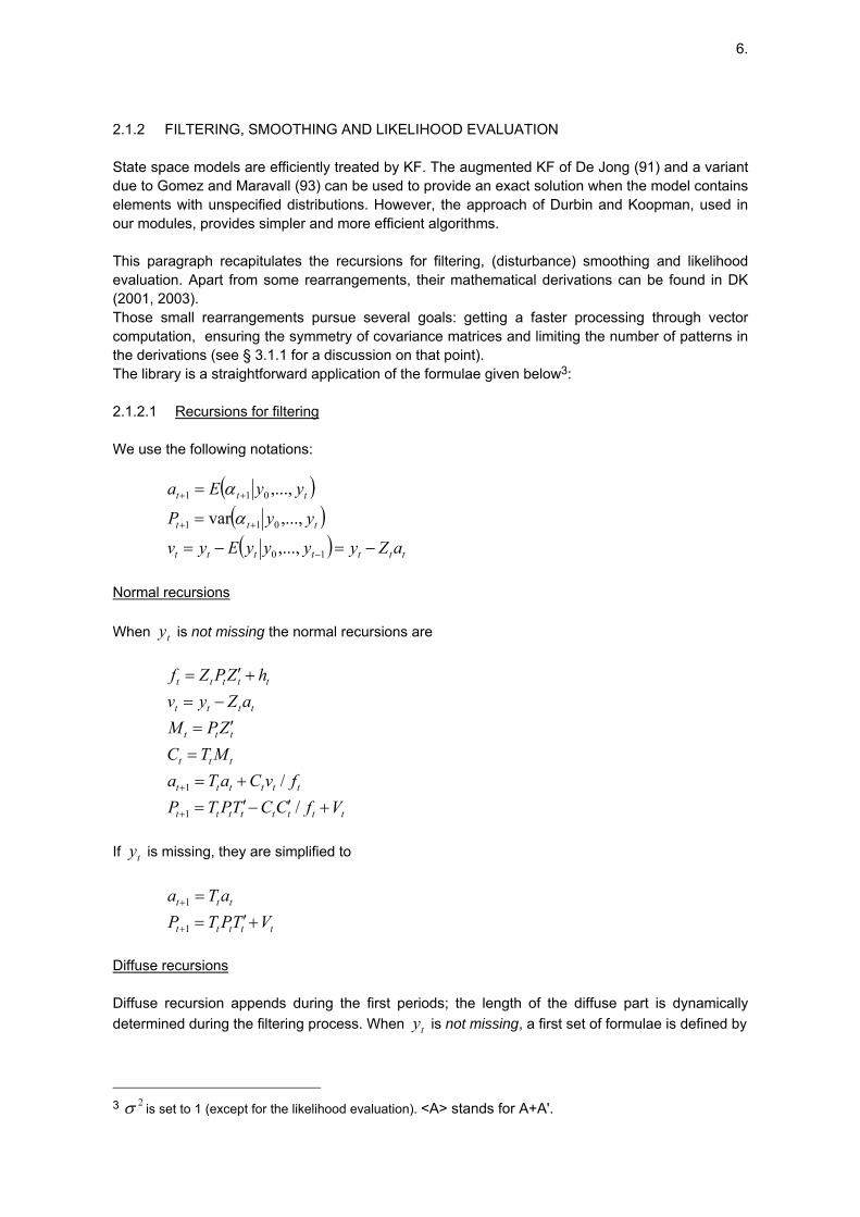
2.1.2 FILTERING, SMOOTHING AND LIKELIHOOD EVALUATION State space models are efficiently treated by KF. The augmented KF of De Jong (91) and a variant due to Gomez and Maravall (93) can be used to provide an exact solution when the model contains elements with unspecified distributions. However, the approach of Durbin and Koopman, used in our modules, provides simpler and more efficient algorithms. This paragraph recapitulates the recursions for filtering, (disturbance) smoothing and likelihood evaluation. Apart from some rearrangements, their mathematical derivations can be found in DK (2001, 2003). Those small rearrangements pursue several goals: getting a faster processing through vector computation, ensuring the symmetry of covariance matrices and limiting the number of patterns in the derivations (see § 3.1.1 for a discussion on that point). The library is a straightforward application of the formulae given below3: 2.1.2.1 Recursions for filtering We use the following notations:

( )( )( ) ttttttt

ttt

ttt

aZyyyyEyv

yyP

yyEa

−=−=

=

=

−

++

++

10

011

011

,...,

,...,var

,...,

α

α

Normal recursions When is not missing the normal recursions are ty

tttttttt

tttttt

ttt

ttt

tttt

ttttt

VfCCTPTPfvCaTa

MTCZPMaZyvhZPZf

+′−′=+=

=

′=−=

+′=

+

+

//

1

1

If is missing, they are simplified to ty

ttttt

ttt

VTPTPaTa

+′==

+

+

1

1

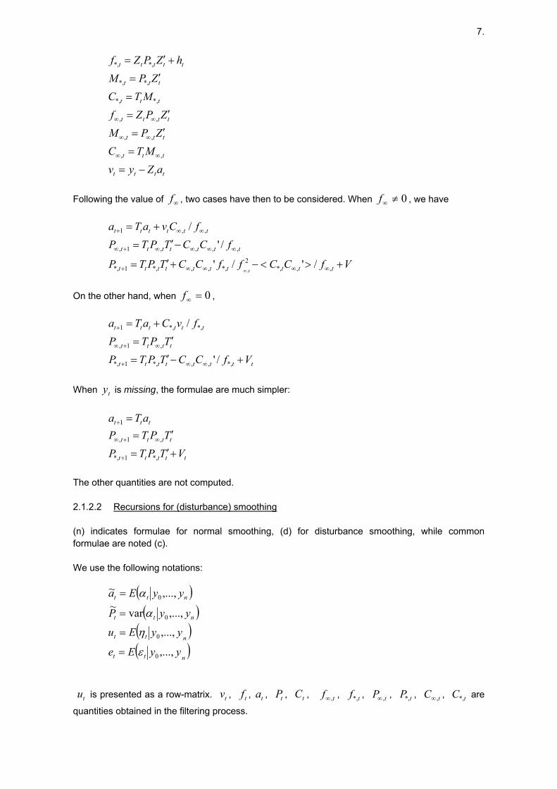
Diffuse recursions Diffuse recursion appends during the first periods; the length of the diffuse part is dynamically determined during the filtering process. When is not missing, a first set of formulae is defined by ty

3 is set to 1 (except for the likelihood evaluation). <A> stands for A+A'. 2σ

7.

tttt

ttt

ttt

tttt

ttt

ttt

ttttt

aZyvMTCZPMZPZf

MTCZPM

hZPZf

−=

=

′=

′=

=

′=

+′=

∞∞

∞∞

∞∞

,,

,,

,,

*,*,

*,*,

*,*,

Following the value of , two cases have then to be considered. When ∞f 0≠∞f , we have

VfCCffCCTPTP

fCCTPTPfCvaTa

tttttttttt

ttttttt

tttttt

t+><−+′=

−′=

+=

∞∞∞∞+

∞∞∞∞+∞

∞∞+

∞ ,,*,2

*,,,*,1*,

,,,,1,

,,1

/'/'

/'/

,

On the other hand, when , 0=∞f

tttttttt

tttt

tttttt

VfCCTPTPTPTP

fvCaTa

+−′=

′=

+=

∞∞+

∞+∞

+

*,,,*,1*,

,1,

*,*,1

/'

/

When is missing, the formulae are much simpler: ty

ttttt

tttt

ttt

VTPTPTPTP

aTa

+′=

′==

+

∞+∞

+

*,1*,

,1,

1

The other quantities are not computed. 2.1.2.2 Recursions for (disturbance) smoothing (n) indicates formulae for normal smoothing, (d) for disturbance smoothing, while common formulae are noted (c). We use the following notations:

( )( )

( )( )

ntt

ntt

ntt

ntt

yyEe

yyEu

yyP

yyEa

,...,

,...,

,...,var~,...,~

0

0

0

0

ε

η

α

α

=

=

=

=

tu is presented as a row-matrix. , , , , , , , , , , are

quantities obtained in the filtering process. tv tf ta tP tC tf , ∞ tf*, tP , ∞ tP*, tC , ∞ tC*,

8.

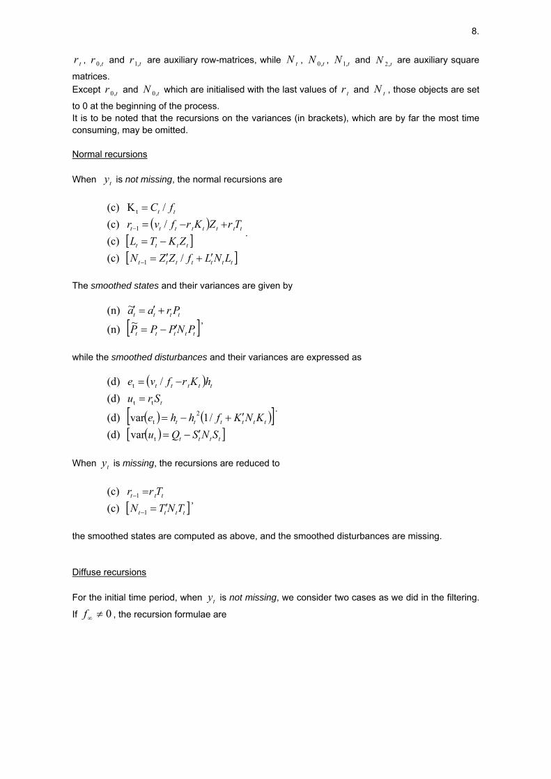
tr , and are auxiliary row-matrices, while , , and are auxiliary square

matrices. tr ,0 tr ,1 tN tN ,0 tN ,1 tN ,2

Except and which are initialised with the last values of and , those objects are set

to 0 at the beginning of the process. tr ,0 tN ,0 tr tN

It is to be noted that the recursions on the variances (in brackets), which are by far the most time consuming, may be omitted. Normal recursions When is not missing, the normal recursions are ty

( )[ ][ ]ttttttt

tttt

tttttttt

tt

LNLfZZNZKTL

TrZKrfvrfC

′+′=−=

+−==

−

−

/ (c) (c)

/ (c)/K (c)

1

1

t

.

The smoothed states and their variances are given by

[ ]ttttt

tttt

PNPPP

Praa′−=

+′=′~ (n)

~ (n),

while the smoothed disturbances and their variances are expressed as

( )

( ) ( )[ ]( )[ ]tttt

tttttt

t

ttttt

SNSQuKNKfhhe

SruhKrfve

′−=

′+−=

=−=

t

2t

tt

t

var (d)/1var (d)

(d)/ (d)

.

When is missing, the recursions are reduced to ty

[ ]tttt

ttt

TNTNTrr′=

=

−

−

1

1

(c) (c)

,

the smoothed states are computed as above, and the smoothed disturbances are missing.

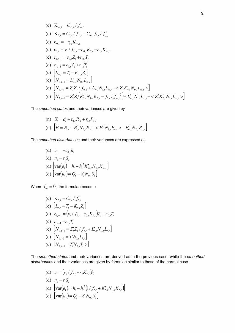
Diffuse recursions For the initial time period, when is not missing, we consider two cases as we did in the filtering.

If , the recursion formulae are ty

0≠∞f

9.

[ ][ ][ ]

( )[ ]>′′<−′+−′′=

>′′<−′+′=

′=

−=

+=

+=

−−=

−=

−=

=

∞∞∞∞−

∞∞∞∞−

∞∞−

∞∞

−

−

∞∞

∞

∞∞

∞∞∞

∞

ttttttttttttttt

ttttttttttt

tttt

tttt

ttttt

ttttt

tttttt

t

tttt

tt

LNKZLNLffKNKZZN

LNKZLNLfZZNLNLNZKTLTrZcrTrZcr

KrKrfvKr

ffCfC

fC

t

,,1*,,,1,2

,*,*,,0*,1,2

,,0*,,,1,,1,1

,,0,1,0

,,

,1,11,1

,0,01,0

,,1*,,0,t1,

t,,0t0,

2*,,,*,t,*

,,t,

/ (c)

/ (c) (c) (c) (c) (c)

/c (c)c (c)

//K (c)

/K (c)

,

The smoothed states and their variances are given by

[ ]ttttttttttt

tttttt

PNPPNPPNPPP

PrPraa

,,2,,,1*,*,*,*,*,

,,1*,,0~ (n)

~ (n)

∞∞∞

∞

′−>′<−′−=

++′=′

The smoothed disturbances and their variances are expressed as

( )[ ]( )[ ] var (d)

var (d)

(d) (d)

,0t

,,0,2

t

tt

,0t

tttt

ttttt

t

tt

SNSQuKNKhhe

Sruhce

′−=

′−=

=

−=

∞∞

When , the formulae become 0=∞f

[ ]( )

[ ][ ][ ]>′=

′=

′+′=

=

+−=

−=

=

−

−

−

−

−

tttt

tttt

ttttttt

ttt

tttttttt

tttt

tt

TNTNLNTN

LNLfZZNTrr

TrZKrfvrZKTL

fC

,21,2

*,,11,1

*,,0*,*,1,0

,11,1

,0*,,0*,1,0

*,*,

*,*,t,*

(c) (c)

/ (c) (c)

/ (c) (c)

/K (c)

The smoothed states and their variances are derived as in the previous case, while the smoothed disturbances and their variances are given by formulae similar to those of the normal case

( )

( ) ( )[ ]( )[ ]tttt

tttttt

t

ttttt

SNSQuKNKfhhe

SruhKrfve

,0t

*,,0*,*,2

t

tt

*,*,t

var (d)/1var (d)

(d)/ (d)

′−=

′+−=

=

−=

10.

When is missing, the recursions are reduced to ty

[ ][ ][ ]tttt

tttt

tttt

ttt

ttt

TNTNTNTNTNTN

TrrTrr

,21,2

,11,1

,01,0

,11,1

,01,0

(c) (c) (c) (c) (c)

′=

′=

′=

=

=

−

−

−

−

−

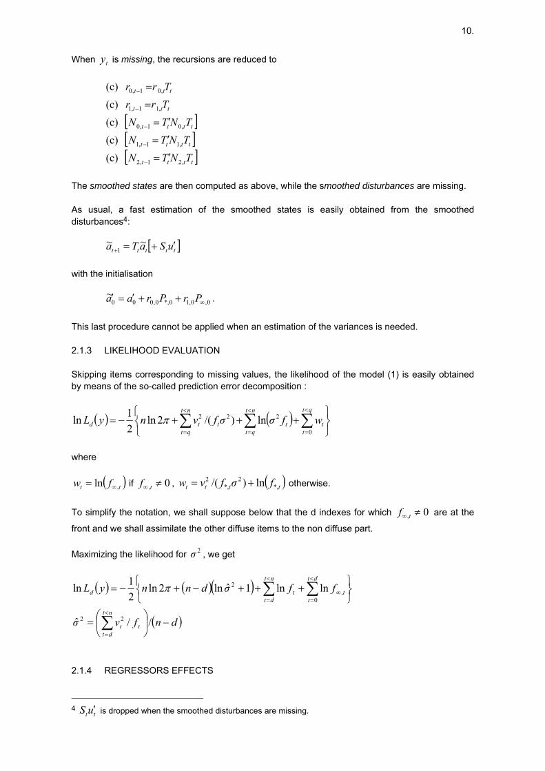
The smoothed states are then computed as above, while the smoothed disturbances are missing. As usual, a fast estimation of the smoothed states is easily obtained from the smoothed disturbances4:

[ ]ttttt uSaTa ′+=+~~

1

with the initialisation

0,0,10*,0,000~

∞++′=′ PrPraa .

This last procedure cannot be applied when an estimation of the variances is needed. 2.1.3 LIKELIHOOD EVALUATION Skipping items corresponding to missing values, the likelihood of the model (1) is easily obtained by means of the so-called prediction error decomposition :

( ) ( )⎭⎬⎫

⎩⎨⎧

+++−= ∑∑∑<

=

<

=

<

=

qt

tt

nt

qtt

nt

qtttd wfσσfvnyL

0

222 ln)/(2ln21ln π

where

( )tt fw ,ln ∞= if , 0, ≠∞ tf ( )tttt fσfvw *,2

*,2 ln)/( += otherwise.

To simplify the notation, we shall suppose below that the d indexes for which are at the

front and we shall assimilate the other diffuse items to the non diffuse part.

0, ≠∞ tf

Maximizing the likelihood for , we get 2σ

( ) ( )( )

( )dnfvσ

ffσdnnyL

nt

dttt

dt

tt

nt

dttd

−⎟⎠

⎞⎜⎝

⎛=

⎭⎬⎫

⎩⎨⎧

+++−+−=

∑

∑∑<

=

<

=∞

<

=

//ˆ

lnln1ˆln2ln21ln

22

0,

2π

2.1.4 REGRESSORS EFFECTS 4 is dropped when the smoothed disturbances are missing. ttuS ′

11.

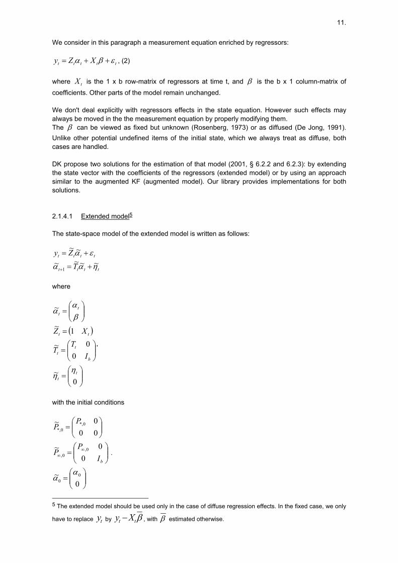
We consider in this paragraph a measurement equation enriched by regressors:

ttttt XZy εβα ++= , (2)

where is the 1 x b row-matrix of regressors at time t, and tX β is the b x 1 column-matrix of

coefficients. Other parts of the model remain unchanged. We don't deal explicitly with regressors effects in the state equation. However such effects may always be moved in the the measurement equation by properly modifying them. The β can be viewed as fixed but unknown (Rosenberg, 1973) or as diffused (De Jong, 1991). Unlike other potential undefined items of the initial state, which we always treat as diffuse, both cases are handled. DK propose two solutions for the estimation of that model (2001, § 6.2.2 and 6.2.3): by extending the state vector with the coefficients of the regressors (extended model) or by using an approach similar to the augmented KF (augmented model). Our library provides implementations for both solutions. 2.1.4.1 Extended model5 The state-space model of the extended model is written as follows:

tttt

tttt

T

Zy

ηαα

εα~~~~

~~

1 +=

+=

+

where

( )

⎟⎟⎠

⎞⎜⎜⎝

⎛=

⎟⎟⎠

⎞⎜⎜⎝

⎛=

=

⎟⎟⎠

⎞⎜⎜⎝

⎛=

0~

00~

1~

~

tt

b

tt

tt

tt

IT

T

XZ

ηη

βα

α

,

with the initial conditions

⎟⎟⎠

⎞⎜⎜⎝

⎛=

⎟⎟⎠

⎞⎜⎜⎝

⎛=

⎟⎟⎠

⎞⎜⎜⎝

⎛=

∞∞

0~

00~

000~

00

0,0,

0*,0*,

αα

bIP

P

PP

.

5 The extended model should be used only in the case of diffuse regression effects. In the fixed case, we only

have to replace by ty βtt Xy − , with β estimated otherwise.

12.

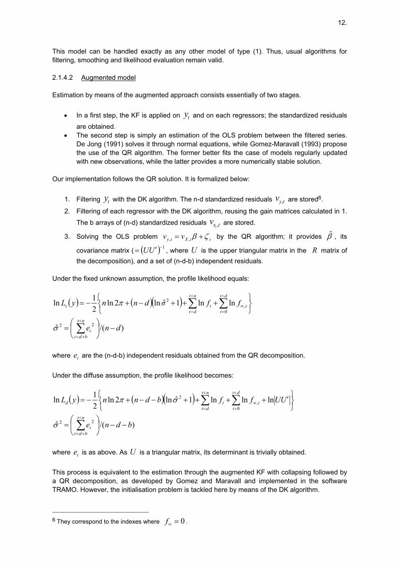
This model can be handled exactly as any other model of type (1). Thus, usual algorithms for filtering, smoothing and likelihood evaluation remain valid. 2.1.4.2 Augmented model Estimation by means of the augmented approach consists essentially of two stages.

• In a first step, the KF is applied on and on each regressors; the standardized residuals

are obtained. ty

• The second step is simply an estimation of the OLS problem between the filtered series. De Jong (1991) solves it through normal equations, while Gomez-Maravall (1993) propose the use of the QR algorithm. The former better fits the case of models regularly updated with new observations, while the latter provides a more numerically stable solution.

Our implementation follows the QR solution. It is formalized below:

1. Filtering with the DK algorithm. The n-d standardized residuals are storedty tyv ,6.

2. Filtering of each regressor with the DK algorithm, reusing the gain matrices calculated in 1.

The b arrays of (n-d) standardized residuals are stored. txiv ,

3. Solving the OLS problem ttXty vv ζβ += ,, by the QR algorithm; it provides , its

covariance matrix ( , where U is the upper triangular matrix in the

β̂

( ) 1−′= UU R matrix of the decomposition), and a set of (n-d-b) independent residuals.

Under the fixed unknown assumption, the profile likelihood equals:

( ) ( )( )

)/(ˆ

lnln1ˆln2ln21ln

22

0,

2

dne

ffσdnnyL

nt

bdtt

dt

tt

nt

dttc

−⎟⎠

⎞⎜⎝

⎛=

⎭⎬⎫

⎩⎨⎧

+++−+−=

∑

∑∑<

+=

<

=∞

<

=

σ

π

where are the (n-d-b) independent residuals obtained from the QR decomposition. te Under the diffuse assumption, the profile likelihood becomes:

( ) ( )( )

)/(ˆ

lnlnln1ˆln2ln21ln

22

0,

2

bdne

UUffbdnnyL

nt

bdtt

dt

tt

nt

dttd

−−⎟⎠

⎞⎜⎝

⎛=

⎭⎬⎫

⎩⎨⎧ ′++++−−+−=

∑

∑∑<

+=

<

=∞

<

=

σ

σπ

where is as above. As U is a triangular matrix, its determinant is trivially obtained. te This process is equivalent to the estimation through the augmented KF with collapsing followed by a QR decomposition, as developed by Gomez and Maravall and implemented in the software TRAMO. However, the initialisation problem is tackled here by means of the DK algorithm.

6 They correspond to the indexes where 0=∞f .

13.

The extended approach and the augmented approach yield the same likelihood evaluation. Both solution present some advantages. The former produces recursive residuals and recursive estimates of the coefficients. Recursive residuals are serially uncorrelated and easily interpretable, while recursive estimates are interesting for a study on the revisions. The latter is more stable and often faster. We use the extended model in the analysis stage while we prefer the augmented model during the optimization procedure.

2.2 BENCHMARKING

2.2.1 GENERALITIES The main goal of the present implementation of benchmarking is to provide a solution that encompasses popular techniques (Chow-Lin, Fernandez, Litterman, Denton, ...) Like Proietti (2004) we concentrate on single regression equations, with errors described by state-space forms. The library gives solutions for the distribution of a flux variable as well as for the interpolation of a stock variable. Estimation of the latter doesn't require special devices; it just amounts to the familiar problem of missing observations. We shall not consider it in details. The distribution case is handled through the use of cumulator variables (see Harvey, 1989, § 6.3). We shall also discuss the problem of log-transformed models, for which we provide approximated and iterative solutions. This last point is once again largely inspired by the work of Proietti (2004). 2.2.2 DISAGGREGATED TIME SERIES MODEL We suppose that the disaggregated time series admits a state space representation similar to (2). However, to simplify the derivation, we do not allow a disturbance term in the measurement equation7. In summary, the disaggregated model is

[ ]

tttt

ttt

ttt

TZ

Xy

ηαααµ

βµ

+==

+=

+1

with the other hypotheses as above. Apart from some assumptions on the initial values, the most popular disaggregation methods fit this form (see Proietti (2004) for a detailed discussion on that point); this is summarized in the following table: Methods Regressors Residuals ( tµ )

Chow-Lin constant + related series ARIMA(1, 0, 0) Litterman [linear trend +] related series ARIMA(1, 1, 0) Fernandez [linear trend +] related series ARIMA(0, 1, 0) Denton (K) ARIMA(0, K, 0)

7We can easily get around that condition by adding the disturbance term, if any, to the state vector.

14.

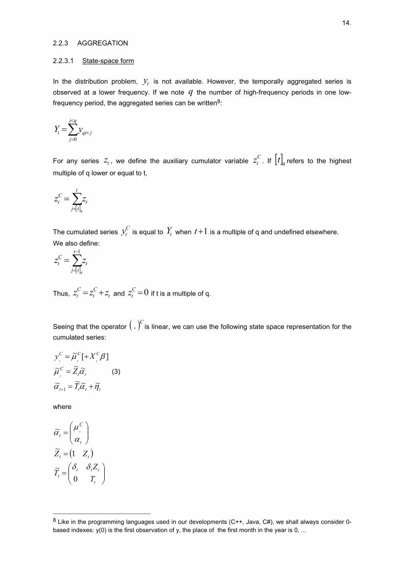
2.2.3 AGGREGATION 2.2.3.1 State-space form

In the distribution problem, is not available. However, the temporally aggregated series is observed at a lower frequency. If we note the number of high-frequency periods in one low-frequency period, the aggregated series can be written

tyq

8:

∑<

=+=

qj

jjqtt yY

0

For any series , we define the auxiliary cumulator variable . If tzCtz [ ]qt refers to the highest

multiple of q lower or equal to t,

[ ]∑=

=t

tjt

Ct

q

zz

The cumulated series is equal to when Cty tY 1+t is a multiple of q and undefined elsewhere.

We also define:

[ ]∑−

=

=1t

tjt

Ct

q

zz

Thus, tCt

Ct zzz += and 0=Ctz if t is a multiple of q.

Seeing that the operator is linear, we can use the following state space representation for the cumulated series:

( )C .

tttt

ttC

CCC

T

Z

Xy

t

ttt

ηαα

αµ

βµ

~~~~

~~~][~

1 +=

=

+=

+

(3)

where

( )

⎟⎟⎠

⎞⎜⎜⎝

⎛=

=

⎟⎟⎠

⎞⎜⎜⎝

⎛=

t

tttt

tt

t

C

t

TZ

T

ZZ

t

0~

1~

~

δδ

αµ

α

8 Like in the programming languages used in our developments (C++, Java, C#), we shall always consider 0-based indexes: y(0) is the first observation of y, the place of the first month in the year is 0, ...

15.

⎟⎟⎠

⎞⎜⎜⎝

⎛=

⎟⎟⎠

⎞⎜⎜⎝

⎛=

00

0~

0~

αα

ηη

tt

with 0=tδ if is a multiple of q, 1+t 1=tδ otherwise.

It is to be noted that the disaggregated series can be easily retrieved from the state vector of model

(3) by means of the matrix ; we have indeed ( tZZt

0=µ ) [ ]βαµ ttt XZyt

+= .

2.2.3.2 Estimation of the aggregated model The estimation of the aggregated model by itself is a straighforward application of the KF on the "cumulated" model (3).

As far as performances matter, the computing of the smoothed estimate )(~ nyEy tt = of the

disaggregated series requires some care. Depending on the presence of regressors and wether we need to obtain the variance of the smoothed series or not, we use the following schemes:

• No regressors, disaggregated series only

o Disturbance smoother on Cty

o tt tZy αµ

~~ =

• No regressors, disaggregated series and its variance

o Standard smoother on Cty

o tt tZy αµ

~~ =

o tt

ZZy tt µµ α ′= )~var()~var(

• Regressors, disaggregated series only

o Disturbance smoother on . β̂CCttXy −

o tt tZv αµ

~~ =

o β̂~~ttt Xvy +=

• Regressors, disaggregated series and its variance

o Standard smoother on . β̂CCttXy −

o tt tZv αµ

~~ =

o tt

ZZv tt µµ α ′= )~var()~var(

o Disturbance smoother on each cumulated regressor. tX~

are obtained

o β̂~~ttt Xvy +=

16.

o )~)(ˆvar()~()~var()~var( ′−−+= tttttt XXXXvy β

2.2.3.3 Logarithmic transformation Time series are often modelled in terms of the logarithms of their original data. As the logarithmic transformation is not additive, the distribution method exposed above can not be applied directly. We shall consider an approximated solution, which sum up to a small adaptation of the previous method (see Di Fonzo, 2003) and the Iterative method developped by Proietti (2004). The former will be our starting point for the latter. More formally, we consider in this paragraph that the state-space form is defined on the logarithmic transformation of the disaggregated series.

[ ]

tttt

ttt

tttt

TZ

Xzy

ηαααµ

βµ

+==

+==

+1

ln(4)

The aggregation constraint is now non linear. The different options implemented in the library are detailed below. 2.2.3.3.1 Approximated solution By using the Taylor series expansion of around the average of during each aggregated

period, it can be easily seen that tyln ty

∑≈− qt yqqYq lnlnln

The logarithmic model can thus be approximated by the linear solution, if we properly transform the aggregated values. As suggested in Di Fonzo (2003), we shall restore the exact aggregation constraints by distributing the residuals with the Denton's method. 2.2.3.3.2 Iterative solution Using a reasoning similar to the Proietti's one (2004), given a trial disaggregated series

)~exp(~tt zy = , the Taylor expansion of )exp( tt zy = around tz~ yields:

ttttt zzzzy )~exp()~1)(~exp( +−≈

Applying the cumulator operator, we get:

]))~(exp([))~(exp())~1)(~(exp( βµ Ctt

Ctt

Ctt

C Xzzzzyt

+=−−

If we pose

17.

( ))~exp(

)~1)(~exp(

tt

Ctt

Ct

zs

zzyKt

=

−−=

the previous equation can be more concisely expressed as

( ) ( ) ][ βµ Ctt

Cttt XssK +=

The state-space form of the linear gaussian approximated model (LGAM) conditional to tz~ is then

formulated as follows:

tttt

ttC

tt

T

Zs

ηαα

αµ~~~~

~~)~(

1 +=

=

+

(5)

with

( )

( )

⎟⎟⎠

⎞⎜⎜⎝

⎛=

⎟⎟⎠

⎞⎜⎜⎝

⎛=

⎟⎟⎠

⎞⎜⎜⎝

⎛=

=

⎟⎟⎠

⎞⎜⎜⎝

⎛=

00

0~

0~

0~

1~

~

αα

ηη

δδ

αµα

tt

t

ttttt

ttt

t

Ctt

t

TZs

T

ZsZ

s

Applying the KF and the disturbance smoother (see 4.4), a new estimate of the disaggregated series is computed. The process is iterated until convergence. As starting values, we take the solution of the approximated solution (without the final Denton correction) as defined in 2.2.3.3.1. The likelihood of the model is approximated by that of the LGAM at convergence. It should be noted that the iterative process doesn't necessarily converge. This is more often the case when the starting values are far from their optimum. If some parameters of the model have to be estimated by ML, a good solution seems to start the maximization procedure from the ML estimates of the approximated logarithmic model. Our implementation works in that way. 2.2.4 PRACTICAL CONSIDERATIONS Aggregation leads to a substantial loss of information. In practice, only very parsimonious models can be estimated in a relatively stable way. Moreover, many SSF, for example those including seasonal unit roots, lead to degenerate aggregation models. Even if the library allows the use of complex SSF for the residuals, those simple observations justify why we shall restrict our applications, in many cases, to a small subset of models, including the most traditional solutions. It should also be noted that, as far as ARIMA residuals are considered, models for distribution can be easily transformed to models for interpolation9: seeing that stocks are simply an accumulation of flux, we can move from one case to the other by accumulating the aggregated series and the

9 This is not true when we are dealing with log-transformed models.

18.

related series (the starting values don't matter) and by adding a unit root to the model of the residuals. The versatility of the library allows the statistical treatment and comparison of both solutions. This is also a way to verify some results with other software (for instance TRAMO).

3 OO-DESIGN

The object-oriented paradigm offers well-known facilities to achieve extensibility. We shall show in the next paragraphs how they are exploited in our library leading to efficient and flexible implementations of KF.

3.1 STATE SPACE MODELS

3.1.1 GENERAL CONSIDERATIONS While general forms of KF, based on matrix computation, can be quite easily developed, faster implementations must exploit the structure of the matrices involved in the KF. Those structures are specific to each kind of model. By exploiting them, we can achieve a substantial gain in performances. The OO-design of the library is based on those considerations. Common features, like the whole logic in the filtering, smoothing, likelihood evaluation, ... will be handled by general entities while the actual computation will be delegated to implementations of specific models. We shall clarify that point by an example. The filtering process involves several operations that multiply an array by the transformation matrix

(see 2.1.2, , tT ttttt fZPTK /′= ttttt vKaTa +=+1 ).

Instead of using actual matrix computations, we shall impose on each specific SSF to provide a function that performs that multiplication ( ),( xtfxTy Txt == ). In many cases, that function will be

simple and much faster than matrix computation. For example, in the case of an ARIMA model (see appendix 1 for its SSF), the operation

is defined by ),( xtfy Tx=

∑=

−−=−

<<=−P

iirxiry

riixiy

1)()()1(

0),()1(

φ

where the )(iφ are the P coefficients of the autoregressive polynomial. It involves P (<=r) multiplications while the blind matrix computation needs 2r multiplications and more memory traffic. A similar reasoning could be applied to other operations like, for example,

(multiplication by the measurement matrix), or like

),( xtfxZ Zxt =),( xtfxT xTt = (right-multiplication by the

transition matrix, used in the smoothing process). Thus, besides the description of the different matrices listed in § 2.1.1, the definition of a generic SSF (see appendix 2) also precise some "basic operations" for a faster processing. The common algorithms only call generic properties and methods; so they remain valid for any (new)

19.

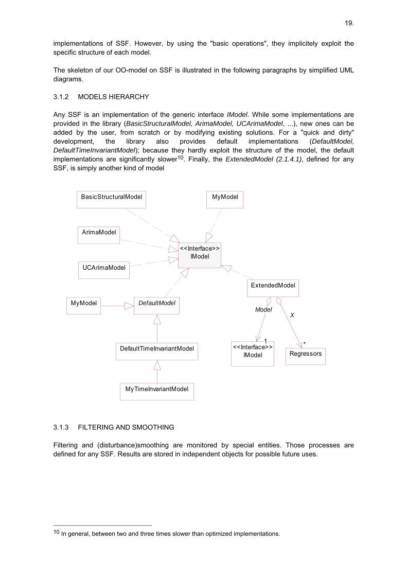
implementations of SSF. However, by using the "basic operations", they implicitely exploit the specific structure of each model. The skeleton of our OO-model on SSF is illustrated in the following paragraphs by simplified UML diagrams. 3.1.2 MODELS HIERARCHY Any SSF is an implementation of the generic interface IModel. While some implementations are provided in the library (BasicStructuralModel, ArimaModel, UCArimaModel, ...), new ones can be added by the user, from scratch or by modifying existing solutions. For a "quick and dirty" development, the library also provides default implementations (DefaultModel, DefaultTimeInvariantModel); because they hardly exploit the structure of the model, the default implementations are significantly slower10. Finally, the ExtendedModel (2.1.4.1), defined for any SSF, is simply another kind of model

MyModel DefaultModel

IModel<<Interface>>

ArimaModel

UCArimaModel

BasicStructuralModel

DefaultTimeInvariantModel

MyTimeInvariantModel

MyModel

IModel<<Interface>>

ExtendedModel

11

Model

Regressors**

X

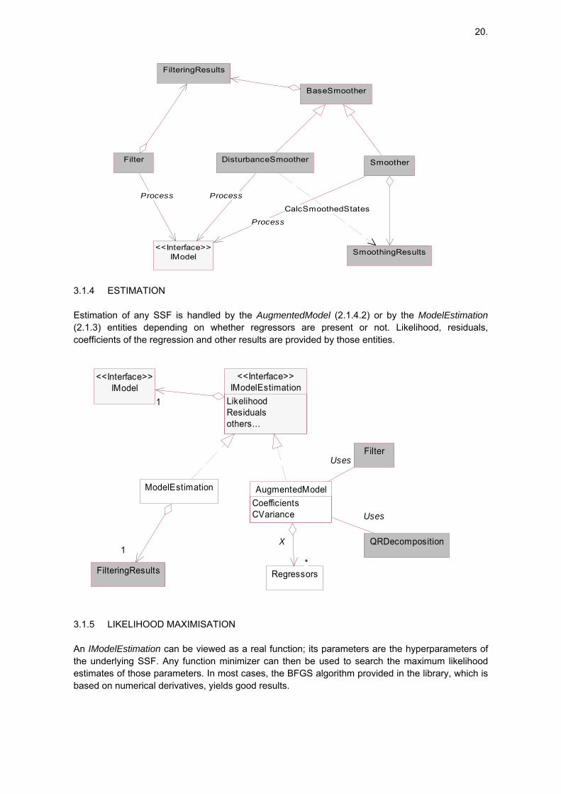
3.1.3 FILTERING AND SMOOTHING Filtering and (disturbance)smoothing are monitored by special entities. Those processes are defined for any SSF. Results are stored in independent objects for possible future uses.

10 In general, between two and three times slower than optimized implementations.

20.

SmoothingResults

DisturbanceSmoother

IModel<<Interface>>

Process

Smoother

Process

Filter

Process

BaseSmoother

FilteringResults

CalcSmoothedStates

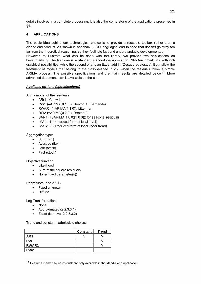
3.1.4 ESTIMATION Estimation of any SSF is handled by the AugmentedModel (2.1.4.2) or by the ModelEstimation (2.1.3) entities depending on whether regressors are present or not. Likelihood, residuals, coefficients of the regression and other results are provided by those entities.

IModel<<Interface>>

IModelEstimationLikelihoodResidualsothers...

<<Interface>>

11

Regressors

QRDecomposition

FilteringResults

ModelEstimation

11

AugmentedModelCoefficientsCVariance

**

X

Uses

FilterUses

3.1.5 LIKELIHOOD MAXIMISATION An IModelEstimation can be viewed as a real function; its parameters are the hyperparameters of the underlying SSF. Any function minimizer can then be used to search the maximum likelihood estimates of those parameters. In most cases, the BFGS algorithm provided in the library, which is based on numerical derivatives, yields good results.

21.

MyMinimizer

IParametriseable<<Interface>>

Marquardt

IRealFunction<<Interface>>

IFunctionMinimizer<<Interface>>

Minimize

NumericalDerivatives

BFGS

Uses

IModel<<Interface>>

IModelEstimation<<Interface>>

11

3.2 BENCHMARKING

Apart from some small details, our implementation of benchmarking is a straighforward application of the KF algorithms of § 2.1, with the different SSF defined in § 2.2. The library provides three kinds of benchmarking models. The first one, GenericExpander, is an exact translation of the model (3): it accepts residuals represented by any SSF, provided that its measurement equation doesn't contain disturbances. ArimaExpander objects are entities specialized for the handling of benchmarking models with ARIMA residuals; the most popular solutions belong to that case. Finally, the LogArimaExpander class modifies the previous one to deal with the state-space form (5), used in the iterative approach of the log-transformed model.

Result

IModel<<Interface>> GenericExpander

IModel<<Interface>>11

IModelEstimation<<Interface>>

IArimaModel<<Interface>>

TsRegressors

Ts

Ts

ArimaExpander

11

Ts

LogArimaExpander

TsArimaExpander

Estimation

ArimaModel

Regressors

Process

Uses

11

OnePeriodAheadResiduals

Uses

Model 2.2.3.1, with ARIMA errors

Model 2.2.3.3.2,with ARIMA errors

Model 2.2.3.1. General

The high-level entity TsArimaExpander allows an easier treatment of the different solutions in the case of SSF with ARIMA residuals. It also provides many auxiliary results and hides most of the

22.

details involved in a complete processing. It is also the cornerstone of the applications presented in §4.

4 APPLICATIONS

The basic idea behind our technological choice is to provide a reusable toolbox rather than a closed end product. As shown in appendix 3, OO languages lead to code that doesn't go stray too far from the theoretical reasoning; so they facilitate fast and understandable developments . However, to illustrate what can be done with the library, we provide two applications on benchmarking. The first one is a standard stand-alone application (NbbBenchmarking), with rich graphical possibilities, while the second one is an Excel add-in (Desaggregator.xls). Both allow the treatment of models that belong to the class defined in 2.2, when the residuals follow a simple ARIMA process. The possible specifications and the main results are detailed below11. More advanced documentation is available on the site. Available options (specifications) Arima model of the residuals

• AR(1): Chow-Lin • RW1 (=ARIMA(0 1 0)): Denton(1), Fernandez • RWAR1 (=ARIMA(1 1 0)): Litterman • RW2 (=ARIMA(0 2 0)): Denton(2) • SAR1 (=SARIMA(1 0 0)(1 0 0)): for seasonal residuals • IMA(1, 1) (=reduced form of local level) • IMA(2, 2) (=reduced form of local linear trend)

Aggregation type:

• Sum (flux) • Average (flux) • Last (stock) • First (stock)

Objective function

• Likelihood • Sum of the square residuals • None (fixed parameter(s))

Regressors (see 2.1.4)

• Fixed unknown • Diffuse

Log Transformation

• None • Approximated (2.2.3.3.1) • Exact (iterative, 2.2.3.3.2)

Trend and constant : admissible choices: Constant Trend AR1 V V RW V RWAR1 V RW2

11 Features marked by an asterisk are only available in the stand-alone application.

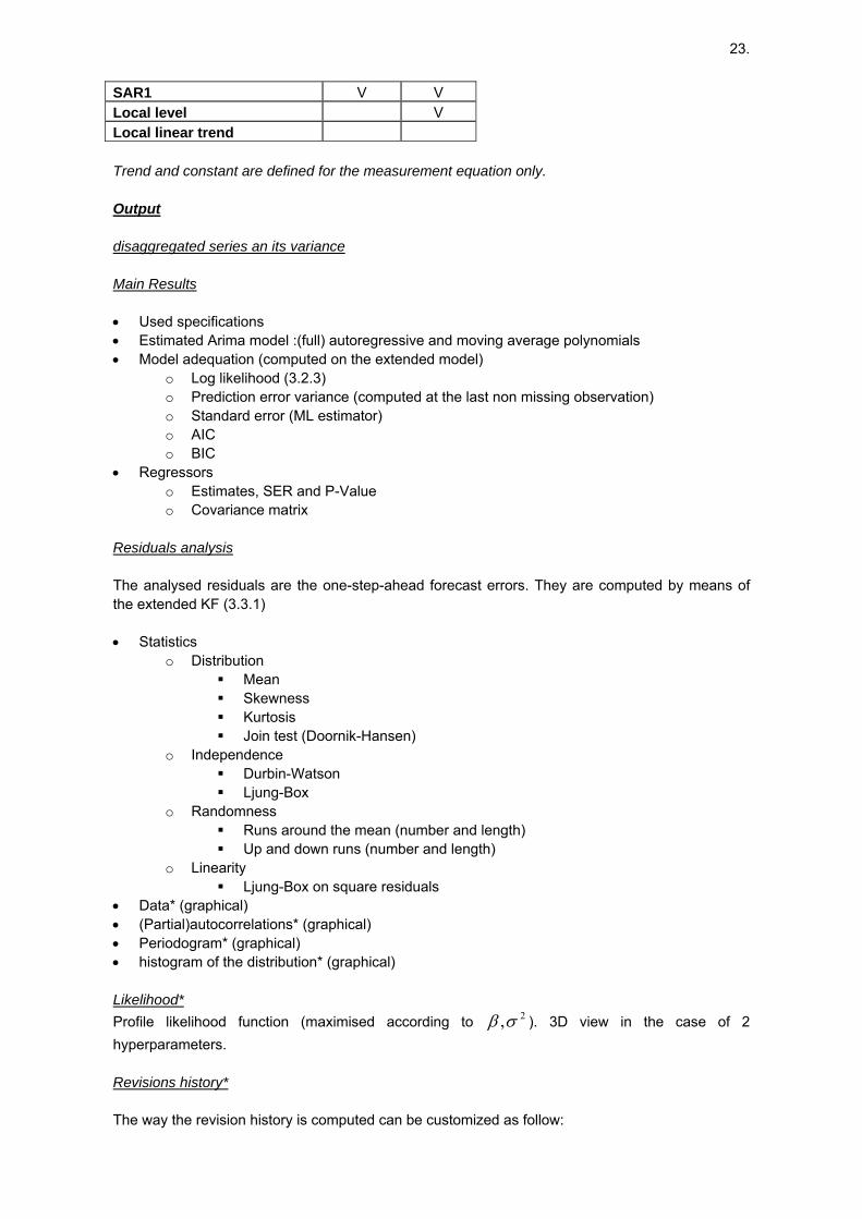
23.

SAR1 V V Local level V Local linear trend Trend and constant are defined for the measurement equation only. Output disaggregated series an its variance Main Results • Used specifications • Estimated Arima model :(full) autoregressive and moving average polynomials • Model adequation (computed on the extended model)

o Log likelihood (3.2.3) o Prediction error variance (computed at the last non missing observation) o Standard error (ML estimator) o AIC o BIC

• Regressors o Estimates, SER and P-Value o Covariance matrix

Residuals analysis The analysed residuals are the one-step-ahead forecast errors. They are computed by means of the extended KF (3.3.1) • Statistics

o Distribution Mean Skewness Kurtosis Join test (Doornik-Hansen)

o Independence Durbin-Watson Ljung-Box

o Randomness Runs around the mean (number and length) Up and down runs (number and length)

o Linearity Ljung-Box on square residuals

• Data* (graphical) • (Partial)autocorrelations* (graphical) • Periodogram* (graphical) • histogram of the distribution* (graphical) Likelihood* Profile likelihood function (maximised according to ). 3D view in the case of 2 hyperparameters.

2,σβ

Revisions history* The way the revision history is computed can be customized as follow:

24.

• The hyperparameters can be fixed or not (in the former case, the parameters computed on the

full period are kept, but the other quantities are re-estimated, while in the latter case, the full process is reexecuted on different time horizons).

• The number of re-estimations (with a minimun of observations) involved in the study may be defined.

The results are (if q is the number of high-frequency periods in one low-frequency period): • Errors

we consider the absolute differences between the final estimated values (on the whole period) and the results obtained on shorter periods. The errors are computed on the last q periods of the estimation and on the first q forecasting periods.

o mean of the errors o mean of the percentage errors o root mean square errors

The other results come from the estimation of the SSF on shortened periods.

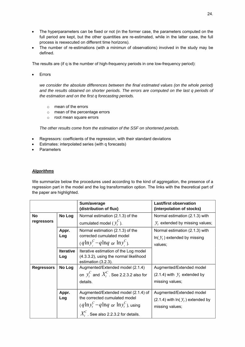
• Regressors: coefficients of the regression, with their standard deviations • Estimates: interpolated series (with q forecasts) • Parameters Algorithms We summarize below the procedures used according to the kind of aggregation, the presence of a regression part in the model and the log transformation option. The links with the theoretical part of the paper are highlighted. Sum/average

(distribution of flux) Last/first observation (interpolation of stocks)

No Log Normal estimation (2.1.3) of the

cumulated model ( ). Cty

Normal estimation (2.1.3) with

extended by missing values; tyAppr. Log

Normal estimation (2.1.3) of the corrected cumulated model

( or ). qqyq Ct

lnln − Ctyln

No regressors

IterativeLog

Iterative estimation of the Log model (4.3.3.2), using the normal likelihood estimation (3.2.3).

Normal estimation (2.1.3) with

ln( ) extended by missing

values; ty

No Log Augmented/Extended model (2.1.4)

on and . See 2.2.3.2 also for

details.

Cty

CtX

Augmented/Extended model

(2.1.4) with extended by

missing values; ty

Regressors

Appr. Log

Augmented/Extended model (2.1.4) of the corrected cumulated model

( or ), using

. See also 2.2.3.2 for details.

qqyq Ct lnln − C

tylnCtX

Augmented/Extended model

(2.1.4) with ln( ) extended by

missing values; ty

25.

IterativeLog

Augmented/Extended model (2.1.4) of the LGAM (2.2.3.3.2, iterative solution). See also 2.2.3.2 for other details.

Maximum likelihood estimates are computed through the BFGS procedure integrated in the library. They depend on the assumption made on the diffuse/non diffuse character of the regression effects.

5 FUTURE EXTENSIONS

It should be stressed that the solutions for benchmarking proposed in the present library are just simple applications of the whole underlying SSF framework. Starting from the current situation, other approaches could be quickly implemented (for example the model of Durbin and Quenneville, 1997). However, the main challenge is now to enrich the framework for handling multivariate models; so, the scope of application will be enlarged to other appealing solutions like common components models. By using the univariate treatment of multivariate series as described in DK (2001, § 6.4), that could be done in a reasonable delay (2006).

6 CONCLUDING REMARKS

The libraries developed by the R&D cell of the statistical department of the National Bank of Belgium are an attempt to combine recent developments around the SSF and new technologies. They are still in a prototyping phase; so, their algorithms and their results should be handled with some caution. Updates of the software and of the documentation will be regularly made available on the site of the Bank. Anyway, the present work already shows that the OO paradigm fits very well the versatility of the state-space models and that, through a good design, it is possible to achieve fast processing as well as flexibility. Reusability is also achieved by the use of standard technologies like Java and .NET. As far as benchmarking is concerned, state-space techniques provide a coherent framework for the traditional methods. Thanks to their high performances, they make feasible a variety of analysis devices. Finally, further improvements in the benchmarking domain should be obtained by means of a multivariate approach. External help, on the theoretical or methodological level, would be welcome.

26.

Bibliography De Jong P. (1989), "Smoothing and Interpolation With the State-Space Model", Journal of the American Statistical Association, 84, 408, 1085-1088. De Jong P. (1991), "Stable Algorithms For the State Space Model", Journal of Time Series Analysis, 12, 2, 143-157. De Jong P. and Chu-Chun-Lin S. (1994), "Fast likelihood evaluation and prediction for nonstationary State Space Models", Biometrika, 81, 1, 133-142. De Jong P. and Chu-Chun-Lin S. (2003), "Smoothing with an Unknown Initial Condition", Journal of Time Series Analysis, 24, 2, 141-148. Di Fonzo, T. (2003), "Temporal disaggregation of economic time series: towards a dynamic extension", working papers and studies, European Communities. Durbin J. and Koopman S.J. (2001), "Time Series Analysis by State Space Methods". Oxford University Press. Durbin J. and Koopman S.J. (2002), "A simple and efficient simulation smoother for state space time series analysis ", Biometrika, 89, 3, 603 - 615. Durbin J. and Koopman S.J. (2003), "Filtering and smoothing of state vector for diffuse state space models", Journal of Time Series Analysis, vol 24, n°1, 85 - 98. Durbin J. and Quenneville B. (1997), "Benchmarking by State Space Models", International Statistical Revieuw, vol 65, n°1, 23-48. Gomez V. and Maravall A. (1993), "Initializing the Kalman Filter with Incompletely Specified Initial Conditions", Working paper 93/7, European University Institute. Gomez V. and Maravall A. (1994), "Estimation, Prediction, and Interpolation for Nonstationary Seires With the Kalman Filter", Journal of the American Statistical Association, vol 89, n° 426, 611-624. Harvey, A.C. (1989), "Forecasting, Structural Time Series Models and the Kalman Filter", Cambridge University Press. Kohn R. and Ansley C.F. (1985), "Efficient estimation and prediction in time series regression models", Biometrika, 72, 3, 694-697. Koopman S.J. (1993). "Disturbance smoother for state space models", Biometrika, 80, 1, 117-126. Koopman S.J. and Harvey A. (1999), "Computing Observation Weights for Signal Extraction and Filtering". Proeitti T. (2004), "Temporal disaggregation by State Space Methods: Dynamic Regression Methods Revisited", working papers and studies, European Communities. Rosenberg, B. (1973), "Random coefficients models: the analysis of a cross-section of tile series by stochastically convergent parameter regression", Annals of Economic and Social Measurement, 2, 399-428.

27.

Appendix 1. State-space representation of an ARIMA model. The ARIMA process is defined by

( ) ( ) ( ) ( ) )(tBtyBB εΘ=Γ∆ , where

( )( )( ) q

q1

pp1

dd1

Bθ...Bθ1BΘ

B...B1B

Bδ...Bδ1B∆

+++=

+++=Γ

+++=

ϕϕ

are the differencing, auto-regressive and moving average polynomials. We also write:

( ) ( ) ( ) dpp1 B...B1BB∆BΦ ++++=Γ•= φφ

Let be the psi-weights of the Arima model, and iψ ist ,ψ ist ,γ , the psi-weights and the

autocovariances of the differenced Arma model. We also define:

( )1

1,max−=

++=rs

qdpr

Using those notations, the state-space model can be written as follows12: State vector:

⎟⎟⎟⎟⎟

⎠

⎞

⎜⎜⎜⎜⎜

⎝

⎛

+

+=

)(

)1()(

)(α

tsty

ttyty

tL

where )( tity + is the orthogonal projection of ( )ity + on the subspace generated by

. Thus, it is the forecast function with respect to the semi-infinite sample. { tssy ≤:)( } System matrices: Using the notations of § 3.1, the matrices of the model are

( ) ( )001 L=tZ

( ) 0=th

⎟⎟⎟⎟⎟⎟

⎠

⎞

⎜⎜⎜⎜⎜⎜

⎝

⎛

−−

=

1

1000

01000010

)(

φφ LLL

L

MOMMM

L

L

r

tT

12 See for example Gomez-Maravall (1994)

28.

( )

⎟⎟⎟⎟⎟⎟

⎠

⎞

⎜⎜⎜⎜⎜⎜

⎝

⎛

=

s

tW

ψ

ψψ

1

0

M

M

rItR =)(

2σ)( =tQ

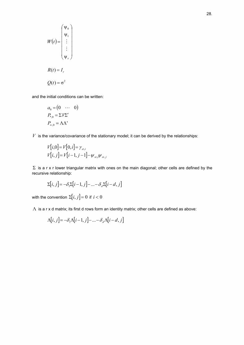
and the initial conditions can be written:

( )

'

00

0,

0*,

0

ΛΛ=

Σ′Σ==

∞PVP

a L

V is the variance/covariance of the stationary model; it can be derived by the relationships:

[ ] [ ][ ] [ ] jstist

ist

jiVjiViViV

,,

,

1,1,,00,

ψψγ

−−−=

==

Σ is a r x r lower triangular matrix with ones on the main diagonal; other cells are defined by the recursive relationship:

[ ] [ ] [ ]jdijiji d ,...,1, 1 −Σ−−−Σ−=Σ δδ

with the convention [ ] 0, =Σ ji if 0<i Λ is a r x d matrix; its first d rows form an identity matrix; other cells are defined as above:

[ ] [ ] [ ]jdijiji d ,...,1, 1 −Λ−−−Λ−=Λ δδ

29.

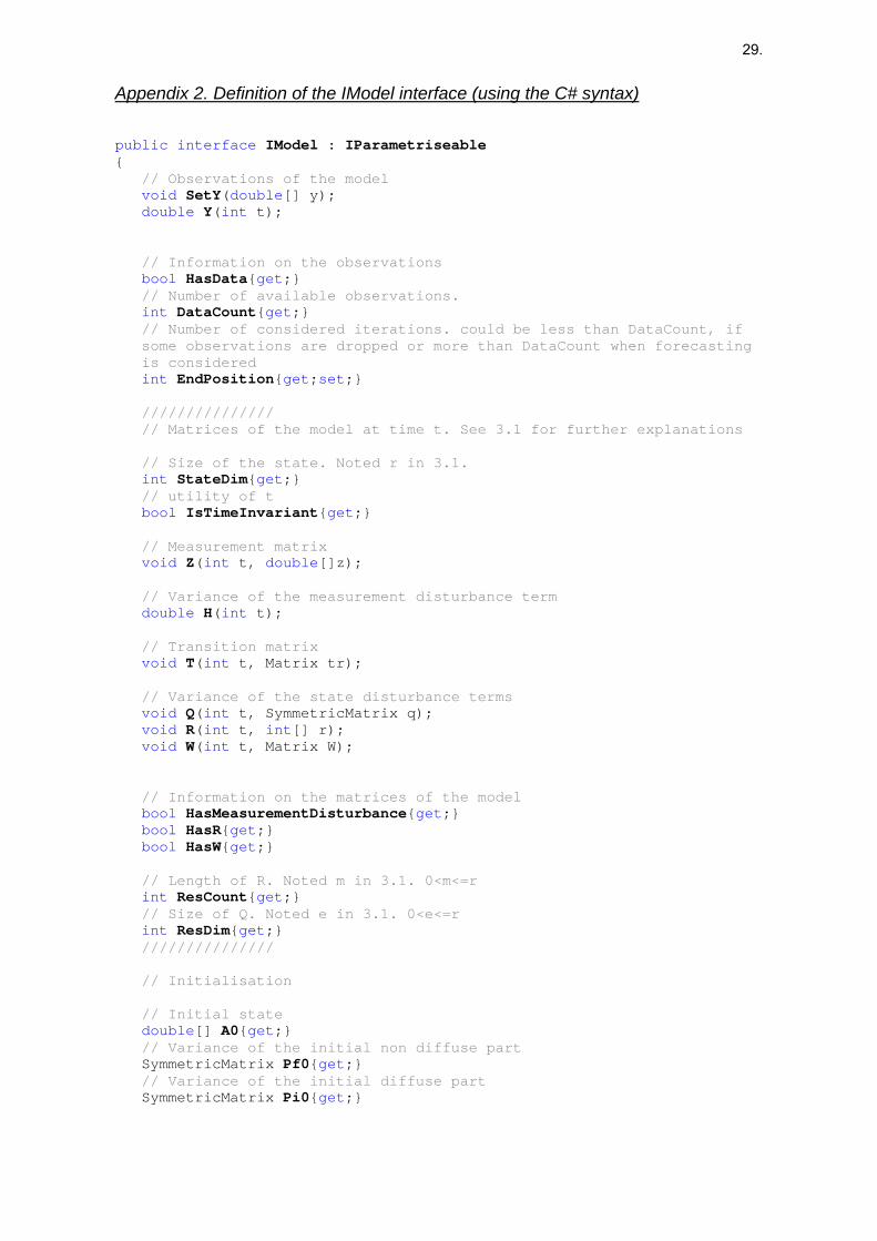
Appendix 2. Definition of the IModel interface (using the C# syntax) public interface IModel : IParametriseable {

// Observations of the model void SetY(double[] y); double Y(int t); // Information on the observations bool HasData{get;} // Number of available observations. int DataCount{get;} // Number of considered iterations. could be less than DataCount, if some observations are dropped or more than DataCount when forecasting is considered int EndPosition{get;set;} /////////////// // Matrices of the model at time t. See 3.1 for further explanations // Size of the state. Noted r in 3.1. int StateDim{get;} // utility of t bool IsTimeInvariant{get;} // Measurement matrix void Z(int t, double[]z); // Variance of the measurement disturbance term double H(int t); // Transition matrix void T(int t, Matrix tr); // Variance of the state disturbance terms void Q(int t, SymmetricMatrix q); void R(int t, int[] r); void W(int t, Matrix W); // Information on the matrices of the model bool HasMeasurementDisturbance{get;} bool HasR{get;} bool HasW{get;} // Length of R. Noted m in 3.1. 0<m<=r int ResCount{get;} // Size of Q. Noted e in 3.1. 0<e<=r int ResDim{get;} /////////////// // Initialisation // Initial state double[] A0{get;} // Variance of the initial non diffuse part SymmetricMatrix Pf0{get;} // Variance of the initial diffuse part SymmetricMatrix Pi0{get;}

30.

// Number of independent non-stationary components. equals rank of Pi0. Noted d in 3.1 int NonStationaryDim{get;} // d > 0 bool IsDiffuse{get;} /////////////// // Others informations bool IsValid{get;} // L = T - K*Z, K column-vector void L(int t, double[] K, Matrix l); /////////////// // Atomic operations // Forwards operations // xout = T*xin, xin column-vector void TX(int t, double[] xin, double[] xout); // Z*xin, xin column-vector double ZX(int t, double[] xin); // xout = Z*M, M matrix void ZM(int t, AbstractMatrix M, double[] xout); // V = T*V*T', the most time-consuming operation. It should be carefully optimized. void TVT(int t, SymmetricMatrix V); // Z*V*Z' double ZVZ(int t, SymmetricMatrix V); // Backwards operations // xout = xin*T, xin row-vector void XT(int t, double[] xin, double[] xout); // V = V + Z'*d*Z void VpZdZ(int t, SymmetricMatrix V, double d); // X = X + Z * d, X row-vector void XpZd(int t, double[] X, double d);

}

31.

Appendix 3. Examples of code (C# syntax). The goal of the following examples is just to give a fast overview of the capabilities of the library and of its conciseness. Real code needs of course much further documentation. /////////////////////////////////////////////////////////////////////// // Example 1. Computation of the likelihood of a Chow-Lin/Litterman model // following several ways. Quarterly series. Fixed parameter (-.9). /////////////////////////////////////////////////////////////////////// // Construction of an (RW)AR1 ARIMA model int freq=4; SArimaSpecification spec=new SArimaSpecification(freq); spec.P=1; // spec.D=1; // for litterman SArimaModel arima=new SArimaModel(spec); arima.Parameters=new double[]{-.9}; // double[] yc=... // double[][] x=..., xc=... // We suppose that yc, x, xc are respectively the aggregated series //(expanded with missing values), the related series and the cumulated // related series. // Contruction of a (Durbin-Koopman) SSF for the given ARIMA model // (see 2.1.1 and appendix 1) ArimaDKModel mSSF=new ArimaDKModel(arima); // Construction of an optimized benchmarking model for the given ARIMA // model (see 2.2.2) ArimaExpander mxSSF=new ArimaExpander(arima, freq); mxSSF.SetY(yc); // Augmented model (see 2.1.4.2) AugmentedModel agModel=new AugmentedModel(); agModel.Model= mxSSF; agModel.Regressors=xc; agModel.UseDiffuseRegressors(true); double agLL= agModel.LogLikelihood; // Extended model (see 2.1.4.1). Construction + Estimation ExtendedModel exSSF=new ExtendedModel(mxSSF, xc); ModelEstimation mEst=new ModelEstimation(); mEst.Model=exSSF; double exLL=mEst.LogLikelihood; // use of not optimized methods // Generic expansion (see 2.2.3.1) followed by Extended model GenericExpander gxSSF=new GenericExpander(mSSF,freq); ExtendedModel exg=new ExtendedModel(gxSSF, xc); exg.SetY(yc); mEst.Model=exg; double exgLL=mEst.LogLikelihood; // Extended model followed by Generic expansion ExtendedModel exm=new ExtendedModel(mSSF, x); GenericExpander gex=new GenericExpander(exm, freq); gex.SetY(yc); mEst.Model=gex; double gexLL=mEst.LogLikelihood; // It is to be noted that the previous two solutions imply quite

32.

// different SSF. Following the length and the frequency of the series, the performances of the previous solutions differ sometimes substantially. The table below gives the number of function evaluations per second. (Context: C# implementation, Windows XP, 3 Ghz CPU, 512 MB RAM). Chow-Lin Litterman Quarterly series

(15 years) Monthly series (15 years)

Quarterly series (15 years)

Monthly series (15 years)

Augmented model 4500 2050 3600 1750 Extended model 5600 2100 3400 1550 Generic expansion + extended model

3900 1450 2100 1000

Extended model + generic expansion

3300 1150 1900 600

/////////////////////////////////////////////////////////////////////// // Example 2. Benchmarking for a local linear trend. No regressors. // Estimation and smoothing. /////////////////////////////////////////////////////////////////////// // Construction of the basic structural model BSMSpecification bspec=new BSMSpecification(); bspec.HasSeas=false; bspec.HasSlope=true; BasicStructuralModel bsmSSF=new BasicStructuralModel(bspec, null, freq); bsmSSF.IsNoiseInState=true; // Generic expander. GenericExpander bsmxSSF=new GenericExpander(bsmSSF,freq); bsmxSSF.SetY(yc); // Likelihood function (see 2.1.3) ModelEstimation bsmEst=new ModelEstimation(); bsmEst.Model=bsmxSSF; // Optimization through BFGS. BFGS needs an auxiliary object to check the // validity of the parameters BFGS bfgs=new BFGS(); BSMChecker checker=new BSMChecker(); checker.UseParamsTransformation=false; if (bfgs.Minimize(bsmEst, checker)){ bsmEst=(ModelEstimation) bfgs.Result; bsmxSSF=(GenericExpander)bsmEst.Model; } // Smoothing of the generic expander SmoothingResults srslts=new SmoothingResults(); Smoother smoother=new Smoother(); smoother.Process(bsmxSSF, srslts); // the results can be further used. For example, the following code // yields the smoothed series (ys). double[] zorig=new double[bsmxSSF.StateDim]; double[] ys=new double[yc.Length]; for (int i=0; i<ys.Length; ++i){ bsmxSSF.ZOriginal(i, zorig); ys[i]=srslts.ZComponent(zorig); }