EPA/#June 2000

Workshop on UNMIX and PMFAs Applied to PM2.5

14-16 February 2000U.S. EPA, RTP, NC

Final Report

by

Robert D. WillisManTech Environmental Technology, Inc.

Research Triangle Park, NC 27709

Contract No. 68-D5-0049

Project OfficerPortia Britt

Work Assignment ManagerCharles W. Lewis

National Exposure Research LaboratoryHuman Exposure and Atmospheric Sciences Division

National Exposure Research LaboratoryOffice of Research and DevelopmentU.S. Environmental Protection Agency

Research Triangle Park, NC 27711

ii

Notice

The U.S. Environmental Protection Agency through its Office of Research and Development funded andmanaged the research described here under Contract 68-D5-0049 to ManTech Environmental Technology, Inc.It has been subjected to the Agency’s peer and administrative review and has been approved for publicationas an EPA document.

iii

Contents

Volume I: Workshop Proceedings

Agenda . . . . . . . . . . . . . . . . . . . . . . . . . . . . . . . . . . . . . . . . . . . . . . . . . . . . . . . . . . . . . . . . . . . . . . . . . . . . . . . . . . . . . . . 1Introduction . . . . . . . . . . . . . . . . . . . . . . . . . . . . . . . . . . . . . . . . . . . . . . . . . . . . . . . . . . . . . . . . . . . . . . . . . . . . . . . . . . . 3

Session 1: 14 February, a.m. . . . . . . . . . . . . . . . . . . . . . . . . . . . . . . . . . . . . . . . . . . . . . . . . . . . . . . . . . . . . . . . . . . . 4Opening Remarks . . . . . . . . . . . . . . . . . . . . . . . . . . . . . . . . . . . . . . . . . . . . . . . . . . . . . . . . . . . . . . . . . . . . . . . . . . 4Session 1A: UNMIX Methodology . . . . . . . . . . . . . . . . . . . . . . . . . . . . . . . . . . . . . . . . . . . . . . . . . . . . . . . . . . 4

UNMIX Results on Synthetic Data Set . . . . . . . . . . . . . . . . . . . . . . . . . . . . . . . . . . . . . . . . . . . . . . . . . . . . 5UNMIX Results on the Phoenix Data Set . . . . . . . . . . . . . . . . . . . . . . . . . . . . . . . . . . . . . . . . . . . . . . . . . . 6

Session 1B: PMF Methodology . . . . . . . . . . . . . . . . . . . . . . . . . . . . . . . . . . . . . . . . . . . . . . . . . . . . . . . . . . . . . 6PMF Results on Synthetic Data Set . . . . . . . . . . . . . . . . . . . . . . . . . . . . . . . . . . . . . . . . . . . . . . . . . . . . . . . 8PMF Results on Phoenix Data Set . . . . . . . . . . . . . . . . . . . . . . . . . . . . . . . . . . . . . . . . . . . . . . . . . . . . . . . . 8

Session 1C: Overview of Synthetic Data Set Results . . . . . . . . . . . . . . . . . . . . . . . . . . . . . . . . . . . . . . . . . . . 8

Session 2: 14 February, p.m. . . . . . . . . . . . . . . . . . . . . . . . . . . . . . . . . . . . . . . . . . . . . . . . . . . . . . . . . . . . . . . . . . . 10Session 2A: Description of the Synthetic Data Generation Process . . . . . . . . . . . . . . . . . . . . . . . . . . . . . . 10Session 2B: Processing of Synthetic Data and Resulting Solutions for PMF . . . . . . . . . . . . . . . . . . . . . . 10Session 2C: Processing of Synthetic Data and Resulting Solutions for UNMIX . . . . . . . . . . . . . . . . . . . 10Session 2D: Description of Metric of the Goodness of Fits of the Solutions and the Results

of Applying the Metric . . . . . . . . . . . . . . . . . . . . . . . . . . . . . . . . . . . . . . . . . . . . . . . . . . . . . . . . . 11

Session 3: 15 February, a.m. . . . . . . . . . . . . . . . . . . . . . . . . . . . . . . . . . . . . . . . . . . . . . . . . . . . . . . . . . . . . . . . . . . 13Session 3A: Phoenix Source Apportionment Studies . . . . . . . . . . . . . . . . . . . . . . . . . . . . . . . . . . . . . . . . . . 13Session 3B: Phoenix NERL Platform Studies—Data Quality Issues and

Supplementary Analyses . . . . . . . . . . . . . . . . . . . . . . . . . . . . . . . . . . . . . . . . . . . . . . . . . . . . . . . 14Session 3C: PMF Analysis of Phoenix Data . . . . . . . . . . . . . . . . . . . . . . . . . . . . . . . . . . . . . . . . . . . . . . . . . . 14Session 3D: UNMIX Analysis of Phoenix Data . . . . . . . . . . . . . . . . . . . . . . . . . . . . . . . . . . . . . . . . . . . . . . . 15

Session 4: 15 February, p.m. . . . . . . . . . . . . . . . . . . . . . . . . . . . . . . . . . . . . . . . . . . . . . . . . . . . . . . . . . . . . . . . . . . 16Session 4A: Reexamination of the Synthetic Data Results . . . . . . . . . . . . . . . . . . . . . . . . . . . . . . . . . . . . . . 16Session 4B: Demonstration of UNMIX Program . . . . . . . . . . . . . . . . . . . . . . . . . . . . . . . . . . . . . . . . . . . . . . 16Session 4C: Demonstration of the PMF Program . . . . . . . . . . . . . . . . . . . . . . . . . . . . . . . . . . . . . . . . . . . . . . 17Session 4D: Potential Effects of Data Artifacts on Receptor Modeling Results . . . . . . . . . . . . . . . . . . . . 17Session 4E: Open Discussion . . . . . . . . . . . . . . . . . . . . . . . . . . . . . . . . . . . . . . . . . . . . . . . . . . . . . . . . . . . . . . 19

Session 5: 16 February, a.m. . . . . . . . . . . . . . . . . . . . . . . . . . . . . . . . . . . . . . . . . . . . . . . . . . . . . . . . . . . . . . . . . . . 20Session 5A: Application of PMF in the Northern Great Lakes: A Tale of Two Studies . . . . . . . . . . . . . . 20Session 5B: Discussion of FPEAK, Open Discussions, and Workshop Conclusion . . . . . . . . . . . . . . . 20

References . . . . . . . . . . . . . . . . . . . . . . . . . . . . . . . . . . . . . . . . . . . . . . . . . . . . . . . . . . . . . . . . . . . . . . . . . . . . . . . . . . . 22Attendees . . . . . . . . . . . . . . . . . . . . . . . . . . . . . . . . . . . . . . . . . . . . . . . . . . . . . . . . . . . . . . . . . . . . . . . . . . . . . . . . . . . . 24

iv

Volume II: Appendices

Appendix 1A: UNMIX User’s Manual and Presentation Materials for UNMIX Theory and Applications . . . . . . . . . . . . . . . . . . . . . . . . . . . . . . . . . . . . . . . . . . . . 1A-1

Appendix 1B: A Guide to Positive Matrix Factorization . . . . . . . . . . . . . . . . . . . . . . . . . . . . . . . . . . . . . . . . 1B-1Appendix 1C: Presentation Materials for Overview of Synthetic Data Set Results . . . . . . . . . . . . . . . . . 1C-1Appendix 2A: Presentation Materials for Description of Synthetic Data Generation Process . . . . . . . 2A-1Appendix 2B: Presentation Materials for Processing of Synthetic Data and Resulting

Solutions for PMF . . . . . . . . . . . . . . . . . . . . . . . . . . . . . . . . . . . . . . . . . . . . . . . . . . . . . . . . . . . 2B-1Appendix 2C: Presentation Materials for Processing of Synthetic Data and Resulting

Solutions for UNMIX . . . . . . . . . . . . . . . . . . . . . . . . . . . . . . . . . . . . . . . . . . . . . . . . . . . . . . . . 2C-1Appendix 2D: Presentation Materials for Description of Metric of the Goodness of Fits of

the Solutions and the Results of Applying the Metric . . . . . . . . . . . . . . . . . . . . . . . . . . . 2D-1Appendix 3A Presentation Materials for Phoenix Source Apportionment Studies . . . . . . . . . . . . . . . . 3A-1Appendix 3B Presentation Materials for Phoenix NERL Platform Studies . . . . . . . . . . . . . . . . . . . . . . . . 3B-1Appendix 3C Presentation Materials for PMF Analysis of Phoenix Data . . . . . . . . . . . . . . . . . . . . . . . . 3C-1Appendix 3D Presentation Materials for UNMIX Analysis of Phoenix Data . . . . . . . . . . . . . . . . . . . . 3D-1Appendix 4D Presentation Materials for Potential Effects of Data Artifacts on

Receptor Modeling Results . . . . . . . . . . . . . . . . . . . . . . . . . . . . . . . . . . . . . . . . . . . . . . . . . . 4D-1Appendix 5A Presentation Materials for Application of PMF in the Northern Great Lakes . . . . . . . . 5A-1Appendix 5B Presentation Materials for Discussion of FPEAK . . . . . . . . . . . . . . . . . . . . . . . . . . . . . . . . 5B-1Appendix 6 Journal Article Excerpt Concerning EPA’s PAMS Guidance on Reporting of

Low Concentration Data . . . . . . . . . . . . . . . . . . . . . . . . . . . . . . . . . . . . . . . . . . . . . . . . . . . . . . 6-1

Volume IWorkshop Proceedings

1

Agenda for Workshop on UNMIX and PMF as Applied to PM2.5

Dates: 2/14/2000–2/16/2000Location: EPA Administrative Building Auditorium, RTP, NC

February 14, 8:30 a.m. – 5:00 p.m.

Morning Session: (Session 1) General presentations on the methodology behind the tools and a brief presentation of the solutions found

for both the Phoenix and the synthetic data set. This session is geared toward a general audience with thepurpose of giving an overview of the tools and the results from their applications. The following 4 sessionswill go into the details and will be at an advanced technical level, thus not for a general audience.

8:30–8:45 Welcome and Introductions (Chuck Lewis, ORD, and John Bachmann, OAQPS)8:45–10:00 Presentation on UNMIX methodology and results for Phoenix and synthetic data set (Dr.

Ron Henry)10:00–10:15 Break10:15–11:30 Presentation on PMF methodology and results for Phoenix and synthetic data set (Dr. Phil

Hopke)11:30–12:00 Overview describing the synthetic data set and a pictorial presentation of how close the

tools reproduce the “known” profiles (OAQPS)12:00–1:00 Lunch

Afternoon Session: (Session 2) Thorough discussions of the results from the synthetic data set analysis. Includes description of the data

generation, the metric used by EPA to determine how well the tools reproduced the “known” profiles, datapreprocessing (e.g., outlier identification), selection criteria for which species to use in the models and thenumber of sources to try to fit, and a description of the solutions (identification of the fitted sources andthe uncertainties with these solutions).

1:00–1:15 Description of the data generation process (OAQPS)1:15–2:00 Presentation of processing of synthetic data and resulting solutions for PMF (Dr. Phil

Hopke)2:00–2:45 Presentation of processing of synthetic data and resulting solutions for UNMIX (Dr. Ron

Henry)2:45–3:00 Break3:00–4:00 Description of metric of the goodness of fits of the solutions and the results of applying the

metric (OAQPS)4:00–5:00 General discussion topics such as what it means to say that one solution is better than

another, how to use “known” profiles to compare with derived solutions for sourceidentification, and whether it is realistic to have an automated source identification process(General discussion)

February 15, 8:00 a.m. – 5:00 p.m.

Morning Session: (Session 3) Thorough discussions of the results from the Phoenix analysis. Includes steps used to preprocess the data

to identify potential outliers, selection of species and number of sources used in the model, estimates ofconfidence (error bars) in the source compositions and contributions, and degree of fit obtained.

8:00–8:45 Results from other recent source apportionment studies in Phoenix (Mark Hubble, ArizonaDepartment of Environmental Quality)

2

8:45–9:00 Data quality issues associated with Phoenix measurements used in current analyses, andsupplementary analyses (SEM and trajectory analyses) performed to confirm sources (ORD)

9:00–12:00 (Break when needed.) Presentations by Hopke and Henry on their respective Phoenixanalyses, addressing the issues listed above.

12:00–1:30 Lunch

Afternoon Session: (Session 4) Thorough discussions on how the tools really work. In trying to use the tools over the past few months,

EPA has had some questions about operating the tools and interpreting the output. This session will bea “question and answer” session, where many of the questions will have examples to illustrate them.

1:30–1:45 Reexamination of the synthetic data results (OAQPS)1:45–2:15 Demonstration of UNMIX Program (Dr. Ron Henry)2:15–2:45 Demonstration of PMF Program (Dr. Phil Hopke)2:45–3:15 Potential effects of MDL on modeling results (Rich Poirot, Vermont Department of

Environmental Conservation)3:15–5:00 Open discussions on how the tools really work. Questions of interest include:

(1) Can the tools identify a source that has a discrete profile change? How different do the before andafter profiles have to be for the tools to find two unique sources? (OAQPS has constructed anexample.)

(2) Should the measured total mass or the reconstructed mass (PM 2.5) be included as a fitting species ornot?

(3) How to identify and handle outliers?(4) UNMIX specific questions: What are the equations behind R^2 and strength/noise? What do they

measure? How are “edges” fit, especially in light of errors? Do the interior (non-edge) points have anyinfluence on the solution? Why is it that UNMIX uses at most ~15 species and finds at most ~6sources? Why does UNMIX often find no feasible solution? How does a user wisely use the newfeature in UNMIX2 that allows for source compositions with very negative entries? Implications ofnot using MDLs and uncertainties (which is a continuation of the discussion started in (3))?

(5) PMF specific questions: What is rotmat and how can it be used to understand better how muchrotation freedom there is in the solution? What is the appropriate FPEAK to use? Should multiplepasses be made using various FPEAKS: one pass to improve source identification at the expense ofthe contribution component, and the second pass to accurately reflect the contribution componentat the expense of source identification? How are FPEAK, FKEY, and GKEY implemented? Are they partof the regularization component of Q? (OAQPS has constructed an example that shows slightlynegative FPEAKs are preferable.)

February 16, 8:30 a.m. – 12:00 p.m.

Morning Session: (Session 5) Discussion of general problems and potential solutions regarding issues such as treatment of secondary

sources, regional vs local source identification, and recommendations for further research and testing ofmethods. Discuss why factor analysis is “ill-posed” (i.e., produces infinitely many solutions) and begina discussion about how to use multiple receptors with these tools.

8:30–9:15 Results from applying PMF to data from the Lake Michigan area (Dr. Kurt Paterson,Michigan Technological University)

9:15–12:00 Work on issues listed above.

12:00 End of workshop

3

Introduction

This report provides a summary of the Workshop onUNMIX and Positive Matrix Factorization (PMF) as Applied toPM2.5. This 2½-day workshop was held at the EPA administrativebuilding auditorium in Research Triangle Park, NC, during 14–16February 2000. Sponsored jointly by EPA's Office of Researchand Development (ORD) and Office of Air Quality Planning andStandards (OAQPS), the workshop was intended to facilitate anexchange of technical information on the use of two sourceapportionment tools as applied to particulate matter (PM). PMFand UNMIX represent the current state of the art in multivariatereceptor modeling. Both methodologies attempt to generatesource contribution estimates as well as source compositionsusing only the ambient data.

The workshop evaluation of PMF and UNMIX wasaccomplished by examining the results of applying both modelsto two ambient PM2.5 data sets, one real and one syntheticallygenerated. Both data sets were supplied in advance to aproponent of each model (UNMIX: Dr. Ron Henry, University ofSouthern California; PMF: Dr. Phil Hopke, Clarkson University).Each brought to the workshop the results of independentlyapplying their model to both data sets. The source

contributions underlying the synthetic data set were of courseknown to the EPA personnel who generated the data set, but thisinformation was not made available prior to the workshop.

Approximately 40 attendees representing primarily EPA,universities, and state environmental agencies attended theworkshop. A list of attendees is provided at the end of thisvolume.

The purpose of this report is to briefly summarize thetechnical exchange and major conclusions reached during theworkshop. The organization of the report follows the workshopagenda. The text of the report is intentionally brief to spare thereader from overwhelming detail. Interested readers who seekmore detailed information are referred to the appendices (VolumeII) for hard copies of individual presentations and supportingmaterials.

The references given at the end of this report are intendedto provide a complete list of all known publications relating tothe theory and application of PMF and UNMIX.

In addition to this report, the workshop was recorded onvideotape and the tapes are available for loan on request from Dr.Charles Lewis, EPA (tel: 919-541-3154; e-mail: lewis.charlesw@epa.gov).

4

Session 114 February, a.m.

Opening RemarksChuck Lewis (ORD), John Bachmann (OAQPS), and ShellyEberly (OAQPS)

Chuck Lewis opened the workshop by acknowledging theefforts of Shelly Eberly who was the primary organizer of theworkshop and who alternated with Chuck Lewis as sessionmoderator. Lewis stressed that the workshop was not intendedas a “shoot-out” between two competing receptor modelingapproaches in order to declare a winner. Rather, the intent was toprovide researchers with a better understanding of the methodsin order to assess the potential of these tools for regulatory andresearch applications.

Lewis provided the following definition of receptor models:

Receptor models are mathematical procedures for identi-fying and quantifying the sources of ambient air pollutantsand their effects at a site (receptor)

• primarily on the basis of concentration measurementsat the receptor, and

• generally without need of emissions inventories andmeteorological data.

The two multivariate receptor models that are the subject of theworkshop are much more complicated to understand and usethan those presently in common usage. The potential reward forthe complexity is that these models “do it all.” That is, theygenerate both source contributions and source profiles, all fromambient data.

John Bachmann, Associate Director of OAQPS, stressed theimportance of receptor modeling from the regulatory perspective.Receptor models can provide important scientific support forcurrent (or future) PM standards. In addition, receptor models

can be an important tool in understanding the associationsamong PM, visibility, and health effects, and in developingregulatory control strategies. State-of-the-art tools such asUNMIX and PMF, as well as experienced users of these tools,will be needed to interpret the large quantity of data expectedfrom the PM2.5 Speciation Monitoring Network.

Shelly Eberly had members of the audience introducethemselves and briefly describe their experience in receptormodeling.

The remainder of Session 1 consisted of overviews of theUNMIX and PMF models and results by their principalproponents, Drs. Ron Henry and Phil Hopke, respectively, andan overview of the synthetic data set. Session 1 was intended asa less technical summary of the methods and results for thebenefit of managers and others who were unavailable for theentire workshop.

Session 1A: UNMIX MethodologyDr. Ron Henry, University of Southern California(Full presentation is in Appendix 1A.)

Dr. Henry presented the theory of the UNMIX model froma geometric perspective. The fundamental problem for receptormodels is posed as follows: Given an ambient data set,find—with as few assumptions as possible—the number ofsources, the composition and contributions of the sources, andthe uncertainties. However, the problem as presented in theconventional mass balance formulation is statistically ill-defined,i.e., there exist an infinite number of solutions that have the sameroot mean squared error and that satisfy the non-negativityrequirement for source compositions and contributions. Thekeys to finding a unique solution are therefore (1) to determinethe number of sources in the data that are above the noise level,and (2) to find additional constraints that limit the number ofsolutions.

5

The UNMIX model takes a geometric approach to these twokey problems that exploits the covariance of the ambient data.Simple two-element scatterplots of the ambient data provide abasis for understanding the UNMIX model. For example, astraight line and high correlation for Al versus Si can indicate asingle source for both species (soil), while the slope of the linegives information on the composition of the soil source. In thesame data set, iron does not plot on a straight line against Si,indicating other sources of Fe in addition to soil. Moreimportantly, the Fe-Si scatterplot reveals a lower edge. Thepoints defining this edge represent ambient samples collected ondays when the only significant source of Fe was soil. Success ofthe UNMIX model hinges on the ability to find these “edges” inthe ambient data from which the number of sources and thesource compositions are extracted. UNMIX uses principalcomponent analysis to find edges in m-dimensional space, wherem is the number of ambient species. The problem of findingedges is more properly described as finding hyperplanes thatdefine a simplex. The vertices at which the hyperplanes intersectrepresent pure sources from which source compositions can bedetermined. However, there is measurement error in the ambientdata that “fuzzes” the edges making them challenging to find.UNMIX employs an “edge-finding” algorithm to find the bestedges in the presence of error. Once the edges are found, themajor issue remains of estimating the number of sources. UNMIXfinds the number of sources using a resampling technique(NUMFACT algorithm) in which random subsets of samples aresuccessively fit with UNMIX. Results for major sources changelittle during the resampling, while minor sources showconsiderable variability. NUMFACT calculates a signal-to-noise(S/N) ratio for each factor, and results with real data sets indicatethat a S/N ratio >2 is an effective rule of thumb in estimating thenumber of quantifiable sources.

Using only ambient data, UNMIX outputs the followinginformation:

• Number of sources

• Composition of each source

• Source contributions to each sample

• Uncertainties in the source compositions

• Apportionment of the average total mass, if total massis included in the model

The major assumptions employed in UNMIX are as follows:

• Source compositions remain approximately constant.

• There are at least N*(N-1) points that have low or noimpact from each of the N sources, i.e., need somepoints with one source missing or low.

Advantages of the UNMIX tool were given as the following:

• No assumptions about the number or compositions ofsources are needed.

• No assumptions or knowledge of errors in the data areneeded.

• UNMIX automatically corrects source compositions foreffects of chemical reactions.

A major difference between UNMIX and PMF is thatUNMIX does not make explicit use of errors or uncertainties inthe ambient concentrations. This is not to imply that the UNMIXapproach regards data uncertainty as unimportant, but ratherthat the UNMIX model results implicitly incorporate error in theambient data.

UNMIX Results on Synthetic Data SetHenry summarized his seven-source UNMIX model for the

synthetic data set. UNMIX source apportionment results aresummarized in the following table:

SourceMean Source Contribution

(µg/m3)

Soil 28

Vehicles 25

Steel sinter 6

Residual oil 5

Combustion 4

Palladium source 3

Asphalt roofing 2

The soil, vehicles, residual oil, and combustion sources had S/Nratios significantly above 2. The remaining sources are notstatistically quantifiable but are identifiable in terms of charac-teristic species. The remaining sources included asphalt roofing(defined by Cs and Co), steel sinter (Cu, Cr), aircraft jet fuel (As,NO3), as well as sources associated with Mg, Pd, and Se.

Using wind-directional analysis, Henry showed that one canextract information on source locations even for sources that arewell into the noise. As an example, Henry showed a wind-directional plot of the steel sinter source (next page). Only thehighest 10% of the data (samples showing the highest estimatedcontribution from the steel sinter source) are plotted. The hourly

6

Steel Sinter

- 50 0 5 0 100 150 200 250 300 350 4000

0.5

1

1.5

2

2.5

3

3.5

Wind D i rec t ion

Re

lati

ve

Fre

qu

en

cy

wind directions for these samples are normalized to the hourlywind-direction data for all samples and the relative frequency isthen plotted for each 10-degree wind sector. The plot shows thaton days when the steel sinter source has a high expected sourcecontribution, the winds are three times more likely to be from 200to 220 degrees than the average frequency over all samples.

UNMIX Results on the Phoenix Data SetDr. Henry presented a six-source UNMIX solution for the

Phoenix PM2.5 data set as summarized in the following table:

SourceMean Source Contribution

(µg/m3)

Vehicles 4.7

Secondaries 2.6

Soil 1.8

Diesels 1.2

Vegetative burning 0.7

Unexplained 1.6

Secondaries include sulfates and organic carbon. Sourcecompositions are shown in Appendix 1A. It should be noted thatthe “unexplained” source represents a real source (or mixture ofreal sources) that was extracted by UNMIX but could not bespecifically identified.

The identification of the “diesel” source hinged on the highMn concentration and the high OC and EC concentrations, aswell as the fact that this source contributed only one-fourth asmuch on the weekends as on weekdays. Henry speculated thatthe Mn is a fuel additive used (probably illegally) by diesel truckoperators to prevent engine fouling. Time-series plots for thedifferent sources are consistent with their identification, e.g.,vehicle source peaks during the winter months, while thesecondary source peaks during the summer.

Session 1B: PMF MethodologyDr. Philip Hopke, Clarkson University(Full presentation is in Appendix 1B.)

PMF is a recently developed least squares formulation offactor analysis with built-in non-negativity constraints. PMF wasdeveloped by Dr. Pentti Paatero in Finland in the mid-1990s. The

7

tool is currently being refined jointly by Paatero and Hopke. Thefollowing is excerpted from Hopke and Song, Appendix 2B:

“Suppose X is a n by m data matrix consisting of themeasurements of n chemical species in m samples. Theobjective of multivariate receptor modeling is todetermine the number of aerosol sources, p, the chemicalcomposition profile of each source, and the amount thateach of the p sources contributes to each sample.

The factor analysis model can be written as:

X = GF + E (1)

where G is a n by p matrix of source chemicalcompositions (source profiles) and F is a p by m matrixof source contributions (also called factor scores) to thesamples. Each sample is an observation along the timeaxis, so F describes the temporal variation of thesources. E represents the part of the data variance un-modeled by the p-factor model.

In PMF, sources are constrained to have non-negative species concentration, and no sample can havea negative source contribution. The error estimates foreach observed data point were used as point-by-pointweights. The essence of PMF can thus be presented as:

min Q(X,ó,G,F) (2)G,F

where

(3)QX GF e

F G

ij

ijji=

−=

∑∑

( )

,σ σ

2 2

(4)e x g fij ij ik kjk

p

= − ∑=1

with g ik $ 0 and fkj $ 0 for k = 1,...,p, and ó is the knownmatrix of error estimates of X. Thus, this is a leastsquares problem with the values of G and F to bedetermined. That is, G and F are determined so that theFrobenius norm of E divided by ó (point-wise) isminimized. As shown by Paatero and Tapper [1], it isimpossible to perform factorization by using singularvalue decomposition (SVD) on such a point-by-pointweighted matrix. PMF uses a unique algorithm in whichboth G and F matrices are varied simultaneously in each

least squares step. The algorithm was described byPaatero [2].

Application of PMF requires that error estimates forthe data be chosen judiciously so that the estimatesreflect the quality and reliability of each of the datapoints. This feature provides one of the most importantadvantages of PMF, the ability to handle missing andbelow-detection-limit data by adjusting the correspond-ing error estimates. In the simulated data, there weresome below-detection-limit values for different chemicalspecies. As the input to the PMF program, the con-centration data and the associated error estimates wereconstructed as follows: For the measured data (abovedetection limit), the concentration values were useddirectly, and the error estimates were built as theanalytical uncertainty plus a quarter of detection limit.For the below-detection-limit data, half of the detectionlimit was used as the concentration value, and as theerror estimate as well. This strategy [3] appeared to workwell in the present study.”

Excerpt from Appendix 1B:

“Another important aspect of weighting of datapoints is the handling of extreme values. Environmentaldata typically shows a positively skewed distribution andoften with a heavy tail. Thus, there can be extreme valuesin the distribution as well as true “outliers.” In eithercase, such high values would have significant influenceon the solution (commonly referred to as leverage). Thisinfluence will generally distort the solution and thus anapproach to reduce their influence can be a useful tool.Thus, PMF offers a “robust” mode. The robust factori-zation based on the Huber influence function [Huber,1981] is a technique of iterative reweighing of theindividual data values.”

A critical step in PMF analysis is the determination of thenumber of sources. Plots of the scaled residuals for all speciescan help determine the number of factors. It is desirable to havesymmetric distributions and to have all the residuals within ±3standard deviations. If there is asymmetry or a larger spread inthe residuals, then the number of factors should be reexamined.

Note: The definition of F and G are interchanged throughoutthis report. In some places F represents the source compositionsand G represents the source contributions and in other places Frepresents the source contributions and G represents the sourcecompositions. From a mathematical perspective, this is permis-sible, although it may lead to confusion for the reader. Most of

8

the current literature refers to F as the source composition matrixand G as the source contribution matrix.

9

PMF Results on Synthetic Data Set Hopke presented a nine-factor solution for the simulated

data set as summarized in the following table:

SourceMean Source Contribution

(µg/m3)

Area source 26

Inner highway 24

Residual oil combustion 6

Steel sinter 1.5

Asphalt roofing 2

Municipal incinerator 1

Petroleum refinery 1

Lime kiln 5

Extra area source 2

The major sources were the area source and the innerhighway source. All factors showed a reasonable relationship tothe true source profiles provided to the modelers: For manyfactors, concentrations of most species were within 1-sigmauncertainty of the synthetic concentrations. Plots of residuals forselected species were generally symmetric and were containedwithin ±2 sigma. Residual plots are a useful aid in deciding howmany factors are optimal. In the case of the synthetic data set,residual peaks for some species were relatively broad andasymmetric when fewer than nine factors were used. Ascatterplot of the modeled mass versus the synthetic massshowed excellent agreement.

PMF Results on Phoenix Data Set PMF yielded a six-source model for the Phoenix PM2.5 data

set as summarized in the following table:

SourceMean Source Contribution

(µg/m3)

Biomass burning 4.4

Motor vehicles 3.5

Coal-fired power plant 2.1

Soil 1.9

Smelter 0.5

Sea salt 0.1

Motor vehicle emissions and biomass burning were themajor sources. It is noteworthy that PMF was able to extract thesea-salt factor even though concentrations for the keydetermining species (Na and Cl) were mostly below theirrespective detection limits. This source was not found with theUNMIX model because the Na and Cl were not good-fittingspecies. Time-series plots for the six factors showed that most

source contributions generally peaked during the winter; how-ever, the sea-salt source showed aperiodic episodes. Modeledmass and observed mass were generally in good agreement. PMFwas also applied to the PM coarse data and a five-factor model gavebest results. The five sources were identified as (1) soil, (2) con-struction, (3) road dust, (4) sea salt, and (5) coal-fired powerplant. Soil and construction were the major sources.

In summary, Hopke cited the following advantages of PMF:

• PMF allows optimal weighting of individual data points.This in turn makes it possible to include less robustspecies (those with many missing values or valuesbelow the detection limit) that may nevertheless definereal sources.

• PMF provides for natural inclusion of non-negativityand other constraints.

• The PMF approach will allow future inclusion of betteralgorithms for finding the optimal number of factors.

Session 1C: Overview of SyntheticData Set ResultsShelly Eberly, OAQPS(Full presentation is in Appendix 1C.)

Ms. Eberly provided a brief overview of the synthetic dataand a comparison of the PMF and UNMIX results to thesynthetic data. Eberly’s remarks addressed the following topics:

• A description of how the synthetic data set wasgenerated.

• Discussion of the 16 distinct sources that were inputinto the model. (Temporal modulation of the syntheticsources was critical in being able to resolve individualsources.)

• The geographic layout of “Palookaville.”

• A summary of the average source contributions used togenerate Palookaville’s ambient data.

• Summary of the materials provided to the analysts(Hopke and Henry).

• Summary of the materials received from the analysts.

10

• Side-by-side comparison of the sources identifiedby UNMIX and PMF and the source contributionestimates.

• Comparison of UNMIX and PMF results to the knownresults. This comparison is shown below:

*Note: Originally the above chart did not have the “muni-cipal incinerator” source in the category of “Sources identi-fied by both tools.” UNMIX had identified the source, butunder the label “Combustion source located to NE of site.”

• Comparison of UNMIX and PMF residual oil com-bustion source profiles to the synthetic source profile.

• Scatterplots of UNMIX source strength versus truesource strength and PMF source strength versus truesource strength for the residual oil combustion source.

Eberly offered the following conclusions:

• The largest three known sources were correctlyidentified by both tools and the modeled mass wasclose to the simulated mass for all three sources.

• The fourth largest source (coal combustion, presenceof source withheld from analysts) was not identified byeither tool. PMF found a source similar to the coalcombustion source but identified it as an extra areasource. UNMIX did not find the source.

• Three to four smaller known point sources wereidentified but the estimated source contributions werelarger than the true source strengths.

Following Eberly’s presentation, the session was openedfor questions to any of the previous presenters. Eberly wasasked how the synthetic uncertainties and minimum detectionlimits (MDLs) were determined. Response: Each of the 50 specieshad a single MDL and a single uncertainty, which were fixedacross the entire data set. For each species a number wasrandomly chosen between 5% and 10%. These numbers wereused as the coefficients of variation (CVs) for log-normaldistributions of the measurement errors of the species. Dailyrandom measurement error drawn from this distribution wasapplied after the “true” species concentration at the receptor wascomputed.

An MDL for each species was provided. These MDLs werecomputed as a function of the average concentration and thespecies’ measurement error CV. Specifically, the MDL for eachspecies was computed as the maximum of 1.5 × CV × (meanconcentration) and 0.001 µg/m3. The data below the MDL werenot modified in any way.

As a consequence of not modifying the data below MDL,Henry pointed out that scatterplots of certain species revealedan unrealistic structure of sub-MDL data in the synthetic dataset. For example, although all values of iodine were below theMDL, scatterplots of iodine values versus other selected speciesshowed high r2 values, indicating that the synthesized iodinedata were not truly noise.

Comparison to Known Profiles(Amended)*

Sources identified by both tools(known / UNMIX / PMF)– Area / Soil / Area 28 / 28 / 26

– Inner Hwy / Vehicle / Inner Hwy 26 / 25 / 24

– Residual Oil Combustion 5 / 5 / 6

– Muni. Incin. 1/ 4 / 1

– Steel Sinter 0.8 / 6 / 1.5

– Asphalt Roofing 0.4 / 2 / 2

Source identified by UNMIX only– Palladium source (~3)

Sources identified by PMF only(known / PMF)– Petro. Refin. / Petro. Refin. 0.8 / 1

11

Session 214 February, p.m.

Drs. Hopke and Henry described in more detail their PMFand UNMIX solutions for the synthetic data set. Dr. BasilCoutant discussed goodness of fit (GOF) metrics for evaluatingreceptor model solutions and the results of applying GOF metricsto the PMF and UNMIX solutions.

Session 2A: Description of theSynthetic Data Generation ProcessDr. Basil Coutant, OAQPS(Full presentation is in Appendix 2A.)

Dr. Coutant provided a more detailed description of how thesynthetic data set was generated. Sixteen distinct source profileswere used in Palookaville—nine point sources, four industrialcomplexes, one area source, and two highways. The area profilewas a mixture of dust and road profiles. All source profiles withthe exception of the petroleum refinery were fixed. The latterprofile had some built-in variability (coefficient of variation ofapproximately 25%). Temporal modulation of the sourcestrengths (50% CV for most) was found to be essential in beingable to resolve the sources by PMF or UNMIX. A total of 366,24-h samples were generated at the receptor site.

There was further discussion regarding MDLs. Data belowthe MDL should be noise with no structure. What does it meanto quote a value below the MDL? Some laboratories reportvalues and uncertainties only for data above the MDL, whileother labs (and the IMPROVE network on occasion) reportvalues below MDL. Lewis presented EPA documentationreflecting the EPA view that it is perfectly allowable to reportsub-MDL values (at least in the AIRS database for VOCs). SeeAppendix 6, quote from JAWMA 48, 71 (1998).

Session 2B: Processing of SyntheticData and Resulting Solutions for PMFDr. Phil Hopke(Full presentation is in Appendix 2B.)

Dr. Hopke described how the synthetic data set wasanalyzed. Initial trials with PMF yielded low Q values indicativeof incorrect weighting of the data. Alternative data weights wereevaluated until the Q values became more reasonable (approxi-mately equal to the sample size). At this point, plots of residualsare very helpful in determining the optimum number of factors.Generally, residual peaks that are broad for a whole suite ofelements imply the need for more factors; residual peaks that arepositively skewed imply the need for another factor(s); residualpeaks that are negatively skewed imply the need for fewerfactors. PMF with nine factors seemed to yield the best results.Trials with eight factors left some residual peaks with positivetails, while PMF with 10 factors failed to extract a physicallyinterpretable 10th factor. Scatterplots of predicted mass versusthe actual mass reveal whether PMF results consistentlyunderpredict or overpredict the known mass and may provideadditional guidance on whether the optimal number of factorshas been used. The PMF model was run multiple times startingwith totally random source profiles to ensure there was a robustsolution.

Session 2C: Processing of Synthetic Dataand Resulting Solutions for UNMIXDr. Ron Henry(Full presentation is in Appendix 2C.)

Dr. Henry typically begins an UNMIX analysis withgraphical analysis of the data. UNMIX provides the ability to

12

view scatterplots of the data. Scatterplots of all species versusmass are very useful in choosing those species that influence themass and should be included in the analysis. Henry looks forstraight lines between species, which can suggest a commonsource. He also tries to select species whose scatterplots yieldwell-defined edges. Scatterplots can also be used to identifyoutliers in the data, which can be removed if desired.

Henry typically runs UNMIX multiple times, varying thefitting species and/or the number of factors. UNMIX willconsistently extract the major sources, but the minor sourcescome and go during successive runs. Wind-frequency plots canbe helpful in locating and identifying sources, even weaksources that cannot be quantified. Based on these plots, Henrylocated his Palookaville sources as follows: residual oilcombustion (10–30 degrees); incineration combustion (broad,30–50 and 60–80); Se source (broad, 20–40); steel sinter(200–220); aircraft jet fuel (200–220); asphalt roofing (210–230);Pd source (260–280); Mg source (215–235). Interestingly, thelocation for the airport (aircraft jet fuel source) determined byHenry disagreed with the airport location as shown on thePalookaville map (see Appendix 1C), which placed the airportnorth of the receptor. Subsequent examination of the syntheticdata set simulation by OAQPS revealed that the airport, asphaltroofing manufacture, and steel sinter sources were, in fact,inadvertently located in the same place—about 200 degrees fromnorth, just as found by Henry and in subsequent wind-directionanalyses by Hopke.

Session 2D: Description of Metric ofthe Goodness of Fits of the Solutionsand the Results of Applying the MetricDr. Basil Coutant, OAQPS.(Full presentation is in Appendix 2D.)

Dr. Coutant discussed goodness of fit (GOF) metricsdeveloped by EPA to determine how well the tools reproducedthe “known” profiles and/or contributions. Ideally, one wouldlike a single GOF number that can indicate how closely the modelresults approximate the profile matrix or the contribution matrix.Two GOF metrics were described—a mean based and a medianbased, both of which measure the relative error in theapportioned species mass from a source. Both metrics sum theserelative errors for the largest three sources only.

Both metrics were applied to the PMF and UNMIX syntheticdata set solutions. The mean- and median-based GOFs yieldedsubstantially different results. In particular, the mean-basedmetric is very sensitive to the largest relative errors. In thesemetrics developed by Coutant, all species are treated equally (noweights). There was some discussion as to the merits of (1)unequal weighting of species and (2) making the metrics

independent of the number of fitting species. In addition to GOFmetrics for the source profiles, Coutant described GOF metricsfor (1) the source contribution matrix and (2) the raw data, anddiscussed the results of applying these metrics to the PMF andUNMIX solutions. Coutant presented an algorithm intended toautomatically identify source profiles generated by UNMIX orPMF. For a given source profile, the algorithm finds the bestmatch from a list of candidate profiles. (These might come fromthe SPECIATE source profile library, for example). The automatedprofile identification algorithm was applied to the PMF sourceprofiles with promising results. The algorithm works better asmore species are included. A minimum of 30 species is recom-mended. Some of the audience expressed concern about makingsuch a tool available to inexperienced receptor modelers, whileothers felt that such a tool could assist even experiencedreceptor modelers in coming up with a short list of potentialsource identifications. There followed some discussion of thequality and reliability of SPECIATE source profiles. SPECIATEprofiles certainly have error associated with them; are theseerrors considered in the spectral matching algorithm? In somecases, automated source identification using the SPECIATElibrary might be a step backward compared to reliance onknowledge of local sources. Coutant concluded that “the profileGOF metrics have worked well: they let one objectively identifysources, [and] they provide a systematic way of measuring theoverall quality of the fit.”

Session 2 concluded with a general discussion andquestions for the presenters. Henry responded to a questionabout physical constraints in UNMIX. UNMIX presently doesnot allow the user to impose constraints on the source profiles(e.g., the user may know from experience that a certain species isabsent from a source), but this could be implemented in futureversions. PMF presently has only non-negativity constraintsbuilt-in, but it is possible through the regularization functions toforce specific source contributions or profile components towardzero. Henry expressed his concern that the errors in both toolsare not being properly estimated. As a next step in modelvalidation, Henry proposed development of a synthetic data setwith variable source profiles and more realistic error structure.UNMIX and PMF should be run on 1000 different data sets andthe errors estimated by the models should be compared with thestandard error of the synthetic data set to see if the model errorestimates are realistic.

There was some discussion regarding how well the modelsdeal with secondary aerosols. Basically, secondaries are achallenge for the models. In the case of regional transport, onemight be able to combine UNMIX or PMF with back-trajectorymethods or regional transport models. Stratifying the ambientdata set by season and/or wind direction may improve theapportionment of secondaries; however, one must be careful notto make the data sets too small in the process.

13

Asked how Henry and Hopke view each other’s model,Henry reiterated his philosophy that it is best to do as little aspossible to the data and let the data speak for itself. Heexpressed his concern that by weighting the data as PMF does,one runs the risk of putting additional distance between thestatistical model and the physical reality. Hopke argues that theability to weight individual data points allows the modeler toextract the most information from the data.

14

Session 315 February, a.m.

Session 3 began with a description of the Phoenix area andresults from three earlier source apportionment studies. This wasfollowed by results from an independent analysis of the samePhoenix data set to which the UNMIX and PMF models wereapplied. The session concluded with thorough discussions ofthe UNMIX and PMF results from Phoenix, including steps usedto preprocess the data to identify potential outliers, selection ofspecies and number of sources used in the model, estimates ofconfidence (error bars) in the source compositions and con-tributions, and degree of fit obtained.

Session 3A: Phoenix SourceApportionment StudiesMark Hubble, Arizona Department of Environmental Quality(Full presentation is in Appendix 3A.)

Mark Hubble described the Phoenix geography, meteor-ology, and major emissions sources. Hubble also presentedresults from three source apportionment studies carried out inthe Phoenix area:

1. 1989–1990 Urban Haze Study (principal investigators:John Watson and Judith Chow, Desert ResearchInstitute)

2. 1994–1995 Maricopa Association of Governments/DRIBrown Cloud Analysis (principal investigators: TomMoore et al., Arizona Department of EnvironmentalQuality, and Eric Fujita, Desert Research Institute)

3. 1994–1996 ADEQ/ENSR Analysis (principal investi-gators: Tom Moore et al., Arizona Department ofEnvironmental Quality, and Steven Heisler, ENSR)

The first two studies were conducted during the fall and winter,while the last study was conducted during all seasons. The

Urban Haze Study used conventional chemical mass balance(CMB7) to apportion fine mass (PM 2.5) and light extinction tosource categories. Local motor vehicle and geological sourceprofiles were generated. The Brown Cloud Study used con-ventional and extended CMB to apportion fine mass only. Theextended CMB included selected semivolatile organic com-pounds and polycyclic aromatic hydrocarbons to separatelyapportion gasoline and diesel combustion. The ADEQ/ENRStudy used conventional CMB to apportion fine mass and lightextinction.

Results from the first two studies were in general agreementand showed that motor vehicles contributed the bulk of PM2.5 (inthe range of 44–75%) and that geological sources were typicallythe second most abundant source of (PM 2.5), accounting forapproximately 10–20% of PM2.5. Ammonium nitrate and am-monium sulfate were smaller but significant contributors to PM2.5.The third study differed from the first two studies in that it wasconducted year-round and it attempted to apportion vegetativeburning using soluble potassium. The apportionment resultsshowed a significant increase in vegetative burning (11–17% ofPM2.5) and geological sources (26–33%) at the expense of motorvehicles (typically <40%of PM2.5). However, the vegetativeburning source is probably overestimated since the modelindicates that it contributes 15–20% of PM2.5 during the summermonths, when there should be little vegetative burning.

In conclusion:

• All studies show that most fine mass comes fromcombustion.

• All show similar proportions between geological andcombustion source categories.

• All show rather low contributions from secondarynitrate and sulfate.

15

Session 3B: Phoenix NERL PlatformStudies—Data Quality Issues andSupplementary AnalysesDr. Gary Norris, NERL(Full presentation is in Appendix 3B.)

Dr. Norris discussed the following topics in regard to thePhoenix NERL platform data:

• NERL Platform data (measurements, sampling equip-ment)

• Receptor modeling results

• Scanning electron microscopy results

• Health effects studies

The NERL monitoring platform in Phoenix provided data thatwas submitted to Drs. Henry and Hopke for the UNMIX andPMF analyses. The data consisted of collocated measurementsfrom a dual fine-particle sequential sampler (DFPSS), a dichoto-mous sampler, TEOMs, and a 10-m meteorological tower. TheDFPSS data were the subject of analysis unless otherwise noted.The data were collected between 1 February 1995 and 30 June1998. Norris et al. carried out their own chemical mass balancereceptor modeling study, which has recently been submitted forpublication. This study attributes 42.2% of PM2.5 to motorvehicles, 24.5% to road dust, 17% to secondary organics, 9.5%to ammonium bisulfate, 5.4% to wood smoke, and 1.4% to marineaerosol. Norris suggested that secondary organics may representa positive artifact on the quartz filter, which may account forsome of Hopke’s “biomass burning” source and Henry’s“secondary” source.

Scanning electron microscopy was used to validate thereceptor model results and to provide evidence for additionalweak sources. For example, back-trajectories pointing toward thePacific combined with SEM images of salt aerosols providedconfirmation of the marine source. SEM also identified particlessuggestive of smelting operations and an unrelated source(s) ofPb particles.

Health effects associated with the Phoenix aerosol wereanalyzed in a recent study by Mar et al. (Associations betweenAir Pollution and Mortality in Phoenix, 1995–1997). Cardio-vascular mortality was significantly associated with PM2.5, coarsePM, and elemental carbon. Factor analysis revealed thatcombustion-related pollutants (motor vehicle exhaust andvegetative burning) and secondary aerosols (sulfates) wereassociated with cardiovascular mortality.

Session 3C: PMF Analysis of Phoenix DataDr. Phil Hopke(Full presentation is in Appendix 3C.)

Dr. Hopke discussed his PMF analysis of the Phoenix data.Hopke found a six-source model for Phoenix. In order ofdescending mass contribution, these sources were biomassburning, motor vehicles, coal-fired power plant, soil, Cu smelter,and sea salt. Time-series plots of the six sources showed reason-able seasonal trends. Sea salt and soil were episodic in nature;motor vehicles, biomass burning, and perhaps the Cu smeltersource appear to peak in winter. Wind-directional analysis of thecopper smelter source might clarify whether this is beingtransported across the Mexican/U.S. border. Because PMFallows the user to fill in missing data or replace sub-MDL data,Hopke was able to use Na, Cl, and Cu species to advantage inextracting the sea-salt and copper smelter sources, in contrast tothe UNMIX solution.

Determining the number of factors to include in the model isa multistep process. After obtaining a trial PMF solution, thetotal mass (PM2.5) is regressed on the source contributions toapportion the mass to each of the sources. If any of thecoefficients in this regression are negative, then there likely aretoo many factors in the model. Another technique for evaluatingthe number of factors is to examine the standardized residuals byspecies. If these residuals are not symmetric or if there are anumber of residuals more than three standard deviations from themean, this may indicate there are too many or too few factors(although it may also indicate that the uncertainties provided toPMF by the user are not appropriate).

Once the number of factors has been determined, then thecorrect rotation for the solution needs to be determined. Oneeasy way to rotate the solution is through the parameter FPEAK.Graphing Q against different values of FPEAK is a usefuldiagnostic for selecting the appropriate rotation. As a generalrule of thumb, one should increase FPEAK until Q starts to rise.

Although the selection of the number of factors and theappropriate rotation are presented here as independent steps,they, in fact, interact. For example, after selecting FPEAK, oneshould reexamine the residuals to be sure they are still small andsymmetric and reexamine the regression coefficients to be surethey are still non-negative.

As an aside, Hopke separately applied PMF to data col-lected with the DFPSS and to data collected with the collocateddichot sampler. The results lent support to the modeling resultssince the resulting source profiles for the two samplers lookedvery similar with the exception of sea salt and soil. Thesetypically represent coarse-fraction intrusion and were affected bythe different inlet efficiencies for the two sampling systems.

16

Note: An eight-source model, whose results differ con-siderably from the six-source model presented at the workshopand are much more similar to the UNMIX results, has beensubmitted for publication (Ramadan et al., JAWMA, in press).

Session 3D: UNMIX Analysis of Phoenix DataDr. Ron Henry(Full presentation is in Appendix 3D.)

Dr. Henry discussed his six-source solution for Phoenixusing UNMIX. He excluded Na, Cl, and Cu from the list of fittingspecies because scatterplots versus mass indicated that littlemass was associated with these species. Also, there were a largenumber of measured values below the detection limit. Henry’s sixsources in order of decreasing mass contribution were non-dieselvehicles (37%), secondaries (20%), soil (15%), diesels (10%),vegetative burning (5%), and unexplained (12%). In contrast toHopke, Henry used soil-corrected potassium as a fitting species.The correction was made by using the lower edge in thepotassium versus silicon scatterplot as an estimate of the soilpotassium. Non-soil potassium proved to be very important inbeing able to extract the weak vegetative burning source. Thesecondaries source was high in S and organic carbon. Theunexplained source, distinguished by Br and OC, is probably amixture of sources according to Henry. (Phoenix has a surprisingnumber of local OC sources according to Henry, althoughregional transport of OC is another possibility.) Several factorssupported Henry’s labeling of the diesel source. First was thehigh EC component. Second, Henry compared the dieselcontributions on weekdays versus weekends and found nearlya factor of 4 decrease on the weekends, consistent with com-mercial truckers’ reluctance to work on weekends. (The othersources, if anything, may have shown a tendency toward highercontributions on the weekends.) Third, some research on theInternet indicated that it is common practice among truckers(though possibly illegal) to add MMT (an octane-enhancing fueladditive) to their fuel to minimize engine fouling. This could thenexplain the large Mn component in the diesel source profile.Unfortunately, no traffic count data were available in the Phoenixarea showing the number of diesel vehicles on weekends versusweekdays. Henry also presented the 1-sigma source compositionerrors that can be generated by UNMIX. By dividing eachcontribution in the source profile matrix by its associated error,one calculates the normalized signal-to-noise values for thesource profiles. With the exception of vegetative burning (theweakest source), the great majority of these values are greaterthan 2.

Time-series plots of the six sources showed reasonableseasonal cycles. Vegetative burning and non-diesel vehiclesources peaked in winter, while the secondaries peaked in

September–October. “Unexplained” had no discernible pattern.In contrast to the synthetic data set, wind-directional plotsshowed little directionality to the sources, and any directionaltrends that did show up were probably driven by seasonalchanges in wind direction. (Winds are more likely to come fromthe north during the winter and the top 10% samples for thevehicle source are most likely to occur in the winter, so the wind-direction plot for the vehicle source will be skewed toward thenorth.)

As an aside, Henry included PM10 and PM2.5 masses fromcollocated TEOM samplers in the UNMIX model and generateda seven-source solution. Six of the sources reproduced theprevious six-source solution very well. In addition, the DFPSSfine mass and the TEOM fine mass apportioned to each of the sixsources were in remarkable agreement. The additional seventhsource appeared to be associated with PM 10.

Session 3 concluded with a brief comparison of the UNMIXand PMF solutions to the Phoenix data as summarized in thefollowing table:

PMF UNMIX

Biomass burning 35% Non-diesel 37%

Motor vehicles 28% Secondary 20%

Coal-fired powerplant

17% Soil 15%

Soil 15% Diesel 10%

Smelter 4% Vegetative burning 5%

Sea salt 1% Unexplained 12%

There were some major differences in the two solutions. Thelargest source in the PMF solution was biomass burning,accounting for nearly 35% of the mass. By comparison,UNMIX’s vegetative burning accounted for only 5% of themass. It is worth noting that Henry used non-soil K to extract hisvegetative burning source, while Hopke did not. Hopkespeculates that his biomass burning source may be acombination of Henry’s diesel and unexplained sources, whichaccount for about 22% of the mass. Motor vehicles account forabout 28% of the mass in PMF versus 47% in UNMIX(combining diesels plus non-diesel). Based on profile similarities,Hopke’s coal-fired power plant source, accounting for about 17%of the mass, appears to be equivalent to Henry’s secondariessource, representing 20% of the mass. Hopke’s soil sourceaccounts for about 15% of the mass, the same as Henry’s soilsource estimate.

17

Session 415 February, p.m.

Session 4 included a reconsideration of the synthetic dataresults, discussions of how the tools really work, and livedemonstrations of PMF and UNMIX by Hopke and Henry.

Session 4A: Reexamination ofthe Synthetic Data ResultsShelly Eberly

Eberly reviewed the PMF and UNMIX results for thesynthetic data set and made some corrections. Specifically,UNMIX identified four sources larger than noise, including themunicipal incinerator source (identified by Henry as solidmaterial combustion) with an estimated strength of 4 µg/m3. Bothtools tended to overestimate the contributions from the minorsources. Henry explained that this is simply a consequence ofthe fact that both tools attempt to explain all of the observedmass with only seven or nine sources rather than the 16 sourcesthat were used to generate the synthetic data. Therefore, someof the source contributions will necessarily be overestimated.Henry emphasized the need to put error bars on estimated sourcecontributions when comparing results from different tools.

Other issues pertaining to the synthetic data resultsincluded the actual location of the airport in Palookaville. Withregard to putting labels on sources, Henry encouraged modelersto provide a one-sentence justification for each source label sothat readers will understand how the sources were identified.

Session 4B: Demonstrationof UNMIX ProgramDr. Ron Henry

Dr. Henry presented a live demonstration of the UNMIXprogram. UNMIX is copyrighted to Henry. The current version

(UNMIX2.1) is available at no charge from Dr. Henry, whorequests that users not distribute the program to others. E-mailDr. Henry at rhenry@usc.edu to request a copy. In addition tothe program, users will receive a user’s manual (PDF format) andsome test input files. Users must have MatLab 5.3 in order to runUNMIX.

Ambient data is input to UNMIX as a flat ASCII text file withcolumn headings. UNMIX has a user-friendly Windowsinterface. UNMIX provides some statistical measures to guidethe user toward the best solution. These include minimumr-square (r2) and minimum signal-to-noise (S/N). Recommendedvalues are r2 > 0.8 and S/N > 2. UNMIX allows the user to set onespecies as a “tracer” if desired. This forces all measured mass forthat species into one source. UNMIX has an option fordisplaying scatterplots of any species against any other species.This is very useful in selecting fitting species. In the same plotsone can identify outliers and remove them (temporarily) from thedata set. One can also display “edge” plots. Henry recommendsthis as a good way to find out which species are important. Inselecting fitting species, Henry had the following suggestions:(1) Major species must be included or the model won’t be able tofind a solution. (2) Select “robust” species—i.e., those with fewmissing or sub-MDL values. (3) Use as few species as possible,since each additional species adds error to the analysis andusually degrades the S/N. UNMIX outputs include the sourcecomposition matrix and the source contributions. Additionally,UNMIX can estimate errors in the UNMIX source compositionsusing a bootstrap approach in which the model is applied to 100random subsets of the data. “UNMIX overnight” is anotheruseful feature that allows the user to try all possible subsets ofa selected set of fitting species in order to find the optimalsolution. This can be a lengthy process and the user willprobably want to limit the number of candidate species to sevenor less.

Future improvements that Henry would like to see include(1) a stand-alone version that would not require MatLab and

18

could potentially run much faster, (2) the ability to inputconstraints on source compositions, and (3) the ability to save“fitting sessions” with all pertinent information so users canremember where they’ve been or reproduce earlier analyses.Asked whether the quoted uncertainties in the ambient datacould be used to some advantage, Henry reiterated his philo-sophy that it is best to assume that you know nothing about thedata and that, in his experience, uncertainties are often meaning-less. Nevertheless, Henry did not entirely rule out the possibilitythat future versions of UNMIX may try to use the informationpresent in the quoted uncertainties.

Session 4C: Demonstrationof the PMF ProgramDr. Phil Hopke

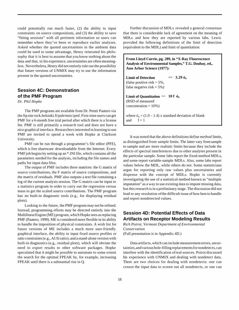
The PMF programs are available from Dr. Pentti Paatero viathe ftp site rock.helsinki.fi/pub/misc/pmf. First-time users can getPMF for a 6-month free trial period after which there is a licensefee. PMF is still primarily a research tool and does not have anice graphical interface. Researchers interested in learning to usePMF are invited to spend a week with Hopke at ClarksonUniversity.

PMF can be run through a programmer’s file editor (PFE),which is free shareware downloadable from the Internet. EveryPMF job begins by setting up an *.INI file, which contains all theparameters needed for the analysis, including the file names andpaths for input data files.

The output of PMF includes three matrices: the G matrix ofsource contributions, the F matrix of source compositions, andthe matrix of residuals. PMF also outputs a text file containing alog of the current analysis session. The G matrix can be input toa statistics program in order to carry out the regression versusmass to get the scaled source contributions. The PMF programhas no built-in diagnostic tools (e.g., for displaying residualplots).

Looking to the future, the PMF program may not be refined.Instead, programming efforts may be directed entirely into theMultilinear Engine (ME) program, which Hopke sees as replacingPMF (Paatero, 1999). ME is considered more flexible in its abilityto handle the imposition of physical constraints. A wish list forfuture versions of ME includes a much more user-friendlygraphical interface, the ability to input fixed source profiles orratio constraints (e.g., Al:Si ratio), and a stand-alone version withbuilt-in diagnostics (e.g., residual plots), which will obviate theneed to export results to other software packages. Hopkespeculated that it might be possible to automate to some extentthe search for the optimal FPEAK by, for example, increasingFPEAK until there is a substantial rise in Q.

Further discussion of MDLs revealed a general consensusthat there is considerable lack of agreement on the meaning ofMDLs and how they are reported by various labs. Lewisprovided the following definitions of the limit of detection(equivalent to the MDL) and limit of quantitation:

It was noted that the above definitions define method limits,as distinguished from sample limits. The latter vary from sampleto sample and are more realistic limits because they include theeffects of spectral interferences due to other analytes present inthe particular sample. Some labs report the fixed-method MDLs,and some report variable-sample MDLs. Also, some labs reportvalues below the MDL, while others do not. Some statisticiansargue for reporting only raw values plus uncertainties anddispense with the concept of MDLs. Hopke is currentlyinvestigating the use of a statistical method known as “multipleimputation” as a way to use existing data to impute missing data,but this research is in a preliminary stage. The discussion did notlead to any resolution of the difficult issue of how best to handleand report nondetected values.

Session 4D: Potential Effects of DataArtifacts on Receptor Modeling ResultsRich Poirot, Vermont Department of EnvironmentalConservation(Full presentation is in Appendix 4D.)

Data artifacts, which can include measurement errors, uncer-tainties, and various hole-filling replacements for nondetects, caninterfere with the identification of real sources. Poirot discussedhis experience with UNMIX and dealing with nondetect data.There are two choices for dealing with nondetects: one cancensor the input data to screen out all nondetects, or one can

From Lloyd Currie, pg. 289, in “X-Ray FluorescenceAnalysis of Environmental Samples,” T.G. Dzubay, ed.,Ann Arbor Science (1977):

Limit of Detection == 3.29 ó0

(false positive risk = 5%,false negative risk = 5%)

Limit of Quantitation == 10 f ó0

(RSD of measuredconcentration = 10%)

where ó0 = (1.0 – 1.4) x standard deviation of blankand f = 1

19

use some hole-filling techniques to replace nondetects. Theformer approach can create a small and biased subset of theoriginal data. Poirot discussed the results of using various hole-filling techniques to modify the input data for UNMIXcalculations. In the end, Poirot felt that simple replacement ofnondetect values with zeros (or some small constant) yielded themost consistent and interpretable UNMIX results.

Poirot showed a series of slides lending support to thosewho mistrust reported uncertainties and MDLs. For example, Niand As measurements at Lye Brook, VT, are totally uncorrelatedand yet

the reported uncertainties exhibit a significant positivecorrelation (top figure below). Also, he said, “although concen-trations of Ni and As are uncorrelated, their MDLs are highlycorrelated, both as a function of three methods changes indifferent time periods, and also within each of three differentreporting periods” (bottom figure below).

20

Poirot went on to say that “[this is] possibly due to commoninterferences or instrumental drift, but not due to changingambient concentrations. Generally, in most long-term measure-ment programs both ambient concentrations and detection limitsare likely to decrease over time, creating the possibility of falsepositive correlations between source activity for some elementsand lab activity for other elements.” This latter point waselegantly demonstrated by a plot of same-day, above-MDL Asconcentrations at Acadia and Mt. Rainier IMPROVE sites. Themeasured concentrations exhibit no correlation (as expectedgiven the continental distance between sites). However, same-day As MDLs for these sites are correlated, generally due to“progress” (improving detection limits over time) in the 10+ yearIMPROVE network. Poirot also provided evidence for“misquantified” MDLs for Al in IMPROVE data. He presentedsome encouraging results, which showed that despite widedifferences in data preprocessing and model input, both UNMIXand PMF identified three common sources in an IMPROVE-likedata set. However, artifacts associated with changes in Se MDLsdue to a change from PIXE to XRF analysis during the samplingperiod clearly influenced the UNMIX and PMF results indifferent ways.

Poirot concluded by saying, “Data Artifacts, includingMDLs and uncertainties as reported by labs and/or as processedby data analysts, can and do influence receptor model results.”

Session 4E: Open Discussion There was further discussion of the MDLs. It was not

known whether the EPA PM2.5 Speciation Monitoring Networkwill report the single method-based MDLs or the daily-varyingsample MDLs. Henry reconsidered his distrust of reported MDLsand uncertainties and found it to be justified. In situations whereone cannot afford to lose data due to nondetects, Henryrecommends just replacing the nondetects with zero or a smallconstant.

Important MDL-related questions include the following:How are MDL and uncertainty values determined by analyticallaboratories? Do these reported values have the same meaningat different labs or in different measurement programs? How haveanalytical methods and the resultant data changed over thecourse of a measurement program? And finally, what are the bestways of processing this information as input to different receptormodels?

In response to the question of whether or not to use massas a fitting species, Henry and Hopke expressed differentphilosophies. Henry likes to include the mass so that the totalmass is apportioned just like the species mass. Hopke hastraditionally kept the mass separate and likes to use the resultsof the mass regression analysis as an added check on thevalidity of the model results.

Henry expressed his concern that the errors reported in bothUNMIX and PMF have not been given adequate scrutiny. Hopkebelieves that the error estimates in PMF are almost certainlyoverestimates.

Several members of the audience commented on the dreadedUNMIX message informing the user that there was “no feasiblesolution” to a problem. Henry responded that rather thanviewing this as a bug or deficiency in UNMIX, it should insteadbe viewed as a valuable feature in that a bad solution is worsethan no solution.

There was some discussion about dealing with outliers.Henry relies heavily on UNMIX scatterplots to identify outliers.He urged caution in eliminating suspected outliers because, ifreal, they can provide very important information about sourcecompositions. Hopke typically does a principal componentsanalysis of the data and plots factor scores to identify outliers.The “robust mode” option in PMF automatically downweightsoutliers (but does not eliminate them) so that they do not exerttoo much influence. If the user knows that a certain sample is anoutlier (e.g., fireworks on the Fourth of July), then it is best toremove that data point before performing UNMIX or PMFanalysis.

The interpretation of source profiles remains one of thebiggest challenges in using these tools. Receptor modelingshould not be done in a vacuum. Ideally, the modeler will haveintimate knowledge of the modeled airshed, or will work closelywith someone who does. Rich Poirot suggested creating aninformal, unofficial bulletin board or site where modelers couldshare source profiles (accompanied by some descriptiveinformation) generated by UNMIX or PMF. Lewis would likemodelers to show their profiles in publications. With emphasison PM2.5, there is likely to be increased mass being apportionedto regional sources, which are typically dominated by secondaryspecies. It would be useful to compile a library of regional“fingerprints.” Such a library could be helpful in proper sourceidentification. There are some good tools such as residence timeanalysis, back-trajectory analysis, and partial source contributionfunction (PSCF) analysis for identifying and quantifying regionalimpacts. Hopke showed how PSCF was able to trace a Ni-V factorin Vermont back to residual oil combustion in the Eastern urbancorridor.

21

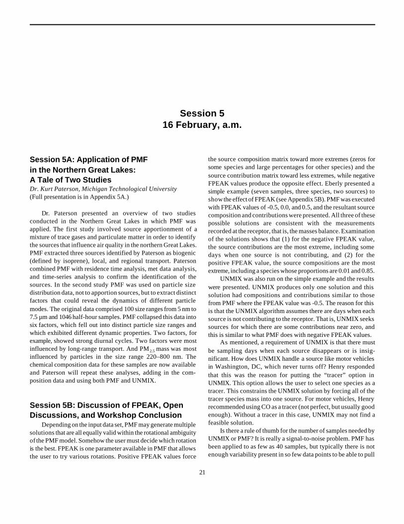
Session 516 February, a.m.

Session 5A: Application of PMFin the Northern Great Lakes:A Tale of Two StudiesDr. Kurt Paterson, Michigan Technological University(Full presentation is in Appendix 5A.)

Dr. Paterson presented an overview of two studiesconducted in the Northern Great Lakes in which PMF wasapplied. The first study involved source apportionment of amixture of trace gases and particulate matter in order to identifythe sources that influence air quality in the northern Great Lakes.PMF extracted three sources identified by Paterson as biogenic(defined by isoprene), local, and regional transport. Patersoncombined PMF with residence time analysis, met data analysis,and time-series analysis to confirm the identification of thesources. In the second study PMF was used on particle sizedistribution data, not to apportion sources, but to extract distinctfactors that could reveal the dynamics of different particlemodes. The original data comprised 100 size ranges from 5 nm to7.5 µm and 1046 half-hour samples. PMF collapsed this data intosix factors, which fell out into distinct particle size ranges andwhich exhibited different dynamic properties. Two factors, forexample, showed strong diurnal cycles. Two factors were mostinfluenced by long-range transport. And PM 2.5 mass was mostinfluenced by particles in the size range 220–800 nm. Thechemical composition data for these samples are now availableand Paterson will repeat these analyses, adding in the com-position data and using both PMF and UNMIX.

Session 5B: Discussion of FPEAK, OpenDiscussions, and Workshop Conclusion

Depending on the input data set, PMF may generate multiplesolutions that are all equally valid within the rotational ambiguityof the PMF model. Somehow the user must decide which rotationis the best. FPEAK is one parameter available in PMF that allowsthe user to try various rotations. Positive FPEAK values force

the source composition matrix toward more extremes (zeros forsome species and large percentages for other species) and thesource contribution matrix toward less extremes, while negativeFPEAK values produce the opposite effect. Eberly presented asimple example (seven samples, three species, two sources) toshow the effect of FPEAK (see Appendix 5B). PMF was executedwith FPEAK values of -0.5, 0.0, and 0.5, and the resultant sourcecomposition and contributions were presented. All three of thesepossible solutions are consistent with the measurementsrecorded at the receptor, that is, the masses balance. Examinationof the solutions shows that (1) for the negative FPEAK value,the source contributions are the most extreme, including somedays when one source is not contributing, and (2) for thepositive FPEAK value, the source compositions are the mostextreme, including a species whose proportions are 0.01 and 0.85.

UNMIX was also run on the simple example and the resultswere presented. UNMIX produces only one solution and thissolution had compositions and contributions similar to thosefrom PMF where the FPEAK value was -0.5. The reason for thisis that the UNMIX algorithm assumes there are days when eachsource is not contributing to the receptor. That is, UNMIX seekssources for which there are some contributions near zero, andthis is similar to what PMF does with negative FPEAK values.

As mentioned, a requirement of UNMIX is that there mustbe sampling days when each source disappears or is insig-nificant. How does UNMIX handle a source like motor vehiclesin Washington, DC, which never turns off? Henry respondedthat this was the reason for putting the “tracer” option inUNMIX. This option allows the user to select one species as atracer. This constrains the UNMIX solution by forcing all of thetracer species mass into one source. For motor vehicles, Henryrecommended using CO as a tracer (not perfect, but usually goodenough). Without a tracer in this case, UNMIX may not find afeasible solution.

Is there a rule of thumb for the number of samples needed byUNMIX or PMF? It is really a signal-to-noise problem. PMF hasbeen applied to as few as 40 samples, but typically there is notenough variability present in so few data points to be able to pull

22

out distinct factors. Recent work by John Ondov (PM2000Charleston Conference) has shown that by sampling with hightime resolution (half-hour) one can dramatically improve thesignal/noise for sources with temporal variability. Henry offeredthe following rule of thumb for UNMIX: 200–300 samples mayget you five sources; 2000–3000 samples may be needed toextract 9–10 sources.

How can receptor modelers take advantage of the EPASpeciation Monitoring Network now coming online? What toolsare available to interpret these data? Instead of modeling multiplespecies at a single site, one can model a single species acrossmultiple sites. In this way, one can extract spatial concentrationgradients, which, combined with wind-direction analysis, canidentify source locations. Alternatively, one can model multiplespecies at multiple sites using three-way factor analysis (Hopkeet al., 1998).

A member of the audience pointed out the discrepancies inthe UNMIX and PMF solutions for the Phoenix data, mostnotably the mass apportioned to vegetative burning in the twomodels. Are such discrepancies the result of applying differentmodels, or the result of different people interpreting the sameinformation? Hopke responded by saying that the modeler needsto tap into the local expertise to help identify important sourcesand to screen out unreasonable solutions. It is always good tocome at a problem with as many tools as possible. If one can getsimilar solutions using both PMF and UNMIX, this addsconfidence to the results.

Henry proposed a strategy that combines UNMIX and PMFand should yield defensible solutions. In this combined ap-proach, the modeler might start with UNMIX to estimate thenumber of factors and to get good starting source profiles.UNMIX profiles could be used as starting profiles for PMF, sincePMF is particularly good at finding smaller sources and includingadditional species. (This will shorten the PMF analysis since themodel does not have to start with random profiles.) Applyingother information such as wind-direction plots, one can probablycome up with 10 or more sources. The ability to look at residualsin PMF can be very helpful as a quality check at the end of themodeling process.

Kurt Paterson suggested that it would be very useful tohave thorough training tutorials for both PMF and UNMIXshowing detailed applications of the tools in actual case studies.

There was a broad discussion regarding the roles of regionalplanning bodies and state regulatory agencies in dealing withcompliance issues. Within a few years, regulatory agencies willneed to address reductions at both the regional and local levels,with the regional planning bodies probably taking the lead. Willthe state and regional agencies have the resources and theexpertise to utilize the latest modeling tools? How can PMF andUNMIX be used to separate the regional from the local sources?Can the IMPROVE and Speciation networks be combined insome way to help separate regional sources from local sources?

Henry responded that there presently exist a handful of goodtools for dealing with regional sources. The challenge is forsomeone to put these tools together and make people aware thatthey exist. Perhaps the EPA regional offices can play a role indisseminating information about these tools or providing trainingto state agencies.

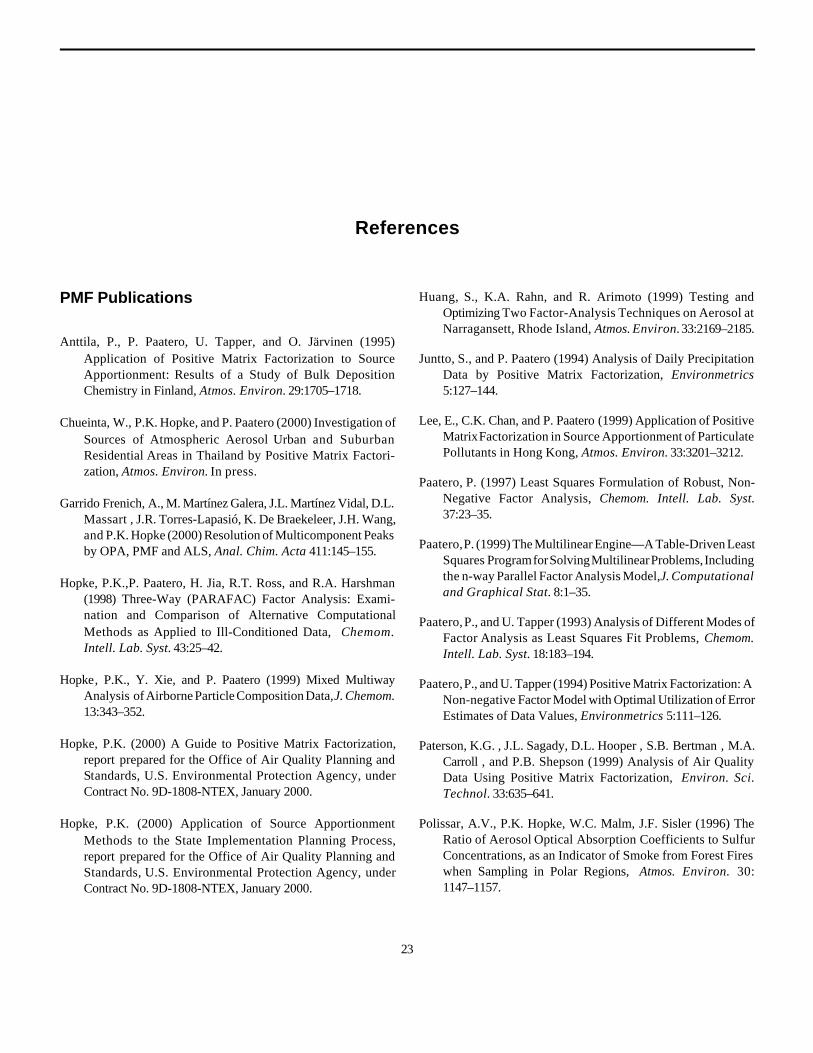
23

References

PMF Publications

Anttila, P., P. Paatero, U. Tapper, and O. Järvinen (1995)Application of Positive Matrix Factorization to SourceApportionment: Results of a Study of Bulk DepositionChemistry in Finland, Atmos. Environ. 29:1705–1718.

Chueinta, W., P.K. Hopke, and P. Paatero (2000) Investigation ofSources of Atmospheric Aerosol Urban and SuburbanResidential Areas in Thailand by Positive Matrix Factori-zation, Atmos. Environ. In press.

Garrido Frenich, A., M. Martínez Galera, J.L. Martínez Vidal, D.L.Massart , J.R. Torres-Lapasió, K. De Braekeleer, J.H. Wang,and P.K. Hopke (2000) Resolution of Multicomponent Peaksby OPA, PMF and ALS, Anal. Chim. Acta 411:145–155.

Hopke, P.K.,P. Paatero, H. Jia, R.T. Ross, and R.A. Harshman(1998) Three-Way (PARAFAC) Factor Analysis: Exami-nation and Comparison of Alternative ComputationalMethods as Applied to Ill-Conditioned Data, Chemom.Intell. Lab. Syst. 43:25–42.

Hopke, P.K., Y. Xie, and P. Paatero (1999) Mixed MultiwayAnalysis of Airborne Particle Composition Data, J. Chemom.13:343–352.

Hopke, P.K. (2000) A Guide to Positive Matrix Factorization,report prepared for the Office of Air Quality Planning andStandards, U.S. Environmental Protection Agency, underContract No. 9D-1808-NTEX, January 2000.

Hopke, P.K. (2000) Application of Source ApportionmentMethods to the State Implementation Planning Process,report prepared for the Office of Air Quality Planning andStandards, U.S. Environmental Protection Agency, underContract No. 9D-1808-NTEX, January 2000.

Huang, S., K.A. Rahn, and R. Arimoto (1999) Testing andOptimizing Two Factor-Analysis Techniques on Aerosol atNarragansett, Rhode Island, Atmos. Environ. 33:2169–2185.

Juntto, S., and P. Paatero (1994) Analysis of Daily PrecipitationData by Positive Matrix Factorization, Environmetrics5:127–144.

Lee, E., C.K. Chan, and P. Paatero (1999) Application of PositiveMatrix Factorization in Source Apportionment of ParticulatePollutants in Hong Kong, Atmos. Environ. 33:3201–3212.

Paatero, P. (1997) Least Squares Formulation of Robust, Non-Negative Factor Analysis, Chemom. Intell. Lab. Syst.37:23–35.

Paatero, P. (1999) The Multilinear Engine—A Table-Driven LeastSquares Program for Solving Multilinear Problems, Includingthe n-way Parallel Factor Analysis Model, J. Computationaland Graphical Stat. 8:1–35.

Paatero, P., and U. Tapper (1993) Analysis of Different Modes ofFactor Analysis as Least Squares Fit Problems, Chemom.Intell. Lab. Syst. 18:183–194.

Paatero, P., and U. Tapper (1994) Positive Matrix Factorization: ANon-negative Factor Model with Optimal Utilization of ErrorEstimates of Data Values, Environmetrics 5:111–126.

Paterson, K.G. , J.L. Sagady, D.L. Hooper , S.B. Bertman , M.A.Carroll , and P.B. Shepson (1999) Analysis of Air QualityData Using Positive Matrix Factorization, Environ. Sci.Technol. 33:635–641.

Polissar, A.V., P.K. Hopke, W.C. Malm, J.F. Sisler (1996) TheRatio of Aerosol Optical Absorption Coefficients to SulfurConcentrations, as an Indicator of Smoke from Forest Fireswhen Sampling in Polar Regions, Atmos. Environ. 30:1147–1157.

24

Polissar, A.V., P.K. Hopke, W.C. Malm, J.F. Sisler (1998)Atmospheric Aerosol over Alaska: 2. Elemental Compositionand Sources, J. Geophys. Res. 103:19,045–19,057.

Polissar, A.V., P.K. Hopke, P. Paatero, Y.J. Kaufman, D.K. Hall,B.A. Bodhaine, E.G. Dutton, and J.M. Harris (1999) TheAerosol at Barrow, Alaska: Long-Term Trends and SourceLocations, Atmos. Environ. 33: 2441–2458.

Ramadan, Z., X.-H. Song, P.K. Hopke (2000) Identificaton ofSources of Phoenix Aerosol by Positive Matrix Factori-zation, JAWMA. In press.

Xie, Y.-L., P.K. Hopke, and P. Paatero (1998) Positive MatrixFactorization Applied to Curve Resolution Problem, J.Chemom. 12:357–364.

Xie, Y.-L., P.K. Hopke, P. Paatero, L.A. Barrie, and S.-M. Li(1999a) Identification of Source Nature and SeasonalVariations of Arctic Aerosol by the Multilinear Engine,Atmos. Environ. 33:2549–2562.

Xie, Y.-L., P.K. Hopke, and P. Paatero (1999c) CalibrationTransfer as a Data Reconstruction Problem, Anal. Chim.Acta 384:193–205.

Xie, Y. L., P. Hopke, P. Paatero, L.A. Barrie, and S.M. Li (1999b)Identification of Source Nature and Seasonal Variations ofArctic Aerosol by Positive Matrix Factorization, J. Atmos.Sci. 56:249–260.

Yakovleva, E., P.K. Hopke, and L. Wallace (1999) ReceptorModeling Assessment of PTEAM Data, Environ. Sci.Technol. 33:3645–3652.

UNMIX and SAFER (the ParentModel of UNMIX) Publications

Henry, R.C. and B.- M. Kim (1989) A Factor Analysis Model withExplicit Physical Constraints, Transactions Air Pollut.Control Assoc. 14:214–225.

Henry, R.C., and B.-M. Kim (1990) Extension of Self-ModelingCurve Resolution to Mixtures of More Than Three Com-ponents. Part 1: Finding the Basic Feasible Region,Chemom. Intell. Lab. Syst. 8:205–216.

Henry, R.C., C.W. Lewis, J.F. Collins (1994) Vehicle-RelatedHydrocarbon Source Composition from Ambient Data: The

GRACE/SAFER Method, Environ. Sci. Technol. 28:823–832.

Henry, R.C. (1997) History and Fundamentals of Multivariate AirQuality Receptor Models, Chemom. Intell. Lab. Syst.37:525–530.

Henry, R.C., and C. Spiegelman (1997) Reported Emissions ofVolatile Organic Compounds are not Consistent withObservations, Proc. Nat. Acad. Sci. 94:6596–6599.

Henry, R.C., E.S. Park, and C.H. Spiegelman (1999) Comparing aNew Algorithm with the Classic Methods for Estimating theNumber of Factors, Chemom. Intell. Lab. Syst. 48:91–97.

Kim, B.-M., and R.C. Henry (1999) Extension of Self-ModelingCurve Resolution to Mixtures of More Than ThreeComponents. Part 2: Finding the Complete Solution,Chemom. Intell. Lab. Syst. 49:67–77.

Kim, B.-M., and R.C. Henry (2000) Application of the SAFERModel to Los Angeles PM10 Data, Atmos. Environ.34:1747–1759.

Kim, B.-M., and R.C. Henry (2000) Extension of Self-ModelingCurve Resolution to Mixtures of More Than ThreeComponents. Part 3, Chemom. Intell. Lab. Syst. Submitted.

Park, E.S., C. Spiegelman, and R.C. Henry (2000) BilinearEstimation of Pollution Source Profiles and Amounts byUsing Receptor Models, Communications in Statistics,Simulation & Computation, 29(3). In press.

25

UNMIX/PMF Receptor Modeling Workshop Attendees14–16 February 2000U.S. EPA, RTP, NC

Name Affiliation Phone E-mail Mailing Address

Charles Lewis U.S. EPA 919-541-3154 lewis.charlesw@epa.gov U.S. EPANERL (MD-47)RTP, NC 27711

Philip K. Hopke Clarkson University 315-268-3861 hopkepk@clarkson.edu Clarkson UniversityBox 5810Potsdam, NY 13695-5810

Ron Henry University of SouthernCalifornia, Los Angeles

213-740-0596 rhenry@usc.edu

John Bachmann U.S. EPA 919-541-5359 jbachmann@epa.gov U.S. EPANERL (MD-10)RTP, NC 27711

Scott Kegler U.S. EPA 919-541-4906 kegler.scott@epa.gov U.S. EPANERL (MD-52)RTP, NC 27711

Mark Hubble Arizona DEQ 602-207-4481 mh1@ev.state.az.us Arizona DEQ3033 N. Central Ave.Phoenix, AZ 85012

Lara Autry U.S. EPA 919-541-5544 autry.lara@epa.gov U.S. EPANERL (MD-14)RTP, NC 27711

Donna Kenski U.S. EPA 312-886-7894 kenski.donna@epa.gov EPA Region 577 W. Jackson Blvd.Chicago, IL 60604

Tom Pace U.S. EPA 919-541-5634 pace.tom@epa.gov U.S. EPANERL (MD-14)RTP, NC 27711

Larry Cox U.S. EPA 919-541-2648 cox.larry@epamail.epa.gov U.S. EPANERL (MD-75)RTP, NC 27711

N. Dean Smith U.S. EPA 919-541-2708 smith.dean@epa.gov U.S. EPANERL (MD-61)RTP, NC 27711

Basil Coutant U.S. EPA 919-541-5028 coutant.basil@epa.gov U.S. EPANERL (MD-14)RTP, NC 27711

Alan Vette U.S. EPA 919-541-1378 vette.alan@epa.gov U.S. EPANERL (MD-56)RTP, NC 27711

Anne Rea U.S. EPA 919-541-0053 rea.anne@epa.gov U.S. EPANERL (MD-56)RTP, NC 27711

Name Affiliation Phone E-mail Mailing Address

26

Teri Conner U.S. EPA 919-541-3157 conner.teri@epa.gov U.S. EPANERL (MD-46)RTP, NC 27711

Tom Braverman U.S. EPA 919-541-5383 braverman.tom@epa.gov U.S. EPANERL (MD-14)RTP, NC 27711

Allan Marcus U.S. EPA 919-541-0636 marcus.allan@epa.gov U.S. EPANERL (MD-52)RTP, NC 27711

Shao-Hang Chu U.S. EPA 919-541-5382 chu.shao-hang@epa.gov U.S. EPANERL (MD-15)RTP, NC 27711

Ned Meyer U.S. EPA 919-541-5594 meyer.ned@epa.gov U.S. EPAOAQPS (MD-14)RTP, NC 27711

Peter Frechtel U.S. EPA 919-541-1173 frechtel.peter@epa.gov U.S. EPAOAQPS (MD-14)RTP, NC 27711

Eugene Kim University ofWashington

206-526-2909 ugene@u.washington.edu

Tom Rosendahl U.S. EPA 919-541-5314 rosendahl.tom@epa.gov U.S. EPAOAQPS (MD-15)RTP, NC 27711

Cynthia HowardReed

U.S. EPA 703-648-5222 howard.cynthia@epa.gov U.S. EPA12201 Sunrise Valley Dr.555 National CenterReston, VA 20192

Barbara Parzygnat U.S. EPA 919-541-5474 parzygnat.barbara@epa.gov U.S. EPAOAQPS (MD-14)RTP, NC 27711

Bob Willis ManTech Environmental 919-541-2809 willis.robert@epa.gov ManTech EnvironmentalP.O. Box 12313RTP, NC 27709

Kaz Ito New York University 914-731-3540 kaz@env.med.nyu.edu New York University, Env.Med.57 Old Forge Rd.Tuxedo, NY 10987

Shaibal Mukerjee U.S. EPA 919-541-1865 mukerjee.shaibal@epa.gov U.S. EPANERL (MD-47)RTP, NC 27711

John Langstaff 919-967-6649 jlangstaff@mindspring.com 1105 Valley Park Dr.Chapel Hill, NC 27514

Melissa Gonzales U.S. EPA 919-966-7549 gonzales.melissa@epa.gov U.S. EPAMD-58ARTP, NC 27711

Name Affiliation Phone E-mail Mailing Address

27

Tom Coulter U.S. EPA 919-541-0832 coulter.tom@epa.gov U.S. EPAMD-47RTP, NC 27711

Rich Poirot 802-211-3807 richpo@dec.anr.state.vt.us 103 South Main St.Waterbury, VT 05671

Steve Fudge 919-933-9501 fudge.steve@ecrweb.com 1129 Weaver Dairy Rd.Chapel Hill, NC 27514

Shelly Eberly U.S. EPA 919-541-4128 eberly.shelly@epa.gov U.S. EPANERL (MD-14)RTP, NC 27711

Jong Hoon Lee Rutgers University 732-932-0306 jhlee@aesop.rutgers.edu Rutgers University14 College Farm Rd.New Brunswick, NJ 08901

Barbara Turpin Rutgers University 732-932-9540 turpin@aesop.rutgers.edu Rutgers University14 College Farm Rd.New Brunswick, NJ 08901

Kurt Paterson Michigan TechUniversity

906-487-3495 Paterson@mtu.edu Michigan Tech UniversityDept. Civil & Env.Engineering1400 Townsend DriveHoughton, MI 49931