workshop prediction analysis, post ... - the engineering lab

The Engineering LabNastran SOL 200 questions? Email me: christian@ the-engineering-lab.com

Workshop – Prediction Analysis, Post-BucklingAN MSC NASTRAN MACHINE LEARNING WEB APP TUTORIAL

2The Engineering LabNastran SOL 200 questions? Email me: christian@ the-engineering-lab.com 2

Goal: Prediction AnalysisThis tutorial consists of multiple parts

1. Configuring The Problem Statement◦ In this tutorial, we configure the parameters and the responses to monitor.

2. Configuring Multiple Batch Runs◦ This section discusses how to configure and execute multiple MSC Nastran runs.

3. Performing Predictions◦ Gaussian process (GP) regression is used to train a surrogate model.

◦ Two (2) artificial samples are manually added to the training data, which results in a “spiked” surrogate model. A solution to the “spiked” surrogate model is demonstrated.

◦ Excel is used to manually customize the training data.

4. Creating Plots with the HDF5 Explorer◦ The HDF5 Explorer web app is used to create load vs. displacement plots.


1. Perform a post-buckling analysis for different values of Ks

2. Create a Load vs. Displacement plot for node 2

Details of the Structural Model

P, q

11

x

y100.

14.

12.

10.

8.

6.

4.

2.

0

0

0.5 1.0 1.5 2.0 2.5 3.0

q

.235

1.765 2.16

18.

16.

2

1.Ks

P

Ks 6.0

Ks 3.0

EA = 107P, q

11

x

y100.

14.

12.

10.

8.

6.

4.

2.

0

0

0.5 1.0 1.5 2.0 2.5 3.0

q

.235

1.765 2.16

18.

16.

2

1.Ks

P

Ks 6.0

Ks 3.0

EA = 107


Details of the Structural Model

P, q

11

x

y100.

14.

12.

10.

8.

6.

4.

2.

0

0

0.5 1.0 1.5 2.0 2.5 3.0

q

.235

1.765 2.16

18.

16.

2

1.Ks

P

Ks 6.0

Ks 3.0

EA = 107P, q

11

x

y100.

14.

12.

10.

8.

6.

4.

2.

0

0

0.5 1.0 1.5 2.0 2.5 3.0

q

.235

1.765 2.16

18.

16.

2

1.Ks

P

Ks 6.0

Ks 3.0

EA = 107


P, q

11

x

y100.

14.

12.

10.

8.

6.

4.

2.

0

0

0.5 1.0 1.5 2.0 2.5 3.0

q

.235

1.765 2.16

18.

16.

2

1.Ks

P

Ks 6.0

Ks 3.0

EA = 107

Problem Statement

Monitored Responses

r1: Displacement at node 2, y component, max displacement for time steps

r2: Displacement at node 2, y component, at time step .1

r3: Load at node 2, y component, max load for time steps

r4: Load at node 2, y component, at time step .1

Design Variables

x1: K of PELAS 20 Note that K is displayed as Ks in the figure

.1 < x1 < 10.0

Samples• Batch set 1 – 10 run LHS Design


Problem Statement, ContinuedThe responses defined in this tutorial correspond to points on the displacement plot◦ r1: The minimum point of

displacement is tracked◦ r2: The displacement at time step

.1 is tracked

Surrogate Models ◦ When the surrogate model is

created for r1, the surrogate model is used to predict the max displacement.

◦ When the surrogate model is created for r2, the model is used to predict the displacement only at time step .1.

r2

r1


Problem Statement, ContinuedThe responses defined in this tutorial correspond to points on the applied load plot◦ r3: The minimum point of applied

load is tracked◦ r4: The applied load at time step .1 is

tracked

Surrogate Models ◦ A surrogate model is not necessary for

the applied load since the loading is the same for all samples.

◦ The applied load responses are monitored so that the HDF5 Explorer automatically builds the applied load plot.

◦ With separate displacement and load plots, the HDF5 Explorer is used to create a combined Load vs. Displacement plot.

r4

r3

The Engineering Lab 8Nastran SOL 200 questions? Email me: [email protected]

Contact mechristian@ the-engineering-lab.com• Nastran SOL 200 training

• Nastran SOL 200 questions

• Structural optimization questions

• Access to the SOL 200 Web App


The Appendix includes information regarding the following:◦ How to import and edit previous files

◦ What is Gaussian Process Regression?

More Information Available in the Appendix

10The Engineering LabNastran SOL 200 questions? Email me: christian@ the-engineering-lab.com

Tutorial


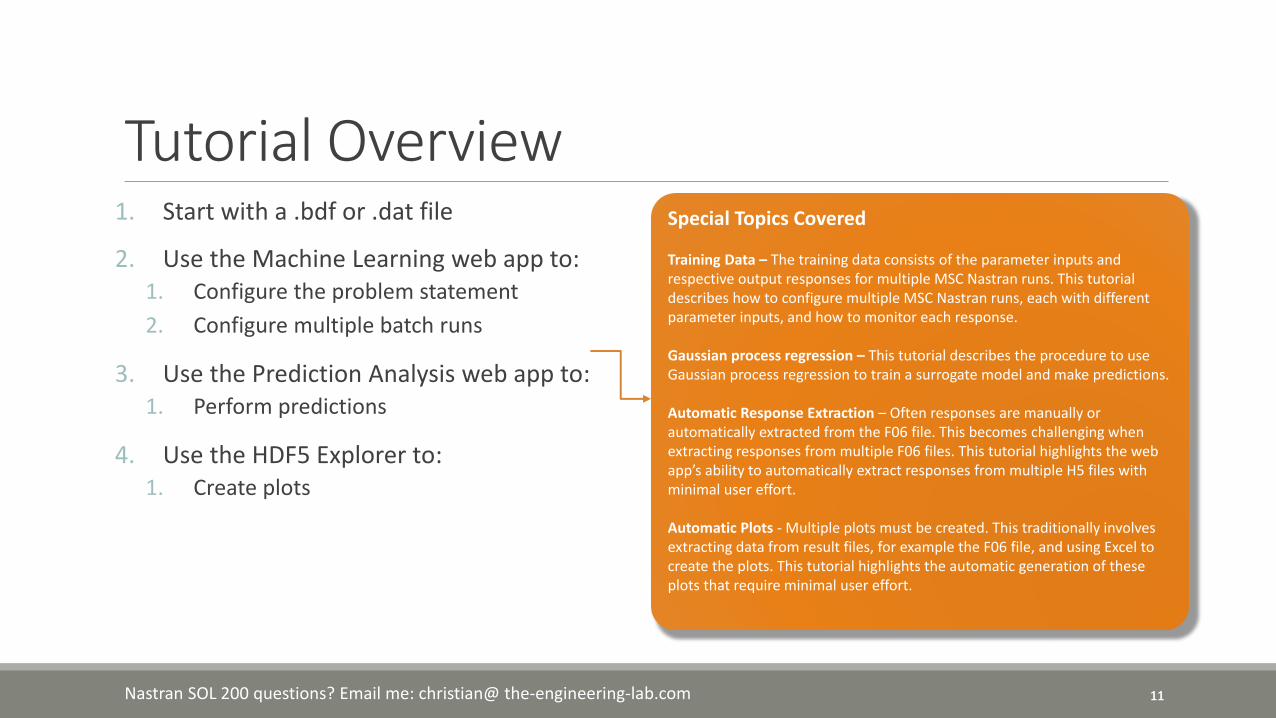
Tutorial Overview1. Start with a .bdf or .dat file

2. Use the Machine Learning web app to:1. Configure the problem statement

2. Configure multiple batch runs

3. Use the Prediction Analysis web app to:1. Perform predictions

4. Use the HDF5 Explorer to:1. Create plots

Special Topics Covered

Training Data – The training data consists of the parameter inputs and respective output responses for multiple MSC Nastran runs. This tutorial describes how to configure multiple MSC Nastran runs, each with different parameter inputs, and how to monitor each response.

Gaussian process regression – This tutorial describes the procedure to use Gaussian process regression to train a surrogate model and make predictions.

Automatic Response Extraction – Often responses are manually or automatically extracted from the F06 file. This becomes challenging when extracting responses from multiple F06 files. This tutorial highlights the web app’s ability to automatically extract responses from multiple H5 files with minimal user effort.

Automatic Plots - Multiple plots must be created. This traditionally involves extracting data from result files, for example the F06 file, and using Excel to create the plots. This tutorial highlights the automatic generation of these plots that require minimal user effort.


SOL 200 Web App for MSC NastranCapabilities Benefits

• 200+ error validations (real

time)

• Web browser accessible

• Automated creation of

entries (real time)

• Automatic post-processing

• 50+ tutorials

Web Apps for SOL 200Pre/post for MSC Nastran SOL 200. Support for size, topology, topometry and topography.

Machine Learning Web AppBayesian Optimization for nonlinear response optimization (SOL 400, 106, and 129)

MSC Apex Post Processing SupportView the newly optimized model after an optimization

Multi-model Optimization Web AppPre/post for multi model optimization

HDF5 Explorer Web AppCreate XY plots using data from the H5 file

Prediction Analysis Web AppGaussian process regression to predict output of MSC Nastran without time consuming analyses


Configuring The Problem Statement


Before Starting1. Ensure the Downloads directory is

empty in order to prevent confusion with other files

1

• Throughout this workshop, you will be working with multiple file types and directories such as:

• .bdf/.dat• nastran_working_directory• .f06, .log, .pch, .h5, etc.

• To minimize confusion with files and folders, it is encouraged to start with a clean directory.


Go to the User’s Guide1. Click on the indicated link

• The necessary BDF files for this tutorial are available in the Tutorials section of the User’s Guide.

1


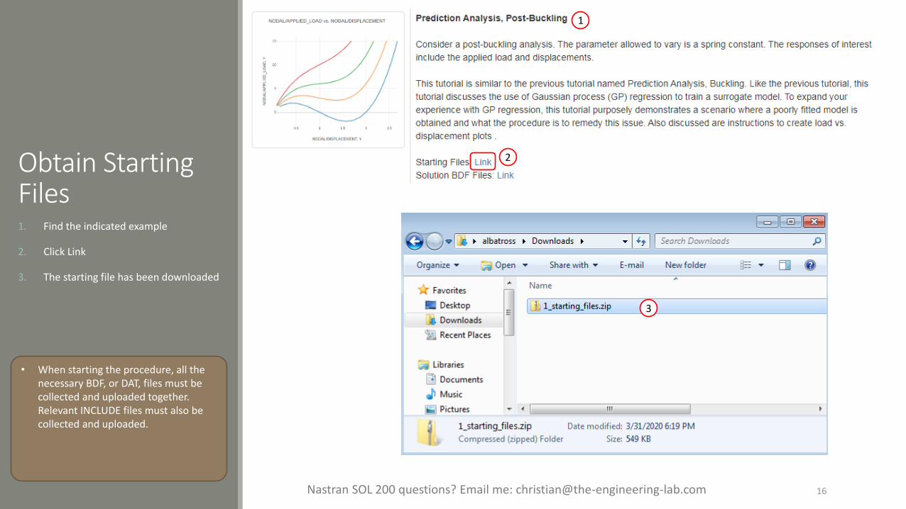
Obtain Starting Files1. Find the indicated example

2. Click Link

3. The starting file has been downloaded

1

2

3

• When starting the procedure, all the necessary BDF, or DAT, files must be collected and uploaded together. Relevant INCLUDE files must also be collected and uploaded.


Obtain Starting Files1. Right click on the zip file

2. Select Extract All…

3. Click Extract

4. The starting files are now available in a folder

• The starting files for this tutorial are contained in a ZIP file and must be extracted as shown.

1

2

3

4

4


Create the Starting H5 FileA starting H5 file must be created. This H5 file will be used to configure the responses later on.

1. Double click the MSC Nastran desktop shortcut

2. Navigate to the directory named 1_starting_files

3. Select the indicated file

4. Click Open

5. Click Run

6. The starting H5 file is created

1

3

5

4

2

6


Use the same MSC Nastran version throughout this exercise

The following applies if you have multiple versions of MSC Nastran installed.

To ensure compatibility, use the same MSC Nastran version throughout this exercise. For example, scenario 1 is OK but scenario 2 is NOT OK.

• Scenario 1 - OK• MSC Nastran 2021 is used to create the starting H5 file.• MSC Nastran 2021 is used for each run during Machine Learning or Parameter

study.• Scenario 2 – NOT OK

• MSC Nastran 2018.2 is used to create the starting H5 file.• MSC Nastran 2021 is used for each run during Machine Learning or Parameter

study.

Using the same MSC Nastran version is critical for consistent response extraction from the H5 file. A response configured for Nastran version X may not match in Nastran version Y, which leads to unsuccessful response extraction from the H5 files. The goal is to make sure all H5 files generated are from the same MSC Nastran version.


Open the Correct Page1. Click on the indicated link

• MSC Nastran can perform many optimization types. The SOL 200 Web App includes dedicated web apps for the following:

• Size, Topometry and Global Optimization

• Topology Optimization• Multi Model Optimization• Machine Learning

• The web app also features the HDF5 Explorer, a web application to extract results from the H5 file type.

1


Select BDF Files1. Click Select files

2. Select the indicated files

3. Click Open

4. Click Upload files

2

3

1

4


Parameters1. Set the following fields as parameters

• x1: The spring stiffness of PELAS 20

2. Parameters have been created for the selected fields

3. For each parameter, use the following settings:

• Low: .1

• High: 10.

• Bulk data entries will always be displayed in the small field format.

• Only fields that include decimal points can be selected as parameters.

1

2

3


Responses1. Click Responses

2. Click Select files

3. Select the indicated file

4. Click Open


• On this page, the H5 file is uploaded to the web app.

3

4

1

2

5


Adjust the Column Width1. Optional - Use at your liking the buttons at

the top right hand corner to adjust the width of the left and right columns

1


Select Responses1. Select the following dataset:

NODAL/DISPLACEMENT

2. For the Grid Identifier, select 2

3. Select the indicated cells

4. The newly created Response to Monitor are listed as r1 and r2

5. Adjust the horizontal bar to make the following column visible: Monitor the maximum or minimum […]

6. Configure the following setting for response r1

1. Monitor the maximum or minimum […]: Yes


1. Monitor the maximum or minimum […]: No

• Any cell that includes a single decimal point can be set as a response to monitor.

• For this example, the displacement, y component, at grid 2 has been set as a monitored response.

3

4

1

6

72

5


Select Responses1. Select the following dataset:

NODAL/APPLIED_LOAD

2. For the Grid Identifier, select 2

3. Select the indicated cells

4. The newly created Response to Monitor are listed as r3 and r4

5. Adjust the horizontal bar to make the following column visible: Monitor the maximum or minimum […]


1. Monitor the maximum or minimum […]: Yes


1. Monitor the maximum or minimum […]: No

• Any cell that includes a single decimal point can be set as a response to monitor.

• For this example, the applied load, y component, at grid 2 has been set as a monitored response.

3

6

1

24

7

5


Configuring Multiple Batch Runs


SamplesIn the following slides, we will configure 1 batch to run.

Batch File Name Number of Runs Purpose

1 nastran_working_directory.zip 10 The data from these 10 runs is used to train the surrogate model.

• For problems with 1-5 parameters, usually 10 runs per parameter is sufficient. This example purposely uses 20 runs (20 runs per parameter) to demonstrate an issue. The issue is discussed later in this tutorial.


1

2

Samples1. Click Samples

2. Ensure the following design is selected: Latin Hypercube, Reproducible

3. Set Number of Samples to 10

4. The samples have been updated, note that samples 1, 2, 3, …, 10 are visible

5. The indicated controls can be used to display the other samples

5

43


Download1. Click Download

2. Click Download BDF Files

3. A new ZIP file has been downloaded

3

2

1


Start Desktop App1. Right click on the indicated file

2. Click Extract All

3. Click Extract on the following window

1

3

2

• Always extract the contents of the ZIP file to a new, empty folder.


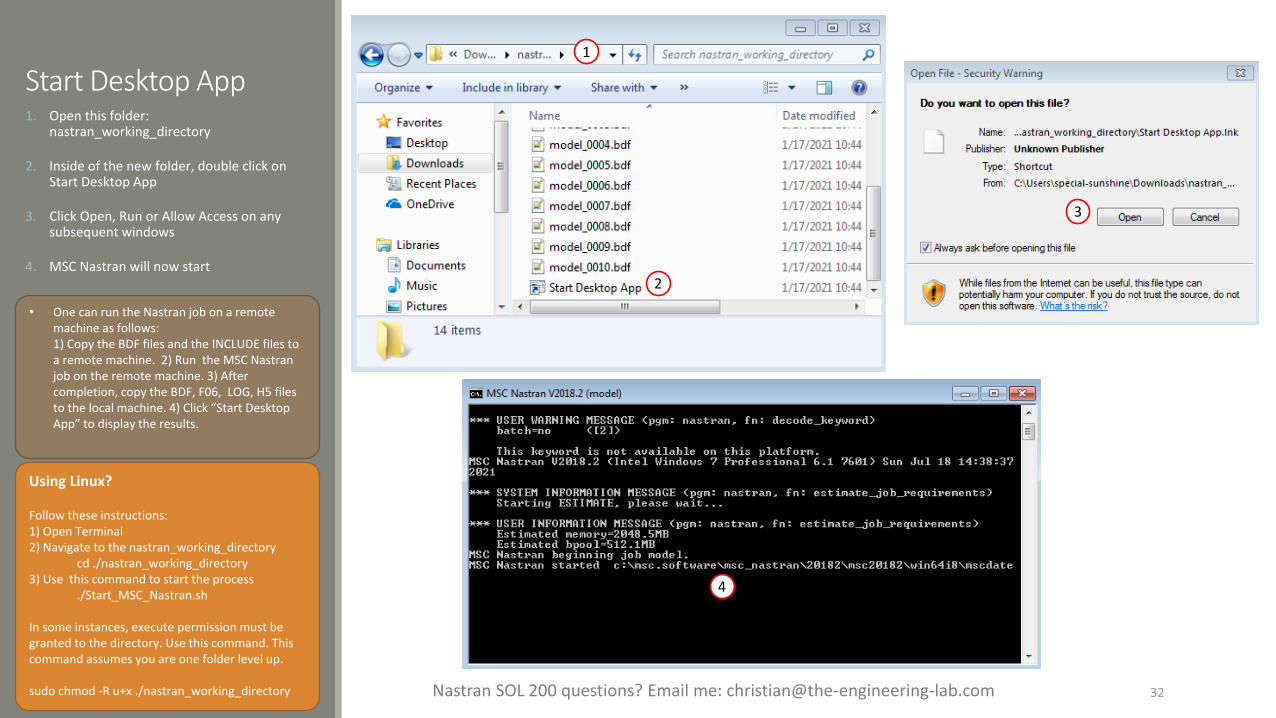
1. Open this folder: nastran_working_directory

2. Inside of the new folder, double click on Start Desktop App

3. Click Open, Run or Allow Access on any subsequent windows

4. MSC Nastran will now start2

3

4

Start Desktop App

Using Linux?

Follow these instructions:1) Open Terminal2) Navigate to the nastran_working_directory

cd ./nastran_working_directory3) Use this command to start the process

./Start_MSC_Nastran.sh

In some instances, execute permission must be granted to the directory. Use this command. This command assumes you are one folder level up.

sudo chmod -R u+x ./nastran_working_directory

• One can run the Nastran job on a remote machine as follows: 1) Copy the BDF files and the INCLUDE files to a remote machine. 2) Run the MSC Nastran job on the remote machine. 3) After completion, copy the BDF, F06, LOG, H5 files to the local machine. 4) Click “Start Desktop App” to display the results.

1


Status• While MSC Nastran is running, a status

page will show the current state of MSC Nastran


Review Results1. A window appears asking to start the HDF5

Explorer

2. Click Skip to not open the HDF5 Explorer

2

1


Review Results1. The Monitored Responses web app is

opened

2. The value of each response and for each sample is displayed in a bar chart

3. A table lists the values for each response and sample.

1

A. The table titled Monitored Response can be interacted with. Each column in the table contains filters. Once a filter is modified, the Bar Chart will instantly update.

B. Additional functions include the ability to highlight the MAX and MIN bars, download a CSV file and reset the filters.

2

3

A

B


Review Results1. The monitored responses are contained in

the CSV file named app_monitored_responses.csv

The responses in this CSV file will be use to train the surrogate model.

1


Performing Predictions


Prediction Analysis Web App1. Return to the Machine Learning web app

2. Click Results

3. Click Prediction Analysis

4. The Prediction Analysis web app is now open

5. Ensure it says Connected

1 2

3

4

5


Training Data1. Navigate to the Training and Testing Data

section

2. Delete any previous table data by clicking the four (4) buttons named Delete all rows

• x_training, y_training - This specifies the x inputs and y outputs used to train the surrogate model.

• x_testing, y_testing - This specifies the x inputs and y outputs used to calculate the Normalized Root Mean Square Error (NRMSE) between the predicted values and actual MSC Nastran responses. This testing data is option.

• x_prediction – The x inputs at which to make predictions.

2

1


Training Data1. Navigate to the section titled x_training


3. Navigate to the folder named nastran_working_directory which contains data for 10 runs

4. Select the file app.config

5. Click Open

6. Click Import

7. The table is now loaded with the x inputs for all 10 runs

1

2

3

4

5

6 7


Training Data1. Navigate to the section titled y_training


3. Navigate to the folder named nastran_working_directory which contains data for 10 runs

4. Select the file app_monitored_responses.csv

5. Click Open

6. Click Import

7. The table is now loaded with the y outputs (monitored responses) for all 10 runs

8. Note that responses r1_1, r1_2, … r3_24 contain characters instead of numbers. These characters will fail the regression and must be removed from the training data.

1

2

3

4

5

6 7

8

• Why do responses r_1, r1_2, …, r3_24 contain characters? The original FE model uses an time step procedure that varies for each sample. For example, if you are monitoring the response at time step 1.0, sample 1 may have only time step 1.1 and sample 2 may have only time step .9. Since sample 1 and 2 do not have a response corresponding time step 1.0, the extracted response is reported as “None -The response could not be found in the H5.” Training data should only contain number values. Non-number data should be removed from the training data.


Training Data1. For x_training click Export to download a

CSV file

2. For y_training click Export to download a CSV file

1

2


Custom Training Data with Excel and CSV Files1. CSV files have been download for the

training data (x inputs and y outputs)

1


Custom Training Data with Excel and CSV FilesTwo (2) artificial samples are added manually with Excel.

1. Open the file yTraining.csv in Excel

2. Delete the following response columns: r1_1, r1_2, …, r3_24. The only column that should remain are: sample, y1, y2, y3, y4.

3. Add sample 11 with the following response values

• y1: -100

• Y2: -1

• y3: -15

• y4: -1.5

4. Add sample 12 with the following response values

• y1: -90

• Y2: -0.9

• y3: -15

• y4: -1.5

5. Click Save

5 1

3

2

4


Custom Training Data with Excel and CSV Files1. Open the file xTraining.csv in Excel

2. Add a new sample and x1 value

• sample: 11

• x1: .001

3. Add a new sample and x1 value

• sample: 12

• x1: .002

4. Click Save

1

2

4

3


Training Data1. Navigate to the Training and Testing Data

section

2. Delete any previous table data by clicking the four (4) buttons named Delete all rows

2

1

• x_training, y_training - This specifies the x inputs and y outputs used to train the surrogate model.

• x_testing, y_testing - This specifies the x inputs and y outputs used to calculate the Normalized Root Mean Square Error (NRMSE) between the predicted values and actual MSC Nastran responses. This testing data is optional.

• x_prediction – The x inputs at which to make predictions.


Training Data1. Navigate to the section titled x_training


3. Navigate to the folder that contains the CSV files

4. Select the file xTraining.csv

5. Click Open

6. Click Import

7. The table is now loaded with the x inputs for 12 samples

8. Click Page 2

9. Ensure samples 11 and 12 are present

1

2

3

4

5

6 7

8

9


Training Data1. Navigate to the section titled y_training


3. Navigate to the folder that contains the CSV files

4. Select the file yTraining.csv

5. Click Open

6. Click Import

7. The table is now loaded with the y outputs (monitored responses) for 12 samples

8. Click Page 2

9. Ensure samples 11 and 12 are present and responses y1, y2, y3 and y4 are present

1

2

3

4

5

6 7

8

9


Perform Regression1. Click Perform Regression and the surrogate

model will be fitted

2. The regression is complete when the following status message is visible:

• Process complete

1

2


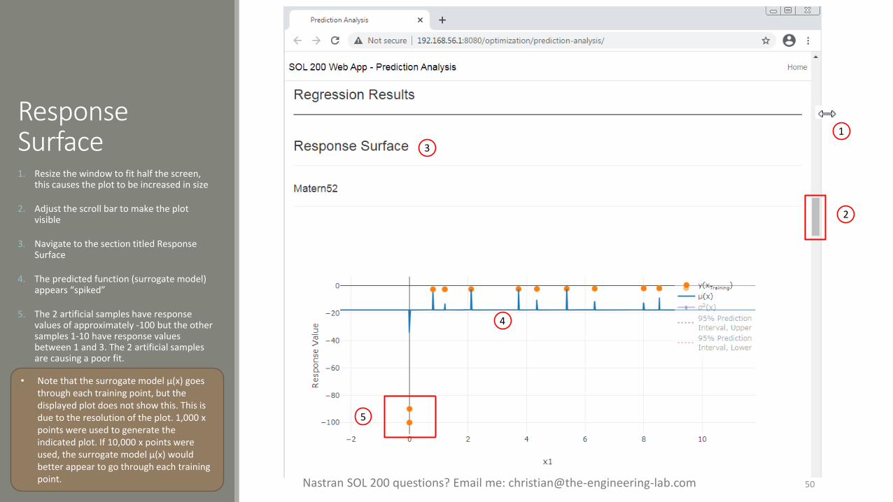
Response Surface1. Resize the window to fit half the screen,

this causes the plot to be increased in size

2. Adjust the scroll bar to make the plot visible

3. Navigate to the section titled Response Surface

4. The predicted function (surrogate model) appears “spiked”

5. The 2 artificial samples have response values of approximately -100 but the other samples 1-10 have response values between 1 and 3. The 2 artificial samples are causing a poor fit.

5

1

2

3

4

• Note that the surrogate model μ(x) goes through each training point, but the displayed plot does not show this. This is due to the resolution of the plot. 1,000 x points were used to generate the indicated plot. If 10,000 x points were used, the surrogate model μ(x) would better appear to go through each training point.


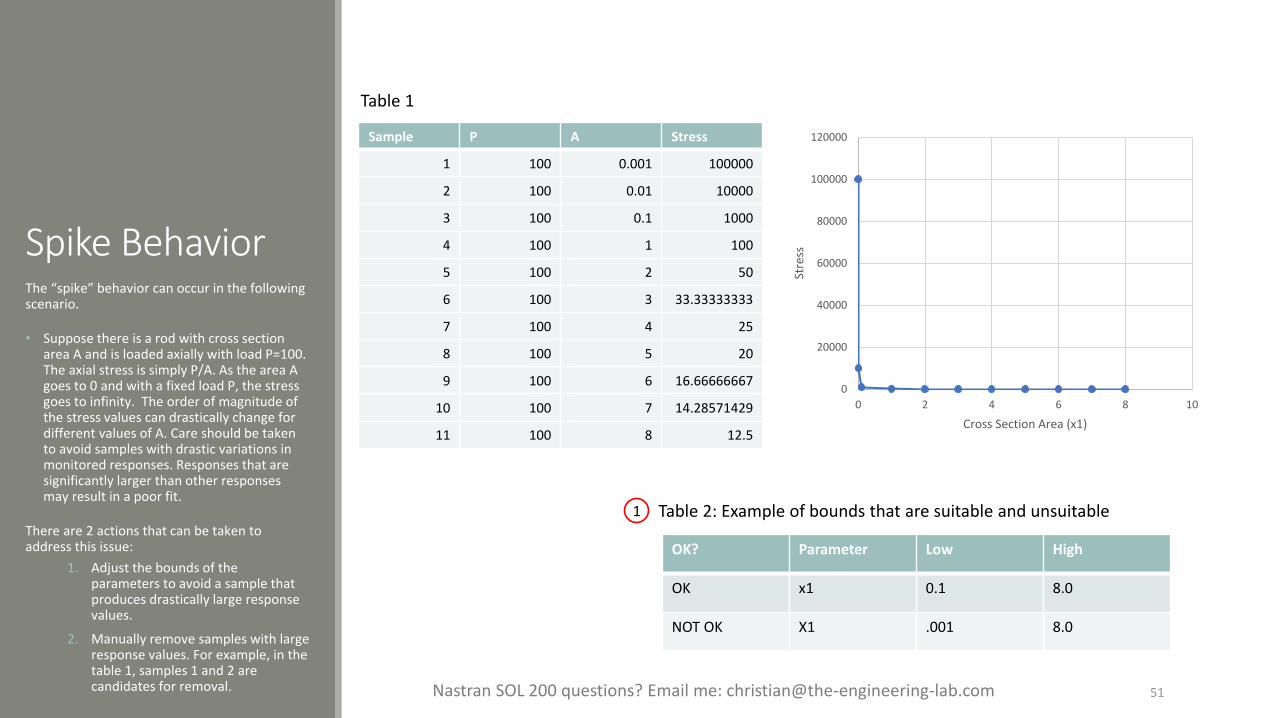
Spike BehaviorThe “spike” behavior can occur in the following scenario.

• Suppose there is a rod with cross section area A and is loaded axially with load P=100. The axial stress is simply P/A. As the area A goes to 0 and with a fixed load P, the stress goes to infinity. The order of magnitude of the stress values can drastically change for different values of A. Care should be taken to avoid samples with drastic variations in monitored responses. Responses that are significantly larger than other responses may result in a poor fit.

There are 2 actions that can be taken to address this issue:

1. Adjust the bounds of the parameters to avoid a sample that produces drastically large response values.

2. Manually remove samples with large response values. For example, in the table 1, samples 1 and 2 are candidates for removal.

0

20000

40000

60000

80000

100000

120000

0 2 4 6 8 10

Stre

ss

Cross Section Area (x1)

Sample P A Stress

1 100 0.001 100000

2 100 0.01 10000

3 100 0.1 1000

4 100 1 100

5 100 2 50

6 100 3 33.33333333

7 100 4 25

8 100 5 20

9 100 6 16.66666667

10 100 7 14.28571429

11 100 8 12.5

OK? Parameter Low High

OK x1 0.1 8.0

NOT OK X1 .001 8.0

Table 2: Example of bounds that are suitable and unsuitable1

Table 1


Variance1. Navigate to the section titled Variance

2. The “spike” behavior can be inferred from the variance plot. Very tall and leveled bars is indication of the “spike” behavior.

2

1

• In this tutorial, variance (𝜎2) is used to gauge the prediction uncertainty. Sometimes, you will see this prediction uncertainty expressed as the standard deviation (𝜎).


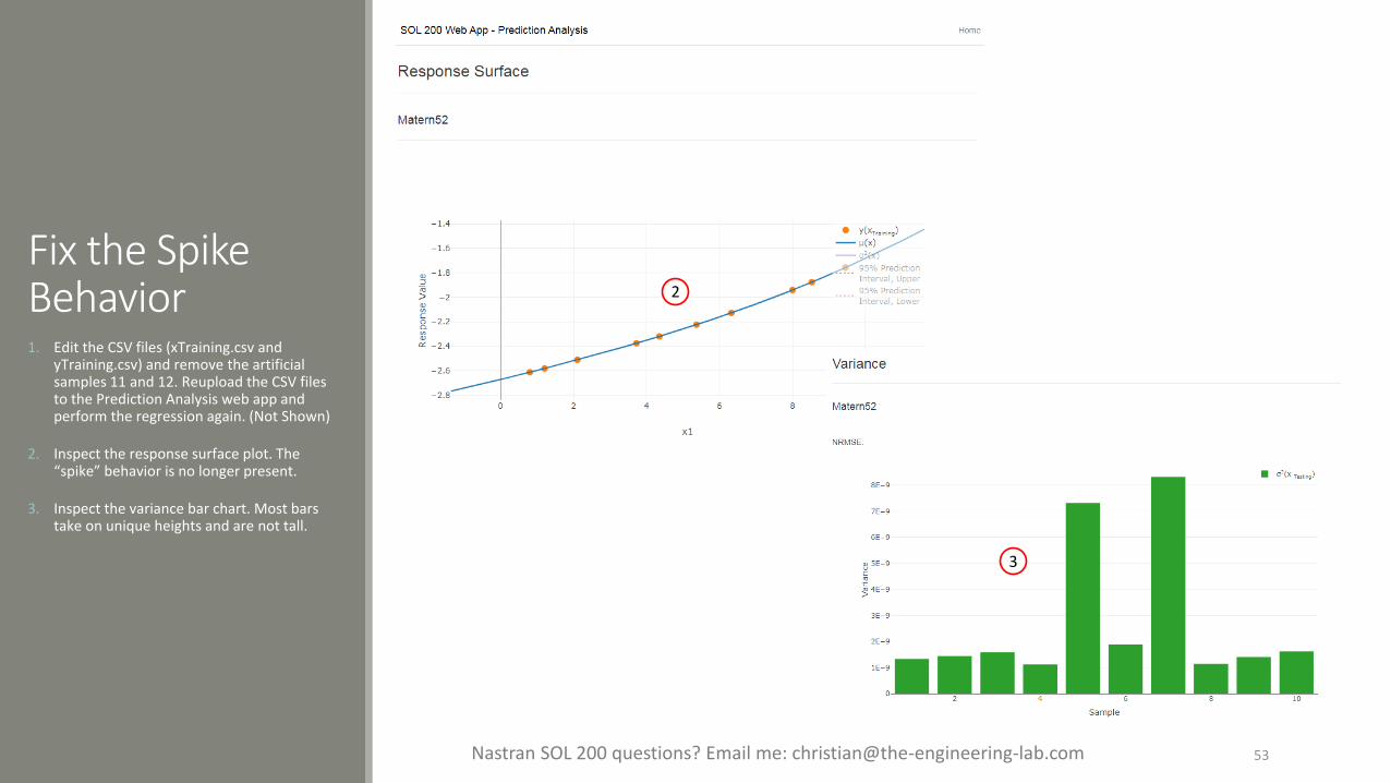
Fix the Spike Behavior1. Edit the CSV files (xTraining.csv and

yTraining.csv) and remove the artificial samples 11 and 12. Reupload the CSV files to the Prediction Analysis web app and perform the regression again. (Not Shown)

2. Inspect the response surface plot. The “spike” behavior is no longer present.

3. Inspect the variance bar chart. Most bars take on unique heights and are not tall.

2

3


Creating Plots with the HDF5 Explorer


Start Desktop App1. Open this folder:

nastran_working_directory

2. Inside of the new folder, double click on Start Desktop App

3. Click Open, Run or Allow Access on any subsequent windows

2

3

Using Linux?

Follow these instructions:1) Open Terminal2) Navigate to the nastran_working_directory

cd ./nastran_working_directory3) Use this command to start the process

./Start_MSC_Nastran.sh

In some instances, execute permission must be granted to the directory. Use this command. This command assumes you are one folder level up.

sudo chmod -R u+x ./nastran_working_directory

1


Name of Web App Purpose Description

Monitored Responses • The response value from each sample can be compared.

• After each MSC Nastran analysis, the response values are extracted from the H5 file and contained in a file named app_monitored_responses.csv. The Monitored Responses web app is used to create a bar chart of the values contained in this CSV file.

HDF5 Explorer • This web app is used to probe each H5 file and generate XY plots.

ResultsMultiple web apps are automatically opened to display the results.

1. Use the tabs to switch between each web app

2. A description of each web app is given in the table.

2

1


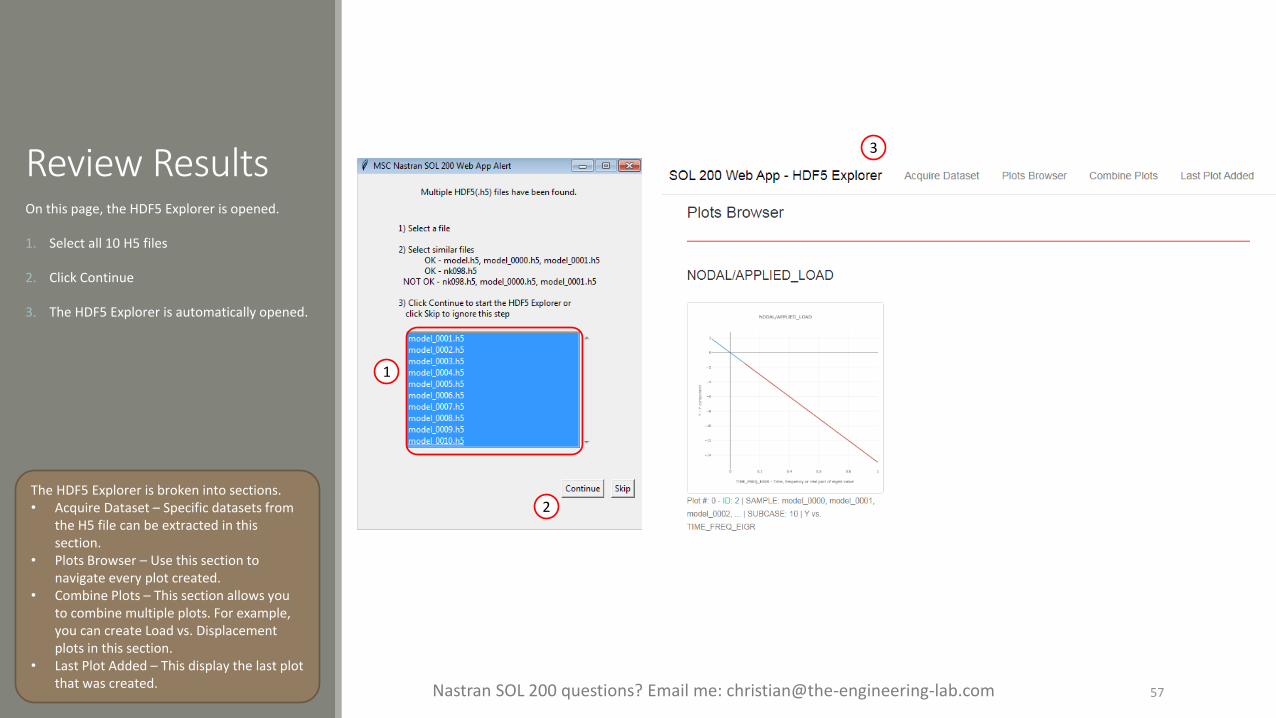
Review ResultsOn this page, the HDF5 Explorer is opened.

1. Select all 10 H5 files

2. Click Continue

3. The HDF5 Explorer is automatically opened.

The HDF5 Explorer is broken into sections.• Acquire Dataset – Specific datasets from

the H5 file can be extracted in this section.

• Plots Browser – Use this section to navigate every plot created.

• Combine Plots – This section allows you to combine multiple plots. For example, you can create Load vs. Displacement plots in this section.

• Last Plot Added – This display the last plot that was created.

3

1

2


Review Results1. Click Combine Plots

2. For Dataset A, Plot Number, select 0

3. For Dataset B, Plot Number, select 1

4. Click Update Plot

5. Mark both checkboxes

6. Click Display None

7. Mark the checkbox for the first 4 samples

8. The corresponding load vs. displacement plot is created

1

2

3

5

4

6

7

8


End of Tutorial


Appendix


Appendix Contents◦ How to import and edit previous files

◦ What is Gaussian Process Regression?


How to import and edit previous files


How to import and edit previous filesThe parameters, samples and responses are contained in the following files

◦ app.config

◦ BDF files

These files may be imported back to the Parameter Study web app, and any parameters, samples and responses can be reconfigured


• Refreshing the page is only required when the Select files button is disabled.

Import1. Return to the window or tab that has the

Parameter Study web app opened

2. Refresh the web page to start a new session

1

2


1

5

• All imports require the app.config file to be selected.

Import1. Click Select Files

2. Navigate to the folder named nastran_working_directory

3. Select all the BDF files AND the app.configfile.

4. Click Open


3

4

2


ImportFor the Response section, the H5 file will need to be re-uploaded.

1. Click Responses

2. Select the H5 file

3. Click Upload

4. Data from the H5 is loaded and ready to use

2

3

4

1


ImportAfter import, any Parameter, Samples or Responses can be modified.


What is Gaussian Process Regression?


MVN Conditioning Equations Training Data

𝐷𝑛: Training data 𝑋𝑛(inputs) and 𝑌𝑛 (outputs)

Gaussian Process Regression Overview

Covariance Function (Kernel)*

𝛴 𝑥, 𝑥′ = 𝑘(𝑥, 𝑥′)

Prediction Uncertainty

Variance: 𝛴 𝑥 or σ2 𝑥

Predicted Values(Surrogate Model)

Mean: 𝜇 𝑥

* Hyperparameter optimization is part of the procedure but not covered in this presentation


Multivariate Normal (MVN) Conditioning EquationsThe following must be calculated: Covariance Matrix, Mean and Variance

Covariance Matrix Σ =)Σ(𝜒, 𝜒 )Σ(𝜒, 𝑋𝑛)Σ(𝑋𝑛, 𝜒 )Σ𝑛 = Σ(𝑋𝑛, 𝑋𝑛

Apply the covariance function 𝛴 𝑥, 𝑥′ (kernel 𝑘(𝑥, 𝑥′))• )Σ(𝜒, 𝜒 : Covariance between testing (predictive) locations and themselves• )Σ(𝜒, 𝑋𝑛 : Covariance between testing (predictive) and training locations• )Σ(𝜒, 𝑋𝑛 : Covariance between training and testing (predictive) locations,

which is the transpose of )Σ(𝜒, 𝑋𝑛• )Σ𝑛 = Σ(𝑋𝑛, 𝑋𝑛 : Covariance between training locations and themselves

MVN Conditioning Equations (Mean and Variance)Also referred to as “Gaussian process regression,” “kriging” or “kriging equations”

Predicted values


𝑋𝑛: Training locations𝜒: Testing (predictive) locations


Example 1


Example 1Suppose a black box function was executed at 4 different samples (x1, x2 combinations)

With limited data (x and y), what does the response surface look like?

Sample x1 x2 y

1 -1.03 1.76 −1.56𝑒−02

2 .49 .49 3.04𝑒−01

3 1.77 -1.77 3.38𝑒−03

4 3.62 3.76 5.43𝑒−12

Training Data


Training Data and Testing (Predictive) LocationsSuppose you have the following training data and testing locations

◦ 𝑋𝑛 : The training design consists of 4 points

◦ 𝜒 : The test design (locations to make predictions) consists of 2 points

Where,

◦ 𝑋𝑛: inputs of the training data

◦ 𝑌𝑛: outputs of the training data

◦ 𝜒: inputs of the testing data (predictive locations, i.e. points to make predictions)

◦ 𝑦 ∗: predicted outputs

◦ 𝐷𝑛: Training data 𝑋𝑛 and 𝑌𝑛

The goal is make predictions (𝑦 ∗) for points in 𝜒

𝑋 =𝜒𝑋𝑛

=

.35 .69

.65 .46−1.03 1.76.49 .491.77 −1.773.62 3.76

𝑦 ∗𝑌𝑛

= −1.56𝑒 − 023.04𝑒 − 013.38𝑒 − 035.43𝑒 − 12

??


Calculation of the Covariance Matrix1. Select a covariance (kernel) function

◦ Many covariance functions (kernels) exist: Radial Basis Function (RBF), Matern 5/2, 3/2, Exponential, …

◦ For this example, a form of the RBF covariance function is used. This covariance function is described as the “inverse exponentiated squared Euclidean distance”

2. Calculate 𝐷 (Distance Matrix)

3. Calculate 𝛴 (Covariance Matrix)

𝐷 = 𝑋 − 𝑋 2

𝛴 = 𝑒−𝐷

= 𝑒− 𝑥−𝑥′2

“Norm between 𝑋 and 𝑋, squared”

𝑘(𝑥, 𝑥′) =


.35 − .35 2 + .69 − .69 22

= 0.35 − .65 2 + .69 − .46 2

2

= .1429.35 − −1.03 2 + .69 − 1.76 2

2

= 3.0493

.35 − .49 2 + .69 − .49 22

= .0596.35 − 1.77 2 + .69 − −1.77 2

2

= 8.068.35 − 3.62 2 + .69 − 3.76 2

2

= 20.1178

.1429 .65 − .65 2 + .46 − .46 22

= 0.65 − −1.03 2 + .46 − 1.76 2

2

= 4.5124

.65 − .49 2 + .46 − .49 22

= .0265

.65 − 1.77 2 + .46 − −1.77 22

= 6.2273.65 − 3.62 2 + .46 − 3.76 2

2

= 19.7109

3.0493 4.5124 −1.03 − −1.03 2 + 1.76 − 1.76 22

= 0

−1.03 − .49 2 + 1.76 − .49 22

= 3.9233

−1.03 − 1.77 2 + 1.76 − −1.77 22

=20.3009−1.03 − 3.62 2 + 1.76 − 3.76 2

2

=25.6225

.0596 .0265 3.9233.49 − .49 2 + .49 − .49 2

2

= 0

.49 − 1.77 2 + .49 − −1.77 22

= 6.746.49 − 3.62 2 + .49 − 3.76 2

2

= 20.4898

8.068 6.2273 20.3009 6.746 1.77 − 1.77 2 + −1.77 − −1.77 22

= 01.77 − 3.62 2 + −1.77 − 3.76 2

2

= 34.0034

20.1178 19.7109 25.6225 20.4898 34.00343.62 − 3.62 2 + 3.76 − 3.76 2

2

= 0

Calculation of 𝐷

𝐷 =


𝑒0 = 1 𝑒−.1429 = .8668 𝑒−3.0493 = .0474 𝑒−.0596 = .9421 𝑒−8.068 = .0003 𝑒−20.1178 = 1.832e-9

.8668 𝑒0 = 1 𝑒−4.5124 =.0110 𝑒−.0265 = .9738 𝑒−6.2273 =.0020 𝑒−19.7109 =2.8e-9

.0474 .0110 𝑒0 = 1 𝑒−3.9233 = .0198 𝑒−20.3009 = 1.5e-9 𝑒−25.6225 = 7.5e−12

.9421 .9738 .0198 𝑒0 = 1 𝑒−6.746 = .0012 𝑒−20.4898 = 1.263e-9

.0003 .0020 1.5e-9 .0012 𝑒0 = 1 𝑒−34.0034 = 1.7e−15

1.832e-9 2.8e-9 7.5e−12 1.263e-9 1.7e−15 𝑒0 = 1

Calculation of 𝛴

𝛴 =


𝑒0 = 1 𝑒−.1429 = .8668 𝑒−3.0493 = .0474 𝑒−.0596 = .9421 𝑒−8.068 = .0003 𝑒−20.1178 = 1.832e-9

.8668 𝑒0 = 1 𝑒−4.5124 =.0110 𝑒−.0265 = .9738 𝑒−6.2273 =.0020 𝑒−19.7109 =2.8e-9

.0474 .0110 𝑒0 = 1 𝑒−3.9233 = .0198 𝑒−20.3009 = 1.5e-9 𝑒−25.6225 = 7.5e−12

.9421 .9738 .0198 𝑒0 = 1 𝑒−6.746 = .0012 𝑒−20.4898 = 1.263e-9

.0003 .0020 1.5e-9 .0012 𝑒0 = 1 𝑒−34.0034 = 1.7e−15

1.832e-9 2.8e-9 7.5e−12 1.263e-9 1.7e−15 𝑒0 = 1

Calculation of 𝛴

𝛴 =

)Σ(𝜒, 𝜒 )Σ(𝜒, 𝑋𝑛

)Σ(𝑋𝑛, 𝜒 )Σ𝑛 = Σ(𝑋𝑛, 𝑋𝑛

Since 𝛴 is symmetric, note that )Σ(𝑋𝑛, 𝜒 = )Σ(𝜒, 𝑋𝑛T


Calculation of Predictive QuantitiesThe MVN conditioning equations are used to determine the predictive quantities mean and variance

Predicted values for locations in 𝜒𝜇 𝜒 = 𝑦 ∗=0.28496570.2954011

Σ 𝜒 =0.11154162 −0.05042265−0.05042265 0.05155061

This is used to compute the prediction interval

The diagonal terms are the variances at prediction points 1 and 20.111541620.05155061



RCode to replicate this example in Rlibrary(plgp)

eps = sqrt(.Machine$double.eps)

# Training points

X = rbind(c(-1.03,1.76), c(.49,.49), c(1.77,-1.77), c(3.62,3.76))

# The goal is to fit this function: y(x) = x1 * exp(-x1^2 - x2^2)

y = X[,1] * exp(-X[,1]^2 - X[,2]^2)

# Test points

XX = rbind(c(.35, .69),c(.65, .46))

XX

# Sigma 22 (Sigma) and its inverse (Si)

# ################################################

# Distance among the Training Data

D = distance(X)

Sigma = exp(-D)

Si = solve(Sigma)

# Sigma 11

# ################################################

# Distance among the Testing Data

DXX = distance(XX)

SXX = exp(-DXX)

# Sigma 12 and Sigma 21 (Transpose of Sigma 12)

# ################################################

# Distance between training and testing data

DX = distance(XX, X)

SX = exp(-DX)

# Calculate the predictive mean and predictive variance

# ################################################

# Predictive mean

mup = SX %*% Si %*% y

mup

# Predictive variance

Sigmap = SXX - SX %*% Si %*% t(SX)

Sigmap

Output

Mean

Variance


RCode to replicate this example in R with Plotslibrary(plgp)

library(lhs)


# Training Data

# ################################################

# Training points

number_of_sample_points = 4

X = rbind(c(-1.03,1.76), c(.49,.49), c(1.77,-1.77), c(3.62,3.76))

# Observed values


y = X[,1] * exp(-X[,1]^2 - X[,2]^2)

# Testing Data

# ################################################

# Test points

number_of_test_points_per_axis = 40

xx = seq(-2, 4, length=number_of_test_points_per_axis)

XX = expand.grid(xx, xx)


# ################################################


D = distance(X)

Sigma = exp(-D) + diag(eps, nrow(X))

Si = solve(Sigma)

# Sigma 11

# ################################################


DXX = distance(XX)

SXX = exp(-DXX)


# ################################################



SX = exp(-DX)


# ################################################

mup = SX %*% Si %*% y


# Predictive standard deviation

diag(Sigmap)

sdp = sqrt(diag(Sigmap))

# Figure 5.5

par(mfrow=c(1, 2))

cols_a = hcl.colors(128, palette = "viridis")

cols_b = heat.colors(128)

image(xx, xx, matrix(mup, ncol=length(xx)), xlab='x1', ylab='x2', col=cols_a)

points(X[,1], X[,2])

image(xx, xx, matrix(sdp, ncol=length(xx)), xlab='x1', ylab='x2', col=cols_b)


# Figure 5.6

persp(xx, xx, matrix(mup, ncol=number_of_test_points_per_axis), theta=-30, phi=30,

xlab='x1', ylab='x2', zlab='y', zlim = c(-.5,.5))


Predictive Quantities Mean and Standard Deviation

Mean: 𝜇 𝜒Standard Deviation

(Square root of variances (Diagonals of Σ 𝜒 )

Not Good – High Standard Deviation – High Variance – High Prediction uncertainty (Prediction is not reliable)

Good – Low Standard Deviation – Low Variance – Low Prediction uncertainty (Prediction is reliable)

Prediction uncertainty is lowest near training data locations


Comparison of True and Predicted FunctionsTrue Function Predicted Function (𝜇 𝜒 )

Source: https://www.sfu.ca/~ssurjano/grlee08.html


Example 2


Example 1 Example 2 True Function

𝑋𝑛 : The training design

4 Points 40 Points

Example 2

Predicted Function (𝜇 𝜒 )40 Training Points

True Function (𝑓 𝑥 )Predicted Function (𝜇 𝜒 )4 Training Points


RCode to replicate this example in R with more training datalibrary(plgp)

library(lhs)


# Training Data

# ################################################

# Training points

number_of_sample_points = 40

X = randomLHS(number_of_sample_points, 2)

X[,1] = (X[,1] - .5) * 6 + 1

X[,2] = (X[,2] - .5) * 6 + 1

# Observed values


y = X[,1] * exp(-X[,1]^2 - X[,2]^2)

# Testing Data

# ################################################

# Test points

number_of_test_points_per_axis = 40

xx = seq(-2, 4, length=number_of_test_points_per_axis)

XX = expand.grid(xx, xx)


# ################################################


D = distance(X)

Sigma = exp(-D) + diag(eps, nrow(X))

Si = solve(Sigma)

# Sigma 11

# ################################################


DXX = distance(XX)

SXX = exp(-DXX)


# ################################################



SX = exp(-DX)


# ################################################

mup = SX %*% Si %*% y


# Predictive standard deviation

diag(Sigmap)

sdp = sqrt(diag(Sigmap))

# Figure 5.5

par(mfrow=c(1, 2))

cols_a = hcl.colors(128, palette = "viridis")

cols_b = heat.colors(128)

image(xx, xx, matrix(mup, ncol=length(xx)), xlab='x1', ylab='x2', col=cols_a)


image(xx, xx, matrix(sdp, ncol=length(xx)), xlab='x1', ylab='x2', col=cols_b)


# Figure 5.6

persp(xx, xx, matrix(mup, ncol=number_of_test_points_per_axis), theta=-30, phi=30,

xlab='x1', ylab='x2', zlab='y', zlim = c(-.5,.5))


Predictive Quantities Mean and Standard Deviation

Mean: 𝜇 𝜒Standard Deviation

(Square root of variances (Diagonals of Σ 𝜒 )

Not Good – High Standard Deviation – High Variance – High Prediction uncertainty (Prediction is not reliable)

Good – Low Standard Deviation – Low Variance – Low Prediction uncertainty (Prediction is reliable)

Prediction uncertainty is lowest near training data locations


Comparison of True and Predicted FunctionsTrue Function Predicted Function (𝜇 𝜒 )

Source: https://www.sfu.ca/~ssurjano/grlee08.html

workshop prediction analysis, post ... - the engineering lab

Documents