worldwide evidence of a unimodal relationship between

1

Worldwide Evidence of a Unimodal Relationship Between Productivity and

Plant Species Richness

Lauchlan H. Fraser1*, Jason Pither

2, Anke Jentsch

3, Marcelo Sternberg

4, Martin Zobel

5, Diana

Askarizadeh6, Sandor Bartha

7, Carl Beierkuhnlein

8, Jonathan A. Bennett

9, Alex Bittel

10,

Bazartseren Boldgiv11

, Ilsi I. Boldrini12

, Edward Bork13

, Leslie Brown14

, Marcelo Cabido15

,

James Cahill9, Cameron N. Carlyle

13, Giandiego Campetella

16, Stefano Chelli

16, Ofer Cohen

4,

Anna-Maria Csergo17

, Sandra Díaz15

, Lucas Enrico15

, David Ensing2, Alessandra Fidelis

18, Jason

D. Fridley19

, Bryan Foster10

, Heath Garris20

, Jacob R. Goheen21

, Hugh A.L. Henry22

, Maria

Hohn23

, Mohammad Hassan Jouri24

, John Klironomos2, Kadri Koorem

5, Rachael Lawrence-

Lodge25

, Ruijun Long26

, Pete Manning27

, Randall Mitchell20

, Mari Moora5, Sandra C. Müller

28,

Carlos Nabinger29

, Kamal Naseri30

, Gerhard E. Overbeck12

, Todd M. Palmer31

, Sheena

Parsons10

, Mari Pesek10

, Valério D. Pillar28

, Robert M. Pringle32

, Kathy Roccaforte10

, Amanda

Schmidt1, Zhanhuan Shang

26, Reinhold Stahlmann

8, Gisela C. Stotz

9, Shu-ichi Sugiyama

33,

Szilárd Szentes34

, Don Thompson35

, Radnaakhand Tungalag11

, Sainbileg Undrakhbold11

,

Margaretha van Rooyen36

, Camilla Wellstein37

, J. Bastow Wilson25,38

, Talita Zupo18

.

Affiliations: 1Department of Natural Resource Sciences, Thompson Rivers University, Kamloops, BC,

Canada.

2Department of Biology, University of British Columbia, Okanagan campus, Kelowna, BC,

Canada.

3Department of Disturbance Ecology, BayCEER, University of Bayreuth, Bayreuth, Germany.

4Department of Molecular Biology & Ecology of Plants, Tel Aviv University, Tel-Aviv, Israel.

5Department of Botany, Institute of Ecology and Earth Sciences, University of Tartu, Tartu,

Estonia.

6Faculty of Natural Resources College of Agriculture & Natural Resources, University of

Tehran, Iran.

7MTA Centre for Ecological Research, Institute of Ecology and Botany, Vácrátót, Hungary and

School of Plant Biology, The University of Western Australia, Crawley Australia.

8Department of Biogeography, BayCEER, University of Bayreuth, Germany.

9Department of Biological Sciences, University of Alberta, AB, Canada.

10

Department of Ecology and Evolutionary Biology, University of Kansas, KS, USA.

11

Department of Biology, National University of Mongolia, Ulaanbaatar, Mongolia

2

12Department of Botany, Universidade Federal do Rio Grande do Sul, Porto Alegre, Brazil.

13

Department of Agricultural, Food and Nutritional Sciences, University of Alberta, AB, Canada.

14

Applied Behavioural Ecology & Ecosystem Research Unit, University of South Africa, South

Africa.

15

Instituto Multidisciplinario de Biología Vegetal (IMBIV-CONICET) and Facultad de Ciencias

Exactas, Físicas y Naturales, Universidad Nacional de Córdoba

16

School of Biosciences and Veterinary Medicine, University of Camerino, Camerino, Italy.

17

School of Natural Sciences, Trinity College Dublin, Dublin, Ireland.

18

Departamento de Botânica, UNESP - Univ. Estadual Paulista, Rio Claro, Brazil.

19

Department of Biology, Syracuse University, Syracuse, NY USA.

20Department of Biology, University of Akron, OH, USA

21

Department of Zoology and Physiology, University of Wyoming, Laramie, WY, USA.

22

Department of Biology, University of Western Ontario, London, ON, Canada.

23

Department of Botany, Corvinus University of Budapest, Budapest, Hungary.

24

Department of Natural Resources, Islamic Azad University, Nour Branch, Iran.

25

Department of Botany, University of Otago, Dunedin, New Zealand

26

International Centre for Tibetan Plateau Ecosystem Management, Lanzhou University, China.

27

Institute of Plant Sciences, University of Bern, Altenbergrain 21, CH-3013, Bern, Switzerland.

28

Department of Ecology, Universidade Federal do Rio Grande do Sul, Porto Alegre, Brazil.

29

Faculty of Agronomy, Universidade Federal do Rio Grande do Sul, Porto Alegre, Brazil.

30

Department of Range and Watershed Management, Ferdowsi University of Mashhad, Iran.

31

Department of Biology, University of Florida, Gainesville, FL, USA.

32

Department of Ecology & Evolutionary Biology, Princeton University, Princeton, NJ, USA.

33

Laboratory of Plant Ecology, Hirosaki University, Hirosaki, Japan.

3

34Institute of Plant Production, Szent István University, Gödöllő, Hungary.

35

Agriculture and Agri-Food Canada, Lethbridge Research Centre, Lethbridge, AB, Canada.

36

Department of Plant Science, University of Pretoria, Pretoria, South Africa.

37

Faculty of Science and Technology, Free University of Bozen-Bolzano, Bolzano, Italy

38

Landcare Research, Dunedin, New Zealand.

*Corresponding author. Email: [email protected]

One Sentence Summary: Empirical evidence from grasslands around the world shows a

humped-back relationship between biomass production and plant species richness.

Abstract: The search for predictions of species diversity across environmental gradients

has challenged ecologists for decades. The humped-back model (HBM) suggests that plant

diversity peaks at intermediate productivity; at low productivity few species can tolerate

the environmental stresses and at high productivity a few highly competitive species

dominate. Over time the HBM has become increasingly controversial, and recent studies

claim to have refuted it. Here, using data from coordinated surveys conducted throughout

grasslands worldwide, and comprising a wide range of site productivities, we provide

strong evidence in support of the HBM pattern, at both global and regional extents. The

relationships described here provide a strong foundation for further research into the local,

landscape, and historical factors that ensure the maintenance of biodiversity.

Main Text: Despite a long history of research, the nature of basic patterns between

environmental factors and biological diversity remain poorly defined. A notable example is the

mailto:[email protected]

4

relationship between plant diversity and productivity, which has stimulated a long-running

debate (1-6). A classic hypothesis, the humped-back model (HBM) (7), states that plant species

richness peaks at intermediate productivity, taking above-ground biomass as a proxy for annual

net primary productivity (7-9). This diversity peak is driven by two opposing processes. In

unproductive ecosystems with low plant biomass, species richness is limited by abiotic stress,

such as insufficient water and mineral nutrients, which few species are able to tolerate. In

contrast, in the productive conditions that generate high plant biomass, competitive exclusion by

a small number of highly competitive species is hypothesized to constrain species richness (7-9).

Other mechanisms that may explain the unimodal relationship between species richness and

biomass include disturbance (7, 10), evolutionary history and dispersal limitation (11, 12), and

the reduction of total plant density in productive communities (13).

Since its initial proposal a range of studies have both supported and rejected the HBM, and three

separate meta-analyses reached different conclusions (14-17). While this inconsistency may

indicate a lack of generality of the HBM, it may instead reflect a sensitivity to study

methodology, including the plant community types considered, the taxonomic scope, the range

of site productivities sampled, the spatial grain and extent of analyses (17, 18), and the particular

measure of net primary productivity used (19). The question therefore remains open as to what

the form of the relationship between diversity and productivity is, and whether the HBM serves

as a useful and general model for grassland ecosystem theory and management.

We quantified the form and strength of the richness-productivity relationship using globally

coordinated surveys (20), which yielded scale-standardized data, and were distributed across 30

5

sites in 19 countries and 6 continents (Fig. 1). Collectively, our samples spanned a broad range

of biomass production (from 2 to 5,711 g m-2

) and grassland community types, including natural

and managed (pastures, meadows) grasslands over a wide range of climatic zones (temperate,

Mediterranean and tropical), and altitudes (lowland to alpine) (table S1). Our protocol involved

sampling sixty-four 1 m2 quadrats within 8 m x 8 m grids (18, 21). At each site, between two and

14 grids were sampled, thus resulting in 128 – 896 quadrats per site. In each 1 m2 quadrat, we

identified and counted all plant species, and harvested above-ground biomass and plant litter.

Litter production is a function of annual net primary productivity in grasslands and can have

profound effects on the structure and functioning of communities, from altering nutrient cycling

to impeding vegetative growth and seedling recruitment (22, 23), thereby also playing a major

role in driving community structure. Indeed, the HBM was originally defined in terms of live

biomass plus litter material (7, 8). Most of the sites in our survey were subject to some form of

management, usually livestock grazing or mowing. In this respect, our sites are representative of

most of the world’s grasslands. Our sampling was conducted at least three months after the last

grazing, mowing or burning event, and at the annual peak of live biomass, which, when coupled

with litter constitutes a reliable measure of annual net aboveground production in herbaceous

plant communities (24).

Our results strongly support the humped-back model of the plant richness-productivity

relationship. Using a global-extent regression model (N = 9631 1 m2 quadrats; 21) we found that

plant richness formed a unimodal relationship with productivity (Fig. 2A), that is characterized

by a highly significant concave-down quadratic regression (negative binomial generalized linear

model; Table 1). This relationship was not sensitive to the statistical model used; the hump-

6

backed relationship was also evident when we used a negative binomial generalized linear mixed

model (GLMM) that accommodated the hierarchical structure of our sampling design (grids

nested within sites; Table 1 and fig. S1).

At a sampling grain of 1 m2, 19 of 28 site level analyses (68%) yielded significant concave-down

relationships (table S2 and Fig. 2A). This contrasts markedly with the results of Adler et al. (1),

who found only 1 of their 48 within-site analyses to be significantly concave-down. We also

found the form of the productivity-diversity relationship to be robust to sampling grain: using

grains of 1 m2 up to 64 m

2, each time maintaining a global extent, we consistently found a

significant concave-down relationship, though the proportion variation explained tended to

decrease with increasing grain (fig. S2).

The HBM predicts a boundary condition or upper limit to diversity that, in any given site, may

not be realized for a variety of reasons (18). Consistent with this view, our global-extent

association is characterized by a significant concave-down quantile regression (95th

percentile)

(Table 1), below which considerable scatter exists (Fig. 2A). This pattern was also insensitive to

the statistical method used; a hierarchical Bayesian analysis that accommodated the nested

sampling design, and that enabled both the mean and the variance of species richness to be

modeled more accurately against (log-transformed) biomass, also revealed a significant 95th

percentile quantile regression (fig. S3). Likewise, we found a significant, concave-down quantile

regression (95th

percentile) between the maximum (quadrat-scale) richness found within a grid

and the total biomass of the same quadrat (Table 1; fig. S4). Each of these approaches to

characterizing boundary conditions suggests the existence of a “forbidden space”, wherein high

7

productivity precludes high local diversity. Furthermore, they suggest that extremely low -

productivity sites rarely accommodate high diversity.

Why do our data show a hump-backed relationship while those of Adler et al. (1), or related

studies (4, 6), do not? One possibility is that data limitations can thwart detection of the HBM

(18). For example, the data used by Adler et al. differed from ours in the following potentially

important ways: (i) they exhibited a maximum live biomass of only 1,535 gm-2

(ours was 3,374

gm-2

) (ii) litter was not included within the calculation of biomass, and (iii) sample size was

limited to 30 quadrats per site (ours ranged from 128 to 894 quadrats per site; table S1). We

conducted a form of sensitivity analysis in which we re-ran our statistical analyses using random

subsets of our data that were constrained to exhibit similar properties to those of the Adler et al.

dataset. Specifically, after limiting the overall dataset to less than 1,535 gm-2

and excluding litter,

we randomly selected 30 quadrats per site 500 times, each time conducting the within-site

regression analyses (N = 30 for each of the 28 site-level GLMs conducted per subsampling

iteration). For each iteration, we also calculated the average range of biomass spanned by the 28

site-level relationships. Across the 500 iterations (one example set of outcomes shown in Fig.

2B), the average proportion of significant concave-down, within-site regressions was 0.31

0.003 (SEM), significantly less than our observed proportion of 0.68 (fig. S5). Moreover, when

significant concave-down relationships were detected, they tended to span a broader range of

biomass than the remaining forms (including non-significant relationships). Specifically, in 458

of the 500 iterations (92%), the mean biomass range of the concave-down regressions was larger

than the mean of the remaining forms’ biomass ranges (Binomial test: P < 2.2 x 10-16

). Finally,

the 48 within-site analyses of Adler et al. spanned, on average, a live biomass range of 428.7gm-2

8

38.36 (range: 89 – 1217 gm-2

). This is (i) less than half of the average range encompassed by

our 28 site-level analyses shown in Fig. 2A (mean = 1,067.5 gm-2

140.63; range 286 to 3,256

gm-2

), and (ii) almost 50% narrower than the smallest average biomass range encompassed by

our 500 random subset analyses (627.4 gm-2

) (fig. S6). Taken together, these findings strongly

suggest that we were able to detect more concave-down relationships because of the greater

sample sizes and biomass ranges in our analysis.

It has been suggested (2) that some previous studies, including Adler et al (1), failed to support

the HBM because they excluded litter. Although we do find a significant concave-down

relationship at the global extent using only live biomass (Table 1), a comparison of models using

biomass versus biomass+litter (both N = 9,631) shows total biomass to provide a far better fit

(residual deviance = 10,105 (live) versus 10,037 (total); Vuong z-statistic for comparing non-

nested models: -13.4; P < 0.001). It has also been suggested that previous surveys failed to

adequately represent high-productivity communities. Indeed, our high-biomass quadrats (1,011

samples were over 1,000 gm-2

, approximately 10% of the 9,631 samples; maximum 5,711 gm-2

),

contributed considerably to the right-hand part of the fitted humped-back regression. This could

be a reason why the dataset of Adler et al. (1) (in which only 0.5% of samples were over 1,000

gm-2

and a maximum of 1,534 gm-2

) failed to support the HBM. Our results therefore show that a

test of the HBM in herbaceous plant communities yields the expected pattern when it is robust

and comprehensive; spans a wide range of biomass production (from 1 to at least 3,000 dry gm-2

yr-1

), and provides sufficient replication of quadrats along the productivity gradient.

9

Competitive exclusion has been cited as the primary factor driving low species numbers at high

plant biomass (7, 8, 25). However, in the case of nitrogen addition the negative relationship

between productivity and species richness has been shown to diminish over time (26 but see 27,

28). It may be that low species richness in high-productivity conditions arises in part because

most such habitats are anthropogenic, and there are few species in the local pool adapted to these

conditions (11, 12). If so, it is possible that species will eventually immigrate from distant pools,

so that the right-hand part of the hump will then flatten out.

We have shown a global-scale concave-down unimodal relationship between biomass production

and richness in herbaceous grassland communities. However, the original HBM (7) is vaguely

articulated by the standards of modern ecological theory and it is clear that more work is needed

to determine the underlying causal mechanisms that drive the unimodal pattern (1, 6, 17, 18). We

recognize that in our study and many others productivity accounts for a fairly low proportion of

the overall variation in richness, and that many other drivers of species richness exist (28, 29).

Accordingly, we echo the call of Adler et al. (1) for additional efforts to understand the

multivariate drivers of species richness.

REFERENCES AND NOTES

1. P. B. Adler et al. Productivity is a poor predictor of plant species richness. Science 333, 1750-

1753 (2011).

2. J. D. Fridley et al. Comment on “Productivity is a poor predictor of plant species richness”

Science 335, 1441 (2012).

10

3. X. Pan, F. Liu, M. Zhang. Comment on “Productivity is a poor predictor of plant species

richness”. Science 335, 1441 (2012).

4. Grace, J. B. et al. Response to comments on “Productivity is a poor predictor of plant species

richness”. Science 335, 1441 (2012).

5. S. Pierce. Implications for biodiversity conservation of the lack of consensus regarding the

humped-back model of species richness and biomass production. Funct. Ecol. 28, 253-257

(2014).

6. J. B. Grace, P. B. Adler, W. S. Harpole, E. T. Borer, E. W. Seabloom. Causal networks clarify

productivity-richness interrelations, bivariate plots do not. Funct. Ecol. 28, 787-798 (2014).

7. J. P. Grime. Control of species density in herbaceous vegetation. J. Envir. Man. 1, 151-167

(1973).

8. M. M. Al-Mufti, C. L. Sydes, S. B. Furness, J. P. Grime, S. R. Band. A quantitative analysis of

shoot phenology and dominance in herbaceous vegetation. J. Ecol. 65, 759-791 (1977).

9. Q. Guo, W. L. Berry. Species richness and biomass: dissection of the hump-shaped

relationships. Ecology 79, 2555-2559 (1998).

10. J. H. Connell. Diversity in tropical rain forests and coral reefs. Science 199, 1302-1310

(1978).

11. M. Zobel, M. Pärtel. What determines the relationship between plant diversity and habitat

productivity? Global Ecol. Biogeogr. 17, 679-684 (2008).

12. D. R. Taylor, L. W. Aarssen, C. Loehle. On the relationship between r/K selection and

environmental carrying capacity: a new habitat templet for plant life history strategies. Oikos

58, 239-250 (1990).

11

13. J. Oksanen. Is the humped relation between species richness and biomass an artefact due to

plot size? J. Ecol. 84, 293-295 (1996).

14. G. G. Mittelbach et al. What is the observed relationship between species richness and

productivity? Ecology 82, 2381-2396 (2001).

15. L. N. Gillman, S. D. Wright. The influence of productivity on the species richness of plants:

a critical assessment. Ecology 87, 1234-1243 (2006).

16. M. Pärtel, L. Laanisto, M. Zobel. Contrasting plant productivity-diversity relationships across

latitude: the role of evolutionary history. Ecology 88, 1091-1097 (2007).

17. R. J. Whittaker. Meta-analyses and mega-mistakes: calling time on meta-analysis of the

species richness–productivity relationship. Ecology 91, 2522–2533 (2010).

18. L. H. Fraser, A. Jentsch, M. Sternberg. What drives plant species diversity? Tackling the

unimodal relationship between herbaceous species richness and productivity. J. Veg. Sci. 25,

1160-1166 (2014).

19. B. J. Cardinale, H. Hillebrand, W. S. Harpole, K. Gross, R. Ptacnik, R. Separating the

influence of resource “availability” from resource “imbalance” on productivity-diversity

relationships. Ecol. Lett. 12, 475-487 (2009).

20. L. H. Fraser et al. Coordinated distributed experiments: an emerging tool for testing global

hypotheses in ecology and environmental science. Front. Ecol. Envir. 11, 147-155 (2013).

21. Materials and methods are available as supplementary materials on Science Online.

22. A. K. Knapp, T. R. Seastedt. Detritus accumulation limits productivity of tallgrass prairie.

Bioscience 36, 662-668 (1986).

23. B. L. Foster, K. L. Gross. Species richness in a successional grassland: effects of nitrogen

enrichment and plant litter. Ecology 79, 2593-2602 (1998).

12

24. M. Oesterheld, S. J. McNaughton, in Methods in Ecosystem Science, O. E. Sala, R. B.

Jackson, H. A. Mooney, R. Howarth, Eds. (Springer-Verlag, New York, 2000), chap. 2, pp.

151-157.

25. T. K. Rajaniemi. Why does fertilization reduce plant species diversity? Testing three

competition-based hypotheses. J. Ecol. 90, 316-324 (2002).

26. F. Isbell et al. Nutrient enrichment, biodiversity loss, and consequent declines in ecosystem

productivity. Proc. Natl Acad. Sci. USA 110, 11911-11916 (2013).

27. K. N. Suding et al. Functional- and abundance-based mechansims explain diversity loss due

to N fertilization. Proc. Nat. Acad. Sci. 102, 4387-4392 (2005).

28. T. L. Dickson, Gross, K. L. Plant community responses to long-term fertilization: changes in

functional group abundance drive changes in species richness. Oecologia 173, 1513-1520

(2013).

29. P. Chesson. Mechanisms of maintenance of species diversity. Annu. Rev. Ecol. Syst. 31, 343-

366 (2000).

30. K. J. Gaston. Global patterns in biodiversity. Nature 405, 220-227 (2000).

31. R Core Team. R: A language and environment for statistical computing. R Foundation for

Statistical Computing, Vienna, Austria. URL http://www.R-project.org/. Version 3.13.

(2014).

32. C. Kleiber, A. Zeileis. Applied Econometrics with R. New York: Springer-Verlag. ISBN

978-0-387-77316-2. URL http://CRAN.R-project.org/package=AER (2008).

33. A. F. Zuur et al. Mixed effects models and extensions in ecology with R. Springer New

York, New York, NY (2009).

http://cran.r-project.org/package=AER

13

34. M. Plummer, in Proceedings of the 3rd International Workshop on Distributed Statistical

Computing, K. Hornik, F. Leisch, A. Zeileis, Eds. (Achim Zeileis, Vienna, Austria,

2003).

35. Y. –S. Su, M. Yajima. R2jags: A Package for Running JAGS from R. R package version

0.04-03. http://CRAN.R-project.org/package=R2jags (2014).

36. A. Gelman, D. B. Rubin. Inference from iterative simulation using multiple sequences.

Statistical Science 7, 457–472 (1992).

Acknowledgements: We are grateful to all of the people who helped in the collection and

processing of the samples; including Liam Alabiso-Cahill, D Ariunzaya, Mariana R Ávila, Júlio

C R Azambuja, Laura Bachinger, I Badamnyambuu, Kathy Baethke, J Batbaatar, Sandro Ballelli,

Kh Bayarkhuu, Gustavo Bertone, Vera Besnyői, Camila L Bonilha, Greg Boorman, Rafael A X

Borges, Tanner Broadbent, Roberto Canullo, Josephine Carding, Brenda Casper, Karen

Castillioni, Marco Cervellini, Grace Charles, Giovana Chiara, Elsa Cleland, Rachel Cornfoot,

Gayle Crowder, András István Csathó, László Demeter, Maike Demski, Miranda Deutschlander,

Sabina Donnelly, André L P Dresseno, S Enkhjin, O Enkhmandal, T Erdenebold, L

Erdenechimeg, B Erdenetsetseg, Jean K Fedrigo, Ana Carolina Ferreira, Zoltan Foldvari, Louise

Fourie, Bruce Fraser, Jonathan Galdi-Rosa, Elizabeth Gorgone-Barbosa, Ruth Greuel, Anaclara

Guido, Éva György, David Hall, Ali Hassan, Judit Házi, Roi Henkin, Samuel Hoffmann, Teele

Jairus, M Jankju, Ülle Jõgar, Tessa Jongbloets, Melinda Juhász, Cristiane F Jurinitz, Vahid

Rahimi Kakroudi, Alpár Kelemen, T Khandarmaa, E Khash-Erdene, Christiane Koch, Cecília

Komoly, Sam Kurukura, Pierre Liancourt, Simon Lima, Ariuntsetseg Lkhagva, M Lucrecia

Lipoma, D Lkhagvasuren, Julio Lombardi, M Eugenia Marcotti, Jennifer McPhee, Bryana

14

McWhirter, Luciana Menezes, Justine McCulloch, M Mesdaghi, István Máthé, Mario Messini,

Maia Mistral, Chandra Moffat, Mohamud Mohamed, Lutendo Mugwedi, Jeff Padgham, Priscila

Padilha, Susanne Paetz, S Pagmadulam, Greg Pec, Chiara Peconi, Gabriella Péter, Sándor Piros,

Vitor C Pistóia, Lysandra Pyle, Morgan Randall, Mariana Ninno Rissi, Rosângela G Rolim,

Mandy Ross, Tina Salarian, Sh Sandagdorj, S Sangasuren, Carlo Santinelli, Colin Scherer,

Graziela H M Silva, Mariana G Silva, Thomas Smith, Sh Solongo, Francesco Spada, Reinhold

Stahlmann, John Steel, Monika Sulyok, Alex Sywenky, Gábor Szabó, Lányi Szabules, Vickey

Tomlinson, Julien Tremblay-Gravel, Gergely Ungvari, O Urangoo, M Uuganbayar, Mariana S

Viera, Cleúsa E Vogel, Dan Wallach, Rita Wellstein, Juan I Withworth Hulse, Zita

Zimmermann. This work was supported in part by the Canada Research Chair Program,

Canadian Foundation for Innovation (CFI), and a Natural Sciences and Engineering Research

Council Discovery Grant (NSERC-DG) of Canada awarded to L.H.F., and Thompson Rivers

University; a CFI and NSERC-DG awarded to J.P.; the University of Tartu, Estonia, and a

European Regional Development Fund: Centre of Excellence FIBIR awarded to M.Z. and M.M.;

a Hungarian National Science Foundation (OTKA K 105608) awarded to S.B.; Taylor Family-

Asia Foundation Endowed Chair in Ecology and Conservation Biology and University of

Mongolia's Support for High Impact Research program awarded to B.B.; the Rangeland

Research Institute, University of Alberta, Canada; CONICET, Universidad Nacional de Córdoba,

FONCyT and the Inter-American Institute for Global Change Research (IAI, with support of the

US National Science Foundation) awarded to S.D., L.E., and M.C.; a NSERC-DG awarded to

J.C.; State Nature Reserve "Montagna di Torricchio" and University of Camerino, Italy;

Hungarian University of Transylvania, Romania; a Fundação Grupo Boticário, Brazil

(0153_2011_PR) awarded to A.F.; a NSF DEB-1021158 and DEB-0950100 awarded to B.F.;

15

UHURU: NSERC and CFI awarded to J.R.G and the University of Wyoming; an NSERC-DG

awarded to H.A.L.H.; an NSERC-DG awarded to J.K.; a National Natural Science Foundation of

China grant (No. 41171417) awarded to R.L.; Conselho Nacional de Desenvolvimento Científico

e Tecnológico (CNPq), Brazil (n. 307719/2012-0) awarded to S.M.; CNPq, Brazil (grants

403750/2012-1 and 307689/2014-0) awarded to V.P.; University of Florida and a NSF DEB

1149980 awarded to T.P.; Princeton Environmental Institute and a NSF DEB 1355122 awarded

to R.M.P.; a CONYCIT Becas-Chile Scholarship awarded to G.C.S. Data and R scripts

associated with this paper are deposited in the Dryad Repository (http://datadryad.org/).

16

Table 1. Regression results. Results of regression analyses of the relationship between productivity and species richness, measured at

a global extent and a sampling grain of 1m2 quadrat. Total biomass = live biomass + litter biomass. All linear and quadratic term

coefficients were highly significant (P < 0.001).

Productivity

measure

Type of regression Sample size Test of

model fit

Intercept

estimate

SEM

Linear term

coefficient

SEM

Quadratic term

coefficient

SEM

Total

biomass

negative binomial GLM (log-

link function)

9631 quadrats Likelihood

ratio stat.

= 1602.2

-2.52 0.235 4.69 0.186) -1.04 0.037

Total

biomass

negative binomial GLMM

(log-link function)

random effects: grid nested in

site

9631 quadrats

151 grids

28 sites

Likelihood

ratio stat.

= 114.0

0.91 0.191 1.33 0.133) -0.29 0.028

Total

biomass

quantile (95th

percentile) 9631 quadrats

pseudo-F

statistic

= 179.1

-12.9 7.159 45.6 5.833) -11.3 1.173

Live

biomass

negative binomial GLM (log-

link function)

9644 quadrats

Likelihood

ratio stat.

= 950.3

-2.03 0.212 4.27 0.178 -0.96 0.037

17

FIGURE LEGENDS

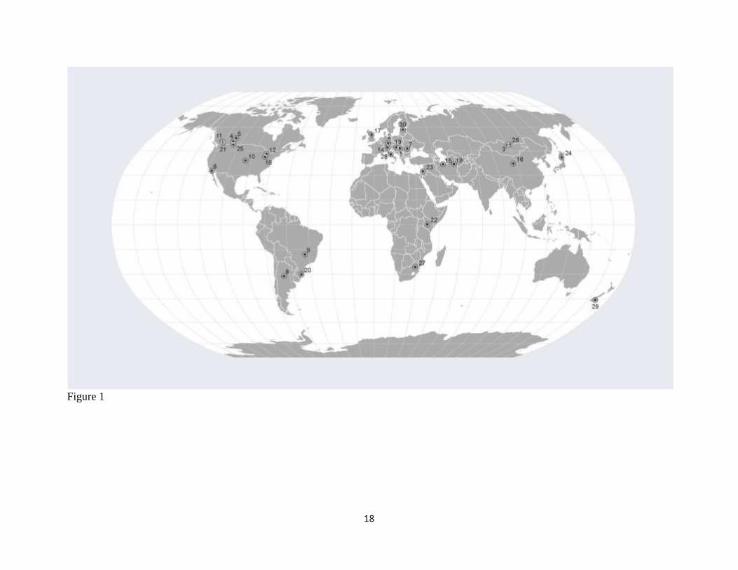
Figure 1. Site locations. Locations of the geographic centroids of the 30 study sites, which

include 151 sampling grids. Some points overlap and are therefore indistinguishable. Additional

site details are provided in table S1. Map is displayed using the Robinson projection.

Figure 2. A Biomass production-species richness relationships for 28 study sites. Solid black

line: significant quantile regression (95th

percentile) of overall relationship (quadratic coefficient

P < 0.001; N = 9,631 quadrats). Dashed black line: significant negative binomial GLM

(quadratic coefficient P < 0.001; N = 9,631). Colored lines indicate significant GLM regressions

(Poisson or quasi-Poisson), with N ranging from 128 to 894 quadrats. The inset bar graph

presents the frequencies of each form of relationship observed across study regions; B Same as A

but the results are derived from the analysis of an example, random sub-sample of the complete

dataset, that satisfies the following criteria: litter biomass excluded, quadrats with biomass

>1,534 gm-2

excluded, and including 30 (randomly selected) quadrats per site (total N = 840).

These criteria match the characteristics of the dataset used by Adler et al. (1).

18

Figure 1

Fraser et al. Productivity-diversity relationship

19

Figure 2A

5 10 20 50 100 200 500 1000 5000

0

10

20

30

40

50

Total biomass (g m-2)

Nu

mb

er

of

sp

ecie

s (m

-2)

A

NS

Lin

ea

r+

Lin

ea

r-

Co

ncave+

Conca

ve-0

5

10

15

20

Fre

que

ncy


20

Figure 2B

1 5 10 50 100 500 5000

0

10

20

30

40

50

Live biomass (g m-2)

Nu

mb

er

of

sp

ecie

s (m

-2)

B

NS

Lin

ea

r+

Lin

ea

r-

Co

ncave+

Conca

ve-0

2

4

6

8

10

12

14

Fre

qu

en

cy


21

Supplementary Materials for

Materials and Methods

Site selection: The Herbaceous Diversity Network (HerbDivNet) is a network of researchers

working at herbaceous grassland sites in 19 countries located on 6 continents performing

coordinated distributed experiments and observations (20). The full sampling design is detailed

here and in Fraser et al. (18). All HerbDivNet sites are located in areas dominated by herbaceous

vegetation representing the regional species composition.

Sampling protocol: The design is an 8 x 8 meter grid containing 64 1 m2 plots. Within all 30

sites included in the current analysis (Fig. 1) we collected biomass and species richness data

from at least two and up to fourteen 8 x 8 m grids. All grids were marked and GPS coordinates

were recorded for future use. Our study focused on herbaceous grassland community types. For

each 1 m2 plot, all species were identified and the number counted. In the rare instances where

species were unidentifiable, morphotypes were assigned. Total above-ground biomass (including

plant litter) at peak biomass was harvested, dried and weighed by plot. Live biomass and litter

were separated prior to drying and weighing. We did not separate biomass by species. Sampling

was restricted to herbaceous plant communities; however, the occasional small woody plant was

found within a sample area, which was noted but not included in the analyses. Cryptogams were

not included in either measures of species richness, or biomass.


22

The ideal level of participation for each investigator was to sample at least six grids of 64

quadrats, two each at three relatively different levels of productivity from low (~1-300 g m-2

) to

medium (~300-800 g m-2

) to high (>800 g m-2

). However, logistical constraints meant this was

not possible at all sites and some sites had as few as two grids, taken at the low and high ends of

the gradient. Most sites had a history of grazing or fire and were currently under some form of

management. Therefore, sampling was performed at least three months after the last grazing or

burning event.

Supplementary Text 1

Assessing the richness-productivity relationship at the global extent:

In the main text we present the results of generalized linear model (GLM) analysis, in which

species richness was modeled as a function of total biomass (log10 transformed) using a negative

binomial GLM. We complement this analysis with a generalized linear mixed model (GLMM)

analysis, which accommodates the spatially nested structure of our sampling design (grids nested

within sites). Regression diagnostics revealed a negative binomial distribution to be appropriate

again (as in the main GLM analyses), with grids nested within sites, both coded as random

effects, and log10-transformed total biomass as the fixed effect. This was achieved using the

“glmmADMB” package in R (31). The predicted association from this regression is shown in

Figure S1 below.


23

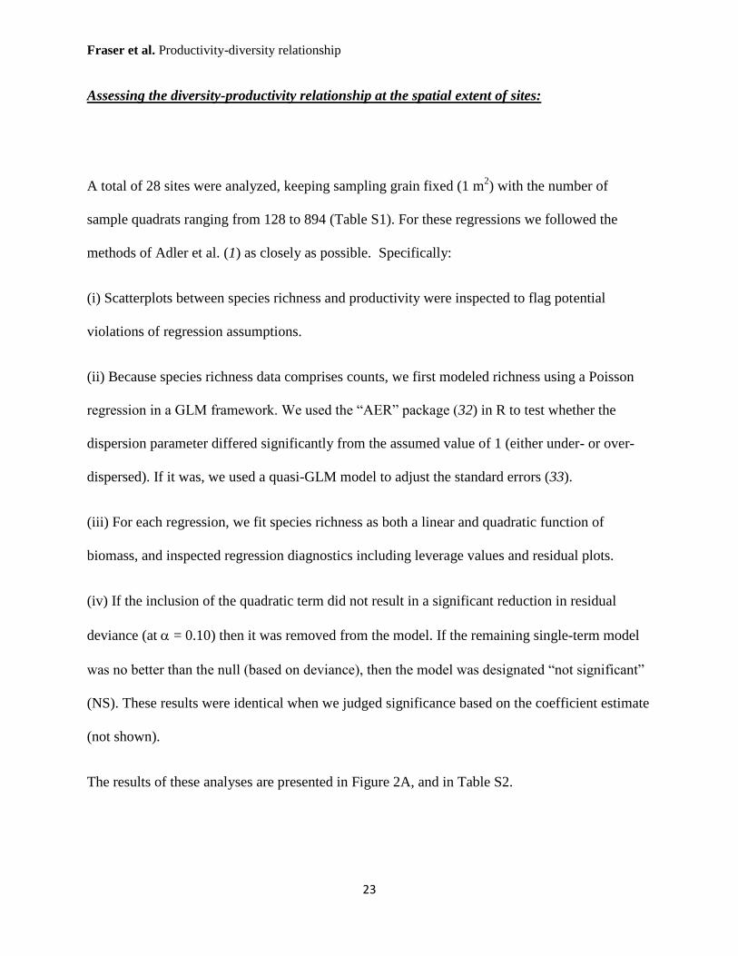
Assessing the diversity-productivity relationship at the spatial extent of sites:

A total of 28 sites were analyzed, keeping sampling grain fixed (1 m2) with the number of

sample quadrats ranging from 128 to 894 (Table S1). For these regressions we followed the

methods of Adler et al. (1) as closely as possible. Specifically:

(i) Scatterplots between species richness and productivity were inspected to flag potential

violations of regression assumptions.

(ii) Because species richness data comprises counts, we first modeled richness using a Poisson

regression in a GLM framework. We used the “AER” package (32) in R to test whether the

dispersion parameter differed significantly from the assumed value of 1 (either under- or over-

dispersed). If it was, we used a quasi-GLM model to adjust the standard errors (33).

(iii) For each regression, we fit species richness as both a linear and quadratic function of

biomass, and inspected regression diagnostics including leverage values and residual plots.

(iv) If the inclusion of the quadratic term did not result in a significant reduction in residual

deviance (at = 0.10) then it was removed from the model. If the remaining single-term model

was no better than the null (based on deviance), then the model was designated “not significant”

(NS). These results were identical when we judged significance based on the coefficient estimate

(not shown).

The results of these analyses are presented in Figure 2A, and in Table S2.


24

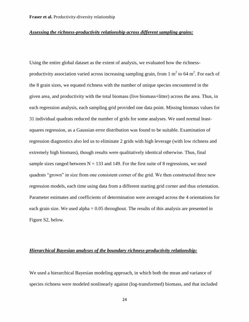
Assessing the richness-productivity relationship across different sampling grains:

Using the entire global dataset as the extent of analysis, we evaluated how the richness-

productivity association varied across increasing sampling grain, from 1 m2 to 64 m

2. For each of

the 8 grain sizes, we equated richness with the number of unique species encountered in the

given area, and productivity with the total biomass (live biomass+litter) across the area. Thus, in

each regression analysis, each sampling grid provided one data point. Missing biomass values for

31 individual quadrats reduced the number of grids for some analyses. We used normal least-

squares regression, as a Gaussian error distribution was found to be suitable. Examination of

regression diagnostics also led us to eliminate 2 grids with high leverage (with low richness and

extremely high biomass), though results were qualitatively identical otherwise. Thus, final

sample sizes ranged between N = 133 and 149. For the first suite of 8 regressions, we used

quadrats “grown” in size from one consistent corner of the grid. We then constructed three new

regression models, each time using data from a different starting grid corner and thus orientation.

Parameter estimates and coefficients of determination were averaged across the 4 orientations for

each grain size. We used alpha = 0.05 throughout. The results of this analysis are presented in

Figure S2, below.

Hierarchical Bayesian analyses of the boundary richness-productivity relationship:

We used a hierarchical Bayesian modeling approach, in which both the mean and variance of

species richness were modeled nonlinearly against (log-transformed) biomass, and that included


25

random effects to account for the nested spatial structure of the dataset. Posterior distributions

for upper quantiles (envelope) of richness were calculated from normal distributions of estimated

means and variances across the biomass gradient.

Because we expected nonlinear relationships for both the mean and variance of richness

against biomass, we included quadratic expressions for the mean and variance of richness in the

following way:

Species richnessi ~ N(µi,σ2

i)

µi = β0 + β1*Biomassi + β2*Biomassi2 + N(0,σ

2study) + N(0,σ

2grid)

σ i = α0 + α1*Biomassi + α2*Biomassi2

where the richness of quadrat i is distributed normally with mean µ and variance σ2, and mean

richness includes random intercept effects of study site and grid-within-study. To generate

posteriors for an upper quantile, we used fitted mean and variance estimates to calculate the

value of the 95th

quantile for each MCMC iteration:

q95i = qnorm(0.95,mean=µi,variance=σ2

i)

Models were fit via Markov chain Monte Carlo optimization as implemented in JAGS

(34) run from R 3.03 (31) in the R2jags package (35). We ran three parallel MCMC chains for

10,000 iterations after a 500-iteration burn-in, and evaluated model convergence with the

Gelman & Rubin statistic (36) such that chain results were indistinguishable. We used flat

normal priors for β and α coefficients, with the exception of uniform positive priors for α1 to

ensure positive variance estimates.


26

Fitted 95th

quantiles and associated 95% credible intervals for biomass including litter are

shown below (Fig. S3). Note that we did not attempt to include richness observations at

extremely low (< 50 g; 0.7% of the data) or high biomass values (> 1500 g; 3% of the data, half

of which were richness values of 1) due to low sample sizes that precluded envelope

calculations.

Assessing the boundary richness-productivity relationship using maximum grid richness as

the response, and employing quantile regression:

Using the global dataset as the extent of analysis, we quantified the upper boundary of the

richness-productivity relationship using maximum richness observed in a grid (among the 1m2

quadrats) as the response variable, and the total biomass associated with the quadrat of maximum

richness as the predictor variable. We employed quantile regression, using the 95th

percentile.

For comparison, we include the results of a least-squares regression. The results of this analysis

are presented below in Figure S4.

Examining the sensitivity of the richness-productivity relationship to biomass range, measures

of productivity, and sample size:

The goal of this suite of analyses was to mimic the properties of the dataset used by Adler et al.

(1), and to re-analyze this subset of data using the same methods employed to produce Figure

2A. The details of the subsampling procedure are described in the main document, and the


27

regression methods we used are identical to those described in section “C” above. For the GLM

analysis conducted on each of the 500 random subsets of data (see main document), we

calculated the proportion of the within-site regressions (out of 28 total) falling into each of the

five categories of form. In Figure S5 below we show how these proportions compare to our

observed proportions.

Lastly, for each iteration, we calculated the range of biomass encompassed by each site

(based on its random sample of 30 quadrats). We then calculated the average of these biomass

ranges across the 28 site-level analyses, for each iteration. Figure S6 below shows a histogram of

the resulting 500 average biomass ranges, along with the average biomass range encompassed by

the 48 site-level analyses of Adler et al. (data kindly provided by Jim Grace, and is housed at the

Nutrient Network website: http://nutnet.umn.edu/data).

http://nutnet.umn.edu/data


28

Supplementary Figures

Supplementary Figure 1: The unimodal productivity-richness relationship. Superimposed

over the individual quadrat values (light grey points; N = 9631) are the regression lines from the

negative binomial GLM (black line; see Table 1) and the negative binomial GLMM in red

(population level prediction), in which grids (N = 151) are nested within sites (N = 28), both as

random effects (Log-likelihood = -23097.9; quadratic term coefficient = -0.29, Z-value = -10.4,

P < 0.001).

2 5 10 20 50 200 500 2000

0

10

20

30

40

50

Total biomass (log10) (g m-2)

Nu

mb

er

of

sp

ecie

s (m

-2)


29


30

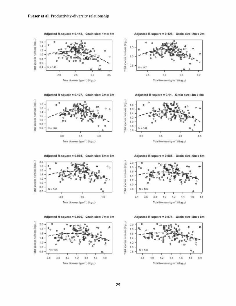
Supplementary Figure 2: Biomass-species richness relationship as it relates to scale.

Varying the sampling grain (maintaining global extent) does not change the general form of the

relationship between species richness and biomass, though the amount of variation accounted for

by the model (see adjusted R2 values) generally decreases with increasing grain. At every scale,

the quadratic term was significant (P < 0.05). Dashed lines indicate the least-squares regression.

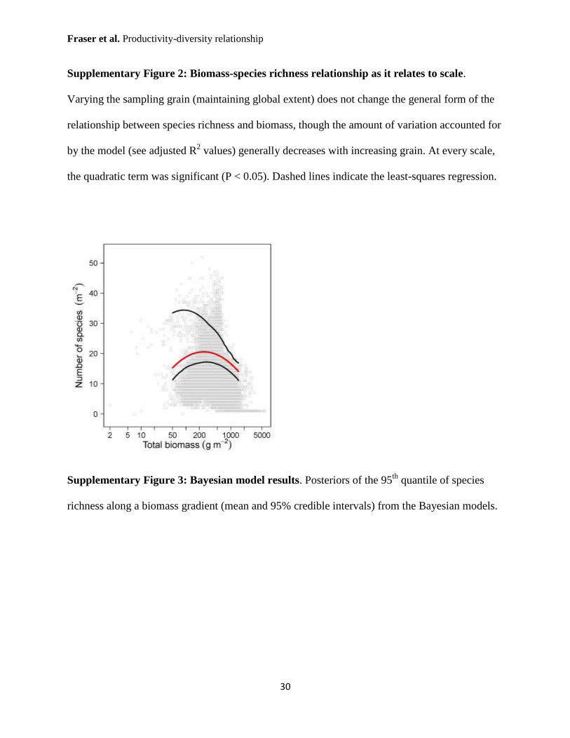
Supplementary Figure 3: Bayesian model results. Posteriors of the 95th

quantile of species

richness along a biomass gradient (mean and 95% credible intervals) from the Bayesian models.


31

Supplementary Figure 4: Estimating the upper boundary of richness in relation to

productivity. Individual points show the maximum richness observed among 1 m2 quadrats

within a grid (N = 151 grids) paired with its associated total biomass. The solid black line

represents the 95th

percentile quantile regression that determines the boundary condition

(quadratic term coefficient = -37.77, SE = 13.36, P = 0.005; pseudo R2 = 0.14). The grey line

represents the least-squares regression that includes a highly significant quadratic term (quadratic

term coefficient = -0.94, SE = 0.14, P < 0.001; adjusted R2 = 0.33). Excluding the two points

with zero richness (bottom right) did not affect the significance of the quadratic term in either

regression, though for the least-squares regression the adjusted R2 was reduced to 0.16.

2.0 2.5 3.0

0.0

0.5

1.0

1.5

Total biomass associated with maximum richness log10 (g m-2)

Ma

xim

um

grid

ric

hne

ss (l

og

10)


32

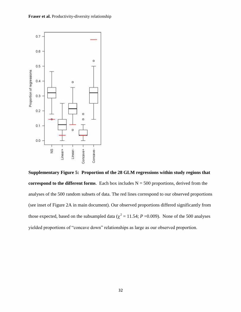
Supplementary Figure 5: Proportion of the 28 GLM regressions within study regions that

correspond to the different forms. Each box includes N = 500 proportions, derived from the

analyses of the 500 random subsets of data. The red lines correspond to our observed proportions

(see inset of Figure 2A in main document). Our observed proportions differed significantly from

those expected, based on the subsampled data (2 = 11.54; P =0.009). None of the 500 analyses

yielded proportions of “concave down” relationships as large as our observed proportion.


33

Supplementary Figure 6: Histogram of the average biomass range observed within each of

the 500 iterations of site-level analyses. For comparison, the red line shows the average

biomass range (428.7 gm-2

) encompassed by the 48 site-level analyses of Adler et al. (1).

Supplementary Tables


34

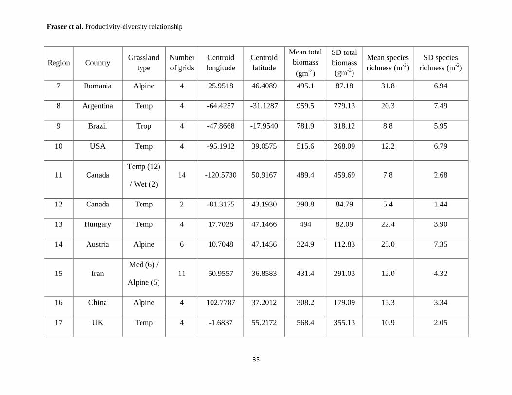
Supplementary Table 1: Herbaceous Diversity Network sites. Grassland type is separated into 5 categories (Temp = temperate;

Wet = temperate wet meadow; Med = Mediterranean; Trop = tropical and subtropical; and Alpine), with numbers in parentheses

indicating number of grids within each grassland type. A grid represents one 8 x 8 m2 sampling area. Coordinates are provided in

decimal degrees, and use the WGS84 datum.

Region Country Grassland

type

Number

of grids

Centroid

longitude

Centroid

latitude

Mean total

biomass

(gm-2

)

SD total

biomass

(gm-2

)

Mean species

richness (m-2

)

SD species

richness (m-2

)

1 Hungary Temp 4 20.1885 46.6159 358.8 267.15 11.7 6.39

2 Germany Temp 6 11.5636 49.9169 412.7 305.22 13.9 8.92

3 Mongolia

Temp (2) /

Wet (4)

6 105.0168 48.8515 317.8 111.90 14.7 4.51

4 Canada Temp 6 -111.9590 50.8912 473.7 317.65 7.6 1.94

5 Canada Temp 6 -111.5615 53.0848 293.9 159.08 13.2 4.33

6 USA Med 2 -117.1685 32.8839 314.2 121.90 7.7 1.62


35


type

Number

of grids

Centroid

longitude

Centroid

latitude

Mean total

biomass

(gm-2

)

SD total

biomass

(gm-2

)

Mean species

richness (m-2

)

SD species

richness (m-2

)

7 Romania Alpine 4 25.9518 46.4089 495.1 87.18 31.8 6.94

8 Argentina Temp 4 -64.4257 -31.1287 959.5 779.13 20.3 7.49

9 Brazil Trop 4 -47.8668 -17.9540 781.9 318.12 8.8 5.95

10 USA Temp 4 -95.1912 39.0575 515.6 268.09 12.2 6.79

11 Canada

Temp (12)

/ Wet (2)

14 -120.5730 50.9167 489.4 459.69 7.8 2.68

12 Canada Temp 2 -81.3175 43.1930 390.8 84.79 5.4 1.44

13 Hungary Temp 4 17.7028 47.1466 494 82.09 22.4 3.90

14 Austria Alpine 6 10.7048 47.1456 324.9 112.83 25.0 7.35

15 Iran

Med (6) /

Alpine (5)

11 50.9557 36.8583 431.4 291.03 12.0 4.32

16 China Alpine 4 102.7787 37.2012 308.2 179.09 15.3 3.34

17 UK Temp 4 -1.6837 55.2172 568.4 355.13 10.9 2.05


36


type

Number

of grids

Centroid

longitude

Centroid

latitude

Mean total

biomass

(gm-2

)

SD total

biomass

(gm-2

)

Mean species

richness (m-2

)

SD species

richness (m-2

)

18 USA

Temp (4) /

Wet (2)

6 -81.6034 41.3593 1592.7 1173.77 2.8 2.58

19 Iran Temp 6 59.0169 36.8936 300.7 184.50 7.0 1.94

20 Brazil Trop 2 -51.6823 -30.1011 215.8 53.01 27.6 5.87

21 Canada Alpine 4 -119.4263 50.0118 280.7 161.03 14.0 3.30

22 Kenya Trop 6 36.8911 0.3882 812.8 451.06 6.0 3.61

23* Israel Med 6 35.5334 32.5213 288.2 169.03 16.7 8.32

24 Japan

Temp (4) /

Wet (2)

6 140.9299 41.0162 545.5 282.98 8.7 4.02

25* Canada Temp 2 -110.4423 49.0361 105.3 37.15 8.1 2.47

26* Mongolia Temp 4 106.9060 49.0153 282.3 94.80 16.1 3.74

27 South Africa Temp 6 29.4935 -25.6213 533.4 327.50 8.0 3.24

28 Italy Alpine 6 13.0179 42.9542 365.3 120.93 19.9 4.92


37


type

Number

of grids

Centroid

longitude

Centroid

latitude

Mean total

biomass

(gm-2

)

SD total

biomass

(gm-2

)

Mean species

richness (m-2

)

SD species

richness (m-2

)

29 New Zealand Temp 2 170.6227 -45.6794 1277 189.75 8.7 1.92

30 Estonia Temp 10 24.7988 58.4634 479 344.14 19.1 8.32

* plant litter was not collected at these sites, so these were excluded from total biomass analyses, but included in live biomass

analyses.


38

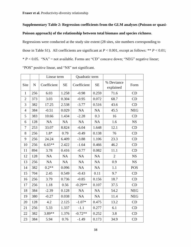
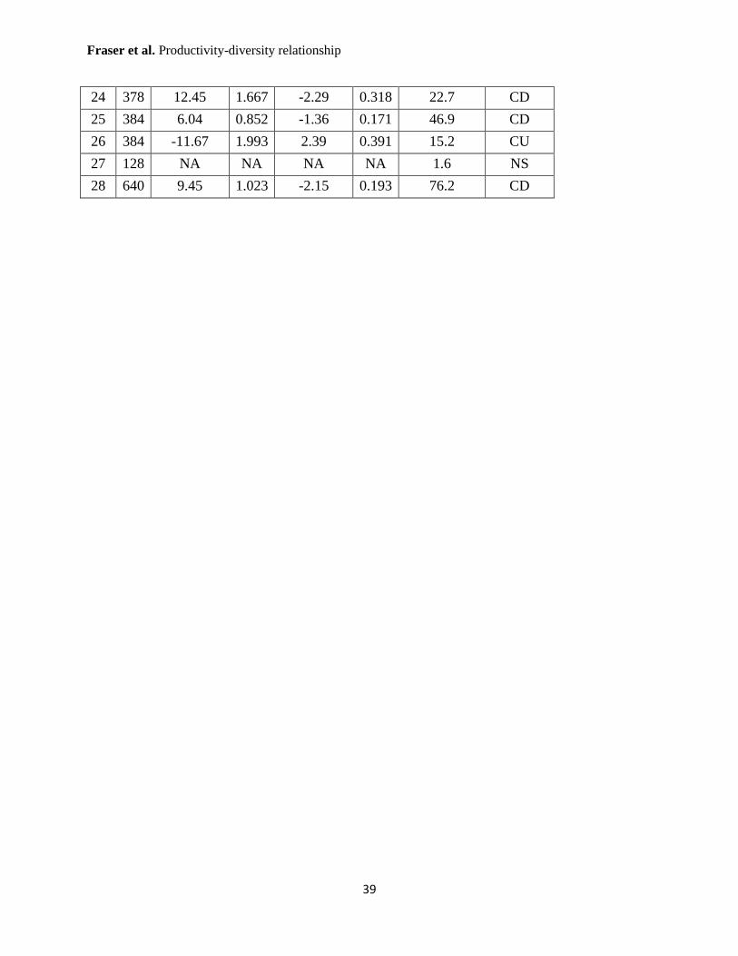
Supplementary Table 2: Regression coefficients from the GLM analyses (Poisson or quasi-

Poisson approach) of the relationship between total biomass and species richness.

Regressions were conducted at the study site extent (28 sites, site numbers corresponding to

those in Table S1). All coefficients are significant at P < 0.001, except as follows: ** P < 0.01;

* P < 0.05. “NA” = not available. Forms are “CD” concave down; “NEG” negative linear;

“POS” positive linear, and “NS” not significant.

Linear term Quadratic term

Site N Coefficient SE Coefficient SE % Deviance

explained Form

1 256 6.03 1.258 -0.98 0.259 71.6 CD

2 373 3.03 0.304 -0.95 0.072 68.7 CD

3 382 17.25 2.538 -3.77 0.516 43.6 CD

4 384 -0.51 0.029 NA NA 45.5 NEG

5 383 10.66 1.434 -2.28 0.3 16 CD

6 128 NA NA NA NA 1.6 NS

7 253 33.07 8.824 -6.04 1.648 12.1 CD

8 256 1.8* 0.79 -0.49 0.138 76 CD

9 256 24.24 6.409 -3.88 1.106 23.3 CD

10 256 6.65** 2.422 -1.64 0.466 46.2 CD

11 894 3.78 0.416 -0.77 0.082 11.1 CD

12 128 NA NA NA NA 2 NS


14 382 0.2** 0.096 NA NA 1.1 POS

15 704 2.45 0.549 -0.43 0.11 9.7 CD

16 256 3.79 0.736 -0.85 0.156 18.7 CD

17 256 1.18 0.56 -0.29** 0.107 37.5 CD

18 384 -2.39 0.128 NA NA 54.2 NEG

19 380 -0.27 0.038 NA NA 11.4 NEG

20 128 4.2 2.125 -1.07* 0.475 13.2 CD

21 256 5.33 1.337 -1.1 0.277 6.1 CD

22 382 3.89** 1.376 -0.72** 0.252 3.8 CD

23 384 5.94 0.76 -1.49 0.173 34.9 CD


39

24 378 12.45 1.667 -2.29 0.318 22.7 CD

25 384 6.04 0.852 -1.36 0.171 46.9 CD

26 384 -11.67 1.993 2.39 0.391 15.2 CU


28 640 9.45 1.023 -2.15 0.193 76.2 CD


40

References (1, 18, 20, 31-36)

1. P. B. Adler et al. Productivity is a poor predictor of plant species richness. Science 333, 1750-

1753 (2011).

18. L. H. Fraser, A. Jentsch, M. Sternberg. What drives plant species diversity? Tackling the

unimodal relationship between herbaceous species richness and productivity. J. Veg. Sci. 25,

1160-1166 (2014).

20. L. H. Fraser et al. Coordinated distributed experiments: an emerging tool for testing global

hypotheses in ecology and environmental science. Front. Ecol. Envir. 11, 147-155 (2013).

31. R Core Team. R: A language and environment for statistical computing. R Foundation for

Statistical Computing, Vienna, Austria. URL http://www.R-project.org/. Version 3.03.

(2014).

32. C. Kleiber, A. Zeileis. Applied Econometrics with R. New York: Springer-Verlag. ISBN

978-0-387-77316-2. URL http://CRAN.R-project.org/package=AER (2008).

33. A. F. Zuur et al. Mixed effects models and extensions in ecology with R. Springer New

York, New York, NY (2009).

34. M. Plummer, in Proceedings of the 3rd International Workshop on Distributed Statistical

Computing, K. Hornik, F. Leisch, A. Zeileis, Eds. (Achim Zeileis, Vienna, Austria,

2003).

35. Y. –S. Su, M. Yajima. R2jags: A Package for Running JAGS from R. R package version

0.04-03. http://CRAN.R-project.org/package=R2jags (2014).

http://cran.r-project.org/package=AER


41

36. A. Gelman, D. B. Rubin. Inference from iterative simulation using multiple sequences.

Statistical Science 7, 457–472 (1992).

worldwide evidence of a unimodal relationship between

Documents