wrsm pitman user manual aug2016
TRANSCRIPT


WATER RESOURCES OF SOUTH AFRICA, 2012 STUDY (WR2012)
WRSM/Pitman User Manual
Report to the Water Research Commission
by
AK Bailey and WV Pitman Royal HaskoningDHV (Pty) Ltd
WRC Report No. TT 689/16
August 2016

Water Resources of South Africa 2012 Study (WR2012): WRSM/Pitman User Manual ii
Obtainable from Water Research Commission Private Bag X03 GEZINA, 0031 [email protected] or download from www.wrc.org.za The publication of this report emanates from a project entitled Water Resources of South Africa, 2012 (WR2012) (WRC Project No. K5/2143/1) and other projects for the Water Research Commission, the Department of Water and Sanitation and for the University of the Witwatersrand. This report forms part of a series of nine reports. The reports are:
1. WR2012 Executive Summary (WRC Report No. TT 683/16) 2. WR2012 User Guide (WRC Report No. TT 684/16) 3. WR2012 Book of Maps (WRC Report No. TT 685/16) 4. WR2012 Calibration Accuracy (WRC Report No TT 686/16) 5. WR2012 SAMI Groundwater module: Verification Studies, Default Parameters and Calibration Guide
(WRC Report No. TT 687/16) 6. WR2012 SALMOD: Salinity Modelling of the Upper Vaal, Middle Vaal and Lower Vaal sub-Water
Management Areas (new Vaal Water Management Area) (WRC Report No. TT 688/16) 7. WRSM/Pitman User Manual (WRC Report No. TT 689/16 – this report) 8. WRSM/Pitman Theory Manual (WRC Report No. TT 690/16) 9. WRSM/Pitman Programmer’s Code Manual WRC Report No. TT 691/16) ISBN 978-1-4312-0851-7 Printed in the Republic of South Africa © WATER RESEARCH COMMISSION

Water Resources of South Africa 2012 Study (WR2012): WRSM/Pitman User Manual iii
Royal HaskoningDHV DISCLAIMER ON WRSM/PITMAN
Although every possible care has been taken in writing the software program WRSM/Pitman*, its operation is open to intentional and unintentional misuse and the results that it produces are open to misinterpretation. For this reason there cannot be any guarantee whatsoever about the correctness of the results produced by the program. TiSD, the authors and supporters (WRC and DWS) of WRSM/Pitman will therefore not take any responsibility whatsoever for damages, whatever their nature, resulting either directly or indirectly from the use of the program.
*©Royal HaskoningDHV (Pty) Ltd- 2015
All rights reserved. No part of this material/ publication may be reproduced, stored in a retrieval system, or transmitted, in any form, or by any means, electronic, mechanical, photocopying, recording or otherwise, without prior permission, in writing, in writing, from Royal HaskoningDHV
Water Research Commission DISCLAIMER
This report has been reviewed by the Water Research Commission (WRC) and approved for publication. Approval does not signify that the contents necessarily reflect the views and policies of the WRC, nor does mention of trade names or commercial products constitute endorsement or recommendation for use.

Water Resources of South Africa 2012 Study (WR2012): WRSM/Pitman User Manual iv
ACKNOWLEDGEMENTS
The authors would like to acknowledge:
The Water Research Commission for their commissioning and funding of this entire project. The Department of Water and Sanitation for their rainfall, streamflow, Reservoir Record and water quality data, some GIS maps and their participation on the Reference Group. The South African Weather Services (SAWS) for their rainfall data.
The following firms and their staff who provided major input:
Royal HaskoningDHV (Pty) Ltd: Mr Allan Bailey, Dr Marieke de Groen, Miss Kerry Grimmer (now WSP Group), Mr Sipho Dingiso, Miss Saieshni Thantony, Miss Sarah Collinge, Mr Niell du Plooy and consultant Dr Bill Pitman (all aspects of the study);
SRK Consulting (SA) (Pty) Ltd: Ms Ansu Louw, Miss Joyce Mathole and Ms Janet Fowler (Land use and GIS maps);
Umfula Wempilo Consulting cc: Dr Chris Herold (water quality); Alborak: Mr Grant Nyland (model development); GTIS: Mr Töbias Goebel (website) and WSM: Mr Karim Sami (groundwater).
The following persons who provided input into the coding of the WRSM/Pitman model:
Dr Bill Pitman; Mr Allan Bailey; Mr Grant Nyland; Mrs Riana Steyn and Mr Pieter van Rooyen.
Other involvement as follows:
Many other organizations and individuals provided information and assistance and the contributions were of tremendous value.

Water Resources of South Africa 2012 Study (WR2012): WRSM/Pitman User Manual v
REFERENCE GROUP
Reference Group Members
Mr Wandile Nomquphu (Chairman) Water Research Commission
Mrs Isa Thompson Department of Water and Sanitation
Mr Elias Nel Department of Water and Sanitation (now retired)
Mr Fanus Fourie Department of Water and Sanitation
Mr Herman Keuris Department of Water and Sanitation
Dr Nadene Slabbert Department of Water and Sanitation
Miss Nana Mthethwa Department of Water and Sanitation
Mr Kwazi Majola Department of Water and Sanitation
Dr Chris Moseki Department of Water and Sanitation
Professor Denis Hughes Rhodes University
Professor Andre Görgens Aurecon
Mr Anton Sparks Aurecon
Mr Bennie Haasbroek Hydrosol
Mr Anton Sparks Aurecon
Mr Gerald de Jager AECOM
Mr Stephen Mallory Water for Africa
Mr Pieter van Rooyen WRP
Mr Brian Jackson Inkomati CMA
Dr Evison Kapangaziwiri CSIR
Dr Jean-Marc Mwenge Kahinda CSIR
Research Team members
Mr Allan Bailey (Project Leader) Royal HaskoningDHV
Dr Marieke de Groen Royal HaskoningDHV
Dr Bill Pitman Consultant to Royal HaskoningDHV
Dr Chris Herold Umfula Wempilo
Mr Karim Sami WSMLeshika
Ms Ans Louw SRK
Ms Janet Fowler SRK
Mr Niell du Plooy Royal HaskoningDHV

Water Resources of South Africa 2012 Study (WR2012): WRSM/Pitman User Manual vi
Mr Töbias Gobel GTIS
Miss Saieshni Thantony Royal HaskoningDHV
Mr Grant Nyland Alborak
Miss Sarah Collinge Royal HaskoningDHV
Miss Kerry Grimmer WSP
Ms Riana Steyn Consultant
Miss Joyce Mathole SRK
Mr Sipho Dingiso Ex Royal HaskoningDHV

Water Resources of South Africa 2012 Study (WR2012): WRSM/Pitman User Manual vii
Table of Contents
OVERVIEW ................................................................................................................................................ xiv
LIST OF ABBREVIATIONS ........................................................................................................................ xx
1 INTRODUCTION ................................................................................................................................ 1 1.1 Hardware requirements ............................................................................................................ 1 1.2 Installation ................................................................................................................................. 2
2 MODULES, ROUTES, INPUT AND OUTPUT FILES ........................................................................ 3 2.1 Modules or sub-models ............................................................................................................ 3 2.2 Routes ...................................................................................................................................... 4 2.3 Input files .................................................................................................................................. 5 2.4 File names in input parameter files........................................................................................... 9 2.5 Changing input datafiles ........................................................................................................... 9 2.6 NETWORK VISIO ..................................................................................................................... 9
3 DATA REQUIREMENTS .................................................................................................................. 11
4 OUTPUT FILES ................................................................................................................................ 12 4.1 Parameter files........................................................................................................................ 12 4.2 Statistics files .......................................................................................................................... 12 4.3 Summary files ......................................................................................................................... 13 4.4 Debug files (obsolete) ............................................................................................................. 13 4.5 Answer files ............................................................................................................................ 13 4.6 Demand files ........................................................................................................................... 15 4.7 Supply files (obsolete) ............................................................................................................ 15 4.8 Shortage files .......................................................................................................................... 16 4.9 Error File ................................................................................................................................. 17 4.10 Print file ................................................................................................................................... 17
5 GRAPHICS ....................................................................................................................................... 18
6 USING WRSM/Pitman ..................................................................................................................... 19 6.1 First Steps ............................................................................................................................... 19 6.2 More Advanced Operations and Configurations .................................................................. 124 6.3 Assorted other Operations .................................................................................................... 151 6.4 Other Messages and Warnings ............................................................................................ 161 6.5 Knowledge Base Articles ...................................................................................................... 162
7 DOs and DON'Ts ........................................................................................................................... 168 7.1 DO: ....................................................................................................................................... 168 7.2 DON'T: .................................................................................................................................. 168
8 DEFICIT HANDLING ...................................................................................................................... 169
9 DEFAULT PARAMETERS ............................................................................................................. 172 9.1 Categories of default input variables/parameters ................................................................. 172
10 CALIBRATION ............................................................................................................................... 177 10.1 Surface water component calibration ................................................................................... 177 10.2 Groundwater component calibration .................................................................................... 182
11 THE DAILY TIME STEP VERSION ................................................................................................ 186 11.1 Edit menu – Network module ............................................................................................... 188 11.2 Edit menu – Runoff module .................................................................................................. 188 11.3 Daily naturalised flow option – Plot menu ............................................................................ 196 11.4 File menu .............................................................................................................................. 197 11.5 Converting from systems set up from previous monthly time step ....................................... 197 11.6 Daily simulated flow option including land use ..................................................................... 198

Water Resources of South Africa 2012 Study (WR2012): WRSM/Pitman User Manual viii
REFERENCES .......................................................................................................................................... 202
APPENDIX A: GRAPH MANUAL ............................................................................................................ 203

Water Resources of South Africa 2012 Study (WR2012): WRSM/Pitman User Manual ix
List of Tables
Table 2.1: Maximum number of routes ................................................................................................. 5 Table 4.1: Maximum number of routes ............................................................................................... 14 Table 9.1: Default Information for Data and Sami and Hughes Parameters .................................... 173 Table 10.1: Parameter effect on simulated flow (Pitman method) ..................................................... 180 Table 10.2: Perennial rivers (sub-surface flow important) .................................................................. 181 Table 10.3: Intermittent rivers (sub-surface flow insignificant) ........................................................... 181 Table 10.4: Effects on simulated flows of model parameter adjustments (Sami method) ................ 182 Table 10.5: Groundwater variable analysis for “total recharge” ........................................................ 183 Table 11.1: Conversion from monthly to daily calibration parameters ............................................... 199
List of Figures
Figure 6.1: A Map of a Portion of the Upper Crocodile River .............................................................. 19 Figure 6.2: The system diagram of Sub-catchment 1 of the Upper Crocodile River ........................... 20 Figure 6.3: The Main Menu Toolbar .................................................................................................... 21 Figure 6.4: The New Network dialog ................................................................................................... 22 Figure 6.5: The Dialog to Choose a Folder ......................................................................................... 23 Figure 6.6: The Create Directory (Create Folder) dialog ..................................................................... 23 Figure 6.7: The toolbar when a Network is open ................................................................................. 24 Figure 6.8: The status bar at the bottom of the main program window ............................................... 25 Figure 6.9: Creating a new Runoff Module .......................................................................................... 25 Figure 6.10: The Edit | Runoff Modules > General Dialog ..................................................................... 26 Figure 6.11: The Missing MAP dialog .................................................................................................... 28 Figure 6.12: The Edit | Runoff Modules > Climate ................................................................................ 28 Figure 6.13: The Missing Rainfile Dialog ............................................................................................... 28 Figure 6.14: The Create New Runoff Module dialog (2) ........................................................................ 29 Figure 6.15: The File | Create Rainfile Dialog ....................................................................................... 29 Figure 6.16: The Catchment Rainfall Massplot ..................................................................................... 31 Figure 6.17: The Catchment Rainfall CUSUM plot ................................................................................ 32 Figure 6.18: The Edit | Runoff Modules dialog ...................................................................................... 34 Figure 6.19: The Edit | Runoff Modules > Climate dialog ...................................................................... 35 Figure 6.20: The Edit | Runoff Modules > Calibration dialog ................................................................. 37 Figure 6.21: The Select Runoff Modules for Applying Calibration Parameters Dialog .......................... 39 Figure 6.22: The Edit | Runoff Module > Groundwater dialog ............................................................... 40 Figure 6.23: Edit | Runoff Modules > Sami GW ..................................................................................... 44 Figure 6.24: The File | Add New | Channel Module dialog .................................................................... 47 Figure 6.25: The Edit | Channel Module > General dialog .................................................................... 47 Figure 6.26: The File | Add New | Route dialog ..................................................................................... 48 Figure 6.27: The File | Add New | Route dialog, filled out ..................................................................... 49 Figure 6.28: The Edit | Runoff Module | Outflow dialog ......................................................................... 49 Figure 6.29: The File | Add New | Route dialog for the Channel Module outflow route ........................ 50

Water Resources of South Africa 2012 Study (WR2012): WRSM/Pitman User Manual x
Figure 6.30: The Edit | Route > Defined Flows dialog ........................................................................... 50 Figure 6.31: The Illegal Primary Outflow route dialog ........................................................................... 51 Figure 6.32: The Edit | Channel Module | Outflows dialog .................................................................... 52 Figure 6.33: The Simulation Successful dialog ..................................................................................... 52 Figure 6.34: The File | Add New | Gauging Station dialog .................................................................... 53 Figure 6.35: The Edit | Gauging Station | General dialog ...................................................................... 53 Figure 6.36: The Output File Check dialog ............................................................................................ 55 Figure 6.37: The Edit | Network > Global dialog .................................................................................... 55 Figure 6.38: The View | Runoff Modules dialog ..................................................................................... 57 Figure 6.39: The Edit | Network > Module Sequence dialog ................................................................. 58 Figure 6.40: The Edit | Network > Summary Dialog .............................................................................. 59 Figure 6.41: The Program Toolbar after a successful Simulation ......................................................... 59 Figure 6.42: The View | Statistics dialog................................................................................................ 60 Figure 6.43: The Plot | Plot Dialog ......................................................................................................... 63 Figure 6.44: The Monthly Hydrograph Plot ............................................................................................ 64 Figure 6.45: The Annual Hydrograph Plot ............................................................................................. 64 Figure 6.46: The Mean Monthly Flows Plot ........................................................................................... 65 Figure 6.47: The Gross Yield Plot.......................................................................................................... 66 Figure 6.48: The Scatter Diagram ......................................................................................................... 67 Figure 6.49: The Monthly Histogram ..................................................................................................... 67 Figure 6.50: The Cumulative Frequency Plot ........................................................................................ 68 Figure 6.51: The Reservoir Trajectory Plot ............................................................................................ 69 Figure 6.52: The Groundwater Surface water Plot ................................................................................ 70 Figure 6.53: The Daily Hydrograph – naturalised flow .......................................................................... 71 Figure 6.54: The Daily Hydrograph including land use ......................................................................... 72 Figure 6.55: The Streamflow Massplot .................................................................................................. 73 Figure 6.56: The Streamflow CUSUM Plot ............................................................................................ 74 Figure 6.57: The Firm Yield – Storage Plot ........................................................................................... 75 Figure 6.58: Plot | Hardcopy Options | Drivers Dialog ........................................................................... 76 Figure 6.59: The Edit | Irrigation Module > General dialog .................................................................... 77 Figure 6.60: The Edit | Irrigation Module > Climate dialog .................................................................... 79 Figure 6.61: The Check MAP Dialog ..................................................................................................... 79 Figure 6.62: The View | Routes dialog................................................................................................... 81 Figure 6.63: The Missing Area Data Dialog in Irrigation Blocks ............................................................ 81 Figure 6.64: The Edit | Irrigation Modules > Area dialog ....................................................................... 82 Figure 6.65: The Output file check dialog .............................................................................................. 83 Figure 6.66: The Sequence error dialog ................................................................................................ 83 Figure 6.67: The simulation failed dialog ............................................................................................... 83 Figure 6.68: The View | Routes dialog................................................................................................... 84 Figure 6.69: The Edit | Network > Module sequence dialog .................................................................. 84 Figure 6.70: The Edit | Reservoir Modules > General dialog ................................................................ 86 Figure 6.71: The missing inflow routes dialog for Reservoirs ................................................................ 86 Figure 6.72: The Edit | Runoff Modules > Outflow dialog ...................................................................... 87 Figure 6.73: The Edit | Route | Defined Flows dialog ............................................................................ 88 Figure 6.74: The Illegal spillage route dialog for Reservoirs ................................................................. 88

Water Resources of South Africa 2012 Study (WR2012): WRSM/Pitman User Manual xi
Figure 6.75: The Edit | Reservoir Modules > Outflow dialog ................................................................. 89 Figure 6.76: The missing MAP dialog for Reservoirs ............................................................................ 90 Figure 6.77: The Edit | Reservoir Modules > Climate dialog ................................................................. 90 Figure 6.78: The Missing Year/Area/Volume Data Dialog for Reservoirs ............................................. 91 Figure 6.79: The Edit Reservoir > Storage dialog ................................................................................. 91 Figure 6.80: The sequence error dialog ................................................................................................ 92 Figure 6.81: The Edit | Network Module > Sequence dialog ................................................................. 93 Figure 6.82: A monthly hydrograph plot ................................................................................................ 93 Figure 6.83: The Edit | Irrigation Modules > Crops dialog ..................................................................... 94 Figure 6.84: The Edit | Irrigation Modules > Allocation dialog for the Pitman Irrigation Model ............. 95 Figure 6.85: The Edit | Irrigation Modules > Crops2 dialog ................................................................... 96 Figure 6.86: The Edit | Irrigation Modules > Allocation dialog for the WQT, WQT-SAPWAT and WQT
Type 4 Irrigation Models .................................................................................................... 97 Figure 6.87: The Edit | Irrigation Module > Canal dialog ....................................................................... 99 Figure 6.88: The Edit | Irrigation Modules > Groundwater Dialog ....................................................... 100 Figure 6.89: The Edit | Irrigation Modules > Efficiency dialog ............................................................. 102 Figure 6.90: The File | Add New | Route dialog ................................................................................... 103 Figure 6.91: The View | Routes dialog................................................................................................. 104 Figure 6.92: The Edit | Routes > Defined Flows dialog ....................................................................... 104 Figure 6.93: The Edit | Irrigation Modules > Return Flows dialog for the Pitman Irrigation model ...... 105 Figure 6.94: The Edit | Irrigation Modules > Return Flows dialog for the WQT, WQT-SAPWAT or
WQT Type 4 Irrigation models ........................................................................................ 106 Figure 6.95: The Edit | Irrigation Modules > Capacity dialog for the WQT Type 4 Irrigation models. . 107 Figure 6.96: Generic coal mining water modelling system .................................................................. 109 Figure 6.97: Typical opencast pit layout .............................................................................................. 110 Figure 6.98: Schematic showing model representation in opencast pit .............................................. 110 Figure 6.99: Rehabilitated pit with the water level at the weathered zone. ......................................... 111 Figure 6.100: Schematic representation of underground mine used in model ...................................... 112 Figure 6.101: Schematic representation of discard dump in model ...................................................... 113 Figure 6.102: The Edit | Mining Module > General dialog for the WRSM/Pitman Mining Module ........ 114 Figure 6.103: The Edit | Mining Module > Climate dialog for the WRSM/Pitman Mining Module ......... 115 Figure 6.104: The Edit | Mining Module > Outflow dialog for the WRSM/Pitman Mining Module ......... 116 Figure 6.105: The Edit | Mining Module > Plant dialog for the WRSM/Pitman ...................................... 116 Figure 6.106: The Edit | Mining Module | Section > Opencast Section dialog for the WRSM/Pitman
Mining Module ................................................................................................................. 117 Figure 6.107: The Edit | Mining Module | Section > Underground Section dialog for the WRSM/Pitman
Mining Module ................................................................................................................. 117 Figure 6.108: The Edit | Mining Module | Section > Dump Area Section dialog for the WRSM/Pitman
Mining Module ................................................................................................................. 118 Figure 6.109: The File | Save | Route Flows dialog ............................................................................... 118 Figure 6.110: The File | Save | Reservoir Storages dialog .................................................................... 119 Figure 6.111: File | Save | Module time series | Runoff Modules .......................................................... 120 Figure 6.112: File | Save | Module time series | Channel Modules ....................................................... 121 Figure 6.113: File | Save | Module time series | Mining Modules .......................................................... 122 Figure 6.114: File | Convert | “.ANS” to “.CSV” and File | Convert | “.CSV” to “.ANS” .......................... 123 Figure 6.115: The network not saved dialog ......................................................................................... 124

Water Resources of South Africa 2012 Study (WR2012): WRSM/Pitman User Manual xii
Figure 6.116: The “do you want to save” Dialog .................................................................................... 124 Figure 6.117: The Load Network File Dialog ......................................................................................... 125 Figure 6.118: The Edit | Runoff Module > Afforestation dialog .............................................................. 126 Figure 6.119: The missing area data dialog .......................................................................................... 126 Figure 6.120: The Edit | Runoff Module | Alien Vegetation dialog ......................................................... 128 Figure 6.121: Edit | Runoff Modules > General Dialog .......................................................................... 131 Figure 6.122: Edit | Runoff Modules > General (SL1 – Forest) Dialog .................................................. 132 Figure 6.123: Edit | Runoff Modules > General (SL2 – Cane) Dialog ................................................... 133 Figure 6.124: Edit | Runoff Modules > General (Parent Catchment) Dialog ......................................... 134 Figure 6.125: Create | Runoff Modules > SFR Children Dialog ............................................................ 134 Figure 6.126: Edit | Runoff Modules > General (SL2 – Forest) dialog .................................................. 135 Figure 6.127: Edit | Runoff Modules > Afforestation (SL1 – Forest) Dialog .......................................... 136 Figure 6.128: Edit | Runoff Module > Afforestation – Smoothed Gush/Pitman ..................................... 137 Figure 6.129: Edit | Runoff Modules > Afforestation – User Defined..................................................... 137 Figure 6.130: The Edit | Runoff Modules > Paved dialog ...................................................................... 142 Figure 6.131: The Edit | Channel Modules > General dialog ................................................................ 143 Figure 6.132: The Edit | Channel Modules > Climate dialog ................................................................. 144 Figure 6.133: The Edit | Channel Modules > Wetlands(B) dialog ......................................................... 145 Figure 6.134: The Edit | Channel Modules > Wetlands(C) dialog ......................................................... 146 Figure 6.135: The Edit | Channel Modules > Diversion dialog .............................................................. 147 Figure 6.136: The New Route dialog ..................................................................................................... 150 Figure 6.137: The Route parameter dialog ............................................................................................ 150 Figure 6.138: The Reservoir restrictions dialog ..................................................................................... 151 Figure 6.139: The Import Dialog ............................................................................................................ 152 Figure 6.140: The Module Number Conflict Dialog ............................................................................... 152 Figure 6.141: The import module, input file error .................................................................................. 153 Figure 6.142: The Delete Module Dialog ............................................................................................... 153 Figure 6.143: The zero route check dialog ............................................................................................ 154 Figure 6.144: Viewing the Routes.......................................................................................................... 155 Figure 6.145: Deleting a Route .............................................................................................................. 155 Figure 6.146: Adding a New Route 7 .................................................................................................... 156 Figure 6.147: Adding a defined flow ...................................................................................................... 156 Figure 6.148: The New Channel Module dialog .................................................................................... 157 Figure 6.149: Add a New Route 2 ......................................................................................................... 157 Figure 6.150: The Hardcopy Options .................................................................................................... 158 Figure 6.151: The Print Module(s) Dialog .............................................................................................. 159 Figure 6.152: Help | About | About WRSM 2000 Dialog ........................................................................ 160 Figure 6.153: The DLL Load Error Dialog ............................................................................................. 161 Figure 6.154: The Old-DLL Dialog ......................................................................................................... 162 Figure 10.1: Statistics using the Pitman methodology ........................................................................ 178 Figure 11.1: Flowchart of daily time step process ............................................................................... 187 Figure 11.2: The Daily Time Step Network .......................................................................................... 188 Figure 11.3: The Runoff Module with Daily Time Step Calibration Property Tab ................................ 189 Figure 11.4: The Runoff Module with Daily Time Step Calibration Screen ......................................... 189 Figure 11.5: Create a Daily Land Use File and Daily Flow Conversions screen ................................. 192

Water Resources of South Africa 2012 Study (WR2012): WRSM/Pitman User Manual xiii
Figure 11.6: The Runoff Module with Climate Screen ......................................................................... 196 Figure 11.7: The Plot menu with Daily Hydrograph – naturalised ....................................................... 196 Figure 11.8: The Daily Hydrograph – naturalised ................................................................................ 197 Figure 11.9: The Daily Flows Time Series Output ............................................................................... 197 Figure 11.10: Determining a daily simulated flow file (including land use) ............................................ 200 Figure 11.11: The Plot menu with Daily Simulated Hydrograph – including land use ........................... 200 Figure 11.12: The Daily Simulated versus Observed Hydrograph – including land use ....................... 201

Water Resources of South Africa 2012 Study (WR2012): WRSM/Pitman User Manual xiv
OVERVIEW
WRSM/Pitman is a mathematical model to simulate the movement of water through an interlinked system of catchments, river reaches, reservoirs, irrigation areas and mines. WRSM2000 is of a modular construction (running under Windows), with five different types of module (runoff, reservoir, irrigation, channel and mining) linked by means of routes. The routes represent lines along which water flows, such as river reaches.
The model was first developed in 1969 and has been subject to numerous enhancements over the years. There have been various name changes but it is currently known as either the WRSM2000 model or the Pitman model. This manual will refer to it as WRSM/Pitman.
There are currently three versions of the model as follows:
• WRSM/Pitman version 2.7 which is a monthly time step version which has been used for the WR2005 and WR2012 study for the Water Research Commission and has been the version available over the past 10 years or so.
• WRSM/Pitman version 2.6 which is a daily time step version and has been distributed to certain people in 2013 and 2014. It also has the monthly time step but users are recommended to use it only for daily time step analyses and
• WRSM/Pitman version 2.9 which is the latest version and has a number of enhanced features as developed during the WR2012 study such as the irrigation Type 4 methodology, new graphs for rainfall and naturalised flow, observed levels for dams graphs, multiple runoff module calibration, time series of groundwater abstractions and enhanced zooming, panning, etc. of graphs.
WRSM/Pitman has been used to analyse the hydrology on a monthly time scale for a number of diverse applications ranging from very small to very large catchments varying in complexity from being totally undeveloped to highly developed. It has been used throughout South Africa, SADC countries and even in certain overseas countries. It has also been used to analyse catchments on a daily time step such as the Nylsvlei catchment.
Some common uses of the model are:
• to calibrate streamflow records taking land-use changes over time into account by comparing the observed flows against those simulated by the model;
• for broad regional assessment of water resources; • to produce naturalised flow records, i.e. take out man-made land-use effects; • to estimate flows in ungauged catchments by transferring parameters; • when the density of flow gauges is insufficient to cover all catchments, when record periods are too short
and/or when records show changes in land-use over time; • simple reservoir yield analysis; • input to complex system models of water resources (e.g. WRYM, WRPM); • input to water quality studies and • input to Ecological Water Requirement models.
The model is not appropriate for flood design and for determining yields of dams in a complex system of competing water users.
Each of the 5 modules contains one (or offers a choice between more than one) hydrological models that simulate a particular hydrological aspect. The modules are linked to one another by means of routes.

Water Resources of South Africa 2012 Study (WR2012): WRSM/Pitman User Manual xv
Multiple instances of the different modules, together with the routes, form a network. By choosing and linking several modules judiciously, virtually any real-world hydrological system can be represented.
The first step in simulating any hydrological system is to set up the network of modules and routes to represent this system. The Windows version of WRSM/Pitman allows for much larger networks than ever before and offers interactive creation and editing of all modules, routes and networks. The program supports the user by means of extensive error checking and does away with the error-prone and time consuming chore of creating data files in an editor, external to the program. Where files of older versions of the program are supplied, WRSM/Pitman will automatically update these files to be compatible to this latest version.
WRSM/Pitman simulates flows in a catchment and by comparing against observed flows, the user can analyse statistics and graphs of various water resource parameters and manipulate calibration parameters to achieve a good ‘fit’ between observed and simulated flows. Once this has been achieved for the network, naturalised flows can be determined, i.e. flows without any man-made effects of reservoirs, industry, towns, irrigation schemes, mines, etc.
ROUTES
Each module is connected to other modules by means of routes. Routes can be visualised as loss free river reaches, canals or pipelines connecting the various modules to one another to form a coherent network.
A route is always bounded by two modules: a source module and a sink module. Flow along a route will be from the source to the sink module. All modules can, under certain circumstances, be both source and sink modules. Reservoir and channel modules can be both source and sink modules but an irrigation module is usually a sink module. If an irrigation module has a return flow route, it is also a source module.
A collection of modules and routes is called a network. Routes can convey water from a source – or to a sink – outside the network. Such routes are bounded by zero modules external to the network. There are two types of zero modules – zero source modules and zero sink modules. Zero source modules bring flows into the network and zero sink modules lead flows out of the network. Flows along routes that originate in zero source modules must be defined by means of a file of monthly values. Routes that terminate in a zero sink module may be defined by means of a file of monthly flows or may be left undefined if this route is the principal outflow route of the network. Outflow routes from reservoir modules have the added feature that they may be defined as monthly defined abstraction flows, but such routes do not necessarily have to terminate in a zero sink module; they may also flow into a downstream channel module or a different reservoir module.
MODULES OR SUB-MODELS
The terms modules or sub-models have the same meaning. Those familiar with routing theory may prefer the term node, but we will use the terms module or sub-model.
WRSM/Pitman is totally modular. This means that a number of modules can be linked together in any feasible way to form a network. This Windows version does not restrict the user to a maximum number of modules as was the case with the DOS version. Memory is allocated dynamically and therefore the size of network is limited only by the memory available.

Water Resources of South Africa 2012 Study (WR2012): WRSM/Pitman User Manual xvi
RUNOFF MODULE
The runoff module is the heart of WRSM/Pitman and it retains a strong similarity to the original Pitman model. The user should note the following:
(a) pan factors are read in as data, i.e. they are not built into the program. Normally Symons pan evaporations are used in the runoff module, but the user could adopt A-pan figures, provided suitable "crop factors" are available for natural vegetation;
(b) the growth of afforestation, impervious areas and alien vegetation is represented by reading in values for up to ten different years. The most recent research on afforestation (Smoothed Gush/Pitman) has been added as the default with the CSIR method of afforestation and Van der Zel afforestation retained as options. A user defined option has also been added whereby the user enters the required MAR and low flow reductions. LUT Gush is a further option that has not yet been implemented. Additional afforestation data for Pine, Eucalypt and Wattle is required. Alien vegetation has been incorporated in this (version 3) of the model and it follows a similar approach as for afforestation with classifications for tall trees, medium trees and tall shrubs;
(c) the module also has the facility to send fixed proportions of the total runoff along various routes. This feature enables one to economise on runoff modules in relatively homogeneous areas and
(d) groundwater-surface water interaction has been implemented with the choice of either the Hughes or Sami groundwater models.
CHANNEL MODULE
The main function of the channel module is to collect the inflows to it from various routes and to re-distribute these flows along the outflow routes.
Inflows can be in the form of predefined flows or calculated outflows from any of the five types of modules. Channel modules can therefore be sink modules for routes from other channel modules.
Outflows can also be predefined flows but are more often calculated demands from adjacent irrigation modules. The principal outflow route represents the main river channel and surplus flow is passed along this route after all demands are satisfied.
The channel module also makes provision for bed losses and evaporative losses from a wetland area.
There are two options for wetlands – a simplified and more complex method.
If there is a wetland to be simulated, both options require as input a set of twelve monthly pan values and associated pan factors. A rainfile and MAP must also be specified so that the net evaporative loss can be computed. The more complex option requires additional data as specified later in this document.
RESERVOIR MODULE
The reservoir module can be used to represent a single reservoir or an equivalent dam made up of any number of small dams. Allowance is made for the single dam to be constructed (and raised) in any year during the simulation period and for the number of small dams to change over time by inputting values of storage and surface area for up to ten different years.

Water Resources of South Africa 2012 Study (WR2012): WRSM/Pitman User Manual xvii
Evaporation is calculated in a similar way to that for wetlands and one has complete flexibility in the choice of pan type and the associated pan factors.
The reservoir module collects inflows and distributes outflows in a manner similar to that described for the channel module. The one essential difference is the effect of storage, which means that the reservoir must be filled before outflow can take place along the principal outflow (i.e. spillage) route.
IRRIGATION MODULE
Four methods are available for irrigation modules, namely the original method, the WQT method, the WQT-SAPWAT method – WRSM2000 Theory (Stewart Scott, 2006) and the WQT Type 4 method. For the original method, the user should note the following:
(a) changes of irrigation area over time can be represented by inputting values for up to ten years;
(b) the choice of pan type and pan factor is left to the user (A-pan data with associated crop factors would normally be preferred);
(c) MAP of the irrigation area and its rainfall pattern need not be the same as the catchment (runoff module) in which it lies geographically; and
(d) a limit (in mm) can be placed on the abstraction in any one year and effective rainfall factors can be read in for each month.
The module also allows for a seasonal cropping pattern in the form of twelve monthly factors giving the area irrigated as a proportion of the total area. Return flow, as a percentage of the application, can take place along a specified route.
The WQT, WQT-SAPWAT and WQT Type 4 methods require additional data as specified later in this document.
WQT-SAPWAT is similar to the WQT method and has been included to make use of more detailed irrigation requirement data from registration and validation information of all crop-irrigation system combinations. In this case an inventory of monthly crop requirements is identified for each combination using SAPWAT (discounting rainfall and effective rainfall). Each monthly crop-irrigation system SAPWAT requirement is area weighted (outside of WRSM/Pitman) to obtain a single representative crop monthly requirement (mm).
The user can also opt to use drought reduction factors (set in the Climate input screen) for either the WQT, WQT-SAPWAT or WQT Type 4 methods. These factors are aimed at supplemental irrigation planting practices, i.e. in dry months planting will be delayed until it rains and in dry years the total irrigation will be reduced. These factors are not applicable in areas where there is a high supply of water compared to the demand such as Orange River irrigators in Upington. These drought reduction factors (between 0 and 1) will be applied to reduce the flows in routes to and from the irrigation block.
For the above two methods, there is an option in the “Allocations” input screen to have either proportional reduction, i.e. if the allocation limit specified is reached, then all the months get reduced proportionally (as is the case with the original method) or to clip only those months where the allocation (reduced evenly to a monthly value) is exceeded. The annual allocation limit is applied to the end of period area specified and adjustments are made prior to that. For both options, there may be some months that have higher flows than without any allocation limit – this is due to a re-distribution of flow based on the fact that some months are now lower. The default is proportional reduction.
Water Resources of South Africa 2012 Study (WR2012): WRSM/Pitman User Manual xviii
MINING MODULE
Mining modules are used to simulate the runoff that is generated by a mining concession. The hydrological component of the mining module is identical to the mining module that was developed as part of the WQS model by Mr Van Rooyen of WRP and Mr Coleman of Golder and Associates.
A small portion of a catchment is defined as a mining module. This mining module is then divided into plant area and 3 possible different section types. A section type can either be an opencast working, an underground working and/or a slurry/dump area. Opencast workings are further subdivided into pre-strip, pit and rehabilitated areas. Underground workings can be either board and pillar areas or high extraction areas.
Each mining module can contain one plant area and up to 10 each of the three types of sections. Outflow of each section may be routed directly to a river or to a central pollution control dam via an outflow route. Certain sections may also have smaller intermediate pollution control dams that spill into the central pollution control dam.
GAUGING STATIONS
Gauging stations are associated with routes and contain data about historically observed flows. Gauging stations are used to compare the simulated flows with observed flows in a route, so that the calibration of the network can be achieved. It is important to distinguish a gauging station on a route from a defined flow in a route. Gauging stations are used for comparison only whereas defined flows push or pull the flows in the model.
NETWORK
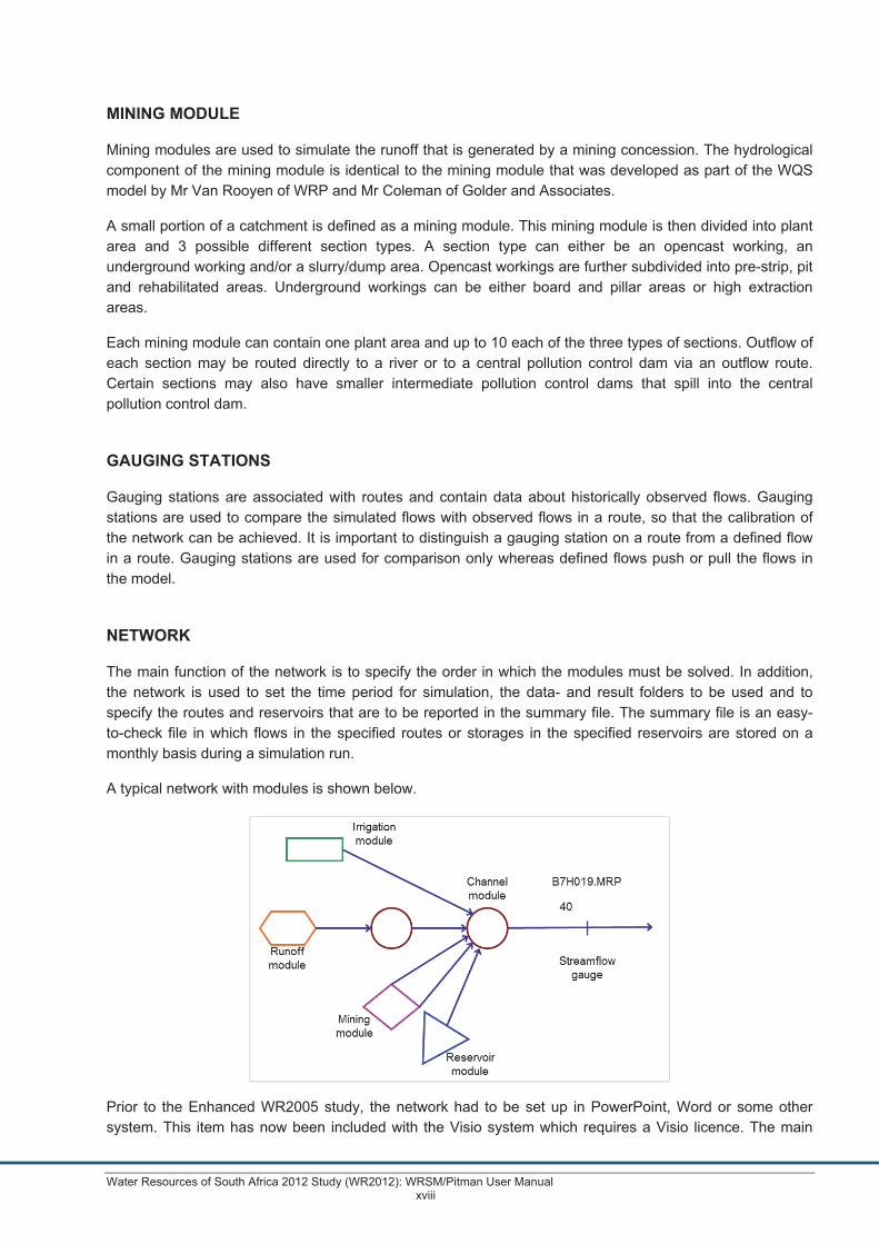
The main function of the network is to specify the order in which the modules must be solved. In addition, the network is used to set the time period for simulation, the data- and result folders to be used and to specify the routes and reservoirs that are to be reported in the summary file. The summary file is an easy-to-check file in which flows in the specified routes or storages in the specified reservoirs are stored on a monthly basis during a simulation run.
A typical network with modules is shown below.
Prior to the Enhanced WR2005 study, the network had to be set up in PowerPoint, Word or some other system. This item has now been included with the Visio system which requires a Visio licence. The main
Water Resources of South Africa 2012 Study (WR2012): WRSM/Pitman User Manual xix
advantage of Visio is to ensure that there is compatibility between the network diagram and what is in the system datafiles, i.e. elimination of errors that occur when there is no link with WRSM/Pitman and the network diagram. Another advantage is the standardisation of the appearance of modules and routes.
A feature has been included in WRSM/Pitman to view the network diagram (must be in pdf form) set up for the relevant catchment.
RAINFILES
A rainfile is a file that contains a monthly rainfall time series expressed as percentages of MAP for an area or a catchment. Rainfiles should not be confused with raingauge files. A rainfile usually combines the data of multiple raingauges into a single time series and, in addition, the values are expressed as a percentage of the MAP for the area or catchment. In the past, rainfiles were generated by means of a separate program called HDYP08. Year 2000 compatible rainfiles can now be created by means of WRSM/Pitman.
It should be noted that raingauge files must be set up by converting the source format to that required by WRSM/Pitman as well as to patch these files (should this be required). If you are in any doubt as to the mechanics of this process, you could consult one of the authors of this document, namely: Mr Allan Bailey of Royal HaskoningDHV.
OPERATION
Operation of WRSM/Pitman is facilitated by a Windows style main menu that gives a number of options to the user, including building a network, running the simulation, viewing statistics, plotting graphs, changing model parameters and writing results to output devices. The model stores all information internally, so that any number of runs can be undertaken without terminating the program. This facility, in conjunction with the ability to look at several gauging points in a network, speeds up the calibration process considerably.

Water Resources of South Africa 2012 Study (WR2012): WRSM/Pitman User Manual xx
LIST OF ABBREVIATIONS
WRSM/Pitman Water Resources Simulation Model
WQT Water Quality Model
SAPWAT Name of a model (source unknown)
SPATSIM Spatial Simulation Framework of Models
WR90 Water Resources of South Africa, 1990 Study
WR2005 Water Resources of South Africa, 2005 Study
Enhanced WR2005 Enhanced Water Resources of South Africa, 2005
WRYM Water Resources Yield Model
WRPM Water Resources Planning Model
WR2012 Water Resources of South Africa, 2012 Study
WRMF Water Resource Modelling Framework

Water Resources of South Africa 2012 Study (WR2012): WRSM/Pitman User Manual 1
1 INTRODUCTION
The program MORSIM was written in 1973 to model runoff from a catchment. This model and the theory behind it are described in HRU Report 2/731. After HRU Report 2/73 was written, program MORSIM was enhanced and became known as HDYP09. This model was used in the 1981 appraisal of South Africa's water resources2.
The computer model WRSM903 (Water Resources Simulation Model 1990) was a refinement and enhancement of the computer model HDYP09. This model used DOS as an operating system. The development of WRSM90 formed part of the “Water Resources 1990“4 project (WR90) undertaken for the Water Research Commission. With the advent of Windows, the fact that WRSM90 was limited to a record period of 80 years and the year 2000 problem, it was decided to produce a Windows version.
WRSM2000 (version 2) had all the same algorithms as WRSM90 and the user could expect identical results if an old DOS network is used. This version solved the year 2000 problem, allowed for a record period of up to 150 years and was a user-friendly Windows program. Memory was assigned dynamically and therefore up to about 1750 modules could be used with 32 MB RAM and about 3500 modules with 64MB RAM. It was easier to create the network file and other modules. The files with rainfall time series as percentage of MAP (rainfiles) were determined as part of the model and the program HDYP08 was no longer required.
For the latest version to be called WRSM/Pitman (version 2.9) as some users refer to it as WRSM2000 while others particularly in other African countries call it the Pitman model, a number of alternative methodologies have been introduced to make the model an integrated water resource model. Of particular significance is the surface-groundwater interaction (both the Hughes and Sami method have been included). Water quality has, however, been excluded and kept separate. All the methodologies available in version 2 have been retained as options. An enhanced graph environment has been provided.
The general theoretical background of the model has, however, remained largely the same. The names of the variables, which have become widely known in the industry, have been retained to ensure continuity.
This report deals with the actual operation of the model and could be seen as a user manual. For details of the theory behind the model, the reader is referred to WRSM2000 Theory (Stewart Scott, 2006)
Users will not receive the source code of this program, but a compiled version or (“.EXE”) file and two DLL files.
1.1 Hardware requirements
The program WRSM/Pitman was written in Lahey Fortran LF90 and its “sister” module Winteracter. Some additional Delphi code has been added. Winteracter is a “Win 32 and Fortran 90 dedicated user interface and graphics development tool which also provides visual tools for menu and “dialog box” design. WRSM/Pitman runs under Windows 7, Windows XP, Windows 95, Windows 98 and NT 4. The program will not run under Windows 3.x.
Any computer that will run one of the recommended operating systems will be adequate to run WRSM/Pitman. A minimum of 32 MB RAM is advised. The size of the networks (i.e. the number of modules and routes within a network) that can be simulated with the program will depend on the
Water Resources of South Africa 2012 Study (WR2012): WRSM/Pitman User Manual 2
amount of available RAM and the size of the swap file in the computer system. The speed of solution of a network will clearly depend on the speed of the processor, but even a 100 MHz Pentium produces acceptable performance. A standard low end graphics adapter with 2 MB RAM with the appropriate driver for the operating system will suffice. A resolution of 800x600 pixels for the monitor is adequate. A lower display resolution is not recommended.
1.2 Installation
The program is supplied as a zipped executable or it can be downloaded from the website www.waterresourceswr2012.co.za. This file should be unzipped to create “WRSM2000.EXE”, “WRENG.DLL” and “WRSM2000DB.DLL”. Both the EXE and the DLLs should be in the same directory. There is a key code required which is machine dependant which has to be obtained from Mr Allan Bailey. One can set up other directory paths for data inside of the model.
If the Visio system is to be used to set up the network diagram, please refer to the OVERVIEW/Network section

Water Resources of South Africa 2012 Study (WR2012): WRSM/Pitman User Manual 3
2 MODULES, ROUTES, INPUT AND OUTPUT FILES
2.1 Modules or sub-models
2.1.1 General
The terms modules and sub-models are interchangeable, and have exactly the same meaning. Those familiar with routing theory will be more comfortable in referring to a sub-model as a node, but we will use the term sub-model or module. The terms are used interchangeably in this manual.
The computer model WRSM/Pitman is totally modular. This means that a number of modules can be strung together in any feasible way to form a network.
The modules (sub-models) that are available are:
(a) The runoff module; (b) The channel reach module; (c) The reservoir module; (d) The irrigation block module; and (e) The mining module.
A network can have a number of the same type of modules. Every sub-model has a sub-model (or module) number.
2.1.2 Maxima
The major difference with regards to maximums between WRSM90 and WRSM/Pitman is that the maximum number of any given modules in a network is 9999. A network could therefore theoretically have 9999 runoff modules, 9999 reservoir modules, 9999 channel modules and 9999 irrigation modules. Modules may be numbered from 1 up to and including 9999. In WRSM/PITMAN it is perfectly valid to have different module types (runoff, channel, irrigation and reservoir) with the same module number (e.g. 122). In that case there would be a module called 122RU, 122CR, 122RR and 122RV in the same network.
The number of modules that can actually be loaded into a particular computer will depend on the size of the RAM on that machine, the size of the swap file that is used and how many programs are open at the time when the program is run.
Memory is allocated and de-allocated dynamically as and when the program needs it. Once a low memory error occurs, the program will issue a warning. Deleting a few modules or routes could solve the problem, but since contiguous blocks of memory need to be allocated, it is not guaranteed that one could, for example, delete a few runoff modules (which use relatively little memory) and hope that it is then possible to add another route (which would need a much larger block of contiguous memory). In order to make the program 'push' all the memory that it uses 'together' it could help to minimise the main program Window by clicking on the '-' (minimise) button and then to maximise the program Window again.

Water Resources of South Africa 2012 Study (WR2012): WRSM/Pitman User Manual 4
2.1.3 Internal files
Since the program now has perfectly adequate editing facilities to add and import modules into a network or to delete modules from a network and to edit the actual module data, it should no longer be necessary to edit the data files directly.
The network and module files are still stored in plain ASCII text in the input folder. It is not recommended that the user edits them directly – neither with the Edit | Any file menu point, nor with any editor since mistakes are increased dramatically with manual editing. The Edit | Any file option is provided solely to edit defined flows or defined abstraction files or to add comments to result files if necessary.
When saving a network, all the data files for all the modules that were changed by means of the WRSM/Pitman editing facility are automatically saved in the place of the originals in the input folder.
2.2 Routes
All modules (or sub-models) are connected to other modules by means of routes. Routes could be visualised as river reaches, pipelines or any other form of conduit that connects different sub-models. No losses occur in routes.
A route, therefore, is always bounded by two sub-models: a source (or tail) module and a sink (or head) module. The nomenclature used in routing theory (i.e. head and tail modules) is somewhat confusing, and therefore the preferred nomenclature that will be used will be source and sink modules.
A SOURCE module is the module FROM which water flows, and a SINK module it the module TO which water flows.
Each sub-model is connected to a downstream module by at least one route. All sub-models, except the runoff sub-model must be connected to (an) upstream sub-model(s) by means of a route.
Since a runoff model is the start of a river, it has only outflows. This means that a runoff model can have one (or more) OUTFLOW route(s) but NO inflow routes.
Reservoir and channel reach sub-models have both inflow and outflow routes. An irrigation sub-model must have a connected inflow route and MAY have a return flow (or outflow) route.
All routes are bounded by modules. In the event where a defined flow must be abstracted or introduced, we can invoke a ZERO module. A zero module is a module which is external to the network and is therefore not a sub-model as such. The concept is best explained by means of an example:
Suppose that there is a reservoir, and that there is a defined flow which enters it, and a further defined flow which leaves this reservoir. Suppose, also that we have called the reservoir module 3, and that we wish to call the inflow route "route 101" and the abstraction route "route 103".
To describe these routes therefore, we would say that the source module for the abstraction route (route 103) is reservoir module 3 and the sink module for route 103 is module 0. The inflow route (route 101) would have a source module 0 and the sink module would be reservoir module 3.

Water Resources of South Africa 2012 Study (WR2012): WRSM/Pitman User Manual 5
Routes (as for modules) may be numbered from 1 up to and including 9999. A network could theoretically have 9999 routes with 9999 gauging stations.
There cannot be two route 1’s in a given network and route 66666 would have an illegal route number. The program will alert the user to such infringements and will allow him to change the input.
Route numbers are distinct from module numbers, and it is perfectly allowable to have a route number the same as a module number. This will not cause any error messages.
The following constraints apply in terms of routes into and out of modules.
Table 2.1: Maximum number of routes
Module Inflow Outflow
Runoff 1 * 10
Channel 10 10
Reservoir 5 5
Irrigation 1 1
Mine 0 60
Note: * In the case of the Hughes groundwater model only
These constraints have been set mainly with a view to having a system that can be easily managed, rather than real code or computing limitations. For example, if you really need a channel with more than 10 inputs or outputs, you should rather create a second channel.
Other constraints are as follows:
• maximum number of years in a simulation period = 150 and • maximum number of sections in a mining module = 10 (for all three types – underground,
opencast and slurry dump).
2.3 Input files
2.3.1 Sub-model parameter files – general
Each module in a network has its own input parameter file. It will be noted that some of the data in the input files will be duplicated, for example the name of a rainfile and the mean annual precipitation. Because there is a possibility that, for example, the precipitation on one module is different from that in a neighbouring module, it was deemed wise to ask for the mean annual precipitation at each module individually, where such a figure is required.
The naming of the input parameter files uses the following convention:
• A network (i.e. a collection of modules and routes) is identified by means of a name or code. The first (one to three) letters of every sub-model data input file will be this network name or code. The choice of the network code is up to the user, but cannot be longer than 3 characters.
• Each module TYPE is identified by a two letter code:
o RU for RUnoff sub-models;

Water Resources of South Africa 2012 Study (WR2012): WRSM/Pitman User Manual 6
o CR for Channel Reach sub-models; o RV for ReserVoir sub-models; o RR for iRRigation sub-models and o MM for Mine sub-models.
These codes are used for the next two characters in the input file name, following the network code.
• The module number of the sub-model. This number is stored in the next one to four characters of the module input data file name, and follows the module code. The module number is not "padded" with zeroes to a fixed format; hence its length may be minimally 1 and maximally 4 characters.
• The suffix “.DAT”
If a file “USRR77.DAT” is encountered, the conclusion could be drawn that this is the sub-model input data file for:
• Network US (the Upper Springmieliefontein River) • Irrigation block • Sub-model number 77
Further details on the individual sub-model data files are given under Section 3. Sub-model Input Parameter File Structure.
The maximum number of inflow and outflow routes of the different modules, the number of year/afforestation data points in runoff modules and the number of volume/area points in reservoir modules, etc. are the same as in WRSM90.
2.3.2 The NETWORK file
2.3.2.1 Naming
A network file is, as the name implies, a file which describes a particular network. The network file always has the suffix “.NET”, and this file type will be discussed in greater detail under Section 5.
2.3.2.2 Exporting
It is possible to export a network to a different folder. This (new) folder would then become the input folder for the network once the network is saved.
To do this, load the network (if it is not already loaded), select Edit | Network and click on the 'Global' tab. The data folder (and, optionally the result folder) can now be changed to the folder(s) of choice. Once the network is saved with File | Save | Network, the network will be exported to the new folder.
Note that the network file and all the module files (but not the flow data and rainfiles, etc.) will be copied to the new folder. The rainfiles and flows files will remain in the original folder. In the event that a flows file is within the data directory of the network, the shortened path to the files will be stored in the module files. If the rainfile and flows files are in a different directory from the network file and the module files, the full path of the files will be stored in the module data files. This makes it possible to keep all the rainfiles, flows files and gauging station (observed flows) files in one (or

Water Resources of South Africa 2012 Study (WR2012): WRSM/Pitman User Manual 7
different) folder(s) without unnecessarily duplicating the files in different folders when the network is moved.
2.3.2.3 Internal files
In the development of WRSM/Pitman it was necessary to change the format of the network file slightly from the format used in WRSM90. WRSM/Pitman version 2 and version 3 will read the network files that were created with WRSM90, but these files will be converted to the new format (format 1) when the network is saved. For this reason, network files produced with version 2 or 3 of WRSM/Pitman will not be read correctly by WRSM90.
Change 1: There is a 1 (the format number) after the network code on line type 1 of the network file. This is to tell the program that the network file has been converted to the new format.
Change 2: Since it is now possible to have more than one different module type with the same module number, (e.g. 112RU and 112RV in the same network) the route definition of line type 14 of the network file had to be changed. It now uses the index number of the order of the modules as they appear in the list of modules in line type 8.
In the worked example, therefore, route 1 would go from module 1 (1RUY) to module 5 (2CRY) where 1 means that it is the first module in the list of modules of line type 8 and 5 is the 5th module in that same list. Previously, every module had to have its own unique number and therefore we could use this unique number to identify the module. Now the entire sequence of module number and module type must be unique. Note that there is nothing to stop anyone to use network-unique numbers for all his modules, but it is no longer necessary.
Change 3: There is a 1 (the format number) after the runoff file description on line type 1 of the runoff file. This is to tell the program that the runoff file has been converted to a new format (CSIR afforestation and alien vegetation) as catered for by versions 2 and 3.
Change 4: The name of the gauging station is now put in quotes after the number of the route on which there is a gauging station (previously called an observation point) in line type 10.
The name of the gauging station can be set by choosing Edit | Gauging Station. This gauging station name will be reflected on the plots if it has been set. If no gauging station name was set, the name of the gauging station file (after the last backslash (\) and before the point (.) in the file name) will be used in the plots.
2.3.3 Rainfiles
WRSM/Pitman is used to create catchment based rainfall files or rainfiles (normally given the datafile designation “.RAN”) from a number of individual rain station datafiles (normally given the datafile designation “.MP”). By default, WRSM/Pitman will first display all files with the ending “.RAN” when the user instructs it to search for a rainfile to select. For this reason, it will save time if a user adopts this convention.
Rain station datafiles have the following format:
A code name (9 characters including blanks), the year (four digits) and rainfall in tenths of a mm starting with the value for October (12 fields of 5 characters).

Water Resources of South Africa 2012 Study (WR2012): WRSM/Pitman User Manual 8
In WRSM/Pitman the files that contain the monthly rainfall time series as percentage of MAP are referred to as rainfiles. This was done to avoid confusion with monthly rainfiles in as supplied by, for example, the Weather Bureau or obtained using the DWAF Rainfall IMS.
Rainfiles have the following format:
A code name (7 characters including blanks), the year (four digits) and 12 fields of 7 characters, e.g. 123.56. These fields contain the rainfall as a percentage of MAP, starting with the value for October.
Rainfiles created with the old program HDYP08 (now obsolete) are still valid for WRSM/Pitman. The rainfiles that are created with WRSM/Pitman have four digits for the years instead of the two digits that were written with the older version and are therefore Year 2000 compatible.
The rainfall input files retain the same format as used in the program HDYP08.
2.3.4 Flow and .ANS files
It may, from time to time, be necessary to incorporate defined flow files into a model. The format of these files should be:
Four blanks followed by the year (four digits), one blank space, and then twelve fields of 7 characters, for example 1234.56 (the actual monthly flow values, starting with the value for October), each field is followed by a blank (or a patching code).
For those users with knowledge of FORTRAN, the format statement to read such files is:
(4X,I4,1X,12(F7.0,1A))
(This FORTRAN statement will read data with any number of characters after the decimal point, but the field size cannot exceed 7 characters. The 1A portion if the statement will read any patching codes that may be in the file. These codes will be reproduced in reports that use values from gauging stations.)
There are no naming conventions associated with such flow files, and it is up to the user to work out his own convention. Observed streamflow files are normally given a “.OBS” extension.
Answer (“.ANS”) files are created as output by program WRSM/Pitman at the request of the user. These files are in the same format as that required for flow files, and therefore a file created by the program can be used as an input to another network without modification.
These answer files will always be created with the following naming convention:
• the network code (1 to 3 characters); • the letters RQ to signify that the data is for a route, or RV for reservoir volumes; • the route number in the case of routes, or the reservoir number in the case of reservoirs and • the suffix “.ANS”.
A file with the name “TSRQ6.ANS” would therefore hold simulated flow values for the route number 6 of network TS. Similarly, the file “TSRV6.ANS” would hold the volumes stored in reservoir 6 of network TS.
Clearly reservoir volume (RV) answer files should not be confused with route flow (RQ) files.

Water Resources of South Africa 2012 Study (WR2012): WRSM/Pitman User Manual 9
The differences between flow data files and rainfiles are intentional to avoid confusion and to reduce the chance of reading in the wrong file.
2.4 File names in input parameter files.
The maximum length of a file path is 200 characters. This is 170 characters more than were available in WRSM90. Should a user require more than 200 characters to reach a given file, a lot of time will be wasted clicking through directories and the user should reconsider the directory tree structure of the hard drive.
Files are specified as for WRSM90, e.g. “RAIN\MUCH.RAN”
2.5 Changing input datafiles
If input datafiles are changed while running the model, the network datafiles should be saved (if anything has been changed apart from the input datafiles) and the network closed and then re-opened so that the updated input datafiles can be re-read as not all datafiles are read from disc (each time they are read).
Visio can be used on an existing system or a new system. If the system already exists, only those modules and routes that exist will be available. The Visio system reads from the database. The Visio system has no way of knowing how to link up the modules and routes, so these must be arranged by the user. If a new system is being developed, the user also obviously has to link the new modules and routes together as well.
2.6 NETWORK VISIO
The Visio system is very powerful and allows the user to implement a wide variety of options to enhance the diagram. Text can be added, the appearance of modules and routes can be changed, network diagrams can be printed, etc.
The procedure for using the Visio system of setting up WRSM/Pitman network diagrams is as follows:
• The Microsoft Visio system must be installed;
• Unzip the “NetworkVisualiserDeliverable2010-12-13.zip” datafile (found under Models) to obtain:
o WRSM2000.mdb (blank database); o Blank.vsd (form for setting up the network diagram); o HydrologyCom.dll (works with Visio.exe) and o HydroStencil.vss (Visio drawing stencil containing WRSM/Pitman modules, routes, gauging
stations, etc.).
• Copy the blank form to something that relates to the catchment being set up in the schematic;
• Using this blank form, right click and import a network (“*.NET” datafile) into the database. A “shape event” error will be obtained because the system does not yet exist in the database;
• Now enter File | Shapes | Open Stencil and choose “Hydrostencil.vss”.
• On the left hand side of the screen, the WRSM/Pitman modules and routes will now appear.
Water Resources of South Africa 2012 Study (WR2012): WRSM/Pitman User Manual 10
Drag, say, the runoff module onto the form. All runoff modules can be selected in one go if required or brought in one by one.
• Similarly with all the modules and routes. The WRSM/Pitman system imported in the database will be available for selecting;
• The routes and modules should be moved around as desired.
• Annotations can be added;
• The system can be read-only by setting up a 1 in the WRSM/Pitman db table called Network. This allows everything except changing modules and routes;
• Save the diagram as a pdf for use in WRSM/Pitman.

Water Resources of South Africa 2012 Study (WR2012): WRSM/Pitman User Manual 11
3 DATA REQUIREMENTS
There are five different sub-model types, viz. the runoff sub-model, the channel reach sub-model, the Reservoir sub-model, the Irrigation sub-model and the Mining sub-model.
If the user (as recommended) uses WRSM/Pitman to create and edit the data files then the format of the input parameter files is of no relevance. The discussion on the file formats of the module parameter files is only included for the sake of completeness.
Each of these sub-models has differently structured input parameter files. The program WRSM/Pitman reads these files in free format, which means that values should be separated from each other by at least one blank. The exact number of blanks between the values is left to the imagination of the user.
Any character values, such as the names of files or sub-model names, must be enclosed in single quotes. If the input files are created through the model, this will happen automatically. Should an error be found in the input file, the program WRSM/Pitman will generate an error message and inform the user of the approximate line number at which the reading error occurred. The line number is approximate only, because in some cases the program will attempt to read the next line of the file, such as in the case where too few parameters were written to a line.

Water Resources of South Africa 2012 Study (WR2012): WRSM/Pitman User Manual 12
4 OUTPUT FILES
4.1 Parameter files
When, during the execution of the program, the parameters for the catchment sub-models or any of the other sub-modules have been altered, the altered data will be stored automatically when the network is saved.
When the network is closed or the program is terminated, the program checks whether any of the parameter files were changed. If this is the case, the user will be asked whether he/she is sure that he/she wishes to lose the changes. If the user answers 'No' to this, the program does not terminate and he will be able to save his/her work. The new parameter files will be written to the input file directory by default. If a file with the same name already exists, the program will issue a warning and present the option to either overwrite the existing data, quit the saving operation, save the data under a different file name or to overwrite all.
Note that if the 'Overwrite All' button is pressed in the “dialog box”, all the files that were changed in the network will be overwritten without further questions. This applies only to the current saving operation, and once the operation has been executed, the program will revert back to the single save mode where the user is asked whether a specific file may be overwritten. Parameter files always have the file type “.DAT”.
4.2 Statistics files
Full statistics of a calibration can be stored in a file once the simulation has been run. These files will be written to the Result folder from where they can be printed, or they can be printed directly from within WRSM/Pitman. A statistics output file will always be named according to the following convention:
• the (one to three character) network code and • ALL if the statistics for all routes with gauging stations is saved.
or
• RTxxx if the statistics for a single route are saved and • the suffix “.OUT”.
Water Resources of South Africa 2012 Study (WR2012): WRSM/Pitman User Manual 13
4.3 Summary files
If summary elements were specified in the network, a summary file will be created in the Result folder. Files of this type will be named according to the following convention:
• the (one to three character) network code and • the suffix “RUN.SUM”
4.4 Debug files (obsolete)
Contrary to WRSM90, WRSM/Pitman no longer has the facility to create a debug file. The messages that are issued by WRSM/Pitman are adequate for debugging purposes.
4.5 Answer files
Files containing information on simulated flow or reservoir storage state can be generated at the user's command. These files are stored in the output directory and are named according to the following convention:
• the (one to three character) network code; • the abbreviation RQ for a route flows file or RV for a Reservoir Volumes file; • the number of the route if this is a route flows file or the number of the reservoir if this is a
reservoir volumes file and • the suffix “.ANS”.
It is important not to confuse RQ and RV files. If the user wants all routes to be saved as “.ANS” files, there is an All Route Flows option accessible from the Save menu for this purpose.
The format of the answer file is compatible with the format needed for input files to the program. The following time series files can be saved for any runoff modules:
• net catchment runoff; • total surface runoff; • groundwater outflows (baseflow/discharge for Hughes and baseflow/discharge plus interflow
for Sami); • paved area flows; • Pitman S (soil moisture storage) (mm) ; • aquifer storage – Sami groundwater method (mm) ; • aquifer recharge (mm) ; • weighted Pitman S (weighted soil moisture storage) (mm); • groundwater baseflow/discharge (Sami method only); • Interflow (Sami method only) and • total recharge (aquifer recharge plus interflow) (mm) for Sami only.
The final parameter requires some explanation. If the user is analysing naturalised flows, i.e. the runoff “tickbox” for naturalised flows is checked, then child modules have no effect as afforestation and alien vegetation are ignored. Therefore the “total recharge” for the parent runoff module is all that needs to be printed for the purposes of calibrating recharge against other recharge data like the GRAII study (DWS study completed in 2005). This “total recharge” will be the aquifer recharge (mm) plus the interflow converted to mm (by dividing by the parent catchment area and multiplied by 1000 to get mm). For the non-naturalised situation where data on recharge reduction is required, like to determine the impacts of afforestation, alien vegetation or sugar cane on

Water Resources of South Africa 2012 Study (WR2012): WRSM/Pitman User Manual 14
recharge, it is more involved. WRSM/Pitman in this case calculates groundwater parameters for both the parent and child modules. So the “total recharge” time series for both the parent and child modules must be printed. The same applies to “aquifer recharge”. The “total recharge” for the catchment must then be determined by area weighting the parent and child values (as they are in mm). For the “Interflows”, the parent and child should be added (as they are in million m³/month).
The following serves as an example where of a catchment area of 58 km², 50 km² is afforestation (constant from 1920 to 2009).
Table 4.1: Maximum number of routes
Analysis Catchment area (km²)
Interflow (million m³/a)
Surface runoff(million m³/a)
Surface runoff(mm)
Aquifer recharge (mm)
Total recharge(mm)
B72E1 RU6 (parent) simulated 8 0.55 4.69 80.86 7.62 76.25
B72E1 RU15 (child) simulated 50 1.77 Not applicable Not applicable 3.94 39.42
B72E1 naturalised 58 3.98 9.29 160.17 7.62 76.24
B72E1 simulated (combined parent & child)* 58 2.32
(added) 4.69 80.86 4.44 area weighted
44.50area weighted
Note: * These calculations should be done outside of WRSM/Pitman
To determine a lumped figure for the catchment, interflow needs to be added and divided by the total catchment area (if interflow is required in mm). “Aquifer recharge” and “total recharge” need to be area weighted (as shown in the last row in the above table).
The following time series can be saved for any channel module using a wetland:
• flow upstream of the wetland; • inflow into the wetlands from channel reach; • storage in the wetland and • return flow from wetlands to channel reach.

Water Resources of South Africa 2012 Study (WR2012): WRSM/Pitman User Manual 15
The following time series can be saved for any mining module:
• plant runoff; • disturbed area runoff; • disturbed area recharge; • working area runoff; • disturbed area that drains to workings: recharge; • disturbed area that drains to workings: runoff; • disturbed area that drains to workings: seepage; • disturbed area that drains to workings: decant; • pollution control dam: spillage; • pollution control dam: water balance; • pollution control dam: month start storage and month end storage; • runoff from upstream area; • recharge to underground mining area; • runoff from board and pillar area; • runoff from high extraction area; • surface runoff from dump; • seepage from dump; • inflow to pollution control dam; • storage in pollution control dam; • spillage from pollution control dam and • inspoil storage.
For further details refer to section 6.1.28.3.
4.6 Demand files
Files that contain information about the monthly demands on a route (generated by, for example an irrigation module) can be generated at the user's command once the simulation has been run. These files are stored in the output directory and are named according to the following convention:
• the (one to three character) network code; • the abbreviation RQ for the route; • the number of the route and • the suffix “DEM”.
Note that demand files can only be generated once the simulation has been run. To store the demand generated by an irrigation module, the demands in the abstraction route to that irrigation module are saved. Demand files have the same format as “.ANS” files.
4.7 Supply files (obsolete)
WRSM90 had the feature to create supply files. This was done to circumvent the lack of accessible RAM in the DOS operating system. Supply files could be generated to store the flows that were allocated to a defined route during simulation. Under normal circumstances, the supply to the defined route would be the same as the flows specified in the file associated with the defined route. In the event of a failure of either a reservoir or a channel reach to supply the full demand to the defined route, the flows in a supply file would differ from those of a file specified for the defined route. The supply file would then reflect the maximum amount of water that could be allocated to the route during the simulation. Flows in the defined routes that originated in 0 (zero)

Water Resources of South Africa 2012 Study (WR2012): WRSM/Pitman User Manual 16
modules would not be stored, since the supply would always be the same as the flows specified in the file associated with defined routes of this type. The supply to the first 25 defined routes that did not arise in 0 modules was stored.
These files were stored in the output directory and are named according to the following convention:
• the (one to three character) network code; • the abbreviation RQ for flow; • the number of the route and • the suffix “.SUP”.
Supply files could only be generated after the simulation has been run. Supply files had the same format as .ANS files. Supplies to (for example) irrigation blocks could be obtained from the route directly by generating a “.ANS” file of the abstraction route to the Irrigation block, since the demands of an irrigation block were generally calculated and not defined.
This has now been replaced in full by the fact that every route has the potential to be a defined flow route or a demand route. Once the simulation has been run, the flow that was actually supplied to a route during the simulation is stored in the simulated flows array for that route. Hence it is possible to extract a “.ANS” file for every route. Because the “.ANS” file will contain the flows that were supplied during the simulation, supply (“.SUP”) files are no longer necessary.
4.8 Shortage files
In WRSM90, shortages files were associated with specific Irrigation blocks and defined routes. The solution offered in WRSM90 was forced on the developers due to the lack of accessible RAM under the DOS operating system. The WRSM90 solution had the drawback that if new module types were ever to be added, e.g. the 'Town' module to simulate abstractions for a settlement, the entire structure of the program would have had to be changed. There was also a limit on the number of places where shortages files could be created.
In WRSM/Pitman there is only one type of shortage file: the difference between the demand and the simulated flow (i.e. the supplied flow) in a given Route. The demand on a Route can be either the abstractions requested by an Irrigation Module or the demand created by a defined flow.
Once a simulation has been run, the user can save the shortages that were experienced by any route that had either a calculated demand (e.g. an Irrigation Module) or a defined flow demand (generated either by a defined flow file or defined monthly abstractions). To determine the supply shortages for an Irrigation Module, therefore, the shortages in the abstraction route that supplied water to the Irrigation Module should be saved.
Shortages files are stored in the Result folder and are named (by default) according to the following convention:
• the (one to three character) network code; • the abbreviation RQ for route flows; • the number of the route and • the suffix “.SHO”.
The “.SHO” files have the same format as “.ANS” files.

Water Resources of South Africa 2012 Study (WR2012): WRSM/Pitman User Manual 17
Note that the shortages are stored as positive numbers in the file.
Note: With a channel reach and a defined abstraction file taking water from the channel, the “.ANS” will show that the full demand is supplied and the “.SHO” file will not show any shortages when in fact there may be months when there is insufficient water at the channel. To get around this problem, it is advised to change the channel module to a dummy reservoir module with negligible storage and area. Now the shortage file from this dummy reservoir will show the shortages and the “.ANS” file will show the reduced supply.
4.9 Error File
This file is created when the simulation runs. It contains data about supply errors and deficits. This file is always called “WRSM2000.ERR“.
4.10 Print file
Before module data is printed, a file is set up to which the data is written. This (temporary) file is always called “WRSM2000.PRT“ and is overwritten once a new module is printed.
Water Resources of South Africa 2012 Study (WR2012): WRSM/Pitman User Manual 18
5 GRAPHICS
The user can display graphic representations of the simulated flows in any route. If there is a Gauging Station on the route, the observed and the simulated values will be plotted. Clearly if there is no Gauging Station on a given Route, observed values for that Route cannot be plotted.
The graphics can be displayed on the screen, printed on a large variety of Windows compatible printers, copied to the clipboard from where they can be pasted into a word processor (such as Microsoft Word) and/or saved to a file for future use.
The user can choose different line types to make it easier to distinguish between observed and simulated values, especially on monochrome monitors and printers. Note that depending on the graphics capability of the printer or graphics drivers, certain of these line types may not be available on a given hardware. In this case, the nearest possible rendering will be displayed.
Various different graphic representations can be obtained as follows:
• Monthly hydrographs; • Yearly hydrographs; • Mean monthly flows; • Gross yield curves1; • Scatter diagrams (observed vs simulated flows)1 ; • Histogram of monthly flows1; • Cumulative frequency of monthly flows1; • Draft and storage state of Reservoirs2; • Draft and storage state of Wetlands2; • Surface-groundwater flows; • Daily Hydrograph – naturalised (daily time step only); • Daily Hydrograph – including land use (daily time step only); • Streamflow Massplot; • Streamflow CUSUM and • Firm Yield – Storage Plot.
1Possible only at an observation point.
2Possible only if there are reservoirs/wetlands in the network.
For further details refer to Section 6.1.18.1 under the Plot option.

Water Resources of South Africa 2012 Study (WR2012): WRSM/Pitman User Manual 19
6 USING WRSM/Pitman
The operation of WRSM/Pitman is best illustrated by means of an example. In this section we will go through the creation of a Network of a portion of the Crocodile River, creating the network adding the modules and routes and running the simulation. By following the example, you will get a good idea on how to go about creating a Network and the routes and modules that make up this Network.
Once the network is created, it must be calibrated. By calibration we mean the adjustment and fine-tuning of the parameters in the various modules so that the flows that are simulated by the model closely resemble the historically observed flows. Calibration and calibration strategy is outside the scope of this manual and is taught in workshops that are held from time to time.
Figure 6.1: A Map of a Portion of the Upper Crocodile River
The dotted line on the map is the river course. As can be seen from the map, there are three sub-catchments each subtended by a gauging weir.
Not shown on the map is that the different sub-catchments also contain Reservoirs and Irrigation schemes. Some of these Irrigation schemes are run-of-river schemes while others are supplied from Reservoirs or smaller farm dams. There are also two inter-basin transfers that bring water into the system.
6.1 First Steps
The first step in simulating a catchment is to draw a system diagram. WRSM/Pitman does not yet have an interactive way in which this can be done, and therefore this has to be done by hand.
After careful analysis of the available data of the Upper Crocodile River Sub-catchment 1, we can draw a system diagram to represent the flow of water in this sub-catchment as follows:

Water Resources of South Africa 2012 Study (WR2012): WRSM/Pitman User Manual 20
Figure 6.2: The system diagram of Sub-catchment 1 of the Upper Crocodile River
For orientation: the Runoff Module RU1 and all other modules up to the Gauging Station GS1 correspond to sub-catchment 1 on the map. For now, we will leave out the details of Sub-catchment 2 and Sub-catchment 3, other than the Gauging Station GS3 which corresponds to weir A2M45 on the Crocodile River. In this chapter, we will only deal with this sub-catchment. The details of these two other sub-catchments can be filled in once this first sub-catchment is complete. The full diagram with all three sub-catchments will be used in Chapter 7.
In the system diagram, we use the following convention:
the hexagon that is marked RU is a Runoff Module; the triangle marked RV is a Reservoir Module; the squares marked RR are Irrigation Modules and the circles marked CR are Channel Modules.
Note: There are no mining modules shown in the above figure but if there were, a diamond shape would be used
The arrows are the Routes that connect the Modules, and water will flow in the direction indicated – from an upstream or source Module to a downstream or sink Module.
In WRSM/Pitman, unlike its predecessor WRSM90, the Routes and Modules that make up a Network are created interactively. Although we have numbered the routes and modules in the system diagram, this is strictly speaking not necessary when designing the Network – the numbers can be added to the drawing later as the Network is created and grows.
Because a Network evolves incrementally, it is now much easier to create a small Network first, test it and then add further modules and routes as required. This will be shown below. In this chapter, we will also not add all of the actual data for the individual modules. We will only create the Network and the modules and add just enough data for the simulation to run. The parameters
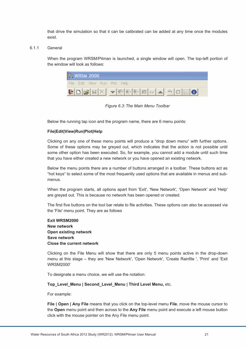
Water Resources of South Africa 2012 Study (WR2012): WRSM/Pitman User Manual 21
that drive the simulation so that it can be calibrated can be added at any time once the modules exist.
6.1.1 General
When the program WRSM/Pitman is launched, a single window will open. The top-left portion of the window will look as follows:
Figure 6.3: The Main Menu Toolbar
Below the running tap icon and the program name, there are 6 menu points:
File|Edit |View|Run|Plot|Help
Clicking on any one of these menu points will produce a “drop down menu“ with further options. Some of these options may be greyed out, which indicates that the action is not possible until some other option has been executed. So, for example, you cannot add a module until such time that you have either created a new network or you have opened an existing network.
Below the menu points there are a number of buttons arranged in a toolbar. These buttons act as “hot keys“ to select some of the most frequently used options that are available in menus and sub-menus.
When the program starts, all options apart from 'Exit', 'New Network', 'Open Network' and 'Help' are greyed out. This is because no network has been opened or created.
The first five buttons on the tool bar relate to file activities. These options can also be accessed via the 'File' menu point. They are as follows
Exit WRSM2000 New network Open existing network Save network Close the current network
Clicking on the File Menu will show that there are only 5 menu points active in the drop-down menu at this stage – they are 'New Network', 'Open Network', 'Create Rainfile ', 'Print’ and 'Exit WRSM2000'
To designate a menu choice, we will use the notation:
Top_Level_Menu | Second_Level_Menu | Third Level Menu, etc.
For example:
File | Open | Any File means that you click on the top-level menu File, move the mouse cursor to the Open menu point and then across to the Any File menu point and execute a left mouse button click with the mouse pointer on the Any File menu point.

Water Resources of South Africa 2012 Study (WR2012): WRSM/Pitman User Manual 22
Certain dialogs have tabbed sub-dialogs. For the operation to reach a tabbed sub-dialog, we will use the notation:
Top_Level_Menu | Second_Level_Menu [ | ... ] > Tab Name
For example:
Edit | Runoff Modules > General means that you click on the top level menu Edit, move the mouse cursor to the Runoff Modules menu point and execute a left-click on that item. When the dialog opens, and the tabbed dialog that is exposed is not the General tab, you should click on the General tab to get to the dialog that is indicated.
The term 'Pressing a button' means that you move the mouse cursor over the designated button and execute a left mouse button click while the mouse pointer is on the specified button.
To view a short description of a button in the toolbar, simply place the mouse cursor over the button in question. After a second, a short description of the action of the button will appear in a 'speech bubble'
6.1.2 Creating a new network
When you press the 'new' button or you choose the File | New Network menu point, the following dialog will appear:
Figure 6.4: The New Network dialog
In this dialog, you can specify:
The “Network Name”. This is the 3 character network code that will be used to name all the data files that you will be creating for this network. In this discussion, we will use the network code H1.
The “Data Folder” is the folder in which the program will create the different data files that will be created during the operation of the program, such as the Network file, Module data files, Rainfiles, Flows files, etc.
The “Result Folder” is the folder in which the result files will be places. Result files include such files as the error file and the summary file as well as the simulated flows that are generated by the program (see later).
To select either the Data Folder or the Result folder, you may click on the button marked ... to the right of the input field. This is the seek button and clicking on it will call up the standard Windows

Water Resources of South Africa 2012 Study (WR2012): WRSM/Pitman User Manual 23
Folder selection dialog. The seek button appears in all dialogs that require the input of a file name. Where a file is required, the standard Windows File selection dialog is opened.
Figure 6.5: The Dialog to Choose a Folder
To change the drive on which the folder is (or should be created) you can change the drive letter in the bottom-most drop-down list-box.
By selecting a folder in this dialog and either double clicking on it or pressing the OK button, this data is transferred automatically into the input field of the previous dialog. A new folder can be created by specifying its name in the folder selection dialog, in this case, by adding, for example \H1 behind the path name C:\WRSM2000. If the folder that you have selected does not exist, you will be asked whether you wish to create the directory:
Figure 6.6: The Create Directory (Create Folder) dialog
The result folder can be set by the same mechanism. The Data Folder and the Result Folder may be separate folders but they do not have to be – you may prefer to write the data and the results to the same folder.
In the dialog to create a new network (Error! Reference source not found.), you can also set the Simulation start and the Simulation end years. These years specify the time period for which the simulation will be run. Once these years are set, and the OK button is pressed, this range is valid for the current run of this network.
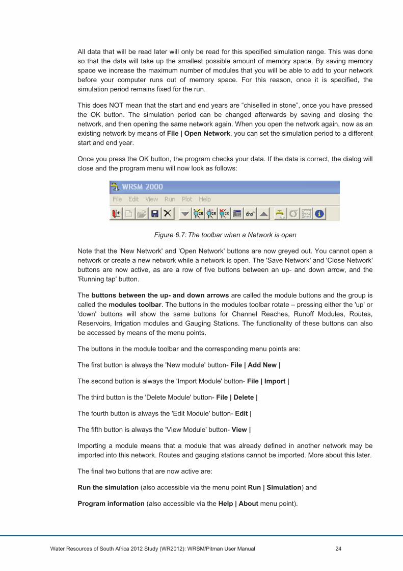
Water Resources of South Africa 2012 Study (WR2012): WRSM/Pitman User Manual 24
All data that will be read later will only be read for this specified simulation range. This was done so that the data will take up the smallest possible amount of memory space. By saving memory space we increase the maximum number of modules that you will be able to add to your network before your computer runs out of memory space. For this reason, once it is specified, the simulation period remains fixed for the run.
This does NOT mean that the start and end years are “chiselled in stone”, once you have pressed the OK button. The simulation period can be changed afterwards by saving and closing the network, and then opening the same network again. When you open the network again, now as an existing network by means of File | Open Network, you can set the simulation period to a different start and end year.
Once you press the OK button, the program checks your data. If the data is correct, the dialog will close and the program menu will now look as follows:
Figure 6.7: The toolbar when a Network is open
Note that the 'New Network' and 'Open Network' buttons are now greyed out. You cannot open a network or create a new network while a network is open. The 'Save Network' and 'Close Network' buttons are now active, as are a row of five buttons between an up- and down arrow, and the 'Running tap' button.
The buttons between the up- and down arrows are called the module buttons and the group is called the modules toolbar. The buttons in the modules toolbar rotate – pressing either the 'up' or 'down' buttons will show the same buttons for Channel Reaches, Runoff Modules, Routes, Reservoirs, Irrigation modules and Gauging Stations. The functionality of these buttons can also be accessed by means of the menu points.
The buttons in the module toolbar and the corresponding menu points are:
The first button is always the 'New module' button - File | Add New |
The second button is always the 'Import Module' button- File | Import |
The third button is the 'Delete Module' button - File | Delete |
The fourth button is always the 'Edit Module' button - Edit |
The fifth button is always the 'View Module' button - View |
Importing a module means that a module that was already defined in another network may be imported into this network. Routes and gauging stations cannot be imported. More about this later.
The final two buttons that are now active are:
Run the simulation (also accessible via the menu point Run | Simulation) and
Program information (also accessible via the Help | About menu point).

Water Resources of South Africa 2012 Study (WR2012): WRSM/Pitman User Manual 25
At the bottom of the program window, the name of the network that is currently loaded and the current state of activity of the program is shown in the status bar:
Figure 6.8: The status bar at the bottom of the main program window
Ready means that the program awaits your input.
Pressing the 'Run simulation' button or choosing the 'Run | Simulation' menu option to run the simulation will not bring much, since there are no modules in the network yet.
We first need to add modules to the network.
6.1.3 Adding a Runoff Module
A new runoff module can be added to a network by either rotating the module toolbar to RU and pressing the 'New' button, or by selecting the File | Add New | Runoff Module menu point.
The following dialog will be shown on the screen:
Figure 6.9: Creating a new Runoff Module
The Suggested Module number is a suggestion only. You may choose any number – as long as it is greater than 0 and less than 9999. The only proviso is that a Runoff Module with this number does not yet exist in the current network. The suggested module number will always be 1 larger than the last Runoff Module that was created. If a network contains many runoff modules and the next suggested number would be greater than 9999, the program will automatically scan through the list of Runoff Modules in the network to find the lowest unused module number that it can use.
During the cause of creating and deleting different modules, gaps may be created in the numbering. This is acceptable. You may, for example have created 7 Runoff Modules numbered 1 to 7 in a network, and then deleted the Runoff Module with the number 2. If you now add a new Runoff Module, the suggested module number will be 8 since the highest number for any of the existing Runoff Modules is 7 at this stage. Since you know that there is no runoff module with the number 2 (a fact that you can check with 'View' (see later)), you may change the suggested module number to the number 2.
Should you make a mistake, i.e. enter a number for a module that already exists in the network, the program will alert you to that, since duplicate module numbers are not allowed.
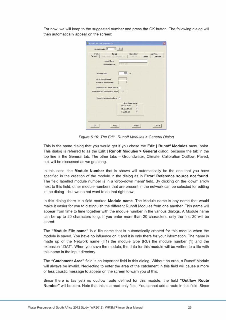
Water Resources of South Africa 2012 Study (WR2012): WRSM/Pitman User Manual 26
For now, we will keep to the suggested number and press the OK button. The following dialog will then automatically appear on the screen:
Figure 6.10: The Edit | Runoff Modules > General Dialog
This is the same dialog that you would get if you chose the Edit | Runoff Modules menu point. This dialog is referred to as the Edit | Runoff Modules > General dialog, because the tab in the top line is the General tab. The other tabs – Groundwater, Climate, Calibration Outflow, Paved, etc. will be discussed as we go along.
In this case, the Module Number that is shown will automatically be the one that you have specified in the creation of the module in the dialog as in Error! Reference source not found. The field labelled module number is in a 'drop-down menu' field. By clicking on the 'down' arrow next to this field, other module numbers that are present in the network can be selected for editing in the dialog – but we do not want to do that right now.
In this dialog there is a field marked Module name. The Module name is any name that would make it easier for you to distinguish the different Runoff Modules from one another. This name will appear from time to time together with the module number in the various dialogs. A Module name can be up to 20 characters long. If you enter more than 20 characters, only the first 20 will be stored.
The “Module File name” is a file name that is automatically created for this module when the module is saved. You have no influence on it and it is only there for your information. The name is made up of the Network name (H1) the module type (RU) the module number (1) and the extension “.DAT”. When you save the module, the data for this module will be written to a file with this name in the input directory.
The “Catchment Area” field is an important field in this dialog. Without an area, a Runoff Module will always be invalid. Neglecting to enter the area of the catchment in this field will cause a more or less caustic message to appear on the screen to warn you of this.
Since there is (as yet) no outflow route defined for this module, the field “Outflow Route Number” will be zero. Note that this is a read-only field. You cannot add a route in this field. Since
Water Resources of South Africa 2012 Study (WR2012): WRSM/Pitman User Manual 27
a route has a beginning and end point it is defined as a separate unit, but more about that later (under Adding Routes).
As there are no outflow routes defined for this Module, the “Number of Outflow Routes” is also still 0. Again: we cannot create outflow routes within the Runoff Module – this will be done later.
The check-box marked “This module is a Parent module” is unchecked when you create a new Runoff Module. This has to do with the Parent/Child configuration for Stream Flow Reduction (SFR) areas and will be discussed in more detail later.
Similarly, the field marked “This module is a Child module to RU” will contain a 0, since this particular module is not a Child to any other module. This will be discussed in more detail later and we can ignore it for now.
By default, the checkbox marked “Simulate Naturalised outflows” is unchecked when a new module is created. When this checkbox is checked (i.e. has a tick mark in it), the module will ignore all man-made module data such as Paved areas, Afforestation and Alien Vegetation and so produce naturalised outflows for the catchment. This will only apply to this specific Runoff module.
At present, there are three groundwater models available in the Runoff Module, the Pitman model, the Hughes model and the Sami Model. By default, and for backwards compatibility, all new Runoff modules suggest that the Pitman Groundwater model is used. You may change this by clicking on the radio button for the Hughes model or the Sami Model. Note that the Edit | Runoff Modules > Hughes GW and the Edit | Runoff Modules > Sami GW tabs are greyed out when the Pitman Groundwater model is used. This is because there is no data in those dialogs that is relevant to the Pitman Groundwater model. When the radio button set to the Hughes Groundwater Model or the Sami Groundwater Model, the dialog tab does not change immediately. It is only when you press the Apply button, that the Edit | Runoff Modules > Hughes GW or the Edit | Runoff Modules > Sami GW tab will be activated.
There are four buttons at the base of the dialog:
OK- remember all the changes, check the data and close the dialog
Apply- remember all the changes, but don't close the dialog
Check- remember all the changes and check whether this module is valid
Cancel- close the dialog, don't remember the changes
Note that pressing Cancel after having pressed Apply does not undo all the changes but merely those that were made since the last time the Apply button was pressed.
After entering the name of the catchment as 'Runoff 1' and the area as '371.0' km² and changing the groundwater model to the Hughes Groundwater Model, we press the OK button. Immediately, we are rewarded with our first error message:

Water Resources of South Africa 2012 Study (WR2012): WRSM/Pitman User Manual 28
Figure 6.11: The Missing MAP dialog
Without having been asked, the program automatically checked the data so far and found that the Mean Annual Precipitation was not set for this module. You will note that the Edit Runoff dialog also did not close.
Since M.A.P. is a feature of Climate, we click on the Climate tab to get the following dialog:
Figure 6.12: The Edit | Runoff Modules > Climate
We add the MAP of 750 mm and press OK again.
Again we get a message:
Figure 6.13: The Missing Rainfile Dialog

Water Resources of South Africa 2012 Study (WR2012): WRSM/Pitman User Manual 29
This is more serious: we do not have a Rainfile.
After pressing the OK button on the Runoff Module Check dialog, we press the Cancel button in the Edit Runoff Module parameters dialog. This closes the dialog, and we are back at the previous dialog.
Figure 6.14: The Create New Runoff Module dialog (2)
The model is ready to add the next Runoff Module. We can see that because the next Suggested Module number is number 2.
We don't want any more Runoff Modules at this stage, and therefore we either press the Cancel button or the Close dialog cross at the top right.
6.1.4 Creating a Rainfile
6.1.4.1 Creating a Rainfile from Weather Bureau rainfall files
A Rainfile is a file that contains the monthly rainfall expressed as a percentage of the Mean Annual Precipitation. It is a catchment based file that is created from one or more station rainfall files that cover that catchment. It is wise to choose station rainfall files that cover both the geographical area well and also cover the record period adequately. The station rainfall files are obtained via the WR2012 website, DWS Rainfall IMS model (called WRMF) or the Weather Bureau. An example of the name of one is 0079504.MP where the 0079504 describes its position (refer to the WR90 study mapbooks). The catchment based rainfall file can be called anything but the normal convention is to give it the designation “RAN”, e.g. B41.RAN .
Within WRSM/Pitman, there is an option to create such a file from weather bureau rainfall files by selecting the option File | Create Rainfile. Selecting this option will result in a dialog box as shown below. This option takes the place of the DOS program HDYP09.
Figure 6.15: The File | Create Rainfile Dialog

Water Resources of South Africa 2012 Study (WR2012): WRSM/Pitman User Manual 30
To create a Rainfile, you will be prompted for the “Gauge Code”. This is the code that will appear at the start of each row in the Rainfile to be created – it is the name of the Gauge that you create. The model will, however, accept any code.
The “Time Period” is the period for which the Rainfile must be generated. This period must cover at least the period for which you wish to run the simulation.
The “Rainfile name” is the name of the Rainfile to be created. As described on the previous page, this is the catchment based rainfall file name and can be anything but the normal convention is “*.RAN” where the * describes the catchment, e.g. “B41.RAN”. This is the datafile that will be required in various modules, particularly the runoff module.
The “Report file” is the name of a file into which relevant data is written when the Rainfile is created. Any name can be entered or selected but the normal convention is “*.DOC”, for example “B41.DOC”.
A “Raingauge file” is a Weather Bureau rainfall file or a file from the Rainfall IMS. These datafiles normally have the form (for example) “0079504.MP” where the number refers to the geographical position (See the WR90 study mapbooks).
Whenever a file needs to be chosen, you can do this by means of a file selection dialog. To open the file selection dialog, you click on the search button (the one with the 3 dots) next to the relevant input field.
When a Weather Bureau “Raingauge file” is selected, clicking on the Add button will transfer the file name to the “Raingauge Files to Use” list on the right hand side of the dialog. Selecting and adding a file to this list can be repeated until all the necessary rain gauge files are in this list.
If you make a mistake, a file can be removed from the “Raingauge Files to use” list by first clicking on the file to be removed and then either clicking on the Delete button. The time series file (the Rainfile) is created once you click on the Calculate button. This will create the “Rainfile name” datafile and “Report file“ datafile. If the calculation is successful, the words “rainfile was created successfully” will appear in a pop-up window.
Once the time series is calculated, you can plot the geographic and temporal distribution graphs. The type of plot to be produced is specified by selecting one of the radio buttons Geographic Plot or Temporal Distribution Plot. Clearly, None means no plot. You can display the plots on the screen by pressing the Screen button, or send the plot to your printer by pressing the Printer button, provided that you specified a plot.
The graph of the geographic distribution shows the relative geographic positions of the raingauges that were used, and the temporal distribution graph shows the number of raingauges that were used to determine the time series for a given year.
Two new graphs have been added, namely: a catchment rainfall massplot and a catchment rainfall CUSUM plot. The catchment rainfall massplot is obtained by taking the cumulative rainfall (as percentage of MAP) and plotting against time. It is used to ascertain if all the individual rainfall stations are providing an acceptable catchment rainfall datafile. This is the case if one gets a reasonably straight line on the massplot (which is in percentage of MAP). Small changes in slope are indicative of sustained periods of low (flatter slope) or high (steeper slope) rainfall. However, if there is an appreciable change in slope of the line, then it is likely that either the choice of individual rainfall stations is inadequate or that there are inaccuracies in one or more of the rainfall records. One should then look at individual massplots using say the WRIMS model (which has this

Water Resources of South Africa 2012 Study (WR2012): WRSM/Pitman User Manual 31
option) to establish where the inaccuracies lie. An example of the catchment rainfall massplot is shown in Figure 6.16.
Figure 6.16: The Catchment Rainfall Massplot
The second new graph is the CUSUM plot. The difference between cumulative rainfall less the cumulative mean percentage (taken to be 100%) is plotted against time, which results in a more sensitive picture of the variation in rainfall than that shown in a massplot. It should be noted that unlike the streamflow CUSUM plot, the catchment rainfall CUSUM plot will normally not end at exactly zero on the y-axis. This is because the average of the mean annual average of the catchment rainfall datafile is normally close to but not equal to 100%. This happens because one usually has to select rainfall records covering different periods in order to obtain an acceptable coverage over the full period of simulation. In the example below the mean annual average is 100.26% (which one obtains from the document output datafile) which ties in with the graph being about +15% (in the last year) over 61 years which is 0.25. The month before the start year has been set to zero as for the streamflow massplot. Years in the positive territory of the graph would indicate above average rainfall and vice versa. A normal catchment based rainfall datafile should show more or less even positive and negative territories. A catchment based drought event would appear as a prolonged downwards curve (such as from about 1938 to 1951 and 1960 to 1965 in Figure 6.17 below). If the final point is a lot higher or lower than 0 and/or the positive and negative territories are totally out of balance, this would probably indicate that more individual stations need to be selected and/or there are some inaccuracies in one or more of the individual rainfall records.
The CUSUM plot is shown in Figure 6.17
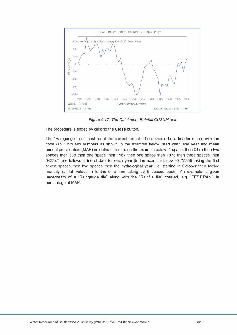
Water Resources of South Africa 2012 Study (WR2012): WRSM/Pitman User Manual 32
Figure 6.17: The Catchment Rainfall CUSUM plot
The procedure is ended by clicking the Close button.
The “Raingauge files” must be of the correct format. There should be a header record with the code (split into two numbers as shown in the example below, start year, end year and mean annual precipitation (MAP) in tenths of a mm. (in the example below -1 space, then 0475 then two spaces then 338 then one space then 1967 then one space then 1973 then three spaces then 6433).There follows a line of data for each year (in the example below -0475338 taking the first seven spaces then two spaces then the hydrological year, i.e. starting in October then twelve monthly rainfall values in tenths of a mm taking up 5 spaces each). An example is given underneath of a “Raingauge file” along with the “Rainfile file” created, e.g. “TEST.RAN” .in percentage of MAP.
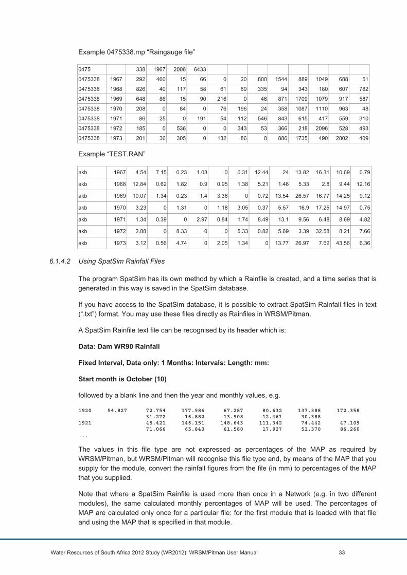
Water Resources of South Africa 2012 Study (WR2012): WRSM/Pitman User Manual 33
Example 0475338.mp “Raingauge file”
0475 338 1967 2006 6433
0475338 1967 292 460 15 66 0 20 800 1544 889 1049 688 51
0475338 1968 826 40 117 58 61 89 335 94 343 180 607 782
0475338 1969 648 86 15 90 216 0 46 871 1709 1079 917 587
0475338 1970 208 0 84 0 76 196 24 358 1087 1110 963 48
0475338 1971 86 25 0 191 54 112 546 843 615 417 559 310
0475338 1972 185 0 536 0 0 343 53 366 218 2096 528 493
0475338 1973 201 36 305 0 132 86 0 886 1735 490 2802 409
Example “TEST.RAN”
akb 1967 4.54 7.15 0.23 1.03 0 0.31 12.44 24 13.82 16.31 10.69 0.79
akb 1968 12.84 0.62 1.82 0.9 0.95 1.38 5.21 1.46 5.33 2.8 9.44 12.16
akb 1969 10.07 1.34 0.23 1.4 3.36 0 0.72 13.54 26.57 16.77 14.25 9.12
akb 1970 3.23 0 1.31 0 1.18 3.05 0.37 5.57 16.9 17.25 14.97 0.75
akb 1971 1.34 0.39 0 2.97 0.84 1.74 8.49 13.1 9.56 6.48 8.69 4.82
akb 1972 2.88 0 8.33 0 0 5.33 0.82 5.69 3.39 32.58 8.21 7.66
akb 1973 3.12 0.56 4.74 0 2.05 1.34 0 13.77 26.97 7.62 43.56 6.36
6.1.4.2 Using SpatSim Rainfall Files
The program SpatSim has its own method by which a Rainfile is created, and a time series that is generated in this way is saved in the SpatSim database.
If you have access to the SpatSim database, it is possible to extract SpatSim Rainfall files in text (“.txt”) format. You may use these files directly as Rainfiles in WRSM/Pitman.
A SpatSim Rainfile text file can be recognised by its header which is:
Data: Dam WR90 Rainfall
Fixed Interval, Data only: 1 Months: Intervals: Length: mm:
Start month is October (10)
followed by a blank line and then the year and monthly values, e.g.
1920 54.827 72.754 177.986 67.287 80.632 137.388 172.358 31.272 16.882 13.908 12.461 30.388
1921 45.421 146.151 148.643 111.342 74.442 47.109 71.066 65.840 61.580 17.927 51.370 86.260
...
The values in this file type are not expressed as percentages of the MAP as required by WRSM/Pitman, but WRSM/Pitman will recognise this file type and, by means of the MAP that you supply for the module, convert the rainfall figures from the file (in mm) to percentages of the MAP that you supplied.
Note that where a SpatSim Rainfile is used more than once in a Network (e.g. in two different modules), the same calculated monthly percentages of MAP will be used. The percentages of MAP are calculated only once for a particular file: for the first module that is loaded with that file and using the MAP that is specified in that module.

Water Resources of South Africa 2012 Study (WR2012): WRSM/Pitman User Manual 34
Subsequently, WRSM/Pitman will determine the rainfall (in mm) for a particular month for a particular module with this file by means of:
Monthly_rainfall = Monthly_percentage_of_MAP / 100. * MAP_of_the_module.
Example:
In the data above, the precipitation was 54.827 mm in October of the year 1920. If the MAP in the first module in which the Rainfile was used was set to 900 mm. it follows that the Monthly_percentage_of_MAP for October, 1920 would have been calculated as 6.09189.
If we now use the same Rainfile in a second module and specify an MAP of 750 mm for that module, the precipitation for that module will be calculated as 45.689 mm for October of 1920. This is not the 54.827 mm of the original file.
WRSM/Pitman saves the MAP that was used to make the conversion. It will warn you when a subsequent Module uses an MAP that is not the same as the MAP that was used to make the conversion.
To avoid this effect the obvious solution would be to set the MAPs in the two modules to identical values. To get the actual figures from the same file at different MAPs, make a copy of the file and give it a different name. Use a file with a different name in each module, since a different file name will be treated as a different Rainfile.
6.1.5 Editing a Runoff Module.
By selecting the option Edit | Runoff Modules (or selecting the appropriate button from the rotating module toolbar), we once again open the Runoff Module Parameters dialog.
Figure 6.18: The Edit | Runoff Modules dialog
Note that the Module number is blank when we call up this dialog. Because we have not yet defined which module is to be edited, there is also no data in any of the fields of the dialog. The first thing to do, therefore, is to set the number of the Runoff Module that we want to edit.

Water Resources of South Africa 2012 Study (WR2012): WRSM/Pitman User Manual 35
By clicking on the down-arrow next to the Module Number drop down list box, the numbers of the Runoff Modules that are currently in the network are displayed. If you have a scroll mouse, simply clicking on the menu field and scrolling will also display the different Runoff Modules (and load the data). The two Arrow buttons next to the Module Number drop down list box can also be used to scroll backwards and forwards through the Runoff Modules in the current Network.
6.1.6 Editing a Runoff Module, Climate dialog
When we select Runoff Module 1, the data that we have entered already will automatically be placed in the dialog fields. We do not need to change anything in the Edit | Runoff Modules > General dialog and so we click on the Climate-tab to enter the name of the Rainfile that we created above in the appropriate field.
Again we can use the search file button next to the Rainfile input field to select the appropriate file name.
Figure 6.19: The Edit | Runoff Modules > Climate dialog
We now need to add the 12 Symons pan Evaporation values and (if necessary) change the SPan Factors for the different months. If we do not add the Evaporation values, the module check will tell us that 0 is a suspicious value for evaporation and that 12 of those were found.
Note: If Span factors are used, the default pan factors should be used as given in WR90, Appendix 3.3.1 (Catchment evaporation).
The Sami Groundwater model uses APan evaporation values and APan factors to determine the amount of evaporation from the groundwater zone. Unless the Sami groundwater model is used, the row (APan Factors) is unimportant.
When you specify that the Sami model is to be used, the SPan evaporations are automatically converted to APan evaporations internally in the program as and when they are needed. You will not actually see any evidence of this, but you can rest assured that it will be done for you. The APan Factors are not so cut-and-dried, which is the reason for their presence in this dialog. Initial values for the Apan factors will also be calculated for you. To see this feature of the program, fill in
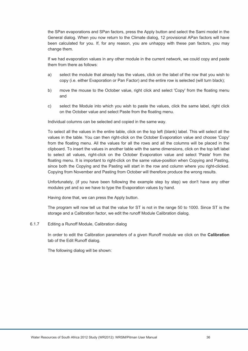
Water Resources of South Africa 2012 Study (WR2012): WRSM/Pitman User Manual 36
the SPan evaporations and SPan factors, press the Apply button and select the Sami model in the General dialog. When you now return to the Climate dialog, 12 provisional APan factors will have been calculated for you. If, for any reason, you are unhappy with these pan factors, you may change them.
If we had evaporation values in any other module in the current network, we could copy and paste them from there as follows:
a) select the module that already has the values, click on the label of the row that you wish to copy (i.e. either Evaporation or Pan Factor) and the entire row is selected (will turn black);
b) move the mouse to the October value, right click and select 'Copy' from the floating menu and
c) select the Module into which you wish to paste the values, click the same label, right click on the October value and select Paste from the floating menu.
Individual columns can be selected and copied in the same way.
To select all the values in the entire table, click on the top left (blank) label. This will select all the values in the table. You can then right-click on the October Evaporation value and choose 'Copy' from the floating menu. All the values for all the rows and all the columns will be placed in the clipboard. To insert the values in another table with the same dimensions, click on the top left label to select all values, right-click on the October Evaporation value and select 'Paste' from the floating menu. It is important to right-click on the same value-position when Copying and Pasting, since both the Copying and the Pasting will start in the row and column where you right-clicked. Copying from November and Pasting from October will therefore produce the wrong results.
Unfortunately, (if you have been following the example step by step) we don't have any other modules yet and so we have to type the Evaporation values by hand.
Having done that, we can press the Apply button.
The program will now tell us that the value for ST is not in the range 50 to 1000. Since ST is the storage and a Calibration factor, we edit the runoff Module Calibration dialog.
6.1.7 Editing a Runoff Module, Calibration dialog
In order to edit the Calibration parameters of a given Runoff module we click on the Calibration tab of the Edit Runoff dialog.
The following dialog will be shown:

Water Resources of South Africa 2012 Study (WR2012): WRSM/Pitman User Manual 37
Figure 6.20: The Edit | Runoff Modules > Calibration dialog
The Soil Moisture capacity can be set to 100 mm as a first approximation.
A note about the colour scheme. The user will notice that some of the input fields in certain of the dialogs have a light blue, others a pink and others a white background. The pink calibration parameters should not be changed, the blue can be changed if the data is available and the white are usually changed.
Since the Calibration dialog deals only with calibration parameters and all of these can be used to improve your calibration, all the active parameters will have a light blue background. This is not the case in the Hughes GW and the Sami GW dialogs. In these dialogs, some parameters will have a light blue background and others will have a white background. The light blue parameters are the ones that can be changed to improve your calibration, whereas the others are either 'set-once-and-forget' or 'don't-change-this-from-the-default'. We will point those out later in this document.
Note that these calibration parameters are for a catchment that uses the Hughes Groundwater Model as we specified in the Edit | Runoff Modules > General dialog. We know that this module will use the Hughes Groundwater Model because the fields GPOW, HGGW, TLGMax and GWSLinit are active, and the fields GW and GL are inactive.
The fields for GW and GL are inactive because they apply to the Pitman Groundwater Model. Had we selected the Pitman Groundwater Model in the Edit | Runoff Modules > General dialog, these fields would be active.
As can be seen from (Hughes et al., 2004), the value for the variable SL was usually set at 0 in the Pitman Groundwater Model. Hughes therefore redefined this variable in his discussion.
In the implementation of this idea in WRSM/Pitman it was decided not to use this redefinition and to use separate variables for three reasons:
a) the two variables describe very different physical characteristics;

Water Resources of South Africa 2012 Study (WR2012): WRSM/Pitman User Manual 38
b) it is possible to change the selected Groundwater Model by simply changing the choice of model in the Edit | Runoff Modules > General dialog. The three models (and their corresponding variable values) must therefore coexist side by side in the same program and
c) with the advent of the Parent/Child scenario in Stream Flow Reduction (SFR) elements, the value of SL is no longer 'usually 0'.
The same reasoning applies to the parameter GW that is used in the Pitman Groundwater Model. The variable GW that is described in (Hughes et al., 2004) is implemented as HGGW in WRSM/Pitman.
In the Hughes Groundwater Model there is no need for a ground water lag (parameter GL) because the Hughes Groundwater Model acts as a routing reservoir. For this reason, the GL field is blanked out.
For a discussion of the parameters GPOW, HGSL, HGGW, TLGMax and GWSLinit you are referred to (Hughes et al., 2004). In this report, there are also tips on the values for the other parameters that pertain to the Hughes Groundwater Model. A value for GPOW is also required in the Sami model, and therefore this field will be active if you select the Sami Groundwater Model. Certain values for the Hughes parameters can also be obtained from the Conrad database (which covers all quaternaries in South Africa). Use can also be made of the WSAM database and the DWAF GRA II study Reports.
For a detailed discussion of the other parameters you are referred to HRU report (Pitman, 1973). See also WRSM/Pitman Theory (Stewart Scott, 2006)
A special note about the “Forest Factor” (FF). In previous versions of WRSM/Pitman, the Forest Factor was always 1.00 and was therefore never even mentioned. Now, with the advent of the Parent/Child configuration, this forest factor has been activated. You will notice that no matter what you do, the field for Forest Factor will always be read-only, and you will never be able to change this parameter yourself. This is not an error. The value for the Forest Factor may change when you use the Parent/Child configuration for Stream Flow Reduction elements, but WRSM/Pitman will adjust FF automatically when it reduces the outflows for the Child SFR. This value will therefore be shown, but you have no direct influence on it. The FF parameter field is therefore merely an information field.
If you do not know the approximate values for the parameters please refer to the Water Research Commission WR90 reports (Midgley et al., 1990) for the region in which you are working.
When you have entered the parameter values, they can be saved by pressing the Apply button. This will also execute a check on the values to see whether they are within reasonable limits.
You may swap between the different dialogs by clicking on the appropriate tab and change the values in the fields, but these changes are only registered once you press the OK button or the Apply button.
Should you change from one Runoff Module to another by changing the Module Number by any of the means described above, any changes that were made after the last time the Apply button was pressed, will be lost. It is therefore important to press the Apply button before changing from one Runoff Module (or indeed any other module) to another while editing the modules.

Water Resources of South Africa 2012 Study (WR2012): WRSM/Pitman User Manual 39
Calibration parameters – making changes to selected multiple runoff modules
If you wish to have exactly the same set of calibration parameters in all or some of the runoff modules in your network, this can be done using the “Apply to Selected Runoff Modules” button. Selecting this button will bring up the following window shown in Figure 6.19. The user can either select all runoff modules in the network by pressing the “Add to All” button or select only specific runoff modules by pressing the down arrow in the “Runoff Module” box and progressively building up the “Runoff Modules in Group” window using the “Add to list” button each time. Runoff modules can be de-selected using the “Remove from list” button or to remove the whole lot by using the “Remove All” button. This works in a very similar way to selecting rainfall stations for a catchment rainfall datafile. Once the user is happy with the selected runoff modules in the “Runoff Modules in group” box, the “Apply to Selected Runoff Modules” button should be pressed. Finally press the “OK” button to exit this window. This will take the existing set of calibration parameters and copy them to all the runoff modules selected. This is particularly useful in catchments where there is very little variation in hydrological conditions from one quaternary catchment to another such as the very dry Lower Orange WMA for example.
Figure 6.21: The Select Runoff Modules for Applying Calibration Parameters Dialog
6.1.7.1 Changing from Pitman to Sami or Hughes groundwater methods
One should also realise that there may be up to three different calibration parameter sets in a given Runoff Module: one set for each Groundwater Model (Pitman, Sami and Hughes). This was done because the different groundwater models tend to calibrate at different values for a given parameter. It means that a common variable such as ST may (for example) be 100 in the Pitman Groundwater Model, 130 in the Hughes Model and 110 in the Sami Model for the best calibration. Therefore if the user sets up calibration parameters for the Pitman method first (as advised) and then switches to the Sami or the Hughes method, the relevant calibration parameters for the Pitman method must be copied to the calibration parameters for the Sami method.
When switching from the Pitman model to the Sami model there should not be much difference between the simulated flows – this is particularly the case where default parameters are used for the Sami model. A notable exception to this result will occur when the parameters GW and GL are

Water Resources of South Africa 2012 Study (WR2012): WRSM/Pitman User Manual 40
used in the Pitman model (i.e. they are not set to the default values of zero). These two parameters govern the groundwater function of the Pitman model and are accordingly switched off when the Sami model is selected.
An important feature in the Pitman model is the way it handles "excess" water that cannot be absorbed by the soil – a situation that can occur in months of high rainfall. This excess is split into groundwater and surface water according to the ratio GW/FT. The outcome is that a proportion of the excess water is subject to a lag of GL, which augments baseflow following high rainfall. When one switches to the Sami model (when GW and GL are re-set to zero) all the excess water becomes surface runoff – subject to a lag TL (where TL << GL), with the result that months of high runoff will become higher. In such cases one would need to increase ST in order to reduce the peak months and render them comparable to the flows generated by the Pitman model.
We now describe the Hughes Groundwater Model Parameters which are accessed by means of either the Edit | Runoff Modules > Hughes GW or the Edit | Runoff Modules > Sami GW tabbed dialog.
6.1.8 Editing a Runoff Module, Hughes GW dialog
It is strongly recommended that one first uses the tried and tested Pitman method when first calibrating. Once a reasonable calibration has been achieved, the Hughes (or Sami) method can be activated and the calibration fine-tuned.
The Hughes GW dialog of the Edit Runoff Module dialog will only be available (and indeed necessary) if you have specified that the Runoff Module in question is to use the Hughes Groundwater Model. This is done in the Edit | Runoff Modules > General dialog for the specific Runoff Module. If you specified the Pitman Groundwater Model or the Sami Groundwater Model there, the Hughes GW dialog is not necessary and therefore the tab is greyed out.
The Edit | Runoff Modules > Hughes GW dialog is concerned mainly with the physical characteristics of the catchment that affect Groundwater for the Hughes Model.
Figure 6.22: The Edit | Runoff Module > Groundwater dialog

Water Resources of South Africa 2012 Study (WR2012): WRSM/Pitman User Manual 41
Note that there are only two parameter fields that are used to improve the calibration of the groundwater simulation in the Hughes model, namely: transmissivity and rest water level. Other calibration parameters are to be found in the Edit/Runoff Module > Calibration dialog. The other parameters in the Edit/Runoff Module/Hughes GW dialog should be set once and then left constant for the calibration.
Groundwater is a regional phenomenon that does not necessarily follow the quaternary catchment boundaries that are used to determine surface runoff. For this reason, the final groundwater conditions in an upstream catchment can be of some significance. For this reason, you may specify one “Upstream Runoff Module to this Module” whose final groundwater state will influence the groundwater state of the current module. The upstream runoff module that is specified here must, of course, also be simulated using the Hughes Groundwater Model.
If a module is to be defined as being 'upstream' to another module, it follows that the order in which the modules are solved is important. This will be discussed in greater detail later.
There is also a difference between the Upstream Runoff Module for groundwater and the inflows to the Runoff Module. This and how the two groundwater models handle the inflows are discussed in greater detail in the next section.
As can be seen from the theoretical discussion of the Hughes Groundwater Model, a (sub) catchment that is represented by a Runoff Module is first divided into a number of drainage elements, each with a pair of drainage slopes – one on either side of the channel. The number of drainage reaches in a catchment is used to determine the drainage density of the catchment by means of the formula:
Drainage Density = Number of branches / square root of the catchment area
For further information, refer to (Hughes et al., 2004) in the section Geometry of the ground water store, Figure 2.
From the drainage density, the drainage slope length and width is determined. As a user, you only have to count the number of drainage channels in the catchment which is entered into the field “Drainage by means of ___ reaches”. Changing this value can be used to set the drainage density to any acceptable figure.
Changing the number of reaches and pressing the Apply button will recalculate the drainage density, the number of drainage slopes, the drainage slope length and the drainage slope width. By changing this figure, a desired drainage density can be set.
If on the other hand, you already know the drainage density of a given catchment, it is also possible to enter this value directly into the dialog. To enter a specific drainage density, you must first disable the field “Drainage by means of ___ reaches”. You disable this field by first clicking on the tick mark that is placed just before the dialog field so that the tick mark disappears, and then pressing the Apply button. When you press the Apply button, the “Drainage by means of” field will be deactivated. At the same time, the “Drainage Density” field will be activated. You can now enter the drainage density that you have. By pressing the Apply button again, the parameters for number of drainage slopes and the drainage slope lengths and widths will be calculated, based on the drainage density that you supplied. The latter fields will never be activated – they are there only for your information. A default of 0.4 can be used if the user has no information on this.

Water Resources of South Africa 2012 Study (WR2012): WRSM/Pitman User Manual 42
To activate the “Drainage by means of” field again, you click on the checkbox again so that the tick mark re-appears. After you press the Apply button again, you can enter the number of reaches again to have the model calculate the drainage density for you.
A drainage slope is conceptually split into two zones, namely: the Riparian zone and the Upper zone. By definition, the Riparian zone constitutes 40% of the drainage slope. It is possible to change this ratio in WRSM/Pitman, but this is not recommended. This is meant for experimental purposes only.
The “Riparian Evaporation strip” is discussed in (Hughes et al., 2004) in the section Riparian losses to evapotranspiration. Hughes suggests using a value of 0.2%. This is given as a percentage of the riparian zone.
“Storativity and Transmissivity” are discussed in (Hughes et al., 2004) – in the section Parameter value estimation. The Conrad database can be used for data – refer to the “MEAN-SSATI” variable for storativity and the “MEAN-TRANS” variable for transmissivity. Hughes suggests taking a half of this value. Defaults of 0.001 and 10 m²/d have been given in the WRSM/Pitman model for storativity and transmissivity respectively.
“Restwater Level” is also discussed in this section. Note that the figure that is entered here must be a positive value. The Conrad database can be used for obtaining data – refer to the “MED-STHK” variable. A default of 20 m can be used.
“Annual Groundwater Abstractions” and the monthly distributions (as percentages of the total abstractions) for either or both the Riparian and Upper zones speak for themselves.
“GPOW” is discussed in (Hughes et al., 2004). Hughes suggests an initial value of 3 to begin calibration.
“HGSL” is discussed in (Hughes et al., 2004). Hughes suggests an initial value of 0.
“HGGW” is discussed in (Hughes et al., 2004). Hughes suggests the following calculation:
= Annual recharge * (0.65)GPOW 12
A default of 2 can be used
“TLGMax” is discussed in (Hughes et al., 2004). Hughes suggests an initial value of 2.
“Regional Groundwater GW gradient”. Hughes suggests the following calculation:
= 0.01 * (MEAN_SL_P)0.05 100
When the OK or Apply buttons are pressed, the data that you have entered will be checked. If the values are outside of the normal ranges, there will be messages to alert you to this. Note that the abstraction percentages will only be checked if abstractions were actually specified.
6.1.8.1 Runoff Module inflows and Upstream Modules for Groundwater – an aside.
Any route from upstream can be made an inflow route to a Runoff Module. The outflow from one catchment (or part of it) can therefore be routed through the next catchment.
or 0.01

Water Resources of South Africa 2012 Study (WR2012): WRSM/Pitman User Manual 43
The three Groundwater models handle such inflows in different ways. If the Runoff Module that receives the inflow uses the Pitman Groundwater Model or the Sami Groundwater model, there are no losses – what comes in via the inflow route goes out via the outflow route(s). Any runoff that is generated by a Runoff Module is added to the inflow.
If the Runoff Module uses the Hughes groundwater model, some of the inflow may be diverted to groundwater if the groundwater storage falls below a certain minimum. This means that the outflow to the Runoff Module could actually be less than what comes in. The reason for adding an inflow route in the first place was because the Hughes Model has the ability to take flow from the river channel that runs through the Runoff Module, if the storage in the riparian zone becomes too low.
The total loss to groundwater is limited to a the value of “TLGMax”, which is set in the Edit | Runoff Module > Calibration dialog. If “TLGMax” is 0, there will be no losses to Groundwater. If “TLGMax” is not 0, it means that there will be 'losses' to groundwater, and the outflow of a particular Runoff Module could, under certain conditions, be less than what was supplied via the inflow Route. As in the case of the Pitman and the Sami Groundwater Models, if any Runoff is actually generated by the Runoff Module, it is added to the (reduced) outflow again.
The user can add an inflow route to a Runoff Module in the same way as you do with every other Module – as described in the section Adding a Route.
Some may find the idea of an "Upstream Runoff Module” (for groundwater) and an "Inflow Route" confusing. This is understandable. In short, the two have nothing to do with one another.
In the Hughes Groundwater Model, the storage states in the groundwater zones (riparian and upper) can be passed on from one Runoff Module to the next.
Groundwater is a regional phenomenon that does not necessarily follow the quaternary catchment boundaries that surface water hydrologists habitually work with. Contrary to intuition, the Runoff Module directly upstream of a particular Runoff Module, the one that supplies the surface inflows, is therefore not necessarily the one that influences the groundwater storage, since the groundwater regions may cross the quaternary boundaries.
The flows in the inflow route to the Runoff Module have nothing to do with the storage states of groundwater in any of the upstream catchments since it is surface water, but the flow in the channel of the Runoff Module (supplied through the inflow route) may influence the groundwater storage of the riparian zone of the Runoff Module through which it flows.
6.1.9 Editing a Runoff Module, Sami GW dialog
The Sami GW dialog of the Edit Runoff Module dialog will only be accessible if you have specified that the Runoff Module in question is to use the Sami Groundwater Model. This is done in the Edit | Runoff Modules > General dialog for the specific Runoff Module. If you specified the Pitman Groundwater Model or the Hughes Groundwater model there, the Sami GW dialog is not necessary and therefore the tab will be greyed out.
The Edit | Runoff Modules > Sami GW dialog is concerned with the physical characteristics of the catchment that affect Groundwater for the Sami Model.
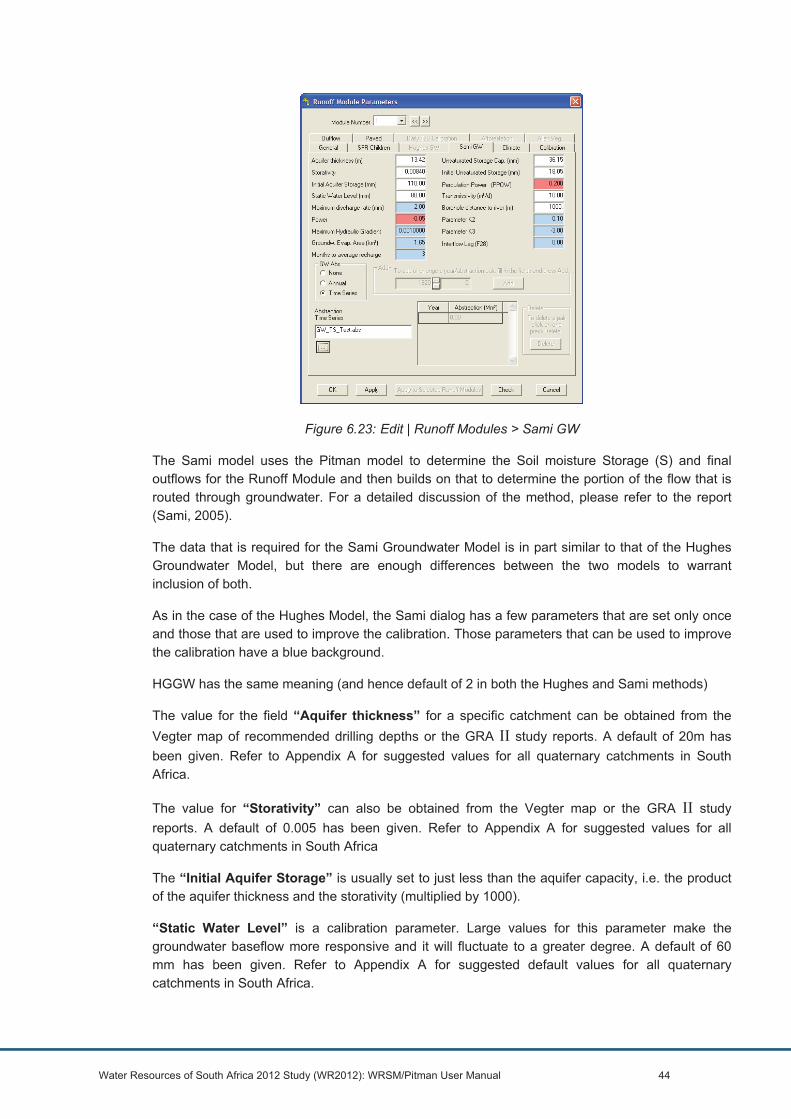
Water Resources of South Africa 2012 Study (WR2012): WRSM/Pitman User Manual 44
Figure 6.23: Edit | Runoff Modules > Sami GW
The Sami model uses the Pitman model to determine the Soil moisture Storage (S) and final outflows for the Runoff Module and then builds on that to determine the portion of the flow that is routed through groundwater. For a detailed discussion of the method, please refer to the report (Sami, 2005).
The data that is required for the Sami Groundwater Model is in part similar to that of the Hughes Groundwater Model, but there are enough differences between the two models to warrant inclusion of both.
As in the case of the Hughes Model, the Sami dialog has a few parameters that are set only once and those that are used to improve the calibration. Those parameters that can be used to improve the calibration have a blue background.
HGGW has the same meaning (and hence default of 2 in both the Hughes and Sami methods)
The value for the field “Aquifer thickness” for a specific catchment can be obtained from the Vegter map of recommended drilling depths or the GRA II study reports. A default of 20m has been given. Refer to Appendix A for suggested values for all quaternary catchments in South Africa.
The value for “Storativity” can also be obtained from the Vegter map or the GRA II study reports. A default of 0.005 has been given. Refer to Appendix A for suggested values for all quaternary catchments in South Africa
The “Initial Aquifer Storage” is usually set to just less than the aquifer capacity, i.e. the product of the aquifer thickness and the storativity (multiplied by 1000).
“Static Water Level” is a calibration parameter. Large values for this parameter make the groundwater baseflow more responsive and it will fluctuate to a greater degree. A default of 60 mm has been given. Refer to Appendix A for suggested default values for all quaternary catchments in South Africa.

Water Resources of South Africa 2012 Study (WR2012): WRSM/Pitman User Manual 45
Note: If the “Static Water Level” divided by the capacity (storativity * aquifer thickness * 1000) is greater than about 90% and the catchment area is very small (as could be the case with a child module for say afforestation), the streamflow could become unstable resulting in “******” showing for some months. In this case the aquifer cannot drain properly. Sami has calculated revised “Static Water Level” values for every quaternary catchment (see Appendix A for SWL Sami revised 2014). If this problem occurs the user should also consider the storativity values as very low storativity values may lead to unrealistically low aquifer capacities. In general aquifer capacity should not be less than 20 mm. Very low values may lead to very low aquifer volumes, resulting in the aquifer being unable to accept recharge and unrealistically high storm runoff values.
Pushing up the SWL is, however, the only way to make baseflow intermittent for ephemeral systems with some baseflow.
Please note that Appendix A contains default data and some values may not be that realistic. It is, however, the only national groundwater data available for every quaternary catchment in SA at present.
If the “Static Water Level” divided by the capacity exceeds 90%, the model will give a warning message to the above effect and the user should consider improving on storativity values and using revised Sami parameters for “Static Water Level”. This is just a warning and can be ignored.
The “Maximum Discharge Rate” is used to calculate the groundwater baseflow. Increasing the value of this parameter will increase the groundwater contribution until the maximum rate determined by the total baseflow. Sami suggests an initial value of 2 mm to start calibrating with.
The “Power” parameter is the power in the Ground water / Surface water interaction equation. It should always be -0.05.
The “Maximum Hydrological gradient” is defined by the channel gradient and can be obtained from topographical maps. A typical value is 0.001.
The “Groundwater evaporation area” is the area of riverine vegetation. It is the equivalent to the riparian strip factor in the Hughes Model. Note that in the Sami model, this is expressed in km². Sami suggests using 1% of the catchment area.
The “Months to average recharge” is the number of months that is to be used to determine the average recharge. The greater this number, the more months are used to determine the recharge average. A default of 2 m has been given. Refer to Appendix A for suggested values for all quaternary catchments in South Africa.
The parameter “Unsaturated Storage Capacity” is the maximum capacity of the unsaturated zone. This can be obtained from the GRA II study reports. Sami suggests a value between 20 and 50 for hard rock areas. This value can be reduced if the hydrograph plot is too lagged. Values between 10 and 20 give very little lag and baseflow appears soon after rainfall. A value greater than 100 is unusual, but the value could extend up to about 400 with dolomites having very long lag times in terms of years. Unsaturated coastal sand would also have a high value. A default of 20 mm has been given. Refer to Appendix A for suggested values for all quaternary catchments in South Africa.
The “Initial Unsaturated Storage” is the initial storage in the Unsaturated Storage Zone. This has a default of 10 mm (normally half of the unsaturated storage capacity).

Water Resources of South Africa 2012 Study (WR2012): WRSM/Pitman User Manual 46
The “Percolation Power” influences the rate at which percolation occurs. Sami suggests an initial value of 0.2 to start calibrating with.
The “Transmissivity” controls the outflow to the downstream catchment. This can be obtained from the GRA II study reports. A default of 10 m²/d has been given.
The “Borehole distance to river” value is only used when groundwater abstractions are made, and speaks for itself. The Water Situation Assessment Model (WSAM) is a possible source of data for boreholes, but the distance from the river must be obtained elsewhere. A default of 1000 m has been given.
Parameters “K2” and “K3” are used only when abstractions are made and affect how quickly baseflow depletion responds to abstraction. These factors are rarely changed from the default of 0.1 for K2 and -3.00 for K3. For dolomitic areas, K2 could extend to an extreme of 40 and K3 an extreme of -5.00
“Interflow lag” is a lag factor that is applied to the interflow component of the groundwater.
“Groundwater abstraction” -The Sami mode will default to “None” with the annual and time series windows inactive. Changing the “GWAbs” window to “Annual” will set the annual groundwater abstraction windows to active and abstractions for up to 10 year/abstraction pairs can be added. The abstractions are expressed as million m³ per year and can shrink or grow as required. The program uses linear interpolation to determine the abstraction for any particular year. Since every year/abstraction pair must have a unique year value and the array must be sorted to maintain a better overview, you can only add a year/abstraction pair by filling in the two fields and then pressing the Add button. The pair will then be transferred to the Year – Abstraction list below the fields and the list will be sorted automatically in year-ascending order. If you want to change a particular year/area pair, you can either Add it as a new year/abstraction pair, or you can click on one of the values of the pair to be changed. The pair will then be placed in the two fields from where they can be changed and added again.
Remember that the year of the first year/abstraction pair should be on or before the first year of simulation and that the year of the last year/abstraction pair should be at least the last year of simulation or later. The program will check to make sure that this is the case. Where abstractions only started after the beginning of the simulation, the abstractions can be set to 0 million m³ at the start of the simulation period and again at 0 million m³ in the year just before abstraction started.
To delete a year/abstraction pair from the list, click on one of the elements of the pair and press the Delete button.
Changing the “GWAbs” window to “Time Series” will set the “Annual” window to inactive and the “Time Series” window to active. The groundwater abstraction time series can be selected from any folder. Each runoff module can have a different groundwater abstraction file. Saving the runoff module will save the choice of groundwater abstraction and if necessary the annual values per year or the name of the groundwater abstraction time series datafile. These options will obviously be read in from saved systems. The format for the groundwater abstraction time series datafile will be the same as for other normal abstraction datafiles. Checks on bad data have been added.
6.1.10 Creating A Channel Reach Module
To add a Channel Reach to the out network H1, we select the Menu option
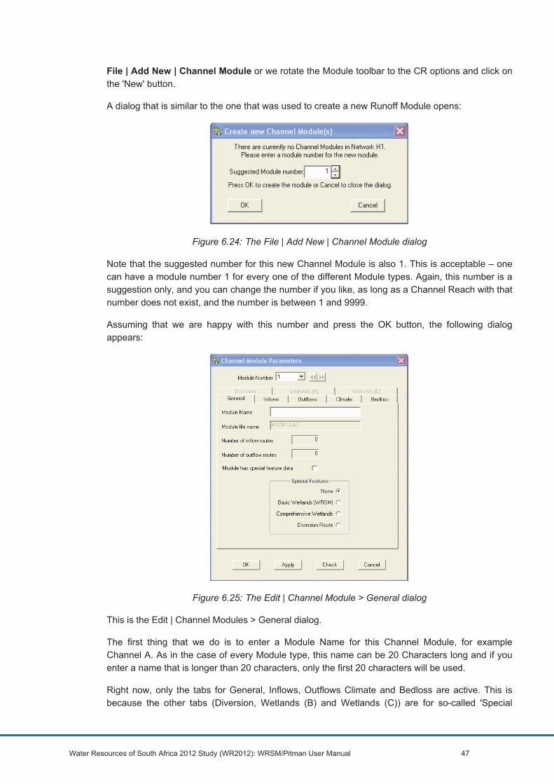
Water Resources of South Africa 2012 Study (WR2012): WRSM/Pitman User Manual 47
File | Add New | Channel Module or we rotate the Module toolbar to the CR options and click on the 'New' button.
A dialog that is similar to the one that was used to create a new Runoff Module opens:
Figure 6.24: The File | Add New | Channel Module dialog
Note that the suggested number for this new Channel Module is also 1. This is acceptable – one can have a module number 1 for every one of the different Module types. Again, this number is a suggestion only, and you can change the number if you like, as long as a Channel Reach with that number does not exist, and the number is between 1 and 9999.
Assuming that we are happy with this number and press the OK button, the following dialog appears:
Figure 6.25: The Edit | Channel Module > General dialog
This is the Edit | Channel Modules > General dialog.
The first thing that we do is to enter a Module Name for this Channel Module, for example Channel A. As in the case of every Module type, this name can be 20 Characters long and if you enter a name that is longer than 20 characters, only the first 20 characters will be used.
Right now, only the tabs for General, Inflows, Outflows Climate and Bedloss are active. This is because the other tabs (Diversion, Wetlands (B) and Wetlands (C)) are for so-called 'Special

Water Resources of South Africa 2012 Study (WR2012): WRSM/Pitman User Manual 48
Features.' As can be seen, when a new Channel Reach Module is created it does not have any special features.
The field File Name contains the name of the file that will be created when the module is saved: The Network name (H1) followed by the abbreviation for this module type (CR) followed by the module number (1) followed by .DAT. The file will be saved in the input directory that we set when we started the new network.
Right now, this Channel Reach has no Inflow routes, and no Outflow routes, and also has no Special Features nor special feature data.
After entering the name of the Channel Module, we press the OK button. The same dialog as Error! Reference source not found. 6.24 will be shown again, ready to create another new channel reach. We do not want one, right now, and so we press the 'Cancel' button.
Now that we have two modules we can continue by adding a few routes.
6.1.11 Adding a Route
To add a Route to our network H1, we select the Menu option
File | Add New | Route or we can rotate the Module toolbar to the RT options and click on the 'New Route' button.
A dialog as follows will open:
Figure 6.26: The File | Add New | Route dialog
By default, the next number for the route is suggested as the Route Number for this route. Again, this is a suggestion only, and you can change the route number to any number between 1 and 9999 (inclusive) for the route to be created, as long as a route of that number does not exist in the network at the moment. In this way you can redefine a route that you deleted before.
By default, the route will run from a Zero Source Module to a Zero Sink Module. The concept of a Zero Source and Zero Sink Modules is described in the section 2.2 of Chapter 2 in this manual.
By clicking on the arrow next to the drop down list box for the “From module”, all modules that are currently in the network are displayed, and you can select one of those. In a similar way, the “To module” for the route is set.
There are all sorts of checks to see whether a route is valid. If you try to add an invalid route (e.g. one that starts and ends in the same module) the route will be rejected. Attempting a circular argument, e.g. by routing the outflows from the Channel Reach back into the Runoff Module may appear to work at first, but will be rejected when a connectivity check is made just before the simulation runs.

Water Resources of South Africa 2012 Study (WR2012): WRSM/Pitman User Manual 49
Let us therefore add a Route from Runoff Module 1 to Channel Reach A:
Figure 6.27: The File | Add New | Route dialog, filled out
When we press the OK button, the following dialog will automatically be displayed:
Figure 6.28: The Edit | Runoff Module | Outflow dialog
This is the Edit | Runoff Modules > Outflow dialog. The route creation routine has recognised that the route that we have just created was an outflow route to a Runoff Module and would now like to know what proportion of the outflow from the Runoff Module should be routed along that new route.
Since there is only one route leaving the Runoff module right now, we must put the Percentage Flow in the dialog to 100%. When we add another outflow route to the Runoff Module, the same dialog will be called up to allow us to control the routing of the outflows. Note that the total percentage outflow must add up to 100% at all times. If this is not the case, an error message will alert you to this.
After we press the OK button in this dialog, the dialog will close, and the dialog as shown in Error! Reference source not found. will once again appear, ready to add the next route.
We now add one outflow route to the Channel Reach Module. This route will go from the Channel Reach to the final Zero Sink Module. The final sink Module is the last Module in a network. All water that runs out of Runoff Module (Runoff 1) into the Channel Reach (Channel Reach A) leaves the network into this Zero Sink Module.

Water Resources of South Africa 2012 Study (WR2012): WRSM/Pitman User Manual 50
Figure 6.29: The File | Add New | Route dialog for the Channel Module outflow route
When we create the route the following dialog will automatically be loaded:
Figure 6.30: The Edit | Route > Defined Flows dialog
This is the Edit | Routes > Defined Flows dialog for route 2. The route creation routine recognised that route number 2 from the Channel Reach to a Zero Sink Module could possibly be a defined route.
A defined route is a route that carries historical flows – flows that we know the value of. Defined flows are historical flows that are used to push (or pull) the flows in the network. As such, defined flows are not the same as observed flows – observed flows are the flows that are used to check the validity of our simulation. This is done at Gauging Stations, about which there will be more later in this document.
In the case where we did have historical data, for example pumping records from a pump that was situated on the banks of the channel, we would insert the file name with those flows into the field marked as Flows File before closing the dialog.
If the route that we had just created was a supply route to an Irrigation Module, the name of this Irrigation Module would have been placed in the field after “Irrigation Module”. This is information only and a reminder that you should not put historical flows in the field that is provided for that purpose – Irrigation blocks are demand centres in their own right, and will try to draw the water that they need by themselves.
In the event that the route that we had just defined routed water from a Reservoir Module, then we could define the monthly abstractions by means of the “Defined Monthly abstractions”. Since

Water Resources of South Africa 2012 Study (WR2012): WRSM/Pitman User Manual 51
the source module for this route is a Channel Reach, however, this option is not available. For this reason, this field is greyed out.
In this case there are no historical (defined) flows to route down this Route – we want this route to carry the final outflows from the Channel reach.
We therefore simply close the dialog again by pressing the OK button.
The same dialog as Error! Reference source not found. now appears again, ready to add more routes, but we close it by pressing the Cancel button.
Should we now attempt to run the simulation (by pressing the running tap button on the toolbar, or choosing the menu point Run | Simulation) we get the message:
Figure 6.31: The Illegal Primary Outflow route dialog
This means that the program has detected an error in the Channel Module number 1, which we called Channel A.
We may have defined an outflow route to this channel Reach, but this route was not defined as the primary outflow route. Even though there is only one outflow route to the Channel Module, it would have been precocious (and possibly wrong) to assume that this route was the primary outflow route.
To fix this, we edit the Channel Module Outflows.
6.1.12 Editing a Channel Module, Outflow Routes
In order to set edit the properties of the Outflow routes of a Channel Reach, we select the menu point Edit | Channel Modules or rotate the Modules toolbar until the Channel Reach (CR) options are uppermost and push the Edit button.
When we have selected the Module with the Module Number 1 and clicked on the Outflows Tab, the following dialog will appear:

Water Resources of South Africa 2012 Study (WR2012): WRSM/Pitman User Manual 52
Figure 6.32: The Edit | Channel Module | Outflows dialog
Currently, our Module 1 has only one outflow route, Route 2. From the listing, we see that route 2 has a Defined code of 'N' from the table of Defined codes, we see that N means that the flows in route 2 are Not defined – they will be calculated.
A primary outflow route is the route that carries the final outflows from the channel reach module. A primary outflow route cannot be a defined route, it cannot be an irrigation abstraction route and it cannot be a Wetlands local outflow route (about which more will be said later). Route 2 has none of these constraints and therefore Route 2 can be used as the primary outflow route.
We select the primary outflow route by opening the drop-down list box next to Primary outflow Route and select Route 2.
By pressing the OK button, the data is stored and the dialog closed.
When we run the simulation now, we get the message:
Figure 6.33: The Simulation Successful dialog
However, at this stage, we do not know how successful the simulation was – we have nothing against which to compare the simulated results. For this reason, we add a Gauging station.

Water Resources of South Africa 2012 Study (WR2012): WRSM/Pitman User Manual 53
6.1.13 Adding a Gauging Station
To add a Gauging Station to the Network, we select the menu point File | Add New | Gauging Station or we rotate the Modules toolbar until the GS options are visible and we press the 'Add New Gauging Station(s)' button.
This action will produce the following dialog:
Figure 6.34: The File | Add New | Gauging Station dialog
A Gauging Station is always situated on an existing Route. Since there are two routes in our Network at this stage, the drop-down list box in this dialog will contain only 2 possibilities on where to place the gauging station: either on route 1 (From Runoff Module 1 to Channel Reach 1) or on Route 2 (From Channel Reach 1 to a Zero Sink Module (ZM0)).
Where you place the gauging station would depend on whether you decide that the gauging station that you have lies above or below the Channel Module. In this case, it was decided that the gauging station lies downstream of the Channel Reach A, on route 2, because that is where the flows in the file “MRA2M50.OBS” stem from.
When one selects this route and presses OK, the following dialog will appear:
Figure 6.35: The Edit | Gauging Station | General dialog
This is the Edit | Gauging Stations > General dialog. In this dialog we can add (or change) the Station name.

Water Resources of South Africa 2012 Study (WR2012): WRSM/Pitman User Manual 54
The Station name would probably be the name of the weir at which the measurements were taken but can be any name that you like. Again the Station name can have a length of up to 20 characters and if you enter a name longer than 20 characters, only the first 20 characters will be saved. The station name will be used in the plots of observed vs. simulated flows, and it would therefore be a good idea to choose the station name well.
The field labelled “File name” is used to specify the name of the file that contains the time series of the observed flows. The flows file can be entered manually, or selected by means of a standard Windows Open File dialog by pressing the seek (...) button next to the input field. In the example that we are working on, the observed flows for the Gauging Station number 1 (GS1) is the file “MRA2M50.OBS”.
The file “MRA2M50.OBS” has the standard flows file format as described in Section 2.3.4 “Flow and .ANS files” in Chapter 2 of this manual.
WRSM/PITMAN can also use SpatSim monthly flows files as observed flows files. Users that have access to the SpatSim database can produce SpatSim text flows and use those as input to the program. SpatSim files are identified by their four header records, for example:
Data: Pitman Sub Dam Sp 1 Downstream Outflow Fixed Interval, Data only: 1 Months: Intervals: Volume: MCM: Start month is October (10) 1920 0.373 0.503 7.670 2.866 0.702 3.734 10.461 4.172 0.990 0.691 0.476 0.352 1921 0.299 4.261 5.895 3.345 1.262 0.499 0.780 1.080 1.326 1.061 0.898 1.458 ...
Note that the “SpatSim.txt” format is different from the standard WRSM format.
The data in the SpatSim file is read with the format '(1X,I4,1X,12(F9.0,1A))', while standard WRSM files are read with the format '(4X,I4,1X,12(F7.0,1A))'
It should be clear that a “SpatSim.txt” file with the header records removed will not be the same as a WRSM/Pitman format file, and removing the header records is therefore not recommended.
The read-only fields “Gauging Station number” and “Associated with route” are there as reminders only that will become especially useful when you start to work with larger networks with many Gauging Stations.
When you press the OK button, the data is saved to memory (though not to disk) and we have a very basic network that can be simulated and calibrated.
6.1.14 Saving the Network
As with every other computer program, it is recommended that while you are working with WRSM/Pitman you should save your data, and save it often.
In WRSM/Pitman one saves the entire network, and not the individual modules, even though the Network and the modules are saved to individual files and you may be asked whether it is allowed to overwrite these files. Saving the Network will automatically save the everything that needs to be saved.
To save the network, you either click on the 'Save Network' button or you select the menu point File | Save | Network.

Water Resources of South Africa 2012 Study (WR2012): WRSM/Pitman User Manual 55
In the event where a file of the same name and path already exists, a dialog will appear as follows:
Figure 6.36: The Output File Check dialog
Pressing the “Quit” button will abort the saving routine.
To change the name of the file to save, one first changes the name in the field and then presses the “Change” button. When the Change button is pressed, a new check will be made to make sure that the new file name that was entered does not exist. Pressing the “Overwrite” button will overwrite the file, and “Overwrite All” will overwrite all files for the entire operation.
“Overwrite All” is valid for the entire Saving operation. If you have made extensive changes to your Network, you may find that it becomes tiresome to press Overwrite every time for every file that was changed while the program saves the data. Pressing Overwrite All once will allow the program to overwrite all module files for the entire saving operation.
Once the saving operation is completed, “Overwrite All” will be reset. If you save the network again, you will once again have the option to Quit, Change, Overwrite or Overwrite All the files.
6.1.15 Exporting a Network to a different folder
Should you wish to export an entire network to a different Folder it is recommended that you change the input and output Folders of your network by means of the dialog Edit | Network > Global.
Figure 6.37: The Edit | Network > Global dialog

Water Resources of South Africa 2012 Study (WR2012): WRSM/Pitman User Manual 56
If you change your Input and (and possibly) Output folders in this dialog, the entire Network will be saved to the new Input Folder, the next time that you choose the File | Save | Network menu point.
Note that time series files (Rainfiles, Observed flows files, defined flows files, etc.) that are used in the network module files will not be exported with these files. Time series files are not copied to avoid the unnecessary duplication of the data. The full path names of Rainfiles and other data files is stored in the Module data files that need the data, and therefore it is possible to store the data in a central directory that can be shared.
Should you wish to distribute a network together with its data files, the data files will have to be copied manually.
6.1.16 Running a Simulation.
To run a simulation, you can either select the menu point Run | Simulation or clicking on the 'running tap' button in the toolbar.
Two operations are carried out before the simulation is run;
a) the data in each of the modules in the Network is checked and b) the connectivity of the modules in the Network is checked.
If there are data errors in the modules, or there are connectivity errors in the network, error messages will show you where those errors are and the simulation will halt.
Data errors can usually be solved by editing the module for which an error was reported and changing the value of the parameter that was indicated or changing the name of the file that was specified.
Connectivity errors are errors where modules have not been connected to downstream modules, or where (such as in the case of Runoff Modules) the distribution of the result flows is not 100% of all flows. In such cases, flows would either be created or destroyed.
In the early stages of a simulation, the simulation may also stop as a result of a sequence error. A sequence error is generated when a particular module expects inflows from an upstream module but that upstream module has not yet been solved.
Sequence errors can only be solved by rearranging the order in which the modules are solved (in the Network dialog).
During the run-up to a simulation, the module and connectivity checks are made silently. This means that no report dialog is generated if a module appears to be correct.
At any time before a simulation is run, the data can be checked by running a separate module check and a separate connectivity check. These tests can be run by choosing the menu points Run | Module Check and Run | Connectivity Check. Note that both these tests are verbose in their singular form and will therefore require quite a lot of interaction.
In most of the Edit dialogs for the different modules in the program, there is a Check button. Pressing this button will run a check on the module data.
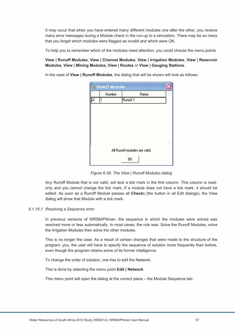
Water Resources of South Africa 2012 Study (WR2012): WRSM/Pitman User Manual 57
It may occur that when you have entered many different modules one after the other, you receive many error messages during a Module check in the run-up to a simulation. There may be so many that you forget which modules were flagged as invalid and which were OK.
To help you to remember which of the modules need attention, you could choose the menu points
View | Runoff Modules, View | Channel Modules, View | Irrigation Modules, View | Reservoir Modules, View | Mining Modules, View | Routes or View | Gauging Stations.
In the case of View | Runoff Modules, the dialog that will be shown will look as follows:
Figure 6.38: The View | Runoff Modules dialog
Any Runoff Module that is not valid, will lack a tick mark in the first column. This column is read-only and you cannot change the tick mark. If a module does not have a tick mark, it should be edited. As soon as a Runoff Module passes all Checks (the button in all Edit dialogs), the View dialog will show that Module with a tick mark.
6.1.16.1 Resolving a Sequence error
In previous versions of WRSM/Pitman, the sequence in which the modules were solved was resolved more or less automatically. In most cases, the rule was: Solve the Runoff Modules, solve the Irrigation Modules then solve the other modules.
This is no longer the case. As a result of certain changes that were made to the structure of the program, you, the user will have to specify the sequence of solution more frequently than before, even though the program retains some of its former intelligence.
To change the order of solution, one has to edit the Network.
This is done by selecting the menu point Edit | Network
This menu point will open the dialog at the correct place – the Module Sequence tab:

Water Resources of South Africa 2012 Study (WR2012): WRSM/Pitman User Manual 58
Figure 6.39: The Edit | Network > Module Sequence dialog
Here you could rearrange the order of solution of the only two modules that we currently have in our Network – RU1 (Runoff Module 1) and CR1 (Channel Module A).
When we click on the CR1 “Module” and then on the “Up” button, the Module CR1 will be moved up one space in the list. If we do this in the current model, this will not have a noticeable effect when the simulation is run since there is no chance of ambiguity, but this will not always be the case.
By means of the tick marks in the column marked “Solve”, it is possible to exclude a module from the simulation process. Note that if you exclude a module from being solved, all downstream modules must also remain unsolved. This is because the downstream modules will expect inflow from the upstream modules. If we were to specify that only RU1 should not be solved, CR1 will detect a sequence error when the simulation is run. The simulation would run if we specified that RU1 should be solved but CR1 should not be solved.
6.1.16.2 Creating a Summary file
Some find it helpful to check the flows in the different routes by means of the summary file. A summary shows the flows in different routes underneath one another, one year per line. You have a free choice as to which Route flows and which Reservoir storages should be written to the file. There is also no limit to the number of summary elements that can be used.
The choice of Routes and Reservoirs and the sequence in which they must appear in the summary file is made in the dialog Edit | Network > Summary this dialog looks as follows:

Water Resources of South Africa 2012 Study (WR2012): WRSM/Pitman User Manual 59
Figure 6.40: The Edit | Network > Summary Dialog
The Routes which can be chosen are in the drop down menu labelled Routes and the Reservoirs in the drop down menu Reservoirs. By selecting one Route or one Reservoir and pressing the Add button, the Route or Reservoir is put in the Summary Elements list. If you want a blank line to separate different blocks of flows, you could add one (or more) by pressing the Blank Line button. After the elements are in the list, the individual elements can be moved up or down in the list by clicking on it to select it and then pressing the Up or Down arrows. To delete an element, click on it to select it and press the Delete button.
When the Summary Elements list contains one or more elements, a summary file will be created automatically when the simulation runs. This file will have a name of the form “H1RUN.SUM” where H1 is the name of the network. Once this file is produced, every subsequent simulation run will ask whether to overwrite this file or not, an output file check just as in the case of the simulation error file.
6.1.17 Actions following a successful simulation
When the simulation ran successfully, the toolbar automatically changes to look as follows
Figure 6.41: The Program Toolbar after a successful Simulation
Two more buttons are now active – one with a Sigma and the one that appears to be a Graph.
Clicking on the button with the sigma is the same as choosing the menu option View | Statistics and clicking on the graph button is the same as choosing the menu point Plot | Plot.
If the simulation reported that there were simulation errors and that you should view the simulations error file, choose the menu option View | Simulation Errors to see what it was that went wrong, and where.

Water Resources of South Africa 2012 Study (WR2012): WRSM/Pitman User Manual 60
6.1.18 Viewing the Statistics
Flow statistics can be viewed for any route in the network, but the statistics for the routes on which there are gauging stations will be the most informative. To view the statistics of a route, either click on the Sigma button or choose the menu point View | Statistics. Either of these operations will result in the following dialog:
Figure 6.42: The View | Statistics dialog
Note that all the fields will be blank, since the program cannot know for which route we would want to view the statistics. We therefore first select the Route Number for which we want to see the statistics. If we choose a route that has a Gauging Station, the number of the gauging station will be shown as read-only information.
By default, the “Statistics Year Start” and “Year End” will be set to the entire simulation period once the route is selected, unless there is a gauging station, where the years are set to cover the period of record. This can be changed to view the statistics of any period with the entire simulation period.
Once the period is set, pressing the “Calculate” button will show the statistics for the simulated flows. If there is a gauging station on the selected route, the statistics for the flows that were observed in this period will be shown under the header 'Observed'.
If the route has an associated gauging station, the program will show hints on how to improve the calibration of the model, but only if the Pitman methodology option has been selected.
In order to implement these hints, there is a further button marked “Edit Runoff”. Pressing this button will call up the Calibration dialog of the Edit Runoff dialog (See Error! Reference source not found.). If the program can determine which Runoff module is unambiguously the only one that will influence the flows in a particular Route, then this Runoff Module is automatically chosen. If not, no Runoff Module is chosen and you will have to choose the module (or modules) to be to be edited yourself.

Water Resources of South Africa 2012 Study (WR2012): WRSM/Pitman User Manual 61
Note that when you are using the Sami on Hughes Groundwater Model in a Runoff Module, it may be necessary to adjust the parameters in the Groundwater dialog of the Edit Runoff dialog in addition to the parameters in the Calibration dialog.
Once the parameters have been adjusted, the Edit Runoff dialog must be closed by pressing the OK button. This will take you back to the dialog above. To see the effects of the changes that you made to the parameters in the Runoff Module, you will have to “Close” this dialog, run the simulation again and after that calculate the statistics anew.
Once you are satisfied with your calibration, you can save the parameters and flows the flows in the route during the simulation to a file by pressing the “Save” button. This will create a file which can be viewed (and optionally printed) by means of the menu point View | Any File. The file name will be shown on the screen when it is created, but it will have the form H1 (for the Network code) followed by RT (for Route) followed by the route number and “.OUT” . The file will be created in the output directory that you specified for the Network.
Note that pressing the Save button will only save the statistics and will not save any of the parameters that you have changed in the Runoff Module to the Runoff Module data file. If you have changed any of the parameters, though, and you attempt to exit the program without having saved them, the program will alert you to this and ask whether you wish to save these parameters.
The statistical parameters are discussed briefly below:
• MAR
If the flow volumes in each year of an n-year record are designated x1, x2, x3,…,xj ,xn;
1 n then MAR = ------ xi n i=1
Due to its computational simplicity, MAR is a commonly used measure of central tendency. However, the median is sometimes to be preferred, especially for extremely skewed distributions.
• Mean (log)
Let yi = log xi then
1 n then Mean (log) = ------ xi n i=1
• Standard Deviation
n Standard Deviation = (xi – MAR)2 / (n – 1) i=1
Standard deviation is the basic measure of variability

Water Resources of South Africa 2012 Study (WR2012): WRSM/Pitman User Manual 62
• Log Standard Deviation
Let yi = log xi then
n LogStandard Deviation = (yi – Standard Deviation)2 / (n – 1) i=1
Logarithmic transformation of streamflow data will usually result in a near normal distribution, i.e. one of minimum skewness. The logarithmic standard deviation has the advantage of being dimensionless and not unduly affected by flood flows.
• Index of seasonal variability (Is)
The index of seasonal variability indicates by means of a simple coefficient the extent of month-by-month fluctuation. It is analogous to the range, taken over a single (season) and therefore represents the storage capacity, as percentage MAR, required to balance the seasonal variations of flow in the river.
The formula is as follows:
Let Qm = mean monthly flow (as %MAR) for each month m, 12 values, then Index = max(sum(Qm-m*100/12)) (for m=1,12) – min(sum(Qm-m*100/12)) (for m=1,12)
6.1.19 Plotting Graphs
The time series of the flows in any route and the storages in any reservoir in the network can be viewed (and printed) from within WRSM/Pitman. In most cases, the graphs of routes on which there are gauging stations will be the most informative, but in some cases much information can also be gleaned from a the simulated values.
A new system for viewing graphs has been implemented making it easy to zoom in or out, pan across or up and down, change to log scale, etc. The manual for using the new graph features has been added as Appendix A
To view the graphs of a route, either click on the Graph button in the toolbar, or choose the menu point Plot | Plot. Either of these operations will result in the following dialog:
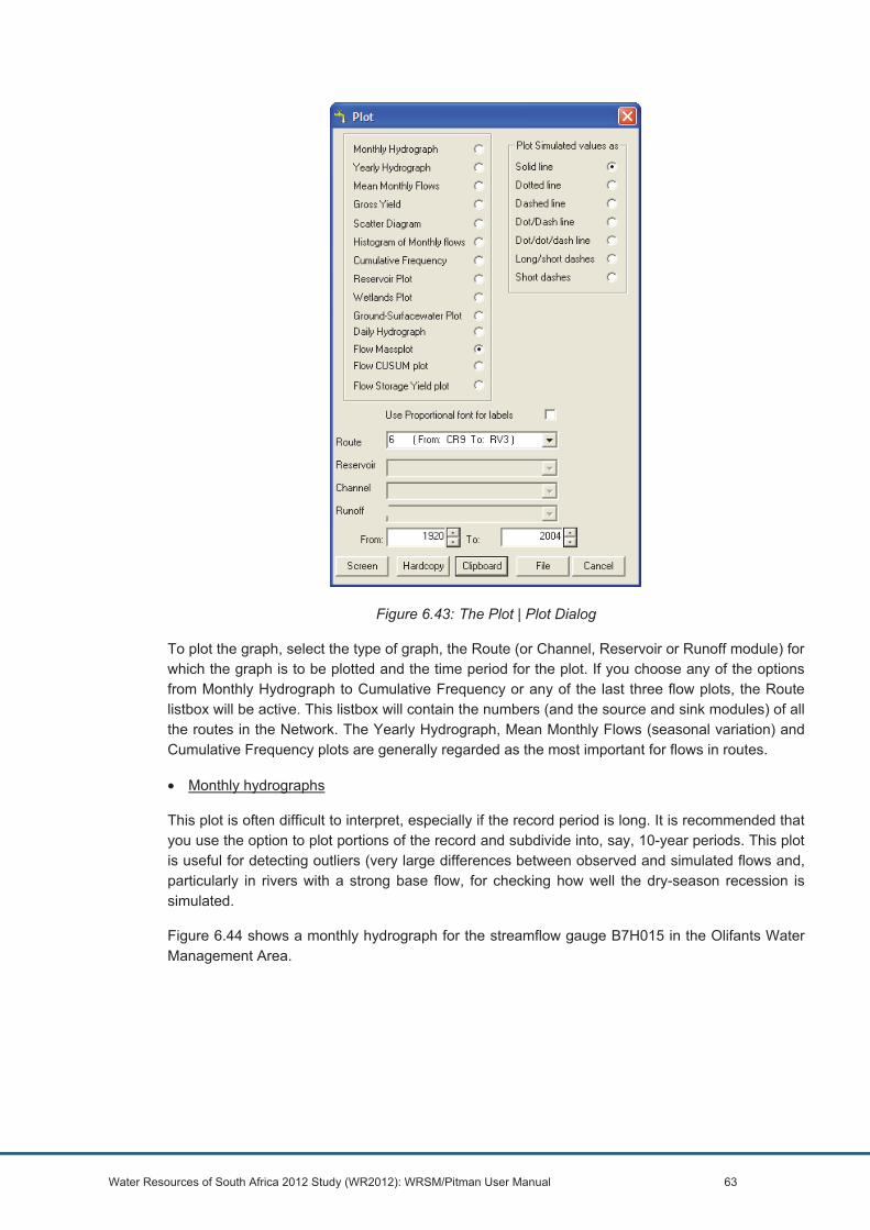
Water Resources of South Africa 2012 Study (WR2012): WRSM/Pitman User Manual 63
Figure 6.43: The Plot | Plot Dialog
To plot the graph, select the type of graph, the Route (or Channel, Reservoir or Runoff module) for which the graph is to be plotted and the time period for the plot. If you choose any of the options from Monthly Hydrograph to Cumulative Frequency or any of the last three flow plots, the Route listbox will be active. This listbox will contain the numbers (and the source and sink modules) of all the routes in the Network. The Yearly Hydrograph, Mean Monthly Flows (seasonal variation) and Cumulative Frequency plots are generally regarded as the most important for flows in routes.
• Monthly hydrographs
This plot is often difficult to interpret, especially if the record period is long. It is recommended that you use the option to plot portions of the record and subdivide into, say, 10-year periods. This plot is useful for detecting outliers (very large differences between observed and simulated flows and, particularly in rivers with a strong base flow, for checking how well the dry-season recession is simulated.
Figure 6.44 shows a monthly hydrograph for the streamflow gauge B7H015 in the Olifants Water Management Area.
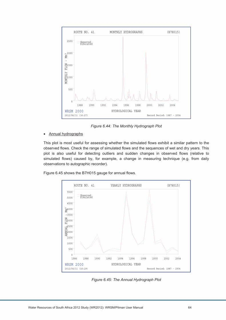
Water Resources of South Africa 2012 Study (WR2012): WRSM/Pitman User Manual 64
Figure 6.44: The Monthly Hydrograph Plot
• Annual hydrographs
This plot is most useful for assessing whether the simulated flows exhibit a similar pattern to the observed flows. Check the range of simulated flows and the sequences of wet and dry years. This plot is also useful for detecting outliers and sudden changes in observed flows (relative to simulated flows) caused by, for example, a change in measuring technique (e.g. from daily observations to autographic recorder).
Figure 6.45 shows the B7H015 gauge for annual flows.
Figure 6.45: The Annual Hydrograph Plot
MONTHLY HYDROGRAPHS
HYDROLOGICAL YEAR
MONTHLY FLOW - Mm³
1988 1990 1992 1994 1996 1998 2000 2002 20040
500
1000
1500
2000
2500 Observed Simulated
ROUTE NO. 41 (B7H015)
WRSM 20002012/06/11 (16:27) Record Period: 1987 - 2004
YEARLY HYDROGRAPHS
HYDROLOGICAL YEAR
ANNUAL FLOW - Mm³
1986 1988 1990 1992 1994 1996 1998 2000 2002 20040
500
1000
1500
2000
2500
3000
3500
4000
4500
5000
5500Observed Simulated
ROUTE NO. 41 (B7H015)
WRSM 20002012/06/11 (16:29) Record Period: 1987 - 2004
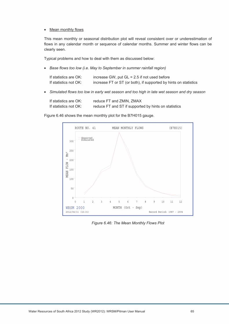
Water Resources of South Africa 2012 Study (WR2012): WRSM/Pitman User Manual 65
• Mean monthly flows
This mean monthly or seasonal distribution plot will reveal consistent over or underestimation of flows in any calendar month or sequence of calendar months. Summer and winter flows can be clearly seen.
Typical problems and how to deal with them as discussed below:
• Base flows too low (i.e. May to September in summer rainfall region)
If statistics are OK: increase GW, put GL = 2.5 if not used before If statistics not OK: increase FT or ST (or both), if supported by hints on statistics
• Simulated flows too low in early wet season and too high in late wet season and dry season
If statistics are OK: reduce FT and ZMIN, ZMAX If statistics not OK: reduce FT and ST if supported by hints on statistics
Figure 6.46 shows the mean monthly plot for the B7H015 gauge.
Figure 6.46: The Mean Monthly Flows Plot
MEAN MONTHLY FLOWS
MONTH (Oct - Sep)
MEAN FLOW - Mm³
0 1 2 3 4 5 6 7 8 9 10 11 120
50
100
150
200
250
300Observed Simulated
ROUTE NO. 41 (B7H015)
WRSM 20002012/06/11 (16:31) Record Period: 1987 - 2004

Water Resources of South Africa 2012 Study (WR2012): WRSM/Pitman User Manual 66
• Gross Yield curves
The firm yields of various dam sizes are computed for the observed and simulated records and plotted as yield curves. Since the yields will be based only on the driest (worst) portion of the record they should be used with caution when calibrating. However, if the simulated yields are high and the hints on the statistics suggest that FT (perennial river) be reduced or that ZMIN (intermittent river) be increased, then following these hints will also being the yield curves closer together.
Figure 6.47 shows the gross yield plot for the B7H015 gauge.
Figure 6.47: The Gross Yield Plot
• Scatter diagram
This plot is most useful for showing up outliers. The coefficient of efficiency "E" (see top left corner of plot) is indicative of the goodness-of-fit and a value of 0.8 or higher can be considered good. However, the presence of just one outlier can reduce E considerably.
Figure 6.48 shows a scatter plot for the B7H015 gauge.
GROSS YIELD
STORAGE CAPACITY - Mm³
GROSS
YIELD - Mm³ p.a.
0 500 1000 1500 2000 2500 3000 3500 40000
100
200
300
400
500
600
700
800
900
1000
1100
Observed Simulated
ROUTE NO. 41 (B7H015)
WRSM 20002012/06/11 (16:49) Record Period: 1987 - 2004

Water Resources of South Africa 2012 Study (WR2012): WRSM/Pitman User Manual 67
Figure 6.48: The Scatter Diagram
• Histogram
This plot indicates whether or not the model is simulating low flows accurately. It is, however, easier to interpret plot No.7 (cumulative frequency).
Figure 6.49 shows the histogram for the B7H015 gauge.
Figure 6.49: The Monthly Histogram
SCATTER DIAGRAM
OBSERVED FLOW - Mm³
SIMULATED FLOW - Mm³
0 500 1000 1500 2000 25000
500
1000
1500
2000
2500
øø
øøøø
øøøøøøøø øøøøøøøøøøø
øøøøø øøøøøøøøø
ø øø
øøøøøøøøøøøøøøøøøøøøøøøøøøøøøøøø
øøøøøøøøøøøøøøøøøøøøøøøøø
ø
ø
ø
øø
øøøøøø
ø øø
øø
ø øøøøø
øøø
øøøøøøøøøø
ø ø
øøøøøøøøøøø
ø
ø
ø
ø
øøøøøøø
øøøøøøøøøø ø
øø
øøøøøøøøøøøøøøøøøøøøøøøøøø
øø
øøøøøøøøøøøøøøøøø
E = 0.96
ROUTE NO. 41
WRSM 20002012/06/11 (16:47) Record Period: 1987 - 2004
MONTHLY HISTOGRAM
MONTHLY FLOW - Mm³
FREQUENCY - % total
0 20 40 60 80 100 120 140 160 180 2000
5
10
15
20
25 Observed Simulated
ROUTE NO. 41 (B7H015)
WRSM 20002012/06/11 (16:50) Record Period: 1987 - 2004

Water Resources of South Africa 2012 Study (WR2012): WRSM/Pitman User Manual 68
• Cumulative frequency
The cumulative frequency (or duration) curve shows the percentage time that various flows are equalled or exceeded. If the tail of the simulated duration curve is above the observed curve (to the right on the graph), the following action can be taken:
If statistics are OK: reduce GW If statistics not OK: reduce FT if supported by hints on statistics.
Figure 6.50 shows the cumulative frequency for the B7H015 gauge.
Figure 6.50: The Cumulative Frequency Plot
• Reservoir Plot
When you choose 'Reservoir Plot', the Reservoir listbox will be active and Route, Channel and Runoff will be inactive. Both the draft (abstractions from the dam) and storage state plots will be shown one underneath the other.
The user can add an observed storage state percentage curve to the simulated by selecting a datafile of observed percentage storages. This file must cover the same period as the start and end date of the dam (as entered in the reservoir module). The format is the same as that for any input or output abstraction or return flow except that the values are in percentage form (see example below)
2004 90.57 82.09 81.24 94.87 99.98 99.74 99.84 99.75 99.69 99.59 97.84 88.79 2005 74.82 57.21 55.10 68.03 100.69 101.78 101.02 100.33 99.98 99.89 99.81 99.41 2006 95.08 89.15 95.97 101.45 99.77 100.03 97.87 99.78 98.02 95.57 92.80 86.91 2007 74.16 71.13 84.29 99.98 100.17 100.06 99.90 99.86 99.44 98.44 94.38 87.65 2008 77.65 64.55 66.20 83.96 103.37 101.49 100.22 99.96 99.82 99.76 99.75 97.17
The resulting file must be saved as a text file for reading by the model.
The Reservoir Record is obtainable from DWS and must be set up in the right format outside of the WRSM/Pitman model. A program called “Reservoir Record format” to do this exists
CUMULATIVE FREQUENCY
MONTHLY FLOW - Mm³
FREQUENCY - %
total
0 20 40 60 80 100 120 140 160 180 2000
10
20
30
40
50
60
70
80
90
Observed Simulated
ROUTE NO. 41 (B7H015)
WRSM 20002012/06/11 (16:35) Record Period: 1987 - 2004

Water Resources of South Africa 2012 Study (WR2012): WRSM/Pitman User Manual 69
(developed by Mr John Hansford while at Knight Piesold which is now available from Mr Allan Bailey of Royal HaskoningDHV) .
Figure 6.51 shows the reservoir trajectory for Blyderivierspoort Dam.
Figure 6.51: The Reservoir Trajectory Plot
• Wetlands Plot
When you choose Wetlands Plot, the Channel listbox will be active because a Wetland is always associated with a Channel Reach and Route, Reservoir and Runoff will be inactive. Both the draft (abstractions from the wetland) and storage state plots will be shown one underneath the other.
The wetlands plot is exactly the same as a reservoir plot and an example will therefore not be shown.
• Ground-Surfacewater Plot
When you choose 'Ground-Surfacewater Plot', the Runoff listbox will be active and Route, Reservoir and Wetland will be inactive, because the Groundwater-Surface water interaction is always associated with a Runoff module. The net catchment runoff (total of surface and groundwater flow) will be shown in blue. For Hughes there is no interflow or total groundwater outflow, just the baseflow/discharge. This graph is shown in purple. For Sami, the groundwater outflow is the baseflow/discharge plus interflow and is shown in red. As for Hughes, the baseflow/discharge is shown in purple. The interflow is shown in green.
Baseflow/discharge and interflow and other groundwater terms are defined in section 6.1.27.3.
In the Hughes method, interflow is treated as part of the original POW and FT function (unchanged except for the removal of SL as a possible limiting value). There is therefore no distinction in the Hughes method between soil moisture flow and interflow within the unsaturated zone and therefore total groundwater outflow and interflow cannot be shown.
This plot is for a runoff module as a whole and should not be confused with flow in a route. This plot shows the time series available under File | Save for net catchment runoff, groundwater outflow, groundwater baseflow/discharge (Sami method only) and groundwater (Sami method only). The time series for groundwater outflow may contain small negative values which is
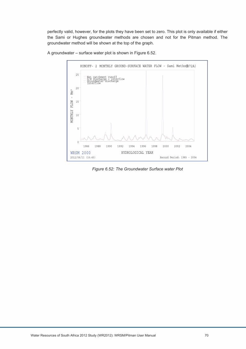
Water Resources of South Africa 2012 Study (WR2012): WRSM/Pitman User Manual 70
perfectly valid, however, for the plots they have been set to zero. This plot is only available if either the Sami or Hughes groundwater methods are chosen and not for the Pitman method. The groundwater method will be shown at the top of the graph.
A groundwater – surface water plot is shown in Figure 6.52.
Figure 6.52: The Groundwater Surface water Plot
MONTHLY GROUND-SURFACE WATER FLOW - Sami Method
HYDROLOGICAL YEAR
MONTHLY FLOW - Mm³
1986 1988 1990 1992 1994 1996 1998 2000 2002 20040
5
10
15
20
25Net catchment runoffG/W discharge + interflowGroundwater dischargeInterflow
RUNOFF- 2 (B72A)
WRSM 20002012/06/11 (16:45) Record Period: 1985 - 2004

Water Resources of South Africa 2012 Study (WR2012): WRSM/Pitman User Manual 71
• Daily Hydrograph – naturalised
If the daily time step is used, it will be possible to plot a daily hydrograph of naturalised streamflow emanating from any runoff module as shown in Figure 6.53 for example. Daily flow is plotted in cubic metres per second over the record period. If the record period is lengthy, it will probably be necessary to plot certain smaller ranges of start and end year to examine what is happening with the flow. .
Figure 6.53: The Daily Hydrograph – naturalised flow
DAILY HYDROGRAPHS
HYDROLOGICAL YEAR
DAILY FLOW - m³/s
1962 1963 1964 1965 1966 1967 1968 1969 1970 1971 1972 1973 19740
20
40
60
80
100
120
140
Naturalised daily runoff
WRSM 20002012/06/11 (16:20) Record Period: 1962 - 1973

Water Resources of South Africa 2012 Study (WR2012): WRSM/Pitman User Manual 72
• Daily Hydrograph – including land use
Once the required daily simulated streamflow has been determined as described in section 10.6 and the daily observed file is available in a folder in the correct format (as shown in 10.6), then a plot of the daily simulated versus the daily observed can be obtained as shown in Figure 6.54 . as above, daily flow is plotted in cubic metres per second over the record period. If the record period is lengthy, it will probably be necessary to plot certain smaller ranges of start and end year to examine what is happening with the flow.
Observed and simulated statistics have been determined in a similar way to the monthly time step and these have been superimposed in a corner of the graph as shown.
Figure 6.54: The Daily Hydrograph including land use

Water Resources of South Africa 2012 Study (WR2012): WRSM/Pitman User Manual 73
• Flow Massplot
The “flow Massplot” should only really be used for naturalised monthly streamflow but can be used for streamflow which includes the effects of land/water use. The cumulative flows are plotted against time as shown in Figure 6.55 below. It is similar to the rainfall massplot but tends to be more sensitive to climatic variations owing to non-linear relationship between rainfall and runoff. A typical curve (as is Figure 6.55) will depict several short periods of steep slope, associated with flood events, interspersed with flatter slopes representing average to dry periods. The overall trend should, however, be linear. A distinct change in slope could represent a problem with the rainfall data and/or patching of missing and/or unreliable values
Figure 6.55: The Streamflow Massplot
STREAMFLOW MASSPLOT
HYDROLOGICAL YEAR
Cumulative Flow - Mm3
1920 1930 1940 1950 1960 1970 1980 1990 20000
200
400
600
800
1000
1200
1400
1600
1800
2000
2200
2400Simulated
ROUTE NO. 6
WRSM 20002012/06/11 (15:05) Record Period: 1920 - 2004

Water Resources of South Africa 2012 Study (WR2012): WRSM/Pitman User Manual 74
• Flow CUSUM Plot
The “streamflow cusum” plot is also intended for naturalised monthly streamflow but can also be plotted for streamflow which includes the effects of land/water use. The mean annual runoff (MAR) is determined and the cumulative summations (“cusum”) are then determined by taking the cumulative streamflow and subtracting an equivalent number of months of MAR. A typical “cusum” plot is given in Figure 6.56 below. The “cusum” plot gives a more sensitive picture of the variation in streamflow than the massplot. In some periods this result will be positive and for other periods it will be negative. Ideally the positives should more or less be balanced out by the negatives. Typically, the plot shows steep positive slopes during periods of high runoff associated with floods, followed by flatter negative slopes during periods of average to below average streamflow. For example, Figure 6.56 shows a period of high runoff in the 1970s, followed by a period of below average runoff lasting until the mid-1990s. The graph will start at zero (one month before the start of the record period) and end at zero. If the curve is mostly in the positive territory, this implies an overall decline in runoff over time and vice versa. A curve that is always either in the positive or negative territory would be extremely unusual and would indicate some error in the catchment rainfall. In such cases one should refer back to the rainfall “cusum” plot to check for any anomalies.
Figure 6.56: The Streamflow CUSUM Plot
STREAMFLOW CUSUM PLOT
HYDROLOGICAL YEAR
Cum. Flow less mean - Mm3
1920 1930 1940 1950 1960 1970 1980 1990 2000
-40
-20
0
20
40
60
80
100
120Simulated
ROUTE NO. 6
WRSM 20002012/06/11 (15:13) Record Period: 1920 - 2004
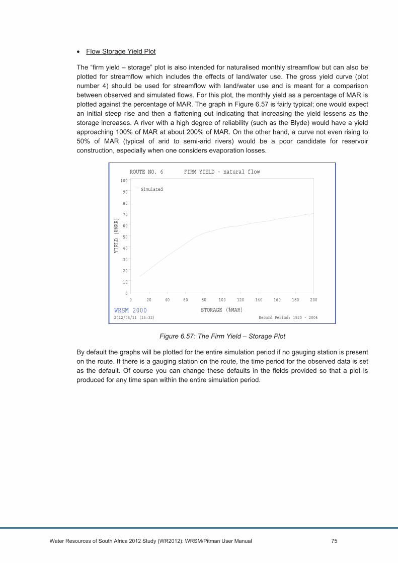
Water Resources of South Africa 2012 Study (WR2012): WRSM/Pitman User Manual 75
• Flow Storage Yield Plot
The “firm yield – storage” plot is also intended for naturalised monthly streamflow but can also be plotted for streamflow which includes the effects of land/water use. The gross yield curve (plot number 4) should be used for streamflow with land/water use and is meant for a comparison between observed and simulated flows. For this plot, the monthly yield as a percentage of MAR is plotted against the percentage of MAR. The graph in Figure 6.57 is fairly typical; one would expect an initial steep rise and then a flattening out indicating that increasing the yield lessens as the storage increases. A river with a high degree of reliability (such as the Blyde) would have a yield approaching 100% of MAR at about 200% of MAR. On the other hand, a curve not even rising to 50% of MAR (typical of arid to semi-arid rivers) would be a poor candidate for reservoir construction, especially when one considers evaporation losses.
Figure 6.57: The Firm Yield – Storage Plot
By default the graphs will be plotted for the entire simulation period if no gauging station is present on the route. If there is a gauging station on the route, the time period for the observed data is set as the default. Of course you can change these defaults in the fields provided so that a plot is produced for any time span within the entire simulation period.
FIRM YIELD - natural flow
STORAGE (%MAR)
YIELD (%MAR)
0 20 40 60 80 100 120 140 160 180 2000
10
20
30
40
50
60
70
80
90
100
Simulated
ROUTE NO. 6
WRSM 20002012/06/11 (15:32) Record Period: 1920 - 2004
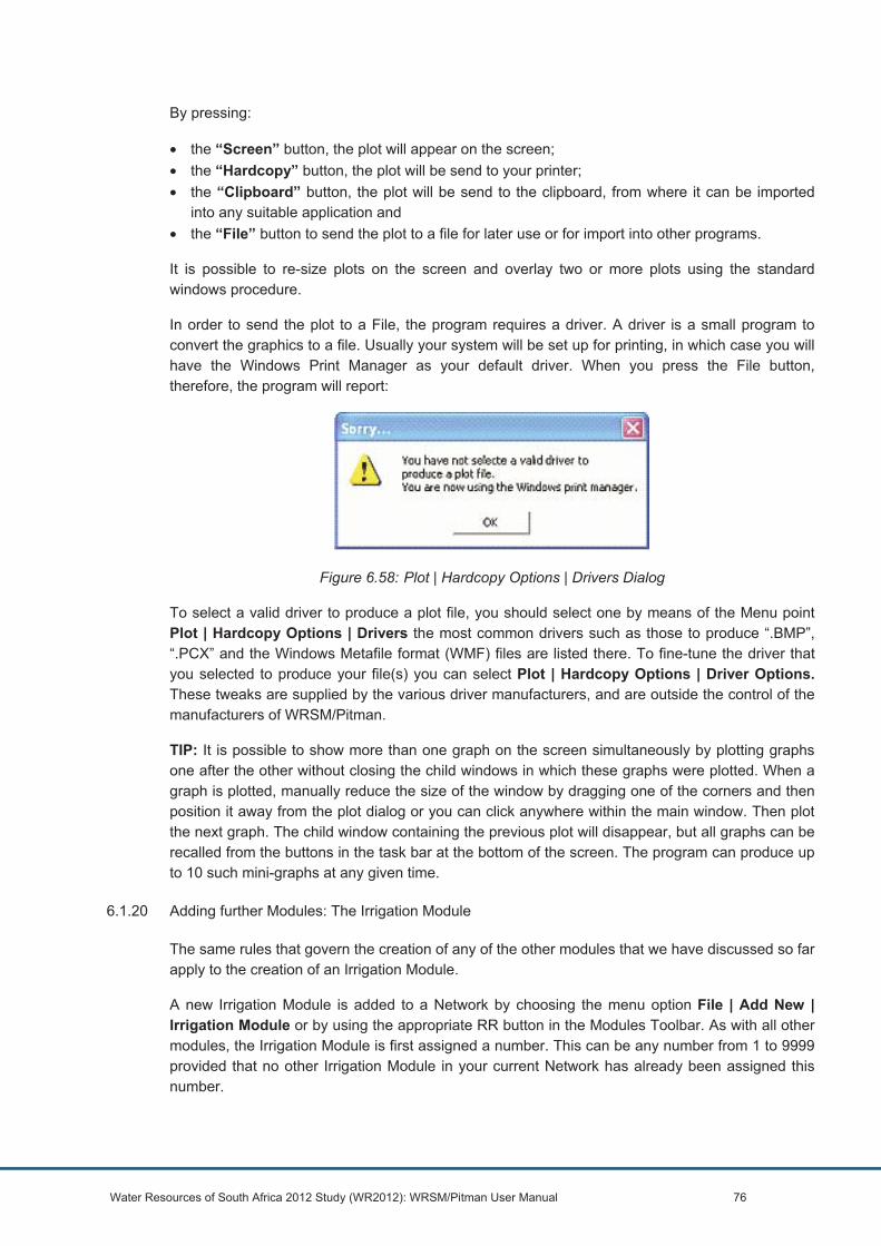
Water Resources of South Africa 2012 Study (WR2012): WRSM/Pitman User Manual 76
By pressing:
• the “Screen” button, the plot will appear on the screen; • the “Hardcopy” button, the plot will be send to your printer; • the “Clipboard” button, the plot will be send to the clipboard, from where it can be imported
into any suitable application and • the “File” button to send the plot to a file for later use or for import into other programs.
It is possible to re-size plots on the screen and overlay two or more plots using the standard windows procedure.
In order to send the plot to a File, the program requires a driver. A driver is a small program to convert the graphics to a file. Usually your system will be set up for printing, in which case you will have the Windows Print Manager as your default driver. When you press the File button, therefore, the program will report:
Figure 6.58: Plot | Hardcopy Options | Drivers Dialog
To select a valid driver to produce a plot file, you should select one by means of the Menu point Plot | Hardcopy Options | Drivers the most common drivers such as those to produce “.BMP”, “.PCX” and the Windows Metafile format (WMF) files are listed there. To fine-tune the driver that you selected to produce your file(s) you can select Plot | Hardcopy Options | Driver Options. These tweaks are supplied by the various driver manufacturers, and are outside the control of the manufacturers of WRSM/Pitman.
TIP: It is possible to show more than one graph on the screen simultaneously by plotting graphs one after the other without closing the child windows in which these graphs were plotted. When a graph is plotted, manually reduce the size of the window by dragging one of the corners and then position it away from the plot dialog or you can click anywhere within the main window. Then plot the next graph. The child window containing the previous plot will disappear, but all graphs can be recalled from the buttons in the task bar at the bottom of the screen. The program can produce up to 10 such mini-graphs at any given time.
6.1.20 Adding further Modules: The Irrigation Module
The same rules that govern the creation of any of the other modules that we have discussed so far apply to the creation of an Irrigation Module.
A new Irrigation Module is added to a Network by choosing the menu option File | Add New | Irrigation Module or by using the appropriate RR button in the Modules Toolbar. As with all other modules, the Irrigation Module is first assigned a number. This can be any number from 1 to 9999 provided that no other Irrigation Module in your current Network has already been assigned this number.

Water Resources of South Africa 2012 Study (WR2012): WRSM/Pitman User Manual 77
Once the Irrigation Module has been assigned its number and you press the OK button, the program will automatically open the Edit | Irrigation Modules > General dialog. This dialog looks as follows in 6.59
6.1.20.1 Editing the Irrigation Module: General Dialog
Figure 6.59: The Edit | Irrigation Module > General dialog
The first thing to do is to enter the Module Name. This can be any name that you choose and although you can enter a name of any length, only the first 20 characters will be saved.
The field Module File Name is read-only and contains the name of the file that will be created when you save the module. In this case it is the network name (H1) followed by the abbreviation for Irrigation Modules (RR) followed by the module number (1) followed by “.DAT”. This file will be saved in the input directory that you specified for your Network.
When an Irrigation Module is created, it does not yet have an Abstraction Route – the route that will carry water to this module – nor will it have a Return Flow Route (the route that carries return flows away from the Irrigation Module). These routes are defined separately once the module is created, just like before, by means of defining new routes File | Add New | Route
You have a choice of four Model Types that can be used to simulate the flows in an Irrigation Block Module, the Original WRSM/Pitman model, the WQT model, the WQT-SAPWAT model or the WQT Type 4 model. Once you have selected the model to use and you press the Apply button, certain of the tabs will be switched off – this is because the four models require different types of input.
The input requirements for the three methods are briefly described as follows:
• Original WRSM2000 – only one set of crop factors, no allowance for canal losses or efficiency, return flow as a proportion of water applied.
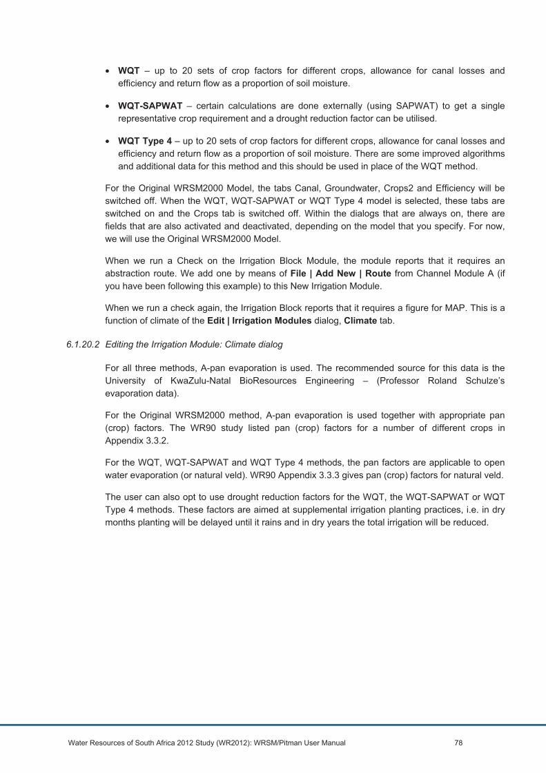
Water Resources of South Africa 2012 Study (WR2012): WRSM/Pitman User Manual 78
• WQT – up to 20 sets of crop factors for different crops, allowance for canal losses and efficiency and return flow as a proportion of soil moisture.
• WQT-SAPWAT – certain calculations are done externally (using SAPWAT) to get a single representative crop requirement and a drought reduction factor can be utilised.
• WQT Type 4 – up to 20 sets of crop factors for different crops, allowance for canal losses and efficiency and return flow as a proportion of soil moisture. There are some improved algorithms and additional data for this method and this should be used in place of the WQT method.
For the Original WRSM2000 Model, the tabs Canal, Groundwater, Crops2 and Efficiency will be switched off. When the WQT, WQT-SAPWAT or WQT Type 4 model is selected, these tabs are switched on and the Crops tab is switched off. Within the dialogs that are always on, there are fields that are also activated and deactivated, depending on the model that you specify. For now, we will use the Original WRSM2000 Model.
When we run a Check on the Irrigation Block Module, the module reports that it requires an abstraction route. We add one by means of File | Add New | Route from Channel Module A (if you have been following this example) to this New Irrigation Module.
When we run a check again, the Irrigation Block reports that it requires a figure for MAP. This is a function of climate of the Edit | Irrigation Modules dialog, Climate tab.
6.1.20.2 Editing the Irrigation Module: Climate dialog
For all three methods, A-pan evaporation is used. The recommended source for this data is the University of KwaZulu-Natal BioResources Engineering – (Professor Roland Schulze’s evaporation data).
For the Original WRSM2000 method, A-pan evaporation is used together with appropriate pan (crop) factors. The WR90 study listed pan (crop) factors for a number of different crops in Appendix 3.3.2.
For the WQT, WQT-SAPWAT and WQT Type 4 methods, the pan factors are applicable to open water evaporation (or natural veld). WR90 Appendix 3.3.3 gives pan (crop) factors for natural veld.
The user can also opt to use drought reduction factors for the WQT, the WQT-SAPWAT or WQT Type 4 methods. These factors are aimed at supplemental irrigation planting practices, i.e. in dry months planting will be delayed until it rains and in dry years the total irrigation will be reduced.
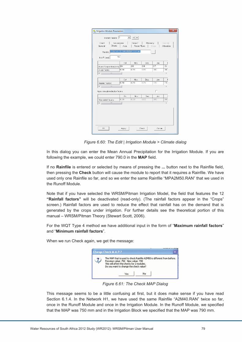
Water Resources of South Africa 2012 Study (WR2012): WRSM/Pitman User Manual 79
Figure 6.60: The Edit | Irrigation Module > Climate dialog
In this dialog you can enter the Mean Annual Precipitation for the Irrigation Module. If you are following the example, we could enter 790.0 in the MAP field.
If no Rainfile is entered or selected by means of pressing the ... button next to the Rainfile field, then pressing the Check button will cause the module to report that it requires a Rainfile. We have used only one Rainfile so far, and so we enter the same Rainfile “MPA2M50.RAN” that we used in the Runoff Module.
Note that if you have selected the WRSM/Pitman Irrigation Model, the field that features the 12 “Rainfall factors” will be deactivated (read-only). (The rainfall factors appear in the “Crops” screen.) Rainfall factors are used to reduce the effect that rainfall has on the demand that is generated by the crops under irrigation. For further details see the theoretical portion of this manual – WRSM/Pitman Theory (Stewart Scott, 2006).
For the WQT Type 4 method we have additional input in the form of “Maximum rainfall factors” and “Minimum rainfall factors”.
When we run Check again, we get the message:
Figure 6.61: The Check MAP Dialog
This message seems to be a little confusing at first, but it does make sense if you have read Section 6.1.4. In the Network H1, we have used the same Rainfile “A2M40.RAN” twice so far, once in the Runoff Module and once in the Irrigation Module. In the Runoff Module, we specified that the MAP was 750 mm and in the Irrigation Block we specified that the MAP was 790 mm.

Water Resources of South Africa 2012 Study (WR2012): WRSM/Pitman User Manual 80
It is perfectly valid to specify a different MAP for the same Rainfile – if you know that the figure is correct. The Rainfile simply specifies the time series of monthly rainfall as percentage of MAP and so although the distribution of the rainfall is the same, it may be that the MAP. on the Irrigation Block is indeed 40 mm higher than it is for the rest of the catchment.
When a Rainfile is used for the first time, the MAP that is used in conjunction with this time series is kept in memory with the data for the Rainfile. This figure is called the Check MAP.
All that this message is saying, therefore, is that a different M.A.P. is used with the same rainfall distribution file, and that the value of 750 mm will be used to check whether the MAP in any module that uses this Rainfile deviates from the 'normal'. If you have many modules that are going to use this Rainfile, and most of them have a Mean Annual Precipitation of 790 mm then you can change the check value to minimise the number of times that the program complains about the difference.
Note that no matter what you answer to this question, it will NOT affect the MAPs in the Modules. As the dialog states, you can only change the MAP against which the check is made.
6.1.20.3 The Irrigation Module Abstraction Route.
When we run a Check on the Irrigation Module, the program will report that the Irrigation Module does not have an Abstraction route. An Abstraction route is a route that brings water to the Irrigation module.
We create a new Route by means of the menu point File | Add New | Route. The new route, Route 3 will run from Channel Module A to Irrigation Block 1, (or CR1 to RR1).
Although it is possible to abstract water directly from a Runoff Module into an Irrigation Block Module, this is not recommended.
An Irrigation block is a Demand Centre. This means that the Irrigation Block will calculate its own specific demands for a specific month and year, depending on the needs of the crops that are grown in the Irrigation Block and the area under irrigation. Once those demands are calculated, the demand is placed into the Abstraction Route. When the simulation runs, the Module that is to supply this demand (in this case the Channel Reach) will determine how much water it can supply to the Irrigation block. If not enough water is available to supply the entire demand of the Irrigation Block, the supplied flow in the Irrigation Abstraction Route will be reduced. In this way, we simulate a run-of-river irrigation scheme. A reservoir supported irrigation scheme is simulated by connecting the Abstraction Route of an Irrigation Block Module to a Reservoir Module.
Note 1: If an irrigation block requires more water than that which is available, the WRSM/Pitman model will run successfully and the deficits will be reported under “simulation errors”.
Note 2: If a system has irrigation blocks and defined abstraction datafiles, then the defined abstractions will be satisfied first and then the irrigation blocks. IF there is insufficient water for the irrigation blocks, the run will fail and an error message will appear on the screen. The user should then review both the irrigation blocks and the abstraction datafiles to reduce the demand. It is also possible that the runoff sub-model may not be providing enough flow.
It should now be clear that is does not make sense to connect the Abstraction Route of an Irrigation Block to the outflow of the Runoff Module. This action would 'force' water through an Irrigation Block Module, and would cause massive over-watering of the crops during the wetter periods, thus drowning them. Not only would this annoy the “simulated” farmers, but since

Water Resources of South Africa 2012 Study (WR2012): WRSM/Pitman User Manual 81
Irrigation Blocks can be simulated without Return Flow Routes, this could cause the model to lose water.
Irrigation Block Modules should therefore only draw water from a Reservoir Module or from a Channel Reach Module.
A further way to control the abstractions that are made by an Irrigation Block is discussed under Channel Reach Module: the Diversion Channel in Section 6.2
When we view the Routes with the menu point View | Routes, we will see the following dialog:
Figure 6.62: The View | Routes dialog
Note that Route 3 has an "I" in the 'Defined' column. That means that the Route is an Irrigation Abstraction Route. An “N” means that the route is not defined, i.e. that flows in it will be calculated by the upstream module.
Either by attempting to Run the simulation or by Editing the Irrigation Block Module and running a Check on it, you will find that an irrigation block needs 12 monthly Evaporation Values.
You can add these values in the Edit | Irrigation Modules > Climate dialog (above) either manually or by copying them from the Runoff Module that we created before.
To Copy and Paste monthly values from one module to another, select the module with the values, click on the label of the row that you wish to copy (i.e. either Evaporation or Pan Factor) and the entire row is selected. Move the mouse to the October value, right click and select 'copy' from the floating menu. Select the module into which you wish to paste the values, click the same label, right click the October value and select Paste. The keyboard functions “Ctrl-C” and “Ctrl-V” can, of course, also be used.
A further press on the Check button reveals that the Irrigation Module has no year / area curve points.
Figure 6.63: The Missing Area Data Dialog in Irrigation Blocks
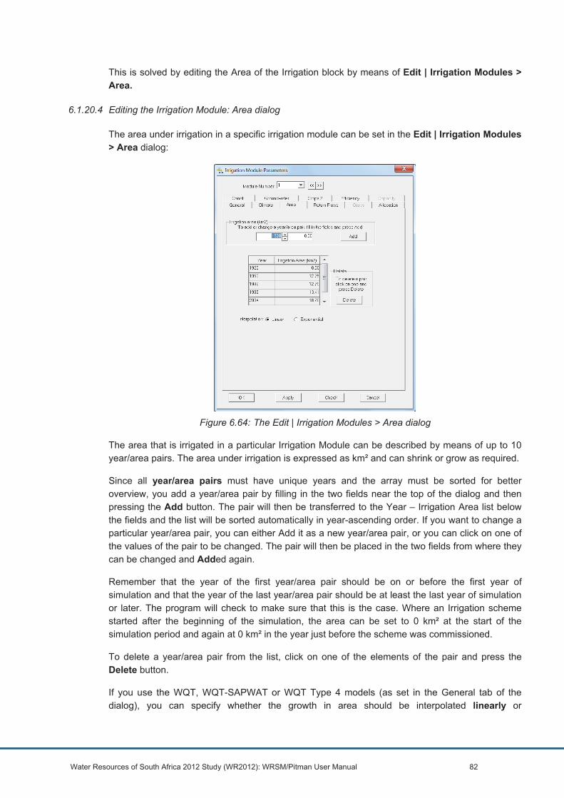
Water Resources of South Africa 2012 Study (WR2012): WRSM/Pitman User Manual 82
This is solved by editing the Area of the Irrigation block by means of Edit | Irrigation Modules > Area.
6.1.20.4 Editing the Irrigation Module: Area dialog
The area under irrigation in a specific irrigation module can be set in the Edit | Irrigation Modules > Area dialog:
Figure 6.64: The Edit | Irrigation Modules > Area dialog
The area that is irrigated in a particular Irrigation Module can be described by means of up to 10 year/area pairs. The area under irrigation is expressed as km² and can shrink or grow as required.
Since all year/area pairs must have unique years and the array must be sorted for better overview, you add a year/area pair by filling in the two fields near the top of the dialog and then pressing the Add button. The pair will then be transferred to the Year – Irrigation Area list below the fields and the list will be sorted automatically in year-ascending order. If you want to change a particular year/area pair, you can either Add it as a new year/area pair, or you can click on one of the values of the pair to be changed. The pair will then be placed in the two fields from where they can be changed and Added again.
Remember that the year of the first year/area pair should be on or before the first year of simulation and that the year of the last year/area pair should be at least the last year of simulation or later. The program will check to make sure that this is the case. Where an Irrigation scheme started after the beginning of the simulation, the area can be set to 0 km² at the start of the simulation period and again at 0 km² in the year just before the scheme was commissioned.
To delete a year/area pair from the list, click on one of the elements of the pair and press the Delete button.
If you use the WQT, WQT-SAPWAT or WQT Type 4 models (as set in the General tab of the dialog), you can specify whether the growth in area should be interpolated linearly or
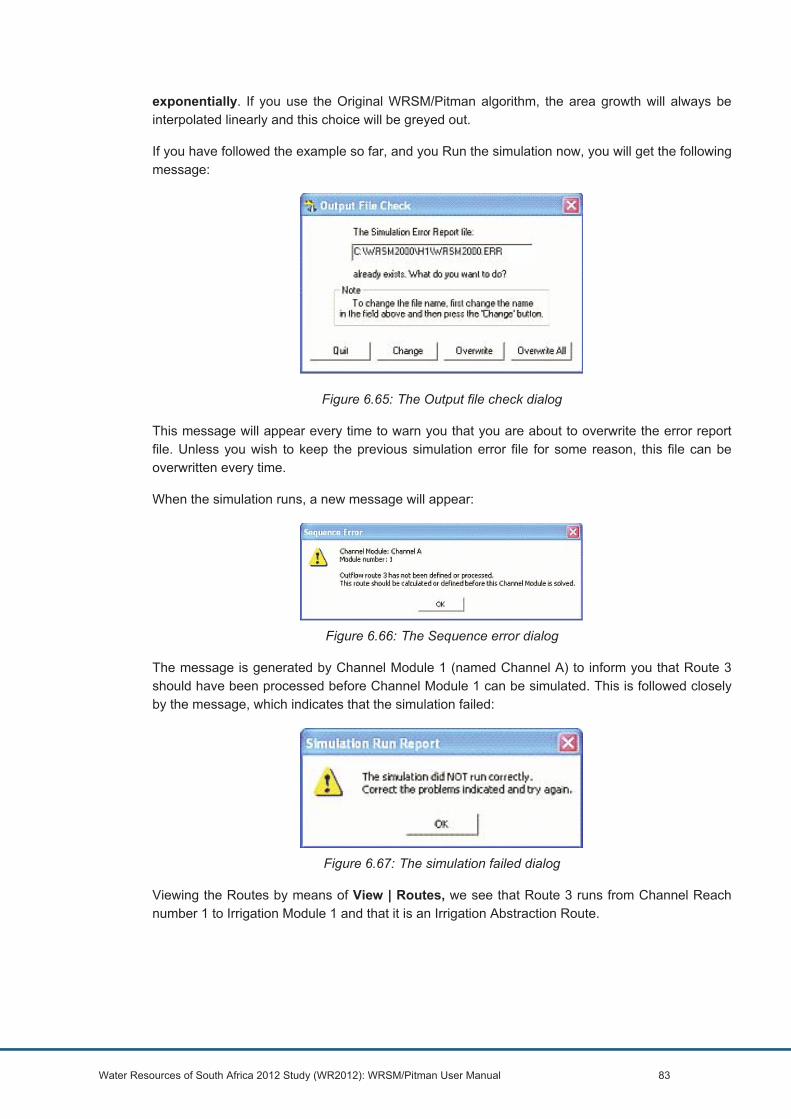
Water Resources of South Africa 2012 Study (WR2012): WRSM/Pitman User Manual 83
exponentially. If you use the Original WRSM/Pitman algorithm, the area growth will always be interpolated linearly and this choice will be greyed out.
If you have followed the example so far, and you Run the simulation now, you will get the following message:
Figure 6.65: The Output file check dialog
This message will appear every time to warn you that you are about to overwrite the error report file. Unless you wish to keep the previous simulation error file for some reason, this file can be overwritten every time.
When the simulation runs, a new message will appear:
Figure 6.66: The Sequence error dialog
The message is generated by Channel Module 1 (named Channel A) to inform you that Route 3 should have been processed before Channel Module 1 can be simulated. This is followed closely by the message, which indicates that the simulation failed:
Figure 6.67: The simulation failed dialog
Viewing the Routes by means of View | Routes, we see that Route 3 runs from Channel Reach number 1 to Irrigation Module 1 and that it is an Irrigation Abstraction Route.

Water Resources of South Africa 2012 Study (WR2012): WRSM/Pitman User Manual 84
Figure 6.68: The View | Routes dialog
From this we suspect that the order (or sequence) of solution in the Network is at fault. The demanded abstraction flows that are placed in Route 3 are placed there by calculating the Demands of Irrigation Block Module 1.
Checking the solution sequence in the dialog Edit | Network, we see the following:
Figure 6.69: The Edit | Network > Module sequence dialog
Indeed, it is specified that the demands from the Irrigation Block Module are calculated AFTER the flows in Channel Reach Module 1 are calculated. To solve this problem, we either click on the Module RR1 and move it Up to above CR1 OR we click on Module CR1 and move it Down below RR1.
It should be appreciated that the flows within Route 3 may be calculated twice, and that a route, in effect, contains two 'streams' – the 'demand' stream and the 'supply' stream.
During the simulation of an Irrigation Module, the flows that are demanded by the crops in the irrigation module are placed in the 'demand' stream of the Irrigation Abstraction Route (Route 3). After it has done that, the Irrigation Module assumes that these demands will be supplied somehow. It therefore calculates its own losses, the storage to groundwater and its own return flows based on this assumption.

Water Resources of South Africa 2012 Study (WR2012): WRSM/Pitman User Manual 85
Once that is done, following the sequence of solution, the simulation for the Channel Reach Module is done. The simulation of a Channel Module involves the adding all the inflows to the module and then subtracting the proposed outflows to see whether enough water is available. In this step, the demands from the Irrigation Module are taken as part of the proposed outflows.
If there is enough water to supply these demands, the value from the 'demand' stream of Route 3 is copied to the 'supply' stream, and no further action is necessary.
If there is not enough water to supply the demands, the flow in the 'supply' stream of Route 3 is reduced. The amount of water that actually reaches the Irrigation module is therefore less than what the module demanded. The Channel Module 'knows' that it is supplying less water than it was asked for, and therefore sends a message to the Irrigation module to signal that the Irrigation Module should re-simulate itself. The Irrigation Module does this, and recalculates all the losses, storages and return flows based on the supply that it received.
For a more detailed description of deficit handling, see Chapter 9.
As before, a Return Flow Route for an Irrigation Module can be added to the Network by means of the menu point File | Add New | Route and specifying the Irrigation Module as the Upstream module to this new Route.
Since Return Flows from an Irrigation Module will be recalculated in the event of a deficit, it should be clear why the model does not allow the routing of the return flows from an Irrigation Module into the same module that supplies the Irrigation Block. Such a construct could lead to a potentially never-ending circular argument. Return Flow Routes may only be connected to Zero Sink Modules or to modules that are downstream of the module that supplies an Irrigation Block.
For guidance on how to enter information for the remaining Irrigation dialogs (Crops, Allocation, Crops2, Canal, Groundwater, Efficiency, Return Flows and Capacity), refer to section 6.1.22 .
6.1.21 Adding further Modules: The Reservoir Module
Up to 9999 Reservoir Modules may be added to a given network, given that you have enough memory in your computer. Adding a Reservoir Module to a network follows the same principle as adding a Runoff Module or a Channel Reach Module: by choosing the menu option File | Add New | Reservoir or selecting the new Reservoir button from the RV buttons in the Modules Toolbar.
Just as in the case of the Runoff Module and the Channel Reach Module, creating a new reservoir module starts with determining the number of the module. Again, this number can be any number from 1 to 9999 and the module number must be unique for all the Reservoirs in the Network.
Once the question of the number is settled, and the OK button is pressed, the program will automatically open the dialog:

Water Resources of South Africa 2012 Study (WR2012): WRSM/Pitman User Manual 86
Figure 6.70: The Edit | Reservoir Modules > General dialog
This is the dialog that can also be reached by means of the menu point
Edit | Reservoir Modules > General.
In this dialog we enter the name of the reservoir in the field after Module Name. Again, the maximum length of the name is limited to 20 characters.
The field next to the label Module file name is the name of the file that will be created when the Reservoir Module is saved. The name consists of the name of the Network (H1) followed by the abbreviation for Reservoir (RV) followed by the number that we gave this Reservoir (1), followed by “DAT”. The file will be created in the input directory of the Network.
When it is created, the Reservoir Module does not have any inflow Routes or outflow Routes. These are created by means of the menu point File | Add New | Route.
The default initial storage is 50% of the total storage of the reservoir. When there is a tick mark next to the label Use default initial storage, the reservoir will therefore be at 50% when the simulation starts – provided, of course, that the reservoir had already been built at the beginning of the simulation.
If there is a tick mark next to Use default initial storage, the field Starting Storage (million m³) will be inactive. As soon as you remove the tick mark, the field for Starting Storage will be activated and you can enter the starting storage that you want.
Should you close the dialog and attempt to run the simulation, you will get the message:
Figure 6.71: The missing inflow routes dialog for Reservoirs

Water Resources of South Africa 2012 Study (WR2012): WRSM/Pitman User Manual 87
We therefore add two routes – an inflow route from Runoff Module 1 to Reservoir 1 and an outflow route that connects Reservoir 1 to Channel Reach 1.
As soon as we add Route from the Runoff Module RU1 to the Reservoir Module RV1, we get the following dialog:
Figure 6.72: The Edit | Runoff Modules > Outflow dialog
This is the Edit | Runoff Modules > Outflow dialog again. If we leave things as they are, 0% of the runoff that is generated by the Runoff Module will be routed towards the new reservoir, which is clearly not what we want. On the other hand, we must make sure that the total percentage of outflow is exactly 100% or we will either create or destroy flows. Let us therefore set the percentage outflow along Route 1 to the Channel Module at 43% and the percentage outflow to the Reservoir along route 4 at 57%.
After that we can close the dialog by pressing the OK button.
When we create the Reservoir Spillage route, Route 5, the following dialog pops up:

Water Resources of South Africa 2012 Study (WR2012): WRSM/Pitman User Manual 88
Figure 6.73: The Edit | Route | Defined Flows dialog
This is the Edit | Routes > Defined Flows dialog. We have the opportunity here to enter a defined Flows file or a set of 12 Defined monthly abstractions. The Defined monthly abstractions dialog was always inactive when we created routes before because this option is only available for Routes that lead from Reservoirs.
We did not see this dialog when we created the route from the Runoff Module to the Reservoir Module, because such routes cannot have defined flows. A Runoff Module is a Source Centre and placing an observed flow on a route that emerges from a Runoff Module would either 'boost' or 'throttle' the flows, which would cause the model to either gain or lose flows.
We do not enter any flows in the Defined monthly abstractions fields – or in the Flows File field, for that matter – because we would like the reservoir to spill via this route. We close the dialog without making any changes by pressing the OK button.
Should we attempt to run the model, we will get the message:
Figure 6.74: The Illegal spillage route dialog for Reservoirs
This is the same type of error that we got when we did not specify the Primary Outflow Route to the Channel Module (See Figure 6.29 in Section 6.1.8.) Although there is only one outflow route to the Reservoir, the model cannot 'know' that you really want this route to be your Spillage route.

Water Resources of South Africa 2012 Study (WR2012): WRSM/Pitman User Manual 89
To solve this problem, we edit Reservoir Module 1 by means of the menu point Edit | Reservoir Modules, selecting Reservoir Module Number 1 and clicking on the Outflow tab. The dialog that this produces looks as follows:
Figure 6.75: The Edit | Reservoir Modules > Outflow dialog
As we already know, the list of routes in this Module shows that there is only one outflow route to this Reservoir: Route 5. This route has an “N” is the Defined column, which means that the flows in the route will be calculated. This is therefore a suitable route to use as a Spillage route.
If the Route had been a defined route, there would have been an “F” in the Defined column, and a file name in the File Name column. If the route was an Abstraction Route for an Irrigation module, there would have been an “I” in the Defined column and if we had defined 12 monthly abstractions there would have been an M in the Defined column.
All routes that have defined codes other than “N” should be considered unsuitable as Spillage Route, even though it is allowed to use a defined flow route for historical reasons: In the past when creating a route was still a major operation, some users insisted on creating as few routes as possible and treating historical releases as spills.
Note that although the model will handle this scenario correctly, this arrangement may be the cause of some confusion:
During the simulation, the Reservoir Module will first accumulate all the inflows and service all the defined outflows before it services the calculated demands (such as those from Irrigation Modules). After allowance is made for evaporation, etc., the model checks whether the final storage is greater than the Full Supply Volume. If the final storage is greater than FSV, the reservoir spills via the spillage route.
If we put defined flows in the spillage route, the Reservoir will spill when the defined flows dictate that it should do so, regardless of whether the Reservoir is full or not. On the other hand, if the simulation is not quite calibrated yet, the model will add the spillages that it calculated to the defined flows that it already placed in the spillage route. With the defined spillage scenario it may therefore be a problem to distinguish 'real' from 'defined' spills.

Water Resources of South Africa 2012 Study (WR2012): WRSM/Pitman User Manual 90
In our example, no “Spillage route” has been defined yet. To define the spillage route, we click on the arrow next to the drop down list box next to the label “Spillage route” and select route number 5. We can the close the dialog by pressing the OK button.
Attempting to run the program again will result is the message:
Figure 6.76: The missing MAP dialog for Reservoirs
Since the storage in a Reservoir is influenced by the amount of rain that falls over the Reservoir, it is clear that both a Rainfile and an MAP must be supplied for every Reservoir. We do this in the Edit | Reservoir Modules > Climate dialog.
This dialog is similar to the dialog that is produced for every other module in WRSM/Pitman:
Figure 6.77: The Edit | Reservoir Modules > Climate dialog
When you have selected the module to edit in the field next to Module Number, the Rainfile (as described in Section 6.1.4 and the MAP for the reservoir can be entered. Note that different modules may share a Rainfile, even though the MAP may be different.
In order to calculate the evaporation from the reservoir, you should also add the 12 monthly Symons Pan evaporation values in the space provided, as well as the Pan Factors. For pan factors, WR90 Appendix 3.3.1 can be used (lake evaporations).
To Copy and Paste monthly values from one module to another:
a) Select the Module with the values, click on the label of the row that you wish to copy (i.e. either Evaporation or Pan Factor) and the entire row is selected.
b) Move the mouse to the October value, right click and select 'copy' from the floating menu.

Water Resources of South Africa 2012 Study (WR2012): WRSM/Pitman User Manual 91
c) Select the Module into which you wish to paste the values, click the same label, right click the October value and select Paste. The keyboard functions Ctrl-C and Ctrl-V can, of course, also be used.
Closing the dialog and attempting to Run the simulation again will now produce the message:
Figure 6.78: The Missing Year/Area/Volume Data Dialog for Reservoirs
This means that we have not yet completed the physical characteristics of our Reservoir – we still have to add at least two year – area – volume triplet parameters.
We do this in the Edit | Reservoir Modules > Storage dialog:
Figure 6.79: The Edit Reservoir > Storage dialog
When we have selected the Reservoir that we wish to edit in the field after Module Number, we can add the year/area/volume data. As in the case of the year/area data pairs in the Irrigation block that we discussed in the previous section, the triplets that we add here must be in chronological sequence. For this reason, we have a mask in which we enter the three values before we press the Add button to transfer the data to the list below the mask.
Note that the first triplet must have a year-value that is either in (or before) the first year of simulation, and the last year must be in (or after) the last year of the simulation. If the entire simulation period is not covered, the program will not be able to calculate the values for area and volume for the years that lie outside your data. The data will, of course be checked for validity before the simulation runs.
In the event that the reservoir was built after the start of the simulation, you can start with a 1900-0-0 triplet and another 19xx-0-0 just before the dam is commissioned. As the Reservoir silts up, so the area and volume can be reduced, and a heightening of the dam wall can be simulated by
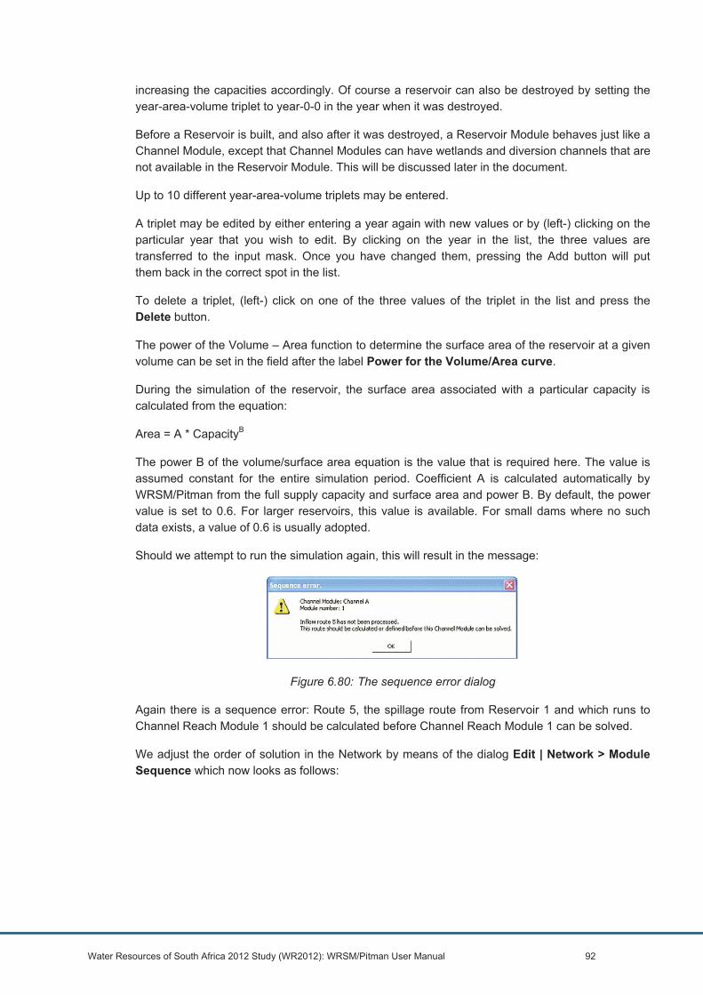
Water Resources of South Africa 2012 Study (WR2012): WRSM/Pitman User Manual 92
increasing the capacities accordingly. Of course a reservoir can also be destroyed by setting the year-area-volume triplet to year-0-0 in the year when it was destroyed.
Before a Reservoir is built, and also after it was destroyed, a Reservoir Module behaves just like a Channel Module, except that Channel Modules can have wetlands and diversion channels that are not available in the Reservoir Module. This will be discussed later in the document.
Up to 10 different year-area-volume triplets may be entered.
A triplet may be edited by either entering a year again with new values or by (left-) clicking on the particular year that you wish to edit. By clicking on the year in the list, the three values are transferred to the input mask. Once you have changed them, pressing the Add button will put them back in the correct spot in the list.
To delete a triplet, (left-) click on one of the three values of the triplet in the list and press the Delete button.
The power of the Volume – Area function to determine the surface area of the reservoir at a given volume can be set in the field after the label Power for the Volume/Area curve.
During the simulation of the reservoir, the surface area associated with a particular capacity is calculated from the equation:
Area = A * CapacityB
The power B of the volume/surface area equation is the value that is required here. The value is assumed constant for the entire simulation period. Coefficient A is calculated automatically by WRSM/Pitman from the full supply capacity and surface area and power B. By default, the power value is set to 0.6. For larger reservoirs, this value is available. For small dams where no such data exists, a value of 0.6 is usually adopted.
Should we attempt to run the simulation again, this will result in the message:
Figure 6.80: The sequence error dialog
Again there is a sequence error: Route 5, the spillage route from Reservoir 1 and which runs to Channel Reach Module 1 should be calculated before Channel Reach Module 1 can be solved.
We adjust the order of solution in the Network by means of the dialog Edit | Network > Module Sequence which now looks as follows:
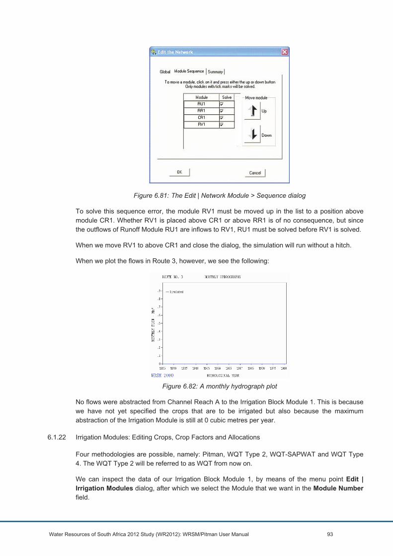
Water Resources of South Africa 2012 Study (WR2012): WRSM/Pitman User Manual 93
Figure 6.81: The Edit | Network Module > Sequence dialog
To solve this sequence error, the module RV1 must be moved up in the list to a position above module CR1. Whether RV1 is placed above CR1 or above RR1 is of no consequence, but since the outflows of Runoff Module RU1 are inflows to RV1, RU1 must be solved before RV1 is solved.
When we move RV1 to above CR1 and close the dialog, the simulation will run without a hitch.
When we plot the flows in Route 3, however, we see the following:
Figure 6.82: A monthly hydrograph plot
No flows were abstracted from Channel Reach A to the Irrigation Block Module 1. This is because we have not yet specified the crops that are to be irrigated but also because the maximum abstraction of the Irrigation Module is still at 0 cubic metres per year.
6.1.22 Irrigation Modules: Editing Crops, Crop Factors and Allocations
Four methodologies are possible, namely: Pitman, WQT Type 2, WQT-SAPWAT and WQT Type 4. The WQT Type 2 will be referred to as WQT from now on.
We can inspect the data of our Irrigation Block Module 1, by means of the menu point Edit | Irrigation Modules dialog, after which we select the Module that we want in the Module Number field.

Water Resources of South Africa 2012 Study (WR2012): WRSM/Pitman User Manual 94
If you specified that you want to use the Pitman irrigation model in this Irrigation Module in the Edit | Irrigation Modules > General dialog, only the General, Climate, Area, Return Flow, Crops and Allocation tabs will be activated.
If you specified that you wanted to use the WQT, WQT-SAPWAT or WQT Type 4 Irrigation models, then the tabs Canal, Groundwater, Crops2 and Efficiency will be active, but the tab Crops will be deactivated. For WQT Type 4 there is also a Capacity tab.
You may swap between the two irrigation models by selecting the Edit | Irrigation Modules > General dialog and selecting the Irrigation model that you want to use by clicking on the radio button next to the model that you want. Once you have done that, it is necessary to press the Apply button, so that all data that you may have changed in the model that you had selected previously can be saved and the tabs in the main dialog switched on or off as the case may be.
For a description of the dialog for the WQT, WQT-SAPWAT or WQT Type 4 Irrigation Model, see section 6.1.22.2.
6.1.22.1 Editing Crops, Crop Factors and Allocations for the Pitman Irrigation Model
If we press the tab Crops in the Edit | Irrigation Modules menu point, we see the following dialog:
Figure 6.83: The Edit | Irrigation Modules > Crops dialog
In this dialog, we can edit the proportion of the total area under irrigation that is irrigated in a particular month, the “P-Index”. The effective rainfall factors are set for every month in the line “Eff. Rain factor”. Clearly the P-Index can never be greater than 1.00 or less than 0.00. Since the areas that are irrigated in any given month is currently 0.00 throughout, the Irrigation Module in the example did not produce any demands.
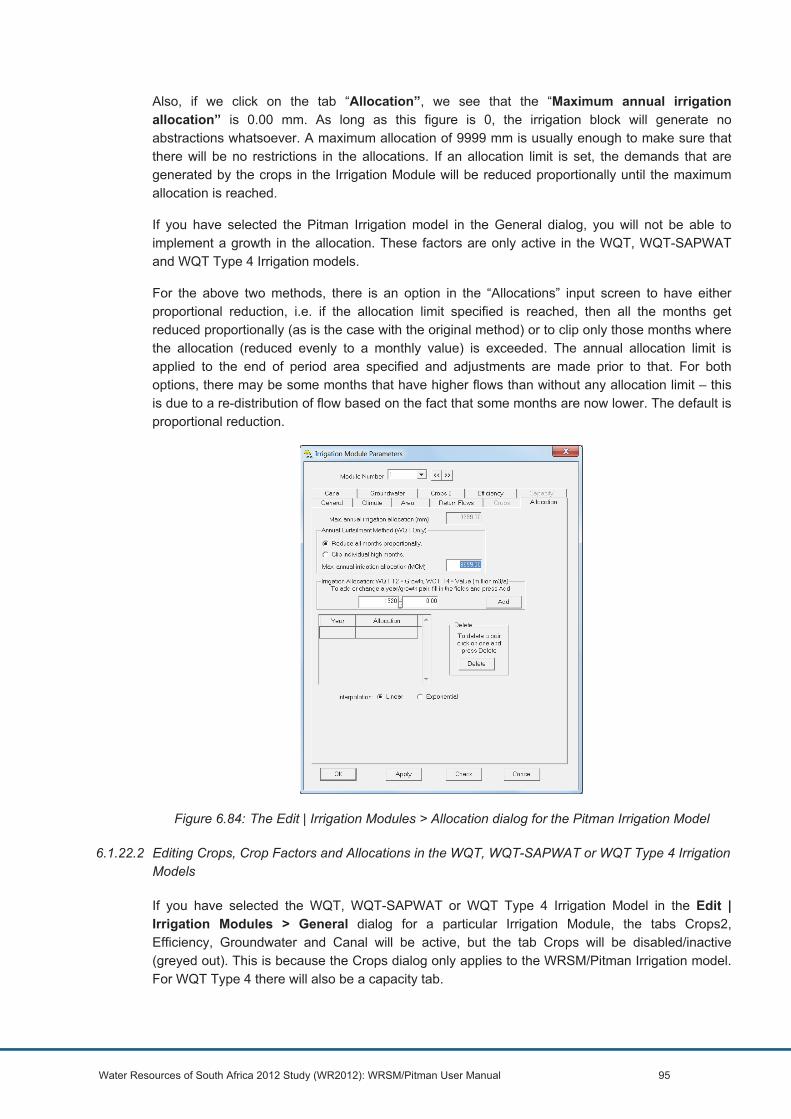
Water Resources of South Africa 2012 Study (WR2012): WRSM/Pitman User Manual 95
Also, if we click on the tab “Allocation”, we see that the “Maximum annual irrigation allocation” is 0.00 mm. As long as this figure is 0, the irrigation block will generate no abstractions whatsoever. A maximum allocation of 9999 mm is usually enough to make sure that there will be no restrictions in the allocations. If an allocation limit is set, the demands that are generated by the crops in the Irrigation Module will be reduced proportionally until the maximum allocation is reached.
If you have selected the Pitman Irrigation model in the General dialog, you will not be able to implement a growth in the allocation. These factors are only active in the WQT, WQT-SAPWAT and WQT Type 4 Irrigation models.
For the above two methods, there is an option in the “Allocations” input screen to have either proportional reduction, i.e. if the allocation limit specified is reached, then all the months get reduced proportionally (as is the case with the original method) or to clip only those months where the allocation (reduced evenly to a monthly value) is exceeded. The annual allocation limit is applied to the end of period area specified and adjustments are made prior to that. For both options, there may be some months that have higher flows than without any allocation limit – this is due to a re-distribution of flow based on the fact that some months are now lower. The default is proportional reduction.
Figure 6.84: The Edit | Irrigation Modules > Allocation dialog for the Pitman Irrigation Model
6.1.22.2 Editing Crops, Crop Factors and Allocations in the WQT, WQT-SAPWAT or WQT Type 4 Irrigation Models
If you have selected the WQT, WQT-SAPWAT or WQT Type 4 Irrigation Model in the Edit | Irrigation Modules > General dialog for a particular Irrigation Module, the tabs Crops2, Efficiency, Groundwater and Canal will be active, but the tab Crops will be disabled/inactive (greyed out). This is because the Crops dialog only applies to the WRSM/Pitman Irrigation model. For WQT Type 4 there will also be a capacity tab.
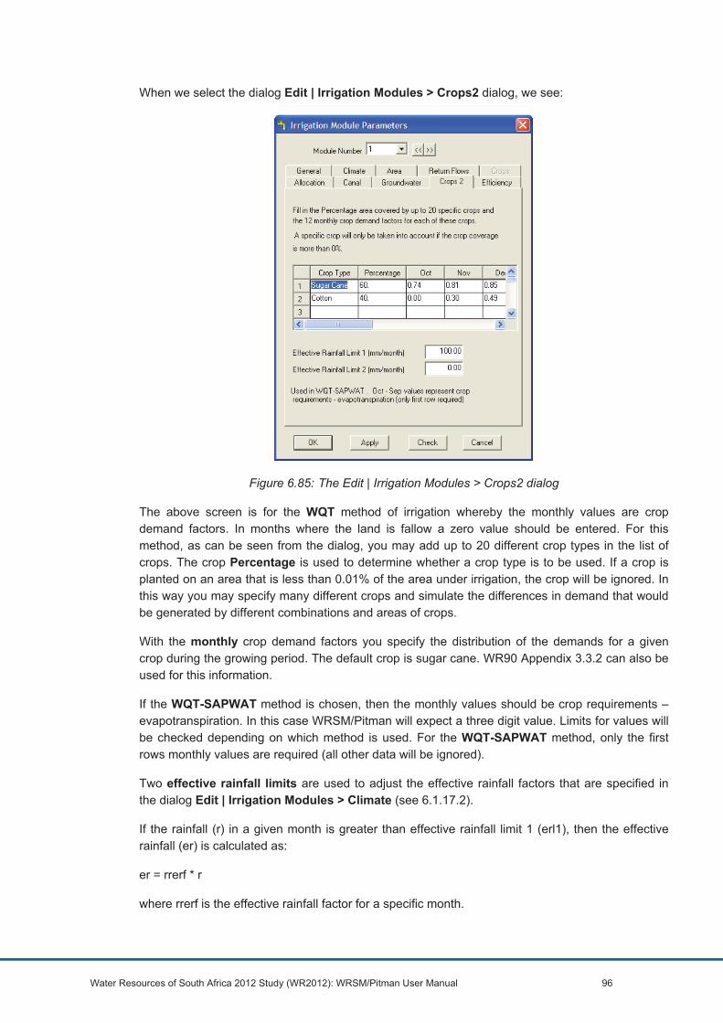
Water Resources of South Africa 2012 Study (WR2012): WRSM/Pitman User Manual 96
When we select the dialog Edit | Irrigation Modules > Crops2 dialog, we see:
Figure 6.85: The Edit | Irrigation Modules > Crops2 dialog
The above screen is for the WQT method of irrigation whereby the monthly values are crop demand factors. In months where the land is fallow a zero value should be entered. For this method, as can be seen from the dialog, you may add up to 20 different crop types in the list of crops. The crop Percentage is used to determine whether a crop type is to be used. If a crop is planted on an area that is less than 0.01% of the area under irrigation, the crop will be ignored. In this way you may specify many different crops and simulate the differences in demand that would be generated by different combinations and areas of crops.
With the monthly crop demand factors you specify the distribution of the demands for a given crop during the growing period. The default crop is sugar cane. WR90 Appendix 3.3.2 can also be used for this information.
If the WQT-SAPWAT method is chosen, then the monthly values should be crop requirements – evapotranspiration. In this case WRSM/Pitman will expect a three digit value. Limits for values will be checked depending on which method is used. For the WQT-SAPWAT method, only the first rows monthly values are required (all other data will be ignored).
Two effective rainfall limits are used to adjust the effective rainfall factors that are specified in the dialog Edit | Irrigation Modules > Climate (see 6.1.17.2).
If the rainfall (r) in a given month is greater than effective rainfall limit 1 (erl1), then the effective rainfall (er) is calculated as:
er = rrerf * r
where rrerf is the effective rainfall factor for a specific month.

Water Resources of South Africa 2012 Study (WR2012): WRSM/Pitman User Manual 97
If the rainfall (r) in a given month is less than effective rainfall limit 1 (erl1) but greater than effective rainfall limit 2 (erl2), then the effective rainfall factor (erf) is calculated as:
erf = rrerf + (rrerfM – rrerf) * (erl1 – r) / (erl1 – erl2) where rrerfM is the maximum effective rainfall factor for the month
from which the effective rainfall (er) is then calculated as
er = erf * r
If the rainfall is less than rainfall limit 2 (erl2) then the effective rainfall is set to the rainfall in that month, i.e.
er = r
If the rainfall is less than the limit 2, all of the rainfall is considered effective. If it is above the upper limit 1, then the user defined effective rainfall factor is applied. If the monthly rainfall is between these two limits, then the effective rainfall factor is interpolated linearly between 1 and the nominal effective rainfall factor. In other words, default limits of 100 (limit 1) and 0 (limit 2) have been set.
For further details, see – WRSM2000 Theory (Stewart Scott, 2006).
When the WQT, WQT-SAPWAT or WQT Type 4 irrigation model is chosen, the dialog Edit | Irrigation Modules > Allocation looks as follows:
Figure 6.86: The Edit | Irrigation Modules > Allocation dialog for the WQT, WQT-SAPWAT and WQT Type 4 Irrigation Models
Note that the input field for “Maximum annual irrigation abstraction in mm” is now not active – the WQT, WQT-SAPWAT and WQT Type 4 models expect the Maximum annual irrigation allocation in million m³.
If you are changing from the Pitman irrigation block model to the WQT, WQT-SAPWAT or WQT Type 4 irrigation block models, the program will automatically calculate the Maximum annual

Water Resources of South Africa 2012 Study (WR2012): WRSM/Pitman User Manual 98
irrigation allocation from the Pitman irrigation block data. It does that by simply multiplying the largest area under irrigation in the simulation period by the maximum supply in mm (and dividing by 1000 to get the allocation in million m³).
The main difference between the two methods of allocation is that when the allocation is specified as a depth (mm), the total volume of water that is allocated will grow and shrink automatically as the area under irrigation in the module grows and shrinks. This is not the case when a maximum volume is specified.
For the WQT, WQT-SAPWAT or WQT Type 4 models, we specify a Maximum annual irrigation allocation as a volume. This volume is a base allocation that can be made to grow or shrink according to the Year/Allocation pairs in the list. Note that for the WQT they are growth factors and for WQT Type 4 they are actual values. Up to 10 Year Allocation pairs may be used to specify the growth of the base allocation. This is the same number as the number of year/area points that is allowed in the Area dialog. The area and allocation may therefore be set to grow (or shrink) at the same rate, but this does not have to be the case. When an Allocation Growth factor is 1.00, the Maximum annual irrigation allocation will be allowed. Values between 0 and 1.00 will constitute a reduction.
The year values of the year/allocation factor pairs should cover at least the time period that is to be simulated. This is necessary because the value (and therefore the allocation) for a particular year will be determined by means of interpolation. This interpolation can be specified to be either Linear or Exponential.
To add a year/allocation pair, fill in the year and allocation growth fields and press the Add button. A year/allocation pair may be edited by either entering a year again with a new value or by (left-) clicking on the particular year that you wish to edit. By clicking on the year in the list, the two values are transferred to the grid. Once you have changed them, pressing the Add button will put them back in the correct spot in the list.
To delete a pair, (left-) click on one of the three values of the triplet in the list and press the Delete button.
6.1.22.3 Editing the Irrigation Module for the WQT, WQT-SAPWAT and WQT Type 4 models: Canal
The Edit | Irrigation Module > Canal dialog is only available if you have specified that you wish the module to use the WQT, WQT-SAPWAT or WQT Type 4 modules in the Edit | Irrigation Module > General dialog. If you selected the Pitman Irrigation model, the tab to access the dialog will be disabled (grey).
The dialog looks as follows:

Water Resources of South Africa 2012 Study (WR2012): WRSM/Pitman User Manual 99
Figure 6.87: The Edit | Irrigation Module > Canal dialog
The first field within this dialog labelled “Abstractions file” is permanently inactive. This is not an oversight. In the program WQT it is possible to use defined abstractions for an irrigation block. When an Irrigation Module data file that was generated by the program WQT is used as input to create a WQT, WQT-SAPWAT or WQT Type 4 Irrigation Module in WRSM/Pitman, it may therefore contain a reference to such a file. Since a defined abstractions file defeats the object of an Irrigation Module in WRSM/Pitman, this file is never used. If it there, however, it will be shown in a read-only field.
Next are the Transfer Canal characteristics. The value that is required in the field labelled “Proportion of inflow that is 'lost' to seepage and evaporation” is the proportion of the flow that is supplied to the Irrigation Module that will not reach the crops. This flow 'disappears' into groundwater. It should be noted that once the water is there, it does not become part of the Groundwater component of the Irrigation Module, nor is it taken up by the Groundwater component of the Runoff Module in which the Irrigation Module lies. This flow disappears – at least partly, see Section 6.1.22 – and should therefore be treated with caution.
In the WQT Type 4 method, two additional values can be entered. The “proportion of transmission loss to evaporation” is an estimate of what is lost from the water surface of the canal to evaporation. By filling in a value in the field labelled “Proportion of seepage returned to the river” you may salvage some of the water that is lost to seepage – provided of course that you have specified a return flow route. See Section 6.1.25. Note that this proportion only applies to water that is first lost to seepage in the canal and has no bearing on any other groundwater states. This parameter is only of importance for large irrigation schemes where there is monitoring of return flow such as the Vaalharts irrigation scheme and detailed adapt is available. Under normal circumstances this will be left at 0. Also in the WQT Type 4 method, the “proportion of irrigation supply spilled from canal ends” is the possible spill from where the canal ends and there is some sort of distribution system to areas of irrigation.
Note that the above example screen is for a WQT methodology therefore two inputs are inactive.

Water Resources of South Africa 2012 Study (WR2012): WRSM/Pitman User Manual 100
6.1.23 Editing the Irrigation Module for the WQT, the WQT-SAPWAT and WQT Type 4 models: Groundwater
The dialog Edit | Irrigation Modules > Groundwater looks as follows when we have selected Module Number 1:
Figure 6.88: The Edit | Irrigation Modules > Groundwater Dialog
From time to time during a simulation, it may occur that the demands of the crops in an Irrigation Module will not be met. During such times of failure, the WQT, WQT-SAPWAT and WQT Type 4 models reduce the area that is irrigated, leaving a portion of total irrigated area as dry land. This dry land area is called the ineffective irrigation area.
During a failure in supply, the WQT, WQT-SAPWAT and WQT Type 4 models use certain characteristics of the Runoff Module in which the Irrigation Module lies to determine recharge of groundwater in the ineffective irrigation area.
This is the reason for the field labelled “Module lies in Runoff Module”. Here you can select the Runoff Module in which a given Irrigation Module lies, and which should be used in the event of a supply failure. By clicking on the arrow on the right hand side of the field, a list box will open in which all the Runoff Modules that are currently in the Network are displayed. You can select the appropriate Runoff Module by clicking on the Runoff Module in that list.
It is not possible to insert an extra Runoff Module in this field or to use a Runoff Module that is external to the Network. The Runoff Module that is to be used must exist and must be in the current Network.
The groundwater state and calculations for the Irrigation Modules are not connected to soil moisture and groundwater states in the Runoff Module in which the Irrigation Module lies. The storage state in an Irrigation Module does not affect the storages in the Runoff Module or vice versa.
The WQT and WQT-SAPWAT models in the Irrigation Module split the soil moisture into two layers, the Upper Zone and the Lower Zone. The Upper Zone is the upper layer of the soil profile and is not related to the Upper Zone in the Hughes Groundwater Model in Runoff Module.

Water Resources of South Africa 2012 Study (WR2012): WRSM/Pitman User Manual 101
Under the header “Soil Moisture Storage Capacity”, there are two fields, “Upper Zone and Lower zone”. Soil moisture storage capacity is the storage that can occur in the relevant zone and is measured in mm.
Under the header “Soil Moisture Storage”, the “Initial” storage state is the storage state that applies at the start of the simulation. This value is in mm and applies to both the Upper and Lower Zones. The Target Soil Moisture Storage is the optimum storage that the operator of the Irrigation Area would like to attain.
Under the header “Proportion of Return Flow”, there are fields where you can specify what proportion of the return flow originates in the Upper Zone and which in the Lower zone. These figures are only used in Water Quality algorithm. They have no bearing on the results of the WQT, WQT-SAPWAT or WQT Type 4 models in WRSM/Pitman. The variables were kept for compatibility between the programs WQT and WRSM/Pitman, such as when a file that is generated in WRSM/Pitman is to be used by WQT.
It is strongly recommended that the default soil moisture parameters be retained for this dialogue.
In the WQT Type 4 method there are three more values that can be entered. The “Upper Zone maximum soil storage” and the “Upper Zone minimum soil storage”. The “loss to deep seated groundwater as a proportion of irrigation inflow to the lower soil zone” is water that is effectively lost to deep groundwater. It is highly likely that this water will enter an aquifer and only be exploited by means of a well.
Note that the above example screen is for a WQT methodology therefore these last three inputs are inactive. For a WQT Type 4 methodology the “Soil Moisture Storage Capacity – Upper Zone and Lower Zone” and “Soil Moisture Storage Target” are inactive.
6.1.24 Editing the Irrigation Module for the WQT, WQT-SAPWAT or WQT Type 4 models: Efficiency
The tab for the dialog Edit | Irrigation Modules > Efficiency is only active if you have elected to use the WQT or WQTSAPWAT models in a specific Irrigation Module in the dialog Edit | Irrigation Modules > General. The dialog concerns the Efficiency with which Irrigation is practised and looks as follows:

Water Resources of South Africa 2012 Study (WR2012): WRSM/Pitman User Manual 102
Figure 6.89: The Edit | Irrigation Modules > Efficiency dialog
The field labelled “Maximum Irrigation Efficiency Factor” expects a factor with a range between 0 and 1. This value is the Base Irrigation Efficiency. Typical values are as follows:
• Flood irrigation0.65 • Sprinkler0.75 • Centre pivot and drip0.85
The default has been set to 0.85 .
The Irrigation Efficiency can be simulated to stay stable, improve or worsen over the years by means of up to 10 Year – Efficiency value pairs, which are entered in the Irrigation Efficiency grid. Note that for the WQT they are growth factors and for WQT Type 4 they are actual factors.
Even if the Irrigation Efficiency Factor is constant, at least two Year-Efficiency Growth pairs must be entered that span the simulation period. This is because the algorithm interpolates a value for every year from these data pairs. A growth of 1.00 indicates no growth, less than 1.00 constitutes a reduction and greater than 1.00 an increase.
To Add a Year-Growth pair, enter the data in the year (1900) and growth (0.0) fields and press the Add button. The Year-Growth pair will then be transferred to the list below the grid in the correct place (sorted by year) in the list.
To change the value for a specific year, enter the year and the value in the mask and press the Add button. If a year already exists, the value will be overwritten. You could also click on either the Year or the Efficiency Growth value that you want to change in the list. The year and value will then be transferred to the input field. After you changed the values, press the Add button to save the data.
To delete a Year-Growth pair, click on either the year or the value that you want to delete and press the Delete button.
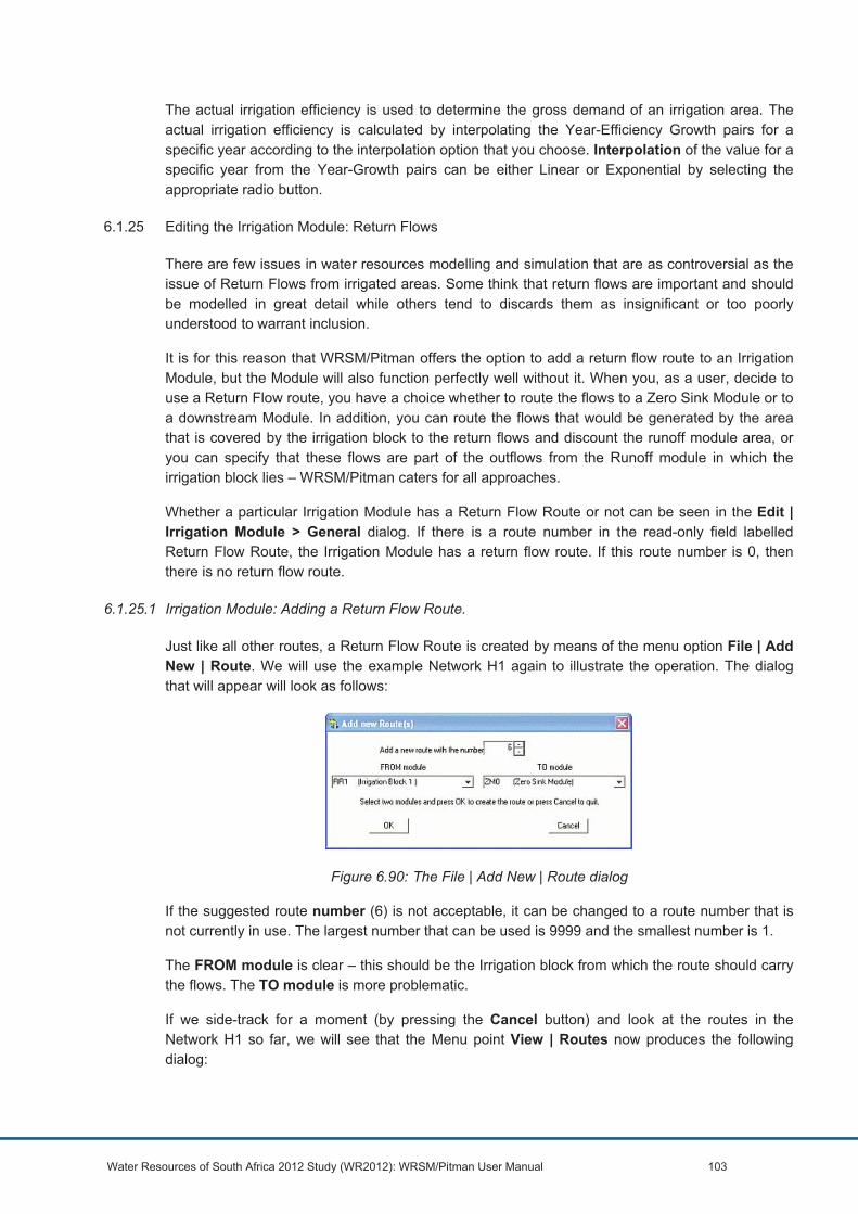
Water Resources of South Africa 2012 Study (WR2012): WRSM/Pitman User Manual 103
The actual irrigation efficiency is used to determine the gross demand of an irrigation area. The actual irrigation efficiency is calculated by interpolating the Year-Efficiency Growth pairs for a specific year according to the interpolation option that you choose. Interpolation of the value for a specific year from the Year-Growth pairs can be either Linear or Exponential by selecting the appropriate radio button.
6.1.25 Editing the Irrigation Module: Return Flows
There are few issues in water resources modelling and simulation that are as controversial as the issue of Return Flows from irrigated areas. Some think that return flows are important and should be modelled in great detail while others tend to discards them as insignificant or too poorly understood to warrant inclusion.
It is for this reason that WRSM/Pitman offers the option to add a return flow route to an Irrigation Module, but the Module will also function perfectly well without it. When you, as a user, decide to use a Return Flow route, you have a choice whether to route the flows to a Zero Sink Module or to a downstream Module. In addition, you can route the flows that would be generated by the area that is covered by the irrigation block to the return flows and discount the runoff module area, or you can specify that these flows are part of the outflows from the Runoff module in which the irrigation block lies – WRSM/Pitman caters for all approaches.
Whether a particular Irrigation Module has a Return Flow Route or not can be seen in the Edit | Irrigation Module > General dialog. If there is a route number in the read-only field labelled Return Flow Route, the Irrigation Module has a return flow route. If this route number is 0, then there is no return flow route.
6.1.25.1 Irrigation Module: Adding a Return Flow Route.
Just like all other routes, a Return Flow Route is created by means of the menu option File | Add New | Route. We will use the example Network H1 again to illustrate the operation. The dialog that will appear will look as follows:
Figure 6.90: The File | Add New | Route dialog
If the suggested route number (6) is not acceptable, it can be changed to a route number that is not currently in use. The largest number that can be used is 9999 and the smallest number is 1.
The FROM module is clear – this should be the Irrigation block from which the route should carry the flows. The TO module is more problematic.
If we side-track for a moment (by pressing the Cancel button) and look at the routes in the Network H1 so far, we will see that the Menu point View | Routes now produces the following dialog:
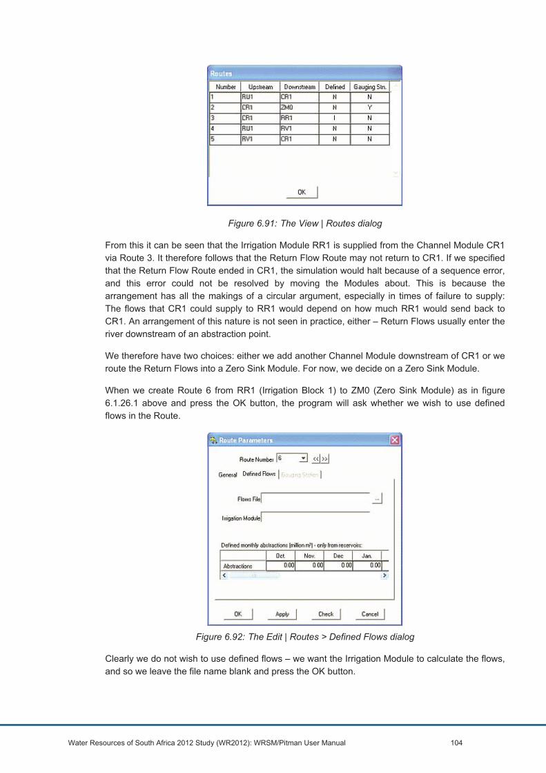
Water Resources of South Africa 2012 Study (WR2012): WRSM/Pitman User Manual 104
Figure 6.91: The View | Routes dialog
From this it can be seen that the Irrigation Module RR1 is supplied from the Channel Module CR1 via Route 3. It therefore follows that the Return Flow Route may not return to CR1. If we specified that the Return Flow Route ended in CR1, the simulation would halt because of a sequence error, and this error could not be resolved by moving the Modules about. This is because the arrangement has all the makings of a circular argument, especially in times of failure to supply: The flows that CR1 could supply to RR1 would depend on how much RR1 would send back to CR1. An arrangement of this nature is not seen in practice, either – Return Flows usually enter the river downstream of an abstraction point.
We therefore have two choices: either we add another Channel Module downstream of CR1 or we route the Return Flows into a Zero Sink Module. For now, we decide on a Zero Sink Module.
When we create Route 6 from RR1 (Irrigation Block 1) to ZM0 (Zero Sink Module) as in figure 6.1.26.1 above and press the OK button, the program will ask whether we wish to use defined flows in the Route.
Figure 6.92: The Edit | Routes > Defined Flows dialog
Clearly we do not wish to use defined flows – we want the Irrigation Module to calculate the flows, and so we leave the file name blank and press the OK button.

Water Resources of South Africa 2012 Study (WR2012): WRSM/Pitman User Manual 105
Regarding the Return Flow Route, it is not recommended to attempt to use the Return Flow Route from one Irrigation Module as the Abstraction Route for another Irrigation Module.
We have now created the Return Flow Route to Irrigation Module 1, and can edit the Return Flow parameters in Irrigation Module 1.
6.1.25.2 Editing the Irrigation Module for the Pitman irrigation model: Return Flows
The following applies if the Pitman Irrigation Model was selected for a particular Module in the dialog Edit | Irrigation Modules > General. The discussion for the same dialog for the WQT, WQT-SAPWAT or WQT Type 4 models is in section 6.1.24.3.
The menu point Edit | Irrigation Modules > Return Flows will produce the following dialog:
Figure 6.93: The Edit | Irrigation Modules > Return Flows dialog for the Pitman Irrigation model
When you use the WRSM/Pitman Irrigation Model, there is only one field that is not greyed out, and that is the field labelled Return flow as percentage of Abstraction flow. This speaks for itself.
6.1.25.3 Editing the Irrigation Module for the WQT, WQT-SAPWAT or WQT Type 4 models: Return Flows
If you have specified that the specific module should use the WQT, WQT-SAPWAT or WQT Type 4 Irrigation Models in the Edit | Irrigation Modules > General dialog, the field Return flows as percentage of the Abstraction flow will be deactivated, and the other fields activated. The dialog will therefore look as follows:

Water Resources of South Africa 2012 Study (WR2012): WRSM/Pitman User Manual 106
Figure 6.94: The Edit | Irrigation Modules > Return Flows dialog for the WQT, WQT-SAPWAT or WQT Type 4 Irrigation models
The WQT, WQT-SAPWAT and WQT Type 4 models expect a “Return Flow Factor”, a value between 0 and 1 instead of a percentage of the abstraction flows as in the case of the WRSM/Pitman Irrigation model. These two factors are not related and you are referred to (Allen et al., 1988) for further details. The return flow factor for WQT is the proportion of the soil moisture returned in each month. The default value of 0.02 should give reasonable results. Note that the “Year and Return Flow growth” grid is the same for both WQT and WQT Type 4 methodologies.
For WQT, There are two options where the “Return Flow Type” is concerned – either Net return flows or Total return flows. For WQT Type 4 the default is always to Net Return Flows.
For WQT where “Net return flows” are specified, the flows that are generated naturally by the area under irrigation are added to the outflows of the Runoff Module in which the irrigation area lies. All that is placed in the 'return flows' is the flow that is left over from the flows that enter the irrigation block via the abstraction route. In this case, the area of the Runoff module is NOT reduced.
For WQT where “Total Return Flows” are specified, the flows that are generated naturally by the area that is occupied by the irrigation area are added to the 'Net' return flows. At the same time, the area of the Runoff Module in which the irrigation area lies is reduced by the area of the irrigation block.
The net return flow is the default setting and should be used in virtually all cases. The total return flow is the sum of the natural return flow (baseflow) and the irrigated area return flow and would be of interest to the user who is also analysing water quality.
In the final analysis, the flows that are generated by the two methods are very similar, but there are subtle differences, especially in times of failure of supply. For more detailed notes on these differences, see Knowledge Base Article J6 in section 6.5.3 .

Water Resources of South Africa 2012 Study (WR2012): WRSM/Pitman User Manual 107
In addition, in the WQT, WQT-SAPWAT or WQT Type 4 models, the user must specify “Return Flow Growths”. At least two Year/Return Flow Growth value pairs must be added in the dialog, even if there is no growth. If there is no growth, the growth must be set to 1.00. A value of less than 1.00 (but greater than 0) constitutes a reduction in the return flow factor, and a value over 1.00 is an increase in the return flow factor.
The first year-value should in or before the first year of the simulation and the last year value should be on or after the last year of simulation. As in the case of all year/growth pairs, you add a value by changing it in the input mask, and then pressing the Add button. To change an existing pair, either enter it anew of click on one of the values of a pair in the list. The value pair will then be put in the input mask for editing. When editing is completed, pressing the Add button transfers the year and value to its rightful place in the list. Up to 10 year/Return Flow Growth factors can be entered for every Module.
The Return Flow Growth for a particular year is interpolated during simulation. The Interpolation type, either Linear or Exponential can be determined by clicking on the radio button of your choice.
6.1.25.4 Editing the Irrigation Module for the WQT Type 4 models: Capacity
This is only used for the WQT Type 4 method. This dialogue is used where there is a limitation of a pipeline or canal to supply water to irrigated areas. It can be varied over years. The dialog looks as follows:
Figure 6.95: The Edit | Irrigation Modules > Capacity dialog for the WQT Type 4 Irrigation models.
6.1.26 The Mining Module
6.1.26.1 Adding further Modules: The Mining Module
The following is a general description of what the mining module covers.
A mine can impact on a catchment in the following ways:-
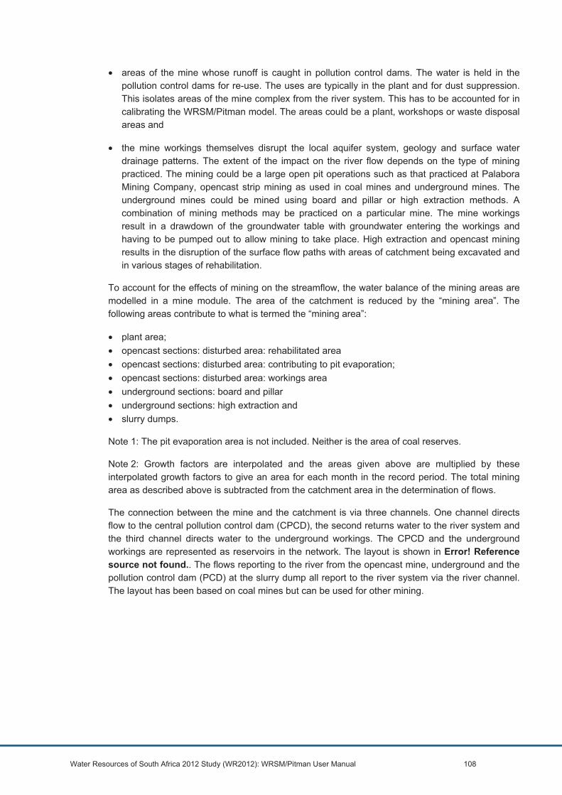
Water Resources of South Africa 2012 Study (WR2012): WRSM/Pitman User Manual 108
• areas of the mine whose runoff is caught in pollution control dams. The water is held in the pollution control dams for re-use. The uses are typically in the plant and for dust suppression. This isolates areas of the mine complex from the river system. This has to be accounted for in calibrating the WRSM/Pitman model. The areas could be a plant, workshops or waste disposal areas and
• the mine workings themselves disrupt the local aquifer system, geology and surface water drainage patterns. The extent of the impact on the river flow depends on the type of mining practiced. The mining could be a large open pit operations such as that practiced at Palabora Mining Company, opencast strip mining as used in coal mines and underground mines. The underground mines could be mined using board and pillar or high extraction methods. A combination of mining methods may be practiced on a particular mine. The mine workings result in a drawdown of the groundwater table with groundwater entering the workings and having to be pumped out to allow mining to take place. High extraction and opencast mining results in the disruption of the surface flow paths with areas of catchment being excavated and in various stages of rehabilitation.
To account for the effects of mining on the streamflow, the water balance of the mining areas are modelled in a mine module. The area of the catchment is reduced by the “mining area”. The following areas contribute to what is termed the “mining area”:
• plant area; • opencast sections: disturbed area: rehabilitated area • opencast sections: disturbed area: contributing to pit evaporation; • opencast sections: disturbed area: workings area • underground sections: board and pillar • underground sections: high extraction and • slurry dumps.
Note 1: The pit evaporation area is not included. Neither is the area of coal reserves.
Note 2: Growth factors are interpolated and the areas given above are multiplied by these interpolated growth factors to give an area for each month in the record period. The total mining area as described above is subtracted from the catchment area in the determination of flows.
The connection between the mine and the catchment is via three channels. One channel directs flow to the central pollution control dam (CPCD), the second returns water to the river system and the third channel directs water to the underground workings. The CPCD and the underground workings are represented as reservoirs in the network. The layout is shown in Error! Reference source not found.. The flows reporting to the river from the opencast mine, underground and the pollution control dam (PCD) at the slurry dump all report to the river system via the river channel. The layout has been based on coal mines but can be used for other mining.
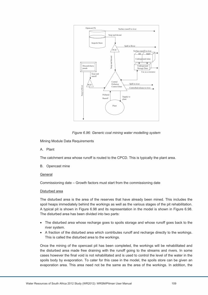
Water Resources of South Africa 2012 Study (WR2012): WRSM/Pitman User Manual 109
Figure 6.96: Generic coal mining water modelling system
Mining Module Data Requirements
A. Plant
The catchment area whose runoff is routed to the CPCD. This is typically the plant area.
B. Opencast mine
General
Commissioning date – Growth factors must start from the commissioning date
Disturbed area
The disturbed area is the area of the reserves that have already been mined. This includes the spoil heaps immediately behind the workings as well as the various stages of the pit rehabilitation. A typical pit is shown in Figure 6.98 and its representation in the model is shown in Figure 6.98. The disturbed area has been divided into two parts:
• The disturbed area whose recharge goes to spoils storage and whose runoff goes back to the river system.
• A fraction of the disturbed area which contributes runoff and recharge directly to the workings. This is called the disturbed area to the workings.
Once the mining of the opencast pit has been completed, the workings will be rehabilitated and the disturbed area made free draining with the runoff going to the streams and rivers. In some cases however the final void is not rehabilitated and is used to control the level of the water in the spoils body by evaporation. To cater for this case in the model, the spoils store can be given an evaporation area. This area need not be the same as the area of the workings. In addition, the
Plant
Polluted
RunoffSupply toplant
CentralPollutionControl Dam
Discard/slurryponds
PCDSe
ep to
Riv
er
Seep andrunoff
Surface runoff to river
Seep and decant
Opencast Pit
Inspoils Store
PCD
Spill to River
Seep
and
dec
ant
Surface runoff to river
Underground mine
UndergroundStorage Dam
Spill to river
Controlled release to river
Use as a resource
HE B&P

Water Resources of South Africa 2012 Study (WR2012): WRSM/Pitman User Manual 110
final void evaporation area may receive surface runoff. To allow for this, the disturbed area to workings can contribute surface runoff to the pit after closure.
Figure 6.97: Typical opencast pit layout
Figure 6.98: Schematic showing model representation in opencast pit
The areas of the pit change over time as the mine progresses. Growth factors have therefore been included in the model to allow for the change in the different areas over time. The mine plan is used to determine the change in areas over time.
The water entering the pit is calculated using the pit area, the rainfall depth and a recharge factor. A recharge factor is entered for each month of the year for each of the areas. For typical spoils and pit rehabilitation, the recharge factor is between 12% and 14%. If the pit is not well rehabilitated or the rehabilitation has lagged behind, the recharge could be as high as 26%.
Workings
Normally 40m wide strips and two lines of inspoils heaps.
workings
SpoilsRehabilitated spoils
workings
SpoilsRehabilitated spoils
Undisturbed Area
AUD
Disturbed Area
ADA
Disturbed Workings
ADAW
Workings
AW
Rese
rve
Are
a A
RES
QUDA
QDA
RDA Inspoils Dam
QSE
EP+Q
DEC
PC Dam
QW
Closure
AW=0
To Central PCD if VFPC=0
QSPILL
QDAWRDAW

Water Resources of South Africa 2012 Study (WR2012): WRSM/Pitman User Manual 111
Pit Evaporation
This normally applies to the closure state of the pit where an evaporation area is engineered into the rehabilitation of the pit. This is normally in the final void. The evaporation area is sized so as to evaporate the pit water make and keep the pit in balance.
Rehabilitated
The rehabilitation of the spoil heaps involves flattening of the heaps and the application of a soil cover to the rehabilitated spoils. The recharge through the soil cover is stored in the spoils under the soil cover. This is called the inspoils store. The water accumulates in the inspoils store. The water level rises in the inspoils store until it reaches the weathered where seepage will occur through the weathered zone. If the water level rises further then the pit will ultimately decant. A rehabilitated pit is shown in Figure 6.99 with the water level having reached the seepage zone.
Figure 6.99: Rehabilitated pit with the water level at the weathered zone.
Inspoils Seep volume
The volume of water stored in the spoils at which seepage occurs. The model tracks the volume stored in the Inspoils store when the volume exceeds the Inspoils seepage volume, then seepage occurs through the weathered zone. The inspoils seepage volume can change over time so growth factors have been included in the model to allow for this.
Inspoils Decant
This is similar to the seepage volume. This is the volume at which the pit starts to decant. This is similar to a spill from a reservoir.
Underground Mines
In bord and pillar mining, columns of coal are left in the workings to support the roof. Normally about 40% to 50% of the coal is mined with the rest left behind as pillars. There is limited surface subsidence and the recharge is typically 1% to 3% which is similar to natural conditions.
High extraction mining is when about 90% of the coal is mined and roof of the workings are allowed to collapse. The mining void is then filled with roof material and the collapse is reflected at surface as a corrugation. The strata overlying the workings cracks and the cracks can go through to the surface. The cracks on surface intercept runoff from upstream catchments which then reports to the workings. The model allows for a runoff factor to adjust the runoff that can be expected from the mining area. An upstream mining area is also specified in the model input. This is the area whose runoff passes over the area mined using high extraction. A factor is used to

Water Resources of South Africa 2012 Study (WR2012): WRSM/Pitman User Manual 112
determine the fraction of the runoff from the upstream area whose runoff can be intercepted by the cracks and report to the workings. Recharge factors of about 5%-8% can be used for high extraction mining. The layout for the underground mining is shown in Figure 6.100 .
Figure 6.100: Schematic representation of underground mine used in model
Slurry dump
When a mine has a slurry dump, the slurry dump area is affectively isolated from the catchment by PCD. The slurry dump consists of the dump and a local pollution control dam with the spill from the local pollution control dam reporting to the CPCD. The inflow to the local pollution control dam at the slurry dump is the runoff from the dump and a fraction of the seepage from the bottom of the dumps. The balance of the seepage reports to the river via the river channel. The schematic of the slurry dump is shown in Figure 6.101 Error! Reference source not found..
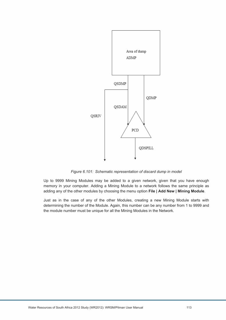
Water Resources of South Africa 2012 Study (WR2012): WRSM/Pitman User Manual 113
Figure 6.101: Schematic representation of discard dump in model
Up to 9999 Mining Modules may be added to a given network, given that you have enough memory in your computer. Adding a Mining Module to a network follows the same principle as adding any of the other modules by choosing the menu option File | Add New | Mining Module.
Just as in the case of any of the other Modules, creating a new Mining Module starts with determining the number of the Module. Again, this number can be any number from 1 to 9999 and the module number must be unique for all the Mining Modules in the Network.

Water Resources of South Africa 2012 Study (WR2012): WRSM/Pitman User Manual 114
6.1.26.2 Editing the Mining Module, the General dialog
Once the question of the number is settled, and the OK button is pressed, the program will automatically open the dialog:
Figure 6.102: The Edit | Mining Module > General dialog for the WRSM/Pitman Mining Module
Here we fill in the name of the mining property which is represented by the Mining Module and also the “Runoff Module in which the mining module lies”. Due to the fact that the Mining Module will reduce the area of the Runoff Module in which it lies, this parameter is of some importance.

Water Resources of South Africa 2012 Study (WR2012): WRSM/Pitman User Manual 115
6.1.26.3 Editing the Mining Module, the Climate dialog
The Climate dialog for the Mining Module bears a strong resemblance to all other previous climate screens and looks as follows:
Figure 6.103: The Edit | Mining Module > Climate dialog for the WRSM/Pitman Mining Module
Here we add the Rainfile name and the MAP and either enter the 12 required monthly Evaporations, or copy them from other, existing Mining Modules.
6.1.26.4 Editing the Mining Module, Outflow Routes and the Outflow dialog.
Before we can set the outflow routes in the Mining Module, we first have to define the outflow routes that leave the Mining Module.
For this we need to close the Mining Module dialog temporarily by pressing the Apply Button to save all the data that we have entered before, and then pressing the Cancel Button. If we press the OK button at this stage, the Module will be checked and found lacking in outflow routes and declared invalid.
An outflow route is added to a Mining Module in exactly the same manner as an outflow route is added to any other Module.
It should be borne in mind that the Mining Module will require at least 2 outflow routes, namely: one route to carry outflows from the Mining Module directly into a Channel Reach and one route to carry outflows from the Mining Module to a Central Pollution Control Dam.
Note that the Central Pollution Control dam is a Reservoir Module that is situated outside of the Mining Property and should not be confused with the myriad of small pollution control dams that can be placed at the outflows of almost every section within the Mining Module. All these small pollution control dams spill into a single outflow route that drains into the external Central Pollution Control Dam.
Note also that if the user has an underground section, the outflow route from that section to the river should not be the same as the outflow route to the river for the mine as a whole.

Water Resources of South Africa 2012 Study (WR2012): WRSM/Pitman User Manual 116
If you have not yet created this Central Pollution Control Dam in your Network, you may wish to create that Reservoir Module before you add the outflow routes that emerge from the Mining Module. You could also create the routes to drain temporarily to Zero Modules and redefine them later but this is not advised. The second route will lead to 'a river' – for this neither of the routes should carry defined flows.
Once the outflow routes exist, you can return to the Edit | Mining Modules > Outflow dialog:
Figure 6.104: The Edit | Mining Module > Outflow dialog for the WRSM/Pitman Mining Module
If a mine has a plant, then details can be entered in the following dialog:
Figure 6.105: The Edit | Mining Module > Plant dialog for the WRSM/Pitman

Water Resources of South Africa 2012 Study (WR2012): WRSM/Pitman User Manual 117
Mining Module
There are three types of mine that can be chosen from the Edit|Mining Modules > Sections dialogue, namely: Opencast section, Underground section and Slurry Pond/Dump areas. A mine can have a number of these sections in combination or none if that is the case. Each of these mine types has a further set of dialogues. These dialogues will not be shown as there are quite a number of them, only the three main mine types have been shown below in Figures 6.106 to 6.108.
Figure 6.106: The Edit | Mining Module | Section > Opencast Section dialog for the WRSM/Pitman
Mining Module
Figure 6.107: The Edit | Mining Module | Section > Underground Section dialog for the WRSM/Pitman Mining Module

Water Resources of South Africa 2012 Study (WR2012): WRSM/Pitman User Manual 118
Figure 6.108: The Edit | Mining Module | Section > Dump Area Section dialog for the WRSM/Pitman Mining Module
6.1.27 Saving Simulation Results – Flows and Storages.
Once a simulation has been run successfully, the flows time series for any of the routes can be saved to file(s), as can the time series if the storages in the reservoirs.
6.1.27.1 Saving Route Flows
A route flow can be saved by choosing the menu point File | Save | Route Flows. When you choose this menu point, the following dialog will appear:
Figure 6.109: The File | Save | Route Flows dialog
By clicking on the arrow on the right hand side of the field labelled Route Number, a list-box will open with all the Routes in the Network from which you can choose the route for which you wish to save the flows.
When you have selected a Route, the read-only fields labelled “From Module” and “To Module” will show the modules that are upstream and downstream of the route. These field are there only as reminders.

Water Resources of South Africa 2012 Study (WR2012): WRSM/Pitman User Manual 119
Depending on the route that you have selected, one or more of the radio-button points Simulated, Demands and Shortages will become active in the group box Flows to Save. In most cases, the Simulated choice will be active. The Demands choice will only be active if the route carries a Demand, for example the demands that are generated in an abstraction Route by an Irrigation Module.
When the Demands choice is active, the Shortages option will also be active. By means of this choice, you can save the difference between the demand and the flows that were actually supplied.
Once you have selected one of the Flows to Save radio buttons, a file name for the file that will be created will be suggested. The File Name that is suggested in Network H1 will always have the form:
H1 – the Network code followed by
RQ – for Route Flows followed by (for example)
3 – for the Route number
If you select the Simulated flows option, the file will have the suffix “.ANS”.
If you select the Demands option, the file name will end in “.DEM” and
If the Shortages option was chosen, the file name will always end in “.SHO”
The program will always suggest that the files be saved in the Output folder for the network.
The suggested naming convention is not binding, and you can change the names and the directories at will.
6.1.27.2 Saving Reservoir Storage States
The reservoir storage state time series can be saved by means of choosing the menu point File | Save | Reservoir Storages. This will produces the following dialog:
Figure 6.110: The File | Save | Reservoir Storages dialog
By clicking on the arrow next to the field labelled Reservoir, a list box will open from where you can select the Reservoir that you wish to store. When you have selected a reservoir, a File Name will automatically be suggested. The name of the file will have the form:
H1 for the Network code, followed by
RV to signify that the file contains reservoir data, followed by
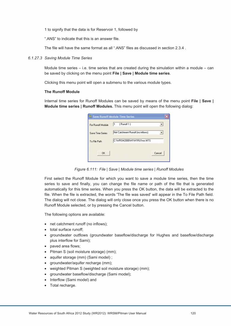
Water Resources of South Africa 2012 Study (WR2012): WRSM/Pitman User Manual 120
1 to signify that the data is for Reservoir 1, followed by
“.ANS” to indicate that this is an answer file.
The file will have the same format as all “.ANS” files as discussed in section 2.3.4 .
6.1.27.3 Saving Module Time Series
Module time series – i.e. time series that are created during the simulation within a module – can be saved by clicking on the menu point File | Save | Module time series.
Clicking this menu point will open a submenu to the various module types.
The Runoff Module
Internal time series for Runoff Modules can be saved by means of the menu point File | Save | Module time series | Runoff Modules. This menu point will open the following dialog:
Figure 6.111: File | Save | Module time series | Runoff Modules
First select the Runoff Module for which you want to save a module time series, then the time series to save and finally, you can change the file name or path of the file that is generated automatically for this time series. When you press the OK button, the data will be extracted to the file. When the file is extracted, the words 'The file was saved' will appear in the To File Path field. The dialog will not close. The dialog will only close once you press the OK button when there is no Runoff Module selected, or by pressing the Cancel button.
The following options are available:
• net catchment runoff (no inflows); • total surface runoff; • groundwater outflows (groundwater baseflow/discharge for Hughes and baseflow/discharge
plus interflow for Sami); • paved area flows; • Pitman S (soil moisture storage) (mm); • aquifer storage (mm) (Sami model) ; • groundwater/aquifer recharge (mm); • weighted Pitman S (weighted soil moisture storage) (mm); • groundwater baseflow/discharge (Sami model); • Interflow (Sami model) and • Total recharge.
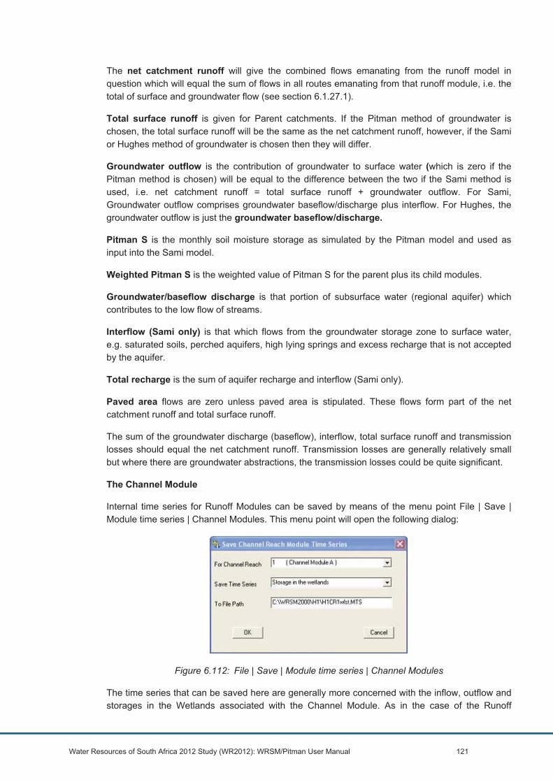
Water Resources of South Africa 2012 Study (WR2012): WRSM/Pitman User Manual 121
The net catchment runoff will give the combined flows emanating from the runoff model in question which will equal the sum of flows in all routes emanating from that runoff module, i.e. the total of surface and groundwater flow (see section 6.1.27.1).
Total surface runoff is given for Parent catchments. If the Pitman method of groundwater is chosen, the total surface runoff will be the same as the net catchment runoff, however, if the Sami or Hughes method of groundwater is chosen then they will differ.
Groundwater outflow is the contribution of groundwater to surface water (which is zero if the Pitman method is chosen) will be equal to the difference between the two if the Sami method is used, i.e. net catchment runoff = total surface runoff + groundwater outflow. For Sami, Groundwater outflow comprises groundwater baseflow/discharge plus interflow. For Hughes, the groundwater outflow is just the groundwater baseflow/discharge.
Pitman S is the monthly soil moisture storage as simulated by the Pitman model and used as input into the Sami model.
Weighted Pitman S is the weighted value of Pitman S for the parent plus its child modules.
Groundwater/baseflow discharge is that portion of subsurface water (regional aquifer) which contributes to the low flow of streams.
Interflow (Sami only) is that which flows from the groundwater storage zone to surface water, e.g. saturated soils, perched aquifers, high lying springs and excess recharge that is not accepted by the aquifer.
Total recharge is the sum of aquifer recharge and interflow (Sami only).
Paved area flows are zero unless paved area is stipulated. These flows form part of the net catchment runoff and total surface runoff.
The sum of the groundwater discharge (baseflow), interflow, total surface runoff and transmission losses should equal the net catchment runoff. Transmission losses are generally relatively small but where there are groundwater abstractions, the transmission losses could be quite significant.
The Channel Module
Internal time series for Runoff Modules can be saved by means of the menu point File | Save | Module time series | Channel Modules. This menu point will open the following dialog:
Figure 6.112: File | Save | Module time series | Channel Modules
The time series that can be saved here are generally more concerned with the inflow, outflow and storages in the Wetlands associated with the Channel Module. As in the case of the Runoff
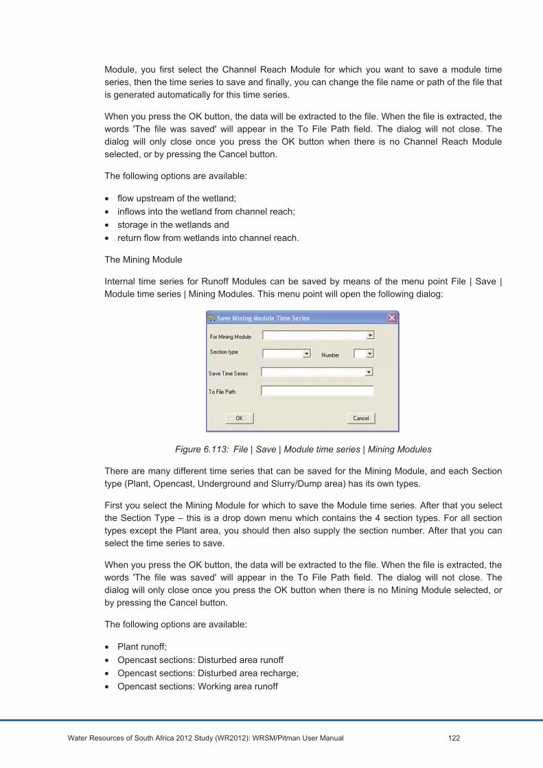
Water Resources of South Africa 2012 Study (WR2012): WRSM/Pitman User Manual 122
Module, you first select the Channel Reach Module for which you want to save a module time series, then the time series to save and finally, you can change the file name or path of the file that is generated automatically for this time series.
When you press the OK button, the data will be extracted to the file. When the file is extracted, the words 'The file was saved' will appear in the To File Path field. The dialog will not close. The dialog will only close once you press the OK button when there is no Channel Reach Module selected, or by pressing the Cancel button.
The following options are available:
• flow upstream of the wetland; • inflows into the wetland from channel reach; • storage in the wetlands and • return flow from wetlands into channel reach.
The Mining Module
Internal time series for Runoff Modules can be saved by means of the menu point File | Save | Module time series | Mining Modules. This menu point will open the following dialog:
Figure 6.113: File | Save | Module time series | Mining Modules
There are many different time series that can be saved for the Mining Module, and each Section type (Plant, Opencast, Underground and Slurry/Dump area) has its own types.
First you select the Mining Module for which to save the Module time series. After that you select the Section Type – this is a drop down menu which contains the 4 section types. For all section types except the Plant area, you should then also supply the section number. After that you can select the time series to save.
When you press the OK button, the data will be extracted to the file. When the file is extracted, the words 'The file was saved' will appear in the To File Path field. The dialog will not close. The dialog will only close once you press the OK button when there is no Mining Module selected, or by pressing the Cancel button.
The following options are available:
• Plant runoff; • Opencast sections: Disturbed area runoff • Opencast sections: Disturbed area recharge; • Opencast sections: Working area runoff

Water Resources of South Africa 2012 Study (WR2012): WRSM/Pitman User Manual 123
• Opencast sections: Disturbed area that drains to workings recharge; • Opencast sections: Disturbed area that drains to workings: runoff • Opencast sections: Disturbed area that drains to workings: seepage; • Opencast sections: Disturbed area that drains to workings: decant; • Opencast sections: Pollution control dam: spillage • Opencast sections: Pollution control dam: storage • Opencast sections: Pollution control dam: month start storage; • Opencast sections: Pollution control dam: month end storage; • Opencast sections: Inspoil storage; • Underground: Runoff from upstream area; • Underground: Recharge to underground mining area; • Underground: Runoff from Board and Pillar; • Underground: Runoff from High Extraction; • Slurry dump: Surface runoff from dump; • Slurry dump: Seepage from dump; • Slurry dump: Inflow to pollution control dam; • Slurry dump: Storage in pollution control dam; • Slurry dump: Spillage from pollution control dam.
6.1.28 Converting Files
Many hydrologists make extensive use of spreadsheets to analyse their data further or to produce presentation graphics. Some may also want to import data that was produced in spreadsheets into WRSM/Pitman. For this reason, the program now features 2 small utilities to aid in this task.
The first utility converts any “WRSM2000.ANS” file to a “.CSV” (Comma Separated Value) file that can be imported into a 2 column (Year Value for 12 months) spreadsheet.
The second utility converts a “.CSV” file that was created by a 2 column spreadsheet (Year Value) to a “.ANS” file that can be read by WRSM/Pitman.
These utilities can be accessed by means of the Menu points File | Convert | .ANS to .CSV and File | Convert | .CSV to .ANS.
The dialogs only differ in the choice of input and output file type and speak for themselves.
Figure 6.114: File | Convert | “.ANS” to “.CSV” and File | Convert | “.CSV” to “.ANS”
6.1.29 Exit the program and Closing the Network
When you exit WRSM/Pitman, either by means of the menu point File | Exit WRSM/Pitman or by a click on the door button in the tool bar, the program will check automatically whether the

Water Resources of South Africa 2012 Study (WR2012): WRSM/Pitman User Manual 124
Network on which you were working was changed since it was last saved. If the Network was changed but not saved, the message shown in the following figure will appear.
Figure 6.115: The network not saved dialog
Pressing the No button will take you back to the program from where you can save the network before closing the program again.
Pressing the Yes button will skip the saving of the Network, but the program will then carry on to check whether any of the modules in the Network that you were working on was changed but not saved. If such a module is found, the message shown in the following figure will appear.
Figure 6.116: The “do you want to save” Dialog
The program goes from the point of view that you may wish to undo the adding or deleting of a module or route in the Network, but that you still might wish to keep the changes that you made in the individual modules, or the data that you typed into that Module.
Once all the modules that were changed were saved (or not, as determined by you, the user) the program will close.
Closing the Network by means of the menu point File | Close Network will also check for changes in the Network and in the Modules, but once all the data is cleared out of memory, the program itself does not close. It will remain open, and the words Network: None will be visible at the bottom left of the window. From there, you can either open an existing Network, or create a new one as described in 6.1.2.
6.2 More Advanced Operations and Configurations
6.2.1 Changing the Simulation Period
Once a Network is loaded, the simulation period can no longer be changed. This is because the WRSM/Pitman allocates just enough memory and loads just that data that it really needs in order to use the memory space in your machine as effectively as possible. Saving on memory space will allow you to create very large networks, even on machines with smaller amounts of memory.

Water Resources of South Africa 2012 Study (WR2012): WRSM/Pitman User Manual 125
To change the simulation period of a Network, one has to close the network temporarily (saving it, if necessary) and then open it again.
When we use the menu point File | Open Network, and we select our example network “C:\WRSM2000\H1” from the standard Open File dialog, we see the following dialog:
Figure 6.117: The Load Network File Dialog
In this dialog we can change the Result Folder, the Simulation Year Start and the Simulation Year End. You can now also change the simulation period. The only restrictions that apply are that the Start year must be before the end year and you cannot start before the year 1850 or end after the year 2100. As a further reality check, the number of years that can be simulated has been limited to 150 years.
Once you have changed the start and end dates of the simulation, the program will check whether the data that was entered in the modules, such as the year/area pairs and year/growth pairs cover the simulation period. If they do not cover the period, you will be alerted.
Where Rainfiles do not cover a portion of the period, your attention will also be drawn to that and the rainfall as percentage of MAP will be set to 0.0 for those years for which there is no data.
6.2.2 Special areas within Runoff Modules
There are currently three different special area types that influence the runoff that will be generated by a Runoff Module: Paved Area, Afforested Area and Alien Vegetation.
It is self-evident that the sum total area of all special area types for any given year within the simulation period may not exceed the total area of the catchment in which they lie. WRSM/Pitman will check the data of any Runoff Module that contains special areas to ensure that this is the case.
In WRSM/Pitman, the research carried out on afforestation (D F Scott et al., 1997), Gush and on alien vegetation (Le Maitre et al., 2001) has been applied.
6.2.2.1 Afforestation
In WRSM/Pitman both Afforestation and Alien Vegetation are dealt with in the Runoff Module. In order to specify the characteristics of an afforested area within a particular Runoff Module, the dialog Edit | Runoff Module > Afforestation should be selected.
In Runoff Module 1, the only Runoff Module that we have in our Network so far, this dialog would look as follows:
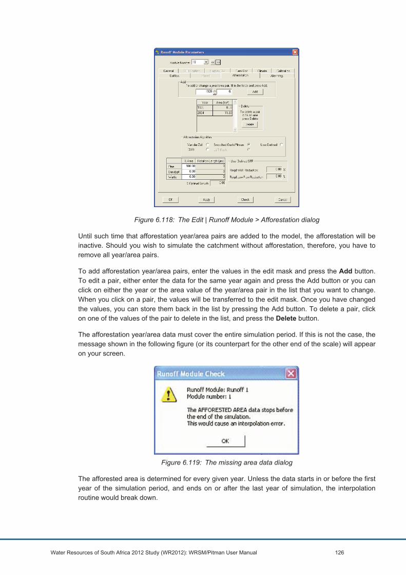
Water Resources of South Africa 2012 Study (WR2012): WRSM/Pitman User Manual 126
Figure 6.118: The Edit | Runoff Module > Afforestation dialog
Until such time that afforestation year/area pairs are added to the model, the afforestation will be inactive. Should you wish to simulate the catchment without afforestation, therefore, you have to remove all year/area pairs.
To add afforestation year/area pairs, enter the values in the edit mask and press the Add button. To edit a pair, either enter the data for the same year again and press the Add button or you can click on either the year or the area value of the year/area pair in the list that you want to change. When you click on a pair, the values will be transferred to the edit mask. Once you have changed the values, you can store them back in the list by pressing the Add button. To delete a pair, click on one of the values of the pair to delete in the list, and press the Delete button.
The afforestation year/area data must cover the entire simulation period. If this is not the case, the message shown in the following figure (or its counterpart for the other end of the scale) will appear on your screen.
Figure 6.119: The missing area data dialog
The afforested area is determined for every given year. Unless the data starts in or before the first year of the simulation period, and ends on or after the last year of simulation, the interpolation routine would break down.

Water Resources of South Africa 2012 Study (WR2012): WRSM/Pitman User Manual 127
Clearly the area under afforestation can never be greater than the total area of the catchment. The total area covered by Afforestation, Alien Vegetation and Paved area may also not exceed the total area of the catchment.
As can be seen from the previous dialog, there are five afforestation models to choose from as follows: the Van der Zel model, the CSIR model the Smoothed Gush/Pitman, the User Defined and LUT Gush (not active at this stage). Newly created Runoff Modules will default to the CSIR algorithm. The Van der Zel Model is the model that was used in all versions of WRSM90 and WRSM/Pitman before version 2. When the program reads a Runoff Module file that was created with a version prior to Version 2, the Van der Zel algorithm will be used – provided, of course, that afforestation data was present in the module.
You can choose which of the five afforestation models will be used for a specific Runoff Module by selecting the required one from the radio buttons. When you choose the Van der Zel model, the dialog fields below the radio buttons (Pine, Eucalyptus, Wattle, etc.) will remain greyed out. These fields are inactive because the Van der Zel algorithm does not require any of the data in those fields.
When you specify the CSIR model, the program also requires the percentage of the afforested area and rotation lengths (in years) for the three afforestation classes that can be modelled: Pine, Eucalyptus and Wattle. The percentage of optimal area is also required in the field labelled % Optimal Growth.
The CSIR algorithm calculates the reduction in flow from a catchment as a result of the three afforestation classes. In the CSIR model, lookup tables of appropriate values for annual and low flow reductions based on the percentage of optimal area are used along with empirical equations.
The Van der Zel model was used exclusively in WRSM90 and Version 1.x of WRSM/Pitman. This algorithm reduces the runoff from a catchment 'at source' by reducing the rainfall on the catchment by the amount that is intercepted by the afforestation.
Note that when you swop from one afforestation model to the other, you must press the Apply button before the change becomes active. Please refer to Section 6.2.2.3 (Streamflow Reduction Areas) for an alternative (and improved) procedure for modelling the impact of afforestation and alien vegetation.
6.2.2.2 Alien Vegetation
In order to specify the characteristics of Alien Vegetation in a particular Runoff Module, the dialog Edit | Runoff Module > Alien Veg. should be selected.
In Runoff Module 1, the only Runoff Module that we have in our Network so far, this dialog would look as follows:

Water Resources of South Africa 2012 Study (WR2012): WRSM/Pitman User Manual 128
Figure 6.120:The Edit | Runoff Module | Alien Vegetation dialog
The Alien Vegetation stream flow reduction model will only become active when Year/area data for Alien Vegetation is added to the module.
To add Alien Vegetation year/area pairs, enter the values in the edit mask and press the Add button. To edit a pair, either enter the data for the same year again and press the Add button or you can click on either the year or the area value of the year/area pair in the list that you want to change. When you click on a pair, the values will be transferred to the edit mask. Once you have changed the values, you can store them back in the list by pressing the Add button. To delete a pair, click on one of the values of the pair to delete in the list, and press the Delete button.
The Alien Vegetation year/area data must cover the entire simulation period. If this is not the case, the module will issue a warning. The Alien Vegetation area is determined for every given year in the simulation. Unless the data starts on or before the first year of the simulation period, and ends on or after the last year of simulation, the interpolation routine would break down.
Clearly the area that is covered by Alien Vegetation can never be greater than the total area of the catchment. The total area covered by Afforestation, Alien Vegetation and Paved area may also not exceed the total area of the catchment.
A model for the reduction in stream flow as a result of Alien Vegetation was not available in either WRSM90 or any version of WRSM/Pitman prior to version 2.0 .
There are three classes of alien vegetation, namely: Tall Trees, Medium Trees and Tall Shrubs. The percentage of the overall alien vegetation area for each of these classes is required in the field labelled %Area and the corresponding age (in years) in the Age field. Clearly the total percentage area should add up to 100%, but the program will check that. As in the case of afforestation, the “percentage of optimal area growth” is also required.
Reduction in flow for alien vegetation takes into account the biomass (based on age) of the three classes of alien vegetation. Long lag and short lag relationships are dealt with as well as with the percentage of optimal area for determining annual and low flow reductions in flow for each type of lag by means of empirical equations.
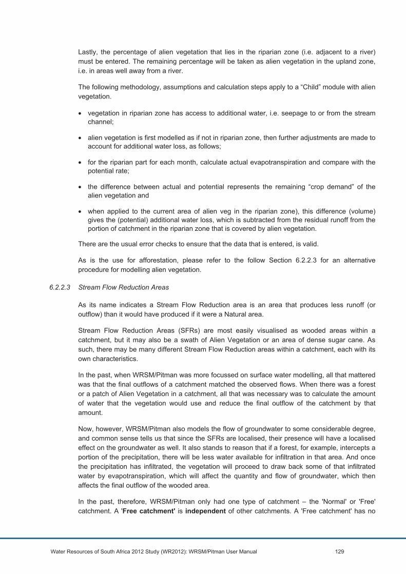
Water Resources of South Africa 2012 Study (WR2012): WRSM/Pitman User Manual 129
Lastly, the percentage of alien vegetation that lies in the riparian zone (i.e. adjacent to a river) must be entered. The remaining percentage will be taken as alien vegetation in the upland zone, i.e. in areas well away from a river.
The following methodology, assumptions and calculation steps apply to a “Child” module with alien vegetation.
• vegetation in riparian zone has access to additional water, i.e. seepage to or from the stream channel;
• alien vegetation is first modelled as if not in riparian zone, then further adjustments are made to account for additional water loss, as follows;
• for the riparian part for each month, calculate actual evapotranspiration and compare with the potential rate;
• the difference between actual and potential represents the remaining “crop demand” of the alien vegetation and
• when applied to the current area of alien veg in the riparian zone), this difference (volume) gives the (potential) additional water loss, which is subtracted from the residual runoff from the portion of catchment in the riparian zone that is covered by alien vegetation.
There are the usual error checks to ensure that the data that is entered, is valid.
As is the use for afforestation, please refer to the follow Section 6.2.2.3 for an alternative procedure for modelling alien vegetation.
6.2.2.3 Stream Flow Reduction Areas
As its name indicates a Stream Flow Reduction area is an area that produces less runoff (or outflow) than it would have produced if it were a Natural area.
Stream Flow Reduction Areas (SFRs) are most easily visualised as wooded areas within a catchment, but it may also be a swath of Alien Vegetation or an area of dense sugar cane. As such, there may be many different Stream Flow Reduction areas within a catchment, each with its own characteristics.
In the past, when WRSM/Pitman was more focussed on surface water modelling, all that mattered was that the final outflows of a catchment matched the observed flows. When there was a forest or a patch of Alien Vegetation in a catchment, all that was necessary was to calculate the amount of water that the vegetation would use and reduce the final outflow of the catchment by that amount.
Now, however, WRSM/Pitman also models the flow of groundwater to some considerable degree, and common sense tells us that since the SFRs are localised, their presence will have a localised effect on the groundwater as well. It also stands to reason that if a forest, for example, intercepts a portion of the precipitation, there will be less water available for infiltration in that area. And once the precipitation has infiltrated, the vegetation will proceed to draw back some of that infiltrated water by evapotranspiration, which will affect the quantity and flow of groundwater, which then affects the final outflow of the wooded area.
In the past, therefore, WRSM/Pitman only had one type of catchment – the 'Normal' or 'Free' catchment. A 'Free catchment' is independent of other catchments. A 'Free catchment' has no

Water Resources of South Africa 2012 Study (WR2012): WRSM/Pitman User Manual 130
influence on any other catchment and cannot be influenced – or take any “orders” – from any other catchment either.
In order to model the localised effects of SFRs, we have come up with the idea of an 'encompassing catchment' (i.e. the total quaternary catchment) within which smaller 'SFR sub-catchments' take up space, produce less runoff than under Natural conditions and so reduce the total runoff of the 'encompassing catchment'.
Because they are part of the 'encompassing catchment', the SFR sub-catchments share most of the simulation parameters with the 'encompassing catchment' in which they lie.
Conversely, the area of the 'encompassing catchment' would grow and shrink as the areas of the 'SFR sub-catchments' within its borders grow and shrink.
Somehow, the term 'encompassing catchment' does not roll off the tongue easily, and 'SFR sub-catchment' is also longwinded and sounds 'independent'. SFR-sub-catchments are not independent – if a simulation parameter is changed in the 'encompassing catchment', it must also be changed in any 'SFR sub-catchment' that lies within its borders.
To show that an 'encompassing catchment' is in charge – at least as far as simulation parameters are concerned – we decided to call such a catchment a 'Parent catchment'.
Since all 'SFR sub-catchments' within a Parent catchment are subordinate to that Parent catchments, we decided to call an 'SFR sub-catchment' a 'Child catchment'.
If a catchment is neither a Parent nor a Child, we call this catchment a 'Free catchment'
The Parent and Child nomenclature describes the way in which the catchments types act, react and interact with one another very well, and should therefore be taken with a sense of humour.
A) All catchments are created as 'Free' catchments.
A Free catchment is neither a Parent nor a Child. A Free catchment has the potential to become either a Parent or a Child.
B) Any Free catchment can be 'elevated' to the status of Parent catchment.
A Parent catchment can capture Child catchments to become part of itself. A Parent catchment can free any Child catchment that it does not need any more. A Parent catchment cannot be captured by another Parent catchment.
C) A Parent catchment can be told to 'capture' a Free catchment as a Child:
A Child cannot be captured by any other Parent. A Child takes on parameters of its Parent only. A Child only runs when told to do so by its Parent. A Child contributes its Runoff to the outflow of the Parent. When freed by its Parent, a Child reverts to a 'Free' catchment.
D) A Parent catchment can be changed to a 'Free' catchment only once it has freed all its Children.
Although, for now, our Child catchments only deal with Stream Flow Reduction areas, this concept could be broadened later to cover Stream Flow Enhancing areas (such as Paved areas) as well, since these areas, too, have an influence on groundwater.

Water Resources of South Africa 2012 Study (WR2012): WRSM/Pitman User Manual 131
Example Discussion
The way in which Parent and Child catchments are used in WRSM/Pitman is best illustrated by means of an example.
Since this is a fairly advanced topic, we will assume that you have experience in how to set up a Network and know the meaning and properties of Routes and Runoff Modules.
We will use a pre-existing Network (H1) and illustrate the actions to be taken there. Clearly one has to start WRSM/Pitman and load the Network H1 by means of the menu choice File | Open Network. When we check the Runoff Modules, by means of View | Runoff Modules we see that the Network already contains 3 Runoff Modules – Numbers 1, 7 and 12. All three of these Runoff modules are 'Free' Runoff modules. To see the status of a Runoff Module, we use the option Edit | Runoff Modules > General. For Runoff Module 1, this shows the following dialog:
Figure 6.121: Edit | Runoff Modules > General Dialog
Note that the check box behind The Module is a Parent Module is unchecked and also that the field after This Module is a Child Module to RU contains a 0. This means that the Runoff Module is neither a Parent module nor a Child Module, it is a Free module.
If the user has information that there is an afforested area in this catchment and that a portion of the catchment actually produces far less outflow than it would do under natural circumstances because someone started planting sugarcane there, use (say) the Sami Groundwater Model to simulate the groundwater flows and because of this we use the SFR Parent/Child configuration to simulate this catchment.
The catchment Runoff 1 would therefore become the Parent catchment, since the afforested area and the sugar cane area lie within it. In addition, the user would need to create two Child catchments – one for the afforested area and one for the sugar cane area.
To start (and while the user has the dialog open, the order does not matter) change the Groundwater Model of Runoff Module 1 from the Pitman Model to the Sami Model and close the dialog by pressing the OK button.

Water Resources of South Africa 2012 Study (WR2012): WRSM/Pitman User Manual 132
Now proceed to create the two Child Runoff Modules. Child catchments are created exactly as you would any other Runoff Module. If you were starting a new network, then you would also have to create your Parent module, but again this is done in the usual way, conforming to point 1 in the general rules above: All catchments are created as 'Free' catchments.
Call the first Child catchment 'SL1 – Forest' and the second 'SL2 – Cane'. The maximum area that is covered by afforestation is 30 km² and the sugar cane area is maximally 10 km². That the areas grow and shrink is not yet of any importance – when we create a Runoff Module, WRSM/Pitman always wants to know the size of the catchment.
You may put in any area figure that you like as long as it is larger than the maximum area under forest or cane. However, by doing this, you will stop the program from making sure that you have not made a silly mistake with your areas later.
Figure 6.122: Edit | Runoff Modules > General (SL1 – Forest) Dialog
Note that there is no change the Groundwater Model in the Child module-to-be. It is not necessary. Once one has defined the module as a Child to Runoff 1 and the simulation is run, the Groundwater Model will automatically be set to that of the Parent Module.
If the OK button is pressed now, the program will complain that no M.A.P. was set for the module. Since this is still a Free Runoff Module, we have to humour the program and enter the same MAP and the same Rainfall file as the Parent-to-be (Runoff 1). While we're at it we also copy and paste all the Evaporation data from Runoff 1 so that the program has no further cause for complaint. When we press the OK button now, the program continues without reporting any error.
Now we repeat the same procedure for our second Child – SL2 – Cane:

Water Resources of South Africa 2012 Study (WR2012): WRSM/Pitman User Manual 133
Figure 6.123: Edit | Runoff Modules > General (SL2 – Cane) Dialog
Again, we do not change the Groundwater Model from the default – the program will sort it out later.
All Runoff Modules must have at least one outflow route. We therefore add two outflow routes – one to SL1 – Forest and one to SL2 – Cane.
Clearly the upstream modules to these routes should be the Runoff Module in question, but for the downstream module, we have to look at things from a philosophical point of view: if we were to route the flows to any of the downstream modules – or even to the Parent – the flows would be counted twice. The only way around that is to route the flows for a Child to Nowhere. The downstream node to any Child outflow Route must therefore always be a Zero Module.
Rules for Child Module outflow Routes:
A) There may only be one (1) outflow route. B) This route must carry 100% of the outflows from the Child, or flows will be lost. C) This route must end in a Zero Module, or the flows will be counted twice.
The Parent Module will 'know' which of the modules are its Children and will automatically incorporate these outflows into its own final outflow.
We therefore create Route 22 from SL1 – Forest to ZM0 and Route 23 from SL2 – Cane to ZM0
We now instruct Runoff 1 that it has to become a Parent Catchment to SL1 – Forest and SL2 – Cane. To do this, we call up the Edit | Runoff Modules > General dialog again and activate the tick mark behind the prompt This Module is a Parent Module by clicking on it.
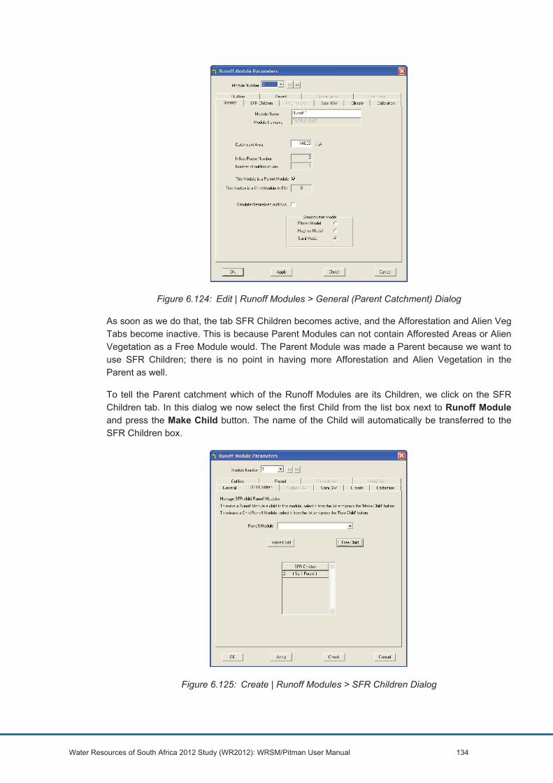
Water Resources of South Africa 2012 Study (WR2012): WRSM/Pitman User Manual 134
Figure 6.124: Edit | Runoff Modules > General (Parent Catchment) Dialog
As soon as we do that, the tab SFR Children becomes active, and the Afforestation and Alien Veg Tabs become inactive. This is because Parent Modules can not contain Afforested Areas or Alien Vegetation as a Free Module would. The Parent Module was made a Parent because we want to use SFR Children; there is no point in having more Afforestation and Alien Vegetation in the Parent as well.
To tell the Parent catchment which of the Runoff Modules are its Children, we click on the SFR Children tab. In this dialog we now select the first Child from the list box next to Runoff Module and press the Make Child button. The name of the Child will automatically be transferred to the SFR Children box.
Figure 6.125: Create | Runoff Modules > SFR Children Dialog

Water Resources of South Africa 2012 Study (WR2012): WRSM/Pitman User Manual 135
Now we do the same for the second Child SL2 – Cane. Should you make a mistake, the Child can be freed by once again selecting it from the list box and then pressing the 'Free Child' button.
If you attempt to add the same Child twice, or try to add a Runoff Module that does not fulfil the criteria for a Child (e.g. the Runoff Module is a Parent, a Child that was already assigned to another Parent or one that has too many outflow routes, or has outflow routes that do not end in Zero Modules) you will be told that this is an illegal operation.
Once we have all the Children in the SFR Child list, we can close the dialog.
Were we to look at the Edit | Runoff Modules > General dialog of SL2 – Forest, we would see:
Figure 6.126: Edit | Runoff Modules > General (SL2 – Forest) dialog
This indicates that Module 13, SL1 – Forest is now a Child to Runoff Module 1.
Note, that the module can now no longer be made a Parent Module, that you cannot run this module for Naturalised Flows anymore and also that we still have the Pitman model as the Groundwater Model. This last point may disconcert you, but it is no reason to be alarmed – the Network has not run, yet, and so the Child does not know any better. Once the simulation runs, the Parent will start to influence it.
The reason for the changes not taking effect immediately is that you could still make all sorts of changes to the Parent Module at this point, and if the changes took effect immediately this could lead to dozens of check messages that all say essentially the same thing when one error message would suffice.
You may also notice that the Paved areas Tab is now inactive. This is because Child catchments may not have paved areas. If there are Paved areas in the catchment, these should be in the Parent catchment. In the same vein, Child catchments may not contain Mining Modules and may not contain WQT, WQT-SAPWAT or WQT Type 4 irrigation blocks.
It is now time to define the afforestation in “SL1 – Forest” and “SL2 – Cane”.
To do this we select the dialog Edit | Runoff Modules > Forest for SL1 – Forest.

Water Resources of South Africa 2012 Study (WR2012): WRSM/Pitman User Manual 136
Figure 6.127: Edit | Runoff Modules > Afforestation (SL1 – Forest) Dialog
You will, no doubt, notice that you have more afforestation options in a Child Module than in a Free module. In addition to Van der Zel and CSIR, you now have two additional choices: Smoothed Gush/Pitman and User defined. A Third option (LUT Gush) will only come into operation once we have created the interface to the Gush database.
First of all, we enter the afforested area. After that, we specify the Smoothed Gush/Pitman option, since that option is new to WRSM/Pitman and we will use the User Defined option in the Child “SL2 – Cane”.
The areas that you enter here will be checked against the area for the entire Child catchment that was entered in the General dialog. Therefore, if we decided not to follow the advice and made the largest possible area there larger than the 30 km² that we know the afforested area to be at maximum extent, this check will not be carried out properly. In that case, if we happen to make a mistake with the areas here, it will not be caught.

Water Resources of South Africa 2012 Study (WR2012): WRSM/Pitman User Manual 137
Figure 6.128: Edit | Runoff Module > Afforestation – Smoothed Gush/Pitman
The Smoothed Gush/Pitman option only requires the percentages of the area that is covered by the three main tree types. Once this is completed, we save this data and turn to the “SL2 – Cane Child”.
Figure 6.129: Edit | Runoff Modules > Afforestation – User Defined
Here we use the User Defined reductions. When we specify the User Defined option, the fields “Required MAR reduction” and “Required Low Flow Reduction” are activated. You can enter your percentage reduction there, and the program will do its best to produce these reductions for you. (This does not mean that all possible combinations of reductions are feasible, of course.)
The required MAR and Low Flow Reduction (in the WRSM/Pitman screen for User Defined) can be obtained from Gush Tables. Note, however, that the Gush Table gives runoffs in mm for both natural and afforested areas, so this information must be converted to percentage reductions. Note also that Gush defines low flow as the average flow for the driest 3 months. This is

Water Resources of South Africa 2012 Study (WR2012): WRSM/Pitman User Manual 138
equivalent to the average of the 25% lowest monthly flows. The computer does this calculation by ranking all monthly flows, selecting the 25% lowest and calculating the mean of this set.
Once the simulation has run and you look at the General dialog of your Child Modules, you will see that they both now use the Sami Groundwater Model, just like the Parent Module. Change the Groundwater model in the Parent and the Groundwater model in the Children will follows suit.
The same goes for the calibration parameters that are used in the Parent. If you change any of them in the Parent Module, they will also be changed in the Child.
There are notable exceptions, though: the values for SL, ST and PI in the Children will be different from those in the Parent. This is because these parameters are adjusted to achieve the reduced flows. The value for FF will also always be 1.00 in Parent Modules, but may be larger than 1.00 in the Children. If you are using the Sami or Hughes Groundwater Models, the value for HGSL will also be different in Children than they were in the Parent.
The outflows in the Route(s) from the Parent Module will be the flows that are generated by the Parent Module itself AND the outflows of the Child Modules.
Should you be interested in the flows that emerged from your Child Module: these flows are saved as usual in the outflow routes that you specified.
And a last tip: It will not help to adjust the calibration parameter values in a Child Module in order to get a better fit between simulated and observed. As soon as the Network Runs, the Parent will overwrite all the Climate data and the Simulation Parameters of the Children with the values that it (the Parent) has.
Obtaining alien vegetation and afforestation requirement time series datafiles (for example as input to the WRYM model)
The outflow route from a child module cannot be taken as representative of what flow is required for either alien vegetation or afforestation. The following method should be used:
To get a time series of alien vegetation flow reductions we need to subtract the flow in the route from the parent runoff module (with child attached) from the flow in the same route but for the naturalised case (i.e. with the naturalised flow tickbox ticked). If a parent runoff module has two child modules, one for afforestation and one for alien vegetation, then one must be removed as a child and the flow in the parent determined and then vice versa. For WRYM input we would also need to run model with alien vegetation (or afforestation) set equal to the present day area for the whole simulation period. To summarise the following procedure would be follows:
• Free say the afforestation child module, change the areas of alien veg so that the start year and end year are for the current area and run. Save the outflow route from the parent. (1)
• Now replace the afforestation as a child module and free the alien vegetation child module. Change the areas of afforestation so that the start year and end year are for the current area and run. Save the outflow route from the parent. (2)
• Now tick the naturalized tickbox in the runoff parent module and run and save the outflow route. (3)
• (3) minus (1) will be the effect of alien vegetation and (3) minus (2) will be the effect of afforestation for use in the WRYM model.

Water Resources of South Africa 2012 Study (WR2012): WRSM/Pitman User Manual 139
Note: If the user wanted to obtain the runoff in the afforested area or area with alien vegetation, the outflow route from the child module could be used but that does not represent the reduction in flow due to afforestation or alien vegetation.
Two examples follow (the first for the Gush/Pitman method and the second for the User Defined option) to illustrate how one should consider the flow balance:
Example 1: Gush/Pitman method – Assume one has an alien vegetation area growing from 0 in 1920 to 177 km² in 2004, that the area of the parent module is 459 km² and that the flow in the parent module is 5.86 * 10 6 m³/a for the situation with the child alien vegetation and 7.03 for the naturalised case. So we can take an average area of 177/2, i.e. 88.5 km². The natural unit MAR for the catchment is 7.03 * 1000 / 459, i.e. 15.32 mm. So, the MAR (as a volume) for the child is 15.32 * 88.5 / 1000, i.e. 1.356 * 10 6 m³/a. This agrees with the value for virgin MAR in the “WRSM2000.ERR” datafile of 1.357 * 10 6 m³/a.
The “WRSM2000.ERR” datafile gives a target MAR of 0.569 * 10 6 m³/a (about 48%), but achieved a final MAR of 0.529 * 10 6 m³/a, as against the final MAR in the outflow route of the child module of 0.16, BUT we have a riparian area of 2.2% which can easily account for the extra 0.37 reduction. (Without any riparian % one gets a flow in the child outflow route of 0.52 * 10 6 m³/a ).
The difference in MAR between the naturalised and non-naturalised analyses is 7.03-5.86, i.e. 1.17 * 10 6 m³/a, which represents the reduction due to alien vegetation. If we add the 0.16 to this we should get the natural MAR of the child, i.e. 1.33 * 10 6 m³/a. This is not too far off the natural MAR in the “WRSM2000.ERR” datafile of 1.357.
Example 2: User Defined Method – Assume a child module with area of 103.1 km² out of a total catchment area of 244 km² with user defined % reduction in MAR of 62.95% .The afforested area therefore represents 42.3% of the total area. The natural MAR for the total catchment is 24.5 * 10 6
m³/a so the expected MAR for the child outflow route is 24.5 * 103.1/244 = 10.35 * 10 6 m³/a for the child module in its natural state. The simulated MAR for the child outflow route is 3.8 * 10 6 m³/a which means a reduction of 10.35 – 3.8 = 6.55 which represents 63% of the natural MAR which agrees well with the user defined target reduction of 62.95%. The reason why an exact agreement will not always be reached is due to the iteration procedure – the model tries to get within 1% of the target flow reduction but if this is not reached within 10 iterations, it increases the closing error until closure is achieved (40 iterations allowed in total).
Summary and additional notes
Every one of the SFR-catchments (Child modules) is a Runoff Module in its own right. A Child Module must have at least an area, one (1) outflow route and climate data. The area of a Child Module should be the maximum area that will be covered by the forest/alien vegetation/user defined vegetation during the simulation period. The area of the Child Module serves as a check to make sure that the forest, etc. does not accidentally grow beyond its maximum area.
When it is created, a Child Module does not have to have all the data that it would need to run independently. Once it has been simulated once, it will have 'inherited' all of the parameters from the Parent Module in which it lies.
A Parent Module is just another Runoff Module in which the Child(ren) reside. The Parent Module has an area that encompasses all of the Children and the areas between them.

Water Resources of South Africa 2012 Study (WR2012): WRSM/Pitman User Manual 140
Parent and Child Modules can be created in any order, however not all SFR algorithms are available to 'Free' Modules and they must be made Children before these algorithms can be accessed.
Any Free Runoff Module that fulfils the criteria can be added to a Parent Module. Such Modules may only have one outflow Route and this route must lead to a Zero Sink Module. They may also not contain Mining or Irrigation modules or Paved areas.
Once a Free Module is added to a group governed by a Parent, it becomes a Child. This gives the Module access to additional SFR algorithms. If the climate data or one or more parameters are changed in the Parent, these parameters are passed down to the Child Modules. Some of the simulation parameters will be adjusted by means of the reduction algorithms or curves, others will be passed down as they are.
Any Child Module can be taken out of the group of Child modules that are governed by a Parent at any time. In the same vein, other sub-catchments can be added to a Parent once they are created. If a Child is no longer governed by a Parent (but was not taken out of the network), it will run as a 'Free' runoff module, but since the outflow is routed to a Zero sink Module, the flows will not be taken into account
When the simulation runs, the Parent Module governs when the Child Modules are calculated. When a Parent Module is run, it first instructs all of its Child Modules to run their simulation. The position of the Child Module in the Network is therefore immaterial, and only the position of a Parent Module needs to be changed in the event of a Sequence error.
Active area. During simulation, the active area of a Child Module is only that area that is afforested, covered with Alien Vegetation, under sugar cane, etc. as specified by means of the year/area pairs in the Child Module. Only the outflows from that area are reduced using the algorithm that is specified for that Child Module. The portion of the Child catchment that is not afforested (etc.) in the given month is ignored – it is 'given' to the Parent catchment.
When the Parent catchment is simulated, its area is reduced by the active Child areas of every one of the Child-catchment for every specific month (since the areas under vegetation can grow or shrink).
Once the simulation is complete, we add the outflows from the SFR Child catchments to the flows from the Parent catchment, and that is the final outflow of the catchment.
Groundwater Storage States are stored as a Module time series for each Child Module as they were calculated.
The Groundwater Storage State in the Parent Module is an Area-weighted average of all the Groundwater Storage States – in the Parent and in the Child areas.
A Parent may have many children, but a Child may have only one Parent.
A Parent catchment may not have afforested or alien vegetation areas other than in its children, unless it has a calibration parameter FT = 0 in which case it must not be a Parent and can then have afforestation and/or alien vegetation.
A Parent catchment may have paved areas.
A Child catchment may not contain paved areas.
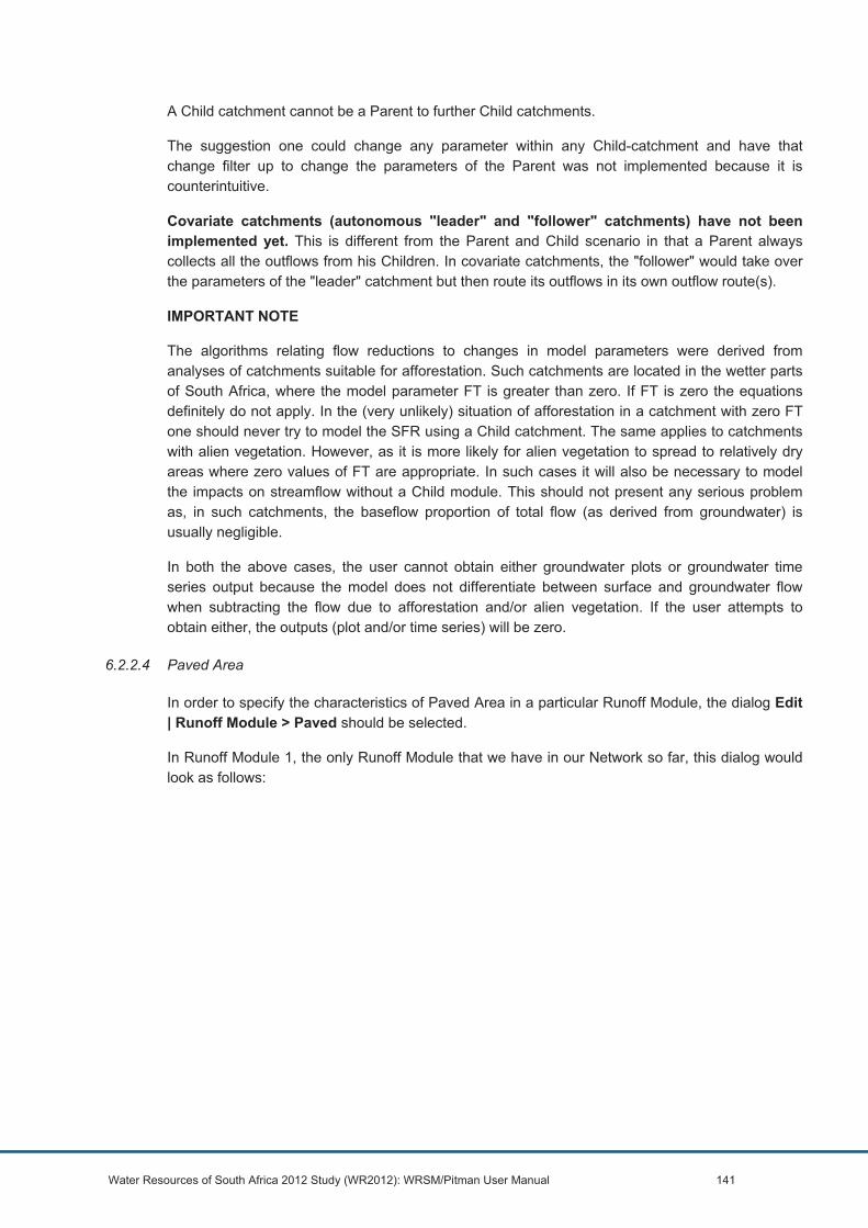
Water Resources of South Africa 2012 Study (WR2012): WRSM/Pitman User Manual 141
A Child catchment cannot be a Parent to further Child catchments.
The suggestion one could change any parameter within any Child-catchment and have that change filter up to change the parameters of the Parent was not implemented because it is counterintuitive.
Covariate catchments (autonomous "leader" and "follower" catchments) have not been implemented yet. This is different from the Parent and Child scenario in that a Parent always collects all the outflows from his Children. In covariate catchments, the "follower" would take over the parameters of the "leader" catchment but then route its outflows in its own outflow route(s).
IMPORTANT NOTE
The algorithms relating flow reductions to changes in model parameters were derived from analyses of catchments suitable for afforestation. Such catchments are located in the wetter parts of South Africa, where the model parameter FT is greater than zero. If FT is zero the equations definitely do not apply. In the (very unlikely) situation of afforestation in a catchment with zero FT one should never try to model the SFR using a Child catchment. The same applies to catchments with alien vegetation. However, as it is more likely for alien vegetation to spread to relatively dry areas where zero values of FT are appropriate. In such cases it will also be necessary to model the impacts on streamflow without a Child module. This should not present any serious problem as, in such catchments, the baseflow proportion of total flow (as derived from groundwater) is usually negligible.
In both the above cases, the user cannot obtain either groundwater plots or groundwater time series output because the model does not differentiate between surface and groundwater flow when subtracting the flow due to afforestation and/or alien vegetation. If the user attempts to obtain either, the outputs (plot and/or time series) will be zero.
6.2.2.4 Paved Area
In order to specify the characteristics of Paved Area in a particular Runoff Module, the dialog Edit | Runoff Module > Paved should be selected.
In Runoff Module 1, the only Runoff Module that we have in our Network so far, this dialog would look as follows:

Water Resources of South Africa 2012 Study (WR2012): WRSM/Pitman User Manual 142
Figure 6.130: The Edit | Runoff Modules > Paved dialog
The Paved Area algorithm only comes into effect when Year/Area data is entered into the module.
To add Paved Area year/area pairs, enter the values in the edit mask and press the Add button. To edit a pair, either enter the data for the same year again and press the Add button or you can click on either the year or the area value of the year/area pair in the list that you want to change. When you click on a pair, the values will be transferred to the edit mask. Once you have changed the values, you can store them back in the list by pressing the Add button. To delete a pair, click on one of the values of the pair to delete in the list, and press the Delete button.
The Paved Area year/area data must cover the entire simulation period. If this is not the case, the module will issue a warning. The Paved Area is determined for every given year in the simulation. Unless the data starts on or before the first year in the simulation period, and ends on or after the last year of simulation, the interpolation routine would break down.
The Paved area can never be greater than the total area of the catchment. The total area covered by Afforestation, Alien Vegetation and Paved area may also not exceed the total area of the catchment.
Note: If one takes the outflow from a runoff module with paved areas and subtracts the naturalised flows, one would expect only positive flow differences. However there are normally relatively small negatives especially in the winter months. The reason is that with paved areas the soil moisture (Pitman S) is lower than without, because they prevent some of the rain infiltrating. So, in the dry season (when there is little or no runoff from the paved areas), the interflow/groundwater flow is higher without paved areas and so is the total flow. There can also be a negative difference in a month with relatively high rainfall where the "unpaved" Pitman S is higher at start of the month, so it will reach saturation sooner than the paved case. Once saturation is reached, all the excess rainfall becomes runoff so the unpaved case generates more runoff than the paved case.
6.2.3 Special Features, Areas and Routes in the Channel Module.
There are four special features in the Channel Module, namely:
• bedlosses;

Water Resources of South Africa 2012 Study (WR2012): WRSM/Pitman User Manual 143
• the Basic Wetlands Model; • the Comprehensive Wetlands Model and • the Diversion Route.
Within the Comprehensive Wetlands Model, there are two further features: the local inflow route and the local outflow route.
To choose one of the special features, open the Edit | Channel Modules > General dialog and select the Module that you wish to edit:
Figure 6.131: The Edit | Channel Modules > General dialog
To choose a Special feature, click on the radio button of the feature that you want and press the Apply button. Nothing will happen until you press the Apply button, because it is possible to swap between the different Special Features. When you do this, some of the data that you entered for (for example) a Comprehensive Wetlands may not have been saved.
Although you can swap between the different Special Features and the data for the different features will be preserved, only one of them will be effective (i.e. simulated) at any given time in a given Module. The only exception to this is Bedlosses which may be specified for the Channel regardless of whether a special feature is chosen from the list or not.
Note that if you choose the Basic Wetlands, the dialogs Diversion and Wetlands (C) (for Comprehensive) will be deactivated and the dialog Wetlands (B) (for Basic) will be active. As soon as you enter either bedloss, wetlands or diversion Route data, the tick box next to Module has special feature data will be ticked. This tick mark is read-only and has no function other than to remind you that this Module has Special Feature Data – it is useful when you scroll through your Channel Modules.
To model any form of Wetlands, the Module will require information about the climate. If this data is not supplied, the program will issue an error message and the Module will be invalid. The

Water Resources of South Africa 2012 Study (WR2012): WRSM/Pitman User Manual 144
Climate dialog is similar to that in the other modules, and can be reached by means of the Edit | Channel Modules > Climate dialog:
Figure 6.132: The Edit | Channel Modules > Climate dialog
6.2.3.1 Bedlosses
In its simplest form, a Channel Module consists of one inflow route and a single outflow route and has no special features. In this state, the Channel Module can only be used to simulate bedlosses.
To simulate Bedlosses in a specific module, we select the dialog Edit | Channel Modules > Bedloss. This dialog has only one field labelled Bedloss where the flow that is lost (in million m³ per month) can be entered.
The algorithm that simulates the bedlosses in the Channel Module is very simple. If enough flow enters the Channel Module via the inflow route(s) in a given month, the bedlosses will be subtracted from the inflows and the resulting flow is routed to the outflow route. If the flow is less than the bedloss, the resultant outflow will be zero.
In the case where a Channel Model has defined and/or calculated outflow routes in addition to the primary outflow route, the bedlosses will be subtracted from the sum total inflow first. If the Channel Module has defined outflow routes, then these demands from these routes are satisfied after the bedlosses are served. It is only after these demands are satisfied that the calculated demands (such as those calculated from Irrigation Modules) are serviced.
Where any of the Special Features (Wetlands or Diversion Routes) are specified for the Module, these are calculated after the bedlosses have been subtracted.
Important: The bedlosses that are subtracted from the inflow are lost to the system. They do not become part of the groundwater system and do not re-enter the network anywhere else.

Water Resources of South Africa 2012 Study (WR2012): WRSM/Pitman User Manual 145
6.2.3.2 The Basic Wetlands Model
The Basic Wetlands Model is the Wetlands Model that was available in WRSM90 and in WRSM/Pitman prior to version 2.25xx. If you load a Network with a wetland in a Channel Module that was produced with an earlier version of the program, this is the Model that will be used.
The parameters of the Basic Wetlands Model are entered in the dialog Edit | Channel Modules > Wetlands (B). This dialog looks as follows:
Figure 6.133:The Edit | Channel Modules > Wetlands(B) dialog
Only three parameters are required for the Basic Wetlands Model, the Wetland Area, the Wetland storage and the Recharge coefficient, which is usually equal to 1.0 unless one is attempting to model the impact of an aquifer.
6.2.3.3 The Comprehensive Wetlands Model
The comprehensive Wetlands model is described in detail in WRSM/Pitman Theory (Stewart Scott, 2006).
In order to specify the Comprehensive Wetlands Model in a Channel Module, choose the radio button Comprehensive Wetlands in the dialog Edit | Channel Modules > General dialog for the Module with the appropriate Module Number. Once you press the Apply button in that dialog, the dialog Wetlands (C) will become active and can be chosen.
The dialog Edit | Channel Modules > Wetlands (C) will look as follows:

Water Resources of South Africa 2012 Study (WR2012): WRSM/Pitman User Manual 146
Figure 6.134: The Edit | Channel Modules > Wetlands(C) dialog
In this dialog, you can choose a Local Wetlands Inflow Route. A local wetlands inflow route is NOT the river channel that routes water from the river channel into the wetlands – it is an inflow directly into the wetlands from outside of the Channel Module.
A local wetlands inflow route can be any of the inflow routes that you have defined for the Channel Module. If you want to add an inflow route but there are no Inflow routes in the menu when you click on the arrow to the right of the field, you probably have not added any inflow routes to the Channel Module, and you should do that first.
The same applies to the Local Wetlands Outflow / Abstraction Route. This route is NOT the return flow from the Wetlands back into the river channel, but it is an abstraction from the wetland to somewhere external to the Channel Module. It is important to appreciate that the primary outflow route to the Channel Module cannot be a local outflow route, because the primary outflow route must transport the final outflows of the Channel Module. Under normal circumstances, the Local Wetlands Outflow route would carry defined flows but it could also be the Abstraction Route of an Irrigation Module.
If a Local Wetlands Inflow Route has defined flows, the name of the file will appear in the field labelled Inflows file. This is a read-only field and you cannot change the name of the file by changing this field. To change the flows file for the route, you should call up the dialog Edit | Routes > Defined flows.
The same applies to the field labelled Outflows file. It is also read-only and the file name can also only be changed in the Edit | Routes > Defined flows dialog.
The other parameters, the Area of the Wetlands, the Volume of Wetlands, the Power of the Volume/area curve, the Bankfull capacity of the river channel (million m³/month) and the proportion of the in- and outflow of the wetlands area are described in detail in (Stewart Scott, 2006).

Water Resources of South Africa 2012 Study (WR2012): WRSM/Pitman User Manual 147
6.2.3.4 The Diversion Route
A diversion route, as its name implies, diverts flows from the Channel Module into a specified route. Diversion routes are only active if the 'Diversion Route' Radio Button in the 'Special Features' group in the Edit | Channel Modules > General dialog is activated.
In a new Channel Module, the 'Special Features' will be set to 'None' and the tabs for 'Wetlands (B)', 'Wetlands C' and 'Diversion' in the dialog will be disabled.
Once the 'Special Feature' 'Diversion Route' is clicked and the radio button is on (black), one should press the 'Apply' button to tell the dialog that this is what one wants. When the apply button is pressed, the Tab marked 'Diversion' will be activated.
Clicking on the Diversion tab will open the dialog for the diversion route.
Figure 6.135: The Edit | Channel Modules > Diversion dialog
In the field labelled Diversion Outflow Route you can choose the route that is to carry the diverted flows. If there are no routes in the diversion routes menu, this probably means that you have not added any outflow routes to your Channel Reach Module, and you should do that first.
A diversion route can be any outflow route from the Channel Module except the primary outflow route. Diversion routes can be used in all possible configurations – it can be connected to a downstream module, a zero module, a channel reach, an irrigation block or a reservoir and may be given defined demands in the form of a flows file. The way that these are handled is described below.
The bankfull level limits the abstraction into the Diversion to 0 when the flow in the Channel Module is less than the specified level. It means "Flow in river above which abstraction/diversion can take place". This could be due to downstream requirements for ecological or other purposes and/or physical constraints on the abstraction/diversion works.
Diversion efficiency relates to the efficiency with which water can be abstracted/diverted into the Diversion Route.

Water Resources of South Africa 2012 Study (WR2012): WRSM/Pitman User Manual 148
The Maximum monthly diversion capacity limits the flow that can be abstracted in a given month.
Available flow as used below is the flow over bankfull level multiplied by the diversion efficiency. The maximum flow that is diverted in a given month is therefore the minimum of the available flow and the diversion capacity.
qinw = AMIN1(qdivcap, drprqin * (qtot – drqbnk))
Where “qtot” is the total flow in the Channel Module AFTER discounting all bedlosses and defined and calculated abstractions that were made by the 'normal' abstraction routes to this Channel Module.
There are however a few extra rules that had to be implemented to make sure that the diversion route would function as expected – mainly depending on the module that is attached downstream of this route and what a user is allowed (and likely) to do with the diversion route itself.
Diversion to a Zero Module
(a) No defined flows
When the Diversion Route option is active and the flows higher than the specified bankfull level, flows up to the maximum capacity are diverted into the Diversion Route. The supply is therefore the minimum of available and the maximum capacity.
If the Diversion Route option is not active (i.e. Special Feature is 'None' or one of the Wetlands) no diversions will be made to the Diversion Route.
(b) With defined flows from a file
When the Diversion Route option is active and the flows higher than the specified bankfull level, flows up to the maximum capacity are diverted into the Diversion Route if the defined flows (which act as demand) specify that this much should be diverted. The supply is therefore the minimum between what is available, what is demanded and the maximum capacity.
If the Diversion Route option is not active (i.e. Special Feature is either 'None' or one of the Wetlands) the route with a defined flows file acts as a normal outflow file with a defined flow. The supply is the minimum between what is available in the Channel Reach and the Demand.
Diversion to another Channel Module
The same rules apply as in the case of Diversion to a Zero Module.
Diversion to an Irrigation Module
Here the Irrigation Module sets the demands and diversions are only made up to the maximum demanded by the irrigation block. The supply is therefore the minimum between what is available, what is demanded and the maximum route capacity.
If the Diversion Route option is not active (i.e. Special Feature is either 'None' or one of the Wetlands) the Irrigation Module abstraction route acts as a normal Irrigation abstraction route.

Water Resources of South Africa 2012 Study (WR2012): WRSM/Pitman User Manual 149
The supply is the minimum between what is available in the Channel Module and the Demand. If there is a deficit, the Irrigation abstractions are reduced proportionally together with the flows in the other calculated routes.
In both cases, when the supply is less than the demand, the Irrigation Module is told to adjust the supply to what is supplied in the route.
Diversion to a Reservoir
When the Diversion Route option is active and the flows higher than the specified bankfull level, the Diversion Module asks the Reservoir for the spare capacity that it has. This spare capacity becomes the demand on the route. When a Reservoir is full, the spare capacity will be 0 and therefore the demand will be 0.
With the current configuration, a Reservoir can only be solved once all of the inflows and demands on it are known or defined. This means that we can only ask the reservoir to supply the spare capacity for the end of the previous month, since the reservoir itself has not been solved for the month in which we need the data, because it has to wait until it has that data.
The result is that a Reservoir that is fed by means of a Diversion Route will sometimes spill – especially in months of high rainfall. This will be made worse still if the reservoir has inflows of its own that are fed by a catchment.
The spillages from the Reservoir can, of course, be routed to a downstream Channel Module again, but the flows that are reported by the diversion route will be higher than would be strictly necessary. This should be borne in mind, especially when simulating an active pumping situation.
If the Diversion Route option is not active (i.e. Special Feature is either 'None' or one of the Wetlands) the route operates under the same rules as those for a Zero Module. Flows would only enter this route if it has would require a defined flows file, or no flows would be send down the route.
6.2.4 Special Features in the Reservoir Module
The Reservoir Module has two special features, namely:
• The Monthly Defined Abstraction and • Water Restrictions
These two features are related in that water restrictions can only be implemented on a route where monthly defined abstractions were specified.
6.2.4.1 Defining a Route with Monthly Defined Abstractions
To define a route from a reservoir with monthly defined abstractions, we use the menu point File | Add New | Route. This will produce the following dialog:

Water Resources of South Africa 2012 Study (WR2012): WRSM/Pitman User Manual 150
Figure 6.136: The New Route dialog
We adopt the proposed route number and make the Route originate in Reservoir RV7 and flow towards a Zero Sink Module. When we press the OK button, the following dialog will pop up:
Figure 6.137: The Route parameter dialog
This is the dialog that can also be called up by means of the menu point Edit | Routes > Defined Flows. By entering the twelve monthly defined abstractions, the route is a monthly defined abstractions route.
It is possible to redefine an existing Reservoir outflow route from a defined flows file flow to a defined monthly abstractions flow by means of the Edit | Routes > Defined Flows menu point. In this case, if you have defined this route before with a flows file, the name of the Flows file will be in the field labelled Flows File. At this point, the mask to enter the 12 monthly abstractions will be greyed out. Should you wish to redefine such a route to a Defined monthly abstractions route, first delete the name of the file in the Flows File field. Once the Flows File field is empty and you press the Apply button, both the “Flows File” field and the “Defined monthly abstractions” fields will be active. Once you have entered data in either of these two fields and you have pressed the Apply button, the field that was not used will be deactivated to stop you from accidentally entering conflicting data.
Please note that flow files must cover the full record period, i.e. enter zeroes for the months and years where the data is not applicable.
6.2.4.2 Setting the Water restrictions on a Route with Monthly Defined Abstractions
To set the Water Restrictions on a Reservoir Outflow Route with monthly defined abstractions, we use the menu point Edit | Reservoir > Restrictions. This dialog will look as follows:
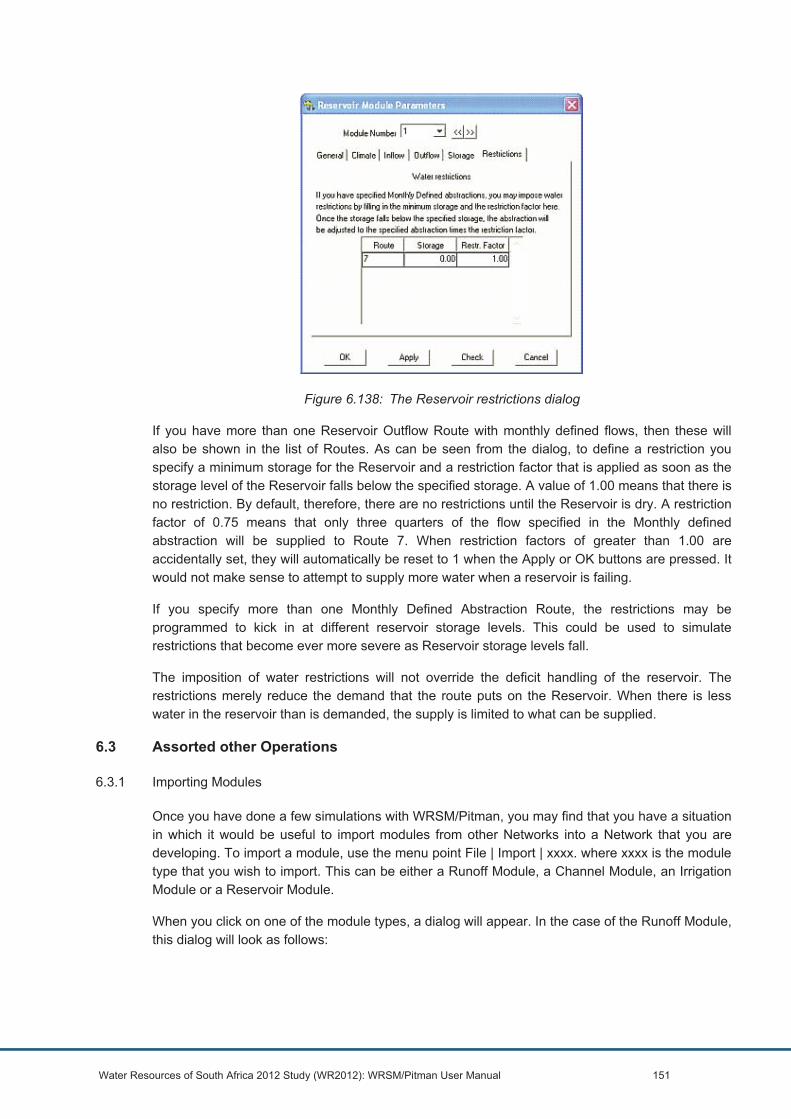
Water Resources of South Africa 2012 Study (WR2012): WRSM/Pitman User Manual 151
Figure 6.138: The Reservoir restrictions dialog
If you have more than one Reservoir Outflow Route with monthly defined flows, then these will also be shown in the list of Routes. As can be seen from the dialog, to define a restriction you specify a minimum storage for the Reservoir and a restriction factor that is applied as soon as the storage level of the Reservoir falls below the specified storage. A value of 1.00 means that there is no restriction. By default, therefore, there are no restrictions until the Reservoir is dry. A restriction factor of 0.75 means that only three quarters of the flow specified in the Monthly defined abstraction will be supplied to Route 7. When restriction factors of greater than 1.00 are accidentally set, they will automatically be reset to 1 when the Apply or OK buttons are pressed. It would not make sense to attempt to supply more water when a reservoir is failing.
If you specify more than one Monthly Defined Abstraction Route, the restrictions may be programmed to kick in at different reservoir storage levels. This could be used to simulate restrictions that become ever more severe as Reservoir storage levels fall.
The imposition of water restrictions will not override the deficit handling of the reservoir. The restrictions merely reduce the demand that the route puts on the Reservoir. When there is less water in the reservoir than is demanded, the supply is limited to what can be supplied.
6.3 Assorted other Operations
6.3.1 Importing Modules
Once you have done a few simulations with WRSM/Pitman, you may find that you have a situation in which it would be useful to import modules from other Networks into a Network that you are developing. To import a module, use the menu point File | Import | xxxx. where xxxx is the module type that you wish to import. This can be either a Runoff Module, a Channel Module, an Irrigation Module or a Reservoir Module.
When you click on one of the module types, a dialog will appear. In the case of the Runoff Module, this dialog will look as follows:
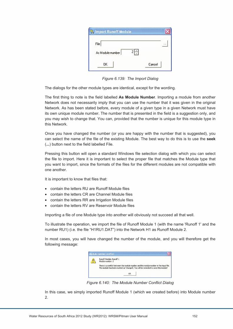
Water Resources of South Africa 2012 Study (WR2012): WRSM/Pitman User Manual 152
Figure 6.139: The Import Dialog
The dialogs for the other module types are identical, except for the wording.
The first thing to note is the field labelled As Module Number. Importing a module from another Network does not necessarily imply that you can use the number that it was given in the original Network. As has been stated before, every module of a given type in a given Network must have its own unique module number. The number that is presented in the field is a suggestion only, and you may wish to change that. You can, provided that the number is unique for this module type in this Network.
Once you have changed the number (or you are happy with the number that is suggested), you can select the name of the file of the existing Module. The best way to do this is to use the seek (...) button next to the field labelled File.
Pressing this button will open a standard Windows file selection dialog with which you can select the file to import. Here it is important to select the proper file that matches the Module type that you want to import, since the formats of the files for the different modules are not compatible with one another.
It is important to know that files that:
• contain the letters RU are Runoff Module files • contain the letters CR are Channel Module files • contain the letters RR are Irrigation Module files • contain the letters RV are Reservoir Module files
Importing a file of one Module type into another will obviously not succeed all that well.
To illustrate the operation, we import the file of Runoff Module 1 (with the name 'Runoff 1' and the number RU1) (i.e. the file “H1RU1.DAT”) into the Network H1 as Runoff Module 2.
In most cases, you will have changed the number of the module, and you will therefore get the following message:
Figure 6.140: The Module Number Conflict Dialog
In this case, we simply imported Runoff Module 1 (which we created before) into Module number 2.

Water Resources of South Africa 2012 Study (WR2012): WRSM/Pitman User Manual 153
This message simply warns you that the Module number in the file was different from what the program expected, and that it will insist on saving the module to the input directory of the Network once you save the Network, Close it or when you Exit the program.
In most cases, the program will find quite a few conflicts between the data in the data file and what is possible in the current Network. So, for example, it will tell you that certain Route numbers that are specified in the data file can not be used twice in a Network and so on. These error messages do not mean that the operation failed, but that your intervention is required to resolve conflicts between the existing Routes and Modules and the new Module.
Eventually, you will get the message:
Figure 6.141: The import module, input file error
Usually the errors are not half as dramatic as they seem at first and a little checking – especially where it concerns the in- and outflow routes of the new Module – will soon put things right.
Note that gauging stations cannot be imported, mainly because the chances that a route will have the same source and sink modules and have the same route number in two different Networks are not very good. Routes, too, are never imported but created anew when they are needed.
6.3.2 Deleting Modules
From time to time is may be necessary to delete a module from a Network. This, too, can be done from within WRSM/Pitman.
The menu point to use to delete a module is the menu point File | Delete | xxxx where xxxx can be Runoff Module, Channel Module, Irrigation Module or Reservoir Module. To delete Runoff Module 2 which we created above, for example, we use menu point File | Delete | Runoff Module. This will show the following dialog:
Figure 6.142: The Delete Module Dialog
To select a Module, you can click on the down arrow to the right of the input field. This will open a drop-down menu in which all the Runoff Modules are listed. Once the number and name of the module to be deleted is in the field, pressing the OK button will delete the Module. Once the
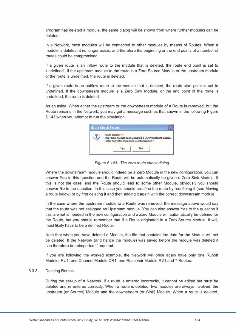
Water Resources of South Africa 2012 Study (WR2012): WRSM/Pitman User Manual 154
program has deleted a module, the same dialog will be shown from where further modules can be deleted.
In a Network, most modules will be connected to other modules by means of Routes. When a module is deleted, it no longer exists, and therefore the beginning or the end points of a number of routes could be compromised.
If a given route is an inflow route to the module that is deleted, the route end point is set to 'undefined'. If the upstream module to the route is a Zero Source Module or the upstream module of the route is undefined, the route is deleted.
If a given route is an outflow route to the module that is deleted, the route start point is set to undefined. If the downstream module is a Zero Sink Module, or the end point of the route is undefined, the route is deleted.
As an aside: When either the upstream or the downstream module of a Route is removed, but the Route remains in the Network, you may get a message such as that shown in the following Figure 6.143 when you attempt to run the simulation.
Figure 6.143: The zero route check dialog
Where the downstream module should indeed be a Zero Module in the new configuration, you can answer Yes to this question and the Route will be automatically be given a Zero Sink Module. If this is not the case, and the Route should lead to some other Module, obviously you should answer No to the question. In this case you should redefine the route by redefining it (see Moving a route below) or by first deleting it and then adding it again with the correct downstream module.
In the case where the upstream module to a Route was removed, the message above would say that the route was not assigned an Upstream module. You can also answer Yes to the question if this is what is needed in the new configuration and a Zero Module will automatically be defined for the Route, but you should remember that if a Route originated in a Zero Source Module, it will, most likely have to be a defined Route.
Note that when you have deleted a Module, the file that contains the data for the Module will not be deleted. If the Network (and hence the module) was saved before the module was deleted it can therefore be reimported if required.
If you are following the worked example, the Network will once again have only one Runoff Module, RU1, one Channel Module CR1, one Reservoir Module RV1 and 7 Routes.
6.3.3 Deleting Routes
During the set-up of a Network, if a route is entered incorrectly, it cannot be edited but must be deleted and re-entered correctly. When a route is deleted, two modules are always involved: the upstream (or Source) Module and the downstream (or Sink) Module. When a route is deleted,
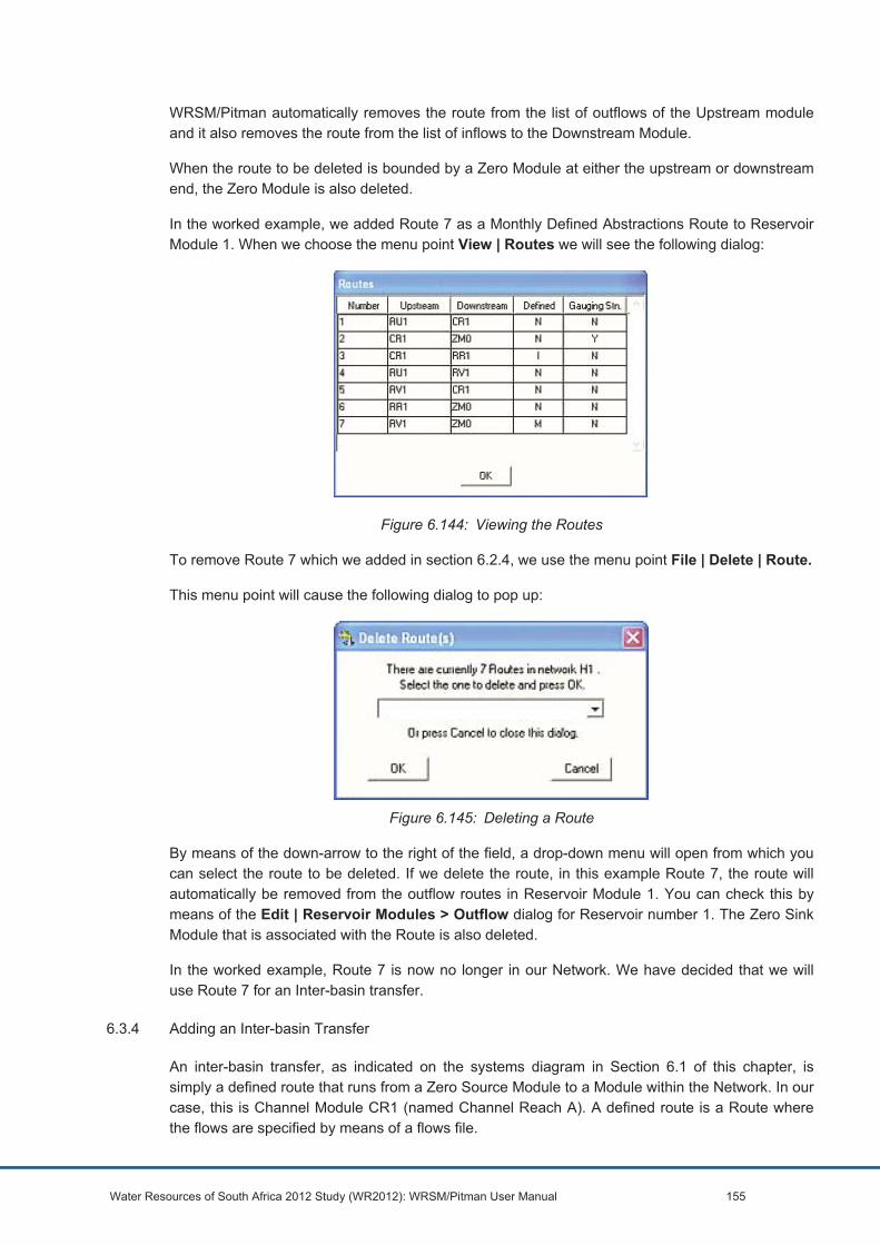
Water Resources of South Africa 2012 Study (WR2012): WRSM/Pitman User Manual 155
WRSM/Pitman automatically removes the route from the list of outflows of the Upstream module and it also removes the route from the list of inflows to the Downstream Module.
When the route to be deleted is bounded by a Zero Module at either the upstream or downstream end, the Zero Module is also deleted.
In the worked example, we added Route 7 as a Monthly Defined Abstractions Route to Reservoir Module 1. When we choose the menu point View | Routes we will see the following dialog:
Figure 6.144: Viewing the Routes
To remove Route 7 which we added in section 6.2.4, we use the menu point File | Delete | Route.
This menu point will cause the following dialog to pop up:
Figure 6.145: Deleting a Route
By means of the down-arrow to the right of the field, a drop-down menu will open from which you can select the route to be deleted. If we delete the route, in this example Route 7, the route will automatically be removed from the outflow routes in Reservoir Module 1. You can check this by means of the Edit | Reservoir Modules > Outflow dialog for Reservoir number 1. The Zero Sink Module that is associated with the Route is also deleted.
In the worked example, Route 7 is now no longer in our Network. We have decided that we will use Route 7 for an Inter-basin transfer.
6.3.4 Adding an Inter-basin Transfer
An inter-basin transfer, as indicated on the systems diagram in Section 6.1 of this chapter, is simply a defined route that runs from a Zero Source Module to a Module within the Network. In our case, this is Channel Module CR1 (named Channel Reach A). A defined route is a Route where the flows are specified by means of a flows file.

Water Resources of South Africa 2012 Study (WR2012): WRSM/Pitman User Manual 156
In the worked example, we have removed the temporary Route 7 from Reservoir 1 in the Network and will now add a route with this number as an Inter-basin Transfer to the Network. To do this, we add the route by means of the menu point File | Add New | Route.
Figure 6.146: Adding a New Route 7
Once we press the OK button, we will get the dialog:
Figure 6.147: Adding a defined flow
(the Edit | Routes > Defined Flows dialog for route 7). We select the appropriate flows file to define the flows by pressing the seek (...) button next to the field labelled Flows File.
When we press the OK button, the inter-basin transfer is ready for use.
6.3.5 Moving a Route
When we decide to add extra modules to an existing Network, some of the end points of the routes that we have created before will have to be moved.
If you have followed the creation of the Network of the worked example so far, you have a network that ends at a Zero Sink Module at the downstream end of Route 2. Route 2 has a Gauging Station GS1 as can be seen from the systems Diagram.
If we now add Channel Module CR3 to the Network, Route 2 will still be connected to its Zero Sink Module. I choose to number the next Channel Module as CR 3 instead of CR 2 to show that you do not have to follow the numbering that is suggested by the program.
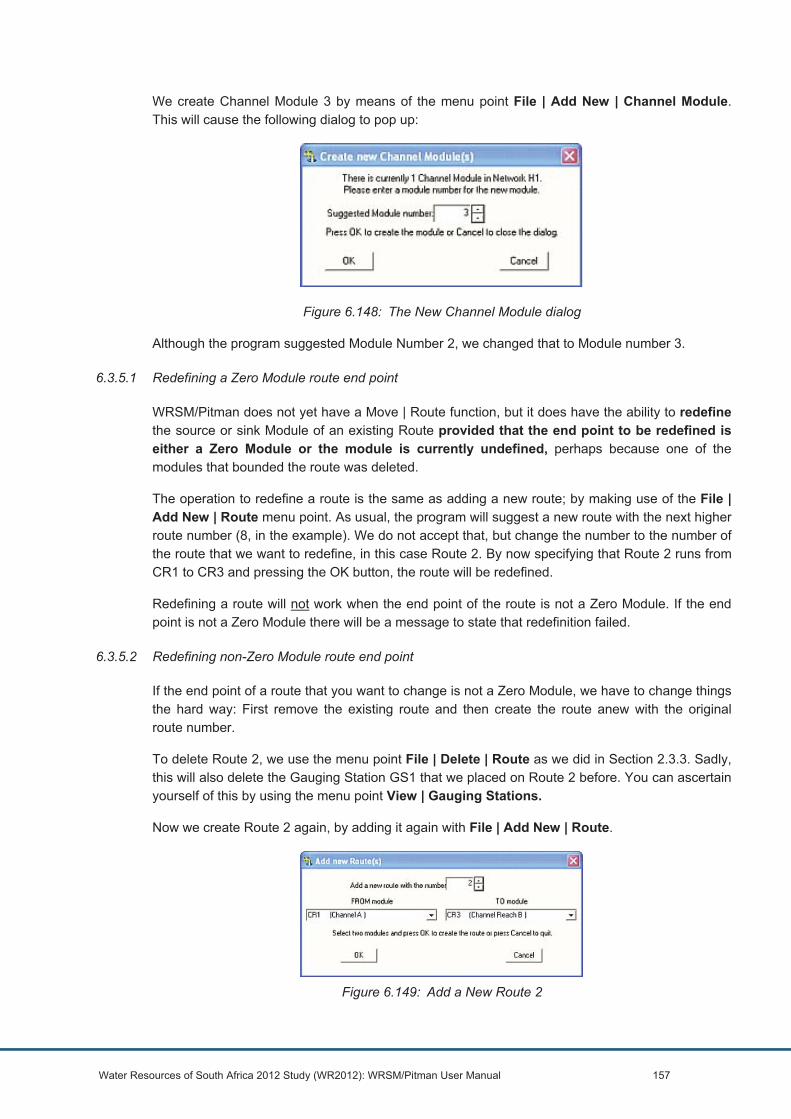
Water Resources of South Africa 2012 Study (WR2012): WRSM/Pitman User Manual 157
We create Channel Module 3 by means of the menu point File | Add New | Channel Module. This will cause the following dialog to pop up:
Figure 6.148: The New Channel Module dialog
Although the program suggested Module Number 2, we changed that to Module number 3.
6.3.5.1 Redefining a Zero Module route end point
WRSM/Pitman does not yet have a Move | Route function, but it does have the ability to redefine the source or sink Module of an existing Route provided that the end point to be redefined is either a Zero Module or the module is currently undefined, perhaps because one of the modules that bounded the route was deleted.
The operation to redefine a route is the same as adding a new route; by making use of the File | Add New | Route menu point. As usual, the program will suggest a new route with the next higher route number (8, in the example). We do not accept that, but change the number to the number of the route that we want to redefine, in this case Route 2. By now specifying that Route 2 runs from CR1 to CR3 and pressing the OK button, the route will be redefined.
Redefining a route will not work when the end point of the route is not a Zero Module. If the end point is not a Zero Module there will be a message to state that redefinition failed.
6.3.5.2 Redefining non-Zero Module route end point
If the end point of a route that you want to change is not a Zero Module, we have to change things the hard way: First remove the existing route and then create the route anew with the original route number.
To delete Route 2, we use the menu point File | Delete | Route as we did in Section 2.3.3. Sadly, this will also delete the Gauging Station GS1 that we placed on Route 2 before. You can ascertain yourself of this by using the menu point View | Gauging Stations.
Now we create Route 2 again, by adding it again with File | Add New | Route.
Figure 6.149: Add a New Route 2

Water Resources of South Africa 2012 Study (WR2012): WRSM/Pitman User Manual 158
The program will suggest that we use the route number 8, but since we know that there is no Route 2 anymore (we have just deleted it) we can reuse that number.
Finally, we Add the Gauging Station to the new Route 2 by using the menu point File | Add New | Gauging Station as we did in Section 6.1.12.
To run the simulation, Channel Module 3 still needs an outflow Route, defined as the primary outflow route (Route 20 in the diagram), but this was already demonstrated in Section 6.1.10
All further operations to complete the Network that was designed in the System Diagram at the beginning of this chapter are simply repetitions of the steps above.
6.3.6 Saving Statistics
To save the statistics of simulated versus observed flows to a file, you can use the menu point Save | Statistics after you have run the simulation. This will create a file with the name “H1All.OUT” in the output folder that you specified for the Network. This file will contain the parameters of all the Runoff Modules in a particular Network and the statistics of observed and simulated flows at all the Gauging Stations. If this file already exists, you will be asked whether you wish another name for this file or whether it can be overwritten.
Note that the statistics are calculated only for flows at Gauging Stations and that the Network must therefore feature at least one Gauging Station. If no gauging stations are present, the statistics are not calculated.
The file can be viewed by means of the menu point View | Any File, from where the file can also be printed.
An alternative method to produce a printout of the statistics is to use the File | Print | Statistics menu option. When you use this menu point the following dialog pops up:
Figure 6.150: The Hardcopy Options
Under normal circumstances, these settings are adequate for the report. It is recommended that the Courier Font is not changed. Courier is a fixed character width font that will ensure that the tables that are produced will be properly spaced. Choosing a different font may produce a printout that is less than pretty to behold.
In Section 6.1.17, we describe a way in which you can save (and print) the statistics for any route, regardless of whether this route has a Gauging Station or not.

Water Resources of South Africa 2012 Study (WR2012): WRSM/Pitman User Manual 159
6.3.7 Printing the Modules
To produce a paper record of the Network and the Modules that were used in a simulation, one can use the option File | Print | Network, File | Print | Runoff Modules, File | Print | Channel Modules, File | Print | Reservoir Modules and File | Print | Irrigation Modules.
For any of these menu points, a dialog will open to ask for the Module to print. In the case of the Reservoir Module, this dialog will look as follows:
Figure 6.151: The Print Module(s) Dialog
The other modules have similar dialogs. By either selecting a particular Module or by ticking the check-box to print all modules of this type and pressing the OK button, an internal file called WRSM2000.prn will be created in the output folder of the Network. This file will be printed once the data has been extracted. Note that this file will be overwritten when a print-job has been completed.
6.3.8 Printing Files
Files that were created during a simulation, such as the summary file and the simulation error report can be printed from within WRSM/Pitman by choosing the File | Print | Summary file or File | Print | Simulation Errors. These files will, of course only be produced when summary elements were specified and where simulation errors were actually encountered. For a description of the data that will be written to the Simulation Errors file, see Chapter 9.
6.3.9 Editing Any File
The Edit | Any file menu point was added to the program to allow you to make small changes to files before they are printed, to create dummy flows files and similar operations.
The feature is not meant to be used to edit either your Network file or your Module data files. Even though these files are in plain text, they are easily corrupted.
Most modules now have more than one data file version and the number of different versions is expected to grow as the modules evolve. WRSM/Pitman will read all the files that were created by its predecessors, right down to the files that were created for WRSM90. The program will convert these files to the latest version automatically when necessary – when you have made changes to the data. There is no need for manual intervention.
An attempt to read a corrupted file, for example a file marked as one particular version loaded with data from another version is unlikely to crash WRSM/Pitman, but the queries that such errors generate tend to waste inordinate amounts of time and effort.

Water Resources of South Africa 2012 Study (WR2012): WRSM/Pitman User Manual 160
It is therefore strongly recommended that you use the tools that are supplied in the different menu points in the program to create and edit your Networks and Modules.
6.3.10 The View Menu Point
The View menu point has the sub-menu points Runoff Modules, Channel Modules, Irrigation Modules, Reservoir Modules and Routes. With these points, you can check which modules you current have in the Network that you are working on, but also whether these modules have passed the Check test in the Edit dialogs or the Module Checks that are made prior to a simulation run. Those modules that do not have check-marks in the first column need your attention.
Viewing the different files and file-types will allow you to look at the specified files, and if needed, print them to your standard printer.
6.3.11 Help About
The menu point Help | About will show the following dialog:
Figure 6.152: Help | About | About WRSM 2000 Dialog
Important in this dialog is the Version number. Always quote this version number when you have queries about the program or if you have found errors in it.
By clicking on the button with the Royal HaskoningDHV logo will show you the contact details of Mr Allan Bailey of Royal HaskoningDHV, the project manager of this program. Clicking on the button with the TiSD logo will show you who worked on this project at TiSD and how you can contact them.
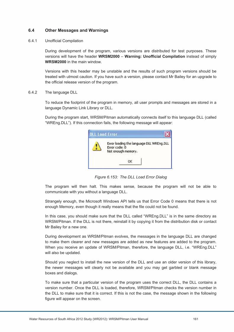
Water Resources of South Africa 2012 Study (WR2012): WRSM/Pitman User Manual 161
6.4 Other Messages and Warnings
6.4.1 Unofficial Compilation
During development of the program, various versions are distributed for test purposes. These versions will have the header WRSM2000 – Warning: Unofficial Compilation instead of simply WRSM2000 in the main window.
Versions with this header may be unstable and the results of such program versions should be treated with utmost caution. If you have such a version, please contact Mr Bailey for an upgrade to the official release version of the program.
6.4.2 The language DLL
To reduce the footprint of the program in memory, all user prompts and messages are stored in a language Dynamic Link Library or DLL.
During the program start, WRSM/Pitman automatically connects itself to this language DLL (called “WREng.DLL”). If this connection fails, the following message will appear:
.
Figure 6.153: The DLL Load Error Dialog
The program will then halt. This makes sense, because the program will not be able to communicate with you without a language DLL.
Strangely enough, the Microsoft Windows API tells us that Error Code 0 means that there is not enough Memory, even though it really means that the file could not be found.
In this case, you should make sure that the DLL called “WREng.DLL” is in the same directory as WRSM/Pitman. If the DLL is not there, reinstall it by copying it from the distribution disk or contact Mr Bailey for a new one.
During development as WRSM/Pitman evolves, the messages in the language DLL are changed to make them clearer and new messages are added as new features are added to the program. When you receive an update of WRSM/Pitman, therefore, the language DLL, i.e. “WREng.DLL” will also be updated.
Should you neglect to install the new version of the DLL and use an older version of this library, the newer messages will clearly not be available and you may get garbled or blank message boxes and dialogs.
To make sure that a particular version of the program uses the correct DLL, the DLL contains a version number. Once the DLL is loaded, therefore, WRSM/Pitman checks the version number in the DLL to make sure that it is correct. If this is not the case, the message shown in the following figure will appear on the screen.

Water Resources of South Africa 2012 Study (WR2012): WRSM/Pitman User Manual 162
Figure 6.154: The Old-DLL Dialog
The program will run after you press the OK button, but especially the newer features of the program will more than likely show blank spaces or errors in the messages and dialogs.
Again you should make sure that the latest version of “WREng.DLL” is in the same folder as WRSM/Pitman. If the DLL is much older than the “WRSM2000.EXE” file, reinstall it by copying it from the distribution disk or contact Mr Allan Bailey for a new one.
6.5 Knowledge Base Articles
Knowledge Base Article1:
How to get the Naturalised flows from a growing and shrinking SFR Child area.
-------------------------------------------------------------------------------------------------------------------------------
For some, it may be of interest to see how afforestation and/or alien vegetation influence the runoff that is generated by an afforested area in an SFR Child. For this, one might want to generate the naturalised runoff for the SFR so that one can compare the reduced runoff with the naturalised runoff.
It would be wrong to run the Child catchment as a separate catchment and then expect that those runoffs could be compared to the runoffs that would be generated by the Child catchment, especially when the area of afforestation (and/or alien vegetation) grows and shrinks.
When one runs the Child SFR as a separate module, the area of the module is constant at the specified area of the catchment. This means that the flows that are created by this means (and stored in the outflow route) would not correspond to a growing and shrinking SFR area.
When an SFR module is run, only that area that is afforested in a given year will generate runoff for the Child. Therefore, if the afforested area grows and shrinks, the runoff that will be generated by the SFR module will be generated from an area that varies in size during the simulation period. All non-afforested and non-alien vegetated area will automatically be assigned to the Parent catchment.
To generate the naturalised flows for an SFR, insert the year/area pairs to describe the growth of the vegetation in the Afforestation dialog of the Child module and select the 'User Defined' SFR option. Now set the required reduction to 0.00% for both Low Flow and MAR.
The program will generate the naturalised flows for the varying size of the catchment that will be covered by the specified vegetated area, but since the reduction is 0.00, the Naturalised flows will be stored in the outflow route of the Child.
One can then save those Child outflows for later use as basis for comparative statistics and graphs.

Water Resources of South Africa 2012 Study (WR2012): WRSM/Pitman User Manual 163
Knowledge Base Article 2:
Surface/groundwater flows split when using CSIR afforestation and Alien vegetation.
-------------------------------------------------------------------------------------------------------------------------------
When using the CSIR afforestation and/or alien vegetation algorithms in a 'normal' catchment while using the Pitman or the Hughes groundwater models, you will notice that there are only zeros in the files that are created by means of the File | Save | Module time series | Runoff Module | Total Surface Runoff or Groundwater Runoff options.
These files will contain values when the there is no CSIR afforestation or Alien vegetation, and also when the Sami groundwater model is used.
The reason for this behaviour is as follows. When either of the CSIR afforestation or alien vegetation routines are used, WRSM/Pitman will first simulate outflows for the catchment in the usual manner, but, as a final step, reduce the final outflows of the catchment according to the relevant CSIR algorithm.
The result is that the split between the surface runoff component and the groundwater runoff component are no longer valid – adding the two flows will no longer produce the total runoff for the catchment. To prevent you from erroneously using these component flows in other programs, such as WQT or WQS which rely on the split between the surface flows and groundwater flows, these files will only contain zero flows. Theoretically, outflows as a result of paved areas are not affected and are therefore reported.
The Sami model is not affected by this, because the Sami model uses the final outflows of a catchment together with the storages as the starting points with which it redistributes flows between surface and groundwater. Since the CSIR reduction is done before the Sami groundwater model runs, the Sami model will produce a split between surface and groundwater outflows. Whether this will produce acceptable results is however a matter of opinion, since the storages that would be used as input would pertain to the situation where afforestation or alien vegetation plays no role.
Should you require a split between surface and groundwater flows for a catchment that has afforestation and you wish to use the CSIR algorithm, we therefore recommend a Parent/Child SFR configuration.
Knowledge Base Article 3:
Surface flow depths for WQS Model (Special version of the WQT Model with code for dealing with mines)
-------------------------------------------------------------------------------------------------------------------------------
It is highly likely that the user will find significant differences between the surface flows depths that are calculated by WQS and by WRSM/Pitman.
As a starting point, WQS uses the outflows of the catchment. Two types of outflow are used in the model: the outflow as a result of the pervious area of the catchment and the outflows that result from the urban area in the catchment.
In this case, the outflows from the urban areas are of no further importance.
Water Resources of South Africa 2012 Study (WR2012): WRSM/Pitman User Manual 164
In WQS, the pervious area outflows are split into groundwater outflows and surface flows by means of hydrograph dissociation. For this, the Mining model of WQS uses a uses 12 monthly defined Minimum base year groundwater flows (SWGMB) to determine the minimum groundwater flow depth for the catchment. If the groundwater flow is greater than the minimum groundwater flow then a lag is calculated for the groundwater by means of a user defined antecedent runoff decay factor (SWRDF). This lagged flow is then released again as an incremental flow, which is governed by a user defined proportion of antecedent flows factor (SWPAF).
WRSM/Pitman uses the simulated surface flows generated in a catchment, discounted by the flows that are generated by any paved area in the catchment.
Clearly the two methods are different. The surface flows that are determined by WRSM/Pitman depend on a good 'fit' between observed and simulated results and the values determined by WQS would depend largely on the values of the parameters that the user supplied.
If differences between the outflows from the mining module are found between WQS and WRSM/Pitman, you should first check the 'fit' of the observed and simulated catchment outflows, and ensure that the two models use the same flows.
In WQS the flows that were dissociated may have been the observed flows. WRSM/Pitman, on the other hand, will always use the simulated outflows.
The flows that are simulated by WRSM/Pitman may deviate from the observed flows depending on the 'goodness of fit' of the calibration. Even though, statistically, the two flows may be virtually identical, there will be localised deviations. Clearly if the observed and simulated flows are not identical, the surface flows that are generated can never be identical.
Knowledge Base Article 4:
Caveats when generating flows for WQT and WQS
-------------------------------------------------------------------------------------------------------------------------------
1. Users of WQS and WQT should use the Runoff module time series 'Total surface outflow' combined with 'Groundwater outflow' for the catchment runoff and 'Paved outflow' for the paved area outflows.
The use of the time series 'Net catchment runoff' should be avoided in this case because this time series contains the flows that are attributed to the catchment discounted by any CSIR afforestation, Alien vegetation and/or Riparian vegetation. This time series would be the same as the total outflow of the catchment through all of the outflow routes, but it would not take any inflows from upstream catchments (as is possible when using the Hughes groundwater model) into account.
2. In WRSM/Pitman, the operations to determine surface and groundwater runoff depths are done before any final stage Riparian vegetation (or CSIR afforestation or Alien vegetation) is deducted from the final outflows of the catchment.
It is acceptable to run a mining module that lies within a 'normal' catchment that has Riparian vegetation or CSIR afforestation or alien vegetation in WRSM/Pitman because the surface runoff and groundwater runoff depths are determined correctly for pervious areas.
However: Should a user enter the outflows from a catchment with Riparian vegetation into WQS, both the pervious area runoff depths and surface runoff depths would be distorted.

Water Resources of South Africa 2012 Study (WR2012): WRSM/Pitman User Manual 165
This is because WQT and WQS both use hydrograph dissociation to determine the runoff depths. The values within the time series 'Total surface outflow' and 'Groundwater outflow' are therefore set to zero (see KB article J2) to stop the user from executing this operation.
3. Although the CSIR afforestation, alien vegetation and Riparian vegetation models only reduce the final outflows of the catchment in 'normal' (i.e. not Parent/Child) catchments, this is not the case in the Van der Zel afforestation routine. The Van der Zel afforestation model reduces the outflows 'at source' which means that the 'Total surface outflows' and 'Groundwater outflow' time series are already discounted by the afforestation. The Van der Zel model should therefore be avoided where the aim is to generate flows for WQT or WQS.
4. In a network that uses the Parent/Child configuration for Stream Flow Reductions, WQT (and WQS) irrigation blocks and mining modules can only lie within a Parent catchment. Because a Parent/Child configuration also reduces outflows 'at source' in the Child catchments, this would falsify the pervious area runoff results. In any event: it is highly unlikely that an irrigation or mining area would lie in the middle of a forest!
Knowledge Base Article 5:
Getting the program to calculate APan factors for the Sami Model.
-------------------------------------------------------------------------------------------------------------------------------
In the Runoff Module, only the Sami Groundwater Model uses APan factors. These Apan factors are derived from the A-pan/S-pan relationship in WR90 Appendix 3 and the standard S-pan factors used in the Climate screen for the Runoff module.
C APAN = Monthly A-pan evaps C FA = Monthly A-pan factors for catchment evap. C DO M = 1 , 12 C where M is month (Oct is 1) IF( (M.EQ.1) .OR. ( M.GE.10 ) ) THEN C For July, August, September and October FA(M) = 0.8 * ( 0.8793 * APAN(M) – 16.2354 ) / APAN(M) ELSE C For all other months FA(M) = ( 0.8793 * APAN(M) – 16.2354 ) / APAN(M) ENDIF END DO
The rules that are followed by WRSM/Pitman are as follows:
a) If there are no Apan factors in the Apan factors input field of the Climate dialog (i.e. all are 0.00) when the Sami model is selected, the program calculates the relevant Apan factors.
b) If the user changes the SPan values, the Apan values and factors are recalculated.
c) If the SPan values are not changed but the APan factors are changed in the Climate dialog, the user-defined factors are used.
If you ever corrupt the APan factors and have forgotten what they should be, you can get the program to calculate them for you again by one of two methods:

Water Resources of South Africa 2012 Study (WR2012): WRSM/Pitman User Manual 166
(a) Change one of the SPan evaporation values to (for example) 3 and press Apply. Then change the value of 3 back to the original value again and press Apply again. I chose 3 rather than 0 because an Span value of 0 will cause an error message that says that one of the evaporation values is suspect, but entering a value of 3 will not. If an evaporation value of 0 is entered, the APan factor will be set to 0 as well.
OR
(b) Change all the Apan factors to 0 and press Apply. Then select any Groundwater model other than the Sami model, press Apply, then select the Sami model again and press Apply.
Knowledge Base Article 6:
The differences between Net and Total return flows from WQT and WQT-SAPWAT Irrigation areas.
-------------------------------------------------------------------------------------------------------------------------------
In the WQT, WQT-SAPWAT and WQT Type v4 Irrigation Modules, it is possible to specify either the 'Net' or 'Total' return flow. The return flows that are generated by the use of these options will seem 'vastly different' at first glance, but in fact the overall difference that this option produces in a network will be very small.
With the 'Total' return flow option activated, the return flows may, in some cases, be higher than the abstractions in the abstraction route of the irrigation block. Some may be tempted to interpret this as a 'magical creation' of flows. This is, however, not the case.
The main difference between 'Net' and 'Total' return flow options is that when the 'Total' return flow option is activated, the runoffs that would be generated by the area if this area were not an irrigation area are also added to the outflows. Corresponding to this, the area of the Runoff module in which the irrigation area lies is decreased. Although the return flows from the irrigation block will therefore be higher, the runoff from the runoff module in which the irrigation block lies will be reduced accordingly.
This can be tested by creating a simple network with a Runoff Module (RU1) that drains into a Channel Reach (CR1) that has two outflow routes: a primary outflow route and an abstraction route to an Irrigation block (RR1). The WQT or WQT-SAPWAT Irrigation block RR1 lies within the Runoff module RU1 and has a return flow route that drains into a second Channel Reach, CR2. The outflows from CR1 are also routed to CR2. A Gauging station is placed on the outflow route from CR2.
Notwithstanding the discourse above:
At the Gauging station of the outflow route to CR2, small differences in flow may be detected whether the 'Net' or 'Total' return flow option is chosen in the Irrigation block RR1.
In a run-of-river irrigation scheme such as the one described above, the differences in flows that do occur are the result of routing.
A 'Net' irrigation block does not reduce the area of the catchment in which it lies. Therefore, especially during low flows, more flow would enter CR1 from the Runoff Module, from where the Irrigation Block RR1 could abstract it. A comparison of the flows in the abstraction route would bear this out: when an irrigation block is a 'Net' return flow block it will abstract slightly more water

Water Resources of South Africa 2012 Study (WR2012): WRSM/Pitman User Manual 167
than a 'Total' return flow irrigation block. It is important to note that this higher abstraction occurs at times when the supply is failing.
Because of the slightly higher abstraction, the crops in a 'Net' irrigation block can use slightly more water, hence one would expect that the return flows would be slightly less – when corrected for the pervious runoff component that is added to a 'Total' outflow return flow, of course.
This is borne out by a comparison of the outflows that are simulated at the Gauging station at the outflow of Channel Reach CR2 (which collects the outflows from Channel Reach 1 and the Return Flows from RR1). During periods of low flow, the flows produced downstream of a 'Total' return flow irrigation block are slightly higher than those produced by a 'Net' return flow irrigation block. A 'Net' return flow irrigation block is therefore slightly 'thirstier' than a 'Total' return flow irrigation block.
It should be borne in mind, though, that this effect only becomes apparent when the supply to the irrigation scheme is failing, which, in itself is a highly undesirable state of affairs.

Water Resources of South Africa 2012 Study (WR2012): WRSM/Pitman User Manual 168
7 DOs and DON'Ts
7.1 DO:
Solve runoff modules before their outflows are required.
Solve irrigation blocks before their supply modules.
Be careful when specifying that a module should not be solved – the program will not be able to solve any of the downstream modules, since the flows in the outflow routes will not have been determined.
Start with a small network and build it up slowly once the simple network works.
Think in terms of objects when designing your network – for example: the flows in an abstraction route from a reservoir should be seen as part of a reservoir, not as part of some downstream module. Although it is not "wrong" to use reverse logic (except in the case of compensation releases from reservoirs – see below) you can easily become confused by it.
7.2 DON'T:
Connect an irrigation block directly to a Runoff model. This will give an answer, but it will be wrong because all outflows from the Runoff model will be forced through the Irrigation block. Rather connect the irrigation block to a channel reach module into which a Runoff model drains. In that way the irrigation block can abstract what it needs (or can).
Define the flows in the PRINCIPAL outflow route of a channel reach. Although this is possible, it should be avoided. If more water is available than is catered for in the primary outflow route, the channel reach will 'lose' the water, and if less water is available, an error message is generated and water will be 'created' to match the defined flow. Clearly neither is correct. Rather use two routes, define one, and let the model take care of the other.
Define flows unless you absolutely have to. Rather allow the model to do the calculations for you.
Use a combined spillage / compensation flows route from a reservoir if you are interested in the figures for 'actual draft' in the reservoir plots. If these routes are combined, the spillages will be added to the compensation releases already in the route, which will then be used to determine the total actual draft. This is clearly not correct. Although it is possible to combine them, rather use separate routes for spillages and compensation releases. The program will ignore the flows in a dedicated spillage route when actual drafts are calculated, but cannot ignore it if spillages are combined with defined compensation outflows.
Use WRSM/Pitman to calculate design floods for weirs bridges and other structures. WRSM/Pitman is a monthly model, and it therefore reports MONTHLY flows AVERAGED for a particular month. It is therefore theoretically possible (though unlikely) that the total monthly flow could have passed through a route all in one minute, one hour, one day, one week or any time span that you may wish to think of that is less than or equal to one month. Use a different model to determine design floods.

Water Resources of South Africa 2012 Study (WR2012): WRSM/Pitman User Manual 169
8 DEFICIT HANDLING
Deficits due to excessive abstractions.
From time to time, it may happen that a module cannot supply the water that is demanded from it. This can occur where an irrigation module draws water from either a reservoir or a channel reach module. Another possible cause is where there is a defined demand on either a reservoir or a channel reach. In the event that too little water is available, the following distribution of available water is affected:
• defined routes are satisfied, if at all possible;
• water is sent to non-defined (i.e. calculated) irrigation abstraction routes and monthly defined abstraction routes, in amounts proportional to the demand. Irrigation blocks have preference over outflow and spillage routes, unless these are defined flow routes and
• the return flows from irrigation blocks are adjusted to correspond with the new (reduced) inflow.
Note that if step 1 uses all the resources, the redistribution of demands for step 2 will not be attempted, and flows in affected calculated routes will be set to 0. Return flows for step 3 will then also be set to zero.
The flows in DEFINED routes are NEVER adjusted downwards, and the flows in only one type of defined route will be adjusted upwards. Even if a reservoir or channel reach is bone dry, but a defined flow is given for an outflow route, that route will carry the full defined flow. The ONLY defined route in which flows will be adjusted upwards is the case where a defined releases route doubles as a spillage route in a reservoir module. In this case, spillages are ADDED to the defined releases. If there is a deficit, the spillages (if any) are adjusted downwards, but the DEFINED portion of the flow remains inviolate. This was done because the defined route flows are assumed to be historical data. If your network cannot cope with historical data, the network should be adjusted, and not the historical data. If spillages are added to a defined reservoir release, the upwardly adjusted flows will be valid only for the duration of the run in question. Once the network is run again, (e.g. with changed runoff parameters) the original defined releases are used.
At the end of the simulation, messages will appear on the screen if demands could not be met, telling the user to check his error file. In this file the number and name of the module (Reservoir or Channel Reach) in which the deficit occurred is reported, e.g.
Channel Reach (reach number) (reach name)
At least one xxxxx failure to supply defined demands
At least one xxxxx failure to supply calculated demands.
Reservoir (reservoir number) (reservoir name)
At least one xxxxx failure to supply defined demands.
At least one xxxxx failure to supply calculated demands
where xxxxx can be either "minor" or "major".
If the program reports only:

Water Resources of South Africa 2012 Study (WR2012): WRSM/Pitman User Manual 170
At least one xxxxx failure to supply calculated demands
for a module that has both defined and non-defined routes, it means that the defined routes were satisfied, but not the non-defined (or calculated) routes. If a module has both defined and non-defined routes, the amount of water available for redistribution to non-defined routes is first calculated by subtracting the flows to the defined routes from the total amount available.
The outflow to non-defined routes is set to the proportion of the demand that is available. For example: if route 1 demands 2.5 million m³ and route 2 demands 3 million m³ (total demand 5.5 million m³) but only 3.5 million m³ is available, route 1 will receive ( 2.5 * 3.5 / 5.5 = ) 1.59 million m³ (rounded to 2 significant digits) and route 2 will receive ( 3.0 * 3.5 / 5.5 = ) 1.91 million m³ (also rounded to 2 significant digits.)
If there is a message that states that for a specific Reservoir or Channel Reach:
At least one xxxxx failure to supply defined demands
This means that the defined outflows were larger than what the module (Channel Reach or Reservoir) could deliver. If the module has both defined and non-defined routes, a message will also appear that the calculated demands could not be met – since if defined routes with the higher priority cannot be met, the calculated route flows will also not be met. In this case the calculated route flows will be set to 0.
In the event that defined routes cannot be satisfied, the maximum possible flow that could be supplied to these defined routes is calculated. Once again, if there are two or more defined routes that vie for an insufficient amount of water, the amount that could be supplied to the routes is shared out proportional to the demand that was originally specified.
This maximum supply (and the demand and the shortages) can be inspected by creating output files by means of the File | Save | Route Flows menu point.
During execution, the message:
Redistribution failed. Redistributed flow: ____ Available ___
This is a last-ditch error message, and (with luck) we will probably never see it. It means that the redistribution algorithm has broken down. After redistributing the flows, a check is made to see whether water was either created or destroyed in the redistribution process. If water was created or destroyed, this is the error message that will be seen.
When a deficit is found for a defined route, the flows in the route are NOT adjusted, because defined route flows are inviolate. Only abstractions to non-defined routes are adjusted.
If you get many of these error messages, there is something seriously wrong with your network.
Hint: An alternative way to observe the difference between supply and demand is to run the model with an abundant supply of water and store the affected routes in “.ANS” files. Then adjust the model by adding a Gauging Station on the Irrigation abstraction route and using the files created above as the Gauging Station time series. The monthly hydrograph can then be used to show the differences graphically.
Special case: Monthly defined abstractions from reservoirs.
If a reservoir has not yet been built, it has a storage volume of 0. If a simulation runs from 1920 until 1987, and the reservoir is only commissioned in 1948, there will be a storage of 0 from 1920

Water Resources of South Africa 2012 Study (WR2012): WRSM/Pitman User Manual 171
until the dam is built in 1948. The result is that monthly defined abstractions (if specified) will be reduced by the restriction factor until the water in the reservoir has accumulated to more than the defined minimum storage level.

Water Resources of South Africa 2012 Study (WR2012): WRSM/Pitman User Manual 172
9 DEFAULT PARAMETERS
WRSM/Pitman has evolved into a complex model requiring a large number of input variables or parameters. The effort involved in the determination of these input variables for even a simple network is considerable. Accordingly, default values for many of the variables have been established, in order to make it easier for the user to begin running the model. Naturally it has not been feasible to provide defaults for every single input variable. For example, all areas required by the model are left equal to zero. This makes sense when the areas refer to areas affected by a particular land use, thus defaulting to the zero land use or virgin catchment situation.
It should be possible to run the model with all defaults (apart from areas) in place but many of the parameters will obviously have to be changed to obtain a reasonable simulation of one’s particular network. Some of the defaults would not normally need to be changed, whereas some defaults are merely reasonable values that would not cause the program to give error messages. In the light of the foregoing, three categories of default are recognized, as described below.
9.1 Categories of default input variables/parameters
The enhanced WRSM/Pitman model has three colours in the data requirements for calibration, Sami and Hughes parameters as follows:
• category 1 parameters that should normally never be changed (red in WRSM/Pitman model);
• category 2 parameters that can be changed but the defaults given are probably the best estimates (blue in WRSM/Pitman model) and
• category 3 parameters where only a realistic value is given for the default. One would normally change most of these values once the program is running (white in WRSM/Pitman model).
The tables on the following pages list all defaults by module type and input screen. In addition to the default category, notes are given as a further aid to the user when altering (or leaving unchanged) the parameters in question. Where defaults are zero (mainly for areas but also for other variables where appropriate) they have not been included, unless they are parameters of the runoff model.

Wat
er R
esou
rces
of S
outh
Afri
ca 2
012
Stu
dy (W
R20
12):
WR
SM
/Pitm
an U
ser M
anua
l 17
3
Tabl
e 9.
1:
Def
ault
Info
rmat
ion
for D
ata
and
Sam
i and
Hug
hes
Par
amet
ers
Mod
ule
Scr
een
Var
iabl
e D
efau
lt C
ateg
ory
Not
es
Run
off
Clim
ate
MA
P
700
3 R
easo
nabl
e av
erag
e fo
r SA
Eva
pora
tion
100
(x12
) 3
Zero
def
aults
wou
ld b
e un
real
istic
Cal
ibra
tion
S p
an fa
ctor
s 0.
8, 1
.0 (x
8), 0
.8 (x
3)
3 D
on’t
chan
ge, u
nles
s yo
u w
ant t
o us
e an
othe
r typ
e of
pan
PO
W*
3 3
Usu
ally
1 (r
arel
y), 2
(som
etim
es) o
r 3 (o
ften)
GPO
W
3 2
Rec
omm
ende
d by
Hug
hes
& S
ami
SL*
0
1 N
ot re
com
men
ded
to c
hang
e
HG
SL
0 3
Rec
omm
ende
d by
Hug
hes
& S
ami
ST*
15
0 3
Rea
sona
ble
first
est
imat
e
FT*
20
2 R
easo
nabl
e fir
st e
stim
ate
GW
* 0
3 U
sed
only
whe
re b
asef
low
is s
trong
HG
GW
2
3 R
easo
nabl
e fir
st e
stim
ate
ZMIN
* 99
9 3
Nor
mal
ly in
eas
tern
SA
whe
re S
T <
300
ZMA
X*
999
3 N
orm
ally
in e
aste
rn S
A w
here
ST
< 30
0
PI*
1.
5 3
Don
’t ch
ange
unl
ess
high
% n
atur
al fo
rest
TL*
0.25
3
Goo
d av
erag
e
GL*
2.
5 2
Use
d on
ly if
GW
> 0
R*
0.5
2 W
orks
bes
t for
all
area
s ex
cept
win
ter r
ainf
all
TLG
Max
2
2 R
ecom
men
ded
by H
ughe
s
Reg
iona
l GW
gra
dien
t 0.
01
2 R
ecom
men
ded
by H
ughe
s
* P
itman
par
amet
ers
- -
Ref
er to
WR
90 fo
r bes
t ini
tial e
stim
ates
H
ughe
s G
W
Dra
inag
e de
nsity
0.
4 2
Rec
omm
ende
d by
Hug
hes
Rip
aria
n zo
ne (R
Z)
40%
2
Rec
omm
ende
d by
Hug
hes
Upp
er z
one
60%
2
Rec
omm
ende
d by
Hug
hes
Rip
aria
n st
rip (%
RZ)
0.
2%
3 R
ecom
men
ded
by H
ughe
s
Sto
rativ
ity
0.00
1 3
Rea
sona
ble
aver
age
Tran
smis
sivi
ty
10
3 R
easo
nabl
e av
erag
e
Res
t wat
er le
vel
20
3 R
easo
nabl
e av
erag
e
Sam
i GW
A
quife
r thi
ckne
ss
20
3 R
easo
nabl
e av
erag
e

Wat
er R
esou
rces
of S
outh
Afri
ca 2
012
Stu
dy (W
R20
12):
WR
SM
/Pitm
an U
ser M
anua
l 17
4
Mod
ule
Scr
een
Var
iabl
e D
efau
lt C
ateg
ory
Not
es
Sto
rativ
ity
0.00
5 3
Rea
sona
ble
aver
age
Initi
al a
quife
r sto
rage
0.
9 *
aqui
fer
capa
city
(st
orat
ivity
* a
quife
r th
ickn
ess
* 10
00).
45 if
no
info
3
Rea
sona
ble
aver
age
Sta
tic w
ater
leve
l 60
3
Rea
sona
ble
aver
age
Max
. dis
char
ge ra
te
2 2
Rea
sona
ble
aver
age
Pow
er
-0.0
5 1
Usu
ally
not
cha
nged
Max
. hyd
raul
ic g
rad.
0.
001
2 R
easo
nabl
e av
erag
e
GW
eva
pora
tion
area
(1
% a
rea)
2
Rea
sona
ble
aver
age
– ca
n be
up
to 5
%
Mon
ths
ave.
rech
arge
2
2 R
easo
nabl
e av
erag
e –
muc
h gr
eate
r for
dol
omite
s
Uns
at. S
tora
ge c
ap.
20
3 R
easo
nabl
e av
erag
e
Initi
al u
nsat
. Sto
rage
10
3
Usu
ally
set
to h
alf c
apac
ity
Per
cola
tion
pow
er
0.2
1 U
sual
ly n
ot c
hang
ed
Tran
smis
sivi
ty
10
3 R
easo
nabl
e av
erag
e
Bor
ehol
e di
st. T
o riv
. 10
00
3 R
easo
nabl
e av
erag
e
Par
amet
er K
2 0.
1 2
Onl
y im
porta
nt w
here
abs
tract
ions
take
pla
ce
Par
amet
er K
3 -3
2
Onl
y im
porta
nt w
here
abs
tract
ions
take
pla
ce
Inte
rflow
lag
0 2
Usu
ally
not
cha
nged
Affo
rest
atio
n
Rot
atio
n le
ngth
15
2
Nee
ded
only
for C
SIR
% o
ptim
um g
row
th
50
2 N
eede
d on
ly fo
r CS
IR
Age
(all
type
s)
20
2 R
easo
nabl
e es
timat
e if
no d
ata
avai
labl
e
Alie
n ve
g.
% o
ptim
um g
row
th
50
2 A
s fo
r affo
rest
atio
n
Rip
aria
n %
0
3 A
ssum
e al
l upl
and
initi
ally
Res
ervo
ir C
limat
e
MA
P
700
3 R
easo
nabl
e av
erag
e fo
r SA
Eva
pora
tion
100
(x12
) 3
Zero
def
aults
wou
ld b
e un
real
istic
Pan
fact
or
0.81
,0.8
2,0.
83,
1 D
on’t
chan
ge, u
nles
s yo
u w
ant t
o us
e an
othe
r typ
e of
pan
Sto
rage
P
ower
vol
./are
a cu
rve
0.84
,0.8
8…et
c.0.
60
2 C
hang
e if
area
/vol
ume
data
ava
ilabl
e
Irrig
atio
n C
limat
e
MA
P
700
3 R
easo
nabl
e av
erag
e fo
r SA
Eva
pora
tion
100
(x12
) 3
Zero
def
aults
wou
ld b
e un
real
istic
Pan
fact
or
0.6,
0.8.
.etc
. 2
Con
verte
d fro
m S
-pan
to A
-pan
(see
runo
ff)
Rai
nfal
l fac
tors
0.
75 (x
12)
2 G
ener
ally
acc
epte
d as
bei
ng re
alis
tic

Wat
er R
esou
rces
of S
outh
Afri
ca 2
012
Stu
dy (W
R20
12):
WR
SM
/Pitm
an U
ser M
anua
l 17
5
Mod
ule
Scr
een
Var
iabl
e D
efau
lt C
ateg
ory
Not
es
Max
imum
rain
fall
fact
ors
0 (x
12)
2 W
QT
Type
4
Cro
ps(o
ld m
odel
) P
inde
x (x
12)
2 Fo
r cas
e w
here
full
area
irrig
ated
yea
r-ro
und
Effe
ctiv
e ra
in fa
ctor
s 0.
75 (x
12)
2 G
ener
ally
acc
epte
d as
bei
ng re
alis
tic
Allo
catio
n
Net
allo
catio
n (m
m)
9999
2
Arb
itrar
ily la
rge
valu
e fo
r no
allo
catio
n lim
it
Net
allo
c. (M
CM
) 99
99
2 A
rbitr
arily
larg
e va
lue
for n
o al
loca
tion
limit
Allo
catio
n gr
owth
(a
ll ye
ars)
2
No
chan
ge in
allo
catio
n ov
er ti
me
Cro
ps2(
WQ
T,
WQ
T-S
AP
WA
T an
d W
QT
Type
4
mod
els)
Cro
p de
man
d fa
ctor
s 0.
74,…
.etc
. 3
Def
aults
are
for s
ugar
can
e
Eff.
Rai
nfal
l lim
it 1
100
2 R
ecom
men
ded
by H
erol
d
Eff.
rain
fall
limit
2 0
2 R
ecom
men
ded
by H
erol
d
Can
al
Pro
p.
lost
to
se
epag
e an
d ev
apor
atio
n 0
2 D
efau
lt is
no
cana
l
Pro
p.
Tran
smis
sion
lo
st
to
evap
orat
ion
0 2
WQ
T Ty
pe 4
. Def
ault
is n
o ca
nal
Pro
p. s
eep.
Ret
urne
d to
rive
r 0
2 D
efau
lt is
no
cana
l
Pro
p. I
rrig
atio
n su
pply
spi
lled
from
ca
nal e
nds
0
WQ
T Ty
pe 4
. Def
ault
is n
o ca
nal
Gro
undw
ater
Upp
er z
one
stor
age
400
2 R
ecom
men
ded
by H
erol
d
Low
er z
one
stor
age
1000
2
Rec
omm
ende
d by
Her
old
Initi
al S
M s
tora
ge
250
2 R
ecom
men
ded
by H
erol
d
Targ
et S
M s
tora
ge
250
2 R
ecom
men
ded
by H
erol
d
Pro
p. re
turn
flow
:Upp
er z
one
0.75
2
Rec
omm
ende
d by
Her
old
Low
er z
one
0.25
2
Rec
omm
ende
d by
Her
old
Upp
er s
oil z
one
max
imum
sto
rage
70
0 2
Rec
omm
ende
d by
Her
old
Upp
er s
oil z
one
min
imum
sto
rage
0
2 R
ecom
men
ded
by H
erol
d
Loss
to d
eep
seat
ed g
roun
dwat
er
0 2
Rec
omm
ende
d by
Her
old
Effi
cien
cy
Effi
cien
cy fa
ctor
0.
85
2 E
ffici
ency
for c
entre
piv
ot
Effi
cien
cy g
row
th
(all
year
s)
2 N
o ch
ange
in e
ffici
ency
ove
r tim
e
Ret
urn
flow
s
% a
bstra
ctio
n (o
ld)
10
2 Ty
pica
l est
imat
e
Fact
or (
WQ
T, W
QT-
SA
PW
AT
and
WQ
T Ty
pe 4
) 0.
02
2 Yi
elds
abo
ut 1
0% a
bstra
ctio
n on
ave
rage
Gro
wth
in re
t. Fl
ow
1.0
(all
year
s 2
No
chan
ge in
fact
or (o
r per
cent
age)
ove
r tim
e
Irrig
atio
n C
apac
ity
Cap
acity
of w
ater
infra
stru
ctur
e 0
(all
year
s)
2 W
QT
Type
4

Wat
er R
esou
rces
of S
outh
Afri
ca 2
012
Stu
dy (W
R20
12):
WR
SM
/Pitm
an U
ser M
anua
l 17
6
Mod
ule
Scr
een
Var
iabl
e D
efau
lt C
ateg
ory
Not
es
Cha
nnel
Clim
ate
MA
P
700
3 R
easo
nabl
e av
erag
e fo
r SA
Eva
pora
tion
100
(x12
) 3
Zero
def
aults
wou
ld b
e un
real
istic
Pan
fact
or
0.81
,0.8
2,0.
83,0
.84,
0.88
…et
c.
1 D
on’t
chan
ge, u
nles
s yo
u w
ant t
o us
e an
othe
r typ
e of
pan
Wet
land
s (B
) R
echa
rge
coef
ficie
nt
1.0
2 U
se fo
r wet
land
(low
er c
oeff.
for a
quife
r)
Wet
land
s (C
) P
ower
are
a/vo
l. E
qn.
0.6
2 U
nlik
ely
to h
ave
area
/vol
ume
data

Water Resources of South Africa 2012 Study (WR2012): WRSM/Pitman User Manual 177
10 CALIBRATION
Once all the data has been entered into the various modules and routes, the graphs and statistics are used to check on the calibration between simulated and observed (known) streamflow and storage. Streamflow can be checked at any route where there are observed streamflows (denoted by Obs **** and the gauge description). The simulated storage in reservoirs can also be checked against observed storage. If the WR2012 network systems are downloaded from the website, the calibrations have already been carried out.
10.1 Surface water component calibration
Step 1:Statistics
For the surface water component calibration, it is advisable to firstly set the mode to Pitman in the runoff modules as there are tips given in the Statistics screen on how to improve on the calibration. Figure 10.1 shows a statistics screen for a route that contains an observed streamflow record. For each statistical parameter, there is a tip on how it can be improved on the right-hand side. For “seasonal index” there are two rows of tips, some for increasing a parameter and the other for decreasing. Finally there is a block at the bottom that suggests parameter changes that should improve all the statistical parameters. Note that there could be a conflict in that one statistical parameter may have a tip to increase a parameter while another may be to decrease the same parameter. In Figure 10.1 there is a tip on MAR to increase Zmin while for the “log std deviation” the tip is to decrease Zmin. In such a conflict, one has to look first at MAR, then standard deviation and lastly seasonal index as the degree of importance.
Try to obtain a good fit on observed statistics. There are no firm criteria as to what constitutes a "good fit” but one can use the following guidelines:
• Error in MAR and mean (log): < 4% • Error in std. dev (natural & log): < 6% • Error in seasonal index: < 8%
It is recommended that the user change only one parameter at a time.
After a number of runs you will either get the message "SORRY, NO FURTHER SUGGESTIONS ….." at the bottom of the screen or you may feel that any further adjustments to parameters will not improve the statistics to any significant degree. This is a good time to have a look at the plots on the screen and do some fine tuning.
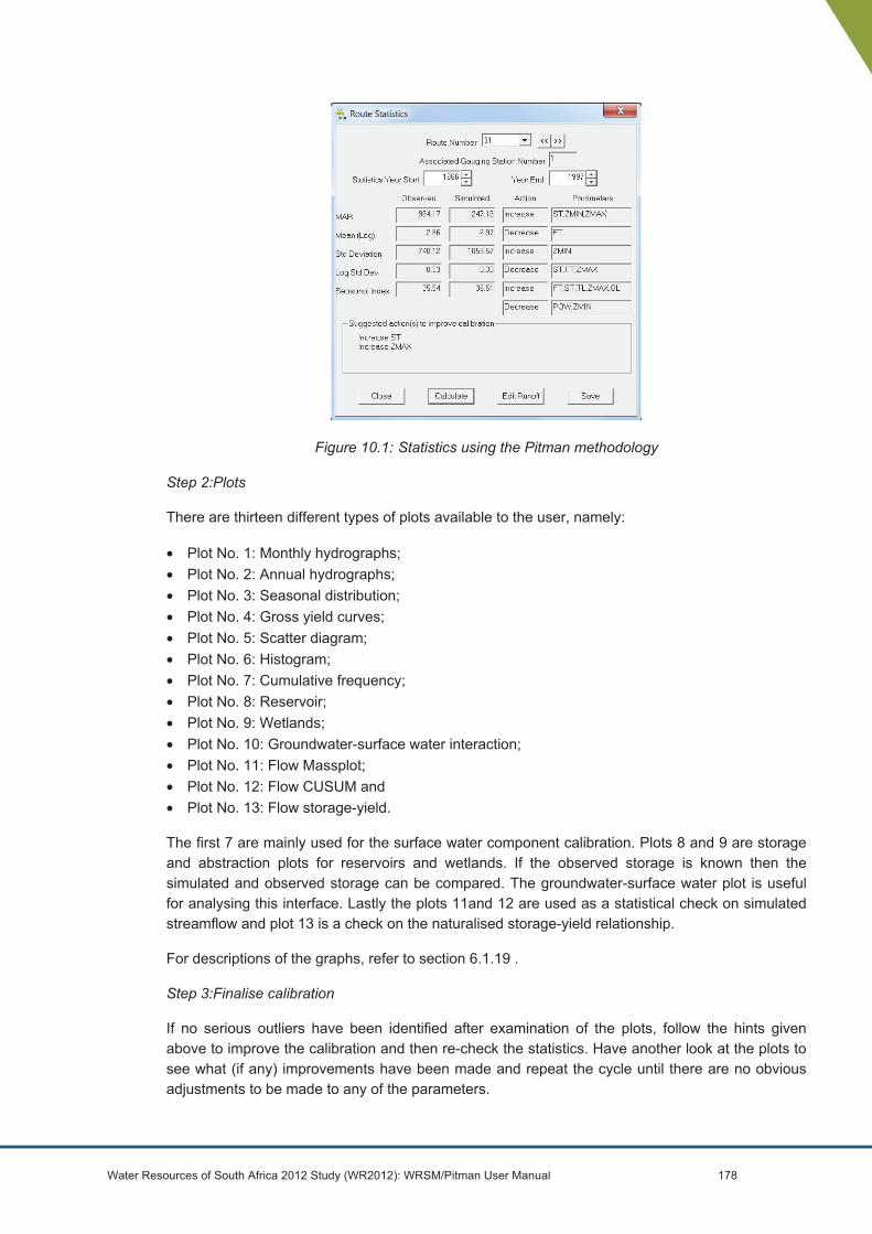
Water Resources of South Africa 2012 Study (WR2012): WRSM/Pitman User Manual 178
Figure 10.1: Statistics using the Pitman methodology
Step 2:Plots
There are thirteen different types of plots available to the user, namely:
• Plot No. 1: Monthly hydrographs; • Plot No. 2: Annual hydrographs; • Plot No. 3: Seasonal distribution; • Plot No. 4: Gross yield curves; • Plot No. 5: Scatter diagram; • Plot No. 6: Histogram; • Plot No. 7: Cumulative frequency; • Plot No. 8: Reservoir; • Plot No. 9: Wetlands; • Plot No. 10: Groundwater-surface water interaction; • Plot No. 11: Flow Massplot; • Plot No. 12: Flow CUSUM and • Plot No. 13: Flow storage-yield.
The first 7 are mainly used for the surface water component calibration. Plots 8 and 9 are storage and abstraction plots for reservoirs and wetlands. If the observed storage is known then the simulated and observed storage can be compared. The groundwater-surface water plot is useful for analysing this interface. Lastly the plots 11and 12 are used as a statistical check on simulated streamflow and plot 13 is a check on the naturalised storage-yield relationship.
For descriptions of the graphs, refer to section 6.1.19 .
Step 3:Finalise calibration
If no serious outliers have been identified after examination of the plots, follow the hints given above to improve the calibration and then re-check the statistics. Have another look at the plots to see what (if any) improvements have been made and repeat the cycle until there are no obvious adjustments to be made to any of the parameters.

Water Resources of South Africa 2012 Study (WR2012): WRSM/Pitman User Manual 179
If any outliers have been identified in step 2 (especially via plot nos. 1, 2 and 5) then edit your file of observed flows and extract the largest portion of record that does not contain any outliers and calibrate on this period. Note that it is possible to check the statistics on any portion of the observed record. You can, therefore, check the statistics on part of the record before editing the file of observed flows.
Table 10.1 gives some useful information and advice on calibration using the Pitman method.
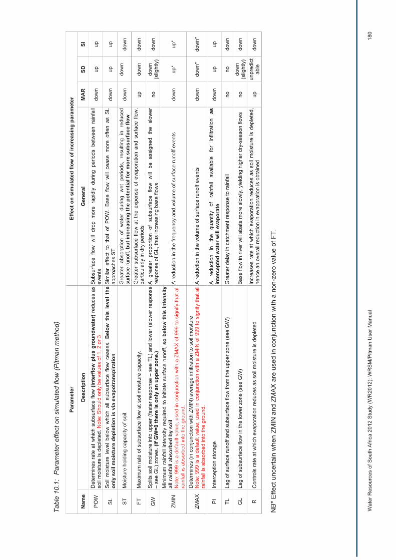
Wat
er R
esou
rces
of S
outh
Afri
ca 2
012
Stu
dy (W
R20
12):
WR
SM
/Pitm
an U
ser M
anua
l 18
0
Tabl
e 10
.1:
Par
amet
er e
ffect
on
sim
ulat
ed fl
ow (P
itman
met
hod)
Para
met
er
Effe
ct o
n si
mul
ated
flow
of i
ncre
asin
g pa
ram
eter
Nam
e D
escr
iptio
n G
ener
al
MA
R
SD
SI
PO
W
Det
erm
ines
rat
e at
whi
ch s
ubsu
rface
flow
(int
erflo
w p
lus
grou
ndw
ater
) red
uces
as
soil
moi
stur
e is
dep
lete
d. N
ote:
Sho
uld
only
be
valu
es o
f 1, 2
or 3
S
ubsu
rface
flo
w w
ill d
rop
mor
e ra
pidl
y du
ring
perio
ds b
etw
een
rain
fall
even
ts
dow
n up
up
SL
Soi
l m
oist
ure
leve
l be
low
whi
ch a
ll su
bsur
face
flo
w c
ease
s. B
elow
thi
s le
vel
the
only
soi
l moi
stur
e de
plet
ion
is v
ia e
vapo
tran
spira
tion
Sim
ilar
effe
ct t
o th
at o
f P
OW
. B
ase
flow
will
cea
se m
ore
ofte
n as
SL
appr
oach
es S
T do
wn
up
up
ST
Moi
stur
e ho
ldin
g ca
paci
ty o
f soi
l G
reat
er a
bsor
ptio
n of
wat
er d
urin
g w
et p
erio
ds,
resu
lting
in
redu
ced
surfa
ce ru
noff,
but
incr
easi
ng th
e po
tent
ial f
or m
ore
subs
urfa
ce fl
ow
dow
n do
wn
dow
n
FT
Max
imum
rate
of s
ubsu
rface
flow
at s
oil m
oist
ure
capa
city
. G
reat
er s
ubsu
rface
flo
w a
t th
e ex
pens
e of
eva
pora
tion
and
surfa
ce f
low
, pa
rticu
larly
in d
ry p
erio
ds
up
dow
n do
wn
GW
S
plits
soi
l moi
stur
e in
to u
pper
(fas
ter r
espo
nse
– se
e TL
) and
low
er (s
low
er re
spon
se
– se
e G
L) z
ones
. (If
GW
=0 th
ere
is o
nly
an u
pper
zon
e.)
A g
reat
er p
ropo
rtion
of
subs
urfa
ce f
low
will
be
assi
gned
the
slo
wer
re
spon
se o
f GL,
thus
incr
easi
ng b
ase
flow
s no
do
wn
(slig
htly
) do
wn
ZMIN
Min
imum
rai
nfal
l int
ensi
ty r
equi
red
to in
itiat
e su
rface
run
off,
so b
elow
this
inte
nsity
al
l rai
nfal
l abs
orbe
d by
soi
l N
ote:
999
is a
def
ault
valu
e, u
sed
in c
onju
nctio
n w
ith a
ZM
AX
of 9
99 to
sig
nify
that
all
rain
fall
is a
bsor
bed
into
the
grou
nd.
A re
duct
ion
in th
e fre
quen
cy a
nd v
olum
e of
sur
face
runo
ff ev
ents
do
wn
up*
up*
ZMA
X
Det
erm
ines
(in
conj
unct
ion
with
ZM
IN) a
vera
ge in
filtra
tion
to s
oil m
oist
ure
Not
e: 9
99 is
a d
efau
lt va
lue,
use
d in
con
junc
tion
with
a Z
MIN
of 9
99 to
sig
nify
that
all
rain
fall
is a
bsor
bed
into
the
grou
nd.
A re
duct
ion
in th
e vo
lum
e of
sur
face
runo
ff ev
ents
do
wn
dow
n*
dow
n*
PI
Inte
rcep
tion
stor
age
A
redu
ctio
n in
th
e qu
antit
y of
ra
infa
ll av
aila
ble
for
infil
tratio
n as
in
terc
epte
d w
ater
will
eva
pora
te
dow
n up
up
TL
Lag
of s
urfa
ce ru
noff
and
subs
urfa
ce fl
ow fr
om th
e up
per z
one
(see
GW
) G
reat
er d
elay
in c
atch
men
t res
pons
e to
rain
fall
no
no
dow
n
GL
Lag
of s
ubsu
rface
flow
in th
e lo
wer
zon
e (s
ee G
W)
Bas
e flo
w in
rive
r will
aba
te m
ore
slow
ly, y
ield
ing
high
er d
ry-s
easo
n flo
ws
no
dow
n (s
light
ly)
dow
n
R
Con
trols
rate
at w
hich
eva
pora
tion
redu
ces
as s
oil m
oist
ure
is d
eple
ted
Incr
ease
s ra
te a
t whi
ch e
vapo
ratio
n re
duce
s as
soi
l moi
stur
e is
dep
lete
d,
henc
e an
ove
rall
redu
ctio
n in
eva
pora
tion
is o
btai
ned
up
unpr
edic
tab
le
dow
n
NB
* Effe
ct u
ncer
tain
whe
n ZM
IN a
nd Z
MA
X a
re u
sed
in c
onju
nctio
n w
ith a
non
-zer
o va
lue
of F
T.

Water Resources of South Africa 2012 Study (WR2012): WRSM/Pitman User Manual 181
Order of Importance of parameter adjustments are given in the following two tables
Table 10.2: Perennial rivers (sub-surface flow important)
ST : Most important (affects MAR, SD and SI)
FT :
TL :
GW : Important for hydrograph shape (SI)
GL :
POW : Change if FT, GW, GL do not yield satisfactory hydrograph shape (SI)
ZMIN : Of importance when FT approaches zero and also when
ZMAX : ST is large (say ≥ 200 mm)
SL :
PI : Try to avoid adjusting these
R :
Table 10.3: Intermittent rivers (sub-surface flow insignificant)
ZMIN : Most important (MAR, SD)
ZMAX :
ST : Make large enough such that any further increase has no effect
TL : Important for hydrograph shape (SI)
POW :
FT :
GW : Should all be set to zero
GL :
SL :
PI : Do not adjust
R :

Water Resources of South Africa 2012 Study (WR2012): WRSM/Pitman User Manual 182
10.2 Groundwater component calibration
Table 10.4 gives some useful information and advice on calibration using the Sami method.
Table 10.4: Effects on simulated flows of model parameter adjustments (Sami method)
Decrease MAR SD SI
FT down down up
POW up up down
ZMAX up up up
ST up up up
ZMIN up up up
HGSL up up down
max Q down down up
HGGW down down up
GPOW up up down
SWL up down down
WRSM/Pitman has a number of groundwater variables that are required for the “Sami” screen such as aquifer thickness, storativity, transmissivity, etc. Some of these generally remain the same from catchment to catchment but most of them differ across catchments. Many of these have starting default values provided in (Sami, 2015) Appendix 1. Others are intuitive based on standard hydrogeological conceptualisations of a system and are discussed under groundwater calibration
In the “Calibration” screen there are also parameters that are only required for the Sami groundwater/surface water methodology as follows:
• GPOW; • HGGW and • HGSL.
Other calibration parameters also have an effect on some groundwater parameters.
The user can assess the groundwater issues by examining the groundwater graph (“Plot” screen) as well as printing out time series data for various monthly groundwater parameters (“File” screen). The following time series can be written to datafiles:
• Groundwater outflows (for the Hughes method it is discharge, for Sami it is groundwater baseflow plus interflow);
• Pitman S (mm) for Sami only (Pitman S is the time series of variation in soil moisture from 0 to a value of ST);
• Weighted Pitman S (mm) Sami only; • Aquifer storage (mm) for Sami only; • Aquifer recharge (mm) for Sami only; • Groundwater baseflows (discharge) for Sami only; • Interflows for Sami only and • Total recharge (aquifer recharge plus interflow) (mm) for Sami only.

Water Resources of South Africa 2012 Study (WR2012): WRSM/Pitman User Manual 183
The final variable requires some explanation. If the user is analysing naturalised flows, i.e. the runoff “tickbox” for naturalised flows is checked, then child modules have no effect as afforestation and alien vegetation are ignored. Therefore the “Total recharge” for the parent runoff module is all that needs to be determined for the purposes of calibrating recharge against other recharge data like the GRAII study (DWS study completed in 2005). This “Total recharge” is the aquifer recharge (mm/month) plus the interflow converted to mm/month (by dividing by the parent catchment area and multiplied by 1000 to get mm/month). For the non-naturalised situation where data on recharge reduction is required, like to determine the impacts of afforestation, alien vegetation or sugar cane on recharge, it is more involved. WRSM/Pitman in this case calculates groundwater parameters for both the parent and child modules. So the “Total Recharge” time series for both the parent and child modules must be determined. The same applies to “Aquifer recharge”. The “Total recharge” for the catchment must then be determined by area weighting the parent and child values (as they are in mm). For the “Interflows”, the parent and child should be added (as they are in million m3/month).
The following serves as an example where of a catchment area of 58 km2, 50 km2 is afforestation (constant from 1920 to 2009).
Table 10.5: Groundwater variable analysis for “total recharge”
Analysis Catchment
area (km2)
Interflow(million
m3/a)
Surface runoff
(million m3/a)
Aquifer Recharge
(mm/a) Total Recharge
(mm/a)
B72E1 RU6 (parent) simulated
8 0.55 4.69 7.62 76.25
B72E1 RU15 (child) simulated
50 1.77 Not applicable 3.94 39.42
B72E1 naturalised
58 3.98 9.29 7.62 76.24
B72E1 simulated (combined parent and child) *
58 2.32 (added)
4.69 4.44 area weighted
44.50 area weighted
Note: * These calculations should be done outside of WRSM/Pitman
To determine a lumped figure for the catchment, interflow needs to be added and divided by the total catchment area (if interflow is required in mm). Aquifer recharge and Total recharge need to be area weighted (as shown in the last row in the above table).
Tips for calibrations are provided below for both the “Calibration screen” and the “Sami screen”:
10.2.1 Calibration Screen
GPOW: Calibration of this parameter follows the rules of POW. Generally the larger the value the more recharge occurs only when conditions are very wet. The value 1 is used when recharge occurs under almost all rainfall conditions, like areas with shallow sandy soils and many outcrop areas. The value 3 is used in more arid areas when recharge and interflow occur only under very wet conditions.
HGSL: This parameter controls the groundwater storage level under which no recharge or interflow occurs. If it is 0 recharge will occur all the time. If there are months when it is felt no recharge occurs, the Pitman S variable can be examined to look at the S value during the driest

Water Resources of South Africa 2012 Study (WR2012): WRSM/Pitman User Manual 184
periods and the HGSL value can be set to that value so no recharge occurs. Generally, 5-10% of ST is a suitable value.
HGGW: The groundwater calibration parameter “HGGW” controls the maximum monthly rate of recharge if the S storage is full. It can never be less than 1 or you have no recharge at all and there is no groundwater. In very dry semi-arid areas with no baseflow, HGGW can be 1 or 2 and mean annual aquifer recharge calibrated to be 1 or 2% of rainfall, or whichever recharge value is considered appropriate for the catchment (refer to GRAII recharge for the Quaternary in (Sami, 2015) Appendix 1). The aquifer recharge generated needs to be evaporated away until you get no baseflow in ephemeral catchments. This is done using the groundwater evaporation area. An HGGW of 4-6 is suitable for many areas, going up for catchments with large steady baseflow. For dolomites it ranges from 10-35 and with a high groundwater conductivity BFMAX of 5-10 to get the peaks in spring discharges. . Recharge is controlled by a combination of HGGW, GPOW and HGSL at any given storage in S. However, once GPOW is calibrated to obtain the correct shape of discharge curve in the cumulative frequency and mean monthly flow curve, HGGW is calibrated to obtain correct recharge volumes
10.2.2 Sami Screen
Groundwater evaporation area: For arid areas, the “evaporation area” should be from 1-2%, and sufficiently large to ensure no baseflow in catchments with no baseflow. For flat forested areas with shallow groundwater and forests feeding off groundwater, like coastal Zululand, it can go up to 50%. This parameter can be used to fit recharge volumes and not to generate too much baseflow. It is determined by estimating the green low lying areas in a package like Google Earth. High lying areas vegetation uses soil moisture, so is not to be included. In relatively wet catchments with baseflow and open veld areas, 3-5% of catchment area is regarded as “groundwater evaporation area”, increasing with the increase in low lying areas with shallow groundwater.
Maximum discharge rate: This parameter is the maximum monthly rate of groundwater baseflow when the aquifer is at capacity, before declining nonlinearly to zero at the Static Water Level. It is set to maintain baseflow during the driest period of record with observed data. Generally a figure of 1-3 mm is suitable, increasing as catchments are increasingly groundwater driven. In dolomitic areas all discharge is assumed to be groundwater driven, hence FT = 0 or 1 and ST should be high enough to generate no surface runoff to not to get unwanted peaks. Peaks are generated by the maximum discharge rate to get the largest peaks on record. Peaks are attenuated and lagged in time to generate the more sustained high flow periods seen in dolomites for years by increasing the Unsaturated storage capacity. (if groundwater is deep) and the months to average recharge.
Months to average recharge: This parameter increases the lag between when recharge occurs and when it is observed as baseflow. It is generally 1-3 months, increasing with the volume of aquifer storage and catchment size. In dolomitic catchments in can be 6-12 months, up to 120 months in very large dolomitic catchments draining at one eye. Generally it is calibrated so that ‘humps’ or long duration peaks at dolomitic eyes can be simulated. The larger the value, the longer the duration of the ‘hump’.
Hydraulic Gradient: This parameter drives groundwater outflow of the catchment. It defines the maximum gradient, hence can never be more than the regional channel slope near the catchment outlet. It is lower in flat catchments. A value of 0.001 is typical.
Transmissivity: This parameter controls the rate of outflow of the catchment and the impact of abstraction on baseflow. The larger the parameter, the further away and the more rapid an impact
Water Resources of South Africa 2012 Study (WR2012): WRSM/Pitman User Manual 185
on baseflow at a greater distance of boreholes from a channel. The regional transmissivity is used, not the high values of high yielding boreholes. Generally a value of 3-10 m2/day is suitable, increasing with the fraction of high yielding boreholes and in dolomites up to 50 m2/day. Low permeability aquifers with a transmissivity of 1 or 2 m2/day are generally not economical to exploit due to very low yields, so large scale abstraction impacting on baseflow is not a common scenario. A regional transmissivity map is available as a GIS coverage.
Interflow Lag: This parameter attenuates and lags interflow and is generally 0, but can be 1 or 2 in some mountainous catchments with baseflow driven by persistent interflow. Its impact on baseflow can be observed on the cumulative frequency of flow graph, and the mean monthly flow graph.
K2 and K3: These parameters control the impact of groundwater abstraction on groundwater baseflow in a non-linear manner. They generally do not require adjustment except in the case where boreholes exist in alluvium very close to the channel and groundwater abstraction has a direct impact on baseflow. This is significant when groundwater has a major impact on the magnitude and duration of low flows, affecting the yield of dams or environmental flow requirements. In such cases boreholes do not have much of an impact on groundwater storage and the impact is a direct removal of surface water, the infiltration of surface water, or a corresponding reduction in baseflow. The model includes a check that surface water losses cannot exceed runoff generated, with the excess removed from aquifer storage. Refer to the theory section WRSM/Pitman : Water Resources Simulation Model for Windows : Theory Manual (Pitman et al., 2015) to see how these parameters affect the timing and magnitude of low flow reduction with distance so that abstraction causes a far higher fraction of low reduction than regional aquifer storage depletion. They can be adjusted until abstraction causes a corresponding reduction in low flow, with little or no impact on aquifer storage if necessary.
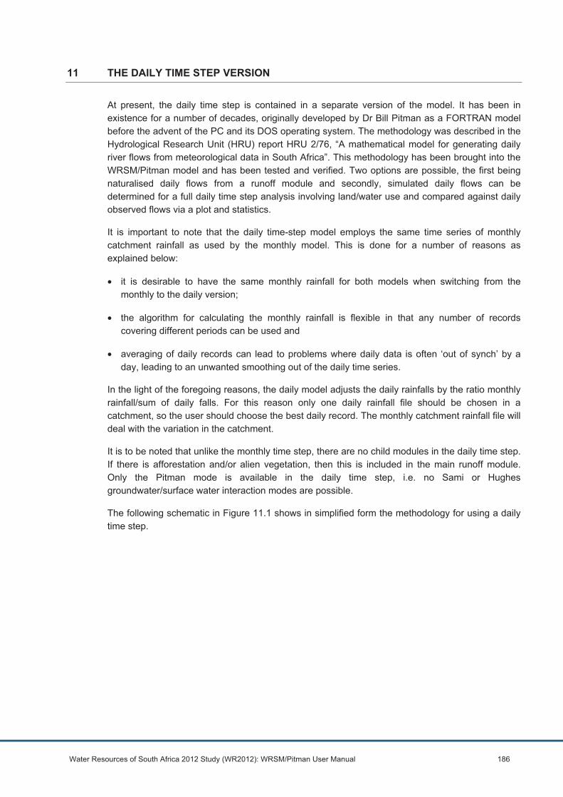
Water Resources of South Africa 2012 Study (WR2012): WRSM/Pitman User Manual 186
11 THE DAILY TIME STEP VERSION
At present, the daily time step is contained in a separate version of the model. It has been in existence for a number of decades, originally developed by Dr Bill Pitman as a FORTRAN model before the advent of the PC and its DOS operating system. The methodology was described in the Hydrological Research Unit (HRU) report HRU 2/76, “A mathematical model for generating daily river flows from meteorological data in South Africa”. This methodology has been brought into the WRSM/Pitman model and has been tested and verified. Two options are possible, the first being naturalised daily flows from a runoff module and secondly, simulated daily flows can be determined for a full daily time step analysis involving land/water use and compared against daily observed flows via a plot and statistics.
It is important to note that the daily time-step model employs the same time series of monthly catchment rainfall as used by the monthly model. This is done for a number of reasons as explained below:
• it is desirable to have the same monthly rainfall for both models when switching from the monthly to the daily version;
• the algorithm for calculating the monthly rainfall is flexible in that any number of records covering different periods can be used and
• averaging of daily records can lead to problems where daily data is often ‘out of synch’ by a day, leading to an unwanted smoothing out of the daily time series.
In the light of the foregoing reasons, the daily model adjusts the daily rainfalls by the ratio monthly rainfall/sum of daily falls. For this reason only one daily rainfall file should be chosen in a catchment, so the user should choose the best daily record. The monthly catchment rainfall file will deal with the variation in the catchment.
It is to be noted that unlike the monthly time step, there are no child modules in the daily time step. If there is afforestation and/or alien vegetation, then this is included in the main runoff module. Only the Pitman mode is available in the daily time step, i.e. no Sami or Hughes groundwater/surface water interaction modes are possible.
The following schematic in Figure 11.1 shows in simplified form the methodology for using a daily time step.

Wat
er R
esou
rces
of S
outh
Afri
ca 2
012
Stu
dy (W
R20
12):
WR
SM
/Pitm
an U
ser M
anua
l 18
7
Figu
re 1
1.1:
Flo
wch
art o
f dai
ly ti
me
step
pro
cess

Water Resources of South Africa 2012 Study (WR2012): WRSM/Pitman User Manual 188
The general components common to both methods will be dealt with first followed by the naturalised daily flow option and then the simulated daily flows including land use.
The main new components are as follows:
11.1 Edit menu – Network module
There is a daily time step tickbox (as shown in Figure 11.2 below) which now indicates whether the daily time step should be used. Also required are the daily simulation start and end years which must be contained within the monthly time step start and end years (typically they would be the same). Once a daily time step network is saved, a 1 will be entered on the last line of the network text file indicating a daily time step analysis.
Figure 11.2: The Daily Time Step Network
Once this network is loaded, a message on the screen will indicate that the daily time step version is being run.
11.2 Edit menu – Runoff module
The runoff module has an additional property tab called “Daily T/S Calibration” for calibration of daily parameters as shown in Figure 11.3. (T/S stands for Time Step.)
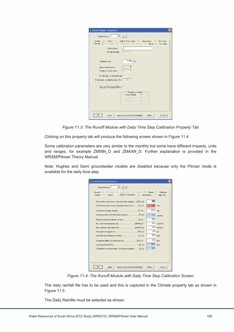
Water Resources of South Africa 2012 Study (WR2012): WRSM/Pitman User Manual 189
Figure 11.3: The Runoff Module with Daily Time Step Calibration Property Tab
Clicking on this property tab will produce the following screen shown in Figure 11.4
Some calibration parameters are very similar to the monthly but some have different impacts, units and ranges, for example ZMINN_D and ZMAXN_D. Further explanation is provided in the WRSM/Pitman Theory Manual.
Note: Hughes and Sami groundwater models are disabled because only the Pitman mode is available for the daily time step.
Figure 11.4: The Runoff Module with Daily Time Step Calibration Screen
The daily rainfall file has to be used and this is captured in the Climate property tab as shown in Figure 11.5 .
The Daily Rainfile must be selected as shown.

Water Resources of South Africa 2012 Study (WR2012): WRSM/Pitman User Manual 190
The format of the Daily Rainfile is very specific. An example is given below. The format is a 9 digit code, a space, the year, a space, the month, a space, the daily rainfall allowing for 4 digits (in tenths of a mm) and so on for the 31 values. In months with 28, 9 or 30 days a 0 is inserted. If there is no rain a +0 is inserted.

Wat
er R
esou
rces
of S
outh
Afri
ca 2
012
Stu
dy (W
R20
12):
WR
SM
/Pitm
an U
ser M
anua
l 19
1
Dai
ly R
ainf
all F
orm
at
299419 W
1959 1
75
85
1
128 29
165 130 380 +0
17
+0
+0
42
+0
+0
1
3
+0
+0
45
2
107 124 6
24
23
40
+0
284 3
7
299419 W
1959 2
+0
165 105 153 22
20
24
4
134 2
30
3
+0
86
350 255 195 3
+0
160 4
6
+0
+0
+0
8
30
28
+0
+0
+0
299419 W
1959 3
2
364 115 42
151 37
199 +0
85
130 53
+0
+0
350 10
24
11
75
12
+0
+0
+0
+0
+0
+0
+0
6
+0
+0
2
+0
299419 W
1959 4
+0
+0
+0
+0
+0
+0
+0
+0
+0
+0
36
+0
+0
+0
+0
+0
+0
+0
14
+0
195 145 34
+0
4
4
+0
55
448 +0
+0
299419 W
1959 5
+0
+0
245 +0
+0
+0
+0
+0
+0
1
29
215 +0
+0
75
195 415 7
+0
+0
+0
+0
+0
+0
+0
+0
+0
+0
+0
+0
+0
299419 W
1959 6
+0
+0
14
+0
+0
+0
+0
+0
+0
+0
+0
+0
+0
+0
+0
+0
+0
+0
+0
+0
+0
+0
+0
90
+0
+0
+0
+0
+0
+0
+0
299419 W
1959 7
+0
+0
+0
+0
+0
+0
+0
180 +0
+0
+0
+0
150 +0
+0
+0
80
+0
+0
+0
+0
+0
+0
+0
+0
+0
+0
+0
+0
+0
+0
299419 W
1959 8
+0
+0
+0
+0
+0
+0
20
+0
+0
+0
+0
+0
+0
+0
+0
1
+0
+0
+0
+0
+0
+0
+0
+0
+0
+0
+0
+0
+0
68
57
299419 W
1959 9
+0
+0
+0
+0
+0
+0
+0
+0
20
4
+0
56
84
+0
+0
+0
+0
+0
+0
+0
+0
1
+0
+0
+0
2
+0
+0
+0
2
+0
299419 W
1959 10
+0
+0
+0
+0
+0
+0
+0
10
137 100 +0
+0
+0
+0
+0
+0
+0
154 293 140 44
60
280 11
1
+0
237 +0
50
4
+0
299419 W
1959 11
85
55
1
+0
2
125 71
409 5
62
13
25
+0
65
7
295 113 58
77
+0
+0
25
+0
20
115 +0
23
13
+0
20
+0
299419 W
1959 12
4
219 27
6
20
50
11
+0
78
73
150 106 +0
+0
+0
180 275 290 155 +0
11
235 44
64
+0
3
+0
55
2
480
18

Water Resources of South Africa 2012 Study (WR2012): WRSM/Pitman User Manual 192
A conversion option has been provided in the File menu both for daily rainfall and daily observed streamflow. The daily rainfall input file allowed for is the SAWS daily rainfall of one day per line. The header rows must be deleted and the first date must be the 1st of October for a particular year as there needs to be a link with monthly and the first hydrological month is October. Up to 90 years of daily rainfall is allowed. The data should end on the 30th September of a particular year. Missing data should be patched. An example is given below.
There is a station number consisting of 7 digits, then a space and then another 1 digit number. Then the year, month and day as shown and finally the rainfall in tenths of a mm.
Note: The spaces must be exactly as shown below, i.e. 1 space, four spaces and 8 spaces between the values as shown below.
0636695 2 20131001 9.0 0636695 2 20131002 0.0 0636695 2 20131003 0.0 0636695 2 20131004 15.0 0636695 2 20131005 4.8
etc.
Figure 11.5 shows the File screen with “Select Daily Rainfall File to Convert” and “Select Converted Rainfall Output Filename” windows. Once these are selected, the “Convert to New Daily Rainfile” can be activated which will create the required file in WRSM/Pitman format.
Figure 11.5: Create a Daily Land Use File and Daily Flow Conversions screen
The output is shown on the next page. Leap years and non-leap years are taken into account.

Wat
er R
esou
rces
of S
outh
Afri
ca 2
012
Stu
dy (W
R20
12):
WR
SM
/Pitm
an U
ser M
anua
l 19
3
Non
-leap
yea
r
0636695 W 201310
90
0 0 150
48 2 184 6 0 0 0
20 0 0 0 2
0 0
0 114 2 0
38
38 0 0
0
0
0
0
10
0636695 W 201311
6
10 0 10
2 0 0 0 0 0 0
0 0 0 0 0
12 2
12 0 2 0
0
0 8 6
26
0
0
20
0
0636695 W 201312
90
0 0 250
48 2 284 6 0 0 0
20 0 0 0 2
0 0
0 214 2 0
38
38 0 0
0
0
0
0
30
0636695 W 201401
90
0 0 350
48 2 384 6 0 0 0
20 0 0 0 2
0 0
0 314 2 0
38
38 0 0
0
0
0
20
40
0636695 W 201402
90
0 0 450
48 2 484 6 0 0 0
20 0 0 0 2
0 0
0 414 2 0
38
38 0 0
0
50
0
0
0
0636695 W 201403
90
0 0 550
48 2 584 6 0 0 0
20 0 0 0 2
0 0
0 514 2 0
38
38 0 0
0
0
0
0
60
Leap
Yea
r
0636695 W 201110
90
0 0 150
48 2 184 6 0 0 0
20 0 0 0 2
0 0
0 114 2 0
38
38 0 0
0
0
0
0
10
0636695 W 201111
6
10 0 10
2 0 0 0 0 0 0
0 0 0 0 0
12 2
12 0 2 0
0
0 8 6
26
0
0
20
0
0636695 W 201112
90
0 0 250
48 2 284 6 0 0 0
20 0 0 0 2
0 0
0 214 2 0
38
38 0 0
0
0
0
0
30
0636695 W 201201
90
0 0 350
48 2 384 6 0 0 0
20 0 0 0 2
0 0
0 314 2 0
38
38 0 0
0
0
0
0
40
0636695 W 201202
90
0 0 450
48 2 484 6 0 0 0
20 0 0 0 2
0 0
0 414 2 0
38
38 0 0
0
0
50
0
0
0636695 W 201203
90
0 0 550
48 2 584 6 0 0 0
20 0 0 0 2
0 0
0 514 2 0
38
38 0 0
0
0
50
0
60

Water Resources of South Africa 2012 Study (WR2012): WRSM/Pitman User Manual 194
For the daily observed streamflow file conversion, the DWS input of one line per day has been allowed for as shown in the following example. As with the rainfall data, the header lines and data up to 1st October must be deleted, i.e. the first row must be the 1st of October for any particular year. The data should end on the 30th September of a particular year to tie up with the hydrological year. Up to 50 years of daily data is allowed,.
Note: The spaces must be exactly as shown below, i.e. 5 spaces and 5 spaces between the values as shown below.
19531001 0.010 2 19531002 0.020 2 19531003 0.030 2 19531004 0.040 2 19531005 0.050 2 19531006 0.060 2
The tool for this is to be found in the File drop down menu system as shown in Figure 11.5 . Firstly the “Select a Daily Obs Flow File to Convert” box is chosen and using the button with three dots, the daily observed flow file is selected from a folder. Then a file can either be selected or typed in in the box next to “Select Converted Observed Flow Output Filename”. Finally the “Convert to new Daily Obs Flow File” button is pressed and the new daily file in WRSM/Pitman model format is determined. Up to 70 years of daily flow data can be dealt with (otherwise do in two conversions).
There is the year, month and day then the daily observed streamflow in cubic metres per second and finally a code indicating the quality of the data. A -1.00 is used if the day does not exist in a month. NB. Missing data must preferably be patched or have a 0.00 entered otherwise the code will be read as the value since free format is used. No “+” symbol must be entered after the 0.00 as with 2 decimal places allowed for and data which can exceed 999 cumecs, the full seven space field is required. Following transformation using the program the data will look as follows:

Wat
er R
esou
rces
of S
outh
Afri
ca 2
012
Stu
dy (W
R20
12):
WR
SM
/Pitm
an U
ser M
anua
l 19
5
Non
-leap
yea
r
1953
10
0.01
0.02
0.03
0.04
0.05
0.06
0.07
0.08
0.09
0.10
0.11
0.12
0.13
0.14
0.15
0.16
0.17
0.18
0.19
0.20
0.21
0.22
0.23
0.24
0.25
0.26
0.27
0.28
0.29
0.30
0.31
1953
11
0.01
0.02
0.03
0.04
0.05
0.06
0.07
0.08
0.09
0.10
0.11
0.12
0.13
0.14
0.15
0.16
0.17
0.18
0.19
0.20
0.21
0.22
0.23
0.24
0.25
0.26
0.27
0.28
0.29
0.30
-1.0
1953
12
0.01
0.02
0.03
0.04
0.05
0.06
0.07
0.08
0.09
0.10
0.11
0.12
0.13
0.14
0.15
0.16
0.17
0.18
0.19
0.20
0.21
0.22
0.23
0.24
0.25
0.26
0.27
0.28
0.29
0.30
0.31
1954
01
0.01
0.02
0.03
0.04
0.05
0.06
0.07
0.08
0.09
0.10
0.11
0.12
0.13
0.14
0.15
0.16
0.17
0.18
0.19
0.20
0.21
0.22
0.23
0.24
0.25
0.26
0.27
0.28
0.29
0.30
0.31
1954
02
0.01
0.02
0.03
0.04
0.05
0.06
0.07
0.08
0.09
0.10
0.11
0.12
0.13
0.14
0.15
0.16
0.17
0.18
0.19
0.20
0.21
0.22
0.23
0.24
0.25
0.26
0.27
0.28
-1.0
-1.0
-1.0
1954
03
0.01
0.02
0.03
0.04
0.05
0.06
0.07
0.08
0.09
0.10
0.11
0.12
0.13
0.14
0.15
0.16
0.17
0.18
0.19
0.20
0.21
0.22
0.23
0.24
0.25
0.26
0.27
0.28
0.29
0.30
0.31
Leap
yea
r
1953
10
0.01
0.02
0.03
0.04
0.05
0.06
0.07
0.08
0.09
0.10
0.11
0.12
0.13
0.14
0.15
0.16
0.17
0.18
0.19
0.20
0.21
0.22
0.23
0.24
0.25
0.26
0.27
0.28
0.29
0.30
0.31
1953
11
0.01
0.02
0.03
0.04
0.05
0.06
0.07
0.08
0.09
0.10
0.11
0.12
0.13
0.14
0.15
0.16
0.17
0.18
0.19
0.20
0.21
0.22
0.23
0.24
0.25
0.26
0.27
0.28
0.29
0.30
-1.0
1953
12
0.01
0.02
0.03
0.04
0.05
0.06
0.07
0.08
0.09
0.10
0.11
0.12
0.13
0.14
0.15
0.16
0.17
0.18
0.19
0.20
0.21
0.22
0.23
0.24
0.25
0.26
0.27
0.28
0.29
0.30
0.31
1954
01
0.01
0.02
0.03
0.04
0.05
0.06
0.07
0.08
0.09
0.10
0.11
0.12
0.13
0.14
0.15
0.16
0.17
0.18
0.19
0.20
0.21
0.22
0.23
0.24
0.25
0.26
0.27
0.28
0.29
0.30
0.31
1954
02
0.01
0.02
0.03
0.04
0.05
0.06
0.07
0.08
0.09
0.10
0.11
0.12
0.13
0.14
0.15
0.16
0.17
0.18
0.19
0.20
0.21
0.22
0.23
0.24
0.25
0.26
0.27
0.28
0.29
-1.0
-1.0
1954
03
0.01
0.02
0.03
0.04
0.05
0.06
0.07
0.08
0.09
0.10
0.11
0.12
0.13
0.14
0.15
0.16
0.17
0.18
0.19
0.20
0.21
0.22
0.23
0.24
0.25
0.26
0.27
0.28
0.29
0.30
0.31
.
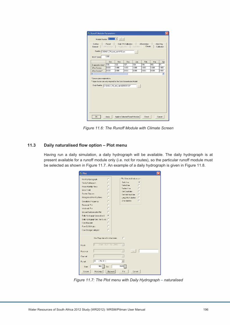
Water Resources of South Africa 2012 Study (WR2012): WRSM/Pitman User Manual 196
Figure 11.6: The Runoff Module with Climate Screen
11.3 Daily naturalised flow option – Plot menu
Having run a daily simulation, a daily hydrograph will be available. The daily hydrograph is at present available for a runoff module only (i.e. not for routes), so the particular runoff module must be selected as shown in Figure 11.7. An example of a daily hydrograph is given in Figure 11.8.
Figure 11.7: The Plot menu with Daily Hydrograph – naturalised
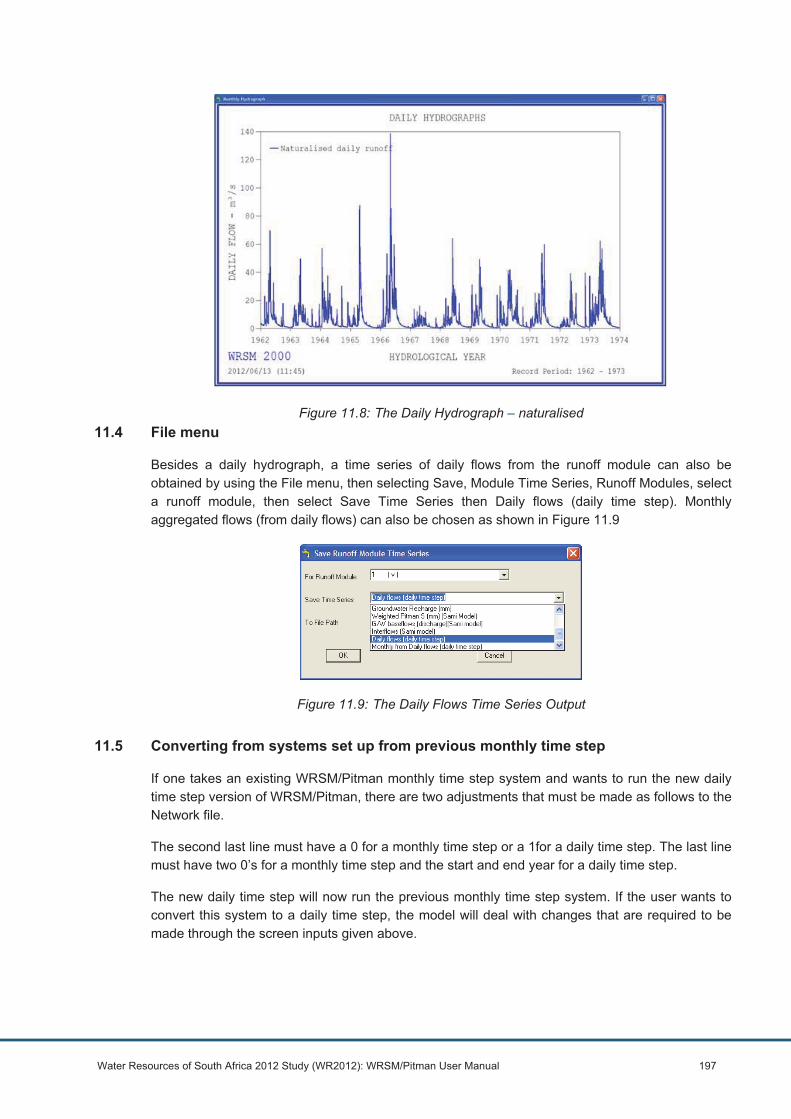
Water Resources of South Africa 2012 Study (WR2012): WRSM/Pitman User Manual 197
Figure 11.8: The Daily Hydrograph – naturalised 11.4 File menu
Besides a daily hydrograph, a time series of daily flows from the runoff module can also be obtained by using the File menu, then selecting Save, Module Time Series, Runoff Modules, select a runoff module, then select Save Time Series then Daily flows (daily time step). Monthly aggregated flows (from daily flows) can also be chosen as shown in Figure 11.9
Figure 11.9: The Daily Flows Time Series Output
11.5 Converting from systems set up from previous monthly time step
If one takes an existing WRSM/Pitman monthly time step system and wants to run the new daily time step version of WRSM/Pitman, there are two adjustments that must be made as follows to the Network file.
The second last line must have a 0 for a monthly time step or a 1for a daily time step. The last line must have two 0’s for a monthly time step and the start and end year for a daily time step.
The new daily time step will now run the previous monthly time step system. If the user wants to convert this system to a daily time step, the model will deal with changes that are required to be made through the screen inputs given above.

Water Resources of South Africa 2012 Study (WR2012): WRSM/Pitman User Manual 198
11.6 Daily simulated flow option including land use
Having established the naturalized daily flows from runoff modules methodology, the natural extension of this was to include the effects of land use and be able to compare simulated and observed daily flows anywhere in a WRSM/PITMANnetwork. This issue has been discussed in meetings and debated between the following persons with experience in water resources modelling and model development:
• Dr Bill Pitman; • Mr Allan Bailey; • Dr Chris Herold and • Mr Grant Nyland.
Land use involves irrigation, afforestation, alien vegetation, wetlands, reservoirs, paved surfaces, mining, abstractions, return flows and also involves the groundwater/surface water interaction. Methodologies have been developed for all these by a number of different experts such as Dr Bill Pitman, Prof. Denis Hughes, Dr David le Maitre, Dr David Scott, Dr Chris Herold, Trevor Coleman and Karim Sami and are all based on a monthly time step. It is worth noting at this stage that daily data is exceedingly difficult to obtain for land use, in fact it is generally very difficult to obtain even on a monthly time step. It has also been widely reported in the last year that rainfall and observed streamflow data is declining and graphs have been developed showing the alarming drop off in rainfall stations and observed streamflow sites that for which even monthly data is available.
Bearing all this in mind, it was therefore decided to provide a practical and simplified method to analyse simulated flows and include land use. The methodology is as follows and involves use of the monthly and daily time step versions:
Monthly time step version
• Firstly the monthly time step is used and the streamflow gauge in question is calibrated and
• The monthly naturalised streamflow and simulated streamflow is then determined as usual for this route where the streamflow gauge is situated;
Daily Time Step version
• The daily time step is now used and naturalized daily flows are determined for all runoff modules upstream of the streamflow gauge in question. Save the naturalised daily flow files under File| Save| Module Time Series| Runoff Modules| Daily Flows daily time step| Choose a runoff module and Save Time Series. This creates files of the form (for example) “SCRRU1dfl.mts” where SCR is an example of the network name and 1 is an example of a runoff module number;
• Now go to File| Create a Daily Land Use File and Daily File Conversions;
• Enter the two output file names in the first two blocks (any names you like) for “Daily Land Use Flow Output File” and “Daily Simulated Output File”;
• Enter the two input file names for the third and fourth blocks that you determined from the monthly time step (step 2);

Water Resources of South Africa 2012 Study (WR2012): WRSM/Pitman User Manual 199
• A daily land use file is determined by taking the monthly NAT-SIM and dividing by the number of days in the month. The button: “Calculate monthly and daily land use flow files” does this for you and the “Daily Land Use Flow Output File” is created;
• Then the button “Naturalised Daily Flow Files” together with “Add” sets up the “Naturalised Daily Flow Files to Add” window and gives the total naturalised flow at the route in question, i.e. you add up all the (for example) SCRRU1dfl.mts files;
• The total naturalised daily flows then have the daily land use file subtracted (the button “Calculate simulated daily flow file” does this) so it needs the total of the naturalised daily flow files and the “Daily Land Use Flow Output File” determined before to create the “Daily Simulated Output File”
• Now in Plot, the daily observed file that you determined separately and converted to the right format using the “Convert to new OBS flow file” button at this streamflow gauge is entered. The “Daily simulated Output flow file” (determined after step 8) is also entered;
• The graph of simulated daily and observed flows can then be plotted by selecting the route, checking on the start and end years and pressing the Screen button;
• The fit between simulated and observed flows can be improved by calibration of the daily calibration parameters and then repeating steps 4, 5 and 7. Dr Bill Pitman has provided the following advice in Table 11.1 on converting from monthly calibration parameters to daily calibration parameters.
Table 11.1: Conversion from monthly to daily calibration parameters
Calibration Parameter Monthly Daily Dr Bill Pitman’s Rule
POW 2 2 No difference
SL 0 0 Usually = 0
ST 160 160 No difference
FT 20 0.3 FT (Daily) = 0.024 of monthly (=0.48)
AI 0
Zmin 999 0 None (range 0-3 for daily)
Zmax 999 15 None (range 6-15 for daily)
PI 1.5 1.5
TL 0.25 5 TL (daily) = 1 + 0.00025 * Area (km²) * TL (monthly model – months) / 0.25 =
Lag 0
GL 10 GL (daily model – days) = 25 * GL (monthly model – months) (If Pitman method used otherwise default value)
R 0.5 0.5 No difference
Testing has been carried out on the Olifants Water Management Area (WMA) on tertiary catchment B42 and the comparison was good (refer to Figure 11.10).
Of all the various land use types, irrigation is most affected by rainfall, i.e. the first part of the month may be very dry and the farmer will irrigate and then there could be a large rainfall event in the latter part of the month and the farmer will stop irrigating. For this reason, if there is large scale irrigation in a catchment and/or the catchment is very small, dividing the combined effect of land

Water Resources of South Africa 2012 Study (WR2012): WRSM/Pitman User Manual 200
use by the number of days in the month could provide results that are a bit coarse. However, for large scale catchments and/or catchments where irrigation is not a major component, the above methodology is regarded as applicable.
The methodology described for comparing daily simulated and observed flows above has been streamlined in WRSM/PITMAN to make it relatively easy for the user to analyse. Accordingly the following new screens have been developed:
• Under the File Menu – Create a Daily Land Use File. This menu prompts the user for required output file names, monthly and daily files and performs the necessary file manipulations using two Calculate buttons.
Figure 11.10: Determining a daily simulated flow file (including land use)
• Having developed the required files outlined in Figure 11.10, the Plot menu is then accessed to compare simulated and observed daily flows. This menu has been expanded as shown in Figure 11.10. Note that there are two options in this menu for daily flows, i.e. naturalized daily flows from a runoff module and simulated daily flows including land use.
Figure 11.11: The Plot menu with Daily Simulated Hydrograph – including land use

Water Resources of South Africa 2012 Study (WR2012): WRSM/Pitman User Manual 201
Following this methodology will culminate in a graph shown in Figure 11.12.
Figure 11.12: The Daily Simulated versus Observed Hydrograph – including land use
Water Resources of South Africa 2012 Study (WR2012): WRSM/Pitman User Manual 202
REFERENCES
1. Pitman WV (1973). A Mathematical Model for Generating Monthly River Flow from Hydro Meteorological Data in South Africa. Hydrological Research Unit Report No. 2/73, University of the Witwatersrand, Johannesburg.
2. Midgley DC, Pitman WV & Middleton BT (1981). Surface Water Resources of South Africa – Volumes I to VI. Hydrological Research Unit Report Nos. 8/81 to 13/81, University of the Witwatersrand, Johannesburg.
3. Pitman WV & Kakebeeke JP (1991). Water Resources Simulation Model, Stewart Scott (formerly Stewart, Sviridov & Oliver).
4. Pitman WV, Kakebeeke JP and Bailey AK (2001). WRSM2000. Water Resources Simulation Model for Windows User’s Guide. September 2000.
5. Midgley DC, Pitman WV & Middleton BJ (1990). Surface Water Resources of South Africa 1990 – Volumes I to VI. Water Resources 1990 Joint Venture – Steffen, Robertson and Kirsten Inc/ Stewart Scott Inc/ Knight Piesold Inc (formerly Watermeyer, Legge, Piesold and Uhlmann)
6. Sami K, (2005). Technical Documentation for Surface – Groundwater Interaction use in System Models: Task 3b
7. Hughes D.A., Parsons R. Ground Water Pitman Model Version 3 – Model Description and Calibration.
8. DF Scott and RE Smith (1997) – “Preliminary empirical models to predict reductions in total and low flows resulting from afforestation“ in Water SA Vol 23 No. 2 April 1997
9. D le Maitre and A Görgens (2001) “Invasive Alien Vegetation and Dam Yields – Illustrating the Impact of Clearing Programmes on Assurance of Supply“ – Draft report to WRC February 2001.
10. Allen, (1988) – Water Quality Modelling Volume A: Water Quality Calibration Model by RB Allen and Dr C Herold DWA Report Number PC000/00/7086 of March, 1988.
11. WRSM2000 Theory (Stewart Scott, 2006)

Water Resources of South Africa 2012 Study (WR2012): WRSM/Pitman User Manual 203
APPENDIX A: GRAPH MANUAL
A1. Plot
This portion of the manual describes the Plot functionality in the WRSM/Pitman application. The plot functionality is only active after running the simulation. The plot functionality is activated from the menu by selecting the “Plot” menu option or by clicking on the “Plot” speed button:
Figure A.1: Menu Options
The Plot menu option or button will launch the “Plot” dialog:
Figure A.2: Plot Menu
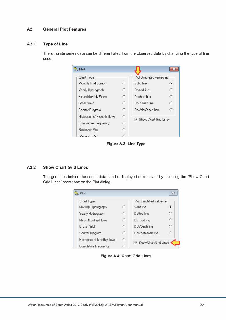
Water Resources of South Africa 2012 Study (WR2012): WRSM/Pitman User Manual 204
A2 General Plot Features
A2.1 Type of Line
The simulate series data can be differentiated from the observed data by changing the type of line used.
Figure A.3: Line Type
A2.2 Show Chart Grid Lines
The grid lines behind the series data can be displayed or removed by selecting the “Show Chart Grid Lines” check box on the Plot dialog.
Figure A.4: Chart Grid Lines

Water Resources of South Africa 2012 Study (WR2012): WRSM/Pitman User Manual 205
A2.3 General Features of the Plots
Figure A.5: General Plot Features
A2.3.1 General
• The Y axis will change its scale between linear and logarithmic when it is clicked on.
• The maximum value of the Y axis will adjust if the mouse wheel is rotated while the mouse is over the chart.
• A ‘Back’ button is provided to close the plot window and return to the Plot dialog.
• The graph ‘remembers’ its screen position from one display to the next.
• A single point in the time series (not having any points either side of it) is shown as a little circle. A discontinuity in the time series is shown as a gap in the line.
A2.3.2 Zooming
• The graph can be zoomed with the mouse. Click with the left button at the top of the area that is required to be viewed. Drag the mouse curser down to the bottom and left. Let the left button go and the charts will zoom to the selected area.
• Click on the bottom left and drag towards the top right. The graph will ‘un-zoom’ when the left button is released. The graph returns to view the full data set.
• Fixed zoom span buttons are provided to view a specific popular time span – ten years, 50 years, etc.
• Buttons are provided to enter a specific start date and end date.
• Simple zoom-in and zoom-out buttons are also provided.

Water Resources of South Africa 2012 Study (WR2012): WRSM/Pitman User Manual 206
A2.3.3 Panning
• A number of panning buttons are provided to move the visible data to the left or the right without changing the zoom resolution.
• The double arrows ‘<<’ and ‘>>’ pan a page to the left or right – exactly the current screen width. For example, if a ten year span is being viewed, these buttons will shift the view exactly ten years to the left or right.
• The single arrows ‘<’ and ‘>’ nudge the view a small amount to the left or right.
• One can hold the right button down and drag the graph with the mouse.
A2.3.4 Printing
• A “Print” button is provided to produce a quick printout of the current graph. A print preview is displayed using Internet Explorer which provides standard printing capability for the user’s computer.
• The elements in the report like the chart pictures can be selected with the mouse and copied to the clip-board. These can then be pasted directly into many Windows programs.
• A number of files are created when the Print button is selected.
o Each chart is saved as a ‘*.emf’ in the same directory as the application. These can be imported into most presentation and reporting packages.
o Many of the elements of these pictures can be modified or removed. New annotations can also be added.
o A file called ‘Report.htm’ is also created. This file can be opened with a word processing package like MS Word. The resulting Word document will look exactly like the report.
o The report can also be imported directly into an existing report. In MS Word for example, select the menu option “Insert” – “File…” and select the ‘Report.htm’ file.
• A “Data” button is provided to access the raw data contained in the current view. A print preview is displayed using Internet Explorer which allows the data to be accessed.
• Single data values or entire data blocks can be selected and copied to the clip-board. This data can then be pasted directly into a spreadsheet program like MS Excel. Each data value will be placed in its own cell when pasting.
• The data file is also written to disk as “ReportData.htm”. This file can be opened directly with MS Excel and each data value will be placed in its own cell.
• The data file can also be inserted directly into an existing report in the same way as described for the report above.
