X-Ray Emissions from Charge Exchange in the Heliosphere

Ina P. Robertson1, Thomas E. Cravens1, Mikhail V. Medvedev1, and Timur Linde2

1Department of Physics and Astronomy, University of Kansas, Lawrence, KS 66045, USA 2University of Chicago, Department of Astronomy and Astrophysics, Chicago, IL 60637, USA

Abstract. X-Rays are generated throughout the heliosphere and the terrestrial magnetosheath as a consequence of charge transfer between heavy solar wind ions and interstellar and geocoronal neutrals. These X-ray intensities, as observed from Earth, depend on look direction and season. Due to rapid variation in geocoronal X-ray emissions in response to time variations in the solar wind flux, it might very well be possible to observe Earth’s magnetosheath from an observation point outside the geocorona. In previous papers we have shown that there is significant correlation between “long term enhancements” in the soft X-ray background measured by the Röntgen Satellite (ROSAT), and that roughly 25-50% of the Soft X-ray background maps are of heliospheric origin. In this paper we present a preliminary simulated soft X-ray image of the heliosphere as would be seen by an external observer.

INTRODUCTION

In 1996 X-ray emission from the comet Hyakutake was discovered [1]. Cravens [2] proposed that this emission could be explained by charge exchange collisions between heavy solar wind ions and cometary neutrals (SWCX). In this charge exchange the product ion is left in an excited state and eventually emits a photon in the X-ray or EUV region of the spectrum [3]. Cox [4] suggested that this same process could be applied to interaction between solar wind ions and interstellar neutrals and neutrals in Earth’s geocorona and might be able to explain some of the temporal variation in the observed soft X-ray background (SXRB). Dennerl et al. [5] suggested that this charge exchange mechanism might be able to explain the Long Term Enhancement (LTE) part of the SXRB. Cravens [6] created a simple model of the heliospheric x-ray emissions and concluded that about half of the SXRB could be explained by this mechanism. A significant correlation between measured solar wind proton fluxes and measured LTE X-ray intensities was also found [7, 8]. Robertson and Cravens [8] constructed maps of predicted heliospheric X-rays as seen from Earth. They also studied SWCX X-rays associated with geocoronal neutral hydrogen [9]. Due to an increase in solar wind density and temperature, there was a significant enhancement of X-ray intensities in the subsolar point region, clearly showing the bow shock and the magnetopause. They concluded that it is possible to remotely image the solar wind flow around the magnetosphere.

In the current paper we will present a simulated soft X-ray image of the heliosphere as seen from the outside. Predicting X-ray production from the SWCX mechanism requires knowledge of the distribution of the solar wind and interstellar neutrals throughout the region. An increase in solar wind density takes place at the termination shock where the solar wind becomes sub-sonic and hot. As the solar wind approaches the heliopause, it diverts and proceeds to flow toward the tail region of the heliopause [10]. This region is called the heliosheath. In particular in the nose region of the heliosheath, the solar wind density increases and the total velocity, which now includes a large thermal component, increases too.

Interstellar neutral hydrogen can flow into the heliosphere, but it interacts with plasma weakly at the heliopause [11]. This creates an abundance of hydrogen in the region between the heliopause and the outer bow shock called the hydrogen wall. Some of the higher hydrogen densities, however, can be noticed within the heliopause where a relatively high density solar wind exists. We expect an enhanced X-ray production in this region.

THE CHARGE EXCHANGE MODEL

Charge exchange between solar heavy ions and interstellar/geocoronal neutrals can be depicted as follows:

+++

+!+ MOMO*67 (1)

where O7+ is an example of a heavy solar wind ion and M represents an interstellar or geocoronal neutral atom. The star indicates that O6+ is in an excited state. The excited O6+ ion emits a photon with energy in the extreme ultra-violet or soft X-ray region.

To model the volume power production of this charge exchange, the following equation is used:

( )13 !!

! = seVcmunnP swnswrayX " (2) The factor α is an efficiency factor for the entire soft X-ray part of the spectrum and

is proportional to the relative of abundance of heavy solar wind ions in the solar wind and also the average charge transfer cross sections for high charge state ions. The factor α should be different for each neutral target as well as for different composition states of the solar wind [12]. This factor can also only be used for the colissionally thin case. nsw, usw and nn are the solar wind proton density, the solar wind speed and the neutral atom density respectively.

The solar wind is considered to flow out radially within the termination shock. Its velocity is mainly bulk velocity, which is an average of 400 km/s at lower latitudes and 700-800 km/s at high latitudes. The difference in velocities is the main reason for the elongation of the termination shock in the polar direction. As the solar wind passes the termination shock, the solar wind, however, slows down and heats up. Although the bulk velocity reduces, the thermal velocity now becomes a significant contributor

to the

total velocity. The solar wind cannot pass the heliopause and is diverted tailward.

FIGURE 1. Production Rates of SWCX with neutral interstellar hydrogen

Interstellar hydrogen interacts weakly with plasma near the heliopause, where it

slows down and heats up. It then enters the heliopause and as it travels through the heliopause it is depleted due to photo-ionization and charge exchange reactions [13]. Radiation pressure causes a depletion cavity near the sun. The hydrogen density is larger in the upwind than in the downwind direction. Even though the solar wind flux varies with time, X-ray emissions due to SWCX with interstellar hydrogen vary little over time due to the averaging effects of long optical paths [6].

Interstellar neutral helium does not experience stagnation upon entering the heliosphere. Its density is about an order of magnitude less than that of interstellar hydrogen. Neutral helium can get closer to the sun and experiences a gravitational force, which causes the interstellar helium to focus behind the sun, giving rise to the helium cone which shows a dramatic increase in density compared to the upwind density. Look direction, therefore, is important for SWCX X-rays. In the upwind direction there will be a higher soft X-ray intensity due to SWCX with interstellar hydrogen, and less due to SWCX with interstellar helium; in the downwind direction, however, SWCX with interstellar helium dominates [8]. X-ray emissions due to SWCX with interstellar helium also reflect the time variation which is evident in the solar wind proton flux. This can also be said of SWCX with geocoronal neutral hydrogen [9]. Of the three types of charge exchange collisions, the greatest time variation is with geocoronal hydrogen.

Finally, in all observations from Earth, the greatest contributors to the X-ray intensities are exchanges taking place within the first 10 AU near the sun. However, for an X-ray observer outside the heliosphere structure in the outer heliosphere (for instance the termination shock) becomes interesting.

HELIOSPHERIC X-RAY EMISSIONS AS SEEN FROM EARTH

Figure 1 shows SWCX X-ray production rates along a line of sight from Earth directly into the interstellar wind direction. We used the solar wind density, speed and neutral hydrogen density from a three-dimensional model of the heliosphere [14]. At 80 AU the effect of the termination shock on the production rates is clearly evident, and at 110 AU we can see the effect of the beginning of the hydrogen wall. In previous publications [6,7,8] neither the increase in solar wind density at the termination shock nor the increase in hydrogen density at the heliopause was taken into account. The reason for this is that most of the contribution to the SWCX X-ray intensities as observed from Earth comes from charge exchange within about 10 AU from Earth. The increase in production rate at the termination shock and in the heliosheath only affects the total intensity by about 10%. What does affect Earth-centered observations of SWCX X-rays is season and look direction, as is evident in Robertson and Cravens 2003 maps [8].

EXTERNAL X-RAY VIEW OF THE HELIOSPHERE

If the heliosphere is observed from the outside, SWCX X-ray production at the termination shock and in the heliosheath is important. A simple model was created using simulated solar wind and interstellar neutral hydrogen parameters [14] which show the presence of the termination shock and hydrogen wall. Equation (2) was used to determine the production rate along 51 × 101 lines of sight. Since the solar wind temperature increases by about 2 orders of magnitude, the solar wind thermal velocity is taken into account in the production rate calculation.

Figure (2) shows one of the production rate plots that we generated. The plot is in the x-z plane with the z-axis going from South to North Pole in the solar ecliptic coordinate system. The x-axis is pointing near the interstellar wind direction, which is at 252° longitude. However, a 7 degree tilt with respect to the ecliptic plane was not taken into account.

In order to see structure inside the heliosphere, a maximum limit on the scale was set. This saturates the production rates generated near the heliopause. Also, the region from 0-40 AU is in black, because our solar wind and interstellar hydrogen generated data starts at 40 AU [14,15]. However this is the region where we find the largest production rates since the solar wind flux is at a maximum [8]. In reality we would

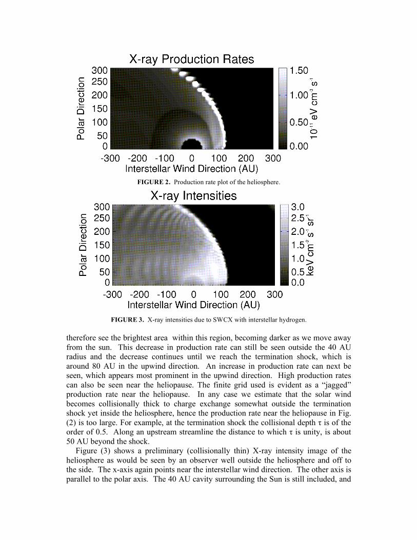
FIGURE 2. Production rate plot of the heliosphere.

FIGURE 3. X-ray intensities due to SWCX with interstellar hydrogen.

therefore see the brightest area within this region, becoming darker as we move away from the sun. This decrease in production rate can still be seen outside the 40 AU radius and the decrease continues until we reach the termination shock, which is around 80 AU in the upwind direction. An increase in production rate can next be seen, which appears most prominent in the upwind direction. High production rates can also be seen near the heliopause. The finite grid used is evident as a “jagged” production rate near the heliopause. In any case we estimate that the solar wind becomes collisionally thick to charge exchange somewhat outside the termination shock yet inside the heliosphere, hence the production rate near the heliopause in Fig. (2) is too large. For example, at the termination shock the collisional depth τ is of the order of 0.5. Along an upstream streamline the distance to which τ is unity, is about 50 AU beyond the shock.

Figure (3) shows a preliminary (collisionally thin) X-ray intensity image of the heliosphere as would be seen by an observer well outside the heliosphere and off to the side. The x-axis again points near the interstellar wind direction. The other axis is parallel to the polar axis. The 40 AU cavity surrounding the Sun is still included, and

can be seen in Fig. 3. This region would, in reality, show up as the brightest area. In order to see the structure inside the heliopause, the maximum intensity scale has been reduced, which causes saturation of the intensity near the heliopause. But the calculated intensity near the heliopause is too large anyway, due to collisional thickness effects. Nevertheless we can see the increase in X-ray intensities in the heliosheath region indicative of the increase in solar wind density, temperature and neutral hydrogen densities.

CONCLUSIONS

Wargelin and Drake [16] state that X-rays due to charge exchange between highly charge ions in stellar wind and interstellar neutrals might be detectable and could give us information about other stellar winds and their charge exchange with the interstellar neutral wind. Modeling our heliosphere can provide insights into how the interaction of hot stellar wind of other stars with their local interstellar medium might be detected and the morphology observed.

ACKNOWLEDGMENTS

This work was supported by NASA Planetary Atmospheres grant NAG5-11038 and NSF grant ATM-0234271 to the University of Kansas.

REFERENCES

1. Lisse, C.M., K. Dennerl, J. Englhauser, M. Harden, F.E. Marshall, M.J. Mumma, R. Petre, J.P. Pye, M.J. Ricketts, J. Schmitt, J. Trümper and R.G. West, Discoverey of X-ray and extreme ultraviolet emission from Comet C/Hyakutake 1996 B2, Science, 274, 205, (1996).

2. Cravens, T. E., Comet Hyakutake x-ray source: charge transfer of solar wind heavy ions, Geophys. Res. Lett., 24, 105, (1997).

3. Cravens, T. E., X-ray emission in the solar system, in Atomic Processes in Plasmas: 13th APS Topical Conference on Atomic Processes in Plasmas, edited by D.R. Schultz et al., AIP, Melville, NY, 2002, p. 173.

4. Cox, D. P., Modeling the local bubble, in The Local Bubble and Beyond, edited by D. Breitschwerdt, M. J. Freyberg, and J. Trümper, Springer-Verlag, New York, 1998, p. 121.

5. Dennerl, K., J. Englhauser, and J. Trümper, X-ray emissions from comets detected in the Röntgen X-ray satellite all-sky survey, Science, 277, 1625, (1997).

6. Cravens, T. E., Heliospheric x-ray emission associated with charge transfer of the solar wind with interstellar neutrals, Astrophys. J., 532, L153, (2000).

7. Cravens, T. E., I. P. Robertson, and S. L. Snowden, Temporal variations of geocoronal and heliospheric x-ray emission associated with the solar wind interaction with neutrals, J. Geophys. Res., 106, 24,883, (2001).

8. Robertson, I. P., and T. E. Cravens, Spatial maps of heliospheric and geocoronal X-ray intensities due to the charge exchange of the solar wind with neutrals, J. Geophys. Res., 108, A10, 8031, doi:10.1029/2003JA009873, 2003.

9. Robertson, I. P., and T. E. Cravens, X-Ray Emission from the Terrestrial Magnetosheath, Geophys. Res. Lett., 30 (8), 1439, doi:10.1029/2002GL016740, 2003.

10. Zank, G. P., Interaction of the solar wind with the local interstellar medium: a theoretical perspective, Space Science Reviews, 89, 431, (1999).

11. Frisch, P. C., The Local Bubble, Local Fluff, and Heliosphere, in The Local Bubble and Beyond, edited by D. Breitschwerdt, M. J. Freyberg, and J. Trümper, Springer-Verlag, New York, 1998, p. 269.

12. Schwadron, N. A., and T. E., Cravens, Cometary X-ray emission for slow and fast solar wind, Astrophys. J., 544, 558, 2000.

13. Chassefiere, E., Bertaux, J. L., Lallemant, R., and Kurt, V. G., Atomic hydrogen and helium densities of the interstellar medium measured in the vicinity of the sun, Astron. Astrophys., 160, 229, 1986.

14. Linde, T. J., A Three-Dimensional Adaptive Multifluid MHD Model of the Heliosphere, Ph.D. Thesis, 1998. 15. Linde, T. J., T. I. Gombosi, P. L. Roe, K. G. Powell, and D. L. DeZeeuw, Heliosphere in the Magnetized Local

Interstellar Medium: Results of a three-dimensional MHD Simulation, J. Geophys. Res., 103, 1889, (1998). 16. Wargelin, B. J., and J. J. Drake, Observability of Stellar Winds from Late-Type Dwarfs via Charge Exchange

X-Ray Emission, Astrophys. J., 546, L57-60, (2001).