,x ,x n/ - web services overviewweb.cecs.pdx.edu/~edam/slides/decisiontheoryx4.pdf · target vs....
TRANSCRIPT
Target vs. Sampled
• The target population and the sample population are usuallydifferent
• Difficult to collect unbiased samples
• Many studies are self selecting
• This is less of an issue for engineering problems
• Must be careful to collect “training” data and “test” data undersame conditions
J. McNames Portland State University ECE 4/557 Decision Theory Ver. 1.19 3
Statistical Decision Theory Overview
• Definitions
• Estimation
• Central Limit Theorem
• Test Properties
• Parametric Hypothesis Tests
• Examples
• Parametric vs. Nonparametric
• Nonparametric Tests
J. McNames Portland State University ECE 4/557 Decision Theory Ver. 1.19 1
What is a Point Statistic?
• A point statistic is a number computed from a random sample:X1, X2, . . . Xn
• It is also a random variable
• Example: Sample average
X =1n
n∑i=1
Xi
• Conveys a type of summary of the data
• Is a function of multiple random variables
• Specifically, a function that assigns real numbers to the points ofa sample space.
J. McNames Portland State University ECE 4/557 Decision Theory Ver. 1.19 4
Definitions
Experiment: process of following a well-defined procedure where theoutcome is not known prior to the experiment
Population: collection of all elements (N) under investigation.
Target Population: population about which information is wanted.
Sample Population: population to be sampled.
Sample: collection of some elements (n) of a population.
Random Sample: sample in which each element in the populationhas an equal probability of being selected in the sample.Alternatively, a sequence of independent and identicallydistributed (i.i.d.) random variables, X1, X2, . . . Xn.
Theoretically, random samples must be drawn with replacement.However, for large populations, there is little difference (n ≤ N/10)where n = size of sample and N = size of the sample population.
J. McNames Portland State University ECE 4/557 Decision Theory Ver. 1.19 2

Example 1: MATLAB Code
function [] = PrctilePlot();
FigureSet(1,’LTX’);
p = 0:0.1:100;
y = prctile(1:10,p);
h = plot(p,y);
set(h,’LineWidth’,1.5);
xlim([0 100]);
ylim([0 11]);
xlabel(’p (%)’);
ylabel(’pth percentile’);
box off;
grid on;
AxisSet(8);
print -depsc PrctilePlot;
J. McNames Portland State University ECE 4/557 Decision Theory Ver. 1.19 7
More Definitions
Order Statistic of rank k, X(k): statistic that takes as its valuethe kth smallest element x(k) in each observation (x1, x2, . . . xn)of (X1, X2, . . . Xn)
pth Sample Quantile: number Qp that satisfies
1. The fraction of Xis that are strictly less than Qp is ≤ p
2. The fraction of Xis that are strictly greater than Qp is ≤ 1− p.
• If more than one value meets criteria, choose average ofsmallest and largest.
• There are other estimates of quantiles that do not assign 0%and 100% to the smallest and largest observations
J. McNames Portland State University ECE 4/557 Decision Theory Ver. 1.19 5
Sample Mean and Variance
Sample Mean:
X = μX =1n
n∑i=1
Xi
Sample Variance:
s2X = σ2
X =1
n − 1
n∑i=1
(Xi − X)2
Sample Standard Deviation:
sX = σX =√
s2X
J. McNames Portland State University ECE 4/557 Decision Theory Ver. 1.19 8
Example 1: MATLAB’s Prctile Function
0 10 20 30 40 50 60 70 80 90 1000
1
2
3
4
5
6
7
8
9
10
11
p (%)
pth
perc
entil
e
J. McNames Portland State University ECE 4/557 Decision Theory Ver. 1.19 6
Central Limit Theorem
Let Yn be the sum of n i.i.d. random variables X1, X2, . . . , Xn, letμYn
be the mean of Yn, and σ2Yn
be the variance of Yn. As n → ∞,the distribution of the z-score
Z =Yn − μYn
σYn
approaches the standard normal distribution.
• In many cases, it is assumed that the random sample was drawnfrom a normal distribution
• This is justified by the central limit theorem (CLT)
• There are many variations
• Key conditions:
1 RV’s Xi must have finite mean
2 RV’s must have finite variance
• RV’s can have any distribution as long as they meet this criteria
J. McNames Portland State University ECE 4/557 Decision Theory Ver. 1.19 11
Point vs. Interval Estimators
• Our discussion so far has generated point estimates
• Given a random sample, we estimate a single descriptive statistic
• Usually preferred to have interval estimates
– Example: “We are 95% confident the unknown mean liesbetween 1.3 and 2.7.”
– Usually more difficult to obtain
– Consist of 2 statistics (each endpoint of the interval) and aconfidence coefficient
• Also called a confidence interval
J. McNames Portland State University ECE 4/557 Decision Theory Ver. 1.19 9
Central Limit Theorem Continued
• For large sums, the normal approximation is frequently usedinstead of the exact distribution
• Also “works” empirically when Xi not identically distributed
• Xi must be independent
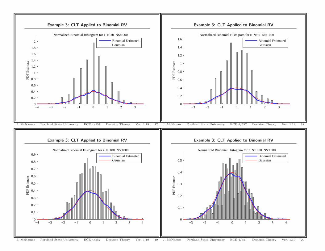
• For most data sets, n = 30 is generally accepted as large enoughfor the CLT to apply
• This is remarkable considering the theorem only applies as n → ∞• The center of the distribution becomes normally distributed more
quickly (i.e., with smaller n) than the tails
J. McNames Portland State University ECE 4/557 Decision Theory Ver. 1.19 12
Biased Estimation
• An estimator θ is an unbiased estimator of the populationparameter θ if E[θ] = θ
• Sample mean of a random sample is an unbiased estimate ofpopulation (true) mean
• Sample variance s2X = 1
n−1
∑ni=1(Xi − X)2 is unbiased estimate
of true (population) variance
– Why 1n−1?
– We lose one degree of freedom by estimating E[X] with X
– Is one of your homework problems
• sX is a biased estimate of the true population standard deviation
J. McNames Portland State University ECE 4/557 Decision Theory Ver. 1.19 10
Example 3: CLT Applied to Binomial RV
−2.5 −2 −1.5 −1 −0.5 0 0.5 1 1.5 2 2.50
0.5
1
1.5
2
2.5
3
3.5
Est
imat
e
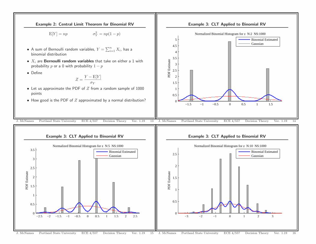
Normalized Binomial Histogram for z N:5 NS:1000
Binomial EstimatedGaussian
J. McNames Portland State University ECE 4/557 Decision Theory Ver. 1.19 15
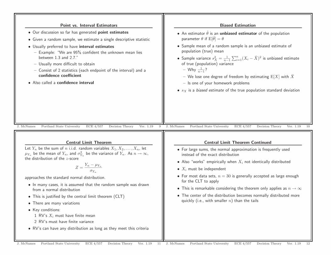
Example 2: Central Limit Theorem for Binomial RV
E[Y ] = np σ2Y = np(1 − p)
• A sum of Bernoulli random variables, Y =∑n
i=1 Xi, has abinomial distribution
• Xi are Bernoulli random variables that take on either a 1 withprobability p or a 0 with probability 1 − p
• Define
Z =Y − E[Y ]
σY
• Let us approximate the PDF of Z from a random sample of 1000points
• How good is the PDF of Z approximated by a normal distribution?
J. McNames Portland State University ECE 4/557 Decision Theory Ver. 1.19 13
Example 3: CLT Applied to Binomial RV
−3 −2 −1 0 1 2 30
0.5
1
1.5
2
2.5
Est
imat
e
Normalized Binomial Histogram for z N:10 NS:1000
Binomial EstimatedGaussian
J. McNames Portland State University ECE 4/557 Decision Theory Ver. 1.19 16
Example 3: CLT Applied to Binomial RV
−1.5 −1 −0.5 0 0.5 1 1.50
0.5
1
1.5
2
2.5
3
3.5
4
4.5
5
Est
imat
e
Normalized Binomial Histogram for z N:2 NS:1000
Binomial EstimatedGaussian
J. McNames Portland State University ECE 4/557 Decision Theory Ver. 1.19 14
Example 3: CLT Applied to Binomial RV
−4 −3 −2 −1 0 1 2 3 40
0.1
0.2
0.3
0.4
0.5
0.6
0.7
0.8
0.9
Est
imat
e
Normalized Binomial Histogram for z N:100 NS:1000
Binomial EstimatedGaussian
J. McNames Portland State University ECE 4/557 Decision Theory Ver. 1.19 19
Example 3: CLT Applied to Binomial RV
−4 −3 −2 −1 0 1 2 30
0.2
0.4
0.6
0.8
1
1.2
1.4
1.6
1.8
2
Est
imat
e
Normalized Binomial Histogram for z N:20 NS:1000
Binomial EstimatedGaussian
J. McNames Portland State University ECE 4/557 Decision Theory Ver. 1.19 17
Example 3: CLT Applied to Binomial RV
−3 −2 −1 0 1 2 3 40
0.1
0.2
0.3
0.4
0.5
Est
imat
e
Normalized Binomial Histogram for z N:1000 NS:1000
Binomial EstimatedGaussian
J. McNames Portland State University ECE 4/557 Decision Theory Ver. 1.19 20
Example 3: CLT Applied to Binomial RV
−3 −2 −1 0 1 2 30
0.2
0.4
0.6
0.8
1
1.2
1.4
1.6
Est
imat
e
Normalized Binomial Histogram for z N:30 NS:1000
Binomial EstimatedGaussian
J. McNames Portland State University ECE 4/557 Decision Theory Ver. 1.19 18

legend([h(2) h(1)],’Binomial Estimated’,’Gaussian’);
st = sprintf(’print -depsc CLTBinomial%04d’,np);
eval(st);
drawnow;
%fprintf(’Pausing...\n’); pause;
end;
J. McNames Portland State University ECE 4/557 Decision Theory Ver. 1.19 23
Example 3: CLT Applied to Binomial RV
−3 −2 −1 0 1 2 30
0.1
0.2
0.3
0.4
0.5
Est
imat
e
Normalized Binomial Histogram for z N:5000 NS:1000
Binomial EstimatedGaussian
J. McNames Portland State University ECE 4/557 Decision Theory Ver. 1.19 21
Example 4: CLT Applied to Exponential RV
−5 −4 −3 −2 −1 0 1 2 3 4 50
0.1
0.2
0.3
0.4
0.5
0.6
0.7
0.8
0.9
1
Est
imat
e
Normalized Exponential Sum Histogram for z N:1 NS:1000
Exponential Sum EstimatedGaussian
J. McNames Portland State University ECE 4/557 Decision Theory Ver. 1.19 24
Example 3: MATLAB Codefunction [] = CLTBinomial();
close all;
FigureSet(1,’LTX’);NP = [2,5,10,20,30,100,1000,5000]; % No. histogramsNS = 1000; % No. Samplesp = 0.5; % Probability of 1
for cnt = 1:length(NP),np = NP(cnt);r = binornd(np,p,NS,1); % Random sample of NS sumsmu = np*p;s2 = np*p*(1-p);z = (r-mu)/sqrt(s2);figure;FigureSet(1,’LTX’);Histogram(z,0.1,0.20);hold on;
x = -5:0.02:5;y1 = 1/sqrt(2*pi).*exp(-x.^2/2);h = plot(x,y1,’r’);x2 = 0:np;y2 = binopdf(x2,np,p);x2 = (x2-mu)/sqrt(s2);%h = goodstem(x2,y2,’g’);%set(h,’LineWidth’,1.5);hold off;
%set(gca,’XLim’,[-5 5]);st = sprintf(’Normalized Binomial Histogram for z N:%d NS:%d’,np,NS);title(st);box off;AxisSet(8);h = get(gca,’Children’);
J. McNames Portland State University ECE 4/557 Decision Theory Ver. 1.19 22
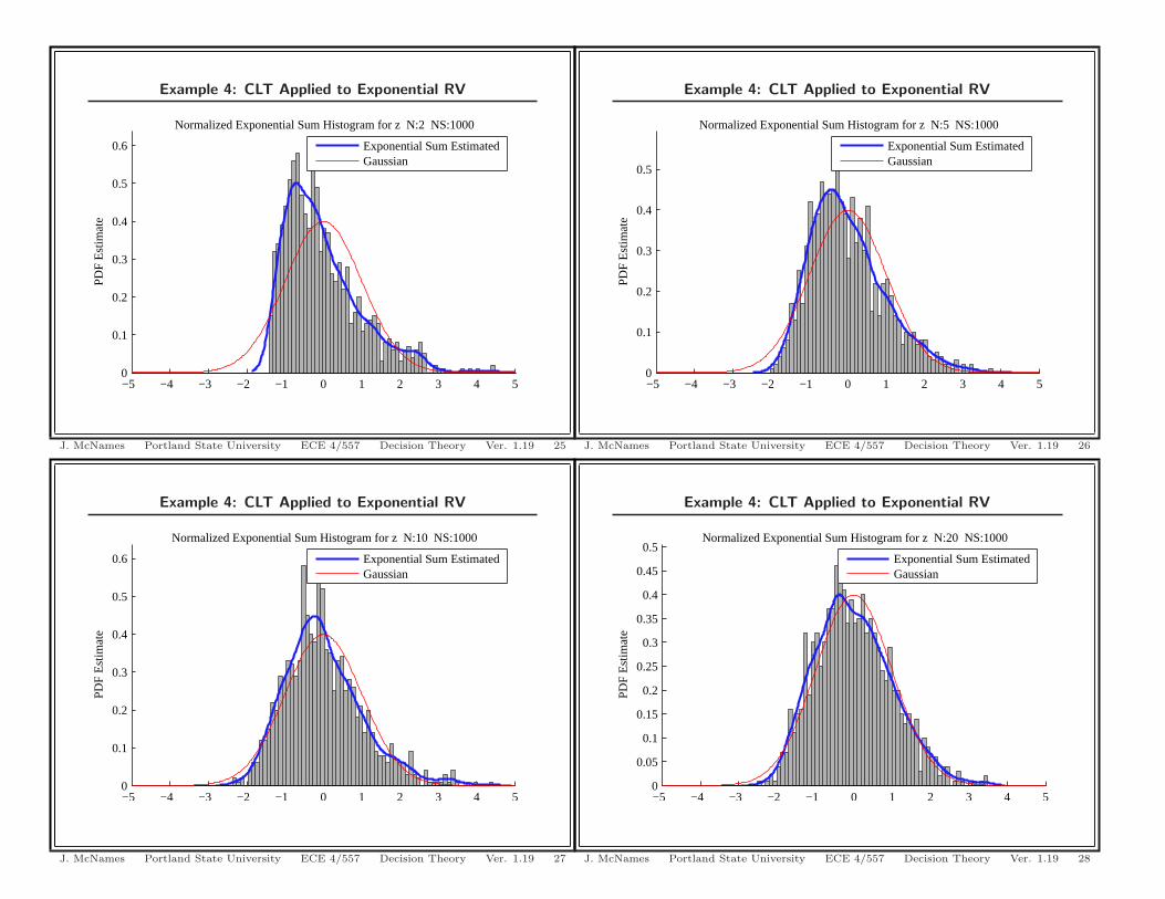
Example 4: CLT Applied to Exponential RV
−5 −4 −3 −2 −1 0 1 2 3 4 50
0.1
0.2
0.3
0.4
0.5
0.6
Est
imat
e
Normalized Exponential Sum Histogram for z N:10 NS:1000
Exponential Sum EstimatedGaussian
J. McNames Portland State University ECE 4/557 Decision Theory Ver. 1.19 27
Example 4: CLT Applied to Exponential RV
−5 −4 −3 −2 −1 0 1 2 3 4 50
0.1
0.2
0.3
0.4
0.5
0.6
Est
imat
e
Normalized Exponential Sum Histogram for z N:2 NS:1000
Exponential Sum EstimatedGaussian
J. McNames Portland State University ECE 4/557 Decision Theory Ver. 1.19 25
Example 4: CLT Applied to Exponential RV
−5 −4 −3 −2 −1 0 1 2 3 4 50
0.05
0.1
0.15
0.2
0.25
0.3
0.35
0.4
0.45
0.5
Est
imat
e
Normalized Exponential Sum Histogram for z N:20 NS:1000
Exponential Sum EstimatedGaussian
J. McNames Portland State University ECE 4/557 Decision Theory Ver. 1.19 28
Example 4: CLT Applied to Exponential RV
−5 −4 −3 −2 −1 0 1 2 3 4 50
0.1
0.2
0.3
0.4
0.5
Est
imat
e
Normalized Exponential Sum Histogram for z N:5 NS:1000
Exponential Sum EstimatedGaussian
J. McNames Portland State University ECE 4/557 Decision Theory Ver. 1.19 26
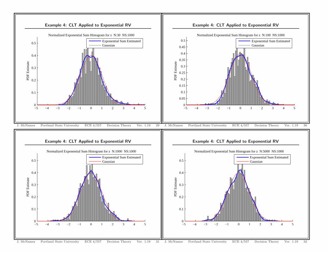
Example 4: CLT Applied to Exponential RV
−5 −4 −3 −2 −1 0 1 2 3 4 50
0.1
0.2
0.3
0.4
0.5
Est
imat
e
Normalized Exponential Sum Histogram for z N:1000 NS:1000
Exponential Sum EstimatedGaussian
J. McNames Portland State University ECE 4/557 Decision Theory Ver. 1.19 31
Example 4: CLT Applied to Exponential RV
−5 −4 −3 −2 −1 0 1 2 3 4 50
0.1
0.2
0.3
0.4
0.5
Est
imat
e
Normalized Exponential Sum Histogram for z N:30 NS:1000
Exponential Sum EstimatedGaussian
J. McNames Portland State University ECE 4/557 Decision Theory Ver. 1.19 29
Example 4: CLT Applied to Exponential RV
−5 −4 −3 −2 −1 0 1 2 3 4 50
0.1
0.2
0.3
0.4
0.5
Est
imat
e
Normalized Exponential Sum Histogram for z N:5000 NS:1000
Exponential Sum EstimatedGaussian
J. McNames Portland State University ECE 4/557 Decision Theory Ver. 1.19 32
Example 4: CLT Applied to Exponential RV
−5 −4 −3 −2 −1 0 1 2 3 4 50
0.05
0.1
0.15
0.2
0.25
0.3
0.35
0.4
0.45
0.5
Est
imat
e
Normalized Exponential Sum Histogram for z N:100 NS:1000
Exponential Sum EstimatedGaussian
J. McNames Portland State University ECE 4/557 Decision Theory Ver. 1.19 30

Approximate Confidence Intervals
Let Yn be the sum of n i.i.d. random variables X1, X2, . . . , Xn,
Yn =n∑
i=1
Xi
and let μX be the mean of Xi and σ2X be the variance of Xi. As
n → ∞, the distribution of
Z =Yn − nμX√
nσ2X
=X − μX
σX/√
n
approaches the standard normal distribution.
J. McNames Portland State University ECE 4/557 Decision Theory Ver. 1.19 35
Example 4: MATLAB Codefunction [] = CLTExponential();
close all;
FigureSet(1,’LTX’);NP = [1,2,5,10,20,30,100,1000,5000]; % No. histogramsNS = 1000; % No. Samplesp = 0.5; % Probability of 1lambda = 2; % Exponential Parameter
for cnt = 1:length(NP),np = NP(cnt);r = exprnd(1/lambda,np,NS); % Random sample of NS sumsif np~=1,
r = sum(r);end;
mu = np/lambda;s2 = np/lambda^2;z = (r-mu)/sqrt(s2);figure;FigureSet(1,’LTX’);Histogram(z,0.1,0.20);hold on;
x = -5:0.02:5;y1 = 1/sqrt(2*pi).*exp(-x.^2/2);h = plot(x,y1,’r’);x2 = 0:np;y2 = binopdf(x2,np,p);x2 = (x2-mu)/sqrt(s2);hold off;
set(gca,’XLim’,[-5 5]);st = sprintf(’Normalized Exponential Sum Histogram for z N:%d NS:%d’,np,NS);title(st);AxisSet(8);
J. McNames Portland State University ECE 4/557 Decision Theory Ver. 1.19 33
Approximate Confidence Intervals Continued 1
Thus, we may approximate the probability that Z is within aninterquantile range
Pr{−z1−α/2 ≤ X − μX
σX/√
n≤ z1−α/2
}= 1 − α
Note −z1-α/2 = zα/2 because the normal distribution is symmetricabout the mean.
This can be rearranged as
Pr{
X − z1−α/2σX√
n≤ μX ≤ X + z1−α/2
σX√n
}= 1 − α
• σX is seldom known
• Usually approximate with usual sample estimate
σX =√
s2X
J. McNames Portland State University ECE 4/557 Decision Theory Ver. 1.19 36
box off;
h = get(gca,’Children’);
legend([h(2) h(1)],’Exponential Sum Estimated’,’Gaussian’);
st = sprintf(’print -depsc CLTExponential%04d’,np);
eval(st);
drawnow;
end;
J. McNames Portland State University ECE 4/557 Decision Theory Ver. 1.19 34
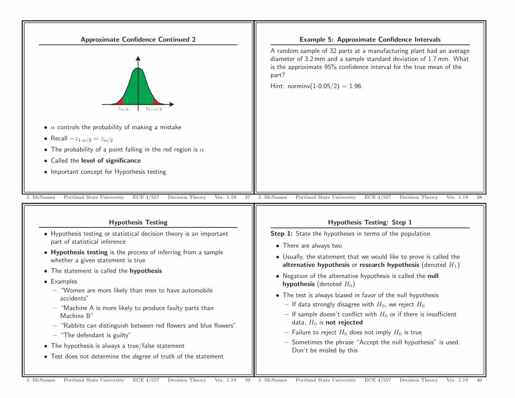
Hypothesis Testing
• Hypothesis testing or statistical decision theory is an importantpart of statistical inference
• Hypothesis testing is the process of inferring from a samplewhether a given statement is true
• The statement is called the hypothesis
• Examples
– “Women are more likely than men to have automobileaccidents”
– “Machine A is more likely to produce faulty parts thanMachine B”
– “Rabbits can distinguish between red flowers and blue flowers”
– “The defendant is guilty”
• The hypothesis is always a true/false statement
• Test does not determine the degree of truth of the statement
J. McNames Portland State University ECE 4/557 Decision Theory Ver. 1.19 39
Approximate Confidence Continued 2
zα/2 z1−α/2
• α controls the probability of making a mistake
• Recall −z1-α/2 = zα/2
• The probability of a point falling in the red region is α
• Called the level of significance
• Important concept for Hypothesis testing
J. McNames Portland State University ECE 4/557 Decision Theory Ver. 1.19 37
Hypothesis Testing: Step 1
Step 1: State the hypotheses in terms of the population.
• There are always two
• Usually, the statement that we would like to prove is called thealternative hypothesis or research hypothesis (denoted H1)
• Negation of the alternative hypothesis is called the nullhypothesis (denoted H0)
• The test is always biased in favor of the null hypothesis
– If data strongly disagree with H0, we reject H0
– If sample doesn’t conflict with H0 or if there is insufficientdata, H0 is not rejected
– Failure to reject H0 does not imply H0 is true
– Sometimes the phrase “Accept the null hypothesis” is used.Don’t be misled by this
J. McNames Portland State University ECE 4/557 Decision Theory Ver. 1.19 40
Example 5: Approximate Confidence Intervals
A random sample of 32 parts at a manufacturing plant had an averagediameter of 3.2 mm and a sample standard deviation of 1.7 mm. Whatis the approximate 95% confidence interval for the true mean of thepart?
Hint: norminv(1-0.05/2) = 1.96.
J. McNames Portland State University ECE 4/557 Decision Theory Ver. 1.19 38

Hypothesis Testing Example Continued
Step 3: Pick the decision rule.The necessary quantiles of a normal distribution are given by
z0.05/2 = −1.9600 z1−0.05/2 = 1.9600z0.01/2 = −2.5758 z1−0.01/2 = 2.5758
Step 4: Evaluate T and make decision.
T =X − μ
σ/√
n=
523 − 50097/
√100
= 2.3711
We reject H0 at the 0.05 significance level.We fail to reject H0 at the 0.01 significance level.
J. McNames Portland State University ECE 4/557 Decision Theory Ver. 1.19 43
Hypothesis Testing: Steps 2–4
Step 2: Select a test statistic T .
• Want test statistic to take on some values when H0 is true
• Want to taken on others when H1 is true
• Want to be sensitive indicator of whether the data agree ordisagree with H0
• Test statistic is usually chosen such that its distribution is known(at least approximately) when H0 is true
Step 3: Pick the decision rule.
• Choose a decision rule in terms of the possible values of T
• Usually accompanied by the level of significance α
Step 4: Based on the random sample, evaluate T and make a decision
J. McNames Portland State University ECE 4/557 Decision Theory Ver. 1.19 41
Hypothesis Testing: Definitions
Upper Tailed Test Two Tailed TestLower Tailed Test
zαz1−α zα/2 z1−α/2
• Critical Region: the set of all points in the sample space thatresult in the decision to reject H0
• Acceptance Region: the set of all points in the sample space notin the critical region
• Upper-Tailed Test: H0 is rejected for large values of T
• Lower-Tailed Test: H0 is rejected for small values of T
• Two-Tailed Test: H0 is rejected for large or small values of T
J. McNames Portland State University ECE 4/557 Decision Theory Ver. 1.19 44
Hypothesis Testing Example
The average lifetime of a sample of 100 integrated circuits (IC) is 523days with a standard deviation of 97 days. If μ is the mean lifetime ofall the IC’s produced by the company, test the hypothesis μ = 500days against the alternative hypothesis μ �= 500 days using levels ofsignificance 0.05 and 0.01.
Step 1: The hypotheses are stated in terms of the population.H0: μ = 500 daysH1: μ �= 500 days
Step 2: Select a test statistic T .Since n = 100, we can assume the CLT applies and let us use as ourtest statistic
T =X − μ
s/√
n
By the CLT, we know the distribution is approximately normal.
J. McNames Portland State University ECE 4/557 Decision Theory Ver. 1.19 42
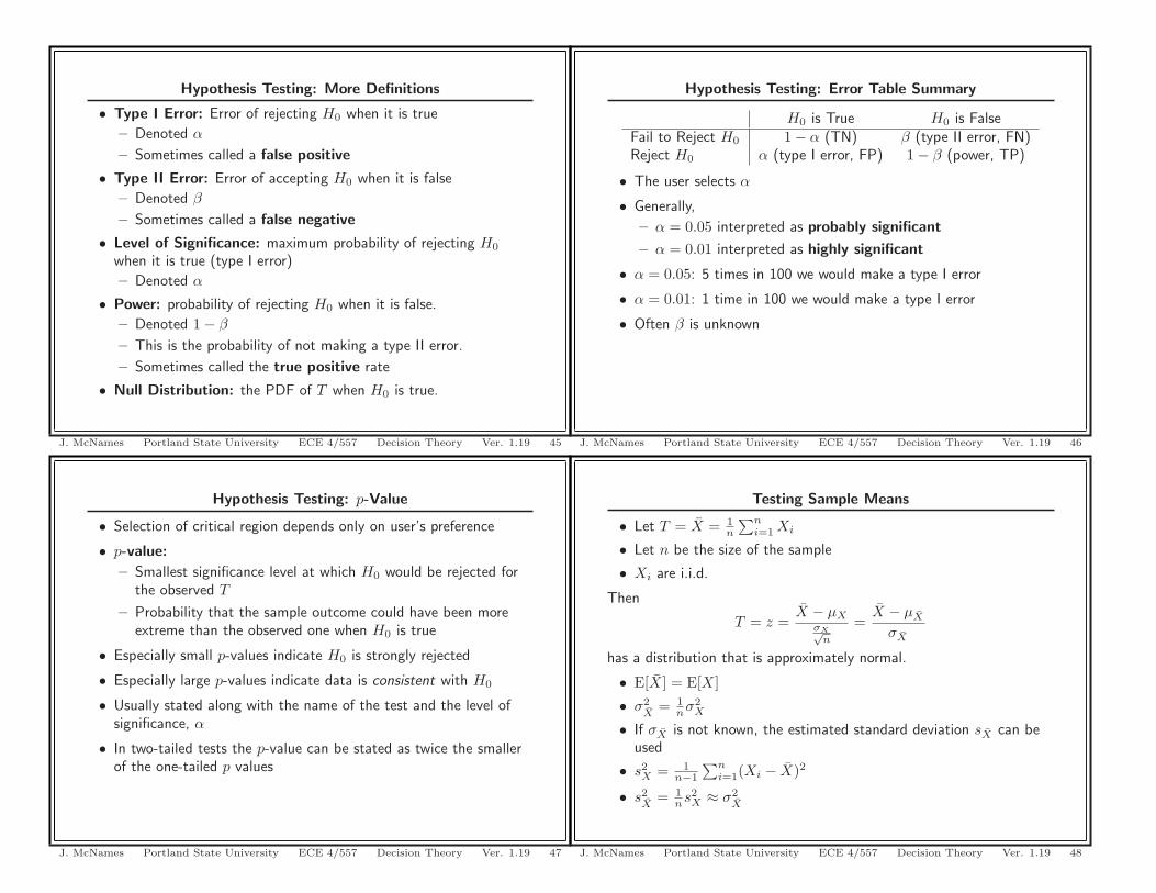
Hypothesis Testing: p-Value
• Selection of critical region depends only on user’s preference
• p-value:
– Smallest significance level at which H0 would be rejected forthe observed T
– Probability that the sample outcome could have been moreextreme than the observed one when H0 is true
• Especially small p-values indicate H0 is strongly rejected
• Especially large p-values indicate data is consistent with H0
• Usually stated along with the name of the test and the level ofsignificance, α
• In two-tailed tests the p-value can be stated as twice the smallerof the one-tailed p values
J. McNames Portland State University ECE 4/557 Decision Theory Ver. 1.19 47
Hypothesis Testing: More Definitions
• Type I Error: Error of rejecting H0 when it is true
– Denoted α
– Sometimes called a false positive
• Type II Error: Error of accepting H0 when it is false
– Denoted β
– Sometimes called a false negative
• Level of Significance: maximum probability of rejecting H0
when it is true (type I error)
– Denoted α
• Power: probability of rejecting H0 when it is false.
– Denoted 1 − β
– This is the probability of not making a type II error.
– Sometimes called the true positive rate
• Null Distribution: the PDF of T when H0 is true.
J. McNames Portland State University ECE 4/557 Decision Theory Ver. 1.19 45
Testing Sample Means
• Let T = X = 1n
∑ni=1 Xi
• Let n be the size of the sample
• Xi are i.i.d.
Then
T = z =X − μX
σX√n
=X − μX
σX
has a distribution that is approximately normal.
• E[X] = E[X]
• σ2X
= 1nσ2
X
• If σX is not known, the estimated standard deviation sX can beused
• s2X = 1
n−1
∑ni=1(Xi − X)2
• s2X
= 1ns2
X ≈ σ2X
J. McNames Portland State University ECE 4/557 Decision Theory Ver. 1.19 48
Hypothesis Testing: Error Table Summary
H0 is True H0 is FalseFail to Reject H0 1 − α (TN) β (type II error, FN)Reject H0 α (type I error, FP) 1 − β (power, TP)
• The user selects α
• Generally,
– α = 0.05 interpreted as probably significant
– α = 0.01 interpreted as highly significant
• α = 0.05: 5 times in 100 we would make a type I error
• α = 0.01: 1 time in 100 we would make a type I error
• Often β is unknown
J. McNames Portland State University ECE 4/557 Decision Theory Ver. 1.19 46

Testing Proportions
• Consider a binary criterion or test that yields either a success orfailure.
• Let T = p where p is the proportion of successes
• Let n be the size of the sample
• Let p denote the proportion of “true” successes (if the test wereapplied to the entire population)
Then
z =p − p√p(1−p)
n
has a distribution that is approximately normal.
• σ2 = p(1−p)n
J. McNames Portland State University ECE 4/557 Decision Theory Ver. 1.19 51
Example 6: Sample Means
An IC manufacturer knows that their integrated circuits have a meanmaximum operating frequency of 500 MHz with a standard deviationof 50 MHz. With a new process, it is claimed that the maximumoperating frequency can be increased. To test this claim, a sample of50 IC’s were tested and it was found that the average maximumoperating frequency was 520 MHz. Can we support the claim at the0.01 significance level? Hint: z1−0.01 = 2.3263 and z0.9977 = 2.8284.
J. McNames Portland State University ECE 4/557 Decision Theory Ver. 1.19 49
Example 7: Testing Proportions
A student in ECE 4/557 class creates an algorithm to predict whetherIntel’s stock will increase or decrease. The algorithm is tested on theclosing price over a period of 31 days (1 month). The algorithmcorrectly predicted increases and decreases in 20 of the 31 days.Determine whether the results are significant (better than chance) atthe 0.05 and 0.01 significance levels. Hints: z1−0.05/2 = 1.96,z1−0.01/2 = 2.5758, z1−0.05 = 1.6449, z1−0.01 = 2.3263,z0.9470 = 1.6164.
J. McNames Portland State University ECE 4/557 Decision Theory Ver. 1.19 52
Example 6: Workspace
J. McNames Portland State University ECE 4/557 Decision Theory Ver. 1.19 50
Small Sample Mean Tests
Suppose we have a random sample of n observations X1, X2, . . . Xn
that is drawn independently from a normal population with mean μand standard deviation σ. As before, the sample mean and standarddeviation are given by
X =1n
n∑i=1
Xi sX =
√√√√ 1n − 1
n∑i=1
(Xi − X)2
and the estimated standard deviation of X is given by sX = sX√n
Then
the normalized random variable
T =X − μ
sX
is distributed as the student’s t distribution with n − 1 degrees offreedom.
J. McNames Portland State University ECE 4/557 Decision Theory Ver. 1.19 55
Example 7: Workspace
J. McNames Portland State University ECE 4/557 Decision Theory Ver. 1.19 53
Small Sample Mean Tests Comments
• The approach is the same as before
• Only difference: different distribution
• t distribution is symmetric
• MATLAB functions: tinv, tcdf, & tpdf
• Confidence intervals for μ: X ± t(1 − α/2; n − 1)sX
• For large n, the t distribution is approximately normal
J. McNames Portland State University ECE 4/557 Decision Theory Ver. 1.19 56
Small Sampling Theory
• Test statistics are often chosen as sums of values in a sample sothat CLT applies and the normal distribution can be assumed
• Only considered valid for large samples (say n > 30)
• For small samples, many other tricks can be used
• If the values being recorded are known to come from a Gaussiandistribution, the t tests can be used
J. McNames Portland State University ECE 4/557 Decision Theory Ver. 1.19 54

Example 9: Small Sample Mean Tests
Choose between the alternatives
H0 :μ ≤ 20H1 :μ > 20
when α is to be controlled at 0.05, n = 13, X = 24 and sX = 5.Hints: tinv(0.95,12) = 1.7823 and 1-tcdf(2.88,12) = 0.0069.
J. McNames Portland State University ECE 4/557 Decision Theory Ver. 1.19 59
Small Sample Mean Tests Concise Summary
T =X − μ
sX
H0: μ = μ0 If |T | ≤ t(1 − α/2; n − 1), conclude H0
H1: μ �= μ0 If |T | > t(1 − α/2; n − 1), conclude H1
H0: μ ≥ μ0 If T ≥ t(α; n − 1), conclude H0
H1: μ < μ0 If T < t(α; n − 1), conclude H1
H0: μ ≤ μ0 If T ≤ t(1 − α; n − 1), conclude H0
H1: μ > μ0 If T > t(1 − α; n − 1), conclude H1
J. McNames Portland State University ECE 4/557 Decision Theory Ver. 1.19 57
Example 10: Small Sample Mean Tests
Choose between the alternatives
H0 :μ = 10H1 :μ �= 10
when α is to be controlled at 0.02, n = 15, X = 14 and sX = 6.Hints: tinv(1-0.02/2,14) = 2.6245 and 2*(1-tcdf(2.582,14)) = 0.0217.
J. McNames Portland State University ECE 4/557 Decision Theory Ver. 1.19 60
Example 8: Small Sample Mean Tests
Students in ECE 4/557 chose 10 pairs of numbers “close to 5.” Themean of the first set of numbers was 4.8837 with a sample standarddeviation of 0.3165. The second set had X = 5.1198 andsX = 0.3157. Assuming each set was drawn from a normaldistribution, determine whether each set was drawn from a distributionwith a mean of 5.
Hints: tinv(1-0.05/2,9) = 2.2622,1-tcdf(abs((4.8837-5)/(0.3165/sqrt(10))),9)=0.1376,1-tcdf(abs((5.1198-5)/(0.3157/sqrt(10))),9)=0.1304.
J. McNames Portland State University ECE 4/557 Decision Theory Ver. 1.19 58
Example 11: Two Population Means
Students in ECE 4/557 chose 10 pairs of numbers “close to 5.” Themean of the first set of numbers was X = 4.8837 with a samplestandard deviation of sX = 0.3165. The second set had Y = 5.1198and sY = 0.3157. Assuming each set was drawn from a normaldistribution, determine whether each was drawn from a distributionwith the same mean.
Hint: s = 0.0999, tinv(1-0.05/2,18) = 2.101.
J. McNames Portland State University ECE 4/557 Decision Theory Ver. 1.19 63
Comparing Two Population Means
Let there be two normal populations with two means μX and μY andthe same standard deviation σ. The means μx and μy are to becompared for the two populations. Define estimators of the twosample means and the common standard deviation as follows
X =1nx
nx∑i=1
Xi Y =1ny
ny∑i=1
Yi
s2 =∑nx
i=1(Xi − X)2 +∑ny
i=1(Yi − Y )2
nx + ny − 2
The variance of the difference σ2X−Y
can be estimated as
s2X−Y = s2
(1nx
+1ny
)
J. McNames Portland State University ECE 4/557 Decision Theory Ver. 1.19 61
Example 12: Two Population Means
Obtain a 95% confidence interval for μX − μY when
nX = 10 X = 14∑
(Xi − X)2 = 105
nY = 20 Y = 8∑
(Yi − Y )2 = 224
Hints: tinv(0.05/2,28) = -2.0484.
J. McNames Portland State University ECE 4/557 Decision Theory Ver. 1.19 64
Comparing Two Population Means Summary
T =X − Y
sX−Y
has a t distribution with nx + ny − 2 degrees of freedom
Confidence Limits:
(X − Y ) ± t(1 − α/2; nx + nY − 2)sX−Y
Hypothesis Tests:H0: μX = μY If |T | ≤ t(1 − α/2; nX + nY − 2), conclude H0
H1: μX �= μY If |T | > t(1 − α/2; nX + nY − 2), conclude H1
H0: μX ≥ μY If T ≥ t(α; nX + nY − 2), conclude H0
H1: μX < μY If T < t(α; nX + nY − 2), conclude H1
H0: μX ≤ μY If T ≤ t(1 − α; nX + nY − 2), conclude H0
H1: μX > μY If T > t(1 − α; nX + nY − 2), conclude H1
J. McNames Portland State University ECE 4/557 Decision Theory Ver. 1.19 62

Population Variance Inference Summary
T =(n − 1)s2
σ20
Confidence Limits:
(n − 1)s2
χ2(1 − α/2; n − 1)≤ σ2 ≤ (n − 1)s2
χ2(α/2; n − 1)
Hypothesis Tests:H0: σ2 = σ2
0 If χ2(α/2; n − 1) ≤ T ≤ χ2(1 − α/2; n − 1),H1: σ2 �= σ2
0 conclude H0. Otherwise, conclude H1
H0: σ2 ≥ σ20 If T ≥ χ2(α; n − 1), conclude H0
H1: σ2 < σ20 If T < χ2(α; n − 1), conclude H1
H0: σ2 ≤ σ20 If T ≤ χ2(1 − α; n − 1), conclude H0
H1: σ2 > σ20 If T > χ2(1 − α; n − 1), conclude H1
J. McNames Portland State University ECE 4/557 Decision Theory Ver. 1.19 67
Example 13: Two Population Means
Choose between the alternatives
H0 :μ1 = μ2
H1 :μ1 �= μ2
with 0.10 level of confidence. Same data as the previous example.
Hints: tinv(0.95,28) = 1.07011 and 1-tcdf(4.52,28) = 0.000051.
J. McNames Portland State University ECE 4/557 Decision Theory Ver. 1.19 65
Example 14: Population Variance Inference
Obtain a 98% confidence interval for σ2. The data consists of 10points with s = 4.
Hints: chi2inv(0.01,9) = 2.088 and chi2inv(0.99,9) = 21.666.
J. McNames Portland State University ECE 4/557 Decision Theory Ver. 1.19 68
Population Variance Inference
When sampling from a normal population and the sample variance isgiven by s2,
(n − 1)s2
σ2
is distributed as χ2 with n − 1 degrees of freedom.
• The χ2 is just another distribution
• It is also the distribution of∑n
i=1 X2i where Xi ∼ N (0, 1) (i.e.
Xis are RV’s drawn from a standard normal distribution) and n isthe degrees of freedom
• χ2 is not symmetric
• The rules and concepts are the same
J. McNames Portland State University ECE 4/557 Decision Theory Ver. 1.19 66

Example 15: Two Population Variances
Obtain a 90% confidence interval for σ2X/σ2
Y when the data are
nX = 16 nY = 21
s2X = 54.2 s2
Y = 17.8
Hints: finv(0.05,15,20) = 0.4296, finv(0.95,15,20) = 2.2033.
J. McNames Portland State University ECE 4/557 Decision Theory Ver. 1.19 71
Comparing Two Population Variances
Let independent samples be drawn from two normal populations withmeans and variances μX and σ2
X and μY and σ2Y , respectively. The
sample variances are
s2X =
1nX − 1
nX∑i=1
(Xi − X)2 s2Y =
1nY − 1
nY∑i=1
(Yi − Y )2
Thens2
X
σ2X
s2Y
σ2Y
is distributed as F (nx − 1, nY − 1).
The F test is sensitive to departures from the normality assumption.
J. McNames Portland State University ECE 4/557 Decision Theory Ver. 1.19 69
Example 16: Two Population Variances
Choose between the alternatives
H0 :σ2X = σ2
Y
H1 :σ2X �= σ2
X
with α controlled at 0.02.
nX = 16 nY = 21
s2X = 54.2 s2
Y = 17.8
Hints: finv(0.01,15,20) = 0.2966, finv(0.99,15,20) = 3.09.
J. McNames Portland State University ECE 4/557 Decision Theory Ver. 1.19 72
Comparing Two Population Variances Summary
T =s2
X
s2Y
Confidence Limits:
s2X
s2Y
1F (1 − α/2; nX − 1, nY − 1)
≤ σ2X
σ2Y
≤ s2X
s2Y
1F (α/2; nX − 1, nY − 1)
Hypothesis Tests:H0: σ2
X = σ2Y If F (α/2; nX -1, nY -1) ≤ T ≤ F (1 − α/2; nX -1, nY -1),
H1: σ2X �= σ2
Y conclude H0. Otherwise, conclude H1
H0: σ2X ≥ σ2
Y If T ≥ F (α; nX − 1, nY − 1), conclude H0
H1: σ2X < σ2
Y If T < F (α; nX − 1, nY − 1), conclude H1
H0: σ2X ≤ σ2
Y If T ≤ F (1 − α; nX − 1, nY − 1), conclude H0
H1: σ2X > σ2
Y If T > F (1 − α; nX − 1, nY − 1), conclude H1
J. McNames Portland State University ECE 4/557 Decision Theory Ver. 1.19 70
Parametric vs. Nonparametric
• Parametric methods
– depend on knowledge of F (x)– The parameter values may be unknown
– How can we be certain F (x) is really what we think it is?
– If we are certain, the parametric test is probably the mostpowerful
– All tests discussed so far are parametric
– Good for light tails, poor for heavy tails (outliers)
• Nonparametric = distribution free
– No assumption about F (x)– Apply to all distributions
– Always work well
– Usually best with heavy tails (outliers)
J. McNames Portland State University ECE 4/557 Decision Theory Ver. 1.19 75
Parametric versus Nonparametric Introduction
• After a model for an experiment has been defined, to conduct atest, the probabilities associated with the model must be found
• This can be very hard
• Statisticians have often changed the model slightly to solve for theprobabilities
• Change is slight enough to ensure model is realistic
• Can then find exact solutions to approximate problems
• This is parametric statistics
• Includes tests we have discussed
J. McNames Portland State University ECE 4/557 Decision Theory Ver. 1.19 73
Nonparametric Defined
A statistical method is nonparametric if it satisfies at least one of thefollowing criteria
1. May be used on nominal data
2. May be used on ordinal data
3. May be used on interval or ratio data where the distribution isunspecified
J. McNames Portland State University ECE 4/557 Decision Theory Ver. 1.19 76
Parametric versus Nonparametric Introduction Continued
• Caught momentum in the late 1930s
• Makes few assumptions
• Simple methods to find good approximation of probabilities
• Can the find approximate solutions to exact problems
• Safer than parametric methods
• Use when price of making wrong decision is high
• Often require less computation
• Most of the theory is fairly simple
• Often more powerful than parametric methods
J. McNames Portland State University ECE 4/557 Decision Theory Ver. 1.19 74
Example 17: Binomial Test
A company estimates that 20% of the die they manufacture are faulty.A new method is developed to reduce the number of faulty die. Out of29 die, only 3 were faulty. Is it safe to conclude that the new methodreduces the number of faulty die at a 0.05 level of significance? Whatis the p value?
Hint: binocdf(3,29,0.20) = 0.1404.
J. McNames Portland State University ECE 4/557 Decision Theory Ver. 1.19 79
More Definitions
Unbiased Test: test in which the probability of rejecting H0 whenH0 is false is always greater than or equal to the probability ofrejecting H0 when H0 is true
Consistent Test: test in which the power approaches 1 as thesample size approaches infinity for some fixed level of significanceα > 0
Conservative Test: test in which the actual level of significance issmaller than the stated level
Robust Test: test that is approximately valid even if theassumptions behind the method are not true
• The t test is robust against normality
J. McNames Portland State University ECE 4/557 Decision Theory Ver. 1.19 77
Example 18: Binomial Test
A circuit is expected to produce a true output (1) 80% of the time.The technician suspects the circuit is not working. Out of 682 clockcycles, the circuit produced 520 true outputs. With a 0.01 level ofsignificance, can we say the circuit is not working? What is the pvalue?
Hints: binocdf(520,682,0.8) = 0.0091.
J. McNames Portland State University ECE 4/557 Decision Theory Ver. 1.19 80
The Binomial Test
• Goal: Is p∗ the probability of Class 1?
• Data: Two classes: Class 1 or Class 2 (not both)
• Definitions
– n1 = observations in class 1
– n2 = observations in class 2
– n = number of observations
• Assumptions
– The n trials are independent
– Each trial has a probability p of generating class 1
• Test statistic: n1
• Null Distribution: Binomial with probability p
J. McNames Portland State University ECE 4/557 Decision Theory Ver. 1.19 78

Binomial Confidence Intervals on p
• Same data and assumptions as before
• p is unknown
• What is the x% confidence interval on p?
• Can be obtained directly from MATLAB’s binofit function
J. McNames Portland State University ECE 4/557 Decision Theory Ver. 1.19 83
Example 19: Binomial Test
A researcher finds what they believe is a significant leading indicator ofthe outcome of Trail Blazers’ games. The indicator was used toprospectively generate a correct outcome in 11 out of 15 games.Determine whether the results are significant (better than chance) atthe 0.05 significance level. Hints: 1-binocdf(10,15,0.5) = 0.0592,1-binocdf(11,15,0.5) = 0.0176.
J. McNames Portland State University ECE 4/557 Decision Theory Ver. 1.19 81
Example 21: Binomial Confidence Intervals
Twenty students were selected at random to see if they could do nodalanalysis in ECE 221. Seven students could successfully complete theproblems. What is a 95% confidence interval of p, the proportion ofstudents in the class who could do nodal analysis?
Answer: [phat,pci] = binofit(7,20)
p = 0.35 and with 95% confidence 0.1539 ≤ p ≤ 0.5922
J. McNames Portland State University ECE 4/557 Decision Theory Ver. 1.19 84
Example 20: Binomial Test
A student in ECE 4/557 class creates an algorithm to predict whetherIntel’s stock will increase or decrease. The algorithm is tested on theclosing price over a period of 31 days (1 month). The algorithmcorrectly predicted increases and decreases in 20 of the 31 days.Determine whether the results are significant (better than chance) atthe 0.05 significance level. Hints: 1-binocdf(19,31,0.5) = 0.0592,1-binocdf(20,31,0.5) = 0.0354.
J. McNames Portland State University ECE 4/557 Decision Theory Ver. 1.19 82
The Sign Test
• Goal: Does one variable in a pair (X, Y ) tend to be larger thanthe other?
• Data:
– If X > Y classified as +– If X < Y , classified as −– If X = Y , classified as 0
• Definitions:
– n = No. of untied pairs
– p = stated P (X = Y )
• Assumptions:
– The data is i.i.d.
– The measurement scale is at least ordinal
• Test statistic: T = No. of +’s
• Null Distribution: Binomial with probability 12
J. McNames Portland State University ECE 4/557 Decision Theory Ver. 1.19 87
The Quantile Test
• Goal: Is x∗ the p∗ quantile of F (X)?
• Data: x1, x2, . . . , xn
• Definitions:
– n = No. observations
– p = stated probability p
• Assumptions:
– The data is i.i.d.
– The measurement scale is at least ordinal
• Test statistic: T = No. observations ≤ x∗
• Null Distribution: Binomial with probability p
J. McNames Portland State University ECE 4/557 Decision Theory Ver. 1.19 85
Example 23: Sign Test
A student develops a new method of analyzing DC circuits containingop amps. He wishes to determine whether the new method is fasterthan the method described in class. He selects 10 problems andmeasures the time required to solve the problem using each of themethods. He receives the following results
• 8 = No. +’s
• 1 = No. −’s
• 1 = No. ties
Is the new method faster with a 0.05 level of significance? What is thep value?
Hints: 1-binocdf(8,9,0.5)=0.002 ,1-binocdf(7,9,0.5) = 0.0195.
J. McNames Portland State University ECE 4/557 Decision Theory Ver. 1.19 88
Example 22: Quantile Test
It has been well established that the upper quartile of exam scores atPortland State is 85%. A statistics professor is concerned about gradeinflation and randomly selects an exam score from 15 classes. Sheobtains the following data
72 63 91 87 8293 78 79 82 8546 60 94 87 86
HypothesesH0: The upper quartile is 85%H1: The upper quartile is not 85%
Hints: binocdf(8,15,0.75) = 0.0566, binocdf(9,15,0.75) = 0.1484.
J. McNames Portland State University ECE 4/557 Decision Theory Ver. 1.19 86
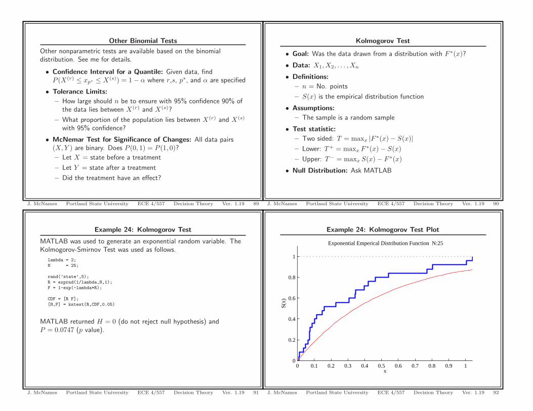
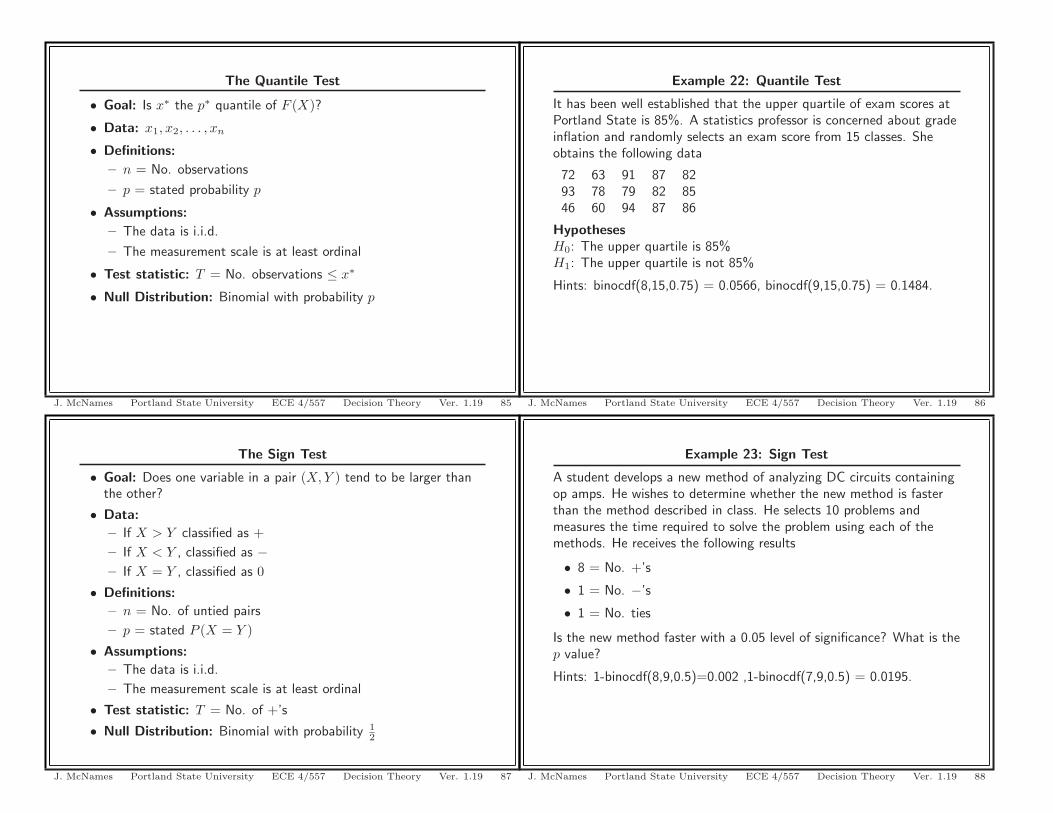
Example 24: Kolmogorov Test
MATLAB was used to generate an exponential random variable. TheKolmogorov-Smirnov Test was used as follows.
lambda = 2;N = 25;
rand(’state’,5);R = exprnd(1/lambda,N,1);F = 1-exp(-lambda*R);
CDF = [R F];[H,P] = kstest(R,CDF,0.05)
MATLAB returned H = 0 (do not reject null hypothesis) andP = 0.0747 (p value).
J. McNames Portland State University ECE 4/557 Decision Theory Ver. 1.19 91
Other Binomial Tests
Other nonparametric tests are available based on the binomialdistribution. See me for details.
• Confidence Interval for a Quantile: Given data, findP (X(r) ≤ xp∗ ≤ X(s)) = 1 − α where r,s, p∗, and α are specified
• Tolerance Limits:
– How large should n be to ensure with 95% confidence 90% ofthe data lies between X(r) and X(s)?
– What proportion of the population lies between X(r) and X(s)
with 95% confidence?
• McNemar Test for Significance of Changes: All data pairs(X, Y ) are binary. Does P (0, 1) = P (1, 0)?– Let X = state before a treatment
– Let Y = state after a treatment
– Did the treatment have an effect?
J. McNames Portland State University ECE 4/557 Decision Theory Ver. 1.19 89
Example 24: Kolmogorov Test Plot
0 0.1 0.2 0.3 0.4 0.5 0.6 0.7 0.8 0.9 10
0.2
0.4
0.6
0.8
1
x
S(x)
Exponential Emperical Distribution Function N:25
J. McNames Portland State University ECE 4/557 Decision Theory Ver. 1.19 92
Kolmogorov Test
• Goal: Was the data drawn from a distribution with F ∗(x)?
• Data: X1, X2, . . . , Xn
• Definitions:
– n = No. points
– S(x) is the empirical distribution function
• Assumptions:
– The sample is a random sample
• Test statistic:
– Two sided: T = maxx |F ∗(x) − S(x)|– Lower: T+ = maxx F ∗(x) − S(x)– Upper: T− = maxx S(x) − F ∗(x)
• Null Distribution: Ask MATLAB
J. McNames Portland State University ECE 4/557 Decision Theory Ver. 1.19 90
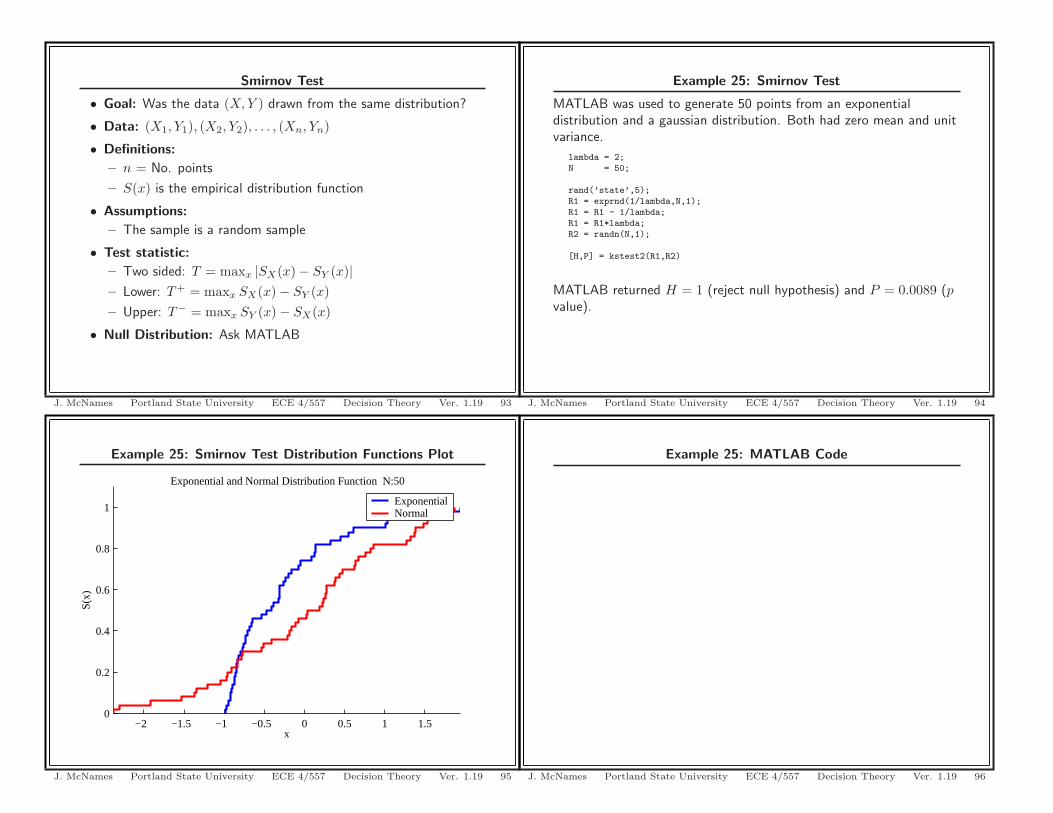
Example 25: Smirnov Test Distribution Functions Plot
−2 −1.5 −1 −0.5 0 0.5 1 1.50
0.2
0.4
0.6
0.8
1
x
S(x)
Exponential and Normal Distribution Function N:50
ExponentialNormal
J. McNames Portland State University ECE 4/557 Decision Theory Ver. 1.19 95
Smirnov Test
• Goal: Was the data (X, Y ) drawn from the same distribution?
• Data: (X1, Y1), (X2, Y2), . . . , (Xn, Yn)
• Definitions:
– n = No. points
– S(x) is the empirical distribution function
• Assumptions:
– The sample is a random sample
• Test statistic:
– Two sided: T = maxx |SX(x) − SY (x)|– Lower: T+ = maxx SX(x) − SY (x)– Upper: T− = maxx SY (x) − SX(x)
• Null Distribution: Ask MATLAB
J. McNames Portland State University ECE 4/557 Decision Theory Ver. 1.19 93
Example 25: MATLAB Code
J. McNames Portland State University ECE 4/557 Decision Theory Ver. 1.19 96
Example 25: Smirnov Test
MATLAB was used to generate 50 points from an exponentialdistribution and a gaussian distribution. Both had zero mean and unitvariance.
lambda = 2;N = 50;
rand(’state’,5);R1 = exprnd(1/lambda,N,1);R1 = R1 - 1/lambda;R1 = R1*lambda;R2 = randn(N,1);
[H,P] = kstest2(R1,R2)
MATLAB returned H = 1 (reject null hypothesis) and P = 0.0089 (pvalue).
J. McNames Portland State University ECE 4/557 Decision Theory Ver. 1.19 94

Tests for Normality
• See lillietest for testing against normal populations
• Also popular is the chi-squared goodness of fit test
J. McNames Portland State University ECE 4/557 Decision Theory Ver. 1.19 97