x11 time series decomposition and sampling errors - australian

Working Paper No. 93/2

X11 TIME SERIES DECOMPOSITION

AND SAMPLING ERRORS

Andrew Sutcliffe

December 1993

This Working Paper Series is intended to make the results of currentresearch within the ABS available to other interested parties. The aim is topresent accounts of ABS developments and research work or analysis of anexperimental nature so as to encourage discussion and comment.Views expressed in this paper are those of the author(s) and do notnecessarily represent those of the Australian Bureau of Statistics. Wherequoted or used, they should be attributed clearly to the author(s).

ABSTRACT

There is considerable interest in analysing the effect of sample design on time seriesdecomposition into components such as trend, seasonal and residual. One of the maindeficiencies in past analysis has been a lack of a realistic model of an officially used timeseries decomposition method. This paper demonstrates a realistic approximation for X11and shows how such a model can be used to analyse the effect of sample design on timeseries decomposition.

1

TIME SERIES DECOMPOSITION USING X11 AND SAMPLING ERRORS

1. Introduction.

There is considerable interest in the effects of sampling error on the components of timeseries decomposition, such as, the seasonally adjusted, trend and residual data. Forexample it is useful to have standard errors on the seasonally adjusted data, trend, seasonaland residual which represent the effects of the sampling process. An important question iswhat proportion of the observed variability in a time series is due to sampling error. Thenthere are design considerations, for example given a certain sample design andcharacteristics what is an "optimal" time series decomposition. One of the maindeficiencies in past analysis has been providing a realistic model of an officially used timeseries decomposition method. This paper demonstrates a realistic model for X11(Shiskinet al, 1967) and shows how such a model can be used to analyse the effect of samplingdesign on time series decomposition.

To give a appreciation of the complexity of the problem consider the simple time seriesmodel

1.1 y∼ = t∼ + s∼ + e∼

where

1.2 is the trendt∼

is the seasonals∼

is the residual/irregulare∼

It is reasonable to assume the residual contains the following components

1.3 e∼ = erw∼ + es∼ + ens∼

where

1.4 is the "real world" noiseerw∼

is the sampling errores∼

is the non-sampling errorens∼

However the following sources of error may apply to the "true" decomposition :

(i) The sampling error will affect the estimation of the trend, seasonal and "realworld" noise. The sampling error may also contain "trend like" and

seasonal behaviour.

(ii) The non-sampling error will affect the estimation of the trend, seasonal and"real world" noise. In addition the non-sampling error may well

contain trend and seasonal components itself.

2

(iii) Revision to the data will effect components to varying degrees.

(iv) The components at the end of the data will be revised as more data becomesavailable due to the X11 method. That is assuming the central filters

in X11 give the "true" components the estimates at the end of thedata will only be an approximation.

(v) It is assumed that X11 methodology can adequately estimate the trend, seasonal and residual.

(vi) It is assumed that other components such as trading-day, moving holidays,and abrupt changes in the level or seasonal pattern are adequatelyestimated when they exist in the data.

2. Model to analyse the effect of sampling error on time series decomposition.

The Australian Bureau of Statistics (ABS) has used the X11 method for all officiallyseasonally adjusted time series since 1967. Generally time series sample surveys haveerror estimates that are correlated. Hence the two main tools to enable an analysis of theeffect of sampling errors on a time series are a realistic model of X11 and a covariancematrix associated with the sample design.

3. A realistic model of X11.

3.1 Previous modelsYoung (1963) gave a basic linear approximation to X11. In general though this, and othersubsequent work has been inadequate to accurately represent X11 as used in practice.The main area's where the previous models have been inadequate are :-

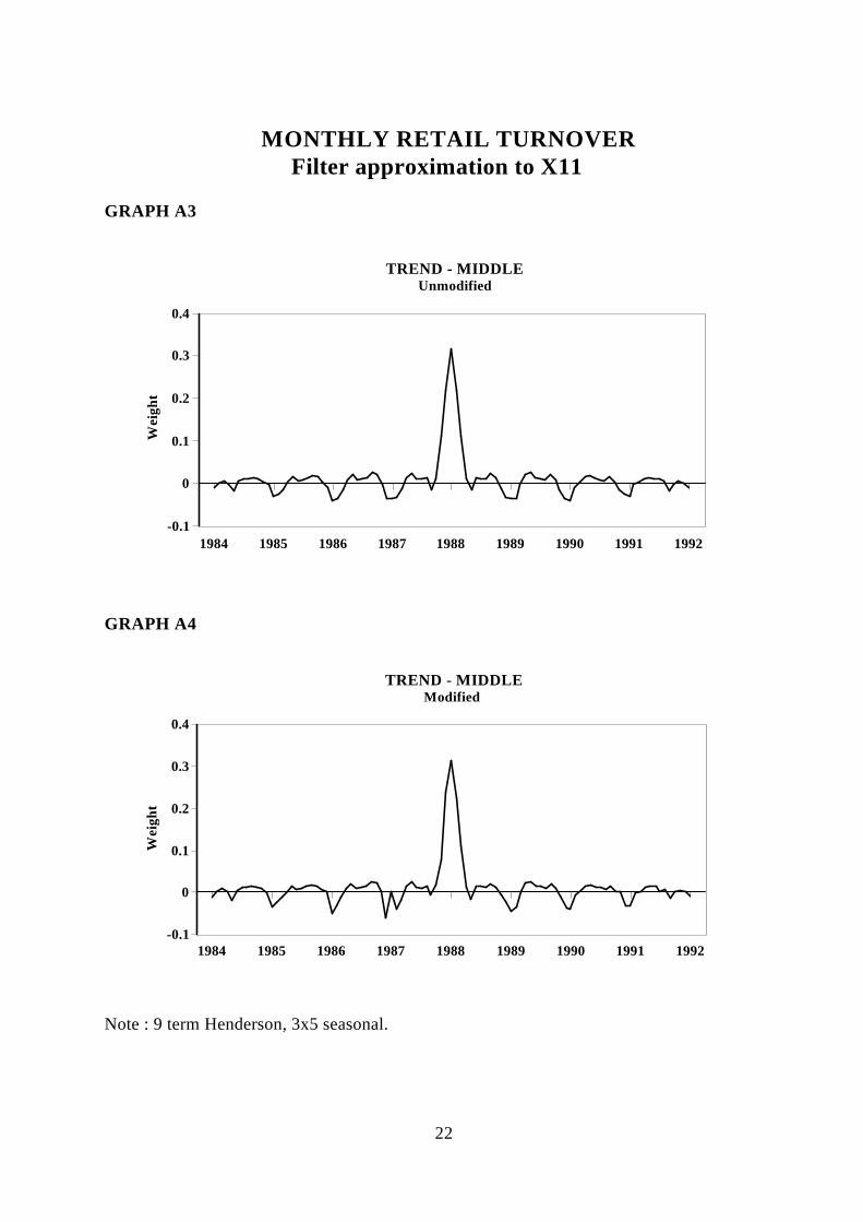
(i) Studies have mainly concentrated on the central filters used in X11. Theseare not representative of the actual filters used by X11 (for examplecompare graph A3 with A5).

(ii) In the main the standard options available in X11 have been used. All otheroptions have been ignored including the fact that X11 uses different

filters for short time series (e.g. 5 years long).

(iii) It is not recognised that logging the data and adjusting additively is not equivalent to the multiplicative option in X11 especially in terms of the arithmetic levels.

(iv) The modification for outliers used in X11 is usually completely ignored.

(v) Effects such as trading-day, moving holidays, trend breaks, seasonal breaksetc. have been ignored.

3

For example the often quoted paper by Cleveland et al. (1976), is clearly deficient on all ofthe above concerns. Other papers that are deficient in at least some of the considerationsabove include Hausman and Watson (1985), Maravall (1985), and Butter and Mourik(1990). A much more comprehensive treatment is given in the recently published workingpaper by Dagum, Chhab and Chiu (1993).

3.2 Other MethodsSome authors have assumed other theoretical models for the decomposition. These includeSABL,STL (Cleveland et al.) which use moving medians and local regressionrespectively, BSM (Maravall et al. 1985) a basic structural model , and STM(Butter andMourik, 1990) a structural model using a State Space representation and estimated usingthe Kalman filter. This approach ignores the fact that many major statistical organisationsare using X11. In addition these alternative models are still deficient with respect to someof the points listed above.

Professor James Durbin said in a speech in 1986 "...and a great deal of progress has beenmade in the theory of time series analysis. It would, therefore, have been natural to expectthat improvements in methods of seasonal adjustment would have taken place at a rapidrate, and that the techniques in daily use today would have been revolutionised comparedto the X11 method of twenty year ago. However this has not happened." Part of theproblem even today is that while many new structural models have been proposed andoffer promising alternatives to X11 they are not developed or tested to a form suitable fora large statistical organisation to decompose hundreds, or even thousands of time serieswith differing characteristics.

3.3 Non-iterative version of X11.

One of the design features of X11 is to provide an ad-hoc iterative procedure thatconverges to a relatively stable estimate quickly. A non-iterative procedure that gives verysimilar results to X11 is outlined below. A feature of this implementation is that a generalmatrix language (PROC IML in SAS) has been used. This has enabled compact code andall of the options available in X11 (and some that are not) to be included.

3.4. Notation3.4.1 n by 1 vectors where n is the length of the data

original datay∼

trendt∼

seasonals∼

residual/irregulare∼

weights(0 no modification, 1 fully modified)w∼

seasonally adjusted dataa∼

3.4.2 n by n matrices :A matrix to derive the trend from seasonally adjusted data. For example forT

a 7 term Henderson the matrix would look like:

4

T =

0.535 0.383 0.116 −0.034 0 . . . 00.289 0.410 0.294 0.061 −0.054 0 . . 00.034 0.275 0.399 0.287 0.058 −0.053 0 . 0

−0.059 0.059 0.294 0.412 0.294 0.059 −0.059 . 00 . . . . . . . .0 . . . . . . . .0 . . . . . . . .0 . . . . . . . .0 . . . . −0.034 0.116 0.383 0.535

3.4.3 A matrix to compute the seasonal factors from the detrended data.S1 For example a 3 by 5 moving average.

3.4.4 A matrix to correct for levels.. For example a 2 by 12 moving average.S2Let

3.4.5 S = (I − S2) ∗ S1

Then for a simple additive model

3.4.6 y∼ = t∼ + s∼ + e∼

we have three equations

3.4.7 t∼ = T ∗ (y∼ − s∼)s∼ = S ∗ (y∼ − t∼)e∼ = y∼ − t∼ − s∼

Hence

3.4.8 t∼ = T ∗ (y∼ − S ∗ (y∼ − t∼ ))(I − T ∗ S) ∗ t∼ = (T − T ∗ S) ∗ y∼

Providing that the inverse exists we have

3.4.9 t∼ = (I − T ∗ S)−1 ∗ (T − T ∗ S) ∗ y∼

Hence the component's and the adjusted data can be directly computed from .t∼ , s∼, e∼ a∼ y∼

3.4.10 wheret∼ = T ∗ y∼ T = (I − T ∗ S)−1 ∗ (T − T ∗ S)wheres∼ = S ∗ y∼ S = S − S ∗ Twheree∼ = E ∗ y∼ E = I − T − Swherea∼ = A ∗ y∼ A = (I − S)

3.5. Multiplicative adjustmentIf

5

3.5.1 y∼ = t∼ ∗ s∼ ∗ e∼

then logging 3.3.1 gives an additive model in logs

3.5.2 log(y∼) = log(t∼ ) + log(s∼) + log(e∼)

Hence estimates of the components are given by

3.5.3 t∼ = exp(T ∗ log(y∼))s∼ = exp(S ∗ log(y∼))e∼ = exp(E ∗ log(y∼))

Unfortunately this leads to geometric moving averages being applied. This means thatlevels are maintained in geometric rather than arithmetic terms (as say multiplicative X11does). It is interesting to note that the symmetric Henderson weights do have the propertythat the weights applied to logged data and then un-logged are very close to the weightsapplied directly to the un-logged data (because Henderson moving averages leavepolynomial trends of up to cubics unchanged). The end weights and the moving averagesused to obtain the seasonal factors from the de-trended data do not have this property.Hence, if a seasonal series is adjusted using multiplicative X11 and compared to the sameadjustment logging the data, applying an additive adjustment and then un-logging the dataa systematic bias is observed in say the trend levels. There are many ways to attempt tocorrect for this bias. A simple and effective way is to correct the seasonal factors obtainedwith the log additive model for multiplicative level bias.

That is

3.5.4 sbias∼ = exp(S ∗ log(y∼))s∼ = sbias∼/(S2 ∗ sbias∼))

3.6. Modifications for extremesAn important part of X11 is to deal with outliers. To accurately represent X11 (and toprovide good estimates of the components) outliers must be modified. A simple andeffective method is to use the concept of a weight applied to the data.

That is, let be a vector of weights to apply, where gives no modification andw∼ w(i) = 0 gives full modification, and gives partial modification. Then it can bew(i) = 1 0 < w(i) < 1

shown that the matrices to derive the trend, seasonal and residual can be modified to allowfor outliers as shown below.

Assuming have been computed as outlined above then they can be modified toT, S and Etake account of outliers as follows

3.6.1 E = (I − (I − E) ∗ diag(w∼))−1 ∗ ET = T ∗ (I − diag(w∼) ∗ E)S = S ∗ (I − diag(w∼) ∗ E)

6

The weights can be taken from X11 or directly computed using a method similar tow∼

X11. In theory the computation of the weights would need to be taken into account forstandard errors on the estimates. This has not been attempted in this paper.

Several alternative methods of handling outliers are currently being investigated. Theseinclude modifications of the form

3.6.2 y∼ − λ∼

where is of the formλ∼

3.6.3 where λ∼ = g ∗ (I + g ∗ E ∗ E)−1 ∗ E ∗ E ∗ y∼ 0 ≤ g < ∞

or with suitable G

3.6.4 λ∼ = g ∗ (I + g ∗ G ∗ E ∗ E ∗ G)−1 ∗ G ∗ E ∗ E ∗ y∼

One interesting application is the choice of to enable outliers to receive more smoothingGrather that being removed or reduced in the data.

3.7. Trading-day, moving holidays and other influencesOthers types of components such as trading-day, moving holidays and abrupt changes inthe level or seasonal pattern can be incorporated into the methodology outlined above.

For example letting be an n by k matrix where k is the number of parameters to beXestimated and appropriately formulated for trading-day (Young 1965) or movingXholidays. Then these components can be incorporated as

3.7.1 D = (I − H ∗ (I − E))−1 ∗ H ∗ E

where H = X ∗ (X ∗ X)−1 ∗ X .

The other components are modified as

3.7.2 T = T ∗ (I − D)S = S ∗ (I − D)E = I − T − S − D

3.8. Extensions to X11The basic X11 algorithm can easily be extended to include other models, for example it isa simple extension to allow for regression estimates of the trend and seasonal components.The residual component could be allowed to follow a moving average process(Box-Jenkins). For example for the basic model

3.8.1 y∼ = t∼ + s∼ + e∼

the residual could follow a moving average process of order 1e∼

7

3.8.2 where e(t) = ε(t) − θ ∗ ε(t − 1) ε~N(0, σ2)

letting

3.8.3 G =

1 0 0 0 . 0−θ 1 0 0 . 00 −θ 1 0 . 00 . . . . .. . . −θ 1 00 . 0 0 −θ 1

we have

3.8.4 ε∼ = (I − E ∗ (I − G))−1 ∗ E ∗ y∼

Hence could be estimated by least squares by minimising or with appropriateθ ε∼ ∗ ε∼modifications by maximum likelihood.

3.9. ImplementationThe vector and matrix formulation given above is ideally suited to Proc IML in SAS, andother matrix oriented packages. All computations have been done using IML. Thecomputations for the Henderson moving averages have been done using algorithms for thecentral and surrogate weights (used at the ends of the data) to make the method moregeneral.

As an example Australian Monthly Retail Turnover has been used. The data from the1992 annual re-analysis with the same prior correction factors has been used. The span ofthe analysis has been restricted to 7/83 to 6/92 due to the large amount of computermemory required.

The seasonal factors are computed using the above methodology from 7/83 to 6/92 and theforward factors computed using the same method as in X11. The adjusted series iscompared to the published figures (April 1993) in graph A1. The movements arecompared in Graph A2. For this example the differences are minor. Several other timeseries have been looked at with similar results. More comprehensive testing is envisagedin the future.

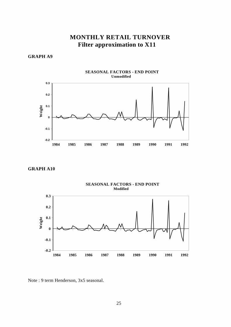
Graphs A3 to A14 shows the weights for some selected point in time for the trend,seasonal and irregular components. Some of the features are that the weighting patterns atthe ends of the data are completely different to those at the centre (e.g. compare A3 withA5). The modified weighting patterns may be similar to the unmodified in some cases,and different in others, depending on the weights and the location of the extremes (e.g.compare A7 and A8).

Graph A9 shows graphically for the case of a 9 term Henderson, 3x5 seasonal andTmodifications for extremes for the Monthly Retail Turnover data. The left hand axis is the

8

actual weights, the bottom axis is the time point at which the filter given by the right axisis applied.

While not shown in this paper the spectral properties of the filters outlined above can beextensively analysed using the gain and phase outputs of a linear filter.

4. A covariance matrix associated with the sample design.

The computation of the covariance matrix associated with the sampling design is mainly asampling problem. There seems to be three approaches possible. These are :

(i) Compute the whole covariance matrix directly using the sampling design. There would usually be computational difficulties in computing such

a matrix going back several years.

(ii) Find a model to estimate the covariances. This was the approach taken bySteel and De Mel (1987) for the Australian Labour Force Data where a"geometric decay" model is used.

(iii) Make up the covariance matrix using an educated guess for the model.

It should be noted that any covariance matrix used must be positive semi-definite to ensurezero or positive variances.

The analysis would be considerably complicated if the sampling error, non-sampling errorand "real world" error are correlated. There is also the somewhat philosophical problem oflooking at the "true" observed values as fixed, versus their own distribution, that is are thesample totals fixed or random variables. Given these tools the type of analysis that can beachieved is outlined below.

The basic theoretical framework is outlined in section 3. Ignoring a correction for levels,the components of a multiplicative time series analysis, with modification for extremes(using the modifications in 3.4), is given by

4.1 t∼ = exp(T ∗ log(y∼))s∼ = exp(S ∗ log(y∼))e∼ = exp(E ∗ log(y∼))

5. Additive verses multiplicative standard errors.

The published standard errors are usually given as an additive standard error. Given themultiplicative option in X11 is almost always used this means that the basic model is givenby

5.1 y∼ = t∼ ∗ s∼ ∗ erw∼ ∗ ens∼ + es∼

9

This presents some problems, namely:

(i) Logging the data does not give a model which is easy to analyse.

(ii) Such a model cannot be totally reasonable since it implies negative valuesare possible in data that cannot be usually negative.

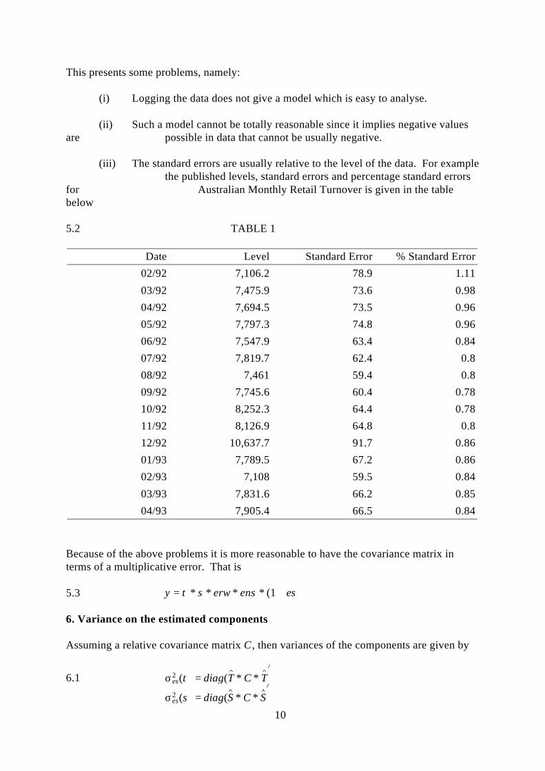
(iii) The standard errors are usually relative to the level of the data. For examplethe published levels, standard errors and percentage standard errors

for Australian Monthly Retail Turnover is given in the tablebelow

5.2 TABLE 1

Date Level Standard Error % Standard Error02/92 7,106.2 78.9 1.1103/92 7,475.9 73.6 0.9804/92 7,694.5 73.5 0.9605/92 7,797.3 74.8 0.9606/92 7,547.9 63.4 0.8407/92 7,819.7 62.4 0.808/92 7,461 59.4 0.809/92 7,745.6 60.4 0.7810/92 8,252.3 64.4 0.7811/92 8,126.9 64.8 0.812/92 10,637.7 91.7 0.8601/93 7,789.5 67.2 0.8602/93 7,108 59.5 0.8403/93 7,831.6 66.2 0.8504/93 7,905.4 66.5 0.84

Because of the above problems it is more reasonable to have the covariance matrix interms of a multiplicative error. That is

5.3 y∼ = t∼ ∗ s∼ ∗ erw∼ ∗ ens∼ ∗ (1 + es∼)

6. Variance on the estimated components.

Assuming a relative covariance matrix , then variances of the components are given byC

6.1 σes2 (t∼ ) = diag(T ∗ C ∗ T )

σes2 (s∼) = diag(S ∗ C ∗ S )

10

σes2 (e∼) = diag(E ∗ C ∗ E )

Hence 95 per cent confidence bounds (assuming 2 sigma is 95%) for the components are±given by

6.2 t∼ ∗ (1 ± 2 ∗ σes(t∼ ))

s∼ ∗ (1 ± 2 ∗ σes(s∼))e∼ ∗ (1 ± 2 ∗ σes(e∼))

From these formulas additive errors can be numerically computed. It should be noted that these estimates are highly correlated, and hence cannot be used to give simultaneousconfidence bounds on several time points. In addition these formulas will only provideestimates of the uncertainly due to the sampling error.

To give an example Monthly Retail Turnover data has been analysed. It should be notedthat this analysis is for demonstration purposes only, and is not necessarily realistic. Inpractice the covariance matrix associated with the sample design would include explicitallowance for the rotation used, sample redesign and other known sampling designcharacteristics. The sample design area of the ABS is currently researching suchcovariance matrices for the ABS sample surveys.

An examination of table 1 above and the standard errors on the movements given in thepublication a standard error of about 1 per cent and a high correlation between successivetime points might be a reasonable model for the covariance matrix. A possible modelmight be an AR(1) model of the form

6.3 where iid with variance es t = ρ ∗ es t−1 + ε t ε t σ2

it can be shown that this has the covariance matrix

6.4 σ2

1−ρ2

1 ρ ρ2 . . ρn−1

ρ 1 ρ . . ρn−2

. . . . . .

. . . . . .ρn−2 . . ρ 1 ρρn−1 . . ρ2 ρ 1

Hence letting and gives a 1 per cent standard error andρ = 0.8 σ2 = 0.0001 ∗ (1 − 0.82)correlation at lag 1 of 0.8 (an alternative model might have been a MA(1)).

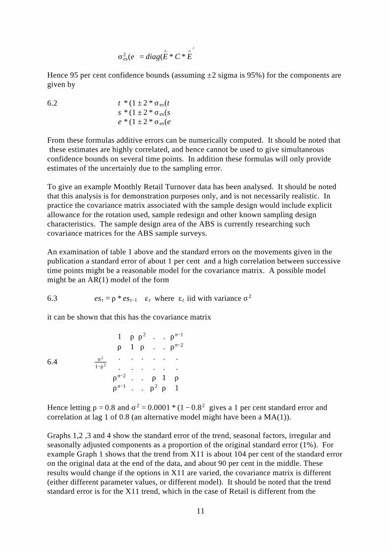
Graphs 1,2 ,3 and 4 show the standard error of the trend, seasonal factors, irregular andseasonally adjusted components as a proportion of the original standard error (1%). Forexample Graph 1 shows that the trend from X11 is about 104 per cent of the standard erroron the original data at the end of the data, and about 90 per cent in the middle. Theseresults would change if the options in X11 are varied, the covariance matrix is different(either different parameter values, or different model). It should be noted that the trendstandard error is for the X11 trend, which in the case of Retail is different from the

11

published trend. This is because ABS currently uses a 9 term Henderson for the seasonaladjustment, while the published trend is uses a 13 term Henderson, and no allowance ismade for outliers in the published trend.

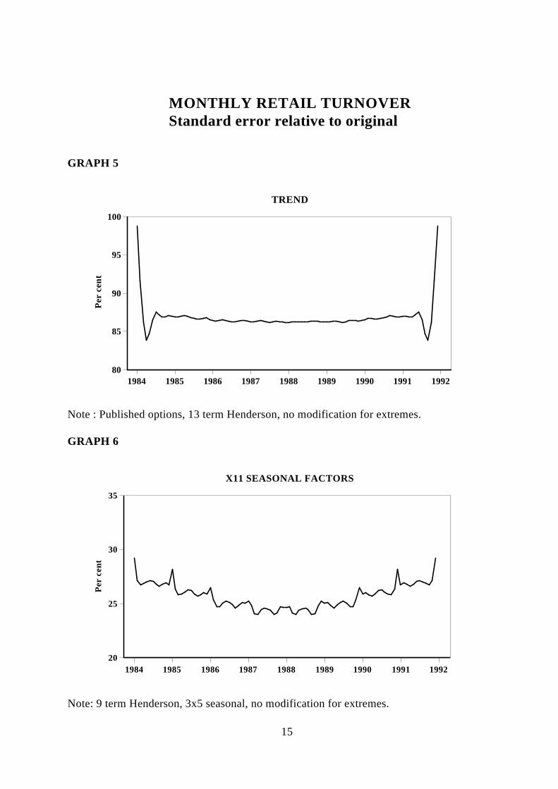
It is relatively straightforward to modify the procedure to allow for these differences. Theapproximate standard error of the published trend as a proportion of the original standarderror is shown in graph 5. If the proportions of the trend in graph 1 and graph 5 arecompared it will be noticed that it is lower in graph 5 (NB 13 vs 9 Henderson). Howeverthis does not however imply that estimation of the trend without modifications forextremes is superior. There are two competing factors in estimating the trend (or any othercomponent) "bias" and "variance". That is the trend produced without modifications forextremes may have a lower variance but be also very biased in producing what is deemeda reasonable trend.

A similar situation is faced at the end of the data. It has been noticed for some time seriesthat the trend produced at the end of the data seems to be biased when compared to thefinal trend. Such bias could be eliminated by applying the same criteria that are used tocompute the central Henderson weights at the end of the data. The result would be a muchhigher variance on the trend at the end of the data.

Comparing these results with the work of Steel and De Mel (op. at.) shows that while thereare broad similarities in the magnitude, it is clear that there is considerably morecomplexity in the filters actually used in X11 to obtain the components. Some interestingfeatures are the pronounced rises in the early years of the proportion for the seasonalfactors. This is due to a predominance of full modification for outliers in those months(compare with graph 6).

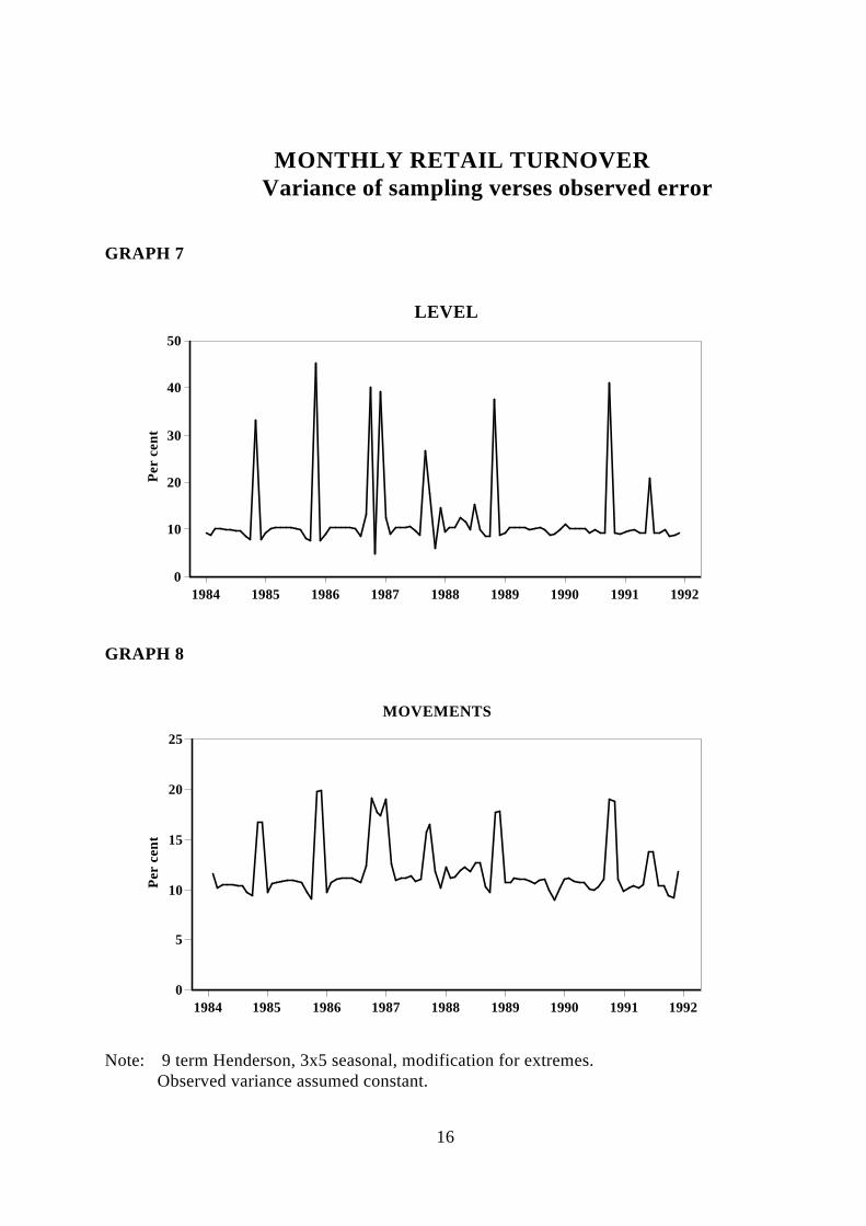
The variability of the residual due to the sampling process can be compared with theestimate of variance for the observed residual. This includes "real world" error, samplingerror and non-sampling error, and (assuming a constant variance), is given by :

6.5 σe2 = 1

n Σ t=1n (e t − 1)2

Hence the percentage of volatility of the levels of Monthly Retail Turnover due to thesampling process is approximated by

6.6 100 ∗ σes2 (e∼)

σe2(e∼)

Graph 7 shows this percentage over time. In practice, the "real world" variance is almostcertainly changing over time and there is plenty of empirical evidence that it is seasonal.It is a moot point whether the proportion should be to the actual observed residual or theresidual modified for outliers. In the latter case the proportion would be much higher.

12

MONTHLY RETAIL TURNOVERStandard error relative to original

GRAPH 1

1984 1985 1986 1987 1988 1989 1990 1991 1992 80

85

90

95

100

105

110

Per

cen

t

X11 TREND

GRAPH 2

1984 1985 1986 1987 1988 1989 1990 1991 1992 20

25

30

35

Per

cen

t

X11 SEASONAL FACTORS

Note: 9 term Henderson, 3x5 seasonal, modification for extremes.

13


GRAPH 3

1984 1985 1986 1987 1988 1989 1990 1991 1992 0

10

20

30

40

50

60

70

Per

cen

t

X11 RESIDUAL

GRAPH 4

1984 1985 1986 1987 1988 1989 1990 1991 1992 90

95

100

105

Per

cen

t

X11 ADJUSTED

Note: 9 term Henderson, 3x5 seasonal, modification for extremes.

14


GRAPH 5

1984 1985 1986 1987 1988 1989 1990 1991 1992 80

85

90

95

100

Per

cen

t

TREND

Note : Published options, 13 term Henderson, no modification for extremes.

GRAPH 6

1984 1985 1986 1987 1988 1989 1990 1991 1992 20

25

30

35

Per

cen

t

X11 SEASONAL FACTORS

Note: 9 term Henderson, 3x5 seasonal, no modification for extremes.

15

MONTHLY RETAIL TURNOVERVariance of sampling verses observed error

GRAPH 7

1984 1985 1986 1987 1988 1989 1990 1991 1992 0

10

20

30

40

50

Per

cen

t

LEVEL

GRAPH 8

1984 1985 1986 1987 1988 1989 1990 1991 1992 0

5

10

15

20

25

Per

cen

t

MOVEMENTS

Note: 9 term Henderson, 3x5 seasonal, modification for extremes.Observed variance assumed constant.

16

7. Variance of the movements.

These are estimated in a similar fashion to that of the levels shown in section 4. In thiscase define

7.1 where , the shift operator, shifts the rows of a matrixD t = T − BT Bdown one.

Ds = S − BSDe = E − BE

Then the approximate variances on the movements due to the sampling process is given by

7.2 σes2 ((t∼ − Bt∼)/Bt∼ ) = diag(D t ∗ C ∗ D t )

σes2 ((s∼ − Bs∼)/Bs∼) = diag(Ds ∗ C ∗ Ds )

σes2 ((e∼ − Be∼)/Be∼) = diag(De ∗ C ∗ De )

Again, the variance of the change in the irregular component can be compared with theestimated variance of the observed change in the residual. This is given by

7.3 σe2((e∼ − Be∼)/Be∼) = 1

n−1 Σ t=2n ( et

et−1− 1)2

Hence the percentage of volatility of the movements of Monthly Retail Turnover due tothe sampling process is approximately given by

7.4 100 ∗ σes2 ((e∼−Be∼)/Be∼)

σe2((e∼−Be∼)/Be∼)

Graph 8 shows this percentage over time.

8. Can better estimates of the "real" data be computed?

There are several approaches that can be used to provide better estimates of the "real" data.Unfortunately because there are so many sources of error any method proposed canalways be criticised because of the assumptions used.

One approach is to use spectral analysis. For example if it could be ascertained, eitherwith prior knowledge or empirical investigation, that the contribution of the variance dueto sampling error was concentrated in a certain bandwidth and the "real world" andnon-sampling error in a different bandwidth, then an appropriate filter could be designedusing spectral analysis to remove/dampen the sampling error and leave the other errorunchanged. More formally if the model for the observed data is

8.1 y∼ = t∼ + s∼ + es∼ + er∼

where

17

8.2 is the sampling error andes∼

is the rest of the error.er∼

Then if one could find a filtering matrix such thatF

8.3 er∼ = F ∗ (es∼ + er∼) + ε∼

then it can be shown that a better estimate of the original data is given by

8.4 y∼b = I −

E + F ∗ (I − E)

−1∗ E ∗ (I − F)

∗ y∼

8.5 = R ∗ y∼

There are several ways a suitable matrix could be estimated. For example, if theFsampling error is assumed to follow an autoregressive model then it can be written as

8.6 G ∗ es∼ = ε∼

Then if depended on parameters they could be estimated by minimisingF

8.7 y∼ ∗ (G ∗ R) ∗ (G ∗ R) ∗ y∼

9. Sample design using time series characteristics.

If it is required to have an "optimal" sample allocation with respect to the decomposeddata then clearly time series characteristics of the data must be taken into account. Forexample Australian Monthly Retail Turnover has allocation goals of minimising standarderrors on movement and level for the original data. Generally if estimating the change inlevel between two time periods estimates of maximum precision are obtained by retainingthe same sample on both occasions. For average or total values over a number of surveysnon-overlapping units are selected. Clearly the trend level and movements are a weightedaverage of several survey values. If the goal was for a optimal sample for the trendcomponent from the decomposition then the sample design/allocation may well bedifferent.

In the example for Australian Monthly Retail Turnover the observed variance wasassumed to be constant. In practice the variance may well be changing over time and isoften observed to be seasonal.

It is possible to compute a time varying variance in a similar manner to that of the levels.For example, using a 5 year moving average and constant seasonality a model for thevariance might be ( where is derived in a similar way to that of the levels in section 3)V

9.1 σ∼2(e∼) = V ∗ e∼2

where9.2 e∼ = E ∗ y∼

18

In which case 9.1, could be used to assist in deriving an optimal sample allocation.

It should also be pointed out that autocorrelation in the residual due to sample design error(if strong enough) could be used to determine optimal filters for the time series

decomposition.

10. Conclusions.

This paper demonstrates that a realistic approximation of X11, the widely used time seriesdecomposition package, is possible. This provides a tool to allow extensive analysis ofsample design and characteristics on time series decomposition. In particular, given amodel for the covariance matrix of the sample design, and making certain assumptions thepaper shows thatstandard errors can be computed on components such as trend, seasonal and residual at alltime points, and the proportion of variance due to sampling error can be estimated.

This paper only outlines the tools required for the analysis and further work needs to becompleted on practical applications for individual surveys.

Currently, sampling design concentrates only on the original data. Given that theAustralian Bureau of Statistics is giving more emphasis on the "trend" estimates it is not atall obvious that an "optimal" sample design for the original data will be "optimal" for thetrend as estimated by the Australian Bureau of Statistics. This is clearly an area wherefurther work is required to integrate the sample design and decomposition process.

19

REFERENCES

ABS Catalogue No 8501.0, Retail Trade Australia, April (1993).

Box G.E.P., Jenkins G.M., Time series analysis forecasting and control, 2nd ed, SanFrancisco, Holden Day, (1976).

Butter F.A.G., Mourik T.J., Seasonal adjustment using structural time series models: Anapplication and comparison with census X-11 method, Journal of Business and EconomicStatistics, Vol 8, No 4, October (1990), 385-393.

Cleveland W.P., Tiao G.C., Decomposition of seasonal time series: A model for the censusX-11 program, Journal of the American Statistical Association, Vol 71, No 355,September (1976), 581-587.

Cleveland R.B., Cleveland W.S., McRae J., Terpenning I., STL: A Seasonal-Trenddecomposition procedure based on Loess, Journal of Official Statistics, Vol 6, No 1,(1990), 3-73.

Dagum E.B., Chhab N., Chiu K., Linear filters of the X11-ARIMA method, StatisticsCanada, Working Paper No BSMD-93-008E, (1993).

Hausman J.A., Watson M.W., Errors in variables and seasonal adjustment procedures,Journal of the American Statistical Association, Vol 80, No 391, (1985), 531-539.

Maravall S., Pierce D.A., On structural time series models and the characterisation ofcomponents, Journal of Business and Economic Statistics, 3, (1985), 350-355.

SAS Institute Inc., SAS System Version 5, Cary, NC, SAS Institute Inc, (1985).

Shiskin J., Young A.H., Musgrave J.C., The X11 variant of the Census Method II:Seasonal adjustment program, Technical Paper 15, US Department of Commerce, Bureauof the Census, (1967).

Steel D.G., de Mel R.G., The contribution of sampling error to the variability of statisticalseries, Unpublished, Australian Bureau of Statistics, (1987).

Young A.H., Linear approximation to the Census and BLS seasonal adjustment methods,JASA, (1968), 445-471.

Young A., Estimating trading-day variation in monthly economic time series, TechnicalPaper No 12, US Department of Commerce, Bureau of Census, (1965).

20

COMPARISON OF PUBLISHED SEASONAL ADJUSTMENTto APPROXIMATION OF X11

GRAPH A1

Feb 92 May 92 Aug 92 Nov 92 Feb 93 7700

7800

7900

8000

8100

8200

$Mill

ion

Published non X11

Monthly Retail Turnover

GRAPH A2

Feb 92 May 92 Aug 92 Nov 92 Feb 93 -4-3-2-1012345

Per

cen

t cha

nge

Published non X11

Monthly Retail Turnover

21

MONTHLY RETAIL TURNOVER Filter approximation to X11

GRAPH A3

1984 1985 1986 1987 1988 1989 1990 1991 1992 -0.1

0

0.1

0.2

0.3

0.4

Wei

ght

TREND - MIDDLEUnmodified

GRAPH A4

1984 1985 1986 1987 1988 1989 1990 1991 1992 -0.1

0

0.1

0.2

0.3

0.4

Wei

ght

TREND - MIDDLEModified

Note : 9 term Henderson, 3x5 seasonal.

22


GRAPH A5

1984 1985 1986 1987 1988 1989 1990 1991 1992 -0.2

-0.1

0

0.1

0.2

0.3

0.4

0.5

0.6

Wei

ght

TREND - ENDPOINTUnmodified

GRAPH A6

1984 1985 1986 1987 1988 1989 1990 1991 1992 -0.3

-0.2

-0.1

0

0.1

0.2

0.3

0.4

0.5

0.6

Wei

ght

TREND - ENDPOINTModified


23


GRAPH A7

1984 1985 1986 1987 1988 1989 1990 1991 1992 -0.05

0

0.05

0.1

0.15

0.2

Wei

ght

SEASONAL FACTORS - MIDDLEUnmodified

GRAPH A8

1984 1985 1986 1987 1988 1989 1990 1991 1992 -0.1

-0.05

0

0.05

0.1

0.15

0.2

0.25

Wei

ght

SEASONAL FACTORS - MIDDLEModified


24


GRAPH A9

1984 1985 1986 1987 1988 1989 1990 1991 1992 -0.2

-0.1

0

0.1

0.2

0.3

Wei

ght

SEASONAL FACTORS - END POINTUnmodified

GRAPH A10

1984 1985 1986 1987 1988 1989 1990 1991 1992 -0.2

-0.1

0

0.1

0.2

0.3

Wei

ght

SEASONAL FACTORS - END POINTModified


25


GRAPH A11

1984 1985 1986 1987 1988 1989 1990 1991 1992 -0.3

-0.2

-0.1

0

0.1

0.2

0.3

0.4

0.5

0.6

Wei

ght

RESIDUAL - MIDDLEUnmodified

GRAPH A12

1984 1985 1986 1987 1988 1989 1990 1991 1992 -0.3

-0.2

-0.1

0

0.1

0.2

0.3

0.4

0.5

0.6

Wei

ght

RESIDUAL - MIDDLEModified


26


GRAPH A13

1984 1985 1986 1987 1988 1989 1990 1991 1992 -0.4

-0.3

-0.2

-0.1

0

0.1

0.2

0.3

0.4

Wei

ght

RESIDUAL - END POINTUnmodified

GRAPH A14

1984 1985 1986 1987 1988 1989 1990 1991 1992 -0.4

-0.3

-0.2

-0.1

0

0.1

0.2

0.3

0.4

Wei

ght

RESIDUAL - END POINTModified


27

Contents

Abstract....................................................................................... 1 1. Introduction............................................................................ 2 2. Model to analyse the effect of sampling error on time series.... 3 3. A realistic model of X11.......................................................... 3

3.1. Previous models........................................................ 33.2. Other methods........................................................... 43.3. Non-iterative version of X11..................................... 43.4. Notation.................................................................... 43.5. Multiplicative adjustment........................................... 53.6. Modifications for extremes........................................ 63.7. Trading-day, moving holidays and other influences.... 73.8. Extensions to X11..................................................... 73.9. Implementation......................................................... 8

4. A covariance matrix associated with the sample design............ 9 5. Additive versus multiplicative standard errors......................... 9 6. Variance on the estimated components.................................... 10 7. Variance on the movements.................................................... 17 8. Can better estimates of the "real" data be computed?............... 17 9. Sample design using time series characteristics........................1810. Conclusions........................................................................... 1911. References............................................................................. 2012. Appendices............................................................................. 21

INQUIRIES

For further information about the contents of this Working Paper, please contactthe author:

Andrew Sutcliffe - Canberra (06) 252 7646 (telephone) or (06) 253 1093(facsimile).

For information about the Working Papers in Econometrics and Applied Statistics,please contact the Managing Editor, Geneviève Knight on Canberra(06) 252 6427(telephone) or (06) 253 1093 (facsimile), or write care of Econometric Analysis

x11 time series decomposition and sampling errors - australian

Documents