xml data transformation and integration — a schema - citeseer
TRANSCRIPT

XML Data Transformation and
Integration — A Schema
Transformation Approach
Lucas Zamboulis
November 2009
A Dissertation Submitted to
Birkbeck College, University of London
in Partial Fulfillment of the Requirements
for the Degree of Doctor of Philosophy
School of Computer Science & Information Systems
Birkbeck College
University of London

2
Declaration
This thesis is the result of my own work, except where explicitly acknowledged
in the text.
Lucas Zamboulis
November 4, 2009

Abstract
The process of transforming and integrating XML data involves resolving the
syntactic, semantic and schematic heterogeneities that the data sources present.
Moreover, there are a number of different application settings in which such a
process could take place, such as centralised or peer-to-peer settings, each of
which needs to be considered separately.
In this thesis, we investigate the problem of data transformation and integra-
tion for XML data sources. This data format presents a number of challenges
that require XML-specific solutions: a schema is not required for an XML data
source, and if one exists, it may be expressed in a number of different XML
schema types; also, resolving schematic heterogeneity is not straightforward due
to the hierarchical nature of XML data.
We propose a modular approach, based on schema transformations, that han-
dles the distinct problems of syntactic, semantic and schematic heterogeneity of
XML data. We handle the problem of syntactic heterogeneity of XML schema
types by introducing a new, automatically derivable schema type for XML data
sources, designed specifically for the purposes of XML data transformation and
integration. We show how semantic heterogeneity can be handled in our ap-
proach using existing methods, and we also propose a new semi-automatic method
for resolving semantic heterogeneity using mappings to ontologies as a ‘seman-
tic bridge’. We then present a new schema restructuring method that handles
schematic heterogeneity automatically, assuming that semantic heterogeneity is-
sues have been resolved.
The contribution of this thesis is the investigation of the problem of XML data
3

transformation and integration for all types of heterogeneity and in a variety of
application settings. We propose a modular approach to overcome the challenges
encountered and provide a number of automatic and semi-automatic techniques.
We show how our approach can be applied in different application settings and
we discuss the effectiveness and performance of our techniques via a number of
synthetic and real XML data transformation and integration scenarios.
4

To my parents
5

Acknowledgements
I am deeply grateful to my supervisors, Alexandra Poulovassilis and Nigel Martin,
for their continued support, their patient guidance and their faith in my work
throughout these years.
Many thanks are due to my colleagues at Birkbeck, Imperial and UCL for their
input, collaboration and numerous stimulating discussions. I would particularly
like to thank Rajesh Pampapathi, Michael Zoumboulakis, George Papamarkos,
George Roussos and Helge Gillmeister for their help and friendship — as well as
for the pints of cider after work.
Special thanks are due to Athena Vakali, Nikos Lorentzos and Yannis Manolo-
poulos, without whose help and support I would not have started this Ph.D. in
the first place.
Finally, my warmest thanks go to my family and friends for their love and
encouragement throughout this period and every other period. I would have never
finished this work without their support, and so this thesis is dedicated to them.
6

Contents
Abstract 3
Acknowledgements 6
1 Introduction 18
1.1 Introduction . . . . . . . . . . . . . . . . . . . . . . . . . . . . . . 18
1.2 Data Sharing . . . . . . . . . . . . . . . . . . . . . . . . . . . . . 19
1.2.1 Data Sharing Scenarios . . . . . . . . . . . . . . . . . . . . 19
1.2.2 Data Sharing Processes . . . . . . . . . . . . . . . . . . . . 20
1.3 Motivation and Contributions . . . . . . . . . . . . . . . . . . . . 21
1.4 Thesis Outline . . . . . . . . . . . . . . . . . . . . . . . . . . . . . 24
2 Review of Related Work on Data Transformation and Integra-
tion 25
2.1 Introduction . . . . . . . . . . . . . . . . . . . . . . . . . . . . . . 25
2.2 Heterogeneity Classification . . . . . . . . . . . . . . . . . . . . . 25
2.3 Data Transformation and Integration . . . . . . . . . . . . . . . . 27
2.3.1 Data Integration Approaches . . . . . . . . . . . . . . . . 27
2.3.2 Data Integration Strategies . . . . . . . . . . . . . . . . . 28
2.3.3 Schema Matching and Mapping . . . . . . . . . . . . . . . 29
2.3.4 Model Management . . . . . . . . . . . . . . . . . . . . . . 34
2.3.5 Peer-to-Peer Data Management . . . . . . . . . . . . . . . 36
2.4 XML Data Transformation and Integration . . . . . . . . . . . . . 37
2.4.1 XML and Related Technologies . . . . . . . . . . . . . . . 37
7

2.4.2 Schema Extraction . . . . . . . . . . . . . . . . . . . . . . 41
2.4.3 XML Schema Matching and Mapping . . . . . . . . . . . . 43
2.4.4 Publishing Relational Data as XML . . . . . . . . . . . . . 43
2.4.5 XML Schema and Data Integration . . . . . . . . . . . . . 44
2.4.6 XML Schema and Data Transformation . . . . . . . . . . . 49
2.4.7 Using Ontologies for Semantic Enrichment . . . . . . . . . 53
2.5 Discussion . . . . . . . . . . . . . . . . . . . . . . . . . . . . . . . 55
3 Overview of AutoMed 57
3.1 Introduction . . . . . . . . . . . . . . . . . . . . . . . . . . . . . . 57
3.2 The AutoMed Framework . . . . . . . . . . . . . . . . . . . . . . 57
3.2.1 The Both-As-View Data Integration Approach . . . . . . . 57
3.2.2 The HDM Data Model . . . . . . . . . . . . . . . . . . . . 58
3.2.3 Representing a Simple Relational Model . . . . . . . . . . 61
3.2.4 The IQL Query Language . . . . . . . . . . . . . . . . . . 61
3.2.5 AutoMed Transformation Pathways . . . . . . . . . . . . . 64
3.2.6 Query Processing . . . . . . . . . . . . . . . . . . . . . . . 67
3.2.7 The AutoMed Software Architecture . . . . . . . . . . . . 72
3.3 Using AutoMed for XML Data Sharing . . . . . . . . . . . . . . . 76
3.4 Summary . . . . . . . . . . . . . . . . . . . . . . . . . . . . . . . 78
4 XML Schema and Data Transformation and Integration 79
4.1 Introduction . . . . . . . . . . . . . . . . . . . . . . . . . . . . . . 79
4.2 A Schema Type for XML Data Sources . . . . . . . . . . . . . . . 80
4.2.1 Desirable XML Schema Characteristics in Transformation/
Integration Settings . . . . . . . . . . . . . . . . . . . . . . 80
4.2.2 Existing Schema Types for XML Data Sources . . . . . . . 81
4.2.3 XML DataSource Schema (XMLDSS) . . . . . . . . . . . . 84
4.2.4 XMLDSS Generation . . . . . . . . . . . . . . . . . . . . . 89
4.3 Overview of our XML Data Transformation/ Integration Approach 99
4.3.1 Schema Transformation Phase . . . . . . . . . . . . . . . . 99
4.3.2 Schema Conformance Phase . . . . . . . . . . . . . . . . . 109
8

4.4 Querying and Materialisation . . . . . . . . . . . . . . . . . . . . 110
4.4.1 Querying an XMLDSS Schema . . . . . . . . . . . . . . . 111
4.4.2 Materialising an XMLDSS Schema Using AutoMed . . . . 115
4.4.3 Materialising an XMLDSS Schema Using XQuery . . . . . 118
4.5 Summary . . . . . . . . . . . . . . . . . . . . . . . . . . . . . . . 119
5 Schema and Data Transformation and Integration 122
5.1 Introduction . . . . . . . . . . . . . . . . . . . . . . . . . . . . . . 122
5.2 Running Example for this Chapter . . . . . . . . . . . . . . . . . 123
5.3 Schema Conformance Via Schema Matching . . . . . . . . . . . . 126
5.4 Schema Restructuring Algorithm . . . . . . . . . . . . . . . . . . 130
5.4.1 Initialisation . . . . . . . . . . . . . . . . . . . . . . . . . . 131
5.4.2 Phase I - Handling Missing Elements . . . . . . . . . . . . 133
5.4.3 Phase II - Restructuring . . . . . . . . . . . . . . . . . . . 146
5.4.4 Correctness of the SRA . . . . . . . . . . . . . . . . . . . . 156
5.4.5 Complexity Analysis of the SRA . . . . . . . . . . . . . . . 158
5.5 Schema Integration Algorithms . . . . . . . . . . . . . . . . . . . 162
5.6 Discussion . . . . . . . . . . . . . . . . . . . . . . . . . . . . . . . 166
6 Extending the Approach Using Subtyping Information 168
6.1 Introduction . . . . . . . . . . . . . . . . . . . . . . . . . . . . . . 168
6.2 Running Example for this Chapter . . . . . . . . . . . . . . . . . 169
6.3 Representing Ontologies in AutoMed . . . . . . . . . . . . . . . . 171
6.4 Schema Conformance Using Ontologies . . . . . . . . . . . . . . . 174
6.4.1 XMLDSS-to-Ontology Correspondences . . . . . . . . . . . 174
6.4.2 XMLDSS-to-Ontology Conformance . . . . . . . . . . . . . 178
6.4.3 Schema Conformance Using Multiple Ontologies . . . . . . 183
6.5 Extended Schema Restructuring Algorithm . . . . . . . . . . . . . 185
6.5.1 Initialisation . . . . . . . . . . . . . . . . . . . . . . . . . . 187
6.5.2 Subtyping Phase . . . . . . . . . . . . . . . . . . . . . . . 190
6.5.3 Applying the Subtyping Phase . . . . . . . . . . . . . . . . 197
6.5.4 Applying Phase I and Phase II . . . . . . . . . . . . . . . 199
9

6.5.5 Discussion . . . . . . . . . . . . . . . . . . . . . . . . . . . 203
6.6 Summary . . . . . . . . . . . . . . . . . . . . . . . . . . . . . . . 203
7 Transformation and Integration of Real-World Data 205
7.1 Overview . . . . . . . . . . . . . . . . . . . . . . . . . . . . . . . . 205
7.2 Integration of Heterogeneous Data Sources
Using an XML Layer . . . . . . . . . . . . . . . . . . . . . . . . . 207
7.2.1 The BioMap Setting . . . . . . . . . . . . . . . . . . . . . 207
7.2.2 The Integration Process . . . . . . . . . . . . . . . . . . . 209
7.2.3 Implementation and Results . . . . . . . . . . . . . . . . . 215
7.3 XML Data Transformation and Materialisation . . . . . . . . . . 216
7.3.1 The Crime Informatics Setting . . . . . . . . . . . . . . . . 216
7.3.2 XMLDSS Schema Extraction . . . . . . . . . . . . . . . . 217
7.3.3 Schema Conformance . . . . . . . . . . . . . . . . . . . . . 219
7.3.4 Schema Restructuring . . . . . . . . . . . . . . . . . . . . 220
7.3.5 Schema Materialisation . . . . . . . . . . . . . . . . . . . . 221
7.4 Service Reconciliation Using A Single Ontology . . . . . . . . . . 222
7.4.1 Bioinformatics Service Reconciliation . . . . . . . . . . . . 222
7.4.2 Related Work in Service Reconciliation . . . . . . . . . . . 224
7.4.3 Our Service Reconciliation Approach . . . . . . . . . . . . 225
7.4.4 Case Study Using A Single Ontology . . . . . . . . . . . . 228
7.5 Service Reconciliation Using Multiple Ontologies . . . . . . . . . . 234
7.5.1 e-Learning Service Reconciliation . . . . . . . . . . . . . . 234
7.5.2 Transforming Ontologies using AutoMed . . . . . . . . . . 236
7.5.3 XML Data Source Enrichment . . . . . . . . . . . . . . . . 239
7.5.4 Ontology-Assisted Schema and Data Transformation . . . 240
7.6 Discussion . . . . . . . . . . . . . . . . . . . . . . . . . . . . . . . 243
8 Conclusions and Future Work 245
A BAV Pathway Generation Using PathGen 251
A.1 PathGen Input XML Format . . . . . . . . . . . . . . . . . . . . 251
10

A.2 Using Correspondences with PathGen . . . . . . . . . . . . . . . . 253
A.2.1 Correspondences XML Format . . . . . . . . . . . . . . . . 253
A.2.2 Transformation of a Set of Correspondences to the PathGen
Input XML Format . . . . . . . . . . . . . . . . . . . . . . 256
A.2.3 Application of PathGen on the Converted Sets of Corre-
spondences . . . . . . . . . . . . . . . . . . . . . . . . . . 260
B Correctness of the Schema Restructuring Algorithm 264
B.1 Introduction . . . . . . . . . . . . . . . . . . . . . . . . . . . . . . 264
B.2 Correctness Study . . . . . . . . . . . . . . . . . . . . . . . . . . . 267
B.2.1 Ancestor Case . . . . . . . . . . . . . . . . . . . . . . . . . 268
B.2.2 Descendant Case . . . . . . . . . . . . . . . . . . . . . . . 273
B.2.3 Different Branches Case . . . . . . . . . . . . . . . . . . . 281
B.2.4 Element-to-attribute transformation . . . . . . . . . . . . . 290
B.3 Discussion . . . . . . . . . . . . . . . . . . . . . . . . . . . . . . . 293
C Single Ontology Service Reconciliation Files 294
C.1 IPI Entry IPI00015171 (UniProt Flat-File Version) . . . . . . . . 295
C.2 IPI Entry IPI00015171 (XML Version) . . . . . . . . . . . . . . . 296
C.3 UniProt XMLDSS . . . . . . . . . . . . . . . . . . . . . . . . . . 298
C.4 UniProt XML Schema . . . . . . . . . . . . . . . . . . . . . . . . 303
C.5 InterPro Entry IPR003959 . . . . . . . . . . . . . . . . . . . . . . 322
C.6 InterPro DTD . . . . . . . . . . . . . . . . . . . . . . . . . . . . . 325
C.7 InterPro XMLDSS . . . . . . . . . . . . . . . . . . . . . . . . . . 328
Bibliography 331
11

List of Algorithms
1 XMLDSS Extraction Algorithm (DOM-based) . . . . . . . . . . . . 92
2 XMLDSS Extraction Algorithm (SAX-based) . . . . . . . . . . . . 94
3 XML DataSource Schema Materialisation Algorithm . . . . . . . . 116
4 XQuery Query Generation Algorithm . . . . . . . . . . . . . . . . 119
5 Schema Restructuring Algorithm restructure(S,T) . . . . . . . . 131
6 Schema Restructuring Algorithm — Phase I . . . . . . . . . . . . . 137
7 Subroutines for Phase I of the Schema Restructuring Algorithm . . 138
8 Schema Restructuring Algorithm — Phase II . . . . . . . . . . . . 150
9 Subroutines for Phase II of Schema Restructuring Algorithm . . . . 151
10 Top-Down Integration Algorithm . . . . . . . . . . . . . . . . . . . 162
11 Bottom-Up Integration Algorithm . . . . . . . . . . . . . . . . . . 163
12 Bottom-Up Integration Algorithm — Growing Phase . . . . . . . . 164
13 Schema Restructuring Algorithm restructure(S,T) . . . . . . . . 186
14 ESRA — Subtyping Phase . . . . . . . . . . . . . . . . . . . . . . 192
15 ESRA — Procedures for the Subtyping Phase . . . . . . . . . . . . 193
16 XMLDSS Schema Generation from Relational Schema using Tree
Structure T . . . . . . . . . . . . . . . . . . . . . . . . . . . . . . . 211
17 Function getInvertedElementRelExtent(〈〈ep〉〉,〈〈ec〉〉) . . . . . . . . . 274
12

List of Figures
3.1 The AutoMed Global Query Processor. . . . . . . . . . . . . . . . 68
3.2 The AutoMed Software Architecture. . . . . . . . . . . . . . . . . 73
3.3 AutoMed Repository Schema . . . . . . . . . . . . . . . . . . . . 74
3.4 The AutoMed Wrapper Architecture. . . . . . . . . . . . . . . . . 75
4.1 Example XML Document (partial). . . . . . . . . . . . . . . . . . 90
4.2 XMLDSS for the XML Document of Figure 4.1. . . . . . . . . . . 90
4.3 XMLDSS Derived from the DTD of Table 4.3 or from the XML
Schema of Table 4.4. . . . . . . . . . . . . . . . . . . . . . . . . . 97
4.4 Peer-to-Peer Transformation Setting. . . . . . . . . . . . . . . . . 102
4.5 Top-Down Integration Setting. . . . . . . . . . . . . . . . . . . . . 105
4.6 Bottom-Up Integration Setting. . . . . . . . . . . . . . . . . . . . 106
4.7 The AutoMed XML Wrapper Architecture. . . . . . . . . . . . . . 112
4.8 Translation to and from XQuery in AutoMed. . . . . . . . . . . . 114
5.1 Example Source and Target XMLDSS Schemas S and T , and In-
termediate Schema Sconf , Produced by the Schema Conformance
Phase. . . . . . . . . . . . . . . . . . . . . . . . . . . . . . . . . . 126
5.2 Running Example after the Application of the Schema Confor-
mance Phase (resulting in Pathway S ↔ Sconf) and the Schema
Transformation Phase (resulting in Pathway Sconf ↔ Sres ↔ Tres ↔
T ). . . . . . . . . . . . . . . . . . . . . . . . . . . . . . . . . . . . 131
5.3 ElementRel 〈〈ep, ec〉〉 in S and the Possible Relationships between
〈〈ep〉〉 and 〈〈ec〉〉 in T . . . . . . . . . . . . . . . . . . . . . . . . . . 136
13

5.4 Schema Produced from the Application of Phase I on Sconf . . . . 141
5.5 Skolemisation Cases (iii)–(vi). . . . . . . . . . . . . . . . . . . . . 144
5.6 Identical Schemas Sres and Tres. . . . . . . . . . . . . . . . . . . . 154
5.7 Running Example after Application of the SRA. . . . . . . . . . . 154
5.8 Bottom-Up Integration with LS1 as the Initial Global Schema. . . 165
6.1 Example Source and Target XMLDSS schemas S and T . . . . . . 169
6.2 Example Ontology O. . . . . . . . . . . . . . . . . . . . . . . . . . 171
6.3 Running Example after the Schema Conformance Phase (Pathways
S ↔ Sconf and T ↔ Tconf) and the Schema Transformation Phase
(Pathway Sconf ↔ Stransf ↔ Ttransf ↔ Tconf). . . . . . . . . . . . 182
6.4 Conformed Source and Target XMLDSS schemas Sconf and Tconf . 183
6.5 Schema Ssub, Output of the Subtyping Phase for Schema Sconf . . . 200
6.6 Schema Tsub, Output of the Subtyping Phase for Schema Tconf . . . 200
6.7 Running Example after Application of the ESRA. . . . . . . . . . 201
6.8 Schema Sres. . . . . . . . . . . . . . . . . . . . . . . . . . . . . . . 202
6.9 Schema Tres. . . . . . . . . . . . . . . . . . . . . . . . . . . . . . . 202
7.1 Architectural Overview of the Data Integration Framework . . . . 208
7.2 Top: part of the CLUSTER relational schema. Bottom: corre-
sponding part of the CLUSTER XMLDSS schema. . . . . . . . . 212
7.3 Left: Part of the Global Relational Schema. Right: Corresponding
Part of the XMLDSS Schema. . . . . . . . . . . . . . . . . . . . . 213
7.4 The Crime Data Transformation and Materialisation Setting. . . . 217
7.5 The XMLDSS Schema for the Exported XML Document. . . . . . 218
7.6 The Target XMLDSS Schema. . . . . . . . . . . . . . . . . . . . . 219
7.7 Reconciliation of services S1 and S2 using ontology O1. . . . . . . 227
7.8 Sample Workflow. . . . . . . . . . . . . . . . . . . . . . . . . . . . 228
7.9 Left: Ontologies L4ALL, LLO and FOAF. Right: XMLDSS schemas
X1 and X2. . . . . . . . . . . . . . . . . . . . . . . . . . . . . . . 236
7.10 Reconciliation of Services S1 and S2. . . . . . . . . . . . . . . . . 237
7.11 Enriched XMLDSS schemas X ′
1 and X ′
2. . . . . . . . . . . . . . . 242
14

B.1 Setting for Studying the Correctness of the Schema Restructuring
Algorithm. . . . . . . . . . . . . . . . . . . . . . . . . . . . . . . . 266
B.2 Correctness Study of the SRA: Ancestor Case. . . . . . . . . . . . 270
B.3 Correctness Study of the SRA: Descendant Case. . . . . . . . . . 276
B.4 Correctness Investigation of the SRA: Different Branches Case. . . 285
B.5 Correctness Study of the SRA: Element-to-Attribute and Attribute-
to-Element Cases. . . . . . . . . . . . . . . . . . . . . . . . . . . . 292
15

List of Tables
3.1 Representation of a Simple Relational Model in HDM . . . . . . . 62
4.1 XML DataSource Schema Representation in terms of HDM . . . . 87
4.2 XMLDSS Primitive Transformations. . . . . . . . . . . . . . . . . 89
4.3 Example DTD. . . . . . . . . . . . . . . . . . . . . . . . . . . . . 97
4.4 Example XML Schema. . . . . . . . . . . . . . . . . . . . . . . . . 100
5.1 Source XML Document D1 . . . . . . . . . . . . . . . . . . . . . . 124
5.2 Source XML Document D2 . . . . . . . . . . . . . . . . . . . . . . 125
6.1 Source XML Document DS1 (Top) and Target XML Documents
DT1, DT2 and DT3 (Bottom) . . . . . . . . . . . . . . . . . . . . . 170
6.2 Correspondences Between XMLDSS Schema S and Ontology O . 179
6.3 Correspondences Between XMLDSS Schema T and Ontology O . 180
7.1 Transformation pathway XS → XSconf . . . . . . . . . . . . . . . 220
7.2 Correspondences between the XMLDSS schema of the output of
getIPIEntry and the myGrid ontology. . . . . . . . . . . . . . . . 231
7.3 Correspondences between the XMLDSS schema of the input of
getInterPro and the myGrid ontology. . . . . . . . . . . . . . . . 232
7.4 Fragment of the Transformation Pathway L4ALL→LLO. . . . . . 238
7.5 Fragment of the transformation pathway LLO→FOAF . . . . . . 239
7.6 Correspondences C1 between XMLDSS Schema X1 and the L4ALL
Ontology . . . . . . . . . . . . . . . . . . . . . . . . . . . . . . . . 241
16

7.7 Correspondences C ′
1 between XMLDSS Schema X1 and the FOAF
Ontology . . . . . . . . . . . . . . . . . . . . . . . . . . . . . . . . 241
A.1 XML Input File for PathGen Component . . . . . . . . . . . . . . 252
A.2 Correspondences for XMLDSS Schema S w.r.t. Ontology O. . . . 254
A.3 Correspondences for XMLDSS Schema S w.r.t. Ontology O (con-
tinued). . . . . . . . . . . . . . . . . . . . . . . . . . . . . . . . . 255
A.4 Correspondences for XMLDSS Schema T w.r.t. Ontology O. . . . 256
A.5 PathGen Input Derived from Correspondences of Table A.2. . . . 257
A.6 PathGen Input Derived from Correspondences of Table A.2. . . . 258
A.7 PathGen Input Derived from Correspondences of Table A.4. . . . 259
17

Chapter 1
Introduction
1.1 Introduction
Today’s web-based applications and services publish their data using XML, the
de facto standard for sharing data, since the use of XML as a common data
representation format helps interoperability with other applications and services.
However, since the same information can be published using XML in many differ-
ent ways in terms of structure and terminology, the exchange of XML data is not
yet fully automatic. This heterogeneity of XML data has led recently to research
in areas such as schema matching, schema transformation and schema integra-
tion in the context of XML data, in an attempt to enhance data sharing between
applications. The development of algorithms that automate these tasks, thereby
reducing the time and effort spent on creating and maintaining data sharing ap-
plications, is highly beneficial for many domains: examples range from generic
frameworks, such as for XML messaging and component-based development, to
applications and services in e-business, e-science and e-learning.
This thesis addresses the problem of sharing XML data between applications.
In particular, we have developed an approach to the transformation and integra-
tion of heterogenous XML data sources. Our approach is schema-based, meaning
that its output is a set of mappings between a source and a target schema, in a
data transformation scenario, or sets of mappings between several source and one
18

target integrated schema, in a data integration scenario. Our mappings specify
the relationships between data sources at the schema level, but also at the data
level, and they can be utilised for querying or materialising the target schema
using data from one or more data source(s).
The rest of this chapter is structured as follows. Section 1.2 introduces the
different scenarios and processes in the broad area of data sharing. Section 1.3
presents the motivation of the work described in this thesis. Section 1.4 presents
the thesis chapters.
1.2 Data Sharing
The sharing of data across applications and services may involve different scenar-
ios, including: schema and data transformation, schema and data translation or
schema and data integration, however all scenarios share some processes, such as
schema matching and schema mapping. We introduce here the major scenarios
and processes in schema and data transformation and integration. These will be
discussed in more detail in our review of related work in Chapter 2.
1.2.1 Data Sharing Scenarios
Schema and data transformation is a data sharing scenario in which one needs
to define rules for transforming a source schema S1 and its associated data DS1
to the structure of a target schema S2, defined in the same modelling language
as S1, for the purposes of query processing and/or materialisation of S2, using
the data DS1. Data exchange is a stricter form of data transformation, which
also respects the constraints defined within the target schema, and not just its
structure.
Schema and data translation is a data sharing scenario in which one needs to
define rules for translating a source schema S1, expressed in a modelling language
M1, and its associated data, DS1, to a target schema S2 expressed in a different
19

modelling language M2, for the purposes of query processing and/or materialisa-
tion of S2, using the data DS1. The rules may be expressed directly between M1
and M2, or indirectly, via a third data model M .
Schema and data integration is a data sharing scenario in which data from
multiple data sources are combined in order to provide the user with a single view
of the underlying data sources. This view may retain all of the original logical
structure and terminology of the data source schemas, in which case it is termed
a union or federated schema, or it may provide an integrated or global schema,
which combines the data sources in more complex ways, e.g. a global schema
construct may be derived by joining constructs from different local schemas.
1.2.2 Data Sharing Processes
Schema matching is the automatic or semi-automatic process of identifying pos-
sible relationships between the constructs of a schema S1 and those of another
schema S2. The output of this process may be a set of matches of the form
(Ci, Cj, r, cs), where Ci is a construct of schema S1, Cj is a construct of schema S2,
r is a specification of the relationship between these constructs (e.g. equivalence,
subsumption, disjointness) and cs is a confidence score, i.e. a value in [0..1] that
specifies the confidence on r. More generally, a match may be of arbitrary cardi-
nality and complexity, depending on the sophistication of the matching process;
for example, it may be an expression of the form (Ci1 copi1 . . . copi(n−1) Cin) op
(Cj1 copj1 . . . copj(m−1) Cjm), where the copi are operators combining the values
of different schema constructs and op specifies the relationship between the two
expressions, similarly to r above.
Often, the schema matching process is not able to specify the precise expres-
sions (Ci1 copi1 . . . copi(n−1) Cin) and (Cj1 copj1 . . . copj(m−1) Cjm), and in par-
ticular the cop operators. Thus, a schema mapping process (see below) is also
required to precisely define these expressions. However, given that schemas are
large in many data sharing scenarios, and that schema mapping cannot be fully
automated, schema matching is valuable for reducing the search space for schema
20

mappings and allowing the integrator or the schema mapping process to focus on
identifying and generating more likely mappings.
Schema mapping or query discovery is the manual or semi-automatic process
of deriving the precise mappings between the constructs of two schemas S1 and
S2. The mappings can then be used to transform a query posed on S2 to a query
on S1 (or vice versa), or to transform data from the data source of S2 to S1 (or
vice versa).
It is clear that schema matching and schema mapping are both overlapping
and complementary processes. The literature does not always distinguish between
the two and often either term is used to encompass actually both schema matching
and schema mapping. In this thesis, we will aim to distinguish between the two
processes.
1.3 Motivation and Contributions
From the above overview, a number of research questions arise regarding XML
data sharing, which form the motivation for our research:
• Different XML data sources may be accompanied by different schema types,
or may not have a schema type at all. Can we encompass all types of XML
data sources within a single data transformation and integration approach?
• Some tools for the semi-automatic transformation and integration of XML
data sources perform schema matching and schema mapping, but do so in
a single-step process. Is it possible to modularise this process and would a
modular approach be preferable to a single-step schema mapping process?
If so, in what ways? For example, would it allow existing schema matching
and schema mapping techniques to be reused, and if so, how?
• Which aspects of XML data transformation and integration can be auto-
mated? Are they clearly distinguishable from the manual aspects? Can we
minimise the manual aspects?
21

• XML data sources may be structurally incompatible, which may lead to
loss of information when transforming or integrating them. Is it possible to
detect such cases and handle them automatically?
• Is schema matching the only semi-automatic way of deriving the semantics
needed to address semantic heterogeneity (e.g. the use of different termi-
nology) between schemas? Can ontologies be used as an alternative, and if
so, is the use of ontologies a realistic design choice in terms of scalability?
• Is it possible to develop an approach that addresses both transformation
and integration in a uniform way?
• Is it possible to develop an approach that addresses the transformation and
integration of data sources within different architectural paradigms, e.g.
centralised, peer-to-peer, service-oriented?
With these research questions as a starting point, this thesis proposes a
schema-based approach for the semi-automatic transformation and integration
of heterogeneous XML data sources and makes the following contributions. Our
approach can operate on any type of XML data source, regardless of the schema
type used — if one is used at all (note, however, that we only consider regular
XML languages and not context-free ones [HMU00]; so, for example, recursive
XML Schemas are not supported). We consider two different ways of addressing
semantic heterogeneity in our approach, via schema matching and via ontologies.
The latter is a scalable semi-automatic technique that can be viewed as an al-
ternative to schema matching. We present a schema transformation algorithm
that can avoid the loss of information that could occur due to structural incom-
patibility between different XML data sources and that can also use semantics,
e.g. derived from ontologies, to provide more comprehensive mappings. We in-
vestigate the correctness and complexity of this algorithm. We then demonstrate
the application of our approach in the transformation and integration of both
XML and non-XML data sources. We also illustrate the use of our approach for
the reconciliation of services (i.e. the transformation of the output of one or more
22

services, so that they can be consumed by another service), thereby providing one
uniform framework for both data and service reconciliation. Finally, we identify
a number of open research problems that could be investigated in future work.
With respect to existing approaches to XML schema and data transforma-
tion and integration, our approach makes a number of contributions. A first
contribution is a discussion of the advantages of using structural summaries as
the schema type for data sources in the context of XML schema and data trans-
formation and integration, and of the disadvantages of using a grammar, such
as DTD or XML Schema, in this context. Our approach uses a structural sum-
mary as the schema type for XML data sources, in contrast with most existing
approaches1. A second contribution is that we present an approach separating
schema conformance, which is a manual or semi-automatic process, and schema
transformation/integration, which is fully automatic. Existing approaches ei-
ther consider schema matching and schema mapping as a single-step process,
and therefore require heavy user interaction, or they assume semantic confor-
mance has already been performed. The advantages of our (modular) approach
are increased automation and the ability to use different schema conformance
techniques, according to the application setting. A third contribution is a new
ontology-based schema conformance technique. This technique is an alternative
to schema matching and is preferable in settings where pairwise schema matching
is prohibitively costly, e.g. in a peer-to-peer setting. Our technique builds upon
existing work in this area and extends the types of mappings between XML data
sources and ontologies. Finally, our approach addresses the problem of infor-
mation loss due to structural incompatibilities between the XML data sources.
Our work is complementary to previous work that addresses information loss in
the presence of foreign key constraints (see the discussion on the Clio project in
Chapter 2).
1As discussed earlier, we do not consider context-free XML languages, and we note that (tothe best of our knowledge) no other approach does so either.
23

1.4 Thesis Outline
The thesis is structured as follows. Chapter 2 reviews work on schema and data
transformation and integration, both in general and in an XML context.
Chapter 3 gives an overview of the AutoMed heterogeneous data integration
system, which has been used as the development platform for our approach. We
discuss AutoMed both from a theoretical and a technical viewpoint, focusing on
the aspects that are relevant to this thesis.
Chapter 4 describes our approach to XML schema and data transformation
and integration. We present the schema type that we developed for representing
XML data sources, give an overview of the components comprising our framework,
and then discuss how our approach supports schema transformation, schema in-
tegration and schema materialisation.
Chapter 5 presents our approach in further detail. We define the algorithms
used for transforming and integrating XML data sources, and illustrate these
by example, using schema matching as the means for providing the semantics
required for XML data transformation and integration. An analysis of the com-
plexity of the core algorithm is also provided.
Chapter 6 discusses the use of ontologies for providing semantics for XML
data transformation and integration, as an alternative to schema matching. We
describe the extensions made to the core algorithm of Chapter 5 for exploiting
the additional information provided by this method. We illustrate the extended
approach by example and discuss its complexity.
Chapter 7 demonstrates the practical application of our approach for the
transformation and integration of real-world data in four different application
settings. The first setting uses our approach as an XML middleware layer over
XML and relational data sources in order to integrate them. The second uses our
approach to transform and materialise XML documents. The third and fourth
settings illustrate the use of our approach for service reconciliation.
Chapter 8 discusses the contributions of the thesis and identifies areas of future
work.
24

Chapter 2
Review of Related Work on Data
Transformation and Integration
2.1 Introduction
Chapter 1 presented the different aspects of data sharing and defined the focus and
the motivation of our research described in this thesis. This chapter begins with a
classification of the problems encountered when attempting to share data between
information systems in Section 2.2. Section 2.3 then gives a review of related work
on data transformation and integration in a general context, and Section 2.4
gives a review and critical analysis of work on XML data transformation and
integration.
2.2 Heterogeneity Classification
The use of data transformation and integration for addressing the problem of
interoperability between heterogeneous information systems has been studied ex-
tensively in the past, and a number of classifications of the issues that arise have
been produced, e.g. [Bis98, She99]. The consensus is that these issues can be
separated into two broad categories: system heterogeneity, which encompasses
25

aspects such as the use of different hardware, operating systems etc., and in-
formation heterogeneity, which encompasses aspects such as different modelling
languages and different terminology. In this thesis, we focus on the latter type
of heterogeneity, as the former is addressed by using an appropriate data trans-
formation/integration system (Chapter 3 provides a detailed discussion of such a
system, namely AutoMed). Our own classification of information heterogeneity,
initially published in [ZMP07a], is as follows:
Syntactic or data model heterogeneity refers to schematic1 differences caused
by the use of different data models (e.g. XML and relational) or different schema
types (e.g. DTD and XML Schema for XML data sources). It may also be the
case that a data source does not have an accompanying schema.
Semantic heterogeneity refers to schematic differences caused by the use of
different terminology, or describing the same information at different levels of
granularity. In the former case, synonyms and homonyms2 contribute to the
effect of schemas referring to the same real-world concepts using different terms,
as does the use of different natural languages. In the latter case, even if the same
controlled vocabulary or ontology3 is used, the use of a certain class in one schema
and of one of its subclasses in another schema leads to semantic heterogeneity.
Schematic or structural heterogeneity refers to schematic differences caused
by modelling the same information in different ways, and is distinct from syn-
tactic and semantic heterogeneity. This type of heterogeneity can arise with all
modelling languages, but it is amplified in XML mainly due to the hierarchical
nature of XML, and also because XML allows the use of elements and attributes
interchangeably.
Data type heterogeneity refers to differences caused by the use of different
data types. Except for schematic data type differences, e.g. the use of int and
1Throughout this thesis, the term ‘schema’ refers to the description of the structure of adata resource, such as a relational database or an XML file, using a standard modelling languageand possibly including constraint information. The data associated with a schema must alwaysconform to the structure (and constraints, if present) specified by the schema.
2Homonyms are words with different meanings, but which are written in the same way.3An ontology is a model that specifies the concepts of a problem domain, as well as the
relationships between those concepts. See also Section 2.4.1.
26

varchar for the same concept in two different schemas, concepts may be modelled
using different semantic data types in different schemas. For example, the use
of different types of units (e.g. miles instead of kilometres) used for the same
concepts in different schemas is termed scale difference in [LNE89].
2.3 Data Transformation and Integration
This section reviews some of the fundamental aspects of data transformation and
integration, namely the different approaches to data integration (Section 2.3.1),
the different strategies employed in data integration (Section 2.3.2) and schema
matching and mapping (Section 2.3.3), as well as some of the latest research in
the field, model management (Section 2.3.4) and peer-to-peer data management
(Section 2.3.5).
2.3.1 Data Integration Approaches
In data integration, the form of the mappings between the local (data source)
schemas and the global schema determines the data integration approach. In
particular, if the mappings define each construct of the global schema as a view4
over the constructs of the local schemas, then the approach is termed global-as-
view (GAV) [Len02]. Conversely, if the mappings define each construct of each
local schema as a view over the constructs of the global schema, then the approach
is termed local-as-view (LAV) [Len02]. The global-local-as-view (GLAV) approach
extends the LAV approach by allowing any local schema query in the head of the
view definition [MH03].
A more recent approach to data integration is the Both-As-View (BAV) ap-
proach adopted by the AutoMed system [MP03a]. Rather than following a view
definition approach, in which views specify the relationships between the con-
structs of the data source schemas and of the global schema, BAV follows a schema
transformation approach. In particular, BAV allows the application of primitive
4A view in a database system is a query over a schema, and the view may be virtual ormaterialised.
27

transformations to a schema. Each of these transformations adds, deletes or re-
names a single schema construct at a time, and results in a new schema. Each
transformation that adds or deletes a schema construct is supplied with a query
that defines the extent of the construct being added or deleted in terms of the
rest of the schema constructs, and so schema and data transformation occur to-
gether. These primitive transformations can be used to incrementally transform
a data source schema so as to match the global schema, or vice versa. The BAV
approach is discussed in more detail in Chapter 3.
An early example of the GAV approach for managing distributed, heteroge-
nous and autonomous databases is federated databases [SL90, BIG94, GS98].
Another approach for integrating distributed, heterogeneous and autonomous
databases is the middleware approach, which presents a unified programming
model to resolve heterogeneity, and which also facilitates the communication
and the coordination of distributed components, so as to build systems that
are distributed across a network [Emm00]. Such a system can use any of the
aforementioned approaches towards data integration. More recently, OGSA-
DAI [AAB+05] uses a service-oriented architecture (SOA) to achieve data access,
transformation and integration of resources available on a Grid. Researchers are
also focusing on data transformation and integration using a peer-to-peer ap-
proach, and this is discussed in Section 2.3.5.
2.3.2 Data Integration Strategies
One categorisation of a data integration setting is in terms of the existence or not
of the global schema prior to the integration process. In a top-down integration
setting the global schema already exists, and mappings need to be defined between
the data source schemas and this global schema [Len02]. On the other hand, in
a bottom-up integration setting the global schema does not exist at the outset,
and so the integration process involves both the definition of a global schema, as
well as defining the mappings between the data source schemas and the global
schema [BLN86].
28

Regardless of whether the integration process is bottom-up or top-down, there
can be multiple different strategies to combine the data source schemas to create
the global schema or to map them to the global schema. [BLN86] provides a re-
view of these strategies, which can be characterised as binary or n-ary, depending
on the number of schemas involved in each step of the integration process. For ex-
ample, the one-shot strategy integrates all data source schemas in one step. The
ladder strategy, on the other hand, is a binary strategy where first two schemas
are integrated into an intermediate schema, I1, then a third schema is integrated
with I1, producing schema I2, and so on.
2.3.3 Schema Matching and Mapping
The processes of schema matching and mapping has been studied extensively in
the past decades, primarily for relational databases [LNE89] and, more recently,
for semi-structured data sources [RB01], as these processes have proven to be
time-consuming and error-prone. Automatic schema matching/mapping is hard
to accomplish, and so current approaches are semi-automatic, in that they require
some input from a domain expert; and partial, in that they are either not generic
enough to be applied to different settings, or they do not combine all possible
different schema matching techniques. However, semi-automatic approaches have
been successful in drastically reducing the amount of work required to perform
schema matching by rejecting incorrect matches and providing the domain expert
with a reduced search space.
The difficulty with schema matching and mapping stems from the fact that
data source semantics are embodied in the data source schemas, the conceptual
schemas, application programs, and the minds of the users [DKM+93], leading
to a series of complications. First, it is difficult even for the data source designer
to remember the full semantics of each data source schema construct. Second,
when the designer is not available, the only usable information comes from the
data source schema, the data contents and the conceptual schema — and when
trying to create an automatic schema matching or mapping process, only the
29

data source schema and the data contents are useful. Furthermore, a data source
schema can provide some indication of the semantics of its schema constructs,
but this information is not certain or complete. This is because schemas are not
expressive enough to fully capture the semantics and context of the real world
problem, and even unambiguous schema information, such as constraints, are
often imprecise (e.g. a positive integer modelled as an integer) and incomplete
(e.g. lack of foreign keys), since they are not a necessity, but simply a convenience
used to enforce data integrity.
Classification of Matching and Mapping Techniques
A number of different techniques, or matchers, have been developed in order to
derive matches between schema constructs. Each matcher falls in one of two cate-
gories, schema-level or instance-level. Moreover, a matcher may work in isolation
or may combine more than one technique. We discuss these two categories here in
more detail, and refer the reader to [RB01] for a comprehensive survey of schema
matching techniques.
Schema-level matchers consider only schematic information to derive matches
between schema constructs, such as labels and data types, constraints and the
structure of schemas — the latter especially for hierarchical schemas. Schema-
level matchers can be further categorised to construct-level and structure-level
matchers:
Construct-level matchers provide matches between individual constructs of
different schemas. Some commonly used construct-level matchers employ linguis-
tic techniques, such as label comparison and description (comments) compari-
son [BS01]. Others employ constraint-based techniques, such as data type simi-
larity and uniqueness constraint information [LNE89]. Structure-level matchers
provide matches between structures of schemas and rely on graph matching to
identify similar structures between schemas. To do so, a structure-level matcher
may either rely on structural constraints [MBR01], as well as on construct-level
matchers, e.g. linguistic matchers, to provide an initial set of matchings.
Schema-level matchers may produce matches in which one or more constructs
30

of a schema match one or more constructs of another schema. Thus, schema-
level matchers may produce matches of cardinalities 1–1, 1–n, n–1 and n–m. As
a result, it is possible for a schema construct to participate in more than one
matching.
As discussed in the review of schema matching and mapping systems below,
most research to date has addressed only 1–1 matchings, because of the difficulty
of automatically determining matchings of the other types: although it is possible
to automatically or semi-automatically derive the constructs that participate in
1–n, n–1 and n–m matchings, it is in general not possible to automate the process
of deriving the precise mapping expressions for these matchings.
Instance-level matchers consider the instances of schema constructs in order
to derive their properties and to identify other schema constructs with similar
properties. Such matchers usually employ data mining or machine-learning tech-
niques [LC94, DDH01], which are computationally more expensive than schema-
level techniques. The high cost of instance-level matchers means that they are
usually applied for 1–1 matchings between constructs in order to assist schema-
level matchers. Thus, most instance-level matchers are construct-level, rather
than structure-level.
Instance-level matchers for free-text constructs may use linguistic techniques,
such as keyword frequencies [XPPG08], whereas instance-level matchers for number-
and string-valued constructs may use constraint-based techniques, such as value
ranges, averages or character patterns [LC94].
Combined matchers use more than one matching techniques at once and are
likely to produce better results. Such matchers may be hybrid, i.e. matchers
that perform multiple matching techniques in a single step [LC94], or composite,
i.e. matchers that coordinate and compose the predictions of multiple match-
ers [DDH01]. Even though hybrid matchers usually provide better performance,
composite matchers provide a more flexible architecture.
31

Schema Matching and Mapping Systems
Several schema matching systems [DDH01, LC94, DMD+03] employ machine
learning matchers. Such systems use a number of schema- or instance-level match-
ers, or learners, and a meta-learner to combine their individual predictions based
on the confidence of the system in each matcher. Even though machine learn-
ing matchers are able to utilise instance-level information, they usually require a
time-consuming supervised training stage in order to be accurate.
LSD [DDH01] is a composite schema matching system that focuses on deriv-
ing 1–1 matches for the leaf elements of source XML schemas. Evaluations of the
tool showed 72%-90% successful matches in a predetermined environment, i.e.
where the learning process was supervised. This was accomplished by extending
machine learning techniques to further improve matching accuracy by using do-
main constraints as an additional source of user-supplied knowledge and also a
learner that utilises the structural information in XML documents.
SEMINT [LC94] is a hybrid schema matching system that uses neural net-
works to discover 1–1 matches in a relational setting, but is able to do so using
unsupervised learning. A number of learners are used to extract different types
of schema- and data-level information from the data sources and a classifier is
used to discriminate attributes in a single database. The output of the classifier,
the cluster centres, is used to train a neural network to recognise categories, and
this is then able to determine similar attributes between databases.
GLUE [DMD+03] is a composite ontology matching system that follows a
machine learning approach. It is a hybrid system that exploits user-supplied,
rule-based domain constraints to support 1–1 and 1–n matches, the latter being
of the form O11 = O21 op1 . . . opn−1 O2n, where O11 is a concept in an ontology
O1, O2i are concepts in an ontology O2 and opj are predefined operators. The
accuracy for 1–1 matches is high, ranging from 66% to 97%, while for 1–n matches
the accuracy is in the range of 50% to 57%.
COMA [DR02] employs a number of different simple matchers, such as linguis-
tic and data type matchers, together with several hybrid matchers, all of which
operate on COMA’s generic data model (a rooted, directed, acyclic graph) - i.e.
32

COMA operates purely at the schema level. COMA also employs matchers that
reuse previously obtained schema-level match results. The intuition behind these
matchers is transitivity of matches, e.g. given matches between schemas S1 and
S2 and schemas S2 and S3, it is possible to derive matches between schemas S1
and S3.
COMA++[ADMR05] offers improvements over COMA so as to enable it to
solve large real-world match problems. COMA++ also extends COMA with a
matcher that uses a taxonomy T to match two models (schemas or ontologies)
M1 and M2 by acting as an intermediary between the two, i.e. the problem of
matching M1 and M2 translates into the problem of matching M1 with T and M2
with T . Furthermore, COMA++ supports the approach of decomposing a large
match problem into smaller problems, as discussed in [RDM04]. Like COMA,
COMA++ allows the use of third-party matchers, and so can also be used as a
framework for evaluating the effectiveness of different matching algorithms and
strategies.
Cupid [MBR01] is a hybrid schema matching system that can operate on any
data model. Cupid operates purely at the schema level, employing linguistic,
structural and constraints matchers to produce 1–1 and 1–n matches.
SKAT [MWK00] is a hybrid ontology matching system within the ONION
[MWJ99] ontology integration system, that exploits user-supplied match and mis-
match rules expressed in first-order logic, together with is-a relationships defined
in the ontologies, to provide 1–1 and 1–n matches, which are then approved or
rejected by the user. ONION uses these matches to produce an integrated ontol-
ogy.
ARTEMIS [CA99] is a schema integration system that exploits name, data
type, cardinality and structural information in a hybrid manner to produce 1–1
matches between schema constructs. Like COMA and Cupid, it operates purely at
the schema level. ARTEMIS is used as a component within the MOMIS [BCVB01]
mediator system.
Clio [PVM+02] represents XML and relational data in its nested relational
internal representation format. It is able to produce n–m matches by following
33

foreign key paths and by investigating the nested structure of the schema. The
whole process relies heavily on user interaction: mappings are presented to the
user in an ordered list, together with a data viewer, and the user accepts or rejects
mappings.
Some approaches are able to recognise the importance of reusing past match
results, e.g. [MBDH05] and COMA [DR02]. Others are able to perform n-ary
matching so as to increase the matching accuracy, e.g. [HC04] and Clio [PVM+02].
Finally, the recent approach of [BEFF06] makes a first attempt to provide
a schema matching system that suggests actual mappings between schema con-
structs. More specifically, [BEFF06] first employs a standard schema matching
system to identify an initial set of matches. As a second step, a contextual matcher
attempts to refine and improve matches by imposing simple conditions on each
match provided by the first step. For example, this matcher can identify that
a source relational table is split into two target tables based on a categorical
attribute of the source table, i.e. an attribute that defines the type of the rows
of the table. The matcher operates at the instance level, but can also take into
account schema information, such as the labels of schema constructs, making it
a mixed-level matcher.
2.3.4 Model Management
Model management refers to the management of metadata in data transformation
and integration, and encompasses processes such as model navigation, schema
matching and mapping, and composition of mappings.5
[BHP00] defines a number of model management operators, such as the Enu-
merate operator for traversing a model, the Match, Diff and Merge operators
for deriving the mapping between two models, the difference of two models
and the merge of two models respectively, and the Compose operator for deriv-
ing a new mapping based on two input mappings (references [MH03, FKPT05,
5In this context, a schema is referred to as a ‘model’, while a data model is a language fordefining models (a ‘meta-model’).
34

NBM07] discuss work on mapping composition). [Ber03] proposes the Apply op-
erator for applying a given function to every object of a given model and the
Copy operator for producing a copy of a given model. [ACB05, ACG07] dis-
cuss the ModelGen operator for translating a given model of a certain meta-
model into a model of another given meta-model. The aim of model man-
agement is to enable complex high-level expressions on models, such as Com-
pose((Match(M1,M2)),Match((M3,Diff(M4,M5)))), where M1, . . .,M5 are models.
[MRB03] discusses a prototype model management system, Rondo.
As will be illustrated in Chapter 3, the BAV data integration approach read-
ily supports such model management operators. For example, the work on
data model translation reported in [BM05] can be regarded as an incarnation
of the ModelGen operator (more accurately, [BM05] is a development of [MP99b],
which describes model-independent data translation in BAV). Also, [Ton03] dis-
cusses the optimisation of BAV pathways, a necessary operation for the com-
position of mappings in BAV. The Compose operator itself is superfluous in
the BAV approach, since composition of pathways is inherent in BAV’s schema
transformation-based approach, unlike composition of mappings defined in sys-
tems based on view definitions. The work on schema matching reported in [Riz04]
can be regarded as an incarnation of the Match operator, and our own work, de-
scribed in this thesis, can be regarded as an XML-specific incarnation of this
operator. BAV also readily supports the evolution of both local and global
schemas [FP04, MP02], and this can also be characterised as a model management
operator.
Finally, due to the large size of real-world models, research has also focused on
performing some of the above model management operators, such as Match and
ModelGen, in an incremental fashion. References [BMM05] and [BMC06] discuss
an incremental approach to these two operators. We note that BAV is inherently
incremental, as any operation on a model or group of models is performed by a
series of primitive transformations.
35

2.3.5 Peer-to-Peer Data Management
So far, our discussion of data integration has focused on data management in
centralised or distributed settings. The wide adoption of file-sharing peer-to-peer
(P2P) systems, however, has led to research on extending the focus of data in-
tegration to encompass P2P settings. A notable characteristic of a peer data
management system (PDMS) is that it (usually) follows the open world assump-
tion6. In the following, we present some of the research areas of PDMSs that are
related to data integration. The reader is referred to [BGK+02, CDLR04, Len04]
for further information on general PDMS research issues.
Different PDMSs use different approaches for defining mappings between
peers. Piazza [HIMT03] uses a mappings language that combines the benefits
of GAV and LAV (but is not GLAV), while coDB [FKLZ04] uses GLAV map-
pings. In [CDD+03] GLAV mappings are defined between a peer schema and a
set of other peer schemas, and so it is possible to write rules that specify the
mapping in both directions between peer schemas. [MP03b, MP06] use the BAV
approach for specifying mappings between peer schemas, since BAV subsumes
the GLAV approach [JTMP03, JTMP04] and because BAV is inherently bidirec-
tional. Apart from schema-level mappings, data-level mappings are also possible.
For example, in [BGK+02] and the Hyperion project [AKK+03], domain relations
or mapping tables are used to define translation rules between data items.
Apart from issues relating to mappings, research on PDMS has also focused
on efficient query processing. In particular, [TH04] focuses on the problem of
correctly and efficiently reformulating queries in a PDMS, given that there may
be more than one reformulation path between two peers. This relies on the
notion of transitive mappings between peers, and the ability to perform mapping
composition, as discussed in Section 2.3.4.
6Closed world assumption: the assumption that what cannot be proven to be true is false.Open world assumption: the assumption that what cannot be proven to be true is not necessarilyfalse.
36
2.4 XML Data Transformation and Integration
We now consider data transformation and integration specifically in an XML con-
text. Section 2.4.1 presents some prominent XML- and ontology-related technolo-
gies necessary for this thesis. Section 2.4.2 describes the process of schema extrac-
tion, which is often necessary given that semi-structured data may be schemaless
or accompanied by a different schema type than that required in a given setting.
Section 2.4.3 discusses XML-related issues in schema matching and mapping.
Section 2.4.4 discusses one of the first applications of XML, i.e. publishing of
relational data using XML. Section 2.4.5 discusses research efforts on different
aspects of XML data integration and Section 2.4.6 discusses the transformation
of XML data. Finally, Section 2.4.7 describes the use of ontologies in the context
of XML transformation and integration.
2.4.1 XML and Related Technologies
XML [W3Ca] (eXtensible Markup Language) is a W3C7 specification used to
create markup languages conforming to this specification. XML, a much less
complex but still powerful subset of SGML [ISO86], is the de facto standard for
sharing data between information systems and resources.
An XML document is said to be well-formed if it conforms to the XML spec-
ification. An XML document is said to be valid with respect to a particular
XML language if, in addition to being well-formed, it also conforms to a specified
instance of a schema type, such as DTD, XML Schema or RELAX NG, used to
define the XML language.
In the rest of this section, we provide a brief overview of the XML technologies
referred to in this thesis.
7World Wide Web Consortium — see http://www.w3.org
37

XML schema types
We briefly discuss the most prominent schema types for XML data and refer
the reader to Chapter 4 for a detailed comparison of these schema types for the
purpose of XML data transformation and integration.
DTD (Document Type Definition) [W3Cb] is a schema type for XML data
that allows one to specify the content of elements and attributes. DTD was the
first schema type proposed for XML documents. This, along with the fact that
it is very simple and easy to use, explains why DTD is one of the most popular
schema types for XML documents. The simplicity, however, of DTD is at the
same time its biggest disadvantage, along with the fact that it does not have an
XML representation.
XML Schema [W3Cd] is a powerful schema type for XML documents. Some
of its advantages include XML Schemas being XML documents, full namespace
support, data type support and features enabling the specification of complex
constraints. This expressiveness of XML Schema, however, comes at the cost of
syntactic complexity, which drives a considerable number of developers to DTD.
RELAX NG (REgular LAnguage for XML Next Generation) [OAS01] is
another powerful schema type for XML documents and is an alternative to XML
Schema. It has similar features to XML Schema, and it is arguably more intuitive.
Parsing XML documents
DOM (Document Object Model) [W3C98] is a W3C specification that specifies
a platform- and language-independent, tree-based object model for XML docu-
ments. The DOM API allows XML documents to be accessed and manipulated
in a standard way.
SAX (Simple API for XML) [Meg98] is a streaming API for XML documents,
developed by David Megginson. SAX was originally developed for Java, but is
now supported in a multitude of programming languages.
DOM and SAX are examples of the two different types of APIs for XML
documents. DOM is a tree-based API, meaning that it parses the XML document
38

into a tree structure and allows arbitrary navigation of this tree. SAX is an
event-based API, meaning that it allows the unidirectional parsing of an XML
document, reporting back events to the calling application, such as the start or
end of a document or element. Each type of API has its strengths and weaknesses:
event-based APIs can handle documents of any size in linear time and using
constant memory, while tree-based APIs are easier to use.
Processing XML documents
XSLT (eXtensible Stylesheet Language Transformations) [W3C99b] is an XML-
based declarative language used to transform XML documents into other XML
documents or other ad hoc formats.
XQuery [W3C07b] is a language used to query, construct and manipulate
XML documents, but does not currently support updates. XQuery operates on
a tree-structured data model.
XPath [W3C99a, W3C07a] is a path expression language (i.e. not a full query
language) used to address parts of XML documents. XPath operates on a tree-
structured data model, similar to that assumed by DOM. XPath 2.0 is used by
the latest XSLT and XQuery specifications.
Storing XML documents
There are three different types of databases used for storing XML data8:
An XML Enabled Database (XED) is a database system with an added XML
mapping layer, which manages the storage and retrieval of XML data. An XED
is not expected to preserve the ordering or the metadata of an XML document.
Native XML databases are database systems specifically developed for storing
XML documents. The fundamental difference between XEDs and NXDs is that
the latter adopt the XML data model for storing XML data. NXDs are able
to preserve the hierarchy of XML documents in a much more efficient manner
8For a stricter definition of the different types of XML databases, see the definition proposedby the XML:DB initiative http://xmldb-org.sourceforge.net/.
39

than XML-enabled databases, hence the considerable performance improvement
in handling large XML documents.
A hybrid XML database is a database system that can store both XML and
non-XML data, and can also allow the combined use of these two types of data
natively, e.g. for the purpose of query processing. They are usually relational
or object-oriented database systems that existed before the advent of XML and
Native XML Databases.
NXDs may organise documents within collections (possibly nested), similarly
to directories in a file system. This feature allows querying and manipulation of
the documents within a collection as a set. An NXD supporting collections may
not require a schema to be associated with a collection. In terms of querying, most
(if not all) XML databases support XPath 1.0 or 2.0. Some support proprietary
XML query languages, but it is expected that all will support the new XQuery
1.0 recommendation.
XML data models
Each XML technology defines its own data model for XML, because each one
focuses on a different aspect of XML. For example, all XML data models include
elements, attributes, text, and document order, but some also include other node
types, such as entity references and CDATA sections, while others do not.
DTD defines its own XML data model, while XML Schema uses the XML
InfoSet [W3C04c] data model; XPath and XQuery define their own common data
model for querying XML data; some XML databases use non-XML data models,
such as a relational or an object-oriented data model, to store XML data. This
plethora of data models makes it difficult for applications to combine different
features, for example schema validation together with querying. The W3C is
therefore in the process of merging these data models under the XML InfoSet,
which is to be replaced by the Post-Schema-Validation Infoset (PSVI).
40

Ontologies
In computer science, an ontology is “an explicit specification of a conceptualisa-
tion” [Gru93], i.e. an ontology is a model that specifies the concepts of a problem
domain, as well as the relationships between those concepts. An ontology can be
used as an interface to one or more data sources, i.e. it can be used as a schema,
or it can also be used to reason about the problem domain.
RDF (Resource Description Format) [W3Cc] is a family of W3C specifications
used primarily for encoding metadata, that is information about a problem do-
main. RDF allows the definition of statements about the problem domain in the
form of subject-predicate-object triples. A set of RDF statements thus creates
a labelled, directed graph. RDF Schema, one of the W3C RDF specifications,
allows the definition of RDF vocabularies. Note that RDF can also be used as a
data format for the exchange and integration of data from different information
systems, as discussed in Section 2.4.
OWL (Web Ontology Language) [W3C04a], like RDF Schema, is used to
define ontologies. The driving force for OWL was the need to build a more
expressive ontology definition language. The two other factors considered by
the W3C OWL working group were efficient reasoning support and compatibility
with RDF/RDFS. OWL comes in three flavours, OWL-Lite, OWL-DL and OWL-
Full. OWL-Lite is a sublanguage of OWL-DL that only provides a classification
hierarchy and simple constraints, but has lower computational complexity than
the other two OWL flavours. OWL-DL is a sublanguage of OWL-Full that it is
not fully compatible with RDF/RDFS, and that is decidable (guarantees finite
time computations). OWL-Full subsumes RDFS and is superior than OWL-Lite
and OWL-DL in terms of expressiveness, but is undecidable (computations may
fail to terminate).
2.4.2 Schema Extraction
Structured data sources require their data to conform to a pre-specified schema.
In contrast, semi-structured data like XML can exist without an accompanying
41

schema. This characteristic makes semi-structured data more flexible, but also
increases the difficulty for applications that manipulate data based on its schema,
e.g. query optimisers.
Structural summaries were developed as a means to overcome this problem.
These are still schemas, in the sense that they describe data, but not in the tradi-
tional sense, as structural summaries need to adhere to the data and not the other
way around. DataGuides [GW97] are a well-known type of structural summary
developed for the Lore semi-structured data management system [MAG+97].
Structural summaries based on DataGuides are also used within Native XML
Databases, e.g. [Fom04], for the purposes of storing and query processing.
A number of applications and algorithms depend on using a specific XML
schema type for XML data sources. For example, Section 2.4.6 discusses XML
schema transformation approaches that can only work with either DTD or XML
Schema. However, most of these approaches assume the existence of the schema
type of their choice, an assumption which can be very restrictive, since data
sources may be accompanied by a different schema type, or may not have an
accompanying schema at all.
For such applications, algorithms for automatically deriving a certain schema
type from other schema types or directly from an XML data source are impor-
tant. However, since standard schema types, such as XML Schema, are rich in
constraint information, and given that it is not possible to automatically derive
constraints from just the data, these algorithms do not produce precise schemas
in terms of constraints. The automatic inference of XML schema types has re-
cently been investigated and techniques using automata and regular expressions
to infer a DTD [BNST06] or an XML Schema [BNV07] from a sufficiently large
volume of XML documents have been proposed.
Chapter 4 provides a detailed discussion of the advantages and disadvantages
of the prominent XML schema types in terms of data transformation and inte-
gration and also discusses the specific structural summary developed in our own
work.
42

2.4.3 XML Schema Matching and Mapping
The schema matching and mapping systems discussed in Section 2.3.3 are generic
in terms of the matchers they employ, but they usually target specific data models
to avoid the need for an internal data model that is generic enough for supporting
arbitrary data models. Indeed, in the survey of [RB01], only one system is in-
tended to be model-independent, Cupid [MBR01], and few can operate on more
than one data model, e.g. [MWJ99, CDD01].
As discussed in [RB01], there are only a few matchers and matching policies
that are XML-specific. First, namespaces can be used to match elements and
attributes that refer to the same concepts (or reject possible matches). Another
XML-specific technique exploits the hierarchical structure of XML in a bottom-
up approach: having matched leaf elements with data mining techniques, one
can assume that the parents of matched leaf elements are likely to match. The
same notion can be applied in a top-down fashion: after applying a label matcher
on non-leaf elements, one can assume that the child nodes of matched non-leaf
elements are likely to match.
Schema matching and mapping for XML is a different problem than that for
traditional database systems. This is because XML is frequently used in Web
and peer-to-peer applications, where schema matching and mapping must be
performed frequently and automatically — which means performance is an issue
and user interaction is to be avoided. We discuss schema matching and mapping
for the purposes of XML schema and data transformation and integration in
Sections 2.4.5 and 2.4.6.
2.4.4 Publishing Relational Data as XML
We now briefly discuss relational-to-XML publishing systems, since these repre-
sent a significant part of the data sources that XML data transformation and
integration systems operate on.
SilkRoute [FTS00] describes the publishing of relational data as arbitrary
XML views. Virtual XML views over relational data are defined using a custom
43

language, RXL. A user query Q, expressed in XML-QL [DFF+99], can be ex-
pressed on an RXL view V . SilkRoute then combines Q and V to produce a new
RXL query Q′, translates Q′ into one or more SQL queries and creates the XML
result from the SQL results.
XPERANTO [CFI+00] addresses the same problem but, unlike SilkRoute,
views are defined as XML documents, rather than via an extended SQL language.
XPERANTO also provides more efficient query processing than SilkRoute, since
it can translate not only conjunctive, but also disjunctive queries into SQL.
PRATA [BCF+02, BCF+03] discusses the publishing of relational data in an
XML format conforming to a given DTD D by embedding SQL queries in D,
while TREX [ZWG+03] publishes source XML data in a target XML format
conforming to a DTD by embedding Quilt [CRF00] queries in this DTD. The
focus of both PRATA and TREX is to provide typed views using DTDs.
2.4.5 XML Schema and Data Integration
We now discuss the integration of schemas and data in an XML context. We
recall that data integration settings may be categorised as top-down or bottom-
up, depending on whether the integrated schema already exists or is produced
during the integration process. With the advent of ontologies, some approaches
use an ontology as the integrated schema. Regardless of the integration method
or the data model used for the integrated schema, integrated data may contain
duplicates, which the user may want to detect and eliminate. Another important
issue for data integration is schema evolution and, given the document nature
of XML, versioning of XML documents. Our approach presented in this thesis
does not consider the problems of duplicate detection and elimination, schema
evolution or versioning, but we discuss these below for reasons of completeness.
Top-Down Integration
Nimble [DHW01] performs virtual integration of primarily XML and relational
data sources. The internal data model is slightly more structured than the XML
44

data model, so as to support relational and hierarchical data more naturally.
BizQuery[AFG+03] is a system for the virtual integration of primarily XML and
relational data sources. First, the global schema is created manually as a DTD,
and then the data source DTDs are mapped to the global schema using XQuery
queries. Relational data sources are supported by first translating their schemas
into DTDs.
[PA05] also performs virtual integration using DTDs, but, in this case, the
global DTD contains primary and foreign key constraints. There are two types of
constraint violations that may arise: data may be incomplete and so violate con-
straints by not providing all of the required data, and data may be inconsistent,
e.g. key constraints may be violated. To address this issue, [PA05] uses Skolem
functions to either uniquely identify a given node in the XML tree, or to generate
values for the XML tree.
[KM05] also considers the integration of semi-structured data sources. It
introduces two normal form for semi-structured data sources that are comparable
to the first and second normal forms for the relational data model, and also a
pair of functions that associate data values of the data sources to data values of
the global schema and vice versa. Using these, [KM05] is able to avoid duplicate
data values in the global schema.
[YP04] performs virtual data integration within the Clio system (as discussed
in Section 2.4.6) in the presence of complex constraints in the global schema. The
constraints include XML Schema and other, more complex, constraints while the
data sources may be relational and XML, both represented internally using a
nested relational representation format.
Xyleme [RSV01] undertakes the virtual integration of DTDs under a pre-
defined global DTD, using path-to-path mappings. This type of mapping is
preferred to tag-to-tag mappings, which are imprecise (since tags may not be
unique), and DTD-to-DTD mappings, because, even though they are the most
precise, deriving such mappings is very hard [CVV01]. Path-to-path mappings
are automatically derived using either label similarity (enhanced with ontologies
and thesauri such as WordNet [Mil95]), or heuristics, based on the hypothesis
45

that DTD terms are classified in two categories, objects and properties of ob-
jects. Further to this hypothesis, context is significant, and so one heuristic used
by Xyleme is that two different terms with the same label are semantically equiv-
alent if their parent nodes are semantically equivalent.
In contrast to these other XML data integration approaches, we support the
automatic construction of the global schema (i.e. bottom-up integration — see be-
low). Furthermore, our approach is modular and therefore can accommodate the
use of ontologies, schema matching, manual conformance or any other technique
for semantically conforming the XML data sources prior to their integration.
Also, while a number of the approaches discussed above are DTD-dependent,
our approach can be used to integrate any XML data source, even if it is not
accompanied by any schema.
With respect to structure generation, [PA05] and [YP04] are able to generate
structure and values for preventing foreign key constraint violations. Our ap-
proach does not consider constraints in the data source or integrated schemas.
However, we are able to generate structure to avoid loss of information due to
structural incompatibility of the data sources, and so our work in this respect is
complementary to that of [PA05] and [YP04]. As an example, consider the case
where a path <A><C/></A> in a data source schema needs to be transformed into
a path <A><B><C/></B></A> in the integrated schema. Even though there is no
foreign key constraint violation, we still need to generate structure for element B
to avoid the loss of element C (and its possible substructure).
Bottom-Up Integration
[MH05] and DIXSE [RM01] undertake the bottom-up integration of DTDs and
XML Schemas using a conceptual common data model. However, this approach
mixes manual and automatic processes together, significantly affecting the amount
of interaction needed between the system and the domain expert. DIXSE [RM01]
derives a conceptual schema from each data source DTD and then generates a
union (rather than an integrated) global conceptual schema.
DEEP [JH03] clusters together similar DTDs, creating a DTD for each cluster
46

by inferring a set of tree grammar rules for each one, and finally minimises each
set of rules. Each derived DTD provides a view of its cluster, which is a union of
the underlying DTDs, giving the impression of integration due to the high degree
of similarity of the DTDs in each cluster.
[YLL03] uses its own ORA-SS data model to integrate XML data sources ex-
pressed via XML Schemas or DTDs. The creation of an ORA-SS schema from
an XML document, DTD or XML Schema is semi-automatic: first a structural
summary of the data source is created, and then it is manually refined by speci-
fying constraints and relationships [CLL02]. The global schema is automatically
produced by creating a graph containing all schema objects of the data source
schemas, and then by refining it based on certain rules, which remove redundant
schema objects and transform the graph into a tree. Note that the approach as-
sumes that semantic conformance has already been performed, e.g. two different
objects with the same label are considered equivalent across schemas. The global
schema can then be queried or materialised using the algorithm of [CLL03] which
discusses the generation of an XQuery query from an ORA-SS schema.
In contrast with all of the above approaches, our work also focuses on pre-
serving data, and generates synthetic structure to avoid loss of information that
may be caused due to structural incompatibilities of the data sources. Note also
that our approach does not assume the semantic conformance of the data sources
and in fact proposes a modular approach that can use the semantic conformance
technique more preferable to the user or more appropriate to the integration
scenario.
Integration using Ontologies
In [LS03], mappings from DTDs to RDF ontologies are used in order to reformu-
late path queries expressed over a global ontology to equivalent queries over XML
data sources. In [ABFS02], an ontology is used as a global virtual schema for
heterogeneous XML data sources using LAV mapping rules. SWIM [CKK+03]
performs virtual integration of XML and relational data sources into RDF us-
ing GLAV mappings, and focuses on query optimisation and minimisation in
47

RQL [KMA+03], the RDF query language used in SWIM. Similarly to SWIM,
the work in [CX03, CXH04, XC06] undertakes data transformation and integra-
tion of XML and relational data into RDF. Unlike SWIM, however, mappings are
LAV and local schemas are first materialised into RDF local schemas. In [LF04],
XML Schema constructs are mapped to OWL constructs and evaluation of queries
on the virtual OWL global schema is supported.
In contrast to these approaches, our work presented in this thesis assumes that
the target/global schema is defined in XML. Ontologies in our approach are used
merely as a ‘semantic bridge’ for transforming and/or integrating XML data,
i.e. for the purpose of schema conformance. Moreover, when using ontologies
for semantic conformance, our approach is able to use GLAV mappings to some
extent, rather than just LAV mappings.
Duplicate Detection and Elimination
Since the data residing in the different data sources may be overlapping, the
integration of these resources under an integrated schema leads to redundant
information being presented to the user.
[PH05] describes data mining techniques to discover candidate keys in the
XML data sources, and use them to identify duplicates. A candidate key must
be both interesting, i.e. pertain to a large number of paths of the XML tree, and
accurate, i.e. the percentage of paths in the XML tree that violate the key must
be small (since the keys are discovered using data mining, they may not conform
to the normal definition of keys, that requires a key to be satisfied in every
case). [WN06] describes two algorithms, one focused on accuracy and the other
on efficiency, for detecting duplicates of a complex structure, given dependencies
between XML elements.
However, even when duplicate information is detected, one also needs to decide
how to merge this information. This is because each item in the set of duplicates
may contain some information that other items do not contain. [BH02] discusses
a number of techniques that can be used for conflict resolution among duplicates
in an XML data integration setting.
48

Versioning and Evolution in XML
Versioning and evolution in the context of XML are conceptually similar, but
fundamentally different problems. Versioning focuses on the efficient storage and
retrieval of XML documents, in order to track changes across historical versions
of an XML document, for the purpose of archiving, exchanging and, possibly
but not necessarily, querying the XML document. On the other hand, evolution
focuses on the modelling changes at both the schema and the data level of an
XML data source (not necessarily of a single document), mainly for the purpose
of querying the most recent version.
As discussed in [CTZ02], versioning in the context of XML draws on princi-
ples from document versioning systems, the main difference being that such ap-
proaches provide poor support for structure-related changes and searches on XML
documents. [CTZ02] is based on traditional document versioning techniques and
proposes an algorithm that captures the deltas for small changes between versions
of XML documents, but stores the new version in its entirety for large changes.
References [MACM01, WL02] provide similar approaches. Change detection is
an area in its own right, necessary for versioning; [CA09] provides a comparative
analysis of change detection algorithms for XML.
Turning to evolution in XML, [SKC+01] describes a DTD-specific middleware
system for managing the evolution of XML documents, while [GMR05] investi-
gates the evolution of XML documents that are accompanied by an XML Schema.
Both works focus on the definition of schema- and data-level operators for sup-
porting evolution, while [GMR05] also discusses the efficient revalidation of the
underlying data against the XML Schema.
2.4.6 XML Schema and Data Transformation
[TC06] describes a rule-based approach for the translation of one data model to
another (the particular example is from UML to ER) using an XML layer (in the
example, UML is expressed in the XMI [OMG07] format and ER is expressed in
the WebML [RPSO08] format).
49

In contrast with DTD, which only offers a structural description of an XML
data source, XML Schema arguably offers some form of semantics, such as type
hierarchies and substitution groups. [BVPK04] uses a number of rules to auto-
matically translate an XML Schema to a subset of UML and then allows the use
of schema matching techniques to semi-automatically transform one XML data
source to another via this conceptual layer, using a number of UML transforma-
tion operators, e.g. add, delete, merge and split.
[Erw03] discusses the automatic transformation of a source DTD to a target
DTD using information-preserving transformations. There are three problems
with this approach. First, since the approach assumes no semantic input, the
source and target DTDs need to be quite similar for the approach to work, given
its automatic nature. Second, since the approach does not allow for generating
new information, e.g. using Skolem functions, information may be lost. Consider
for example the case of transforming XML document <A><C/></A> to XML doc-
ument <A><B><C/></B></A>: the approach is not able to generate the required
structure, and as a result the <C> information is lost. Third, as [Erw03] discusses,
if few or no constraints at all are present, then the approach does not work well.
[SKR01] and [LPVL06] also address the transformation of one DTD to another,
considering DTD cardinality constraints. They do assume, however, that some
form of semantics is supplied and so, for example, two elements with the same
label in the source and target DTDs are semantically identical.
[KX05] is an XML Schema-specific XML data transformation approach that
handles only 1-1 and n-1 source to target mappings. The intuition behind this
approach is to split the target schema into subtrees and derive mappings for each
one. These subtrees are then joined using the (required) key constraints of the
target XML Schema.
We note that all these approaches are DTD- or XML Schema-specific and that
none of them addresses the problem of information loss.
Clio [AFF+02, HHH+05, HPV+02, JHPH07, PVM+02, FKMP05] addresses
the virtual integration and the materialised data exchange of relational and
XML data sources. The GLAV mappings employed for data integration are
50

sound [Len02], whereas the GLAV mappings employed for data exchange are
exact, so as to enable materialisation of the target schema with source data in
the presence of target schema constraints.
Clio uses a nested relational representation to which all data source schemas
are mapped. At first, schema matching techniques and user input are used to
create a set of matches between the schemas. These are node-to-node correspon-
dences between the internal representations of the schemas. These correspon-
dences, together with the explicit source and target constraints, as well as with
the semantics derived from the structure of the internal schemas, are then used
to generate the set of all possible GLAV mapping rules between the two schemas.
Once the user reviews the mapping rules and confirms, rejects or refines them,
they are used to generate SQL, XQuery and/or XSLT scripts, depending on the
data model of the source and target schemas. Note that Clio is able to automat-
ically generate data values based on primary and foreign key constraints so as to
avoid loss of information (id-invention).
There are three differences between Clio and our work. First, Clio does not
consider schemaless data sources. Second, Clio relies on schema matching and
foreign key dependencies for resolving semantic incompatibilities between the
data sources, whereas our approach allows the use of other techniques as well,
such as semantic enrichment using ontologies. The automatic synthetic structure
generation used in our approach is complementary to Clio’s id-invention, as our
approach generates synthetic structure based solely on structure rather than on
primary/foreign key information.
Motivated by the work in Clio, [FKMP03] investigates the materialisation of
the target schema T in a data exchange setting using an instance I of the source
schema S. In particular, given a relational data exchange setting 〈S, T, ΣST , ΣT 〉,
where ΣST is the set of mappings between S and T and ΣT is the set of constraints
on T , the possible instances of T that can be produced using I are multiple or
possibly infinite if T contains constructs not present in S. Each such instance J is
called a solution to the data exchange problem. [FKMP03] shows that there is a
certain class of solutions, termed universal, which have homomorphisms to every
51

possible solution. The core is arguably the “best” solution [FKP05], because it is
the smallest universal solution. The core can be computed in polynomial time if
the mappings are tuple-generating dependencies (TGDs) (which can be thought
of as GLAV rules [FKP05]) and the target dependencies are equality generating
dependencies (EGDs).
Query answering in a data exchange setting 〈S, T, ΣST , ΣT 〉 is the problem
of answering a query q on T with respect to an instance I of S. The result
is ambiguous, since such a setting may have multiple different solutions J , as
discussed above. [FKMP03] adopts the notion of certain answers as the ‘right’
answers to such a query q, i.e. those answers that are present for all possible
solutions J . Determining certain answers is clearly a hard problem, because of the
possibly infinite number of solutions J . [FKMP03] shows that computing union
conjunctive queries9 with at most one inequality can be performed in polynomial
time, but increasing the number of inequalities renders the problem co-NP hard.
For an XML setting, [AL05] investigates restructuring instances of a source
DTD DS to a target DTD DT in the presence of mappings ΣST . [AL05] shows
that, in contrast with the relational data exchange problem, it is possible for a
certain data exchange setting 〈DS, DT , ΣST 〉 to be inconsistent, meaning that
there is no source instance for which there is a solution to that particular data
exchange problem; determining the consistency of such a data exchange setting
is shown to be EXPTIME-complete. In terms of query answering, [AL05] shows
that, for a query language that allows conjunctive path queries and also allows
the descendant axis and unions of such queries, for mappings where each node
is defined as a path from the root to the node, and for a target DTD which is
nested-relational, then query answering is in PTIME. This is of particular interest
because non-relational data exchange handled by Clio falls into this category.
We now discuss approaches that employ XSLT for XML schema and/or data
9A conjunctive query is the fragment of first-order logic that only allows conjunction andquantification, and corresponds to Select-Project-Join queries in terms of the relational algebra.A union conjunctive query allows the union of conjunctive queries and corresponds to Select-Project-Join-Union queries in terms of the relational algebra.
52

transformation. [Fox02] describes a system that exploits correspondences to on-
tologies in order to transform one XML Schema to another. The transformations
supported by the system are, however, quite basic and may lead to significant
loss of information. [WB06] primarily focuses on generating XSLT stylesheets for
XML-to-HTML transformations, based on mappings at the data level. [ZD06]
discusses restructuring of XML data in a declarative manner using XQuery and
XPath, the latter extended with a new axis named closest. Given the (extended)
XPath expression A→ B, → is the symbol indicating the closest axis, and the
evaluation of the expression returns those nodes labelled B that are closest to
node A in terms of path distance. The intuition for this operator is that, when an
XML Schema contains multiple B elements, the one closest to element A is the
one actually related to A. Used in the RETURN clause of XQuery, the closest axis
can be used in certain cases of XML restructuring, but not always, since it can-
not guarantee the correctness of the transformation. In [GBBH06], a manually
defined XSLT stylesheet S defines a view X2 over an XML document X1. If Q
is an XPath expression or an XSLT stylesheet to be applied on X2, then instead
of transforming the whole of X1 using S to answer Q, [GBBH06] proposes an
approach that only transforms the data of X1 relevant to Q.
Finally, we note that transforming XML data in a streaming fashion may
be advantageous for certain settings where memory consumption matters. How-
ever, constructing a streaming XML transformation program is more tedious than
creating a non-streaming program — similarly to parsing XML using SAX and
DOM. One solution to this problem is provided by [Nak04], which allow for the
generation of a stream processor from a given XML transformation program.
2.4.7 Using Ontologies for Semantic Enrichment
Schema matching and schema mapping are necessary for XML schema and data
transformation and integration, since XML is simply a data representation format
and does not convey any semantics. However, settings that are by nature highly
flexible and dynamic, such as the Semantic Web and peer-to-peer and workflow
53

scenarios, cannot scale using such semi-automatic processes. A different paradigm
is necessary for this purpose, one that enriches data sources with semantics, so
as to allow their semantic transformation and integration. For example, [LS03]
proposes the enrichment of data sources with declarations that expose their se-
mantics, using correspondences from the data sources to a common vocabulary
or ontology. It is only natural for such correspondences to be expressed as views
of the data sources in terms of the ontology, and so e.g. [ABFS02] uses LAV map-
pings in the form of 1-1 path correspondences for this purpose. Reference [BL04]
supports this paradigm, and so does our own work (as discussed in Chapters 6
and 7), although we argue that it is possible to provide richer correspondences
using 1-n and n-1 GLAV rules and still preserve the same degree of automation.
Our approach allows for each data source to expose its semantics through a
different ontology, provided that the ontologies required for the transformation or
integration are mapped to each other (as discussed in Chapter 6 and demonstrated
in Chapter 7). Just like schemas, ontologies need to be transformed or integrated
according to each setting, and this requires ontology matching and mapping.
Relevant surveys [Noy04, NS05, KS03] indicate that more research in this field
is needed, since many of these tools are based on schema matching and mapping
tools and/or techniques, and usually contain few ontology-specific extensions,
such as logical inference mechanisms.
One aspect of ontology transformation and integration is the representation
of mappings between ontologies. As discussed in [Noy04], there are multiple
different approaches for this purpose, e.g using rules expressed in first order logic,
using view definition approaches (GAV, LAV, etc.), or even defining mapping
ontologies, whose instances are used to define possibly complex mappings between
ontologies.
After discovering and expressing the mappings between ontologies, a num-
ber of application scenarios are possible [Noy04]: data transformation and in-
tegration [DMQ03, CM03, ZP06], query answering [CDL01], service composi-
tion [BL04, ZMP07b] and ontology extension generation10.
10Consider ontologies O1 and O2 and a mapping M between them. Assuming that ontology
54

2.5 Discussion
In this chapter, we have presented a classification of the problems encountered
when attempting to share data between applications. We have discussed the
major issues in data transformation and integration, and we have reviewed re-
search on data transformation and integration in general, and in an XML-specific
context.
In our analysis of related work on XML-specific data transformation and in-
tegration, we have identified a number of issues that have not been addressed in
the literature, and that provide the motivation for our own work:
Apart from [YLL03] and Clio [PVM+02], which were developed in parallel with
our approach, all other approaches are DTD- or XML Schema-specific. XML data
sources that do not use the suggested schema type or that are not accompanied
by a schema type at all, are not considered. Recent research on DTD and XML
Schema inference from XML documents [BNST06, BNV07] may be a solution
to this problem. Nevertheless, as will be discussed in Chapter 4, neither DTD
or XML Schema are optimal schema types for XML data transformation and
integration.
Previous approaches provide a set of operations with which one can manually
transform or integrate XML documents, or semi-automatic solutions that require
user interaction. In the latter case, schema matching and schema mapping are
often considered a single-step process. This leads to the question of whether it is
possible to identify sub-processes within this single-step process, with the aim of
separating the fully automatic sub-processes from the manual and semi-automatic
ones.
The hierarchical nature of XML means that it is possible for information to
be lost when transforming/integrating XML documents, for example if the tar-
get/integrated schema contains constructs not present in the data source schema(s).
None of the other approaches addresses this problem, apart from Clio, which is
only able to generate values to preserve foreign key relationships.
O′
1 is an instance of O1, ontology extension generation is the process of deriving the instanceO′
2of ontology O2 that corresponds to O′
1.
55

Schema matching is the technique most commonly referenced in the litera-
ture regarding the semantic reconciliation of schemas. However, in flexible and
dynamic settings such as the Web and P2P scenarios this method is not easily
scalable because it is semi-automatic. We have argued that the semantic enrich-
ment of schemas using ontologies may be preferable, because even though it offers
a possibly more laborious initial manual step, it is subsequently automatic and
therefore offers better scalability.
Finally, most approaches aim for either transformation or integration of XML
data, and only a small number discusses both transformation and integration.
This raises the question of whether there is an inherent difficulty in supporting
both transformation and integration in a single approach. A related question is
whether a given transformation/integration approach can address different archi-
tectural settings, e.g. centralised, peer-to-peer, service-oriented.
Chapters 4, 5 and 6 discuss in detail our approach for XML data transforma-
tion and integration, whose aim it is to address the issues identified above, while
Chapter 7 demonstrates the application of our approach in real-world settings.
Chapter 3 first discusses the AutoMed heterogeneous data transformation and
integration system, which has been used as a platform for the development of our
XML data transformation/integration approach.
56

Chapter 3
Overview of AutoMed
3.1 Introduction
For ease of development and rapid prototyping, it is advantageous to develop an
XML data transformation and integration toolkit using an appropriate existing
data integration system, if possible. We have used the AutoMed data integration
system1 for this purpose. In this chapter, Section 3.2 describes AutoMed to the
level of detail necessary for the remainder of this thesis, and Section 3.3 discusses
the rationale for, and the advantages of, developing our XML data transformation
and integration toolkit using the AutoMed system.
3.2 The AutoMed Framework
3.2.1 The Both-As-View Data Integration Approach
The AutoMed heterogeneous data integration system supports a data integration
approach called both-as-view (BAV), which is based on the use of reversible se-
quences of primitive schema transformations [MP03a]. From these sequences, it
is possible to derive a definition of a global schema as a set of views over the
local schemas, and it is also possible to derive a definition of a local schema as a
1See http://www.doc.ic.ac.uk/automed/
57

set of views over a global schema. BAV can capture all the semantic information
that is present in GAV, LAV and indeed GLAV derivation rules, as discussed
in [MP03a, JTMP04].
A key advantage of BAV over GAV, LAV and GLAV is that it readily sup-
ports the evolution of both local and global schemas, allowing transformation
sequences and schemas to be incrementally modified as opposed to having to be
regenerated [MP02, MP03a, FP04].
Another advantage of BAV is that it can support data transformation and
integration across multiple data models [MP99b]. This is because BAV supports a
low-level data model called the HDM (hypergraph data model) in terms of which
higher-level modelling languages are defined (we discuss this in Section 3.2.2).
Earlier work has shown how relational, ER, OO, XML and flat-file modelling
languages can be defined in terms of the HDM [MP99b, MP01, KM05]. Primitive
schema transformations are available for adding, deleting or renaming a modelling
construct of a modelling language with respect to a schema, producing a new
schema (thus, in general, a schema may contain constructs defined in multiple
modelling languages).
3.2.2 The HDM Data Model
The basis of the AutoMed data integration system is the low-level hypergraph
data model (HDM) [PM98, MP99b]. Facilities are provided for defining higher-
level modelling languages in terms of this lower-level HDM. An HDM schema
consists of a set of nodes, edges and constraints, and so each modelling construct
of a higher-level modelling language is specified as some combination of HDM
nodes, edges and constraints.
The HDM provides unifying semantics for higher-level modelling constructs
and hence a basis for automatically or semi-automatically generating the seman-
tic links between them — this is ongoing work also being undertaken by other
members of the AutoMed project (see for example [Riz04, RM05]) and this thesis
contributes to this direction of research.
58

A schema in the HDM is a triple 〈Nodes, Edges, Constraints〉. Nodes and
Edges define a labelled, directed, nested hypergraph. It is nested in the sense that
edges can link any number of both nodes and other edges. It is directed because
edges link sequences of nodes or edges. A query over a schema is an expression
whose variables are members of Nodes∪Edges. In the BAV approach, the query
language is not constrained to a particular one. However, the AutoMed sys-
tem supports a functional query language as its intermediate query language
(IQL) — discussed in Section 3.2.4 below. Constraints is a set of boolean-valued
queries over the schema which are satisfied by all instances of the schema. Nodes
are uniquely identified by their names. Edges and constraints have an optional
name associated with them.
In AutoMed, constraints can be expressed as IQL queries and the AutoMed
Global Query Processor (discussed in Section 3.2.6) can be used to evaluate them
over specific instances of schemas. Alternatively, [BM05] defines six constraint
operators (inclusion, exclusion, union, mandatory, unique and reflexive), whose
combination provides a framework in which to express various types of constraints
found in high-level modelling languages. There is as yet no enforcement function-
ality associated with this alternative which moreover assumes that the data model
must have set-based semantics. In this thesis, we assume the former approach.
The constructs of any modelling language M defined in terms of HDM are
classified as either extensional constructs or constraint constructs, or both.
Extensional constructs represent collections of data values from some domain.
Each such construct inM is represented using a configuration of the extensional
constructs of the HDM i.e. of nodes and edges. There are three kinds of exten-
sional constructs:
• nodal constructs may exist independently of any other constructs in a
model. Such constructs are identified by a scheme consisting of the name
of the HDM node used to represent that construct. For example, in the ER
model, entities are nodal constructs since they may exist independently of
other constructs and an ER entity e is identified by a scheme 〈〈e〉〉.
59

• link constructs associate other extensional constructs with each other and
can only exist when these other constructs exist. The extent of a link
construct is a subset of the cartesian product of the extents of the constructs
that it associates. A link construct is represented by an HDM edge. It is
identified by a scheme that includes the names (and/or other identifying
information) of the constructs that it associates. For example, in the ER
model, relationships are link constructs since they associate other entities;
an ER relationship r between two entities e1 and e2 is identified by a scheme
〈〈r, e1, e2〉〉.
• link-nodal constructs are extensional constructs that can only exist when
certain other extensional constructs exist, and that are linked to these con-
structs. A link-nodal construct is represented by a combination of an HDM
node and an HDM edge and is identified by a scheme including the name
(and/or other identifying information) of this node and edge. For example,
in the ER model, attributes are link-nodal constructs since they have an
extent, but each value of this extent must be associated with a value in
the extent of an entity; an ER attribute a of an entity e is identified by a
scheme 〈〈e, a〉〉.
Finally, a constraint construct has no associated extent but represents re-
strictions on extensional constructs. For example, in the ER model, generalisation
hierarchies are constraints since they have no extent but restrict the extent of each
subclass entity to be a subset of the extent of the superclass entity; similarly, ER
relationships and attributes have cardinality constraints associated with them.
After a modelling language M has been defined in terms of the HDM (via
the API of AutoMed’s Model Definition Repository — see Section 3.2.7 below),
a set of primitive transformations is automatically available for adding, deleting
or renaming constructs of M within a schema. Section 3.2.5 below discusses
AutoMed transformations.
60

3.2.3 Representing a Simple Relational Model
To illustrate usage of the HDM, we now show how a simple relational model
can be represented in the HDM (the encoding of a richer relational data model
is given in [MP99b]). In this simple relational model, illustrated in Table 3.1,
there are four kinds of schema constructs. A Rel construct is identified by
a scheme 〈〈R〉〉 where R is the relation name. The extent of a Rel construct
〈〈R〉〉 is the projection of a relation R(ka1, ..., kan, nka1, ..., nkam) onto its pri-
mary key attributes ka1, ..., kan, n ≥ 1 (nk1, ..., nkm, m ≥ 0 are the non-key
attributes of R). An Att construct is identified by a scheme 〈〈R, a〉〉 where a is
an attribute (key or non-key) of R. The extent of each Att construct 〈〈R, a〉〉
is the projection of R onto attributes ka1, ..., kan, a. A primary key construct
PK is identified by a scheme 〈〈R pk, R, 〈〈R, ka1〉〉, ...〈〈R, kan〉〉〉〉, where R pk is the
name of the constraint2. A foreign key construct FK is identified by a scheme
〈〈R fk i, R, 〈〈R, a1〉〉, ...〈〈R, ap〉〉, S, 〈〈S, b1〉〉, ...〈〈S, bp〉〉〉〉, p ≥ 1, where R fk i is the
name of the constraint, 〈〈R, a1〉〉,...〈〈R, ap〉〉 are the referencing attributes, and
〈〈S, b1〉〉,...〈〈S, bp〉〉 are the referenced attributes.
For example, a relation student(id,name,#tutorId), where #tutorId denotes
a reference to a foreign key attribute, would be modelled in the HDM by a
Rel construct 〈〈student〉〉, three Att constructs 〈〈student, id〉〉, 〈〈student, name〉〉 and
〈〈student, tutorId〉〉, a PK construct 〈〈student pk, student, 〈〈student, id〉〉〉〉, and an
FK construct 〈〈student fk 1, student, 〈〈student, tutorId〉〉, tutor, 〈〈tutor, id〉〉〉〉, assum-
ing there is another relation tutor(id,name) and that #tutorId of student references
id of tutor.
3.2.4 The IQL Query Language
AutoMed’s Intermediate Query Language (IQL) [Pou01] is a comprehensions-
based functional query language. Such languages subsume query languages such
as SQL-92 and OQL in expressiveness [BLS+94]. The purpose of IQL is to
2In Table 3.1, count and sub are IQL built-in functions. count returns the number of itemsin the collection provided as its argument, and sub returns true if its first argument is a subsetof its second argument.
61

Relational Construct HDM Representationconstruct: Relclass: nodal node: 〈〈R〉〉scheme: 〈〈R〉〉construct: Att node: 〈〈R : a〉〉class: link-nodal edge: 〈〈 , R, R : a〉〉scheme: 〈〈R, a〉〉construct: PK constraint:class: constraint count 〈〈R〉〉 = countscheme: 〈〈R pk, R, 〈〈R, ka1〉〉, ...〈〈R, kan〉〉〉〉 [{v1, . . . , vn}|{k, v1} ← 〈〈R, ka1〉〉; . . . ;
{k, vn} ← 〈〈R, kan〉〉]construct: FK constraint:class: constraint sub [{v1, . . . , vn}|{k, v1} ← 〈〈R, a1〉〉; . . .scheme: 〈〈R fk i, R, 〈〈R, a1〉〉, ...〈〈R, al〉〉, {k, vn} ← 〈〈R, al〉〉]
S, 〈〈S, b1〉〉, ...〈〈S, bl〉〉〉〉 [{v1, . . . , vn}|{k, v1} ← 〈〈S, b1〉〉; . . .(R, S may be the same, n ≥ 1) {k, vn} ← 〈〈S, bl〉〉]
Table 3.1: Representation of a Simple Relational Model in HDM
provide a common query language that queries written in various high level
query languages (e.g. SQL, XQuery, OQL) can be translated into and out of
— more details of this process are discussed in Sections 3.2.6 and 3.2.7. Ref-
erences [JPZ+08, PZ08] give details of IQL and references to other work on
comprehensions-based functional query languages. Here, we give an overview
of IQL to the level of detail necessary for this thesis.
Data types, collections, variables and functions
IQL supports integer and float numbers (e.g. 5, 3.46), strings (enclosed in single
quotes, e.g. ‘AutoMed’), date-time objects (e.g. dt ‘2005-05-15 23:32:45’), boolean
values (True, False) and tuples (e.g. {1, 2, 3}). Variables and functions are repre-
sented by identifiers starting with a lowercase character.
IQL supports set, bag and list collection types and there are several polymor-
phic primitive operators for manipulating these. The operator ++ concatenates
two lists, and performs bag union and set union on bags and sets, respectively.
The operator flatmap applies a collection-valued function f to each element of
62

a collection and applies ++ to the resulting collections. For lists, it is defined
recursively as follows, where [] denotes the empty list and (Cons x xs) denotes
a list containing an element x with xs being the rest of the list (which may be
empty):
flatmap f (Cons x xs) = (f x) + +(flatmap f xs)
flatmap f [] = []
Henceforth in this thesis, we confine our discussion to collections that are lists
(which is sufficient for our purposes of XML data modelling, transformation and
integration), unless otherwise stated.
IQL has built-in support for the common boolean, arithmetic, relational and
collection operators. The binary IQL built-in functions are by default infix oper-
ators. Such infix operators may be enclosed in brackets, e.g. (++), and used as
prefix functions of two arguments, or partially applied to 0 or 1 argument only.
Anonymous functions may be defined using lambda abstractions. For example,
the IQL function lambda {x, y, z} ((x + y) + z) adds the three components of its
argument triple together; {x, y, z} is the pattern, and ((x + y) + z) is the body of
the lambda abstraction. More information on lambda abstractions and functional
languages can be found in [PJ92].
Higher-level syntactic constructs
IQL also supports let expressions and list, bag and set comprehensions. These do
not provide additional expressiveness, but are ‘syntactic sugar’ allowing queries
that are easier to write and read. They also facilitate the translation between
IQL and various high-level query languages.
let expressions assign an expression to a variable and this variable can then be
used within other expressions. In particular, in (let v equal e1 in e2), expression
e1 is assigned to variable v, which appears within expression e2.
Comprehensions are of the form [h|q1; . . . qn] where h is an expression termed
the head and q1, . . . , qn are qualifiers, with n≥ 0. A qualifier may be either a filter
or a generator. Generators are of the form p ← e and iterate a pattern p over a
collection-valued expression e. A pattern may be either a variable or a tuple of
63

patterns. Filters are boolean-valued expressions that act as filters on the variable
instantiations generated by the generators of the comprehension.
The translation of a list comprehension into the operators flatmap and if is
given below, where Q denotes a sequence of qualifiers, and [e] a singleton list:
[h|p← e; Q] ≡ flatmap (lambda p [h|Q]) e
[h|f; Q] ≡ if (f = True) then [h|Q] else []
[h|] ≡ [h]
The following is an example of a comprehension, which performs a Cartesian
product followed by a selection: [{x, y}|x ← [1, 2, 3]; y ← [′a′,′ b′]; x > 1]. The
result is [{2,′ a′}, {2,′ b′}, {3,′ a′}, {3,′ b′}]. IQL also supports unification of vari-
ables appearing in the patterns of generators within the same comprehension.
For example,
[{a, b, c}|{a, b} ← 〈〈R〉〉; {a, c} ← 〈〈S〉〉]
is equivalent to
[{a, b, c}|{a, b} ← 〈〈R〉〉; {a2, c} ← 〈〈S〉〉; a = a2]
3.2.5 AutoMed Transformation Pathways
As discussed in Section 3.2.2, each modelling construct of a higher-level modelling
language can be specified as some combination of HDM nodes, edges and con-
straints. For any modelling languageM specified in this way, AutoMed automat-
ically provides a set of primitive schema transformations that can be applied to
schema constructs expressed inM. In particular, for every extensional construct
of M there is an add and a delete primitive transformation which respectively
add and delete the construct to and from a schema. Such a transformation is
accompanied by an IQL query specifying the extent of the added or deleted con-
struct in terms of the rest of the constructs in the schema. For those constructs
ofM which have textual names, there is also a rename primitive transformation.
Also available are extend and contract transformations which behave in the same
way as add and delete except that they state that the extent of the new/removed
64

construct cannot be precisely derived from the rest of the schema constructs. ex-
tend and contract transformations are accompanied by an IQL query of the form
Range ql qu, specifying a lower and an upper bound, ql and qu respectively, on
the extent of the construct. The lower bound may be Void and the upper bound
may be Any, which respectively indicate no known information about the lower
or upper bound of the extent of the new construct3.
The full set of primitive transformations for an extensional construct T of a
modelling languageM is as follows:
• addT(c,q) applied to a schema S produces a new schema S ′ that differs from
S in having a new T construct identified by the scheme c. The extent of c
is given by query q on schema S.
• extendT(c,Range ql qu) applied to a schema S produces a new schema S ′
that differs from S in having a new T construct identified scheme c. The
minimum4 extent of c is given by query ql, which may take the constant
value Void if no lower bound for this extent can be derived from S. The
maximum5 extent of c is given by query qu, which may take the constant
value Any if no upper bound for this extent can be derived from S.
• delT(c,q) applied to a schema S produces a new schema S ′ that differs from
S in not having a T construct identified by c. The extent of c can be
recovered by evaluating query q on schema S ′.
Note that delT(c,q) applied to a schema S producing schema S ′ is equivalent
to addT(c,q) applied to S ′ producing S.
3Syntactically, Range, Void and Any are all examples of IQL constructors, which in this caserespectively take 2, 0 and 0 arguments. Constructors in functional languages are analogous tofunction symbols in logic languages.
4By minimum we mean that for all possible extents e of c, ql ≤ e, for some ordering ≤on the domain of c. For example, if c is set-valued, then ≤ is the subset operator ⊆. If cis list-valued, then ≤ can have list-containment or bag-containment semantics. Appendix Bdiscusses this further in the context of our approach.
5By maximum we mean that for all possible extents e of c, e ≤ qu, for some ordering ≤ onthe domain of c.
65

• contractT(c,Range ql qu) applied to a schema S produces a new schema
S ′ that differs from S in not having a T construct identified by c. The
minimum extent of c is given by query ql, which may take the constant
value Void if no lower bound for this extent can be derived from S. The
maximum extent of c is given by query qu, which may take the constant
value Any if no upper bound for this extent can be derived from S.
Note that contractT(c,Range ql qu) applied to a schema S producing schema
S ′ is equivalent to extendT(c,Range ql qu) applied to S ′ producing S.
• renameT(c,c’) applied to a schema S produces a new schema S ′ that differs
from S in not having a T construct identified by scheme c and instead a T
construct identified by scheme c’ differing from c only in its name.
Note that renameT(c,c’) applied to a schema S producing schema S ′ is
equivalent to renameT(c’,c) applied to S ′ producing S.
For example, the set of primitive transformations for schemas expressed in
the relational data model defined in Section 3.2.3 is addRel, extendRel, delRel,
contractRel, renameRel, addAtt, extendAtt, delAtt, contractAtt, renameAtt, addPK,
deletePK, addFK and deleteFK. Note that it is not meaningful to have extend
and contract transformations on constraint-only constructs, such as primary and
foreign keys in the relational model.
A sequence of primitive transformations from one schema S1 to another schema
S2 is termed a transformation pathway from S1 to S2, denoted S1 → S2. All
source, intermediate and integrated schemas and the pathways between them are
stored in AutoMed’s Schemas & Transformations Repository (see Section 3.2.7).
The queries present within primitive transformations mean that each prim-
itive transformation t has an automatically derivable reverse transformation,
t [MP99a]. In particular, each add/extend transformation is reversed by a delete/
contract transformation with the same arguments, while each rename transfor-
mation is reversed by swapping its two arguments. Thus, AutoMed is a both-
as-view (BAV) data integration system. With the BAV approach, schemas are
66
incrementally transformed by applying to them a sequence of primitive trans-
formations and each primitive transformation adds, deletes or renames just one
schema construct. As discussed in [MP03a], BAV subsumes the GAV and LAV
approaches [Len02], since it is possible to express GAV and LAV rules in terms
of BAV transformation pathways and, conversely, to extract GAV and LAV rules
from BAV pathways. As discussed in [JTMP04], BAV also subsumes the GLAV
approach [FLM99, MH03], since it is also possible to express GLAV rules us-
ing BAV pathways, and to extract GLAV rules from BAV pathways. We refer
the reader to [JTMP04] for details of AutoMed’s GAV, LAV and GLAV view
generation algorithms.
In addition to the transformations that add, delete and rename schema con-
structs, AutoMed supports one more primitive transformation, the id transfor-
mation, which asserts the equivalence of pairs of constructs from two different
schemas. In particular, when two schemas contain the same constructs, a series
of id transformations can be automatically generated by the AutoMed system, to
assert the equivalence of the two schemas.
Section 3.2.6 below discusses query processing in AutoMed and introduces
AutoMed’s Global Query Processor which uses the queries supplied with trans-
formations to evaluate an IQL query posed over a virtual schema against one or
more data sources.
3.2.6 Query Processing
Global Query Processor
The AutoMed Global Query Processor (GQP) is used to evaluate queries sub-
mitted to a virtual schema against a set of data sources. The QueryReformulator
uses the transformation pathways between the virtual schema and the data source
schemas to reformulate the user query to an equivalent query that only references
data source constructs. The QueryOptimiser component optimises the reformu-
lated query and the QueryAnnotator component inserts AutoMed wrapper objects
within the optimised query. The QueryEvaluator is then invoked to evaluate the
67

resulting query. The rest of this section briefly discusses the major components
of the GQP, illustrated in Figure 3.1 (rectangles represent software components,
cylinders represent databases, and arrows show the flow of queries, data, and
metadata).
Query Processor
QueryAnnotator
Query Optimiser
IQLresult
QueryEvaluator
VariableUnification
XMLdata source
...
IQLquery
relationaldata source
QueryReformulator
Wrapper Architecture
AutoMed Metadata Repository
MTR STR
Figure 3.1: The AutoMed Global Query Processor.
Query Reformulation
The QueryReformulator component is able to reformulate queries submitted to
a virtual schema against a set of data sources, employing either GAV, LAV or
BAV query reformulation (see below). The QueryReformulator allows the user to
specify the integration semantics, i.e. to specify the way that data from different
data sources are combined to form the extent of global schema constructs. For
example, given a set of data sources with schemas S1, S2 and S3, the integration
semantics can be as simple as ‘append’ semantics S1 + + S2 + + S3 (which is
the default behaviour for GQP), or arbitrarily complex, e.g. (S1 intersect S2) +
+ (S1 intersect S3). These integration semantics can be supplied by the user when
invoking the GQP via the AutoMed API; if not provided, the default “append”
semantics are used. In the future, it is envisaged that the default GQP behaviour
will be to derive the integration semantics via the id transformations that link
identical schemas, and to use this information if there is no explicit user-defined
68

integration semantics.
All three query reformulation techniques discussed below (GAV, LAV or BAV)
produce a view ‘map’ that contains a view definition of each virtual schema
construct in terms of the data source schema constructs. This map can then be
used to replace any virtual schema constructs appearing in a user query by an
equivalent expression over data source schema constructs.
GAV Query Reformulation
When using GAV as the reformulation technique, the GQP uses only those por-
tions of BAV pathways that define virtual schema constructs in terms of data
source constructs6. The view definition for each construct of a virtual schema
is derivable from the BAV pathways using the GAV view generation algorithm
described in [JTMP04]. This algorithm first populates the view map with the
constructs of the virtual schema. It then traverses the transformation pathways
from the virtual schema to the data source schemas, and replaces any non-data
source schema constructs referenced in the map using the queries defined with
these constructs in the transformation pathways, until the map references only
data source schema constructs.
LAV Query Reformulation
When using LAV as the reformulation technique, the GQP uses only those por-
tions of BAV pathways that define data source constructs in terms of virtual
schema constructs7. The view definition for each construct of a virtual schema
is derivable from the BAV pathways using the LAV view generation algorithm
described in [MP06]. This algorithm traverses the transformation pathways from
the virtual schema to the data source schemas and, using the inverse rules tech-
nique [DG97], derives view definitions of the virtual schema constructs in terms
6I.e. delete, contract and rename transformations when traversing a BAV pathway from thevirtual schema to the data source schema.
7I.e. add, extend and rename transformations when traversing a BAV pathway from thevirtual schema to the data source schema.
69

of the data source constructs by inverting the LAV view definitions appearing
within the transformation pathway.
BAV Query Reformulation
When using BAV as the reformulation technique, the GQP uses all the trans-
formations within the BAV pathways. The view definition for each construct
of a virtual schema is derivable from the BAV pathways using the view genera-
tion algorithm described in [MP06]. This algorithm traverses the transformation
pathways from the virtual schema to the data source schemas and, if a GAV view
definition is encountered, it is directly used in the view map. If a LAV view
definition is encountered, it is first inverted using the inverse rules technique. If
a view definition for a construct needs to be added to the view map, and the
map already contains an entry for that construct, the algorithm combines the
two view definitions into a single view definition, using a merge operator defined
as follows8:
merge (Range ql qu) (Range q′
l q′
u) = Range (union ql q′
l) (intersect qu q′
u)
We note that the algorithm described in [MP06] assumes set semantics, and
extending BAV reformulation to bag and list semantics is a matter of future work.
This does not affect our work on XML transformation and integration, since our
approach makes use of GAV reformulation only.
Query Optimisation
After the user query has been reformulated into a query containing only data
source schema constructs, the QueryOptimiser component performs various opti-
misations at both the logical and the physical level. The goal of this component
is twofold: first, to simplify the query by performing algebraic optimisations and
optimisations based on data source metadata, and, second, to build the largest
possible subqueries that can be pushed down to the data sources (details on
optimisation of IQL queries in AutoMed are given in [JPZ+08]).
8The arguments to the merge operator may not be Range queries. In such a case, thefollowing equivalence is used to convert an argument query q into a Range query: q = Range q q
70

Query Annotation
After the user query has been reformulated and optimised, the QueryAnnotator
component traverses the abstract representation of the query and identifies the
largest possible subqueries that can be pushed down to the data sources. The
ability of the QueryAnnotator to identify these subqueries relies on each data
source wrapper being associated with a parser which defines the subset of IQL that
the wrapper is able to translate. The QueryAnnotator uses this parser to determine
whether a given wrapper can translate a given subquery. For each subquery
identified, the IQL function $wrapper, encapsulating an AutoMed Wrapper object
(see Section 3.2.7) and the subquery, is inserted into the overall query. These
$wrapper functions and the wrapper objects they encapsulate are responsible for
evaluating an IQL subquery on a data source during query evaluation.
Query Evaluation
Evaluating a query expressed in a functional language consists of ‘reducing’ ex-
pressions within the query until no more reductions can be performed9. It is then
said to be in normal form. The order in which these reductions are performed
makes no difference to the final result, provided the evaluation terminates; how-
ever, choices made about the order in which reductions are performed may impact
on the efficiency, or indeed the termination, of the evaluation [PJ92]. AutoMed’s
Evaluator component always reduces the leftmost, outermost reducible expression
— this is known as normal-order reduction and has the best possible termination
behaviour [PJ92].
9A reducible expression is either an application of a built-in function f to a full comple-ment of arguments a1, . . . , an, or an application of a lambda abstraction (λp.e) to an argumente′. In the former case, reducing f(a1, . . . , an) involves evaluating f using the input argumentsa1, . . . , an; the result then replaces the expression f(a1, . . . , an). In the latter case, reducing(λp.e)e′ involves matching pattern p with e’ to obtain instantiations for the variables withinp, replacing any occurrences of these variables in e by their instantiations, and evaluating theresulting expression, which then replaces the expression (λp.e)e′.
71

Query Translation
Until now, we have assumed that queries submitted to the AutoMed system are
expressed in IQL. However, the purpose of IQL, as stated earlier, is to serve
as an intermediate language. For this reason, AutoMed’s Translator component
translates an input user query, expressed in some high-level query language, into
an IQL query, which can then be processed by the GQP; the IQL result is then
translated back into the high-level query language. In particular, Chapter 4
discusses the XQuery-to-IQL translator component we have developed as part of
the research reported in this thesis.
3.2.7 The AutoMed Software Architecture
Figure 3.2 illustrates the overall AutoMed software architecture (rectangles rep-
resent software components, cylinders represent databases, and arrows show the
flow of queries, data, and metadata). The GQP undertakes query processing as
described in the previous section. The schema matching tool may be used to
identify related objects in various data sources (accessing the GQP to retrieve
data from schema objects) [Riz04]. After a schema matching phase, the XML
schema transformation tool, described in this thesis, can be applied to gen-
erate transformation pathways from data source schemas to a virtual schema or
from one data source schema to another, provided that all data source schemas
are either expressed in the XML schema type supported by the tool, or are first
converted to this schema type. The GUI component interacts visually with
these three components, as well as with the MDR and STR components of the
AutoMed Metadata Repository (see below). It is possible for a user application
to be configured to run from this GUI. Alternatively, applications can use directly
the APIs of the various components.
In the rest of this section, we focus first on the AutoMed Metadata Repository,
used for storing model, schema and transformation pathway information, and
then on the AutoMed Wrapper architecture.
72

GUIuser
application
XML schema transformation
schemamatching
GQP
wrapper architecture
persistentstore data
sourcedata
source...
AutoMed Metadata Repository
MTR STR
Figure 3.2: The AutoMed Software Architecture.
The AutoMed Metadata Repository
The AutoMed Metadata Repository forms a platform for other components of the
AutoMed Software Architecture to be implemented upon. When a data source
is wrapped, first a definition of its data model is added to the repository — if
one is not already present — then a definition of the schema of the data source
is added.
The repository has two logical components. The Model Definitions Repos-
itory (MDR) defines how each construct of a modelling language is represented
as a combination of nodes, edges and constraints of the HDM. The Schemas
and Transformations Repository (STR) defines schemas in terms of the
modelling languages defined in the MDR. The MDR and STR may be held in the
same or separate persistent storage. If the MDR and STR are stored in separate
storage, many AutoMed users can share a single MDR repository which, once
configured, need not be updated when integrating data sources that conform to
a known set of modelling languages.
73

MDR
STR
Model0:N
1:1Construct
1:1
1:NScheme
0:N
1:1
SchemaObject 0:N
1:2
2:2
Transformation
0:N
1:1
0:NObject
Scheme
1:N
1:N
Schema1:1
0:NAccessMethod
Figure 3.3: AutoMed Repository Schema
The API to the MDR and the STR uses JDBC to access an underlying rela-
tional database. Thus, these repositories can be implemented using any DBMS
supporting JDBC.
Figure 3.3 (taken from [BMT02]) gives an overview of the key objects in the
MDR and the STR. The STR contains a set of descriptions of Schemas, each
of which contains a set of SchemaObject instances, each of which must be based
on a Construct instance that exists in the MDR. This Construct describes how
the SchemaObject can be constructed in terms of strings and references to other
schema objects, and the relationship of the construct to the HDM. Schemas may
be related to each other using instances of Transformation.
The AutoMed repository API provides methods to create, retrieve, alter and
remove models, constructs, schemas, schema objects and transformations. The
repository API comprises of Java classes representing each of these entities and
the methods for manipulating them10.
10For details, see http://www.doc.ic.ac.uk/automed/resources/apidocs/index.html
74

The AutoMed Wrapper Architecture
The AutoMed Wrapper architecture of Figure 3.2 consists of three levels, as illus-
trated in Figure 3.4 (rectangles represent software components, cylinders repre-
sent databases, black arrows show the flow of queries, data and metadata, white
arrows imply inheritance, and the third arrow type implies object instantiation).
The first level ensures a common interface for all AutoMedWrapper and AutoMed-
WrapperFactory objects, so that other AutoMed components using the Wrapper
architecture, such as the GQP, have a common way of accessing any type of
data source supported by AutoMed. It also implements the functionality that is
common for all types of data sources, such as Wrapper instantiation and commu-
nication with the AutoMed Metadata Repository. The architecture is designed so
as to separate between functionality related to setting up data sources, handled
by AutoMedWrapperFactory objects, and functionality related to querying data
sources, handled by AutoMedWrapper objects.
PostgresWrapper
OracleWrapper
PostgresWrapper Factory
AutoMedWrapper
AutoMedWrapper Factory
OracleWrapper Factory
PostgreSQLdata source
Oracledata source
PostgresWrapper
PostgreSQLdata source
SQL92Wrapper
SQL92Wrapper Factory
Figure 3.4: The AutoMed Wrapper Architecture.
75

The second level handles conversions between the AutoMed representation
and the standard representation for each class of data source. As an example, the
SQL92WrapperFactory class is responsible for defining the SQL92 data model in
the MDR and extracting schema information from the data source of its associated
SQL92Wrapper object(s), and the SQL92Wrapper class deals with query evaluation
on its associated data source.
The third level in this architecture deals with differences between the class
standard and a particular data source. As an example, the PostgresWrapper class
specifies the specific JDBC driver implementation used to access a specific version
of the PostgreSQL data source.
3.3 Using AutoMed for XML Data Sharing
The rationale for, and the advantages of, using AutoMed as the framework for
developing our XML data transformation and integration toolkit can be divided
into two categories, those relating to the BAV data integration approach and
those relating to the components offered by the AutoMed system itself.
Concerning the data integration approach, since GAV, LAV and GLAV view
definitions can be expressed within, and extracted from, BAV pathways, AutoMed
can simulate other GAV, LAV and GLAV data integration systems and was thus a
flexible choice for developing our toolkit. Moreover, BAV can readily support the
three different data integration scenarios that our XML data integration toolkit
needs to be able to handle — bottom-up, top-down and peer-to-peer — and we
will discuss this further in Chapter 4.
BAV supports a low-level data model, the HDM, as a metamodel which pro-
vides unifying semantics for higher-level modelling languages. This presents a
significant advantage, given that our XML data integration toolkit may need to
interact with RDFS and OWL ontologies (discussed in Chapters 6 and 7) and to
provide a semi-automatic integration layer over non-XML data sources (discussed
in Chapter 7).
BAV also readily supports the evolution of both data source and integrated
76

schemas [MP02, FP04]. Schema evolution was potentially an important aspect
when considering the most appropriate data integration approach to use for de-
veloping our toolkit. As discussed in Chapter 2, some approaches to XML data
sharing use structural summaries (e.g. DataGuides) rather than schemas to ex-
press the structure of XML data sources, in order to cater for XML data sources
that are not accompanied by a particular schema type. Since structural sum-
maries are derived from directly from data, changes in the contents of a data
source may result in the evolution of the corresponding structural summaries. As
we will discuss in Chapter 4, our own XML data sharing approach also uses a
structural summary as the schema type, and therefore the ability to support the
evolution of both data source and integrated schemas is significant.
Finally, the AutoMed system offered a robust implementation, comprising a
number of components that could be flexibly used and readily extended. At the
outset of our work, it provided:
• a global query processor supporting GAV query reformulation; this was
subsequently extended with LAV and BAV query reformulation; the new
query reformulator followed the theoretical foundations in [MP06] and was
designed and implemented by myself and Sandeep Mittal;
• an easily extensible Wrapper architecture supporting relational, flat-file and
HDM data sources; this was subsequently extended by myself and Jianing
Wang to support XML, RDFS and OWL data sources;
• a schema matching tool [Riz04], which could be used to provide input for
our XML data transformation and integration toolkit; and
• a schema evolution tool, supporting the evolution of data source and inte-
grated schemas.
77

3.4 Summary
This chapter has provided an overview of the AutoMed heterogeneous data inte-
gration system, to the level of detail necessary for the rest of this thesis. We have
identified the key features of the BAV approach, together with its advantages over
other data integration approaches. We have presented the major components of
the AutoMed system, which implements the BAV approach, and outlined the
rationale for, and advantages of, using AutoMed as the basis for our own XML
data transformation and integration toolkit.
In Chapter 4 we will give an overview of our approach to XML data trans-
formation and integration. We will present the schema type used for XML data
sources, identify the main transformation and integration scenarios our approach
addresses, give an overview of the components developed for our approach, and
describe the extensions made to the AutoMed system in terms of the Wrapper
architecture and query language translation. Chapter 4 will also discuss our inte-
gration and materialisation algorithms, however our main schema restructuring
algorithm will be discussed in Chapters 5 and 6.
We finally note that, although developed using AutoMed, our techniques are
more generally applicable and could be adopted by other data integration systems.
We discuss this aspect in more detail in Chapter 4.
78

Chapter 4
XML Schema and Data
Transformation and Integration
4.1 Introduction
The aim of our research into XML data transformation and integration is to
develop semi-automatic methods for generating schema transformation pathways
from one or more source XML schemas to a target XML schema. This aim may
be broken down into a number of distinct steps towards resolving heterogeneity
between the source schema(s) and the target schema, and indeed our approach
distinguishes between different types of heterogeneity, as discussed in Chapter 2.
More specifically, syntactic heterogeneity is handled by using a common XML
schema type that we developed in order to support all types of XML data sources.
Such XML data sources may be accompanied by an existing XML schema type,
such as DTD or XML Schema, or may not have an accompanying schema. It is
also possible to express schemas of non-XML data models in terms of our XML
schema type, and Chapter 7 illustrates the application of our approach for the
integration of relational data sources.
Semantic heterogeneity is handled by a schema conformance phase, which uses
manual or semi-automatically generated input in order to automatically produce
semantically conformed source and target schemas.
79

Schematic heterogeneity is handled by a schema transformation phase, which
can be used to restructure a source schema into a target schema, or to integrate
a number of source schemas either in the presence or in the absence of a target
global schema.
Finally, querying a virtual target schema is supported using AutoMed’s GQP,
together with our XML-specific wrappers, while materialising the target schema
is supported through a materialisation algorithm that we have developed.
This chapter is structured as follows. Section 4.2 presents the schema type
used in our XML data transformation and integration approach. Section 4.3
gives an overview of the major components of our approach, briefly presenting
schema conformance and schema transformation, which are more fully addressed
in Chapters 5 and 6. Section 4.4 then covers querying and materialisation of the
target schema.
4.2 A Schema Type for XML Data Sources
This section first reviews the desirable characteristics that a common schema type
for XML data sources should possess in data transformation or data integration
settings. Then, several existing schema types for XML data sources are examined,
and the rationale for not adopting them is presented. The schema type used in
our approach is then formally introduced.
4.2.1 Desirable XML Schema Characteristics in Transfor-
mation/ Integration Settings
A fundamental requirement for a schema type for XML data sources is that
it should support all features of the XML data model [W3Ca]. Such features
include full namespace support and unrestricted support for unordered and mixed
content.
Considering specifically data transformation/integration settings, there are
two fundamental requirements. First, the schema type should be a structural
80
summary of the data source it describes and, second, it should be possible to
automatically generate the schema of a data source.
The first requirement arises from the fact that, in a data transformation/
integration setting (as defined in Chapter 1), the main purpose of a schema is the
description of a data source, not its validation through a grammar. For example,
grammars that allow the definition of multiple different elements as the root node
of XML documents are not helpful in a data integration setting, nor are schema
types that merely specify paths that are not allowed in an XML data source. Also,
a schema type describing the actual structure of data sources not only simplifies
the process of discovering the structural differences between data sources, but
also simplifies the process of generating the mappings between them.
The second requirement stems from the fact that not all data sources are
necessarily accompanied by a schema. Furthermore, even if all data sources in a
data transformation/integration setting do reference a schema, it may be the case
that they use different schema types. Consequently, a necessary characteristic for
a generic XML data transformation/integration approach is to adopt a schema
type that can be automatically generated from a data source, and possibly from
existing referenced schemas too.
Finally, a desirable, but not necessary, characteristic is for the schema type
to provide a tree structure and, if possible, to be expressed in XML. The former
property is advantageous because it is easier to manipulate trees than graphs,
while the latter is advantageous because it allows the use of an existing XML
API for manipulating the XML schema type.
4.2.2 Existing Schema Types for XML Data Sources
We now review the main existing XML schema types against the above charac-
teristics, namely DTD, XML Schema, RELAX NG [OAS01], DataGuides [GW97,
GW99] and ORA-SS [CLL02] — the latter is not a frequently used schema type,
but it is used by a significant XML schema and data transformation and integra-
tion approach, as discussed in Chapter 2. Reference [LC00] provides a detailed
81

review of XML schema types.
DTD was the first schema type proposed for XML documents and this, along
with the fact that it is very simple and easy to use, explains why DTD is one of the
most popular schema types for XML documents. However, the limited expressive
power of DTD, along with the fact that a DTD is not an XML document, created
the need for a more sophisticated schema type, such as XML Schema.
DTD seems to be a good candidate for a schema type in a data integration
setting and indeed Chapter 2 reviewed a number of approaches that do use it for
XML data transformation and integration. A DTD comes close to describing the
actual structure of a data source — it allows, however, the definition of more than
one root element and therefore multiple heterogeneous documents may conform
to the same DTD. Given the root element of the data source, the grammar rules
it defines can easily be converted into a tree representation. Moreover, there are
a number of algorithms that automatically produce a DTD from an XML data
source.
The main reason for not adopting DTD in our approach is the fact that
DTD does not provide direct namespace support for XML data sources. This
shortcoming renders any approach using DTD non-generic, especially since data
sharing often involves settings where multiple namespaces are used.
XML Schema is a more expressive schema type for XML documents. Some
of its advantages include XML Schemas being XML documents, full namespace
support, data type support and features enabling the specification of complex
constraints.
However, there are a number of reasons for not adopting this as the schema
type in our approach. First, even though XML Schema is an XML language
and therefore schemas do have a tree structure, this structure does not represent
the tree structure of the data sources which conform to the schema; rather, it
represents the grammar rules defining the constraints on the conforming XML
data sources.
Second, similarly to DTD, XML Schema allows the definition of more than one
root element and therefore multiple heterogeneous XML documents may conform
82

to the same XML Schema type.
Third, methods that automatically generate an XML Schema schema from an
XML document do not always produce intuitive schemas and also may generate
multiple schemas for the same XML document. This is because not all the in-
formation XML Schema is designed to describe can be generated from an XML
data source, in combination with the fact that it is possible to achieve the same
effect using different aspects of XML Schema, e.g. global and local declarations.
This complexity of XML Schema makes it difficult to develop algorithms for
the transformation and integration of XML data sources using it as the common
schema type.
RELAX NG is another schema type for XML documents that is more ex-
pressive than DTD. It has similar features to XML Schema, and it is arguably
more intuitive. The reasons for not adopting RELAX NG as the schema type for
our XML data transformation/integration approach are the same as those for not
adopting XML Schema: it does not directly abstract the tree structure of a data
source, it is not possible to automatically generate a unique RELAX NG schema
from a data source, and its complexity makes it hard to develop algorithms for
data transformation/integration.
Schematron is a rule-based schema type that is fundamentally different from
other XML schema types. While it is easy to specify constraints in Schematron,
it is not easy to specify the structure of a document, and this is the main reason
for not adopting it in our approach.
DataGuides were developed within the Lore1 system. Lore supports a sim-
ple, graph-based data model called Object Exchange Model (OEM — see [PGMW95]).
A DataGuide is an accurate and concise summary of a data graph: accurate be-
cause every path in the data graph occurs in a DataGuide and vice versa, and
concise because every path in the DataGuide occurs exactly once. In other words,
a DataGuide is a structural summary of all paths in a data source. In this sense,
a DataGuide is not a conventional schema type, since it is constantly updated to
reflect the current contents of a data source.
1See http://www-db.stanford.edu/lore/
83
Nonetheless, DataGuides satisfy many of the criteria for an XML data trans-
formation/integration setting that we discussed in Section 4.2.1. In particular,
DataGuides are by definition a structural summary of the data source they de-
scribe and, also by definition, can be automatically extracted from a data source.
On the other hand, DataGuides are OEM graphs, i.e. are not expressed
in XML and do not have a tree structure. Moreover, DataGuides reverse the
relationship between schemas and data, in the sense that a DataGuide conforms
to the data source it describes and not the other way around. In a data integration
setting this is a significant disadvantage, as the modification of the structure of
a DataGuide is equivalent to schema evolution, which is not a trivial problem.
Approximate DataGuides [GW99] drop the constraint for conciseness and may
contain paths that no longer exist in a data source. Approximate DataGuides
avoid the performance penalties associated with continuously updating a (possibly
cyclic) graph summary of a data source.
ORA-SS, or Object-Relationship-Attribute model for Semi-Structured Data,
is a data model similar to the object-oriented data model, designed to encom-
pass primarily semi-structured but also structured data sources. It is similar to
DataGuides but defines a number of other features, such as inheritance, con-
straints and references to cater for recursion.
ORA-SS is not the ideal choice for an XML data transformation/integration
setting because it is not expressed in XML and because it contains a number of
features which are not needed in such a setting. A result of the latter issue is
that, even though it seems possible to automatically generate an ORA-SS schema
from an XML document, it may be possible to generate multiple different ORA-
SS schemas from a single XML document.
4.2.3 XML DataSource Schema (XMLDSS)
The above discussion indicates that existing schema types for XML are not appro-
priate schema types for an XML data transformation/integration setting. Chap-
ter 2 reviewed a number of XML schema transformation approaches that do use
84

DTD as the schema type, indicating that DTD displays desirable properties for
such a setting; these approaches, however, ignore namespaces. Also, while there
exist approaches that use XML Schema or RELAX NG as the schema type, these
do not support all the structural features of these schema types.
Conversely, the structural summary approach exhibits a number of desirable
features that do cover a significant portion of the criteria set out at the beginning
of this section.
We now present XML DataSource Schema (XMLDSS), the schema type used
in our XML data transformation/integration approach. In the definition given
below, a path is a sequence of element nodes that may end with an element, an
attribute, or a text node.
Definition 4.1. An XMLDSS schema S corresponding to an XML data source
D is an XML document such that every path starting from the root in D appears
exactly once in S; it is not necessary for every path in S to appear in D.
The above definition ensures that the criteria set in Section 4.2.1 are met. An
XMLDSS schema is a structural summary of the data source it describes, it is
expressed in XML (and therefore can handle namespaces by definition) and it has
a tree structure. Also, since it is a structural summary, it is possible to extract
an XMLDSS schema from an XML data source, and in Section 4.2.4 we describe
a method for doing so.
The definition of XMLDSS states that it is not necessary for every element
or attribute in S to be present in D and this is for two reasons. First, to avoid
schema evolution problems associated with a schema type that is too precise and,
second, to be able to have a single XMLDSS schema to which multiple XML
documents with small differences conform. This second reason is needed to cater
for homogeneous collections of XML documents, such as those occurring in native
XML databases.
The process of schema conformance and schema transformation in our ap-
proach (see Section 4.3 and Chapters 5 and 6) currently considers only 1-1 and
85

1-n cardinality constraints on XML data during schema and data transformation.
Such constraints are input to the transformation phase manually and are not yet
part of the XMLDSS schema. The extension of XMLDSS schemas to include
this and other types of cardinality constraints, as well as key constraints and
co-occurrence constraints is an area of future work. Another area of future work
is the investigation of the implications that the latter types of constraints may
have in the process of schema transformation.
A final point to be made is in regard to the representation of our schema
type. An XMLDSS schema is expressed in XML and is therefore a tree. The
schema conformance and schema transformation methods of Section 4.3 use the
DOM representation of XMLDSS, while the AutoMed NXDBWrapper (discussed
in Section 4.4.1) may store the XMLDSS schema of a collection as an XML file.
Table 4.1 shows the representation of XMLDSS schema constructs in terms
of AutoMed’s HDM. We see that XMLDSS schemas consist of four types of
constructs:
1. An element e can exist by itself and is a nodal construct. It is identified by
the scheme 〈〈e〉〉 and is represented by a node in the HDM. The extent of
〈〈e〉〉 is a list of instances of e.
2. An attribute a belonging to an element e is a nodal-linking construct and is
identified by the scheme 〈〈e, a〉〉. In terms of the HDM, an attribute consists
of a node representing the attribute, an edge linking the attribute node to
its owner element, and a cardinality constraint that states that an instance
of e can have at most one instance of a associated with it, and an instance
of of a can be associated with precisely one instance of e. The extent of
〈〈e, a〉〉 is a list of tuples, each containing two items, an instance of e and an
instance of a.
3. The parent-child relationship between two elements ep and ec is repre-
sented by the ElementRel construct, which is a linking construct identified
by scheme 〈〈i, ep, ec〉〉, where i is the position of ec within the list of children
of ep. In terms of the HDM, this is represented by an edge between ep and
86

Higher Level Construct Equivalent HDM Representationconstruct: Elementclass: nodal node: 〈〈e〉〉scheme: 〈〈e〉〉construct: Attribute node: 〈〈e : a〉〉class: nodal-linking, constraint edge: 〈〈 , e, e : a〉〉scheme: 〈〈e, a〉〉 links: 〈〈e : a〉〉
constraint: (〈〈 , e, e : a〉〉, {0, 1}, {1})construct: ElementRel edge: 〈〈i, ep, ec〉〉class: linking, constraint links: 〈〈ep〉〉, 〈〈ec〉〉scheme: 〈〈i, ep, ec〉〉 constraint: (〈〈i, ep, ec〉〉, {0, N}, {1})construct: Textclass: nodal node: 〈〈Text〉〉scheme: 〈〈Text〉〉
Table 4.1: XML DataSource Schema Representation in terms of HDM
ec and a cardinality constraint that states that each instance of ep is associ-
ated with zero or more instances of ec, and each instance of ec is associated
with precisely one instance of ep. The extent of 〈〈i, ep, ec〉〉 is a list of tuples,
each containing two items, an instance of ep and an instance of ec.
4. Text in XMLDSS is represented by the Text construct, which is a nodal
construct with scheme 〈〈Text〉〉. In any XMLDSS schema, there is only one
Text construct. The extent of 〈〈Text〉〉 is a list containing all text instances
of the XML document(s) that conform to the XMLDSS schema. To link
this construct with an element ep, we treat it similarly to an element ec and
use the ElementRel construct.
We note that XMLDSS is a different XML schema language than the XML
modelling language for AutoMed defined in [MP01]. In XMLDSS, we make spe-
cific the ordering of children nodes under a common parent (the identifiers i in
ElementRel constructs) whereas this was not captured by the XML schema lan-
guage of [MP01]. Also, in that paper it was assumed that the extents of schema
constructs are sets and therefore an extra linking construct named ‘order’ was
required to represent the ordering of children elements under parent elements.
87

Here, we make use of the fact that IQL can support lists, and thus we use only
one ElementRel construct. The nth child of a parent element can be obtained
by means of a query specifying the corresponding ElementRel, and the requested
element will be the nth item in the resulting list of elements.
In an XML document there may be elements with the same name occurring
at different positions in the tree, which will generate different elements with
the same name in the corresponding XMLDSS schema. To avoid ambiguity, in
XMLDSS schemas we use an identifier of the form elementName$count for each
element, where count is a counter incremented every time the same elementName
is encountered in a depth-first traversal of the schema. If the suffix $count is
omitted from an element name, then the suffix $1 is assumed. Attributes are
uniquely defined by their owner element, since elements are uniquely identified
by the above identifier and since attribute names are unique for each element.
However, this element disambiguation is not sufficient. Since an XMLDSS
schema in a data integration setting may be produced from the integration of mul-
tiple source XMLDSS schemas, we also need to distinguish between two elements
that belong to different schemas but have the same identifier elementName$count.
For this reason, we augment this identifier with a schema identifier, sid, automat-
ically generated by the AutoMed repository, so that the final schema-level unique
identifier for elements in XMLDSS schemas is elementName$count sid.
Figures 4.1 illustrates an XML document. Figure 4.2 illustrates the XMLDSS
schema extracted from this document, in both a DOM (left hand side) and an
HDM (right hand side) representation. The names of elements are depicted with
their unique identifiers in Figure 4.2. Note that XMLDSS schemas are trees in
DOM and graphs in the HDM (because there is only one text node in an AutoMed
XMLDSS schema).
As mentioned in Chapter 3, after a modelling languageM has been specified
in terms of the HDM, AutoMed automatically makes available a set of primitive
transformations for transforming schemas defined inM. For XMLDSS schemas,
the available primitive transformations are illustrated in Table 4.2. Note that
rename transformations only rename the label of a schema construct, but have
88

no effect on the labels appearing within its extent.
Insert primitive transformations Remove primitive transformations
addEl(〈〈e〉〉,q) deleteEl(〈〈e〉〉,q)
addAtt(〈〈e, a〉〉,q) deleteAtt(〈〈e, a〉〉,q)
addNL(〈〈i, ep, ec〉〉,q) deleteNL(〈〈i, ep, ec〉〉,q)
extendEl(〈〈e〉〉,Range ql qu) contractEl(〈〈e〉〉,Range ql qu)
extendAtt(〈〈e, a〉〉,Range ql qu) contractAtt(〈〈e, a〉〉,Range ql qu)
extendNL(〈〈i, ep, ec〉〉,Range ql qu) contractNL(〈〈i, ep, ec〉〉,Range ql qu)
Rename primitive transformations
renameAtt(〈〈e, a〉〉, 〈〈e, a′〉〉) renameNL(〈〈i, ep, ec〉〉,〈〈i′, ep, ec〉〉)
renameEl(〈〈e〉〉, 〈〈e′〉〉)
Table 4.2: XMLDSS Primitive Transformations.
4.2.4 XMLDSS Generation
We now describe the generation of an XMLDSS schema from an XML data source,
using either a tree-based or an event-based API for parsing the document. We
also discuss the extraction of an XMLDSS schema for an XML data source from
its accompanying DTD or XML Schema schema.
We note that the XMLDSS schemas created by the algorithms described in
the rest of this section are DOM documents that are stored in memory (see
Figure 4.2, left). If it needs to be made persistent, such a DOM representation
is converted into the equivalent HDM representation (see Figure 4.2, right) and
inserted into the AutoMed repository.
Automatic XMLDSS Extraction from an XML Document
A tree-based API for XML first parses an XML document into a tree structure that
is loaded into memory. The API then allows navigation of this tree structure.
DOM is one example of a tree structure to which an XML document can be
parsed. On the other hand, an event-based API parses an XML document and
during this process reports parsing events, such as the start and end of elements.
An application using an event-based API does not navigate a tree structure in the
89

Document
customer
root
sitecode
site number
account
function 4411
32
sitecode
site number
account
6976
56 Business
customer
name
John Smith
number
A345
customer
Figure 4.1: Example XML Document (partial).
XMLDSS HDM
XMLDSS DOM
root$1_5
customer$1_5
site$1_5
account$1_5
Text
name$1_5
Text
function$1_5
Text
Text number$2_5
number$1_5
Text
1 1
1
1
root$1_5
customer$1_5
site$1_5
account$1_5
2 1
3 2
1
name$1_5
function$1_5
2
number$2_5
sitecode$1_5
number$1_5
1
Text sitecode$1_5
1
1
Figure 4.2: XMLDSS for the XML Document of Figure 4.1.
90

same way an application using a tree-based API does, but it implements methods
to handle different types of parsing events. As tree-based APIs are more intuitive
to work with, we first developed a DOM-based XMLDSS extraction algorithm,
which is listed in Panel 1 below. We then developed a SAX-based algorithm,
which is listed in Panel 2.
The DOM-based algorithm first creates the root node RS of the XMLDSS
schema S by copying the root element RD of the XML document D along with
any attributes RD may have. The algorithm then traverses D in a depth-first
fashion, ensuring that:
• the list of children of an Element ep in S contains a single Element ec for
every set of elements with the label ec appearing in the list of children of
ep in D, and that
• the list of children of an Element ep in S contains a single Text node if the
list of children of ep in D contains one or more text nodes
We now discuss the correctness of the DOM-based XMLDSS generation algo-
rithm w.r.t. Definition 4.1. We need to show two properties: (P1) each path in
a document D is present in the XMLDSS schema S and (P2) S does not contain
any path starting from the root more than once (i.e. within S, any path that
starts from the root is unique). We note that the individual steps within a path
in S are element-element, element-attribute and element-text relationships.
To show (P1), we need to show that each element-element, element-attribute
and element-text relationship in D appears at least once in S. Assume otherwise
for element-element relationships. This would mean that there exists an element-
element relationship (e1, e2) in D that does not appear in S. This is possible
only if (a) e2 in D is not considered and therefore not inserted into S, (b) e2 is
considered but not added to S or (c) e2 is added erroneously to the list of children
of another element e3 in S. The first case cannot occur because of lines 2, 4 and
12 in Panel 1, which show that every element in D is considered. The second
case cannot occur because of lines 8-9, which show that every element in D is
91

Panel 1: XMLDSS Extraction Algorithm (DOM-based)
Input: XML document D
Output: XMLDSS schema S in its DOM representation/* *********************** main(D) *********************** */
Create the root element of S, RS by copying the root element of D, RD,1
along with any attributes RD may have.Set element ED in D to be RD and element ES in S to be RS.2
extractXMLDSS(ED, ES);3
/* **************** extractXMLDSS(ED,ES) **************** */
for (every child node, CD, of ED in D) do4
if (CD is a text node) then5
if (ES does not already have a text node in its list of children)6
then append a text node to the list of children of ES in S.
else if (CD is an element node) then7
if (an element with the same name as CD does not appear in the8
list of children of ES) thenCopy CD and its attributes, and append this new element, CS,9
to the current list of children of ES in S.
else10
Copy any attributes of CD in D that do not appear as11
attributes of CS in S to CS.
Set ED in D to be CD and ES in S be CS.12
extractXMLDSS(ED, ES);13
added in S, unless it is already present in the list of children of a certain element.
The third case cannot occur because, at any stage of the algorithm, elements
ED and ES have the same label (lines 2 and 12) and so do elements CD and CS
(lines 7- 12), which means that when the current pointer in D is at an element
e, the current pointer in S is at the corresponding element e in S. A similar
argument can be used for element-text and element-attribute relationships.
To show (P2) we use structural induction, having as a starting point the fact
that D and S have the same root (line 2). As discussed above, an element e
cannot be added to the list of children of an element p in S if it is already present
(lines 8-9), and so the list of children of an element e in S cannot contain the
same element twice. Therefore, the root of S only contains elements with distinct
92
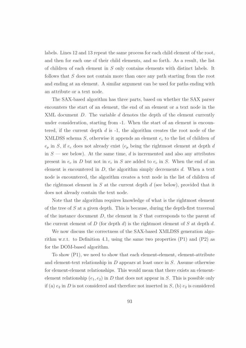
labels. Lines 12 and 13 repeat the same process for each child element of the root,
and then for each one of their child elements, and so forth. As a result, the list
of children of each element in S only contains elements with distinct labels. It
follows that S does not contain more than once any path starting from the root
and ending at an element. A similar argument can be used for paths ending with
an attribute or a text node.
The SAX-based algorithm has three parts, based on whether the SAX parser
encounters the start of an element, the end of an element or a text node in the
XML document D. The variable d denotes the depth of the element currently
under consideration, starting from -1. When the start of an element is encoun-
tered, if the current depth d is -1, the algorithm creates the root node of the
XMLDSS schema S, otherwise it appends an element ec to the list of children of
ep in S, if ec does not already exist (ep being the rightmost element at depth d
in S — see below). At the same time, d is incremented and also any attributes
present in ec in D but not in ec in S are added to ec in S. When the end of an
element is encountered in D, the algorithm simply decrements d. When a text
node is encountered, the algorithm creates a text node in the list of children of
the rightmost element in S at the current depth d (see below), provided that it
does not already contain the text node.
Note that the algorithm requires knowledge of what is the rightmost element
of the tree of S at a given depth. This is because, during the depth-first traversal
of the instance document D, the element in S that corresponds to the parent of
the current element of D (for depth d) is the rightmost element of S at depth d.
We now discuss the correctness of the SAX-based XMLDSS generation algo-
rithm w.r.t. to Definition 4.1, using the same two properties (P1) and (P2) as
for the DOM-based algorithm.
To show (P1), we need to show that each element-element, element-attribute
and element-text relationship in D appears at least once in S. Assume otherwise
for element-element relationships. This would mean that there exists an element-
element relationship (e1, e2) in D that does not appear in S. This is possible only
if (a) e2 in D is not considered and therefore not inserted in S, (b) e2 is considered
93

Panel 2: XMLDSS Extraction Algorithm (SAX-based)
Input: XML document D
Output: XMLDSS schema S in its DOM representationd:=-114
if (encountered the start of an element named elem with attributes atts)15
thenif (d==-1) then16
Create Element r with label elem17
Set r to be the root of XMLDSS schema S.18
else19
Let ep be the rightmost element at depth d in S20
Let children be the list of children of ep in S21
if (children does not contain an element with label elem) then22
Create Element ec with label elem23
Append ec to children in S24
Increase d by 125
Set r or ec to be the rightmost element at depth d in S26
for (each attribute a in atts) do27
if a does not exist in ec then add to ec an Attribute with label a28
else if (encountered the end of an element named elem ) then29
Decrease d by 130
else if (encountered a text node) then31
Let ep be the rightmost Element of S at depth d32
Let children be the list of children of ep in S33
if (children does not contain any text nodes) then34
Append text node with content “Text” to the list of children of ep35
94

but not added to S or (c) e2 is added erroneously to the list of children of another
element e3 in S. The first case cannot occur because of line 15 in Panel 2, which
shows that every element in D is considered. The second case cannot occur
because of lines 17-18 and 23-24, which show that every element in D is added
in S, unless it is already present in the list of children of a certain element. The
third case cannot occur because when the current pointer in D is at an element e,
the current pointer in S is at the corresponding element e in S. This is achieved
by maintaining the rightmost element of S for each individual depth value d:
when the current element in D at depth d is e2 and has parent element e1, the
rightmost element of S at that depth has the same label as e1 in D. A similar
argument can be used for element-text and element-attribute relationships.
To show (P2) we use structural induction, having as a starting point the fact
that D and S have the same root (lines 17-18). As discussed above, an element e
cannot be added to the list of children of an element p in S if it is already present
(lines 22-24), and so the list of children of an element e in S cannot contain
the same element twice. Therefore, the root of S only contains elements with
distinct labels. This process is repeated for each element encountered in D by
means of depth-first traversal using the event-based SAX API. As a result, the
list of children of each element in S only contains elements with distinct labels. It
follows that S does not contain twice any path starting from a root and ending at
an element. A similar argument can be used for paths ending with an attribute
or a text node.
Both algorithms have a complexity of O(E+A+T ), where E, A and T are the
numbers of elements, attributes and text nodes in D respectively. The SAX-based
algorithm has the advantage that, because it is event-based and therefore does
not need to load D into memory first in order to extract its XMLDSS schema, it
avoids a possible memory problem when dealing with large XML documents.
Automatic XMLDSS derivation from a referenced DTD
While it is possible to extract an XMLDSS schema from an XML document
itself, being able to derive it from the DTD or XML Schema accompanying the
95

document could be beneficial for two reasons. First, if the XML document is
large, then deriving the XMLDSS schema from an existing DTD or XML Schema
is likely to be more efficient. Also, deriving an XMLDSS schema from an existing
DTD or XML Schema avoids possible XMLDSS schema evolution problems. This
is because the XMLDSS schema that is extracted from an XML document has
the characteristics of a structural summary, i.e. describes the current structure of
the XML document. An XMLDSS schema derived from a DTD or XML Schema
schema, however, describes not only the current structure of the XML document,
but could also contain structure not currently present in the XML document and
representing possible future evolutions of the document.
Another reason for developing algorithms for the derivation of an XMLDSS
schema from an existing DTD or XML Schema is to be able to support homoge-
neous collections of XML documents in native XML databases (NXDBs). If all
documents in a homogeneous collection in an NXDB conform to the same DTD
or XML Schema, then deriving an XMLDSS from this DTD or XML Schema
enables our approach to handle such a collection as a single data source.
Our algorithm for deriving an XMLDSS schema S for an XML document D
from a given DTD T first scans T and populates two auxiliary data structures:
T1 for storing element names and their content model2, and T2 for storing element
names and the attributes related to them. Since multiple XML documents with
different root nodes can conform to the same DTD, our algorithm first inspects
D to infer the appropriate element declaration ed in T . Using ed, we create the
corresponding element es in S, then retrieve from T2 the attribute declarations
relevant to ed and create the corresponding attributes for es in S. Then, the
content model of ed is retrieved from T1 and processed: for each item i in the
content model, if i is an element, the same process as for ed is applied; if it is a
PCDATA or a CDATA node declaration, the corresponding text node is created
in S.
To illustrate, Table 4.3 shows an example DTD and Figure 4.3 shows the
2The content model for an element e in a DTD defines the elements ei allowed in the listof children e, their ordering within that list and the cardinality of each element ei.
96

XMLDSS schema derived from this DTD.
Since declarations in a DTD can be listed in any order, we scan the whole
of T and populate data structures T1 and T2 first; otherwise multiple scans of T
would have to be performed. We currently do not consider entity and notation
declarations, and this is an area of future work.
<!ELEMENT author (name)><!ATTLIST author id ID #REQUIRED><!ELEMENT author-ref EMPTY><!ATTLIST author-ref id IDREF #REQUIRED><!ELEMENT book (isbn, title, author-ref*)><!ATTLIST book id ID #REQUIRED><!ELEMENT isbn (#PCDATA)><!ELEMENT library (book+,author*)><!ELEMENT name (#PCDATA)><!ELEMENT title (#PCDATA)>
Table 4.3: Example DTD.
XMLDSS DOM
library$1_7
name$1_7
author$1_7
Text
book$1_7
Text
isbn$1_7 title$1_7
Text
author_ref$1_7 id
id id
Figure 4.3: XMLDSS Derived from the DTD of Table 4.3 or from the XMLSchema of Table 4.4.
97

Automatic XMLDSS derivation from a referenced XML Schema
In contrast to DTD where all declarations have global scope, in XML Schema
it is possible to define both global and local declarations. A global declaration
is always named so that it can be referenced, and is a child element of the root
node of the XML Schema, whereas a local declaration is always unnamed and
is a child of the declaration to which it refers, e.g. a local attribute declaration
appears in the list of children of the element it refers to.
XML Schema allows more types of declarations than does DTD. Our algo-
rithm for deriving an XMLDSS schema S for an XML document D using a given
XML Schema T therefore uses five internal data structures, T1, . . . , T5, to respec-
tively store element declarations, attribute declarations, simple and complex type
declarations, model group declarations3 and attribute group declarations4.
We first retrieve the child elements of the root node of T (the global declara-
tions) and store them in T1, . . . , T5. Since multiple XML documents with different
root nodes can conform to the same XML Schema, we then inspect D to infer
the appropriate global element declaration et in T . We then retrieve the type of
et which may be defined using a globally declared simple or complex type, or via
referencing another globally declared element declaration.
Simple type declarations define data types, so if et in T references such a dec-
laration, we create a text node for es in S, if one does not already exist. The
same applies for complex type declarations that have simple content which also
only allows character content. The other option for a complex type is to contain
a complex content declaration. This may contain one or more attribute or at-
tribute group declarations, element declarations or model group declarations. An
attribute declaration is processed by adding the respective attribute to es, while
an attribute group declaration is processed by handling each attribute declara-
tion similarly. Element declarations are processed by appending an element to
the list of children of es, then processing the type of the element. As a result,
3Model groups are similar to complex type declarations, but do not allow inheritance andtherefore cannot be extended or restricted.
4An attribute group contains related attributes that are commonly used together.
98

the XMLDSS schema S is created in a depth-first manner. Finally, model group
declarations in complex types are processed by handling each element declaration
as above.
Our algorithm ignores a number of XML Schema aspects, such as annotations
and key/keyref declarations, as these do not contribute to the content of an
XMLDSS schema. We also currently ignore a number of XML Schema features,
such as substitution groups, and this is an area of future work. Table 4.4 lists an
example XML Schema and Figure 4.3 illustrates the derived XMLDSS schema.
4.3 Overview of our XML Data Transformation/
Integration Approach
We have separated the process of transforming or integrating XML data sources
into two steps. First, a schema conformance phase conforms the source and
target schemas, overcoming the problems stemming from semantic heterogeneity.
Then, a schema transformation phase transforms the source schema into a target
schema, in the case of a data transformation setting, or integrates a set of source
schemas under a global schema, in the case of a data integration setting.
For clarity of presentation, we first present the different application settings
for the schema transformation phase, assuming that there is no semantic het-
erogeneity. We then drop this assumption and show how our approach handles
semantic heterogeneity within the schema conformance phase.
4.3.1 Schema Transformation Phase
The schema transformation phase can be applied in three distinct settings: in
a peer-to-peer data transformation setting, where two peers wish to allow the
exchange of data between them; in a top-down data integration setting, where the
global schema is predefined and the data source schemas need to be transformed
to match it, regardless of any loss of information that may occur; or in a bottom-
up data integration setting, where there is no predefined global schema and the
99

<xs:schema xmlns:xs="http://www.w3.org/2001/XMLSchema"
targetNamespace="http://www.dcs.bbk.ac.uk/~lucas"
xmlns="http://www.dcs.bbk.ac.uk/~lucas" elementFormDefault="qualified">
<xs:attribute name="id" type="xs:string"/>
<xs:element name="library">
<xs:complexType>
<xs:element name="book" type="bookType" minOccurs="1" />
<xs:element name="author" type="authorType" minOccurs="0" />
<xs:key name="bookKey">
<xs:selector xpath="./book"/> <xs:field xpath="@id"/>
</xs:key>
<xs:key name="authorKey">
<xs:selector xpath="./author"/> <xs:field xpath="@id"/>
</xs:key>
<xs:keyref name="bookAuthorKeyRef" refer="bookKey">
<xs:selector xpath="//book/author-ref"/> <xs:field xpath="@id"/>
</xs:keyref>
</xs:complexType>
</xs:element>
<xs:complexType name="bookType">
<xs:all>
<xs:element name="isbn" type="xs:string" minOccurs="1"maxOccurs="1"/>
<xs:element name="title" type="xs:string"minOccurs="1"maxOccurs="1"/>
<xs:element name="author-ref" type="authorKeyRefType" minOccurs="1"/>
<xs:comlexType>
<xs:attribute name="id" use="required"/>
</xs:complexType>
</xs:element>
</xs:all>
<xs:attribute name="id" type="xs:string" use="required"/>
</xs:complexType>
<xs:complexType name="authorType">
<xs:all>
<xs:element name="name" type="xs:string" minOccurs="1"maxOccurs="1">
<xs:comlexType>
<xs:attribute name="id" use="required"/>
</xs:complexType>
</xs:element>
</xs:all>
<xs:attribute name="id" type="xs:string" use="required"/>
</xs:complexType>
</xs:schema>
Table 4.4: Example XML Schema.
100

information from all the data sources needs to be preserved within the global
schema that is generated.
To support these three different settings, we have developed a schema restruc-
turing algorithm (SRA), which automatically restructures a source schema S to
a target schema T , eliminating schematic heterogeneity. The SRA restructures S
into T using the BAV approach, thus creating a transformation pathway S → T
— the inverse pathway S ← T can then be automatically derived due to the
reversibility of BAV transformations. We assume that S and T have been pre-
viously semantically conformed, i.e. that the earlier schema conformance phase
has addressed any 1–1, 1–n, n–1 and n–m semantic relationships between schema
constructs of S and T (see discussion on semantic heterogeneity in Chapter 2).
Therefore, we consider an element in S to be equivalent to an element in T if and
only if they have the same element identifier elementName$count.
We give a high-level description of the SRA below, where we discuss the appli-
cation of the schema transformation phase in the three transformation/integration
settings. The SRA is discussed in detail in Chapter 5, together with an evaluation
of its complexity. Chapter 6 then discusses an extension of the SRA, which is
able to use information that identifies an element/attribute in S to be equivalent
to, a superclass of, or a subclass of an element/attribute in T .
We now consider in turn each one of the three settings that our schema trans-
formation phase supports. We also discuss the correctness of the application of
the SRA in each setting.
Peer-to-peer data transformation
Figure 4.4 illustrates a peer-to-peer transformation setting, where schemas S1 and
S2 of peers P1 and P2 need to be mapped for the purpose of exchanging data be-
tween P1 and P2. In this setting, the schema transformation phase takes as input
schemas S1 and S2 and produces a transformation pathway that contains a grow-
ing phase followed by a shrinking phase. In the growing phase, constructs from
S2 not present in S1 are inserted into S1 and, in the shrinking phase, constructs
from S1 not present in S2 are removed from S1.
101

The schema transformation phase in this setting is supported by our schema
restructuring algorithm (SRA). Since BAV pathways are bidirectional, the shrink-
ing phase in pathway S1 → S2 is a growing phase in the reverse pathway, S1 ← S2.
For this reason, the SRA has been implemented so that it applies a growing phase
both on S1, producing intermediate schema IS1, and on S2, producing interme-
diate schema IS2. These intermediate schemas are identical and this is asserted
by automatically injecting a series of id transformations between them, using the
AutoMed API.
S 1 IS 1 data
source
id data
source IS 2 S 2
Figure 4.4: Peer-to-Peer Transformation Setting.
We note here that if a construct c in S2 is not present in S1, then the SRA adds
c in S1 with an extend transformation and the query Range Void Any, which implies
loss of information. However, as we will discuss in Chapter 5, if c is an Element
construct, the SRA could use an add transformation instead, by generating a
synthetic extent for c, and prevent the loss of information of descendant constructs
of c. The decision of whether or not the SRA should generate a synthetic extent
when possible is made by the user, before the application of the SRA.
After creating a BAV transformation pathway between schemas S1 and S2,
we can now translate data and queries between P1 and P2. For example, the
transformation pathway S1 ↔ S2 can be used to translate an IQL query expressed
on S2 to an IQL query expressed on S1, and the XML wrapper of S1 can be used to
retrieve the necessary data for answering the query. Or, it can be used to translate
an IQL query expressed on S1 to an IQL query on S2, and the XML wrapper
of S2 can be used to retrieve the necessary data for answering the query. Also,
using our materialisation algorithm that we discuss in Section 4.4.2, it is possible
to materialise S2 using the data source of S1, and vice versa. Our materialisation
algorithm follows a query-based approach, which means that retrieving the extent
102

of each schema construct c of S2 is performed by issuing c as a query on S2, and
then reformulating and evaluating this query on S1.
In terms of the correctness of the application of the SRA in this setting, the
key requirement is that S1 is transformed into S2 in such a way that S1 and S2
are behaviourally consistent5: schemas S1 and S2 are behaviourally consistent if
for any query QS1 over an instance IS1 of S1 there exists a transformation of S1
to S2, of IS1 to an instance of S2, IS2, and of QS1 to a query over IS2, QS2, such
that the results of QS2 are contained in the results of QS1.
Given the bidirectional pathway S1 ↔ S2 produced by the SRA, a query QS1
over an instance IS1 of S1 is rewritten to QS2 on S2 using GAV reformulation
and the delete, contract and rename steps in pathway S1 → S2. In order to
compare the results of QS1 and QS2, we need to evaluate QS2 over the (virtual or
materialised) instance IS2 of S2 produced by applying the add, extend and rename
steps in S1 → S2 to IS1, e.g. by using a GAV-based XMLDSS materialisation
algorithm6. This is equivalent to rewriting QS2 to a query Q′
S1 on S1 using GAV
reformulation and the delete, contract and rename steps in the reverse pathway
S2 → S1 and evaluating Q′
S1 on IS1.7 Therefore, in order to show that the SRA
transforms S1 into S2 in such a way that S1 and S2 are behaviourally consistent
we need to show that the results of Q′
S1 are contained in the results of QS1 for any
query QS1 on S1. We note that all the transformations in the pathway S ↔ T
are used in this setting, and that this transformation pathway does not contain
any additional information that could be further exploited by LAV reformulation
techniques.
5This is a generalisation of the concept of behavioural equivalence [AABN82, BR88] to twoschemas that may not, in general, have the same information capacity.
6Our XMLDSS materialisation algorithm, described in Section 4.4.2, cannot be used as-isfor this task. This is because, when materialising XMLDSS constructs, the algorithm does notretain the instance-level identifiers of the source schema Element and Attribute constructs, butinstead renames them to match those of the constructs being materialised. A version of ourXMLDSS materialisation algorithm that retains the source instance-level identifiers is requiredif it is to be used in the context of this correctness investigation.
7The two are equivalent because both GAV-based materialisation and GAV-based reformu-lation of QS2 to Q′
S1use the same primitive transformations and thus generate the same GAV
views.
103

An example illustrating this discussion is given in Chapter 5, where the SRA
is discussed in detail. A detailed discussion of the correctness of the SRA is given
in Appendix B.
Top-down data integration
Figure 4.5 illustrates a top-down integration setting. In this setting, a global
schema GS is given and the schema transformation phase needs to generate a
transformation pathway between each data source schema LSi and GS, without
necessarily preserving the information capacity of the data source schemas.
The schema transformation phase in this setting is supported by the applica-
tion of the SRA for each pair of schemas (LSi, GS). For each such pair, the SRA
generates a pathway that transforms LSi into GS in the same way as in the peer-
to-peer setting. Thus, from the discussion on the correctness of the peer-to-peer
setting in Appendix B, it follows that each such pair of schemas is behaviourally
consistent.
After creating BAV transformation pathways between each pair of schemas
(LSi,GS), we can now use the AutoMed GQP to process an IQL query Q ex-
pressed on GS against all or some of the data sources. The transformation path-
ways LSi ↔ GS can be used to reformulate Q into an IQL query Qref suitable for
evaluation by the data sources, and the XML wrappers of the data sources can be
used to retrieve the necessary data for answering Qref . Also, the materialisation
algorithm we discuss in Section 4.4.2 can be used to materialise GS using all or
some of the data sources.
As discussed in Chapter 3, the integration semantics in AutoMed are user-
defined, with the default being ‘append’ semantics. In our XML data transfor-
mation and integration approach we use the default semantics. Note that if a
different integration logic were required, e.g. one that deals with the elimina-
tion of duplicates at a data level, schema GS could be transformed further, with
additional queries specifying the integration logic being supplied by the user.
104

ILS i ILS 1
LS i LS 1
DS i
DS 1
ILS n
LS n
DS n
... ...
GS
IGS 1 IGS i IGS n
id id id
Figure 4.5: Top-Down Integration Setting.
Bottom-up data integration
Figure 4.6 illustrates a bottom-up integration setting. In this setting a global
schema does not exist, and the schema transformation phase needs to produce a
global schema GS that preserves all the information of the data sources LS1 . . . LSn,
but that does not contain duplicate Element or Attribute constructs, and also pro-
duce the transformation pathways from LS1 . . . LSn to GS.
An initial global schema may be provided by the user, which is used as a
starting point for producing the global schema. This can be either one of the
data source schemas, or a completely different schema. If the user does not
provide an initial global schema, one of the data source schemas is randomly
chosen for this purpose. In the following, we will assume that the initial global
105

GS 1
LS 2 LS n …
GS 2
GS n
...
restructure
restructure
LS 1
grow
grow
Figure 4.6: Bottom-Up Integration Setting.
schema is data source schema LS1.
The schema transformation phase in this setting is supported by a schema
integration algorithm and the SRA. Using LS1 as the initial global schema, GS1,
our schema integration algorithm (see below) is applied to LS2 and GS1, pro-
ducing a new global schema GS2 that preserves the information capacity of both
LS2 and GS1. LS2 is then restructured to match GS2 by applying the SRA to
LS2 as the source schema and GS2 as the target schema. Schemas LS3, . . . , LSn
are integrated similarly: for each LSi, we first apply the schema integration algo-
rithm to LSi and GSi−1, producing the new global schema GSi that preserves the
information capacity of both LSi and GSi−1; we then restructure LSi to match
GSi, by applying the SRA to LSi and GSi.
106

Our schema integration algorithm applied to each pair LSi and GSi−1 pro-
duces a schema GSi that contains all constructs of GSi−1 and all concepts8 of
LSi. The algorithm consists only of a growing phase, which uses extend transfor-
mations to add to GSi−1 those Element and Attribute constructs that are present
in LSi but not in GSi−1.
Note that, if schema GSi−1 already contains ElementRel constructs 〈〈i, p, e〉〉
and 〈〈j, e, Text〉〉, we do not add to GSi−1 an Attribute construct 〈〈p, e〉〉, since
the SRA can derive the extent of 〈〈p, e〉〉 by joining the two latter constructs.
Similarly, we do not add to GSi−1 an Element 〈〈e〉〉 with parent 〈〈p〉〉 if GSi−1
already contains an Attribute 〈〈p, e〉〉, since the SRA can derive the extents of 〈〈e〉〉,
〈〈i, p, e〉〉 and 〈〈j, e, Text〉〉 using the extent of 〈〈p, e〉〉 (thus, there is no information
loss in terms of Element and Attribute constructs, since the application of the
SRA on LSi and GSi results in only add and delete transformations for such
constructs).
Also, we do not add any ElementRel constructs present in LSi but not in
GSi−1, because it is possible to derive their extents through the use of path
queries on GSi−1. When deleting these ElementRel constructs from LSi, the SRA
is able to use delete transformations, rather than contract ones, depending on
whether or not the user has opted for synthetic extent generation (as per our
discussion for the peer-to-peer setting). Similarly, ElementRel constructs present
in GSi but not in LSi are added to LSi using add transformations, if the user
has opted for synthetic extent generation, otherwise extend transformations may
also be used. Thus, when the SRA is applied to LSi and GSi, if the user opts
for synthetic extent generation, only add and delete transformations are used
regarding ElementRel constructs; otherwise, extend and contract transformations
may also be used.
We give more details of this algorithm in Chapter 5. We note that our schema
8Since the SRA is able to perform element-to-attribute and attribute-to-element transfor-mations, adding to GSi−1 Element constructs of LSi that are present in GSi−1 as Attributeconstructs, and vice versa, will not add any information to GSi−1. Therefore, our schema inte-gration algorithm does not add to GSi−1 such constructs of LSi., since the concepts they referto are already present in GSi−1
107

integration approach follows the ladder strategy [BLN86], which was discussed in
Chapter 2.
Regarding the correctness of our bottom-up integration setting, we need to
show that the final global schema GSn preserves the information capacity of all
data sources LS1 . . . LSn. This amounts to showing that, given a pair of schemas
(LSi, GSi−1), the new global schema GSi preserves the information capacity of
both LSi and GSi−1. First, we note that GSi preserves the information capacity
of GSi−1, since it is produced by applying only extend transformations to GSi−1.
Therefore, any query QGSi−1 on GSi−1 will have the same results with query
Q′
GSi−1, produced by reformulating QGSi−1 first using pathway GSi−1 → GSi,
and then using pathway GSi → GSi−1. Second, we need to show that GSi
preserves the information capacity of LSi. As discussed above, if the user opts
for synthetic extent generation, the pathway LSi ↔ GSi does not contain any
extend or contract steps; otherwise, the pathway may also contain extend and
contract steps. Therefore, any pair of queries QLSi and Q′
LSi on LSi, where
Q′
LSi is produced by reformulating QLSi first using pathway LSi → GSi, and
then using pathway GSi → GSi, will have the same results if the user opts for
synthetic extent generation; otherwise the results of Q′
LSi will be contained in the
results of Q′
LSi.
The structure of the final global schema GSn clearly depends on the order
of integration of LS1, . . . , LSn, in that it will be identical to LS1, successively
augmented with missing constructs appearing in LS2, . . . , LSn. If a different
integration order is chosen, then the structure of the final global schema may be
different, although containing the same concepts (see Footnote 8).
After the integration of schemas LS1 . . . LSn and the generation of the global
schema GSn, we can use the AutoMed GQP to process queries expressed on GSn
against all or some of the data sources, and we can also materialise GSn using all
or some of the data sources. Global querying and materialisation are discussed
in Section 4.4.
108

4.3.2 Schema Conformance Phase
The schema conformance phase handles problems originating from semantic and
data type heterogeneity between schemas. Chapter 2 provided a review of such
problems along with a number of techniques used for overcoming them.
Our XML data transformation and integration approach does not constrain
the method used to perform schema conformance. Here we briefly describe two
such methods: using schema matching [RB01] and using correspondences to on-
tologies [ABFS02]. Both methods can be used to generate fragments of AutoMed
transformation pathways semi-automatically. Different schema conformance tech-
niques could have different outputs in terms of the fragments of transformation
pathways generated. For example, in a peer-to-peer setting, it is most natural
for schema matching techniques to modify only one of the two schemas, e.g. S1,
producing a new schema S ′
1 and a pathway S1 ↔ S ′
1. Conversely, a technique
using correspondences to ontologies would most naturally modify both schemas
and produce two new schemas S ′
1 and S ′
2 and transformation pathways S1 ↔ S ′
1
and S2 ↔ S ′
2. We now discuss both approaches in more detail.
Schema conformance using schema matching
A schema matching tool (such as COMA++ [ADMR05]) can be used to au-
tomatically produce matches between two XMLDSS schemas S1 and S2, which
(possibly after manual refinement) can then be used to automatically transform
either schema S1 into an intermediate schema S ′
1 or schema S2 into an interme-
diate schema S ′
2.
As discussed in Chapter 2, the matches between schemas S1 and S2 would
be of four types, 1–1, n–1, 1–n and n–m. In our context, these matches can be
used to generate 1, 1, n or m add transformations, followed by 1, n, 1 or n delete
transformations, respectively. Chapter 5 explores the application of this schema
conformance technique.
109

Schema conformance using ontologies
Consider a setting in which two XMLDSS schemas S1 and S2 are each semantically
linked to an ontology, O, by means of a set of correspondences. Assume that the
language in which O is defined is known to the AutoMed MDR and that O is
expressed as an AutoMed schema. The correspondences may be defined by a
domain expert or extracted by a process of schema matching from the XMLDSS
schemas and/or underlying XML data. Each correspondence maps an XMLDSS
element or attribute construct to an IQL query over the ontology schema, and
there may be more than one correspondences for the same XMLDSS construct
(so the correspondences are potentially GLAV mappings).
Then, these correspondences can be used to automatically generate trans-
formation pathways from S1 and S2 to intermediate schemas S ′
1 and S ′
2. The
schemas S ′
1 and S ′
2 will be conformed, in the sense that they will use the same
terms for the same ontology concepts.
It is also possible to cater for settings where schemas S1 and S2 are linked to
different ontologies O1 and O2, provided that there already exists an AutoMed
transformation pathway between O1 and O2, possibly via one or more interme-
diate ontologies. In such a setting, the initial set of correspondences C1 between
S1 and O1 can be automatically transformed into a new set of correspondences
C ′
1 between S1 and O2, and the original setting where two XMLDSS schemas S1
and S2 are linked to the same ontology will now apply. The application of this
schema conformance technique is discussed in more detail in Chapter 6.
4.4 Querying and Materialisation
After the schema conformance and schema transformation phases have removed
semantic and schematic heterogeneities between the source and the target or
global schemas, the target or global schema can be queried or materialised.
This section discusses XML-specific query processing and materialisation as-
pects of AutoMed. We first describe the XML Wrapper components that we
110

have developed for the AutoMed Wrapper architecture, introduce instance-level
unique identifiers for XML data sources and explain their usage, and present a
component for translating XQuery queries, submitted to an XMLDSS schema,
into IQL queries on the same schema. We then present two algorithms for mate-
rialising an XMLDSS schema, S, using data from one or more of the data sources
that S is linked to via AutoMed transformation pathways. The first algorithm
uses the AutoMed Query Processor to materialise S, and the second algorithm
generates an XQuery query for performing the same task, i.e. does not interact
with AutoMed when executed.
4.4.1 Querying an XMLDSS Schema
AutoMed XML Wrappers
The AutoMed XML Wrapper components and their relationship with the ab-
stract AutoMedWrapper and AutoMedWrapperFactory components are illustrated
in Figure 4.7.
The functionality of the XMLWrapperFactory component is twofold. First, to
define the XMLDSS modelling language in the MDR component of the AutoMed
Metadata Repository, if it does not already exist. Second, it contains a number
of XML-specific options which the XMLWrapper instances it produces take into
consideration. One of these options specifies whether an XML data source will
be validated against its accompanying DTD or XML Schema, if one exists. The
other options are in regard to handling of whitespace, i.e. whether whitespace
will be preserved or not when querying a data source.
The XMLWrapper component implements querying functionality common to
any type of XML Wrapper, such as translating an IQL scheme to an XPath query,
and also defines the functionality that its subclasses must implement. Currently,
the XML data integration toolkit supports DOM-based and SAX-based Wrappers
for XML documents, and also XML documents stored within the eXist9 native
XML database.
9See http://exist.sourceforge.net/
111

SAX Wrapper
NXDB Wrapper
SAX Wrapper Factory
AutoMed Wrapper
AutoMed Wrapper Factory
NXDB Wrapper Factory
eXist data source
XML Wrapper
XML Wrapper Factory
DOM Wrapper
DOM Wrapper Factory
eXist Wrapper
eXist Wrapper Factory
XML File
XML File
Figure 4.7: The AutoMed XML Wrapper Architecture.
The DOMWrapper can accept simple node and edge queries and translates
these into XPath queries. The SAXWrapper supports the same types of queries
and is preferable for large XML documents which could create memory problems
for the DOM-based wrapper. The NXDBWrapper can currently translate only
IQL schemes into XPath expressions, but it is currently being extended to be
able to translate IQL queries representing select-project-join-union queries into
XQuery FLWR expressions. Finally, the EXISTWrapper interacts with an eXist
data source and evaluates the queries produced by the NXDBWrapper.
Instance-Level Unique Identifiers
As discussed in Section 4.2.3, each element in an XMLDSS schema is identified
by an identifier of the form elementName$count sid. While the element name,
the element counter and the schema identifier are sufficient for disambiguating
between elements in XMLDSS schemas, another counter is needed to uniquely
112

identify between instances of an XMLDSS element within AutoMed. We therefore
use instance-level unique identifiers for element instances, which are of the form
elementName$count sid&instanceCount, where instanceCount is the instance
counter. Each XML Wrapper type is responsible for generating this identifier
on-the-fly when retrieving data from an XML data source.
Note that if a schema S has been transformed to a schema T , then the result
of a query submitted on T and evaluated over the data source of S may contain
Element instance-level identifiers that do not correspond to the schema-level iden-
tifier(s) of T specified in the query, due to the transformations in S → T . While
this is to be expected when querying T over the data source of S, Section 4.4.2
discusses how our materialisation algorithm does conform the instance-level iden-
tifiers of S to the schema-level identifiers of T when materialising T using the
data source of S.
XQuery Translation
As discussed in Chapter 3, AutoMed’s Translator component is used to translate
queries expressed in a high-level query language into IQL queries. This component
serves as an abstract class and gives no implementation for any specific query
language.
We have therefore developed the XQueryTranslator component, which can be
used to translate XQuery user queries submitted to an XMLDSS schema into
IQL queries and pass these on to the GQP for further processing and evaluation.
The component is also responsible for translating IQL results back into XQuery
to present to the user.
The XQueryTranslator is able to translate a subset of XQuery into IQL. In par-
ticular, it can translate IQL queries representing select-project-join-union queries
into XQuery FLWR expressions. Figure 4.8 illustrates the end-to-end support for
XQuery in the AutoMed system, assuming interaction with an eXist data source.
As an example, consider the following query submitted for evaluation against
the XML document of Figure 4.1 stored in an eXist database (its corresponding
XMLDSS schema is shown in Figure 4.2):
113

for $x in /root/customer,
$y in $x/name/text(),
$z in $x/account/site/function/text()
where $z = "Business"
return $y
IQL query
GQP XQuery Translator
eXist data source IQL
result
eXist Wrapper
XQuery query
XQuery result
IQL query
IQL result
XQuery query
XQuery result
Figure 4.8: Translation to and from XQuery in AutoMed.
The query is first translated by the XQueryTranslator into the following IQL query:
[$y|{$xroot1, $xcustomer1} ← 〈〈1, root$1, customer$1〉〉;
{$xcustomer1, $zaccount1} ← 〈〈2, customer$1, account$1〉〉;
{$zaccount1, $zsite1} ← 〈〈2, account$1, site$1〉〉;
{$zsite1, $zfunction1} ← 〈〈2, site$1, function$1〉〉;
{$zfunction1, $z} ← 〈〈1, function$1, text〉〉;
{$xcustomer1, $yname1} ← 〈〈1, customer$1, name$1〉〉;
{$yname1, $y} ← 〈〈2, name$1, text〉〉; (=) $z ′Business′]
The EXISTWrapper can currently handle only single-scheme queries, therefore
the GQP sends each of the above to the EXISTWrapper, which translates them to
equivalent XPath queries. The wrapper then submits these XPath queries to the
eXist database, receives the query results and formulates the IQL extents of the
schemes based on these results. The results are then passed back to the GQP,
to proceed with the evaluation of the query. The IQL result obtained from the
GQP is as follows:
[’John Smith’,. . .]
114

and is returned to the XQueryTranslator, which will then translate the IQL result
into a valid XQuery result.
4.4.2 Materialising an XMLDSS Schema Using AutoMed
This section describes the materialisation of an XMLDSS schema S using data
from one or more of the data sources that S is linked to via AutoMed transfor-
mation pathways. Our materialisation algorithm is listed in Panel 3. We see that
it first materialises the root node of S, RS, along with any attributes and text
nodes it may have, and then considers all ElementRel constructs in a depth-first
fashion to materialise all other schema constructs. It obtains the data needed
to populate a schema construct by invoking AutoMed’s Global Query Processor
(GQP) using the schema construct as the global query and employing GAV query
reformulation.
An issue that arises during the materialisation is to ensure the correct parent-
child relationships in S. For this purpose, we exploit the instance-level unique
identifiers of the ElementRel constructs to correctly identify the parent of each
element instance (line 42 of Panel 3).
As discussed in Section 4.4.1, when a query is submitted to S, the result may
contain instance-level Element identifiers that do not correspond to the schema-
level Element identifier of S specified in the query. Our materialisation algorithm
uses the schema-level identifier of S specified in the query together with the
size of the query result to create the correct labels for Element instances in the
materialised instance of S (line 43). This means that if we were to re-extract the
XMLDSS schema from the materialised instance, this would be identical to S.
Our materialisation algorithm assumes that the size of the extent of the root
node is exactly 1. However, it is possible that in an integration scenario, a target
or global schema may have a root element whose extent size is greater than 1.
Such cases can be handled in three different ways, according to the needs of the
integration setting.
The first solution is to introduce a generic root node Rgeneric in the materialised
115

Panel 3: XML DataSource Schema Materialisation Algorithm
Input: XMLDSS schema S in its DOM representation; data sourceschemas LSi and their associated data sources DSi; AutoMedrepository containing the transformation pathways LSi → S
Output: Doc — XML document which is an instance of S, both as DOMdocument in memory and as file on disk
// Create the root node of DOM document
Create the root element, RDoc, of Doc, setting its name to be the name of36
the root element of S, RS.Create the attributes of RDoc, setting their name to be the same as the37
attributes of RS (if any); populate the attributes by retrieving theirextents using the GQP.// Create the rest of the DOM document:
for (every non-root element CS in S in a depth-first traversal of S) do38
Let PS be the parent of CS in S and PDoc be the (already materialised)39
instances of PS in Doc.Retrieve the extent of 〈〈P, C〉〉 using the GQP.40
for (every pair (p, c) in the extent of 〈〈P, C〉〉) do41
Locate element p in PDoc.42
Append c to the list of children of p.43
Materialise the attributes of c in the same manner as the attributes44
of RDoc in step 37.
Serialise the DOM document to a file on disk.45
instance. The list of children of Rgeneric will contain the instances of the actual
root node of S. This solution violates the definition of XMLDSS in that Rgeneric
is not present in S, but this may not be problematic in the given setting.
The second solution resolves the problem by introducing a generic root node
Rgeneric into S prior to materialisation, thus forming a new schema S ′, then
materialising S ′ instead of S. This solution involves creating a synthetic extent
for Rgeneric and for the ElementRel from Rgeneric to the actual root node of S.
The third solution considers the fact that homogeneous collections in native
XML databases are designed to contain a number of documents with the same or
similar structure. In such a setting, the materialisation algorithm can materialise
S by producing n XML documents, where n is the size of the extent of the root
116

node of S.
Our materialisation algorithm is tree-based: the instance of S is first created
in memory using DOM, then serialised in an XML document on disk using an
existing DOM-based serialisation engine. This means that the algorithm can
be significantly affected in terms of performance when materialising large XML
documents, due to large memory consumption.
The solution to this problem would be to provide an event-based material-
isation algorithm to avoid memory issues. There are many different strategies
that one can follow to develop such an algorithm. One strategy is to traverse
the XMLDSS schema in a depth-first or breadth-first fashion and materialise one
construct at a time, maintaining at the same time multiple pointers in the mate-
rialised document. These pointers are needed to be able to determine where to
insert the instances of the current construct without reparsing the materialised
document — this clearly has a greater impact on the breadth-first strategy.
Regardless of the type of the traversal, such an approach would have to update
the document pointers after materialising the instances of a construct. To avoid
the usage of pointers, another strategy would be to materialise the XMLDSS
schema in a document depth-first fashion, i.e. first materialise the root of the
document, then the first child instance of the root, then the first child instance
of that element etc. This strategy does not require document pointers, but has
two disadvantages. First, we would need to keep a record of which instances of
each construct have been materialised, and, second, we would need to query each
construct as many times as the number of instances of its extent — except, of
course, if it has no child instances.
It is evident from this discussion that developing an event-based materiali-
sation algorithm is not straightforward and we leave this as a matter of future
work.
117

4.4.3 Materialising an XMLDSS Schema Using XQuery
The previous section presented an algorithm that uses the AutoMed’s GQP to
materialise an XMLDSS schema S using data from one or more data sources
that S is linked to via AutoMed transformation pathways. We now describe an
algorithm that generates an XQuery query for performing the same task, so that
the materialisation of S does not interact with AutoMed when executed. This
XQuery approach is expected to ease the adoption of our approach by third-party
software tools, assuming they support XQuery. We note that the implementation
of the XQuery generation algorithm is an item of future work.
Our XQuery generation algorithm is listed in Panel 4. We first create the IQL
view v of each construct c of S using AutoMed’s GQP and GAV reformulation
(line 48), and then translate each v into an equivalent XQuery query vx (line 49).
Our IQL-to-XQuery translator currently supports a subset of the XQuery query
language, and in particular can translate select-project-join-union IQL queries
into XQuery FLWR expressions. We also note that the schema restructuring al-
gorithm described in Chapter 5 and the extended schema restructuring algorithm
described in Chapter 6 use custom IQL functions to generate synthetic extent and
avoid loss of information during data transformation. Therefore, part of the IQL-
to-XQuery translator’s functionality is to create the equivalent XQuery functions.
We then create a single XQuery query Q for materialising S by following
a bottom-up approach. In particular, we first create the XQuery queries for
materialising the leaf elements ei of S, together with their attributes and child text
nodes (line 53). We then use these queries to create the queries that materialise
the parent elements of ei, together with their attributes and text nodes (line 58-
62). We repeat this process for the parent elements of the parent elements of ei,
and so forth, until query Q is formulated (line 56-63).
In lines 53 and 60, the algorithm creates XQuery queries that are able to mate-
rialise Element constructs of S using data from the data sources of S1 . . . Sn. These
queries create Element instances whose labels are instance-level unique identifiers.
This is because, in order to preserve the correct parent-child relationships in the
materialised instance of S, the XQuery queries in line 60 perform equijoins, and
118
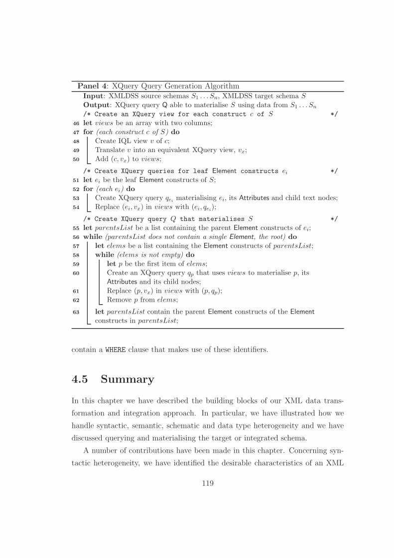
Panel 4: XQuery Query Generation AlgorithmInput: XMLDSS source schemas S1 . . . Sn, XMLDSS target schema SOutput: XQuery query Q able to materialise S using data from S1 . . . Sn
/* Create an XQuery view for each construct c of S */
let views be an array with two columns;46
for (each construct c of S) do47
Create IQL view v of c;48
Translate v into an equivalent XQuery view, vx;49
Add (c, vx) to views;50
/* Create XQuery queries for leaf Element constructs ei */
let ei be the leaf Element constructs of S;51
for (each ei) do52
Create XQuery query qeimaterialising ei, its Attributes and child text nodes;53
Replace (ei, vx) in views with (ei, qei);54
/* Create XQuery query Q that materialises S */
let parentsList be a list containing the parent Element constructs of ei;55
while (parentsList does not contain a single Element, the root) do56
let elems be a list containing the Element constructs of parentsList;57
while (elems is not empty) do58
let p be the first item of elems;59
Create an XQuery query qp that uses views to materialise p, its60
Attributes and its child nodes;Replace (p, vx) in views with (p, qp);61
Remove p from elems;62
let parentsList contain the parent Element constructs of the Element63
constructs in parentsList;
contain a WHERE clause that makes use of these identifiers.
4.5 Summary
In this chapter we have described the building blocks of our XML data trans-
formation and integration approach. In particular, we have illustrated how we
handle syntactic, semantic, schematic and data type heterogeneity and we have
discussed querying and materialising the target or integrated schema.
A number of contributions have been made in this chapter. Concerning syn-
tactic heterogeneity, we have identified the desirable characteristics of an XML
119

schema type in a data integration setting and we have reviewed the most promi-
nent XML schema types against these characteristics. We then introduced a new
XML schema type, XML DataSource Schema (XMLDSS), as a more appropriate
XML schema type for a data transformation/integration setting. This XMLDSS
schema type is used in our approach and supports any regular XML language.
Apart from [YLL03] and Clio [PVM+02], which were developed in parallel with
our work, all other approaches are DTD- or XML Schema-specific.
Concerning application settings, we have defined a modular approach to XML
data transformation and integration which is able to resolve syntactic, schematic
semantic and data type heterogeneity in three distinct settings, namely peer-to-
peer data transformation, top-down data integration and bottom-up data inte-
gration, using a schema conformance and a schema transformation phase. Based
on our discussion of model management in Chapter 2, each of these two phases
could be considered as a model management operator, overloaded to cater for
each of the three settings. Also, each operator would need to provide a different
implementation depending on the approach used, e.g. schema matching or the
use of ontologies for the schema conformance phase. Compared to existing ap-
proaches, our approach distinguishes between schema conformance and schema
transformation as a means of separating the manual and semi-automatic aspects
from the automatic aspects of XML schema and data transformation/integration.
Furthermore, compared to other approaches, we have identified data type hetero-
geneity as a significant issue that needs to be addressed, and Chapter 6 and the
bioinformatics service reconciliation application setting of Chapter 7 discuss this
further.
Concerning querying support, we have developed components for accessing
XML data sources either using XQuery or via the DOM and SAX APIs and we
have also developed a component for translating XQuery into IQL. As a result,
the specifics of IQL query processing in AutoMed are transparent to users of our
XML data transformation and integration toolkit.
In addition to virtual transformation and integration, our approach also caters
for materialised data transformation and integration, as we have also developed
120

two algorithms for materialising an XMLDSS target or global schema. Compared
to the work of [AL05] on materialising a target schema T in an XML data ex-
change setting (discussed in Chapter 2), our approach is focussed on producing
a single instance of T , based on inferring a single BAV pathway between S and
T from the naming and structural relationships between constructs of S and T
(details of this will be presented in Chapter 5, when we describe our SRA al-
gorithm in full). In contrast, the solutions to the XML data exchange problem
studied in [AL05] may be many, and possibly infinite. Our approach produces
a BAV pathway between S and T , and in particular produces GAV mappings
defining the extent of each schema construct of T in terms of those of S. Either
of our materialisation algorithms then use GAV query processing to produce a
single instance of T . In contrast, [AL05] considers the case of an arbitrary set of
given source-to-target dependencies between S and T (which can be thought of
as GLAV mappings), which may or may not be sufficiently informative to infer
a single extent for each schema construct of T . Also, [AL05] generates distin-
guished null values for elements and attributes of T for which data values cannot
be inferred, whereas our approach does not generate any null values.
121

Chapter 5
Schema and Data Transformation
and Integration
5.1 Introduction
In Chapter 4 we introduced our approach to XML data transformation and inte-
gration, and in particular we discussed how our approach handles different XML
data transformation and integration settings. This chapter describes in more de-
tail the schema conformance and schema transformation phases of our approach.
We first investigate a peer-to-peer data transformation setting. We then discuss
the integration of multiple XML data sources in a top-down and in a bottom-up
integration setting.
The chapter is structured as follows. Section 5.2 first presents a running
example for the chapter. Section 5.3 describes how schema matching can be used
as a schema conformance method in our approach. Section 5.4 gives a detailed
description of our schema restructuring algorithm, demonstrates its application
using the running example, and analyses its complexity. Section 5.5 discusses the
integration of multiple XML data sources under a global schema in a top-down or
bottom-up integration setting. Finally, Section 5.6 summarises the contributions
of this chapter.
122

5.2 Running Example for this Chapter
Tables 5.1 and 5.2 illustrate two XML documents, D1 and D2 respectively, con-
taining data about books and their authors. Figure 5.1 illustrates the XMLDSS
schemas of these documents: schema S corresponds to document D1 and schema
T to document D2; schema Sconf relates to the schema conformance phase and will
be discussed in Section 5.3. We note that, for presentational purposes, throughout
this chapter Element constructs will be represented using only their name rather
than their complete schema-level identifiers (which we discussed in Chapter 4).
A first examination of schemas S and T shows that they are quite similar.
One difference is that schema S contains information about publishers, whereas
schema T does not. Further examination also reveals a number of semantic and
schematic differences between them. An example of semantic heterogeneity is
that element 〈〈topic〉〉 in schema S is termed 〈〈genre〉〉 in schema T . An example
of schematic heterogeneity is that while element 〈〈topic〉〉 in S is located under
element 〈〈root〉〉, the equivalent element 〈〈genre〉〉 is located under element 〈〈book〉〉
in T . Another example of schematic heterogeneity is that ISBN information
in S is contained within an element under element 〈〈book〉〉, whereas in T this
information is contained within an attribute attached to element 〈〈book〉〉.
The above examples of heterogeneity can be easily categorised as ‘semantic’
or ‘schematic’. However, it is not always straightforward to determine whether
a matching constitutes a semantic or a schematic heterogeneity problem, and
consequently whether it should be handled by the schema conformance or the
schema transformation phase. Our running example contains two examples of
such matchings. Attribute 〈〈author, dob〉〉 matches attributes 〈〈author, birthday〉〉,
〈〈author, birthmonth〉〉 and 〈〈author, birthyear〉〉 in T (so this is a 1–n matching), and
attributes 〈〈author, firstn〉〉 and 〈〈author, lastn〉〉 in S match element 〈〈name〉〉 and
its link to construct 〈〈Text〉〉 in T (so this is an n–m matching).
Resolving such matchings undoubtedly requires schema transformation. There-
fore, it can be argued that such matchings should be resolved within the schema
123

<root>
<topic type="Sports and Hobbies">
<author firstn="P." lastn="Dawson" dob="1932 01 05">
<book>
<ISBN>J234532677</ISBN>
<title>Principles of Knot-Tying</title>
<publisher>Coles Publishers</publisher>
</book>
<book>
<ISBN>R654354414</ISBN>
<title>Paul Dawson’s Knot Craft</title>
<publisher>Kindersley Ltd</publisher>
</book>
...
</author>
...
</topic>
<topic type="Mathematics">
<author firstn="B.J." lastn="Whitehead" dob="1945 05 07">
<book>
<ISBN>A0B1C1D6E2</ISBN>
<title>Linear Algebra</title>
<publisher>Kindersley Ltd</publisher>
</book>
...
</author>
...
</topic>
...
</root>
Table 5.1: Source XML Document D1
transformation phase by providing the necessary information to that phase. How-
ever, any matching that is not 1–1 essentially addresses a difference in the gran-
ularity of information representation, and, as discussed in Chapter 2, this is a
semantic heterogeneity issue.
Our approach handles such matchings either in the schema conformance phase
or in the schema transformation phase, depending on the schema conformance
technique employed. In this chapter, we assume that schema matching is em-
ployed as the schema conformance technique. This technique is performed pair-
wise between schemas and is able to resolve 1–1, 1–n, n–1 and n–m semantic
124

<root>
<author birthday="05" birthmonth="10" birthyear="1955">
<name>N.A. Buddy</name>
<item>
<book ISBN="0A7B21C6D2">
<title>Principles of Computing </title>
<year>1995</year>
<genre type="Computer Science"/>
</book>
</item>
...
</author>
<author birthday="24" birthmonth="11" birthyear="1951">
<name>K. Ashley</name>
<item>
<book ISBN="K568732253">
<title>Ultimate Book of Knots</title>
<year>2000</year>
<genre type="Sports and Hobbies"/>
</book>
</item>
...
</author>
...
</root>
Table 5.2: Source XML Document D2
heterogeneity. Thus, in this context, the schema restructuring phase just needs
to address 1–1 structural heterogeneity. Chapter 6 explores an alternative ap-
proach to schema conformance, namely using correspondences from each schema
to one or more ontologies. This technique is able to address all types of hetero-
geneity as well, but is performed pairwise between each schema and an ontology,
rather than between the two schemas directly. Thus, S and T are not conformed
with respect to each other, but with respect to one or more ontologies, and so
the schema restructuring phase will need to address other types of heterogeneity
as well, apart from 1–1 structural heterogeneity.
We note that a construct that does not produce a match during the schema
conformance phase is left as it is within a schema, to be handled later by the
schema transformation phase.
125

S conf
book
root
title
1
1
author
Text
1
genre
2
type
publisher
1
3
S
book
root
title
1
1
1
author
Text
1
topic
2
type
ISBN
1
1
firstn
publisher
1
3
dob lastn
T
author
Text
name
1
1
birthday
birthmonth
birthyear birthday
birthmonth
birthyear
name
1
1 1
root
1
book
genre
3
title
1
1
ISBN
type year
2
1
1
item
2
1
ISBN
1
Figure 5.1: Example Source and Target XMLDSS Schemas S and T , and Inter-mediate Schema Sconf , Produced by the Schema Conformance Phase.
5.3 Schema Conformance Via Schema Matching
This section discusses the use of schema matching as the method to detect and
resolve semantic heterogeneity conflicts between two schemas, S and T , in order
to perform schema conformance in our approach. As discussed in Chapter 2,
schema matching may use schema-level and/or data-level information in order
to detect semantic differences between S and T and suggest possible matchings
between them. Regardless of the technique adopted, a schema matching tool
operating on schemas S and T generates a set of 1–1, 1–n, n–1 and n–m matchings
between S and T that may or may not be correct. The user confirms or rejects the
matchings generated. For each of the confirmed matchings, the user also provides
the queries that specify the specific relationship between the schema constructs
of S and T , i.e. mappings between constructs of S and T . These mappings
are then processed by a BAV pathway generation tool that we have developed,
PathGen, which generates a BAV transformation pathway S ↔ Sconf , such that
Sconf is schema S conformed with respect to T . Referring to our running example,
schema S, illustrated on the left of Figure 5.1, is transformed into schema Sconf ,
illustrated in the middle of Figure 5.1.
126

We now describe how PathGen handles each type of matching (1–1, 1–n, n–1,
n–m), and illustrate this using our running example where possible. We note
that a conversion tool is in general required to convert from the output format of
the particular schema matching tool being used to the XML format accepted as
input by PathGen (Appendix A provides the instance of this format as related to
our running example).
When processing a 1–n matching, PathGen generates n add transformations,
each supplied with a user-specified query defining the extent of the new construct
in terms of the original construct, followed by a delete transformation to remove
the original construct (which is now redundant in the schema). In our running
example, suppose that the schema matching tool produces such a match, stating
that dob in S is related to Attribute constructs birthyear, birthmonth and birthday
in T , and that the user then specifies the exact relationship between these at-
tributes using the appropriate IQL queries. This mapping is used by PathGen to
generate the following sequence of transformations on S:
1 addAtt(〈〈author, birthday〉〉,[{x,substring y 8 10}|{x,y}←〈〈author, dob〉〉])
2 addAtt(〈〈author, birthmonth〉〉,[{x,substring y 5 7}|{x,y}←〈〈author, dob〉〉])
3 addAtt(〈〈author, birthyear〉〉,[{x,substring y 0 4}|{x,y}←〈〈author, dob〉〉])
4 deleteAtt(〈〈author, dob〉〉,[{x,concat [y3,’ ’,y2,’ ’,y1]}|{x,y1}←〈〈author, birthday〉〉;
{x,y2}←〈〈author, birthmonth〉〉;
{x,y3}←〈〈author, birthyear〉〉]
In the IQL queries within the transformations above, function concat is used
to concatenate the strings in its input list, while function substring s i1 i2 returns
the substring of s beginning from position i1 and ending at position i2 (inclusive
and non-inclusive respectively).
PathGen processes a 1–1 matching as a special case of a 1–n matching, and
therefore generates one add and one delete transformation in this case. If the
source schema construct has dependent constructs, these need to be handled also.
In our example, suppose that the schema matching tool produces a match stating
that element 〈〈topic〉〉 in S is related to element 〈〈genre〉〉 in T , and that the user
127

specifies that they are equivalent. This information is used by PathGen to add El-
ement 〈〈genre〉〉 (transformation 5 below), associate the dependent constructs of
〈〈topic〉〉 with 〈〈genre〉〉 (transformations 6 - 8 ), then delete the dependent con-
structs of 〈〈topic〉〉 (transformations 9 - 11 ), and finally delete Element 〈〈topic〉〉
(transformation 12 ):
5 addEl(〈〈genre〉〉,〈〈topic〉〉)
6 addAtt(〈〈genre, type〉〉,〈〈topic, type〉〉)
7 addER(〈〈1, root, genre〉〉,〈〈1, root, topic〉〉)
8 addER(〈〈1, genre, author〉〉,〈〈1, topic, author〉〉)
9 deleteAtt(〈〈topic, type〉〉,〈〈genre, type〉〉)
10 deleteER(〈〈1, root, topic〉〉,〈〈1, root, genre〉〉)
11 deleteER(〈〈1, topic, author〉〉,〈〈1, genre, author〉〉)
12 deleteEl(〈〈topic〉〉,〈〈genre〉〉)
Another case of a 1–1 matching in our running example is between ElementRel
〈〈1, author, book〉〉 in S and ElementRel 〈〈2, author, book〉〉 in T . This results in the
following transformations on S:
13 addER(〈〈2, author, book〉〉,〈〈1, author, book〉〉)
14 deleteER(〈〈1, author, book〉〉,〈〈2, author, book〉〉)
When handling an n–1 matching, PathGen generates a single add transfor-
mation, which includes a user-specified query stating how the extents of the n
constructs are combined to create the extent of the new construct. This is fol-
lowed by n delete transformations to remove the n original (and now redundant)
constructs.
Finally, n–m matchings are a generalisation of n–1 and 1–n matchings in that
for these PathGen generates m add transformations to insert the necessary new
constructs, followed by n delete transformations to remove the original constructs.
In our example, the schema matching tool may produce an n–m matching stating
that attributes 〈〈author, firstn〉〉 and 〈〈author, lastn〉〉 in S relate to element 〈〈name〉〉
and its link to 〈〈Text〉〉 in T . After the user provides the appropriate IQL queries,
128

PathGen generates a sequence of add and delete transformations that resolve the
n–m semantic heterogeneity:
15 addEl(〈〈name〉〉, [x|x←generateElement ‘name’ 〈〈author〉〉])
16 addER(〈〈1, author, name〉〉,[{x, y}|{x, y} ← generateElementRel 〈〈author〉〉 〈〈name〉〉]
17 addER(〈〈1, name,Text〉〉,
let q equal [{x,concat [z1,‘ ’,z2]}|{x,z1}←〈〈author, firstn〉〉;{x,z2}←〈〈author, lastn〉〉]
in [{y, z}|{x, y} ← 〈〈1, author, name〉〉; {x, z} ← q])
18 deleteAtt(〈〈author, firstn〉〉,
[{x,substring z 0 (indexOf z ‘ ’)}|{x,y}←〈〈1, author, name〉〉;{y,z}←〈〈1, name,Text〉〉])
19 deleteAtt(〈〈author, lastn〉〉,
[{x,substring z ((indexOf z ‘ ’)+1) ((length z)-1)}|{x,y}←〈〈1, author, name〉〉;
{y,z}←〈〈1, name,Text〉〉])
Transformations 15 – 17 above add Element 〈〈name〉〉, ElementRel 〈〈1, author, name〉〉
and ElementRel 〈〈1, name, Text〉〉, while transformations 18 and 19 remove at-
tributes 〈〈author, firstn〉〉 and 〈〈author, lastn〉〉 from S. The queries in these trans-
formations use IQL function length, which returns the number of characters of
its string argument, IQL function indexOf s1 s2, which returns the position of the
first occurrence of s2 within s1, and IQL function lastIndexOf, which is similar to
indexOf but returns the position of the last occurrence instead of the first. They
also use two XMLDSS-specific IQL functions, generateElement and generateEle-
mentRel. Function generateElement ‘e1’ 〈〈e2〉〉 generates (count 〈〈e2〉〉) instances
for the Element construct whose schema-level identifier is e1. Function genera-
teElementRel 〈〈a〉〉 〈〈b〉〉 produces a list of instances for an ElementRel construct
〈〈k, a, b〉〉, and the size of the extent produced is equal to that of 〈〈b〉〉. This func-
tion assumes that the size of the extent of 〈〈a〉〉 is either equal to that of 〈〈b〉〉, in
which case the ith instance of 〈〈a〉〉 will be associated with the ith instance of 〈〈b〉〉,
or equal to 1, in which case the single instance of 〈〈a〉〉 will be associated with
all instances of 〈〈b〉〉 (this caters for the case when 〈〈a〉〉 is the root node). In any
other case, the input to the generateElementRel function is considered invalid, as
the function would not able to unambiguously associate instances of 〈〈a〉〉 with
instances of 〈〈b〉〉.
129

5.4 Schema Restructuring Algorithm
Section 5.3 has discussed the use of schema matching as the schema conformance
method in our approach and has illustrated the use of this method to conform
schemas S and T of our running example. The schema output by this process,
Sconf in Figure 5.1, together with the target schema, T , are now ready to be
processed by our schema restructuring algorithm (SRA), which implements the
schema transformation phase.
Given Sconf as the source schema and T as the target schema, the SRA trans-
forms Sconf into T . It does so by adding to Sconf all constructs present in T
but not in Sconf (“growing phase”), and then deletes from Sconf all constructs
present in Sconf but not in T (“shrinking phase”). To achieve this, the SRA ap-
plies a growing phase on both Sconf and T , producing new schemas Sres and Tres,
respectively (we recall that, due to the reversibility of AutoMed primitive trans-
formations, the growing phase on T , producing pathway T → Tres, is a “shrinking
phase” in the opposite direction, Tres → T ). Sres and Tres are identical, and this
is asserted by automatically injecting a series of id transformations between them.
Panel 5 presents the SRA. We discuss its three phases, Initialisation, Phase
I and Phase II, in Sections 5.4.1, 5.4.2 and 5.4.3, respectively. As discussed in
Chapter 4, the SRA is able to generate synthetic instances for Element and Ele-
mentRel constructs in order to avoid further loss of information from descendant
constructs. As shown in Panel 5, the user is given the option to permit or not
the generation of such synthetic extent. We discuss this further in the rest of this
section.
Figure 5.2 summarises the schemas and pathways produced by the schema
conformance and the schema transformation phases. Note that, in general, the
schema conformance phase produces two schemas, Sconf and Tconf , as discussed in
Chapter 4. However, schema matching transforms only one of the two schemas, in
this case S, and leaves T unchanged, resulting in the simpler scenario illustrated
in Figure 5.2.
We note that the SRA does not support elements with multiple text nodes,
130
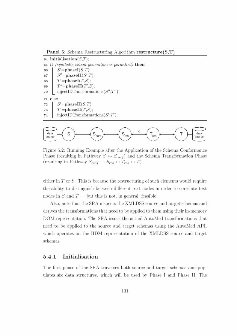
Panel 5: Schema Restructuring Algorithm restructure(S,T)
initialisation(S,T );64
if (synthetic extent generation is permitted) then65
S′=phaseI(S,T );66
S′′=phaseII(S′,T );67
T ′=phaseI(T ,S);68
T ′′=phaseII(T ′,S);69
injectIDTransformations(S′′,T ′′);70
else71
S′=phaseII(S,T );72
T ′=phaseII(T ,S);73
injectIDTransformations(S′,T ′);74
S S conf data
source
id S res T res T data
source
Figure 5.2: Running Example after the Application of the Schema ConformancePhase (resulting in Pathway S ↔ Sconf) and the Schema Transformation Phase(resulting in Pathway Sconf ↔ Sres ↔ Tres ↔ T ).
either in T or S. This is because the restructuring of such elements would require
the ability to distinguish between different text nodes in order to correlate text
nodes in S and T — but this is not, in general, feasible.
Also, note that the SRA inspects the XMLDSS source and target schemas and
derives the transformations that need to be applied to them using their in-memory
DOM representation. The SRA issues the actual AutoMed transformations that
need to be applied to the source and target schemas using the AutoMed API,
which operates on the HDM representation of the XMLDSS source and target
schemas.
5.4.1 Initialisation
The first phase of the SRA traverses both source and target schemas and pop-
ulates six data structures, which will be used by Phase I and Phase II. The
131

Initialisation Phase is not strictly necessary, but it improves the performance of
the SRA since it relieves Phase I and Phase II from two operations that occur
multiple times during the two phases: traversing a schema to identify a certain
construct, and traversing a schema to locate the path between two constructs.
The six data structures created during initialisation are described below:
SourceEl: For every source schema Element, this contains its schema-level iden-
tifier and a pointer to the corresponding DOM element.
TargetEl: For every target schema Element, this contains its schema-level iden-
tifier and a pointer to the corresponding DOM element.
SourceAtt: For every source schema Attribute, this contains its schema-level iden-
tifier and a pointer to the corresponding DOM attribute.
TargetAtt: For every target schema Attribute, this contains its schema-level iden-
tifier and a pointer to the corresponding DOM attribute.
SourceElementRel: For every source schema ElementRel 〈〈ep, ec〉〉1, this contains
the ElementRel identifier, the path between 〈〈ep〉〉 and 〈〈ec〉〉 in the target
schema’s DOM representation, and the type of this path, i.e. whether 〈〈ep〉〉
is an ancestor of 〈〈ec〉〉, or a descendant of 〈〈ec〉〉, or whether 〈〈ep〉〉 and 〈〈ec〉〉
are located in different branches.
TargetElementRel: For every target schema ElementRel 〈〈ep, ec〉〉, this contains
the ElementRel identifier, the path between 〈〈ep〉〉 and 〈〈ec〉〉 in the source
schema’s DOM representation, and the type of this path, i.e. whether 〈〈ep〉〉
is an ancestor of 〈〈ec〉〉, or a descendant of 〈〈ec〉〉, or whether 〈〈ep〉〉 and 〈〈ec〉〉
are located in different branches.
The Initialisation Phase first performs a depth-first traversal of the DOM
representation of the source schema S, during which SourceEl and SourceAtt
1In this chapter, for ease of reading, we omit the first component of an ElementRel 〈〈i, ep, ec〉〉and identify it by just the pair 〈〈ep, ec〉〉, unless the ordering i is significant to the functionalityunder discussion.
132
are populated. TargetEl and TargetAtt are populated similarly using the target
schema T . Then, S is traversed one more time, populating SourceElementRel.
Paths within T are identified with the help of TargetEl: the elements of T with
the same identifiers as 〈〈ep〉〉 and 〈〈ec〉〉 are retrieved, and then successive calls
to retrieve their parent elements are issued, until a common ancestor is found.
TargetElementRel is populated similarly, by traversing T one more time and
using SourceEl.
5.4.2 Phase I - Handling Missing Elements
After the Initialisation Phase, and assuming that synthetic extent generation is
permitted, Phase I is first applied to the source schema and then to the target
schema (Phase I is described in Panel 6, while Panel 7 provides details of the
procedures and functions invoked in Panel 6). For clarity of presentation, we use
the terms ‘source’ and ‘target’ throughout this section assuming that Phase I is
being applied to the source schema. When Phase I is applied to the target schema,
the terms ‘source’ and ‘target’ should be swapped. This includes references made
to the six data structures of Section 5.4.1.
Phase I deals with non-leaf Element constructs present in the target schema
but not in the source schema, i.e. target schema elements that, according to the
schema conformance phase, do not semantically correspond to any source schema
elements or attributes. Phase I adds such target schema Element constructs
(and their associated incoming and outgoing ElementRel constructs) to the source
schema, generating for each of them a synthetic extent. In particular, Phase I
considers each ElementRel 〈〈ep, ec〉〉 of the source schema in a depth-first order,
identifies its corresponding path in the target schema using SourceElementRel
(if such a path exists) and adds to the source schema all the internal Element and
ElementRel constructs of the target schema path.
There are four cases to consider for every ElementRel 〈〈ep, ec〉〉 in the source
schema S and its corresponding path p in the target schema T : 〈〈ep〉〉 may be
the parent of 〈〈ec〉〉 in T , 〈〈ep〉〉 may be an ancestor of 〈〈ec〉〉 in T , 〈〈ep〉〉 may be a
133

descendant of 〈〈ec〉〉 in T , or 〈〈ep〉〉 and 〈〈ec〉〉 may be located in different branches
in T . Figure 5.3 illustrates an example of each of these four cases.
Note that, given an ElementRel 〈〈ep, ec〉〉 corresponding to a target schema path
p, Phase I will create p in the source schema only if all of the internal Element
constructs of p are missing from the source schema. For example, for source
schema ElementRel 〈〈ep, ec〉〉, corresponding to target schema path [ep, K, L, M, ec]
(see top right of Figure 5.3), Element constructs 〈〈K〉〉, 〈〈L〉〉 and 〈〈M〉〉 must not
exist in the source schema. Otherwise, e.g. if 〈〈L〉〉 exists in the source schema but
〈〈K〉〉 and 〈〈M〉〉 do not, then there is ambiguity about the relationships between
〈〈ep〉〉 and 〈〈L〉〉 and between 〈〈L〉〉 and 〈〈ec〉〉, that should have been handled during
the schema conformance phase. In such a case, Phase I leaves it to Phase II to
add to the source schema the missing Element and ElementRel constructs of p
with an undetermined extent, using the query Range Void Any.
The mechanism for our handling of paths whose internal nodes are all missing
from the source schema is skolemisation, i.e. the use of a Skolem function to
generate missing structure between elements that already exist in the source
schema (which are the arguments of the Skolem function). The intention is to
generate such structure automatically in order to avoid loss of information from
the source.
The algorithm of Phase I requires as input the cardinality types of the source
and target schema ElementRel constructs. These are specified in an XML file that
is loaded during Phase I. The cardinality types can either be manually defined by
the user, or can be automatically derived from an accompanying DTD or XML
Schema, or can be automatically derived from sample instances of the source and
target schemas. For example, referring to the example above, the cardinalities of
〈〈A, K〉〉, 〈〈K, L〉〉, 〈〈L, M〉〉 and 〈〈M, B〉〉 may be inferred to be either 1–1 or 1–n.
We note that if the source schema ElementRel has a 1–n cardinality, and the
target schema path does not contain an ElementRel with a 1–n cardinality, then
the setting is inconsistent, and Phase I leaves it to Phase II to add to the source
schema the constructs of the target schema path with an undetermined extent,
using the query Range Void Any. This condition, together with the condition that
134

all internal Element constructs of the target schema path must be missing from
the source schema, is shown in lines 91-94 in Panel 7.
We also note that, if the source schema ElementRel has a 1–n cardinality and
the target schema path contains more than one ElementRel with a 1–n cardinality,
then we assume that just the first such ElementRel construct in the target schema
path has a 1–n cardinality, and that the rest have a 1–1 cardinality (line 98 in
Panel 7). This is further discussed at the end of this section, where we discuss
the effect of the different combinations between the cardinalities of the source
and target schema ElementRel constructs on the skolemisation process.
The process of transforming an ElementRel of the source schema into the cor-
responding target schema path is performed in as many iterations as there are
internal nodes in the path (line 96 in Panel 7). In the above example, where
ElementRel 〈〈A, B〉〉 is transformed into path [A, K, L, M, B], the first iteration per-
forms skolemisation on 〈〈A, B〉〉, creating constructs 〈〈K〉〉, 〈〈A, K〉〉 and 〈〈K, B〉〉.
The second iteration performs skolemisation on 〈〈K, B〉〉, creating constructs 〈〈L〉〉,
〈〈K, L〉〉 and 〈〈L, B〉〉. The third iteration performs skolemisation on 〈〈L, B〉〉, cre-
ating constructs 〈〈M〉〉, 〈〈L, M〉〉 and 〈〈M, B〉〉. Thus, if the target schema path
has more than one internal node, Phase I creates more ElementRel constructs
in the source schema than are required by the target schema (in this example,
ElementRel constructs 〈〈K, B〉〉 and 〈〈L, B〉〉). These ‘byproducts’ are necessary be-
cause, apart from the first iteration, all other iterations perform skolemisation
on an ElementRel produced by the previous iteration. The extraneous Elemen-
tRel constructs are deleted from the source schema after the whole path has been
handled.
We now discuss the way that Phase I handles each of the four different cases
described earlier (see Figure 5.3 for an example of each case):
(a) If 〈〈ep〉〉 is the parent of 〈〈ec〉〉 in T , then no action in necessary, since there
are no Element or ElementRel constructs between 〈〈ep〉〉 and 〈〈ec〉〉 in T that
are not present in S.
(b) If 〈〈ep〉〉 is an ancestor of 〈〈ec〉〉 in T (line 77 in Panel 6), then there are a
135
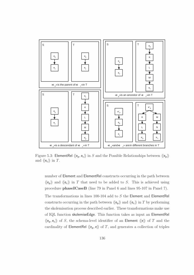
« e p » and « e
c » are in different branches in T
T e’ p
K
S
e’ p
e p
L
e c
M
N
e p e c
« e p » is a descendant of « e
c » in T
T S
e p
e c
e c
K
L
M
e p
« e p » is an ancestor of « e
c » in T
T S
e p
e c
e p
K
L
M
e c
« e p » is the parent of « e
c » in T
T S
e p
e c
e p
e c
Figure 5.3: ElementRel 〈〈ep, ec〉〉 in S and the Possible Relationships between 〈〈ep〉〉and 〈〈ec〉〉 in T .
number of Element and ElementRel constructs occurring in the path between
〈〈ep〉〉 and 〈〈ec〉〉 in T that need to be added to S. This is achieved using
procedure phaseICaseB (line 79 in Panel 6 and lines 95-107 in Panel 7).
The transformations in lines 100-104 add to S the Element and ElementRel
constructs occurring in the path between 〈〈ep〉〉 and 〈〈ec〉〉 in T by performing
the skolemisation process described earlier. These transformations make use
of IQL function skolemiseEdge. This function takes as input an ElementRel
〈〈ep, ec〉〉 of S, the schema-level identifier of an Element 〈〈e〉〉 of T and the
cardinality of ElementRel 〈〈ep, e〉〉 of T , and generates a collection of triples
136

Panel 6: Schema Restructuring Algorithm — Phase I
for every ElementRel 〈〈ep, ec〉〉 in S in a depth-first order do75
if (Table IIa contains a path p in T for ElementRel 〈〈ep, ec〉〉 of S) then76
if (〈〈ep〉〉 is an ancestor of 〈〈ec〉〉 in T ) then77
if (checkConditions(〈〈ep, ec〉〉,p)) then78
phaseICaseB(〈〈ep, ec〉〉,p);79
else if (〈〈ep〉〉 is a descendant of 〈〈ec〉〉 in T ) then80
if (checkConditions(〈〈ep, ec〉〉,p)) then81
let Q :=getInvertedElementRelExtent(〈〈ep〉〉,〈〈ec〉〉);82
phaseICaseB(Q,p);83
else84
// 〈〈ep〉〉 and 〈〈ec〉〉 are located in different branches in Tlet 〈〈e′p〉〉 be the parent of 〈〈ep〉〉 in S;85
if (〈〈e′p〉〉 is a common ancestor of 〈〈ep〉〉 and 〈〈ec〉〉 in T ) then86
let p2 be the path from 〈〈e′p〉〉 to 〈〈ec〉〉 in T ;87
if (checkConditions(〈〈ep, ec〉〉,p2)) then88
let Q := [{x, z}|{x, y} ← 〈〈e′p, ep〉〉; {y, z} ← 〈〈ep, ec〉〉];89
// Q is the extent of virtual ElementRel 〈〈e′p, ec〉〉
phaseICaseB(Q,p2);90
{x, y, z}, where x is an instance of 〈〈ep〉〉, y is an instance of 〈〈e〉〉 and z is an
instance of 〈〈ec〉〉. These triples are used to populate the extents of constructs
〈〈e〉〉, 〈〈ep, e〉〉 and 〈〈e, ec〉〉 of S. More details of function skolemiseEdge are
given later on in this section, where Case (b) is applied to our running
example. Further examples of Case (b) are given in Appendix B.
Lines 105 and 107 then remove the the ElementRel constructs that are the
‘byproducts’ of the skolemisation process. These constructs were added to
S using an ordering of -1 in line 104.2
(c) If 〈〈ep〉〉 is a descendant of 〈〈ec〉〉 in T , we similarly need to add to S the
missing Element and ElementRel constructs to create the path from 〈〈ec〉〉 to
〈〈ep〉〉 (lines 80– 83). We observe that in this case 〈〈ec〉〉 in T is an ancestor
2Using an invalid ordering in this case is not an issue, because the ElementRel constructsusing the invalid ordering are only present in intermediate schemas, and are removed later on.
137

Panel 7: Subroutines for Phase I of the Schema Restructuring Algorithm
/* *********** Function checkConditions(〈〈ep, ec〉〉,p) *********** */
let a = true if all internal Element constructs of path p in T are missing from S ;91
let b = true if ElementRel 〈〈ep, ec〉〉 of S has a 1− n cardinality ;92
let c = true if all ElementRel constructs in p have a 1− 1 cardinality;93
return (a ∧ (¬(b ∧ c)));94
/* ************* Procedure phaseICaseB(〈〈ep, ec〉〉,p) ************* */
let byproducts be an empty list;95
for (each Element 〈〈e〉〉 in p, except for 〈〈ep〉〉 and 〈〈ec〉〉) do96
if (more than one ElementRel construct in p has a 1–n cardinality) then97
Assume that just the first such construct has a 1–n cardinality;98
let card be the cardinality of 〈〈ep, e〉〉 in T ;99
add(〈〈e〉〉,[y|{x, y, z} ← skolemiseEdge 〈〈ep, ec〉〉′e′ card]);100
let i1 be the ordering of 〈〈ep, e〉〉 in T ;101
add(〈〈i1, ep, e〉〉,[{x, y}|{x, y, z} ← skolemiseEdge 〈〈ep, ec〉〉′e′ card]);102
let i2 be the ordering of 〈〈e, ec〉〉 in T , or -1 if 〈〈e, ec〉〉 does not exist in T ;103
add(〈〈i2, e, ec〉〉,[{y, z}|{x, y, z} ← skolemiseEdge 〈〈ep, ec〉〉′e′ card]);104
if (this is not the last iteration) then add 〈〈i2, e, ec〉〉 in byproducts;105
let 〈〈ep〉〉 = 〈〈e〉〉;106
for (each ElementRel 〈〈e, ec〉〉 in byproducts) do contract(〈〈e, ec〉〉,Range Void107
Any);/* ****** Function getInvertedElementRelExtent(〈〈ep〉〉,〈〈ec〉〉) ****** */
// Given ElementRel 〈〈ep, ec〉〉, formulate a query that describes the
// extent of ElementRel 〈〈ec, ep〉〉 with no loss of information.
let Q1 := unnestCollection [Q2|x1← 〈〈ep〉〉], where Q2 is108
if(member [x|{x, y} ← 〈〈ep, ec〉〉] x1)109
[{y, x1}|{x, y} ← 〈〈ep, ec〉〉; x = x1]110
[{generateUID ′ec′ [x1], x1}];111
return Q1;112
/* ******* IQL Function skolemiseEdge(〈〈ep, ec〉〉,’e’,card) ******* */
// card is the cardinality of 〈〈ep, e〉〉 in Tif (card is 1− 1) then113
// Get the distinct instances of 〈〈ep〉〉 participating in 〈〈ep, ec〉〉let q1 := distinct [x|{x, y} ← 〈〈ep, ec〉〉] ;114
// Generate an instance of 〈〈e〉〉 for each of these instances
let q2 := [{x, generateUID ′e′ [x]}|x← q1] ;115
return [{x, y, z}|{x, y} ← q2; {x, z} ← 〈〈ep, ec〉〉];116
else if (card is 1− n) then117
return [{x, generateUID ′e′ [x, z], z}|{x, z} ← 〈〈ep, ec〉〉] ;118
138

of 〈〈ep〉〉. Thus, if we inverted ElementRel 〈〈ep, ec〉〉 to ElementRel 〈〈ec, ep〉〉 in
S, then we could apply procedure phaseICaseB of Case (b) on 〈〈ec, ep〉〉
and the path p from 〈〈ec〉〉 to 〈〈ep〉〉 in T . We also observe that procedure
phaseICaseB does not require an ElementRel to be actually present in S,
but a query describing its extent. Therefore, we do not add 〈〈ec, ep〉〉 to S;
instead, we formulate a query Q that defines its extent, and apply procedure
phaseICaseB to Q and p.
We note that there may be instances of 〈〈ep〉〉 in S with no child instances of
〈〈ec〉〉, and so if we inverted 〈〈ep, ec〉〉 using query [{y, x}|{x, y} ← 〈〈ep, ec〉〉],
then these instances of 〈〈ep〉〉 would be lost. We therefore invert 〈〈ep, ec〉〉
using function getInvertedElementRelExtent (lines 108-112 in Panel 7).
The query formulated by this function prevents the loss of such instances
of 〈〈ep〉〉. In particular, the query iterates through each instance x1 of 〈〈ep〉〉
and checks whether x1 has any child instances of 〈〈ec〉〉. If it does, then the
query returns a list of the instances {x1, y} of 〈〈ep, ec〉〉 that x1 participates
in, by first inverting them to {y, x1}3. Otherwise, if x1 does not have any
child instances of 〈〈ec〉〉, a new tuple {generateUID ′e′c [x1], x1} is generated
as an instance of 〈〈ec, ep〉〉. The XMLDSS-specific IQL function generateUID
is used here to generate a unique instance-level identifier of 〈〈ec〉〉 for each
instance x1 of 〈〈ep〉〉 that does not have a child instance of 〈〈ec〉〉. This
function is further discussed below, together with function skolemiseEdge.
An example of function getInvertedElementRelExtent is given at the end
of Section 5.4.3.
(d) If 〈〈ep〉〉 and 〈〈ec〉〉 are located in different branches in T and the parent
of 〈〈ep〉〉 in S, 〈〈e′p〉〉, is a common ancestor of 〈〈ep〉〉 and 〈〈ec〉〉 in T (as in
the example of Figure 5.3), we need to ensure the existence of two paths
in T within S, p1 from 〈〈e′p〉〉 to 〈〈ep〉〉 and p2 from 〈〈e′p〉〉 to 〈〈ec〉〉. However,
ElementRel 〈〈e′p, ep〉〉 in S will already have been handled in the previous
3Therefore, the query supplied with the transformation returns a list of lists. FunctionunnestCollection col in Panel 7 takes as input a collection and unnests it.
139

step of Phase I, adding path p1 to S (path [e′p, K, L, ep] in the example of
Figure 5.3), and so we only need to add path p2 to S (path [e′p, M, N, ec] in
the example of Figure 5.3).
We observe that in this case S does not contain a single ElementRel construct
that needs to be transformed into a path in T , but rather a path: ElementRel
constructs 〈〈e′p, ep〉〉 and 〈〈ep, ec〉〉 in S correspond to path p2 in T . Similarly
to Case (c), we formulate a query that describes the extent of ElementRel
〈〈e′p, ec〉〉, without any loss of information, and apply Case (b) to transform
〈〈e′p, ec〉〉 to path p2 in T . Lines 84– 90 in Panel 6 list the steps followed in
this case.
We note that if 〈〈e′p〉〉 is not a common ancestor of 〈〈ep〉〉 and 〈〈ec〉〉 in T ,
or if 〈〈e′p〉〉 is not present in T at all, Phase I leaves it to Phase II to add
the missing Element and ElementRel constructs to S with an undetermined
extent, using the query Range Void Any. This is because in such cases there
is a lack of knowledge about how to add to S the Element and ElementRel
constructs of T that it is missing.
Further examples of Case (d) are given in Appendix B.
Running Example
We now illustrate Phase I with respect to our running example. Phase I applied
to Sconf detects that ElementRel construct 〈〈2, author, book〉〉 corresponds to path
[author, item, book] in T , and so Case (b) applies, since 〈〈author〉〉 is an ancestor
of 〈〈book〉〉 in T . The transformations produced are given below, assuming that
the user has supplied cardinality 1 − n for 〈〈2, author, book〉〉 in Sconf , and 1 − n
for 〈〈2, author, item〉〉 and 1−1 for 〈〈1, item, book〉〉 in T . Transformation 20 below
adds to Sconf the missing Element 〈〈item〉〉, while transformations 21 and 22 add
to Sconf ElementRel constructs 〈〈2, author, item〉〉 and 〈〈1, item, book〉〉.
140

20 addEl(〈〈item〉〉, [y|{x, y, z} ← skolemiseEdge 〈〈2, author, book〉〉 ′item′ ′1− n′])
21 addER(〈〈2, author, item〉〉,
[{x, y}|{x, y, z} ← skolemiseEdge 〈〈2, author, book〉〉 ′item′ ′1− n′])
22 addER(〈〈1, item, book〉〉,
[{y, z}|{x, y, z} ← skolemiseEdge 〈〈2, author, book〉〉 ′item′ ′1− n′])
The application of these transformations to the HDM version of the XMLDSS
schema Sconf produces the HDM schema illustrated in Figure 5.4. Applying Phase
I to T in this running example leaves that schema unchanged.
Phase I output
book
root
title
1
1
author
Text
1
genre
2
type
ISBN
1
1
publisher
1
3
birthday
birthmonth
birthyear
name
1
1 2
item
1
2
Figure 5.4: Schema Produced from the Application of Phase I on Sconf .
IQL Functions skolemiseEdge and generateUID
We now give further details of function skolemiseEdge (listed in lines 113-118 in
Panel 7). Consider a source schema S that contains an ElementRel 〈〈ep, ec〉〉 with
cardinality card1, and a target schema that contains ElementRel constructs 〈〈ep, e〉〉
and 〈〈e, ec〉〉 with cardinalities card2 and card3. Assuming S does not contain an
Element 〈〈e〉〉, Phase I will add to S the missing constructs 〈〈e〉〉, 〈〈ep, e〉〉 and 〈〈e, ec〉〉,
using for each one a different projection on the same extent generated by the IQL
function skolemiseEdge. There are are eight different cases to consider, and
141

below we discuss how skolemiseEdge is able to consider just cardinality card2
and generate a correct extent for all eight different cases.
i) The source schema ElementRel 〈〈ep, ec〉〉 has a 1–n cardinality, while both
target schema ElementRel constructs have a 1–1 cardinality. Function skole-
miseEdge is not invoked in this case, since, as discussed earlier in this
section, Phase I considers this case as inconsistent and leaves it to Phase II
to add the missing schema constructs to S with an undetermined extent.
ii) Both target schema ElementRel constructs have a 1–n cardinality. As dis-
cussed earlier in this section, in this case the algorithm considers the first
1–n ElementRel target construct as the one with a 1–n cardinality, and
treats the other one as though it had a 1–1 cardinality. Then, if the source
schema ElementRel 〈〈ep, ec〉〉 has a 1–n cardinality, then this case is reduced
to Case (iii) below. Otherwise, if 〈〈ep, ec〉〉 has a 1–1 cardinality, then this
case is reduced to Case (iv) below.
iii) The source schema ElementRel 〈〈ep, ec〉〉 and the target schema ElementRel
〈〈ep, e〉〉 both have a 1–n cardinality, and ElementRel 〈〈e, ec〉〉 has a 1–1 car-
dinality (see upper left of Figure 5.5). In this case, query Q in line 118 of
Panel 7 guarantees that 〈〈ep, e〉〉 will have a 1–n cardinality and that 〈〈e, ec〉〉
will have a 1–1 cardinality.
This is achieved by generating a new instance for 〈〈e〉〉 for each instance of
〈〈ep, ec〉〉 in S using function generateUID. Since Q iterates through 〈〈ep, ec〉〉,
only instances of 〈〈ep〉〉 with child instances of 〈〈ec〉〉 will be associated with
instances of 〈〈e〉〉. Also, since 〈〈ep, ec〉〉 has a 1–n cardinality, if 〈〈ep, ec〉〉 has
n instances then the unique instances of 〈〈ep〉〉 participating in 〈〈ep, ec〉〉 will
be m ≤ n. Thus, the same instance of 〈〈ep〉〉 may be associated with more
than one instances of 〈〈e〉〉, and so 〈〈ep, e〉〉 will have a 1–n cardinality.
Regarding the cardinality of 〈〈e, ec〉〉, since Q generates n unique instances of
〈〈e〉〉 and since 〈〈ec〉〉 has n unique instances participating in 〈〈ep, ec〉〉, 〈〈e, ec〉〉
will have a 1–1 cardinality. Note that it is not possible for the same instance
142

of 〈〈e〉〉 to be associated with more than one instance of 〈〈ec〉〉 due to the way
Q is formulated.
iv) The source schema ElementRel 〈〈ep, ec〉〉 has a 1–1 cardinality, target schema
ElementRel 〈〈ep, e〉〉 has a 1–n cardinality and ElementRel 〈〈e, ec〉〉 has a 1–1
cardinality (see upper right of Figure 5.5). In this case, the query in line 118
of Panel 7 guarantees that both 〈〈ep, e〉〉 and 〈〈e, ec〉〉 in S will have a 1–1
cardinality, and the explanation is similar to Case (iii).
v) The source schema ElementRel 〈〈ep, ec〉〉 has a 1–n cardinality, target schema
ElementRel 〈〈ep, e〉〉 has a 1–1 cardinality and target schema ElementRel
〈〈e, ec〉〉 has a 1–n cardinality (see bottom left of Figure 5.5). In this case,
the query produced in lines 113-116 of Panel 7 guarantees that 〈〈ep, e〉〉 will
have a 1–1 cardinality, while 〈〈e, ec〉〉 in S will have a 1–n cardinality.
This is achieved by first selecting each instance of 〈〈ep〉〉 that participates in
an instance of 〈〈ep, ec〉〉 (so as not to include instances of 〈〈ep〉〉 with no chil-
dren) and then applying function distinct4 on the result (query q1). Thus,
if there are multiple instances of 〈〈ep, ec〉〉 with the same instance of 〈〈ep〉〉,
only one instance of 〈〈ep〉〉 is selected. We then generate one instance of
〈〈e〉〉 for each instance of 〈〈ep〉〉 that was selected with q1, and then form the
result triples. Thus, if q1 selects n instances of 〈〈ep〉〉, query q2 generates n
instances for 〈〈e〉〉, and so q2 has a 1–1 cardinality. Thus, 〈〈ep, e〉〉 will have
a 1–1 cardinality.
Regarding the cardinality of 〈〈e, ec〉〉, this will be 1–n due to the join in
line 116, which is between q2 (which has a 1–1 cardinality as discussed
above) and 〈〈ep, ec〉〉 (which has a 1–n cardinality).
vi) The source schema ElementRel 〈〈ep, ec〉〉 and the target schema ElementRel
〈〈ep, e〉〉 both have a 1–1 cardinality and ElementRel 〈〈e, ec〉〉 has a 1–n cardi-
nality (see bottom right of Figure 5.5). In this case, the query produced in
4Function distinct removes duplicates from its input list argument by retaining the first oc-currence of each recurring list item. The function does not change the ordering of the remainingitems in the list.
143

Skolemisation Case (iii)
T S
e p
(1-n)
e c
e p
e
T S
e p2 e p1
e c1
e p3
e c3
e c2
e p2
e 1
e c1
e 3
e c3 e c2
e p3 e p1
e c
(1-1)
(1-n)
Skolemisation Case (iv)
T S
e p
(1-1)
e c
e p
e
T S
e p2 e p1
e c1
e p3
e c2
e p2
e 1
e c1
e 2
e c2
e p3 e p1
e c
(1-1)
(1-n)
Skolemisation Case (v)
T S
e p
(1-n)
e c
e p
e
T S
e p2
e p1
e c1
e p3
e c3 e c2
e p2
e 1
e c1
e 2
e c3
e c2
e p3
e p1
e c
(1-n)
(1-1)
Skolemisation Case (vi)
T S
e p
(1-1)
e c
e p
e
T S
e p2
e p1
e c1
e p3
e c2
e p2
e 1
e c1
e 2
e c2
e p3
e p1
e c
(1-n)
(1-1)
e 2
Figure 5.5: Skolemisation Cases (iii)–(vi).
144

lines 113-116 of Panel 7 guarantees that both 〈〈ep, e〉〉 and 〈〈e, ec〉〉 in S will
have a 1–1 cardinality, by a similar argument to Case (v).
vii) All three ElementRel constructs have a 1–1 cardinality. In this case, either
query of function skolemiseEdge can guarantee that 〈〈ep, e〉〉 and 〈〈e, ec〉〉 will
have a 1–1 cardinality, since this case can be seen as a special case of any
one of Cases (ii)-(vi).
In our running example, since the source schema ElementRel 〈〈2, author, book〉〉
has a 1− n cardinality, and the target schema ElementRel 〈〈2, author, item〉〉 has a
1−n cardinality, Case (iii) above applies, and the final query for transformation 20
above is as follows:
[y|{x, y, z} ← [{x, generateUID ′item′ [x, y], y}|{x, y} ← 〈〈2, author, book〉〉]]
which can be rewritten as follows, after unnesting:
[generateUID ′item′ [x, y]|{x, y} ← 〈〈2, author, book〉〉]
We now discuss function generateUID and demonstrate it by example. Note
that, for clarity of explanation, we will be using the full identifiers for Element
and ElementRel constructs, e.g. 〈〈item$1〉〉 and 〈〈2, author$1, book$1〉〉, rather than
the shorthand notation used so far in this chapter. Function generateUID takes
as input an Element identifier, in this case ′item$1′, and a list of instance identi-
fiers, [x, y], and generates an instance identifier of the form elemName$count sid&
instanceCount as follows: the prefix elemName$count is provided by the first ar-
gument, in this case item$1; the sid integer is the same as the sid of each item
in the list provided as the second argument; and the instanceCount is the sum of
the instanceCount of each item in that list. In our running example, if the extent of
〈〈2, author$1, book$1〉〉 was [{author$1 5&1, book$1 5&1}, {author$1 5&1, book$1 5&2}],
then the query above applies the head of the comprehension, generateUID ′item′ [x, y],
once for each instance of the body of the comprehension, which iterates through
the extent of 〈〈2, author, book〉〉. Therefore, generateUID would first be invoked
with arguments ′item$1′ and [author$1 5&1, book$1 5&1], producing item$1 5&2 as
the result, and the second time with the arguments ′item$1′ and [author$1 5&1,
book$1 5&2], producing item$1 5&3 as the result. We observe that the output
145

of generateUID is always the same for the same input, and always different for
different inputs (i.e. it deterministically produces a unique instance identifer for
each unique input).
5.4.3 Phase II - Restructuring
After the completion of Phase I, Phase II is first applied to the source schema S
and then to the target schema T (Phase II is described in Panel 8, while Panel 9
provides details of the procedures invoked in Panel 8).
When Phase I was applied to S, it added to S some of the Element and
ElementRel constructs present in T but not in S; similarly, when Phase I was
applied to T , it added to T some of the Element and ElementRel constructs present
in S but not in T . However, Phase I is not able to resolve all 1-1 structural
incompatibilities between S and T .
The purpose of Phase II is to fully transform the source schema S into the
target schema T — by S and T here we mean the source and target schemas
resulting from the application of Phase I to the original source and target schemas
that were input to the SRA. It does so by adding to S all Element, Attribute and
ElementRel constructs present in T but not in S and then deletes from S all
Element, Attribute and ElementRel constructs present in S but not in T . As
discussed earlier, due to the reversibility of AutoMed primitive transformations,
the same effect can be achieved by adding to S all constructs present in T but
not in S, and then adding to T all constructs present in S but not in T . For
clarity of presentation, we use the terms ‘source’ and ‘target’ in the rest of this
section assuming that Phase II is being applied to S. When Phase II is applied
to T , the terms ‘source’ and ‘target’ should be swapped. This includes references
made to the data structures of Section 5.4.1.
We now discuss the algorithm for Phase II, which is listed in Panels 8 and 9.
When Phase II is applied on S, it first considers every Element in T , in a depth-
first fashion. There are six cases to consider for each Element 〈〈e〉〉 in T , and we
146

discuss these below. In the following, parent(〈〈e〉〉, T ) denotes the parent of 〈〈e〉〉 in
T , parent(〈〈e〉〉, S) denotes the parent of 〈〈e〉〉 in S, and 〈〈p〉〉 denotes the Element
in S that has the same schema-level identifier as parent(〈〈e〉〉, T ) — which may
or may not be the same as parent(〈〈e〉〉, S). Note that parent(〈〈e〉〉, T ) may not
be present in S.
1) If 〈〈e〉〉 is present in S and 〈〈p〉〉 is not, then 〈〈p〉〉 was not originally present in
S but was added to S in the previous step of the algorithm. We therefore add
to S an ElementRel between 〈〈p〉〉 and 〈〈e〉〉 with an extend transformation using
the query Range Void Any (line 122 in Panel 8).
2) If 〈〈e〉〉 is present in S, and is located under the same parent Element (i.e. 〈〈p〉〉=
parent(〈〈e〉〉, S)), then there is an ElementRel 〈〈i, p, e〉〉 in S and an ElementRel
〈〈j, parent(〈〈e〉〉, T), e〉〉 in T .
a) If i = j, then there is nothing to do.
b) If i 6= j, we add 〈〈j, p, e〉〉 to S (line 126 in Panel 8).5
3) If 〈〈e〉〉 is present in S, but is located under a different parent Element than in
T (i.e. 〈〈p〉〉6= parent(〈〈e〉〉, S)), we need to add an ElementRel construct 〈〈p, e〉〉
to S (lines 124 in Panel 8 and 142–160 in Panel 9). Similarly to Phase I, the
way this ElementRel is added to S depends on the relationship between 〈〈p〉〉
and 〈〈e〉〉 in S:
a) If 〈〈p〉〉 is an ancestor of 〈〈e〉〉 in S (line 143), we add 〈〈p, e〉〉 to S using a
path query from 〈〈p〉〉 to 〈〈e〉〉, with no loss of information.
Examples of this case are given at the end of this subsection using our
running example. Further examples are given in Appendix B.
b) If 〈〈p〉〉 is a descendant of 〈〈e〉〉 in S (line 146), and assuming that the user
has not opted for synthetic extent generation (line 147), we add ElementRel
5Note that another child Element 〈〈e′〉〉 of 〈〈p〉〉 may be in the same position j. This is not aproblem, because 〈〈e′〉〉 will either be removed or moved to another position when Phase II isapplied to T .
147

〈〈p, e〉〉 to S, using a path query from 〈〈p〉〉 to 〈〈e〉〉 in S. This could lead to
loss of information, since there may be instances of 〈〈e〉〉 in S that do not
have descendant instances of 〈〈p〉〉.
If the user has opted for synthetic extent generation, then we add 〈〈p, e〉〉 to
S using a query produced by function getInvertedElementRelExtent, de-
fined in Panel 7 of Section 5.4.2 for Phase I, which ensures that no instances
of 〈〈p〉〉 are lost (line 150).
We recall that function getInvertedElementRelExtent as defined in Phase
I is able to derive the extent of an ElementRel 〈〈ec, ep〉〉, given an ElementRel
〈〈ep, ec〉〉. However, it is trivial to extend it to be able to derive the extent of
an ElementRel 〈〈ec, ep〉〉, given an Element 〈〈ec〉〉 that is the descendant of an
Element 〈〈ep〉〉. This is achieved by replacing ElementRel 〈〈ep, ec〉〉 in lines 109
and 110 of Panel 7 with the path query from 〈〈ep〉〉 to 〈〈ec〉〉 and projecting
on these two Element constructs (see Appendix B for this definition).
Examples of this case are given at the end of this subsection, where it is ap-
plied to our running example. Further examples are given in Appendix B.
c) If 〈〈p〉〉 and 〈〈e〉〉 are located in different branches in S (lines 152-160 in
Panel 9), and assuming that the user has opted to not allow synthetic
extent generation, we add ElementRel 〈〈p, e〉〉 to S, using a path query from
〈〈p〉〉 to 〈〈e〉〉 through the lowest common ancestor of 〈〈p〉〉 and 〈〈e〉〉 in S,
〈〈ea〉〉. Similarly to Case (2b), this could lead to loss of information, since
there may be instances of 〈〈ea〉〉 that do not have descendant instances of
〈〈p〉〉.
If the user has opted to allow synthetic extent generation, we similarly add
〈〈p, e〉〉 using a path query from 〈〈p〉〉 to 〈〈e〉〉 through 〈〈ea〉〉, but this time we
use function getInvertedElementRelExtent (line 159) to derive the path
query from 〈〈p〉〉 to 〈〈ea〉〉. This ensures that no loss of information occurs.
Examples of this case are given in Appendix B.
4) If 〈〈e〉〉 is not present in S and 〈〈p〉〉 is null, then 〈〈p〉〉 was not originally present in
S but was added to S in the previous step of the algorithm. We therefore add to
148
S 〈〈e〉〉 and an ElementRel between 〈〈p〉〉 and 〈〈e〉〉 with extend transformations
using the query Range Void Any (line 129 in Panel 8 and lines 167–168 in
Panel 9).
5) If 〈〈e〉〉 is not present in S, it may be possible to add it to S with an attribute-
to-element transformation under certain conditions. In particular, if 〈〈e〉〉 is
not present in S, but 〈〈p〉〉 in S has an attribute 〈〈p, a〉〉, such that the label of a
is equivalent to the label of 〈〈e〉〉 in T , and T contains an ElementRel 〈〈e, Text〉〉,
then an attribute-to-element transformation is performed. This transformation
adds to S constructs 〈〈e〉〉, 〈〈i, p, e〉〉 (where i is the position of 〈〈e〉〉 in the list of
children of parent(〈〈e〉〉, T )) and 〈〈j, e, Text〉〉 (where j is the position of 〈〈Text〉〉
in the list of children of 〈〈e〉〉). The extents of these constructs are defined with
the help of function skolemiseEdge6 (line 132 in Panel 8 and lines 161–165
in Panel 9).
Examples of this case are given at the end of this subsection and in Appendix B.
6) If 〈〈e〉〉 is not present in S, and 〈〈p〉〉 in S does not have such an Attribute
〈〈p, a〉〉 or T does not contain an ElementRel 〈〈e, Text〉〉, we add to S 〈〈e〉〉 and an
ElementRel between 〈〈p〉〉 and 〈〈e〉〉 with extend transformations using the query
Range Void Any (line 133 in Panel 8 and lines 167–168 in Panel 9).
Examples of this case are given at the end of this subsection and in Appendix B.
Phase II next processes the attributes of 〈〈e〉〉 in T (lines 134–136 in Panel 8)
similarly to elements, in that if an attribute ai of 〈〈e〉〉 in T is not present as an
attribute of 〈〈e〉〉 in S, an element-to-attribute transformation is first attempted
(lines 135 and 169): if 〈〈e〉〉 in S has a child element 〈〈c〉〉 with the same label
as 〈〈ai〉〉 (i.e. if S contains ElementRel 〈〈e, c〉〉), and if 〈〈c〉〉 has a child text node
(i.e. if S contains ElementRel 〈〈c, Text〉〉), then 〈〈e, ai〉〉 is added to S with a query
that uses the extents of 〈〈e, c〉〉 and 〈〈e, Text〉〉 to populate 〈〈e, ai〉〉. Otherwise the
6In this case, skolemiseEdge takes as input an Attribute 〈〈p, a〉〉 and a string e (the schema-level identifier of the Element to be produced by the attribute-to-element transformation), andfor each tuple {x, y} in the extent of 〈〈p, a〉〉 generates a tuple {x, z, y}, where z is an instance-levelidentifier for 〈〈e〉〉.
149

Panel 8: Schema Restructuring Algorithm — Phase II
for every element 〈〈e〉〉 in T in a depth-first order: do119
/* ******************** Handle Element ********************* */
let 〈〈p〉〉 be the element with the same label as parent(〈〈e〉〉, T ) in S;120
if (〈〈e〉〉 is present in S) then121
if (〈〈p〉〉 is not present in S and the ordering of 〈〈e〉〉 under 〈〈p〉〉 in T is j)122
then extend(〈〈j, p, e〉〉,Range Void Any);else if (〈〈p〉〉 6= parent(〈〈e〉〉, S)) then123
InsertElementRel(〈〈p〉〉,〈〈e〉〉)124
else if (the ordering of 〈〈e〉〉 under 〈〈p〉〉 is i in S, j in T , and i 6= j) then125
add(〈〈j, p, e〉〉,〈〈i, p, e〉〉);126
else127
/* if 〈〈e〉〉 is not present in S */
if (〈〈p〉〉 is not present in S) then128
AddElementAndElementRel(〈〈e〉〉,〈〈p〉〉);129
else if (〈〈e〉〉 in T has a child text node and 〈〈p〉〉 has an attribute 〈〈p, a〉〉,130
with the same label as 〈〈e〉〉 in T ) thenlet c be the cardinality of ElementRel 〈〈parent(〈〈e〉〉,T), e〉〉 in T ;131
Attribute2Element(〈〈p, a〉〉,〈〈e〉〉,c)132
else AddElementAndElementRel(〈〈e〉〉,〈〈p〉〉)133
/* ******************* Handle Attributes ******************* */
for (every attribute ai of 〈〈e〉〉 in T not present in 〈〈e〉〉 in S) do134
if (〈〈e〉〉 in S has a child element 〈〈c〉〉 with the same label as ai and 〈〈c〉〉135
has a child text node) then Element2Attribute(ai,〈〈e〉〉,〈〈c〉〉)else AddAttribute(〈〈e〉〉,ai)136
/* ******************* Handle Text Nodes ******************* */
if (T has an ElementRel 〈〈j, e,Text〉〉) then137
if (〈〈e〉〉 in S does not have an ElementRel to the Text node) then138
extend(〈〈j, e,Text〉〉,Range Void Any);139
else if (S has an ElementRel 〈〈i, e,Text〉〉 and i 6= j) then140
add(〈〈j, e,Text〉〉,〈〈i, e,Text〉〉);141
attribute is inserted with an extend transformation, using the query Range Void
Any (lines 136 and 170). This time, a synthetic extent is not generated for the
attribute, even if the user has opted for synthetic extent generation, as missing
attribute instances cannot cause further loss of source data.
150

Panel 9: Subroutines for Phase II of Schema Restructuring Algorithm
/* *********** Proc1: InsertElementRel(〈〈p〉〉,〈〈e〉〉) ************** */
let i be the position of 〈〈e〉〉 in the list of children of parent(〈〈e〉〉, T );142
if (〈〈p〉〉 is an ancestor of 〈〈e〉〉) then143
let 〈〈ej〉〉 be the elements in the path from 〈〈p〉〉 to 〈〈e〉〉 in S, 1 ≤ j ≤ m;144
add(〈〈i, p, e〉〉,[{x, y}|{x, d1} ← 〈〈p, e1〉〉; . . . ; {dm, y} ← 〈〈em, e〉〉]);145
else if (〈〈p〉〉 is a descendant of 〈〈e〉〉) then146
if (synthetic extent generation is not permitted) then147
let 〈〈ek〉〉 be the elements in the path from 〈〈e〉〉 to 〈〈p〉〉 in S, 1 ≤ k ≤ n;148
let Q = [{y, x}|{x, u1} ← 〈〈e, e1〉〉; . . . ; {un, y} ← 〈〈en, p〉〉];149
else let Q := getInvertedElementRelExtent(〈〈e〉〉, 〈〈p〉〉);150
add(〈〈i, p, e〉〉,Q)151
else152
// 〈〈p〉〉 and 〈〈e〉〉 are in different branches
let 〈〈ea〉〉 be the common ancestor of 〈〈p〉〉 and 〈〈e〉〉 in S;153
let 〈〈ek〉〉 be the elements in the path from 〈〈ea〉〉 to 〈〈p〉〉 in S, 1 ≤ k ≤ n;154
let 〈〈e′j〉〉 be the elements in the path from 〈〈ea〉〉 to 〈〈e〉〉 in S, 1 ≤ j ≤ m;155
// Associate 〈〈ea〉〉 and 〈〈e〉〉 using the path between them
let Q1 = [{x, y}|{x, d1} ← 〈〈ea, e′
1〉〉; . . . ; {dm, y} ← 〈〈e′m, e〉〉]] ;156
if (synthetic extent generation is not permitted) then157
// Associate 〈〈ea〉〉 and 〈〈p〉〉 using the path between them
let Q2 = [{y, x}|{x, u1} ← 〈〈ea, e1〉〉; . . . ; {un, y} ← 〈〈en, p〉〉] ;158
else let Q2 :=getInvertedElementRelExtent(〈〈ea〉〉,〈〈p〉〉);159
add(〈〈i, p, e〉〉,[{x, z}|{x, y} ← Q2; {y, z} ← Q1]);160
/* ********** Proc2: Attribute2Element(〈〈p, a〉〉,〈〈e〉〉,c) ********** */
let i be the position of 〈〈e〉〉 in the list of children of parent(〈〈e〉〉, T );161
let j be the position of 〈〈Text〉〉 in the list of children of 〈〈e〉〉 in T ;162
addEl(〈〈e〉〉,[y|{x, y, z} ← skolemiseEdge 〈〈p, a〉〉 ′e′ c]);163
addER(〈〈i, p, e〉〉,[{x, y}|{x, y, z} ← skolemiseEdge 〈〈p, a〉〉 ′e′ c]);164
addER(〈〈j, e,Text〉〉,[{y, z}|{x, y, z} ← skolemiseEdge 〈〈p, a〉〉 ′e′ c]);165
/* ********* Proc3: AddElementAndElementRel(〈〈e〉〉,〈〈p〉〉) ********* */
let i be the position of 〈〈e〉〉 in the list of children of parent(〈〈e〉〉, T );166
extendEl(〈〈e〉〉,Range Void Any);167
extendER(〈〈i, p, e〉〉,Range Void Any);168
/* *********** Proc4: Element2Attribute(a,〈〈e〉〉,〈〈c〉〉) *********** */
addAtt(〈〈e, a〉〉,[{x,z}|{x,y}←〈〈e, c〉〉;{y,z}←〈〈c,Text〉〉]);169
/* *************** Proc5: AddAttribute(〈〈e〉〉,a) **************** */
extendAtt(〈〈e, a〉〉,Range Void Any);170
151

Finally, if 〈〈e〉〉 in T has a child text node (i.e. T contains ElementRel 〈〈j, e, Text〉〉,
for some j) and 〈〈e〉〉 in S does not, we add an ElementRel 〈〈j, e, Text〉〉 to 〈〈e〉〉 in
S, using the query Range Void Any (line 139). If 〈〈e〉〉 in S contains an ElementRel
〈〈i, e, Text〉〉, but i 6= j, 〈〈j, e, Text〉〉 is added to S using the extent of 〈〈i, e, Text〉〉
(line 141).
We note that line 124 in Panel 8 simulates a ‘move’ operation. When Phase
II is applied on S, line 124 inserts an ElementRel from 〈〈p〉〉 to 〈〈e〉〉 in S. When
Phase II is applied on T , line 124 inserts an ElementRel from the Element with the
same label as parent(〈〈e〉〉, S) in T to 〈〈e〉〉 in T . When traversing the transforma-
tion pathway S ↔ T in the direction S → T , this latter insertion represents the
removal of ElementRel 〈〈parent(〈〈e〉〉, S), e〉〉 from S. These two transformations
therefore perform a ‘move’ operation on S, moving the subtree rooted at 〈〈e〉〉
from under parent(〈〈e〉〉, S) to under 〈〈p〉〉. Instead of regenerating the subtree
rooted at 〈〈e〉〉 to under 〈〈p〉〉 and then removing the subtree rooted at 〈〈e〉〉 from
under parent(〈〈e〉〉, S), the algorithm simply inserts an ElementRel between 〈〈p〉〉
and 〈〈e〉〉, and then removes the ElementRel between parent(〈〈e〉〉, S) and 〈〈e〉〉. This
results in a transformation pathway that is possibly much shorter (depending on
the constructs comprising the subtree rooted at 〈〈e〉〉 in S). This is significant,
because the I/O cost of storing the transformations in the AutoMed Repository
(in a DBMS on disk) is expected to be far greater than the running time of the
SRA.
Running Example
Referring to our running example, the application of Phase II on the schema
output by Phase I (see Figure 5.4) produces transformations 23 – 29 listed below.
The resulting schema Sres is illustrated in Figure 5.6 (grey denotes constructs
existing before the application of Phase II, black denotes constructs added by
Phase II).
152

23 addER(〈〈1, root, author〉〉,
[{x, y}|{x, d1} ← 〈〈1, root, genre〉〉; {d1, y} ← 〈〈1, genre, author〉〉])
24 addAtt(〈〈book, ISBN〉〉,[{x,z}|{x,y}←〈〈1, book, ISBN〉〉;{y,z}←〈〈1, ISBN,Text〉〉])
25 addER(〈〈1, book, title〉〉,〈〈2, book, title〉〉)
26 extendEl(〈〈year〉〉, Range Void Any)
27 extendER(〈〈2, book, year〉〉, Range Void Any)
28 extendER(〈〈1, year,Text〉〉,Range Void Any)
29 addER(〈〈3, book, genre〉〉,unnestCollection [Q1|x1← 〈〈genre〉〉])
where in 29 Q1 is
if(member [x|{x, y} ← path1] x1) [{y, x}|{x, y} ← path1; x = x1]
[{generateUID ′book ′ [x1], x1}]
and path1 = [{p1, p3}|{p1, p2} ← 〈〈1, genre, author〉〉; {p2, p3} ← 〈〈2, author, book〉〉]
The application of Phase II on schema T produces transformations 30 – 39
listed below, and the resulting schema Tres is illustrated in Figure 5.6:
30 addER(〈〈1, root, genre〉〉,
[{x, y}|{x, d1} ← 〈〈1, root, author〉〉; {d1, d2} ← 〈〈2, author, item〉〉;
{d2, d3} ← 〈〈1, item, book〉〉; {d3, y} ← 〈〈3, book, genre〉〉])
31 addER(〈〈1, genre, author〉〉,unnestCollection [Q2|x← 〈〈genre〉〉])
32 addER(〈〈2, author, book〉〉,
[{x, y}|{x, d1} ← 〈〈2, author, item〉〉; {d1, y} ← 〈〈1, item, book〉〉])
33 addEl(〈〈ISBN〉〉, [y|{x, y, z} ← skolemiseEdge 〈〈book, ISBN〉〉 ′ISBN′ ′1− 1′])
34 addER(〈〈1, book, ISBN〉〉,
[{x, y}|{x, y, z} ← skolemiseEdge 〈〈book, ISBN〉〉 ′ISBN′ ′1− 1′])
35 addER(〈〈1, ISBN,Text〉〉,
[{y, z}|{x, y, z} ← skolemiseEdge 〈〈book, ISBN〉〉 ′ISBN′ ′1− 1′])
36 addER(〈〈2, book, title〉〉,〈〈1, book, title〉〉)
37 extendEl(〈〈publisher〉〉,Range Void Any)
38 extendER(〈〈3, book, publisher〉〉,Range Void Any)
39 extendER(〈〈1, publisher,Text〉〉,Range Void Any)
where in 31 Q2 is
153

T res
1
1
S res
book
root
title
1
1
author
Text
1
genre
2
type
ISBN
1
1
publisher
1
3
birthday
birthmonth
birthyear
name
1
1 2
item
1
1
ISBN 2
1
year
author
Text
name
1
1
birthday
birthmonth
birthyear
root
1
book
genre
3
title
1
1
ISBN
type year
2
1
1
item
2
1
publisher
3
ISBN
1 1
1
2
3
1 2
Figure 5.6: Identical Schemas Sres and Tres.
if(member [x|{x, y} ← path2] x) [{y, x}|{x, y} ← path2; x = x1]
[{generateUID ′author ′ [x1], x1}]
and path2 = [{p1, p4}|{p4, p3} ← 〈〈2, author, item〉〉; {p3, p2} ← 〈〈1, item, book〉〉;
{p2, p1} ← 〈〈3, book, genre〉〉]
Figure 5.7 illustrates our running example after the application of the entire
SRA. Numbers in white circles denote transformations produced by the SRA,
while numbers in grey circles denote their reverse transformations.
S S conf data
source
id S res T res T data
source 20 29
20 29
39 30
39 30
Figure 5.7: Running Example after Application of the SRA.
We list below the overall sequence of primitive transformations comprising
the pathways Sconf → Sres and Tres → T . These illustrate how the two phases
of the SRA first augment Sconf with all the constructs of T that Sconf does not
contain, and how the resulting schema Sres is then reduced by removing those
constructs not present in T . We note that transformations 39 – 30 listed below
154

(Tres → T ) are the reverse of the transformations 30 – 39 listed above (T → Tres).
Also, we do not list the id transformations between Sres and Tres, which actually
occur between transformations 29 and 39 .
We see that transformations 20 - 22 skolemise ElementRel 〈〈2, author, book〉〉,
adding constructs 〈〈item〉〉, 〈〈2, author, item〉〉 and 〈〈1, item, book〉〉, while transfor-
mation 32 deletes ElementRel 〈〈2, author, book〉〉. Transformation 23 adds Ele-
mentRel 〈〈1, root, author〉〉, and this, together with transformation 31 , moves the
subtree with root Element 〈〈author〉〉 under 〈〈root〉〉. Transformation 24 performs
an element-to-attribute transformation, using constructs 〈〈1, book, ISBN〉〉 and
〈〈1, ISBN, Text〉〉 to populate the extent of new attribute 〈〈book, ISBN〉〉. This trans-
formation is complemented by transformations 35 – 33 , which delete constructs
〈〈1, book, ISBN〉〉, 〈〈1, ISBN, Text〉〉 and 〈〈ISBN〉〉 (the reverse transformations, 33 –
35 , perform an attribute-to-element transformation in T ). Next, 25 and 36
change the order of ElementRel 〈〈2, book, title〉〉 under 〈〈book〉〉. Then transfor-
mations 26 – 28 add constructs 〈〈year〉〉, 〈〈2, book, year〉〉 and 〈〈1, year, Text〉〉 using
the query Range Void Any, since no information is available from S about their
extents. Another move operation is performed by transformations 29 and 30 ,
which move the subtree with root Element 〈〈genre〉〉 under 〈〈book〉〉. Finally,
transformations 39 - 37 delete constructs 〈〈publisher〉〉, 〈〈3, book, publisher〉〉 and
〈〈1, publisher, Text〉〉 using the query Range Void Any, since their extents cannot be
derived by the rest of the schema constructs of S.
20 addEl(〈〈item〉〉, [y|{x, y, z} ← skolemiseEdge 〈〈2, author, book〉〉 ′item′ ′1− n′])
21 addER(〈〈2, author, item〉〉,
[{x, y}|{x, y, z} ← skolemiseEdge 〈〈2, author, book〉〉 ′item′ ′1− n′])
22 addER(〈〈1, item, book〉〉,
[{y, z}|{x, y, z} ← skolemiseEdge 〈〈2, author, book〉〉 ′item′ ′1− n′])
23 addER(〈〈1, root, author〉〉,
[{x, y}|{x, d1} ← 〈〈1, root, genre〉〉; {d1, y} ← 〈〈1, genre, author〉〉])
24 addAtt(〈〈book, ISBN〉〉,[{x,z}|{x,y}←〈〈1, book, ISBN〉〉;{y,z}←〈〈1, ISBN,Text〉〉])
25 addER(〈〈1, book, title〉〉,〈〈2, book, title〉〉)
26 extendEl(〈〈year〉〉, Range Void Any)
155

27 extendER(〈〈2, book, year〉〉, Range Void Any)
28 extendER(〈〈1, year,Text〉〉,Range Void Any)
29 addER(〈〈3, book, genre〉〉,unnestCollection [Q1|x← 〈〈genre〉〉])
39 contractER(〈〈1, publisher,Text〉〉,Range Void Any)
38 contractER(〈〈3, book, publisher〉〉,Range Void Any)
37 contractEl(〈〈publisher〉〉,Range Void Any)
36 deleteER(〈〈2, book, title〉〉,〈〈1, book, title〉〉)
35 deleteER(〈〈1, ISBN,Text〉〉,
[{y, z}|{x, y, z} ← skolemiseEdge 〈〈book, ISBN〉〉 ′ISBN′ ′1− 1′])
34 deleteER(〈〈1, book, ISBN〉〉,
[{x, y}|{x, y, z} ← skolemiseEdge 〈〈book, ISBN〉〉 ′ISBN′ ′1− 1′])
33 deleteEl(〈〈ISBN〉〉, [y|{x, y, z} ← skolemiseEdge 〈〈book, ISBN〉〉 ′ISBN′ ′1− 1′])
32 deleteER(〈〈2, author, book〉〉,
[{x, y}|{x, d1} ← 〈〈2, author, item〉〉; {d1, y} ← 〈〈1, item, book〉〉])
31 deleteER(〈〈1, genre, author〉〉,unnestCollection [Q2|x← 〈〈genre〉〉])
30 deleteER(〈〈1, root, genre〉〉,
[{x, y}|{x, d1} ← 〈〈1, root, author〉〉; {d1, d2} ← 〈〈2, author, item〉〉;
{d2, d3} ← 〈〈1, item, book〉〉; {d3, y} ← 〈〈3, book, genre〉〉])
where in 29 Q1 is
if(member [x|{x, y} ← path1] x1) [{y, x}|{x, y} ← path1; x = x1]
[{generateUID ′book ′ [x1], x1}]
and path1 = [{p1, p3}|{p1, p2} ← 〈〈1, genre, author〉〉; {p2, p3} ← 〈〈2, author, book〉〉]
and where in 31 Q2 is
if(member [x|{x, y} ← path2] x1) [{y, x}|{x, y} ← path2; x = x1]
[{generateUID ′author ′ [x1], x1}]
and path2 = [{p1, p4}|{p4, p3} ← 〈〈2, author, item〉〉; {p3, p2} ← 〈〈1, item, book〉〉;
{p2, p1} ← 〈〈3, book, genre〉〉]
5.4.4 Correctness of the SRA
We now illustrate the correctness of the SRA using our running example: we refer
the reader to Appendix B for a detailed discussion of the correctness of the SRA.
We recall from Chapter 4 that the pathway Sconf ↔ T produced by the SRA in a
156

peer-to-peer transformation setting is considered as being correct if Sconf and T
are behaviourally consistent. To show this, we need to show that for any query
QS on Sconf , the results of Q′
S are contained in the results of QS, where Q′
S is
produced by rewriting QS on S to QT on T , using GAV reformulation and path-
way Sconf → T , and then rewriting QT to Q′
S on Sconf , using GAV reformulation
and pathway T → Sconf . If the results of QS and Q′
S are equivalent, then Sconf
and T are behaviourally equivalent with respect to query QS.
Example 1. Consider query QS = 〈〈2, author, book〉〉 on Sconf . Using transforma-
tion 32 , QS is rewritten on T as QT =[{x, y}|{x, d1} ← 〈〈2, author, item〉〉; {d1, y} ←
〈〈1, item, book〉〉]. Using transformations 21 and 22 , QT is rewritten to Q′
S on Sconf
as follows:
Q′
S =[{x, y}|
{x, d1} ← [{x, y}|{x, y, z} ← skolemiseEdge 〈〈2, author, book〉〉 ′item′ ′1− n′];
{d1, y} ← [{y, z}|{x, y, z} ← skolemiseEdge 〈〈2, author, book〉〉 ′item′ ′1− n′]]
Applying list comprehension unnesting, this simplifies to:
Q′
S =[{x, y}|{x, d1, z} ← skolemiseEdge 〈〈2, author, book〉〉 ′item′ ′1− n′;
{x1, d1, y} ← skolemiseEdge 〈〈2, author, book〉〉 ′item′ ′1− n′]
Since function skolemiseEdge will always yield the same result given the same
input, and since the two generators in the above comprehension are joined on
variable d1, the other two pairs of variables must be equal, i.e. x=x1 and z=y for
all tuples generated by the comprehension. Therefore, Q′
S can be simplified to:
Q′
S =[{x, y}|{x, d1, y} ← skolemiseEdge 〈〈2, author, book〉〉 ′item′ ′1− n′]
which is equivalent to:
Q′
S =[{x, y}|{x, d1, y} ← skolemiseEdge QS′item′ ′1− n′]
We know from the definition of skolemiseEdge that the function generates as
many instances as the instances of its ElementRel (or Attribute) argument (in this
case QS), and we also know that it does not alter the first and third items in the
triples that it produces, and so QS ≡ Q′
S.
Assuming now that the user had not permitted synthetic extent generation,
then QT would be the same as above, but Q′
S would be equal to the empty list,
157

and so it is trivially the case that Q′
S ⊆ QS.
Example 2. As a second example, consider query
QS =[{x, z}|{x, y} ← 〈〈1, book, ISBN〉〉; {y, z} ← 〈〈1, ISBN, Text〉〉]
on S, which gives us the opportunity to examine the correctness of the element-
to-attribute transformation of the SRA. Using transformations 34 and 35 , QS is
rewritten to the following query on T :
QT =[{x, z}|
{x, y} ← [{x, y}|{x, y, z} ← skolemiseEdge 〈〈book, ISBN〉〉 ′ISBN′ ′1− 1′];
{y, z} ← [{y, z}|{x, y, z} ← skolemiseEdge 〈〈book, ISBN〉〉 ′ISBN′ ′1− 1′]]
Applying list comprehension unnesting, this simplifies to:
QT =[{x, z}|{x, y, z1} ← skolemiseEdge 〈〈book, ISBN〉〉 ′ISBN′ ′1− 1′;
{x1, y, z} ← skolemiseEdge 〈〈book, ISBN〉〉 ′ISBN′ ′1− 1′]
As in the previous example, since both instances of skolemiseEdge in QT have
the same arguments, and since they are joined on variable y, the other two pairs
of variables must be equal, i.e. x=x1 and z1=z, and so Q′
S can be simplified to:
QT =[{x, z}|{x, y, z} ← skolemiseEdge 〈〈book, ISBN〉〉 ′ISBN′ ′1− 1′]
Using transformation 24 , QT is rewritten to Q′
S on S as follows:
Q′
S =[{x, z}|{x, y, z} ← skolemiseEdge
[{x, z}|{x, y} ← 〈〈1, book, ISBN〉〉; {y, z} ← 〈〈1, ISBN,Text〉〉] ′ISBN′ ′1− 1′]
or, since the first argument of skolemiseEdge is the original query QS:
Q′
S =[{x, z}|{x, y, z} ← skolemiseEdge QS′ISBN′ ′1− 1′]
By a similar argument to Example 1, QS ≡ Q′
S, or Q′
S ⊆ QS if the user had
not permitted synthetic extent generation.
5.4.5 Complexity Analysis of the SRA
We now examine the complexity of the SRA by deriving the complexity of each
of its three phases. In our discussion, we consider only the complexity of the SRA
and not of the AutoMed API, i.e. we assume that the complexity of applying any
AutoMed primitive transformation to a schema is the same and is O(1).
158

Complexity of the Initialisation Phase
When applied to the source schema S, the Initialisation Phase traverses S and
creates pointers to each Element and Attribute construct of S. The complexity of
this process is O(ES) + O(AS), where ES is the number of Element constructs of
S and AS is the number of Attribute constructs of S. Similarly, when applied to
the target schema T , the Initialisation Phase traverses T and creates pointers to
each Element and Attribute construct of T , and the complexity of this process is
O(ET ) + O(AT ).
The Initialisation Phase also traverses S one more time, considers each Ele-
mentRel construct of S and locates the corresponding path in T , if such a path
exists. The complexity of locating a path in T is, in the worst case, O(2 hT ),
where hT is the height of T , if the start and end nodes of the path are both
leaf nodes and that their lowest common ancestor is the root. Thus, the worst
case complexity for this process for S is O(RS hT ), where RS is the number of
ElementRel constructs of S. However, in any tree the number of edges is one less
than the number of its nodes, and so this can also be expressed as O(ES hT ). By
a similar argument, the complexity of this process when the Initialisation Phase
is applied to T is O(ET hS).
The overall worst-case complexity of the Initialisation Phase for S is the sum
of the complexities discussed above, i.e.
O(ES + ET )+O(AS + AT )+O(ES hT )+O(ET hS)
Complexity of Phase I
When applied to S, the Initialisation Phase produces a correspondence between
each ElementRel construct 〈〈ep, ec〉〉 in S and the corresponding path pT in T .
When applied to S, Phase I handles each such pair (〈〈ep, ec〉〉, pT ). Assuming a
complexity CS for handling each such pair, and assuming that every ElementRel
in S has a corresponding path in T , the complexity of Phase I for S is O(ES CS).
Similarly, the complexity of Phase I for T is O(ET CT ). We now discuss com-
plexity CS (and CT ).
159

As discussed in Section 5.4.2, there are four cases to consider for pair (〈〈ep, ec〉〉,
pT ): (a) 〈〈ep〉〉 is the parent of 〈〈ec〉〉 in T , (b) 〈〈ep〉〉 is an ancestor of 〈〈ec〉〉 in T , (c)
〈〈ep〉〉 is a descendant of 〈〈ec〉〉 in T , and (d) 〈〈ep〉〉 and 〈〈ec〉〉 are located in different
branches in T .
Phase I does not need to do anything for Case (a), and so the complexity for
this case is O(1).
When handling Case (b), Phase I considers each Element in pT and adds
three constructs to S. In the worst case, pT is a path from a leaf node to the
root, and therefore the complexity of processing each Element in pT is O(hTC ′
S),
where C ′
S is the complexity of issuing the three transformations. Each of these
transformations has a constant complexity (since none of the queries supplied
with the transformations are path queries) — so the complexity of processing
pT is O(hT ). Finally, Phase I deletes the ‘byproduct’ ElementRel constructs it
produced, which are one less than the total number of ElementRel constructs in
pT — this also has a complexity of O(hT ). Thus, Case (b) of Phase I has an
overall worst-case complexity O(2 hT ).
Case (c) is similar to Case (b), but first invokes function getInvertedElemen-
tRelExtent that formulates a query whose length is, in the worst case, equal to
the height of T . Therefore, the worst-case complexity of Case (c) is O(3 hT ).
Case (d) is similar to Case (c), but in this case the query is derived using a
path query of length 2, and so the worst-case complexity of Case (d) is O(2 hT ).
Therefore, the overall worst-case complexity of Phase I for S and T is:
O(ES hT ) + O(ET hS)
Complexity of Phase II
When applied to S (respectively, T ), Phase II traverses T (S), considering each
Element, Attribute and ElementRel construct in T (S), and issues AutoMed trans-
formations on S (T ), depending on whether or not the constructs of T (S) are
present in S (T ). The queries supplied with the transformations that add Element
and Attribute constructs, as well as with those that add ElementRel constructs to
160

the Text construct, are non-path queries, and therefore the complexity of gener-
ating each of them is O(1). A query supplied with a transformation that adds an
ElementRel construct (other than to the Text construct) is a path query. Assuming
complexity CS (CT ) for deriving such a query in S (T ), the overall complexity of
Phase II is O(ES +ET ) + O(AS +AT ) + O(ESCS) + O(ETCT ). We now discuss
complexity CS (and CT ).
Phase II handles the addition of an ElementRel construct 〈〈ep, ec〉〉 of T to S
depending on the relationship of 〈〈ep〉〉 and 〈〈ec〉〉 in S. If 〈〈ep〉〉 and 〈〈ec〉〉 have an
ancestor-descendant or a descendant-ancestor relationship, then a path query is
supplied with the AutoMed transformation, and deriving this query has a worst-
case complexity of O(hS).
If 〈〈ep〉〉 and 〈〈ec〉〉 are in leaves of different branches in S, then Phase II issues
a transformation supplied with a query that contains two path queries. The
complexity of deriving each of these queries is, in the worst case, O(hS), so CS is
O(hS). Similarly, CT is O(hT ) in the worst case.
Therefore, the overall worst-case complexity of Phase II is:
O(ES + ET ) + O(AS + AT ) + O(ES hT ) + O(ET hS)
Overall Complexity
Combining the complexities of each of the three phases, the overall worst-case
complexity for the SRA is
O(ES + ET ) + O(AS + AT ) + O(ES hT ) + O(ET hS)
Based on our earlier discussion, the actual complexity of the SRA depends
on the number of elements and attributes of the source and target schemas (but
not on the elements’ “fan-out”), and on the number and the length of the path
queries produced. Since it is not possible to know the number and length of the
path queries that are produced by the SRA for an arbitrary pair of schemas S
and T , we have assumed here that, in the worst case, a path query is generated
for each ElementRel construct of S and T , and that the length of each path query
on S (T ) is, in the worst-case, twice the height of T (S).
161

5.5 Schema Integration Algorithms
Consider now the integration of a number of XML data sources with schemas
LS1 . . . LSn under a global schema GS. As discussed in Chapter 4, our approach
supports two types of schema integration in such cases: top-down, in which a
fixed global schema is predefined, and bottom-up, in which the global schema is
automatically generated. We now discuss these two types of integration in more
detail, and provide pseudocode for the respective algorithms (implementation of
these algorithms is an area of future work).
As shown in Panel 10, given our schema restructuring algorithm described in
Section 5.4, and assuming that schema conformance has already been performed,
top-down integration is straightforward: each conformed data source schema is
restructured to match the structure of the predefined global schema. This type
of integration is preferable in settings where a specific global schema needs to be
enforced and where there is no strict requirement to preserve all the information
contained in the data sources. We note that, given the worst-case complexity
of the SRA presented in Section 5.4.5, the worst-case complexity of top-down
schema integration is:
O(∑n
i=1ELSi
+ EGS) + O(∑n
i=1ALSi
+ AGS) + O(∑n
i=1ELSi
hGS) + O(∑n
i=1EGS hLSi
)
In settings where a global schema does not already exist, or where all data
source information needs to be preserved, bottom-up integration is preferable.
Assuming schema conformance has already been performed, the bottom-up inte-
gration algorithm is listed in Panels 11 and 12. This algorithm is able to integrate
the given data sources without loss of information in the following three cases:
1. If an initial global schema GS that is not one of the data source schemas
is provided, GS is first augmented with all data source constructs that it
Panel 10: Top-Down Integration AlgorithmInput: Data source schemas LS1 . . . LSn, global schema GSfor (each LSi, 1 ≤ i ≤ n) do
restructure(LSi,GS)
162

Panel 11: Bottom-Up Integration Algorithm
Input: Data source schemas LSi, 1 ≤ i ≤ n, initial global schema GS (optional)Output: Final Global schema GSif (GS is null) then1
let GS be random(LS1, . . . LSn);2
if (GS is LSj) for some j, 1 ≤ j ≤ n then3
for (each LSi, i 6= j) do4
growingPhase(LSi,GS);5
restructure(LSi,GS);6
else7
for (each LSi) do8
growingPhase(LSi,GS);9
restructure(LSi,GS);10
does not contain (line 9 — details given below), and then each data source
schema is restructured using our schema restructuring algorithm (line 10).
2. If an initial global schema GS that is one of the data source schemas, LSj ,
is provided, GS is first augmented with all data source constructs that it
does not contain (line 5 — details given below), and then each data source
schema except for LSj is restructured using the SRA (line 6). This case is
illustrated in Figure 5.8 with LS1 as the initial global schema.
3. If an initial global schema is not provided, our bottom-up integration algo-
rithm randomly selects one of the data source schemas as the initial global
schema (lines 1–2). This setting is now identical to that of case 2 and is
therefore handled by lines 3–6.
The “growing phase” of our bottom-up integration algorithm is shown in
Panel 12. It traverses its input data source schema LSi in a depth-first man-
ner and adds to GS all Element constructs, Attribute constructs and ElementRel
constructs of the form 〈〈e, Text〉〉 that GS does not contain (lines 12–16, 17–19
and 20–22 respectively). The growing phase also adds any Element-to-Element
ElementRel constructs required to maintain the tree structure of GS, e.g. if an
163

Panel 12: Bottom-Up Integration Algorithm — Growing PhaseInput: Data source schema LSi, current global schema GSfor (each element 〈〈e〉〉 in LSi, in a depth-first manner) do11
// Insert 〈〈e〉〉 in GS if it does not exist
if (〈〈e〉〉 does not exist in GS) then12
apply transformation extend(〈〈e〉〉,Range Void Any) on GS;13
let 〈〈p〉〉 be the element in GS corresponding to parent(〈〈e〉〉, LSi);14
let i be the position of 〈〈e〉〉 in the list of children of 〈〈p〉〉;15
apply transformation extend(〈〈i, p, e〉〉,Range Void Any) on GS;16
// Handle the attributes of 〈〈e〉〉for (every attribute 〈〈e, a〉〉 of 〈〈e〉〉) do17
if (〈〈e〉〉 in GS does not have an attribute 〈〈e, a〉〉 and 〈〈e〉〉 in GS does not18
have a child element with the same label as a) thenapply transformation extend(〈〈e, a〉〉,Range Void Any) on GS;19
// Handle the (possible) text child of 〈〈e〉〉if (〈〈e〉〉 in LSi has a child text node, and 〈〈e〉〉 in GS does not) then20
let i be the position of the text node in the list of children of 〈〈e〉〉 in LSi;21
apply transformation extend(〈〈i, e,Text〉〉,Range Void Any) on GS;22
element is added to GS. However, the growing phase does not add to GS any
other Element-to-Element ElementRel constructs present in LSi but not present
in GS, since the subsequent schema restructuring phase will transform such Ele-
mentRel constructs in LSi into paths in GS. Another exception is made for those
Attribute constructs that will be handled by the schema restructuring phase using
an element-to-attribute transformation (line 18).
We note that the structure of the final global schema will contain as a sub-
schema the schema that is given to the algorithm as an initial global schema
(or the data source schema that is randomly selected as such by the bottom-up
integration algorithm). If a different schema is provided (or selected), then the
structure of the final global schema may be different, although always containing
the same concepts7.
7Since the SRA is able to perform element-to-attribute and attribute-to-element transfor-mations, adding to GS Element constructs of LSi that are present in GS as Attribute constructs,and vice versa, will not add any information to GS. Therefore, our schema integration algorithmdoes not add to GS such constructs of LSi.
164

GS 1
LS 2 LS n …
GS 2
GS n
...
restructure
restructure
LS 1
grow
grow
Figure 5.8: Bottom-Up Integration with LS1 as the Initial Global Schema.
The complexity of our bottom-up integration algorithm consists of two com-
plexities for each pair (LSi, GS) to which the algorithm is applied. The complex-
ity of the growing phase is
O(∑n
i=1 ELSi) + O(
∑n
i=1 ALSi) + O(
∑n
i=1 TLSi)
where TLSiare those ElementRel constructs that link Element constructs to the
Text construct for schema LSi. The complexity of applying the SRA for each pair
of data source and global schemas, assuming that the initial global schema is one
of the data source schemas, is:
O(∑n
i=1ELSi
+ EGS) + O(∑n
i=1ALSi
+ AGS) + O(∑n
i=1ELSi
hGS) + O(∑n
i=1EGS hLSi
)
So, the overall complexity of our bottom-up schema integration algorithm is:
O(∑n
i=1ELSi
+ EGS) + O(∑n
i=1ALSi
+ AGS) + O(∑n
i=1TLSi
) +O(∑n
i=1ELSi
hGS) +
O(∑n
i=1EGS hLSi
)
165

5.6 Discussion
In this chapter we have described the schema conformance and the schema trans-
formation phases of our approach to XML schema and data transformation and
integration. We have demonstrated the use of schema matching as a possible
schema conformance method within our approach, we have described in detail
our schema restructuring algorithm, have discussed its complexity and have also
discussed schema integration in our approach.
The chapter has made several contributions. Concerning schema conformance,
we have demonstrated how AutoMed transformation pathways can be derived
from the 1–1, 1–n, n–1 and n–m matchings output by a schema matching tool.
Concerning schema transformation, we have presented an automatic schema
restructuring algorithm (SRA) that transforms a source schema S into a target
schema T . This is achieved by adding to S all constructs present in T but not
in S, and vice versa, so that the resulting schemas are identical. Where possible
(i.e. there is no lack of knowledge and no ambiguity to prevent it from doing so),
our algorithm can generate a synthetic extent for Element constructs present in
one schema but not in the other, thus avoiding possible loss of information from
descendant constructs of these Element constructs. Compared to existing ap-
proaches, only Clio [AFF+02, HHH+05, HPV+02, JHPH07, PVM+02, FKMP05]
considers the problem of information loss during schema restructuring, and their
work is complementary to ours: Clio is focused on the enforcement of foreign key
constraints and can therefore be characterised as a data-level approach (Clio is
able to automatically generate data values based on foreign key constraints). In
contrast, our approach does not consider constraints and is focused on generating
the extents of schema constructs that are missing from the target schema.
We have studied the correctness of the main operations of the SRA using
the notion of behavioural consistency (by example in this chapter, and more
thoroughly in Appendix B). We have shown that when it does not generate
synthetic data, the SRA is behaviourally consistent but suffers from loss of data.
When it does generate synthetic data, the SRA is behaviourally consistent for
166

the ancestor and element-to-attribute cases, but is not behaviourally consistent
for the descendant and different branches cases. In all cases of synthetic extent
generation, however, the SRA avoids the loss of data. In conclusion, depending
on the application setting, the user can choose between consistency and loss of
data in some cases, or inconsistency in some cases and preservation of data in all
cases.
Concerning schema integration, we have presented ways in which a number
of XML data sources can be integrated under a global XML schema. Depending
on whether a fixed global schema is predefined or not, top-down or bottom-up
integration can be performed. In the former case, data source information may
be lost if the global schema does not contain all the information present in the
data source schemas, while in the latter all source information is preserved. Both
cases employ our schema restructuring algorithm, ensuring that no information
is lost as a result of structural incompatibilities between the data source schemas
and the global schema.
167

Chapter 6
Extending the Approach Using
Subtyping Information
6.1 Introduction
In Chapter 5, we discussed the two phases of our approach, schema conformance
and schema transformation. In particular, we demonstrated the use of schema
matching as the schema conformance technique and we discussed in detail the
specifics of our schema restructuring algorithm (SRA) as a means for schema
transformation. We also provided two integration algorithms that use the SRA,
one for top-down and one for bottom-up integration, assuming schema confor-
mance has already been performed.
This chapter presents a technique that uses ontologies as a ‘semantic bridge’
to achieve schema conformance. In contrast with the use of schema matching in
Chapter 5, which was employed between two XML data sources and conformed
one with respect to the other, this technique conforms each XML data source with
respect to an ontology and is therefore more scalable in a peer-to-peer setting
where each peer needs to exchange data with all other peers. However, since each
data source is conformed with respect to an ontology that may contain subtyping
information, pairs of data sources may still be semantically heterogeneous even
after the schema conformance phase has been performed. For example, if an
168

element in one peer schema corresponds to a class in the ontology that is a
subclass of the class to which an element in another peer schema corresponds,
the SRA presented in Chapter 5 treats these two elements as being disjoint.
We therefore extend the SRA in this chapter to take into account subtyping
information. The chapter is structured as follows. Section 6.2 first presents a run-
ning example to which we will refer throughout the chapter. Section 6.3 discusses
extending the AutoMed system to represent ontologies. Section 6.4 describes the
use of one or more ontologies for conforming pairs of XMLDSS schemas, and illus-
trates this using the running example. Section 6.5 describes an extended version
of the SRA, which can use the subtyping information provided by ontologies, and
demonstrates its application with respect to the running example. Section 6.6
summarises the contributions of this chapter.
6.2 Running Example for this Chapter
Figure 6.1 illustrates the XMLDSS schemas of two XML data sources, while
Table 6.1 illustrates an XML document, DS1, that conforms to schema S, and
three XML documents, DT1, DT2 and DT3, that conform to schema T . Notice
that T contains information about a single staff member per document, while S
contains information about multiple staff members per document.
T
staffMember$1
Text
S
academic$1
office$1
2
name$1
1
Text
1 1
school$1 1
university$1 1
office$1
1
college$1
name
1
2 name
name
admin$1
office$2
2
name$2
1
2
1 1
Figure 6.1: Example Source and Target XMLDSS schemas S and T .
A first examination of schemas S and T reveals that, even though they describe
169

<university>
<school name="School of Law">
<academic>
<name>Dr. Nicholas Petrou</name>
<office>123</office></academic>
<academic>
<name>Prof. George Lazos</name>
<office>111</office></academic>
</school>
<school name="School of Economics">
<academic>
<name>Dr. Anna Georgiou</name>
<office>321</office></academic>
</school>
</university>
<staffMember name="Dr. Nicholas Petrou">
<office>
123
<college name="Birkbeck"/>
</office>
</staffMember>
<staffMember name="Prof. George Lazos">
<office>
111
<college name="Imperial"/>
</office>
</staffMember>
<staffMember name="Dr. Anna Georgiou">
<office>
321
<college name="UCL"/>
</office>
</staffMember>
Table 6.1: Source XML Document DS1 (Top) and Target XML Documents DT1,DT2 and DT3 (Bottom)
largely overlapping information, they are heterogeneous both in terms of their
semantics and their structure. In particular, they contain different but related
concepts, e.g. 〈〈school$1〉〉 and 〈〈college$1〉〉, and they structure their data using
170

a different viewpoint: S according to the hierarchy of a university, and T from
an employee viewpoint. There are also three n–1 relationships between the two
schemas: 〈〈academic$1〉〉 and 〈〈admin$1〉〉 in S correspond to 〈〈staffMember$1〉〉 in
T , 〈〈office$1〉〉 and 〈〈office$2〉〉 in S correspond to 〈〈office$1〉〉 in T , and 〈〈name$1〉〉
and 〈〈name$2〉〉 in S correspond to 〈〈staffMember$1, name〉〉 in T .
Figure 6.2 illustrates the RDFS ontology O that we will use to conform
schemas S and T in Section 6.4. First, Section 6.3 discusses extending the Au-
toMed system to represent ontologies. Although this is not required for settings
where all schemas conform to the same ontology, as is the case in our running
example, it is required for settings where different schemas conform to different
ontologies and where we assume that AutoMed provides the necessary mappings
between these ontologies.
O
College
School
Staff name
teachesIn
name
name
Literal office
University belongs
name
belongs belongs
Academic Staff
subClass
Admin Staff
subClass
Figure 6.2: Example Ontology O.
6.3 Representing Ontologies in AutoMed
In collaboration with other AutoMed team members, we have extended AutoMed
to support the RDFS [W3C04b], OWL-Lite and OWL-DL [W3C04a] ontology
languages [ZPW08]. Below, we briefly describe the definitions of RDFS and
OWL-DL in terms of AutoMed’s HDM. The definition of OWL-Lite is a subset
of that of OWL-DL and we therefore omit it.
171

RDFS constructs are represented as follows in terms of the HDM, where ‘rs:’
is an HDM-specific prefix, used to denote the originating modelling language of
the HDM construct within AutoMed’s Model Definitions Repository, and ‘rdfs:’
is the namespace prefix for RDFS classes:
• An RDFS class c is identified by the scheme 〈〈c〉〉. In the HDM, it is repre-
sented by a node and identified by the scheme 〈〈rs : c〉〉.
• An RDFS property p linking two classes c1 and c2 is identified by the scheme
〈〈p, c1, c2〉〉. In the HDM it is represented by an edge 〈〈p, rs : c1, rs : c2〉〉 be-
tween nodes 〈〈rs : c1〉〉 and 〈〈rs : c2〉〉 and by two cardinality constraints, one
stating that each instance of 〈〈rs : c1〉〉 is associated with zero or more in-
stances of 〈〈rs : c2〉〉, and the other stating the converse. This representation
in the HDM also captures implicitly the RDFS rdfs:domain and rdfs:range
properties.
• Text in RDFS is represented by the Literal construct and is identified by the
scheme 〈〈Literal〉〉. In the HDM, this is represented by a node and identified
by the scheme 〈〈rs : Literal〉〉, of which there is one occurrence in any RDFS
ontology.
• A subclass constraint in RDFS states that a class csub is a subclass of another
class csup. In the HDM, this is represented by a constraint stating that
instances of 〈〈rs : csub〉〉 are also instances of 〈〈rs : csup〉〉, and is identified by
the scheme 〈〈rdfs : subClassOf, rs : csub, rs : csup〉〉.
• A subproperty constraint in RDFS states that a property psub is a sub-
property of another property psup. In the HDM, this is represented by a
constraint stating that instances of 〈〈psub〉〉 are also instances of 〈〈psup〉〉, and
is identified by the scheme 〈〈rdfs : subPropertyOf, psub, psup〉〉.
OWL-DL constructs are represented as follows in terms of the HDM, where
‘ol:’ is the HDM prefix and ‘owl:’ is the OWL namespace prefix:
172

• OWL-DL defines the class owl:Thing as a superclass of all classes. This is
identified by a scheme 〈〈Thing〉〉, of which there is one occurrence in any
OWL-DL ontology. In the HDM, this is represented by a node, identified
by the scheme 〈〈ol : Thing〉〉.
• Any other OWL-DL class c is represented by the scheme 〈〈c〉〉. In the HDM,
this is represented by a node and identified by the scheme 〈〈ol : c〉〉. There
is, in addition, an HDM constraint stating that all instances of 〈〈ol : c〉〉 are
also instances of 〈〈ol : Thing〉〉.
If c is a complex OWL-DL class, i.e. it is defined using other classes and set
operators, there is also an HDM constraint specifying the extent of 〈〈ol : c〉〉
with respect to these classes. We note that IQL is sufficiently expressive
to be able to specify the required constraints for all types of OWL-DL
complex classes. For example, for a class c1 defined as the union of classes
c2 and c3 using the owl:unionOf operator, the HDM constraint would be
〈〈ol : c1〉〉 = 〈〈ol : c2〉〉 union 〈〈ol : c3〉〉.
• OWL-DL properties are represented in the same way as RDFS properties,
and likewise for the rdfs:Literal, rdfs:subClassOf and rdfs:subPropertyOf con-
structs.
Finally, OWL-DL incorporates several constraints and we give below the rep-
resentation of just one of these in the HDM. OWL-DL’s other constraints are
represented similarly. We note again that IQL is sufficiently expressive to be able
to specify these constraints.
• In OWL-DL a class c1 may be asserted to be semantically identical to an-
other class c2. In the HDM this assertion is represented by two constraints,
one stating that the instances of c1 are also instances of c2 and the other stat-
ing the converse, and is identified the scheme 〈〈owl : sameAs, ol : c1, ol : c2〉〉.
173

6.4 Schema Conformance Using Ontologies
This section discusses the use of correspondences between an XMLDSS schema
S and an ontology O in order to perform schema conformance. By schema con-
formance we mean the transformation of S into a schema whose constructs are
named using terms from O. This process may be as simple as renaming a con-
struct, but may also include more complex operations, such as dropping part of
the extent of a construct, merging multiple constructs into a single construct, or
splitting a single construct into multiple constructs.
In Section 6.4.1, we first consider a scenario in which two schemas, S and
T , are each semantically linked to the same ontology O, each using a set of
correspondences for this purpose. In Section 6.4.2, we use this ‘semantic bridge’
to transform S and T into schemas Sconf and Tconf that use terms from the
same ontology, using our PathGen tool that was introduced in Chapter 5. In
Section 6.4.3, we then discuss the general scenario in which S and T correspond
to different ontologies that are linked via an AutoMed transformation pathway.
The correspondences may be defined manually by a domain expert or derived
semi-automatically using a schema matching tool between each XML data source
and the corresponding ontology, e.g. using the techniques described in [RB01].
In the following, we provide details of our correspondences language and show
that it is able to describe 1–1, 1–n, n–1 correspondences as well as data type
correspondences. Extending our correspondences language and the schema con-
formance algorithm to n–m and schema-to-data correspondences is an area of
future work.
6.4.1 XMLDSS-to-Ontology Correspondences
A set of correspondences between an XMLDSS schema S and an ontology O
provides a mapping between the XMLDSS schema and the ontology. Each cor-
respondence relates an XMLDSS construct of S to one or more path queries over
O. Correspondences may be of the following types:
I. An Element 〈〈e〉〉 may map to a Class 〈〈c〉〉; or to a path ending with an object
174

property1; or to a path ending with a datatype property2 if the Element is
linked to the the Text node. Additionally, the instances of a class occurring
within the correspondence query may be constrained to be members of some
subclass.
II. An Attribute may map either to a datatype property or to a path ending
with a datatype property. Additionally, the instances of a class occurring
within the correspondence query may be constrained to be members of some
subclass.
III. An ElementRel of the form 〈〈i, e, Text〉〉 may map to a datatype property.
Additionally, the instances of a class occurring within the correspondence
query may be constrained to be members of some subclass.
Each correspondence of type I, II or III consists of three parts:
(a) The construct part is a scheme that states which XMLDSS construct the
correspondence refers to.
(b) The extent part is a select-project IQL query applied to the XMLDSS
construct, and may serve one of two purposes. For correspondence types
I and II, this query specifies the subset of the extent of the Element or
Attribute to which the correspondence applies — it may of course be the
whole extent. For correspondence type III and, if required, type II, the
query performs a type-conversion operation in order to conform the data
type of the XMLDSS construct to the data type of the ontology property
to which the XMLDSS construct corresponds. In this case, the IQL query
is an extended select-project-join query comprising a comprehension whose
head is of the form {x, f y}, where f is an IQL type conversion function,
e.g. toString or toKilometers. Also, the user specifies the IQL function that
reverses the effect of f, e.g. toInteger if y is of type Integer, or toMiles if y
represents distance in miles.
1An object property links class instances to class instances and is of the form 〈〈p, c1, c2〉〉.2A datatype property links class instances to data values and is of the form 〈〈p, c, Literal〉〉.
175

(c) The query part is a select-project-join IQL query over the ontology and
has the form specified in I-III above. The query part of a correspondence
of type I may be a single Class scheme; or it may be a path query that uses
only Property constructs, ending with an object property or a datatype
property, and possibly including also filters that constrain instances of a
class to be members of a subclass. The query part of a correspondence of
type II and III may be a path query that uses only Property constructs,
ending with a datatype property, and possibly including also filters that
constrain instances of a class to be members of a subclass.
We note that, in principle, it would be possible to use more high-level query
languages such as XQuery to specify the extent and query parts of correspon-
dences and to use our XQuery-to-IQL translator, discussed in Chapter 3, to
translate these into IQL.
Correspondences of types I or II may be grouped as follows:
IV. An Element may map to more than one path over the ontology, in which
case n correspondences of type I associate the same Element to n different
queries over the ontology.
V. An Attribute may map to more than one path over the ontology, in which
case n correspondences of type II associate the same Attribute to n different
queries over the ontology.
VI. Multiple correspondences may relate different Element constructs that have
the same parent Element to the same path over the ontology, in which case
n correspondences of type I associate these Element constructs to the same
query over the ontology.
VII. Multiple correspondences may relate different Attribute constructs that have
the same owner Element to the same path over the ontology, in which case n
correspondences of type II associate these Attribute constructs to the same
query over the ontology.
176

We note that correspondence types I, II and III are 1–1, types IV and V are 1–n
and types VI and VII are n–1. The purpose of all these types of correspondences,
except for type III, is to address semantic heterogeneity between the XMLDSS
schema and the ontology. The purpose of correspondence type III (and partly
also of type II) is to address primitive data type heterogeneity. Support for n–m
correspondences, as well as relaxing the conditions on correspondence type VI
(that requires the same parent Element) and type VII (that requires the same
owner Element) are areas of future work.
With reference to related work, our correspondences are similar to the path-
path correspondences of [ABFS02], in the sense that each correspondence specifies
that a path from the root of an XMLDSS schema to a node corresponds to
one or more paths over the ontology. However, our correspondences are GLAV
mappings, and not LAV as in [ABFS02], since in our case an expression over
one or more XMLDSS constructs maps to an expression over one or more paths
over the ontology. Although BAV pathways could have been used to express our
correspondences, we specify them as GLAV rules for compactness.
Returning to our running example, Tables 6.2 and 6.3 list the correspondences
between the XMLDSS schemas S and T illustrated in Figure 6.1, and the RDFS
ontology O illustrated in Figure 6.23. These provide examples of correspondence
types I and II; examples of correspondence types I, II, III IV and V are given in
Chapter 7, Section 4.
In Table 6.2, the first correspondence maps Element 〈〈university$1〉〉 to Class
〈〈University〉〉. The second one states that the extent of Element 〈〈school$1〉〉 cor-
responds to the instances of Class 〈〈School〉〉 derived from the join of object
properties 〈〈belongs, College, University〉〉 and 〈〈belongs, School, College〉〉 on their
common class construct, 〈〈College〉〉. The third correspondence maps Attribute
〈〈school$1, name〉〉 to a path ending with a datatype property. In the fourth
correspondence, Element 〈〈academic$1〉〉 corresponds to the instances of Class
〈〈Staff〉〉 derived from the specified path expression that are also members of Class
3Sets of correspondences are actually encoded in XML in our implementation but are listedhere in a tabular format for ease of reading. The XML representation of the sets of correspon-dences shown in Tables 6.2 and 6.3 is given in Appendix A.
177

〈〈AcademicStaff〉〉. In the fifth correspondence, Element 〈〈name$1〉〉 corresponds to
a path ending with the datatype property 〈〈name, Staff, Literal〉〉.4 The remaining
correspondences in Tables 6.2 and the correspondences in Table 6.3 are similar.
We observe that the path queries of the correspondences in Tables 6.2 and 6.3
all have the same starting point in the ontology, namely Class 〈〈University〉〉. This is
not a requirement for our approach, and so for example the query for the Element
〈〈staffMember$1〉〉 in Table 6.3 could have been [st|{st, s} ← 〈〈belongs, Staff, School〉〉].
Section 6.5.1 will discuss the implications of using paths over the ontology that
do not share the same starting point, and how our approach is able to work with
both cases.
6.4.2 XMLDSS-to-Ontology Conformance
Given a set of correspondences C between an XMLDSS schema S and an on-
tology O, we want to transform S into a schema Sconf that is conformed with
respect to O. For this purpose, we would like to reuse our PathGen tool in order
to provide a common transformation pathway generation method for both our
schema conformance techniques. As discussed in Chapter 5, PathGen is able to
transform S into a schema Sconf , given a set of 1–1, 1–n, n–1 and n–m mappings
where both the source and the target schema constructs are XMLDSS constructs.
However, C describes mappings between an XMLDSS schema S and an ontology
O, and so we need to transform C into a set of mappings where both the source
and the target schema constructs are XMLDSS constructs. In the following, we
describe our requirements for PathGen arising from each type of correspondence.
Correspondence types I and II. In the case of a 1–1 correspondence re-
lating an Element or Attribute construct c to a single path over the ontology, we
want PathGen to add to S a new Element or Attribute construct c′ whose label
is derived using the ontology path (see below) and whose extent is specified by
the extent part of the correspondence. We then want PathGen to delete c using
4As discussed in Chapter 4, it is possible for an Element construct 〈〈e〉〉 to contain instanceidentifiers whose name does not correspond to the name of the 〈〈e〉〉, and this does not affectquerying and materialisation in our approach.
178

Table 6.2: Correspondences Between XMLDSS Schema S and Ontology OConstruct: 〈〈university$1〉〉
Extent: 〈〈university$1〉〉Query: 〈〈University〉〉
Construct: 〈〈school$1〉〉Extent: 〈〈school$1〉〉Query: [s|{c, u} ← 〈〈belongs, College, University〉〉; {s, c} ← 〈〈belongs, School, College〉〉]
Construct: 〈〈school$1, name〉〉Extent: 〈〈school$1, name〉〉Query: [{s, l}|{c, u} ← 〈〈belongs, College, University〉〉;
{s, c} ← 〈〈belongs, School, College〉〉; {s, l} ← 〈〈name, School, Literal〉〉]Construct: 〈〈academic$1〉〉
Extent: 〈〈academic$1〉〉Query: [st|{c, u} ← 〈〈belongs, College, University〉〉; {s, c} ← 〈〈belongs, School, College〉〉;
{st, s} ← 〈〈belongs, Staff, School〉〉; member 〈〈AcademicStaff〉〉 st]Construct: 〈〈name$1〉〉
Extent: 〈〈name$1〉〉Query: [st|{c, u} ← 〈〈belongs, College, University〉〉; {s, c} ← 〈〈belongs, School, College〉〉;
{st, s} ← 〈〈belongs, Staff, School〉〉; member 〈〈AcademicStaff〉〉 st;{st, l} ← 〈〈name, Staff, Literal〉〉]]
Construct: 〈〈office$1〉〉Extent: 〈〈office$1〉〉Query: [st|{c, u} ← 〈〈belongs, College, University〉〉; {s, c} ← 〈〈belongs, School, College〉〉;
{st, s} ← 〈〈belongs, Staff, School〉〉; member 〈〈AcademicStaff〉〉 st;{st, l} ← 〈〈office, Staff, Literal〉〉]]
Construct: 〈〈admin$1〉〉Extent: 〈〈admin$1〉〉Query: [st|{c, u} ← 〈〈belongs, College, University〉〉; {s, c} ← 〈〈belongs, School, College〉〉;
{st, s} ← 〈〈belongs, Staff, School〉〉; member 〈〈Admin〉〉 st]Construct: 〈〈name$2〉〉
Extent: 〈〈name$2〉〉Query: [st|{c, u} ← 〈〈belongs, College, University〉〉; {s, c} ← 〈〈belongs, School, College〉〉;
{st, s} ← 〈〈belongs, Staff, School〉〉; member 〈〈Admin〉〉 st;{st, l} ← 〈〈name, Staff, Literal〉〉]]
Construct: 〈〈office$2〉〉Extent: 〈〈office$2〉〉Query: [st|{c, u} ← 〈〈belongs, College, University〉〉; {s, c} ← 〈〈belongs, School, College〉〉;
{st, s} ← 〈〈belongs, Staff, School〉〉; member 〈〈Admin〉〉 st;{st, l} ← 〈〈office, Staff, Literal〉〉]]
the extent of the newly inserted construct c′. We note that if c is an Element
construct, PathGen will need to copy and attach to c′ the constructs that are
attached to c, such as Attribute and ElementRel constructs, and then delete them
before deleting c.
179

Table 6.3: Correspondences Between XMLDSS Schema T and Ontology OConstruct: 〈〈staffMember$1, name〉〉
Extent: 〈〈staffMember$1, name〉〉Query: [{st, l}|{c, u} ← 〈〈belongs, College, University〉〉;
{s, c} ← 〈〈belongs, School, College〉〉;{st, s} ← 〈〈belongs, Staff, School〉〉; {st, l} ← 〈〈name, Staff, Literal〉〉]
Construct: 〈〈staffMember$1〉〉Extent: 〈〈staffMember$1〉〉Query: [st|{c, u} ← 〈〈belongs, College, University〉〉; {s, c} ← 〈〈belongs, School, College〉〉;
{st, s} ← 〈〈belongs, Staff, School〉〉]Construct: 〈〈office$1〉〉
Extent: 〈〈office$1〉〉Query: [st|{c, u} ← 〈〈belongs, College, University〉〉; {s, c} ← 〈〈belongs, School, College〉〉;
{st, s} ← 〈〈belongs, Staff, School〉〉; {st, l} ← 〈〈office, Staff, Literal〉〉]]Construct: 〈〈college$1, name〉〉
Extent: 〈〈college$1, name〉〉Query: [{c, l}|{c, u} ← 〈〈belongs, College, University〉〉; {c, l} ← 〈〈name, College, Literal〉〉]
Construct: 〈〈college$1〉〉Extent: 〈〈college$1〉〉Query: [c|{c, u} ← 〈〈belongs, College, University〉〉]
Correspondence type III. In the case of a 1–1 correspondence relating an
ElementRel of the form 〈〈i, e, Text〉〉 to a datatype property in the ontology, we
want PathGen to redefine the extent of 〈〈i, e, Text〉〉. In particular, we want Path-
Gen to add to S construct 〈〈−i, e, Text〉〉 (negative ordering is used here because
〈〈i, e, Text〉〉 already exists in S) using the extent part of the correspondence. We
then want PathGen to delete construct 〈〈i, e, Text〉〉 using the newly added Elemen-
tRel construct and the user-supplied function that cancels the type-conversion
operation, and then to rename construct 〈〈−i, e, Text〉〉 to 〈〈i, e, Text〉〉.
Correspondence types IV and V. In the case of a group of correspondences
of type I/II that describe a 1–n mapping between a construct c and n paths in
the ontology, we first want PathGen to add to S the n constructs c′1, . . . , c′
n, where
the label of c′i is derived using the path query specified in the ith correspondence
(see below) and the extent of c′i is defined by the query Ei, specified in the extent
part of the ith correspondence. We then want PathGen to delete c using the query
(E1 + + . . . + +En). We note that if c is an Element construct, PathGen needs to
copy and attach to each new construct c′i the constructs that are attached to c
180

and their descendants, and then delete them before deleting c.
Correspondence types VI and VII. In the case of a group of correspon-
dences of type I or II that describe an n–1 mapping between n constructs c1, . . . , cn
and a single path in the ontology, we first want PathGen to add to S a construct c′
whose label is derived using the path queries of the correspondences (see below),
and whose extent is defined by query (E1 + + . . . + +En), where Ei is the query
specified in the extent part of the ith correspondence. We then want PathGen to
delete each construct ci using the query Range Void (E1 + + . . . + +En). We note
that if ci is an Element construct, PathGen needs to copy and attach to construct
c′ the constructs that are attached to the constructs ci, i.e. all Attribute and Ele-
mentRel constructs and then delete them before deleting the constructs ci.
Deriving new labels for Element/Attribute constructs.
We now describe the process of deriving a new label for an Element or Attribute
construct of a schema given a path query over an ontology5. Such a query may end
with an object property or with a datatype property. Consider first a query that
ends with an object property. This query comprises a comprehension that joins
a number of properties. We first create a list of the variables referenced in the
patterns of the comprehension’s generators. This list does not contain duplicate
variables, ends with the variable that appears in the head of the comprehension,
and also contains between the variables the names of the properties that are refer-
enced in the comprehension. For example, for the second correspondence item in
Table 6.2, this list is [u, belongs, c, belongs, s]. Each variable in the list corresponds
to a Class in the ontology, and we then replace it with the corresponding Class
name. Our example list now becomes [University, belongs, College, belongs, School].
We then concatenate the items in the list into a single identifier, using ‘.’ as
the delimiter. We note that if the comprehension contains a filter of the form
(member 〈〈c〉〉 v), then the label of Class 〈〈c〉〉 is used within the list, rather than the
5We recall from Section 6.4 that the purpose of this new label is to assign to each Elementand Attribute construct of an XMLDSS schema S a unique name that is consistent with theterminology of the ontology to which S conforms.
181

label of the Class to which variable v was originally bound. Also, if the query over
the ontology is just a single scheme 〈〈c〉〉, then we consider this as a comprehension
[o|o← c] and apply the same process as above.
Considering now paths that end with a datatype property, the process is sim-
ilar. However, if we used the above process, then all path queries ending with
a datatype property (of the form 〈〈p, c, Literal〉〉) would result in labels that have
‘.Literal’ as a suffix. Since this does not offer any additional information, we re-
move the suffix ‘.Literal’ from the label generated.
Discussion
We have shown that a set of correspondences between an XMLDSS schema S
and an ontology O contains all the necessary information required by our PathGen
tool in order to transform S into a schema Sconf that is conformed with respect to
O. Appendix A lists the XML input for PathGen that is automatically produced
from the sets of correspondences shown in Tables 6.2 and 6.3.
In our running example, the conformance of schemas S and T with respect
to ontology O using PathGen and the sets of correspondences of Tables 6.2 and
6.3 produces schemas Sconf and Tconf shown in Figure 6.4 (the transformations
comprising pathways S ↔ Sconf and T ↔ Tconf are given in Appendix A). The
overall pathway S ↔ T is illustrated in Figure 6.3.
S Sconfdata
source
idStransf Ttransf T data
sourceTconf
Figure 6.3: Running Example after the Schema Conformance Phase (PathwaysS ↔ Sconf and T ↔ Tconf) and the Schema Transformation Phase (PathwaySconf ↔ Stransf ↔ Ttransf ↔ Tconf).
Finally, we note that in general all Element and Attribute constructs of an
XMLDSS schema should ideally be linked by correspondences to an ontology.
182

T conf
S conf
University.belongs.College.belongs.
School.belongs. AcademicStaff
2 University.belongs. College.belongs.
School.belongs.
AcademicStaff.
name
1
Text
1 1
University
University.belongs.College.
belongs. School
1
University.belongs. College.belongs.
School.belongs.
AcademicStaff.
office
University.belongs. College.belongs.
School.belongs. Staff
Text
University.belongs.College.belongs.
School.belongs. Staff. office 1
1
2 University.belongs.
College. name
University.belongs. College.belongs.School.
belongs. Staff. name
University.belongs. College
University.belongs. College.belongs.
School. name
University.belongs.College.belongs.
School.belongs. AdminStaff
2 University.belongs. College.belongs.
School.belongs.
AdminStaff.
name
1
University.belongs. College.belongs.
School.belongs.
AdminStaff.
office
1 2
1 1
Figure 6.4: Conformed Source and Target XMLDSS schemas Sconf and Tconf .
However, in practice it may be the case that a certain construct does not cor-
respond to any path in the ontology; or that the user does not provide cor-
respondences for some XMLDSS constructs because the particular transforma-
tion/integration setting does not require correspondences for these. In either case,
such constructs are not affected by the application of PathGen and are treated as-
is by the subsequent schema transformation phase. An advantage of this is that
data transformation is still possible with only a partial set of correspondences
from an XMLDSS schema to the ontology. This property is particularly signif-
icant in terms of the applicability and scalability of our approach, as it allows
for incrementally defining the full set of correspondences between an XMLDSS
schema and an ontology: one can define only those correspondences relevant to
the specific problem at hand, instead of the full set of correspondences.
6.4.3 Schema Conformance Using Multiple Ontologies
We now discuss how our approach can handle a setting where the source and
target XMLDSS schemas are linked to different ontologies. These ontologies
may be connected either directly via an AutoMed transformation pathway, or via
another ontology (e.g. an ‘upper’ ontology) to which both ontologies are connected
183

via an AutoMed pathway.
Consider two XMLDSS schemas S and T that are semantically linked by two
sets of correspondences C1 and C2 to two ontologies O1 and O2. Suppose that
there is an articulation between O1 and O2, in the form of a BAV transformation
pathway between them. This may be a direct pathway O1 → O2 or, alternatively,
there may be two pathways O1 → OGen and O2 → OGen linking O1 and O2 to a
more general ontology OGen, from which we can derive a pathway O1 → OGen →
O2 (due to the reversibility of BAV transformation pathways).
In both cases, the pathway O1 → O2 can be used to transform the set of
correspondences C1 expressed with respect to O1 to a set of correspondences C ′
1
expressed with respect to O2. In particular, the respective correspondences in C1
and C ′
1 will have the same construct and extent parts, but will have different
query parts. The transformation of the query parts of C1 is achieved using the
GAV or LAV query reformulation techniques discussed in Chapter 3. Both of
these apply a query unfolding process that replaces any constructs of O1 in C1
with queries that reference only constructs of O2. The result is two XMLDSS
schemas S and T that are semantically linked by two sets of correspondences C ′
1
and C2 to the same ontology O2. Thus, we have reduced this setting, where each
XMLDSS schema corresponds to a different ontology, to our previously discussed
setting, where each XMLDSS schema corresponds to the same ontology.
There is a proviso here in that queries in the correspondence items of C ′
1
must conform syntactically to the definition of path queries we gave in Sec-
tion 6.4.1. Determining necessary conditions on the pathway O1 → O2 for
this proviso to hold is an area of future work. However, we note that use of
the BAV query reformulation technique is not appropriate in general in this
setting, because BAV reformulation in general produces queries of the form
Range (union ql q′
l) (intersect qu q′
u), which violate the syntactic requirements
of our path queries.
184

6.5 Extended Schema Restructuring Algorithm
After conforming schemas S and T into schemas Sconf and Tconf using our
ontology-based schema conformance technique, we are now ready to apply the
schema transformation phase on Sconf and Tconf . However, our schema restruc-
turing algorithm (SRA) as described in Chapter 5 is not able to exploit the
subtyping information present in the ontology, since it operates on a basis of
label equivalence between constructs of the source and target schemas. To il-
lustrate the problem using our running example, consider Element constructs
〈〈AcademicStaff〉〉6 and 〈〈AdminStaff〉〉 in S and Element 〈〈Staff〉〉 in T (see Fig-
ure 6.4). The SRA is not able to identify the first two Element constructs as being
subtypes of the third, even though the ontology contains this information. The
SRA would therefore add 〈〈Staff〉〉 to S and 〈〈AcademicStaff〉〉 and 〈〈AdminStaff〉〉
to T using the query Range Void Any, i.e. with an undetermined extent.
In order to use such subtyping information within the schema transformation
phase, we have developed an extended schema restructuring algorithm (ESRA).
The high-level description of the ESRA is similar to that of the SRA given in
Chapter 5. Given Sconf as the source schema and Tconf as the target schema, the
ESRA augments Sconf and Tconf with constructs from Tconf and Sconf , respec-
tively, producing new schemas Stransf and Ttransf . These schemas are identical,
and this is asserted by injecting (automatically) a series of id transformations
between them. Figure 6.3 shown earlier summarises the schemas and pathways
produced by the combined schema conformance and the schema transformation
phases.
Panel 23 below presents the ESRA. There are two differences between the
ESRA and the SRA. First, the Initialisation Phase of the ESRA has been ex-
tended to produce four more data structures that record the subtypes and super-
types of each Element and Attribute construct of S within T and of T within S.
6This is an abbreviated label for Element 〈〈University.belongs.College.belongs.School.belongs.AcademicStaff〉〉. In the rest of this chapter, for ease of reading, we will use the abbreviatedform for all constructs, unless using the unabbreviated form is needed in order to describe thefunctionality under discussion.
185

Panel 13: Schema Restructuring Algorithm restructure(S,T)
initialisation(S,T );23
if (synthetic extent generation is permitted) then24
S′=subtypingPhase(S,T );25
S′′=phaseI(S′,T );26
S′′′=phaseII(S′′,T );27
T ′=subtypingPhase(T ,S);28
T ′′=phaseI(T ′,S);29
T ′′′=phaseII(T ′′,S);30
injectIDTransformations(S′′′,T ′′′);31
else32
S′=subtypingPhase(S,T );33
S′′=phaseII(S′,T );34
T ′=subtypingPhase(T ,S);35
T ′′=phaseII(T ′,S);36
injectIDTransformations(S′′,T ′′);37
Second, a new phase has been added, the Subtyping Phase. When applied to S,
this phase adds to S all Element and Attribute constructs of T that are subtypes
and supertypes of constructs of S. Similarly, when applied to T , this phase adds
to T all Element and Attribute constructs of S that are subtypes and supertypes of
constructs of T . As a result, the ESRA is able to exploit the subtyping informa-
tion present in the ontology in producing a transformation pathway that allows
the exchange of data between S and T . To illustrate, in our running example the
Subtyping Phase will add 〈〈AcademicStaff〉〉 and 〈〈AdminStaff〉〉 to T as children of
〈〈Staff〉〉 using the query Range Void 〈〈Staff〉〉 for both and will add 〈〈Staff〉〉 to S as a
child of 〈〈School〉〉 using the query 〈〈AcademicStaff〉〉++〈〈AdminStaff〉〉. This allows
〈〈Staff〉〉 in T to be populated by evaluating 〈〈AcademicStaff〉〉 + +〈〈AdminStaff〉〉
over S.
In the rest of this section, we first present the extension made to the Initiali-
sation Phase of the SRA, we then present the Subtyping Phase and apply it on
our running example, and finally we discuss the application of Phase I and Phase
II on the output schemas of the Subtyping Phase.
186

6.5.1 Initialisation
Similarly to the SRA, the Initialisation Phase of the ESRA traverses both source
and target schemas and populates a number of data structures, which will be used
by the Subtyping Phase, Phase I and Phase II. In the ESRA, the Initialisation
Phase populates the same six data structures as in the SRA, as well as the
following four additional data structures:
SourceSupertypes: For every Element or Attribute construct c in the source
schema, this contains its schema-level identifier and a pointer to each DOM
element or attribute in the target schema that is subtype of c.
TargetSupertypes: For every Element or Attribute construct c in the target
schema, this contains its schema-level identifier and a pointer to each DOM
element or attribute in the source schema that is a subtype of c.
SourceSubtypes: For every Element or Attribute construct c in the source schema,
this contains its schema-level identifier and a pointer to each DOM element
or attribute in the target schema that is supertype of c. The list of pointers
to supertypes of c is ordered, and so the first item in the list is the lowest
supertype of c.
TargetSubtypes: For every Element or Attribute construct c in the target schema,
this contains its schema-level identifier and a pointer to each DOM element
or attribute in the source schema that is a supertype of c. The list of pointers
to supertypes of c is ordered, and so the first item in the list is the lowest
supertype of c.
Deriving the information stored in these four data structures from the ontology
is straightforward and can be accomplished by the following process (implementa-
tion of this process is a matter for future work, and so currently this information
is manually specified by the user as an XML document):
First, we derive direct and indirect subclass, superclass, subproperty and
superproperty relationships from the ontology, using an ontology API such as
187

Protege (see http://protege.stanford.edu). Second, we use data structures
SourceEl, TargetEl, SourceAtt and TargetAtt7 to compare the label of each
source schema Element and Attribute construct against the label of each target
schema Element and Attribute construct (and vice versa). To compare the labels
of two constructs, we split the labels into their constituent parts and compare
these parts using the four new data structures discussed above. For example,
given source and target schema constructs 〈〈A.B.C〉〉 and 〈〈A′.B′.C′〉〉, respectively,
we first compare A with A’, to derive whether A ≡ A′, A ⊆ A′ or A ⊇ A′, then
we compare B with B’, etc. We then update the data structures according to
the following. Below, ℓS is the label of a source schema construct cS, ℓT is the
label of a target schema construct cT , and the Initialisation Phase is traversing S,
which means that only data structures SourceSubtypes and SourceSupertypes
are populated. When the Initialisation Phase traverses T , the same logic applies,
but only data structures TargetSubtypes and TargetSupertypes are populated.
1. If ℓS and ℓT have the same number of constituent parts:
a. If the comparison results in only equivalence relationships between all con-
stituent parts, then ℓS and ℓT are the same and no data structure is updated.
b. If one or more pairs of corresponding constituent parts do not share a sub-
type, supertype or equivalence relationship, no data structure is updated.
c. If one or more of the constituent parts of ℓS are subtypes of the correspond-
ing constituent parts of ℓT , while the rest are equivalent, then cS is a subtype
of cT and data structure SourceSubtypes is updated.
d. If one or more of the constituent parts of ℓS are supertypes of the corre-
sponding constituent parts of ℓT , while the rest are equivalent, then cS is a
supertype of cT and data structure SourceSupertypes is updated.
7We recall from Chapter 5 that data structure SourceEl maintains the label of each sourceschema Element construct and a pointer to the corresponding DOM target schema element.Similarly, data structure TargetEl maintains the label of each target schema Element constructand a pointer to the corresponding DOM source schema element. Data structures SourceAtt
and TargetAtt are similar for source and target schema attributes.
188

e. If one or more constituent parts of ℓS are subtypes of the corresponding
constituent parts of ℓT , and at the same time the converse applies, then
no data structure is updated, since the relationship between cS and cT is
uncertain.
2. If ℓS has m constituent parts, ℓT has n constituent parts, and m<n, then it
is possible for cS to be a supertype of cT . For example, given two constructs
cS =〈〈B′〉〉 and cT =〈〈A.B〉〉, such that B′ ⊇ B, then 〈〈B′〉〉 is a supertype of
〈〈A.B〉〉. Thus, in this case, we compare the m constituent parts of ℓS against
the last m constituent parts of ℓT , and:
a. If one or more pairs of corresponding constituent parts do not share a sub-
type, supertype or equivalence relationship, no data structure is updated.
b. If the comparison results in only equivalence relationships between all pairs
of corresponding constituent parts, then cS is a supertype of cT and data
structure SourceSupertypes is updated.
c. If one or more of the constituent parts of ℓS are supertypes of the corre-
sponding constituent parts of ℓT , while the rest are equivalent, then cS is a
supertype of cT and data structure SourceSupertypes is updated.
d. If one or more of the constituent parts of ℓS are subtypes of the correspond-
ing constituent parts of ℓT , then no data structure is updated, since the
relationship between cS and cT is uncertain.
3. If ℓS has m constituent parts, ℓT has n constituent parts, and m>n, then it
is possible for cS to be a subtype of cT . For example, given two constructs
cS =〈〈A.B〉〉 and cT =〈〈B′〉〉, where B ⊆ B′, then 〈〈A.B〉〉 is a subtype of 〈〈B′〉〉.
In this case, the comparison between ℓS and ℓT is similar to Case 2, i.e. we
compare the n constituent parts of ℓT against the last n constituent parts of
ℓS, and:
a. If one or more pairs of corresponding constituent parts do not share a sub-
type, supertype or equivalence relationship, no data structure is updated.
189

b. If the comparison results in only equivalence relationships between all pairs
of corresponding constituent parts, then cS is a subtype of cT and data
structure SourceSubtypes is updated.
c. If one or more of the constituent parts of ℓT are supertypes of the corre-
sponding constituent parts of ℓS, while the rest are equivalent, then cS is a
subtype of cT and data structure SourceSubtypes is updated.
d. If one or more of the constituent parts of ℓT are subtypes of the correspond-
ing constituent parts of ℓS, then no data structure is updated, since the
relationship between cS and cT is uncertain.
We now demonstrate the process described above. Consider constructs cS =
〈〈University.belongs.College.belongs.School.belongs.AcademicStaff〉〉 and cT =〈〈University.belongs.
College.belongs.School.belongs.Staff〉〉. When the above process is applied for the con-
structs of the source schema, cS is found to be a subtype of cT (Case 1c). When
it is applied for the constructs of the target schema, cT is found to be a supertype
of cS (Case 1d). As another example, if cS =〈〈University.belongs.College.belongs.School.
belongs.AcademicStaff〉〉, but now cT =〈〈School.belongs.Staff〉〉, then cS would again be
found to be a subtype of cT (Case 3c). However, if cS is 〈〈School.belongs.AcademicStaff〉〉
and cT is 〈〈University.belongs.College.belongs.School.belongs.Staff〉〉, then it is not possible
to derive a subtype, supertype, or equivalence relationship between cS and cT ,
and therefore no data structure is updated (Case 2d). The last two examples
show that our approach is able to handle sets of correspondences in which the
paths over the ontology do not share the same starting point (as well as those
that do).
Finally, we note that if there is additional knowledge (e.g. subtyping informa-
tion) in a given setting that is not captured by the ontology, the user is able to
(manually) provide additional input to update the data structures accordingly.
6.5.2 Subtyping Phase
After the Initialisation Phase, the Subtyping Phase is first applied on the source
schema and then on the target schema. The Subtyping Phase is described in
190

Panel 14 below, while Panel 15 provides details of the procedures invoked in
Panel 14. For clarity of presentation, we use the terms ‘source’ and ‘target’ in
the rest of this section assuming that the Subtyping Phase is being applied to
S. When the Subtyping Phase is applied to T , the terms ‘source’ and ‘target’
should be swapped. This includes references made to the data structures of the
Initialisation Phase.
When applied to S, the purpose of the Subtyping Phase is to add to S any
Element and Attribute constructs in T that are subtypes or supertypes of Element
and Attribute constructs of S. To do so, it considers every Element and Attribute
construct c of T in a depth-first fashion and adds c to S if it is a subtype or a
supertype of one or more constructs of S.
In the following we describe the algorithm for the Subtyping Phase. Our
discussion at first assumes that an Element construct 〈〈e〉〉 in T that is not present
in S can only be added to S using one or more Element constructs of S that are
subtypes or supertypes of 〈〈e〉〉 in T . We will then drop this assumption, and
allow an Element construct 〈〈e〉〉 in T not present in S to be added using one or
more Element or Attribute constructs of S that are subtypes or supertypes of 〈〈e〉〉.
A similar assumption is initially made for Attribute constructs present in T but
not in S, and this assumption is also dropped later in our discussion.
When the Subtyping Phase is applied to S, we first consider every Element 〈〈e〉〉
in T in a depth-first fashion (line 38 in Panel 14). If 〈〈e〉〉 is not present in S, we use
the additional data structures built during the Initialisation Phase of the ESRA
to identify if S contains any subtypes or supertypes of 〈〈e〉〉 (lines 40 and 41). If
it does, we add 〈〈e〉〉 to S with an extend transformation (line 43 in Panel 14 and
lines 52-55 in Panel 15). If S contains one or more Element constructs that are
subtypes of 〈〈e〉〉, then the lower-bound query supplied with the transformation,
Qlower, is the list-append of their extents; otherwise Qlower is the constant Void. If
S contains one or more Element constructs that are supertypes of 〈〈e〉〉, then the
upper-bound query supplied with the transformation, Qupper, is the extent of the
least supertype of 〈〈e〉〉 in S; otherwise Qupper is the constant Any.
We also add to S an ElementRel to make 〈〈e〉〉 in S the child of another Element
191
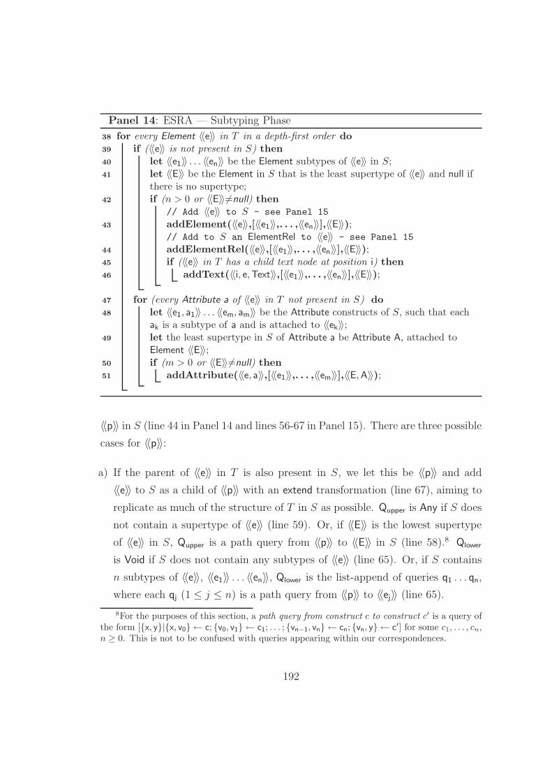
Panel 14: ESRA — Subtyping Phase
for every Element 〈〈e〉〉 in T in a depth-first order do38
if (〈〈e〉〉 is not present in S) then39
let 〈〈e1〉〉 . . . 〈〈en〉〉 be the Element subtypes of 〈〈e〉〉 in S;40
let 〈〈E〉〉 be the Element in S that is the least supertype of 〈〈e〉〉 and null if41
there is no supertype;if (n > 0 or 〈〈E〉〉6=null) then42
// Add 〈〈e〉〉 to S - see Panel 15
addElement(〈〈e〉〉,[〈〈e1〉〉,. . . ,〈〈en〉〉],〈〈E〉〉);43
// Add to S an ElementRel to 〈〈e〉〉 - see Panel 15
addElementRel(〈〈e〉〉,[〈〈e1〉〉,. . . ,〈〈en〉〉],〈〈E〉〉);44
if (〈〈e〉〉 in T has a child text node at position i) then45
addText(〈〈i, e,Text〉〉,[〈〈e1〉〉,. . . ,〈〈en〉〉],〈〈E〉〉);46
for (every Attribute a of 〈〈e〉〉 in T not present in S) do47
let 〈〈e1, a1〉〉 . . . 〈〈em, am〉〉 be the Attribute constructs of S, such that each48
ak is a subtype of a and is attached to 〈〈ek〉〉;let the least supertype in S of Attribute a be Attribute A, attached to49
Element 〈〈E〉〉;if (m > 0 or 〈〈E〉〉6=null) then50
addAttribute(〈〈e, a〉〉,[〈〈e1〉〉,. . . ,〈〈em〉〉],〈〈E,A〉〉);51
〈〈p〉〉 in S (line 44 in Panel 14 and lines 56-67 in Panel 15). There are three possible
cases for 〈〈p〉〉:
a) If the parent of 〈〈e〉〉 in T is also present in S, we let this be 〈〈p〉〉 and add
〈〈e〉〉 to S as a child of 〈〈p〉〉 with an extend transformation (line 67), aiming to
replicate as much of the structure of T in S as possible. Qupper is Any if S does
not contain a supertype of 〈〈e〉〉 (line 59). Or, if 〈〈E〉〉 is the lowest supertype
of 〈〈e〉〉 in S, Qupper is a path query from 〈〈p〉〉 to 〈〈E〉〉 in S (line 58).8 Qlower
is Void if S does not contain any subtypes of 〈〈e〉〉 (line 65). Or, if S contains
n subtypes of 〈〈e〉〉, 〈〈e1〉〉 . . . 〈〈en〉〉, Qlower is the list-append of queries q1 . . . qn,
where each qj (1 ≤ j ≤ n) is a path query from 〈〈p〉〉 to 〈〈ej〉〉 (line 65).
8For the purposes of this section, a path query from construct c to construct c′ is a query ofthe form [{x, y}|{x, v0} ← c; {v0, v1} ← c1; . . . ; {vn−1, vn} ← cn; {vn, y} ← c′] for some c1, . . . , cn,n ≥ 0. This is not to be confused with queries appearing within our correspondences.
192

Panel 15: ESRA — Procedures for the Subtyping Phase
/* ****** Procedure addElement(〈〈e〉〉,[〈〈e1〉〉,...,〈〈en〉〉],〈〈E〉〉) ****** */
let Qlower = 〈〈e1〉〉+ + . . . + +〈〈en〉〉 or Void if n = 0;52
if (〈〈E〉〉6=null) then let Qupper = 〈〈E〉〉;53
else Qupper = Any;54
extend(〈〈e〉〉,Range Qlower Qupper);55
/* **** Procedure addElementRel(〈〈e〉〉,[〈〈e1〉〉,...,〈〈en〉〉],〈〈E〉〉) **** */
if (〈〈e〉〉 in T has a parent Element which is present in S) then56
let 〈〈p〉〉 be the Element in S with the same label as the parent of 〈〈e〉〉 in T ;57
if (〈〈E〉〉6=null) then let Qupper be the path query from 〈〈p〉〉 to 〈〈E〉〉;58
else let Qupper = Any;59
else60
if (〈〈E〉〉6=null) then let 〈〈p〉〉 be 〈〈E〉〉 and Qupper = [{x, x}|x← 〈〈E〉〉];61
else62
let 〈〈p〉〉 be the lowest common ancestor of 〈〈e1〉〉. . . 〈〈en〉〉 in S and63
Qupper = Any;
for (every 〈〈ej〉〉 in [〈〈e1〉〉,. . . ,〈〈en〉〉]) do let qj be the path query from 〈〈p〉〉 to64
〈〈ej〉〉;let Qlower be q1 + + . . . + +qn, or Void if n = 0;65
let i be the number of children of 〈〈p〉〉;66
extend(〈〈i + 1, p, e〉〉,Range Qlower Qupper);67
/* ***** Procedure addText(〈〈i, e,Text〉〉,[〈〈e1〉〉,...,〈〈en〉〉],〈〈E〉〉) ***** */
for (every 〈〈ej〉〉 in [〈〈e1〉〉,. . . ,〈〈en〉〉]) do68
if (〈〈ej〉〉 has a child text node) then let qj = 〈〈ej,Text〉〉;69
else let qj = Void;70
let Qlower be q1 + + . . . + +qn;71
if (〈〈E〉〉6=null and has a child text node) then let Qupper = 〈〈E,Text〉〉;72
else let Qupper = Any;73
extend(〈〈i, e,Text〉〉,Range Qlower Qupper);74
/* * Procedure addAttribute(〈〈e, a〉〉,[〈〈e1, a1〉〉,...〈〈em, am〉〉],〈〈E,A〉〉) * */
if (m > 0) then75
for (every 〈〈ek, ak〉〉 in [〈〈e1, a1〉〉,. . . 〈〈em, am〉〉]) do76
let qk be the path query from 〈〈e〉〉 to 〈〈ek, ak〉〉 in S;77
let Qlower be q1 + + . . . + +qm;78
else let Qlower be Void ;79
if (〈〈E,A〉〉6=null) then let Qupper be the path query from 〈〈e〉〉 to 〈〈E,A〉〉 in S;80
else let Qupper = Any;81
extend(〈〈e, a〉〉,Range Qlower Qupper);82
193

b) If S contains a supertype 〈〈E〉〉 of 〈〈e〉〉 in T and possibly also subtypes of 〈〈e〉〉,
we let 〈〈p〉〉 be 〈〈E〉〉 (line 61). Qlower is derived in the same way as in Case (a)
above. Qupper is [{x, x}|x← 〈〈E〉〉], since each instance of 〈〈e〉〉 in S must be an
instance of 〈〈E〉〉 (line 61).
c) If S does not contain a supertype of 〈〈e〉〉, then it must contain one or more
subtypes of 〈〈e〉〉. In this case, we set 〈〈p〉〉 to be the lowest common ancestor of
these subtypes in S (line 63). Qlower is derived in the same way as in Case (a)
above. Qupper in this case is always Any, since S does not contain a supertype
of 〈〈e〉〉 (line 63).
If T contains an ElementRel 〈〈i, e, Text〉〉 connecting the current Element being
examined, 〈〈e〉〉, to the 〈〈Text〉〉 construct, this ElementRel is also added to S with
an extend transformation (line 46 in Panel 14 and lines 68-74 in Panel 15). If
S contains n subtypes of 〈〈e〉〉, 〈〈e1〉〉 . . . 〈〈en〉〉, then Qlower is the list-append of
queries qj (1 ≤ j ≤ n), where qj is 〈〈ej, Text〉〉 if 〈〈ej〉〉 has a child text node and
Void otherwise (lines 68-71 in Panel 15). If the least supertype of 〈〈e〉〉 in S is 〈〈E〉〉
and it has a child text node, then Qupper is 〈〈E, Text〉〉. If S does not contain a
supertype of 〈〈e〉〉, or if that Element does not have a child text node, then Qupper
is Any (lines 72-73 in Panel 15).
After handling an Element 〈〈e〉〉 of T , we then consider each Attribute 〈〈e, a〉〉
of 〈〈e〉〉 in T . We use the additional data structures built during the Initialisation
Phase of the ESRA to identify if S contains any subtypes or supertypes of 〈〈e, a〉〉
(lines 48 and 49). If it does, then we use these subtypes and supertypes to add
〈〈e, a〉〉 to S (line 51 in Panel 14 and lines 75-82 in Panel 15). If 〈〈e, a〉〉 is not
present in S, we add it to S with an extend transformation (line 82 in Panel 15).
Qlower is formulated using any Attribute subtypes of a, a1. . . am, present in S. Each
such Attribute ak is attached to an Element 〈〈ek〉〉. In particular, Qlower is the list-
append of queries q1. . . qm, where each qk is a path query from 〈〈e〉〉 to 〈〈ek, ak〉〉,
projecting on 〈〈e〉〉 and ak (lines 76-78 in Panel 15). If no subtypes of a exist in
S, then Qlower is Void. Qupper is formulated using the lowest supertype of 〈〈e, a〉〉
present in S, Attribute A, attached to Element 〈〈E〉〉. Qupper is a path query from
194

〈〈e〉〉 to 〈〈E, A〉〉, projecting on 〈〈e〉〉 and A (lines 80-81 in Panel 15). If no supertype
of 〈〈e, a〉〉 exists in S, then Qupper is Any.
We note here that each transformation that adds an Element to S or T re-
sults in an update in the data structure SourceEl or TargetEl. Similarly, each
transformation that adds an Attribute to S or T results in an update in data
structure SourceAtt or TargetAtt. We also note that, after the end of the Sub-
typing Phase, the ESRA goes through the data structures SourceElementRel
and TargetElementRel (which are used by Phase I) and for those ElementRel
constructs of S and T that did not originally have a corresponding path in the
other schema, the ESRA checks schemas Ssub and Tsub output by the Subtyping
Phase and provides the corresponding path in the other schema, if such a path
exists, since Ssub and Tsub have additional paths compared to S and T .
Dropping the Previous Assumptions
Up to this point, we have assumed that an Element 〈〈e〉〉 in T may only have
Element subtypes or supertypes in S. We now drop this assumption and consider
the case where an Element 〈〈e〉〉 in T has one or more Attribute subtypes or super-
types in S. In the following, we discuss the adjustments that need to be made to
the earlier description.
• Main method (Panel 14)
An Element 〈〈e〉〉 in T may also have Attribute constructs as subtypes and
supertypes in S. We therefore adjust lines 40 and 41 to reflect this.
• Procedure addElement (Panel 15)
The lower-bound query Qlower is defined as the list-append of the subtype
Element constructs present in S (lines 52-55). If, more generally, one of the
subtypes is an Attribute aj, attached to Element 〈〈ej〉〉, then the query that
contributes to Qlower is [x|{x, y} ← 〈〈ej, aj〉〉].
If the lowest supertype in S of 〈〈e〉〉 in T is A, attached to Element 〈〈E〉〉, then
the upper-bound query Qupper is [x|{x, y} ← 〈〈E, A〉〉].
195

• Procedure addElementRel (Panel 15)
This procedure adds to S an ElementRel that makes 〈〈e〉〉 a child of another
Element 〈〈p〉〉 in S. We have discussed above the three different possibilities:
(a) if 〈〈e〉〉 in T has a parent Element with label ℓ and an Element with label ℓ
exists in S, then we consider this as 〈〈p〉〉; (b) if S contains a supertype 〈〈E〉〉 of
〈〈e〉〉 in T , then we consider 〈〈E〉〉 as 〈〈p〉〉; (c) if S does not contain a supertype
of 〈〈e〉〉 in T , then we consider 〈〈p〉〉 to be the lowest common ancestor of the
subtypes of 〈〈e〉〉 in T that are present in S.
Generalising Case (a), if 〈〈e〉〉 in T has a parent Element with label ℓ and an
Attribute with the label ℓ exists in S, then we consider 〈〈p〉〉 to be the owner
Element of that Attribute of S. Generalising Case (b), if S contains an Attribute
A which is a supertype of 〈〈e〉〉 in T , then we consider 〈〈p〉〉 to be the owner
Element of A. Case (c) does not require any generalisation.
The lower-bound query Qlower is defined as q1++. . .++qn, where each qj is a
path query from 〈〈p〉〉 to the jth subtype, 〈〈ej〉〉, of 〈〈e〉〉 in S (lines 64-65). If,
more generally, the jth subtype is an Attribute 〈〈ej, aj〉〉, then query qj is a path
query from 〈〈p〉〉 to 〈〈ej, aj〉〉.
The upper-bound query Qupper is either the constant Any, or a query that uses
an Element 〈〈E〉〉, where 〈〈E〉〉 in S is the lowest supertype of 〈〈e〉〉 in T (lines 58
and line 61). If, more generally, the lowest supertype is an Attribute A, then
we use the owner Element of A to define Qupper.
• Procedure addText (Panel 15)
The lower-bound query Qlower is defined as q1++. . .++qn, where each qj is
〈〈ej, Text〉〉 (〈〈ej〉〉 being the jth subtype in S of 〈〈e〉〉). If, more generally, one of
the subtypes is an Attribute aj, attached to an Element 〈〈ej〉〉, then qj is 〈〈ej, aj〉〉.
The upper-bound query Qupper is 〈〈E, A〉〉, where A is the Attribute in S that is
the lowest supertype of 〈〈e〉〉 in T , and 〈〈E〉〉 is its owner Element.
Up to this point, we have also assumed that an Attribute a in T may only
have Attribute subtypes and supertypes in S. We now drop this assumption and
196

consider the case where an Attribute a in T has one or more Element subtypes
and supertypes in S. In the following, we discuss the adjustments that need to
be made to the earlier description.
• Main method (Panel 14)
An Attribute 〈〈e, a〉〉 in T may also have Element constructs as subtypes and
supertypes in S. We therefore adjust lines 48 and 49 to reflect this.
• Procedure addAttribute (Panel 15)
In cases where an Attribute in T has one or more subtype or supertype Element
constructs in S, then these constructs are also used to define the extent of the
Attribute of T . We therefore modify the queries specified in this procedure to
cater for element-to-attribute transformations for such cases.
If a subtype in S of 〈〈e, a〉〉 in T is an Element 〈〈ek〉〉, and S also contains an
ElementRel 〈〈ek, Text〉〉, then query qk in line 78 is a path query from 〈〈e〉〉 to
〈〈ek, Text〉〉, projecting on 〈〈e〉〉 and 〈〈Text〉〉.
Similarly, if the lowest supertype in S of 〈〈e, a〉〉 in T is an Element 〈〈E〉〉 and S
also contains an ElementRel 〈〈E, Text〉〉, then Qupper in line 78 is a path query
from 〈〈e〉〉 to 〈〈E, Text〉〉, projecting on 〈〈e〉〉 and 〈〈Text〉〉.
6.5.3 Applying the Subtyping Phase
We now illustrate the Subtyping Phase with respect to our running example.
When applied to Sconf , the Subtyping Phase traverses Tconf and first detects
that Element 〈〈Staff〉〉 in Tconf has subtypes 〈〈AcademicStaff〉〉 and 〈〈AdminStaff〉〉
in Sconf . It therefore adds 〈〈Staff〉〉 and 〈〈3, School, Staff〉〉 to Sconf with transfor-
mations 81 and 82 below, since 〈〈School〉〉 is the lowest common ancestor of
〈〈AcademicStaff〉〉 and 〈〈AdminStaff〉〉 in Sconf .9 It then detects that Attribute
9The enumeration of transformations listed here does not start from number 1, since theyare preceded by the transformations of the schema conformance phase, which are listed inAppendix A.
197

〈〈Staff, Staff.name〉〉 in Tconf has Element subtypes 〈〈AcademicStaff.name〉〉 and
〈〈AdminStaff.name〉〉 in Sconf and adds 〈〈Staff, Staff.name〉〉 to Sconf with transfor-
mation 83 . Next, it detects that 〈〈Staff.office〉〉 in Tconf has subtypes 〈〈Academic
Staff.office〉〉 and 〈〈AdminStaff.office〉〉 in Sconf and adds 〈〈Staff.office〉〉 to Sconf with
transformations 84 and 85 . Also, ElementRel 〈〈Staff.office, Text〉〉 in Tconf is added
to Sconf with transformation 86 . The resulting schema Ssub is shown in Figure 6.5
(grey denotes constructs existing before the application of the Subtyping Phase,
black denotes constructs added by the Subtyping Phase).
81 extendEl(〈〈Staff〉〉,Range (〈〈AcademicStaff〉〉+ +〈〈AdminStaff〉〉) Any)
82 extendER(〈〈3,School,Staff〉〉,Range Q1 Any), where Q1 is
[{x, y}|{x, y} ← 〈〈1,School,AcademicStaff〉〉] + +
[{x, y}|{x, y} ← 〈〈2,School,AdminStaff〉〉]
83 extendAtt(〈〈Staff,Staff.name〉〉,Range Q2 Any), where Q2 is
[{x, z}|{x, y} ← 〈〈1,AcademicStaff,AcademicStaff.name〉〉;
{y, z} ← 〈〈1,AcademicStaff.name,Text〉〉] + +
[{x, z}|{x, y} ← 〈〈1,AdminStaff,AdminStaff.name〉〉;
{y, z} ← 〈〈1,AdminStaff.name,Text〉〉]
84 extendEl(〈〈Staff.office〉〉,Range (〈〈AcademicStaff.office〉〉+ +〈〈AdminStaff.office〉〉) Any)
85 extendER(〈〈1,Staff,Staff.office〉〉,Range Q3 Any), where Q3 is
[{x, y}|{x, y} ← 〈〈1,AcademicStaff,AcademicStaff.office〉〉] + +
[{x, y}|{x, y} ← 〈〈1,AdminStaff,AdminStaff.office〉〉]
86 extendER(〈〈1,Staff.office,Text〉〉,Range Q4 Any), where Q4 is
〈〈1,AcademicStaff.office,Text〉〉+ +〈〈1,AdminStaff.officeText〉〉
When applied to Tconf , the Subtyping Phase traverses Sconf and detects that
Element 〈〈AcademicStaff〉〉 in Sconf has supertype 〈〈Staff〉〉 in Tconf and therefore
adds 〈〈AcademicStaff〉〉 and 〈〈2, Staff, AcademicStaff〉〉 to Tconf with transforma-
tions 87 and 88 below. It then detects that 〈〈AcademicStaff.name〉〉 in Sconf has
supertype 〈〈Staff, Staff.name〉〉 in Tconf and adds 〈〈AcademicStaff.name〉〉 in Tconf
with transformations 89 and 90 . ElementRel 〈〈1, AcademicStaff.name, Text〉〉 is
also added to Tconf with transformation 91 . Transformations 92 - 94 add Ele-
ment 〈〈AcademicStaff.office〉〉 and its associated ElementRel constructs to Tconf in
198

a way similar to Element 〈〈AcademicStaff.name〉〉. The rest of the transforma-
tions, 95 -102, are similar to transformations 87 - 94 , but now relate to Element
constructs 〈〈AdminStaff〉〉, 〈〈AdminStaff.name〉〉 and 〈〈AdminStaff.office〉〉. The re-
sulting schema Tsub is shown in Figure 6.6.
87 extendEl(〈〈AcademicStaff〉〉,Range Void 〈〈Staff〉〉)
88 extendER(〈〈2,Staff,AcademicStaff〉〉,Range Void [{x, x}|x← 〈〈Staff〉〉])
89 extendEl(〈〈AcademicStaff.name〉〉,Range Void [x|{x, y} ← 〈〈Staff,Staff.name〉〉])
90 extendER(〈〈2,AcademicStaff,AcademicStaff.name〉〉,
Range Void [{x, x}|x← 〈〈Staff,Staff.name〉〉])
91 extendER(〈〈1,AcademicStaff.name,Text〉〉,Range Void 〈〈Staff,Staff.name〉〉)
92 extendEl(〈〈AcademicStaff.office〉〉,Range Void 〈〈Staff.office〉〉)
93 extendER(〈〈2,AcademicStaff,AcademicStaff.office〉〉,
Range Void [{x, x}|x← 〈〈Staff.office〉〉])
94 extendER(〈〈1,AcademicStaff.office,Text〉〉,Range Void 〈〈1,Staff,Staff.office〉〉)
95 extendEl(〈〈AdminStaff〉〉,Range Void 〈〈Staff〉〉)
96 extendER(〈〈2,Staff,AdminStaff〉〉,Range Void [{x, x}|x← 〈〈Staff〉〉])
97 extendEl(〈〈AdminStaff.name〉〉,Range Void [x|{x, y} ← 〈〈Staff,Staff.name〉〉])
98 extendER(〈〈2,AdminStaff,AdminStaff.name〉〉,Range Void [{x, x}|x← 〈〈Staff〉〉])
99 extendER(〈〈1,AdminStaff.name,Text〉〉,Range Void 〈〈Staff,Staff.name〉〉)
100 extendEl(〈〈AdminStaff.office〉〉,Range Void 〈〈Staff.office〉〉)
101 extendER(〈〈2,AdminStaff,AdminStaff.office〉〉,Range Void [{x, x}|x← 〈〈Staff.office〉〉])
102 extendER(〈〈1,AdminStaff.office,Text〉〉,Range Void 〈〈1,Staff,Staff.office〉〉)
6.5.4 Applying Phase I and Phase II
After the application of the Subtyping Phase to the source and target schemas,
the ESRA applies Phase I and Phase II to the schemas output by the Subtyping
Phase. As discussed earlier, Phase I and Phase II of the ESRA are identical to
those of the SRA, and we refer the reader to Chapter 5 for their description. We
note, however, that the schemas that are input to Phase I are the schemas that
are output by the application of the Subtyping Phase to S and T , not S and T .
Referring to our running example, the application of the Phase I to schemas
199

Ssub
University.belongs.College.belongs.School.belongs.
AcademicStaff
2University.belongs.College.belongs.
School.belongs.
AcademicStaff.
name
1
Text
1 1
University.belongs.College.belongs.
School.belongs.
AcademicStaff.
office
University.belongs.College.belongs.School.belongs.
AdminStaff
2University.belongs.College.belongs.
School.belongs.
AdminStaff.
name
1University.belongs.College.belongs.
School.belongs.
AdminStaff.
office
1 2
11
University
University.belongs.College.
belongs.School
1
University.belongs.College.belongs.
School.belongs.Staff
University.belongs.College.belongs.School.
belongs.Staff.name
3
1
University.belongs.College.belongs.
School.belongs.Staff.office
1
Figure 6.5: Schema Ssub, Output of the Subtyping Phase for Schema Sconf .
Tsub
University.belongs.College.belongs.
School.belongs.Staff
Text
University.belongs.College.belongs.
School.belongs.Staff.office1
1
2
University.belongs.College.belongs.School.
belongs.Staff.name
University.belongs.College.belongs.School.belongs.
AdminStaff
University.belongs.College.belongs.
School.belongs.
AcademicStaff.
name
University.belongs.College.belongs.
School.belongs.
AcademicStaff.
office
University.belongs.College.belongs.
School.belongs.
AdminStaff.
name
University.belongs.College.belongs.
School.belongs.
AdminStaff.
office
21
University.belongs.College.belongs.School.belongs.
AcademicStaff
21
1111
2 3
University.belongs.
College.nameUniversity.belongs.
College
Figure 6.6: Schema Tsub, Output of the Subtyping Phase for Schema Tconf .
Ssub and Tsub has no effect on either schema. The application of Phase II to
schema Ssub results in the transformation pathway listed below:
200

103 extendEl(〈〈College〉〉,Range Void Any)
104 extendER(〈〈1,Staff.office,College〉〉,Range Void Any)
105 extendAtt(〈〈College,College.name〉〉,Range Void Any)
106 addER(〈〈1,Staff,AcademicStaff〉〉,
[{y, z}|{x, y} ← 〈〈3,School,Staff〉〉; {x, z} ← 〈〈1,School,AcademicStaff〉〉])
107 addER(〈〈2,Staff,AdminStaff〉〉,
[{y, z}|{x, y} ← 〈〈3,School,Staff〉〉; {x, z} ← 〈〈1,School,AdminStaff〉〉])
The resulting schema, Sres, is illustrated in Figure 6.8 (grey denotes constructs
existing before the application of Phase II, black denotes constructs added by the
Phase II).
The application of Phase II to schema Tsub results in the transformation path-
way listed below:
108 extendEl(〈〈University〉〉,Range Void Any)
109 extendEl(〈〈School〉〉,Range Void Any)
110 extendER(〈〈3,School,Staff〉〉,Range Void Any)
111 extendER(〈〈1,School,AcademicStaff〉〉,Range Void Any)
112 extendER(〈〈2,School,AdminStaff〉〉,Range Void Any)
The resulting schema, Tres, is illustrated in Figure 6.9. We see that schemas
Sres and Tres are identical, and this is asserted by injecting (automatically) a
series of id transformations between them.
Figure 6.7 illustrates the overall transformations in our running example after
the application of the ESRA. Numbers in white circles denote transformations
produced by the ESRA, while numbers in dark circles denote their reverse trans-
formations.
Sdata source
idSres Tres
datasource
1 56
1 56
Tconf TSsubSconf Tsub
81 86
81 86
102 87
102 87
80 57
80 57
112 108
112 108
103 107
103 107
Figure 6.7: Running Example after Application of the ESRA.
201

Sres
University.belongs.College.belongs.School.belongs.
AcademicStaff
2University.belongs.College.belongs.
School.belongs.
AcademicStaff.
name
1
Text
1 1
University.belongs.College.belongs.
School.belongs.
AcademicStaff.
office
University.belongs.College.belongs.School.belongs.
AdminStaff
2University.belongs.College.belongs.
School.belongs.
AdminStaff.
name
1University.belongs.College.belongs.
School.belongs.
AdminStaff.
office
1 2
11
University
University.belongs.College.
belongs.School
1
University.belongs.College.belongs.
School.belongs.Staff
University.belongs.College.belongs.School.
belongs.Staff.name
3
1
University.belongs.College.belongs.
School.belongs.Staff.office
1
1
1
University.belongs.
College.nameUniversity.belongs.
College
2
Figure 6.8: Schema Sres.
Tres
University.belongs.College.belongs.
School.belongs.Staff
Text
University.belongs.College.belongs.
School.belongs.Staff.office1
1
2
University.belongs.College.belongs.School.
belongs.Staff.name
University.belongs.College.belongs.School.belongs.
AdminStaff
University.belongs.College.belongs.
School.belongs.
AcademicStaff.
name
University.belongs.College.belongs.
School.belongs.
AcademicStaff.
office
University.belongs.College.belongs.
School.belongs.
AdminStaff.
name
University.belongs.College.belongs.
School.belongs.
AdminStaff.
office
21
University.belongs.College.belongs.School.belongs.
AcademicStaff
21
1111
2 3
University.belongs.
College.nameUniversity.belongs.
College
University
University.belongs.College.
belongs.School
1
1 2
3
Figure 6.9: Schema Tres.
202

6.5.5 Discussion
The ESRA is able to use subtyping information between schema constructs of
the source and target schemas in order to produce a transformation pathway
that avoids the possible loss of information that would have occurred if the SRA
of Chapter 5 had been used. For example, it is clear from Figure 6.4 (which shows
the conformed schemas input to the ESRA in our running example) that using
the SRA instead of the ESRA would have resulted in a transformation pathway
that would not transform any data from the data source of S to the data source
of T .
We also observe that the ESRA is not tightly coupled with our ontology-based
schema conformance technique. For example, subtyping information between
schema constructs of the source and target schemas could be specified manually by
the user, or could be semi-automatically produced by a schema matching tool, e.g.
by deriving subsumption relationships as discussed in [Riz04]. This demonstrates
the independence of the schema conformance and schema transformation phases
of our overall approach to XML data transformation/integration.
Finally, by performing a complexity analysis similar to that of the SRA in
Chapter 5, it is straightforward to conclude that the complexity of the Subtyping
Phase is O(ES hT ) + O(ET hS), where ES and ET are the number of Element
constructs of S and T , and where hS and hT are the heights of S and T . Therefore,
the overall complexity of the ESRA is the same as that of the SRA, i.e.:
O(ES + ET ) + O(AS + AT ) + O(ES hT ) + O(ET hS)
6.6 Summary
This chapter has made two key contributions. First, we have presented an
ontology-based schema conformance technique. Compared to the schema match-
ing technique presented in Chapter 5, this technique is more scalable in a peer-
to-peer setting where all peers need to exchange data with all other peers, since it
allows schemas to be conformed individually with respect to an ontology, rather
203

than pairwise with each other. Second, we have extended the schema restructur-
ing algorithm of Chapter 5 with the ability to use subtyping information when
generating the transformation pathway between the source and target schemas.
In a setting where the constructs of the source and target schemas have subtype
and/or supertype relationships between them, our extended schema restructuring
algorithm is able to avoid the loss of information that would have occurred if the
algorithm of Chapter 5 had been used.
Our schema conformance technique uses correspondences from XML schemas
to one or more ontologies as a way of providing semantics for these schemas. When
correspondences are (manually or semi-automatically) defined from multiple XML
schemas to one ontology, then the correspondences are used to automatically
conform these XML schemas to the ontology. When correspondences are defined
from multiple XML schemas to multiple ontologies, and assuming that these
ontologies are linked via AutoMed transformation pathways, it is still possible to
conform the XML schemas to a single ontology. Our approach therefore promotes
correspondence reusability by allowing the use of multiple ontologies.
Apart from [BL04], which was developed in parallel with our approach, our
ontology-based schema conformance technique is the only other technique that
employs ontologies for schema conformance. Compared to [BL04], our approach
provides richer correspondences using 1-n, n-1 and schema-to-data GLAV rules
while still preserving the same degree of automation. Moreover, our approach
demonstrates the use of multiple ontologies as a ‘semantic bridge’, which is only
briefly discussed in [BL04]. Regarding schema transformation, our extended
schema restructuring algorithm maintains the ability to avoid loss of information
caused by structural incompatibility between the source and target schemas, by
generating a synthetic extent for those target schema constructs that are absent
from the source schema.
204

Chapter 7
Transformation and Integration
of Real-World Data
7.1 Overview
Chapter 5 presented in detail our approach for XML data transformation and
integration, provided a complexity analysis of the schema restructuring algorithm,
and discussed the correctness of this algorithm (which is covered in more detail
in Appendix B). Chapter 6 then extended our approach with the ability to
use ontologies for schema conformance, and subtyping information for schema
transformation.
We now investigate the application of our approach in four case studies, illus-
trating centralised, service-oriented and peer-to-peer data transformation/integra-
tion scenarios. Each case study examines a particular real-world application set-
ting and demonstrates one or more aspects of our approach.
In particular, Section 7.2 describes the application of our approach to the in-
tegration of heterogeneous relational biological data sources. The aim of this case
study is to demonstrate (a) the applicability of our approach for the integration of
non-XML data sources, and (b) the benefit of using our approach to separate the
manual/semi-automatic schema conformance phase from the automatic schema
transformation phase. Section 7.3 describes the application of our approach for
205

the transformation of crime data that has been exported in XML format from a
relational database, demonstrating schema transformation and aiming to assess
schema materialisation using our approach. Section 7.4 describes the applica-
tion of our approach to the semantic reconciliation of services whose input and
output formats correspond to the same ontology, and aiming to demonstrate:
(a) an application setting where the scalability of our ontology-based schema
conformance technique is a significant factor, (b) real-world correspondences to
ontologies handled by our ontology-based schema conformance technique, and (c)
the applicability of our approach for service composition, thereby providing a uni-
form approach to workflow and data integration. Section 7.5 describes a similar
application setting that aims to demonstrate the applicability of our ontology-
based schema conformance technique in a setting where services correspond to
different ontologies that have been integrated using AutoMed.
Performance timings for the schema restructuring algorithm are given in the
first two case studies, and for all the automatic algorithms in the second case
study. These are not the result of rigorous performance evaluations, and should
be considered only as indicative of the performance of our algorithms. Also, as
is discussed at the end of these two case studies, there is significant scope for
improvement in terms of the performance of the AutoMed repository and the
query processor.
The case studies described in this chapter are representative examples of the
particular problems they address, and have been chosen after consulting with
experts in each specific domain. We note, however, that care must be taken
not to over-generalise the conclusions of each case study. In particular, the first
case study is representative of using our approach for integrating relational data
sources. However, the data source schemas in the case study are small (less than
10 tables), and so additional experimentation is required to investigate the per-
formance of our approach before applying it to larger data sources, e.g. whose
schemas contain hundreds of tables. The second case study is representative of
XML data transformation and materialisation using our approach. Again, addi-
tional experimentation is required for evaluating the performance implications for
206

materialising larger data sources. The third case study is representative of service
reconciliation in bioinformatics, and of our ontology-based schema conformance
technique; it is not, however, representative of XML schema transformation in
general, as the service inputs and outputs are very simple. The fourth case study
is representative of our ontology-based schema conformance technique in a set-
ting with multiple ontologies, but is again not representative of XML schema
transformation in general, since service inputs and outputs are very simple.
7.2 Integration of Heterogeneous Data Sources
Using an XML Layer
This section presents an architecture for integrating heterogeneous biological data
sources, and reports on our experiences in using this architecture to provide an
integrated resource that supports analysis, mining and visualisation of functional
genomics1 data. This architecture was developed as part of the BioMap2 project.
The data integration framework used for this application setting, described in
Section 7.2.1, was developed by other colleagues and is presented in more detail
in [MZR+05]. Our own contribution, namely the use of our approach as a unifying
XML ‘layer’ for the integration of heterogeneous data sources, is described in
Sections 7.2.2 and 7.2.3.
7.2.1 The BioMap Setting
Biological data sources are highly heterogeneous in terms of their data model,
schemas, nomenclature and data formats [DOB95]. Such data sources also fre-
quently make use of large numbers of unstable, inconsistent identifiers for biolog-
ical entities [Cla03]. The architecture described in this section handles these two
1Functional genomics [HB97] is a field of molecular biology focusing on the gene functionsand interactions, often based on the large scale analyses of the genomic data or the entiregenomes.
2See http://www.biochem.ucl.ac.uk/bsm/biomap
207

Cluster Data
Cluster Data
Data Source
Data Source
AutoMed toolkit
Global Database
AutoMed Metadata
Repository
Global Schema
Schema Schema Schema Schema
Figure 7.1: Architectural Overview of the Data Integration Framework
issues by combining two data integration techniques, the first for addressing data
heterogeneity and the second for resolving the issue of inconsistent identifiers.
BioMap is a collaborative project involving UCL, Birkbeck, Brunel, EBI3 and
ICH4, aiming to develop a data warehouse that integrates a variety of experi-
mental biological data. The aim of BioMap is to provide an integrated resource
that supports analysis, mining and visualisation of functional genomics data. The
BioMap data warehouse is implemented within Oracle, extending techniques de-
veloped for the CATH-PFDB database [SMJ+02] and is designed to serve as a
source for further data marts5 which could themselves be constructed using the
AutoMed-based techniques presented here. Current data sources to the BioMap
data warehouse include CATH [OMJ+97], KEGG [KGK+04], Gene3D [LGMO04],
Gene Ontology [ABB+00], MSD [GOT+04] and ten other specialist resources.
The BioMap data integration architecture is illustrated in Figure 7.1. There
are two principal sources of information for the global database (i.e. the BioMap
data warehouse) — data sources and cluster data.
Each data source is an externally maintained resource that is to be integrated
3European Bioinformatics Institute, http://www.ebi.ac.uk4Institute of Child Health, http://www.ich.ucl.ac.uk/ich5A data mart is a database derived from one or more data warehouses that contains a
portion of the data contained in the warehouses, often in a summarised form.
208

as part of the global database. A data source could be a conventional relational
or other structured database, or a semi-structured data source, such as an XML
file. Conceptually, a data source describes facts about biological entities. We
listed above some of the major data sources of the BioMap project.
Each cluster data resource is constructed from one or more data sources and
provides the basis for a generally applicable approach to the integration of data
lacking a common reference identifier. Conceptually, a cluster data resource pro-
vides a data-dependent classification of the entities within data sources into re-
lated sets (see [MZR+05]).
Wrappers provided by the AutoMed Toolkit automatically generate the Au-
toMed internal representations of the Schemas and the Global Schema shown in
Figure 7.1, and store these in the AutoMed Metadata Repository. The AutoMed
toolkit and our own schema restructuring algorithm are then used to generate the
transformation pathways from the Schemas to the Global Schema. These path-
ways can be used for (virtual) query processing over the source schemas, and for
materialising and incrementally maintaining the data warehouse — see [MZR+05]
and [FP03] for details.
7.2.2 The Integration Process
The integration process consists of the following steps:
1. Automatic generation of the AutoMed relational schemas, LS1, . . . , LSn,
corresponding to the Data Source and Cluster Data Schemas.
2. Similarly, automatic generation of the AutoMed relational schema, GS, cor-
responding to the Global Schema, i.e. the schema of the Global Database.
3. Automatic translation of schemas LS1, . . . , LSn and GS into the corre-
sponding XMLDSS schemas X1, . . . , Xn and GX.
4. Conformance of each schema Xi to GX by means of appropriate rename
transformations, to ensure that only semantically equivalent schema con-
structs share the same name, and that all equivalent schema constructs do
209

share the same name. This results in a set of new schemas X ′
1, . . . , X′
n.
5. Application of any necessary data cleansing transformations on each X ′
i,
creating a set of schemas X ′′
1 , . . . , X ′′
n.
6. Restructuring of each schema X ′′
i to GX by applying our schema restruc-
turing algorithm to each pair of schemas X ′′
i and GX.
The above integration process results in n transformation pathways, LSi →
Xi → X ′
i → X ′′
i → GX → GS, from the schema of each data source or cluster
data resource to the global schema, where the pathway GX → GS is common
for all n pathways.
Steps 1 and 2 are carried out automatically by AutoMed’s relational wrapper,
as discussed in Chapter 3. Steps 3 to 6 are explained in more detail below.
Step 3: Translating AutoMed relational to XMLDSS schemas. To
translate a relational schema to an XMLDSS schema we first generate a graph,
G, from the relational schema. G contains a node for each table in the relational
schema and also contains an edge from the node corresponding to table R1 to
the node corresponding to table R2 if there is a foreign key in R2 referencing the
primary key of R1. In the given relational schemas there are no cycles in G — in
a general setting, we would have to break any cycles at this point. We then create
a set of trees, T , obtained by traversing G from each node that has no incoming
edges, and we convert T into a single tree by adding a generic root. We finally
use T to generate the pathway from the relational schema to its corresponding
XMLDSS schema, as described in Panel 16.
To illustrate the translation, the top of Figure 7.2 illustrates a part of the
schema of the CLUSTER data source (where foreign keys have the same name
as the primary keys they reference). At the bottom of the figure, the XMLDSS
schema that corresponds to this relational schema is illustrated. Similarly, Fig-
ure 7.3 illustrates a part of the relational global schema and the corresponding
AutoMed XMLDSS schema.
Step 4: Schema Conformance. Our schema restructuring algorithm, used
in Step 5 of the integration process, assumes that if two schema constructs in
210

Panel 16: XMLDSS Schema Generation from Relational Schema using TreeStructure T
Input: Tree structure TOutput: XMLDSS schema Xi
for (each node t in a depth-first traversal of T ) do83
if (t is the root) then84
Insert the Text construct into Xi.85
Insert the root itself as an Element construct.86
else87
Insert t as an Element.88
Insert an ElementRel construct from the parent of t to t.89
Find the columns ci belonging to the table that corresponds to t.90
for (each ci) do91
Insert ci as an Element construct.92
Insert an ElementRel construct from t to ci.93
Insert an ElementRel construct from ci to Text.94
Remove the now redundant relational constructs from Xi.95
the source and in the target schema, respectively, have the same name, then they
refer to the same real-world concept, and if they do not have the same name,
they do not. Thus, after the XMLDSS schemas are produced, and before the
application of the schema restructuring algorithm in Step 5, a number of rename
transformations are manually issued on each source XMLDSS schema by a domain
expert (this process could also have been performed semi-automatically using a
schema matching tool together with our PathGen tool, as discussed in Chapter 5).
In our running example, the domain expert produced the following rename
transformations on the XMLDSS schema in Figure 7.2:113 rename(〈〈CLUSTER$1〉〉,〈〈GLOBAL$1〉〉)
114 rename(〈〈DESCRIPTION$1〉〉,〈〈ASSIGNMENT DESCRIPTION$1〉〉)
115 rename(〈〈SEQUENCE SOURCE ID$1〉〉,〈〈PSEQID$1〉〉)
116 rename(〈〈SEQUENCE SOURCE ID$2〉〉,〈〈SEQUENCE SOURCE ID$1〉〉)
117 rename(〈〈SEQUENCE SOURCE ID$3〉〉,〈〈SSEQID$1〉〉)
118 rename(〈〈SEQUENCE SOURCE ID$4〉〉,〈〈SEQUENCE SOURCE ID$2〉〉)
119 rename(〈〈ASSIGNMENT TYPE ID$2〉〉,〈〈PASSID$1〉〉)
120 rename(〈〈ASSIGNMENT TYPE ID$3〉〉,〈〈ASSIGNMENT TYPE ID$2〉〉)
211

ASSIGNMENT_TYPES
PK ASSIGNMENT_TYPE_ID
DESCRIPTION
CLUSTER_DATA
PK CLUSTER_ID
FK1 ASSIGNMENT_TYPE_IDFK2 SEQUENCE_SOURCE_ID
SEQUENCES
PK SEQUENCE_ID
FK1 SEQUENCE_SOURCE_ID
SEQUENCE_SOURCES
PK SEQUENCE_SOURCE_ID
CLUSTER_DATA$1
SEQUENCE_SOURCES$1
2
PCData
SEQUENCES$1
3
CLUSTER$1
2
CLUSTER_DATA$2
ASSIGNMENT_TYPES$1
1
13
ASSIGNMENT_TYPE_ID$2
DESCRIPTION$1
2
1
1 SEQUENCE_SOURCE_ID$4
CLUSTER_ID$2
ASSIGNMENT_TYPE_ID$3
SEQUENCE_SOURCE_ID$3
SEQUENCE_ID$1
2
3 1
1 1
1
1
1
2
1
SEQUENCE_SOURCE_ID$2
CLUSTER_ID$1
ASSIGNMENT_TYPE_ID$1
1
1 1
1
2
SEQUENCE_SOURCE_ID$1
1
3
1
Figure 7.2: Top: part of the CLUSTER relational schema. Bottom: correspond-ing part of the CLUSTER XMLDSS schema.
and the following rename transformation on the XMLDSS schema in Figure 7.3:
121 rename(〈〈SEQUENCE SOURCE ID$2〉〉,〈〈SSEQID〉〉)
Step 5: Data cleansing. After the local XMLDSS schemas have been
conformed with the global XMLDSS schema, the domain expert can manually is-
sue any further necessary transformations to remove any representational hetero-
geneities at the data level. For example, consider in our running example attribute
212

CLUSTER_DATA
PK CLUSTER_ID
ASSIGNMENT_TYPE_ID ASSIGNMENT_DESCRIPTION SEQUENCE_SOURCE_ID
SEQUENCES
PK SEQUENCE_ID
SEQUENCE_SOURCE_ID
PCData
GLOBAL$1
CLUSTER_DATA$1
ASSIGNMENT_ DESCRIPTION$1
CLUSTER_ID$1
1
1
ASSIGNMENT_ TYPE_ID$1
SEQUENCE_ SOURCE_ID$1
4 2
1
1 1
3
SEQUENCES$1
SEQUENCE_ SOURCE_ID$2
SEQUENCE_ID$1
1
2 1
1 1
2
Figure 7.3: Left: Part of the Global Relational Schema. Right: CorrespondingPart of the XMLDSS Schema.
DESCRIPTION in relation ASSIGNMENT TYPES which is called DESCRIPTION$1
in the CLUSTER XMLDSS schema (see Figure 7.2). The extent of this attribute
in the data source consists of mixed case strings, whereas in the global schema
these Text instances are expected to be uppercase strings. To turn these to upper-
case strings, the transformations below can be appended to the transformation
pathway resulting from the conformance step (i.e. Step 4 above). Here upperCase
is a built-in IQL function that converts all the alphabetic characters in a string
to uppercase.
122 add(〈〈0,ASSIGNMENT DESCRIPTION$1,Text〉〉,
[{v0, upperCase v1}|{v0, v1} ← 〈〈1,ASSIGNMENT DESCRIPTION$1,Text〉〉])
123 contract(〈〈1,ASSIGNMENT DESCRIPTION$1,Text〉〉,[])
124 rename(〈〈0,ASSIGNMENT DESCRIPTION$1,Text〉〉,
〈〈1,ASSIGNMENT DESCRIPTION$1,Text〉〉)
Step 6: Automatic restructuring of each data source schema X ′′
i
into the global XMLDSS schema GX. In this particular setting, our schema
restructuring algorithm is not supplied with any subtyping information. Transfor-
mations 125-134, given below, transform the 〈〈SEQUENCE SOURCES$1〉〉 subtree
213

of the schema arising from the CLUSTER XMLDSS schema (Figure 7.2) after
the data cleansing step into the partial global XMLDSS schema (Figure 7.3). The
transformations that add to the global XMLDSS schema GX the subtree with
Element 〈〈ASSIGNMENT TYPES$1〉〉 as its root are similar to transformations 129-
134, i.e. the empty list is the query supplied to all the transformations.
// Application of schema restructuring algorithm on source XMLDSS schema
// (in this case, the XMLDSS schema derived from the CLUSTER data source)
125 add(〈〈1,GLOBAL$1,CLUSTER DATA$1〉〉,
[{v0, v2}|{v0, v1} ← 〈〈1,GLOBAL$1,SEQUENCE SOURCES$1〉〉;
{v1, v2} ← 〈〈2,SEQUENCE SOURCES$1,CLUSTER DATA$1〉〉])
126 extend(〈〈3,CLUSTER DATA$1,ASSIGNMENT DESCRIPTION$1〉〉,
[{v1, v2}|{v0, v1} ← 〈〈3,ASSIGNMENT TYPES$1,CLUSTER DATA$2〉〉;
{v0, v2} ← 〈〈2,ASSIGNMENT TYPES$1,DESCRIPTION$1〉〉])
127 rename(〈〈3,CLUSTER DATA$1,SEQUENCE SOURCE ID$1〉〉,
〈〈4,CLUSTER DATA$1,SEQUENCE SOURCE ID$1〉〉)
128 add(〈〈2,GLOBAL$1,SEQUENCES$1〉〉,
[{v0, v2}|{v0, v1} ← 〈〈1,GLOBAL$1,SEQUENCE SOURCES$1〉〉;
{v1, v2} ← 〈〈3,SEQUENCE SOURCES$1,SEQUENCES$1〉〉])
// Application of schema restructuring algorithm on target XMLDSS schema
// (in this case, the global XMLDSS schema GX)
129 add(〈〈SEQUENCE SOURCES$1〉〉,[])
130 add(〈〈1,GLOBAL$1,SEQUENCE SOURCES$1〉〉,[])
131 add(〈〈1,SEQUENCE SOURCES$1,SEQUENCE SOURCE ID$1〉〉,[])
132 add(〈〈1,SEQUENCE SOURCE ID$1,Text〉〉,[])
133 add(〈〈2,SEQUENCE SOURCES$1,CLUSTER DATA$1〉〉,[])
134 add(〈〈3,SEQUENCE SOURCES$1,SEQUENCES$1〉〉,[])
...
214

7.2.3 Implementation and Results
The data integration process described above was carried out on a Pentium 4
2.8Ghz, with 1Gb RAM and Linux as the operating system. The Gene3D,
KEGG Gene, KEGG Genome, KEGG Orthology, CATH and CLUSTER data
sources, and the global database are all Oracle databases, while the AutoMed
Repository is a PostgreSQL database. Note that the Linux machine that per-
formed the integration was located on a different site than that hosting the
databases, and this had a negative impact on the performance of the integra-
tion process.
Each of the involved data source schemas contained up to 5 tables, while the
global schema contained 25 tables. Each of the transformation pathways used
to integrate the data source schemas with the global schema contained between
800 and 1000 transformations. The run-time of the integration process, i.e. Steps
1–6 described above — including the manually created transformations of Steps
4 and 5, took under 15 minutes for each data source, resulting in a total running
time of about 85 minutes. This time compares favourably with the likely time
it would take to manually specify and populate view definitions for the global
schema in terms of the data source schemas.
Note that the experiment was performed in late 2004 using an early version
of our schema restructuring algorithm described in Chapter 5 that lacked a num-
ber of significant performance optimisations. One of these optimisations was to
derive the correct order number for ElementRel constructs at the time of their
insertion, rather than inserting each one with an order of -1 and then reordering
all ElementRel constructs after all other insert/delete operations. As a result, the
current schema restructuring algorithm would have produced pathways ranging
from 400 to 600 transformations, resulting in a lower running time.
215

7.3 XML Data Transformation and Materialisa-
tion
This section presents the application of our schema restructuring and materiali-
sation algorithms for the transformation of crime data from a source XML rep-
resentation to a target XML representation, and the subsequent materialisation
of the latter using data associated with the former.
Section 7.3.1 first describes the crime data transformation and materialisation
setting and Section 7.3.2 discusses the extraction of XML DataSource Schemas
in this setting. Sections 7.3.3, 7.3.4 and 7.3.5 discuss schema conformance, re-
structuring and materialisation in this setting.
7.3.1 The Crime Informatics Setting
Police forces in the U.K. maintain burglary-related crime data in relational databases
that do not necessarily share the same schema, and, as a result, collaboration
across police forces incurs a significant overhead. To address this problem, an
XML interchange format has been developed by the Crime Informatics group at
Birkbeck, and our XML schema and data transformation approach can be used
to materialise this XML format using data from each police force. This section
discusses the application of our approach to data from a single police force —
more general application would be similar.
Figure 7.4 illustrates the crime data transformation setting for a single police
force. Each force is responsible for exporting its relational data in XML format,
e.g. using relational-to-XML converters built into their DBMS of choice. This
XML document is then semi-automatically conformed to use the same termi-
nology as the target XML format (transformation pathway XS ↔ XSconf) and
then our schema restructuring algorithm is responsible for providing the pathway
between the conformed source schema and the target schema (transformation
pathway XSconf ↔ XT ).
216

XS XSconf
RDBMS
idXSres XTres XT
XMLfile
XMLfile
Figure 7.4: The Crime Data Transformation and Materialisation Setting.
7.3.2 XMLDSS Schema Extraction
The crime data stored in the relational database of the particular police force con-
sists of a single table with 211 columns. From these, about 65 store information
such as date, time and location, whereas the rest represent boolean statements
about the crime, such as whether the burglar exited through the front door or
whether the burglar stole any jewelry. As a result of this design, the table is quite
sparse. Furthermore, since the database consists of a single table with multiple
attributes, the exported XML document is shallow, as illustrated below, and so
the XMLDSS schema corresponding to this XML document (generated using the
DOM XMLDSS extraction algorithm of Chapter 4) is similarly shallow, as shown
in Figure 7.5.
<document>
<row>
<ID>23</ID>
<CRIME_REF>961615</CRIME_REF>
<DATE_COMMITTED>02-MAR-00</DATE_COMMITTED>
...
<jewel>1</jewel>
<keys>0</keys>
<bags>0</bags>
...
</row>
...
</document>
217

row
ID CRIME_REF DATE_COMMITTED jewel
document
Text
... ... ... keys bags
Figure 7.5: The XMLDSS Schema for the Exported XML Document.
Note that the exported XML document contains carriage returns and inden-
tations between element tags which make the XML document more readable.
However, if we were to extract an XMLDSS schema from the XML document
as it is, this ‘whitespace’ text would result in an invalid XMLDSS schema, since
XMLDSS does not support mixed content elements (as discussed in Chapter 4).
For this reason, we chose to enable the WHITESPACE COLLAPSE6 option of the
XMLWrapperFactory when creating the source and target XMLWrapper objects
(XMLWrapperFactory options were discussed in Chapter 4).
The target schema is shown in Figure 7.6. To create it, the crime domain
experts produced a sample XML document containing instances of all possible
information that is desirable to appear in the target, and then its corresponding
XMLDSS schema was automatically generated, again using the DOM XMLDSS
extraction algorithm of Chapter 4 with the WHITESPACE COLLAPSE option enabled.
Compared to the source schema, the target schema is not as shallow. Further-
more, many of the source schema boolean fields are modelled as lists of values
in the target XMLDSS schema, and the source XMLDSS schema contains 626
constructs whereas the target XMLDSS schema contains only 57. For example,
the target schema construct mo keywords (modus operandi keywords) contains all
6The semantics of the WHITESPACE COLLAPSE option are identical to those of XML Schema,i.e. the whitespace prefix and suffix of a text node is removed, and if this results in an emptystring, then the text node is deleted.
218

crm28
id circumstances scene_of_crime goods_taken
root
Text
modus_operandi crime_scene_ officer_report
address property_type
when_committed
from to portability
description value
mo_ description
point_of_ entry
method_ used
item mo_
keywords
Figure 7.6: The Target XMLDSS Schema.
keywords relating to the characteristics of the burglary (points of entry and exit,
whether the alarm was disabled etc.), whereas these are represented as more than
100 boolean-valued elements in the source schema, one element per keyword.
7.3.3 Schema Conformance
After generating the source and target XMLDSS schemas, XS and XT , we pro-
ceed to the schema conformance phase, which will create pathway XS ↔ XSconf
in Figure 7.4. The schema conformance phase in this example is performed man-
ually after consultation with the crime domain experts, and transforms schema
XS into schema XSconf (see Figure 7.4), which uses the same terminology and
describes information at the same level of granularity as schema XT .
Table 7.1 gives the transformations of pathway XS → XSconf . Query q1
concatenates the text of elements 〈〈LOCN NUMBER$1〉〉, 〈〈LOCN STREET$1〉〉,
〈〈LOCN DISTRICT$1〉〉, 〈〈LOCN TOWN$1〉〉 and 〈〈LOCN POSTCODE$1〉〉, using
commas as a separator. Similarly, queries q2 and q3 concatenate the text of
elements 〈〈TIME FIRST COMMITTED$1〉〉, 〈〈DATE FIRST COMMITTED$1〉〉 and
〈〈TIME LAST COMMITTED$1〉〉, 〈〈DATE LAST COMMITTED$1〉〉, respectively.
219

Table 7.1: Transformation pathway XS → XSconf .135 rename(〈〈document$1〉〉,〈〈root$1〉〉) 136 rename(〈〈row$1〉〉,〈〈crm28$1〉〉)137 rename(〈〈ID$1〉〉,〈〈id$1〉〉) 138 rename(〈〈MO NOTES$1〉〉,〈〈circumstances$1〉〉)139 add(〈〈address$1〉〉,q1) 140 rename(〈〈LOCATION DESC$1〉〉,〈〈property type$1〉〉)141 add(〈〈from$1〉〉,q2) 142 add(〈〈to$1〉〉,q3)143 add(〈〈item$1〉〉,q4) 144 add(〈〈item$1, category〉〉,q6)145 add(〈〈goods taken$1〉〉,q7) 146 add(〈〈crm28$1, goods taken$1〉〉,q8)147 add(〈〈goods taken$1, item$1〉〉,q5) 148 add(〈〈mo keywords$1〉〉,q9)149 add(〈〈crm28$1,mo keywords$1〉〉,q10) 150 add(〈〈mo keywords$1,Text〉〉,q11)151 rename(〈〈MO DESC$1〉〉,〈〈mo description$1〉〉)
Transformations 143-144 perform an n-1 element-to-attribute transformation.
The source schema contains many elements with a domain of 0/1 that correspond
to items stolen during the burglary, e.g. whether the burglars stole jewelry, cash
and so on. In the target schema, there exists one instance of element 〈〈item$1〉〉
for each stolen item. Query q4 therefore generates as many instances for element
〈〈item$1〉〉 as there are columns with a value of 1 for a specific burglary, while
queries q5 and q6 create the necessary instances for ElementRel 〈〈crm28$1, item$1〉〉
and Attribute 〈〈item$1, category〉〉, respectively. Note that the attribute takes val-
ues from the labels of the respective elements of the export XML document. After
generating the extents for element 〈〈item$1〉〉, element 〈〈goods taken〉〉 is created,
together with the necessary 〈〈crm28$1, goods taken$1〉〉 ElementRel construct (the
cardinality for this is 1-1). Note that ElementRel 〈〈goods taken$1, item$1〉〉 will be
created by the schema restructuring algorithm.
Similarly, transformations 148-150 perform an n-1 element-to-element transfor-
mation. The source schema contains many elements with a domain of 0/1 that
correspond to the modus operandi of the burglary, whereas the target schema
contains a single element, 〈〈mo keywords〉〉, that contains a list of modus operandi
keywords that correspond to the labels of the source schema elements.
7.3.4 Schema Restructuring
After creating schema XSconf , we can now apply the schema restructuring algo-
rithm to create pathway XSconf ↔ XT . The algorithm restructures both schema
220

XSconf , creating schema XSres, and schema XT , creating schema XTres, render-
ing them identical and then applies an id transformation between the two (see
Figure 7.4). Pathway XSconf ↔ XSres consists of 60 transformations, pathway
XT ↔ XTres consists of 618 transformations, and including the id transformation
between schemas XSres and XTres, the overall pathway XSconf ↔ XT consists
of 679 transformations.
We tested the running times for the XMLDSS schema extraction algorithm,
the schema conformance and the schema restructuring algorithm using an export
XML document containing approximately 100 rows (586Kb). The time required
to create the source and target XMLDSS schemas was about 50 seconds, the
time consumed by the schema conformance phase was about 35 seconds, and the
time taken by the schema restructuring algorithm was 90 seconds. Most of the
running time, i.e. over 90%, is spent by the AutoMed repository, not the actual
algorithms.
7.3.5 Schema Materialisation
After creating the transformation pathway XS ↔ XT , we are now able to mate-
rialise XMLDSS schema XT with data from the data source of XMLDSS schema
XS. For this purpose, we use our XMLDSS schema materialisation algorithm,
described in Chapter 4, which uses the DOM API.
We successfully applied our XMLDSS schema materialisation algorithm, dis-
cussed in Chapter 4, to the file mentioned above. The export XML document
was materialised in 36 minutes. The very poor performance is attributable to
a number of causes: to the queries supplied with the transformations of the
schema conformance phase, involving the 150 boolean-valued elements (transfor-
mations 143-150); to the AutoMed query processor; and to the use of the DOM
API for this setting. In particular, the current AutoMed query processor does
not support the efficient evaluation of the join operator and path queries are per-
formed using a nested-loops join algorithm for each step. The use of the DOM
221

API means that only single schemes can be handled by the AutoMed XML wrap-
per and the entire burden of evaluating path queries falls to the AutoMed query
processor. If the eXist native XML database had been used, then these path
queries would have been delegated to eXist’s query engine for evaluation, and the
materialisation of schema XT would have been much faster.
7.4 Service Reconciliation Using A Single On-
tology
This section presents an approach for the reconciliation of bioinformatics services
using our schema and data transformation approach together with a scientific
workflow tool. This work was developed as part of the ISPIDER project7.
Section 7.4.1 introduces the problem of bioinformatics service reconciliation
and Section 7.4.2 reviews current approaches related to service interoperability.
Section 7.4.3 introduces our proposed approach for a scalable solution to the
problem of bioinformatics service reconciliation and Section 7.4.4 applies this ap-
proach to a particular case study, for the reconciliation of services that correspond
to the same ontology.
7.4.1 Bioinformatics Service Reconciliation
In recent years, the bioinformatics field has seen an explosion in the number of
services offered to the community. These platform-independent software compo-
nents have consequently been used for the development of complex tasks through
service composition within workflows, thereby promoting reusability of services.
However, the large number of services available impedes service composition and
so developing techniques for semantic service discovery that would significantly
reduce the search space is of great importance [LAWG05].
After discovering services that are relevant to one’s interests, the next step
is to identify whether these services are functionally compatible. Bioinformatics
7See http://www.ispider.manchester.ac.uk
222

services are independently created by many parties worldwide, using different
technologies and data types, hindering integration and reusability [Ste02]. As a
result, after discovering two such services, the researcher needs to identify whether
the output of the first is compatible with the input of the second (based on a num-
ber of factors, such as the technology employed by each service, the representation
format and the data type used), and then provide a means of reconciliation, if
the services are not functionally compatible.
In practice, compatible services are rare. Within the Taverna8 workflow tool,
service technology reconciliation is addressed by using Freefluo [OAF+04], an
extensible workflow enactment environment that bridges the gap between web
services and other service types, such as web-based REST9 services. However,
the researcher still needs to reconcile the outputs and inputs of services in terms
of content, data type and representation format, spending time and effort in de-
veloping functionality that, even though essential for the services to interoperate,
is irrelevant to the experiment.
The primary cause of this problem is the existence of multiple different data
types and representation formats even for basic concepts, such as DNA sequences.
Most current service composition tools concentrate on a specific data type and
representation format (or combinations of pairs of types and formats, when
translation is needed) to accomplish a highly specific task, rather than being
generic [LBW+04]. As a result, reusability of existing tools is low.
Another common practice in bioinformatics is the use of flat-file representation
formats for the overwhelming majority of data types, while the adoption rate
of XML is low. This practice does not allow the application of Semantic Web
technologies and solutions to their full extent, such as semantically annotating
different pieces of information within a bioinformatics data type.
We argue that (a) the use of XML and (b) allowing the annotation and ma-
nipulation of service inputs and outputs at a fine-grained level, can boost service
8See http://taverna.sourceforge.net9Representational State Transfer (REST): stateless services that support caching.
223

interoperability in a scalable manner. It is important that the amount of anno-
tations required be kept to a minimum, given that service providers are usually
disinclined to provide comprehensive annotations for their services. We have de-
veloped an approach for the reconciliation of services by exploiting the (manual)
semantic annotation of service inputs and outputs to one ontology (discussed
in this section), or several interconnected ontologies (discussed in Section 7.5),
and the subsequent automatic restructuring of the XML output of one service
to the required XML input of another using our schema restructuring algorithm.
Although our approach uses XML as the common representation format, non-
XML services are also supported by the use of converters to and from XML. Our
approach can be used for service reconciliation in two different ways: either me-
diating between services as a service itself, e.g. from within a workflow tool, or
statically by generating mediating services.
7.4.2 Related Work in Service Reconciliation
Research such as [SK03, MBE03, BDSN02] has mainly focused on service tech-
nology composition, matchmaking and routing, assuming that service inputs and
outputs are a priori compatible. This assumption is restrictive, as it is often the
case that two services are semantically compatible, but cannot interoperate due
to data type and/or representation format mismatches.
This problem has forced service consumers to handle such mismatches with
custom code from within the calling services. In an effort to minimise this issue
and promote service reusability, myGrid10 has fostered the notion of shims [HSL+04],
i.e. services that act as intermediaries between services and reconcile their inputs
and outputs. However, a new shim needs to be manually created for each pair
of services that need to interoperate. [HSL05] states that, even though in theory
the number of shims that myGrid needs to provide is quadratic in the number of
services it contains, the actual number of shims should be much smaller. How-
ever, this manual approach is not scalable, as in 2005 myGrid gave access to 1,000
10See http://www.mygrid.org.uk
224

services [LAWG05], while in 2007 this number was over 3,000.
[BL04] describes a scalable framework that uses mappings to one or more on-
tologies, possibly containing subtyping information, for reconciling the output of
a service with the input of another. The sample implementation of this frame-
work is able to use mappings to a single ontology in order to generate an XQuery
query as the transformation program.
We observe that [BL04] only provides for shim generation, whereas our ap-
proach provides a uniform approach to workflow and data integration, both of
which are key aspects of in silico biological experiments. Furthermore, our ap-
proach differs from [BL04] in a number of aspects and provides a more generic
solution to the problem of bioinformatics service reconciliation. First, we also
consider services that produce or consume non-XML data and also allow primi-
tive data type reconciliation, whereas [BL04] does not. Moreover, we allow 1-n
GLAV correspondences, compared to the 1-1 LAV correspondences of [BL04] and
we also define a methodology for reconciling services that correspond to more
than one ontology (discussed in Section 7.5). We also note that our XML schema
restructuring algorithm is able to avoid loss of information during data transfor-
mation, by analysing the hierarchical nature of the source and target schemas
and by using subtype information provided by the ontologies.
[TAK05] also uses a mediator system for service composition. However, the
focus is either to provide a service over the global schema of the mediator, whose
data sources are services, or to generate a new service that acts as an interface over
other services. In contrast, we reconcile a sequence of semantically compatible
services that need to form a pipeline: there is no need for a single ‘global schema’
or a single new service to be created.
7.4.3 Our Service Reconciliation Approach
Consider a service S1 that produces data that need to be consumed by another
service S2. Our service reconciliation consists of the following 4 steps, illustrated
in Figure 7.7:
225

Step 1: XML as the common representation format. We handle differ-
ences in the representation format by using XML as the common representation
format. If the output/input of a service is not in XML, then a format converter
is needed to convert to/from XML.
Step 2: XMLDSS as the schema type. We use our own XMLDSS schema
type for the XML documents input to and output by services. We recall that
an XMLDSS schema can be automatically generated from an XML document or
from an accompanying DTD/XML Schema if this is available.
Step 3: Correspondences to typed ontologies. We use one or more on-
tologies as a ‘semantic bridge’ between services. Providers or users of services
semantically annotate the inputs and outputs of services by defining correspon-
dences between an XMLDSS schema and an ontology. Ontologies are assumed
to be typed, i.e. each concept is associated with a data type, and so defining
correspondences resolves both the semantic heterogeneity and the data type het-
erogeneity encountered between schemas (a discussion on the different types of
heterogeneity was given in Chapter 2).
Steps 4-5: Schema and data transformation. We use the schema con-
formance and the schema restructuring algorithms described in Chapter 6 to
automatically transform the XMLDSS schema of S1 to the XMLDSS schema of
S2.
If service S1 does not have an accompanying DTD or XML Schema for its
output, sample XML output documents for S1 must be provided, and these must
represent all valid formats that S1 is able to produce, so as to create an XMLDSS
schema that represents all possible instances of the output of S1. If this is not
possible, then an XMLDSS can be extracted at run-time for every new instance
XML document output by S1. The same applies for the input of S2.
Our approach for service reconciliation can support two different architectures:
Shim generation: With this approach, we use the AutoMed system and our
226

XMLDSSschema X1
S1 output XML format
S2 input XML format
(2) (2)
(5) (3) (3)
C1 C2
XMLDSSschema X’1
XMLDSSschema X’2
(4) (4)
XMLDSSschema X2
S1 output non-XML
format
S2 input non-XML
format
(1) (1)
Service S2
Service S1
Step 1: format translation to and from XMLStep 2: automatic XMLDSS schema generationStep 3: manual correspondences definitionStep 4: automatic XMLDSS schema conformanceStep 5: automatic XMLDSS schema restructuring
Ontology O1
Figure 7.7: Reconciliation of services S1 and S2 using ontology O1.
schema transformation approach to generate shims, i.e. tools or services for the
reconciliation of services, by generating transformation scripts which are then
incorporated within the workflow tool.
Mediation service: With this architecture, the workflow tool invokes service
S1, receives its output, and submits this output and a handle on service S2 to
a service provided by the AutoMed system. This service uses our approach to
transform the output of S1 to a suitable input for consumption by S2.
With the shim generation approach, AutoMed is not part of the run-time
architecture, and so it is necessary to export AutoMed’s mediation functionality.
This functionality consists of the format converters, the algorithms for generating
an XMLDSS schema from an XML document, a DTD or an XML Schema, and
our schema transformation algorithms.
Format converters are not a part of the AutoMed toolkit and so can be used
227

from within a workflow tool, without exporting any AutoMed functionality. The
converters can be either incorporated within the workflow tool, or their function-
ality can be imported using services. As an example, a number of shims in myGrid
are format converters.
The XMLDSS schema type does not require AutoMed functionality, and so
the XMLDSS schema derivation algorithms can be used from within a workflow
tool in the same way as format converters.
The XMLDSS schema conformance and schema restructuring algorithms de-
scribed in Chapter 6 are currently tightly coupled with the AutoMed system. To
use our approach without integrating AutoMed with a workflow tool, we need to
export this functionality. To this effect, Chapter 4 has presented an algorithm
that derives a single XQuery query Q, able to materialise X2 using data from X1,
using the transformation pathway X1 → X ′
1 → X ′
2 → X2 produced by the two
algorithms.
We now discuss a case study that demonstrates the mediation service ap-
proach.
7.4.4 Case Study Using A Single Ontology
Figure 7.8 illustrates a sample workflow with three services that will be used to
demonstrate our approach. Listings of all service inputs, outputs and XMLDSS,
XML Schema and DTD schemas discussed in this section are given in Appendix C.
getIPIEntry getPfamEntry getInterProEntry
UniProt
entry (flat file
format)
Pfam
entry (flat file
format)
IPI
accession (string)
Pfam
accession (string)
T 2
InterPro
entry (XML file
format)
T 1
InterPro
accession (string)
Figure 7.8: Sample Workflow.
The first service takes as input an IPI11 accession number, e.g. IPI00015171,
and outputs the corresponding IPI entry as a flat file using the UniProt12 format.
11International Protein Index, see http://www.ebi.ac.uk/IPI.12Universal Protein Resource, see http://www.ebi.uniprot.org.
228

The second service receives an InterPro13 accession number and returns the cor-
responding InterPro entry. The third service receives a Pfam14 accession number
and returns the corresponding Pfam entry. In this workflow, two transformations
are needed: T1 extracts the InterPro accession number from an IPI entry that
uses the UniProt format, while T2 extracts the Pfam accession number from an
InterPro entry.
We now apply the mediation service approach for the reconciliation of the
services of the workflow of Figure 7.8.
Step 1: XML as a common representation format. Service getIPIEntry
outputs a flat file that follows the UniProt representation format15 and contains
a single entry consisting of multiple lines. Each line consists of two parts, the
first being a two-character line code, indicating the type of data contained in the
line, while the second contains the actual data, consisting of multiple fields.
Since UniProt also has an XML representation format specified by an XML
Schema16, we created a format converter that, given an IPI flat file f that follows
the UniProt format, converts f to an XML file conforming to that XML Schema.
Service getInterProEntry outputs an XML file and so there is no need for
a format converter. Concerning the input of the second and the third service,
they each take as input a single string, representing an InterPro/Pfam accession
number, respectively. The input XML documents for these contain a single XML
element, ip acc and pf acc, respectively, with a PCData node as a single child,
as shown below. For these, the format converters implement the functionality of
the XPath expressions /ip acc/text() and /pf acc/text(), respectively.
<ip_acc>InterPro_accession_string</ip_acc>
<pf_acc>Pfam_accession_string</pf_acc>
Step 2: XMLDSS schema generation. As discussed above, service getIPIEntry
13See http://www.ebi.ac.uk/interpro.14See http://www.sanger.ac.uk/Software/Pfam.15IPI also supports the FASTA representation format, containing less information.16Available at http://www.pir.uniprot.org/support/docs/uniprot.xsd
229

outputs a flat file which is converted to an XML file that conforms to the UniProt
XML Schema. An XMLDSS schema for the output of this service is automat-
ically derived from that XML Schema. Similarly, an XMLDSS schema for the
output of service getInterProEntry is automatically derived using the InterPro
DTD schema17.
Concerning the input of the second and the third service, the corresponding
XMLDSS schemas are automatically extracted by using a single sample XML
document for each, such as the ones given earlier.
Step 3: Correspondences. After generating the required XMLDSS schemas
for our workflow, we need to specify the correspondences between these schemas
and an ontology. In this example, we have used the typed myGrid OWL domain
ontology18.
As discussed in Chapter 6, it is not necessary to provide a complete set of
correspondences between an XMLDSS schema and an ontology, if the XMLDSS
constructs that are not mapped to the ontology are not needed for the trans-
formation. This property is particularly significant in this setting in terms of
applicability and scalability, as it allows for incrementally defining the full set of
correspondences between an XMLDSS schema and an ontology: one can define
only those correspondences relevant to the specific problem at hand, instead of
the full set of correspondences.
In our example, this means that we only need to specify correspondences
for those constructs of the XMLDSS schema of the output of getIPIEntry
that contribute to the input of service getInterProEntry. Consequently, we
need to specify correspondences for only two constructs, 〈〈dbReference$9〉〉 and
〈〈dbReference$9, id〉〉 (see Table 7.2). The first models an entry in a bioinformatics
data resource, whose type is specified by 〈〈dbReference$9, type〉〉. The type of a
resource is modelled in IPI using data values, whereas in the ontology it is mod-
elled as classes, and so n correspondences are required for this construct, where
17Available at ftp://ftp.ebi.ac.uk/pub/databases/interpro/interpro.dtd18Available at http://www.mygrid.org.uk/ontology.
230

Table 7.2: Correspondences between the XMLDSS schema of the output ofgetIPIEntry and the myGrid ontology.
Construct: 〈〈dbReference$9〉〉Extent: [{d}|{d, t} ← 〈〈dbReference$9, type〉〉; t =′ InterPro′]
Path: 〈〈InterPro record〉〉
Construct: 〈〈dbReference$9〉〉Extent: [{d}|{d, t} ← 〈〈dbReference$9, type〉〉; t =′ Pfam′]
Path: 〈〈Pfam record〉〉
Construct: 〈〈dbReference$9, id〉〉Extent: [{d, i}|{d, i} ← 〈〈dbReference$9, id〉〉;
{d, t} ← 〈〈dbReference$9, type〉〉; t =′ InterPro′]Path: [{ir, l}|{ia, ir} ← 〈〈part of, InterPro accession, InterPro record〉〉;
{ia, l} ← 〈〈datatype, InterPro accession,Literal〉〉]
Construct: 〈〈dbReference$9, id〉〉Extent: [{d, i}|{d, i} ← 〈〈dbReference$9, id〉〉;
{d, t} ← 〈〈dbReference$9, type〉〉; t =′ Pfam′]Path: [{pr, l}|{pa, pr} ← 〈〈part of,Pfam accession,Pfam record〉〉;
{pa, l} ← 〈〈datatype,Pfam accession,Literal〉〉]
n is the number of types of resources that IPI supports and that also exist in
the ontology. Each of these correspondences maps 〈〈dbReference$9〉〉 to a class in
the ontology representing a bioinformatics data resource record and specifies the
part of the extent of 〈〈dbReference$9〉〉 to which the correspondence applies. For
example, the first correspondence states that those instances of 〈〈dbReference$9〉〉
whose 〈〈dbReference$9, type〉〉 Attribute has a data value of ‘InterPro’, map to
the 〈〈InterPro record〉〉 ontology class. For simplicity, but without loss of generality,
we only provide the two correspondences related to InterPro and Pfam.
The XMLDSS schema of the input of service getInterProEntry consists of a
single Element construct, 〈〈ip acc〉〉, which corresponds to class 〈〈InterPro accession〉〉
in the ontology, and of an ElementRel construct, 〈〈1, ip acc, Text〉〉. The correspon-
dences are given in Table 7.3. The correspondences for the XMLDSS schema of
the input of the third service, getPfamEntry, are not listed as they are similar.
231
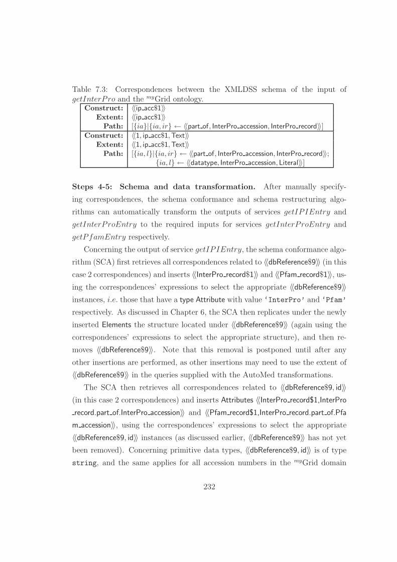
Table 7.3: Correspondences between the XMLDSS schema of the input ofgetInterPro and the myGrid ontology.
Construct: 〈〈ip acc$1〉〉Extent: 〈〈ip acc$1〉〉
Path: [{ia}|{ia, ir} ← 〈〈part of, InterPro accession, InterPro record〉〉]
Construct: 〈〈1, ip acc$1,Text〉〉Extent: 〈〈1, ip acc$1,Text〉〉
Path: [{ia, l}|{ia, ir} ← 〈〈part of, InterPro accession, InterPro record〉〉;{ia, l} ← 〈〈datatype, InterPro accession,Literal〉〉]
Steps 4-5: Schema and data transformation. After manually specify-
ing correspondences, the schema conformance and schema restructuring algo-
rithms can automatically transform the outputs of services getIPIEntry and
getInterProEntry to the required inputs for services getInterProEntry and
getPfamEntry respectively.
Concerning the output of service getIPIEntry, the schema conformance algo-
rithm (SCA) first retrieves all correspondences related to 〈〈dbReference$9〉〉 (in this
case 2 correspondences) and inserts 〈〈InterPro record$1〉〉 and 〈〈Pfam record$1〉〉, us-
ing the correspondences’ expressions to select the appropriate 〈〈dbReference$9〉〉
instances, i.e. those that have a type Attribute with value ‘InterPro’ and ‘Pfam’
respectively. As discussed in Chapter 6, the SCA then replicates under the newly
inserted Elements the structure located under 〈〈dbReference$9〉〉 (again using the
correspondences’ expressions to select the appropriate structure), and then re-
moves 〈〈dbReference$9〉〉. Note that this removal is postponed until after any
other insertions are performed, as other insertions may need to use the extent of
〈〈dbReference$9〉〉 in the queries supplied with the AutoMed transformations.
The SCA then retrieves all correspondences related to 〈〈dbReference$9, id〉〉
(in this case 2 correspondences) and inserts Attributes 〈〈InterPro record$1,InterPro
record.part of.InterPro accession〉〉 and 〈〈Pfam record$1,InterPro record.part of.Pfa
m accession〉〉, using the correspondences’ expressions to select the appropriate
〈〈dbReference$9, id〉〉 instances (as discussed earlier, 〈〈dbReference$9〉〉 has not yet
been removed). Concerning primitive data types, 〈〈dbReference$9, id〉〉 is of type
string, and the same applies for all accession numbers in the myGrid domain
232

ontology, so there is no need for any type-casting operations.
Concerning the input of getInterProEntry, the SCA uses the first corre-
spondence to rename 〈〈ip acc$1〉〉 to 〈〈InterPro record.part of.InterPro accession$1〉〉,
while the second correspondence, which is a primitive data type reconciliation
correspondence, is of no consequence as both the input of the service and the
ontology model InterPro accession numbers use the string data type.
After the application of the SCA, the XMLDSS schema X2 of the input of
service getInterProEntry contains three constructs, 〈〈InterPro record.part of.Int
erPro accession$1〉〉, 〈〈Text〉〉 and an ElementRel linking these two constructs. The
XMLDSS schema of the output of service getIPIEntry, X1, contains a number of
constructs, but the only ones relevant to those of X2 are 〈〈InterPro record$1〉〉 and
〈〈InterPro record$1,InterPro record.part of.InterPro accession〉〉. The schema restruc-
turing algorithm (SRA) therefore applies a number of contract transformations
supplied with the queries Void and Any, so as to remove non-relevant constructs.
The only non-trivial transformation is the attribute-to-element transformation:
first Element 〈〈InterPro record.part of.InterPro accession$1〉〉 is added to X1 using
the extent of Attribute 〈〈InterPro record$1,InterPro record.part of.Inter Pro accession〉〉,
then ElementRel 〈〈InterPro record.part of.InterPro accession$1,Text〉〉 is added, again
using the Attribute extent, and finally the Attribute is deleted.
After applying the SRA, we finally employ the XMLDSS schema materiali-
sation algorithm to materialise X2, i.e. the input of service getInterProEntry,
using data from the data source of X1, i.e. the output of service getIPIEntry,
using the transformation pathway X1 → X ′
1 → X ′
2 → X2.
The application of Steps 4 and 5 for the second part of the workflow in Fig-
ure 7.8 is similar.
233

7.5 Service Reconciliation Using Multiple On-
tologies
This section describes the application of our schema and data transformation
approach for the reconciliation of service-based e-learning systems, i.e. systems
whose functionality is exposed via services. In general, the services of each system
may correspond to a different ontology, each of which is linked to a single learning
domain ontology via a BAV transformation pathway. This work was developed
for the MyPlan19 project.
Section 7.5.1 introduces our example setting in which two e-learning systems,
each using a different ontology, need to exchange data. Section 7.5.2 presents the
transformation of each e-learning ontology into the domain e-learning ontology,
forming the semantic bridge between the two e-learning systems — a role that
was assumed by a single ontology in the previous case study. Next, Section 7.5.3
describes the use of the semantic bridge in order to conform the inputs and
outputs of services of the two systems and Section 7.5.4 describes the subsequent
schema and data transformation process.
7.5.1 e-Learning Service Reconciliation
The MyPlan project aims to develop models of learners and to support them in
planning their lifelong learning. One goal of MyPlan is to facilitate interoperabil-
ity in a scalable fashion between existing systems targeted at the lifelong learner.
Since direct access to these systems’ repositories is in general not possible, an
approach based on reconciling and combining the services these systems provide
is being explored.
For our running example here, suppose we need to transfer learners’ data from
the L4All20 system to the eProfile21 system. Each system is accompanied by an
ontology. L4All uses the L4ALL RDFS ontology, developed specifically for the
19See http://www.lkl.ac.uk/research/myplan20See http://www.lkl.ac.uk/research/l4all21See http://www.schools.bedfordshire.gov.uk/im/EProfile
234

L4All system, while eProfile uses the Friend-Of-A-Friend OWL-DL ontology22
(FOAF is OWL-Full, but we only use its OWL-DL subset here). A Lifelong
Learning Ontology, LLO (defined in OWL-DL), developed as part of the MyPlan
project, aims to encompass all concepts relating to lifelong learners [BMP08].
Figure 7.9 illustrates a portion of each of these three ontologies.
Suppose now we need to transform the output of a service S1 which retrieves
data about a learner from L4All, to become the input of a service S2 which inserts
data about that learner into eProfile. Listed below are a sample output from S1:
<user>
<userID>John</userID>
<fullname>John Smith</fullname>
<age>1970</age> <gender>F</gender>
<email>[email protected]</email>
<travel>15</travel> <location>London</location>
<occupation>Technology Professional</occupation>
<qual><![CDATA[PhD]]></qual>
<skills><![CDATA[write good reports]]></skills>
<interests><![CDATA[Sport]]></interests>
</user>
and a sample input for S2:
<eProfile>
<accountName>Mike2008</accountName>
<mbox>[email protected]</mbox>
<name>Mike Jonson</name>
<interest>sport</interest>
</eProfile>
Compared to the setting of Section 7.4, our approach in this multiple ontolo-
gies setting contains one more step, which is the formation of the transformation
pathways between the two system ontologies, L4ALL and FOAF, and the domain
ontology, LLO, but does not require Step 2, as the services in this setting produce
and consume XML files (see Figure 7.10). These services may or may not have
22See http://www.foaf-project.org
235

X 2 eProfile$1
mbox$1
2
accountName$1
1
PCData
1 1
interest$1
name$1
3
4
1 1
X 1 user$1
fullname$1
userID$1
1
PCData
1 1
... email$1
5
1
1
interests$1 ...
11 2
L4ALL
Learner rdfs:Literal
Identification
interests Learning _Prefs learning-prefs
username
id name
LLO
Learner rdfs:Literal
Identification
topicInterest Interest
hasInterest
userID has
Identification email
full Name
FOAF
rdfs:Literal
name
accountName
holdsAccount
mbox topic Interest
owl:Thing
Person Online
Account
Agent
Figure 7.9: Left: Ontologies L4ALL, LLO and FOAF. Right: XMLDSS schemasX1 and X2.
an accompanying DTD/XML Schema for their inputs and outputs, and so Step 3
either extracts an XMLDSS schema from the accompanying DTD/XML Schema,
or from sample input/output XML documents provided for the services, if such
a schema does not exist.
Similarly to the setting of Section 7.4, the result of this process is a transfor-
mation pathway X1 ↔ X ′
1 ↔ X ′
2 ↔ X2, which can then be used at run-time by
the MyPlan service broker to automatically generate data compliant with service
S2 from data output by service S1. We discuss Steps 1 and 3-6 in more detail
next, after briefly describing the transformation of each system’s ontology into
the domain ontology of our setting.
7.5.2 Transforming Ontologies using AutoMed
The transformation of the L4ALL and FOAF ontologies into the LLO ontology
using AutoMed requires the creation of transformation pathways L4ALL→LLO
236

XMLDSSschema X1
S1 output XML format
S2 input XML format
(3) (3)
(6)L4ALL FOAF
(4) (4)
LLO AutoMedpathway
AutoMedpathway
C1 C2C’1
XMLDSSschema X’1
XMLDSSschema X’2
(5) (5) (5)
XMLDSSschema X2
(1) (1)
S1 output non-XML
format
S2 input non-XML
format
(2) (2)
Service S2
Service S1
Step 1: ontology integrationStep 2: format translation to and from XMLStep 3: automatic XMLDSS schema generationStep 4: manual correspondences definitionStep 5: automatic XMLDSS schema conformanceStep 6: automatic XMLDSS schema restructuring
Figure 7.10: Reconciliation of Services S1 and S2.
and FOAF→LLO. L4ALL and LLO overlap significantly, but L4ALL is expressed
in RDFS while LLO is expressed in OWL-DL. Both FOAF and LLO are expressed
in OWL-DL, but FOAF is a general-purpose ontology while LLO targets lifelong
learning.
Overcoming the modelling language heterogeneity problem between L4ALL
and LLO is straightforward: each L4ALL RDFS construct is transformed into an
equivalent OWL construct. For example, to replace the RDFS class 〈〈l4 : Learner〉〉
with the equivalent OWL-DL class with the same name, the following transfor-
mations are applied to L4ALL:
add(〈〈llo : Learner〉〉,〈〈l4 : Learner〉〉)
delete(〈〈l4 : Learner〉〉,〈〈llo : Learner〉〉)
The first transformation above adds the OWL-DL construct 〈〈llo : Learner〉〉 to
L4ALL, specifying that its extent is equivalent to the extent of the RDFS con-
struct 〈〈l4 : Learner〉〉. The RDFS construct 〈〈l4 : Learner〉〉 can then be deleted,
specifying that its extent is equivalent to the extent of the OWL-DL construct
〈〈llo : Learner〉〉. Note that, since a number of properties reference the 〈〈l4 : Learner〉〉
237

Table 7.4: Fragment of the Transformation Pathway L4ALL→LLO.. . . add/extend steps for L4ALL→LLO. . .
152 delete(〈〈l4 : id, l4 : Learner, l4 : Identification〉〉,〈〈llo : hasIdentification, llo : Learner, llo : Identification〉〉)
153 delete(〈〈l4 : learning − prefs, l4 : Learner, l4 : Learning Prefs〉〉,〈〈llo : hasInterest, llo : Learner, llo : Interest〉〉)
154 delete(〈〈l4 : interests, l4 : Learning Prefs, rdfs : Literal〉〉,〈〈llo : topicInterest, llo : Interest, rdfs : Literal〉〉)
155 delete(〈〈l4 : Learner〉〉,〈〈llo : Learner〉〉)156 delete(〈〈l4 : email, l4 : Identification, rdfs : Literal〉〉,
〈〈llo : email, llo : Identification, rdfs : Literal〉〉)157 delete(〈〈l4 : username, l4 : Identification, rdfs : Literal〉〉,
〈〈llo : userID, llo : Identification, rdfs : Literal〉〉)158 delete(〈〈l4 : name, l4 : Identification, rdfs : Literal〉〉,
〈〈llo : fullName, llo : Identification, rdfs : Literal〉〉). . . more delete/contract steps for L4ALL→LLO. . .
class, in practice these would have to be deleted before deleting that class. Ta-
ble 7.4 lists a fragment of the delete steps within the pathway, as these steps will
be referred to again later in this section.
After translating the L4ALL ontology from RDFS to OWL-DL, the rest of
the pathway L4ALL↔LLO is formed by specifying transformations that address
the structural and semantic heterogeneities of the two ontologies (since the data
model heterogeneity has already been addressed). The result is the transforma-
tion of the L4ALL ontology into an ontology that is identical to LLO, and this is
asserted by automatically injecting a series of id transformations between them.
Regarding the integration of the FOAF and LLO ontologies, the transforma-
tion pathway FOAF→ LLO first adds to FOAF all the LLO constructs and then
deletes from FOAF all FOAF constructs. Table 7.5 lists a fragment of the delete
steps within the pathway LLO → FOAF, as these will be referred to again —
note that pathway LLO → FOAF is the reverse of the pathway FOAF → LLO.
We note from 166 that 〈〈llo : Learner〉〉 is equivalent to 〈〈foaf : Agent〉〉. Also, since
FOAF does not contain a class analogous to 〈〈llo : Interest〉〉 in the LLO, in 165 we
use an IQL function genClass to generate as many instances of class 〈〈llo : Interest〉〉
as there are instances of property 〈〈foaf : topic interest, foaf : Person, owl : Thing.〉〉.
238

Table 7.5: Fragment of the transformation pathway LLO→FOAF. . . add/extend steps for LLO→FOAF. . .
159 delete(〈〈llo : userID, llo : Identification, rdfs : Literal〉〉,[{ag, lit}|{ag, oa} ← 〈〈foaf : holdsAccount, foaf : Agent, foaf : OnlineAccount〉〉;
{oa, lit} ← 〈〈foaf : accountName, foaf : OnlineAccount, rdfs : Literal〉〉])160 delete(〈〈llo : fullName, llo : Identification, rdfs : Literal〉〉,
[{t, lit}|{t, lit} ← 〈〈foaf : name, owl : Thing, rdfs : Literal〉〉; member t 〈〈foaf : Agent〉〉])161 delete(〈〈llo : email, llo : Identification, rdfs : Literal〉〉,
[{y, z}|{x, y, z} ← (genProperty 〈〈foaf : mbox, foaf : Agent, rdfs : Literal〉〉)])162 delete(〈〈llo : hasIdentification, llo : Learner, llo : Identification〉〉,
(genProperty 〈〈foaf : Agent〉〉))163 delete(〈〈llo : topicInterest, llo : Interest, rdfs : Literal〉〉,
[{y, z}|{x, y, z} ← (genProperty 〈〈foaf : topic interest, foaf : Person, owl : Thing〉〉)])164 delete(〈〈llo : hasInterest, llo : Learner, llo : Interest〉〉,
[{x, y}|{x, y, z} ← (genProperty 〈〈foaf : topic interest, foaf : Person, owl : Thing〉〉)])165 delete(〈〈llo : Interest〉〉,(genClass 〈〈foaf : topic interest, foaf : Person, owl : Thing〉〉))166 delete(〈〈llo : Learner〉〉,〈〈foaf : Agent〉〉)
. . . more delete/contract steps for LLO→FOAF. . .
Similarly, the IQL function genProperty generates the extent of a property.
This function takes as input another property or a class. In particular, if
genProperty has to generate the extent of a property with a 1–n cardinality, then
the input to genProperty is another property, and genProperty produces a set of
triples by skolemising the input property. If genProperty has to generate the
extent of a property with a 1–1 cardinality, then the input to genProperty is a
class, and genProperty produces a set of pairs — each item in the pair is the same
instance of the input class. We also note that the LLO property userID maps to the
join of FOAF properties holdsAccount and accountName (see transformation 159).
Finally, note that FOAF has a general-purpose name property, with domain and
range owl:Thing and rdfs:Literal, respectively, whereas LLO only has a fullName
property which is not general-purpose (see transformation 160).
7.5.3 XML Data Source Enrichment
After establishing the semantic bridge required by our service reconciliation ap-
proach, we now need to define correspondences C1 and C2 from the XMLDSS
schemas of services S1 and S2 to ontologies L4ALL and FOAF, respectively. Note
239

that, in contrast with the setting of Section 7.4, each correspondence refers to
the whole extent of its referring XMLDSS construct, and so the correspondences
listed in this section omit the extent column.
Using the correspondences between X2 and FOAF, C2, our schema confor-
mance algorithm automatically transforms schema X2 into a schema X ′
2 (see
Figure 7.11) that is semantically enriched since its element names use terms from
the FOAF ontology. For example, 〈〈eProfile$1〉〉 is renamed to 〈〈foaf : Agent〉〉 and
〈〈mbox〉〉 to 〈〈Agent.mbox.Literal〉〉. The correspondences and the transformations
referring to this process are not listed here, as they are straightforward.
Our service reconciliation approach specifies that, in a multiple ontologies
setting, one of the sets of correspondences that uses one end of the semantic bridge
needs to be transformed into a new set of correspondences that uses the other
end of the bridge. In this case, the set of correspondences C1 of service S1, from
XMLDSS schema X1 to L4ALL, is transformed into a new set of correspondences,
C ′
1, from XMLDSS schema X1 to FOAF.
Table 7.6 lists some of the correspondences C1, between X1 and L4ALL. The
new set of correspondences C ′
1 are given in Table 7.7, which lists the transformed
version of the correspondences of Table 7.6. These are obtained using GAV refor-
mulation on the ontology path queries of the correspondences C1. As discussed
in Chapter 6 and Section 7.4, for this process to yield a correct set of correspon-
dences, there is a proviso that the new set of correspondences C ′
1 must conform
syntactically to the format of our correspondences language.
After producing the new set of correspondences C ′
1, we apply our schema
conformance algorithm and obtain XMLDSS schema X ′
1 (see Figure 7.11), which
uses the same terminology as XMLDSS schema X ′
2.
7.5.4 Ontology-Assisted Schema and Data Transforma-
tion
Resulting from the above data source enrichment process are schemas X ′
1 and
X ′
2 that both use the terminology of FOAF, as well as pathways X1 → X ′
1 and
240

Table 7.6: Correspondences C1 between XMLDSS Schema X1 and the L4ALLOntology
.
Construct: Path:
〈〈user$1〉〉 [c|c← 〈〈l4 : Learner〉〉]
〈〈userID$1〉〉 [id|{l, id} ← 〈〈l4 : id, l4 : Learner, l4 : Identification〉〉;{id, lit} ← 〈〈l4 : username, l4 : Identification, rdfs : Literal〉〉]
〈〈fullname$1〉〉 [id|{l, id} ← 〈〈l4 : id, l4 : Learner, l4 : Identification〉〉;{id, lit} ← 〈〈l4 : name, l4 : Identification, rdfs : Literal〉〉]
〈〈email$1〉〉 [id|{l, id} ← 〈〈l4 : id, l4 : Learner, l4 : Identification〉〉;{id, lit} ← 〈〈l4 : email, l4 : Identification, rdfs : Literal〉〉]
〈〈interests$1〉〉 [p|{l, p} ← 〈〈l4 : learning − prefs, l4 : Learner, l4 : Learning Prefs〉〉;{p, lit} ← 〈〈l4 : interests, l4 : Learning Prefs, rdfs : Literal〉〉]
Table 7.7: Correspondences C ′
1 between XMLDSS Schema X1 and the FOAFOntology
Construct: Path:〈〈user$1〉〉 [c|c← 〈〈foaf : Agent〉〉]〈〈userID$1〉〉 [id|{l, id} ← (genProperty〈〈foaf : Agent〉〉);
{ag, oa} ← 〈〈foaf : holdsAccount, foaf : Agent, foaf : OnlineAccount〉〉;{oa, userlit} ← 〈〈foaf : accountName, foaf : OnlineAccount, rdfs : Literal〉〉]
〈〈fullname$1〉〉 [id|{l, id} ← (genProperty〈〈foaf : Agent〉〉);id← 〈〈foaf : Agent〉〉; {id, lit} ← 〈〈foaf : name, owl : Thing, rdfs : Literal〉〉]
〈〈email$1〉〉 [id|{l, id} ← (genProperty〈〈foaf : Agent〉〉);{x, id, lit} ← (genProperty〈〈foaf : mbox, foaf : Agent, rdfs : Literal〉〉)]
〈〈interests$1〉〉 [p|{l, p, z} ← (genProperty〈〈foaf : topic interest, foaf : Person, owl : Thing〉〉);{x, p, t} ← (genProperty〈〈foaf : topicinterest, foaf : Person, owl : Thing〉〉)]
X2 → X ′
2. However, this is not, in general, enough for transforming data from one
data source to the other: we need to apply our schema restructuring algorithm
on the enriched schemas to produce pathway X ′
1 ↔ X ′
2, which addresses the
following problems.
First, X ′
1 and X ′
2 may in general be structurally different, e.g. X ′
1 may use
attributes rather than elements to store text. This was the case in the previous
service reconciliation case study, but is not the case in our current example.
Second, even though both XMLDSS schemas use the same terminology, el-
ement names may contain differences, due to sub-class and sub-property con-
straints in the ontologies. For example, this is the case with element 〈〈email$1〉〉
from schema X1 (replaced by element 〈〈foaf : Agent.foaf : mbox.rdfs : Literal$1〉〉
241

X’ 2 foaf:Agent
foaf:Agent. foaf:mbox. owl:Thing
2
foaf:Agent. foaf:holdsAccount. foaf:OnlineAccount. foaf:accountName.
rdfs:Literal
1
PCData
1 1
foaf:Person. foaf:topic_interest.
owl:Thing
owl:Thing. foaf:name. rdfs:Literal
3 4
1 1
X 1 foaf:Agent
2 foaf:Agent.
foaf:holdsAccount. foaf:OnlineAccount. foaf:accountName.
rdfs:Literal
1
PCData
1 1
...
5
1 1
11
... owl:Thing. foaf:name. rdfs:Literal
foaf:Agent. foaf:mbox. rdfs:Literal
foaf:Person. foaf:topic_interest.
owl:Thing
Figure 7.11: Enriched XMLDSS schemas X ′
1 and X ′
2.
in schema X ′
1) and element 〈〈mbox$1〉〉 from schema X2 (replaced by element
〈〈foaf : Agent.foaf : mbox.owl : Thing$1〉〉 in schema X ′
2).
We recall from Chapter 6 that our schema restructuring algorithm is able
to use input that specifies an element in the source schema to be a sub-class or
super-class of an element in the target schema and vice-versa. This information is
currently provided manually to our algorithm. Using an off-the-shelf or developing
a custom reasoning component (e.g. using the Protege23 API) to automatically
provide this input is straightforward and a matter of future work.
After obtaining pathway X ′
1 → X ′
2, we can then compose it with pathway
X1 → X ′
1 and the reverse of pathway X2 → X ′
2 generated from the previous
data source enrichment process, to obtain pathway X1 → X ′
1 → X ′
2 → X2. This
pathway can now be used to automatically transform data that is structured ac-
cording to X1 to be structured according to X2, using our schema materialisation
algorithm. Indeed, we used our materialisation algorithm to materialise the sam-
ple document of service S1 (listed in Section 7.5.1) using schema X2 and obtained
the following XML document:
<eProfile>
<accountName>John</accountName>
<mbox>[email protected]</mbox>
<name>John Smith</name>
<interest>Sport</interest>
</eProfile>
23See http://protege.stanford.edu
242

7.6 Discussion
In this chapter, we have demonstrated the application of our XML data trans-
formation and integration approach in four real-world applications with differ-
ent transformation/integration architectures, namely centralised (Section 7.2),
service-oriented (Sections 7.4 and 7.5) and peer-to-peer (Sections 7.3-7.5).
In the first application setting, we have described an approach for the integra-
tion of multiple heterogeneous biological data sources within the BioMap project.
In particular, our approach was used as an XML middleware layer on top of rela-
tional and XML data sources, in order to overcome the data model heterogeneity
typical in biological settings. Our six-step integration process, which employs our
schema restructuring algorithm, consists of three fully automatic steps, allowing
the domain experts to focus on the important issues of the semantic heterogene-
ity between the data sources and of the data cleansing operations, thus removing
the burden of addressing the data model and structural heterogeneities of this
setting.
In the second application setting, we have described the use of our XML data
transformation approach for the migration of XML data, published from a rela-
tional data source, to a target XML format and the subsequent materialisation of
this target format using the source data. Our approach facilitated this data mi-
gration process by letting domain experts focus only on the semantic differences
between the two formats, and removed the burden of reconciling their structural
differences. Furthermore, we demonstrated the successful application of our ma-
terialisation algorithm for the materialisation of the target schema with source
data. This also highlighted the need to improve the AutoMed system in terms of
XML query processing in order to support the materialisation of medium-sized
(or larger) documents, and this is a matter of ongoing work.
In the third application setting, we have described an approach for the rec-
onciliation of services whose inputs and outputs have known semantic correspon-
dences to an ontology. Our approach, illustrated with a real bioinformatics work-
flow, presents a number of desirable characteristics: it makes no assumptions
243

about the representation format of service inputs and outputs or about the use
of primitive data types; it is scalable, since it requires the provision of only those
correspondences that are relevant to the problem at hand and since it promotes
correspondence reusability; and it can be used either dynamically or statically
from within a workflow tool.
In the fourth application setting, we have described the use of our approach
for peer-to-peer XML data transformation in a real-world e-learning setting. This
setting has demonstrated our service reconciliation approach in a setting where
each service may have correspondences to a different ontology. We have provided
examples of ontology transformations in AutoMed, and have illustrated that our
schema conformance technique that uses correspondences to ontologies can be
applied to different ontology languages.
244
Chapter 8
Conclusions and Future Work
In this thesis, we have presented a modular framework for XML schema and data
transformation and integration, and new techniques for the semi-automatic con-
formance and the automatic transformation/integration of heterogeneous XML
data sources. In this chapter, we first provide an overview of the thesis and then
discuss its contributions and the areas of future work.
In Chapter 2, we reviewed the major issues in data transformation and inte-
gration, with particular focus on schema matching and schema mapping, both in
general and for purely XML settings.
In Chapter 3, we discussed the AutoMed heterogeneous data integration sys-
tem, which was used as the basis for developing our framework, exploiting its
support for defining GAV mappings and query processing. We described Au-
toMed’s underlying HDM data model and its IQL query language, we discussed
schema and data transformation using its transformations-based approach, and
we also described query processing in AutoMed.
In Chapter 4, we described the schema type used in our framework to repre-
sent XML data sources, XMLDSS, and we provided algorithms for extracting an
XMLDSS schema from an XML data source. We presented our XML schema and
data transformation framework, providing an overview of its schema conformance
and schema transformation phases, and we discussed its application in three dif-
ferent settings: peer-to-peer data transformation, top-down data integration and
245
bottom-up data integration. We also described querying and materialisation in
our framework.
In Chapter 5, we demonstrated the use of schema matching as the schema
conformance method within our framework, and we described in detail our schema
restructuring algorithm (SRA). The SRA implements the schema transformation
phase of our framework and assumes that schema constructs in the source and
target schema with the same label are semantically equivalent.
In Chapter 6, we described an ontology-based schema conformance method
that conforms a set of XMLDSS data source schemas using correspondences be-
tween these XMLDSS schemas and one or more ontologies. We described an
extended schema restructuring algorithm (ESRA), which uses the subtyping in-
formation present in the ontologies in order to avoid the loss of information that
could occur if the SRA of Chapter 5 were used.
In Chapter 7, we demonstrated the application of our framework in four real-
world application settings: (i) for the integration of relational and XML data
sources using our framework as a unifying XML “layer”; (ii) for the transforma-
tion and materialisation of XML data from one XML format to another; (iii)
for the reconciliation of bioinformatics services that have known correspondences
to a domain ontology; and (iv) for peer-to-peer XML data transformation in an
e-learning setting where each peer has known correspondences to a possibly dif-
ferent ontology, and where these ontologies have been integrated using AutoMed.
Our XML schema and data transformation and integration framework makes
several contributions:
• We have identified structural summaries as the most appropriate schema type
for XML data transformation and integration, and we have developed such
a schema type, XMLDSS, for use in our framework. With XMLDSS, our
framework can operate on any type of XML data source, regardless of the
schema type used — if one is used at all. Also, our framework can be used
for the transformation and integration of non-XML data sources as shown in
Chapter 7.
246

• We have identified two distinct phases within XML data transformation and
integration, schema conformance and schema transformation. The separation
between these two phases makes our framework modular since it allows the use
of different approaches or implementations for each step, as shown in Chap-
ters 5 and 6.
• We have developed a schema conformance method that uses correspondences
from XML data sources to one or more ontologies. This schema conformance
method is more scalable than using schema matching in peer-to-peer settings,
since correspondences developed for past transformations/integrations can be
reused for future ones. This feature is particularly useful in a service reconcil-
iation or service composition scenario, as shown in Chapter 7.
• Schema conformance is necessarily a semi-automatic process since it requires
the provision of semantics by the user, but we have shown that XML schema
transformation can be fully automatic. We have provided a schema restruc-
turing algorithm that implements the schema transformation phase and that
(i) is fully automatic; (ii) is able to avoid the loss of information that may
be caused by structural incompatibilities between the data sources; and (iii)
can use the subtyping information present within the ontology to which the
data sources correspond in order to transform a source schema construct into
a subtype or a supertype in the target schema or vice versa.
We have also demonstrated the use of our framework in several real-world appli-
cation settings and, finally, we have shown that the transformation/integration
functionality of our framework can be exported in the form of XQuery queries.
This thesis has presented an implementation of our XML data transforma-
tion/integration framework that uses the AutoMed data integration system in
order to provide the mappings and query processing capabilities. However, our
framework could be implemented using any other data integration system, so long
as this supports GAV mappings and sufficiently expressive query formulation and
evaluation capabilities. In particular, the transformations generated by our tech-
niques require support for (possibly nested) select-project-join-union queries, as
247

well as for the synthetic extent generation functions described in Chapters 5 and
6.
A first version of the schema restructuring algorithm and of querying and
materialisation in our framework were described in [Zam04, ZP04]. An early
version of the extended schema restructuring algorithm was described in [ZP06].
The application of our framework in three of the four settings of Chapter 7 is
described in [MZR+05, ZMP07a, ZMP07c, ZPW08, ZPR08].
There are several directions of future work building on the results of this
thesis:
• Support for more types of matches in the schema conformance phase:
So far, our framework supports 1–1, 1–n, n–1 and n–m matches for the confor-
mance of schemas using a schema matching approach, and 1–1, 1–n and n–1
matches using our ontology-based method. For the future, our ontology-based
method could be extended to support n–m matches, and both methods could
be extended to support schema-to-data matches. Another task is to determine
necessary conditions for which our ontology-based method can be applied to
settings where different data sources correspond to different ontologies (as dis-
cussed in Chapter 6, the queries in the new set of correspondences must be
path queries that conform to a particular syntax).
• Extend our framework to handle a richer set of constraints:
We have investigated the transformation and integration of XML data sources,
taking into account cardinality constraints. However, data sources may contain
further types of constraints, such as primary and foreign keys, that may affect
the transformation/integration process. For example, as discussed in [AL05],
the combination of source and target schema constraints may render a par-
ticular setting inconsistent. The extension of the XMLDSS schema type to
include constraint information and the investigation of the implications that
such constraints may have in the processes of schema conformance and schema
transformation would be a significant extension to our framework.
248

• Event-based materialisation:
In Chapter 4, we have described a tree-based (DOM-based) XMLDSS materi-
alisation algorithm. The development of an event-based materialisation is not
straightforward, but would be required in settings where the materialisation
of the target or integrated schema needs to be performed using data sources
that contain a significant amount of data.
• Performance of transformation queries:
In certain cases, our framework uses custom IQL functions to generate a syn-
thetic extent for schema constructs in order to avoid the loss of information
from their descendant constructs. These functions may have a significant effect
on the performance of transformation queries and can sometimes be simplified
(as illustrated throughout Appendix B). Therefore, an area of future work is
to develop optimisers for these functions and investigate the performance of
transformation queries within our framework.
• Integration of our service reconciliation approach within workflow tools:
In Chapter 7, we described a scalable approach to service reconciliation. This
approach would be of considerable value for workflow tools such as Taverna [OAF+04]
that currently use manually developed services (“shims”) to reconcile the input
and output of pairs of services that need to interoperate. Also, users’ feedback
in such a setting would help to identify further issues that need to be addressed
in the use of our framework for service reconciliation.
In conclusion, in this thesis we have presented a framework that uses new
techniques for the transformation and integration of heterogeneous XML data
sources. Our work provides solutions for several issues that are not addressed
by state-of-the-art approaches found in the literature: our framework allows the
integrator to combine different approaches to schema conformance and schema
transformation, which is not possible using the majority of other approaches;
our ontology-based schema conformance method is more scalable than schema
matching in peer-to-peer settings; and our schema restructuring algorithm is able
249

to avoid the loss of information that may occur using other existing XML trans-
formation/integration approaches. We have demonstrated the different aspects
of our framework in four real-world application settings, and we have identified
several directions for future work that would further enhance the framework pre-
sented here.
250

Appendix A
BAV Pathway Generation Using
PathGen
A.1 PathGen Input XML Format
The PathGen component, discussed in Chapter 5, takes as input a set of 1–1,
1–n, n–1 or n–m mappings between schemas S and T , and generates a BAV
transformation pathway S ↔ Sconf , where Sconf is schema S conformed with
respect to T . The input set of mappings is expressed in an XML format, which
is illustrated in Table A.1 for the running example of Chapter 5.1
The input XML document contains a list of item elements, each of which
describes a single mapping. This mapping may be 1–1, 1–n, n–1 or n–m, de-
pending on the number of sourceConstruct and targetConstruct child ele-
ments. Each sourceConstruct element results in transformation add(c,q) on the
source schema, where c is the schema construct added to S and q is the query
that defines the extent of c in terms of the rest of the schema constructs of S.
Conversely, each targetConstruct element results in transformation delete(c,q)
on S. Note that if q is a Range query, then the transformations are extend and
contract, respectively.
1For clarity of presentation, throughout this appendix we do not escape characters ’<’ and‘>’ in XML documents with their escape sequences, ‘<’ and ‘>’, respectively.
251

<PathGenML version="1.0" schemaName="S" conformedSchemaName="S_conf">
<item>
<sourceConstruct name="<<author,dob>>">
<query>[{x,concat [y3,’ ’,y2,’ ’,y1]}|{x,y1}<-<<author,birthday>>;
{x,y2}<-<<author,birthmonth>>;
{x,y3}<-<<author,birthyear>>]
</query></sourceConstruct>
<targetConstruct name="<<author,birthday>>">
<query>[{x,(substring y 8 10)}|{x,y}<-<<author,dob>>]</query>
</targetConstruct>
<targetConstruct name="<<author,birthmonth>>">
<query>[{x,(substring y 5 7)}|{x,y}<-<<author,dob>>]</query>
</targetConstruct>
<targetConstruct name="<<author,birthyear>>">
<query>[{x,(substring y 0 4)}|{x,y}<-<<author,dob>>]</query>
</targetConstruct></item>
<item>
<sourceConstruct name="<<topic>>">
<query><<genre>></query></sourceConstruct>
<targetConstruct name="<<genre>>">
<query><<topic>></query></targetConstruct></item>
<item>
<sourceConstruct name="<<1,author,book>>">
<query><<2,author,book>></query></sourceConstruct>
<targetConstruct name="<<2,author,book>>">
<query><<1,author,book>></query></targetConstruct></item>
<item>
<sourceConstruct name="<<author,firstn>>">
<query>[{x,substring z 0 (indexOf ‘ ’)}|{x,y}<-<<1,author,name>>;
{y,z}<-<<1,name,Text>>]
</query></sourceConstruct>
<sourceConstruct name="<<author,lastn>>">
<query>[{x,substring z ((indexOf ‘ ’)+1) ((length z)-1)}|
{x,y}<-<<1,author,name>>;{y,z}<-<<1,name,Text>>]</query>
</sourceConstruct>
<targetConstruct name="<<1,author,name>>">
<query>[{x,y}|{x,y}<-(generateElementRel <<author>> <<name>>)]
</query></targetConstruct>
<targetConstruct name="<<1,name,Text>>">
<query>let q equal [x,(concat [z1,‘ ’,z2])|{x,z1}<-<<author,firstn>>;
{x,z2}<-<<author,lastn>>]
in [{y,z}|{x,y}<-<<1,author,name>>;{y,z}<-q]</query>
</targetConstruct></item>
</PathGenML>
Table A.1: XML Input File for PathGen Component
252

As discussed in Chapter 5, such an XML document is currently created manu-
ally by the integrator. However, it would be straightforward to develop a graphical
user interface that retrieves the output of a particular schema matching tool, such
as COMA++ [ADMR05], generates most of the XML document automatically,
and allows the user to provide the necessary IQL queries. Note also that the user
could specify the queries using XQuery, and these would be translated into IQL
using the XQuery-to-IQL translator discussed in Chapter 3.
A.2 Using Correspondences with PathGen
This section discusses the use of a set of correspondences as input for our PathGen
tool. For this purpose, we first need to convert the XML format used to represent
a set of correspondences into the XML format used as input for PathGen.
We illustrate this process using the running example of Chapter 6. In par-
ticular, Section A.2.1 first presents the XML format used to represent our cor-
respondences language, and illustrates this format by listing the sets of corre-
spondences between XMLDSS schemas S and T and ontology O in Chapter 6.
Then, Section A.2.2 discusses the algorithm that converts the XML format of our
correspondences language to the XML format used as input by PathGen. Sec-
tion A.2.3 lists the transformations produced by PathGen based on the two sets
of correspondences.
A.2.1 Correspondences XML Format
An XML document representing a set of correspondences (see for example Ta-
bles A.2 and A.3) contains a list of group elements, each of which describes a
correspondence type. If a group element contains a mapping between a single Ele-
ment, Attribute or ElementRel XMLDSS construct and a single Class or path in the
ontology, then it describes a correspondence of type I, II or III, respectively. Each
such group element contains a single gitem element. This contains an attribute
253

that names the Element, Attribute or ElementRel construct that corresponds to a
Class or path in the ontology, and two child elements, extent and path. Element
extent contains a query that constrains the extent of the construct, for corre-
spondence types I or II, or performs a type-conversion, for correspondence types
II or III. Element path describes the Class or path in the ontology to which the
construct corresponds.
A correspondence of type IV or V is represented similarly, but contains multi-
ple path elements, since it describes an Element or Attribute XMLDSS construct
that corresponds to multiple Class constructs or paths in the ontology.
A correspondence of type VI or VII is represented using a group element
that contains multiple gitem elements, all of which contain a single path ele-
ment that contains the same expression over the ontology. This is because such
a correspondence describes the mapping between multiple Element or Attribute
XMLDSS constructs to a single Class or path in the ontology.
Tables A.2, A.3 and A.4 list the sets of correspondences between XMLDSS
schemas S and T and the ontology O of the running example of Chapter 6.
<correspondencesML version="1.0" schema="Ch6_S" ontology="UniversityOntology">
<group><gitem construct="<<university$1>>">
<extent><<university$1>></extent>
<path><<University>></path></gitem></group>
<group><gitem construct="<<school$1,name>>">
<extent><<school$1,name>></extent>
<path>
[{s,l}|{c,u}<-<<belongs,College,University>>;{s,c}<-<<belongs,School,College>>;
{s,l}<-<<name,School,Literal>>]</path></gitem></group>
<group><gitem construct="<<school$1>>">
<extent><<school$1>></extent>
<path>[s|{c,u}<-<<belongs,College,University>>;
{s,c}<-<<belongs,School,College>>]</path></gitem></group>
<group><gitem construct="<<academic$1>>">
<extent><<academic$1>></extent>
<path>
[st|{c,u}<-<<belongs,College,University>>;{s,c}<-<<belongs,School,College>>;
{st,s}<-<<belongs,Staff,School>>;member <<AcademicStaff>> st]</path>
</gitem></group>
Table A.2: Correspondences for XMLDSS Schema S w.r.t. Ontology O.
254

<group><gitem construct="<<name$1>>">
<extent><<name$1>></extent>
<path>
[st|{c,u}<-<<belongs,College,University>>;{s,c}<-<<belongs,School,College>>;
{st,s}<-<<belongs,Staff,School>>; member <<AcademicStaff>> st;
{st,l}<-<<name,Staff,Literal>>]]</path></gitem></group>
<group><gitem construct="<<office$1>>">
<extent><<office$1>></extent>
<path>
[st|{c,u}<-<<belongs,College,University>>;{s,c}<-<<belongs,School,College>>;
{st,s}<-<<belongs,Staff,School>>;member <<AcademicStaff>> st;
{st,l}<-<<office,Staff,Literal>>]]</path></gitem></group>
<group><gitem construct="<<admin$1>>">
<extent><<admin$1>></extent>
<path>
[st|{c,u}<-<<belongs,College,University>>;{s,c}<-<<belongs,School,College>>;
{st,s}<-<<belongs,Staff,School>>;member <<Admin>> st]</path></gitem></group>
<group><gitem construct="<<name$2>>">
<extent><<name$2>></extent>
<path>
[st|{c,u}<-<<belongs,College,University>>;{s,c}<-<<belongs,School,College>>;
{st,s}<-<<belongs,Staff,School>>;member <<Admin>> st;
{st,l}<-<<name,Staff,Literal>>]]</path></gitem></group>
<group><gitem construct="<<office$2>>">
<extent><<office$2>></extent>
<path>
[st|{c,u}<-<<belongs,College,University>>;{s,c}<-<<belongs,School,College>>;
{st,s}<-<<belongs,Staff,School>>;member <<Admin>> st;
{st,l}<-<<office,Staff,Literal>>]]</path></gitem></group>
</correspondencesML>
Table A.3: Correspondences for XMLDSS Schema S w.r.t. Ontology O (contin-ued).
255

<correspondencesML version="1.0" schema="Ch6_T" ontology="UniversityOntology">
<group><gitem construct="<<staffMember$1,name>>">
<extent><<staffMember$1,name>></extent>
<path>[{st,l}|
{c,u}<-<<belongs,College,University>>;{s,c}<-<<belongs,School,College>>;
{st,s}<-<<belongs,Staff,School>>;{st,l}<-<<name,Staff,Literal>>]</path>
</gitem></group>
<group><gitem construct="<<staffMember$1>>">
<extent><<staffMember$1>></extent>
<path>
[st|{c,u}<-<<belongs,College,University>>;{s,c}<-<<belongs,School,College>>;
{st,s}<-<<belongs,Staff,School>>]</path></gitem></group>
<group><gitem construct="<&;lt;office$1>>">
<extent><<office$1>></extent>
<path>
[st|{c,u}<-<<belongs,College,University>>;{s,c}<-<<belongs,School,College>>;
{st,s}<-<<belongs,Staff,School>>;{st,l}<-<<office,Staff,Literal>>]]
</path></gitem></group>
<group><gitem construct="<<college$1,name>>">
<extent><<college$1,name>></extent>
<path>[{c,l}|{c,u}<-<<belongs,College,University>>;
{c,l}<-<<name,College,Literal>>]</path></gitem></group>
<group><gitem construct="<<college$1>>">
<extent><<college$1>></extent>
<path>[c|{c,u}<-<<belongs,College,University>>]</path></gitem></group>
</correspondencesML>
Table A.4: Correspondences for XMLDSS Schema T w.r.t. Ontology O.
A.2.2 Transformation of a Set of Correspondences to the
PathGen Input XML Format
The transformation of a set of correspondences to the PathGen XML format is
performed based on the discussion in Chapter 6 on the transformations that each
correspondence type should produce.
In particular, each correspondence type, represented by a group element, is
converted into a single item element. This item element will contain as many
sourceConstruct elements as the number of gitem elements in the group ele-
ment, and as many targetConstruct elements as the number of path elements
in the gitem elements of the group element.
The construct named in each sourceConstruct element is the construct
256

named in its respective gitem element, while the label of the construct named in
the targetConstruct element is derived using the Class or path in the ontology
to which the source schema construct corresponds to.
The extent of the targetConstruct (i.e. its query child element) is given by
the extent element of the gitem element, while the extent of the sourceConstruct
element (i.e. its query child element) is given by the newly inserted construct,
i.e. the scheme named by the targetConstruct element.
Below, Tables A.5 and A.6 list the PathGen XML document produced from
the correspondences of Tables A.2 and A.3, while Table A.7 lists the PathGen
XML document produced from the correspondences of Table A.4.
<PathGenML version="1.0" schemaName="Ch6_S"
conformedSchemaName="Ch6_S_conformedto_UniversityOntology">
<item><sourceConstruct name="<<university$1>>">
<query><<University>></query></sourceConstruct>
<targetConstruct name="<<University>>">
<query><<university$1>></query></targetConstruct></item>
<item><sourceConstruct name="<<school$1,name>>"><query>
<<school$1,University.belongs.College.belongs.School.name>></query>
</sourceConstruct>
<targetConstruct
name="<<school$1,University.belongs.College.belongs.School.name>>">
<query><<school$1,name>></query></targetConstruct></item>
<item><sourceConstruct name="<<school$1>>">
<query><<University.belongs.College.belongs.School>></query>
</sourceConstruct>
<targetConstruct name="<<University.belongs.College.belongs.School>>">
<query><<school$1>></query></targetConstruct></item>
<item><sourceConstruct name="<<academic$1>>"><query>
<<University.belongs.College.belongs.School.belongs.AcademicStaff>>
</query></sourceConstruct>
<targetConstruct
name="<<University.belongs.College.belongs.School.belongs.AcademicStaff>>">
<query><<academic$1>></query></targetConstruct></item>
<item><sourceConstruct name="<<name$1>>"><query>
<<University.belongs.College.belongs.School.belongs.AcademicStaff.name>>
</query></sourceConstruct>
<targetConstruct name=
"<<University.belongs.College.belongs.School.belongs.AcademicStaff.name>>">
<query><<name$1>></query></targetConstruct></item>
Table A.5: PathGen Input Derived from Correspondences of Table A.2.
257

<item><sourceConstruct name="<<office$1>>"><query>
<<University.belongs.College.belongs.School.belongs.AcademicStaff.office>>
</query></sourceConstruct>
<targetConstruct name=
"<<University.belongs.College.belongs.School.belongs.AcademicStaff.office>>">
<query><<office$1>></query></targetConstruct></item>
<item><sourceConstruct name="<<admin$1>>"><query>
<<University.belongs.College.belongs.School.belongs.Admin>></query>
</sourceConstruct>
<targetConstruct
name="<<University.belongs.College.belongs.School.belongs.Admin>>">
<query><<admin$1>></query></targetConstruct></item>
<item><sourceConstruct name="<<name$2>>"><query>
<<University.belongs.College.belongs.School.belongs.Admin.name>>
</query></sourceConstruct>
<targetConstruct
name="<<University.belongs.College.belongs.School.belongs.Admin.name>>">
<query><<name$2>></query></targetConstruct></item>
<item><sourceConstruct name="<<office$2>>"><query>
<<University.belongs.College.belongs.School.belongs.Admin.office>>
</query></sourceConstruct>
<targetConstruct name=
"<<University.belongs.College.belongs.School.belongs.Admin.office>>">
<query><<office$2>></query></targetConstruct></item>
</PathGenML>
Table A.6: PathGen Input Derived from Correspondences of Table A.2.
258

<PathGenML version="1.0" schemaName="Ch6_T"
conformedSchemaName="Ch6_T_conformedto_UniversityOntology">
<item><sourceConstruct name="<<staffMember$1,name>>"><query>
<<staffMember$1,University.belongs.College.belongs.School.belongs.Staff.name>>
</query></sourceConstruct>
<targetConstruct name=
"<<staffMember$1,University.belongs.College.belongs.School.belongs.Staff.name>>">
<query><<staffMember$1,name>></query></targetConstruct></item>
<item><sourceConstruct name="<<staffMember$1>>">
<query><<University.belongs.College.belongs.School.belongs.Staff>>
</query></sourceConstruct>
<targetConstruct
name="<<University.belongs.College.belongs.School.belongs.Staff>>">
<query><<staffMember$1>></query></targetConstruct></item>
<item><sourceConstruct name="<<office$1>>">
<query>
<<University.belongs.College.belongs.School.belongs.Staff.office>>
</query></sourceConstruct>
<targetConstruct
name="<<University.belongs.College.belongs.School.belongs.Staff.office>>">
<query><<office$1>></query></targetConstruct></item>
<item><sourceConstruct name="<<college$1,name>>">
<query><<college$1,University.belongs.College.name>></query>
</sourceConstruct>
<targetConstruct name="<<college$1,University.belongs.College.name>>">
<query><<college$1,name>></query></targetConstruct></item>
<item><sourceConstruct name="<<college$1>>">
<query><<University.belongs.College>></query></sourceConstruct>
<targetConstruct name="<<University.belongs.College>>">
<query><<college$1>></query></targetConstruct></item>
</PathGenML>
Table A.7: PathGen Input Derived from Correspondences of Table A.4.
259

A.2.3 Application of PathGen on the Converted Sets of
Correspondences
The application of PathGen on XMLDSS schema S using the set of correspon-
dences of Tables A.2 and A.3, converted to the PathGen XML format as shown
in Tables A.5 and A.6, results in transformation pathway S → Sconf , listed be-
low. For better readability, we have abbreviated the labels of Class and Property
constructs in many of the transformations.
167add(〈〈University〉〉,〈〈university$1〉〉)
168add(〈〈1, University, school$1〉〉,〈〈1, university$1, school$1〉〉)
169delete(〈〈1, university$1, school$1〉〉,〈〈1, University, school$1〉〉)
170delete(〈〈university$1〉〉,〈〈University〉〉)
171add(〈〈school$1, Uni.bel.Col.bel.Sch.name〉〉,〈〈school$1, name〉〉)
172delete(〈〈school$1, name〉〉,〈〈school$1, Uni.bel.Col.bel.Sch.name〉〉)
173add(〈〈Uni.bel.Col.bel.School〉〉,〈〈school$1〉〉)
174add(〈〈1, Uni.bel.Col.bel.School, academic$1〉〉,〈〈1, school$1, academic$1〉〉)
175delete(〈〈1, school$1, academic$1〉〉,〈〈1, Uni.bel.Col.bel.School, academic$1〉〉)
176add(〈〈2, Uni.bel.Col.bel.School, admin$1〉〉,〈〈2, school$1, admin$1〉〉)
177delete(〈〈2, school$1, admin$1〉〉,〈〈2, Uni.bel.Col.bel.School, admin$1〉〉)
178add(〈〈1, University, Uni.bel.Col.bel.School〉〉,〈〈1, University, school$1〉〉)
179delete(〈〈1, University, school$1〉〉,〈〈1, University, Uni.bel.Col.bel.School〉〉)
180add(〈〈Uni.bel.Col.bel.School, Uni.bel.Col.bel.Sch.name〉〉,〈〈school$1, Uni.bel.Col.bel.Sch.name〉〉)
181delete(〈〈school$1, Uni.bel.Col.bel.Sch.name〉〉,
〈〈Uni.bel.Col.bel.School, Uni.bel.Col.bel.Sch.name〉〉)
182delete(〈〈school$1〉〉,〈〈Uni.bel.Col.bel.School〉〉)
183add(〈〈Uni.bel.Col.bel.Sch.bel.AcademicStaff〉〉,〈〈academic$1〉〉)
184add(〈〈1, Uni.bel.Col.bel.Sch.bel.AcademicStaff, name$1〉〉,〈〈1, academic$1, name$1〉〉)
185delete(〈〈1, academic$1, name$1〉〉,〈〈1, Uni.bel.Col.bel.Sch.bel.AcademicStaff, name$1〉〉)
186add(〈〈2, Uni.bel.Col.bel.Sch.bel.AcademicStaff, office$1〉〉,〈〈2, academic$1, office$1〉〉)
187delete(〈〈2, academic$1, office$1〉〉,〈〈2, Uni.bel.Col.bel.Sch.bel.AcademicStaff, office$1〉〉)
188add(〈〈1, Uni.bel.Col.bel.School, Uni.bel.Col.bel.Sch.bel.AcademicStaff〉〉,
〈〈1, Uni.bel.Col.bel.School, academic$1〉〉)
189delete(〈〈1, Uni.bel.Col.bel.School, academic$1〉〉,
〈〈1, Uni.bel.Col.bel.School, Uni.bel.Col.bel.Sch.bel.AcademicStaff〉〉)
190delete(〈〈academic$1〉〉,〈〈Uni.bel.Col.bel.Sch.bel.AcademicStaff〉〉)
260

191add(〈〈Uni.bel.Col.bel.Sch.bel.AcademicStaff.name〉〉,〈〈name$1〉〉)
192add(〈〈1, Uni.bel.Col.bel.Sch.bel.AcademicStaff.name, text〉〉,〈〈1, name$1, text〉〉)
193delete(〈〈1, name$1, text〉〉,〈〈1, Uni.bel.Col.bel.Sch.bel.AcademicStaff.name, text〉〉)
194add(〈〈1, Uni.bel.Col.bel.Sch.bel.AcademicStaff, Uni.bel.Col.bel.Sch.bel.AcademicStaff.name〉〉,
〈〈1, Uni.bel.Col.bel.Sch.bel.AcademicStaff, name$1〉〉)
195delete(〈〈1, Uni.bel.Col.bel.Sch.bel.AcademicStaff, name$1〉〉,
〈〈1, Uni.bel.Col.bel.Sch.bel.AcademicStaff, Uni.bel.Col.bel.Sch.bel.AcademicStaff.name〉〉)
196delete(〈〈name$1〉〉,〈〈Uni.bel.Col.bel.Sch.bel.AcademicStaff.name〉〉)
197add(〈〈Uni.bel.Col.bel.Sch.bel.AcademicStaff.office〉〉,〈〈office$1〉〉)
198add(〈〈1, Uni.bel.Col.bel.Sch.bel.AcademicStaff.office, text〉〉,〈〈1, office$1, text〉〉)
199delete(〈〈1, office$1, text〉〉,〈〈1, Uni.bel.Col.bel.Sch.bel.AcademicStaff.office, text〉〉)
200add(〈〈2, Uni.bel.Col.bel.Sch.bel.AcademicStaff, Uni.bel.Col.bel.Sch.bel.AcademicStaff.office〉〉,
〈〈2, Uni.bel.Col.bel.Sch.bel.AcademicStaff, office$1〉〉)
201delete(〈〈2, Uni.bel.Col.bel.Sch.bel.AcademicStaff, office$1〉〉,
〈〈2, Uni.bel.Col.bel.Sch.bel.AcademicStaff, Uni.bel.Col.bel.Sch.bel.AcademicStaff.office〉〉)
202delete(〈〈office$1〉〉,〈〈Uni.bel.Col.bel.Sch.bel.AcademicStaff.office〉〉)
203add(〈〈Uni.bel.Col.bel.Sch.bel.Admin〉〉,〈〈admin$1〉〉)
204add(〈〈1, Uni.bel.Col.bel.Sch.bel.Admin, name$2〉〉,〈〈1, admin$1, name$2〉〉)
205delete(〈〈1, admin$1, name$2〉〉,〈〈1, Uni.bel.Col.bel.Sch.bel.Admin, name$2〉〉)
206add(〈〈2, Uni.bel.Col.bel.Sch.bel.Admin, office$2〉〉,〈〈2, admin$1, office$2〉〉)
207delete(〈〈2, admin$1, office$2〉〉,〈〈2, Uni.bel.Col.bel.Sch.bel.Admin, office$2〉〉)
208add(〈〈2, Uni.bel.Col.bel.School, Uni.bel.Col.bel.Sch.bel.Admin〉〉,
〈〈2, Uni.bel.Col.bel.School, admin$1〉〉)
209delete(〈〈2, Uni.bel.Col.bel.School, admin$1〉〉,
〈〈2, Uni.bel.Col.bel.School, Uni.bel.Col.bel.Sch.bel.Admin〉〉)
210delete(〈〈admin$1〉〉,〈〈Uni.bel.Col.bel.Sch.bel.Admin〉〉)
211add(〈〈Uni.bel.Col.bel.Sch.bel.Admin.name〉〉,〈〈name$2〉〉)
212add(〈〈1, Uni.bel.Col.bel.Sch.bel.Admin.name, text〉〉,〈〈1, name$2, text〉〉)
213delete(〈〈1, name$2, text〉〉,〈〈1, Uni.bel.Col.bel.Sch.bel.Admin.name, text〉〉)
214add(〈〈1, Uni.bel.Col.bel.Sch.bel.Admin, Uni.bel.Col.bel.Sch.bel.Admin.name〉〉,
〈〈1, Uni.bel.Col.bel.Sch.bel.Admin, name$2〉〉)
215delete(〈〈1, Uni.bel.Col.bel.Sch.bel.Admin, name$2〉〉,
〈〈1, Uni.bel.Col.bel.Sch.bel.Admin, Uni.bel.Col.bel.Sch.bel.Admin.name〉〉)
216delete(〈〈name$2〉〉,〈〈Uni.bel.Col.bel.Sch.bel.Admin.name〉〉)
217add(〈〈Uni.bel.Col.bel.Sch.bel.Admin.office〉〉,〈〈office$2〉〉)
218add(〈〈1, Uni.bel.Col.bel.Sch.bel.Admin.office, text〉〉,〈〈1, office$2, text〉〉)
219delete(〈〈1, office$2, text〉〉,〈〈1, Uni.bel.Col.bel.Sch.bel.Admin.office, text〉〉)
261

220add(〈〈2, Uni.bel.Col.bel.Sch.bel.Admin, Uni.bel.Col.bel.Sch.bel.Admin.office〉〉,
〈〈2, Uni.bel.Col.bel.Sch.bel.Admin, office$2〉〉)
221delete(〈〈2, Uni.bel.Col.bel.Sch.bel.Admin, office$2〉〉,
〈〈2, Uni.bel.Col.bel.Sch.bel.Admin, Uni.bel.Col.bel.Sch.bel.Admin.office〉〉)
222delete(〈〈office$2〉〉,〈〈Uni.bel.Col.bel.Sch.bel.Admin.office〉〉)
The application of PathGen on XMLDSS schema T using the set of corre-
spondences of Table A.4, converted to the PathGen XML format as shown in
Table A.7, results in transformation pathway T → Tconf , listed below. For better
readability, we have abbreviated the labels of Class and Property constructs in
many of the transformations.
223add(〈〈staffMember$1, Uni.bel.Col.bel.Sch.bel.Staff.name〉〉,〈〈staffMember$1, name〉〉)
224delete(〈〈staffMember$1, name〉〉,〈〈staffMember$1, Uni.bel.Col.bel.Sch.bel.Staff.name〉〉)
225add(〈〈Uni.bel.Col.bel.Sch.bel.Staff〉〉,〈〈staffMember$1〉〉)
226add(〈〈1, Uni.bel.Col.bel.Sch.bel.Staff, office$1〉〉,〈〈1, staffMember$1, office$1〉〉)
227delete(〈〈1, staffMember$1, office$1〉〉,〈〈1, Uni.bel.Col.bel.Sch.bel.Staff, office$1〉〉)
228add(〈〈Uni.bel.Col.bel.Sch.bel.Staff, Uni.bel.Col.bel.Sch.bel.Staff.name〉〉,
〈〈staffMember$1, Uni.bel.Col.bel.Sch.bel.Staff.name〉〉)
229delete(〈〈staffMember$1, Uni.bel.Col.bel.Sch.bel.Staff.name〉〉,
〈〈Uni.bel.Col.bel.Sch.bel.Staff, Uni.bel.Col.bel.Sch.bel.Staff.name〉〉)
230delete(〈〈staffMember$1〉〉,〈〈Uni.bel.Col.bel.Sch.bel.Staff〉〉)
231add(〈〈Uni.bel.Col.bel.Sch.bel.Staff.office〉〉,〈〈office$1〉〉)
232add(〈〈1, Uni.bel.Col.bel.Sch.bel.Staff.office, college$1〉〉,〈〈1, office$1, college$1〉〉)
233delete(〈〈1, office$1, college$1〉〉,〈〈1, Uni.bel.Col.bel.Sch.bel.Staff.office, college$1〉〉)
234add(〈〈2, Uni.bel.Col.bel.Sch.bel.Staff.office, text〉〉,〈〈2, office$1, text〉〉)
235delete(〈〈2, office$1, text〉〉,〈〈2, Uni.bel.Col.bel.Sch.bel.Staff.office, text〉〉)
236add(〈〈1, Uni.bel.Col.bel.Sch.bel.Staff, Uni.bel.Col.bel.Sch.bel.Staff.office〉〉,
〈〈1, Uni.bel.Col.bel.Sch.bel.Staff, office$1〉〉)
237delete(〈〈1, Uni.bel.Col.bel.Sch.bel.Staff, office$1〉〉,
〈〈1, Uni.bel.Col.bel.Sch.bel.Staff, Uni.bel.Col.bel.Sch.bel.Staff.office〉〉)
238delete(〈〈office$1〉〉,〈〈Uni.bel.Col.bel.Sch.bel.Staff.office〉〉)
239add(〈〈college$1, Uni.bel.Col.name〉〉,〈〈college$1, name〉〉)
240delete(〈〈college$1, name〉〉,〈〈college$1, Uni.bel.Col.name〉〉)
241add(〈〈Uni.bel.College〉〉,〈〈college$1〉〉)
242add(〈〈1, Uni.bel.Col.bel.Sch.bel.Staff.office, Uni.bel.College〉〉,
〈〈1, Uni.bel.Col.bel.Sch.bel.Staff.office, college$1〉〉)
262

243delete(〈〈1, Uni.bel.Col.bel.Sch.bel.Staff.office, college$1〉〉,
〈〈1, Uni.bel.Col.bel.Sch.bel.Staff.office, Uni.bel.College〉〉)
244add(〈〈Uni.bel.College, Uni.bel.Col.name〉〉,〈〈college$1, Uni.bel.Col.name〉〉)
245delete(〈〈college$1, Uni.bel.Col.name〉〉,〈〈Uni.bel.College, Uni.bel.Col.name〉〉)
246delete(〈〈college$1〉〉,〈〈Uni.bel.College〉〉)
263

Appendix B
Correctness of the Schema
Restructuring Algorithm
B.1 Introduction
We now study the correctness of our schema restructuring algorithm (SRA), which
was presented in Chapter 5. Our study aims to investigate the correctness of the
transformation pathways produced by the SRA between the source and target
schemas that it is applied to.
To do so, we first need to determine a correctness criterion for the SRA.
In the literature, several methodologies have been proposed to study schema
equivalence. As discussed in [MP98], there are three main approaches to schema
equivalence: (i) transformational equivalence, where two schemas S and T are
equivalent if there is a sequence of reversible primitive transformations that can
be applied to S and produce T ; (ii) mapping equivalence, where S and T are
equivalent if for any pair of instances of these two schemas, IS and IT , there is
a one-to-one correspondence between the elements of IS and the elements of IT ;
(iii) behavioural equivalence, where S and T are equivalent if for any query QS
over an instance IS of S there exists a transformation of S to T , of IS to an
instance of T , IT , and of QS to a query over IT , QT , such that QS and QT have
the same result; the converse should also hold for any query QT over an instance
264

of S, IS.
In our context, we need to study the correctness of the SRA both at the schema
level and at the instance level. For this purpose, transformational equivalence is
not appropriate as it does not consider instances, while mapping equivalence is
not appropriate as it does not consider schemas. Behavioural equivalence is more
appropriate, since it is a query-based approach that considers both schema and
data transformations. However, in our context the source and target schemas
may not be equivalent, and so behavioural equivalence is too strict.
Therefore, we use the notion of behavioural consistency to study the correct-
ness of the SRA. This is a generalisation of the notion of behavioural equivalence
to the case that a source and a target schema may not, in general, have the same
information capacity. We say that a source and a target schema S and T are
behaviourally consistent if for any query QS over an instance IS of S there exists
a transformation of S to T , of IS to an instance of T , IT , and of QS to a query
over IT , QT , such that the results of QT are contained in the results of QS.
Figure B.1 illustrates our setting for studying the correctness of the SRA.
Given a bidirectional transformation pathway S ↔ T produced by the SRA, a
query QS over an instance IS of S is rewritten to a query QT on T using GAV
reformulation and the delete, contract and rename steps in pathway S → T , as
described in Chapter 3. In order to compare the results of QS and QT , we need
to evaluate QT over the (virtual or materialised) instance IT of T produced by
applying the add, extend and rename steps in S → T to IS, e.g. by using a GAV-
based XMLDSS materialisation algorithm1. This is equivalent to rewriting QT
to a query Q′
S on S using GAV reformulation and the delete, contract and rename
steps in the reverse pathway T → S and evaluating Q′
S on IS.2 Therefore, in
1Our XMLDSS materialisation algorithm, described in Section 4.4.2, cannot be used as-isfor this task. This is because, when materialising XMLDSS constructs, the algorithm does notretain the instance-level identifiers of the source schema Element and Attribute constructs, butinstead renames them to match those of the constructs being materialised. A version of ourXMLDSS materialisation algorithm that retains the source instance-level identifiers is requiredif it is to be used in the context of this correctness investigation.
2The two are equivalent because both GAV-based materialisation and GAV-based reformu-lation of QS2 to Q′
S1use the same primitive transformations and thus generate the same GAV
views.
265
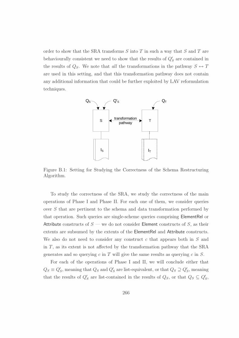
order to show that the SRA transforms S into T in such a way that S and T are
behaviourally consistent we need to show that the results of Q′
S are contained in
the results of QS. We note that all the transformations in the pathway S ↔ T
are used in this setting, and that this transformation pathway does not contain
any additional information that could be further exploited by LAV reformulation
techniques.
transformationpathway
IS
S T
QS QT Q’S
IT
Figure B.1: Setting for Studying the Correctness of the Schema RestructuringAlgorithm.
To study the correctness of the SRA, we study the correctness of the main
operations of Phase I and Phase II. For each one of them, we consider queries
over S that are pertinent to the schema and data transformation performed by
that operation. Such queries are single-scheme queries comprising ElementRel or
Attribute constructs of S — we do not consider Element constructs of S, as their
extents are subsumed by the extents of the ElementRel and Attribute constructs.
We also do not need to consider any construct c that appears both in S and
in T , as its extent is not affected by the transformation pathway that the SRA
generates and so querying c in T will give the same results as querying c in S.
For each of the operations of Phase I and II, we will conclude either that
QS ≡ Q′
S, meaning that QS and Q′
S are list-equivalent, or that QS ⊇ Q′
S, meaning
that the results of Q′
S are list-contained in the results of QS, or that QS ⊆ Q′
S,
266

meaning that the results of QS are list-contained in the results of Q′
S. In the case
that the SRA is not allowed to generate synthetic data, we would expect a number
of the operations performed by the SRA to be lossy with respect to information
content, i.e. that QS ⊇ Q′
S. In the case that the SRA is allowed to generate
synthetic data for some constructs, in order to avoid the loss of information from
their descendant constructs, we would expect that in some cases Q′
S may return
more data than QS, i.e. that QS ⊆ Q′
S .
B.2 Correctness Study
We now study the correctness of the main operations of Phase I and Phase II
when the SRA is applied on a source schema S and a target schema T .
Phase I is applied in the following three types of situations, where 〈〈A, B〉〉 is
an ElementRel construct of S: (i) 〈〈A〉〉 is an ancestor of 〈〈B〉〉 in T , (ii) 〈〈A〉〉 is a
descendant of 〈〈B〉〉 in T , and (iii) 〈〈A〉〉 and 〈〈B〉〉 located in different branches of
T . Phase II is applied in the following three types of situations, where 〈〈A, B〉〉
is an ElementRel construct of T : (i) 〈〈A〉〉 is an ancestor of 〈〈B〉〉 in S, (ii) 〈〈A〉〉 is
a descendant of 〈〈B〉〉 in S, and (iii) 〈〈A〉〉 and 〈〈B〉〉 located in different branches
of S. Since Case (i) for Phase I is the same as Case (i) for Phase II, and simi-
larly for Cases (ii) and (iii), we study the correctness of the three cases for both
phases together. In particular, Section B.2.1 studies the correctness of Case (i) for
Phases I and II (ancestor case), Section B.2.2 studies the correctness of Case (ii)
(descendant case) and Section B.2.3 studies the correctness of Case (iii) (different
branches case).
Phase II is also applied to situations where an Element construct in S is trans-
formed into an Attribute construct in T or vice versa. Section B.2.4 investigates
these two operations, which we termed element-to-attribute and attribute-to-
element transformations in Chapter 5.
267

B.2.1 Ancestor Case
(i) Base Case
Consider the setting illustrated on the left of Figure B.2. We see that S
contains an ElementRel construct 〈〈1, A, B〉〉, whereas in T Element 〈〈A〉〉 is an an-
cestor of 〈〈B〉〉 and T contains constructs 〈〈K〉〉, 〈〈1, A, K〉〉 and 〈〈1, K, B〉〉 that do
not appear in S. Assuming synthetic extent generation is not allowed, the trans-
formation pathway produced by the SRA is given below. Transformations 247
and 248 are produced by operation addElementAndElementRel of Phase II,
and transformations 249 and 250 are produced by operation InsertElementRel
of Phase II.
247 add(〈〈K〉〉,Range Void Any)
248 add(〈〈1,A,K〉〉,Range Void Any)
249 add(〈〈1,K,B〉〉,Range Void Any)
250 delete(〈〈1,A,B〉〉,[{x, y}|{x, d1} ← 〈〈1,A,K〉〉; {d1, y} ← 〈〈1,K,B〉〉])
Consider the following query on S, to return the extent of ElementRel 〈〈1, A, B〉〉:
QS = 〈〈1,A,B〉〉
Using transformation 250, QS is rewritten to the following query on T :
QT =[{x, y}|{x, d1} ← 〈〈1,A,K〉〉; {d1, y} ← 〈〈1,K,B〉〉]
Using transformations 248 and 249, QT is rewritten to Q′
S on S as follows
(assuming lower-bound querying):
Q′
S =Void
In this case, we see that, trivially, QS ⊇ Q′
S.
Assuming now that synthetic extent generation is allowed, the transformation
pathway S → T generated by the SRA is given below. Transformations 251-253
are generated by the application of Phase I on S, and transformation 254 is gen-
erated by operation InsertElementRel of Phase II.
268

251 add(〈〈K〉〉,[y|{x, y, z} ← skolemiseEdge 〈〈1,A,B〉〉 ′K′ ′card2′])
252 add(〈〈1,A,K〉〉,[{x, y}|{x, y, z} ← skolemiseEdge 〈〈1,A,B〉〉 ′K′ ′card2′])
253 add(〈〈1,K,B〉〉,[{y, z}|{x, y, z} ← skolemiseEdge 〈〈1,A,B〉〉 ′K′ ′card2′])
254 delete(〈〈1,A,B〉〉,[{x, y}|{x, d1} ← 〈〈1,A,K〉〉; {d1, y} ← 〈〈1,K,B〉〉])
Given the same query QS as before, and using transformation 254, QS is
rewritten to the following query on T :
QT =[{x, y}|{x, d1} ← 〈〈1,A,K〉〉; {d1, y} ← 〈〈1,K,B〉〉]
Using transformations 252 and 253, QT is rewritten to Q′
S as follows:
Q′
S =[{x, y}|{x, d1} ← [{x, y}|{x, y, z} ← skolemiseEdge 〈〈1,A,B〉〉 ′K′ ′card2′];
{d1, y} ← [{y, z}|{x, y, z} ← skolemiseEdge 〈〈1,A,B〉〉 ′K′ ′card2′]]
Applying unnesting of list comprehensions, this simplifies to:
Q′
S =[{x, y}|{x, d1, z} ← skolemiseEdge 〈〈1,A,B〉〉 ′K′ ′card2′;
{x1, d1, y} ← skolemiseEdge 〈〈1,A,B〉〉 ′K′ ′card2′] (1)
Since skolemiseEdge will always yield the same result given the same input,
and since the two generators in the above comprehension are joined on variable
d1, variables x and x1 must iterate through the same list of instances, and the
same applies for variables z and y. Therefore, x = x1 and z = y and so Q′
S can
be simplified to:
Q′
S =[{x, y}|{x, d1, y} ← skolemiseEdge 〈〈1,A,B〉〉 ′K′ ′card2′]
or, since the first argument of each instance of skolemiseEdge is the initial query:
Q′
S =[{x, y}|{x, d1, y} ← skolemiseEdge QS′K′ ′card2′] (2)
We know from the definition of skolemiseEdge that: (i) the first input argument
(in this case QS) is a query that defines a list of pairs, (ii) the function generates
as many instances as the number of instances of this list of pairs, (iii) the first
and third items in the triples produced by the function are the first and second
items in the input list of pairs without being altered. Since variable d1 is not
used within the comprehension above, Q′
S can be simplified to3:
Q′
S =[{x, y}|{x, y} ← QS]
3In general, given a comprehension containing a generator g of the form {x, y, z} ←skolemiseEdge Q ′K′ ′c′ for some Element label K and some cardinality c, if y is not usedwithin the comprehension, then g can be replaced by generator {x, z} ← Q in that comprehen-sion.
269

Ancestor Case
Tr
A1
1
K
1
B
S
r
A
1
1
B
Ancestor Case – Generalisation
T
A
K
1
1
L
1B
S
r
A
1
1
B
1
r
card1
card2
card3card1card2
Figure B.2: Correctness Study of the SRA: Ancestor Case.
In this case, we see that, trivially, QS ≡ Q′
S.
(ii) Generalisation
Without Synthetic Extent Generation: Consider the setting illustrated on
the right of Figure B.2. This is similar to the setting on the left, but in this case
in T Element constructs 〈〈A〉〉 and 〈〈B〉〉 are separated by two Element constructs,
〈〈K〉〉 and 〈〈L〉〉. Assuming that synthetic extent generation is not allowed, the
transformation pathway produced by the SRA is given below:
255 add(〈〈K〉〉,Range Void Any)
256 add(〈〈1,A,K〉〉,Range Void Any)
257 add(〈〈L〉〉,Range Void Any)
258 add(〈〈1,K,L〉〉,Range Void Any)
259 add(〈〈1,L,B〉〉,Range Void Any)
260 delete(〈〈1,A,B〉〉,[{x, y}|{x, d1} ← 〈〈1,A,K〉〉; {d1, d2} ← 〈〈1,K,L〉〉; {d2, y} ← 〈〈1,L,B〉〉])
270

Given query QS = 〈〈1, A, B〉〉 on S, and using the same argument as before,
we can show that Q′
S =Void, and so QS ⊇ Q′
S.
With Synthetic Extent Generation: Assuming now that synthetic extent
generation is allowed, the transformation pathway S → T generated by the SRA
is given below. Transformations 261-267 are generated by the application of Phase
I on S, and transformation 268 is generated by the application of Phase II on T .
261 add(〈〈K〉〉,[y|{x, y, z} ← skolemiseEdge 〈〈1,A,B〉〉 ′K′ ′card2′])
262 add(〈〈1,A,K〉〉,[{x, y}|{x, y, z} ← skolemiseEdge 〈〈1,A,B〉〉 ′K′ ′card2′])
263 add(〈〈1,K,B〉〉,[{y, z}|{x, y, z} ← skolemiseEdge 〈〈1,A,B〉〉 ′K′ ′card2′])
264 add(〈〈L〉〉,[y|{x, y, z} ← skolemiseEdge 〈〈1,K,B〉〉 ′L′ ′card3′])
265 add(〈〈1,K,L〉〉,[{x, y}|{x, y, z} ← skolemiseEdge 〈〈1,K,B〉〉 ′L′ ′card3′])
266 add(〈〈1,L,B〉〉,[{y, z}|{x, y, z} ← skolemiseEdge 〈〈1,K,B〉〉 ′L′ ′card3′])
267 delete(〈〈1,K,B〉〉,Range Void Any)
268 delete(〈〈1,A,B〉〉,[{x, y}|{x, d1} ← 〈〈1,A,K〉〉; {d1, d2} ← 〈〈1,K,L〉〉; {d2, y} ← 〈〈1,L,B〉〉])
Using the same query QS as before, and using transformation 268, QS is rewrit-
ten to the following query on T :
QT =[{x, y}|{x, d1} ← 〈〈1,A,K〉〉; {d1, d2} ← 〈〈1,K,L〉〉; {d2, y} ← 〈〈1,L,B〉〉]
Using transformations 262, 265 and 266, QT is rewritten to Q′
S as follows:
Q′
S =[{x, y}|{x, d1} ← [{x, y}|{x, y, z} ← skolemiseEdge 〈〈1,A,B〉〉 ′K′ ′card2′];
{d1, d2} ← [{x, y}|{x, y, z} ← skolemiseEdge 〈〈1,K,B〉〉 ′L′ ′card3′];
{d2, y} ← [{y, z}|{x, y, z} ← skolemiseEdge 〈〈1,K,B〉〉 ′L′ ′card3′]]
Applying unnesting of list comprehensions, this simplifies to:
Q′
S =[{x, y}|{x, d1, z} ← skolemiseEdge 〈〈1,A,B〉〉 ′K′ ′card2′;
{d1, d2, z1} ← skolemiseEdge 〈〈1,K,B〉〉 ′L′ ′card3′;
{x1, d2, y} ← skolemiseEdge 〈〈1,K,B〉〉 ′L′ ′card3′]
Since skolemiseEdge will always yield the same result given the same input,
and since the two generators in the above comprehension are joined on variable
d2, the other two pairs of variables must be equal, i.e. d1 = x1 and z1 = y, and
so, Q′
S can be simplified to:
271

Q′
S =[{x, y}|{x, d1, z} ← skolemiseEdge 〈〈1,A,B〉〉 ′K′ ′card2′;
{d1, d2, y} ← skolemiseEdge 〈〈1,K,B〉〉 ′L′ ′card3′]
Using transformation 263, this is rewritten as follows:
Q′
S =[{x, y}|{x, d1, z} ← skolemiseEdge 〈〈1,A,B〉〉 ′K′ ′card2′;
{d1, d2, y} ← skolemiseEdge
[{y, z}|{x, y, z} ← skolemiseEdge 〈〈1,A,B〉〉 ′K′ ′card2′] ′L′ ′card3′] (3)
Since variable d2 is not used within the above comprehension, Q′
S can be
simplified to:
Q′
S =[{x, y}|{x, d1, z} ← skolemiseEdge 〈〈1,A,B〉〉 ′K′ ′card2′;
{d1, y} ← [{y, z}|{x, y, z} ← skolemiseEdge 〈〈1,A,B〉〉 ′K′ ′card2′]]
Applying unnesting of list comprehensions, this simplifies to:
Q′
S =[{x, y}|{x, d1, z} ← skolemiseEdge 〈〈1,A,B〉〉 ′K′ ′card2′;
{x1, d1, y} ← skolemiseEdge 〈〈1,A,B〉〉 ′K′ ′card2′]
Since both occurrences of skolemiseEdge have the same input arguments, and
since the two generators in the above comprehension are joined on variable d1,
we can remove the second generator and simplify Q′
S to:
Q′
S =[{x, y}|{x, d1, y} ← skolemiseEdge 〈〈1,A,B〉〉 ′K′ ′card2′] (4)
or, since QS =〈〈1, A, B〉〉:
Q′
S =[{x, y}|{x, d1, y} ← skolemiseEdge QS′K′ ′card2′]
This equivalence is identical to equivalence (2) given earlier and so QS ≡ Q′
S.
We have investigated the correctness of the SRA when an ElementRel 〈〈1, A, B〉〉
in the source schema is skolemised using a single Element construct (n = 1) and
also 〈〈A〉〉 is an ancestor of 〈〈B〉〉 in the target schema. We then investigated the
correctness of the SRA when n = 2, and we have shown the same conclusions as
for n = 1. This was achieved by eliminating the second and third generators in
Q′
S, thereby reducing the case of n = 2 to the case of n = 1. In general, for n > 1,
Q′
S will contain n generators, and it is clear that each generator after the first
one can be eliminated in the same way as when n = 2. Therefore our conclusions
for the general case of n > 1 are the same as those for the case of n = 1.
272

B.2.2 Descendant Case
(i) Base Case
Consider the setting illustrated on the left of Figure B.3. In this setting, S
contains an ElementRel construct 〈〈1, A, B〉〉, whereas in T Element 〈〈A〉〉 is a de-
scendant of 〈〈B〉〉, and T contains constructs 〈〈K〉〉, 〈〈1, B, K〉〉 and 〈〈1, K, A〉〉 that do
not appear in S. Assuming synthetic extent generation is not allowed, the trans-
formation pathway produced by the SRA is given below. Transformations 270
and 271 are produced by operation addElementAndElementRel of Phase II,
and transformations269 and 272- 28 are produced by operation InsertElemen-
tRel of Phase II.
269 add(〈〈1, r,B〉〉,[{x, y}|{x, d1} ← 〈〈1, r,A〉〉; {d1, y} ← 〈〈1,A,B〉〉])
270 add(〈〈K〉〉,Range Void Any)
271 add(〈〈1,B,K〉〉,Range Void Any)
272 add(〈〈1,K,A〉〉,Range Void Any)
28 delete(〈〈1,A,B〉〉,[{y, x}|{x, u1} ← 〈〈1,B,K〉〉; {u1, y} ← 〈〈1,K,A〉〉])
27 delete(〈〈1, r,A〉〉,[{x, y}|{x, d1} ← 〈〈1, r,B〉〉; {d1, d2} ← 〈〈1,B,K〉〉; {d2, y} ← 〈〈1,K,A〉〉])
Consider the following query on S, to return the extent of ElementRel 〈〈1, A, B〉〉:
QS = 〈〈1,A,B〉〉
Using transformation 28 , QS is rewritten to the following query on T :
QT =[{y, x}|{x, u1} ← 〈〈1,B,K〉〉; {u1, y} ← 〈〈1,K,A〉〉]
Using transformations 271 and 272, QT is rewritten to Q′
S as follows (assuming
lower-bound querying):
Q′
S =Void
In this case, we see that, trivially, QS ⊇ Q′
S.
Assuming now that synthetic extent generation is allowed, the transformation
pathway is as follows:
273

29 add(〈〈K〉〉,[y|{x, y, z} ← skolemiseEdge Q1 ′K′ ′card2′])
30 add(〈〈1,B,K〉〉,[{x, y}|{x, y, z} ← skolemiseEdge Q1 ′K′ ′card2′])
31 add(〈〈1,K,A〉〉,[{y, z}|{x, y, z} ← skolemiseEdge Q1 ′K′ ′card2′])
32 add(〈〈1, r,B〉〉,[{x, y}|{x, d1} ← 〈〈1, r,A〉〉; {d1, y} ← 〈〈1,A,B〉〉])
34 delete(〈〈1,A,B〉〉,Q2)
33 delete(〈〈1, r,A〉〉,[{x, y}|{x, d1} ← 〈〈1, r,B〉〉; {d1, d2} ← 〈〈1,B,K〉〉; {d2, y} ← 〈〈1,K,A〉〉])
In transformations 29 - 31 , Q1 is the query produced by function getInver-
tedElementRelExtent(〈〈A〉〉,〈〈B〉〉), which returns a query that describes the extent
of ‘virtual’ ElementRel 〈〈1, B, A〉〉 and prevents the loss of any instances of 〈〈A〉〉 that
do not have any child instances of 〈〈B〉〉. In transformation 34 , Q2 is the query
produced by function getInvertedElementRelExtent(〈〈B〉〉,〈〈A〉〉). This function is
defined as follows4:
Panel 17: Function getInvertedElementRelExtent(〈〈ep〉〉,〈〈ec〉〉)
/* ****** Function getInvertedElementRelExtent(〈〈ep〉〉,〈〈ec〉〉) ****** */
let q be a path query from 〈〈ep〉〉 to 〈〈ec〉〉 projecting on 〈〈ep〉〉 and 〈〈ec〉〉;96
let Q1 := unnestCollection [Q2|x1← 〈〈ep〉〉], where Q2 is97
if(member [x|{x, y} ← q] x1)98
[{y, x1}|{x, y} ← q; x = x1]99
[{generateUID ′ec′ [x1], x1}];100
return Q1;101
Let us assume first that in S there are no instances of 〈〈A〉〉 that do not have
child instances of 〈〈B〉〉. In such a setting, query Q1 in transformations 29 - 31
would generate the same extent as query [{y, x}|{x, y} ← 〈〈1,A,B〉〉], and query Q2
in transformation 34 would generate the same extent as query [{y, x}|{x, u1} ←
〈〈1,B,K〉〉; {u1, y} ← 〈〈1,K,A〉〉]. Therefore, let us assume that the pathway is as
follows:
4Function getInvertedElementRelExtent was initially defined in Chapter 5 to accept as inputtwo Element constructs 〈〈e1〉〉 and 〈〈e2〉〉, where 〈〈e1〉〉 is the parent of 〈〈e2〉〉. As discussed inChapter 5, it is trivial to extend the original definition for 〈〈e1〉〉 to be, in general, an ancestorof 〈〈e2〉〉. The definition given here is the extension of the definition of Chapter 5.
274

35 add(〈〈K〉〉,[y|{x, y, z} ← skolemiseEdge [{y, x}|{x, y} ← 〈〈1,A,B〉〉] ′K′ ′card2′])
36 add(〈〈1,B,K〉〉,[{x, y}|{x, y, z} ← skolemiseEdge [{y, x}|{x, y} ← 〈〈1,A,B〉〉] ′K′ ′card2′])
37 add(〈〈1,K,A〉〉,[{y, z}|{x, y, z} ← skolemiseEdge [{y, x}|{x, y} ← 〈〈1,A,B〉〉] ′K′ ′card2′])
38 add(〈〈1, r,B〉〉,[{x, y}|{x, d1} ← 〈〈1, r,A〉〉; {d1, y} ← 〈〈1,A,B〉〉])
40 delete(〈〈1,A,B〉〉,[{y, x}|{x, u1} ← 〈〈1,B,K〉〉; {u1, y} ← 〈〈1,K,A〉〉])
39 delete(〈〈1, r,A〉〉,[{x, y}|{x, d1} ← 〈〈1, r,B〉〉; {d1, d2} ← 〈〈1,B,K〉〉; {d2, y} ← 〈〈1,K,A〉〉])
Consider the following query on S, to return the extent of ElementRel 〈〈1, A, B〉〉:
QS = 〈〈1,A,B〉〉
Using transformation 40 , QS is rewritten to the following query on T :
QT =[{y, x}|{x, u1} ← 〈〈1,B,K〉〉; {u1, y} ← 〈〈1,K,A〉〉]
Using transformations 36 and 37 , QT is rewritten to Q′
S as follows:
Q′
S =[{y, x}|{x, u1} ← [{x, y}|{x, y, z} ← skolemiseEdge
[{y, x}|{x, y} ← 〈〈1,A,B〉〉] ′K′ ′card2′];
{u1, y} ← [{y, z}|{x, y, z} ← skolemiseEdge
[{y, x}|{x, y} ← 〈〈1,A,B〉〉] ′K′ ′card2′]]
Applying unnesting of list comprehensions, this simplifies to:
Q′
S =[{y, x}|{x, u1, z} ← skolemiseEdge [{y, x}|{x, y} ← 〈〈1,A,B〉〉] ′K′ ′card2′;
{x1, u1, y} ← skolemiseEdge [{y, x}|{x, y} ← 〈〈1,A,B〉〉] ′K′ ′card2′]
Since skolemiseEdge will always yield the same result given the same input,
and since the two generators in the above comprehension are joined on variable
u1, Q′
S can be simplified to:
Q′
S =[{y, x}|{x, u1, y} ← skolemiseEdge [{y, x}|{x, y} ← 〈〈1,A,B〉〉] ′K′ ′card2′]
or, since QS =〈〈1, A, B〉〉:
Q′
S =[{y, x}|{x, u1, y} ← skolemiseEdge [{y, x}|{x, y} ← QS] ′K′ ′card2′] (5)
Since variable u1 does not contribute to the result of the comprehension,
and since skolemiseEdge does not alter the first and third items in the triples it
produces, Q′
S can be simplified as follows:
Q′
S =[{y, x}|{x, y} ← [{y, x}|{x, y} ← QS]]
Applying unnesting of list comprehensions, this simplifies to:
Q′
S =[{y, x}|{y, x} ← QS]
Therefore, it is trivially the case that QS ≡ Q′
S.
275

Descendant Case
Tr
B1
1
K
1
A
S
r
A
1
1
B
Descendant Case – Generalisation
T
B
K
1
1
L
1
A
S
r
A
1
1
B
1
r
card1
card2
card3card1card2
Figure B.3: Correctness Study of the SRA: Descendant Case.
We now drop the assumption made earlier and investigate the correctness
of the SRA when 〈〈A〉〉 in S contains one or more instances with no child in-
stances of 〈〈B〉〉. In this case, queries Q1 and Q2 in transformations 29 - 31 and
transformation 34 are not equivalent to the queries in transformations 35 - 37
and transformation 40 . In particular, Q1 generates the same pairs as query
[{y, x}|{x, y} ← 〈〈1,A,B〉〉] plus one pair for each instance of 〈〈A〉〉 with no child in-
stances of 〈〈B〉〉. Similarly, Q2 generates the same pairs as query [{y, x}|{x, u1} ←
〈〈1,B,K〉〉; {u1, y} ← 〈〈1,K,A〉〉] plus one pair for each instance of 〈〈B〉〉 with no de-
scendant instances of 〈〈A〉〉. Thus, given the pathway that consists of transforma-
tions 29 - 34 that uses function getInvertedElementRelExtent, we see that QS ⊆ Q′
S,
and so in this case the SRA is incorrect with respect to the notion of behavioural
consistency. However, we note that this is to be expected since we are generating
synthetic instances for some constructs in order to prevent the loss of data from
other constructs, and that the user is able to enable or disable this behaviour of
the SRA.
276

(ii) Generalisation
Without Synthetic Extent Generation: Consider the setting illustrated on
the right of Figure B.3. This is similar to the setting on the left, but in this
case in T Element constructs 〈〈B〉〉 and 〈〈A〉〉 are separated by two Element con-
structs, 〈〈K〉〉 and 〈〈L〉〉. Assuming synthetic extent generation is not allowed,
the transformation pathway produced by the SRA is given below. Transforma-
tions 42 - 45 are produced by operation addElementAndElementRel of Phase
II, and transformations 41 and 46 - 48 are produced by operation InsertElemen-
tRel of Phase II.
41 add(〈〈1, r,B〉〉,[{x, y}|{x, d1} ← 〈〈1, r,A〉〉; {d1, y} ← 〈〈1,A,B〉〉])
42 add(〈〈K〉〉,Range Void Any)
43 add(〈〈1,B,K〉〉,Range Void Any)
44 add(〈〈L〉〉,Range Void Any)
45 add(〈〈1,K,L〉〉,Range Void Any)
46 add(〈〈1,L,A〉〉,Range Void Any)
48 delete(〈〈1,A,B〉〉,[{y, x}|{x, u1} ← 〈〈1,B,K〉〉; {u1, u2} ← 〈〈1,K,L〉〉;
{u2, y} ← 〈〈1,L,A〉〉])
47 delete(〈〈1, r,A〉〉,[{x, y}|{x, d1} ← 〈〈1, r,B〉〉; {d1, d2} ← 〈〈1,B,K〉〉;
{d2, d3} ← 〈〈1,K,L〉〉; {d3, y} ← 〈〈1,L,A〉〉])
Consider the following query on S, to return the extent of ElementRel 〈〈1, A, B〉〉:
QS = 〈〈1,A,B〉〉
Using transformation 48 , QS is rewritten to the following query on T :
QT =[{y, x}|{x, u1} ← 〈〈1,B,K〉〉; {u1, u2} ← 〈〈1,K,L〉〉; {u2, y} ← 〈〈1,L,A〉〉]
Using transformations 43 , 45 and 46 , QT is rewritten to Q′
S as follows (as-
suming lower-bound querying):
Q′
S =Void
In this case, we see that, trivially, QS ⊇ Q′
S.
With Synthetic Extent Generation: Assuming now that synthetic extent
277

generation is allowed, the transformation pathway is as follows:
49 add(〈〈K〉〉,[y|{x, y, z} ← skolemiseEdge Q1 ′K′ ′card2′])
50 add(〈〈1,B,K〉〉,[{x, y}|{x, y, z} ← skolemiseEdge Q1 ′K′ ′card2′])
51 add(〈〈1,K,A〉〉,[{y, z}|{x, y, z} ← skolemiseEdge Q1 ′K′ ′card2′])
52 add(〈〈L〉〉,[y|{x, y, z} ← skolemiseEdge 〈〈1,K,A〉〉 ′L′ ′card3′])
53 add(〈〈1,K,L〉〉,[{x, y}|{x, y, z} ← skolemiseEdge 〈〈1,K,A〉〉 ′L′ ′card3′])
54 add(〈〈1,L,A〉〉,[{y, z}|{x, y, z} ← skolemiseEdge 〈〈1,K,A〉〉 ′L′ ′card3′])
55 delete(〈〈1,K,A〉〉,Range Void Any)
56 add(〈〈1, r,B〉〉,[{x, y}|{x, d1} ← 〈〈1, r,A〉〉; {d1, y} ← 〈〈1,A,B〉〉])
58 delete(〈〈1,A,B〉〉,Q2)
57 delete(〈〈1, r,A〉〉,[{x, y}|{x, d1} ← 〈〈1, r,B〉〉; {d1, d2} ← 〈〈1,B,K〉〉; {d2, y} ← 〈〈1,K,A〉〉])
In transformations 49 - 51 , Q1 is the query produced by function
getInvertedElementRelExtent(〈〈A〉〉,〈〈B〉〉), which returns a query that describes the
extent of ElementRel 〈〈1, B, A〉〉 and prevents the loss of any instances of 〈〈A〉〉 that
do not have any child instances of 〈〈B〉〉. In transformation 58 , Q2 is the query
produced by function getInvertedElementRelExtent(〈〈B〉〉,〈〈A〉〉).
As before, let us assume first that in S there are no instances of 〈〈A〉〉 that do
not have child instances of 〈〈B〉〉. Under this assumption, query Q1 in transforma-
tions 49 - 51 would generate the same extent as query [{y, x}|{x, y} ← 〈〈1,A,B〉〉],
and query Q2 in transformation 58 would generate the same extent as query
[{y, x}|{x, u1} ← 〈〈B,K〉〉; {u1, u2} ← 〈〈K,L〉〉; {u2, y} ← 〈〈L,A〉〉]. Therefore, let us as-
sume that the pathway is as follows:
278

59 add(〈〈K〉〉,[y|{x, y, z} ← skolemiseEdge [{y, x}|{x, y} ← 〈〈1,A,B〉〉] ′K′ ′card2′])
60 add(〈〈1,B,K〉〉,[{x, y}|{x, y, z} ← skolemiseEdge [{y, x}|{x, y} ← 〈〈1,A,B〉〉] ′K′ ′card2′])
61 add(〈〈1,K,A〉〉,[{y, z}|{x, y, z} ← skolemiseEdge [{y, x}|{x, y} ← 〈〈1,A,B〉〉] ′K′ ′card2′])
62 add(〈〈L〉〉,[y|{x, y, z} ← skolemiseEdge 〈〈1,K,A〉〉 ′L′ ′card3′])
63 add(〈〈1,K,L〉〉,[{x, y}|{x, y, z} ← skolemiseEdge 〈〈1,K,A〉〉 ′L′ ′card3′])
64 add(〈〈1,L,A〉〉,[{y, z}|{x, y, z} ← skolemiseEdge 〈〈1,K,A〉〉 ′L′ ′card3′])
65 delete(〈〈1,K,A〉〉,Range Void Any)
66 add(〈〈1, r,B〉〉,[{x, y}|{x, d1} ← 〈〈1, r,A〉〉; {d1, y} ← 〈〈1,A,B〉〉])
68 delete(〈〈1,A,B〉〉,[{y, x}|{x, u1} ← 〈〈1,B,K〉〉; {u1, u2} ← 〈〈1,K,L〉〉; {u2, y} ← 〈〈1,L,A〉〉])
67 delete(〈〈1, r,A〉〉,[{x, y}|{x, d1} ← 〈〈1, r,B〉〉; {d1, d2} ← 〈〈1,B,K〉〉; {d2, y} ← 〈〈1,K,A〉〉])
Consider the following query on S, to return the extent of ElementRel 〈〈1, A, B〉〉:
QS = 〈〈1,A,B〉〉
Using transformation 68 , QS is rewritten to the following query on T :
QT =[{y, x}|{x, u1} ← 〈〈1,B,K〉〉; {u1, u2} ← 〈〈1,K,L〉〉; {u2, y} ← 〈〈1,L,A〉〉]
Using transformations 60 , 63 and 64 , QT is rewritten to Q′
S as follows:
Q′
S =[{y, x}|{x, u1} ← [{x, y}|{x, y, z} ← skolemiseEdge
[{y, x}|{x, y} ← 〈〈1,A,B〉〉] ′K′ ′card2′];
{u1, u2} ← [{x, y}|{x, y, z} ← skolemiseEdge 〈〈1,K,A〉〉 ′L′ ′card3′];
{u2, y} ← [{y, z}|{x, y, z} ← skolemiseEdge 〈〈1,K,A〉〉 ′L′ ′card3′]]
Applying unnesting of list comprehensions, this simplifies to:
Q′
S =[{y, x}|{x, u1, z} ← skolemiseEdge [{y, x}|{x, y} ← 〈〈1,A,B〉〉] ′K′ ′card2′;
{u1, u2, z1} ← skolemiseEdge 〈〈1,K,A〉〉 ′L′ ′card3′;
{x1, u2, y} ← skolemiseEdge 〈〈1,K,A〉〉 ′L′ ′card3′]
Since skolemiseEdge will always yield the same result given the same input,
and since last two generators in the above comprehension are joined on variable
u2, Q′
S can be simplified to:
Q′
S =[{y, x}|{x, u1, z} ← skolemiseEdge [{y, x}|{x, y} ← 〈〈1,A,B〉〉] ′K′ ′card2′;
{u1, u2, y} ← skolemiseEdge 〈〈1,K,A〉〉 ′L′ ′card3′]
Using transformation 61 , this is rewritten as follows:
Q′
S =[{y, x}|{x, u1, z} ← skolemiseEdge [{y, x}|{x, y} ← 〈〈1,A,B〉〉] ′K′ ′card2′;
{u1, u2, y} ← skolemiseEdge
279

[{y, z}|{x, y, z} ← skolemiseEdge [{y, x}|{x, y} ← 〈〈1,A,B〉〉] ′K′ ′card2′] ′L′ ′card3′]
We notice that Q′
S is similar to (3), except for the variable names and the
first input argument to the first and third occurrence of function skolemiseEdge.
Also, we have shown earlier that (3) can be simplified to (4). Therefore, using
the simplification of (3) to (4) as a simplification template, Q′
S can be rewritten
as follows:
Q′
S =[{y, x}|{x, u1, y} ← skolemiseEdge [{y, x}|{x, y} ← 〈〈1,A,B〉〉] ′K′ ′card2′]
or, since QS =〈〈1, A, B〉〉:
Q′
S =[{y, x}|{x, u1, y} ← skolemiseEdge [{y, x}|{x, y} ← QS] ′K′ ′card2′]
This equivalence is identical to (5), for which we know that QS ≡ Q′
S, and so
the same conclusion holds for this setting as well.
We now drop the assumption made earlier and investigate the correctness
of the SRA when 〈〈A〉〉 in S contains one or more instances with no child in-
stances of 〈〈B〉〉. In this case, queries Q1 and Q2 in transformations 49 - 51 and
transformation 58 are not equivalent to the queries in transformations 59 - 61
and transformation 68 . In particular, Q1 generates the same pairs as query
[{y, x}|{x, y} ← 〈〈1,A,B〉〉] plus one pair for each instance of 〈〈A〉〉 with no child in-
stances of 〈〈B〉〉. Similarly, Q2 generates the same pairs as query [{y, x}|{x, u1} ←
〈〈1,B,K〉〉; {u1, u2} ← 〈〈1,K,L〉〉; {u2, y} ← 〈〈1,L,A〉〉] plus one pair for each instance of
〈〈B〉〉 with no descendant instances of 〈〈A〉〉. Thus, given the pathway that consists
of transformations 49 - 58 that uses function getInvertedElementRelExtent, we see
that QS ⊆ Q′
S. Again, this is to be expected since we are generating synthetic
instances for some constructs in order to prevent the loss of data from other con-
structs.
We have investigated the correctness of the SRA when an ElementRel 〈〈1, A, B〉〉
in the source schema is skolemised using a single Element construct (n = 1) and
also 〈〈A〉〉 is a descendant of 〈〈B〉〉 in the target schema. We then investigated the
correctness of the SRA when n = 2, and we have derived the same conclusions as
for n = 1. This was achieved by eliminating the second and third generators in
Q′
S, thereby reducing the case of n = 2 to the case of n = 1. In general, for n > 1,
280

Q′
S will contain n generators, and it is clear that each generator after the first
one can be eliminated in the same way as when n = 2. Therefore our conclusions
for the general case of n > 1 are the same as for the case of n = 1.
Finally, we note that the SRA handles the case when n = 0 using Phase II,
since no skolemisation takes place. However, Phase II uses function getInvert-
edElementRelExtent, and so the investigation is similar to the case when n = 1,
and reaches the same conclusions.
B.2.3 Different Branches Case
(i) Base Case
Consider the setting illustrated on the left of Figure B.4. In this setting,
〈〈A〉〉 and 〈〈B〉〉 share a parent-child relationship in S, but are located in different
branches in the T . Assuming synthetic extent generation is not allowed, the trans-
formation pathway S → T generated by the SRA is given below. Transformations
69 - 74 are generated by the application of Phase II on S, and transformations
75 - 76 are generated by the application of Phase II on T .
69 add(〈〈K〉〉,Range Void Any)
70 add(〈〈1,C,K〉〉,Range Void Any)
71 add(〈〈1,K,A〉〉,Range Void Any)
72 add(〈〈L〉〉,Range Void Any)
73 add(〈〈2,C,L〉〉,Range Void Any)
74 add(〈〈1,L,B〉〉,Range Void Any)
76 delete(〈〈1,A,B〉〉,[{x, z}|{x, y} ← [{y, x}|{x, u1} ← 〈〈1,C,K〉〉; {u1, y} ← 〈〈1,K,A〉〉];
{y, z} ← [{x, y}|{x, d1} ← 〈〈2,C,L〉〉; {d1, y} ← 〈〈1,L,B〉〉]])
75 delete(〈〈1,C,A〉〉,[{x, y}|{x, d1} ← 〈〈1,C,K〉〉; {d1, y} ← 〈〈1,K,A〉〉])
Consider the following query on S, to return the extent of ElementRel 〈〈1, A, B〉〉:
QS = 〈〈1,A,B〉〉
Using transformation 76 , QS is rewritten to the following query on T :
QT =[{x, z}|{x, y} ← [{y, x}|{x, u1} ← 〈〈1,C,K〉〉; {u1, y} ← 〈〈1,K,A〉〉];
281

{y, z} ← [{x, y}|{x, d1} ← 〈〈2,C,L〉〉; {d1, y} ← 〈〈1,L,B〉〉]]
Using transformations 70 , 71 , 73 and 74 , QT is rewritten to Q′
S on S as
follows (assuming lower-bound querying):
Q′
S =Void
In this case, we see that, trivially, QS ⊇ Q′
S.
Assuming now that synthetic extent generation is allowed, the transformation
pathway is as follows:
77 add(〈〈K〉〉,[y|{x, y, z} ← skolemiseEdge 〈〈1,C,A〉〉 ′K′ ′card2′])
78 add(〈〈1,C,K〉〉,[{x, y}|{x, y, z} ← skolemiseEdge 〈〈1,C,A〉〉 ′K′ ′card2′])
79 add(〈〈1,K,A〉〉,[{y, z}|{x, y, z} ← skolemiseEdge 〈〈1,C,A〉〉 ′K′ ′card2′])
80 add(〈〈L〉〉,[y|{x, y, z} ← skolemiseEdge Q3 ′L′ ′card3′])
81 add(〈〈2,C,L〉〉,[{x, y}|{x, y, z} ← skolemiseEdge Q3 ′L′ ′card3′])
82 add(〈〈1,L,B〉〉,[{y, z}|{x, y, z} ← skolemiseEdge Q3 ′L′ ′card3′])
84 delete(〈〈1,A,B〉〉,[{x, z}|{x, y} ← Q4;
{y, z} ← [{x, y}|{x, d1} ← 〈〈2,C,L〉〉; {d1, y} ← 〈〈1,L,B〉〉]])
83 delete(〈〈1,C,A〉〉,[{x, y}|{x, d1} ← 〈〈1,C,K〉〉; {d1, y} ← 〈〈1,K,A〉〉])
where Q3 = [{x, z}|{x, y} ← 〈〈1,C,A〉〉; {y, z} ← 〈〈1,A,B〉〉] is a query that defines the
extent of ‘virtual’ ElementRel 〈〈1, C, B〉〉 in S so that 〈〈1, C, B〉〉 can be skolemised
using Element 〈〈L〉〉, and where Q4 is a query that defines the extent of ‘virtual’
ElementRel 〈〈1, A, C〉〉 in T using function getInvertedElementRelExtent.
Let us assume first that query Q4 in transformation 84 generates the same
extent as query [{y, x}|{x, u1} ← 〈〈1,C,K〉〉; {u1, y} ← 〈〈1,K,A〉〉]. Therefore, let us
assume that the pathway is as follows:
282

85 add(〈〈K〉〉,[y|{x, y, z} ← skolemiseEdge 〈〈1,C,A〉〉 ′K′ ′card2′])
86 add(〈〈1,C,K〉〉,[{x, y}|{x, y, z} ← skolemiseEdge 〈〈1,C,A〉〉 ′K′ ′card2′])
87 add(〈〈1,K,A〉〉,[{y, z}|{x, y, z} ← skolemiseEdge 〈〈1,C,A〉〉 ′K′ ′card2′])
88 add(〈〈L〉〉,[y|{x, y, z} ← skolemiseEdge Q3 ′L′ ′card3′])
89 add(〈〈2,C,L〉〉,[{x, y}|{x, y, z} ← skolemiseEdge Q3 ′L′ ′card3′])
90 add(〈〈1,L,B〉〉,[{y, z}|{x, y, z} ← skolemiseEdge Q3 ′L′ ′card3′])
92 delete(〈〈1,A,B〉〉,[{x, z}|{x, y} ← [{y, x}|{x, u1} ← 〈〈1,C,K〉〉; {u1, y} ← 〈〈1,K,A〉〉];
{y, z} ← [{x, y}|{x, d1} ← 〈〈2,C,L〉〉; {d1, y} ← 〈〈1,L,B〉〉]])
91 delete(〈〈1,C,A〉〉,[{x, y}|{x, d1} ← 〈〈1,C,K〉〉; {d1, y} ← 〈〈1,K,A〉〉])
Consider the following query on S, to return the extent of ElementRel 〈〈1, A, B〉〉:
QS = 〈〈1,A,B〉〉
Using transformation 92 , QS is rewritten to the following query on T :
QT =[{x, z}|{x, y} ← [{y, x}|{x, u1} ← 〈〈1,C,K〉〉; {u1, y} ← 〈〈1,K,A〉〉];
{y, z} ← [{x, y}|{x, d1} ← 〈〈2,C,L〉〉; {d1, y} ← 〈〈1,L,B〉〉]]
Applying unnesting of list comprehensions, this simplifies to:
QT =[{x, z}|{y, u1} ← 〈〈1,C,K〉〉; {u1, x} ← 〈〈1,K,A〉〉;
{y, d1} ← 〈〈2,C,L〉〉; {d1, z} ← 〈〈1,L,B〉〉]
Using transformations 86 , 87 , 89 and 90 , QT is rewritten to Q′
S as follows:
Q′
S =[{x, z}|{y, u1} ← [{x, y}|{x, y, z} ← skolemiseEdge 〈〈1,C,A〉〉 ′K′ ′card2′];
{u1, x} ← [{y, z}|{x, y, z} ← skolemiseEdge 〈〈1,C,A〉〉 ′K′ ′card2′];
{y, d1} ← [{x, y}|{x, y, z} ← skolemiseEdge Q3 ′L′ ′card3′];
{d1, z} ← [{y, z}|{x, y, z} ← skolemiseEdge Q3 ′L′ ′card3′]]
Applying unnesting of list comprehensions, this simplifies to:
Q′
S =[{x, z}|{y, u1, z1} ← skolemiseEdge 〈〈1,C,A〉〉 ′K′ ′card2′;
{x1, u1, x} ← skolemiseEdge 〈〈1,C,A〉〉 ′K′ ′card2′;
{y, d1, z2} ← skolemiseEdge Q3 ′L′ ′card3′;
{x2, d1, z} ← skolemiseEdge Q3 ′L′ ′card3′] (6)
Since skolemiseEdge will always yield the same result given the same input,
and since the first and second generators in the above comprehension are joined
on variable u1, one of them can be removed, and the same applies for the third
and fourth generators, which are joined on variable d1. Therefore, Q′
S can be
283

simplified to:
Q′
S =[{x, z}|{y, u1, x} ← skolemiseEdge 〈〈1,C,A〉〉 ′K′ ′card2′;
{y, d1, z} ← skolemiseEdge Q3 ′L′ ′card3′]
Since variable u1 is not used within the comprehension, the first generator
can be replaced by the generator {y, x} ← 〈〈1,C,A〉〉. Similarly, the body of the
second generator can be replaced by query Q3, which we know is [{x, z}|{x, y} ←
〈〈1,C,A〉〉; {y, z} ← 〈〈1,A,B〉〉]. Therefore, Q′
S is simplified to:
Q′
S =[{x, z}|{y, x} ← 〈〈1,C,A〉〉;
{y, z} ← [{x, z}|{x, y} ← 〈〈1,C,A〉〉; {y, z} ← 〈〈1,A,B〉〉]]
Applying unnesting of list comprehensions, this simplifies to:
Q′
S =[{x, z}|{y, x} ← 〈〈1,C,A〉〉; {y, y1} ← 〈〈1,C,A〉〉; {y1, z} ← 〈〈1,A,B〉〉]
Clearly the second generator can be removed:
Q′
S =[{x, z}|{y, x} ← 〈〈1,C,A〉〉; {x, z} ← 〈〈1,A,B〉〉]
Since in S Element 〈〈C〉〉 is the parent of 〈〈A〉〉, and 〈〈A〉〉 is the parent of 〈〈B〉〉,
it is not possible for the first generator to produce an instance that cannot be
joined with an instance of the second generator (and therefore constrain it), so:
Q′
S =[{x, z}|{x, z} ← QS]
In this case, we see that, trivially, QS ≡ Q′
S.
We now drop the assumption made earlier and investigate the correctness of
the SRA when query Q4 in transformation 84 is not equivalent to the query in
transformation 92 . In particular, Q4 generates the same pairs as the query in
transformation 92 plus one pair for each instance of 〈〈C〉〉 with no child instances
of 〈〈A〉〉. Thus, given the pathway that consists of transformations 85 - 92 that
uses query Q4, we see that QS ⊆ Q′
S.
(ii) Generalisation
Without Synthetic Extent Generation: Consider the setting illustrated on
the right of Figure B.4. This is similar to the setting on the left, but in this case
in T Element constructs 〈〈C〉〉 and 〈〈A〉〉 are separated by two Element constructs,
284

Different Branches Case
TrS
K L
2 1
1
C
1 1A B
r
C1
1
A
1
B
Different Branches Case – Generalisation
T
C
S
M N
2 1
1 1
A B
r
C1
1
A
1
B
1
r
K L
1 1
card1
card3
card1
card3
card5
card2
card2
card4
Figure B.4: Correctness Investigation of the SRA: Different Branches Case.
〈〈K〉〉 and 〈〈M〉〉, and similarly Element constructs 〈〈C〉〉 and 〈〈B〉〉 are separated by
two Element constructs, 〈〈L〉〉 and 〈〈N〉〉. Assuming synthetic extent generation is
not allowed, the transformation pathway S → T generated by the SRA is given
below. Transformations 93 -102 are generated by the application of Phase II on
S, and transformations 103-104 are generated by the application of Phase II on T .
93 add(〈〈K〉〉,Range Void Any)
94 add(〈〈1,C,K〉〉,Range Void Any)
95 add(〈〈M〉〉,Range Void Any)
96 add(〈〈1,K,M〉〉,Range Void Any)
285

97 add(〈〈1,M,A〉〉,Range Void Any)
98 add(〈〈L〉〉,Range Void Any)
99 add(〈〈2,C,L〉〉,Range Void Any)
100 add(〈〈N〉〉,Range Void Any)
101 add(〈〈1,L,N〉〉,Range Void Any)
102 add(〈〈1,N,B〉〉,Range Void Any)
104 delete(〈〈1,A,B〉〉,[{x, z}|
{x, y} ← [{y, x}|{x, u1} ← 〈〈1,C,K〉〉; {u1, u2} ← 〈〈1,K,M〉〉; {u2, y} ← 〈〈1,M,A〉〉];
{y, z} ← [{x, y}|{x, d1} ← 〈〈2,C,L〉〉; {d1, d2} ← 〈〈1,L,N〉〉; {d2, y} ← 〈〈1,N,B〉〉]])
103 delete(〈〈1,C,A〉〉,[{x, y}|{x, d1} ← 〈〈1,C,K〉〉; {d1, d2} ← 〈〈1,K,M〉〉; {d2, y} ← 〈〈1,M,A〉〉])
Consider the following query on S, to return the extent of ElementRel 〈〈1, A, B〉〉:
QS = 〈〈1,A,B〉〉
Using transformation 104, QS is rewritten to the following query on T :
QT =[{x, z}|
{x, y} ← [{y, x}|{x, u1} ← 〈〈1,C,K〉〉; {u1, u2} ← 〈〈1,K,M〉〉; {u2, y} ← 〈〈1,M,A〉〉];
{y, z} ← [{x, y}|{x, d1} ← 〈〈2,C,L〉〉; {d1, d2} ← 〈〈1,L,N〉〉; {d2, y} ← 〈〈1,N,B〉〉]]
Using transformations 94 , 96 , 97 , 99 , 101 and 102, QT is rewritten to Q′
S on
S as follows (assuming lower-bound querying):
Q′
S =Void
In this case, we see that, trivially, QS ⊇ Q′
S.
With Synthetic Extent Generation: Assuming now that synthetic extent
generation is allowed, the transformation pathway is as follows:
105 add(〈〈K〉〉,[y|{x, y, z} ← skolemiseEdge 〈〈1,C,A〉〉 ′K′ ′card2′])
106 add(〈〈1,C,K〉〉,[{x, y}|{x, y, z} ← skolemiseEdge 〈〈1,C,A〉〉 ′K′ ′card2′])
107 add(〈〈1,K,A〉〉,[{y, z}|{x, y, z} ← skolemiseEdge 〈〈1,C,A〉〉 ′K′ ′card2′])
108 add(〈〈M〉〉,[y|{x, y, z} ← skolemiseEdge 〈〈1,K,A〉〉 ′M′ ′card4′])
109 add(〈〈1,K,M〉〉,[{x, y}|{x, y, z} ← skolemiseEdge 〈〈1,K,A〉〉 ′M′ ′card4′])
110 add(〈〈1,M,A〉〉,[{y, z}|{x, y, z} ← skolemiseEdge 〈〈1,K,A〉〉 ′M′ ′card4′])
111 delete(〈〈1,K,A〉〉,Range Void Any)
112 add(〈〈L〉〉,[y|{x, y, z} ← skolemiseEdge Q3 ′L′ ′card3′])
286

113 add(〈〈2,C,L〉〉,[{x, y}|{x, y, z} ← skolemiseEdge Q3 ′L′ ′card3′])
114 add(〈〈1,L,B〉〉,[{y, z}|{x, y, z} ← skolemiseEdge Q3 ′L′ ′card3′])
115 add(〈〈N〉〉,[y|{x, y, z} ← skolemiseEdge 〈〈1,L,B〉〉 ′N′ ′card5′])
116 add(〈〈1,L,N〉〉,[{x, y}|{x, y, z} ← skolemiseEdge 〈〈1,L,B〉〉 ′N′ ′card5′])
117 add(〈〈1,N,B〉〉,[{y, z}|{x, y, z} ← skolemiseEdge 〈〈1,L,B〉〉 ′N′ ′card5′])
118 delete(〈〈1,L,B〉〉,Range Void Any)
120 delete(〈〈1,A,B〉〉,[{x, z}|
{x, y} ← Q5;
{y, z} ← [{x, y}|{x, d1} ← 〈〈2,C,L〉〉; {d1, d2} ← 〈〈1,L,N〉〉; {d2, y} ← 〈〈1,N,B〉〉]])
119 delete(〈〈1,C,A〉〉,[{x, y}|{x, d1} ← 〈〈1,C,K〉〉; {d1, d2} ← 〈〈1,K,M〉〉; {d2, y} ← 〈〈1,M,A〉〉])
where Q3 = [{x, z}|{x, y} ← 〈〈1,C,A〉〉; {y, z} ← 〈〈1,A,B〉〉] is a query that defines the
extent of ‘virtual’ ElementRel 〈〈1, C, B〉〉 in S so that 〈〈1, C, B〉〉 can be skolemised
using Element 〈〈L〉〉, and where Q5 is a query that defines the extent of ‘virtual’
ElementRel 〈〈1, A, C〉〉 in T using function getInvertedElementRelExtent. Notice that
we use the same label for query Q3 as in the previous case, since the two queries
are the same.
Let us assume first that query Q5 in transformation 84 generates the same ex-
tent as query [{y, x}|{x, u1} ← 〈〈1,C,K〉〉; {u1, u2} ← 〈〈1,K,M〉〉; {u2, y} ← 〈〈1,M,A〉〉].
Therefore, let us assume that the pathway is as follows:
121 add(〈〈K〉〉,[y|{x, y, z} ← skolemiseEdge 〈〈1,C,A〉〉 ′K′ ′card2′])
122 add(〈〈1,C,K〉〉,[{x, y}|{x, y, z} ← skolemiseEdge 〈〈1,C,A〉〉 ′K′ ′card2′])
123 add(〈〈1,K,A〉〉,[{y, z}|{x, y, z} ← skolemiseEdge 〈〈1,C,A〉〉 ′K′ ′card2′])
124 add(〈〈M〉〉,[y|{x, y, z} ← skolemiseEdge 〈〈1,K,A〉〉 ′M′ ′card4′])
125 add(〈〈1,K,M〉〉,[{x, y}|{x, y, z} ← skolemiseEdge 〈〈1,K,A〉〉 ′M′ ′card4′])
126 add(〈〈1,M,A〉〉,[{y, z}|{x, y, z} ← skolemiseEdge 〈〈1,K,A〉〉 ′M′ ′card4′])
127 delete(〈〈1,K,A〉〉,Range Void Any)
128 add(〈〈L〉〉,[y|{x, y, z} ← skolemiseEdge Q3 ′L′ ′card3′])
129 add(〈〈2,C,L〉〉,[{x, y}|{x, y, z} ← skolemiseEdge Q3 ′L′ ′card3′])
130 add(〈〈1,L,B〉〉,[{y, z}|{x, y, z} ← skolemiseEdge Q3 ′L′ ′card3′])
131 add(〈〈N〉〉,[y|{x, y, z} ← skolemiseEdge 〈〈1,L,B〉〉 ′N′ ′card5′])
132 add(〈〈1,L,N〉〉,[{x, y}|{x, y, z} ← skolemiseEdge 〈〈1,L,B〉〉 ′N′ ′card5′])
287

133 add(〈〈1,N,B〉〉,[{y, z}|{x, y, z} ← skolemiseEdge 〈〈1,L,B〉〉 ′N′ ′card5′])
134 delete(〈〈1,L,B〉〉,Range Void Any)
120 delete(〈〈1,A,B〉〉,[{x, z}|
{x, y} ← [{y, x}|{x, u1} ← 〈〈1,C,K〉〉; {u1, u2} ← 〈〈1,K,M〉〉; {u2, y} ← 〈〈1,M,A〉〉];
{y, z} ← [{x, y}|{x, d1} ← 〈〈2,C,L〉〉; {d1, d2} ← 〈〈1,L,N〉〉; {d2, y} ← 〈〈1,N,B〉〉]])
119 delete(〈〈1,C,A〉〉,[{x, y}|{x, d1} ← 〈〈1,C,K〉〉; {d1, d2} ← 〈〈1,K,L〉〉; {d2, y} ← 〈〈1,L,A〉〉])
Consider the following query on S, to return the extent of ElementRel 〈〈1, A, B〉〉:
QS = 〈〈1,A,B〉〉
Using transformation 120, QS is rewritten to the following query on T :
QT =[{x, z}|
{x, y} ← [{y, x}|{x, u1} ← 〈〈1,C,K〉〉; {u1, u2} ← 〈〈1,K,M〉〉; {u2, y} ← 〈〈1,M,A〉〉];
{y, z} ← [{x, y}|{x, d1} ← 〈〈2,C,L〉〉; {d1, d2} ← 〈〈1,L,N〉〉; {d2, y} ← 〈〈1,N,B〉〉]]
Applying unnesting of list comprehensions, this simplifies to:
QT =[{x, z}|{y, u1} ← 〈〈1,C,K〉〉; {u1, u2} ← 〈〈1,K,M〉〉; {u2, x} ← 〈〈1,M,A〉〉;
{y, d1} ← 〈〈2,C,L〉〉; {d1, d2} ← 〈〈1,L,N〉〉; {d2, z} ← 〈〈1,N,B〉〉]
Using transformations 122, 125, 126, 129, 132, 133 , QT is rewritten to Q′
S as
follows:
Q′
S =[{x, z}|{y, u1} ← [{x, y}|{x, y, z} ← skolemiseEdge 〈〈1,C,A〉〉 ′K′ ′card2′];
{u1, u2} ← [{x, y}|{x, y, z} ← skolemiseEdge 〈〈1,K,A〉〉 ′M′ ′card4′];
{u2, x} ← [{y, z}|{x, y, z} ← skolemiseEdge 〈〈1,K,A〉〉 ′M′ ′card4′];
{y, d1} ← [{x, y}|{x, y, z} ← skolemiseEdge Q3 ′L′ ′card3′];
{d1, d2} ← [{x, y}|{x, y, z} ← skolemiseEdge 〈〈1,L,B〉〉 ′N′ ′card5′];
{d2, z} ← [{y, z}|{x, y, z} ← skolemiseEdge 〈〈1,L,B〉〉 ′N′ ′card5′]]
Applying unnesting of list comprehensions, this simplifies to:
Q′
S =[{x, z}|{y, u1, z1} ← skolemiseEdge 〈〈1,C,A〉〉 ′K′ ′card2′;
{u1, u2, z2} ← skolemiseEdge 〈〈1,K,A〉〉 ′M′ ′card4′];
{x1, u2, x} ← skolemiseEdge 〈〈1,K,A〉〉 ′M′ ′card4′];
{y, d1, z3} ← skolemiseEdge Q3 ′L′ ′card3′];
{d1, d2, z4} ← skolemiseEdge 〈〈1,L,B〉〉 ′N′ ′card5′];
{x2, d2, z} ← skolemiseEdge 〈〈1,L,B〉〉 ′N′ ′card5′]]
The second and third generators are joined on variable u2, and so one of
288

them can be removed, and the same applies for the fifth and sixth generators.
Therefore, Q′
S can be rewritten as follows:
Q′
S =[{x, z}|{y, u1, z1} ← skolemiseEdge 〈〈1,C,A〉〉 ′K′ ′card2′;
{u1, u2, x} ← skolemiseEdge 〈〈1,K,A〉〉 ′M′ ′card4′;
{y, d1, z3} ← skolemiseEdge Q3 ′L′ ′card3′;
{d1, d2, z} ← skolemiseEdge 〈〈1,L,B〉〉 ′N′ ′card5′]
Since variables u2 and d2 are not used within the comprehension above, Q′
S
is simplified to:
Q′
S =[{x, z}|{y, u1, z1} ← skolemiseEdge 〈〈1,C,A〉〉 ′K′ ′card2′;
{u1, x} ← 〈〈1,K,A〉〉;
{y, d1, z3} ← skolemiseEdge Q3 ′L′ ′card3′;
{d1, z} ← 〈〈1,L,B〉〉]
Using transformations 123 and 130, Q′
S is rewritten as follows:
Q′
S =[{x, z}|{y, u1, z1} ← skolemiseEdge 〈〈1,C,A〉〉 ′K′ ′card2′;
{u1, x} ← [{y, z}|{x, y, z} ← skolemiseEdge 〈〈1,C,A〉〉 ′K′ ′card2′];
{y, d1, z3} ← skolemiseEdge Q3 ′L′ ′card3′;
{d1, z} ← [{y, z}|{x, y, z} ← skolemiseEdge Q3 ′L′ ′card3′]]
Applying unnesting of list comprehensions, this simplifies to:
Q′
S =[{x, z}|{y, u1, z1} ← skolemiseEdge 〈〈1,C,A〉〉 ′K′ ′card2′;
{x1, u1, x} ← skolemiseEdge 〈〈1,C,A〉〉 ′K′ ′card2′;
{y, d1, z3} ← skolemiseEdge Q3 ′L′ ′card3′;
{x2, d1, z} ← skolemiseEdge Q3 ′L′ ′card3′] (7)
This equivalence is identical to (6), for which we know that QS ≡ Q′
S, and so
the same equivalence holds in this setting as well.
We now drop the assumption made earlier and investigate the correctness of
the SRA when query Q5 transformation 120 is not equivalent to the query in
transformation 120. In particular, Q5 generates the same pairs as the query in
transformation 120 plus one pair for each instance of 〈〈C〉〉 with no child instances
of 〈〈A〉〉. Thus, given the pathway that consists of transformations 105-120 that
uses query Q5, we see that QS ⊆ Q′
S.
289

We have investigated the correctness of the SRA when a source schema that
contains two Element constructs 〈〈A〉〉 and 〈〈B〉〉 that share a parent-child relation-
ship is transformed into a schema where 〈〈A〉〉 and 〈〈B〉〉 are located in different
branches and their common ancestor 〈〈C〉〉 is the same Element that is the parent
of 〈〈A〉〉 in S. In particular, we first investigated the case where a single Element
construct (n = 1) exists between 〈〈C〉〉 and each of these Element constructs in
the target schema. We then investigated the correctness of the SRA when n = 2,
and we have shown the same conclusions as for n = 1. This was achieved by
reducing the case of n = 2 to the case of n = 1. In general, it is clear that it
is possible to reduce each case where n > 1 to the case where n = 1, therefore
the conclusions for the general case of n > 1 are the same as those for the case
of n = 1. We also note that we would reach the same conclusions even if in T
the number of Element constructs between 〈〈C〉〉 and 〈〈A〉〉 is different than the
number of Element constructs between 〈〈C〉〉 and 〈〈B〉〉.
Finally, we note that the SRA handles the case when n = 0 using Phase II,
since no skolemisation takes place. However, Phase II uses function getInvert-
edElementRelExtent, and so the investigation is similar to the case when n = 1,
and reaches the same conclusions.
B.2.4 Element-to-attribute transformation
Consider the element-to-attribute transformation illustrated on the left of Fig-
ure B.5. Assuming that synthetic extent generation is not allowed, the transfor-
mation pathway produced by the SRA is given below. The transformations in
the pathway are a result of operations addAttribute and addElementAndEle-
mentRel of Phase II of the SRA.
121 addAtt(〈〈e, a〉〉,Range Void Any)
124 deleteER(〈〈1, a,Text〉〉,Range Void Any)
123 deleteER(〈〈1, e, a〉〉,Range Void Any)
122 deleteEl(〈〈a〉〉,Range Void Any)
290

Consider the following query on S, to return the extent of Element 〈〈e〉〉 to-
gether with its associated 〈〈Text〉〉 instances:
QS =[{x, z}|{x, y} ← 〈〈1, e, a〉〉; {y, z} ← 〈〈1, a,Text〉〉]
Using transformations 123 and 124, QT and Q′
S result in Void (assuming lower-
bound querying), and so it is trivially the case that QS ⊇ Q′
S.
Now, assuming that synthetic extent generation is allowed, the transforma-
tion pathway S → T generated by the SRA is as follows. The transforma-
tions in the pathway are a result of operations Element2Attribute and At-
tribute2Element of Phase II of the SRA.
125 addAtt(〈〈e, a〉〉,[{x, z}|{x, y} ← 〈〈1, e, a〉〉; {y, z} ← 〈〈1, a,Text〉〉])
128 deleteER(〈〈1, a,Text〉〉,[{y, z}|{x, y, z} ← skolemiseEdge 〈〈e, a〉〉 ′a′ ′1− 1′])
127 deleteER(〈〈1, e, a〉〉,[{x, y}|{x, y, z} ← skolemiseEdge 〈〈e, a〉〉 ′a′ ′1− 1′])
126 deleteEl(〈〈a〉〉,[y|{x, y, z} ← skolemiseEdge 〈〈e, a〉〉 ′a′ ′1− 1′])
Consider the following query on S, to return the extent of Element 〈〈e〉〉 to-
gether with its associated 〈〈Text〉〉 instances:
QS =[{x, z}|{x, y} ← 〈〈1, e, a〉〉; {y, z} ← 〈〈1, a,Text〉〉]
Using transformations 127 and 128, QS is rewritten to the following query on
T :
QT =[{x, z}|{x, y} ← [{x, y}|{x, y, z} ← skolemiseEdge 〈〈e, a〉〉 ′a′ ′1− 1′];
{y, z} ← [{y, z}|{x, y, z} ← skolemiseEdge 〈〈e, a〉〉 ′a′ ′1− 1′]]
Applying unnesting of list comprehensions, this simplifies to:
QT =[{x, z}|{x, y, z1} ← skolemiseEdge 〈〈e, a〉〉 ′a′ ′1− 1′;
{x1, y, z} ← skolemiseEdge 〈〈e, a〉〉 ′a′ ′1− 1′]
Since skolemiseEdge will always yield the same result given the same input,
and since the two generators in the above comprehension are joined on variable
y, QT can be simplified to:
QT =[{x, z}|{x, y, z} ← skolemiseEdge 〈〈e, a〉〉 ′a′ ′1− 1′]
Since variable y is not used within the above comprehension, QT can be sim-
plified to:
QT =[{x, z}|{x, z} ← 〈〈e, a〉〉]
291

Using transformation 125, QT is rewritten to Q′
S on S as follows:
Q′
S =[{x, z}|{x, z} ← [{x, z}|{x, y} ← 〈〈1, e, a〉〉; {y, z} ← 〈〈1, a,Text〉〉]]
Applying unnesting of list comprehensions, this simplifies to:
Q′
S =[{x, z}|{x, y} ← 〈〈1, e, a〉〉; {y, z} ← 〈〈1, a,Text〉〉]
This is the original query QS, and so it is trivially the case that QS ≡ Q′
S.
Phase II - Element-to-Attribute
S
Phase II - Attribute-to-Element
S T
r
e
1
T r
e1
1
a
1
Text
a
r
e1
1
a
1
Text
r
e
1
a
Figure B.5: Correctness Study of the SRA: Element-to-Attribute and Attribute-to-Element Cases.
Finally, we note that the investigation of the attribute-to-element operation is
similar to that for the element-to-attribute operation, due to the bidirectionality
of BAV pathways and the fact that the element-to-attribute operation of the SRA
is the inverse of the attribute-to-element operation. To illustrate, the following
is the transformation pathway for the setting shown on the right of Figure B.5
when synthetic extent generation is not allowed:
129 addEl(〈〈a〉〉,Range Void Any)
130 addER(〈〈1, e, a〉〉,Range Void Any)
131 addER(〈〈1, a,Text〉〉,Range Void Any)
132deleteAtt(〈〈e, a〉〉,Range Void Any)
and we see that it is the reverse of the transformation pathway for the element-
to-attribute operation when synthetic data generation is not allowed (see trans-
formations 121-124).
292

When synthetic extent generation is allowed, the transformation pathway is:
133 addEl(〈〈a〉〉,[y|{x, y, z} ← skolemiseEdge 〈〈e, a〉〉 ′a′ ′1− 1′])
134 addER(〈〈1, e, a〉〉,[{x, y}|{x, y, z} ← skolemiseEdge 〈〈e, a〉〉 ′a′ ′1− 1′])
135 addER(〈〈1, a,Text〉〉,[{y, z}|{x, y, z} ← skolemiseEdge 〈〈e, a〉〉 ′a′ ′1− 1′])
136deleteAtt(〈〈e, a〉〉,[{x, z}|{x, y} ← 〈〈1, e, a〉〉; {y, z} ← 〈〈1, a,Text〉〉])
and we see that it is the reverse of the transformation pathway for the element-
to-attribute operation when synthetic data generation is allowed (see transforma-
tion 125-128.
B.3 Discussion
We have studied the correctness of the main operations of our schema restructur-
ing algorithm (SRA) using the notion of behavioural consistency. We have shown
that when it does not generate synthetic data, the SRA is behaviourally consis-
tent but suffers from loss of data. When it does generate synthetic data, the SRA
is behaviourally consistent for the ancestor and element-to-attribute cases, but is
not behaviourally consistent for the descendant and different branches cases. In
all cases of synthetic extent generation, however, the SRA avoids the loss of data.
In conclusion, depending on the application setting, the user can choose be-
tween consistency and loss of data in some cases, or inconsistency in some cases
and preservation of data in all cases.
293
Appendix C
Single Ontology Service
Reconciliation Files
This appendix provides some of the documents used for, or produced in, the
process of the reconciliation of the services of the workflow getIPIEntry →
getInterProEntry → getPfamEntry. In particular, we provide the documents
related to the outputs of the second and the third services; those related to the
inputs of the second and third services are included in the main text of the thesis.
We first list the documents related to the output of service getIPIEntry. Sec-
tion C.1 lists the output of service getIPIEntry given IPI accession IPI00015171,
i.e. a UniProt-style flat file representation of an IPI entry. Section C.2 lists the
XML version of Section C.1, produced by our IPI flat-file-to-XML format con-
verter, as discussed in Chapter 7. Section C.3 lists the XMLDSS schema au-
tomatically derived from the UniProt XML Schema at the time, version 1.27,
listed in Section C.4 (the latest version of this schema can be found at ftp:
//ftp.ebi.ac.uk/pub/databases/uniprot/knowledgebase/uniprot.xsd).
We then list the documents related to the output of service getInterProEntry.
Section C.5 lists the output of service getIPIEntry given InterPro accession
IPR003959, i.e. an XML file corresponding to the DTD listed in Section C.6.
This DTD is used to automatically derive the XMLDSS schema listed in Sec-
tion C.7.
294

C.1 IPI Entry IPI00015171 (UniProt Flat-File
Version)
ID IPI00015171.4 IPI; PRT; 128 AA.
AC IPI00015171; IPI00784015;
DT 01-OCT-2001 (IPI Human rel. 2.00, Created)
DT 04-SEP-2005 (IPI Human rel. 3.10, Last sequence update)
DE SIMILAR TO AFG3-LIKE PROTEIN 1.
OS Homo sapiens (Human).
OC Eukaryota; Metazoa; Chordata; Craniata; Vertebrata; Euteleostomi;
OC Mammalia; Eutheria; Primates; Catarrhini; Hominidae; Homo.
OX NCBI_TaxID=9606;
CC -!- CHROMOSOME: 16.
CC -!- START CO-ORDINATE: 88566495.
CC -!- END CO-ORDINATE: 88590519.
CC -!- STRAND: 1.
DR UniProtKB/Swiss-Prot; O43931; AFG31_HUMAN; -.
DR Vega; OTTHUMP00000080121; OTTHUMG00000072815; M.
DR ENSEMBL; ENSP00000373622; ENSG00000167540; -.
DR H-InvDB; HIT000013102; HIX0013375; -.
DR UniParc; UPI000059D3F9; -; -.
DR HGNC; 314; AFG3L1; -.
DR Entrez Gene; 172; AFG3L1; -.
DR UniGene; Hs.534773; -; -.
DR trome; HTR002494; -; -.
DR UTRdb; BB153156; -; 5’UTR.
DR UTRdb; BB281690; -; 5’UTR.
DR UTRdb; BB394662; -; 5’UTR.
DR RZPD; Hs.534773; -; Clones and other research material.
DR CleanEx; HS_AFG3L1; -; -.
DR InterPro; IPR003959; AAA_ATPase_core.
DR Pfam; PF00004; AAA; 1.
SQ SEQUENCE 128 AA; 13733 MW; B7335211CD58D03B CRC64;
MRPGRFHRQI YTGPPYIKGR SSIFKVHLRP LKLDKSLNKD TLARKLAVLT PGFPGVHHTP
GQGAPLRTVP APGAAALHPG AALRPHVHDA RGPGSRAAVL RVDHYGGSGR PEEGHPECLR
PGCAVWGE
//
295

C.2 IPI Entry IPI00015171 (XML Version)
<uniprot>
<entry created="2001-10-01" modified="2005-09-04" version="3.10">
<accession>IPI00015171</accession>
<accession>IPI00784015</accession>
<organism key="1">
<name scientific="Homo sapiens"/> <name common="Human"/>
<lineage>
<taxon>Eukaryota</taxon>
<taxon>Metazoa</taxon>
<taxon>Chordata</taxon>
<taxon>Craniata</taxon>
<taxon>Vertebrata</taxon>
<taxon>Euteleostomi</taxon>
<taxon>Mammalia</taxon>
<taxon>Eutheria</taxon>
<taxon>Primates</taxon>
<taxon>Catarrhini</taxon>
<taxon>Hominidae</taxon>
<taxon>Homo</taxon>
</lineage>
<dbReference id="9606" key="2" type="NCBI_TaxID">
</dbReference>
</organism>
<!-- CHROMOSOME: 16. -->
<!-- START CO-ORDINATE: 88566495. -->
<!-- END CO-ORDINATE: 88590519. -->
<!-- STRAND: 1. -->
<dbReference id="O43931" key="3" type="Swiss-Prot">
<property type="entry id" value="AFG31_HUMAN"> </property>
<property type="master" value="0"> </property>
</dbReference>
<dbReference id="OTTHUMP00000080121" key="4" type="Vega">
<property type="gene id" value="OTTHUMG00000072815"> </property>
<property type="master" value="1"> </property>
</dbReference>
296

<dbReference id="ENSP00000373622" key="5" type="ENSEMBL">
<property type="gene id" value="ENSG00000167540"/>
<property type="master" value="0"/>
</dbReference>
<dbReference id="HIT000013102" key="6" type="H-InvDB">
<property type="H-Inv cluster id" value="HIX0013375"/>
<property type="master" value="0"/>
</dbReference>
<dbReference id="UPI000059D3F9" key="7" type="UniParc">
</dbReference>
<dbReference id="HGNC:314" key="8" type="HGNC">
<property type="HGNC official gene symbol" value="AFG3L1"/>
</dbReference>
<dbReference id="172" key="9" type="Entrez Gene">
<property type="default gene symbol" value="AFG3L1"/></dbReference>
<dbReference id="Hs.534773" key="10" type="UniGene"/>
<dbReference id="HTR002494" key="11" type="trome"/>
<dbReference id="BB153156" key="12" type="UTRdb"/>
<dbReference id="BB281690" key="13" type="UTRdb"/>
<dbReference id="BB394662" key="14" type="UTRdb"/>
<dbReference id="Hs.534773" key="15" type="RZPD"/>
<dbReference id="HS_AFG3L1" key="16" type="CleanEx"/>
<dbReference id="IPR003959" key="17" type="InterPro">
<property type="entry name" value="AAA_ATPase_core"/>
<property type="master" value="0"/>
</dbReference>
<dbReference id="PF00004" key="18" type="Pfam">
<property type="method name" value="AAA"/>
<property type="number of hits" value="1"/>
</dbReference>
<sequence crc64="B7335211CD58D03B" length="128" mass="13733">
MRPGRFHRQIYTGPPYIKGRSSIFKVHLRPLKLDKSLNKDTLARKLAVLT
PGFPGVHHTPGQGAPLRTVPAPGAAALHPGAALRPHVHDARGPGSRAAVL
RVDHYGGSGRPEEGHPECLRPGCAVWGE
</sequence>
</entry>
</uniprot>
297

C.3 UniProt XMLDSS
<uniprot>
<entry created="text" dataset="text" modified="text" version="text">
<accession> text </accession>
<name> text </name>
<protein evidence="text" type="text">
<name evidence="text" ref="text"> text </name>
<domain>
<name evidence="text" ref="text"> text </name>
</domain>
<component>
<name evidence="text" ref="text"> text </name>
</component>
</protein>
<gene>
<name/>
</gene>
<organism key="text">
<name/>
<dbReference evidence="text" id="text" key="text" type="text">
<property type="text" value="text"/>
</dbReference>
<lineage>
<taxon> text </taxon>
</lineage>
</organism>
<organismHost key="text">
<name/>
<dbReference evidence="text" id="text" key="text" type="text">
<property type="text" value="text"/>
</dbReference>
<lineage>
<taxon> text </taxon>
</lineage>
</organismHost>
<geneLocation evidence="text" type="text">
298

<name/>
</geneLocation>
<reference evidence="text" key="text">
<citation city="text" country="text" date="text"
db="text" first="text" institute="text"
last="text" name="text" number="text"
publisher="text" type="text" volume="text">
<title> text </title>
<editorList>
<person name="text"/>
<consortium name="text"/>
</editorList>
<authorList>
<person name="text"/>
<consortium name="text"/>
</authorList>
<locator> text </locator>
<dbReference evidence="text" id="text" key="text" type="text">
<property type="text" value="text"/>
</dbReference>
<citingCitation city="text" country="text" date="text"
db="text" first="text" institute="text"
last="text" name="text" number="text"
publisher="text" type="text" volume="text">
<title> text </title>
<editorList>
<person name="text"/>
<consortium name="text"/>
</editorList>
<authorList>
<person/>
<consortium/>
</authorList>
<locator> text </locator>
<dbReference/>
<citingCitation city="text" country="text" date="text"
db="text" first="text" institute="text"
299

last="text" name="text" number="text"
publisher="text" type="text" volume="text">
<title> text </title>
<editorList>
<person/>
<consortium/>
</editorList>
<authorList>
<person/>
<consortium/>
</authorList>
<locator> text </locator>
<dbReference/>
<citingCitation city="text" country="text" date="text"
db="text" first="text" institute="text"
last="text" name="text" number="text"
publisher="text" type="text" volume="text">
<title> text </title>
<editorList/>
<authorList/>
<locator> text </locator>
<dbReference/>
<citingCitation/>
</citingCitation>
</citingCitation>
</citingCitation>
</citation>
</reference>
<comment error="text" evidence="text" locationType="text" mass="text"
method="text" name="text" status="text" type="text">
<text> text </text>
<absorption>
<max> text </max>
<text> text </text>
</absorption>
<kinetics>
<KM> text </KM>
300

<Vmax> text </Vmax>
<text> text </text>
</kinetics>
<phDependence> text </phDependence>
<redoxPotential> text </redoxPotential>
<temperatureDependence> text </temperatureDependence>
<link uri="text"/>
<location sequence="text">
<begin position="text" status="text"/>
<end position="text" status="text"/>
<position position="text" status="text"/>
</location>
<event evidence="text" namedIsoforms="text" type="text">
text
</event>
<comment> text </comment>
<isoform>
<id> text </id>
<name/>
<sequence ref="text" type="text"/>
<note evidence="text"> text </note>
</isoform>
<interactant intactId="text">
<id> text </id>
<label> text </label>
</interactant>
<organismsDiffer> text </organismsDiffer>
<experiments> text </experiments>
<note> text </note>
</comment>
<dbReference/>
<keyword evidence="text" id="text"> text </keyword>
<feature description="text" evidence="text" id="text" ref="text"
status="text" type="text">
<original> text </original>
<variation> text </variation>
<location sequence="text">
301

<begin position="text" status="text"/>
<end position="text" status="text"/>
<position position="text" status="text"/>
</location>
</feature>
<evidence attribute="text" category="text" date="text"
key="text" type="text"/>
<sequence checksum="text" length="text" mass="text"
modified="text" version="text">
text </sequence>
</entry>
<copyright>
text
</copyright>
</uniprot>
302

C.4 UniProt XML Schema
<?xml version="1.0" encoding="UTF-8"?>
<!--*****************************************************************************
UniProt Knowledgebase
Version: $Revision: 1.27 $
Date: $Date: 2006/05/24 13:37:45 $
Copyright (c) 2003 UniProt consortium
All rights reserved.
*******************************************************************************-->
<xs:schema targetNamespace="http://uniprot.org/uniprot"
xmlns:xs="http://www.w3.org/2001/XMLSchema" xmlns="http://uniprot.org/uniprot"
elementFormDefault="qualified">
<!-- XML Schema definition for the UniProt XML format
Tested with:
-XSV (XML Schema Validator), http://www.ltg.ed.ac.uk/~ht/xsv-status.html
-SQC (XML Schema Quality Checker), http://www.alphaworks.ibm.com/tech/xmlsqc
-MSV (Multi-Schema XML Validator),
http://wwws.sun.com/software/xml/developers/multischema/
-XMLSpy, http://www.xmlspy.com/
-->
<!-- Name definition begins -->
<xs:complexType name="proteinNameType">
<xs:annotation>
<xs:documentation>The name type is used for protein names occuring in an
entry, which are represented in a flat file as DE lines.</xs:documentation>
</xs:annotation>
<xs:simpleContent>
<xs:extension base="xs:string">
<xs:attribute name="evidence" type="xs:string" use="optional"/>
<xs:attribute name="ref" type="xs:string" use="optional">
<xs:annotation>
<xs:documentation>This is referring to a possible EC number
(ENZYME database cross reference).</xs:documentation>
</xs:annotation>
</xs:attribute>
</xs:extension>
</xs:simpleContent>
</xs:complexType>
<xs:complexType name="geneNameType">
<xs:annotation>
<xs:documentation>The gene name type is used for gene information.
</xs:documentation>
</xs:annotation>
<xs:simpleContent>
<xs:extension base="xs:string">
303

<xs:attribute name="evidence" type="xs:string" use="optional"/>
<xs:attribute name="type" use="required">
<xs:simpleType>
<xs:restriction base="xs:string">
<xs:enumeration value="primary"/>
<xs:enumeration value="synonym"/>
<xs:enumeration value="ordered locus"/>
<xs:enumeration value="ORF"/>
</xs:restriction>
</xs:simpleType>
</xs:attribute>
</xs:extension>
</xs:simpleContent>
</xs:complexType>
<xs:complexType name="organismNameType">
<xs:annotation>
<xs:documentation>The name type is used for source organism names.
</xs:documentation>
</xs:annotation>
<xs:simpleContent>
<xs:extension base="xs:string">
<xs:attribute name="type" use="required">
<xs:simpleType>
<xs:restriction base="xs:string">
<xs:enumeration value="common"/>
<xs:enumeration value="full"/>
<xs:enumeration value="scientific"/>
<xs:enumeration value="synonym"/>
<xs:enumeration value="abbreviation"/>
</xs:restriction>
</xs:simpleType>
</xs:attribute>
</xs:extension>
</xs:simpleContent>
</xs:complexType>
<xs:complexType name="statusType">
<xs:annotation>
<xs:documentation>The status attribute provides a known/unknown flag.
</xs:documentation>
</xs:annotation>
<xs:simpleContent>
<xs:extension base="xs:string">
<xs:attribute name="status" use="optional" default="known">
<xs:simpleType>
<xs:restriction base="xs:string">
<xs:enumeration value="known"/>
<xs:enumeration value="unknown"/>
304

</xs:restriction>
</xs:simpleType>
</xs:attribute>
</xs:extension>
</xs:simpleContent>
</xs:complexType>
<!-- Name definition ends -->
<!-- Definition of the protein begins -->
<xs:complexType name="proteinType">
<xs:annotation>
<xs:documentation>The protein element stores all the information found in
the DE line of a flatfile entry.</xs:documentation>
</xs:annotation>
<xs:sequence>
<xs:element name="name" type="proteinNameType" maxOccurs="unbounded"/>
<xs:element name="domain" minOccurs="0" maxOccurs="unbounded">
<xs:annotation>
<xs:documentation>The domain list is equivalent to the INCLUDES
section of the DE line.</xs:documentation>
</xs:annotation>
<xs:complexType>
<xs:sequence>
<xs:element name="name" type="proteinNameType" maxOccurs="unbounded"/>
</xs:sequence>
</xs:complexType>
</xs:element>
<xs:element name="component" minOccurs="0" maxOccurs="unbounded">
<xs:annotation>
<xs:documentation>The component list is equivalent to the CONTAINS
section of the DE line.</xs:documentation>
</xs:annotation>
<xs:complexType>
<xs:sequence>
<xs:element name="name" type="proteinNameType" maxOccurs="unbounded"/>
</xs:sequence>
</xs:complexType>
</xs:element>
</xs:sequence>
<xs:attribute name="type">
<xs:simpleType>
<xs:restriction base="xs:NMTOKEN">
<xs:enumeration value="fragment"/>
<xs:enumeration value="fragments"/>
<xs:enumeration value="version1"/>
<xs:enumeration value="version2"/>
</xs:restriction>
</xs:simpleType>
305
</xs:attribute>
<xs:attribute name="evidence" type="xs:string" use="optional">
<xs:annotation>
<xs:documentation>This contains all evidences that are connected
to the complete DE line.</xs:documentation>
</xs:annotation>
</xs:attribute>
</xs:complexType>
<!-- Definition of the protein ends -->
<!-- Definition of the geneLocation begins -->
<xs:complexType name="geneLocationType">
<xs:annotation>
<xs:documentation>Defines the locations/origins of the shown
sequence (OG line).</xs:documentation>
</xs:annotation>
<xs:sequence>
<xs:element name="name" type="statusType" minOccurs="0"/>
</xs:sequence>
<xs:attribute name="type" use="required">
<xs:simpleType>
<xs:restriction base="xs:string">
<xs:enumeration value="apicoplast"/>
<xs:enumeration value="chloroplast"/>
<xs:enumeration value="cyanelle"/>
<xs:enumeration value="hydrogenosome"/>
<xs:enumeration value="mitochondrion"/>
<xs:enumeration value="non-photosynthetic plastid"/>
<xs:enumeration value="nucleomorph"/>
<xs:enumeration value="plasmid"/>
<xs:enumeration value="plastid"/>
</xs:restriction>
</xs:simpleType>
</xs:attribute>
<xs:attribute name="evidence" type="xs:string" use="optional"/>
</xs:complexType>
<!-- Definition of the geneLocation ends -->
<!-- Citation type section begins -->
<xs:complexType name="citationType">
<xs:annotation>
<xs:documentation>The citation type stores all information about a citation.
The equivalent information in the flatfile can be found in the RA (authors),
RT (title), RX (PubMed/MEDLINE/DOI IDs) and RL (citation location information
such journal name, volume numbers, pages, etc.) lines.</xs:documentation>
</xs:annotation>
<xs:sequence>
<xs:element name="title" type="xs:string" minOccurs="0">
<xs:annotation>
306

<xs:documentation>The title of the citation. Stored in the RT line in
the flatfile format.</xs:documentation>
</xs:annotation>
</xs:element>
<xs:element name="editorList" type="nameListType" minOccurs="0">
<xs:annotation>
<xs:documentation>The editors of a book. Stored in the RL line in the
flatfile format. Only valid for books. Example:
RL (In) Magnusson S., Ottesen M., Foltmann B., Dano K.,
RL Neurath H. (eds.);
RL Regulatory proteolytic enzymes and their inhibitors, pp.163-172,
RL Pergamon Press, New York (1978).
</xs:documentation>
</xs:annotation>
</xs:element>
<xs:element name="authorList" type="nameListType" minOccurs="0">
<xs:annotation>
<xs:documentation>The authors of the citation. Stored in the RA line in
the flatfile format, except for citing citation where it is stored in
the RL line. Example (standard citation):
RA Galinier A., Bleicher F., Negre D., Perriere G., Duclos B.,
RA Cozzone A.J., Cortay J.-C.;
Example (citing citation):
RL Unpublished results, cited by:
RL Shelnutt J.A., Rousseau D.L., Dethmers J.K., Margoliash E.;
RL Biochemistry 20:6485-6497(1981).
</xs:documentation>
</xs:annotation>
</xs:element>
<xs:element name="locator" type="xs:string" minOccurs="0">
<xs:annotation>
<xs:documentation>The location information of an electronic (or online)
article. It is in most cases the unprocessed RL line of an electronic
article. Examples:
RL (In) Plant Gene Register PGR98-023.
RL (In) Worm Breeder’s Gazette 15(3):34(1998).
</xs:documentation>
</xs:annotation>
</xs:element>
<xs:element name="dbReference" type="dbReferenceType" minOccurs="0"
maxOccurs="unbounded">
<xs:annotation>
<xs:documentation/>
</xs:annotation>
</xs:element>
<xs:element name="citingCitation" type="citationType" minOccurs="0">
<xs:annotation>
307

<xs:documentation>Used by type: unpublished results.</xs:documentation>
</xs:annotation>
</xs:element>
</xs:sequence>
<xs:attribute name="type" use="required">
<xs:simpleType>
<xs:restriction base="xs:string">
<xs:enumeration value="book"/>
<xs:enumeration value="journal article"/>
<xs:enumeration value="online journal article"/>
<xs:enumeration value="patent"/>
<xs:enumeration value="submission"/>
<xs:enumeration value="thesis"/>
<xs:enumeration value="unpublished observations"/>
<xs:enumeration value="unpublished results"/>
</xs:restriction>
</xs:simpleType>
</xs:attribute>
<xs:attribute name="date" use="optional">
<xs:simpleType>
<xs:union memberTypes="xs:date xs:gYearMonth xs:gYear"/>
</xs:simpleType>
</xs:attribute>
<xs:attribute name="name" type="xs:string" use="optional"/>
<xs:attribute name="volume" type="xs:string" use="optional"/>
<xs:attribute name="first" type="xs:string" use="optional"/>
<xs:attribute name="last" type="xs:string" use="optional"/>
<xs:attribute name="publisher" type="xs:string" use="optional"/>
<xs:attribute name="city" type="xs:string" use="optional"/>
<xs:attribute name="db" type="xs:string" use="optional"/>
<xs:attribute name="country" type="xs:string" use="optional"/>
<xs:attribute name="number" type="xs:string" use="optional">
<xs:annotation>
<xs:documentation>Used by type: patent.</xs:documentation>
</xs:annotation>
</xs:attribute>
<xs:attribute name="institute" type="xs:string" use="optional">
<xs:annotation>
<xs:documentation>Used by type: thesis.</xs:documentation>
</xs:annotation>
</xs:attribute>
</xs:complexType>
<xs:complexType name="consortiumType">
<xs:attribute name="name" type="xs:string" use="required"/>
</xs:complexType>
<xs:complexType name="personType">
<xs:attribute name="name" type="xs:string" use="required"/>
308

</xs:complexType>
<xs:complexType name="nameListType">
<xs:choice maxOccurs="unbounded">
<xs:element name="person" type="personType"/>
<xs:element name="consortium" type="consortiumType"/>
</xs:choice>
</xs:complexType>
<!-- Definitions for SPTr’s additional citation information begins -->
<xs:complexType name="sourceDataType">
<xs:annotation>
<xs:documentation>Contains all information about the source this citation is
referring to (RC line). The used child-element names are equivalent to the
tokens used in the RC line. Examples:
RC STRAIN=Sprague-Dawley; TISSUE=Liver;
RC STRAIN=Holstein; TISSUE=Lymph node, and Mammary gland;
RC PLASMID=IncFII R100;
</xs:documentation>
</xs:annotation>
<xs:choice maxOccurs="unbounded">
<xs:element name="species">
<xs:complexType>
<xs:simpleContent>
<xs:extension base="xs:string">
<xs:attribute name="ref" type="xs:string" use="optional"/>
</xs:extension>
</xs:simpleContent>
</xs:complexType>
</xs:element>
<xs:element name="strain">
<xs:complexType>
<xs:simpleContent>
<xs:extension base="xs:string">
<xs:attribute name="evidence" type="xs:string" use="optional"/>
</xs:extension>
</xs:simpleContent>
</xs:complexType>
</xs:element>
<xs:element name="plasmid">
<xs:complexType>
<xs:simpleContent>
<xs:extension base="xs:string">
<xs:attribute name="evidence" type="xs:string" use="optional"/>
</xs:extension>
</xs:simpleContent>
</xs:complexType>
</xs:element>
<xs:element name="transposon">
309

<xs:complexType>
<xs:simpleContent>
<xs:extension base="xs:string">
<xs:attribute name="evidence" type="xs:string" use="optional"/>
</xs:extension>
</xs:simpleContent>
</xs:complexType>
</xs:element>
<xs:element name="tissue">
<xs:complexType>
<xs:simpleContent>
<xs:extension base="xs:string">
<xs:attribute name="evidence" type="xs:string" use="optional"/>
</xs:extension>
</xs:simpleContent>
</xs:complexType>
</xs:element>
</xs:choice>
</xs:complexType>
<xs:group name="sptrCitationGroup">
<xs:annotation>
<xs:documentation>Groups the scope (RP lines) and source data (RC lines)
lists.</xs:documentation>
</xs:annotation>
<xs:sequence>
<xs:element name="scope" type="xs:string" maxOccurs="unbounded">
<xs:annotation>
<xs:documentation>Contains a scope regarding a citation. There is
no classification yet. (RP lines).</xs:documentation>
</xs:annotation>
</xs:element>
<xs:element name="source" type="sourceDataType" minOccurs="0">
<xs:annotation>
<xs:documentation>Contains all information about the source this
citation is referring to (RC line).</xs:documentation>
</xs:annotation>
</xs:element>
</xs:sequence>
</xs:group>
<!-- Definitions for SPTr’s additional citation information ends -->
<xs:complexType name="referenceType">
<xs:annotation>
<xs:documentation>Stores all information of the reference block in SPTr
(RN, RP, RC, RX, RA, RT and RL line).</xs:documentation>
</xs:annotation>
<xs:sequence>
<xs:element name="citation" type="citationType"/>
310

<xs:group ref="sptrCitationGroup"/>
</xs:sequence>
<xs:attribute name="evidence" type="xs:string" use="optional"/>
<xs:attribute name="key" type="xs:string" use="required"/>
</xs:complexType>
<!-- Citation type section ends -->
<!-- Comment definition begins -->
<xs:group name="bpcCommentGroup">
<xs:sequence>
<xs:element name="absorption" minOccurs="0" maxOccurs="1">
<xs:complexType>
<xs:sequence>
<xs:element name="max" type="xs:string" minOccurs="0" maxOccurs="1"/>
<xs:element name="text" type="xs:string" minOccurs="0" maxOccurs="1"/>
</xs:sequence>
</xs:complexType>
</xs:element>
<xs:element name="kinetics" minOccurs="0" maxOccurs="1">
<xs:complexType>
<xs:sequence>
<xs:element name="KM" type="xs:string" minOccurs="0"
maxOccurs="unbounded"/>
<xs:element name="Vmax" type="xs:string" minOccurs="0"
maxOccurs="unbounded"/>
<xs:element name="text" type="xs:string" minOccurs="0"
maxOccurs="1"/>
</xs:sequence>
</xs:complexType>
</xs:element>
<xs:element name="phDependence" type="xs:string" minOccurs="0" maxOccurs="1"/>
<xs:element name="redoxPotential" type="xs:string" minOccurs="0" maxOccurs="1"/>
<xs:element name="temperatureDependence" type="xs:string" minOccurs="0"
maxOccurs="1"/>
</xs:sequence>
</xs:group>
<xs:complexType name="commentType">
<xs:annotation>
<xs:documentation>The comment element stores all information found in the
CC lines of the flatfile format. If there is a defined structure to the CC
comment, the extracted is displayed in the various defined attributes and
child-elements. See the documentation of these attributes/elements for more
details.</xs:documentation>
</xs:annotation>
<xs:sequence>
<xs:element name="text" type="xs:string" minOccurs="0" maxOccurs="1">
<xs:annotation>
311

<xs:documentation>If a CC line type does not have a defined structure,
the text of this comment is stored in the element.</xs:documentation>
</xs:annotation>
</xs:element>
<xs:group ref="bpcCommentGroup"/>
<xs:choice minOccurs="0" maxOccurs="1">
<xs:sequence>
<xs:element name="link" minOccurs="0" maxOccurs="unbounded">
<xs:annotation>
<xs:documentation>This stored the URIs defined in the WWW and
FTP tokens of the database (online information in the XML format)
CC comment type.</xs:documentation>
</xs:annotation>
<xs:complexType>
<xs:attribute name="uri" type="xs:anyURI" use="required"/>
</xs:complexType>
</xs:element>
</xs:sequence>
<xs:sequence>
<xs:element name="location" type="locationType" minOccurs="0"
maxOccurs="unbounded">
<xs:annotation>
<xs:documentation>The information of the mass spectrometry comment
is stored in the attributes:
-molWeight (molecular weight)
-mwError (error of the molecular weight)
-msMethod (the method used for the mass spectrometry)
-range (which amino acids were messured. It’s not mentioned if the
complete sequence as shown in the entry was measured)
</xs:documentation>
</xs:annotation>
</xs:element>
</xs:sequence>
<xs:sequence>
<xs:element name="event" type="eventType" minOccurs="1" maxOccurs="4"/>
<xs:element name="comment" type="xs:string" minOccurs="0" maxOccurs="1"/>
<xs:element name="isoform" type="isoformType" minOccurs="0"
maxOccurs="unbounded"/>
</xs:sequence>
<xs:sequence>
<xs:element name="interactant" type="interactantType" minOccurs="2"
maxOccurs="2"/>
<xs:element name="organismsDiffer" type="xs:boolean" minOccurs="1"
default="false"/>
<xs:element name="experiments" type="xs:integer" minOccurs="1"
maxOccurs="1"/>
</xs:sequence>
312

</xs:choice>
<xs:element name="note" type="xs:string" minOccurs="0" maxOccurs="1">
<xs:annotation>
<xs:documentation>If a CC line type contains a "NOTE=", the text of
that note is stored in this element.</xs:documentation>
</xs:annotation>
</xs:element>
</xs:sequence>
<xs:attribute name="name" type="xs:string" use="optional">
<xs:annotation>
<xs:documentation>States the name of the online information if there
is one.</xs:documentation>
</xs:annotation>
</xs:attribute>
<xs:attribute name="mass" type="xs:float" use="optional">
<xs:annotation>
<xs:documentation>First the molecular weight which has been
determined.</xs:documentation>
</xs:annotation>
</xs:attribute>
<xs:attribute name="error" type="xs:string" use="optional">
<xs:annotation>
<xs:documentation>The accuracy with which the molecular weight has been
measured.</xs:documentation>
</xs:annotation>
</xs:attribute>
<xs:attribute name="method" type="xs:string" use="optional">
<xs:annotation>
<xs:documentation>The method which has been used. Common values are
ELECTROSPRAY, MALDI, FAB and PLASMA DESORPTION.</xs:documentation>
</xs:annotation>
</xs:attribute>
<xs:attribute name="status" type="xs:string" use="optional">
<xs:annotation>
<xs:documentation>Some comments have a status reflecting their reliability.
Common values are BY SIMILARITY, POTENTIAL and PROBABLE.</xs:documentation>
</xs:annotation>
</xs:attribute>
<xs:attribute name="locationType" type="xs:string" use="optional">
<xs:annotation>
<xs:documentation>Defines the type of the location where RNA editing takes
place. Common values are "Displayed", "Not_applicable" and "Undetermined".
</xs:documentation>
</xs:annotation>
</xs:attribute>
<xs:attribute name="type" use="required">
<xs:annotation>
313

<xs:documentation>Stores the type of a comment. These are simply lower case
conversions of the flatfile CC comment topics, with two exceptions.
"PTM" is an abbreviation and stands for "posttranslational
modification" and the CC topic "DATABASE" is translated to
"online information", which is a more accurate description of the
content of this comment.</xs:documentation>
</xs:annotation>
<xs:simpleType>
<xs:restriction base="xs:string">
<xs:enumeration value="allergen"/>
<xs:enumeration value="alternative products"/>
<xs:enumeration value="biotechnology"/>
<xs:enumeration value="biophysicochemical properties"/>
<xs:enumeration value="catalytic activity"/>
<xs:enumeration value="caution"/>
<xs:enumeration value="cofactor"/>
<xs:enumeration value="developmental stage"/>
<xs:enumeration value="disease"/>
<xs:enumeration value="domain"/>
<xs:enumeration value="enzyme regulation"/>
<xs:enumeration value="function"/>
<xs:enumeration value="induction"/>
<xs:enumeration value="miscellaneous"/>
<xs:enumeration value="pathway"/>
<xs:enumeration value="pharmaceutical"/>
<xs:enumeration value="polymorphism"/>
<xs:enumeration value="PTM"/>
<xs:enumeration value="RNA editing"/>
<xs:enumeration value="similarity"/>
<xs:enumeration value="subcellular location"/>
<xs:enumeration value="subunit"/>
<xs:enumeration value="tissue specificity"/>
<xs:enumeration value="toxic dose"/>
<xs:enumeration value="online information"/>
<xs:enumeration value="mass spectrometry"/>
<xs:enumeration value="interaction"/>
</xs:restriction>
</xs:simpleType>
</xs:attribute>
<xs:attribute name="evidence" type="xs:string" use="optional"/>
</xs:complexType>
<xs:complexType name="eventType">
<xs:annotation>
<xs:documentation>This element stores information about events that cause
an alternative product.</xs:documentation>
</xs:annotation>
<xs:simpleContent>
314

<xs:extension base="xs:string">
<xs:attribute name="type" use="required">
<xs:simpleType>
<xs:restriction base="xs:string">
<xs:enumeration value="alternative splicing"/>
<xs:enumeration value="alternative initiation"/>
<xs:enumeration value="alternative promoter"/>
<xs:enumeration value="ribosomal frameshifting"/>
</xs:restriction>
</xs:simpleType>
</xs:attribute>
<xs:attribute name="namedIsoforms" type="xs:int" use="optional"/>
<xs:attribute name="evidence" type="xs:string" use="optional"/>
</xs:extension>
</xs:simpleContent>
</xs:complexType>
<xs:complexType name="isoformType">
<xs:annotation>
<xs:documentation>Contains all information on a certain isoform including
references to possible features defining the sequence.</xs:documentation>
</xs:annotation>
<xs:sequence>
<xs:element name="id" type="xs:string" maxOccurs="unbounded"/>
<xs:element name="name" maxOccurs="unbounded">
<xs:complexType>
<xs:simpleContent>
<xs:extension base="xs:string">
<xs:attribute name="evidence" type="xs:string" use="optional"/>
</xs:extension>
</xs:simpleContent>
</xs:complexType>
</xs:element>
<xs:element name="sequence">
<xs:complexType>
<xs:attribute name="type" use="required">
<xs:simpleType>
<xs:restriction base="xs:string">
<xs:enumeration value="not described"/>
<xs:enumeration value="described"/>
<xs:enumeration value="displayed"/>
<xs:enumeration value="external"/>
</xs:restriction>
</xs:simpleType>
</xs:attribute>
<xs:attribute name="ref" type="xs:string" use="optional"/>
</xs:complexType>
</xs:element>
315

<xs:element name="note" minOccurs="0">
<xs:complexType>
<xs:simpleContent>
<xs:extension base="xs:string">
<xs:attribute name="evidence" type="xs:string" use="optional"/>
</xs:extension>
</xs:simpleContent>
</xs:complexType>
</xs:element>
</xs:sequence>
</xs:complexType>
<!-- Comment definition ends -->
<!-- DB reference definition begins -->
<xs:complexType name="dbReferenceType">
<xs:annotation>
<xs:documentation>Database cross-references, equivalent to the flatfile
format’s DR line.</xs:documentation>
</xs:annotation>
<xs:sequence>
<xs:element name="property" type="propertyType" minOccurs="0"
maxOccurs="unbounded"/>
</xs:sequence>
<xs:attribute name="type" type="xs:string" use="required">
<xs:annotation>
<xs:documentation>The name of the database this cross-reference is
referring to.</xs:documentation>
</xs:annotation>
</xs:attribute>
<xs:attribute name="id" type="xs:string" use="required">
<xs:annotation>
<xs:documentation>The ID referred to.</xs:documentation>
</xs:annotation>
</xs:attribute>
<xs:attribute name="evidence" type="xs:string" use="optional"/>
<xs:attribute name="key" type="xs:string" use="required"/>
</xs:complexType>
<xs:complexType name="propertyType">
<xs:attribute name="type" type="xs:string" use="required"/>
<xs:attribute name="value" type="xs:string" use="required"/>
</xs:complexType>
<!-- DB reference definition ends -->
<!-- Feature definition begins -->
<xs:complexType name="positionType">
<xs:attribute name="position" type="xs:unsignedLong" use="optional"/>
<xs:attribute name="status" use="optional" default="certain">
<xs:simpleType>
<xs:restriction base="xs:string">
316

<xs:enumeration value="certain"/>
<xs:enumeration value="uncertain"/>
<xs:enumeration value="less than"/>
<xs:enumeration value="greater than"/>
<xs:enumeration value="unknown"/>
</xs:restriction>
</xs:simpleType>
</xs:attribute>
</xs:complexType>
<xs:complexType name="locationType">
<xs:annotation>
<xs:documentation>A location can be either a position or have
both a begin and end.</xs:documentation>
</xs:annotation>
<xs:choice>
<xs:sequence>
<xs:element name="begin" type="positionType" minOccurs="1"/>
<xs:element name="end" type="positionType" minOccurs="1"/>
</xs:sequence>
<xs:element name="position" type="positionType"/>
</xs:choice>
<xs:attribute name="sequence" type="xs:string" use="optional"/>
</xs:complexType>
<xs:group name="interactantGroup">
<xs:sequence>
<xs:element name="id" type="xs:string" minOccurs="1"/>
<xs:element name="label" type="xs:string" minOccurs="0"/>
</xs:sequence>
</xs:group>
<xs:complexType name="interactantType">
<xs:group ref="interactantGroup" minOccurs="0"/>
<xs:attribute name="intactId" type="xs:string" use="required"/>
</xs:complexType>
<xs:complexType name="featureType">
<xs:annotation>
<xs:documentation>Currently there is only one basic feature type, but
this will change in future with enhancement of the FT line parsers.
</xs:documentation>
</xs:annotation>
<xs:sequence>
<xs:element name="original" type="xs:string" minOccurs="0"/>
<xs:element name="variation" type="xs:string" minOccurs="0"
maxOccurs="unbounded"/>
<xs:element name="location" type="locationType"/>
317

</xs:sequence>
<xs:attribute name="type" use="required">
<xs:simpleType>
<xs:restriction base="xs:string">
<xs:enumeration value="active site"/>
<xs:enumeration value="binding site"/>
<xs:enumeration value="calcium-binding region"/>
<xs:enumeration value="chain"/>
<xs:enumeration value="coiled-coil region"/>
<xs:enumeration value="compositionally biased region"/>
<xs:enumeration value="cross-link"/>
<xs:enumeration value="disulfide bond"/>
<xs:enumeration value="DNA-binding region"/>
<xs:enumeration value="domain"/>
<xs:enumeration value="glycosylation site"/>
<xs:enumeration value="helix"/>
<xs:enumeration value="initiator methionine"/>
<xs:enumeration value="lipid moiety-binding region"/>
<xs:enumeration value="metal ion-binding site"/>
<xs:enumeration value="modified residue"/>
<xs:enumeration value="mutagenesis site"/>
<xs:enumeration value="non-consecutive residues"/>
<xs:enumeration value="non-terminal residue"/>
<xs:enumeration value="nucleotide phosphate-binding region"/>
<xs:enumeration value="peptide"/>
<xs:enumeration value="propeptide"/>
<xs:enumeration value="region of interest"/>
<xs:enumeration value="repeat"/>
<xs:enumeration value="selenocysteine"/>
<xs:enumeration value="sequence conflict"/>
<xs:enumeration value="sequence variant"/>
<xs:enumeration value="short sequence motif"/>
<xs:enumeration value="signal peptide"/>
<xs:enumeration value="site"/>
<xs:enumeration value="splice variant"/>
<xs:enumeration value="strand"/>
<xs:enumeration value="topological domain"/>
<xs:enumeration value="transit peptide"/>
<xs:enumeration value="transmembrane region"/>
<xs:enumeration value="turn"/>
<xs:enumeration value="unsure residue"/>
<xs:enumeration value="zinc finger region"/>
</xs:restriction>
</xs:simpleType>
</xs:attribute>
<xs:attribute name="status" type="xs:string" use="optional"/>
<xs:attribute name="id" type="xs:string" use="optional"/>
318

<xs:attribute name="description" type="xs:string" use="optional"/>
<xs:attribute name="evidence" type="xs:string" use="optional"/>
<xs:attribute name="ref" type="xs:string" use="optional"/>
</xs:complexType>
<!-- Feature definition ends -->
<!-- Organism definition begins -->
<xs:complexType name="organismType">
<xs:sequence>
<xs:element name="name" type="organismNameType" maxOccurs="unbounded"/>
<xs:element name="dbReference" type="dbReferenceType" maxOccurs="unbounded"/>
<xs:element name="lineage" minOccurs="0">
<xs:complexType>
<xs:sequence>
<xs:element name="taxon" type="xs:string" maxOccurs="unbounded"/>
</xs:sequence>
</xs:complexType>
</xs:element>
</xs:sequence>
<xs:attribute name="key" type="xs:string" use="required"/>
</xs:complexType>
<!-- Organism definition ends -->
<!-- Keyword definition begins -->
<xs:complexType name="keywordType">
<xs:simpleContent>
<xs:extension base="xs:string">
<xs:attribute name="evidence" type="xs:string" use="optional"/>
<xs:attribute name="id" type="xs:string" use="required"/>
</xs:extension>
</xs:simpleContent>
</xs:complexType>
<!-- Keyword definition ends -->
<!-- sequence definition ends -->
<xs:complexType name="sequenceType">
<xs:simpleContent>
<xs:extension base="xs:string">
<xs:attribute name="length" type="xs:integer" use="required"/>
<xs:attribute name="mass" type="xs:integer" use="required"/>
<xs:attribute name="checksum" type="xs:string" use="required"/>
<xs:attribute name="modified" type="xs:date" use="required"/>
<xs:attribute name="version" type="xs:integer" use="required"/>
</xs:extension>
</xs:simpleContent>
</xs:complexType>
<!-- sequence definition ends -->
<!-- Evidence definition begins -->
<xs:complexType name="evidenceType">
<xs:annotation>
319

<xs:documentation>The evidence element is equivalent to the actual evidence
(**EV line).</xs:documentation>
</xs:annotation>
<xs:attribute name="category" use="required">
<xs:simpleType>
<xs:restriction base="xs:string">
<xs:enumeration value="curator"/>
<xs:enumeration value="import"/>
<xs:enumeration value="program"/>
</xs:restriction>
</xs:simpleType>
</xs:attribute>
<xs:attribute name="type" use="required" type="xs:string"/>
<xs:attribute name="attribute" type="xs:string" use="optional"/>
<xs:attribute name="date" type="xs:date" use="required"/>
<xs:attribute name="key" type="xs:string" use="required"/>
</xs:complexType>
<!-- Evidence definition ends -->
<!-- Entry type definition ends -->
<xs:element name="entry">
<xs:annotation>
<xs:documentation>A (public) SPTr entry</xs:documentation>
</xs:annotation>
<xs:complexType>
<xs:sequence>
<xs:element name="accession" type="xs:string" maxOccurs="unbounded"/>
<xs:element name="name" type="xs:string" maxOccurs="unbounded"/>
<xs:element name="protein" type="proteinType"/>
<xs:element name="gene" minOccurs="0" maxOccurs="unbounded">
<xs:complexType>
<xs:sequence>
<xs:element name="name" type="geneNameType" maxOccurs="unbounded"/>
</xs:sequence>
</xs:complexType>
</xs:element>
<xs:element name="organism" type="organismType" maxOccurs="unbounded"/>
<xs:element name="organismHost" type="organismType" minOccurs="0"
maxOccurs="unbounded"/>
<xs:element name="geneLocation" type="geneLocationType" minOccurs="0"
maxOccurs="unbounded"/>
<xs:element name="reference" type="referenceType" maxOccurs="unbounded"/>
<xs:element name="comment" type="commentType" nillable="true" minOccurs="0"
maxOccurs="unbounded"/>
<xs:element name="dbReference" type="dbReferenceType" minOccurs="0"
maxOccurs="unbounded"/>
<xs:element name="keyword" type="keywordType" minOccurs="0" maxOccurs="unbounded"/>
<xs:element name="feature" type="featureType" minOccurs="0" maxOccurs="unbounded"/>
320

<xs:element name="evidence" type="evidenceType" minOccurs="0"
maxOccurs="unbounded"/>
<xs:element name="sequence" type="sequenceType"/>
</xs:sequence>
<xs:attribute name="dataset" use="required">
<xs:simpleType>
<xs:restriction base="xs:string">
<xs:enumeration value="Swiss-Prot"/>
<xs:enumeration value="TrEMBL"/>
</xs:restriction>
</xs:simpleType>
</xs:attribute>
<xs:attribute name="created" type="xs:date" use="required"/>
<xs:attribute name="modified" type="xs:date" use="required"/>
<xs:attribute name="version" type="xs:integer" use="required"/>
</xs:complexType>
</xs:element>
<xs:element name="copyright" type="xs:string"/>
<!-- Definition of the content of the root element "uniprot" -->
<xs:element name="uniprot">
<xs:annotation>
<xs:documentation>Contains a collection of SPTr entries.</xs:documentation>
</xs:annotation>
<xs:complexType>
<xs:sequence>
<xs:element ref="entry" maxOccurs="unbounded"/>
<xs:element ref="copyright" minOccurs="0"/>
</xs:sequence>
</xs:complexType>
</xs:element>
</xs:schema>
321

C.5 InterPro Entry IPR003959
<?xml version="1.0" encoding="ISO-8859-1"?>
<!DOCTYPE interprodb SYSTEM "http://srs.ebi.ac.uk/interpro.dtd">
<InterProEntrySet>
<interpro id="IPR003959" type="Domain" short_name="AAA_ATPase_core" protein_count="7917">
<name>AAA ATPase, core</name>
<abstract><p>AAA ATPases (ATPases Associated with diverse cellular Activities)
form a large, functionally diverse protein family belonging to the AAA+ superfamily
of ring-shaped P-loop NTPases, which exert their activity through the energy-
dependent unfolding of macromolecules <cite idref="PUB00014778" />,
<cite idref="PUB00014779" />. These proteins are involved in a range of processes,
including protein degradation, membrane fusion, microtubule severing, peroxisome
biogenesis, signal transduction and the regulation of gene expression.
</p><p>AAA ATPases assemble into oligomeric assemblies (often hexamers)
that form a ring-shaped structure with a central pore. These proteins produce a
molecular motor that couples ATP binding and hydrolysis to changes in conformational
states that can be propagated through the assembly in order to act upon a target
substrate, either translocating or remodelling the substrate
<cite idref="PUB00033933" />. </p> <p> AAA ATPases contain one or two
conserved ATP-binding domains, which contain two conserved motifs, A and B. These
ATP-binding domains are often attached to various other functional domains. The
functional variety seen between AAA ATPases is in part due to their extensive number
of accessory domains and factors, and to their variable organisation within
oligomeric assemblies, in addition to changes in key functional residues within the
ATPase domain itself.</p> <p>More information about these proteins can
be found at Protein of the Month: AAA ATPases <cite idref="PUB00033938"/>.</p>
</abstract>
<class_list>
<classification id="GO:0005524" class_type="GO">
<category>Molecular Function</category>
<description>ATP binding</description>
</classification>
</class_list>
<example_list />
<pub_list>
<publication id="PUB00014778">
<author_list>Koonin E.V., Aravind L., Leipe D.D., Iyer L.M.</author_list>
<title>Evolutionary history and higher order classification of AAA+ ATPases.</title>
<db_xref db="PUBMED" dbkey="15037234" /><journal>J. Struct. Biol.</journal>
<location firstpage="11" lastpage="31" volume="146" issue="1-2" />
<year>2004</year></publication>
<publication id="PUB00014779">
<author_list>Lupas A.N., Frickey T.</author_list>
<title>Phylogenetic analysis of AAA proteins.</title>
<db_xref db="PUBMED" dbkey="15037233" /><journal>J. Struct. Biol.</journal>
<location firstpage="2" lastpage="10" volume="146" issue="1-2" />
322

<year>2004</year>
</publication>
<publication id="PUB00033933">
<author_list></author_list>
<title>Proteasomes and their associated ATPases: A destructive combination.</title>
<db_xref db="PUBMED" dbkey="16919475" /><journal>J. Struct. Biol.</journal>
<year>2006</year>
</publication>
<publication id="PUB00033938">
<author_list></author_list><title>Protein of the Month AAA ATPases.</title>
<url>http://www.ebi.ac.uk/interpro/potm/2006_8/Page1.htm</url><year>2006</year>
</publication>
</pub_list>
<parent_list><rel_ref ipr_ref="IPR003593" /></parent_list>
<contains><rel_ref ipr_ref="IPR003960" /></contains>
<found_in>
<rel_ref ipr_ref="IPR000470" /><rel_ref ipr_ref="IPR000641" />
<rel_ref ipr_ref="IPR001270" /><rel_ref ipr_ref="IPR001984" />
<rel_ref ipr_ref="IPR004605" /><rel_ref ipr_ref="IPR004815" />
<rel_ref ipr_ref="IPR012178" /><rel_ref ipr_ref="IPR012763" />
<rel_ref ipr_ref="IPR013461" /><rel_ref ipr_ref="IPR014232" />
<rel_ref ipr_ref="IPR014251" /><rel_ref ipr_ref="IPR014252" />
</found_in>
<member_list>
<db_xref protein_count="7917" db="PFAM" dbkey="PF00004" name="AAA" />
</member_list>
<external_doc_list>
<db_xref db="PANDIT" dbkey="PF00004" />
</external_doc_list>
<structure_db_links>
<db_xref db="PDB" dbkey="1s3s" /><db_xref db="PDB" dbkey="1r7r" />
<db_xref db="PDB" dbkey="1r6b" /><db_xref db="PDB" dbkey="1qzm" />
<db_xref db="PDB" dbkey="1qvr" /><db_xref db="PDB" dbkey="1oz4" />
<db_xref db="PDB" dbkey="1njg" /><db_xref db="PDB" dbkey="1njf" />
<db_xref db="PDB" dbkey="1lv7" /><db_xref db="PDB" dbkey="1ksf" />
<db_xref db="PDB" dbkey="1jr3" /><db_xref db="PDB" dbkey="1jbk" />
<db_xref db="PDB" dbkey="1j7k" /><db_xref db="PDB" dbkey="1iy2" />
<db_xref db="PDB" dbkey="1iy1" /><db_xref db="PDB" dbkey="1iy0" />
<db_xref db="PDB" dbkey="1ixz" /><db_xref db="PDB" dbkey="1ixs" />
<db_xref db="PDB" dbkey="1ixr" /><db_xref db="PDB" dbkey="1iqp" />
<db_xref db="PDB" dbkey="1in8" /><db_xref db="PDB" dbkey="1in7" />
<db_xref db="PDB" dbkey="1in6" /><db_xref db="PDB" dbkey="1in5" />
<db_xref db="PDB" dbkey="1in4" /><db_xref db="PDB" dbkey="1hqc" />
<db_xref db="PDB" dbkey="1e32" /><db_xref db="CATH" dbkey="3.40.50.300" />
<db_xref db="CATH" dbkey="1.10.8.60" /><db_xref db="SCOP" dbkey="c.37.1.20" />
</structure_db_links>
<taxonomy_distribution>
323

<taxon_data name="Fungi" proteins_count="832" />
<taxon_data name="Human" proteins_count="132" />
<taxon_data name="Mouse" proteins_count="132" />
<taxon_data name="Virus" proteins_count="52" />
<taxon_data name="Archaea" proteins_count="277" />
<taxon_data name="Metazoa" proteins_count="1807" />
<taxon_data name="Bacteria" proteins_count="4407" />
<taxon_data name="Chordata" proteins_count="567" />
<taxon_data name="Nematoda" proteins_count="45" />
<taxon_data name="Eukaryota" proteins_count="3179" />
<taxon_data name="Fruit Fly" proteins_count="83" />
<taxon_data name="Rice spp." proteins_count="179" />
<taxon_data name="Arthropoda" proteins_count="287" />
<taxon_data name="Green Plants" proteins_count="696" />
<taxon_data name="Unclassified" proteins_count="2" />
<taxon_data name="Cyanobacteria" proteins_count="310" />
<taxon_data name="Plastid Group" proteins_count="1214" />
<taxon_data name="Other Eukaryotes" proteins_count="125" />
<taxon_data name="Arabidopsis thaliana" proteins_count="189" />
<taxon_data name="Caenorhabditis elegans" proteins_count="45" />
<taxon_data name="Synechocystis PCC 6803" proteins_count="12" />
<taxon_data name="Saccharomyces cerevisiae" proteins_count="35" />
</taxonomy_distribution>
<sec_list><sec_ac acc="IPR001939" /></sec_list>
</interpro>
</InterProEntrySet>
324

C.6 InterPro DTD
<!-- edited with XML Spy v4.4 U (http://www.xmlspy.com) by ALEX KANAPIN
(EMBL OUTSTATION THE EBI) -->
<!-- Root element of InterPro database-->
<!ELEMENT interprodb (release | interpro+ | deleted_entries)*>
<!-- Release infromation-->
<!ELEMENT release (dbinfo)+>
<!--The dbinfo block is used to store release information about the referenced databases,
either member databases such as PFAM, or databases that are used in the production of
InterPro such as TrEMBL. At least one of the release or date attributes should be
present.-->
<!ELEMENT dbinfo EMPTY>
<!ATTLIST dbinfo
dbname NMTOKEN #REQUIRED
version CDATA #IMPLIED
entry_count CDATA #IMPLIED
file_date CDATA #IMPLIED
>
<!--The abstract, a manually curated free text area containing a summary of the current
state of knowledge about the patterns that make up this InterPro entry. Layout markup
within this block is converted to XML literal characters during the post-processing of
the Oracle dump.-->
<!ELEMENT abstract (#PCDATA | cite | db_xref | taxon | reaction)*>
<!ELEMENT author_list (#PCDATA)>
<!ELEMENT book_title (#PCDATA)>
<!ELEMENT category (#PCDATA)>
<!ELEMENT child_list (rel_ref)+>
<!ELEMENT cite EMPTY>
<!ATTLIST cite
idref CDATA #REQUIRED
>
<!ELEMENT class_list (classification+)>
<!--Represents classification in the Gene Ontology (www.geneontology.org), a heirarchical
classification of gene product location, encapsulation and function.-->
<!ELEMENT classification (category, description)>
<!ATTLIST classification
id CDATA #REQUIRED
class_type CDATA #REQUIRED
>
<!ELEMENT contains (rel_ref)+>
<!ELEMENT db_xref EMPTY>
<!ATTLIST db_xref
db (BLOCKS | CATH | CAZY | COG | COMe | EC | GO | INTERPRO | IUPHAR | MEROPS |
MSDsite | PANDIT | PDB | PFAM | PIRSF | PRINTS | PRODOM | PROFILE | PROSITE |
PROSITEDOC | PUBMED | SCOP | SMART | SMODEL | SSF | SWISSPROT | TIGRFAMs |
TREMBL | PANTHER | GENE3D) #REQUIRED
325

version CDATA #IMPLIED
dbkey CDATA #IMPLIED
name CDATA #IMPLIED
protein_count CDATA #IMPLIED
>
<!--This element contains the accession number of a single deleted InterPro entry.-->
<!ELEMENT del_ref (description)*>
<!ATTLIST del_ref
id CDATA #REQUIRED
>
<!--If present, this contains a list of deleted IPRs-->
<!ELEMENT deleted_entries (del_ref)+>
<!--Generic description node, just contains a block of text. Meaning depends upon
relative context.-->
<!ELEMENT description (#PCDATA)>
<!ELEMENT example_list (example)*>
<!ELEMENT example (#PCDATA | db_xref)*>
<!--Examples of this InterPro entry hitting proteins from SWISS-PROT and TrEMBL.-->
<!ELEMENT external_doc_list (db_xref)+>
<!ELEMENT structure_db_links (db_xref)+>
<!ELEMENT taxonomy_distribution (taxon_data)+>
<!ELEMENT taxon_data (#PCDATA)>
<!ELEMENT found_in (rel_ref)+>
<!ELEMENT interpro (name | sec_list? | abstract | class_list? | example_list | pub_list |
external_doc_list? | member_list | parent_list? | child_list? |
contains* | found_in* | structure_db_links* | taxonomy_distribution*)+>
<!ATTLIST interpro
id CDATA #REQUIRED
type NMTOKEN #REQUIRED
short_name CDATA #REQUIRED
protein_count CDATA #REQUIRED
>
<!ATTLIST taxon_data
name CDATA #REQUIRED
proteins_count CDATA #REQUIRED
>
<!ELEMENT journal (#PCDATA)>
<!ELEMENT location EMPTY>
<!ATTLIST location
firstpage CDATA #IMPLIED
lastpage CDATA #IMPLIED
volume CDATA #IMPLIED
issue CDATA #IMPLIED
>
<!ELEMENT member_list (db_xref)+>
<!--This is actually a description of the entry, and not the name. The short name is held
in the attribute list of the ’interpro’ element in order to make parsing through the
326

file for a given name more efficient.-->
<!ELEMENT name (#PCDATA)>
<!--Note - changed name of node from ’parlist’ to ’parent_list’-->
<!ELEMENT parent_list (rel_ref)>
<!ELEMENT protein EMPTY>
<!ATTLIST protein
id CDATA #REQUIRED
>
<!--A list of publications used within this InterPro entry.-->
<!ELEMENT pub_list (publication)*>
<!--Represents a single published source of data used by the InterPro entry. It is
referenced by the ’cite’ tag within the abstract and various other places. This
replaces the over-loaded publication tag that we had before and allows a much cleaner
looking schema.-->
<!ELEMENT publication (author_list | title? | db_xref? | journal? | book_title? |
location? | url? | year)+>
<!ATTLIST publication
id CDATA #IMPLIED
>
<!ELEMENT reaction (#PCDATA)>
<!--This is a reference to another InterPro entry-->
<!ELEMENT rel_ref EMPTY>
<!ATTLIST rel_ref
ipr_ref CDATA #REQUIRED
type CDATA #IMPLIED
>
<!--This block stores information that is specific to this release of the XML file.-->
<!ELEMENT sec_ac EMPTY>
<!ATTLIST sec_ac
acc CDATA #REQUIRED
>
<!--Secondary accession numbers are stored in this list.-->
<!ELEMENT sec_list (sec_ac+)>
<!ELEMENT taxon (#PCDATA)>
<!ATTLIST taxon
tax_id CDATA #IMPLIED
>
<!ELEMENT title (#PCDATA)>
<!ELEMENT type (#PCDATA)>
<!--This should contain a URL for an online resource relevent to the given publication.
Note that the type is now restricted to the w3c schema uriReference, and that any
contents must therefore comply with the definition for this type.-->
<!ELEMENT url (#PCDATA)>
<!ELEMENT year (#PCDATA)>
327

C.7 InterPro XMLDSS
<interprodb>
<release>
<dbinfo dbname="text" entry_count="text" file_date="text"
version="text"/>
</release>
<interpro id="text" protein_count="text" short_name="text" type="text">
<name>text</name>
<contains>
<rel_ref ipr_ref="text" type="text"/>
</contains>
<parent_list>
<rel_ref ipr_ref="text" type="text"/>
</parent_list>
<child_list>
<rel_ref ipr_ref="text" type="text"/>
</child_list>
<found_in>
<rel_ref ipr_ref="text" type="text"/>
</found_in>
<member_list>
<db_xref db="text" dbkey="text" name="text"
protein_count="text" version="text"/>
</member_list>
<external_doc_list>
<db_xref db="text" dbkey="text" name="text"
protein_count="text" version="text"/>
</external_doc_list>
<example_list>
<example>
text
<db_xref db="text" dbkey="text" name="text"
protein_count="text" version="text"/>
text
</example>
</example_list>
328

<pub_list>
<publication id="text">
<location firstpage="text" issue="text" lastpage="text"
volume="text"/>
<author_list>text</author_list>
<url>text</url>
<year>text</year>
<book_title>text</book_title>
<db_xref db="text" dbkey="text" name="text"
protein_count="text" version="text"/>
<journal>text</journal>
<title>text</title>
</publication>
</pub_list>
<abstract>
text
<taxon tax_id="text">text</taxon>
text
<db_xref db="text" dbkey="text" name="text"
protein_count="text" version="text"/>
text
<reaction>text</reaction>
text
<cite idref="text"/>
text
</abstract>
<structure_db_links>
<db_xref db="text" dbkey="text" name="text"
protein_count="text" version="text"/>
</structure_db_links>
<sec_list>
<sec_ac acc="text"/>
</sec_list>
<class_list>
<classification class_type="text" id="text">
<description>text</description>
<category>text</category>
329

</classification>
</class_list>
<taxonomy_distribution>
<taxon_data name="text" proteins_count="text">
text</taxon_data>
</taxonomy_distribution>
</interpro>
<deleted_entries>
<del_ref id="text">
<description>text</description>
</del_ref>
</deleted_entries>
</interprodb>
330

Bibliography
[AAB+05] M. Antonioletti, M.P. Atkinson, R. Baxter, et al. The design and
implementation of Grid database services in OGSA-DAI. Concur-
rency and Computation: Practice and Experience, 17(2–4):357–376,
2005.
[AABN82] P. Atzeni, G. Ausiello, C. Batini, and M. Noscarini. Inclusion and
equivalence between relational database schemata. Theoretical Com-
puter Science, 19:267–285, 1982.
[ABB+00] M. Ashburner, C.A. Ball, J.A. Blake, D. Botstein, et al. Gene ontol-
ogy: tool for the unification of biology. The Gene Ontology Consor-
tium. Nature Genetics, 25(1):25–29, 2000.
[ABFS02] B. Amann, C. Beeri, I. Fundulaki, and M. Scholl. Ontology-based
integration of XML web resources. In Proc. International Semantic
Web Conference (ISWC’02), pages 117–131. Springer, 2002.
[ACB05] P. Atzeni, P. Cappellari, and P.A. Bernstein. ModelGen: Model
independent schema translation. In Proc. International Conference
on Data Engineering (ICDE’05), pages 1111–1112. IEEE Computer
Society, 2005.
[ACG07] P. Atzeni, P. Cappellari, and G. Gianforme. MIDST: model inde-
pendent schema and data translation. In Proc. International Con-
ference on Management of Data (SIGMOD’07), pages 1134–1136.
ACM, 2007.
331

[ADMR05] D. Aumueller, H.H. Do, S. Massmann, and E. Rahm. Schema and
ontology matching with COMA++. In Proc. International Confer-
ence on Management of Data (SIGMOD’05), pages 906–908. ACM,
2005.
[AFF+02] P. Andritsos, R. Fagin, A. Fuxman, L.M. Haas, M.A. Hernandez,
C. T. Howard Ho, A. Kementsietsidis, R.J. Miller, F. Naumann,
L. Popa, Y. Velegrakis, C. Vilarem, and L.L. Yan. Schema manage-
ment. IEEE Data Engineering Bulletin, 25(3):32–38, 2002.
[AFG+03] K. Antipin, A. Fomichev, M. Grinev, S. Kuznetsov, et al. Effi-
cient virtual data integration based on XML. In Proc. Advances
in Databases and Information Systems (ADBIS’03). Springer, 2003.
[AKK+03] M. Arenas, V. Kantere, A. Kementsietsidis, I. Kiringa, R.J. Miller,
and J. Mylopoulos. The Hyperion project: From data integration to
data coordination. SIGMOD Record, 32(3):53–58, 2003.
[AL05] M. Arenas and L. Libkin. XML data exchange: consistency and
query answering. In Proc. Symposium on Principles of Database
Systems (PODS’05), pages 13–24. ACM, 2005.
[BCF+02] M. Benedikt, C.Y. Chan, W. Fan, R. Rastogi, S. Zheng, and
A. Zhou. DTD-directed publishing with attribute translation gram-
mars. In Proc. International Conference on Very Large Data Bases
(VLDB’02), pages 838–849. Morgan Kaufmann, 2002.
[BCF+03] M. Benedikt, C.Y. Chan, W. Fan, J. Freire, and R. Rastogi. Captur-
ing both types and constraints in data integration. In Proc. Inter-
national Conference on Management of Data (SIGMOD’03), pages
277–288. ACM, 2003.
[BCVB01] S. Bergamaschi, S. Castano, M. Vincini, and D. Beneventano. Se-
mantic integration of semistructured and structured data sources.
Data and Knowledge Engineering, 36(3):215–249, 2001.
332

[BDSN02] B. Benatallah, M. Dumas, Q.Z. Sheng, and A.H.H. Ngu. Declarative
composition and peer-to-peer provisioning of dynamic web services.
In Proc. International Conference on Data Engineering (ICDE’02),
pages 297–308. IEEE Computer Society, 2002.
[BEFF06] P. Bohannon, E. Elnahrawy, W. Fan, and M. Flaster. Putting context
into schema matching. In Proc. International Conference on Very
Large Data Bases (VLDB’06), pages 307–318. ACM, 2006.
[Ber03] P.A. Bernstein. Applying model management to classical meta data
problems. In Proc. Conference on Innovative Data Systems Research
(CIDR’03), 2003. Available at http://www.cidrdb.org/cidr2003/
program/p19.pdf.
[BGK+02] P.A. Bernstein, F. Giunchiglia, A. Kementsietsidis, J. Mylopoulos,
L. Serafini, and I. Zaihrayeu. Data management for peer-to-peer
computing: A vision. In Proc. International Workshop on the Web
and Databases (WebDB’02), pages 89–94, 2002. Available at http:
//db.ucsd.edu/webdb2002/papers/15.pdf.
[BH02] D. de Brum Saccol and C.A. Heuser. Integration of XML data. In
Proc. VLDB Workshop on Efficiency and Effectiveness of XML Tools
(EEXT’02 @ VLDB’02), LNCS 2590, pages 73–84. Springer, 2002.
[BHP00] P.A. Bernstein, A.Y. Halevy, and R. Pottinger. A vision of manage-
ment of complex models. SIGMOD Record, 29(4):55–63, 2000.
[BIG94] J. M. Blanco, A. Illarramendi, and A. Goni. Building a federated
database system: an approach using a knowledge base system. Inter-
national Journal of Intelligent and Cooperative Information Systems,
3(4):415–455, 1994.
[Bis98] Y. Bishr. Overcoming the semantic and other barriers to GIS inter-
operability. International Journal Geographical Information Science,
12(4):299–314, 1998.
333

[BL04] S. Bowers and B. Ludascher. An ontology-driven framework for
data transformation in scientific workflows. In Proc. Data Integra-
tion in the Life Sciences (DILS’04), LNCS/LNBI 2994, pages 1–16.
Springer, 2004.
[BLN86] C. Batini, M. Lenzerini, and S. B. Navathe. A comparative analysis
of methodologies for database schema integration. ACM Computing
Surveys, 18(4):323–364, 1986.
[BLS+94] P. Buneman, L. Libkin, D. Suciu, V. Tannen, and L. Wong. Com-
prehension syntax. SIGMOD Record, 23(1):87–96, 1994.
[BM05] M. Boyd and P.J. McBrien. Comparing and transforming between
data models via an intermediate hypergraph data model. Journal on
Data Semantics IV, pages 69–109, 2005.
[BMC06] P.A. Bernstein, S. Melnik, and J.E. Churchill. Incremental schema
matching. In Proc. International Conference on Very Large Data
Bases (VLDB’06), pages 1167–1170. ACM, 2006.
[BMM05] P.A. Bernstein, S. Melnik, and P. Mork. Interactive schema transla-
tion with instance-level mappings. In Proc. International Conference
on Very Large Data Bases (VLDB’05), pages 1283–1286. ACM, 2005.
[BMP08] H. Baajour, G. Magoulas, and A. Poulovassilis. Final report on
ontology development for MyPlan. Deliverable 2.2, August 2008.
Available at http://www.lkl.ac.uk/research/myplan.
[BMT02] M. Boyd, P.J. McBrien, and N. Tong. The AutoMed Schema Integra-
tion Repository. In Proc. British National Conference on Databases
(BNCOD’02), LNCS 2405, pages 42–45. Springer, 2002.
[BNST06] G.J. Bex, F. Neven, T. Schwentick, and K. Tuyls. Inference of concise
dtds from xml data. In Proc. International Conference on Very Large
Data Bases (VLDB’06), pages 115–126. ACM, 2006.
334

[BNV07] G.J. Bex, F. Neven, and S. Vansummeren. Inferring XML Schema
definitions from XML data. In Proc. International Conference on
Very Large Data Bases (VLDB’07), pages 998–1009. ACM, 2007.
[BR88] J. Biskup and U. Rasch. The equivalence problem for relational
database schemes. In Proc. Symposium on Mathematical Fundamen-
tals of Database Systems, LNCS 305, pages 42–70. Springer, 1988.
[BS01] G.B. Bell and A. Sethi. Matching records in a national medical
patient index. Commun. ACM, 44(9):83–88, 2001.
[BVPK04] A. Boukottaya, C. Vanoirbeek, F. Paganelli, and O.A. Khaled. Au-
tomating XML document transformations: A conceptual modelling
based approach. In Proc. Asia-Pacific Conference on Conceptual
Modelling (APCCM’04), pages 81–90. Australian Computer Society,
2004.
[CA99] S. Castano and V. de Antonellis. A schema analysis and reconcilia-
tion tool environment. In Proc. International Database Engineering
& Applications Symposium (IDEAS’99), pages 53–62. IEEE Com-
puter Society, 1999.
[CA09] G. Cobena and T. Abdessalem. Service and Business Computing
Solutions with XML: Applications for Quality Management and Best
Processes, chapter A Comparative Study Of XML Change Detection
Algorithms. IGI Global, 2009.
[CDD01] S. Castano, V. De Antonellis, and S. De Capitani di Vimercati.
Global viewing of heterogeneous data sources. IEEE Trans. Knowl.
Data Eng., 13(2):277–297, 2001.
[CDD+03] D. Calvanese, E. Damagio, G. De Giacomo, M. Lenzerini, and
R. Rosati. Semantic data integration in P2P systems. In
335

Proc. Databases, Information Systems and Peer-to-Peer Comput-
ing (DBISP2P’03 at VLDB’03), LNCS 2944, pages 77–90. Springer,
2003.
[CDL01] D. Calvanese, G. De Giacomo, and M. Lenzerini. Ontology of inte-
gration and integration of ontologies. In Proc. Int. Description Logics
Workshop (DL’01), 2001.
[CDLR04] D. Calvanese, G. De Giacomo, M. Lenzerini, and R. Rosati. Logical
foundations of peer-to-peer data integration. In Proc. Symposium on
Principles of Database Systems (PODS’04), pages 241–251. ACM,
2004.
[CFI+00] M.J. Carey, D. Florescu, Z.G. Ives, Y. Lu, J. Shanmugasundaram,
E.J. Shekita, and S.N. Subramanian. XPERANTO: Publishing
object-relational data as XML. In Proc. International Workshop
on the Web and Databases (WebDB’00), pages 105–110. Springer,
2000.
[CKK+03] V. Christophides, G. Karvounarakis, I. Koffina, G. Kokkinidis,
A. Magkanaraki, D. Plexousakis, G. Serfiotis, and V. Tannen. The
ICS-FORTH SWIM: A powerful Semantic Web integration mid-
dleware. In Proc. International Workshop on Semantic Web and
Databases (SWDB’03), pages 381–393, 2003. Available at http:
//www.cs.uic.edu/~ifc/SWDB/proceedings.pdf.
[Cla03] T. Clark. Identity and interoperability in bioinformatics. Briefings
in Bioinformatics, 4(1):4–6, 2003.
[CLL02] Y. B. Chen, T. W. Ling, and M.L. Lee. Designing valid XML views.
In Proc. International Conference on Conceptual Modeling (ER’02),
LNCS 2503, pages 463–478. Springer, 2002.
336

[CLL03] Y.B. Chen, T.W. Ling, and M.L. Lee. Automatic generation of
XQuery view definitions from ORA-SS views. In Proc. Int. Con-
ference on Conceptual Modeling (ER’03), pages 158–171. Springer,
2003.
[CM03] M. Crubezy and M.A. Musen. Ontologies in support of problem
solving. In Handbook on Ontologies, pages 321–342. Springer, 2003.
[CRF00] D.D. Chamberlin, J. Robie, and D. Florescu. Quilt: An XML
query language for heterogeneous data sources. In Proc. Interna-
tional Workshop on the Web and Databases (WebDB’00), pages 1–
25. Springer, 2000.
[CTZ02] S. Chien, V.J. Tsotras, and C. Zaniolo. Efficient schemes for man-
aging multiversion XML documents. VLDB Journal, 11(4):332–353,
2002.
[CVV01] S. Cluet, P. Veltri, and D. Vodislav. Views in a Large Scale XML
Repository. In Proc. International Conference on Very Large Data
Bases (VLDB’01), pages 271–280. Morgan Kaufmann, 2001.
[CX03] I. F. Cruz and H. Xiao. Using a layered approach for interoperability
on the Semantic Web. In Proc. International Conference on Web
Information Systems Engineering (WISE’03), pages 221–231. IEEE
Computer Society, 2003.
[CXH04] I.F. Cruz, H. Xiao, and F. Hsu. Peer-to-peer semantic integration
of XML and RDF data sources. In Proc. Int. Workshop on Agents
and Peer-to-Peer Computing (AP2PC’04), pages 108–119. Springer,
2004.
[DDH01] A. Doan, P. Domingos, and A. Halevy. Reconciling schemas of dis-
parate data sources: A machine-learning approach. In Proc. Inter-
national Conference on Management of Data (SIGMOD’01). ACM,
2001.
337

[DFF+99] A. Deutsch, M.F. Fernandez, D. Florescu, A.Y. Levy, and D. Suciu.
A query language for XML. Computer Networks, 31(11-16):1155–
1169, 1999.
[DG97] O. M. Duschka and M. R. Genesereth. Answering recursive queries
using views. In Proc. Symposium on Principles of Database Systems
(PODS’97), pages 109–116. ACM Press, 1997.
[DHW01] D. Draper, A.Y. Halevy, and D.S. Weld. The Nimble XML data
integration system. In Proc. International Conference on Data En-
gineering (ICDE’01), pages 155–160. IEEE Computer Society, 2001.
[DKM+93] P. Drew, R. King, D. McLeod, M. Rusinkiewicz, and A. Silberschatz.
Report of the workshop on semantic heterogeneity and interoperation
in multidatabase systems. SIGMOD Record, 22(3):47–56, 1993.
[DMD+03] A. Doan, J. Madhavan, R. Dhamankar, P. Domingos, and A. Y.
Halevy. Learning to match ontologies on the semantic web. VLDB
Journal, 12(4):303–319, 2003.
[DMQ03] D. Dou, D.V. McDermott, and P. Qi. Ontology translation on the Se-
mantic Web. In Proc. Int. Conference on Ontologies, Databases, and
Applications of Semantics (ODBASE’03), pages 952–969. Springer,
2003.
[DOB95] S.B. Davidson, G.C. Overton, and P. Buneman. Challenges in inte-
grating biological data sources. Journal of Computational Biology,
2(4):557–572, 1995.
[DR02] H.H. Do and E. Rahm. COMA - a system for flexible combination
of schema matching approaches. In Proc. Int. Conf. on Very Large
Databases (VLDB’02), pages 610–621. Morgan Kaufmann, 2002.
[Emm00] W. Emmerich. Software engineering and middleware: A roadmap.
In Proc. 22th International Conference on Software Engineering
(ICSE’2000), pages 117–129. ACM Press, 2000.
338

[Erw03] M. Erwig. Toward the automatic derivation of XML transforma-
tions. In Proc. XML Schema and Data Management (XSDM’03 at
CAiSE’03), LNCS 2814, pages 342–354. Springer, 2003.
[FKLZ04] E. Franconi, G. Kuper, A. Lopatenko, and I. Zaihrayeu. Queries and
updates in the coDB peer-to-peer database system. In Proc. Inter-
national Conference on Very Large Data Bases (VLDB’04), pages
1277–1280. Morgan Kaufmann, 2004.
[FKMP03] R. Fagin, P.G. Kolaitis, R.J. Miller, and L. Popa. Data exchange: Se-
mantics and query answering. In Proc. International Conference on
Database Theory (ICDT’03), LNCS 2572, pages 207–224. Springer,
2003.
[FKMP05] R. Fagin, P.G. Kolaitis, R.J. Miller, and L. Popa. Data exchange:
semantics and query answering. Theoretical Computer Science,
336(1):89–124, 2005.
[FKP05] R. Fagin, P.G. Kolaitis, and L. Popa. Data exchange: Getting to the
core. ACM Transactions on Database Systems (TODS), 30(1):174–
210, 2005.
[FKPT05] R. Fagin, P.G. Kolaitis, L. Popa, and W.C. Tan. Composing schema
mappings: Second-order dependencies to the rescue. ACM Transac-
tions on Database Systems (TODS), 30(4):994–1055, 2005.
[FLM99] M. Friedman, A. Levy, and T. Millstein. Navigational plans for data
integration. In National Conference on Artificial Intelligence, pages
67–73. AAAI Press, 1999.
[Fom04] A. Fomichev. XML storing and processing techniques. In Proc.
Spring Young Researcher’s Colloquium on Database and Informa-
tion Systems (SYRCoDIS’04), 2004. Available at http://syrcodis.
citforum.ru/2004/content_en.shtml.
339

[Fox02] J. Fox. Generating XSLT with a semantic hub. In Proc. XML Con-
ference (XML’02), 2002. Available at http://www.joshuafox.com/
software/conferences/XMLConference2002/XML_Conference_
2002_Article.html.
[FP03] H. Fan and A. Poulovassilis. Using AutoMed metadata in data ware-
housing environments. In Proc. Int. Workshop on Data Warehousing
and OLAP (DOLAP’03), pages 86–93. ACM, 2003.
[FP04] H. Fan and A. Poulovassilis. Schema evolution in data warehousing
environments — a schema transformation-based approach. In Proc.
International Conference on Conceptual Modeling (ER’04), LNCS
3288, pages 639–653. Springer, 2004.
[FTS00] M.F. Fernandez, W.C. Tan, and D. Suciu. SilkRoute: trading be-
tween relations and XML. Computer Networks, 33(1-6):723–745,
2000.
[GBBH06] S. Groppe, S. Bottcher, G. Birkenheuer, and A. Hoing. Reformu-
lating XPath queries and XSLT queries on XSLT views. Data and
Knowledge Engineering, 57(1):64–110, 2006.
[GMR05] G. Guerrini, M. Mesiti, and D. Rossi. Impact of XML Schema evolu-
tion on valid documents. In Proc. Int. Workshop on Web Information
and Data Management (WIDM’05), pages 39–44. ACM, 2005.
[GOT+04] A. Golovin, T. J. Oldeld, J. G. Tate, S. Velankar, et al. E-MSD: an
integrated data resource for bioinformatics. Nucleic Acids Research,
32 (Database Issue):D211–D216, 2004.
[Gru93] T. R. Gruber. A translation approach to portable ontologies. Knowl-
edge Acquisition, 5(2):199–220, 1993.
[GS98] C. Ghidini and L. Serafini. Model theoretic semantics for infor-
mation integration. In Proc. Int. Conf. on Artificial Intelligence:
340

Methodology, Systems, and Applications (AIMSA’98), pages 267–
280. Springer, 1998.
[GW97] R. Goldman and J. Widom. DataGuides: Enabling query formu-
lation and optimization in semistructured databases. In Proc. Int.
Conf. on Very Large Data Bases (VLDB’97), pages 436–445. Morgan
Kaufmann, 1997.
[GW99] R. Goldman and J. Widom. Approximate DataGuides. In Proc. the
Workshop on Query Processing for Semistructured Data and Non-
Standard Data Formats, 1999.
[HB97] P. Hieter and M. Boguski. Functional genomics: It’s all how you
read it. Science, 278:601–602, 1997.
[HC04] B. He and K.C.C. Chang. A holistic paradigm for large scale schema
matching. SIGMOD Record, 33(4):20–25, 2004.
[HHH+05] L.M. Haas, M.A. Hernandez, H. Ho, L. Popa, and M. Roth. Clio
grows up: From research prototype to industrial tool. In Proc. In-
ternational Conference on Management of Data (ICDE’05), pages
805–810. IEEE Computer Society, 2005.
[HIMT03] A. Halevy, Z. Ives, P. Mork, and I. Tatarinov. Piazza: Data manage-
ment infrastructure for Semantic Web applications. In Proc. Inter-
national World Wide Web Conference (WWW’03), pages 556–567.
ACM, 2003.
[HMU00] J.E. Hopcroft, R. Motwani, and J.D. Ullman. Introduction to au-
tomata theory, languages and computation. Addison Wesley, 2nd
edition, 2000.
[HPV+02] M.A. Hernandez, L. Popa, Y. Velegrakis, R.J. Miller, F. Naumann,
and C.T. Ho. Mapping XML and relational schemas with Clio
341

(demo). In Proc. International Conference on Data Engineering
(ICDE’02), pages 498–499. IEEE Computer Society, 2002.
[HSL+04] D. Hull, R. Stevens, P. Lord, C. Wroe, and C. Goble. Treating shi-
mantic web syndrome with ontologies. In Proc. Advanced Knowledge
Technologies workshop on Semantic Web Services, 2004. ISSN:1613-
0073.
[HSL05] D. Hull, R. Stevens, and P. Lord. Describing web services for user-
oriented retrieval. In Proc. W3C Workshop on Frameworks for Se-
mantics in Web Services, 2005. Available at http://www.w3.org/
2005/04/FSWS/accepted-papers.html.
[ISO86] ISO. Information processing – Text and office systems – Standard
Generalized Markup Language (SGML). ISO 8879:1986, 1986.
[JH03] E. Jeong and C.N. Hsu. View inference for heterogeneous XML in-
formation integration. J. Intelligent Inf. Systems, 20(1):81–99, 2003.
[JHPH07] H. Jiang, H. Ho, L. Popa, and W.S. Han. Mapping-driven XML
transformation. In Proc. International World Wide Web Conference
(WWW’07), pages 164—174. ACM, 2007.
[JPZ+08] E. Jasper, A. Poulovassilis, L. Zamboulis, H. Fan, and S. Mittal.
Processing IQL queries in the AutoMed toolkit. AutoMed Technical
Report 35, July 2008.
[JTMP03] E. Jasper, N. Tong, P. McBrien, and A. Poulovassilis. View genera-
tion and optimisation in the AutoMed data integration framework.
AutoMed Technical Report 16, October 2003.
[JTMP04] E. Jasper, N. Tong, P.J. McBrien, and A. Poulovassilis. View gener-
ation and optimisation in the AutoMed data integration framework.
In Proc. 6th Baltic Conference on Databases and Information Sys-
tems, 2004.
342

[KGK+04] M. Kanehisa, S. Goto, S. Kawashima, Y. Okuno, and M. Hattori.
The KEGG resources for deciphering the genome. Nucleic Acids
Research, 32 (Database Issue):D277–D280, 2004.
[KM05] S. Kittivoravitkul and P.J. McBrien. Integrating unnormalised semi-
structured data sources. In Proc. International Conference on Ad-
vanced Information Systems Engineering (CAiSE’05), LNCS 3520,
pages 460–474. Springer, 2005.
[KMA+03] G. Karvounarakis, A. Magkanaraki, S. Alexaki, V. Christophides,
D. Plexousakis, M. Scholl, and K. Tolle. Querying the Semantic
Web with RQL. Computer Networks, 42(5):617–640, 2003.
[KS03] Y. Kalfoglou and M. Schorlemmer. Ontology mapping: the state of
the art. The Knowledge Engineering Review, 18(1):1–31, 2003.
[KX05] Z. Kedad and X. Xue. Mapping discovery for XML data integration.
In Proc. On the Move to Meaningful Internet Systems (OTM’05),
pages 166–182. Springer, 2005.
[LAWG05] P. Lord, P. Alper, C. Wroe, and C. Goble. Feta: A light-weight archi-
tecture for user oriented semantic service discovery. In Proc. Euro-
pean Semantic Web Conference (ESWC’05), pages 17–31. Springer,
2005.
[LBW+04] P. Lord, S. Bechhofer, M. Wilkinson, G. Schiltz, D. Gessler, D. Hull,
C. Goble, and L. Stein. Applying Semantic Web Services to bioinfor-
matics: Experiences gained, lessons learnt. In Proc. International Se-
mantic Web Conference (ISWC’04), pages 350–364. Springer, 2004.
[LC94] W. Li and C. Clifton. SEMINT: A tool for identifying at-
tribute correspondences in heterogeneous databases using neural net-
works. In Proc. International Conference on Very Large Data Bases
(VLDB’94), pages 1–12. Morgan Kaufmann, September 1994.
343

[LC00] D. Lee and W.W. Chu. Comparative analysis of six XML schema
languages. SIGMOD Record, 29(3):76–87, 2000.
[Len02] M. Lenzerini. Data integration: A theoretical perspective. In Proc.
Symposium on Principles of Database Systems (PODS’02), pages
233–246. ACM, 2002.
[Len04] M. Lenzerini. Principles of P2P data integration. In Proc. Data
Integration over the Web (DIWeb’04), LNCS 3084, pages 7–21, 2004.
[LF04] P. Lehti and P. Fankhauser. XML data integration with OWL: Ex-
periences and challenges. In Proc. Symposium on Applications and
the Internet (SAINT’04), pages 160–170. IEEE Computer Society,
2004.
[LGMO04] D. Lee, A. Grant, R. Marsden, and C.A. Orengo. Identification
and distribution of protein families in 120 completed genomes using
Gene3D. Proteins, 59(3):603–615, 2004.
[LNE89] J. Larson, S. Navathe, and R. Elmasri. A theory of attribute equiv-
alence in databases with application to schema integration. IEEE
Transactions on Software Engineering, 15(4):449–463, 1989.
[LPVL06] J. Liu, H.H. Park, M.W. Vincent, and C. Liu. A formalism of XML
restructuring operations. In Proc. Asian Semantic Web Conference
(ASWC’06), pages 126–132. Springer, 2006.
[LS03] L.V.S. Lakshmanan and F. Sadri. Interoperability on XML data.
In Proc. International Semantic Web Conference (ISWC’03), pages
146–163. Springer, 2003.
[MACM01] A. Marian, S. Abiteboul, G. Cobena, and L. Mignet. Change-centric
management of versions in an XML warehouse. In Proc. Int. Confer-
ence on Very Large Data Bases (VLDB’01), pages 581–590. Morgan
Kaufmann, 2001.
344
[MAG+97] J. McHugh, S. Abiteboul, R. Goldman, D. Quass, and J. Widom.
Lore: A database management system for semistructured data. SIG-
MOD Record, 26(3):54–66, 1997.
[MBDH05] J. Madhavan, P.A. Bernstein, A. Doan, and A.Y. Halevy. Corpus-
based schema matching. In Proc. International Conference on Data
Engineering (ICDE’05), pages 57–68. IEEE Computer Society, 2005.
[MBE03] B. Medjahed, A. Bouguettaya, and A.K. Elmagarmid. Composing
web services on the Semantic Web. VLDB Journal, 12(4):333–351,
2003.
[MBR01] J. Madhavan, P. A. Bernstein, and E. Rahm. Generic schema match-
ing with Cupid. In Proc. International Conference on Very Large
Data Bases (VLDB’01), pages 49–58. Morgan Kaufmann, 2001.
[Meg98] D. Megginson. Simple API for XML. Available at http://www.
saxproject.org, 1998.
[MH03] J. Madhavan and A.Y. Halevy. Composing mappings among data
sources. In Proc. Conference on Very Large Databases (VLDB’03),
pages 572–583. Morgan Kaufmann, 2003.
[MH05] R. dos Santos Mello and C.A. Heuser. BInXS: A process for integra-
tion of XML Schemata. In Proc. International Conference on Ad-
vanced Information Systems Engineering (CAiSE’05), LNCS 3520,
pages 151–166. Springer, 2005.
[Mil95] G.A. Miller. WordNet: A lexical database for English. Communica-
tions of the ACM, 38(11):39–41, 1995.
[MP98] P.J. McBrien and A. Poulovassilis. A formalisation of semantic inte-
gration. Information Systems, 23(5):307–334, 1998.
[MP99a] P.J. McBrien and A. Poulovassilis. Automatic migration and wrap-
ping of database applications - a schema transformation approach.
345

In Proc. International Conference on Conceptual Modeling (ER’99),
LNCS 1728, pages 96–113. Springer, 1999.
[MP99b] P.J. McBrien and A. Poulovassilis. A uniform approach to inter-
model transformations. In Proc. International Conference on Ad-
vanced Information Systems Engineering (CAiSE’99), LNCS 1626,
pages 333–348. Springer, 1999.
[MP01] P.J. McBrien and A. Poulovassilis. A semantic approach to integrat-
ing XML and structured data sources. In Proc. International Con-
ference on Advanced Information Systems Engineering (CAiSE’01),
LNCS 2068, pages 330–345. Springer, 2001.
[MP02] P.J. McBrien and A. Poulovassilis. Schema evolution in heteroge-
neous database architectures, a schema transformation approach. In
Proc. International Conference on Advanced Information Systems
Engineering (CAiSE’02), pages 484–499. Springer, 2002.
[MP03a] P.J. McBrien and A. Poulovassilis. Data integration by bi-directional
schema transformation rules. In Proc. International Conference on
Data Engineering (ICDE’03), pages 227–238. IEEE Computer Soci-
ety, 2003.
[MP03b] P.J. McBrien and A. Poulovassilis. Defining Peer-to-Peer Data Inte-
gration using Both as View Rules. In Proc. Workshop on Databases,
Information Systems and Peer-to-Peer Computing (DBISP2P’03 at
VLDB’03), LNCS 2944, pages 91–107. Springer, 2003.
[MP06] P.J. McBrien and A. Poulovassilis. P2P query reformulation over
Both-as-View data transformation rules. In Proc. Databases, Infor-
mation Systems and Peer-to-Peer Computing (at VLDB’06), LNCS
4125, pages 310–322. Springer, 2006.
346

[MRB03] S. Melnik, E. Rahm, and P.A. Bernstein. Rondo: A programming
platform for generic model management. In Proc. Int. Conference
on Management of Data (SIGMOD’03), pages 193–204. ACM, 2003.
[MWJ99] P. Mitra, G. Wiederhold, and J. Jannink. Semi-automatic integra-
tion of knowledge sources. In Proc. Int. Conference On Information
Fusion (FUSION’99), 1999.
[MWK00] P. Mitra, G. Wiederhold, and M. Kersten. A graph-oriented model
for articulation of ontology interdependencies. In Proc. International
Conference on Extending Database Technology (EDBT’00), LNCS
1777, pages 86–100. Springer, 2000.
[MZR+05] M. Maibaum, L. Zamboulis, G. Rimon, C.A. Orengo, N.J. Martin,
and A. Poulovassilis. Cluster based integration of heterogeneous bi-
ological databases using the AutoMed toolkit. In Proc. Data In-
tegration in the Life Sciences (DILS’05), LNCS/LNBI 3615, pages
191–207. Springer, 2005.
[Nak04] K. Nakano. An implementation scheme for XML transformation
languages through derivation of stream processors. In Proc. Asian
Symposium on Programming Languages and Systems (APLAS’04),
pages 74–90. Springer, 2004.
[NBM07] A. Nash, P.A. Bernstein, and S. Melnik. Composition of mappings
given by embedded dependencies. ACM Transactions on Database
Systems (TODS), 32(1):4, 2007.
[Noy04] N.F. Noy. Semantic integration: a survey of ontology-based ap-
proaches. SIGMOD Record, 33(4):65–70, 2004.
[NS05] N.F. Noy and H. Stuckenschmidt. Ontology alignment: An anno-
tated bibliography. In Proc. Semantic Interoperability and Integra-
tion. IBFI Schloss Dagstuhl, 2005.
347

[OAF+04] T. Oinn, M. Addis, J. Ferris, et al. Taverna: a tool for the compo-
sition and enactment of bioinformatics workflows. Bioinformatics,
20(17):3045–3054, 2004.
[OAS01] OASIS. RELAX NG specification. Available at http://www.
relaxng.org/spec-20011203.html, December 2001.
[OMG07] OMG. XML Metadata Interchange (XMI). Specification, 2007.
[OMJ+97] C.A. Orengo, A.D. Michie, S. Jones, D.T. Jones, M.B. Swindells,
and J.M. Thornton. CATH — a hierarchic classification of protein
domain structures. Structure, 5(8):1093–1108, 1997.
[PA05] Antonella Poggi and Serge Abiteboul. XML data integration with
identification. In Proc. International Symposium on Database Pro-
gramming Languages (DBPL’05), pages 106–121. Springer, 2005.
[PGMW95] Y. Papakonstantinou, H. Garcia-Molina, and J. Widom. Object ex-
change across heterogeneous information sources. In Proc. the Inter-
national Conference on Data Engineering (ICDE’95), LNCS 3288,
pages 251–260. IEEE Computer Society, 1995.
[PH05] T. Pankowski and E. Hunt. Data merging in life science data inte-
gration systems. In Proc. Intelligent Information Systems, Advances
in Soft Computing, pages 279–288. Springer, 2005.
[PJ92] S. L. Peyton-Jones. Implementing Functional Programming Lan-
guages. Prenctice-Hall International, 1992.
[PM98] A. Poulovassilis and P.J. McBrien. A general formal framework for
schema transformation. Data & Knowledge Engineering, 28(1):47–
71, 1998.
[Pou01] A. Poulovassilis. The AutoMed Intermediate Query Language. Au-
toMed Technical Report 2, June 2001.
348

[PVM+02] L. Popa, Y. Velegrakis, R.J. Miller, M.A. Hernandez, and R. Fagin.
Translating web data. In Proc. International Conference on Very
Large Data Bases (VLDB’02), pages 598–609. Morgan Kaufmann,
2002.
[PZ08] A. Poulovassilis and L. Zamboulis. A tutorial on the IQL query
language. AutoMed Technical Report 28, July 2008.
[RB01] E. Rahm and P. Bernstein. A survey of approaches to automatic
schema matching. VLDB Journal, 10(4):334–350, 2001.
[RDM04] E. Rahm, H.H. Do, and S. Massmann. Matching large XML schemas.
SIGMOD Record, 33(4):26–31, 2004.
[Riz04] N. Rizopoulos. Automatic discovery of semantic relationships be-
tween schema elements. In Proc. International Conference on Enter-
prise Information Systems (ICEIS’04), pages 3–8, 2004. Available at
http://www.doc.ic.ac.uk/automed/publications/Riz04a.ps.
[RM01] P. Rodriguez-Gianolli and J. Mylopoulos. A semantic approach to
XML-based data integration. In Proc. Int. Conference on Conceptual
Modeling (ER’01), LNCS 2224, pages 117–132. Springer, 2001.
[RM05] N. Rizopoulos and P.J. McBrien. A general approach to the gen-
eration of conceptual model transformations. In Proc. Interna-
tional Conference on Advanced Information Systems Engineering
(CAiSE’05), LNCS Vol 3520, pages 326–341. Springer, 2005.
[RPSO08] G. Rossi, O. Pastor, D. Schwabe, and L. Olsina. Web Engineer-
ing: Modelling and Implementing Web Applications, chapter Design-
ing Web Applications with WebML and WebRatio, pages 221–261.
Springer, 2008.
349

[RSV01] C. Reynaud, J.P. Sirot, and D. Vodislav. Semantic integration of
XML heterogeneous data sources. In Proc. Int. Database Engineer-
ing & Applications Symposium (IDEAS’01), pages 199–208. IEEE
Computer Society, 2001.
[She99] A. Sheth. Interoperating Geographic Information Systems, chapter
Changing focus on interoperability in information systems - from
system, syntax, structure to semantics, pages 5–30. Kluwer, 1999.
[SK03] B. Srivastava and J. Koehler. Web Service composition - current
solutions and open problems. In Proc. Workshop on Planning for
Web Services (at ICAPS’03), pages 28–35, 2003.
[SKC+01] H. Su, D. Kramer, L. Chen, K.T. Claypool, and E.A. Runden-
steiner. XEM: Managing the evolution of XML documents. In Proc.
Int. Workshop on Research Issues in Data Engineering: Document
Management for Data Intensive Business and Scientific Applications
(RIDE-DM’01), pages 103–110. IEEE Computer Society, 2001.
[SKR01] H. Su, H. Kuno, and E. A. Rudensteiner. Automating the transfor-
mation of XML documents. In 3rd International Workshop on Web
Information and Data Management (WIDM’01), pages 68–75. ACM,
2001.
[SL90] A. P. Sheth and J. A. Larson. Federated database systems for man-
aging distributed, heterogeneous, and autonomous databases. ACM
Computing Surveys, 22(3):183–236, 1990.
[SMJ+02] A.J. Shepherd, N.J. Martin, R.G. Johnson, P. Kellam, and C.A.
Orengo. PFDB: a generic protein family database integrating the
CATH domain structure database with sequence based protein fam-
ily resources. Bioinformatics, 18(12):1666–1672, 2002.
[Ste02] L. Stein. Creating a bioinformatics nation. Nature, 417:119–120,
May 2002.
350

[TAK05] S. Thakkar, J.L. Ambite, and C. A. Knoblock. Composing, opti-
mizing, and executing plans for bioinformatics web services. VLDB
Journal, 14(3):330–353, 2005.
[TC06] G. Taentzer and G. Toffetti Carughi. A graph-based approach to
transform XML documents. In Proc. Fundamental Approaches to
Software Engineering (FASE), LNCS 3922, pages 48–62. Springer,
2006.
[TH04] I. Tatarinov and A.Y. Halevy. Efficient query reformulation in peer-
data management systems. In Proc. International Conference on
Management of Data (SIGMOD’04), pages 539–550. ACM, 2004.
[Ton03] N. Tong. Database schema transformation optimisation techniques
for the AutoMed system. In Proc. British National Conference on
Databases (BNCOD’03), LNCS 2712, pages 157–171. Springer, 2003.
[W3Ca] W3C. Extensible Markup Language (XML). Available at http:
//www.w3.org/XML/.
[W3Cb] W3C. Guide to the W3C XML Specification (“XMLspec”) DTD.
Available at http://www.w3.org/XML/1998/06/xmlspec-report.
htm.
[W3Cc] W3C. Resource Description Framework (RDF). Available at http:
//www.w3.org/RDF/.
[W3Cd] W3C. XML Schema. Available at http://www.w3.org/XML/Schema.
[W3C98] W3C. Document Object Model (DOM) Level 1 Specification. Avail-
able at http://www.w3.org/TR/REC-DOM-Level-1/, 1998.
[W3C99a] W3C. XML Path Language (XPath). Available at http://www.w3.
org/TR/xpath, 1999.
351

[W3C99b] W3C. XSL Transformations (XSLT). Available at http://www.w3.
org/TR/xslt, 1999.
[W3C04a] W3C. OWL Web Ontology Language Guide. Available at http:
//www.w3.org/TR/owl-guide/, 2004.
[W3C04b] W3C. RDF Vocabulary Description Language 1.0: RDF Schema.
Available at http://www.w3.org/TR/rdf-schema/, 2004.
[W3C04c] W3C. XML Information Set (Second Edition). Available at http:
//www.w3.org/TR/xml-infoset/, 2004.
[W3C07a] W3C. XML Path Language (XPath) 2.0. Available at http://www.
w3.org/TR/xpath20/, 2007.
[W3C07b] W3C. XQuery 1.0: An XML Query Language. Available at http:
//www.w3.org/TR/xquery/, 2007.
[WB06] S. Waworuntu and J. Bailey. XSLTGen: A system for automatically
generating XML transformations via semantic mappings. Journal of
Data Semantics V, pages 91–129, 2006.
[WL02] R.K. Wong and N. Lam. Managing and querying multi-version XML
data with update logging. In Proc. Symposium on Document Engi-
neering (DocEng’02), pages 74–81. ACM, 2002.
[WN06] M. Weis and F. Naumann. Detecting duplicates in complex XML
data. In Proc. International Conference on Data Engineering
(ICDE’06), page 109. IEEE Computer Society, 2006.
[XC06] H. Xiao and I.F. Cruz. Integrating and exchanging XML data using
ontologies. J. of Data Semantics VI, LNCS 4090, pages 67–89, 2006.
[XPPG08] W. Xue, H.K. Pung, P.P. Palmes, and T. Gu. Schema matching
for context-aware computing. In Proc. International Conference on
Ubiquitous Computing (UbiComp’08), pages 292–301. ACM, 2008.
352

[YLL03] X. Yang, M.L. Lee, and T.W. Ling. Resolving structural conflicts in
the integration of XML schemas: A semantic approach. In Proc. Int.
Conf. on Conceptual Modeling (ER’03), pages 520–533. Springer,
2003.
[YP04] C. Yu and L. Popa. Constraint-based XML query rewriting for data
integration. In Proc. International Conference on Management of
Data (SIGMOD’04), pages 371–382. ACM, 2004.
[Zam04] L. Zamboulis. XML data integration by graph restructuring. In Proc.
British National Conference on Databases (BNCOD’04), LNCS
3112, pages 57–71. Springer, 2004.
[ZD06] S. Zhang and C.E. Dyreson. Symmetrically exploiting XML. In
Proc. International World Wide Web Conference (WWW’06), pages
103–111. ACM, 2006.
[ZMP07a] L. Zamboulis, N. Martin, and A. Poulovassilis. Bioinformatics ser-
vice reconciliation by heterogeneous schema transformation. In Proc.
Data Integration in the Life Sciences (DILS’07), LNCS/LNBI 4544,
pages 89–104. Springer, 2007.
[ZMP07b] L. Zamboulis, N. Martin, and A. Poulovassilis. Bioinformatics service
reconciliation by heterogeneous schema transformation. Birkbeck
Technical Report bbkcs-07-03, March 2007.
[ZMP07c] L. Zamboulis, N. Martin, and A. Poulovassilis. A uniform approach
to workflow and data integration. In Proc. U.K. All Hands Meet-
ing (AHM’07), pages 656–663, 2007. Available at http://www.
allhands.org.uk/2007/.
[ZP04] L. Zamboulis and A. Poulovassilis. Using AutoMed for XML data
transformation and integration. In Proc. International Workshop on
Data Integration over the Web (at CAiSE’04), LNCS 3084, pages
58–69. Springer, 2004.
353

[ZP06] L. Zamboulis and A. Poulovassilis. Information sharing for the
Semantic Web - a schema transformation approach. In Proc. In-
ternational Workshop Data Integration and the Semantic Web (at
CAiSE’06), pages 275–289, 2006.
[ZPR08] L. Zamboulis, A. Poulovassilis, and G. Roussos. Flexible data inte-
gration and ontology-based data access to medical records. In Proc.
Int. Conference on Bioinformatics and BioEngineering (BIBE’08),
pages 1–6. IEEE, 2008.
[ZPW08] L. Zamboulis, A. Poulovassilis, and J. Wang. Ontology-assisted data
transformation and integration. In Proc. International Workshop
Ontologies-based Techniques for DataBases in Information Systems
and Knowledge Systems (at VLDB’08), 2008. Available at http:
//www.doc.ic.ac.uk/automed/publications/ZPW08.pdf.
[ZWG+03] A. Zhou, Q. Wang, Z. Guo, X. Gong, S. Zheng, H. Wu, J. Xiao,
K. Yue, and W. Fan. TREX: DTD-conforming xml to XML trans-
formations. In Proc. International Conference on Management of
Data (SIGMOD’03), page 670. ACM, 2003.
354