LA-1 3272-MS

Y Slress XY Stress

I .09e+04 1.71a+04 La. ~~~ - 1.68e+04

- I 57e+03

L O ~ Alamos N A T I O N A L L A B O R A T O R Y

Ias Alriirros Nritioiiiil Lrrborritoip is operrited by tlic Uiiiwrsity of Crilifoiiiiri for tlir United Strites Depcrrfirierit of Energy iiiitler coiitrrict W-7405-hNG-36.

Edited by Mable Amador, Group CIC-1 Photocomposition by Joyce A. Martinez, Group CIC-1

An Aflrmative Action/Equal Opportunity Employer

This rep& was prepared as an account of worksponsored by an agency of the United States Government. Neither The Regents of the University of Calijrnia, the United States Government nor any agency thered nor any of their employees, makes any warranty, express or implied, or assumes any legal liability or responsibility for the accuracy, completeness, or usefulness of any information, apparatus, product, or process disclosed, or represents that its use would not infringe privately owned rights. Rgerence herein to any specific commercial product, process, or setvice by trade name, trademark, manufacturer, or otherwise, does not necessarily constitute or imply its endorsement, recommendation, or favorkg by The Regents of the University of California, the United States Government, or any agency thereof. The views and opinions of authors expressed herein do not necessarily state or refect those of The Regents ofthe University of California, the United States Government, or any agency thereof. LQS Alamos National Laboratory strongly supports academic freedom and a researcher's right to publish; as an institution, howmer, the Laboratory does not endorse the viewpoint of a publication orguarantee its technical correctness.

DISCLAIMER

Portions of this document may be illegible in electronic image products. h a g s are produced from the best available original document.

LA-13272-MS

UC-704 Issued: March 1997

The Dynamic Inelastic Behavior in Fiber Reinforced Composite Materials

Keith S. Habemzan Joel G. Bennett Cheng Liu Michael G. Stout Ares J. Xosakis

N A T I O N A L L A B O R A T O R Y

Los Alamos, New Mexico 87545

THE DYNAMIC INELASTIC BEHAVIOR

IN FIBER REINFORCED COMPOSITE MATERIALS

Keith S. Haberman, Joel G. Bennett, Cheng Liu, Michael G. Stout, and Ares J. Rosakis

ABSTRACT

Accurately simulating the complete dynamic behavior, elastic and inelastic, of engineering structures composed of fiber reinforced composite materials can be accomplished by integrating three components: (1) a physically based micromechanical material model that accounts for the experimentally observed mechanisms producing the inelastic behavior; (2) a dynamic three-dimensional continuum simulation capability in which the physically based micromechanical material model is incorporated; and (3) a complete set of robust dynamic experiments. These experiments are used (1) to establish the microstructural mechanisms that produce inelastic behavior and (2) to validate the dynamic simulation capability. This paper focuses on the implementation of a physically based micromechanical material model into an explicit 3D finite element code and shows the experimental comparison.

OVERVIEW

The ability to simulate the dynamic behavior of new composite structures relies on the current availability of constitutive models that can provide the correct macromechanical response for complex loading paths and conditions. Modeling the mechanical behavior of composite materials requires constitutive models that are able to accurately predict the behavior of the constituents as well as the constituent interfaces. Accurate constitutive models are used in the large-scale analysis of composite structures and by material scientists in developing new material systems. The ability to predict the complete response of structures and engineering systems composed of composite materials using

1

computational methods such as finite element analysis reduces the need for expensive large-scale experiments that only benefit experience-based engineering. Proven simulation capabilities can reduce the analysis and design time associated with complex engineering systems composed of composite materials.

Three-Dimensional Finite Element Simulation

Predicting the response of heterogeneous solids composed of composite materials in a continuum finite element analysis requires an accurate mathematical description of the material behavior. In a finite element simulation, the composite is modeled macroscopically as an equivalent homogeneous, anisotropic material. The macroscopic homogeneous anisotropic response can be determined based on appropriate averaging techniques and the response of the constituents and constituent interfaces in the microstructure. This allows the macroscopic response to be directly determined from the microstructural mechanisms influencing the overall constitutive behavior.

Micromechanical Material Model

Aboudi's Method of Cells' is a physically based unified micromechanical modeling approach to describing the elastic and inelastic macroscopic behavior of a heterogeneous material. The method of cells approach allows for the material description of the constituents and the interfaces that exist between the constituents. The microstructure of the composite material is idealized by a representative volume element (RVE). The RVE is representative of the microstructure of the aggregate heterogeneous material. The constitutive behavior of the constituents is defined along with constitutive behavior of the constituent interfaces. Continuity of displacements and continuity of tractions are imposed across the interfaces in the RVE. The macromechanical behavior is obtained from appropriate averages of the behavior of the constituents and the behavior of the constituent interfaces. This procedure forms the basis for micro-to-macromechanical analysis of a heterogeneous media. In addition to being able to represent the macroscopic behavior of the material, this approach is also sufficiently computationally efficient to be implemented into a three-dimensional finite element code for large-scale structural analysis.

2

Experimental Observations

To identifl the mechanisms that would produce damage and inelastic behavior, various kinds of experiments have been conducted. The material was an Ih47 continuous graphite- fiberheinforced 8551-7 epoxy matrix, obtained from the Hercules Corporation. The fiber volume fraction is about 60%, and the matrix is a rubber-toughened epoxy; these rubber- like particles are precipitated during the thermal processing and are responsible for enhancing the matrix fracture toughness. The Brazilian disk fracture toughness measurements on different sample orientations: revealed that debonding always occurs at the fibedmatrix interface, and the cracks prefer to propagate along the interface. It was also observed that during delamination the crack propagates along the fibedmatrix interface to avoid the resin rich region between different layers because of the presence of second phase particles within the matrix. These observations had a significant contribution to the inelastic behavior of the bulk material.

MICROMECHANICAL CONSTITUTIVE MATERIAL MODEL

Single Layer, Composed of Unidirectional Fibers and Matrix

The following development has been presented in detail'13 and will be presented here for continuity. A continuous unidirectional fiber reinforced composite may be represented by an idealized representative cell shown in Figure 1. The representative cell contains four rectangular subcells. One subcell represents the fiber (1,l) and the other subcells represent the matrix. The material is assumed to be periodic in the x2 and x3 directions and continuous in the xl direction. The xi coordinate system that is aligned with the fiber will be referred to as the layer coordinate system.

XI

Figure 1. A representative cell with four subcells.

The velocity field within each subcell may be approximated using a first-order polynomial expansion,

ii@3 = Giap + ( j i 3 y 2 a + yiapy3B . (1)

The rate of deformation for each subcell may be written as

Substitution of Equation (1) into Equation (2) will result in the rates of deformation in each subcell,

where, tbl,l, in each subcell is uniform. The rate form of the traction continuity conditions are

and tbz,l are the macroscopic velocity gradients. The state of stress

The continuity of displacement conditions are derived by considering the local jump in the displacement field across the subcell interface,

a2

where, f a B represents the interfacial constitutive relations, which describe the displacement discontinuity at the subcell interface. The averaged form of Equation (5) may be written,

Y

&ii

A3

hly ia l + hyia2 + 2f3ia1 = h- .

Once the constitutive models are defined for the constituents, Equations (4) and (6) provide the relations necessary to determine the 24 microvariables $rp and qiaB. The

rates of deformation within each subcell are determined using the 24 microvariables and Equation (3). The stress rates are determined using the rates of deformation and the constitutive law for each subcell. The macromechanical stress state then may be determined from the definitions of appropriate averaged quantities. For the first order theory, the local and average subcell stresses are identical. The average state of stress for the represenative cell is,

Laminate, Multiple Layers

Following the approach used for the fiber matrix representative cell, an RVE for the laminate will be established. Consider a laminated composite, periodic in the X3 direction. The RVE is continuous and infinite along the XI andX2 directions. The equations necessary to define the micromechanical and macromechanical stress for homogeneous layers may be developed in a manner similar to the procedure used for the fiber matrix represenative cell. An idealized RVE for the layered composite is provided in Figure 2. In this case, the RVE will represent an n layer periodic or repeating sequence, where n = 4. The X;:coordinate system will be referred to as the laminate coordinate system.

Figure 2. Laminate RIG!?.

5

For first-order theory, the velocities within each layer A, may be written,

uia =wi a +oi * a y3 a .

The local rate of deformation for each layer A may be written,

4 1 2 - - w1.1 - &2; = w2,2

23," = $3 ' A

2t;a = 4; + w3,2

2&1," = 4; + 2&12a = w1.2 +w2,1 y

where Gl,l, W1,2, Gz,2, Gz,3, and +1,3 are the macroscopic velocity gradients. Because the state of stress within each layer is uniform for first order theory, the rate form of the traction continuity conditions may be written as

- 1 - 2 cr3i = cr3i 2 3 ir,, = ir,,

63in-1 = 6 3 i n ,

where n is the number of layers in the periodic RVE. The continuity of displacement relations for the laminate RVE are

n c [z# + J;.a (cr)] = I - a=i A3

(9)

where the interfacial displacements rates fia are functions of the tractions in the neighboring constituents and are provided by the interfacial constitutive model. Once the constitutive relations for each of the layers are defined, Equations (1 0) and (1 1) may be solved for a 3 x n micromechanical variables 4ia. Once a solution for the micromechanical variables has been obtained, the rates of deformation within each layer are determined fiom Equation (9), and the stress rate is determined fiom the appropriate constitutive law describing the behavior for a given layer. Note that the stress rate for a layer may be determined using the fiber matrix representative cell presented in the previous section. The average stresses for the four layer repeating sequence is

I I I

CONSTITUENTS

-‘ll ‘12 ‘13 ‘I4 ‘15 ‘16-I

‘21 ‘22 ‘23 ‘24 ‘25 ‘26

‘31 ‘32 ‘33 ‘34 ‘35 ‘36

‘41 ‘42 ‘43 ‘45 ‘46

‘51 ‘52 ‘53 ‘54 ‘55 ‘56

-‘61 ‘62 ‘63 ‘64 ‘65 ‘66-

Composite materials are those that consist of two or more constituent materials or phases that together produce desirable properties for a given application. A micromechanical material model capable of describing the complete behavior of a fiber reinforced material should have as its foundation the accurate constitutive behavior of the constituents. The mechanical behavior of the constituents, both the fiber and the matrix, may be described in general rate form with Equation (1 3)

€11

€22

€33

’€12

’€13

,2%3

where, all inelastic behavior is captured in

Because of symmetry in Gju , &Vand ivy it more efficient computationally to express

Equation (1 3) in the following form.

.&ll

622

633

612

&13

.623

> -

I .

r11 f22

f33

Gz G 3

3 3

Matrix

A constitutive model for the 8551-7 resin system has been developed by Bardenhagen et a1.4 This model will be used to describe the visco elastic-plastic behavior of the matrix subcells. Generally, this constitutive model for the matrix may be expressed as

where a # 1 and p # 1.

7

Fiber

The Fiber is transversely isotropic elastic and will be modeled as such using Equation (1 6)

<

below,

where

‘ 4 1

6 2 2

6 3 3

4 2

&13

,623

-

-

- ‘11 ‘12 ‘13

‘21 ‘22 ‘23

‘31 ‘32 ‘33

0 0 o c , o 0 0 0 0 o c , , o 0 0 0 0 0‘66

’ 4 1

&22

~ &33

242

’€13

,2&23

c,, = c2, = 2pv,

2(1+ vt Et

‘22 = P +

‘22 - ‘23 2 ‘5, =

0

P = 4 [: -(l-v,) k:) - -v,

Here E, and V, are the axial Young’s modulus and Poisson’s ratio, G, is the axial shear modulus, and E, and vt are respectively, the transverse Young’s modulus and Poisson’s ratio.

Layer

Each layer of the laminate RVE may have a different constitutive model and may be generally expressed as

INTERFACE MODELS

-

Interfaces in composite materials play a major role in the determination of their inelastic mechanical behavior. The effect of imperfect bonding between layers in a laminate or imperfect bonding between the fibers and the matrix in a fiber reinforced composite material may be incorporated by assuming the existence of an interface. Interfaces within composite materials transfer the mechanical loads between the fiber and matrix constituents as well as between the layers within a laminate. Damage propagation is influenced by the interfaces, and because the interfaces strongly influence the overall response of the composite, they should be included in a constitutive material model used to describe the mechanical behavior of the composite.

Constituent Interface & Layer Interface Model

It will be assumed that the jump in displacement across the interface is only a function of the traction at the interface

ui = f (op j ) .

For simplicity, a bilinear model as shown in Figure 3 is implemented to relate the traction at the interface to the jump in displacement.

12000

10000

8000

6000

4000

2000

0

Figure 3. InterjGace constitutive model.

9

The tractions across the interface initially increase with a jump in displacement at the interface. As the displacement jump at the interface increases, the interface tractions will reach a maximum value that can be defined as the interface strength. As the displacement jump further increases, the load-carrying capacity of the interface decreases. The bilinear interface model will be used to describe the fiber matrix interface. The interface between the layers will also be described using a bilinear model. The matrix matrix interface will also be described using a bilinear model. A matrix matrix interface allows for the effects of matrix cracking.

Two important features are the critical traction at the point where the slope changes and in the area under the bilinear curves. The area under the curve is the strain energy-release rate. The loading curve has a very high slope in most materials and may be neglected. Thus, only two experimentally determined parameters are required for this interface model: the critical traction and the area under the two curves. Thus, the critical shear traction, the critical normal traction, and the shear and normal strain energy release rate must be determined experimentally.

IMPLEMENTATION INTO A 3D CONTINUUM FINITE ELEMENT CODE

A continuum finite element code is the preferred analysis tool used to simulate the complete response of engineering structures composed of multidirectional and unidirectional fiber reinforced composite materials. In this case, the micromechanical material models presented in the previous section will be implemented into the three- dimensional explicit Lagrangian finite element code DYNA3D[5]. Basically, DYNA3D solves Newton's second law of motion at a node in the finite element mesh

The external forces are the user-prescribed traction such as pressure loads, bodyforces, etc. The internal forces are determined fiom element stiffness, which is determined fiom the stress at each element integration point and element geometry. Thus, if the stress in the element is not correct, the nodal forces will not be correct. The resulting accelerations, velocities, and displacements will be not compare with experimental results.

Generally, a material model in an explicit Lagrangian dynamic finite element code has the following effect,

& + MATERIAL-MODEL + 6 , ~ .

Based on the rate of deformation at a material integration point, we desire to determine the stress rate at that integration point so that the stress can be integrated objectively.

10

Basic Approach (Determining the Macroscopic State of Stress)

Using the macroscopic rate of deformation, we determine the rate of deformation in each of the four layers of the laminate RVE. Using the rates of deformation in each layer we determine the rates of deformation in each of the four subcells of the fiber matrix representative cell. The stress rate in each subcell of the fiber matrix representative cell is determined using the appropriate constitutive law for each subcell. Integration of the stress rates in each subcell will yield the state of stress in each subcell. Homogenization of the stress rate in the fiber matrix representative cell will give the stress rate in each layer of the laminate RVE. Integration of the stress rate in each layer will give the state of stress in each layer. Homogenization of the state of stress in the laminate RVE will give the macroscopic state of stress.

Laminate RVE Implementation

Using the macroscopic rate of deformation and the laminate RVE, the rate of deformation in each layer will be determined. The rate of deformation that is determined in each layer is the rate of deformation based on the state of delamination between the layers and inelastic effects occurring in the layers. Substituting Equation (9) into the constitutive law for each layer

and applying ,Equations (1 0) and (1 1) result in a linear set of equations for the laminate microvariables

where

LCI=l 0 0

-c&' -q; -q; 0 0 0 0 0 0

-e,: -e5; -q; 0 0 0 0 0 0

-effi' -e5; -G2 0 0 0 0 0 0

G' q; q: -G3 -q,3 -q,3 0 0 0

c,; es; q: -c,: -c,,3 -&3 0 0 0

c,' e,: &' -cffi3 -c5: -G3 0 0 0

0 0 0 G3 G,3 q; -q," -q," -q; 0 0 0 e,: c,; q,3 -e,," -c,," -G4 0 0 0 CM3 cs: G3 -ea4 -e5," -c&3

4 0 0 4 0 0 d4 0 0

0 4 0 0 4 0 0 d4 0

and {4i”}’={41 4 1 $ 1 4 1 4 2 4 2 4 2 4 2 4 3 4 3 4 3 4 3 4 4 4 4 4 4 4 4 }

1 ’ 2 ’ 3 ’ 4 ’ 1 ’ 2 ’ 3 ’ 4 ’ 1 ’ 2 ’ 3 ’ 4 ’ 1 ’ 2 ’ 3 ’ 4

{ J ) =

P332 -P331

PU2 -4231

P I 3 2 - P I 3 1

P333 -4332

P233 -P232

P I 3 3 -PI:

P334 -P333

P234 - 4 3 3 P I 3 4 - P I 3 3

“13 - P 1 l G I 3

“23 - P21G23

where i = 1,2 ,3 , j = 3,4 ,5 , and kll,k22,k23,k13,k12 are the macroscopic rates of deformation.

The displacement discontinuity rate between each layer may be expressed as a function of the stress rate

(22) a . a fi = g i 3 o i 3 9

where

The g,3n terms are determined from the interface model. The user must carefully

implement the determination of Gi3 into a algorithm that takes into account the loading rates and the state of stress. The laminate microvariables are now known, and the rate of deformation in each layer may be determined using Equation (9).

Fiber Matrix Representative Cell Implementation

Once the rates of deformation in each layer are determined using Equation (9), the rates of deformation in each of the four subcells of the fiber matrix representative cell may be

12

determined. Using Equations (3), (4), and (6), the normal microvariables for the fiber matrix RVE may be determined from a resulting system of linear equations

The coefficients of the matrix [A] are defined as

All = C, 11 + -(4 c2," + 2R,f C,,"), A12 = -24"C2322 c2,"

d 2 4

c2,"'

4 l1 A =-(4 +24mc,22)

22 4

23 7 14 ~ 1 3 = ~ 2 3 " +---2~,fc C222l

d 2

12 12

c23 24FC 4 = C 22 + L ( d 2 +24"CZu) 4 1 =- 23 3

h,

The right-hand side, { B } , is defined as

13

The other microvariables are determined fiom

4$221 = di22 - 24fC1211i11 - (dl + 24fC2211)$;1 - 24fC23"li/311 - 2%ff2211

4$i2 = d,& - 24mC122241 - (d, + 24mC22")$2" - 24mC2322@322 - 24"f2,22

= -2R,fC1,"41 -(h +2$fC2;1)y21 -2R,*C 23 "$2' - 2 q f f 3 i 1 (26)

hq321 = hi22 - 2R3mC1222d11 - (4 + 2R3"C,,")q,U - 2R3"C2, 22 $2 22 - 2R3m1;3322

The normal stress rates in each subcell are determined using the appropriate subcell

constitutive law

The shear stress rates in each subcell are

12 - - 22 - 2C,11C,21d&12 - C,21dJ'l," - C,11d2Tl,21 6 1 2 - 012 - d2C,11 + 4C," + 2R12fC,11C,21

12- - 22- 2C,12C,"dk12 - C,"dlTl,'2 - C,12dJ12" d2C,12 + d$,22 + 2R12mC,12C,22 4 2 - 012 -

1 1 - - 1 2 - ' 21 - - 22 ir, -0, -0, -0, = 44 dlh, d2h, d2h, +2(4 +h,)Gf + (dl +h,)43m '

The displacement discontinuity rate between each subcell may be expressed as a function of the stress rate.

c66" C6l2 c6,"' c6,"

(29) fi '4 =Rij fm ci j , *

where, Rf describes the matrix matrix interface and R$ describes the fiber matrix interface.

14

The user must also carefully implement the debonding terms R ~ ~ , ~~f into a algorithm that takes into account the loading rates and the state of stress.

With the stress rate in each subcell known, the state of stress in each subcell may be determined by integrating the stress rates. Homogenization of the stress rate on the fiber matrix RVE will give the stress rate in each layer of the laminate RVE. The state of stress in each layer of the laminate RVE is determined by integration of the stress rates in each layer. The macroscopic state of stress is determined by volume averaging the state of stress in each layer using Equation (15). The inelastic rates CjA are determined using

(30) c j a = cgua&k; - kg a

and are used at the next time step to determine the rates of deformation in each layer.

COMPARISONS WITH DYNAMIC EXPERIMENTS

Two dynamic plate impact experiments using the unidirectional fiber-reinforced composite specimen, were conducted.6 In one experiment, an in-plane shear failure was generated, while in the other, an opening mode type of failure (normal to the fiber direction) was produced. Using the optical coherent gradient sensor (CGS) technique: together with high-speed photography, the moment of damage and crack initiation, as well as the whole crack propagation process, can be recorded. The CGS technique allows the real-time imaging of the gradient of the out-of-plane displacement field surrounding the moving crack tip. Both the crack propagation history and the out-of-plane displacement gradient field, obtained fiom the experiments, are compared with the finite element simulation.

Experimental Description

The geometry of the specimen and the loading configuration of the plate impact test are shown in Figures 4 and 5. The specimen was made fiom a unidirectional composite plate with a length of 6 in., a height of 3 in., and a thickness of 0.25 in. The fiber direction is along the long axis of the plate and the laminate is parallel to the specimen surface.

V - Projectile 0

Composite

Fiber Orientation - L Figure 4. Shearing mode experiment.

V Composite

Metal strip I Fiber Orientation L L

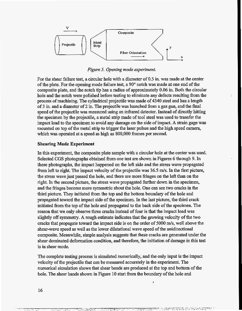
Figure 5. Opening mode experiment.

For the shear failure test, a circular hole with a diameter of 0.5 in. was made at the center of the plate. For the opening mode failure test, a 90" notch was made at one end of the composite plate, and the notch tip has a radius of approximately 0.06 in. Both the circular hole and the notch were polished before testing to eliminate any defects resulting from the process of machining. The cylindrical projectile was made of 4340 steel and has a length of 3 in. and a diameter of 2 in. The projectile was launched from a gas gun, and the final speed of the projectile was measured using an infrared detector. Instead of directly hitting the specimen by the projectile, a metal strip made of tool steel was used to transfer the impact load to the specimen to avoid any damage on the side of impact. A strain gage was mounted on top of the metal strip to trigger the laser pulses and the high speed camera, which was operated at a speed as high as 800,000 frames per second.

Shearing Mode Experiment

In this experiment, the composite plate sample with a circular hole at the center was used. Selected CGS photographs obtained from one test are shown in Figures 6 through 9. In these photographs, the impact happened on the left side and the stress wave propagated from left to right. The impact velocity of the projectile was 36.5 d s . In the first picture, the stress wave just passed the hole, and there are more fringes on the left than on the right. In the second picture, the stress wave propagated further down in the specimen, and the fhnges become more symmetric about the hole. One can see two cracks in the third picture. They initiated from the top and the bottom boundary of the hole and propagated toward the impact side of the specimen. In the last picture, the third crack initiated from the top of the hole and propagated to the back side of the specimen. The reason that we only observe three cracks instead of four is that the impact load was slightly off symmetry. A rough estimate indicates that the growing velocity of the two cracks that propagate toward the impact side is on the order of 5000 d s , well above the shear-wave speed as well as the lower dilatational wave speed of the unidirectional composite. Meanwhile, simple analysis suggests that these cracks are generated under the shear dominated deformation condition, and therefore, the initiation of damage in this test is in shear mode.

The complete testing process is simulated numerically, and the only input is the impact velocity of the projectile that can be measured accurately in the experiment. The numerical simulation shows that shear bands are produced at the top and bottom of the hole. The shear bands shown in Figure 10 start from the boundary of the hole and

16

propagate toward both sides of the sample. When the stress wave reaches the circular hole, part of it continuously propagates toward the back side of the sample and part of it is reflected by the boundary of the hole. As a result of the highly anisotropic nature of the composite, intense particle velocity gradient is generated surrounding the hole that triggers the shear bands. The particle velocity distribution around the hole is shown in Figure 11 , and the resulting shear bands are shown in Figure 10. The fracture pattern shown in Figure 9 is in good comparison with the state of in plane shear fiber matrix debonding shown in Figure 12. Thus, crack initiation moment can be predicted from the simulation.

Figure 6. CGSphoto I . Figure 7. CGSphoto 2.

Figure 8. CGSphoto 3. Figure 9. CGSphoto 4.

17

18

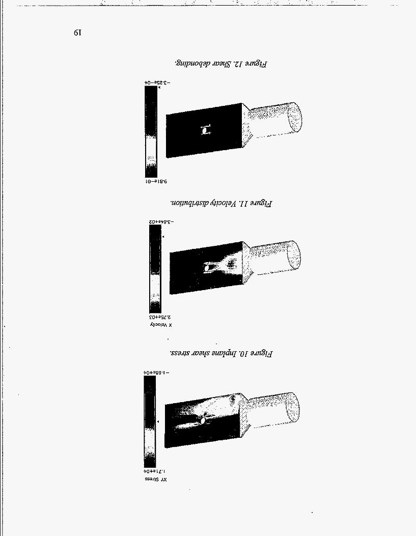
Plate Impact, Normal Failure

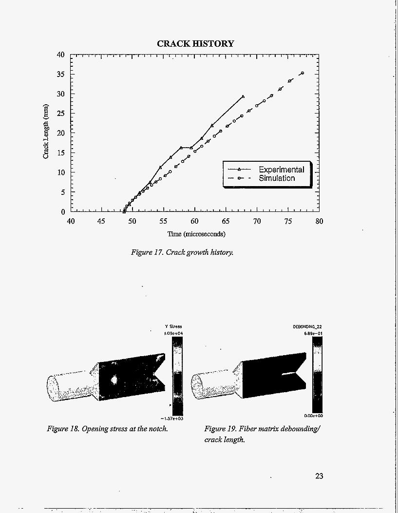
This experiment used the composite plate with a V-notch at one end. This particular sample design was obtained through numerical simulation' to eliminate the appearance of intense particle velocity gradient as we observed in the shearing mode experiments. As a result, the initiation and propagation of the damage and cracks are controlled by the opening deformation. Once again, selected CGS photographs obtained fiom one of such tests are shown in Figures 13 through 16, where the projectile impact velocity is 34.1 d s . From the first picture, one can see that as a result of the interaction of the stress wave and the notch, stress concentration was established around the tip but has not initiated a crack yet. In the next three pictures, one can observe that a crack initiates at the tip of the notch and propagates toward the impact side of the sample. Careful examination reveals that crack closure also happened behind the moving crack tip. The position of the crack tip at each moment can be obtained fiom the CGS i3nge patterns, and the whole crack propagation history is shown in Figure 17. The average crack-growing velocity is about 1700 dsec .

Similar to what we have done in the shearing mode experiment, the whole testing process was simulated numerically with the material model built into the finite element code. Figure 18 shows the state of stress at the notch sufficient to initiate the crack. According to the material model, new surface will be generated as the opening stress drops to zero. This indicates that at the moment that the opening stress drops to zero, the crack tip arrives at that element. Therefore, the crack-growing history can be extracted from the simulation, and it is compared with experimental measurement for the initial stage of crack growth in Figure 17. The material model can capture not only the initiation moment of crack growth but the growing history of the crack. Figure 19 shows the state of fiber matrix debonding or the length of the crack.

ACKNOWLEDGMENTS

The authors wish to acknowledge the valuable theoretical contributions of Frank L. Addessio and Todd 0. Williams in LANL/T-3.

Figure 13. CGS Photo I . Figure 14. CGS Photo 2.

Figure 15. CGS Photo 3. Figure 16. CGS Photo 4.

40

35

30

10

5

0 40 45 50 55 60 65 70 75 80

Time (microseconds)

Figure 17. Crack growth history.

Y stress DEBONDING-22

1.09e+04 6.89t-01

O.OOe+OO - I .57e+03

Figure 18. Opening stress at the notch. Figure 19. Fiber matrix debomding/ crack length.

23

REFERENCES

1. Aboudi, .I Mechanics of Composite Materials, A Unified Micromechanical Approach, (Elsevier, Amsterdam, Netherlands, 1991).

2. Liu, C., Y. Huang, M. L. Lovato, and M. G. Stout, “Measurement of the Fracture Toughness of a Fiber-Reinforced Composite Using the Brazilian Disk Sample Geometry,” Los Alamos National Laboratory document LA-UR-96-3845, 1996.

3. Addessio, F. L., and J. B. Aidun, “Analysis of Shock-Induced Damage in Fiber Reinforced Composites,” in High-pressure Shock Compression of Solids, Vol. 3, 1996.

4. Scott G. Bardenhagen, Michael G. Stout, and George T. Gray, “Three-Dimensional Finite Deformation Viscoplastic Constitutive Models For Polymeric Materials,” Los Alamos National Laboratory document LA-UR-96748, 1996.

5. “DYNA3D Users Manual,” Livermore National Laboratory document UCRL-MA- 107254,1993.

6 . Liu, C., A. J. Rosakis, R. W. Ellis, and M. G. Stout, “Study the Fracture Behavior of Unidirectional Fiber Reinforced Composites Using Optical Coherent Gradient Sensor (CGS) Methods,” submitted to the International Journal of Fracture, 1997.

7. Rosakis, A. J., “Two Optical Techniques Sensitive to Gradients of Optical Path Difference: The Method of Caustics and the Coherent Gradient Sensor (CGS),” in Experimental Techniques in Fracture, Ed. J. Epstein, (VCH Publishers Inc., Vo1.3, Chapter 10, pp. 327-425.

8. Haberman, K, S., C. Liu, and M. G. Stout, private communication, Los Alamos National Laboratory, 1996.