year 1 physics/astrophysics laboratory

SCHOOL OF CHEMICAL AND PHYSICAL SCIENCES

Year 1 Physics/Astrophysics Laboratory

Computer Programming with Python

A. Mahendrasingam and D.E. McLaughlin

Physics/Astrophysics

Lennard Jones Building

Year 1 Computing Lab Manual

Student Name……………………………...………………..

Keele University Physics/Astrophysics Laboratory Programming with Python Page 1

Contents

INTRODUCTION .............................................................................. 2 PYTHON: WORKSHEET 1 ............................................................... 7

Problem 1.1 .............................................................................................. 12 Problem 1.2 .............................................................................................. 14

PYTHON: WORKSHEET 2 ............................................................ 17 Problem 2.1 .............................................................................................. 19 Problem 2.2 .............................................................................................. 21


PYTHON: WORKSHEET 4 ............................................................ 30 Problem 4.1 .............................................................................................. 36



INTRODUCTION

This series of labs is meant to give you an introduction to the basics of scientific programming,

using the Python language. Python is relatively quick-to-learn and easy-to-use, and yet still fairly

powerful. It is a somewhat “new” language (first released in 1991), but it has grown rapidly and it is

finding wider and wider application in industry and in academia. It is open source, freely available

and well-documented (see www.python.org), and it can be run on any standard platform

(Windows, Mac, Linux/Unix). Advanced, scientific calculations, simulations and other applications

are still generally done using other high-level languages (e.g., Fortran, C or C++), which are older

and more established, have less frequent updates to the core standards, and also have numerous

and varied extensions (libraries) that provide for flexibility and customisation and the modification

of “legacy” programs. Moreover, Python codes execute more slowly in general than equivalent

codes written in these other languages, because Python programs are interpreted by a computer

at the time they are run, rather than being compiled into machine-language versions first. On the

other hand, compiled languages often have more rigidly structured programming rules and

apparently more idiosyncratic syntax than Python has. Writing in Python is about as close as

modern computer programming comes to writing in English. This makes Python an ideal language

in which to focus on learning and testing the ideas behind some basic procedures and methods, or

algorithms, which are generically useful for solving problems in physics and mathematics.

GETTING STARTED: BASIC TOOLS

The version of Python that you will use to do the exercises in these labs is Python 3.5. It is already

installed on the Windows machines in the large Faculty of Science PC Lab in the Lennard-Jone

Building (LJ 0.26) and in the smaller Physics and Astrophysics PC Lab in Lennard-Jones (LJ

1.27).

To start up Python 3.5 on a machine in LJ 0.26, go into the Physics folder on your Desktop

and double-click on the shortcut called python 3.5. This opens an interactive IDLE shell, or

window. IDLE is Python’s built-in Integrated Development Environment and is what you will be

using to complete all of the work in these labs: testing and de-bugging bits of code in real time,

and writing, saving and running complete programs. If you wish to run Python under Windows

in LJ 1.27, look instead in the Start Menu for a folder called Python 3.5 (it should be listed

under “All Programs”). Inside this folder is a shortcut called IDLE (Python GUI) and double-

clicking this will open an interactive IDLE shell.

http://www.python.org/


All of the executables, libraries and dll files, etc. for the Windows installation of Python 3.5 are

stored in the folder C:/Python35. You should not have to go to this folder just to start up IDLE or

another Python executable, and you should not open directly any of the other files associated with

the installation. However, you need to be aware that the C:/Python35 folder will (at least initially)

be the default location where Windows tries to store the programs that you write and save to disk

from inside IDLE. But you should never save any material whatsoever in the C:/Python35 folder. When you come to save programs that you have written, or when you open and run

programs that you saved previously, go instead to a location that you decide on your S: drive.

To get a flavour of the Python language and working in the IDLE environment, and (crucially!) to

see how to save complete programs and run them later either from within IDLE or outside it, work

carefully through the rest of this Introduction before you move on to any of the subsequent

Worksheets. Here, and throughout, pay close attention to exactly what you type. Python is

case-sensitive and so (for example) recognises a command such as “print”, but not “Print” or

“PRINT”. Also, quotation marks and spaces can have very specific meanings, and leaving some

out or inserting extra ones may have unintended consequences.

You can always access the full, offline documentation for your version of Python, including

detailed Table of Contents and Index and Search capabilities, by selecting “Python Docs” from

under the “Help” tab that is found along the top of any IDLE shell. A useful tutorial is also available

within this documentation, along with much more advanced help and advice. Documentation and

tutorials are also available online, at www.python.org, but these may be for versions of the

language other than the one installed on your computer.

THE IDLE SHELL AND A SIMPLE FIRST PROGRAM

Start IDLE using the appropriate shortcut as described above. A window (or shell) will appear that

is mostly empty, with your cursor beside a command-line prompt of three greater-than signs (>>>)

near the top. At the prompt, type

print("Hello.")

and press the <Enter> key. Here print() is an example of a built-in function in Python: the word

actually invokes a piece of code “under the hood” of the language, which takes a specific

argument (everything in parentheses after the function name—in this case, “Hello.”) and performs

a well-defined action upon it. In this case, obviously, the action is just to print the argument to the

http://www.python.org/


IDLE screen. Note that the quotation marks around the word “Hello” do not get printed out,

however. They are there to identify just what is supposed to be printed. (Technically, quotation

marks identify any sequence of characters between them as a string constant or literal.) Try typing

print(Hello.) without the quotation marks to see an example of a syntax error.

The names, actions and syntaxes of built-in functions in Python can be looked up in the Python

Manual accessed through the Help tab (i.e., “Help > Python Docs”) in the menu at the top of the

IDLE window.

Now, with your cursor at the prompt on the next free line in IDLE, type

name= input("What is your name? ")

and press <Enter>. You will see the cursor flashing just after the question mark asking for your

name. This means that the program is now waiting for input, so type in your name and press

<Enter> again. This returns you to the IDLE command prompt (>>>) and frees up the terminal for

further commands.

Here, input is another built-in function. This one takes an argument (“What is your name? ”), prints

that to the screen, and then waits for input directly from the user. Everything typed by the user,

until <Enter> is pressed again, is taken by the function and stored in memory as the value of a

string variable that is called (in this example) name. After the user has pressed <Enter> to

complete the input, nothing more is done with the input, unless and until the variable is referred to

in later statements or commands. In principle, almost any word (excepting only those that already

refer to built-in functions) can be used to refer to a variable—this one did not have to be called

name—but it is good practice to choose words that have fairly obvious meanings and are likely to

make sense both to you and to any other readers or users of your code. (Again, Python is case-

sensitive; so, for example, a variable called name is distinct from one called Name.)

Finally, type

print("Goodbye " + name + ".")

and press <Enter>. Now the argument to the built-in print() function is the concatenation of two

separate string constants (each contained in quotation marks) on either side of the value of the

variable name (written without quotation marks) that you entered just above. The plus-signs inside

the parentheses join the constants and the (value of the) variable together into a single string for

printing.


You should now have some feel for working in the IDLE shell. One thing you will have noticed, as

you were entering the few lines of code above, is that various words appear in different colours.

This is done in order to distinguish explicitly between (for example) built-in functions, constants,

variables and other fundamental elements of the language. These visual distinctions can be very

helpful when you’re trying to build up a real code without mistakes, and/or to identify problems of

logic or syntax in an existing program. The colouring follows a pre-defined default scheme. You

can see the details by clicking on “Options > Configure IDLE > Highlighting” in the menu at the top

of the IDLE window. (Exit this menu item by clicking “Cancel” rather than “Ok” or “Apply” if you

don’t want to change the defaults.)

You should also try moving your cursor around inside the IDLE shell, using the mouse and the

arrow keys, to see how you can repeat and/or edit commands that were entered previously.

SAVING AND RUNNING PROGRAMS

Technically, the three Python lines (or statements) that you entered into IDLE above constitute a

program. But no program is particularly useful until it has been stored in a file on disk that can be

run (and/or edited, expanded, etc.) at will, at any later time.

IDLE gives you access to the interactive mode of Python, which you can use to try out short

ideas and get immediate feedback, quickly check that the results are what you expect, see

warnings about syntax errors, and so on. To save a program that can be run later, independently

of anything else you do in IDLE, you need to work in script mode, which requires opening a

different shell or window. You can do this from within IDLE and then have both shells open at

once, using the interactive shell to try things out and the scripting shell to contain the final code

that will be saved to disk.

Go to the “File” menu at the top of the interactive IDLE shell, and select “New Window”. A

completely empty shell will appear that looks nearly the same as your interactive one, except it

doesn’t have a command prompt (>>>) in it, and the menu items across the top include “Format”

and “Run” tabs rather than the “Shell” and “Debug” menu tabs that are in the interactive shell. This

new window is your scripting shell. Type the following program into it:

print("\n" + "Hello.") name=input("What is your name? ") print("Goodbye " + name + ".") stop=input("\n" + "Press <Enter> to quit. " + "\n")


There are some minor new elements in this program. One is the presence of “\n” at a few places

inside the arguments to one of the print() statements and one of the input() statements. Each

instance of “\n” represents an instruction to print an entirely blank line to the screen, just to make

the output of the code look cleaner and easier to read (the n is for “new” line; the \ makes the n be

interpreted in this way rather than printed literally as a letter of the alphabet). Second, the final line

of the program is present simply to force the program to “hang” after doing its main work, and wait

until the user physically hits <Enter> before it finishes completely. This is done in order to prevent

programs exiting and closing windows too rapidly (before output can be read!) when they are run

outside of IDLE. Finally, the last line of the program is set off from the others by a blank line before

it. This is not required for any reason by Python; but it is not disallowed, either, and leaving some

lines intentionally blank like this can help to organise a code and make it more readable.

Now that the program has been written in the scripting shell, it can be saved. Go to the “File” menu

tab at the top of the scripting shell, left-click on it and select “Save As…”. A window will come up,

which you can use to navigate to any folder you like to save your work, and to give a name to the

saved program file. Python’s initial default option for the save folder is C:/Python35 but again: you

should not save your work in this folder. Navigate instead to some location on your S: drive and

keep your programs there. (Just be sure you remember where it is!) The name of the program file

can be anything you choose, but it must end in the extension .py and you will need to type this

extension explicitly as part of the filename. A saved program can then be run in either of two ways.

To run a saved program within IDLE: If the program is already open in a scripting shell, simply

choose “Run > Run Module” from the menu options at the top of the scripting shell. The output

from the code will appear in an interactive IDLE shell, which is also where you can enter any input

that the program asks for. If an interactive IDLE shell is open but no scripting shell is open, choose

“File > Open” from the IDLE menu options and navigate to the location of the saved program on

your S: drive. The program will then open in a new scripting shell with a Run tab in its top menu.

To run a saved program directly from Windows, bypassing IDLE and scripting shells altogether: Go to the folder on your S: drive that contains the program file and double-click the file

name (which, again, must end in the extension .py). A DOS window (CMD Prompt) will be

opened to display the program output and to accept any input that the program wants. This

window will be closed instantly when the last statement of the program has been executed (hence

the need for the final “hang” line that you wrote above).

Try both of these methods of running your saved program and make sure that both work perfectly

for you before you proceed to Worksheet 1.


PYTHON: WORKSHEET 1 Open an interactive IDLE shell and a new scripting window. Type the following program into the

scripting window exactly as it is written here:

# Program to solve a quadratic equation, ax^2 + bx + c = 0 import cmath # functions in the cmath module work with complex numbers a = input(" Please enter the number a: ") b = input(" Please enter the number b: ") c = input(" Please enter the number c: ") # a=float(a) b=float(b) c=float(c) # disc = b**2 - 4*a*c disc = cmath.sqrt(1.0*disc) x1 = (-b + disc)/(2.0*a) x2 = (-b - disc)/(2.0*a) print("\n" + "Solutions are: x = " + str(x1) + " and x = " + str(x2)) stop=input("\n" + "Press <Enter> to quit." + "\n")

In order to write a computer program such as this, one has to break down the method of solution

of a problem into a series of sequential steps. This is called an algorithm. It is important to follow

through this program line-by-line to make sure you understand how it solves the quadratic-

equation problem within Python.

First, anything written following a hash (#) on a line does not form part of any statement or

command on the rest of the line and is not executed as code; instead, it is treated as a comment

and is ignored by the Python interpreter. You may (should!) put comments liberally in your

programs to help yourself and others understand them.

Second, at the top of the program is the statement import cmath. The word import tells Python

that the program is going to make use of one or more built-in functions that are kept in a particular

collection of related functions (known as a module), which, while standard to the language, are not

made available automatically to all new programs but have to be explicitly “loaded in” to them. In

this case, the module needed is cmath, which includes a number of mathematical functions for

operations with complex numbers. You can read about this module in the Python Manual,

available through “Help > Python Docs” in the IDLE menu. The function from cmath that is needed


in the program above is the square-root function, sqrt(). Note that the only reason for importing

the cmath module—as opposed to the math module, which contains the square-root and other

functions for operating on real numbers—is the possibility that the discriminant of a quadratic

equation may be negative, and its square root imaginary.

Following the import statement is a statement that invokes the built-in function input(), which is

not actually part of cmath but is always available to any program, no matter what other modules

have or have not been imported. Note that, as written here, the input() statement is asking for

numerical value to be entered and values that will be stored in the variables called a, b and c.

The concept of a variable is a very important one. In the program above, the quantities a, b, c, disc, x1 and x2 are numerical variables. Think of the memory of the computer as a series of

boxes, each of which can contain one piece of data. Whenever you introduce a new variable name

in a program, it will be attached to one box in memory, and thereafter in the program the variable

name will refer to the value (whether a number or a string) stored in that box. As mentioned

before, variable names can be almost anything you like, as long as they start with an alphabetic

character and do not take the name of any built-in function. Always try and give variables

meaningful names.

Variables can be used together with constants and operators to make expressions. An example

of a numerical expression in the above program is b**2 - 4*a*c. (There are also several string

expressions, in the arguments to the input() and print() functions.) When Python encounters an

expression involving variables, it works out its value using the current values of the variables. The

mathematical operators for numerical variables are +, −, * (multiply), / (divide) and ** (raise to

the power). Python obeys the usual order of operations, and brackets can always be used to make

the mathematical meaning of any expression unambiguous. For string variables and constants, an

important operator is + (concatenation), which we have already encountered.

Statements such as a,b,c = input(…) or disc = b**2 - 4*a*c assign the values of expressions to

variables. This means the expression (or function) on the right-hand side of an equals sign is

evaluated (or performed), and the result is put into the memory referenced by the variable(s) on

the left-hand side. This creates the variables if they hadn’t been referred to previously in a

program, or it gives them new values if they had been assigned values earlier in the program.

The final unfamiliar pieces of syntax in this program involve the built-in functions cmath.sqrt() and

str(). It should be clear what the function sqrt() refers to; the cmath joined to the front of this by a

dot is simply identifying the module (imported in the first line of the program) that contains the

sqrt() function. The str() function—which, like print() and input(), is always available and doesn’t


require any modules to be imported—converts numerical values (including complex numbers) into

strings, which is done here with x1 and x2 inside the argument to the print() function.

Save your quadratic-equation program to a file with a meaningful name (ending in .py) in the

location you have chosen on your S: drive, and run it in IDLE to see how it works. (Note that if you

edit a program in the scripting window and then select “Run > Run Module” from the window menu

before saving the changes, you should be prompted to save the file first.) Think up test cases:

quadratic equations, ax2 + bx + c = 0 with particular values of a, b and c, whose roots you know.

Pick cases with both real and complex roots, and see if your program gives the right answers.

The arguments of functions can be entire expressions, as well as variable names. Use this fact to

modify the program above, eliminating its third statement (not counting comments). Check that the

program still works properly.

CONSTANTS, VARIABLES AND EXPRESSIONS Type the following statements one by one into an interactive IDLE shell. There is no need to enter

them into a scripting shell to be saved as a program; just make sure that you understand how

Python evaluates each expression, and what point is being is being made in each case.

print(6+10/2) print((6+10)/2) print(2.5/1.0e12) print(12/6*2) print(12/(6*2)) print(1.0e3) print(27**113)

Next, try the following set of statements:

a = 4 print("a+5") print(a+5) a = a+5 print(a+5)

Then, pay close attention to the results of each of the following: print(2/3) print(2.0/3.0) a=2.0/3.0 b=2/3 print(a*b) print((2.0/3.0)*2/3) print(1/a) print(1/(2/3))


In Python (or, in fact, in any other scientific programming language), there is a fundamental

difference between expressions like 2.0/3.0 and those like 2/3. It is crucial that you understand

exactly what the difference is and can explain the results of each of the print() statements just

above… so make sure that you do (i.e., ask if you don’t).

Finally, to remind yourself of the difference between string constants and variables:

Hello = "Goodbye" print("Hello") print(Hello)

BUILT-IN FUNCTIONS There are many functions built into Python that can be used in expressions. As already seen

above, some built-in functions — like print(), input() and str() — are always available and can be

used in any program without any further thought; while others — such as sqrt() — are only

included in collections of related functions, or modules, that must be imported explicitly into a

program before the function can be used. You can get an overview of the “always-available” built-

in functions and the various functions in modules that need importing, from the Python

documentation: Select “Help > Python Docs” in the IDLE menu. In the Documentation that comes

up, click through to the Library Reference and go to Section 2 there.

Not surprisingly, one module that you will frequently need to import into your programs is the math

module, which includes a large number of functions for operations involving real numbers (that is,

the arguments to these functions must be numerical variables, constants or expressions with real

values; they cannot be complex). The functions in this module are listed and described in detail

under Section 9.2 of the standard Library Reference in the Python Documentation.

Below are several one-line examples using functions from the math module. Try each of these in

the interactive IDLE shell to see what it does, and read more about the functions in the

Documentation if anything is unclear. You may want to make notes for yourself of what does what

in the following, and you may also want to put these lines into a program that you can save and

run later, for reference.

First, whether in IDLE or in a scripting window for a program to be saved, you need to type

import math

Then try the following:


pi = 3.1416 print(pi) print(math.pi) print(int(math.pi)) print(math.sin(pi/6)) print(math.sin(pi/6)**2 + math.cos(pi/6)**2) angle = math.atan(1.0) print(180.0*angle/math.pi) print(math.degrees(angle)) angle = 45.0 print(math.radians(angle)) print(math.e) print(math.e**(2.0)) print(math.exp(2.0)) print(math.log(7.389)) print(math.log10(7.389)) print(math.sqrt(4.0)) print(math.sqrt(-4.0)) print(math.fabs(-7.7)) print(math.fabs(7.7)) print(math.factorial(3.0)) print(math.factorial(3)) print(math.factorial(3.1)) print(int(7.7)) print(int(7.7+0.5)) print(math.trunc(7.7)) print(math.trunc(7.7+0.5)) print(int(-5.0/3.0)) print(int(-5/3))

In the above, every built-in function that is referenced with “math.” in front of the function name is

found only in the math module and will not be available to any program unless the statement

import math appears before the function is invoked. The built-in function int() is used often

enough that it is actually outside the math module and is one of those that is always available to

any program, without any importing. (What does int() do?)

Also, in the above, pi, angle, a and b are variables. The quantities math.pi and math.e may look

at first glance like built-in functions in the math module, but in fact they are built-in constants, with

“exact” values of π and e stored to the limits of machine precision. Actually, you can tell that these

are not functions by the lack of parentheses () immediately after their names: math.pi and math.e

do not take arguments like functions do.


Now that you have experience with some key basics of Python and the use of built-in

mathematical functions, you can write a program to solve the following simple physics problem.

You will need to import math near the beginning of the program, and don’t forget to type

everything in a scripting window so you can save the final program to your S: drive and run it later.

Use comments liberally in your program to help you remember (and explain to others) the logic

behind your algorithm, the meanings of your variable names, and so on.

LOGICAL EXPRESSIONS Logical expressions test relationships between numerical or string variables or expressions and

evaluate to either True or False. They are formed using the following relational operators:

> (greater than) < (less than) >= (greater than or equal to) <= (less than or equal to) == (equal to) != (not equal to)

With strings, “greater than” and “less than” refer to alphabetical order. Logical expressions may be

joined with and and or, or negated with not. To see how these work, type the following in IDLE:

print( 7 > 6 ) print( 6 >=7 ) print( "seven" > "six" ) print ("seven" <= "six") print( 2+2 == 4 ) print( 3+3 > 7 ) print( (2+2 == 4) or (3+3 > 7) ) print( (2+2 == 4) and (3+3 > 7) ) print( (2+2 == 4) and (not (3+3 > 7)) )

Problem 1.1

If a projectile is fired with speed v from the ground at an angle θ to the horizontal, the

horizontal distance (range) it travels is given by R = (v2/g) sin(2θ), where g is the

acceleration due to gravity.

Write a program that will take the values of θ (assumed to be in degrees) and v (assumed

to be in m/s) as user inputs, and print out the range R in metres. (You can set the

constant g=9.81 m s−2 inside the program.) Use your program to investigate how R varies

with θ for a fixed value of v. At a given v, for what value of θ is R a maximum?


DECISIONS: if…else Get back the quadratic-equation program that you wrote and saved earlier (page 7). Run it again

to see what happens when you input values of the variables a, b and c that give two real roots for

x, versus complex roots (for example, try a, b, c = 1, 4, 2 versus a, b, c = 1, 2, 3).

That program is able to handle the case of complex roots because it imports the module cmath,

which contains built-in functions that are designed to work with complex numbers. However, it is

important to have some idea of how the functions in cmath deal with complex numbers.

Therefore, change the statement import cmath at the top of the program to import math instead,

so that you are forcing yourself to use built-in functions that can only work with real numbers

(either as arguments or as results). You then must also change the occurrence of the built-in

function cmath.sqrt() to math.sqrt() instead. Save the revised program (under a different name…

i.e., after editing the program in a scripting window, select the menu option “File > Save As…” to

save it.) Now what happens if you try to solve a quadratic equation that does not have real roots?

To get around this problem while still using only real numbers, and functions only from the math

module (not cmath), modify your program so it appears exactly as follows:

# Program to solve a quadratic equation, ax^2 + bx + c = 0, with real roots import math # functions in the math module only work with real numbers a = input(" Please enter the number a: ") b = input(" Please enter the number b: ") c = input(" Please enter the number c: ") # a=float(a) b=float(b) c=float(c) disc = b**2 - 4*a*c if (disc >= 0): disc = math.sqrt(1.0*disc) x1 = (-b+disc)/(2.0*a) x2 = (-b-disc)/(2.0*a) print("\n" + "Solutions are: x = " + str(x1) + " and x = " + str(x2)) else: print("\n" + "Error. No real roots.") stop=input("\n" + "Press <Enter> to quit." + "\n")

Now try running it again with a set of a, b, c values that lead to complex roots. This is still not

entirely satisfactory, but at least the program doesn’t crash. On the other hand, try giving an input


value of a=0 to this program, along with any values at all of b and c. What happens in this case?

This needs to be fixed.

In the absence of any control structures, a program runs by starting at the first statement and

executing the following statements one-by-one until the end is reached. We have just seen an

example of a control structure, if…else. Inside parentheses following the word if is a logical

expression, disc >= 0, which evaluates to either True or False. If the result is True, then the

program executes the block of statements that immediately follow the if statement and are

indented by a fixed number of spaces from the beginning of the line. In this case, the else

statement and any block of uniformly indented statements immediately following it are ignored

altogether, and the program continues with the first unindented statement it finds after the else branch of the structure. If the logical expression in the if statement is False, then instead the

whole (indented) if branch of the structure is ignored, the statements indented after the else

statement are executed instead, and once those are done the program then continues on from

where the indenting stops. (The else branch may be omitted if it is not required, i.e., if you don’t

actually want to do anything special at all in the case that a particular logical expression is false.)

In Python, for an if…else control structure to work properly, the statements actually containing the

words if and else must not be indented; while the blocks of statements to actually be executed in

each of the two branches must be indented, and all by the same number of spaces. It is only

when this indenting stops that Python knows it is out of one if…else branch and into the next, or

out of the entire structure altogether and back to sequential statements that are executed in all

cases. When writing code in IDLE or in the associated scripting shell, the commands on lines

following if and else statements will be automatically indented for you, by a default, fixed number

of spaces. You need to stop this indentation yourself (backspace to delete the leading spaces that

automatically appear on a line) when you decide that any part of an if…else structure is complete.

Problem 1.2

Modify the program on page 13 so that it prints out the roots in the case where they are

complex. Use only built-in functions from the math module; do not import cmath. Since

the functions in math can only operate on real numbers, you will need to handle the real

and imaginary parts of complex roots separately.

Also, use another if…else control structure in this program to make it handle the case

a=0 correctly without crashing.

Test the final version of the new code thoroughly, and save it to your S: drive.


LOOPS: for AND WHILE Another important control structure is the for loop. Try this program: # Program containing a for loop import math print("\n" + "Table of square roots" + "\n") for i in range(1, 10, 1): print(str(i) + " " + str(math.sqrt(1.0*i))) stop=input("\n" + "Press <Enter> to quit." + "\n")

The for loop here executes a block of statements repeatedly for successive values of the variable

i determined by the three arguments given to the built-in range() function. (This is another function

that is automatically available to all programs and does not require any module to be imported.)

The block of statements to be executed repeatedly as part of a loop are indented, by the same

number of spaces, exactly as for the branches of an if…else structure. The end of the block of

statements to be looped over, and a return to sequential statement execution (after the full range

of i has been gone through), is indicated by stopping the indentation. (In the small example here,

the “block” is just a single print(…) statement.)

Experiment with the arguments to range() in the program just above, to see what they all mean. In

particular, figure out how to change the step size between successive values of the loop variable i. Then modify the program so it uses a for loop to print a table of cube roots for all the odd integers

only between 1 and 11, including both 1 and 11. If you use the fact that the cube root is the 1/3

power of a number, then you need to remember that there is a difference between the quotients

(1/3) and (1.0/3.0) in Python.

In working some of these things out, you may find it helpful to look at another example as well:

# Another program with a for loop import math for degrees in range (0, 95, 5): radians = math.pi*degrees/180.0 print(str(degrees) + " " + str(radians) + " " + str(math.sin(radians))) stop=input("\n" + "Press <Enter> to quit." + "\n")

The for loop repeats a block of (properly indented) commands a specific, pre-determined number

of times. We can also have loops that repeat an initially undetermined number of times (even,


potentially, either indefinitely or not at all) depending on whether a logical expression evaluates as

true or false. This kind of repetition is done using a while loop. One case you might imagine,

which requires a while loop, is asking a user for some input and continuing to ask until the input

entered is equal to some particular, desired value. Here is an example of this:

# Program illustrating the use of a while loop name = "none" while ( (name != "stop") and (name != "STOP") ): name = input("What is your name? ") print ("Hello " + name + ".") stop=input("\n" + "Press <Enter> to quit." + "\n")

Again, the program starts to execute statements sequentially, so the first thing it does is assign the

value “none” to a string variable called name. It then comes to the while statement, which tests to

make sure that the value of name is not equal to either “stop” or “STOP”. If it is not, then the block

of uniformly indented statements immediately after the while are executed—the user is asked to

input a new value for name, and then the program says hello—until the program encounters the

first unindented line (blank lines are always overlooked). It doesn’t execute the unindented line

(yet) but loops back to the while statement to test whether the new value of name is either “stop”

or “STOP”. When the user finally enters one of these words as name, the logical expression in the

while statement will be false the next time it is executed. Then the program will stop looping, skip

over the indented statements in the while block, and resume simple, sequential execution of the

rest of the code from the first unindented line that follows. (In this example, the “rest of the code” is

just our usual, one-line “hang” waiting to exit entirely.)

Actually, the program above does not quit in the most sensible way when it is finally given stop (or

STOP) as an input for name. We can take care of this by subtly changing the order of asking the

user for a name and testing that name in the while statement, and by exploiting the fact that

Python allows for while loops to contain else branches (as the if…else structure and, in fact, the

for loop also allow). Thus, try the next program now. Be sure you understand fully the different

behaviour when the loop is terminated in this program versus the previous one.

# Program illustrating the use of a while…else loop

name=input("What is your name? ") while ( (name != "stop") and (name != "STOP") ): print ("Hello " + name + ".") name=input("What is your name? ") else: print("Fine. Don’t tell me. ")

stop=input("\n" + "Press <Enter> to quit." + "\n")


PYTHON: WORKSHEET 2

Statistics and random numbers are important tools in computational physics and astrophysics,

with applications ranging from straightforward data analysis to the numerical approximation of

ideal mathematical expressions and the simulation of extremely complex physical systems. In this

Worksheet, you will generate sets of (pseudo)random numbers and develop algorithms using

them to compute basic statistics (mean and standard deviation) and to estimate the value of π.

First, we need to set out how to keep track of a running sum of a set of numbers. Thus, try the

following, which simply adds all the integers from 1 through 20:

# Algorithm for the running sum of a set of integers thesum = 0 for i in range(1, 21, 1): thesum = thesum + i print("The sum of integers from i=1 to i=" + str(i) + " is: " + str(thesum)) stop=input("\n" + "Press <Enter> to quit." + "\n")

Note a few important things here: First, we are storing the sum of the integers in a variable called

thesum. You might be tempted to call this variable just “sum”, but there is actually a built-in

function in Python called sum() — which we can’t use in this program, because it does not do

quite what we want — and it is good practice in general to avoid possible confusion between your

own variable names and built-in elements of Python itself. Second, the program starts by setting

thesum=0. This initialises the variable. It is good practice always to explicitly assign a value to any

variable you want to have in a program, before you start using the variable in expressions or

modifying it in any way. Third, the built-in range() function, which you encountered already in

Worksheet 1, takes 21=20+1 as its second argument in order to make the counter variable i in the

for loop go up to and include the desired maximum of 20.

Next, let us see how to generate “random” numbers. There are many built-in functions in Python

for working with random numbers. All of them are stored in the random module, which is

described in detail in Section 9.6 of the standard Library Reference in the Python Documentation.

Thus, we need to import random into any programs where we want to use random numbers.

(This module is distinct from the math module, so very often we still need to import math as well.)

With this in mind, the following short program will generate some user-specified quantity num of

random numbers x — all having values 0 ≤ x < 1 — and also calculate the mean of these

numbers:


# Program to generate random numbers and calculate their mean import random num = input("\n" + "How many numbers do you want to generate? ") num = int(num) random.seed() thesum = 0.0 for i in range(1, int(num)+1, 1): x = random.random() thesum = thesum + x mean = thesum/(1.0*num) print("The mean of your numbers is: " + str(mean)) stop=input("\n" + "Press <Enter> to quit." + "\n")

This program makes use of two of the built-in functions in the random module. The first,

random.seed(), is used to initialise the random-number generator in Python. This raises some

technical issues about exactly how “random” the numbers generated by computers really are.

Suffice it to say that they are better described as pseudo-random numbers, meaning (very

roughly) that they are generated in a deterministic (not unpredictable) way following the

specification of an initial value (the seed), which may be randomly set. The function

random.seed() specifies this seed value. If it is invoked without an argument, as in the program

just above, then Python uses the computer’s clock time to define the seed, and every time you run

the program it will generate a truly different sequence of numbers and give different results for

calculations using them. If you do give a (constant) argument to the seed function — for example,

you might write random.seed(8.7) — then every time you run the program it will generate the

same sequence of random numbers.

The function random.random() generates a single “random” number between 0 (inclusive) and 1

(exclusive). The numbers generated by this function are uniformly distributed, i.e., there is an

equal probability of any one number having any value between 0 ≤ x < 1. The random module

does contain other functions for generating numbers that fall between different limits and/or that

are distributed differently between the limits (e.g., following a Gaussian). You can learn more

about these alternatives in Section 9.6 of the Library Reference part of the Python Documentation.

Test the program above by inputting (for example) values of 1,000 then 10,000 then 1,000,000 for

the number num. Run the program several times for each value of num, to see the differences in

the means you get out each time. What do you expect the value of the mean to be in the limit of

arbitrarily large num?


Problem 2.1

The standard deviation of a set of numbers {𝑥𝑥𝑖𝑖} is defined by

𝜎𝜎 = �⟨(𝑥𝑥 − ⟨𝑥𝑥⟩)2⟩

where the notation ⟨𝐴𝐴⟩ represents the mean of all the values of quantity A.

First, show algebraically that the definition of σ can be re-written as

𝜎𝜎 = �⟨𝑥𝑥2⟩ − ⟨𝑥𝑥⟩2

This form is more appropriate for computer analysis and is the one you should use. Why?

Now modify the program above, which already calculates the mean of some user-

specified quantity of uniformly-distributed random numbers between 0 and 1, so that it will

also calculate (and print out) the standard deviation of the same set of numbers. To what values do the mean and the standard deviation tend, as you generate more and

more random numbers? Can you explain these limiting values for ⟨x⟩ and σ?

You will need to import both the math module and the random module into your new

program, which you can do with a single statement: import math, random

Include as many comments as you see fit in your program, test it thoroughly as you go,

and be sure to save it to your S: drive when it is done.

Now, do the following problem:

Now you will use pairs of uniformly-distributed random numbers between 0 and 1 to obtain an

estimate for the value of π. The idea—which is actually an example of a powerful and widely used

numerical method called Monte Carlo integration—is as follows.

Suppose we generate two random numbers, say x and y, each distributed uniformly between

0 ≤ x < 1 and 0 ≤ y <1. If these were plotted together as a coordinate in the xy plane, they would

define a point somewhere in (or on the boundary of) a square with sides of length 1. If we were to

generate arbitrarily many such pairs of numbers, then eventually the points they define would fill in

this entire square. Moreover, each uniformly-distributed (x,y) point generated in this way would

have an equal probability of falling anywhere in the square, and so eventually they would fill in the

entire area evenly, i.e., the density of points would be the same everywhere.


The square defined by 0 ≤ x < 1 and 0 ≤ y < 1 contains the (positive-x, positive-y) quadrant of a

circle of radius 1. If the area of the entire square becomes evenly filled in after randomly

generating a very large number of uniformly-distributed (x,y) points, then of course the quadrant of

the radius-1 circle inside the square also gets evenly filled in—as this figure illustrates:

In the left-hand panel here, 200 independent random numbers are put into pairs and plotted as

100 points in the xy plane; in the middle panel there are 500 randomly generated (x,y) points; in

the right-hand panel there are 2500 points. Green points have distances �x2+y2 ≤ 1 from the

origin and so fall within the positive-(x,y) quadrant of the circle with radius 1 (the dashed curve).

The area of the circular quadrant in this figure is π/4 (one-quarter the area of a circle with radius

r = 1), while the area of the full square is just 1. Thus, the ratio of the areas is π/4. But when the

square is filled in evenly, this ratio of areas must equal the ratio of the number of points inside the

circular quadrant to the total number of points in the whole square. Since the even filling happens

as the number of points increases, we conclude that: If N points (x,y) are generated randomly,

with x and y independent of each other and both distributed uniformly between 0 and 1, then in the

limit of large N, the fraction of points having r ≡ �x2+y2 ≤ 1 must tend to the value π/4.


Problem 2.2

Once you have completely understood the argument just above, calculate the value of π

by Monte Carlo integration, using the random number generator random.random().

Let the number N of (x,y) points to generate be input to the program by the user, and

make the program output (1) the value of π estimated for the input N value; (2) the “true”

value of π according to Python (i.e., the built-in constant math.pi); and (3) the

percentage relative error in your Monte Carlo estimate of π, which is defined by

100 × (your estimate – π) ÷ π.

Experiment to see how your numerical estimate for π depends on N. What N do you need

to reliably (i.e., repeatably) obtain a value for π that has a relative error of 1%? A relative

error of 0.1%? A relative error of 0.01%?


PYTHON: WORKSHEET 3 In this Worksheet, you will make use of what you have learned so far (especially about the while

loop) to investigate the problem of testing numerically for the convergence of infinite series. Then,

you will go on to learn some techniques for working with sets of numbers in Python—techniques

that would be useful, for example, in the analysis of experimental data. You will learn about data

constructs called lists (which are similar to arrays in many other languages), how to do some

basic operations on lists, and how to write to and read from files on disc (data input/output, or I/O).

SERIES Infinite series come up surprisingly often in computational problems—such as in the solutions to

the integrals of many functions, or in the evaluation of “special” functions that don’t have closed

analytical forms. They also appear in the context of evaluating functions like exp(x) or

approximating the values of constants like π. It is therefore important to be able to test for the

convergence of series, and to approximate their sums to any desired accuracy with a finite number

of operations. For example, consider the convergent series

� 1𝑘𝑘2

∞

𝑘𝑘=1

= 1

12 +

122

+ 1

32 + ⋯

The following program sums the terms in this series until the terms become less than some

(small!) value specified by a variable called tolerance. It then stops, and the sum of the finite

number of terms to that point is taken as an approximation of the series sum to infinity.

# Program to approximate the sum to infinity of terms (1/k^2) tolerance = input("\n" + "Enter a value for the tolerance: ") tolerance = float(tolerance) k = 0 thesum = 0.0 nexterm = 1.0/((k+1)*(k+1)) while (nexterm >= tolerance): k = k + 1 thesum = thesum + nexterm nexterm = 1.0/((k+1)*(k+1)) print("\n" + "Terms are below tolerance for k > " + str(k)) print("Sum of terms to k = " + str(k) + " is: " + str(thesum)) stop=input("\n" + "Press <Enter> to quit." + "\n")


Study this algorithm closely and test the program using several values for the tolerance. By

specifying smaller and smaller tolerance and noting the associated change in the value of

thesum, obtain an estimate for the sum to infinity, S∞ , that is accurate to five significant figures.

Hence, what is the value of �6S∞ ?

This basic method of convergence testing can be used to tackle the following:

LISTS So far, you have been dealing with variables that are just single numbers or strings. However,

working only with individual objects can make it slightly cumbersome to determine even simple

facts about collections of numbers, such as their sum (recall Worksheet 2), or their minimum and

maximum. Consider the following program, which keeps track of the running sum, minimum and

maximum of a set of numbers input by the user:

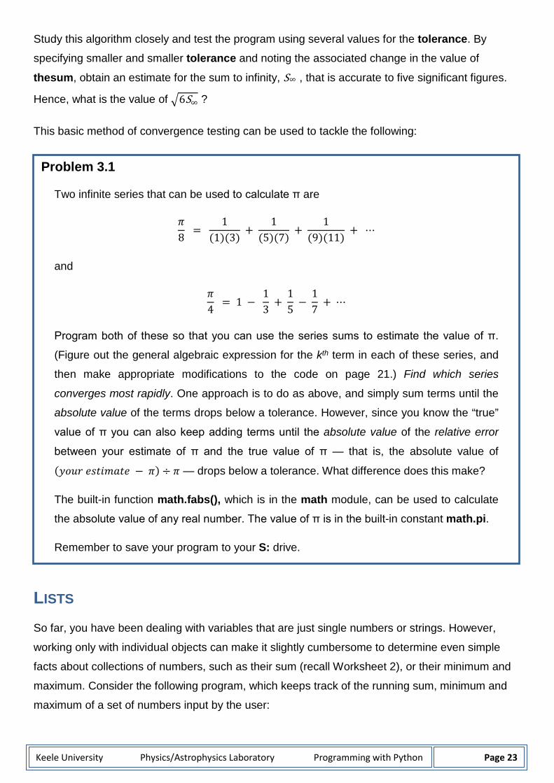
Problem 3.1

Two infinite series that can be used to calculate π are

𝜋𝜋8

= 1

(1)(3) +

1(5)(7)

+ 1

(9)(11) + ⋯

and

𝜋𝜋4

= 1 − 13

+ 15

− 17

+ ⋯

Program both of these so that you can use the series sums to estimate the value of π.

(Figure out the general algebraic expression for the kth term in each of these series, and

then make appropriate modifications to the code on page 21.) Find which series

converges most rapidly. One approach is to do as above, and simply sum terms until the

absolute value of the terms drops below a tolerance. However, since you know the “true”

value of π you can also keep adding terms until the absolute value of the relative error

between your estimate of π and the true value of π — that is, the absolute value of

(𝑦𝑦𝑦𝑦𝑦𝑦𝑦𝑦 𝑒𝑒𝑒𝑒𝑒𝑒𝑒𝑒𝑒𝑒𝑒𝑒𝑒𝑒𝑒𝑒 − 𝜋𝜋) ÷ 𝜋𝜋 — drops below a tolerance. What difference does this make?

The built-in function math.fabs(), which is in the math module, can be used to calculate

the absolute value of any real number. The value of π is in the built-in constant math.pi.

Remember to save your program to your S: drive.


# A program for the running sum, minimum and maximum of user-entered numbers num = input("\n" + "How many numbers would you like to enter? ") thesum=0.0 for i in range (1, int(num)+1, 1): x = input("\n" + "Enter a number: ") x = float(x) thesum = thesum + x if (i == 1): minimum = x maximum = x if (x < minimum): minimum = x if (x > maximum): maximum = x print(" Current sum is " + str(thesum)) print(" Current minimum is " + str(minimum)) print(" Current maximum is " + str(maximum)) stop=input("\n" + "Press <Enter> to quit." + "\n")

Test this program thoroughly and make sure you fully understand the minimum/maximum

algorithm in particular.

If you type, for example, print(x) and print(minimum) in IDLE after one run of the program above,

you will see that these return just the most recent values of the variables. All prior information

about the other numbers you entered, and about the interim, running values of minimum (or those

of thesum and maximum), has been lost. This is obviously less than ideal.

A list in Python is similar to a construct called an array in other languages. It is a sequence of any

number of values (each of which may be numeric or alphabetic) collected and stored together in

memory so they can be manipulated or operated upon as a single unit. There are many built-in

functions designed specifically to work with lists. Among these functions are sum(), min() and

max(), which we can use to make the code above look significantly “cleaner” while at the same

time retaining all information about all of the user-entered numbers.

You have, in fact, already used lists in these labs, every time you invoked the built-in range() function in the statement of a for loop. The statement range(n1, n2, nstep) actually creates the

list of integers [ n1, (n1 + nstep), (n1 + 2×nstep), … ] going up to but not including n2. Try:

z = range(1,10,1) print(z) z = range(20,1,-4) print(z)


As these examples show, a list is represented as individual values (the elements of the list)

separated by commas, all contained within square brackets, [ ]. You can use this notation to create

your own lists of constants or variables that are integers, real numbers, strings, or even mixtures

of these (though having a list that combines numbers and strings can make performing operations

on it somewhat tricky—not recommended in general). For example:

z = [13, 3, -7.6, 18.2, 100] print(z) z = ["a", "b", "c", "d"] print(z) a = 34 b = "what" c = -7.45 d = "the?" z = [a, b, c, d] print(z)

You can make a list that contains a single element, if you wish, and you can concatenate any two

lists by using the ‘+’ operator to join them directly. Thus:

u = range(1,10,1) print(u) v = [10] print(v) w = [ ] w.append(u) w.append(v) print(w) z = [ ] z.append(w) z.append(u) print(z)

Now revisit the problem above, of calculating the sum, minimum and maximum of some arbitrary

set of numbers. The numbers can be stored in a list as they are specified, and then you can use

the built-in functions sum(), min() and max() to work on the list in obvious ways. (All of these

functions are always available to any program and do not require a module to be imported.) Try

the following short code, which carries over to the top of the next page:

# A program to put user-entered numbers in a list and get the sum, minimum and maximum num = input("\n" + "How many numbers would you like to enter? ") for i in range (1, int(num)+1, 1): x = input("\n" + "Enter a number: ") x = float(x) if (i == 1): mylist = [x]


else: mylist = mylist + [x] thesum = sum(mylist) minimum = min(mylist) maximum = max(mylist) print("These are the numbers you entered: ") print(mylist) print("\n" + "The sum of your numbers is: " + str(thesum)) print("The minimum of your numbers is: " + str(minimum)) print("The maximum of your numbers is: " + str(maximum)) stop=input("\n" + "Press <Enter> to quit." + "\n")

It is worth noting that the functions sum(), min() and max() in fact consist of blocks of code that

work with the values of individual elements in the lists passed to them, in essentially the same way

as the for loops and if statements work in the program on page 23.

FILES AND DATA I/O

Python provides a variety of methods for working with both text and binary (machine-readable)

files. Here, you will look at just the most basic methods for writing and reading text files only; more

can be found in the official Python documentation.

The statement

myfile = open(filename, mode)

is used to open a text file that is called filename on disc (Python can create the file, if it doesn’t

already exist) and referenced as myfile in a Python code (in this sense, you can think of myfile as

a variable name, which you are free to choose subject to the usual rules). An access mode is

specified for the file: one of r for read, w for write or a for append. Both filename and mode must

be given to open(…) as strings (e.g., enclosed in quotation marks, " "). Again, once a file has

been opened, it is subsequently referenced in a code by the one-word name myfile to make

Python read or write or perform other operations on it. When you are done with the file, it can be

closed by the command myfile.close(). It is good practice always to close a file explicitly in this

way, rather than relying on either Python or your OS to clean up after you automatically.

By default, Python will try to open files from the folder C:/Python35. However, you can direct it to

other folders by including a full path in the argument filename given to open(…). For example, to

read from a text file called junk.txt, which is contained in a folder called my python stuff on your S:


drive, you would type myfile=open("S:/my python stuff/junk.txt","r"). To write to a file called

junk.txt on your own Desktop, you would enter myfile=open("S:/Desktop/junk.txt","w").

If you try to open a non-existent disc file for reading (access mode "r"), Python will give an error.

If you open a file for writing (access mode "w"), Python will create the file if it doesn’t already

exist. If the file does already exist on disc, then its old contents will be erased and the file will be

overwritten.

Opening a file for appending (access mode "a") will also create the file if it doesn’t already exist

(and then allow writing to it). But if the file does exist, it will be opened for writing with the old

contents preserved and anything new added to the end of the file.1

Now, open a file called junk.txt on your S: drive Desktop and write some lines of text to it, by

typing the following in IDLE. (Note that only strings can be written to or read from text files.)

myfile=open("S:/Desktop/junk.txt","w") myfile.write("Hello.") myfile.write("Goodbye.") myfile.write("Hello." + "\n") myfile.write("Goodbye again." + "\n") myfile.close()

Double-click on the file that has been created on your Desktop, so you can see the results of these

commands. In particular, notice that Python does not automatically put a break at the end of any

line that you write; you must do this yourself, by explicitly writing the string "\n" as needed.

You can write an entire list to a text file (if every element of the list is a string) by using the method

writelines() rather than simply write(). For example, do the following to append some text to the

file junk.txt that you created just above:

myfile=open("S:/Desktop/junk.txt","a") ss="Appended material following..." + "\n" # defining a string variable myfile.write(ss) # writing it to a file mylines=[ "Hello again." , "\n" , "Goodbye for good." , "\n" ] # defining a list of strings myfile.writelines(mylines) # writing them all to a file myfile.close()

Double-click on junk.txt on your Desktop again, to see how the appending worked. What would

have happened if the elements "\n" had not been included in the list mylines when you wrote it? 1 The access modes "r" and "w" or "a" are mutually exclusive, in that they allow either reading from or writing to a file, but not both

at the same time. There are other access modes, in which Python can simultaneously read from and write to a file. However, on

Windows platforms these modes can lead to technical complications that, although certainly manageable, are rather beyond the

point of these labs. Thus, don’t try the more sophisticated file access modes here.


A file that is referenced as (e.g.) myfile in a Python code has various attributes associated with it—

such as the actual name of the file on disc; the mode of access granted most recently to the file;

and whether it is currently closed or not. These can be queried directly and used as variables if

desired: myfile.name is a string containing the on-disc file name; myfile.mode gives the most

recent access mode as a string; and myfile.closed is a logical variable that is either True or

False. For example, just after your work above on the file junk.txt, type the following in IDLE:

print(myfile.name) print(myfile.mode) print(myfile.closed)

Python can read text files either character-by-character or line-by-line. Here, you will only be

reading entire lines; but either way, anything read in gets stored as strings. Returning to junk.txt:

myfile=open("S:/Desktop/junk.txt","r") theline=myfile.readline() print("First line in " + myfile.name + ": " + theline) theline=myfile.readline() print("Second line: " + theline)

Notice that after reading a line, Python stays positioned at the beginning of the next line. All lines

from the current position to the end of the file can be read in at once, and stored as the elements

in a list of strings, by using the method readlines() (plural) rather than readline() (singular). Thus:

therest=myfile.readlines() print(therest) # remaining lines in junk.txt, as a list of strings

At this point, you are at the end of the file and trying to read another line will return an empty

string. To get back to the top, you could close and then re-open the file; but more simply, just type

myfile.seek(0)

which tells Python to position itself zero bytes in from the beginning of the file.

Another way to read every line from the current position through to the end of a file, still using a

minimum of code but now having each line as a string separate from the others (rather than all

lines kept in a single list), is with a for loop:

for theline in myfile: print("Line read from " + myfile.name + ": " + theline) myfile.close()

Here, the for statement itself is equivalent to repeatedly executing theline=myfile.readline() in a

loop over the entire file and testing for the end of the file each time, in order to know when to stop.


Numbers need to be converted to strings before they can be written to a text file. The built-in

function str() performs this type conversion, as the following few lines of code illustrate (typing

these in IDLE now will overwrite the contents of the file junk.txt on your Desktop):

myfile=open("S:/Desktop/junk.txt","w") for i in range(0,10,1): x=2*i+1 myfile.write(str(x)+"\n") myfile.close()

Notice the "\n" included in the argument to myfile.write(…). This is so that each number appears

on a separate line in junk.txt (which you should look at after doing this).

Conversely, to work with numerical data taken from a text file requires first reading the lines of the

file as strings and then converting those strings to numbers. If there is just one number on each

line in the original file—as there is in junk.txt just written—the built-in function float() can do the

necessary conversion from string to (real) number. In IDLE, type:

myfile=open("S:/Desktop/junk.txt","r") mylist=myfile.readlines() print(mylist) myfile.seek(0) for theline in myfile: x=float(theline) # converts string theline to a real variable called x, i=int((x-1.0)/2.0) # allowing normal mathematical operations on it print(str(i) + " " + str(x)) myfile.close()


Problem 3.2

Save and run the following program, which generates random numbers between 0 and 100 and writes them, one per line, to a file called Problem3.2.txt on your Desktop:

import random num = input("\n" + "How many random numbers would you like to generate? ") theseed = input("Enter a seed for the random-number generator: ") random.seed(theseed) myfile = open("S:/Desktop/Problem3.2.txt","w") for i in range (1, int(num)+1, 1): x = 100.0*random.random() myfile.write(str(x)+"\n") myfile.close() print("\n" + "Done. Output is contained in " + myfile.name) stop=input("\n" + "Press <Enter> to quit." + "\n")

Now add to this program. After the file Problem3.2.txt has been written,

• ask the user to enter any real number Y between 0 and 100; • read Problem3.2.txt, find all the entries in it that are greater than Y and report the

total number of these; and • calculate and report the minimum, the maximum and the mean of the values in the

file that are greater than Y.


PYTHON: WORKSHEET 4 In this Worksheet you will learn about more properties of lists in Python, following on from the

basics introduced in Worksheet 3. You will also get to know the try…except control structure,

which provides a way for programs to deal smoothly with possible (anticipated) errors, rather than

crashing every time a simple problem is encountered. (In particular, you will manage the case of a

user who is prompted to input a number when running an interactive code, but who inputs a string

instead.) You will make use of these things to write a program that first identifies all the prime

numbers smaller than 1000, and then finds all of the prime-number factors of any integer, entered

by a user, in the range 2 ≤ N ≤ 1000.

MORE ABOUT LISTS Recall that lists in Python are contained within square brackets, […], with the individual elements

of the list separated by commas. The elements themselves can be numerical (real or integer),

string, or logical variables or constants, or any mixture of these. Some or all of the elements of a

list can even be lists themselves, of any length.

Creating a list Just as simple variables in Python should be initialised before they are used in

any program, so too a list should be identified as such before attempting any operations on it. If

you know exactly what you want a list to contain, then you can simply type it in on a line of your

program. For example, try the following in an IDLE shell:

mylist = [1, 2, 3, 4] print(mylist)

Frequently, though, you will know that you want to store some variables or constants (numbers,

strings, whatever) in a list but you need to do some calculations to determine the values (or even,

possibly, to decide the total quantity) of the elements to go into the list. In such cases, you can first

create an empty list, which you will then be able to fill in and add to as a program goes on. This is

simply done:

mylist = [ ]

is empty.

Appending to a list Once a list exists, empty or otherwise, you can add elements to it as you

wish. Again, the elements don’t have to be all of the same type. Nor is there any need to know

beforehand how long you ultimately want the list to be; you can always add elements to the list (or

delete elements from it, or change the value of any element) at will.


The correct way to append a new element to the end of a list is illustrated by the following, which

you should type into IDLE:

mylist = [ ] print(mylist) mylist.append(1) print(mylist) mylist.append("hello") print(mylist) mylist.append([2,3,4]) print(mylist)

Notice (from the first two lines of the above) that if you “append” to an empty list, you are really just

specifying the value of the first element of the (now non-empty) list. Any “appends” after that

increase the size of the list. Thus, after executing the few lines of code above, you will see that

mylist consists of three elements: the number 1, the string “hello” and the list [2,3,4].

There is an important difference between the append operation (which adds one element at a

time to the end of a list) and the + operator that was used in Worksheet 3 (which concatenates two

entire lists). To see the difference clearly, type the following in an IDLE shell immediately after the

lines above:

mylist = mylist + [5,6,7] print(mylist) mylist.append([5,6,7]) print(mylist)

When adding to a list—especially if what you are adding is itself a list—always think carefully

about whether you need to use append or + .

Length of a list The length of a list is, of course, the number of elements in it. (An empty list has

length 0.) The built-in function len() in Python will give you the current length of any list. Type the

following into IDLE:

mylist = [ ] L = len(mylist) print(L) mylist.append([1,2,3]) print(len(mylist)) mylist = mylist + [4,5,6] print(len(mylist))

Referencing elements in a list Each element in a list is indexed by an integer: 0 for the first

element, and (L−1) for the last element in a list of length L. You can use the indices to recover the

value of any single element in a list. Type the following in an IDLE shell to see how this works:


mylist = [1.0, 2.0, 3.0, 4.0, 5.0] x1 = mylist[0] print(x1) x2 = mylist[4] print(x2) x3 = (mylist[1] + mylist[3])/2.0 print(x3) x4 = mylist[5]

(The final command is supposed to give you an error!)

Very often we want to use the elements of a list, one after another, in a sequence of calculations.

This is easily done with the for loop in Python. Within IDLE, type

mylist = [1, 2, 3, 4, 5] L = len(mylist) for i in range(0,L,1): xx = mylist[ i ] + 1.5 print(xx)

More simply, the above is equivalent to the series of commands (try them),

mylist = [1, 2, 3, 4, 5] for j in mylist: xx = j + 1.5 print(xx)

Changing elements of a list Finally, it is possible to change, replace or delete any individual

element in a list:

mylist = [1.0, 2.0, 3.0, 4.0, 5.0] print(mylist) mylist[1] = (mylist[0] + mylist[3])/2.0 print(mylist) mylist[1] = "hah!" print(mylist) del mylist[1] print(mylist) print(mylist[1])

PRIME NUMBERS A prime number is an integer that is not evenly divisible by any other integer besides itself (and 1,

of course). As such, a number N is tested for “prime-ness” by looking at the divisions of N by

smaller integers. If the remainder of N ÷ m is non-zero for every m less than N, then N is prime;

but if N÷ m gives a remainder of 0 for any m, then m is a factor of N and N is clearly not prime.


The built-in Python function math.fmod(x,y), which is contained in the math module (so programs

using it need to import math), returns the remainder of the division xy. Type the following in an

IDLE shell, to see how this function works:

import math r = math.fmod(19,2) print (r) r = math.fmod(28,7) print(r) r = math.fmod(43,13) print(r) r = math.fmod(13,43) print(r)

The following program uses math.fmod() and exploits some of the properties of lists described

above to find the prime-number factors (if any) of any integer N between 2 and 40. Enter it exactly

as written into a new scripting shell (click on “File > New Window” in the menu at the top of an

interactive IDLE shell) and then save it to your S: drive (remember to include a .py extension on

the file name), so that you can run it repeatedly and modify it later, for the Exercise below.

# Program to find the prime factors of any integer 2 <= N <= 40 import math primes = [2, 3, 5, 7, 11, 13, 17, 19, 23, 29, 31, 37] getnumber = True while (getnumber): N = int(input("\n" + "Enter an integer between 2 and 40: ")) if ((N<2) or (N>40)): getnumber = False else: factors = [ ] for p in primes: if (p < N): remain = int(math.fmod(N,p)) if (remain == 0): factors.append(p) if (len(factors) == 0): print(str(N) + " is a prime number.") else: print(str(N) + " has prime factors " + str(factors) + ".") stop=input("\n" + "Invalid input. Press <Enter> to quit." + "\n")


This code combines several things that you have come across in this and previous Worksheets.

The logic behind it is as follows:

After importing the math module, the program creates the list primes, which contains all of the

prime numbers smaller than 40 (note that 1 is excluded, since it is trivially a factor of any number).

Then it defines a logical variable, getnumber, and initialises its value to True (note that the capital

T is required for True to be understood by Python as a logical value). The rest of the program

consists of a single while loop, which is executed over and over for as long as getnumber still has

the value True. Inside the loop, a user is asked to enter a number, which gets stored as an integer

in the variable N. If this is outside the range 2 ≤ N ≤ 40, then the logical getnumber is set to False

(the F must be capitalised), so the program will break out of the while loop and go to the very last

line of the code, waiting for the user to press the <Enter> key in order to exit completely. But if the

user enters a number that is between 2 and 40, then the program looks for all the prime-number

factors of N. To do this, it first creates an empty list that will be used to hold all the factors. Then it

goes one-by-one through the list of prime numbers smaller than 40. For each prime p that is

smaller than N, it finds the remainder of Np. If this is 0, then p is appended to the factors list for

N. After working through all the primes, if factors is still empty, then N is reported to be a prime

number; otherwise, the list of factors is printed to the screen.

Notice that this algorithm uses the fact that, to determine if N is prime, we only need to check

whether or not the prime numbers (not all integers) smaller than N divide into it evenly. (Think

about this, if it is not immediately obvious to you.) Also, N is not to be recorded as its own factor.

THE try…except STRUCTURE In running and testing this program, you may well have come across an aesthetic “flaw”: if, when

asked to enter a number to be factorised, you instead enter a string (or if you just press the

<Enter> key without typing anything at all), the program crashes. This doesn’t hurt anything or

invalidate any calculations, but it is avoidable behaviour that can be handled using the

try…except control structure in Python. This has the general form:

try: a command that could potentially cause an error (technically: raise an exception) except: block of code to execute if the command under try does raise an exception else: block of code to execute if the command under try does not raise an exception


Using the above as a guide, implement a try…except…else structure in the prime-factorisation

code to make it work such that: If the user enters anything other than a single number in response

to the input command (i.e., if an error is raised), then the variable getnumber is simply set to

False so the while loop is exited smoothly, without crashing. The block of code that does the

actual factorisation should be executed only if the user properly enters a single number at the

input command so no error is raised. Save your modified code to your S: drive, test it thoroughly,

and then modify it further to solve the following problem.

Problem 4.1

Write a program to find and print out a complete list of all prime numbers smaller than

1000. After the full list of primes has been determined and printed, have the program ask

the user to enter an integer between 2 and 1000. If the input is valid, find the prime

factors of the number and print those factors to the screen. Continue asking for input and

reporting factors (or prime-number status) until the user enters either non-numerical input

or a number outside the range 2 ≤ N ≤ 1000—upon which, the program should exit

smoothly without crashing. Output from the program to the screen should look something

like this:

There are (print total) prime numbers between 2 and 1000. They are: [ … (print list of prime numbers to the screen) … ] Enter a number between 2 and 1000: 11 11 is a prime number. Enter a number between 2 and 1000: 90 90 has prime factors [2, 3, 5]. Enter a number between 2 and 1000: asdf Invalid input. Press <Enter> to quit.

Strategy for finding the prime numbers:

Remember that to determine whether or not a number N is prime, it is enough to test its

divisibility by just the prime numbers p < N. Thus, to find the primes smaller than 1000,

work one by one up through the integers N ≥ 2, checking whether each can be divided

evenly by any already-known primes p < N. If there is no prime p that divides N exactly,

then append N to the list of primes and go on to the next integer. Repeat until you reach

N = 1000.


PYTHON: WORKSHEET 5 You have made use of many different built-in Python functions up to this point. In this Worksheet,

you will learn how to define your own functions—pieces of code that contain calculations or an

algorithm that may need to be carried out repeatedly as part of larger programs, and as such are

worth “splitting off” and structuring so that they can be invoked with a single command (as the

standard, built-in functions are). You will make a user-defined function to work inside a program

that implements the bisection method to find the roots of algebraic equations.

USER-DEFINED FUNCTIONS Defining your own functions is straightforward, as the following program illustrates. Enter this in a

scripting shell (opened by clicking on “File > New Window” in the menu at the top of an interactive

IDLE shell) so that you can save it (on your S: drive, with a .py extension on the file name) and

run/test it several times with different inputs.

# Program to convert temperatures between Celsius and Fahrenheit def cels(temp): # to convert 'temp' from Fahrenheit to Celsius temp = float(temp) degC = 5.0*(1.0*temp - 32.0)/9.0 return degC def fahr(temp): # to convert 'temp' from Celsius to Fahrenheit temp = float(temp) degF = 9.0*temp/5.0 + 32.0 return degF T = input("\n" + "Enter a temperature in degrees Celsius: ") print("In Fahrenheit, this is " + str(fahr(T)) + " degrees.") T = input("\n" + "Enter a temperature in degrees Fahrenheit: ") print("In Celsius, this is " + str(cels(T)) + " degrees.") stop=input("\n" + "Press <Enter> to quit." + "\n")

The user-defined functions here are, of course, cels and fahr. The keyword def signals that the

block of code to come on the lines following (which must be set off by consistent indentation)

constitutes a function. Stopping the indentation some lines after the def statement signals the end

of the function definition. The names of functions are followed immediately with parentheses,

which enclose the name(s) of any variable(s) that must be passed in to the function from the main

part of the program using it. (The only such argument required by cels and fahr here is temp.)

The code making up a function performs calculations using any argument(s) passed in and stores


the end result(s) in one or more variables (degC or degF in the above). There has to be a line to

return the final value(s) of interest to the main part of the program.

The main part of the simple program above is just the few lines that ask for some input from a user

and then print the results of Celsius–Fahrenheit conversions to the screen. In this example, the

only time that either function cels or fahr is invoked (or called) is inside a print statement; but in

general, functions can be called anywhere in a program, just as built-in Python functions can be.

(The only restriction is that a function must actually be defined before any attempt to use it in a

program.) The syntax for calling a user-defined function is also the same as that for built-in

functions: FunctionName(arguments). Notice that the argument that gets passed in to a function

need not (and most often will not) have the same name in the main part of a program as it has

inside the function itself. Thus, the value of the user-input variable called T in the main program

above gets transferred to the value of a variable called temp inside either cels or fahr.

THE BISECTION METHOD The bisection method can be used to find the root of any continuous function of 𝑥𝑥—that is, a value

of 𝑥𝑥 at which 𝑓𝑓(𝑥𝑥) = 0—given two values of 𝑥𝑥 that are known to bracket the root. This is

particularly useful as a way to solve algebraic equations numerically that cannot be solved

analytically. The method is iterative and works as follows:

Suppose we know that 𝑓𝑓(𝑥𝑥1) < 0 and 𝑓𝑓(𝑥𝑥2) > 0 (or vice versa) for some function 𝑓𝑓(𝑥𝑥) and

some 𝑥𝑥1 ≠ 𝑥𝑥2. Then we know (assuming that the function is continuous) that a root of 𝑓𝑓 lies

between 𝑥𝑥1 and 𝑥𝑥2. So, we try the mid-point

𝑥𝑥𝑚𝑚 = 12

(𝑥𝑥1 + 𝑥𝑥2)

and evaluate the function there. We may find that 𝑓𝑓(𝑥𝑥𝑚𝑚) = 0 and be done: 𝑥𝑥𝑚𝑚 is a root. In

general, though, it is much more likely that we will find either 𝑓𝑓(𝑥𝑥𝑚𝑚) < 0 or 𝑓𝑓(𝑥𝑥𝑚𝑚) > 0. In this

case, 𝑓𝑓(𝑥𝑥𝑚𝑚) will have the same sign as either 𝑓𝑓(𝑥𝑥1) or 𝑓𝑓(𝑥𝑥2).

If 𝑓𝑓(𝑥𝑥𝑚𝑚) has the same sign as 𝑓𝑓(𝑥𝑥1) — and, hence, the opposite sign to 𝑓𝑓(𝑥𝑥2) — then we infer

that a root of the function must actually lie between 𝑥𝑥𝑚𝑚 and 𝑥𝑥2; thus, we define a new (smaller)

interval bracketing the root we’re after, by replacing the original 𝑥𝑥1 with the midpoint 𝑥𝑥𝑚𝑚. However,

if 𝑓𝑓(𝑥𝑥𝑚𝑚) has the same sign as 𝑓𝑓(𝑥𝑥2) then instead we know that a root must lie between 𝑥𝑥1 and

𝑥𝑥𝑚𝑚; thus, we define a smaller bracketing interval by replacing the original 𝑥𝑥2 with the value of 𝑥𝑥𝑚𝑚.

Either way, we then calculate the midpoint of the new interval (𝑥𝑥1, 𝑥𝑥2) and find the value of the

function 𝑓𝑓 at this new midpoint in order to make a still smaller interval containing the root. We

continue on in this way until either we stumble across the value of 𝑥𝑥 that gives 𝑓𝑓(𝑥𝑥) = 0 exactly,


or (much more likely) the size of the interval (i.e., |𝑥𝑥1 − 𝑥𝑥2|) becomes smaller than a pre-set

tolerance so the root lying in the interval is constrained to a high precision.

The following is an algorithm (not a complete program, so don’t try to run it yet) for implementing

the bisection method. It is set up to find the root of a function of that is called simply f (more code

is needed to define the function), assuming that values x1 and x2 are already known, which

bracket a root of the function—that is, either f(x1) < 0 and f(x2) > 0, or f(x1) > 0 and f(x2) < 0.

# Algorithm for the bisection method (must import math before this can be used) tol = 1.0e-10 # 'tol' is the desired precision of the root of function f gotroot = False while (not gotroot): xmid = (x1+x2)/2.0 if ( f(xmid) == 0.0 ): xroot = xmid gotroot = True else: if ( f(x1)*f(xmid) > 0.0 ): x1 = xmid if ( f(xmid)*f(x2) > 0.0 ): x2 = xmid if (math.fabs(x2-x1) < tol): # math.fabs() is a built-in function in the math module xroot = (x1+x2)/2.0 gotroot = True if (gotroot): print("\n" + "Estimated root is x = " + str(xroot) + ", at which f = " + str(f(xroot)) + ".") stop=input("\n" + "Press <Enter> to quit." + "\n")

Read through this algorithm carefully, studying it with the basic principles of the bisection method

in mind, until you are confident that you understand what each line does, and why. Does the use

of the logical variable gotroot make sense to you? The while loop and each of the if…else

structures inside it? Why look at the signs of the products f(x1)*f(xmid) and f(xmid)*f(x2)?

A complete program that implements this algorithm has to define a function f and specify some

initial numbers x1 and x2 that bracket a root of the function. For example, the “lead-in” to find the

roots of 𝑓𝑓(𝑥𝑥) = 𝑥𝑥2 − 1 = 0 could be (it continues to the top of the next page):

# Start of a program to find roots of f(x) with the bisection method import math def f(xin):


xin = float(xin) # makes sure that xin is a real number (not an integer) f = xin**2 - 1.0 return f x1 = input("\n" + "Enter x1 bracketing a root of your function: ") x2 = input("\n" + "Enter x2 bracketing a root of your function: ") x1 = float(x1) x2 = float(x2)

Combine these lines with the code above for the bisection algorithm itself to make a complete

program, which you should save as a .py file on your S: drive. Then run it to make sure that it can

correctly find the two roots of 𝑥𝑥2 − 1 (which, of course, you know to be 𝑥𝑥 = 1 and 𝑥𝑥 = −1).

For this program to work properly, the values 𝑥𝑥1 and 𝑥𝑥2 that you input must bracket a root of the

function; that is, one of 𝑓𝑓(𝑥𝑥1) or 𝑓𝑓(𝑥𝑥2) must be negative, and the other positive. What happens if

this is not the case? For example, try entering 𝑥𝑥1, 𝑥𝑥2 = 2, 3 (both values larger than the largest

root); or 𝑥𝑥1, 𝑥𝑥2 = −3,−2 (both smaller than the smallest root); or 𝑥𝑥1, 𝑥𝑥2 = −0.5, 0.5 (both in

between the two roots). Even more frustrating, try 𝑥𝑥1, 𝑥𝑥2 = −1, 1 (both values already roots).

There is still one slightly awkward issue, which cannot be fixed but is a fundamental limitation of

the bisection method for root-finding. Using your program as just modified in Problem 5.1, try and

find the roots of 𝑥𝑥2 − 1 with initial guesses for bracketing values of 𝑥𝑥1, 𝑥𝑥2 = −2, 3. You already

know that this interval contains both of the roots of this function (at 𝑥𝑥 = −1 and at 𝑥𝑥 = 1), but what

happens when you run your program? Sketching the function should help you understand exactly

why this happens. It illustrates the more general fact that the bisection method cannot be relied

Problem 5.1

Modify the bisection program so that it recognises these kinds of potential difficulties and

can try to deal with them in a general way, rather than either crashing or going on to look

for a root in an interval where there is none.

Test the values of 𝑓𝑓(𝑥𝑥1) and 𝑓𝑓(𝑥𝑥2) as soon as 𝑥𝑥1 and 𝑥𝑥2 are entered. If one of 𝑥𝑥1 or 𝑥𝑥2 (or

both) is actually a root of the function, then have the program report this and exit

smoothly. If, instead, the values of 𝑓𝑓(𝑥𝑥1) and 𝑓𝑓(𝑥𝑥2) are either both positive or both

negative, then have your program report this fact and ask you (rather than just giving up)

to enter new guesses for values of 𝑥𝑥1 and 𝑥𝑥2 that might bracket a root.

Test this program by using it to find the roots of 𝑥𝑥2 − 1 by starting with initial guesses of

𝑥𝑥1, 𝑥𝑥2 = 2, 3; then 𝑥𝑥1, 𝑥𝑥2 = −2,−3; then 𝑥𝑥1, 𝑥𝑥2 = −1, 1. Make sure it behaves in each

case as it is supposed to, and save it to your S: drive, before continuing.


upon to find any roots of a function within a bracketing interval (𝑥𝑥1, 𝑥𝑥2) that contains any even

number (including zero) of roots.

On the other hand, if the bisection method starts from a bracketing interval (𝑥𝑥1, 𝑥𝑥2) that contains

any odd number of roots of a function, then it will always be able to find the value of one root in

that interval; but it will give you no idea about the values, or even the possible existence, of any

other roots in the same interval. To see this, use your code from Problem 5.1 to find roots of

𝑓𝑓(𝑥𝑥) = sin(𝑥𝑥) = 0 .

(Recall that the built-in function math.sin(x) takes the argument 𝑥𝑥 in radians.) Of course, the roots

here are at 𝑥𝑥 = 0, ±𝜋𝜋, ±2𝜋𝜋, ±3𝜋𝜋, … . Thus, run the bisection program with initial guesses for the

root-bracketing 𝑥𝑥-values of: 𝑥𝑥1, 𝑥𝑥2 = −1, 1, then 𝑥𝑥1, 𝑥𝑥2 = −1, 4, then 𝑥𝑥1, 𝑥𝑥2 = −1, 7, and finally

𝑥𝑥1, 𝑥𝑥2 = −0.5, 7.5. Take close note of the result you get in each case, and be sure you understand

why you get these results. Again, sketching the function will help.

The main lesson here is that—depending on the function it is applied to—the success or failure of

the bisection method (and the value of any root it might find) can be very sensitive to the starting

guess for the bracketing interval (𝑥𝑥1, 𝑥𝑥2).

Nevertheless, as long as the shortcomings just outlined are kept in mind, the bisection method can

still be very useful. Thus, run the program you developed in Problem 5.1 to solve the following:

Problem 5.2

(a) Find the roots of the transcendental equation

𝑓𝑓(𝑥𝑥) = 𝑒𝑒𝑥𝑥 − 3𝑥𝑥 = 0 .

There are two roots, neither of which can be determined analytically (that is, there is no

way to rearrange the equation to isolate 𝑥𝑥 and set it equal to a number—try it!). Search

around until you have found both roots. Recall that the built-in function math.exp(x) can

be used to evaluate 𝑒𝑒𝑥𝑥.

(b) Find the solutions of the equation

𝑥𝑥4 + 𝑥𝑥3 + 𝑥𝑥2 + 𝑥𝑥 = 1 .

How many solutions are there in total? Is this what you expected? Why, or why not?

year 1 physics/astrophysics laboratory

Documents