Your Loss Is My Gain:

A Recruitment Experiment With Framed Incentives∗

Jonathan de Quidt†

April 2, 2014

Latest version available here

Abstract

Empirically, labor contracts that financially penalize failure induce higher effortprovision than economically identical contracts presented as paying a bonus forsuccess, an effect attributed to loss aversion. This is puzzling, as penalties areinfrequently used in practice. The most obvious explanation is selection: loss averseagents are unwilling to accept such contracts. I formalize this intuition, then run anexperiment to test it. Surprisingly, I find that workers were 25 percent more likelyto accept penalty contracts, with no evidence of adverse or advantageous selection.Consistent with the existing literature, penalty contracts also increased performanceon the job by 0.2 standard deviations. I outline extensions to the basic theory thatare consistent with the main results, but argue that more research is needed on thelong-term effects of penalty contracts if we want to understand why firms seemunwilling to use them.

Keywords: loss aversion; reference points; framing; selection; Mechanical Turk

JEL Classification: D03, J41, D86

∗I am grateful to STICERD for financial support, and to many people for helpful discussions, especiallyOriana Bandiera, Tim Besley, Gharad Bryan, Tom Cunningham, Greg Fischer, Maitreesh Ghatak, MatthewLevy, George Loewenstein and Torsten Persson. Gabriele Paolacci, Puja Singhal and Kelly Zhang wereparticularly helpful in setting up the experiment. A 2013 version of this paper was in limited circulationunder the title “Recruiting Workers Under Framed Incentives: An Online Labor Market Experiment.”

†IIES and London School of Economics. Email address: jonathan.dequidt@iies.su.se.

1

Consider two otherwise identical job offers, of which the first pays a base wage of$100, plus a bonus of $100 if a performance target is reached, while the second pays abase wage of $200, minus a penalty of $100 if the target is not reached. Rational agentswill behave identically under either of these two contracts. However, a large body ofempirical evidence suggests that behavior does respond to framing manipulations suchas this. In particular several lab and field studies find that workers exert higher effortunder the penalty framed contract than the bonus framed one. The leading explanationfor these findings is reference dependence and loss aversion (Kahneman and Tversky(1979)), where the frame influences the reference point. The low base pay of the bonusframe sets the agent’s reference point low, so bonuses are perceived as gains, whilethe high base pay of the penalty frame sets her reference point high, so penalties areperceived as losses. Since losses loom larger than gains, penalties are more motivatingthan bonuses.

If penalties are more motivating than bonuses, why are they not more widely usedby firms?1 The most obvious explanation is that while penalties are effective motivatorsof existing workers, they are unlikely to be accepted at the recruitment stage. I formal-ize this intuition in a simple model, showing that a forward-looking loss averse agentwho is subject to framing effects will be less willing to accept a penalty contract thanan equivalent bonus contract. This is because penalties increase her reference point,reducing her utility in all states of the world. Under the bonus contract she feels elatedwhen successful and not too disappointed when unsuccessful, while under the penaltycontract she feels only contented when successful and very disappointed when unsuc-cessful.2 This effect is sufficiently strong that the principal tends to prefer bonuses.

The main contribution of this paper is an online real-effort randomized experimentwith 1,450 participants, designed to test this prediction. I use a two-stage design thatseparates selection and incentive effects of penalty framing relative to bonus framing.It consists of a common first stage in which workers gain experience at the task andI measure their types, followed by a second stage a few days later in which workersare offered incentive contracts that were framed either in terms of bonuses or penalties,and decide whether or not to accept. In each stage workers perform a data entry taskand are assessed on their accuracy.

The most striking finding is that, in contrast with the theoretical predictions, work-ers offered a penalty framed contract were 25 percent more likely to accept than thoseoffered an equivalent bonus contract. Second, despite the large effect on recruitment,the penalty contract did not lead to adverse or advantageous selection, indeed the em-pirical distributions of the main payoff-relevant observables are essentially identicalbetween those who accepted the bonus and those who accepted the penalty. Third,consistent with the existing literature, performance on the incentivized task was sig-

1See e.g. Baker et al. (1988), Lazear (1995). Although I am not aware of any datasets addressing thisissue, a glance through any job vacancy listing reveals many jobs that specify potential bonuses and almostno mention of penalties.

2More generally, in almost any model where she chooses her effort provision optimally, a manipulationthat increases effort without changing the economic terms of the contract must make her worse off.

2

nificantly higher under the penalty treatment, around 6 percent higher accuracy onthe data entry task (0.2 standard deviations). The coefficient estimate is unchangedwhen including controls, reaffirming the absence of selection on observables. The effectsizes are large relative to those for standard manipulations of incentive size: increasingthe non-contingent pay from $0.50 to $2 increased the acceptance rate by 36 percentand performance by 0.2 standard deviations, while the effect on both outcomes of in-creasing the contingent component of pay from $1.50 to $3 was small and statisticallyinsignificant.

While I cannot of course rule out selection on unobservables, the range of controlsused gives confidence that the observed effect is an incentive effect and not driven byselection. I do observe significant selection on ability into the incentivized second stageof the experiment (low ability participants are less likely to accept the job offer underboth bonus and penalty framing), and I do observe that increasing the non-contingentcomponent of pay in the second stage led to adverse selection.

In addition to controlling for selection, the experiment is designed to rule out twokey confounds. Workers are experienced in the task and informed about their abilitywhen deciding whether to accept the job, to avoid them inferring, for example, that apenalty-framed job is easier or harder than a bonus-framed job. I check for such infer-ence effects by testing whether workers perceived the task to be more or less difficultunder the penalty frame, and find no difference. Second, I vary the phrasing of the joboffers to check whether inattention when reading the offer is driving the results.

Since the basic theory cannot explain the relative popularity of the penalty contractI outline two extensions that bring the model in line with the data. One possibility isthat that workers like penalty contracts because they enable them to overcome a self-control problem: the worker would like to exert more effort and the penalty motivatesher to do so.3 Alternatively, it could be that workers are simply failing to correctlytranslate the terms of the contract into outcomes, and are overly attracted by the high“base pay” under the penalty framed job offer.4 It turns out that differences in actualpay between bonus and penalty contracts, driven by performance differences, are toosmall to plausibly explain the large difference in acceptance rates. Furthermore, surveyevidence suggests that the penalty contracts were perceived as “more generous”, whichI interpret as supporting the second proposed mechanism.

There are two possible responses to the results. It may indeed be that firms cangain by increasing their use of penalties, including pre-announcing them at the recruit-ment stage. This is most likely to be the case in contexts similar to the experimentalenvironment, short-term recruitment of workers to perform routine tasks with minimalscreening.

The second response is to go back to the original question. The penalty contractrecruited more workers, who then exerted greater effort, why then are they not more

3Kaur et al. (2013) find that workers in their sample prefer financially dominated incentive schemesthat incorporate a form of self-commitment.

4For example, the mechanism may be similar to how eBay buyers seem not to decrease their bidsone-to-one in response to an increase in shipping costs, as found by Hossain and Morgan (2006).

3

widely used? The results suggest that selection is not the answer. Perhaps the explana-tion lies in the fact that while most employment relationships are long-term, the effectsof framing manipulations may be short-lived. Over time, workers’ reference points arelikely to adjust, eroding the performance advantages and perhaps leading workers whowere recruited under the penalty frame but would not have accepted the bonus frameto quit.5

Existing work on incentive framing focuses on incentive effects, that is, its effect oneffort provision among a sample of already-recruited workers or lab subjects.6 Hossainand List (2012) in the field, and Armantier and Boly (2012), Hannan et al. (2005) andChurch et al. (2008) in the lab consistently find higher effort provision under penaltyincentives than equivalent bonus incentives.7 However, Fehr and Gächter (2002) findin a buyer-seller experiment that penalty-framed performance incentives led to moreshirking among sellers than equivalent bonus-framed offers.

The paper relates to the literature on behavioral contract design.8 In particularde Meza and Webb (2007) and Herweg et al. (2010) study incentives for loss-averseagents without framing effects, while Just and Wu (2005) and Hilken et al. (2013) theo-retically analyze an incentive framing problem closely related to the one outlined in thispaper. Empirical papers studying the effect of loss aversion on effort provision (withoutframing effects) include Camerer et al. (1997), Farber (2005, 2008), Crawford and Meng(2011), Pope and Schweitzer (2011), Abeler et al. (2011) and Gill and Prowse (2012).

Finally, it fits into the smaller empirical literature on selection effects of employmentcontracts. For example, Lazear (2000), Eriksson and Villeval (2008) and Dohmen andFalk (2011) find that performance pay tends to select in high-ability types, a resultthat I also observe in my experiment, while Guiteras and Jack (2014) observe adverseselection.

The remainder of the paper is as follows. Section 1 sets up the basic theoreticalframework and derives three testable predictions. Section 2 outlines the experimentdesign, the experimental platform (Amazon Mechanical Turk), and the data collected.Section 3 describes the main results on acceptance rates, selection and performance.Section 4 presents two tests of possible mechanisms: inference and inattention. Section5 discusses extensions to the model that bring it closer in line with the data, and sugges-tive evidence from a follow-up survey. It also discusses areas where further theoretical

5Druckman (2001), Hossain and List (2012) and Jayaraman et al. (2014) discuss the issue of short-lived“behavioral” effects.

6The one exception of which I am aware is Luft (1994). In her study, lab participants indicated apreference between each of an increasing sequence of fixed payments, and a contingent contract which waseither bonus or penalty framed. The mean valuation of the bonus contract was higher in one treatment,and lower in another, although the sample sizes are small so robust statistical inference on this outcomeis difficult. Brooks et al. (2013) study only penalty framed incentives, varying the size of the target belowwhich penalties are incurred. They show that setting the target extremely high reduces acceptance of thejob offer and performance.

7Fryer et al. (2012) test a closely related but stronger manipulation than pure framing on school teach-ers: in the penalty treatment teachers were paid their bonuses upfront, to be clawed back if studentperformance fell below target. They find strong positive effects on teacher performance under the penaltyrelative to the bonus equivalent.

8See Koszegi (2014) for a recent review.

4

and empirical work would be particularly valuable. Finally, Section 6 concludes. Threeappendices contain additional results and experimental details.

1 A simple model

Consider a standard moral hazard problem in which a principal (P) wants to hire anagent (A) to perform a task, the success of which depends on the agent’s effort. Effortis non-contractible so P must write a contract that incentivizes effort. However, A’sutility is reference-dependent and loss-averse, and the principal can influence the herreference point by altering how the contract is framed. Lastly, there may be limitedliability, such that the payment to the agent in any state must exceed some lower boundw. A chooses an effort level e ∈ [0, 1] which equals the probability that the task issuccessful. If successful, P earns a payoff v, otherwise he earns 0.

In the absence of any framing effect, this implies that the optimal contract consistsof a pair, (w, b), where w is a non-contingent payment, and b is a bonus for success.Additionally, I assume that P can choose a frame, F ∈ [0, 1], that influences A’s referencepoint under the contract. Thus, P offers A a triple, (w, b, F), A accepts or rejects thecontract, then exerts effort if she accepted and is paid according to the outcome. P’spayoff is simply Π ≡ e(v− b)− w.

Following Koszegi and Rabin (2006, 2007) (henceforth, KR), I assume that the agent’sutility function is a sum of a standard component, expected consumption utility, anda gain-loss component that evaluates payoffs against a reference point, less the costof effort. To keep the presentation simple I follow KR in assuming no probabilityweighting or diminishing sensitivity. I also assume that the reference point is non-stochastic and determined entirely by the frame, that the cost of effort is not reference-dependent. In Appendix A I work out the implications of allowing the reference pointto depend on A’s expected effort (using a generalization of KR), diminishing sensitivity,and reference dependence in effort, obtaining essentially the same predictions.

I assume that A’s reference point r is equal to the “base pay” specified in the contract,which is w + Fb. Thus F = 0 corresponds to a pure bonus contract (base pay is equalto w) and F = 1 to a pure penalty contract (base pay equal to w + b). Intermediatevalues of F correspond to mixed frames, incorporating both a bonus for success and apenalty for failure. Consumption utility and gain-loss utility are equally weighted. Forreference point r, her gain-loss utility if she earns x is equal to x − r if x ≥ r (a gain),and λ(x− r) if x < r (a loss). λ > 1 implies that she is loss-averse: losses loom largerthan equivalent sized gains.

If she exerts effort e, A receives w with probability 1− e and w + b with probabilitye. The cost of effort is quadratic, depending on an ability parameter γ, less an intrinsicmotivation term parameterized by α < α. Her expected utility is:

5

U(e, w, b, F) = w + eb−(

e2

2γ− αe

)︸ ︷︷ ︸

Consumption & cost of effort

+ e(w + b− (w + Fb)) + λ(1− e)(w− (w + Fb))︸ ︷︷ ︸Gain-loss utility

= w + e[α + b(2 + (λ− 1)F)]− e2

2γ− λFb (1)

Given a contract (w, b, F), A’s optimal effort choice is equal to:9

e∗(b, F) = γ[α + b(2 + (λ− 1)F)] (2)

so her maximized utility is equal to:

U∗(w, b, F) ≡ w +γ[α + b(2 + (λ− 1)F)]2

2− λFb (3)

Lastly, A accepts a given contract if her participation constraint is satisfied:

U∗(w, b, F)− u ≥ 0 (4)

I assume that u is fixed but may depend on A’s type (γ, λ, α).The model yields three key testable predictions:

Prediction 1 Suppose A is loss averse (λ > 1). Then, her effort is higher under a penaltyframed contract than an economically equivalent bonus framed contract. I.e. de∗

dF > 0.

Prediction 2 All else equal, penalties have a larger effect on effort for more loss-averse agents(those with higher λ). I.e. d2e∗

dF∂λ > 0.

Prediction 3 A is less willing to accept a penalty contract than the equivalent bonus contract.I.e. dU∗

dF < 0.

It is important to note that without imposing further structure on the outside option,the model does not make specific predictions on which types of agents are more likelybe selected out by penalties, i.e. to reject a penalty contract but accept the equivalentbonus contract. Formally, without knowing the distribution of u conditional on type,we do not know for whom U∗(w, b, 1) < u ≤ U∗(w, b, 0).

The implication of Prediction 3 for optimal contracts is as follows:

Proposition 1 Suppose P wishes to recruit one agent of known type. P prefers bonus framingto penalty framing whenever A’s limited liability constraint is not binding.

The proof of Proposition 1 simply applies the fact that the non-binding limitedliability condition implies that A’s participation constraint is binding, and hence P is

9I assume that γ < γ ≡ 1α+v[1+λ]

which ensures that e∗ < 1 in equilibrium (since we know that P willalways set b ≤ v).

6

the residual claimant of any surplus generated by the relationship. Since by Prediction3 A’s utility is decreasing in F, P will prefer bonus frames, since a marginal decrease inF can be offset by a decrease in w. The complement of this proposition is that P willonly use some form of penalty framing (F > 0) when the participation constraint is notbinding, i.e. when the limited liability constraint (w ≥ 0) is binding.10

2 Experimental design

The experiment was conducted with online workers on MTurk. To separate selectionand incentive effects I use a two-stage design similar to Dohmen and Falk (2011). Inthe first stage, workers are surveyed and perform a practice task under flat incentives,enabling me to measure their types, and giving them experience at the task.11 In thesecond stage they are then offered an opportunity to perform the same task underrandomly varied performance-related incentives (which depend upon their accuracy),which they can accept or reject. Their outside option is simply determined by theirvalue or leisure or alternative jobs available to them. Selection effects can then beexamined by comparing the types that accept different offers, while incentive effectsare estimated by comparing behavior conditional on acceptance and type.12

A key concern was that agents might interpret the contract offered as informativeabout the task, or about characteristics of the principal that are relevant to their pay-off. For instance, in my context it seems intuitive that agents might perceive a penaltyas designed to punish failure at an easy task (or where shirking is easy to detect).13

Participants might also believe that the choice of bonus or penalty reflects the princi-pal’s transaction costs, whereby a bonus (penalty) is chosen when bonuses will be paid(penalties deducted) infrequently, to minimize the number of transactions conducted.

To address these concerns, workers were sent an email informing them of the per-centage of strings that they typed correctly in the first stage of the experiment. Thisaccuracy rate measure maps directly into their probability of receiving the bonus (avoid-ing the penalty) in the second stage, giving them a good signal of their ability or thetask difficulty. As for transaction costs, workers knew that they would receive their fullpayment for the incentivized task in a single transaction. This should address concernsthat bonuses and penalties are perceived as being enacted infrequently.

To check whether workers’ beliefs about the task difficulty were affected by the

10Formally, if the participation constraint binds and the limited liability condition is slack, I can substi-tute for w in Π using the participation constraint. Differentiating the resulting expression with respect toF and using the fact that γ < γ and b ≤ v at the optimum reveals that Π is decreasing in F.

11Flat incentives are used to avoid workers being exposed to more than one form of incentive pay duringthe experiment.

12I cannot use the methodology of Karlan and Zinman (2009) here because it would expose workers toboth frames and therefore likely make transparent the equivalence of the two.

13Bénabou and Tirole (2003) analyze an asymmetric information context whereby if the principal offersa larger bonus for a task (in equilibrium), the agent will believe the task to be more difficult. This kind ofargument is difficult to formalize in the context of choice of contract frame; in Bénabou and Tirole (2003),the choice of incentive plays the role of a costly signal from principal to agent, whereas a frame in mycontext is pure cheap talk. While it may be possible to construct equilibria in which bonuses are taken tosignal harder tasks, it is equally possible to construct the reverse equilibrium.

7

frame, I asked them at the beginning of stage 2 to estimate the average accuracy ratefrom stage 1. If workers who receive one contract perceive the task to be more difficultthan those who receive a different one, they should estimate a lower mean performancefrom the first task.14

2.1 Experimental Platform: Amazon Mechanical Turk (MTurk)

The experiment was run on the online platform Amazon Mechanical Turk (MTurk,for short). MTurk is an online labor market for “micro outsourcing”. For example, a“requester” that needs data entered, audio recordings transcribed, images categorized,proofreading, or many other possible types of tasks can post a Human Intelligence Task(HIT) on MTurk, and recruit “workers” to carry it out. Pay is set by the requester.

MTurk has many attractive features for research. For example, a short survey can beprepared, posted and completed by hundreds of workers in a matter of hours, typicallyfor much smaller incentives than might be used in a laboratory experiment. Bordaloet al. (2012) test their theory of salience using MTurk surveys. Barankay (2011) usesMTurk to study the effect on willingness to undertake more work of telling workersabout their rank in an initial task. Horton et al. (2011) and Amir et al. (2012) replicatesome classic experimental results with MTurk subjects.

2.2 Effort task

In each stage of the experiment, subjects were asked to transcribe 50 text strings, gradu-ally increasing in length from 10 characters to 55 characters. The strings were generatedusing random combinations of upper and lower case letters, numbers and punctuationand distorted to give the appearance of having been scanned or photocopied.

The task was chosen to be implementable online, to be reasonably similar to thetypes of tasks that participants are used to doing in the course of their work on MTurk,and to be sufficiently difficult to generate variation in performance (accuracy) withoutputting the workers under time pressure.15 Time pressure was not used to maintainsimilarity with other MTurk tasks which typically allow workers to work in their owntime. In each stage there were 10 possible sets of strings and participants were randomlyassigned to one set.16 An example screen is reproduced in Figure 2.

14Trust might also be important. To address such concerns, the design ensures that all participants havealready interacted with me, the principal, through the first stage of the experiment. They have agreedto an informed consent form that states their work is part of a research project from an internationallywell-known university (note that they were not told that it was an incentives study), gives my name andcontact details. They were paid promptly after completing the first stage.

15The task closely resembles the kind of garbled text that individuals must type to solve a CAPTCHA(Completely Automated Public Turing test to tell Computers and Humans Apart) puzzle on the web. Suchpuzzles are used in web forms as an attempt to prevent bots and spammers from accessing sites; in factthis has led to some spammers recruiting MTurk workers to solve the CAPTCHAs that are blocking theiraccess. See e.g. New York Times blog, March 13, 2008: http://bits.blogs.nytimes.com/2008/03/13/breaking-google-captchas-for-3-a-day/.

16This was done because other experimenters report occasionally participants posting answers to taskson the web. I found no evidence of this occurring in this experiment.

8

2.3 Design specifics

A flowchart summarizing the design and timings is given in Figure 1. Two experimentalsessions were conducted, each of which consisted of two stages. The first stage of theexperiment recruited US-based workers on MTurk for a “Typing task and survey” fora flat pay of $3. Participants performed the typing task then filled out the survey,which is described below. Once all participants had been paid, they were sent an emailinforming them of their performance in the typing task.17

Six days later, all participants from stage 1 were sent a second email, inviting themto perform a new typing task, this time under experimentally varied incentives. Eachcontract has three components: a fixed pay component that does not depend on perfor-mance, a variable pay component that does depend on performance, and a frame thatis either “bonus” or “penalty”. Participants were told that the task would remain openfor four days, and that they could only attempt the task once.

Performance pay was calculated as follows. Participants were told that after com-pletion of the task I would select, using a random number generator, one of the 50strings that they had been assigned to type, and that they would receive the bonus(avoid the penalty) conditional on that item being entered correctly. I avoided usingemotive terms like “bonus” and “penalty”. For example, a penalty framed offer in ex-perimental session 1 was worded as follows: “The basic pay for the task is $3.50. Wewill then randomly select one of the 50 items for checking. If you entered it incorrectly,the pay will be reduced by $1.50.” This particular pay structure was chosen because itmeans that the probability of receiving the bonus (avoiding the penalty) is equal to theaccuracy rate (fraction of strings typed correctly).18

Participants were randomized into one of three possible financial incentives, andeither bonus or penalty frame. The treatments are detailed in Table 1, and consist ofeither low fixed and variable pay, low fixed and high variable pay or high fixed and lowvariable pay. The choice of rates of pay is discussed in Appendix C.1.

Finally, in experimental session 2, participants were invited to a paid follow-upsurvey four days after stage 2 closed.

Stage 1: MTurk re-cruitment, flat paid

task and survey

Day 0

Accuracyemails sent

Day 1

Stage 2: emailrecruitment, per-

formance paid task

Day 7

Stage 2 ends

Day 11

Follow-up survey(Session 2 only)

Day 15

Figure 1: Experiment design flowchart.

17Example text is given in Appendix C.2.18Examples of the full email text are given in appendix C.3. Experimental sessions 1 and 2 differed

in the exact phrasing of the email, in order to check whether the results from Session 1 were driven byinattention.

9

Table 1: Treatments

Contracta Job offerb

Group N Fixed pay Variable pay Frame Base pay Bonus Penalty

Session 10 192 $0.50 $1.50 Bonus $0.50 $1.501 188 $0.50 $1.50 Penalty $2 $1.502 193 $0.50 $3 Bonus $0.50 $33 191 $0.50 $3 Penalty $3.50 $34 193 $2 $1.50 Bonus $2 $1.505 189 $2 $1.50 Penalty $3.50 $1.50

Session 26 153 $0.5 $3.00 Bonus $0.50 $3.007 151 $0.5 $3.00 Penalty $3.50 $3.00

a “Contract” details the three components of the contract offered: Fixed Pay (uncondi-tional), Variable Pay (received if accuracy check is passed) and Frame.b “Job offer” is the terms given in the email invitation to stage 2.

2.4 Data

This section describes the key variables collected in the survey and effort tasks. Sum-mary statistics are given in Tables 2 and 3 and summary distributions of key variablesplotted in Appendix Figure B.1.19

The measure of loss aversion I use is similar to that of Abeler et al. (2011), butunincentivized. Participants are asked to consider a sequence of 12 lotteries of the form“50% chance of winning $10, 50% chance of losing $X,” where X varies from $0 to $11.For each lottery, they are asked whether or not they would be willing to play this lotteryif offered to them by someone “trustworthy”. I proxy for loss aversion with the numberof rejected lotteries.20 7 percent of participants made inconsistent choices, accepting alottery that is dominated by one they rejected. A screenshot of the lottery questions isgiven in Appendix C.5.21

Two other key variables that I attempt to measure are participants’ reservationwages and their perceptions of what constitutes a “fair” wage. A measure of reser-vation wages is useful in considering how the framed incentives affect willingness toaccept a job offer. All else equal (in particular, controlling for ability), if one contract isperceived as less attractive it should particularly discourage those with a higher reser-

19Participants were also asked to report the zipcode of their current location, which I map in AppendixB.11. The distribution of participant locations closely resembles the population distribution across the US.

20Note that by Rabin (2000) aversion to risk in small stakes lotteries is better explained by loss aversionthan standard concave utility.

21The lottery choices were not incentivized because of concerns that this would interfere with studyingselection effects and willingness to accept job offers for the effort task alone. Offering financial incentiveslarge enough for participants to potentially lose $10 is problematic because it would interfere with theselection effects I am trying to measure: if the incentives were advertised upfront they might attract highreservation wage participants who would not participate in the stage 2 effort task; if they were not pre-announced, subsequently revealing them might lead the participants to expect unannounced rewards instage 2 and thus be more likely to accept in stage 2. Camerer and Hogarth (1999) argue that: “In the kindsof tasks economists are most interested in, like trading in markets, bargaining in games and choosingamong gambles, the overwhelming finding is that increased incentives do not change average behaviorsubstantively.”

10

vation wage. To elicit reservation wages I ask participants what is the minimum hourlywage at which they are willing to work on MTurk.

Fehr and Gächter (2002) find in a buyer-seller experiment that penalty-framed per-formance incentives led to more shirking among sellers than equivalent bonus-framedoffers, and argue that this is because the penalty contracts are perceived as less fair. Iask participants what they think is the minimum fair wage that requesters “should”pay on MTurk, and use this measure to proxy for fairness concerns. Reservation wagesare typically lower than fair wages.

The main performance measure is “Accuracy Task X”, the fraction of text stringsthat participants entered correctly in stage X. I also construct a second accuracy mea-sure, “Scaled Distance Task X”, which can be thought of as the error rate per charactertyped.22 In the regressions I use the natural log of this measure since it is is heavilyskewed by a small number of participants who performed poorly (per-string accuracyrates are sensitive to small differences in per-character error rates). I also try to mea-sure how much time participants spent on their responses. There are large outlierssince I cannot observe how long participants were actually working on a given pageof responses, only how long the page was open for, so I take the time the participantspent on the median page, multiplied by 10 to estimate the total time. Finally, at thebeginning of stage 2 participants were asked to estimate the mean accuracy rate fromstage 1, a variable I label “Predicted Accuracy”.

In total 1,465 participants were recruited, of which 693 returned for stage 2. 15participants are dropped from all of the analysis, six because I have strong reasons tosuspect that the same person is using two MTurk accounts and participated twice andnine because they scored zero percent accuracy in the stage 1 typing task, suggestingthat they did not take the task seriously (of the six of these who returned for stage 2,five scored zero percent again).

2.5 Randomization

I stratified the randomization on the key variables on which I anticipated selection:stage 1 performance, rejected lotteries and reservation wage. I was a little concernedthat some participants might know one another (for example, a couple who both workon MTurk), so the treatments were randomized and standard errors clustered at thezipcode-session level.23 In regressions that drop participants who share a zipcode thisis equivalent to using robust standard errors, since then each cluster is of size one.

As a graphical check of balance, Appendix B.3 plots the CDFs for task 1 accuracy,reservation wage, fair wage and rejected lotteries, separately for the bonus and penalty

22For each text string I compute the Levenshtein distance between the participant’s response and thecorrect answer, and divide by the length of the correct answer. The Levenshtein distance between twostrings, A and B, is the minimum number of single character insertions, deletions, or swaps needed toconvert string A into string B. This then roughly corresponds to the probability of error per characterfor that string. I then take the average over all text strings for that participant to find their per-characteraverage error rate

23In the stage 1 data 187 individuals report being located in the same zipcode as another participantfrom the same session.

11

treatments, confirming good balance on these variables.24

Table 4 gives the results of the statistical balance tests. I perform two exercises.The first tests the joint significance of the full set of treatment dummies in explain-ing each baseline characteristic. The second performs a t-test for comparison of meansbetween pairs of treatments, where each pair considered differs only in terms of itsbonus/penalty frame (groups (0,1), (2,3), (4,5) and (6,7) as labeled in Table 1). Bothexercises confirm good mean balance on all characteristics with the exception of theminimum fair wage (F-statistic p-value 0.01), where the difference comes from differ-ences between sessions 1 and 2, and the number of MTurk HITs completed (p-value0.07), where the difference is driven by a small number of participants with very largenumbers of HITs completed.25

3 Main Results

This section discusses the effect of the penalty frame on participants’ willingness toaccept the contract, on the types of participants who select into the contract, and onperformance on the job. I discuss the relation between the key observable characteris-tics, and between characteristics stage 1 performance, in Appendix B.2.

3.1 Acceptance

Figure 3 graphs the rates of acceptance of the stage 2 job offer by treatment. Thestriking pattern in these data is that penalty framed contracts were much more likelyto be accepted than equivalent bonus framed contracts. The relationship is pronouncedfor the four groups with fixed pay of $0.50, and weaker for the two groups with fixedpay equal to $2. In addition, acceptance is substantially higher under higher fixed pay,while the relation between variable pay and acceptance appears weak at best.

This result is particularly notable because it directly contradicts model Prediction 3.The model predicts that penalty contracts should be unattractive relative to equivalentbonus contracts. I discuss this finding in relation to the theory in section 5.

The basic regression specification is a linear probability model with dependent vari-able Accepti ∈ {0, 1}, individuals indexed by i:

Accepti = β0 + β1 ∗ Penaltyi + β2 ∗ HighFixedi + β3 ∗ HighVariablei + β4 ∗ Xi + εi (5)

Penalty is a dummy equal to 1 if the contract is penalty framed and zero if bonusframed. HighFixed is a dummy indicating fixed pay equal to $2 (alternative: $0.50).HighVariable is a dummy indicating variable pay of $3 (alternative: $1.50).26 Xi is a

24Appendix B.4 plots the distributions of these variables by experimental session.25In addition, I run Kolmogorov-Smirnov or Mann-Whitney equality of distributions tests between

bonus and penalty frames for stage 1 performance, time spent on stage 1, loss aversion, reservation wageand fair wage, none of which reject the null of equal distributions.

26Since there are only two levels of fixed and variable pay, it is straightforward to compute the impliedlinear effects (per dollar), by dividing the coefficient on HighFixed by 1.5 ($2 - $0.50) and the coefficient onHighVariable by 1.5 ($3 - $1.50).

12

vector of variables measured in stage 1. In particular, I include accuracy and time spenton the stage 1 effort task, to jointly proxy for ability and intrinsic motivation. All resultsare robust to additionally including the ratio of accuracy to time spent (not reported).Xi also includes dummies for the set of items assigned to be typed by that participant(10 possible sets per stage). Note that the main specifications pool the effects of eachcomponent of the contract to increase power.

Table 5 presents the main results. I find that a penalty framed contract increases ac-ceptance rates by approximately 10 percentage points over the equivalent bonus frame.This implies a 25 percent higher acceptance rate under the penalty frame than the bonusframe (the mean acceptance rate under the bonus frame was 42 percent), which seems alarge effect for a simple framing manipulation. High fixed pay increases acceptance byaround 15-16 percentage points. Surprisingly, the effect of high variable pay is positivebut much smaller at around 3 percentage points greater take-up, and not statisticallysignificant. The results are robust to dropping participants who made inconsistentchoices in stage 1, who spent a very long time on the first task, have very high reserva-tion or fair wages, or are from zipcodes with more than one respondent. Near-identicalaverage marginal effects are obtained using logistic instead of linear regression.

Participants who performed better on the unincentivized stage 1 were significantlymore likely to accept the stage 2 job offer, as is clear from Table 2 and Figure B.5. Thisis consistent with the common finding that performance pay differentially selects moreable or motivated workers, and which I discuss further in Appendix B.10. Participantswith a higher reservation wage were significantly less likely to accept the offer. Whencontrolling for this measure, the coefficient on “minimum fair wage” is not statisticallysignificant, suggesting that fairness concerns (as measured by this variable) were not ofprimary importance for willingness to accept the contract.

The number of hypothetical lotteries rejected by participants is not predictive ofacceptance, whether or not I drop participants who made inconsistent choices in thelottery questions. This is surprising as the stage 2 contract is risky, so one would expectmore risk/loss averse participants to be less willing to accept it. Appendix Figure B.5shows that the distributions of rejected lotteries are essentially identical for participantswho did and did not accept the stage 2 job offer. This could be because the measureis poorly capturing loss aversion, although similar unincentivized measures have beensuccessful in other studies (see Camerer and Hogarth (1999)).

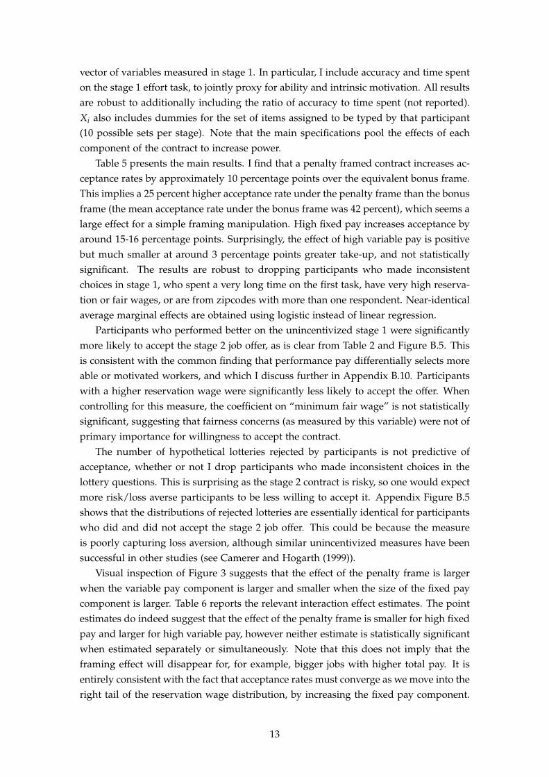
Visual inspection of Figure 3 suggests that the effect of the penalty frame is largerwhen the variable pay component is larger and smaller when the size of the fixed paycomponent is larger. Table 6 reports the relevant interaction effect estimates. The pointestimates do indeed suggest that the effect of the penalty frame is smaller for high fixedpay and larger for high variable pay, however neither estimate is statistically significantwhen estimated separately or simultaneously. Note that this does not imply that theframing effect will disappear for, for example, bigger jobs with higher total pay. It isentirely consistent with the fact that acceptance rates must converge as we move into theright tail of the reservation wage distribution, by increasing the fixed pay component.

13

In addition, the point estimate on “high variable pay” is essentially zero for participantsunder the bonus frame, implying that the potential for a $3 bonus as opposed to a $1.50bonus did not make the job offer significantly more attractive.

3.2 Selection

Now I turn to the effect of the penalty frame on the types of workers that select intothe contract. Figure 4 plots CDFs of stage 1 task performance, time spent on stage 1task, rejected lotteries, reservation wage and fair wage, comparing those who acceptedthe bonus frame with those who accepted the penalty frame. Surprisingly, the dis-tributions are overlapping for all variables except for reservation wages, implying nonotably differential selection on these variables.27 I do observe suggestive evidence thatthe penalty contract attracted workers with higher reservation wages. This is not incon-sistent with no selection on other characteristics, since as shown in Appendix B.2, thecorrelation between reservation wages and other characteristics is small.

Table 7 tests for selection effects of penalty framing by interacting the penalty framewith the key observables in acceptance regressions. The interaction coefficients estimatethe extent to which a given characteristic more or less strongly predicts acceptance un-der the penalty frame. In each case the interaction terms are not statistically significant,whether estimated separately or jointly. A joint test fails to reject the null that all inter-action coefficients are equal to zero (p-value 0.90).

In Appendix B.5 I check if the results are robust to dropping outliers for time spenton task 1, reservation wage and fair wage, or dropping participants who made incon-sistent lottery choices. The only difference is that now the interaction between penaltyframe and reservation wage is significant at the 10 percent level, consistent with thepenalty screening in participants with higher reservation wages. Overall there is littleevidence of selection on these key observables between contract types.

As for the other covariates, men and women are equally likely to accept the penaltycontract, but men are eleven percentage points less likely to accept the bonus contract.In other words, men are less likely than women to accept the incentivized task in gen-eral, but relatively more likely to prefer the penalty to the bonus contract. Participantswho reported that their main reason for working on MTurk is to earn money (93 percentof participants) are relatively more likely to accept the penalty contract than those whogave another reason, similar applies to those who report mostly working on researchHITs. Participants with more HITs completed are relatively less likely to accept thebonus contract. Despite the fact that being male and citing money as the main reasonfor working are positively associated with performance on stage 1, none of these resultsseems to be consequential for performance, as illustrated by the lack of selection onstage 1 performance measures and the evidence presented in the next section.

It is quite surprising that there seems to be no selection effect of penalty framing.

27The equivalent “balance” figures in Appendix B.3 confirm that this finding represents balance beforeand after candidates accepted the offer, not an initially unbalanced situation that became balanced bychance after acceptance decisions.

14

One possibility is that selection is hard to detect in this context. If workers could choosebetween the bonus and penalty framed job (assuming this did not undo the framingeffect) they should select into the job they preferred. However in this experiment,workers cannot choose jobs, only whether to accept the one that they are offered. Asa result there will be many participants in each pool whose participation constraintswould be satisfied under either contract: any selection effect would have to be drivenby the fraction of participants whose participation constraints are satisfied under onebut violated under the other. However, given the large difference in acceptance ratesbetween contracts it seems unlikely that this is what is driving the lack of detectableselection. In addition, as documented in Appendix B.10, I am able to observe the morestandard result of differential selection by type into the incentivized task: workers withhigh performance in the first stage are more likely to accept the job in the second stage.

3.3 Performance

Now I turn to the incentive effects of contract framing on worker effort and perfor-mance. This section directly relates to the existing literature on framed contracts whichconsiders incentive effects for an already recruited sample of workers or participants.

The basic regression equation is:

Yi = δ0 + δ1 ∗ Penaltyi + δ2 ∗ HighFixedi + δ3 ∗ HighVariablei + δ4 ∗ Xi + εi (6)

Where Yi is a measure of effort or performance. The key measures are summarized inTable 2 and distributions plotted in Appendix Figure B.1. As before, Xi is a vector ofvariables measured in stage 1.

In general one would expect the estimates of δ1, δ2 and δ3 to be biased by selec-tion: if the workers that accept one type of contract are different from those that acceptanother, then performance differences may simply reflect different types rather than dif-ferent effort responses to incentives. However as already documented, I do not observenotably differential selection between frames, which would bias the estimate of the keycoefficient of interest, δ1. Moreover, since I have stage 1 measures of performance andcharacteristics, I can control for selection on observables by including these.

Figure 5 presents the mean performance on the stage 2 task by treatment group. Ifind that performance is higher under the penalty than under the bonus frame, consis-tent with the existing experimental studies. Pooling each framing treatment, in Figure6 I plot CDFs of the accuracy measure, the log distance measure (recall that this isinterpreted as the log of the per-character error rate) and time spent, and find thatperformance and effort is higher under the penalty frame right across the distribution.

The main regression results are given in Table 8. I find that accuracy under thepenalty frame is around 3.6 percentage points (around 0.18 standard deviations or 6percent of the mean accuracy of 0.59) higher than under the bonus frame, statisticallysignificant at 5 percent without and 1 percent with controls. The coefficient estimateis robust to dropping participants who made inconsistent lottery choices, participants

15

from zipcodes with multiple respondents, and outliers on the reservation and fair wagequestions (although a little smaller and only significant at 10 percent). Crucially, the es-timated penalty effect is unaffected by the inclusion or exclusion of controls, consistentwith the contract frame not inducing significant outcome-relevant selection, at least onobservables. For selection to explain the results, there would have to be a substantialunobserved driver of performance that differentially selected under the penalty frameand orthogonal to the set of controls included in the regressions.28

In addition, high fixed pay increases accuracy by around 2-4 percentage points,significant at 5 percent when controls are included. The point estimate doubles whencontrols are included, suggesting there may be adverse selection induced by the higherfixed pay. If anything, the fact that a selection effect is observed here gives comfort thatthe lack of observed selection between bonus and penalty reflects a true lack of selectionin the data. Lastly, high variable pay increases accuracy by around 1.4-2.5 percentagepoints, although this is never significant at conventional levels.

As for the other key variables, performance in the first stage very strongly predictsperformance in the second stage, while the coefficient on time spent in the previoustask is negative, small in magnitude and not significant. As in stage 1 (see AppendixB.2), a higher reservation wage is associated with poorer performance. Controlling forthe reservation wage, the reported minimum fair wage has no effect on performance,consistent with fairness concerns not being of primary import.

In this stage the number of rejected lotteries is negatively associated with perfor-mance, significant at ten percent when including participants who made inconsistentchoices and five percent when they are dropped. A one standard deviation increase inthe number of rejected lotteries is associated with around 1-2 percentage points worseperformance. This result relates to Prediction 2 and is expanded upon when I considerheterogeneous effects below.

In Table 9 I separate the effects of increasing fixed and variable pay under bonusand penalty framing. Increasing the fixed pay seems to have the same effect underboth bonus and penalty contracts (the interaction effect is an imprecisely estimatedzero). Increasing the size of the variable pay is associated with higher effort under bothframes, with a smaller effect under the penalty frame. However neither estimate isstatistically significant.

Table 10 reports estimates of heterogeneous effects of the penalty treatment by themain variables. In each case the individually estimated interaction effect is not statisti-cally significant: there is little evidence of strong heterogeneous effects.29

28In Appendix table B.4 I regress the distance measure of accuracy (log errors per character typed)and time spent on treatment dummies and covariates. The estimates imply that the penalty frame ledto participants committing 20 percent fewer errors per character (from a mean of 0.066), and spendingaround two to three minutes longer on the task (mean 41 minutes), although the latter is not significantwhen controls are included. The point estimates on fixed and variable pay mirror their counterparts in themain regressions, and once again there is evidence of adverse selection induced by the higher fixed pay.

29Including all of the interaction effects estimated together gives one unexpected and difficult to interpretresult: a negative interaction effect for reservation wages and a positive one for minimum fair wages.Dropping participants above the 99th percentile for reservation or fair wages, the p-value on the reservationwage interaction increases to 0.09 and that on the fair wage interaction increases to 0.14.

16

Focusing on the coefficient on rejected lotteries, I note that although neither the maineffect nor interaction coefficient are statistically significant, nevertheless it is strikingthat the implied coefficient on rejected lotteries is close to zero under the bonus frame,and negative under the penalty frame (the combined effect under the penalty frameis statistically significant at the 5 percent level), while the model Prediction 2 impliesthat the coefficient should be more positive under the penalty frame. Note also that themodel predicts a positive relationship between loss aversion and performance, whereasI find a negative one. An extension that allows the reference point to also depend uponexpectations, outlined in Appendix A.3, can allow for this finding.

I lack power to dig into this relationship in depth. I do however perform one sim-ple exercise. In Figure 8 I non-parametrically plot accuracy against rejected lotteriesseparately under bonus and penalty frame, after partialling out the other variables,dropping participants with inconsistent choices and those who rejected or accepted alllotteries. The slopes are approximately equal over much of the range of values forrejected lotteries, but flattening out for high values under the bonus frame while be-coming strongly negative under the penalty frame, which seems to be what is what isdriving the difference in the regression coefficients. For most participants the relation-ship between performance and loss aversion is similar between frames, but penaltiesseem to strongly discourage the most loss averse participants, an effect which is not inthe model.

The surprising implication of the results is that a simple switch from bonus topenalty framing is very lucrative from the principal’s perspective. My estimates suggestthat recruitment and performance would be approximately equal under a contract thatpays $0.50 fixed pay with $1.50 variable pay framed as a penalty, as with $1.50 fixedpay and $1.50 variable pay, framed as a bonus.

4 Secondary Results

In this section I discuss secondary results aimed at partly unpacking the mechanismbehind the main results. First, I demonstrate that the penalty frame did not appearto change participants’ perceptions of the task difficulty (I find the same result in thefollow-up survey described in section 5.1). Second, I argue that inattention is unlikelyto explain the higher acceptance rate of the penalty contract.

Additionally, in Appendix B.9, I discuss persistence, showing that the performancedifference between bonus and penalty frame persisted throughout stage 2. If workersquickly realized the equivalence of the frames, one would expect performance to con-verge. In Appendix B.10 I document that a standard selection result is present in mydata: performance pay attracted more able workers, which partly explains the differ-ence in stage 1 and stage 2 performance. This gives confidence that the no-selectionresult between frames is not driven by, for example, MTurk workers being atypicalexperimental subjects.

17

4.1 Does framing affect perceived task difficulty?

At the beginning of the stage 2 task, subjects were asked to predict the overall meanaccuracy rating from the first stage. If the frame influenced their beliefs about thetask difficulty, it should also influence their belief about mean performance in the firststage. Figure 7 graphs the mean of these predictions by treatment group. There is nosystematic relationship between the framing treatment and the predictions.

In Appendix B.7 I regress the participants’ estimates on the treatment and the samecontrols as the main regressions. As expected, I find no evidence that the frame influ-enced participants’ beliefs about the task difficulty: I can rule out a difference largerthan ±3 percent at the 95 percent level. In sum, it does not appear that the effect of thepenalty contract is explained by different beliefs induced by the frame.30

4.2 Inattention: Comparing Sessions 1 and 2

After running the first experimental session, one concern was that the way in whichthe job offer was phrased might differentially attract inattentive participants into thepenalty frame, explaining the higher acceptance rate. The “pay” section of the offeremail under the bonus (penalty) frame was written as follows:

The basic pay for the task is $0.50 ($3.50). We will then randomly select oneof the 50 items for checking. If you entered it correctly (incorrectly), the paywill be increased (reduced) by $3.00.

It is possible that an inattentive participant receiving the bonus email might glance atthe first sentence, see a low amount and close the message, while under the penaltyframe she might see the high amount and click through to the task.31 To alleviate thisconcern, the second session changed the email slightly, as follows:

The pay for this task depends on your typing accuracy. We will randomlyselect one item for checking, and if it was entered correctly (incorrectly), thepay will be increased above (reduced below) the base pay. The base pay is$0.50 ($3.50) which will be increased (reduced) by $3 if the checked item iscorrect (incorrect).

This phrasing pushes the pay information to the end of the paragraph and puts it allinto one sentence. It also tells the participants immediately that the pay will depend onperformance, and hence they should pay attention to the contingent component of pay.

30I do find that participants assigned the high bonus predict that stage 1 accuracy was 3.5 percentagepoints higher. To check whether this affected stage 2 performance, I also regress stage 2 performance onthe main regressors, now including the participant’s prediction of stage 1 accuracy. In the specificationwith only treatment indicators I find a strong and significant correlation between predicted and actualperformance, perhaps because the predictions are positively (although not significantly) correlated withown performance on task 1, which is in turn a strong predictor of task 2 performance. Taken literally, thecoefficient implies that a 10 percentage point higher belief about mean stage 1 performance is associatedwith 2 percentage points better performance in stage 2. When controls are included, this coefficient dropseffectively to zero and is not statistically significant.

31Note, however, that this is only part of the email content and that “base pay” should strongly signifythat there is more payoff-relevant information to come.

18

Of course, one challenge with interpreting such manipulations is that if no effect wereobserved, it is hard to tell whether the rephrasing eliminated inattention, or somehowchanged the reference point.

As shown in Figure 3, the penalty framed offer was again strongly more attractivethan the bonus framed offer in session 2, with an acceptance rate of 48 percent under thepenalty and 37 percent under the bonus, suggesting that inattention does not explainthe main results. I do find that the performance difference between bonus and penaltywas much smaller and not significant in session 2 (see Figure 5). I confirm in this bysplitting the penalty treatment effect by session in regressions in Appendix B.8. It is notpossible to say whether this is a treatment effect (the rephrasing decreased the framingeffect on performance) or sampling variation.

5 Why are penalties popular?

The acceptance rate is substantially higher under the penalty frame than under thebonus frame, contradicting model Prediction 3. While loss aversion can explain thehigher effort provision under the penalty contract, it cannot explain the higher accep-tance rate, suggesting that participants may be maximizing a different objective functionwhen deciding whether to accept the job than when performing the task.32

Participants appear to be failing to anticipate the loss they will experience if un-successful, should they take accept the job.33 It could be that the temporal separationbetween doing the task and realization of the payment a few days later is sufficient thatparticipants do not anticipate being strongly disappointed when unsuccessful underthe penalty frame. However, clearly this is not enough to explain the higher acceptancerate under the penalty contract, since complete failure to anticipate loss aversion shouldimply indifference between the two contracts.

An obvious candidate explanation is that participants anticipate they will workharder and earn more under the penalty contract, which makes it attractive. This argu-ment requires three parts. First, that the loss when unsuccessful is not anticipated asbeing sufficiently painful to discourage acceptance, for instance because the “planner”self who accepts the offer is not averse to losses experienced by the “doer” self whodoes the work. Second participants must recognize that they will work harder underthe penalty frame. Third, effort provision under the bonus frame must be suboptimallylow, such that being motivated to work harder is attractive. In other words, it requiresa self-control problem, where penalties act as a commitment device.34

As a simple example, suppose that when deciding whether to accept the contract,

32As such, the following discussion relates to multiple-selves models e.g. Thaler and Shefrin (1981),Fudenberg and Levine (2006).

33This point relates to the literature on anticipating preferences or biases. For example, Loewensteinand Adler (1995) find that people underestimate the endowment effect: they predict a lower willingnessto accept to give up a mug when asked to imagine being endowed with it than when actually endowedwith it. See also Loewenstein et al. (2003) for related discussions.

34This point is closely related to the goal-setting literature, particularly Koch et al. (2012) and Golmanand Loewenstein (2012).

19

A evaluates it according to the following modified utility function:

V(w, b, e∗(w, b, F)) = w + 2e∗(w, b, F)b− βe∗2(w, b, F)

2γ+ αe∗(w, b, F). (7)

(7) is chosen to coincide with (1) when λ = β = 1 and F = 0, in other words, whenA does not expect (or is not averse to) losses. V depends on e∗(w, b, F), reflecting thatA knows that if she accepts the contract she will choose her effort according to (3). Aprefers the penalty frame (F = 1) if V(w, b, e∗(w, b, 1)) > V(w, b, e∗(w, b, 0)).

From the perspective of an agent maximizing V, the first-best effort choice is eFB =γ[α+2b]

β = e∗(w,b,0)β . It is clear therefore that a necessary condition for A to prefer penalty

frames is eFB > e∗(w, b, 0), or β < 1. One interpretation of this condition is that Ahas weak self-control and is sophisticated about it: she knows she will exert less effortthan she would like to. A simple sufficient condition for this self-control problem to besufficiently severe that the penalty is preferred is eFB ≥ e∗(w, b, 1) or α+2b

α+b(1+λ)≥ β.

It is certainly plausible that workers might like penalty contracts as a commitmentdevice, an idea reminiscent of recent evidence from Kaur et al. (2013), who find thatworkers select into a strictly dominated financial incentive scheme that acts as a formof commitment to higher effort provision. However, in my context it seems unlikelythat this is what is driving the large differences in acceptance rates between bonus andpenalty frames, because the associated earnings difference is small (not even accountingfor the higher effort cost under penalties). In Table 11 I compute what would be theaverage rational expectation of earnings for each treatment, computed as fixed payplus the product of mean task 2 accuracy and variable pay. The increase in expectedearnings when switching from bonus to penalty framing is never more than 10 cents,but generates around 10 percentage points higher acceptance. Meanwhile increasingthe fixed pay by $1.50 (which increases expected pay by just over $1.50 after accountingfor effort) increases acceptance by 19 percentage points. As previously noted, increasingthe variable pay under the bonus frame has no appreciable effect on acceptance, despiteincreasing expected earnings by around 90 cents.

These results suggest that workers do not have rational expectations about theirearnings, or are somehow failing to correctly weight the terms of the contract. Themost likely explanation is that participants are focusing on the “base pay”, which ishigher under the penalty contract, and underweight the bonus or penalty component.Thus the base pay both shifts their reference point (driving differences in effort) andtheir valuation of the contract. A simple reduced form way to model this is to simplyassume that the frame, F, enters additively on the left hand side of A’s participationconstraint.

Participants may be evaluating the terms of the contract separately, instead of in-tegrating them into an expectation. In other words, they are acting as if they havepreferences over base pay and contingent pay, rather than over outcomes. The con-tract (w, b, F) is perceived as (base pay, bonus, penalty) = (w + Fb, (1− F)b, Fb) suchthat (w + b, 0,−b) � (w, b, 0), rather than as a lottery that pays w + b with probability

20

e and w with probability 1 − e. Essentially, base pay is overweighted when evaluat-ing whether to accept: ($3.50, $0,−$3) feels more lucrative than ($0.50, $3, $0). Thispossibility is closely related to the finding of Hossain and Morgan (2006), that in on-line auctions for identical goods, the total sale price (winning bid plus shipping cost)is higher when the shipping cost is higher (revenue equivalent predicts that the totalprice should not depend the proportion labeled as shipping costs). Hossain and Mor-gan (2006) suggest a mental accounting explanation, whereby goods and shipping areassigned separate mental accounts and are subadditively weighted.

The findings might also reflect a form of “Coherent Arbitrariness” (Ariely et al.(2003)). An agent with coherently arbitrary preferences is vulnerable to arbitrary ma-nipulations of her valuation of a good or experience (for example, her valuation of agood can be altered by priming her with a transparently uninformative random num-ber). In this context, participants’ valuations of the contract are influenced by the num-ber presented as base pay, which is higher under the penalty contract.

A third mechanism that would manifest as an apparent preference for high basepay is analyzed theoretically by Just and Wu (2005) and Hilken et al. (2013). In theirmodels, the contract and outside option are both evaluated against the same referencepoint, which is influenced by the frame. By increasing the reference point, the penaltyframe makes the contract appear more attractive relative to the outside option.

5.1 Evidence

To shed some additional light on mechanisms, I conducted a short survey four daysafter experimental session 2 ended, asking participants their perceptions of the joboffers. The questions are unincentivized and mostly subjective, and the survey wasconducted after completion and payment of stage 2 which might affect responses, sothe results should be taken with a large pinch of salt. All participants from stage 1 ofsession 2 were invited to complete a survey for a fixed incentive of $2. 82 percent did,balanced between the bonus and penalty frame.35

Participants were first reminded of the job offer they received, then asked a seriesof questions about it. Appendix table B.8 presents results. Participants were asked toindicate agreement on a 1-7 scale to whether their job offer or task was fun, easy, paidwell, fair, was a good motivator, whether the principal could be trusted, achievable36

and understandable (Panel A). They were then asked to what extent they agreed thatvarious features made the offer attractive or unattractive (Panel B). Third, they wereasked to guess mean acceptance and performance of participants who received thesame job offer as they did.

For most questions I find no significant differences between frames. However thepenalty offer was rated significantly higher (about 0.3 s.d., significant at 5 percent)

35Participants who completed stage 2 were more likely to complete the survey (96 percent vs 73 percent,p-value < 0.001), probably reflecting that some non-participation in stage 2 is driven by participants whodid not see my emails.

36“If a participant worked hard on the task, he or she can be confident that they would answer thechecked item correctly.”

21

for “good pay” and was more likely to be considered attractive due to good pay. Ifanything, the penalty was perceived as a less good motivator and less attractive for itsmotivational power than the bonus contract.

The second finding is that estimated acceptance rates and performance were notsignificantly different between bonus and penalty frames. It is possible that althoughthe penalty increases a participant’s own valuation and effort, they fail to recognize itwill have this effect on others. Of course an alternative explanation is that participantswere simply unable to make an informed guess.37

Overall I interpret the survey results as suggestively supporting the idea that thepenalty contract, via its high “base pay”, was viewed as more lucrative. They do notappear to support penalties being valued as a commitment device, although note thatthis reasoning is more complex to articulate and so perhaps harder to detect via surveyquestions.

5.2 Discussion

Although a demand for commitment story or overweighting of the base pay may ex-plain why penalties were more popular, four findings remain outside the model andwould benefit from further theoretical and empirical work.

First, participants exert higher effort when the fixed pay component is increased.The most obvious explanation here is reciprocity in response to perceived generosityfrom the principal (increasing the fixed pay).38

Second, it is surprising that a $1 increase in the variable pay seems to have at mosta small and not statistically significant effect on acceptance and performance, while a$1 increase in the base pay (with no change in material incentives) has a large effect.

Third, given the size of the effect of the penalty frame on acceptance rates, it isvery striking that there is apparently no selection effect of incentive framing on theobservables measured. Almost any model is likely to predict adverse or advantageousselection. It would be particularly interesting to see whether this finding replicates inother settings.

Fourth, the relationship between incentivized performance and loss aversion, mea-sured by rejected lotteries, remains something of a puzzle. First, I find a negativerelationship, which is inconsistent with the model outlined in section 1 but is possible

37At the end of the survey, I also presented participants with the alternative contract frame that theycould have received and asked them to compare it to the one they did receive on generosity, motivationalpower, et cetera. Unsurprisingly, I find no significant differences between frames, consistent with subjectsrealizing the equivalence of the two. I also asked subjects how likely they would be, on a 5 point scale,to accept the job if it were offered to them again, to get a sense of how penalty contracts might performin a repeated contracting environment. I find no significant difference in willingness to re-accept betweenbonus and penalty contract. Conditional on stage 2 performance, workers who were lucky (the item Ichecked was one of the ones they answered correctly) reported 0.6s.d. higher “likelihood”.

38Alternatively, perhaps some participants believed that maintaining a good reputation with the princi-pal would be rewarded in future, and higher fixed pay increased the perceived value of a good reputation.Participants were explicitly told in the first stage that the chance of being invited for future tasks wouldnot depend on their performance, but this was not reiterated in the second stage. To explain the highereffort in all treatments under the penalty contract this reputation mechanism would have to be strongerfor penalties than bonuses.

22

under a generalization that also allows the reference point to depend upon expectations,given in Appendix A.3. However, both predict a relatively more positive relationshipunder the penalty frame, which I do not observe. I presented evidence (albeit suggestiveat best) that penalties may have a discouragement effect on the most loss-averse par-ticipants. This again would benefit from further research to unpack how loss aversiondrives the effect of penalties.

6 Conclusion

This paper analyzes the effects of framed incentive pay on worker recruitment, selec-tion and performance. I find that penalty framed incentives increased the number ofworkers who accepted the job by 25 percent relative to economically equivalent bonusframed incentives. In addition the penalty frame increased performance on the job by6 percent, around 0.2 standard deviations. The effect sizes are large relative to thosefor standard manipulations of incentive size: increasing the non-contingent pay from$0.50 to $2 increased the acceptance rate by 36 percent and performance by 0.2 standarddeviations, while the effect on both outcomes of increasing the contingent componentof pay from $1.50 to $3 was small and statistically insignificant. Interestingly, I find noevidence of either adverse or advantageous selection into the penalty framed contract,while I do find advantageous selection into the incentivized task as a whole.

I present further evidence that the relative attractiveness of the penalty frame isnot driven by changed perceptions of the difficulty of the task, nor is it driven by thewording of the job offer that might differentially attract inattentive workers. I also showin the appendix that a standard selection result obtains in this context, namely that thejob offer with incentive pay attracted relatively high ability participants, and that theeffect of the framed incentive on performance did not wear off during the course of theexperiment.

While loss aversion, combined with an assumption that penalty framing increasesthe agent’s reference point, predicts higher effort under the penalty frame, it also pre-dicts that agents should be less willing to accept a penalty framed contract than theequivalent bonus contract, because agents anticipate that they will be more disap-pointed under the penalty contract. I propose two possible extensions that might ex-plain why I find the opposite. One possibility is that agents like penalties because theymotivate them to work harder, overcoming a self control problem, in a similar spirit torecent findings by Kaur et al. (2013). Alternatively, workers may be evaluating contractoffers as if they had preferences over their constituent components (base pay, bonus,penalty), rather than over outcomes, and may be attracted by the salient high base payunder the penalty contract, similar to how eBay bidders apparently fail to correctlycombine the cost of shipping and the price of the good when bidding (Hossain andMorgan (2006)). The fact that earnings were in practice very similar between bonus andpenalty participants seems to go against them being particularly valuable for overcom-ing weak self-control. Meanwhile, a follow-up survey found that participants perceived

23

the penalty offer as more generous, suggestively supporting the second mechanism.Overall, the results are surprising, suggesting that from the principal’s perspective,

penalty contracts may strongly outperform bonus contracts in some settings. In envi-ronments similar to the experimental context, such as short-term one-off engagements,firms may be able to gain through greater use of penalties. However to answer themotivating question of why firms seem reluctant to use penalties in general, it is clearthat more research is needed.

The results and proposed mechanisms suggest that the answer may lie in dynamics.In practice, many contracting arrangements are repeated or long-term, and the contractmust satisfy not only a participation constraint at the time of acceptance, but on an on-going basis, to prevent workers from quitting. Meanwhile, it seems reasonable to expectthat framing effects will eventually wear off: the agent’s reference point adjusts, mod-erating the commitment power of the contract, or her rosy perception of the job offeradjusts over time to reflect what she sees on her payslips. Thus the higher acceptancerate under penalty contracts may also lead to a higher quit rate, which is costly for theemployer.39 Moreover, as the worker’s reference point adjusts, the effect of the frame onher effort wear off as well, eliminating the contract’s performance advantages.40 Sucheffects may partly explain why firms are reluctant to use penalty frames.

References

Abeler, J., A. Falk, L. Goette, and D. Huffman (2011). Reference Points and EffortProvision. American Economic Review 101(2), 470–492.

Amir, O., D. G. Rand, and Y. K. Gal (2012, January). Economic games on the internet:the effect of $1 stakes. PloS one 7(2), e31461.

Ariely, D., G. Loewenstein, and D. Prelec (2003, February). "Coherent Arbitrariness":Stable Demand Curves Without Stable Preferences. The Quarterly Journal of Eco-nomics 118(1), 73–106.

Armantier, O. and A. Boly (2012). Framing of Incentives and Effort Provision. mimeo.

Baker, G., M. Jensen, and K. Murphy (1988). Compensation and Incentives: Practice vs.Theory. The Journal of Finance 43(3), 593–616.

Barankay, I. (2011). Rankings and Social Tournaments: Evidence from a Crowd-Sourcing Experiment. mimeo, 1–30.

Bénabou, R. and J. Tirole (2003, July). Intrinsic and Extrinsic Motivation. The Review ofEconomic Studies 70(3), 489–520.

Bordalo, P., N. Gennaioli, and A. Shleifer (2012, April). Salience Theory of Choice UnderRisk. The Quarterly Journal of Economics 127(3), 1243–1285.

Brooks, R. R. W., A. Stremitzer, and S. Tontrup (2013). Stretch It but Don’t Break It: TheHidden Risk of Contract Framing. Working paper.

39Salant and Siegel (2013) discuss this mechanism in the context of sales and returns of goods.40I do not see such effects over the brief duration of my study (see Appendix B.9), but Jayaraman et al.

(2014) do see only short-lived “behavioral” responses to a contract change.

24

Camerer, C., L. Babcock, G. Loewenstein, and R. Thaler (1997, May). Labor Supplyof New York City Cabdrivers: One Day at a Time. The Quarterly Journal of Eco-nomics 112(2), 407–441.

Camerer, C. and R. Hogarth (1999). The effects of financial incentives in experiments: Areview and capital-labor-production framework. Journal of Risk and Uncertainty 19(1-3), 7–42.

Church, B. K., T. Libby, and P. Zhang (2008, December). Contracting Frame and Individ-ual Behavior: Experimental Evidence. Journal of Management Accounting Research 20(1),153–168.

Crawford, V. P. and J. Meng (2011, August). New York City Cab Drivers’ Labor SupplyRevisited: Reference-Dependent Preferences with Rational-Expectations Targets forHours and Income. American Economic Review 101(5), 1912–1932.

de Meza, D. and D. Webb (2007). Incentive design under loss aversion. Journal of theEuropean Economic Association 5(March), 66–92.

Dohmen, T. and A. Falk (2011, April). Performance Pay and Multidimensional Sorting:Productivity, Preferences, and Gender. American Economic Review 101(2), 556–590.

Druckman, J. N. (2001, April). Using Credible Advice to Overcome Framing Effects.Journal of Law, Economics, and Organization 17(1), 62–82.

Eriksson, T. and M. C. Villeval (2008). Performance-pay, sorting and social motivation.Journal of Economic Behavior & Organization 68(2), 412 – 421.

Farber, H. S. (2005, February). Is Tomorrow Another Day? The Labor Supply of NewYork City Cabdrivers. Journal of Political Economy 113(1), 46–82.

Farber, H. S. (2008, May). Reference-Dependent Preferences and Labor Supply: TheCase of New York City Taxi Drivers. American Economic Review 98(3), 1069–1082.

Fehr, E. and S. Gächter (2002). Do Incentive Contracts Undermine Voluntary Coopera-tion? IEW Working Paper No. 34.

Fryer, R. G., S. D. Levitt, J. List, and S. Sadoff (2012). Enhancing the Efficacy of TeacherIncentives Through Loss Aversion: A Field Experiment. NBER working paper 18237.

Fudenberg, D. and D. K. Levine (2006). A Dual-Self Model of Impulse Control. AmericanEconomic Review 96(5), 1449–1476.

Gill, D. and V. Prowse (2012, February). A Structural Analysis of Disappointment Aver-sion in a Real Effort Competition. American Economic Review 102(1), 469–503.

Golman, R. and G. Loewenstein (2012). Expectations and Aspirations: Explaining Am-bitious Goal-setting and Nonconvex Preferences. mimeo.

Guiteras, R. P. and B. K. Jack (2014). Incentives, Selection and Productivity in LaborMarkets: Evidence from Rural Malawi. NBER Working Paper 19825.

Hannan, R. L., V. B. Hoffman, and D. V. Moser (2005). Bonus Versus Penalty: Does Con-tract Frame Affect Employee Effort? In A. Rapoport and R. Zwick (Eds.), ExperimentalBusiness Research, Vol II, Volume II, Chapter 8, pp. 151–169. Netherlands: Springer.

Herweg, F., D. Müller, and P. Weinschenk (2010, December). Binary Payment Schemes:Moral Hazard and Loss Aversion. American Economic Review 100(5), 2451–2477.

Hilken, K., K. D. Jaegher, and M. Jegers (2013). Strategic Framing in Contracts. TjallingC. Koopmans Research Institute Discussion Paper Series 13-04.

25

Horton, J. J., D. G. Rand, and R. J. Zeckhauser (2011, February). The online laboratory:conducting experiments in a real labor market. Experimental Economics 14(3), 399–425.

Hossain, T. and J. A. List (2012, July). The Behavioralist Visits the Factory: IncreasingProductivity Using Simple Framing Manipulations. Management Science 1909, 1–17.

Hossain, T. and J. Morgan (2006). ...Plus Shipping and Handling: Revenue (Non) Equiv-alence in Field Experiments on eBay. Advances in Economic Analysis & Policy 6(2),Article 3.

Jayaraman, R., D. Ray, and F. de Vericourt (2014). Productivity Response to a ContractChange. NBER working paper 19849.

Just, D. and S. Wu (2005). Loss aversion and reference points in contracts. mimeo.

Kahneman, D. and A. Tversky (1979, January). Prospect Theory: An Analysis of Deci-sion under Risk. Econometrica 47(2), 263–292.

Karlan, D. S. and J. Zinman (2009). Observing Unobservables: Identifying InformationAsymmetries With a Consumer Credit Field Experiment. Econometrica 77(6), 1993–2008.

Kaur, S., M. Kremer, and S. Mullainathan (2013). Self-Control at Work. mimeo.

Koszegi, B. (2014). Behavioral Contract Theory. Journal of Economic Literature Forthcom-ing.

Koszegi, B. and M. Rabin (2006, November). A Model of Reference-Dependent Prefer-ences. The Quarterly Journal of Economics 121(4), 1133–1165.

Koszegi, B. and M. Rabin (2007, September). Reference-Dependent Risk Attitudes.American Economic Review 97(4), 1047–1073.

Koch, A. K., J. Nafziger, A. Suvorov, and J. van de Ven (2012). Self-Rewards and PersonalMotivation. Working paper.

Lazear, E. (2000, February). Performance pay and productivity. The American EconomicReview 90(5), 1346–1361.

Lazear, E. P. (1995). Personnel Economics. MIT Press.

Loewenstein, G. and D. Adler (1995, July). A Bias in the Prediction of Tastes. TheEconomic Journal 105(431), 929.

Loewenstein, G., T. O’Donoghue, and M. Rabin (2003, November). Projection Bias inPredicting Future Utility. The Quarterly Journal of Economics 118(4), 1209–1248.

Luft, J. (1994, September). Bonus and penalty incentives contract choice by employees.Journal of Accounting and Economics 18(2), 181–206.

Pope, D. and M. Schweitzer (2011). Is Tiger Woods loss averse? Persistent bias inthe face of experience, competition, and high stakes. The American Economic Re-view 101(February), 129–157.

Rabin, M. (2000). Risk Aversion and Expected-Utility Theory: A Calibration Theorem.Econometrica 68(5), 1281–1292.

Salant, Y. and R. Siegel (2013). Contracts with Framing. Working paper.

Thaler, R. H. and H. Shefrin (1981). An Economic Theory of Self-Control. Journal ofPolitical Economy 89(2), 392–406.

26

Figures

Figure 2: Example screen from the typing task.

Session 1 Session 2

0

.1

.2

.3

.4

.5

.6

.7

($0.50, $1.50) ($0.50, $3.00) ($2.00, $1.50) ($0.50, $3.00)

BonusPenalty

Notes: financial incentive levels given in parentheses as (fixed pay, variable pay). Error bars indicate 95%confidence intervals.

Figure 3: Acceptance Rates by treatment.

27

0

.2

.4

.6

.8

1

Cum

ulat

ive

dens

ity

0 .2 .4 .6 .8 1Accuracy Rate Task 1

0

.2

.4

.6

.8

1

Cum

ulat

ive

dens

ity

0 .5 1 1.5 2Time Spent Task 1, hours

0

.2

.4

.6

.8

1

Cum

ulat

ive

dens

ity

0 3 6 9 12Rejected Lotteries

0

.2

.4

.6

.8

1

Cum

ulat

ive

dens

ity

0 3 6 9 12Reservation Wage, $/hr

0

.2

.4

.6

.8

1

Cum

ulat

ive

dens

ity

0 3 6 9 12Fair Wage, $/hr

Bonus Penalty

Figure 4: Comparing acceptors under Bonus and Penalty Frame. Reservation and fairwage trimmed at the 99th percentile.

28

Session 1 Session 2

0

.1

.2

.3

.4

.5

.6

.7

($0.50, $1.50) ($0.50, $3.00) ($2.00, $1.50) ($0.50, $3.00)

BonusPenalty

Notes: financial incentive levels given in parentheses as (fixed pay, variable pay). Error bars indicate 95%confidence intervals.

Figure 5: Accuracy by treatment.

0

.2

.4

.6

.8

1

Cum

ulat

ive

dens

ity

0 .2 .4 .6 .8 1Accuracy Rate Task 2

0

.2

.4

.6

.8

1

Cum

ulat

ive

dens

ity

-8 -6 -4 -2 0Log distance measure Task 2

0

.2

.4

.6

.8

1

Cum

ulat

ive

dens

ity

0 .5 1 1.5 2 2.5Time Spent Task 2, hours

Bonus

Penalty

Figure 6: Performance and effort measures, comparing bonus vs penalty frame. Timespent is trimmed at the 99th percentile.

29

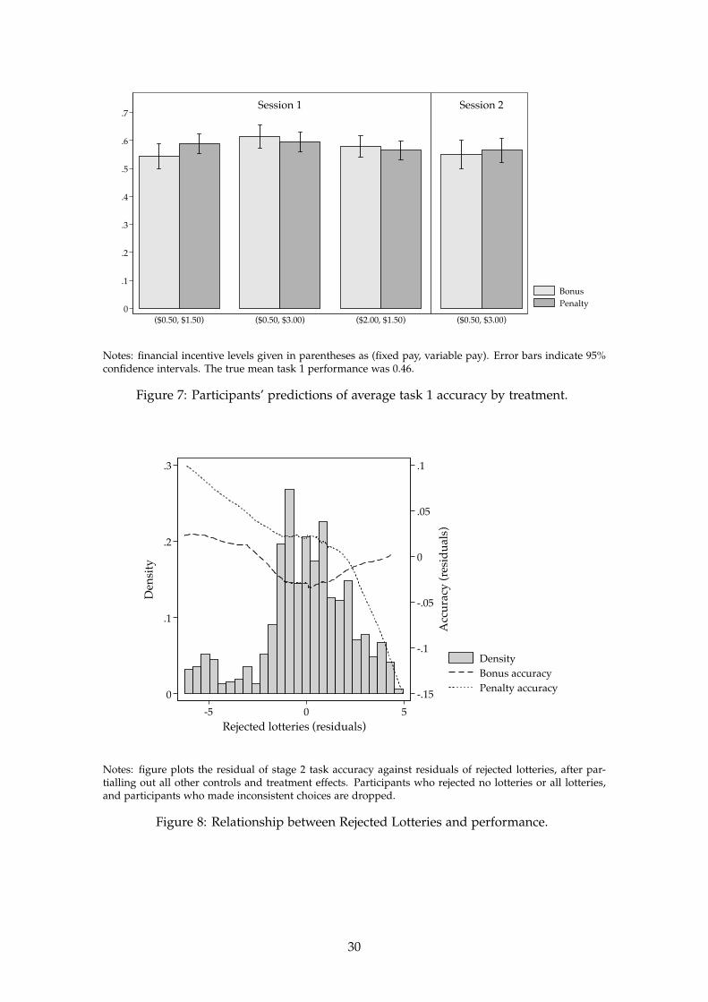
Session 1 Session 2

0

.1

.2

.3

.4

.5

.6

.7

($0.50, $1.50) ($0.50, $3.00) ($2.00, $1.50) ($0.50, $3.00)

BonusPenalty

Notes: financial incentive levels given in parentheses as (fixed pay, variable pay). Error bars indicate 95%confidence intervals. The true mean task 1 performance was 0.46.

Figure 7: Participants’ predictions of average task 1 accuracy by treatment.

-.15

-.1

-.05

0

.05

.1

Acc

urac

y (r

esid

uals

)

0

.1

.2

.3

Den

sity

-5 0 5Rejected lotteries (residuals)

DensityBonus accuracyPenalty accuracy

Notes: figure plots the residual of stage 2 task accuracy against residuals of rejected lotteries, after par-tialling out all other controls and treatment effects. Participants who rejected no lotteries or all lotteries,and participants who made inconsistent choices are dropped.

Figure 8: Relationship between Rejected Lotteries and performance.

30

Tables

Table 2: Performance on effort tasks

N Median Mean s.d.

Round 1Accuracy Task 1 1450 0.46 0.46 0.18Errors per item Task 1 1450 0.031 0.044 0.063Hours on Task 1 1448 0.60 0.67 0.31

Round 1, Rejectors onlyAccuracy Task 1 763 0.44 0.43 0.18Errors per item Task 1 763 0.033 0.048 0.070Hours on Task 1 761 0.62 0.69 0.32

Round 1, Acceptors onlyAccuracy Task 1 687 0.50 0.48 0.17Errors per item Task 1 687 0.028 0.039 0.053Hours on Task 1 687 0.57 0.64 0.28

Round 2Predicted Mean Round 1 Accuracy 686 0.60 0.58 0.19Accuracy Task 2 687 0.62 0.59 0.20Errors per item Task 2 687 0.017 0.066 0.17Hours on Task 2 686 0.62 0.75 1.24

“Accuracy” is the fraction of effort task items a participant entered correctly. “Errors per item” is com-puted as the mean of the Levenshtein distance between entered and correct answers, scaled by stringlength. “Hours on Task X” is estimated by multiplying the median page time by 10 to account for outliers.“Round 1, Acceptors (Rejectors) only” gives the stage 1 scores of the participants who accepted (rejected)the job offer in stage 2. “Predicted Mean stage 1 Accuracy” is the participant’s response to the question“Of the 50 items in the typing task you did before, how many do you think people entered correctly,on average?” Where timing data is missing (two observations in stage 1, one in stage 2) this is due toJavaScript errors. One participant did not report a predicted stage 1 accuracy.

31

Table 3: Summary Statistics from stage 1 Survey

N Mean s.d.

Loss AversionRejected Lotteries 1450 6.82 2.78Inconsistent Lottery Choices 1450 0.07 0.25

Reservation WageReservation wage, $/hr 1450 4.86 2.70Minimum fair wage, $/hr 1450 6.00 2.56

MTurk ExperienceHours working on MTurk per week 1450 16.5 15.3Typical MTurk earnings, $100/week 1450 0.58 0.58MTurk HITs completed 1450 7457 27548Months of experience on MTurk 1450 11.7 13.6Mainly participate in research HITs 1450 0.77 0.42Work on MTurk mainly to earn money 1450 0.93 0.26

DemographicsAge in 2013 1449 32.8 10.7Male 1450 0.49 0.50Household Income 1450 38362 27942Zipcode cluster 1450 0.13 0.34

Employment StatusFull time 1450 0.37 0.48Part time 1450 0.14 0.35Self employed 1450 0.10 0.30Full time MTurk worker 1450 0.11 0.31Unemployed 1450 0.12 0.33Student 1450 0.11 0.31Other 1450 0.05 0.21

EducationLess than High School 1450 0.00 0.07High School / GED 1450 0.11 0.31Some College 1450 0.32 0.472-year College Degree 1450 0.12 0.334-year College Degree 1450 0.35 0.48Masters Degree 1450 0.07 0.25Doctoral/Professional Degree 1450 0.02 0.13

“Rejected lotteries” is the number (0-12) of 50-50 win-lose lotteries that participants report they would beunwilling to play. “Inconsistent Lottery Choices” indicates participants who indicated inconsistent prefer-ences over lotteries (accepting a lottery dominated by one they rejected). “Minimum acceptable wage” isthe minimum hourly wage at which participants are willing to work on MTurk. “Minimum fair wage” isthe reported minimum fair hourly wage that requesters “should” pay on MTurk. “Mainly participate inresearch HITs” indicates participants who report mostly working on HITs posted by researchers. “Work onMTurk mainly to earn money” indicates participants main reason for working (“for fun”, “something else”coded as zero). “Male” is a dummy, note that six transgender individuals are coded as zeros. “Householdincome” is calculated using midpoints of income bins (“0-$30,000”, then $10,000 bins until “> $100,000”).Zipcode cluster is a dummy indicating at least one other participant in the same session reported the samezipcode. “Employment Status” and “Education” are sets of mutually exclusive dummy variables.

32

Table 4: Balance Check

Joint Groups 0 & 1 Groups 2 & 3 Groups 4 & 5 Groups 6 & 7

F-stat p Diff p Diff p Diff p Diff p

Accuracy Task 1 0.90 0.51 -0.01 0.54 0.00 0.94 -0.00 0.84 0.01 0.59Hours on Task 1 0.51 0.83 0.01 0.76 -0.00 1.00 0.01 0.68 -0.04 0.28Rejected Lotteries 0.53 0.81 0.31 0.26 -0.08 0.79 -0.23 0.39 -0.17 0.60Inconsistent Lottery Choices 0.62 0.74 0.01 0.60 0.02 0.42 -0.01 0.80 0.01 0.81Reservation wage, $/hr 0.65 0.72 0.07 0.77 -0.02 0.93 0.10 0.77 0.06 0.84Minimum fair wage, $/hr 2.87 0.01 0.08 0.73 0.05 0.88 -0.38 0.14 0.16 0.59Hours working on MTurk per week 1.65 0.12 -0.28 0.83 -1.61 0.21 -1.47 0.29 0.80 0.75Typical MTurk earnings, $100/week 0.35 0.93 -0.04 0.54 0.01 0.79 0.01 0.84 -0.00 1.00MTurk HITs completed 1.85 0.07 -7499.66 0.09 3609.55 0.07 460.60 0.71 -1966.82 0.50Months of experience on MTurk 0.67 0.70 1.04 0.49 0.50 0.68 -0.34 0.80 -1.55 0.37Mainly participate in research HITs 0.44 0.87 -0.04 0.39 0.04 0.38 -0.00 0.99 0.02 0.73Work on MTurk mainly to earn money 1.22 0.29 -0.03 0.31 -0.03 0.25 0.00 0.96 0.02 0.52Age in 2013 0.73 0.65 1.38 0.18 -0.80 0.45 -0.90 0.42 0.53 0.69Male 0.93 0.48 0.08 0.12 -0.00 0.93 0.01 0.92 -0.01 0.81

“Joint” reports the F-statistic and p-value from a joint test of the significance of the set of treatment dummies in explaining each relevantbaseline variable. The remaining columns report the difference in means and p-value from the associated t-test between pairs of treatmentgroups, where pairs differ only in terms of the bonus/penalty frame.

33

Table 5: Acceptance decision

OLS Logit (marginal effects)

(1) (2) (3) (4) (5) (6)Accepted Accepted Accepted Accepted Accepted Accepted

Penalty Frame 0.110*** 0.110*** 0.116*** 0.104*** 0.110*** 0.103***(0.026) (0.026) (0.029) (0.026) (0.025) (0.025)

High Fixed Pay 0.163*** 0.160*** 0.152*** 0.154*** 0.161*** 0.153***(0.036) (0.036) (0.041) (0.036) (0.035) (0.034)

High Variable Pay 0.027 0.025 0.008 0.020 0.016 0.022(0.037) (0.036) (0.040) (0.036) (0.032) (0.035)

Accuracy Task 1 0.312*** 0.136 0.337 0.282***(0.075) (0.352) (0.309) (0.074)

Accuracy Task 1 ^2 0.106 -0.055(0.380) (0.337)

Hours on Task 1 -0.139*** -0.197*** -0.164*** -0.170***(0.042) (0.059) (0.044) (0.047)

Rejected Lotteries 0.005 -0.007 0.004 0.005(0.013) (0.015) (0.013) (0.013)

Reservation wage -0.021*** -0.013 -0.016** -0.018**(0.005) (0.009) (0.005) (0.006)

Fair wage 0.004 -0.006 0.005 0.007(0.006) (0.009) (0.006) (0.006)

Session 2 -0.026 -0.011 -0.002 -0.012 -0.012(0.038) (0.038) (0.041) (0.038) (0.037)

Inconsistent Lottery Choices -0.065 -0.068(0.050) (0.051)

Set dummies Yes Yes Yes Yes Yes Yes

Controls No No Yes Yes No Yes

N 1450 1448 1146 1447 1450 1447R-squared 0.034 0.066 0.119 0.114Pseudo R-squared .024 .089Mean dep. variable 0.474 0.474 0.480 0.475 0.474 0.475

Dependent variable is a dummy indicating whether the participant accepted the job offer in stage 2.Columns (1)-(4) report OLS linear probability regressions, columns (5) and (6) present average marginaleffects logit equivalents to (1) and (4). Standard errors clustered at zipcode-session level in parentheses.+ p<0.10, * p<0.05, ** p<0.01, *** p<0.001. Two participants are missing timing variable and one missingage variable. Column (3) drops participants who made inconsistent lottery choices or who are above the99th percentile of reservation wage, fair wage or time spent on task 1, or who are from zipcodes withmore than one respondent in that session. “Set dummies” indicate the set of strings participants typed instage 1. “Controls” are Hours worked on MTurk per week, MTurk earnings per week, HITs completed,MTurk experience, “Mostly do research HITs”, “Mainly MTurk to earn money”, age, male, and income,occupation and education dummies. “Rejected lotteries” measured in standard deviations.

34

Table 6: Acceptance: Interactions

(1) (2) (3) (4)Accepted Accepted Accepted Accepted

Penalty Frame 0.104*** 0.128*** 0.072* 0.107*(0.026) (0.030) (0.036) (0.050)

High Fixed Pay 0.154*** 0.200*** 0.155*** 0.190***(0.036) (0.045) (0.036) (0.050)

Penalty * High Fixed Pay -0.092 -0.071(0.059) (0.071)

High Variable Pay 0.020 0.020 -0.014 0.004(0.036) (0.036) (0.045) (0.048)

Penalty * High Variable Pay 0.068 0.032(0.051) (0.062)

Set dummies Yes Yes Yes Yes

Controls Yes Yes Yes Yes

N 1447 1447 1447 1447R-squared 0.114 0.115 0.115 0.115Mean dep. variable 0.475 0.475 0.475 0.475

Dependent variable is a dummy indicating whether the participant accepted thejob offer in stage 2. Estimates from OLS linear probability model. Standard errorsclustered at zipcode-session level in parentheses. + p<0.10, * p<0.05, ** p<0.01,*** p<0.001. “Controls” are the full set of regressors from Table 5 specification(4). “Set dummies” indicate which set of strings participants typed in stage 1.

35

Table 7: Selection

(1) (2) (3) (4) (5) (6) (7)Accepted Accepted Accepted Accepted Accepted Accepted Accepted

Penalty Frame 0.104*** 0.104*** 0.104*** 0.104*** 0.104*** 0.104*** 0.104***(0.026) (0.026) (0.026) (0.026) (0.026) (0.026) (0.026)

Accuracy Task 1 0.288*** 0.245* 0.289*** 0.288*** 0.288*** 0.287*** 0.239*(0.076) (0.101) (0.076) (0.076) (0.076) (0.076) (0.102)

Penalty * Acc. Task 1 0.086 0.098(0.145) (0.148)

Hours on Task 1 -0.164*** -0.165*** -0.156** -0.164*** -0.166*** -0.165*** -0.167**(0.044) (0.044) (0.058) (0.044) (0.044) (0.044) (0.058)

Penalty * Hours Task 1 -0.018 0.000(0.082) (0.083)

Rejected Lotteries 0.004 0.004 0.004 0.008 0.004 0.004 0.008(0.013) (0.013) (0.013) (0.018) (0.013) (0.013) (0.018)

Penalty * Rej. Lotteries -0.008 -0.007(0.025) (0.025)

Reservation wage -0.016** -0.016** -0.016** -0.016** -0.020** -0.016** -0.020**(0.005) (0.005) (0.005) (0.005) (0.007) (0.005) (0.007)

Penalty * Res. wage 0.010 0.011(0.010) (0.011)

Fair wage 0.005 0.005 0.005 0.005 0.004 0.003 0.004(0.006) (0.005) (0.006) (0.006) (0.006) (0.007) (0.007)

Penalty * Fair Wage 0.006 -0.001(0.010) (0.012)

Set dummies Yes Yes Yes Yes Yes Yes Yes

Controls Yes Yes Yes Yes Yes Yes Yes

N 1447 1447 1447 1447 1447 1447 1447R-squared 0.114 0.114 0.114 0.114 0.114 0.114 0.115Mean dep. variable 0.475 0.475 0.475 0.475 0.475 0.475 0.475

Dependent variable is a dummy indicating whether the participant accepted the job offer in stage 2. Esti-mates from OLS linear probability model. Standard errors clustered at zipcode-session level in parentheses.+ p<0.10, * p<0.05, ** p<0.01, *** p<0.001. “Controls” are the full set of regressors from Table 5 specification(4) excluding Accuracy Task 1 squared. “Set dummies” indicate which set of strings participants typedin stage 1. Interaction variables are demeaned to stabilize interaction coefficients. “Rejected lotteries” ismeasured in standard deviations.

36

Table 8: Performance on stage 2

(1) (2) (3) (4)Accuracy Accuracy Accuracy Accuracy

Penalty Frame 0.036* 0.035** 0.025+ 0.036**(0.015) (0.012) (0.014) (0.012)

High Fixed Pay 0.024 0.032+ 0.039* 0.038*(0.020) (0.017) (0.019) (0.017)

High Variable Pay 0.014 0.023 0.018 0.025(0.022) (0.018) (0.022) (0.018)

Accuracy Task 1 0.715*** 0.986*** 0.996***(0.037) (0.188) (0.172)

Accuracy Task 1 ^2 -0.296 -0.308+(0.190) (0.176)

Hours on Task 1 -0.029 -0.043 -0.031(0.023) (0.031) (0.024)

Rejected Lotteries -0.012+ -0.017* -0.011+(0.006) (0.007) (0.006)

Reservation wage -0.005+ -0.008* -0.005+(0.003) (0.004) (0.003)

Fair wage -0.001 0.000 -0.000(0.002) (0.004) (0.002)

Session 2 -0.038 -0.019 0.002 -0.016(0.024) (0.019) (0.021) (0.019)

Inconsistent Lottery Choices -0.073*(0.029)

Set dummies Yes Yes Yes Yes

Controls No No Yes Yes

N 687 687 550 687R-squared 0.059 0.442 0.470 0.476Mean dep. variable 0.590 0.590 0.596 0.590

Dependent variable is accuracy in the stage 2 typing task, measured as the fraction of items enteredcorrectly. Standard errors clustered at zipcode-session level in parentheses. + p<0.10, * p<0.05, ** p<0.01,*** p<0.001. Column (3) drops participants who made inconsistent lottery choices or who are above the99th percentile of reservation wage, fair wage or time spent on task 1, or who are from zipcodes withmore than one respondent in that session. “Set dummies” indicate which set of strings participants typedin stages 1 and 2. “Controls” are Hours worked on MTurk per week, MTurk earnings per week, HITscompleted, MTurk experience, “Mostly do research HITs”, “Mainly MTurk to earn money”, age, male, andincome, occupation and education dummies. “Rejected lotteries” is measured in standard deviations.

37

Table 9: Stage 2 Performance: Interactions

(1) (2) (3) (4)Accuracy Accuracy Accuracy Accuracy

Penalty Frame 0.036** 0.033* 0.044** 0.044+(0.012) (0.015) (0.016) (0.027)

High Fixed Pay 0.038* 0.032 0.038* 0.039(0.017) (0.022) (0.017) (0.026)

Penalty * High Fixed Pay 0.010 -0.001(0.026) (0.034)

High Variable Pay 0.025 0.025 0.035 0.035(0.018) (0.018) (0.025) (0.028)

Penalty * High Variable Pay -0.017 -0.018(0.025) (0.034)

Set dummies Yes Yes Yes Yes

Controls Yes Yes Yes Yes

N 687 687 687 687R-squared 0.476 0.476 0.477 0.477Mean dep. variable 0.590 0.590 0.590 0.590

Dependent variable is accuracy in the stage 2 typing task measured as the frac-tion of items entered correctly. Standard errors clustered at zipcode-session levelin parentheses. + p<0.10, * p<0.05, ** p<0.01, *** p<0.001. “Controls” are the fullset of regressors from Table 8 specification (4). “Set dummies” indicate whichset of strings participants typed in stages 1 and 2.

38

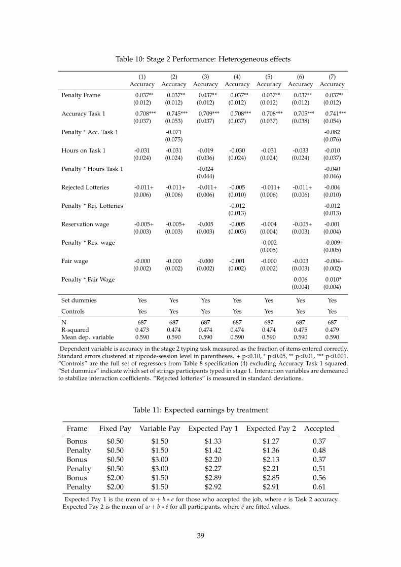
Table 10: Stage 2 Performance: Heterogeneous effects

(1) (2) (3) (4) (5) (6) (7)Accuracy Accuracy Accuracy Accuracy Accuracy Accuracy Accuracy

Penalty Frame 0.037** 0.037** 0.037** 0.037** 0.037** 0.037** 0.037**(0.012) (0.012) (0.012) (0.012) (0.012) (0.012) (0.012)

Accuracy Task 1 0.708*** 0.745*** 0.709*** 0.708*** 0.708*** 0.705*** 0.741***(0.037) (0.053) (0.037) (0.037) (0.037) (0.038) (0.054)

Penalty * Acc. Task 1 -0.071 -0.082(0.075) (0.076)

Hours on Task 1 -0.031 -0.031 -0.019 -0.030 -0.031 -0.033 -0.010(0.024) (0.024) (0.036) (0.024) (0.024) (0.024) (0.037)

Penalty * Hours Task 1 -0.024 -0.040(0.044) (0.046)

Rejected Lotteries -0.011+ -0.011+ -0.011+ -0.005 -0.011+ -0.011+ -0.004(0.006) (0.006) (0.006) (0.010) (0.006) (0.006) (0.010)

Penalty * Rej. Lotteries -0.012 -0.012(0.013) (0.013)

Reservation wage -0.005+ -0.005+ -0.005 -0.005 -0.004 -0.005+ -0.001(0.003) (0.003) (0.003) (0.003) (0.004) (0.003) (0.004)

Penalty * Res. wage -0.002 -0.009+(0.005) (0.005)

Fair wage -0.000 -0.000 -0.000 -0.001 -0.000 -0.003 -0.004+(0.002) (0.002) (0.002) (0.002) (0.002) (0.003) (0.002)

Penalty * Fair Wage 0.006 0.010*(0.004) (0.004)

Set dummies Yes Yes Yes Yes Yes Yes Yes

Controls Yes Yes Yes Yes Yes Yes Yes

N 687 687 687 687 687 687 687R-squared 0.473 0.474 0.474 0.474 0.474 0.475 0.479Mean dep. variable 0.590 0.590 0.590 0.590 0.590 0.590 0.590

Dependent variable is accuracy in the stage 2 typing task measured as the fraction of items entered correctly.Standard errors clustered at zipcode-session level in parentheses. + p<0.10, * p<0.05, ** p<0.01, *** p<0.001.“Controls” are the full set of regressors from Table 8 specification (4) excluding Accuracy Task 1 squared.“Set dummies” indicate which set of strings participants typed in stage 1. Interaction variables are demeanedto stabilize interaction coefficients. “Rejected lotteries” is measured in standard deviations.

Table 11: Expected earnings by treatment

Frame Fixed Pay Variable Pay Expected Pay 1 Expected Pay 2 Accepted

Bonus $0.50 $1.50 $1.33 $1.27 0.37Penalty $0.50 $1.50 $1.42 $1.36 0.48Bonus $0.50 $3.00 $2.20 $2.13 0.37Penalty $0.50 $3.00 $2.27 $2.21 0.51Bonus $2.00 $1.50 $2.89 $2.85 0.56Penalty $2.00 $1.50 $2.92 $2.91 0.61

Expected Pay 1 is the mean of w + b ∗ e for those who accepted the job, where e is Task 2 accuracy.Expected Pay 2 is the mean of w + b ∗ e for all participants, where e are fitted values.

39

Appendices

A Model extensions

In the basic model I assume no diminishing sensitivity (i.e. utility is linear except for akink at the reference point), that the reference point is entirely determined by P’s choiceof frame, and that there is no loss aversion in effort choice. In this appendix I discusseach of these candidate extensions in turn.

A.1 Diminishing sensitivity

Suppose that A’s gain-loss utility exhibits diminishing sensitivity, à la Kahneman andTversky (1979). Specifically, it is concave in the gain domain and convex in the lossdomain. I assume that gain-loss utility for consumption x and reference point r equalsµ(x − r) if x ≥ r and −λµ(x − r) if x < r, where µ(.) is a concave function. Forsimplicity I assume consumption utility is still linear. The utility function (1) becomes:

U(e, w, b, F) = w + eb−(

e2

2γ− αe

)+ eµ((1− F)b)− λ(1− e)µ(Fb) (8)

Notice first that A’s utility is still decreasing in F, since a higher reference pointmakes her worse off in every state of the world. Therefore firms will still tend to shyaway from penalties, as in Proposition 1.

As for the choice of effort, it is slightly more complex than before. I obtain:

e∗(w, b, F) = γ[α + b + µ((1− F)b) + λµ(Fb)]de∗

dF= γb[λµ′(Fb)− µ′((1− F)b)].

It is no longer guaranteed that e∗ is increasing in F. de∗dF > 0 ↔ λ > µ′((1−F)b)

µ′(Fb) , whichwill fail in the neighborhood of F = 1 if µ is sufficiently steep at zero. Intuitively,there are opposing effects to increasing the reference point: it makes A feel more dis-appointed when unsuccessful, but less elated when successful. Diminishing sensitivityimplies that eventually the latter may outweigh the former, reducing effort, and furtherdiscouraging the use of penalties. Note however that d2e∗

dFdλ > 0 as before, i.e. penaltieshave a stronger effect on more loss-averse people.

A.2 Reference-dependent effort provision

Crawford and Meng (2011) argue that reference dependence in effort provision maybe an important determinant of labor supply, and that taxi drivers exhibit behaviorconsistent with both income and hours targeting. To capture this in a simple way,assume that A has an effort target er, and is pleased when actual effort is below thetarget level, and displeased when above.

40

The key question in this context is what effect the choice of monetary frame has onthe effort target. If, as in Crawford and Meng (2011), A simply has an exogenous efforttarget, then the main results go through essentially unchanged. If the penalty framedecreases A’s effort target then penalty framing will reduce her utility by even morethan before. Lastly if the frame increases her target, it can actually be the case that thepenalty frame increases her utility. The reduction of the loss (increase in the gain) ingain-loss utility over effort can offset the increase in loss (decrease in gain) of gain-lossutility over consumption.

I choose not to push this mechanism as a possible explanation for the main findingthat penalties are more popular than bonuses, simply because I feel there is no a priorireason to think that a penalty frame over payoff outcomes would increase or decreasethe effort target, and in particular that this effect would dominate the effect of loss aver-sion over consumption, which is the domain specifically targeted by the intervention.41

I assume that gain-loss utility in effort enters linearly, weighted by a parameterη. Note that since effort is a non-stochastic choice, A will be either always above,always below or exactly at her effort target. I assume that gain-loss disutility in effort isλη(e− er) when e ≥ er and (e− er) when e < er. A’s utility function is now:

U(e, w, b, F) = w + e[α + b(2 + (λ− 1)F)]− λFb− e2

2γ

− η(e− er)(λ(1− 1[e < er]) + 1[e < er])

(9)

Differentiating U with respect to F yields ∂U∂F = eb(λ− 1)− λb + η der

dF (λ(1− 1[e <

er]) + 1[e < er]). Apart from the discontinuity at e = er, this expression is maximizedat e = 1 ≥ er, equal to −b + ηλ der

dF . Overall the sign on the expression is ambiguous,particularly since I lack a theory of how er depends on b and F.

A’s optimal effort choice is as follows:

e∗(w, b, F) =

eH eH ≤ er

er eL < er < eH

eL er ≤ eL

where eH = γ[α + b(2 + (λ− 1)F]− η], and eL = γ[α + b(2 + (λ− 1)F]− ηλ].Notice first that both eH and eL are increasing in F at rate γbλ. Therefore a) if er is

increasing in F, then e∗ is everywhere increasing in F; b) if er does not depend on F,then e∗ is increasing in F for eH < er or eL > er and flat when eL < er < eH, and lastly c)if er is decreasing in F, then e∗ is first increasing, then decreasing, then increasing again.

41Moreover, a reasonable model for the setting of effort targets would be KR, such that the target isexpected effort. However since effort is non-stochastic, expected and actual effort will always coincide sothe gain-loss over effort term drops out altogether.

41

A.3 Expectations-based reference point (KR)

In the basic model I assume that the reference point is entirely determined by P’s frame.However, KR argue that in many contexts it makes sense to think of expectations as anatural reference point. In this section I outline how to incorporate this intuition intothe model.

In KR, the reference point is the expected distribution of outcomes. For example,an agent holding a lottery ticket that pays $50 with 50% probability has a stochasticreference point that equals $50 with probability one half and $0 with probability onehalf. The most natural specification of the reference point in work on moral hazardunder loss aversion applies Koszegi and Rabin (2007)’s concept of choice-acclimatingpersonal equilibrium (CPE).42 Under CPE, the agent’s choices influence her referencepoint, and she takes account of this effect when making her decision, i.e. her referencepoint and choices are simultaneously determined. For instance, under CPE, an agentknows that buying a lottery ticket will increase her expected winnings, which will beincorporated into her reference point. This creates the possibility of experiencing a losswhen she does not win, which might ultimately lead her not to purchase a ticket. Inthe moral hazard context, higher effort leads to a higher chance of receiving b, whichincreases the reference point, and the agent anticipates this when choosing her effortlevel.

I continue to ignore risk aversion in the conventional sense, as well as diminishingsensitivity. I continue to assume that equal weight is placed on consumption and gain-loss utility (i.e. KR’s η parameter equals one), and I continue to assume no loss aversionover effort choice. Formally, for reference point r distributed according to H(r|e, F) A’sutility function becomes:

U(G|H, e, F) = w + eb− e2

2γ+ αe︸ ︷︷ ︸

Consumption and effort cost

+ e∫

µ(w + b− r)dH(r|e, F) + (1− e)∫

µ(w− r)dH(r|e, F)︸ ︷︷ ︸Gain-loss utility

.(10)

Where as before µ(x− r) equals x− r if x ≥ r and λ(x− r) if x < r.In KR, the reference point is determined by recently held expectations, and in par-

ticular there is no mechanism for it to be influenced by framing. To allow for framingeffects in the simplest possible way, I assume the reference point takes the form ofa weighted sum of the KR reference point and the frame supplied by the principal.

42This is the specification used by Gill and Prowse (2012) and Herweg et al. (2010).

42

Formally, the marginal distribution of r is:

h(x|e, F) = Pr(r = x|e, F) =

1− e x = φw + (1− φ)(w + Fb)

e x = φ(w + b) + (1− φ)(w + Fb)(11)

F ∈ [0, 1], φ ∈ [0, 1).

As before, w + Fb is the “base pay” supplied as a reference point by the principal, andF corresponds to the fraction of the bonus b that is presented as part of the base pay.F = 0 is a pure bonus frame with base pay w; F = 1 is a pure penalty frame with basepay w + b. φ captures how susceptible the agent is to framing effects. φ = 1 coincideswith KR’s model, in which framing has no effect on behavior. φ = 0 corresponds to thebasic model in the text. For intermediate values of φ, A’s reference point lies in betweenw and w + b and she experiences mixed emotions whether she receives or does notreceive the bonus.

Incorporating the above assumptions, A’s gain-loss utility sums over four states ofthe world. With probability e2, her consumption is w + b and her reference point isφ(w + b) + (1− φ)(w + Fb) ≤ w + b, putting her in the gain domain. With probabilitye(1− e) her consumption is w + b and her reference point is φw + (1− φ)(w + Fb) ≤w + b, again putting her in the gain domain. With probability e(1− e) her consumptionis w and her reference point is φ(w + b) + (1− φ)(w + Fb) ≥ w, putting her in the lossdomain, and with probability (1− e)2 her consumption is w and her reference point isφw + (1− φ)(w + Fb) ≥ w, again putting her in the loss domain. Plugging these into(10) and simplifying, I can write her utility as:

U(e, w, b, F) = e[α + b((2− λφ) + (λ− 1)(1− φ)F)]− e2[

12γ− (λ− 1)φb

]+ w− λ(1− φ)Fb.

(12)

A.3.1 Effort choice

Suppose A accepts the contract. I impose two parameter restrictions that are sufficientfor the optimal equilibrium effort choice to be interior (i.e. lie in the interval (0, 1)) andgiven by the first-order condition.

Assumption 1 No dominance of gain-loss utility: λ < 2φ ≡ λ.

Assumption 2 No top-coding in effort: γ < γ ≡ 1α+v[1+λ−φ]

.

43

Under Assumptions 1 and 2, A’s optimal effort choice is equal to:43

e∗(b, F) =γ[α + b((2− λφ) + (λ− 1)(1− φ)F)]

1− 2γ(λ− 1)φb(13)

Assumption 1 ensures that A is not so strongly loss averse that she is discouragedfrom exerting any effort at all. This can happen because her reference point is increasingin her effort choice, as higher effort increases her expected earnings. Intuitively, ifλ is large, the increase in her disappointment when unsuccessful outweighs the higherexpected earnings, such that she prefers to not to exert any effort. Assumption 2 simplyensures e∗ < 1.

It is easy to see that the three predictions of the basic model go through: effort isincreasing in F, more strongly so for more loss-averse agents. A’s utility is decreasingin F (just apply the envelope theorem to (12)), so Proposition 1 will hold.

The key difference now is that it is possible for effort to be decreasing in λ, as I findin the experiment. Differentiating e∗ with respect to λ yields:

de∗

dλ=

γb[(1− φ)F− φ(1− 2γ(α + b(2− φ)))]

(1− 2γ(λ− 1)φb)2 (14)

The sign of this expression is ambiguous. In particular, suppose F = 0. Then de∗dλ is

negative if φ > 0 and 1 > 2γ(α + b(2− φ)).The intuition for this finding is the feedback between effort and the reference point

in the model. On the one hand, increasing effort reduces the probability of experiencinga loss. On the other hand, as A increases her effort, she also increases her referencepoint, and thus the size of the loss when unsuccessful. It may that the latter effectoutweighs the former, and hence that effort can be decreasing in λ. Note, however, thatthis does not change the prediction that the positive effect of incentive framing on effortis stronger for more loss-averse agents.

43To see that Assumptions 1 and 2 imply that e∗ is the unique, interior maximizer of (12), first notethat the second order condition can be written as 2γ(λ− 1)φb < 1. Assuming this holds, we have e∗ > 0for all F, α and b > 0, provided 2− λφ > 0, which is Assumption 1. Second, e∗ < 1 for all F, α providedγb[(2−λφ)+ (λ− 1)(1−φ)+ 2(λ− 1)φ] < 1, which can be easily seen to imply the second order conditionwhen Assumption 1 holds, and therefore sufficiency of the first-order condition. Last, note that non-negative profits imply b ≤ v, so substituting v for b and simplifying, the expression reduces to Assumption2, which is therefore sufficient for e∗ < 1 in equilibrium. Assumption 1 is the analog of the assumption ofthe same name in Herweg et al. (2010), whose model corresponds to the case φ = 1.

44

B Additional Results

B.1 Summary distributions

0

.05

.1

.15

.2

Den

sity

0 3 6 9 12Rejected Lotteries

0

.05

.1

.15

.2

.25

Den

sity

0 5 10 15Reservation wage, $/hr

0

.05

.1

.15

.2

.25

Den

sity

0 5 10 15Minimum fair wage, $/hr

0

.5

1

1.5

2

Ker

nel d

ensi

ty e

stim

ate

0 .2 .4 .6 .8 1Accuracy rate

0

.2

.4

.6

Ker

nel d

ensi

ty e

stim

ate

-8 -6 -4 -2 0Log distance measure (errors per item)

0

.5

1

1.5

2

Ker

nel d

ensi

ty e

stim

ate

0 .5 1 1.5 2 2.5Time spent, hours

Stage 1 Stage 2

Figure B.1: Distributions of survey responses and task performance. Reservation wage,fair wage and time spent trimmed at the 99th percentile (minimum acceptable wage =$10, minimum fair wage = $14, time = 1.75 hours (round 1), 2.65 hours (round 2)).

45

B.2 Relation between stage 1 variables.

Before analyzing stage 2 behavior, it is instructive to analyze the relationships betweenthe key variables measured in stage 1. The main variables of interest are the accuracyscore, time spent on the effort task, the number of rejected lotteries, the reservationwage and the minimum fair wage reported by each participant. Table B.1 reports cor-relations between these variables with and without dropping participants who madeinconsistent lottery choices. Higher performance on the stage 1 task is significantlynegatively correlated with time spent on the task. Reservation wage and minimum fairwage are strongly positively correlated with one another. Reservation wage is nega-tively correlated with time spent on task 1, but not with performance. Lastly, there isno economically or statistically significant correlation between reservation wages, thenumber of rejected lotteries, and performance on the first stage task (rejected lotteriesare significantly positively correlated with performance, but only when including par-ticipants who made inconsistent choices). These results suggest that selection on, say,loss aversion, will not necessarily imply selection on ability.

Table B.2 regresses stage 1 performance on various key variables. Time spent onstage 1 is robustly negatively correlated with performance on the effort task, with eachadditional hour spent associated with around 10 percentage points lower accuracy. Un-like the simple correlations, the minimum acceptable wage is now robustly negativelyrelated with performance, perhaps because participants with higher reservation wagesmay be more likely to rush the task and therefore make more errors. A 1s.d. increasein the minimum acceptable wage ($2.70) is associated with 1.5-2.5 percentage pointslower accuracy. In one specification, the minimum fair wage is positively associatedwith accuracy, controlling for reservation wages. Lastly, the number of rejected lotteriesis positively associated with performance, although this is not statistically significantwhen participants who made inconsistent choices are dropped. The coefficient esti-mates imply a 0.6 to 1.3 percentage point improvement for a 1s.d. increase in thenumber of rejected lotteries.

Of the other variables, higher weekly Mturk earnings are negatively associated withperformance, (although higher hours on MTurk positively associated, perhaps becausethose higher earnings are attained by expending less effort on each individual task).Participants who report that they mainly work on MTurk to earn money (93% of partic-ipants, other options “for fun”, “other”) perform around 5-6 percentage points better,men perform around four percentage points better, and participants who made incon-sistent lottery choices around 8 percentage points worse.

46

Table B.1: Correlation between key stage 1 variables

Panel A

Accuracy T1 Hours on T1 Rej. lotteries Res. wage Fair wage

Accuracy T1 1Hours on T1 -0.174*** 1Rej. lotteries 0.0678** -0.0275 1Res. wage -0.0403 -0.107*** -0.0864*** 1Fair wage -0.00588 -0.0426 -0.0446 0.513*** 1

Observations 1450

Panel B

Accuracy T1 Hours on T1 Rej. lotteries Res. wage Fair wage

Accuracy T1 1Hours on T1 -0.173*** 1Rej. lotteries 0.0429 -0.0160 1Res. wage -0.0348 -0.114*** -0.0786** 1Fair wage 0.00456 -0.0414 -0.0386 0.507*** 1

Observations 1351

Correlation matrices. * p<0.05, ** p<0.01, *** p<0.001. Accuracy T1 is accuracy on thestage 1 typing task. Hours on T1 is the median time spent on a page of the stage 1 task,multiplied by 10. Panel A includes all participants, Panel B drops participants who madeinconsistent lottery choices.

47

Table B.2: Performance on stage 1

(1) (2) (3) (4)Accuracy Accuracy Accuracy Accuracy

Hours on Task 1 -0.107*** -0.131*** -0.096***(0.015) (0.022) (0.018)

Rejected Lotteries 0.009* 0.006 0.011* 0.013**(0.005) (0.005) (0.005) (0.005)

Reservation wage -0.005* -0.009** -0.005** -0.005*(0.002) (0.003) (0.002) (0.002)

Fair wage 0.002 0.006* 0.002 0.002(0.002) (0.003) (0.003) (0.003)

Session 2 -0.020+ -0.017 -0.022+ -0.022+(0.011) (0.013) (0.012) (0.012)

Hours working on MTurk per week 0.001 0.000(0.000) (0.000)

Typical MTurk earnings, $100/week -0.017+ -0.017+(0.009) (0.009)

MTurk HITs completed -0.000 -0.000(0.000) (0.000)

Months of experience on MTurk 0.000 0.000(0.000) (0.000)

Mainly participate in research HITs 0.002 -0.002(0.011) (0.011)

Work on MTurk mainly to earn money 0.051** 0.057**(0.019) (0.020)

Age -0.000 -0.001(0.001) (0.001)

Male 0.037*** 0.038***(0.010) (0.010)

Inconsistent Lottery Choices -0.078*** -0.084***(0.017) (0.017)

Constant 0.549*** 0.562*** 0.391*** 0.337***(0.021) (0.025) (0.057) (0.057)

Set dummies Yes Yes Yes Yes

Controls No No Yes Yes

N 1448 1147 1447 1449R-squared 0.053 0.056 0.107 0.082Mean of dependent variable 0.456 0.463 0.456 0.455

Dependent variable is accuracy rate on stage 1 typing task. Standard errors clustered atzipcode-session level in parentheses. + p<0.10, * p<0.05, ** p<0.01, *** p<0.001. All columnsinclude dummies for the set of items typed. Column (2) drops participants who made in-consistent lottery choices, and those above the 99th percentile for time spent, reservationwage and fair wage. “Controls” are dummy variables for income, education and employ-ment status. Rejected lotteries measured in standard deviations.

48

B.3 Balance checks

0

.2

.4

.6

.8

1

Cum

ulat

ive

dens

ity

0 .2 .4 .6 .8 1Accuracy Rate Task 1

0

.2

.4

.6

.8

1

Cum

ulat

ive

dens

ity

0 3 6 9 12Rejected Lotteries

0

.2

.4

.6

.8

1

Cum

ulat

ive

dens

ity

0 3 6 9 12Reservation Wage, $/hr

0

.2

.4

.6

.8

1

Cum

ulat

ive

dens

ity

0 3 6 9 12Fair Wage, $/hr

Bonus

Penalty

Figure B.2: Balance between bonus and penalty treatments, all incentive levels. Reser-vation wage (minimum acceptable wage) trims at the 99th percentile.

B.4 Comparing Session 1 and 2 Participants

0

.2

.4

.6

.8

1

Cum

ulat

ive

dens

ity

0 .2 .4 .6 .8 1Accuracy Rate Task 1

0

.2

.4

.6

.8

1

Cum

ulat

ive

dens

ity

0 3 6 9 12Rejected Lotteries

0

.2

.4

.6

.8

1

Cum

ulat

ive

dens

ity

0 3 6 9 12Reservation Wage, $/hr

0

.2

.4

.6

.8

1

Cum

ulat

ive

dens

ity

0 3 6 9 12Fair Wage, $/hr

Session 1

Session 2

Figure B.3: Comparing session 1 and 2 participants. Reservation wage (minimum ac-ceptable wage) trims at the 99th percentile.

49

B.5 Selection: Robustness

Table B.3: Selection: Robustness

(1) (2) (3) (4)Accepted Accepted Accepted Accepted

Penalty Frame 0.108*** 0.102*** 0.102*** 0.105***(0.026) (0.027) (0.026) (0.026)

Accuracy Task 1 0.286*** 0.281*** 0.278*** 0.289***(0.076) (0.078) (0.076) (0.076)

Hours on Task 1 -0.182** -0.180*** -0.173*** -0.174***(0.069) (0.046) (0.043) (0.044)

Penalty * Hours Task 1 0.018(0.097)

Rejected Lotteries 0.004 0.013 0.002 0.005(0.013) (0.019) (0.013) (0.013)

Penalty * Rej. Lotteries -0.021(0.026)

Reservation wage -0.016** -0.013** -0.033*** -0.015**(0.005) (0.005) (0.009) (0.005)

Penalty * Res. wage 0.021+(0.012)

Fair wage 0.005 0.003 0.004 -0.007(0.006) (0.006) (0.006) (0.009)

Penalty * Fair Wage 0.014(0.012)

Set dummies Yes Yes Yes Yes

Controls Yes Yes Yes Yes

N 1433 1348 1433 1433R-squared 0.113 0.114 0.117 0.115Mean dep. variable 0.477 0.481 0.473 0.472

Dependent variable is a dummy indicating whether the participant ac-cepted the job offer in stage 2. Estimates from OLS linear probability model.Standard errors clustered at zipcode-session level in parentheses. + p<0.10,* p<0.05, ** p<0.01, *** p<0.001. Column (1) drops participants above the99th percentile of time spent on task 1. Column (2) drops those who madeinconsistent lottery choices. Column (3) drops participants above the 99thpercentile of reservation wage. Column (4) drops participants above the99th percentile of fair wage. “Controls” are the full set of regressors fromTable 5 specification (4) excluding Accuracy Task 1 squared. “Set dummies”indicate which set of strings participants typed in stage 1. Interaction vari-ables are demeaned in each specification to stabilize interaction coefficients.“Rejected lotteries” is measured in standard deviations.

50

B.6 Alternative performance and effort measure

Table B.4: Performance/effort on stage 2, alternative measures

(1) (2) (3) (4)Log distance Log distance Time spent Time spent

Penalty Frame -0.205* -0.209** 0.054* 0.028(0.090) (0.080) (0.027) (0.023)

High Fixed Pay -0.251* -0.323** 0.013 0.023(0.119) (0.113) (0.036) (0.031)

High Variable Pay -0.048 -0.069 0.026 0.036(0.133) (0.130) (0.040) (0.033)

Accuracy Task 1 0.152(0.384)

Accuracy Task 1 ^2 -0.084(0.382)

Log Errors per item Task 1 0.868***(0.066)

Hours on Task 1 0.735***(0.067)

Rejected Lotteries 0.036 -0.018(0.040) (0.012)

Reservation wage 0.025 0.001(0.021) (0.006)

Fair wage -0.010 -0.001(0.020) (0.005)

Session 2 0.160 0.031 0.006 -0.035(0.149) (0.127) (0.046) (0.036)

Inconsistent Lottery Choices 0.305 -0.036(0.189) (0.042)

Set dummies Yes Yes Yes Yes

Controls No Yes No Yes

N 687 687 680 680R-squared 0.075 0.338 0.029 0.400Mean dep. variable -3.825 -3.825 0.687 0.687

Dependent variable in columns (1) and (2) is the log of the mean scaled Levenshtein distance (which can beinterpreted as the mean number of errors per character in the typing task). Dependent variable in columns(3) and (4) is time spent on the stage 2 typing task, estimated as 10 times the median time spent per pageof typed items, in addition dropping participants above the 99th percentile for time spent. Standard errorsclustered at zipcode-session level in parentheses. + p<0.10, * p<0.05, ** p<0.01, *** p<0.001. “Set dummies”indicate which set of strings participants typed in stages 1 and 2. “Controls” are Hours worked on MTurkper week, MTurk earnings per week, HITs completed, MTurk experience, “Mostly do research HITs”,“Mainly MTurk to earn money”, age, male, and income, occupation and education dummies. “Rejectedlotteries” is measured in standard deviations.

51

B.7 Participants’ predictions of Task 1 accuracy

Table B.5: Participants’ Predictions of stage 1 Accuracy

(1) (2) (3) (4)Predicted Acc. Predicted Acc. Accuracy Accuracy

Penalty Frame 0.002 0.001 0.036* 0.036**(0.015) (0.014) (0.015) (0.012)

High Fixed Pay 0.006 0.010 0.022 0.037*(0.020) (0.019) (0.020) (0.017)

High Variable Pay 0.033 0.036+ 0.006 0.024(0.020) (0.020) (0.021) (0.019)

Session 2 -0.040+ -0.035 -0.030 -0.017(0.022) (0.022) (0.024) (0.019)

Predicted Acc. 0.201*** -0.006(0.040) (0.032)

Set dummies Yes Yes Yes Yes

Controls No Yes No Yes

N 686 686 686 686R-squared 0.022 0.150 0.094 0.476Mean of dependent variable 0.577 0.577 0.590 0.590

Dependent variable in (1) and (2) is participant’s prediction of mean stage 1 accuracy, andin (3) and (4) is participant’s actual stage 2 accuracy. Standard errors clustered at zipcode-session level in parentheses. + p<0.10, * p<0.05, ** p<0.01, *** p<0.001.“Set dummies” indicate which set of strings participants typed in stage 1 (column (2))

or stages 1 and 2 (column (4)). “Controls” are the full set of regressors from the mainspecifications.

52

B.8 Comparing sessions 1 and 2

Table B.6: Comparing Sessions 1 and 2

(1) (2) (3) (4) (5) (6) (7) (8)Accepted Accepted Accuracy Accuracy Log distance Log distance Time spent Time spent

Penalty 0.156** 0.137** 0.037 0.039+ -0.317+ -0.238 0.051 0.040(0.052) (0.052) (0.029) (0.023) (0.186) (0.168) (0.055) (0.049)

Session 2 -0.007 -0.015 -0.020 -0.000 -0.032 -0.062 -0.043 -0.061(0.053) (0.053) (0.039) (0.030) (0.242) (0.198) (0.057) (0.052)

Penalty * Session 2 -0.038 0.006 -0.029 -0.028 0.330 0.149 0.089 0.045(0.076) (0.075) (0.051) (0.038) (0.308) (0.256) (0.087) (0.071)

Set dummies No Yes No Yes No Yes No Yes

Controls No Yes No Yes No Yes No Yes

N 688 1447 302 687 302 687 300 680R-squared 0.021 0.115 0.012 0.477 0.013 0.343 0.017 0.402Mean dep. variable 0.439 0.475 0.580 0.590 -3.729 -3.825 0.698 0.687

This table compares outcomes between treatment groups 2 and 3 (session 1) with groups 6 and 7 (session 2). Each received thesame economic incentives (fixed pay of $0.50 and variable pay of $3.00), but the job offer was rephrased in session 2 to explorewhether inattention might explain the session 1 results. Dependent variable in columns (1) and (2) is a dummy indicating whetherthe participant accepted the job offer in stage 2; in columns (3) and (4) is the participant’s accuracy score in stage 2; in columns (5)and (6) is the “distance” accuracy measure described in table B.4 and in columns (7) and (8) is the time spent by the participanton the task in stage 2. Columns (7) and (8) drop participants above the 99th percentile of time spent. Standard errors clustered atzipcode-session level in parentheses. + p<0.10, * p<0.05, ** p<0.01, *** p<0.001. Odd-numbered columns do not include controls anduse data from groups 2, 3, 6 and 7. Even-numbered columns include the full sets of controls from the equivalent main specifications,and use data from all participants to increase precision of estimated coefficients on control variables, differencing out the maineffects for treatment groups 0, 1, 4 and 5 using dummy variables.

53

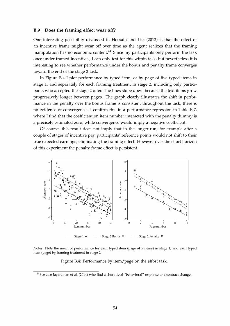
B.9 Does the framing effect wear off?

One interesting possibility discussed in Hossain and List (2012) is that the effect ofan incentive frame might wear off over time as the agent realizes that the framingmanipulation has no economic content.44 Since my participants only perform the taskonce under framed incentives, I can only test for this within task, but nevertheless it isinteresting to see whether performance under the bonus and penalty frame convergestoward the end of the stage 2 task.

In Figure B.4 I plot performance by typed item, or by page of five typed items instage 1, and separately for each framing treatment in stage 2, including only partici-pants who accepted the stage 2 offer. The lines slope down because the text items growprogressively longer between pages. The graph clearly illustrates the shift in perfor-mance in the penalty over the bonus frame is consistent throughout the task, there isno evidence of convergence. I confirm this in a performance regression in Table B.7,where I find that the coefficient on item number interacted with the penalty dummy isa precisely estimated zero, while convergence would imply a negative coefficient.

Of course, this result does not imply that in the longer-run, for example after acouple of stages of incentive pay, participants’ reference points would not shift to theirtrue expected earnings, eliminating the framing effect. However over the short horizonof this experiment the penalty frame effect is persistent.

.3

.4

.5

.6

.7

.8

.9

Acc

urac

y ra

te

0 10 20 30 40 50Item number

.3

.4

.5

.6

.7

.8

.9

Acc

urac

y ra

te

0 2 4 6 8 10Page number

Stage 1 Stage 2 Bonus Stage 2 Penalty

Notes: Plots the mean of performance for each typed item (page of 5 items) in stage 1, and each typeditem (page) by framing treatment in stage 2.

Figure B.4: Performance by item/page on the effort task.

44See also Jayaraman et al. (2014) who find a short lived “behavioral” response to a contract change.

54

Table B.7: Performance by item in effort task

(1)Item correct

Penalty Frame 0.038**(0.014)

Item 0.006***(0.002)

Item x Penalty 0.000(0.000)

Set dummies Yes

Page dummies Yes

Controls Yes

N 34350R-squared 0.126Mean of dependent variable 0.590

Dependent variable is a dummy indicating whether an item was entered correctly. Standarderrors clustered at zipcode-session level in parentheses. + p<0.10, * p<0.05, ** p<0.01, ***p<0.001. “Set dummies” indicate sets of strings participants typed in stage 1 and 2. “Pagedummies” indicate the page of the current item. “Controls” are the full set of regressors fromthe main specifications, plus High Fixed and High Variable pay dummies.

B.10 Standard Selection Effect

In this section I briefly show that I do find a standard selection effect: that higher abilityworkers are more likely to accept the stage 2 offers of incentive pay, as also found byLazear (2000) and Dohmen and Falk (2011), for example.

Figure B.1 shows the distribution of accuracy measures in stages 1 and 2, showinga large increase in performance in stage 2. This increase depends on three things: theeffect of incentive pay on effort, the effect of incentive pay on selecting in motivated orable workers, and learning by doing. I cannot separate out learning by doing since I donot have a flat pay incentive treatment in stage 2, however I can illustrate the effect ofselection.

Figure B.5 plots CDFs of stage 1 variables, comparing acceptors with rejectors (pool-ing all treatments). Acceptors performed better in stage 1, spent less time, and havelower reservation and fair wages, each one suggesting a first-order stochastic domi-nance shift. As previously noted I see little difference in rejected lotteries, which issurprising since the incentive pay is inherently risky. The differences in ability arealso demonstrated by comparing stage 1 performance measures between acceptors andrejectors in Table 2

Ideally, to demonstrate the selection effect on performance I would regress accuracyon a “round 2” dummy, with and without controlling for ability. This is not possiblesince my main ability measure is performance on the stage 1 task, which is also an

55

outcome.45 Instead, I perform the following simple exercise. I assume that the true per-formance model is linear and equal to that estimated in Table 8 column (4) (excludingthe “set” dummy variables for the stage 2 task, since these are only observed for thosewho performed the task). Using this model I impute task 2 accuracy for rejectors.

The results are as follows. Mean accuracy across all participants in stage 1 is equalto 0.46, while in stage 2 it is equal to 0.59. Ignoring selection, a naive estimate of thecombined effect of learning by doing and incentive pay would therefore be equal to a13 percentage point improvement. However, the mean fitted stage 2 accuracy for allparticipants, including rejectors, is 0.56. Under the strong assumption that the fittedmodel is the true model, this implies that three percentage points of the combinedeffect can be attributed to advantageous selection of workers into incentive pay. Analternative way to control for selection is to compare mean performance of acceptors instage 2 with mean performance of acceptors in stage 1, equal to 0.48. This gives me asimilar effect of incentives and learning equal to 11 percentage points.

45Furthermore, I do not have a variable that will plausibly satisfy the exclusion restriction needed for aselection model.

56

0

.2

.4

.6

.8

1

Cum

ulat

ive

dens

ity

0 .2 .4 .6 .8 1Accuracy Rate Task 11, percent

0

.2

.4

.6

.8

1

Cum

ulat

ive

dens

ity

0 .5 1 1.5 2Time Spent Task 1, hours

0

.2

.4

.6

.8

1

Cum

ulat

ive

dens

ity

0 3 6 9 12Rejected Lotteries

0

.2

.4

.6

.8

1

Cum

ulat

ive

dens

ity

0 3 6 9 12Reservation Wage, $/hr

0

.2

.4

.6

.8

1

Cum

ulat

ive

dens

ity

0 3 6 9 12Fair Wage, $/hr

Rejected Accepted

Figure B.5: Comparing Acceptors vs Rejectors. Reservation and fair wage trimmed atthe 99th percentile.

57

B.11 Participant locations

Participant locations

Figure B.6: Participant locations by geocoded zipcodes

58

B.12 Follow-up survey

Table B.8: Participants’ perceptions of the job offer they received

Panel A

The job offer or task is...

(1) (2) (3) (4) (5) (6) (7) (8)Fun Easy Good pay Fair Good motivator Trustworthy Achievable Understandable

Penalty -0.091 -0.104 0.295* -0.171 -0.138 -0.045 -0.204+ -0.155(0.121) (0.126) (0.121) (0.123) (0.128) (0.126) (0.121) (0.128)

Accepted offer 0.481*** 0.366** 0.592*** 0.658*** 0.697*** 0.523*** 0.763*** 0.241+(0.128) (0.140) (0.141) (0.134) (0.139) (0.139) (0.131) (0.139)

N 252 252 252 252 252 252 252 252R-squared 0.286 0.198 0.260 0.279 0.257 0.250 0.280 0.155

Panel B

Offer attractive because... Offer unattractive because...

(1) (2) (3) (4) (5) (6)Good pay Elated if receive $3.50 Encourages effort Risky Disappointed if receive $0.50 Difficult

Penalty 0.304* 0.232+ -0.108 -0.078 0.170 0.089(0.124) (0.126) (0.128) (0.115) (0.116) (0.114)

Accepted offer 0.627*** 0.437** 0.699*** -0.882*** -0.778*** -0.924***(0.142) (0.147) (0.138) (0.129) (0.126) (0.131)

N 252 252 252 252 252 252R-squared 0.276 0.219 0.275 0.358 0.328 0.316

Panel C

Estimated aggregate behavior

(1) (2)Est. acceptance rate Est. success rate

Penalty -0.006 -0.014(0.032) (0.037)

Accepted offer 0.202*** 0.118**(0.035) (0.043)

N 252 252R-squared 0.321 0.179Mean dep. variable 0.560 0.446

Standard errors clustered at zipcode level in parentheses. + p<0.10, * p<0.05, ** p<0.01, *** p<0.001. Dependent variablesin Panels A and B are standardized measures of agreement, measured on a 1-7 scale. Panel C asked participants toestimate the fraction of participants who received the same job offer as themselves and accepted, and the performance ofacceptors. All regressions include the full set of controls from the main specifications.

59

C Experimental details

C.1 Rates of pay

One potential concern about the study is the low size of the incentives used: the max-imum a participant could earn in stage 1 is $3 and the maximum in stage 2 is $3.50. Ifa participant spent 30 minutes on stage 1 this implies a $6 hourly wage, significantlylower than the typical rates of pay in experimental labs, for example. The size of theincentive was selected, based on trial runs of the task, to match Amazon’s suggestedrate of pay of $6; the concern was that paying more would be perceived as unusual ornot comparable to other jobs on MTurk. More critically, to study selection effects it iscritical that rates of pay are low enough that some participants do not want to acceptthe job. The 47% acceptance rate in stage 2 suggests that rates were pitched about right.Taking into account the level of the incentives, the relative sizes of the fixed and variablepay in stage 2 were selected to be reasonably high-powered to emphasize the role of thepenalty component of the contract.

C.2 Accuracy report after first stage

Shortly after the first stage was completed, subjects were sent an email informing themof their performance. The purpose of this was to ensure that they understood thedifficulty level of the task and had at least a sense of their ability. An example messageis given below:

Thanks for doing the typing task + survey HIT.

We have now processed the data and approved your work. We estimate

that out of the 50 items, you entered 31 (62%) without errors.

Best wishes

Jon

C.3 Invitation to second stage

C.3.1 Session 1

One week after the first stage, all participants from the first stage were sent a secondemail inviting them to the second stage task under their randomly assigned incentive.

Thanks for participating in our recent typing task and survey. You are

invited you to do another typing task (typing 50 text strings) exactly

like the one you did before. There is no survey this time.

60

Pay:

The basic pay for the task is $3.50. We will then randomly select one

of the 50 items for checking. If you entered it incorrectly, the pay

will be reduced by $3.00.

If you would like to perform this task, please use the following

personalized link which will take you straight to the task.

https://lse.qualtrics.com/SE/?SID=SV_a5HXEhTVyucdg1f&MID=XXXXXXXXXXXXX

Your MTurk ID (XXXXXXXXXXXXX) will be recorded automatically. If you

don’t want to do the task, you can just ignore this message.

The task will remain open for 4 days from the time of this message.

Payments will be made through the MTurk "bonus system" within 48 hours

of the task closing.

Best wishes

Jon de Quidt

PS: We’ll select the line to be checked using a random number

generator. If you attempt the task more than once, only the first

attempt will be counted.

Following the link in the email took them to the experimental task, in which the firstpage contained the same text.

C.3.2 Session 2

In session 2, the invitation was altered slightly to explore whether inattention might bedriving the results. The concern was that inattentive participants might quickly readthe first sentence of the “Pay” paragraph, which gives the high (low) base pay under thepenalty (bonus) frame, then ignore the rest and click through to the task. Then the highacceptance rate under the penalty frame might be explained by inattentive participantsreading only the high base pay. This would be a concern for external validity sincefor longer term job offers where the stakes are higher, workers presumably read theircontracts carefully. The challenge in addressing this concern is to find a manipulationthat encourages participants to read the invitation carefully without also changing theirreference point, since then it would not be clear which was driving any change inoutcome.

The invitation and introduction were kept identical to session 1 except for the “Pay”

61

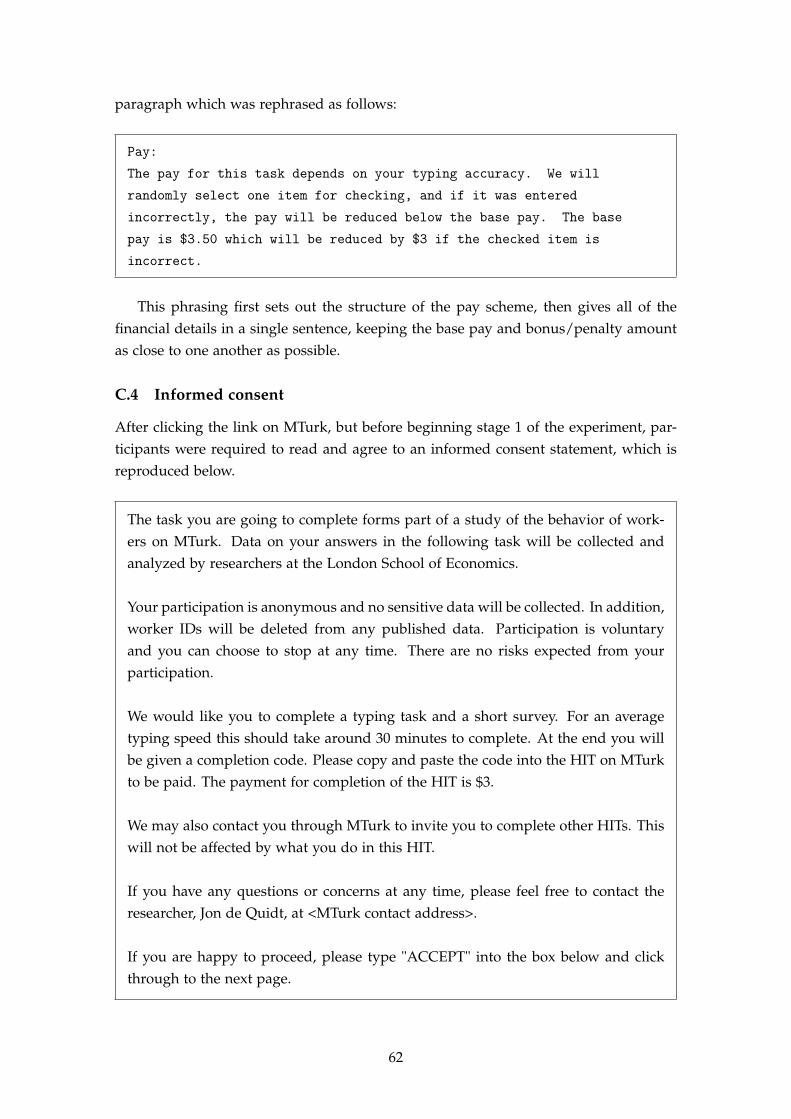
paragraph which was rephrased as follows:

Pay:

The pay for this task depends on your typing accuracy. We will

randomly select one item for checking, and if it was entered

incorrectly, the pay will be reduced below the base pay. The base

pay is $3.50 which will be reduced by $3 if the checked item is

incorrect.

This phrasing first sets out the structure of the pay scheme, then gives all of thefinancial details in a single sentence, keeping the base pay and bonus/penalty amountas close to one another as possible.

C.4 Informed consent

After clicking the link on MTurk, but before beginning stage 1 of the experiment, par-ticipants were required to read and agree to an informed consent statement, which isreproduced below.

The task you are going to complete forms part of a study of the behavior of work-ers on MTurk. Data on your answers in the following task will be collected andanalyzed by researchers at the London School of Economics.

Your participation is anonymous and no sensitive data will be collected. In addition,worker IDs will be deleted from any published data. Participation is voluntaryand you can choose to stop at any time. There are no risks expected from yourparticipation.

We would like you to complete a typing task and a short survey. For an averagetyping speed this should take around 30 minutes to complete. At the end you willbe given a completion code. Please copy and paste the code into the HIT on MTurkto be paid. The payment for completion of the HIT is $3.

We may also contact you through MTurk to invite you to complete other HITs. Thiswill not be affected by what you do in this HIT.

If you have any questions or concerns at any time, please feel free to contact theresearcher, Jon de Quidt, at <MTurk contact address>.

If you are happy to proceed, please type "ACCEPT" into the box below and clickthrough to the next page.

62

C.5 Lottery Questions

Figure C.1: Introduction and examples of lottery questions.

63