arX

iv:1

904.

0504

9v3

[cs

.CV

] 1

8 A

ug 2

019

Drop an Octave: Reducing Spatial Redundancy in

Convolutional Neural Networks with Octave Convolution

Yunpeng Chen†‡, Haoqi Fan†, Bing Xu†, Zhicheng Yan†, Yannis Kalantidis†,

Marcus Rohrbach†, Shuicheng Yan‡♭, Jiashi Feng‡

†Facebook AI, ‡National University of Singapore, ♭Yitu Technology

Abstract

In natural images, information is conveyed at different

frequencies where higher frequencies are usually encoded

with fine details and lower frequencies are usually encoded

with global structures. Similarly, the output feature maps of

a convolution layer can also be seen as a mixture of infor-

mation at different frequencies. In this work, we propose

to factorize the mixed feature maps by their frequencies,

and design a novel Octave Convolution (OctConv) opera-

tion1 to store and process feature maps that vary spatially

“slower” at a lower spatial resolution reducing both mem-

ory and computation cost. Unlike existing multi-scale meth-

ods, OctConv is formulated as a single, generic, plug-and-

play convolutional unit that can be used as a direct replace-

ment of (vanilla) convolutions without any adjustments in

the network architecture. It is also orthogonal and comple-

mentary to methods that suggest better topologies or reduce

channel-wise redundancy like group or depth-wise convolu-

tions. We experimentally show that by simply replacing con-

volutions with OctConv, we can consistently boost accuracy

for both image and video recognition tasks, while reduc-

ing memory and computational cost. An OctConv-equipped

ResNet-152 can achieve 82.9% top-1 classification accu-

racy on ImageNet with merely 22.2 GFLOPs.

1. Introduction

The efficiency of Convolutional Neural Networks

(CNNs) keeps increasing with recent efforts to reduce the

inherent redundancy in dense model parameters [15, 31, 42]

and in the channel dimension of feature maps [47, 18, 6, 9].

However, substantial redundancy also exists in the spatial

dimension of the feature maps produced by CNNs, where

each location stores its own feature descriptor indepen-

dently, while ignoring common information between adja-

cent locations that could be stored and processed together.

As shown in Figure 1(a), a natural image can be decom-

1https://github.com/facebookresearch/OctConv

(a) Separating the low and high spatial frequency signal [1, 10].

!"#$%&'()'*+,

-./0$%&'()'*+,

!"#$%&'()'*+,

-./0$%&'()'*+,

.*1"&234."*$'5+03*/'

.*1"&234."*$)6734'

(b)

!"#$%&'()'*+,

-./0$%&'()'*+,

!"#$%&'()'*+,

-./0$%&'()'*+,

.*1"&234."*$'5+03*/'

.*1"&234."*$)6734'

(c)

!"#$%&'()'*+,

-./0$%&'()'*+,

!"#$%&'()'*+,

-./0$%&'()'*+,

.*1"&234."*$'5+03*/'

.*1"&234."*$)6734'

(d)

Figure 1: (a) Motivation. The spatial frequency model for

vision [1, 10] shows that natural image can be decomposed

into a low and a high spatial frequency part. (b) The out-

put maps of a convolution layer can also be factorized and

grouped by their spatial frequency. (c) The proposed multi-

frequency feature representation stores the smoothly chang-

ing, low-frequency maps in a low-resolution tensor to re-

duce spatial redundancy. (d) The proposed Octave Convo-

lution operates directly on this representation. It updates the

information for each group and further enables information

exchange between groups.

posed into a low spatial frequency component that describes

the smoothly changing structure and a high spatial fre-

quency component that describes the rapidly changing fine

details [1, 10, 37, 39]. Similarly, we argue that the output

feature maps of a convolution layer can also be decomposed

into features of different spatial frequencies and propose a

novel multi-frequency feature representation which stores

high- and low-frequency feature maps into different groups

as shown in Figure 1(b). Thus, the spatial resolution of the

low-frequency group can be safely reduced by sharing in-

formation between neighboring locations to reduce spatial

redundancy as shown in Figure 1(c). To accommodate the

novel feature representation, we generalize the vanilla con-

volution, and propose Octave Convolution (OctConv) which

1

takes in feature maps containing tensors of two frequencies

one octave apart, and extracts information directly from the

low-frequency maps without the need of decoding it back

to the high-frequency as shown in Figure 1(d). As a re-

placement of vanilla convolution, OctConv consumes sub-

stantially less memory and computational resources. In ad-

dition, OctConv processes low-frequency information with

corresponding (low-frequency) convolutions and effectively

enlarges the receptive field in the original pixel space and

thus can improve recognition performance.

We design the OctConv in a generic way, making it

a plug-and-play replacement for the vanilla convolution.

Since OctConv mainly focuses on processing feature maps

at multiple spatial frequencies and reducing their spatial

redundancy, it is orthogonal and complementary to ex-

isting methods that focus on building better CNN topol-

ogy [22, 41, 35, 33, 29], reducing channel-wise redundancy

in convolutional feature maps [47, 9, 34, 32, 21] and re-

ducing redundancy in dense model parameters [42, 15, 31].

Moreover, different from methods that exploit multi-scale

information [4, 43, 12], OctConv can be easily deployed

as a plug-and-play unit to replace convolution, without

the need of changing network architectures or requiring

hyper-parameters tuning. Compared to the closely related

Multi-grid convolution [25], OctConv provides more in-

sights on reducing the spatial redundancy in CNNs based

on the frequency model and adopts more efficient inter-

frequency information exchange strategy with better perfor-

mance. We further integrate the OctConv into a wide vari-

ety of backbone architectures (including the ones featuring

group, depth-wise, and 3D convolutions) and demonstrate

universality of OctConv.

Our experiments demonstrate that by simply replacing

the vanilla convolution with OctConv, we can consistently

improve the performance of popular 2D CNN backbones

including ResNet [16, 17], ResNeXt [47], DenseNet [22],

MobileNet [18, 34] and SE-Net [19] on 2D image recog-

nition on ImageNet [11], as well as 3D CNN backbones

C2D [44] and I3D [44] on video action recognition on Ki-

netics [24, 3, 2]. The OctConv-equipped Oct-ResNet-152

can match or outperform state-of-the-art manually designed

networks [32, 19] at lower memory and computational cost.

Our contributions can be summarized as follows:

• We propose to factorize convolutional feature maps into

two groups at different spatial frequencies and process

them with different convolutions at their corresponding

frequency, one octave apart. As the resolution for low

frequency maps can be reduced, this saves both storage

and computation. This also helps each layer gain a larger

receptive field to capture more contextual information.

• We design a plug-and-play operation named OctConv to

replace the vanilla convolution for operating on the new

feature representation directly and reducing spatial re-

dundancy. Importantly, OctConv is fast in practice and

achieves a speedup close to the theoretical limit.

• We extensively study the properties of the proposed Oct-

Conv on a variety of backbone CNNs for image and video

tasks and achieve significant performance gain even com-

parable to the best AutoML networks.

2. Related Work

Improving the efficiency of CNNs. Ever since the pio-

neering work on AlexNet [26] and VGG [35], researchers

have made substantial efforts to improve the efficiency of

CNNs. ResNet [16, 17] and DenseNet [22] improve the

network topology by adding shortcut connections to early

layers. ResNeXt [47] and ShuffleNet [49] use sparsely con-

nected group convolutions to reduce redundancy in inter-

channel connectivity. Xception [9] and MobileNet [18, 34]

adopt depth-wise convolutions that further reduce the con-

nection density. Meanwhile, NAS [51], PNAS [29] and

AmoebaNet [33] propose to atomically find the best net-

work topology for a given task. Pruning methods, such

as DSD [15] and ThiNet [31], focus on reducing the re-

dundancy in the model parameters by eliminating the least

significant weight or connections in CNNs. Besides, Het-

Conv [36] propose to replace the vanilla convolution fil-

ters with heterogeneous convolution filters that are in dif-

ferent sizes. However, all of these methods ignore the re-

dundancy on the spatial dimension of feature maps, which

is addressed by the proposed OctConv, making OctConv

orthogonal and complementary to these previous methods.

Noticeably, OctConv does not change the connectivity be-

tween feature maps, making it also different from inception-

alike multi-path designs [41, 40, 47].

Multi-scale Representation Learning. Prior to the suc-

cess of deep learning, multi-scale representation has long

been applied for local feature extraction, such as the SIFT

features [30]. In the deep learning era, multi-scale repre-

sentation also plays a important role due to its strong ro-

bustness and generalization ability. FPN [27] and PSP [50]

merge convolutional features from different depths at the

end of the networks for object detection and segmenta-

tion tasks. MSDNet [20] and HR-Nets [38], proposed

carefully designed network architectures that contain mul-

tiple branches where each branch has it own spatial resolu-

tion. The bL-Net [4] and ELASTIC-Net [43] adopt similar

idea, but are designed as a replacement of residual block

for ResNet [16, 17] and thus are more flexible and eas-

ier to use. But extra expertise and hyper-parameter tun-

ing are still required when adopt them to architectures be-

yond ResNet, such as MobileNetV1 [18], DenseNet [22].

Multi-grid CNNs [25] propose a multi-grid pyramid feature

representation and define the MG-Conv operator as a re-

placement of convolution operator, which is conceptually

similar to our method but is motivated for exploiting multi-

scale features. Compared with MG-Conv, OctConv adopts

more efficient design to exchange inter-frequency informa-

tion with higher performance as can be found in Sec. 3.3 and

Sec. 4.3. For video models, the recently proposed Slow-

Fast Networks [12] introduce multi-scale pathways on the

temporal dimension. As we show in Section 4.4, this is

complementary to OctConv which operates on the spatial

dimensions.

In a nutshell, OctConv focuses on reducing the spatial re-

dundancy in CNNs and is designed to replace vanilla convo-

lution operations without needing to adjust backbone CNN

architecture. We extensively compare OctConv to closely

related methods in the sections of method and experiment

and show that OctConv CNNs give top results on a number

of challenging benchmarks.

3. Method

In this section, we first introduce the octave feature rep-

resentation and then describe Octave Convolution, which

operates directly on it. We also discuss implementation de-

tails and show how to integrate OctConv into group and

depth-wise convolution architectures.

3.1. Octave Feature Representation

For the vanilla convolution, all input and output feature

maps have the same spatial resolution, which may not be

necessary since some of the feature maps may represent

low-frequency information which is spatially redundant and

can be further compressed as illustrated in Figure 1.

To reduce the spatial redundancy, we introduce the oc-

tave feature representation that explicitly factorizes the fea-

ture map tensors into groups corresponding to low and high

frequencies. The scale-space theory [28] provides us with

a principled way of creating scale-spaces of spatial resolu-

tions, and defines an octave as a division of the spatial di-

mensions by a power of 2 (we only explore 21 in this work).

We follow this fashion and reduce the spatial resolution of

the low-frequency feature maps by an octave.

Formally, let X ∈ Rc×h×w denote the input feature ten-

sor of a convolutional layer, where h and w denote the spa-

tial dimensions and c the number of feature maps or chan-

nels. We explicitly factorizeX along the channel dimension

into X = {XH , XL}, where the high-frequency feature

maps XH ∈ R(1−α)c×h×w capture fine details and the low-

frequency maps XL ∈ Rαc×h

2×w

2 vary slower in the spatial

dimensions (w.r.t. the image locations). Here α ∈ [0, 1]denotes the ratio of channels allocated to the low-frequency

part and the low-frequency feature maps are defined an oc-

tave lower than the high frequency ones, i.e. at half of the

spatial resolution as shown in Figure 1(c).

In the next subsection, we introduce a convolution op-

erator that operates directly on this multi-frequency feature

representation and name it Octave Convolution (OctConv).

3.2. Octave Convolution

The octave feature representation presented in Sec-

tion 3.1 reduces the spatial redundancy and is more compact

than the original representation. However, the vanilla con-

volution cannot directly operate on such a representation,

due to differences in spatial resolution in the input features.

A naive way of circumventing this is to up-sample the low-

frequency part XL to the original spatial resolution, con-

catenate it with XH and then convolve, which would lead

to extra costs in computation and memory and diminish all

the savings from the compression. In order to fully exploit

our compact multi-frequency feature representation, we in-

troduce Octave Convolution, which can directly operate on

factorized tensors X = {XH , XL} without requiring any

extra computational or memory overhead.

Vanilla Convolution. Let W ∈ Rc×k×k denote a k × k

convolution kernel and X,Y ∈ Rc×h×w denote the input

and output tensors, respectively. Each feature map in Yp,q ∈R

c can be computed by

Yp,q =∑

i,j∈Nk

Wi+ k−1

2,j+ k−1

2

⊤Xp+i,q+j , (1)

where (p, q) denotes the location coordinate and Nk ={(i, j) : i = {−k−1

2 , . . . , k−12 }, j = {−k−1

2 , . . . , k−12 }}

defines a local neighborhood. For simplicity, in all equa-

tions we omit the padding, we assume k is an odd number

and that the input and output data have the same dimension-

ality, i.e. cin = cout = c.

Octave Convolution. The goal of our design is to effec-

tively process the low and high frequency in their corre-

sponding frequency tensor but also enable efficient inter-

frequency communication. Let X,Y be the factorized in-

put and output tensors. Then the high- and low-frequency

feature maps of the output Y = {Y H , Y L} will be given

by Y H = Y H→H + Y L→H and Y L = Y L→L + Y H→L,

respectively, where Y A→B denotes the convolutional up-

date from feature map group A to group B. Specifi-

cally, Y H→H , Y L→L denote intra-frequency update, while

Y H→L, Y L→H denote inter-frequency communication.

To compute these terms, we split the convolutional ker-

nel W into two components W = [WH ,WL] responsi-

ble for convolving with XH and XL respectively. Each

component can be further divided into intra- and inter-

frequency part: WH = [WH→H ,WL→H ] and WL =[WL→L,WH→L] with the parameter tensor shape shown

in Figure 2(b). Specifically for high-frequency feature map,

we compute it at location (p, q) by using a regular con-

volution for the intra-frequency update, and for the inter-

frequency communication we can fold the up-sampling over

the feature tensor XL into the convolution, removing the

need of explicitly computing and storing the up-sampled

(a) Detailed design of the Octave Convolution. Green arrows corre-

spond to information updates while red arrows facilitate information

exchange between the two frequencies.

(b) The Octave Convolution kernel. The k × k Octave

Convolution kernel W ∈ Rcin×cout×k×k is equivalent

to the vanilla convolution kernel in the sense that the

two have the exact same number of parameters.

Figure 2: Octave Convolution. We set αin = αout = α throughout the network, apart from the first and last OctConv of the

network where αin = 0, αout = α and αin = α, αout = 0, respectively.

feature maps as follows:

Y Hp,q =Y H→H

p,q + Y L→Hp,q

=∑

i,j∈Nk

WH→H

i+ k−1

2,j+ k−1

2

⊤XH

p+i,q+j

+∑

i,j∈Nk

WL→H

i+ k−1

2,j+ k−1

2

⊤XL

(⌊ p

2⌋+i),(⌊ q

2⌋+j),

(2)

where ⌊·⌋ denotes the floor operation. Similarly, for the

low-frequency feature map, we compute the intra-frequency

update using a regular convolution. Note that, as the map is

in one octave lower, the convolution is also low-frequency

w.r.t. the high-frequency coordinate space. For the inter-

frequency communication we can again fold the down-

sampling of the feature tensor XH into the convolution as

follows:

Y Lp,q =Y L→L

p,q + Y H→Lp,q

=∑

i,j∈Nk

WL→L

i+ k−1

2,j+ k−1

2

⊤XL

p+i,q+j

+∑

i,j∈Nk

WH→L

i+ k−1

2,j+ k−1

2

⊤XH

(2∗p+0.5+i),(2∗q+0.5+j),

(3)

where multiplying a factor 2 to the locations (p, q) performs

down-sampling, and further shifting the location by half

step is to ensure the down-sampled maps well aligned with

the input. However, since the index of XH can only be an

integer, we could either round the index to (2∗p+i, 2∗q+j)or approximate the value at (2 ∗ p+0.5+ i, 2 ∗ q+0.5+ j)by averaging all 4 adjacent locations. The first one is also

known as strided convolution and the second one as average

pooling. As we discuss in Section 3.3 and Fig. 5, strided

convolution leads to misalignment; we therefore use aver-

age pooling to approximate this value for the rest of the pa-

per.

An interesting and useful property of the Octave Con-

volution is the larger receptive field for the low-frequency

feature maps. Convolving the low-frequency part XL with

k × k convolution kernels, results in an effective enlarge-

ment of the receptive field by a factor of 2 compared to

vanilla convolutions. This further helps each OctConv layer

capture more contextual information from distant locations

and can potentially improve recognition performance.

3.3. Implementation Details

As discussed in the previous subsection, the index {(2 ∗p + 0.5 + i), (2 ∗ q + 0.5 + j)} has to be an integer for

Eq. 3. Instead of rounding it to {(2 ∗ p + i), (2 ∗ q + j)},

i.e. conduct convolution with stride 2 for down-sampling,

we adopt average pooling to get more accurate approxima-

tion. This helps alleviate misalignments that appear when

aggregating information from different scales, as shown in

Appendix A. and Appendix C.. We can now rewrite the

output Y = {Y H , Y L} of the Octave Convolution using

average pooling for down-sampling as:

Y H =f(XH ;WH→H) + upsample(f(XL;WL→H), 2)

Y L =f(XL;WL→L) + f(pool(XH , 2);WH→L)),(4)

where f(X ;W ) denotes a convolution with parameters W ,

pool(X, k) is an average pooling operation with kernel size

k × k and stride k. upsample(X, k) is an up-sampling op-

eration by a factor of k via nearest interpolation.

The details of the OctConv operator implementation are

shown in Figure 2. It consists of four computation paths

that correspond to the four terms in Eq. (4): two green paths

correspond to information updating for the high- and low-

frequency feature maps, and two red paths facilitate infor-

mation exchange between the two octaves.

Group and Depth-wise convolutions. The Octave Convo-

lution can also be adopted to other popular variants of the

vanilla convolution such as group [47] or depth-wise [18]

convolutions. For the group convolution case, we simply

set all four convolution operations that appear inside the

design of the OctConv to group convolutions. Similarly,

for the depth-wise convolution case, the convolution opera-

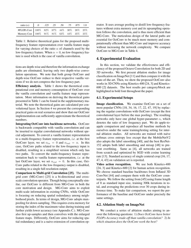
ratio (α) .0 .125 .25 .50 .75 .875 1.0

#FLOPs Cost 100% 82% 67% 44% 30% 26% 25%

Memory Cost 100% 91% 81% 63% 44% 35% 25%

Table 1: Relative theoretical gains for the proposed multi-

frequency feature representation over vanilla feature maps

for varying choices of the ratio α of channels used by the

low-frequency feature. When α = 0, no low-frequency fea-

ture is used which is the case of vanilla convolution.

tions are depth-wise and therefore the information exchange

paths are eliminated, leaving only two depth-wise convo-

lution operations. We note that both group OctConv and

depth-wise OctConv reduce to their respective vanilla ver-

sions if we do not compress the low-frequency part.

Efficiency analysis. Table 1 shows the theoretical com-

putational cost and memory consumption of OctConv over

the vanilla convolution and vanilla feature map represen-

tation. More information on deriving the theoretical gains

presented in Table 1 can be found in the supplementary ma-

terial. We note the theoretical gains are calculated per con-

volutional layer. In Section 4 we present the corresponding

practical gains on real scenarios and show that our OctConv

implementation can sufficiently approximate the theoretical

numbers.

Integrating OctConv into backbone networks. OctConv

is backwards compatible with vanilla convolution and can

be inserted to regular convolutional networks without spe-

cial adjustment. To convert a vanilla feature representation

to a multi-frequency feature representation, i.e. at the first

OctConv layer, we set αin = 0 and αout = α. In this

case, OctConv paths related to the low-frequency input is

disabled, resulting in a simplified version which only has

two paths. To convert the multi-frequency feature repre-

sentation back to vanilla feature representation, i.e. at the

last OctConv layer, we set αout = 0. In this case, Oct-

Conv paths related to the low-frequency output is disabled,

resulting in a single full resolution output.

Comparison to Multi-grid Convolution [25]. The multi-

grid conv (MG-Conv) [25] is a bi-directional and cross-

scale convolution operator. Though being conceptually sim-

ilar, our OctConv is different from MG-Conv in both the

core motivation and design. MG-Conv aims to exploit

multi-scale information in existing CNNs, while OctConv

is focusing on reducing spatial redundancy among neigh-

borhood pixels. In terms of design, MG-Conv adopts max-

pooling for down-sampling. This requires extra memory for

storing the index of the maximum value during training and

further yields lower accuracy (see Appendix C.). MG-Conv

also first up-samples and then convolves with the enlarged

feature maps. Differently, OctConv aims for reducing spa-

tial redundancy and is a naive extension of convolution op-

erator. It uses average pooling to distill low-frequency fea-

tures without extra memory cost and its upsampling opera-

tion follows the convolution, and is thus more efficient than

MG-Conv. The meticulous design of the lateral paths are

essential for OctConv to be much more memory and com-

putationally efficient than MG-Conv and improve accuracy

without increasing the network complexity. We compare

OctConv to MG-Conv in Table 4.

4. Experimental Evaluation

In this section, we validate the effectiveness and effi-

ciency of the proposed Octave Convolution for both 2D and

3D networks. We first present ablation studies for image

classification on ImageNet [11] and then compare it with the

state-of-the-art. Then, we show the proposed OctConv also

works in 3D CNNs using Kinetics-400 [24, 3] and Kinetics-

600 [2] datasets. The best results per category/block are

highlighted in bold font throughout the paper.

4.1. Experimental Setups

Image classification. We examine OctConv on a set of

most popular CNNs [18, 34, 16, 17, 22, 47, 19] by replac-

ing the regular convolutions with OctConv (except the first

convolutional layer before the max pooling). The resulting

networks only have one global hyper-parameter α, which

denotes the ratio of low frequency part. We do apple-to-

apple comparison and reproduce all baseline methods by

ourselves under the same training/testing setting for inter-

nal ablation studies. All networks are trained with naıve

softmax cross entropy loss except that the MobileNetV2

also adopts the label smoothing [40], and the best ResNet-

152 adopts both label smoothing and mixup [48] to pre-

vent overfitting. Same as [4], all networks are trained

from scratch and optimized by SGD with cosine learning

rate [13]. Standard accuracy of single centeral crop [16, 17,

47, 4, 43] on validation set is reported.

Video action recognition. We use both Kinetics-400

[24, 3] and Kinetics-600 [2] for human action recognition.

We choose standard baseline backbones from Inflated 3D

ConvNet [44] and compare them with the OctConv coun-

terparts. We follow the setting from [45] using frame length

of 8 as standard input size, training 300k iterations in to-

tal, and averaging the predictions over 30 crops during in-

ference time. To make fair comparison, we report the per-

formance of the baseline and OctConv under precisely the

same settings.

4.2. Ablation Study on ImageNet

We conduct a series of ablation studies aiming to an-

swer the following questions: 1) Does OctConv have better

FLOPs-Accuracy trade-off than vanilla convolution? 2) In

which situation does the OctConv work the best?

1 1.25 1.5 2 2.5 3 4 5 6 7 8 9 10 12 14 16

74

76

78

80

FLOPs (×109)

Top-1

Acc

ura

cy(%

)

0.06250.125

0.250.125

0.25

0.50

0.75

0.25

0.50

0.75

0.125

0.25

0.50

0.75

0.1250.25

0.5

0.25

0.5

0.1250.25

0.50

0.1250.25

0.50

0.75

ResNet-26

ResNet-50

SE-ResNet-50

ResNeXt-50 ResNet-101

ResNeXt-101

DenseNet-121

ResNet-200

Figure 3: Ablation study results on ImageNet. OctConv-

equipped models are more efficient and accurate than base-

line models. Markers in black in each line denote the cor-

responding baseline models without OctConv. The colored

numbers are the ratio α. Numbers in X axis denote FLOPs

in logarithmic scale.

Results on ResNet-50. We begin with using the popu-

lar ResNet-50 [17] as the baseline CNN and replacing the

regular convolution with our proposed OctConv to exam-

ine the flops-accuracy trade-off. In particular, we vary the

global ratio α ∈ {0.125, 0.25, 0.5, 0.75} to compare the im-

age classification accuracy versus computational cost (i.e.

FLOPs) [16, 17, 47, 7] with the baseline. The results are

shown in Figure 3 in pink.

We make following observations. 1) The flops-accuracy

trade-off curve is a concave curve, where the accuracy first

rises up and then slowly goes down. 2) We can see two

sweet spots: The first at α = 0.5, where the network gets

similar or better results even when the FLOPs are reduced

by about half; the second at α = 0.125, where the network

reaches its best accuracy, 1.2% higher than baseline (black

circle). We attribute the increase in accuracy to OctConv’s

effective design of multi-frequency processing and the cor-

responding enlarged receptive field which provides more

contextual information to the network. While reaching the

accuracy peak at 0.125, the accuracy does not suddenly drop

but decreases slowly for higher ratios α, indicating reduc-

ing the resolution of the low frequency part does not lead

to significant information loss. Interestingly, 75% of the

feature maps can be compressed to half the resolution with

only 0.3% accuracy drop, which demonstrates effectiveness

of grouping and compressing the smoothly changed feature

maps for reducing the spatial redundancy in CNNs. In Ta-

ble 2 we demonstrate the theoretical FLOPs saving of Oct-

Conv is also reflected in the actual CPU inference time in

practice. For ResNet-50, we are close to obtaining theo-

retical FLOPs speed up. These results indicate OctConv is

able to deliver important practical benefits, rather than only

saving FLOPs in theory.

ratio (α) Top-1 (%) #FLOPs (G) Inference Time (ms) Backend

N/A 77.0 4.1 119 MKLDNN

N/A 77.0 4.1 115 TVM

.125 78.2 3.6 116 TVM

.25 78.0 3.1 99 TVM

.5 77.4 2.4 74 TVM

.75 76.7 1.9 61 TVM

Table 2: Results of ResNet-50. Inference time is measured

on Intel Skylake CPU at 2.0 GHz (single thread). We report

Intel(R) Math Kernel Library for Deep Neural Networks

v0.18.1 (MKLDNN) [23] inference time for vanila ResNet-

50. Because vanilla ResNet-50 is well optimized by Intel,

we also show MKLDNN results as additional performance

baseline. OctConv networks are compiled by TVM [5] v0.5.

Oct-High-Frequency Group Oct-Low-Frequency GroupBaseline Low→ High Freq

Energy

Figure 4: Frequency analysis for activation maps in differ-

ent groups. ‘Baseline‘ refers to vanilla ResNet. 10k activa-

tion maps are sampled from ResNet-101(Res3).

Results on more CNNs. To further examine if the pro-

posed OctConv works for other networks with different

depth/wide/topology, we select the currently most popu-

lar networks as baselines and repeat the same ablation

study. These networks are ResNet-(26;50;101;200) [17],

ResNeXt-(50,32×4d;101,32×4d) [47], DenseNet-121 [22]

and SE-ResNet-50 [19]. The ResNeXt is chosen for as-

sessing the OctConv on group convolution, while the SE-

Net [19] is used to check if the gain of SE block found

on vanilla convolution based networks can also be seen

on OctConv. As shown in Figure 3, OctConv equipped

networks for different architecture behave similarly to the

Oct-ResNet-50, where the FLOPs-Accuracy trade-off is in

a concave curve and the performance peak also appears at

ratio α = 0.125 or α = 0.25. The consistent performance

gain on a variety of backbone CNNs confirms that OctConv

is a good replacement of vanilla convolution.

Frequency Analysis. Figure 4 shows the frequency anal-

ysis results. We conducted the Fourier transform for each

group of feature maps and visualized the averaged results.

From the energy map, the low frequency group does not

contain high frequency signal, while the high frequency

group contains both low and high frequency signals. This

confirms that low-frequency group indeed captures low-

frequency information as expected. Note that OctConv

gives the high frequency group the flexibly to store both

low and high frequency signals for better learning capacity.

Summary. 1) OctConv can help CNNs improve the ac-

curacy while decreasing the FLOPs, deviating from other

methods that reduce the FLOPs with a cost of lower ac-

curacy. 2) At test time, the gain of OctConv over baseline

Method ratio (α) #Params (M) #FLOPs (M) CPU (ms) Top-1 (%)

CondenseNet (G = C = 8) [21] - 2.9 274 - 71.0

1.5 ShuffleNet (v1) [49] - 3.4 292 - 71.5

1.5 ShuffleNet (v2) [32] - 3.5 299 - 72.6

0.75 MobileNet (v1) [18] - 2.6 325 13.4 70.3∗

0.75 Oct-MobileNet (v1) (ours) .375 2.6 213 11.9 70.5

1.0 Oct-MobileNet (v1) (ours) .5 4.2 321 18.4 72.5

1.0 MobileNet (v2) [34] - 3.5 300 24.5 72.0

1.0 Oct-MobileNet (v2) (ours) .375 3.5 256 17.1 72.0

1.125 Oct-MobileNet (v2) (ours) .5 4.2 295 26.3 73.0

Table 3: ImageNet classification results for Small models.∗ indicates it is better than original reproduced by MXNet

GluonCV v0.4 [14]. The inference speed is tested using

TVM on Intel Skylake processor (2.0GHz, single thread)2.

Method ratio (α) Depth #Params (M) #FLOPs (G) Top-1 (%)

R-MG-34 [25] - 34 32.9 5.8 75.5

Oct-ResNet-26 (ours) .25 26 16.0 1.9 76.1

Oct-ResNet-50 (ours) .5 50 25.6 2.4 77.4

ResNet-50 + GloRe [8] (+3 blocks Res4) - 50 30.5 5.2 78.4

Oct-ResNet-50 (ours) + GloRe [8] (+3 blocks Res4) .5 50 30.5 3.1 78.8

ResNeXt-50 + Elastic [43] - 50 25.2 4.2 78.4

Oct-ResNeXt-50 (32×4d) (ours) .25 50 25.0 3.2 78.8

ResNeXt-101 + Elastic [43] - 101 44.3 7.9 79.2

Oct-ResNeXt-101 (32×4d) (ours) .25 101 44.2 5.7 79.6

bL-ResNet-50‡ (α = 4, β = 4) [4] - 50 (+3) 26.2 2.5 76.9

Oct-ResNet-50‡ (ours) .5 50 (+3) 25.6 2.5 77.8

Oct-ResNet-50 (ours) .5 50 25.6 2.4 77.4

bL-ResNeXt-50‡ (32×4d) [4] - 50 (+3) 26.2 3.0 78.4

Oct-ResNeXt-50‡ (32×4d) (ours) .5 50 (+3) 25.1 2.7 78.6

Oct-ResNeXt-50 (32×4d) (ours) .5 50 25.0 2.4 78.4

bL-ResNeXt-101‡ § (32×4d) [4] - 101 (+1) 43.4 4.1 78.9

Oct-ResNeXt-101‡ § (32×4d) (ours) .5 101 (+1) 40.1 4.2 79.4

Oct-ResNeXt-101‡ (32×4d) (ours) .5 101 (+1) 44.2 4.2 79.1

Oct-ResNeXt-101 (32×4d) (ours) .5 101 44.2 4.0 78.9

Table 4: ImageNet Classification results for Middle sized

models. ‡ refers to method that replaces “Max Pooling” by

extra convolution layer(s) [4]. § refers to method that uses

balanced residual block distribution [4].

models increases as the test image resolution grows because

OctConv can detect large objects better due to its larger re-

ceptive field, see Appendix C. 3) Both the information ex-

changing paths are important, since removing any of them

can lead to accuracy drop, see Appendix C. 4) Shallow net-

works, e.g. ResNet-26, have a rather limited receptive field,

and can especially benefit from OctConv, which greatly en-

larges their receptive field.

4.3. Comparing with SOTAs on ImageNet

Small models. We adopt the most popular light weight

networks as baselines and examine if OctConv works well

on these compact networks with depth-wise convolution. In

particular, we use the “0.75 MobileNet (v1)” [18] and “1.0

MobileNet (v2)” [34] as baseline and replace the regular

convolution with our proposed OctConv. The results are

shown in Table 3. We find that OctConv can reduce the

FLOPs of MobileNetV1 by 34%, and provide better accu-

racy and faster speed in practice; it is able to reduce the

FLOPs of MobileNetV2 by 15%, achieving the same ac-

curacy with faster speed. When the computation budget is

fixed, one can adopt wider models to increase the learning

capacity because OctConv can compensate the extra com-

putation cost. In particular, our OctConv equipped networks

achieve 2% improvement on MobileNetV1 under the same

FLOPs and 1% improvement on MobileNetV2.

Medium models. In the above experiment, we have com-

pared and shown that OctConv is complementary with a

set of state-of-the-art CNNs [16, 17, 47, 22, 18, 34, 19].

In this part, we compare OctConv with MG-Conv [25],

GloRe [8], Elastic [43] and bL-Net [4] which share a simi-

lar idea as our method. Seven groups of results are shown

in Table 4. In group 1, our Oct-ResNet-26 shows 0.6% bet-

ter accuracy than R-MG-34 while costing only one third

of FLOPs and half of #Params. Also, our Oct-ResNet-

50, which costs less than half of FLOPS, achieves 1.9%higher accuracy than R-MG-34. In group 2, adding our

OctConv to GloRe network reduces the FLOPs with bet-

ter accuracy. In group 3, our Oct-ResNeXt-50 achieves

better accuracy than the Elastic [43] based method (78.8%

v.s. 78.4%) while reducing the computational cost by 31%.

In group 4, the Oct-ResNeXt-101 also achieves higher ac-

curacy than the Elastic based method (79.6% v.s. 79.2%)

while costing 38% less computation. When compared to

the bL-Net [4], OctConv equipped methods achieve better

FLOPs-Accuracy trade-off without bells and tricks. When

adopting the tricks used in the baseline bL-Net [4], our Oct-

ResNet-50 achieves 0.9% higher accuracy than bL-ResNet-

50 under the same computational budget (group 5), and Oct-

ResNeXt-50 (group 6) and Oct-ResNeXt-101 (group 7) get

better accuracy under comparable or even lower compu-

tational budget. This is because MG-Conv [25], Elastic-

Net [43] and bL-Net [4] are designed following the prin-

ciple of introducing multi-scale features without consider-

ing reducing the spatial redundancy. In contrast, OctConv

is born for solving the high spatial redundancy problem in

CNNs, uses more efficient strategies to store and process the

information throughout the network, and can thus achieve

better efficiency and performance.

Large models. Table 5 shows the results of OctConv in

large models. Here, we choose the ResNet-152 as the back-

bone CNN, replacing the first 7 × 7 convolution by three

3 × 3 convolution layers and removing the max pooling by

a lightweight residual block [4]. We report results for Oct-

ResNet-152 with and without the SE-block [19]. As can

be seen, our Oct-ResNet-152 achieves accuracy compara-

ble to the best manually designed networks with less FLOPs

(10.9G v.s. 12.7G). Since our model does not use group or

depth-wise convolutions, it also requires significantly less

GPU memory, and runs faster in practice compared to the

SE-ShuffleNet v2-164 and AmoebaNet-A (N=6, F=190)

which have low FLOPs in theory but run slow in practice

2For small models, we should notice according to arithmetic intensity

[46], real execution time is not only bounded by FLOPS.

Method #Params (M)Training Testing (224× 224) Testing (320× 320 / 331× 331)

Input Size Memory Cost (MB) Speed (im/s) #FLOPs (G) Top-1 (%) Top-5 (%) #FLOPs (G) Top-1 (%) Top-5 (%)

NASNet-A (N=6, F=168) [51] 3 88.9

331× 331/ 320× 320

> 32, 480 43 ‡ - - - 23.8 82.7 96.2

AmoebaNet-A (N=6, F=190) [33] 3 86.7 > 32, 480 47 ‡ - - - 23.1 82.8 96.1

PNASNet-5 (N=4, F=216) [29] 3 86.1 > 32, 480 38 ‡ - - - 25.0 82.9 96.2

Squeeze-Excite-Net [19] 115.1 > 32, 480 43 † - - - 42.3 83.1 96.4

AmoebaNet-A (N=6, F=448) [33] 3 469 > 32, 480 15 § - - - 104 83.9 96.6

Dual-Path-Net-131 [7] 79.5

224× 224

31,844 83 16.0 80.1 94.9 32.0 81.5 95.8

SE-ShuffleNet v2-164 [32] 69.9 > 32, 480 70 † 12.7 81.4 - - - -

Squeeze-Excite-Net [19] 115.1 28,696 78 21 81.3 95.5 42.3 82.7 96.2

Oct-ResNet-152, α = 0.125 (ours) 60.2 15,566 162 10.9 81.4 95.4 22.2 82.3 96.0

Oct-ResNet-152 + SE3, α = 0.125 (ours) 66.8 21,885 95 10.9 81.6 95.7 22.2 82.9 96.3

Table 5: ImageNet Classification results for Large models. The names of OctConv-equiped models are in bold font and

performance numbers for related works are copied from the corresponding papers. Networks are evaluated using CuDNN

v10.04in flop16 on a single Nvidia Titan V100 (32GB) for their training memory cost and speed. Works that employ neural

architecture search are denoted by (3). We set batch size to 128 in most cases, but had to adjust it to 64 (noted by †), 32

(noted by ‡) or 8 (noted by §) for networks that are too large to fit into GPU memory.

due to the use of group and depth-wise convolutions. Our

proposed method is also complementary to Squeeze-and-

excitation [19], where the accuracy can be further boosted

when the SE-Block is added (last row).

4.4. Experiments of Video Recognition on Kinetics

In this subsection, we evaluate the effectiveness of Oct-

Conv for action recognition in videos and demonstrate that

our spatial OctConv is sufficiently generic to be integrated

into 3D convolution to decrease #FLOPs and increase ac-

curacy at the same time. As shown in Table 6, OctConv

consistently decreases FLOPs and meanwhile improves the

accuracy when added to C2D and I3D [44, 45], and is also

complementary to the Non-local [44]. This is observed

for models pre-trained on ImageNet [11] as well as mod-

els trained from scratch on Kinetics. The higher accuracy,

lower FLOPs and the ability of being complimentary to ex-

isting metods, e.g. Non-local method, confirm the effective-

ness of the proposed OctConv method. Performance further

increases when combining OctConv with the SlowFast Net-

works [12]. Specifically, we apply OctConv on the spatial

dimensions and SlowFast on the temporal dimension.

5. Conclusion

In this work, we address the problem of reducing spa-

tial redundancy that widely exists in vanilla CNN models,

and propose a novel Octave Convolution operation to store

and process low- and high-frequency features separately to

improve the model efficiency. Octave Convolution is suffi-

3The auto-tune is set to off when evaluating the memory cost for more

accurate result, and is set to on when measuring speed for fastest speed.4An extra BatchNorm is added at the beginning of each residual func-

tion, otherwise the gradient will easily diverged due to the newly added

SE module. This costs more memory and slows down the speed but can

provide higher accuracy.5Note that [12] reports 36.1 GFLOPs at a spatial size of 2562, while

we report (training) GFLOPs at 2242 for all methods.

Method ImageNet Pretrain #FLOPs (G) Top-1 (%)

(a) Kinetics-400 [3]

I3D 28.1 72.6

Oct-I3D, α=0.1, (ours) 25.6 73.6 (+1.0)

Oct-I3D, α=0.2, (ours) 22.1 73.1 (+0.5)

Oct-I3D, α=0.5, (ours) 15.3 72.1 (-0.5)

C2D � 19.3 71.9

Oct-C2D, α=0.1, (ours) � 17.4 73.8 (+1.9)

I3D � 28.1 73.3

Oct-I3D, α=0.1, (ours) � 25.6 74.6 (+1.3)

I3D + Non-local � 33.3 74.7

Oct-I3D + Non-local, α=0.1, (ours) � 28.9 75.7 (+1.0)

SlowFast-R50 [12] 27.6 5 75.6

Oct-SlowFast-R50, α=0.1, (ours) 24.5 76.2 (+0.6)

Oct-SlowFast-R50, α=0.2, (ours) 22.9 75.8 (+0.2)

(b) Kinetics-600 [2]

I3D � 28.1 74.3

Oct-I3D, α=0.1, (ours) � 25.6 76.0 (+1.7)

Table 6: Action Recognition in videos, ablation study, all

models with ResNet50 [16].

ciently generic to replace the regular convolution operation

in-place, and can be used in most 2D and 3D CNNs without

model architecture adjustment. Beyond saving a substan-

tial amount of computation and memory, Octave Convolu-

tion can also improve the recognition performance by effec-

tive communication between the low- and high-frequency

and by enlarging the receptive field size which contributes

to capturing more global information. Our extensive ex-

periments on image classification and video action recog-

nition confirm the superiority of our method for striking a

much better trade-off between recognition performance and

model efficiency, not only in FLOPs, but also in practice.

Acknowledgement. We would like to thank Min Lin and

Xin Zhao for helpful discussions of the code development.

References

[1] Fergus W Campbell and JG Robson. Application of fourier

analysis to the visibility of gratings. The Journal of physiol-

ogy, 197(3):551–566, 1968.

[2] Joao Carreira, Eric Noland, Andras Banki-Horvath, Chloe

Hillier, and Andrew Zisserman. A short note about kinetics-

600. arXiv preprint arXiv:1808.01340, 2018.

[3] Joao Carreira and Andrew Zisserman. Quo vadis, action

recognition? a new model and the kinetics dataset. In pro-

ceedings of the IEEE Conference on Computer Vision and

Pattern Recognition, pages 6299–6308, 2017.

[4] Chun-Fu Chen, Quanfu Fan, Neil Mallinar, Tom Sercu, and

Rogerio Feris. Big-little net: An efficient multi-scale feature

representation for visual and speech recognition. Proceed-

ings of the Seventh International Conference on Learning

Representations, 2019.

[5] Tianqi Chen, Thierry Moreau, Ziheng Jiang, Lianmin Zheng,

Eddie Yan, Haichen Shen, Meghan Cowan, Leyuan Wang,

Yuwei Hu, Luis Ceze, et al. {TVM}: An automated

end-to-end optimizing compiler for deep learning. In 13th

{USENIX} Symposium on Operating Systems Design and

Implementation ({OSDI} 18), pages 578–594, 2018.

[6] Yunpeng Chen, Yannis Kalantidis, Jianshu Li, Shuicheng

Yan, and Jiashi Feng. Multi-fiber networks for video recog-

nition. In Proceedings of the European Conference on Com-

puter Vision (ECCV), pages 352–367, 2018.

[7] Yunpeng Chen, Jianan Li, Huaxin Xiao, Xiaojie Jin,

Shuicheng Yan, and Jiashi Feng. Dual path networks. In

Advances in Neural Information Processing Systems, pages

4467–4475, 2017.

[8] Yunpeng Chen, Marcus Rohrbach, Zhicheng Yan, Shuicheng

Yan, Jiashi Feng, and Yannis Kalantidis. Graph-based global

reasoning networks. In Proceedings of the IEEE Conference

on Computer Vision and Pattern Recognition, 2019.

[9] Francois Chollet. Xception: Deep learning with depthwise

separable convolutions. In Proceedings of the IEEE con-

ference on computer vision and pattern recognition, pages

1251–1258, 2017.

[10] Russell L. De Valois and Karen K. De Valois. Spatial vision.

Oxford psychology series, No. 14., 1988.

[11] Jia Deng, Wei Dong, Richard Socher, Li-Jia Li, Kai Li,

and Li Fei-Fei. Imagenet: A large-scale hierarchical image

database. In 2009 IEEE conference on computer vision and

pattern recognition, pages 248–255. Ieee, 2009.

[12] Christoph Feichtenhofer, Haoqi Fan, Jitendra Malik, and

Kaiming He. Slowfast networks for video recognition.

ICCV, 2019.

[13] Priya Goyal, Piotr Dollar, Ross Girshick, Pieter Noord-

huis, Lukasz Wesolowski, Aapo Kyrola, Andrew Tulloch,

Yangqing Jia, and Kaiming He. Accurate, large mini-

batch sgd: Training imagenet in 1 hour. arXiv preprint

arXiv:1706.02677, 2017.

[14] Jian Guo, He He, Tong He, Leonard Lausen, Mu Li, Haibin

Lin, Xingjian Shi, Chenguang Wang, Junyuan Xie, Sheng

Zha, Aston Zhang, Hang Zhang, Zhi Zhang, Zhongyue

Zhang, and Shuai Zheng. Gluoncv and gluonnlp: Deep

learning in computer vision and natural language processing.

arXiv preprint arXiv:1907.04433, 2019.

[15] Song Han, Jeff Pool, Sharan Narang, Huizi Mao, Enhao

Gong, Shijian Tang, Erich Elsen, Peter Vajda, Manohar

Paluri, John Tran, et al. Dsd: Dense-sparse-dense training

for deep neural networks. arXiv preprint arXiv:1607.04381,

2016.

[16] Kaiming He, Xiangyu Zhang, Shaoqing Ren, and Jian Sun.

Deep residual learning for image recognition. In Proceed-

ings of the IEEE Conference on Computer Vision and Pattern

Recognition, pages 770–778, 2016.

[17] Kaiming He, Xiangyu Zhang, Shaoqing Ren, and Jian Sun.

Identity mappings in deep residual networks. In European

conference on computer vision, pages 630–645. Springer,

2016.

[18] Andrew G Howard, Menglong Zhu, Bo Chen, Dmitry

Kalenichenko, Weijun Wang, Tobias Weyand, Marco An-

dreetto, and Hartwig Adam. Mobilenets: Efficient convolu-

tional neural networks for mobile vision applications. arXiv

preprint arXiv:1704.04861, 2017.

[19] Jie Hu, Li Shen, and Gang Sun. Squeeze-and-excitation net-

works. In Proceedings of the IEEE conference on computer

vision and pattern recognition, pages 7132–7141, 2018.

[20] Gao Huang, Danlu Chen, Tianhong Li, Felix Wu, Laurens

van der Maaten, and Kilian Q Weinberger. Multi-scale dense

networks for resource efficient image classification. ICLR,

2018.

[21] Gao Huang, Shichen Liu, Laurens Van der Maaten, and Kil-

ian Q Weinberger. Condensenet: An efficient densenet us-

ing learned group convolutions. In Proceedings of the IEEE

Conference on Computer Vision and Pattern Recognition,

pages 2752–2761, 2018.

[22] Gao Huang, Zhuang Liu, Laurens Van Der Maaten, and Kil-

ian Q Weinberger. Densely connected convolutional net-

works. In Proceedings of the IEEE conference on computer

vision and pattern recognition, pages 4700–4708, 2017.

[23] Intel. Math kernel library for deep neural net-

works (mkldnn). https://github.com/intel/mkl-

dnn/tree/7de7e5d02bf687f971e7668963649728356e0c20,

2018.

[24] Will Kay, Joao Carreira, Karen Simonyan, Brian Zhang,

Chloe Hillier, Sudheendra Vijayanarasimhan, Fabio Viola,

Tim Green, Trevor Back, Paul Natsev, et al. The kinetics hu-

man action video dataset. arXiv preprint arXiv:1705.06950,

2017.

[25] Tsung-Wei Ke, Michael Maire, and Stella X Yu. Multigrid

neural architectures. In Proceedings of the IEEE Conference

on Computer Vision and Pattern Recognition, pages 6665–

6673, 2017.

[26] Alex Krizhevsky, Ilya Sutskever, and Geoffrey E Hinton.

Imagenet classification with deep convolutional neural net-

works. In Advances in neural information processing sys-

tems, pages 1097–1105, 2012.

[27] Tsung-Yi Lin, Piotr Dollar, Ross Girshick, Kaiming He,

Bharath Hariharan, and Serge Belongie. Feature pyramid

networks for object detection. In Proceedings of the IEEE

Conference on Computer Vision and Pattern Recognition,

pages 2117–2125, 2017.

[28] Tony Lindeberg. Scale-space theory in computer vision, vol-

ume 256. Springer Science & Business Media, 2013.

[29] Chenxi Liu, Barret Zoph, Maxim Neumann, Jonathon

Shlens, Wei Hua, Li-Jia Li, Li Fei-Fei, Alan Yuille, Jonathan

Huang, and Kevin Murphy. Progressive neural architecture

search. In Proceedings of the European Conference on Com-

puter Vision (ECCV), pages 19–34, 2018.

[30] David G Lowe. Distinctive image features from scale-

invariant keypoints. International journal of computer vi-

sion, 60(2):91–110, 2004.

[31] Jian-Hao Luo, Hao Zhang, Hong-Yu Zhou, Chen-Wei Xie,

Jianxin Wu, and Weiyao Lin. Thinet: pruning cnn filters for

a thinner net. IEEE Transactions on Pattern Analysis and

Machine Intelligence, 2018.

[32] Ningning Ma, Xiangyu Zhang, Hai-Tao Zheng, and Jian Sun.

Shufflenet v2: Practical guidelines for efficient cnn architec-

ture design. In Proceedings of the European Conference on

Computer Vision (ECCV), pages 116–131, 2018.

[33] Esteban Real, Alok Aggarwal, Yanping Huang, and Quoc V

Le. Regularized evolution for image classifier architecture

search. Proceedings of the Thirty-Third AAAI Conference on

Artificial Intelligence, 2019.

[34] Mark Sandler, Andrew Howard, Menglong Zhu, Andrey Zh-

moginov, and Liang-Chieh Chen. Mobilenetv2: Inverted

residuals and linear bottlenecks. In Proceedings of the IEEE

Conference on Computer Vision and Pattern Recognition,

pages 4510–4520, 2018.

[35] Karen Simonyan and Andrew Zisserman. Very deep convo-

lutional networks for large-scale image recognition. arXiv

preprint arXiv:1409.1556, 2014.

[36] Pravendra Singh, Vinay Kumar Verma, Piyush Rai, and

Vinay P Namboodiri. Hetconv: Heterogeneous kernel-

based convolutions for deep cnns. arXiv preprint

arXiv:1903.04120, 2019.

[37] Mallat Stephane. A wavelet tour of signal processing.

[38] Ke Sun, Bin Xiao, Dong Liu, and Jingdong Wang. Deep

high-resolution representation learning for human pose esti-

mation. In CVPR, 2019.

[39] Wim Sweldens. The lifting scheme: A construction of sec-

ond generation wavelets. SIAM journal on mathematical

analysis, 29(2):511–546, 1998.

[40] Christian Szegedy, Sergey Ioffe, Vincent Vanhoucke, and

Alexander A Alemi. Inception-v4, inception-resnet and the

impact of residual connections on learning. In Thirty-First

AAAI Conference on Artificial Intelligence, 2017.

[41] Christian Szegedy, Wei Liu, Yangqing Jia, Pierre Sermanet,

Scott Reed, Dragomir Anguelov, Dumitru Erhan, Vincent

Vanhoucke, and Andrew Rabinovich. Going deeper with

convolutions. In Proceedings of the IEEE conference on

computer vision and pattern recognition, pages 1–9, 2015.

[42] Frederick Tung and Greg Mori. Clip-q: Deep network com-

pression learning by in-parallel pruning-quantization. In

Proceedings of the IEEE Conference on Computer Vision

and Pattern Recognition, pages 7873–7882, 2018.

[43] Huiyu Wang, Aniruddha Kembhavi, Ali Farhadi, Alan

Yuille, and Mohammad Rastegari. Elastic: Improving

cnns with instance specific scaling policies. arXiv preprint

arXiv:1812.05262, 2018.

[44] Xiaolong Wang, Ross Girshick, Abhinav Gupta, and Kaim-

ing He. Non-local neural networks. In proceedings of the

IEEE Conference on Computer Vision and Pattern Recogni-

tion, 2017.

[45] Xiaolong Wang, Ross Girshick, Abhinav Gupta, and

Kaiming He. https://github.com/facebookresearch/video-

nonlocal-net, 2018.

[46] Samuel Webb Williams. Auto-tuning performance on multi-

core computers. University of California, Berkeley, 2008.

[47] Saining Xie, Ross Girshick, Piotr Dollar, Zhuowen Tu, and

Kaiming He. Aggregated residual transformations for deep

neural networks. In Proceedings of the IEEE Conference

on Computer Vision and Pattern Recognition, pages 1492–

1500, 2017.

[48] Hongyi Zhang, Moustapha Cisse, Yann N Dauphin, and

David Lopez-Paz. mixup: Beyond empirical risk minimiza-

tion. Proceedings of the Sixth International Conference on

Learning Representations, 2018.

[49] Xiangyu Zhang, Xinyu Zhou, Mengxiao Lin, and Jian Sun.

Shufflenet: An extremely efficient convolutional neural net-

work for mobile devices. In Proceedings of the IEEE Con-

ference on Computer Vision and Pattern Recognition, pages

6848–6856, 2018.

[50] Hengshuang Zhao, Jianping Shi, Xiaojuan Qi, Xiaogang

Wang, and Jiaya Jia. Pyramid scene parsing network. In

Proceedings of the IEEE conference on computer vision and

pattern recognition, pages 2881–2890, 2017.

[51] Barret Zoph, Vijay Vasudevan, Jonathon Shlens, and Quoc V

Le. Learning transferable architectures for scalable image

recognition. In Proceedings of the IEEE conference on

computer vision and pattern recognition, pages 8697–8710,

2018.

Appendix A. The Misalignment Problem

As shown in Figure 5, up-sampling after the strided con-

volution with odd convolutional filter, e.g. 3× 3, will cause

the entire feature map to move to the lower right, which is

problematic when we add the up-sampled shifted map with

the unshifted map.

Figure 5: Strided convolution may cause misaligned feature

maps after up-sampling.

Appendix B. Relative Theoretical Gains of

OctConv

In Table 1 of the main paper, we reported the relative the-

oretical gains of the proposed multi-frequency feature rep-

resentation over regular feature representation with respect

to memory footprint and computational cost, as measured in

FLOPS (i.e. multiplications and additions). In this section,

we show how the gains are estimated in theory.

Memory cost. The proposed OctConv stores the feature

representation in a multi-frequency feature representation

as shown in Figure 6, where the low frequency tensor is

stored in 2× lower spatial resolution and thus cost 75% less

space to store the low frequency maps compared with the

conventional feature representation. The relative memory

cost is conditional on the ratio (α) and is calculated by

1−3

4α. (5)

Computational cost. The computational cost of OctConv

is proportional to the number of locations and channels that

are needed to be convolved on. Following the design shown

in Figure 2 in the main paper, we need to compute four

paths, namely H → H , H → L, L → H , and L → L.

We assume the convolution kernel size is k× k, the spa-

tial resolution of the high-frequency feature is h × w, and

there are (1 − α)c channels in the high-frequency part and

αc channels in the low-frequency part. Then the FLOPS for

!

"

#

(a)

!

"

#$

%& ' #($

(b)

Figure 6: (a) The conventional feature representation used

by vanilla convolution. (c) The proposed multi-frequency

feature representation stores the smoothly changing, low-

frequency maps in a low-resolution tensor to reduce spatial

redundancy, used by Octave Convolution. The figure is ro-

tated compared to the one in the main paper for clarity.

computing each paths are calculated as below.

FLOPS(Y H→H) = h× w × k2 × (1− α)2 × c2

FLOPS(Y H→L) =h

2×

w

2× k2 × α× (1 − α)× c2

FLOPS(Y L→H) =h

2×

w

2× k2 × (1 − α)× α× c2

FLOPS(Y L→L) =h

2×

w

2× k2 × α2 × c2

(6)

We omit FLOPS for adding Y H→H and Y L→H together,

as well as that of adding Y L→L and Y H→H together, since

the FLOPS of such addition is less than h × w × c, and is

negligible compared with other computational costs. The

computational cost of the pooling operation is also ignor-

able compared with other computational cost. The nearest

neighborhood up-sampling is basically duplicating values

which does not involves any computational cost. Therefore,

by adding up all FLOPS in Eqn 6, we can estimate the over-

all FLOPS for compute Y H and Y L in Eqn 7.

FLOPS([Y H , Y L]) = (1−3

4α(2 − α))× h× w × k2 × c2

(7)

For vanilla convolution, the FLOPS for computing out-

put feature map Y of size c × h × w with the kernel size

k × k, and input feature map of size c × h × w, can be

estimated as below.

FLOPS(Y ) = h× w × k2 × c2 (8)

three out of four internal convolution operations are con-

ducted on the lower resolution tensors except the first con-

volution, i.e. f(XH ,WH−→H). Thus, the relative com-

putational cost compared with vanilla convolution using

the same kernel size and number of input/out channels is:

Therefore, the computational cost ratio between the Oct-

Conv and vanilla convolution is (1− 34α(2 − α)).

(1− α)2c2 + 12α(1 − α)c2 + 1

4α2c2

c2

= 1−3

4α(2 − α).

(9)

Note that the computational cost of the pooling operation

is ignorable and thus is not considered. The nearest neigh-

borhood up-sampling is basically duplicating values which

does not involves any computational cost.

Appendix C. ImageNet Ablation Study Results

Table 7 shows that the gain of OctConv over baseline

models increases as the test image resolution grows. Such

ability of better detecting large objects can be explained as

the larger receptive field of each OctConv.

Table 8 shows an ablation study to examine down-

sampling and inter-octave connectivity on ImageNet. The

results confirm the importance of having both inter-

frequency communication paths. It also shows that pooling

methods are better than strided convolution and the average

pooling works the best.

Table 9 reports the values that are plotted in Figure 4 of

the main text for clarity of presentation and to allow future

work to compare to the precise numbers.

Model ratio (α)Testing Scale (small −→ large)

256 320 384 448 512 576 640 740

ResNet-50 N/A 77.2 78.6 78.7 78.7 78.3 77.6 76.7 75.8

Oct-ResNet-50 .5 +0.7 +0.7 +0.9 +0.9 +0.8 +1.0 +1.1 +1.2

Table 7: ImageNet classification accuracy. The short length

of input images are resized to the target crop size while

keeping the aspect ratio unchanged. A centre crop is

adopted if the input image size is not square. ResNet-50

backbone trained with crops size of 256× 256 pixels.

Method Down-sampling Low −→ High High −→ Low Top-1 (%)

Oct-ResNet-50

ratio: 0.5

avg. pooling 76.0

avg. pooling X 76.4

avg. pooling X 76.4

strided conv. X X 76.3

max. pooling X X 77.0

avg. pooling X X 77.4

Table 8: Ablation on down-sampling and inter-octave con-

nectivity on ImageNet. Note that MG-Conv [25] uses max

pooling for down-sampling.

Backbone baseline α = 0.125 α = 0.25 α = 0.5 α = 0.75

ResNet-26GFLOPs 2.353 2.102 1.871 1.491 1.216

Top-1 acc. 73.2 75.8 76.1 75.5 74.6

DenseNet-121GFLOPs 2.852 2.428 2.044 - -

Top-1 acc. 75.4 76.1 75.9 - -

ResNet-50GFLOPs 4.105 3.587 3.123 2.383 1.891

Top-1 acc. 77.0 78.2 78.0 77.4 76.7

SE-ResNet-50GFLOPs 4.113 3.594 3.130 2.389 1.896

Top-1 acc. 77.6 78.7 78.4 77.9 77.4

ResNeXt-50GFLOPs 4.250 - 3.196 2.406 1.891

Top-1 acc. 78.4 - 78.8 78.4 77.5

ResNet-101GFLOPs 7.822 6.656 5.625 4.012 -

Top-1 acc. 78.5 79.2 79.2 78.7 -

ResNeXt-101GFLOPs 7.993 - 5.719 4.050 -

Top-1 acc. 79.4 - 79.6 78.9 -

ResNet-200GFLOPs 15.044 12.623 10.497 7.183 -

Top-1 acc. 79.6 80.0 79.8 79.5 -

Table 9: Ablation study on ImageNet in table form corre-

sponding to the plots in Figure 4 in the main paper. Note:

All networks are trained with naıve softmax loss without

label smoothing [40] or mixup [48]