zbna lab guide - share lab guide © 2013 - 2015 ibm corporation page 3 of 41 august 10, 2015 the...
TRANSCRIPT

zBNA Lab Guide
© 2013 - 2015 IBM Corporation Page 2 of 41August 10, 2015
zBNA Lab Guide
[email protected] BurgValerie Spencer

zBNA Lab Guide
© 2013 - 2015 IBM Corporation Page 3 of 41August 10,
2015
The purpose of this zBNA Lab is to provide an exercise in running the zBNA tool;utilizing its functions to successfully complete a simple Batch analysis.
In this exercise you will complete the following tasks:
1) Explore the Main ScreenStart zBNA and load two data files
2) Filter Data Use the job filtering capabilities (CPU time, Service classes, exclude jobs, key
jobs and job masking) to select a subset of candidate Batch jobs Save as zBNA File Filter Top Program Pct Load Step level records, and drill down into the Step details
3) Display a Graph and Create ReportsDisplay the job subset created with the filters
4) Display SMF 42(6) DASD Dataset Analysis Job/Dataset Report Top 10 Dataset Report
5) Perform Alternate Processor AnalysisAssess the impact of an alternate CPU technology with Simultaneous
MultiThreading (SMT)6) Explore zEDC Compression
Identify data sets that will benefit from moving to zEDC cards7) Save the final zBNA file

© 2013 - 2015 IBM Corporation Page 4 of 41August 10, 2015
Task 1 - Exploring the Main Screen
1. To start the IBM z Systems Batch Network Analyzer (zBNA), first double-click theicon.
2. Click File, then Load Files …
3. If this is your first time using the zBNA tool, select the SMF70 (.edf) and z/OSSMF (.dat) files by clicking the appropriate Browse buttons. Navigate toC:\CPSTOOLS\zBNA. Both files are required to be loaded together. Note that apreviously saved study file (.zBNA) is required to use the Browse For zBNA Filebutton, in addition to the original SMF70 (.edf) and z/OS SMF (.dat) files.
The SMF70 file name is testrel4.edf and testrel4.dat for the z/OS SMF one.Click Import.
© 2013 - 2015 IBM Corporation Page 5 of 41August 10, 2015
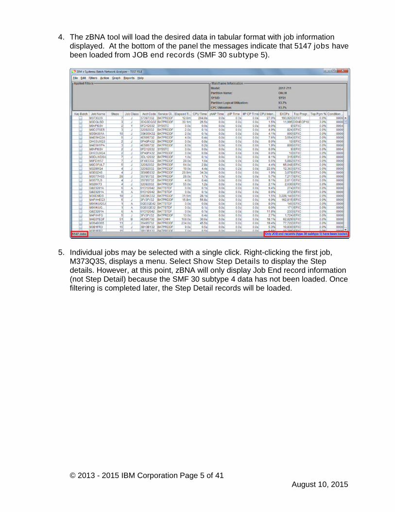
4. The zBNA tool will load the desired data in tabular format with job informationdisplayed. At the bottom of the panel the messages indicate that 5147 jobs havebeen loaded from JOB end records (SMF 30 subtype 5).
5. Individual jobs may be selected with a single click. Right-clicking the first job,M373Q3S, displays a menu. Select Show Step Details to display the Stepdetails. However, at this point, zBNA will only display Job End record information(not Step Detail) because the SMF 30 subtype 4 data has not been loaded. Oncefiltering is completed later, the Step Detail records will be loaded.
© 2013 - 2015 IBM Corporation Page 6 of 41August 10, 2015
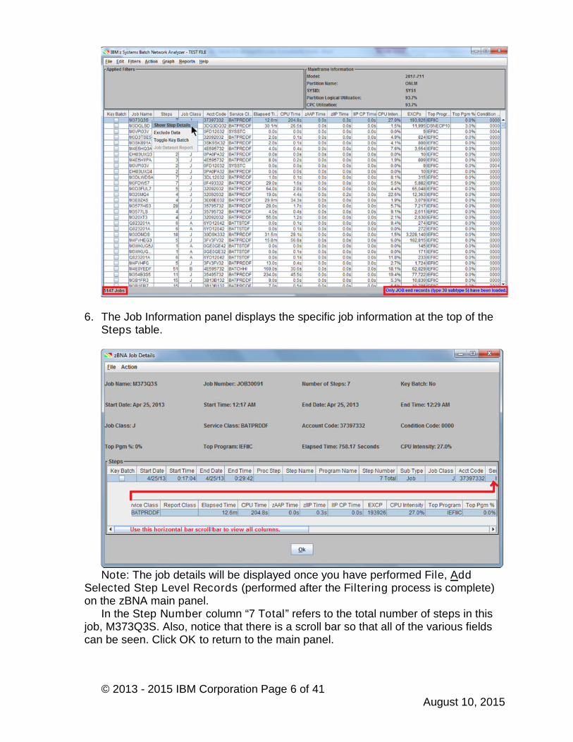
6. The Job Information panel displays the specific job information at the top of theSteps table.
Note: The job details will be displayed once you have performed File, AddSelected Step Level Records (performed after the Filtering process is complete)on the zBNA main panel.
In the Step Number column “7 Total” refers to the total number of steps in thisjob, M373Q3S. Also, notice that there is a scroll bar so that all of the various fieldscan be seen. Click OK to return to the main panel.

© 2013 - 2015 IBM Corporation Page 7 of 41August 10, 2015
7. Jobs may be sorted by any parameter on the screen in both ascending anddescending order, simply by clicking on the corresponding column header. Clickthe CPU Time column twice to sort from the largest to smallest values. Also notethat the number of jobs in the screen, displayed in the bottom left-hand corner, isstill currently 5147 jobs.
© 2013 - 2015 IBM Corporation Page 8 of 41August 10, 2015
Task 2 - Filtering Data
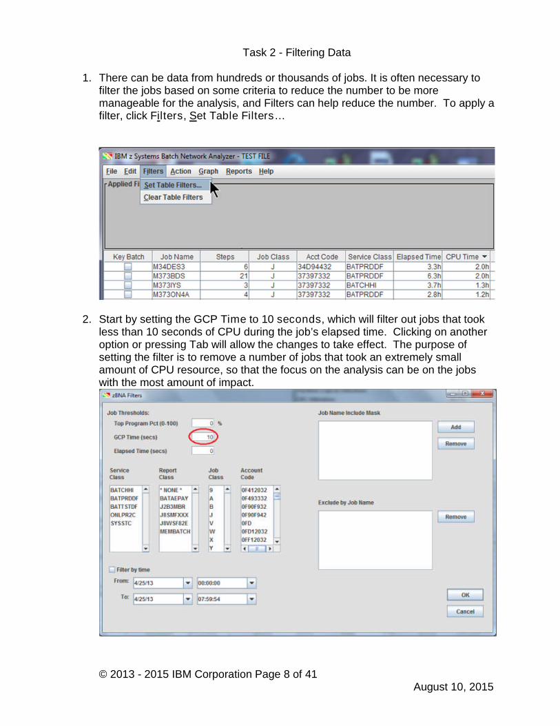
1. There can be data from hundreds or thousands of jobs. It is often necessary tofilter the jobs based on some criteria to reduce the number to be moremanageable for the analysis, and Filters can help reduce the number. To apply afilter, click Filters, Set Table Filters…
2. Start by setting the GCP Time to 10 seconds, which will filter out jobs that tookless than 10 seconds of CPU during the job’s elapsed time. Clicking on anotheroption or pressing Tab will allow the changes to take effect. The purpose ofsetting the filter is to remove a number of jobs that took an extremely smallamount of CPU resource, so that the focus on the analysis can be on the jobswith the most amount of impact.
© 2013 - 2015 IBM Corporation Page 9 of 41August 10, 2015
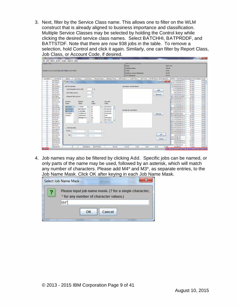
3. Next, filter by the Service Class name. This allows one to filter on the WLMconstruct that is already aligned to business importance and classification.Multiple Service Classes may be selected by holding the Control key whileclicking the desired service class names. Select BATCHHI, BATPRDDF, andBATTSTDF. Note that there are now 938 jobs in the table. To remove aselection, hold Control and click it again. Similarly, one can filter by Report Class,Job Class, or Account Code, if desired.
4. Job names may also be filtered by clicking Add. Specific jobs can be named, oronly parts of the name may be used, followed by an asterisk, which will matchany number of characters. Please add M4* and M3*, as separate entries, to theJob Name Mask. Click OK after keying in each Job Name Mask.
© 2013 - 2015 IBM Corporation Page 10 of 41August 10, 2015
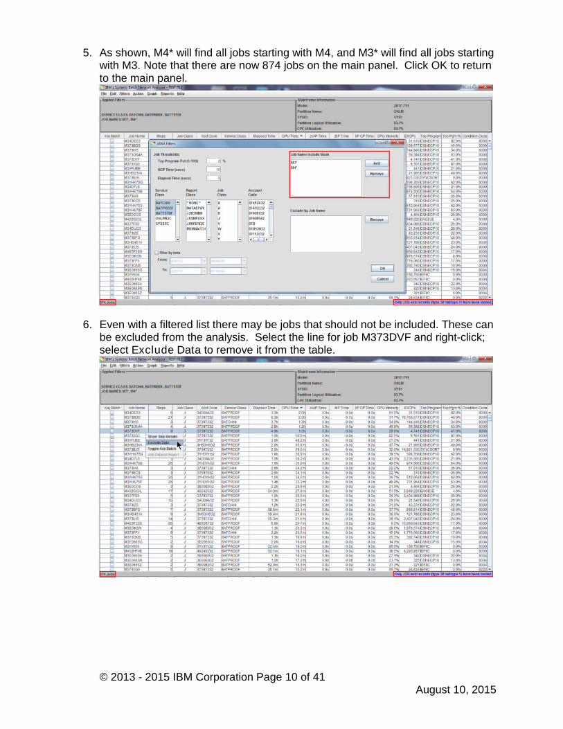
5. As shown, M4* will find all jobs starting with M4, and M3* will find all jobs startingwith M3. Note that there are now 874 jobs on the main panel. Click OK to returnto the main panel.
6. Even with a filtered list there may be jobs that should not be included. These canbe excluded from the analysis. Select the line for job M373DVF and right-click;select Exclude Data to remove it from the table.
© 2013 - 2015 IBM Corporation Page 11 of 41August 10, 2015
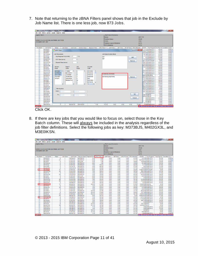
7. Note that returning to the zBNA Filters panel shows that job in the Exclude byJob Name list. There is one less job, now 873 Jobs.
Click OK.
8. If there are key jobs that you would like to focus on, select those in the KeyBatch column. These will always be included in the analysis regardless of thejob filter definitions. Select the following jobs as key: M373BJ5, M402GX3L, andM3E0IKSN.
© 2013 - 2015 IBM Corporation Page 12 of 41August 10, 2015
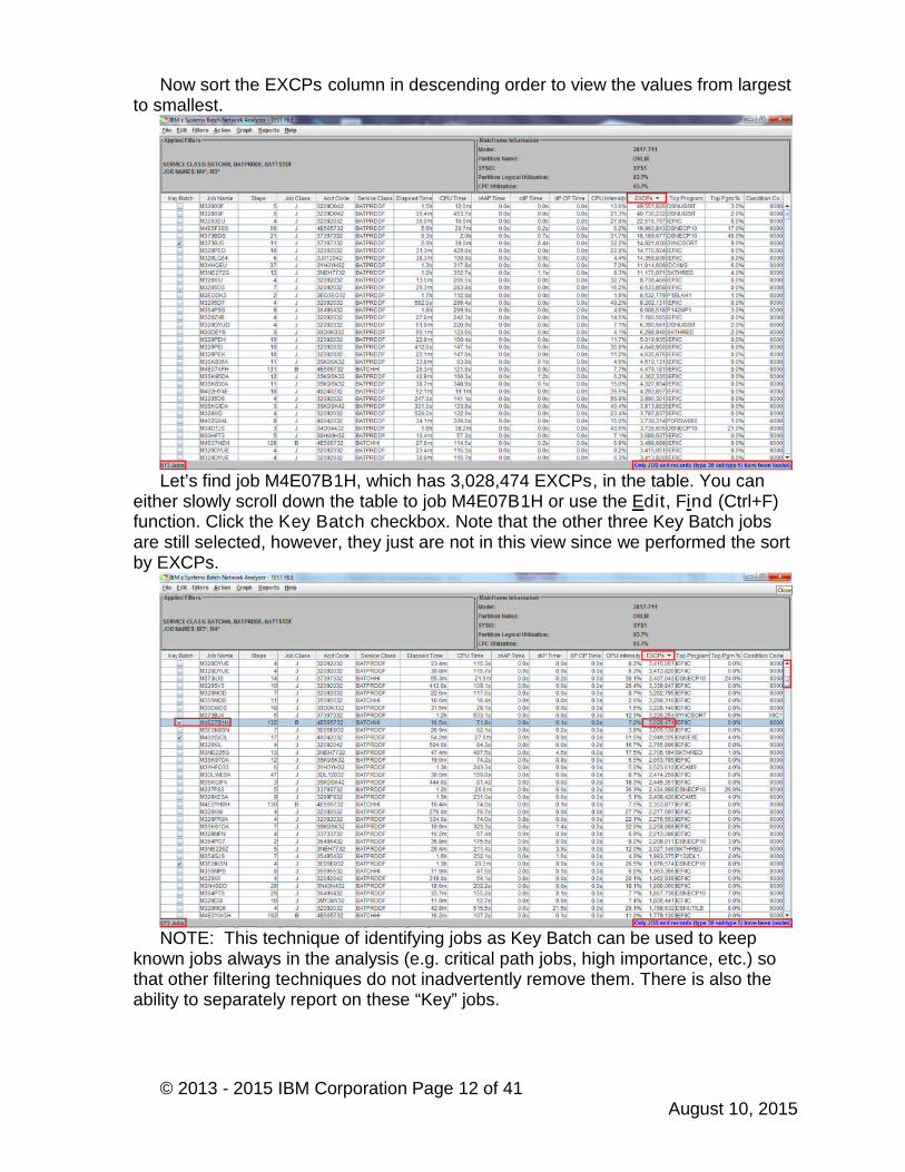
Now sort the EXCPs column in descending order to view the values from largestto smallest.
Let’s find job M4E07B1H, which has 3,028,474 EXCPs, in the table. You caneither slowly scroll down the table to job M4E07B1H or use the Edit, Find (Ctrl+F)function. Click the Key Batch checkbox. Note that the other three Key Batch jobsare still selected, however, they just are not in this view since we performed the sortby EXCPs.
NOTE: This technique of identifying jobs as Key Batch can be used to keepknown jobs always in the analysis (e.g. critical path jobs, high importance, etc.) sothat other filtering techniques do not inadvertently remove them. There is also theability to separately report on these “Key” jobs.
© 2013 - 2015 IBM Corporation Page 13 of 41August 10, 2015
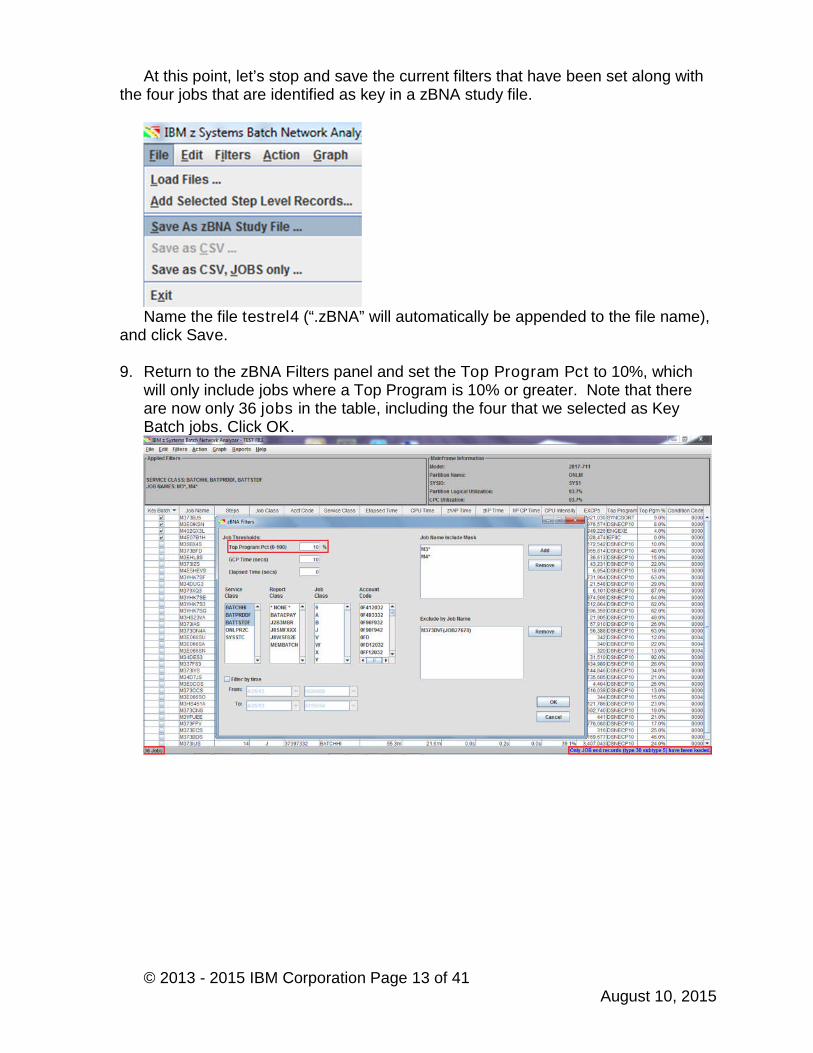
At this point, let’s stop and save the current filters that have been set along withthe four jobs that are identified as key in a zBNA study file.
Name the file testrel4 (“.zBNA” will automatically be appended to the file name),and click Save.
9. Return to the zBNA Filters panel and set the Top Program Pct to 10%, whichwill only include jobs where a Top Program is 10% or greater. Note that thereare now only 36 jobs in the table, including the four that we selected as KeyBatch jobs. Click OK.
© 2013 - 2015 IBM Corporation Page 14 of 41August 10, 2015
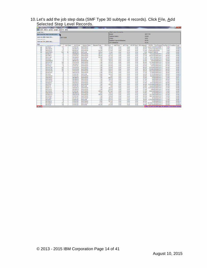
10.Let’s add the job step data (SMF Type 30 subtype 4 records). Click File, AddSelected Step Level Records.

© 2013 - 2015 IBM Corporation Page 15 of 41August 10, 2015
11.The main zBNA panel is redisplayed. Now a job can be drilled down to show thestep level details. (Note that the message “Only JOB end records (type 30subtype 5) have been loaded” is no longer displayed in the information bar).
Let’s sort on the Elapsed Time column so that the longest running job is the firstone displayed in the table.
Job M373BDS is the longest running job in this filtered set. You can see that theelapsed time is 6.3 hours and had 21 Steps. Right click on that job, and selectShow Step Details. Note: Double clicking in the job row will perform the same task.
© 2013 - 2015 IBM Corporation Page 16 of 41August 10, 2015
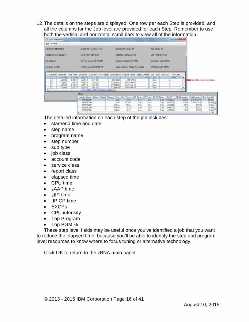
12.The details on the steps are displayed. One row per each Step is provided, andall the columns for the Job level are provided for each Step. Remember to useboth the vertical and horizontal scroll bars to view all of the information.
The detailed information on each step of the job includes: start/end time and date step name program name step number sub type job class account code service class report class elapsed time CPU time zAAP time zIIP time IIP CP time EXCPs CPU intensity Top Program Top PGM %These step level fields may be useful once you’ve identified a job that you want
to reduce the elapsed time, because you’ll be able to identify the step and programlevel resources to know where to focus tuning or alternative technology.
Click OK to return to the zBNA main panel.
© 2013 - 2015 IBM Corporation Page 17 of 41August 10, 2015
Task 3 – Displaying a Graph
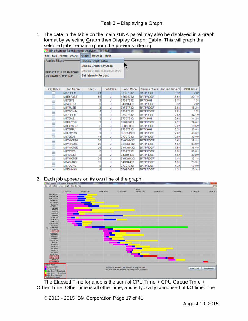
1. The data in the table on the main zBNA panel may also be displayed in a graphformat by selecting Graph then Display Graph: Table. This will graph theselected jobs remaining from the previous filtering.
2. Each job appears on its own line of the graph.
The Elapsed Time for a job is the sum of CPU Time + CPU Queue Time +Other Time. Other time is all other time, and is typically comprised of I/O time. The

© 2013 - 2015 IBM Corporation Page 18 of 41August 10, 2015
sum of the 3 components is placed on the X axis when the Job’s Elapsed Timeoccurred in the interval, but they represent the % of time spent in each component(e.g. the actual CPU Time does not all occur at the beginning of the job).
The legend for the graph appears in the bottom left corner. Pink, Execution (CPU Time, shows the measured CPU time for a job. Blue, CPU Queue Time, represents the estimated CPU wait time for a
job, which is calculated from the RMF Service class waiting for dispatchfield.
Other Time, a green bar signifies that the job’s CPU execution time is lessthan 10% (default value for Set Intensity Percent) of the job’s duration.
Other Time, a yellow bar signifies that the CPU execution time is morethan 10% (default value for Set Intensity Percent) of the duration.
Other Time, a red bar signifies Key batch jobs.
3. Clicking and dragging an area on the graph will zoom the graph in to that area.

© 2013 - 2015 IBM Corporation Page 19 of 41August 10, 2015
4. Holding Control allows the user to pan across the graph. The cursor will becomea cross when this is happening.
Click Reset Graph to show the original graph.
5. Hold the mouse over a job to show the Job information.
Further detail is available for each job by right-clicking and selecting Show StepDetails. Right-click M373BJ5 (the first Key job with Red Other time) and click ShowStep Details.

© 2013 - 2015 IBM Corporation Page 20 of 41August 10, 2015
6. The same Job Step panel that is accessible from the main panel displays.
Click OK to return to the graph.
© 2013 - 2015 IBM Corporation Page 21 of 41August 10, 2015
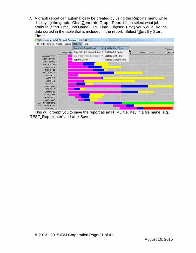
7. A graph report can automatically be created by using the Reports menu whiledisplaying the graph. Click Generate Graph Report then select what jobattribute (Start Time, Job Name, CPU Time, Elapsed Time) you would like thedata sorted in the table that is included in the report. Select “Sort By StartTime”.
This will prompt you to save the report as an HTML file. Key in a file name, e.g.“TEST_Report.htm” and click Save.
© 2013 - 2015 IBM Corporation Page 22 of 41August 10, 2015
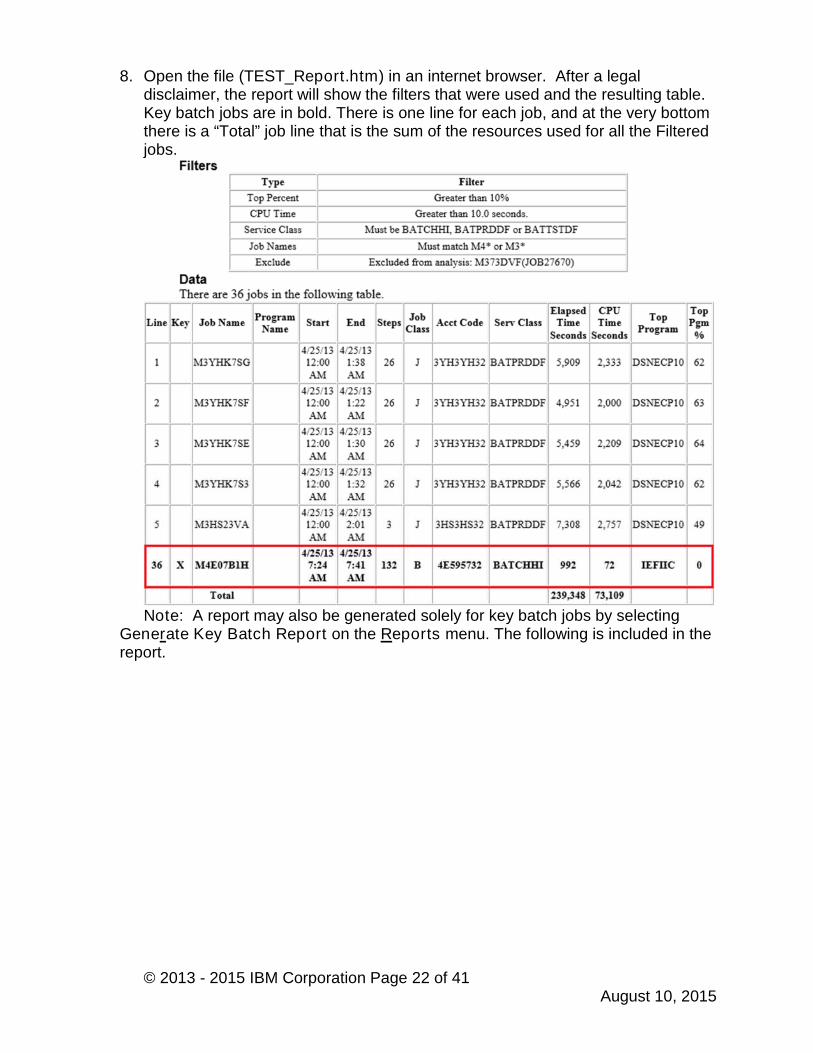
8. Open the file (TEST_Report.htm) in an internet browser. After a legaldisclaimer, the report will show the filters that were used and the resulting table.Key batch jobs are in bold. There is one line for each job, and at the very bottomthere is a “Total” job line that is the sum of the resources used for all the Filteredjobs.
Note: A report may also be generated solely for key batch jobs by selectingGenerate Key Batch Report on the Reports menu. The following is included in thereport.

© 2013 - 2015 IBM Corporation Page 23 of 41August 10, 2015
9. When the graph report is initially generated, the graph is not present. To includethe graph in the report, click Reports, Append Graph. You will be prompted toselect the previously saved report file. Then click Save, and the graph will beappended to the report.
Click Back to Main to return to the zBNA main panel.
© 2013 - 2015 IBM Corporation Page 24 of 41August 10, 2015
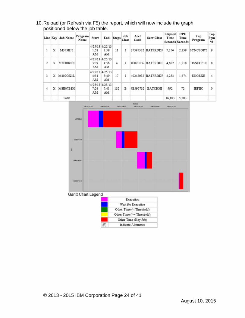
10.Reload (or Refresh via F5) the report, which will now include the graphpositioned below the job table.
© 2013 - 2015 IBM Corporation Page 25 of 41August 10, 2015
Task 4 – Reviewing DASD Data Set Information
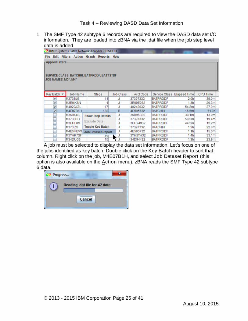
1. The SMF Type 42 subtype 6 records are required to view the DASD data set I/Oinformation. They are loaded into zBNA via the .dat file when the job step leveldata is added.
A job must be selected to display the data set information. Let’s focus on one ofthe jobs identified as key batch. Double click on the Key Batch header to sort thatcolumn. Right click on the job, M4E07B1H, and select Job Dataset Report (thisoption is also available on the Action menu). zBNA reads the SMF Type 42 subtype6 data.

© 2013 - 2015 IBM Corporation Page 26 of 41August 10, 2015
2. The zBNA Job Dataset Report panel displays the data sets for job M4E07B1H.
Be sure to use the scroll bars to get a complete view of the job details. Sort theTotal IO Time column in descending order so that the data set with the most IO timeis positioned in the first row.
3. Right click on I4E5SEY.M4E57B1S.SOQDVSG.LQGHA, and select Get the Lifeof this Dataset.

© 2013 - 2015 IBM Corporation Page 27 of 41August 10, 2015
4. zBNA reads the .dat file that is loaded for the SMF 42 then the SMF 30 data. Itsearches through all Jobs (5147), not just the Filtered Jobs. When it finishes theprocess, the zBNA: Life of a Dataset panel is displayed.
The job names using this data set are shown. Use the scroll bar to view all of thedata, and the columns can be sorted.
In this case, Job M4E07B1H is the only job that accessed the data set; in Steps88 and 92. Step 92 has the most Total IO Time, 188 seconds. The response time isvery low. If you scroll to the right, in the column Type, you’ll see it is a “KSDSIndex”. While not currently provided in zBNA, one could investigate SMF 64s andconsider increasing LSR / NSR buffers to hold Index Set and potentially eliminate ~3Minutes of I/O time, which would be approximately 18% of the Job’s elapsed time(16.5 minutes).
Click OK until the zBNA main panel is displayed.
© 2013 - 2015 IBM Corporation Page 28 of 41August 10, 2015
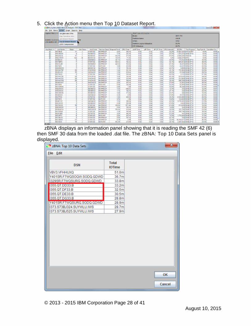
5. Click the Action menu then Top 10 Dataset Report.
zBNA displays an information panel showing that it is reading the SMF 42 (6)then SMF 30 data from the loaded .dat file. The zBNA: Top 10 Data Sets panel isdisplayed.

© 2013 - 2015 IBM Corporation Page 29 of 41August 10, 2015
The purpose is to show where the most I/O time is, over the entire interval andregardless of who is accessing the dataset. Then looking at the characteristics,technology options can be evaluated to improve the response time, and thus theelapsed times of the jobs/online applications that are accessing it. In this case, itappears that 4 data sets starting with I335.QT. are the 4th through 7th Top data sets.Perhaps they are clones that we enabled for parallel processing? We’ll investigateone of these files.
6. The Top 10 data sets are displayed, and the information can be written to a CSVfile when you select the option on the File menu.
Right click on the I355.QT.DD33.B data set then Get the Life of this Dataset.After zBNA reads the SMF 42 and 30 data in the .dat file, the zBNA: Life of aDataset panel is displayed.
© 2013 - 2015 IBM Corporation Page 30 of 41August 10, 2015
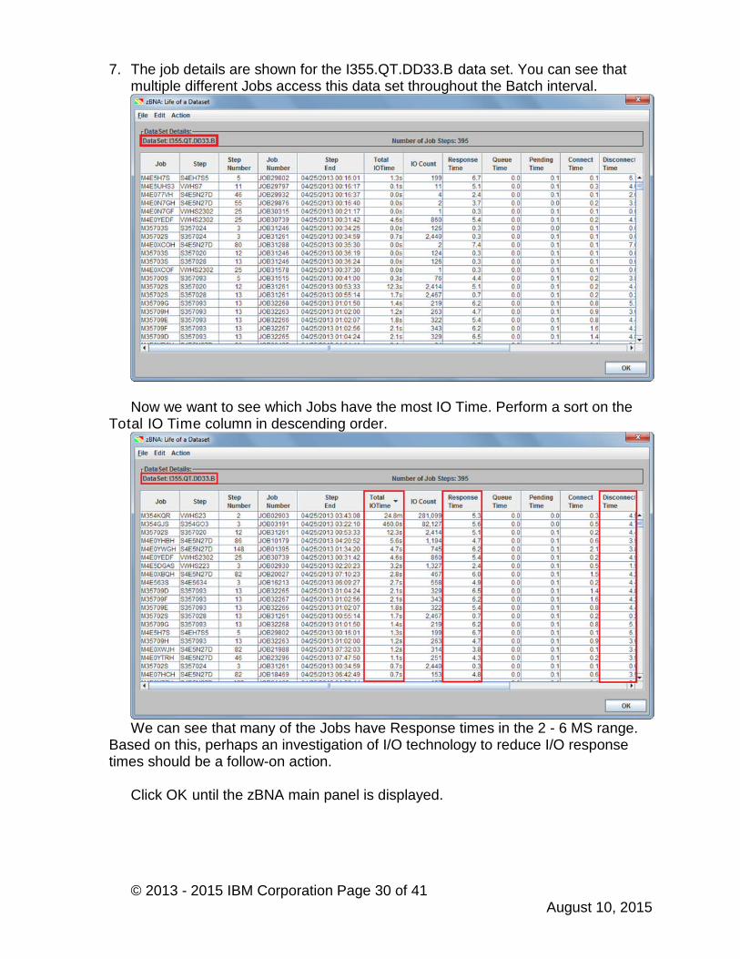
7. The job details are shown for the I355.QT.DD33.B data set. You can see thatmultiple different Jobs access this data set throughout the Batch interval.
Now we want to see which Jobs have the most IO Time. Perform a sort on theTotal IO Time column in descending order.
We can see that many of the Jobs have Response times in the 2 - 6 MS range.Based on this, perhaps an investigation of I/O technology to reduce I/O responsetimes should be a follow-on action.
Click OK until the zBNA main panel is displayed.
© 2013 - 2015 IBM Corporation Page 31 of 41August 10, 2015
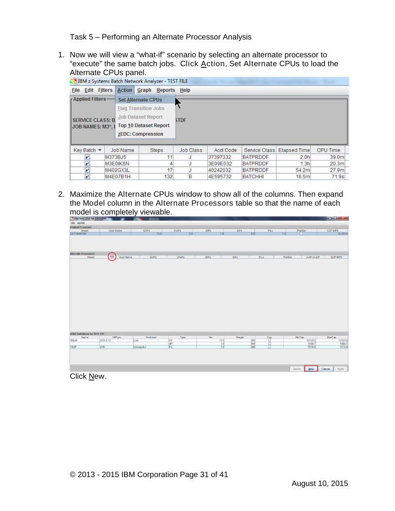
Task 5 – Performing an Alternate Processor Analysis
1. Now we will view a “what-if” scenario by selecting an alternate processor to“execute” the same batch jobs. Click Action, Set Alternate CPUs to load theAlternate CPUs panel.
2. Maximize the Alternate CPUs window to show all of the columns. Then expandthe Model column in the Alternate Processors table so that the name of eachmodel is completely viewable.
Click New.
© 2013 - 2015 IBM Corporation Page 32 of 41August 10, 2015
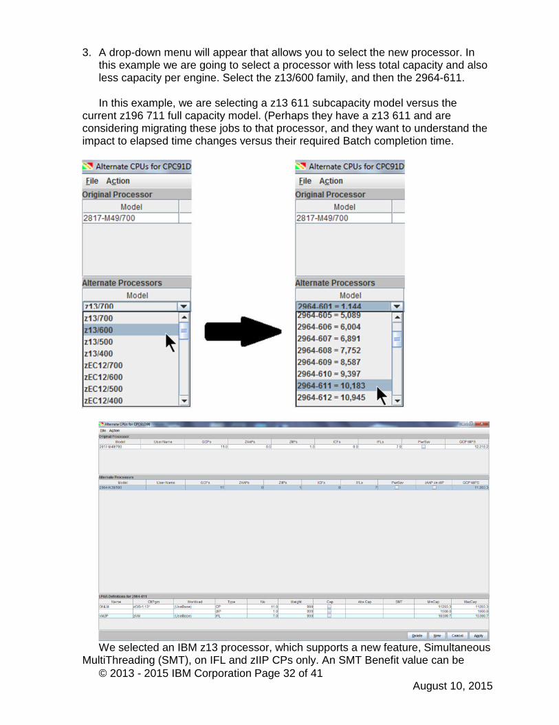
3. A drop-down menu will appear that allows you to select the new processor. Inthis example we are going to select a processor with less total capacity and alsoless capacity per engine. Select the z13/600 family, and then the 2964-611.
In this example, we are selecting a z13 611 subcapacity model versus thecurrent z196 711 full capacity model. (Perhaps they have a z13 611 and areconsidering migrating these jobs to that processor, and they want to understand theimpact to elapsed time changes versus their required Batch completion time.
We selected an IBM z13 processor, which supports a new feature, SimultaneousMultiThreading (SMT), on IFL and zIIP CPs only. An SMT Benefit value can be
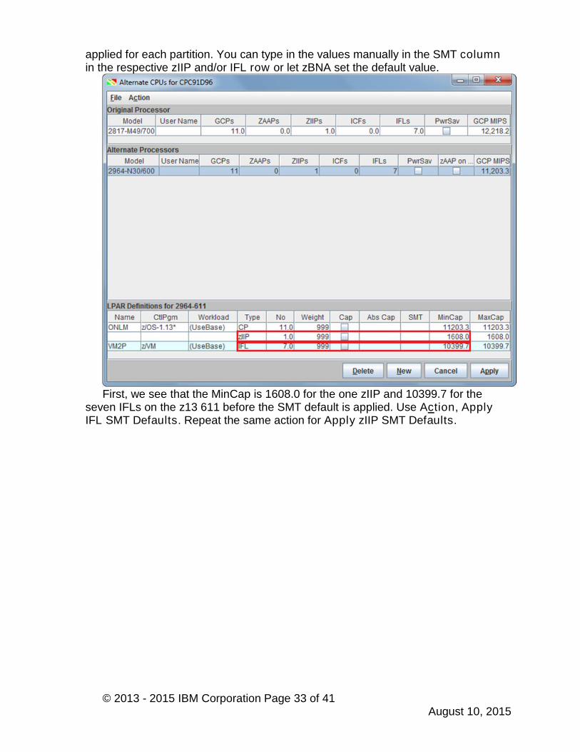
© 2013 - 2015 IBM Corporation Page 33 of 41August 10, 2015
applied for each partition. You can type in the values manually in the SMT columnin the respective zIIP and/or IFL row or let zBNA set the default value.
First, we see that the MinCap is 1608.0 for the one zIIP and 10399.7 for theseven IFLs on the z13 611 before the SMT default is applied. Use Action, ApplyIFL SMT Defaults. Repeat the same action for Apply zIIP SMT Defaults.

© 2013 - 2015 IBM Corporation Page 34 of 41August 10, 2015
The suggested default SMT Benefit values are 25% for zIIP CPs and 20% forIFL CPs. You can see the increased MinCap values after applying SMT. Click Applyto view the hypothetical scenario with this new processor.
© 2013 - 2015 IBM Corporation Page 35 of 41August 10, 2015
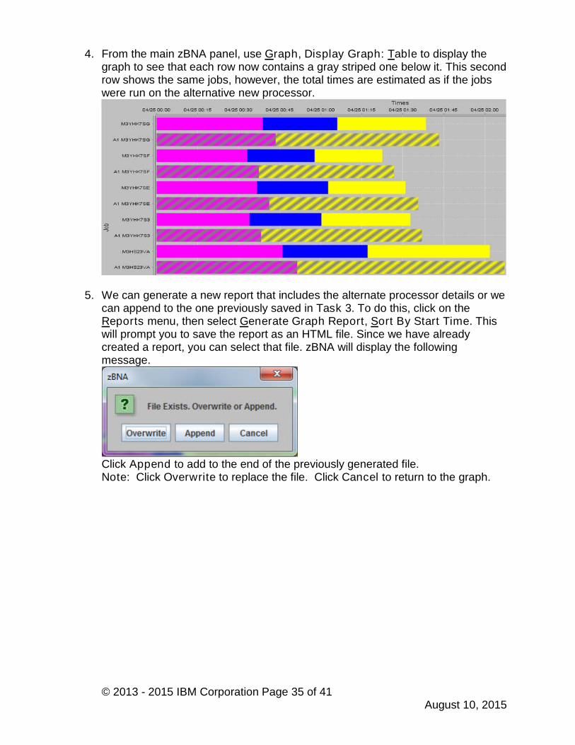
4. From the main zBNA panel, use Graph, Display Graph: Table to display thegraph to see that each row now contains a gray striped one below it. This secondrow shows the same jobs, however, the total times are estimated as if the jobswere run on the alternative new processor.
5. We can generate a new report that includes the alternate processor details or wecan append to the one previously saved in Task 3. To do this, click on theReports menu, then select Generate Graph Report, Sort By Start Time. Thiswill prompt you to save the report as an HTML file. Since we have alreadycreated a report, you can select that file. zBNA will display the followingmessage.
Click Append to add to the end of the previously generated file.Note: Click Overwrite to replace the file. Click Cancel to return to the graph.

© 2013 - 2015 IBM Corporation Page 36 of 41August 10, 2015
6. The report will now include the alternate processor, as well as the estimated run-time in the table for this new processor.
In this case we can see that the Alternate Processor had a Ratio of -8.3% SingleGCP MIPS, resulting in slightly increased CPU and Elapsed times compared to thecurrent processor for each job.
7. Let’s save the study as a zBNA file, click File, Save As zBNA Study File. Thissaves a .zBNA file containing the current filters and settings including the keybatch jobs. However, when you load the .zBNA file, the original SMF70 andSMF30 files will still be needed.
© 2013 - 2015 IBM Corporation Page 37 of 41August 10, 2015
Task 6 – Exploring zEDC Compression
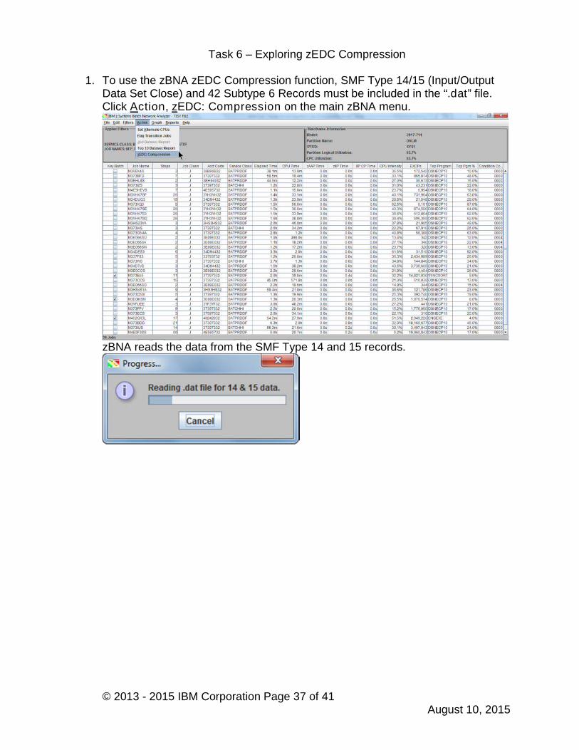
1. To use the zBNA zEDC Compression function, SMF Type 14/15 (Input/OutputData Set Close) and 42 Subtype 6 Records must be included in the “.dat” file.Click Action, zEDC: Compression on the main zBNA menu.
zBNA reads the data from the SMF Type 14 and 15 records.

© 2013 - 2015 IBM Corporation Page 38 of 41August 10, 2015
2. The zEDC Top Data Sets panel displays after the SMF Type 14, 15, 42(6)records have been loaded.
These are the data sets that zBNA has calculated are the top zEDCCompression candidates. Note: By default, the list is ordered by the top data sets,according to MB.
The purpose of providing the Top Data Sets is to identify which ones will providethe most impact/benefit from zEDC compression, and may provide a starting pointfor which ones to implement first.
Notes: You can drill down further on a data set by right clicking on its name and
selecting Get the Life of this Dataset. Right click on a specific data set, and select zEDC Dataset Analysis to
see the job and steps associated with that data set. All of the data sets in the table can be selected at once. Right click in the
check box column, Select All. An option, Clear All, is available.
© 2013 - 2015 IBM Corporation Page 39 of 41August 10, 2015
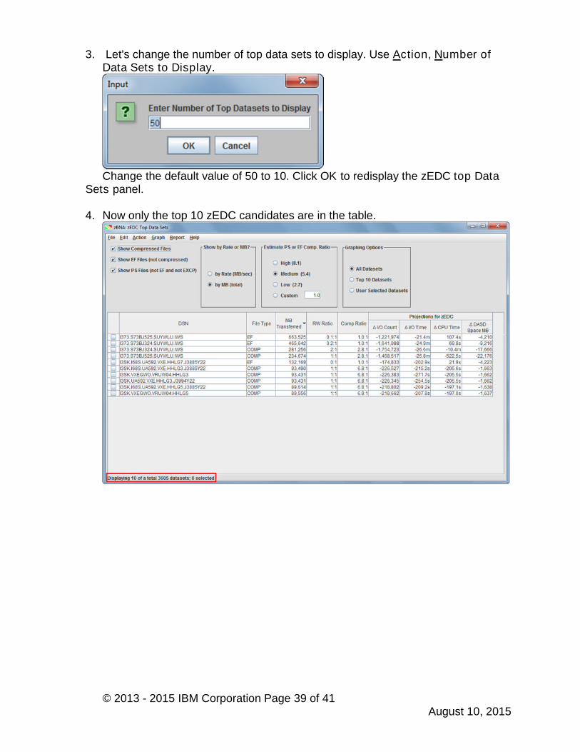
3. Let's change the number of top data sets to display. Use Action, Number ofData Sets to Display.
Change the default value of 50 to 10. Click OK to redisplay the zEDC top DataSets panel.
4. Now only the top 10 zEDC candidates are in the table.

© 2013 - 2015 IBM Corporation Page 40 of 41August 10, 2015
5. Let's look a few of the zEDC graphs. Click Graph, Projected zEDC Cards.
This graph shows the estimated number of zEDC cards by hour needed tosupport the workload for all data sets that met the criteria in the interval. With thisgraph you can see the peak time and how many cards are required from a capacityperspective. Save this data and graphic image to a zBNA report file by clickingReport, Output Graph. Input “zEDCgraph” for the file name, and click Save. Boththe “.htm” and “.jpg” files are generated.
6. Click Graph, Projected zEDC CPU Savings.
© 2013 - 2015 IBM Corporation Page 41 of 41August 10, 2015
This graph shows the projected zEDC CPU Savings by file type. Compressedhas the largest savings, as the CPU will be offloaded to the zEDC card. Save andappend this graphic image to the zEDCgraph.htm file that was created. A ".jpg" fileis created and saved in the updated ".htm" file.
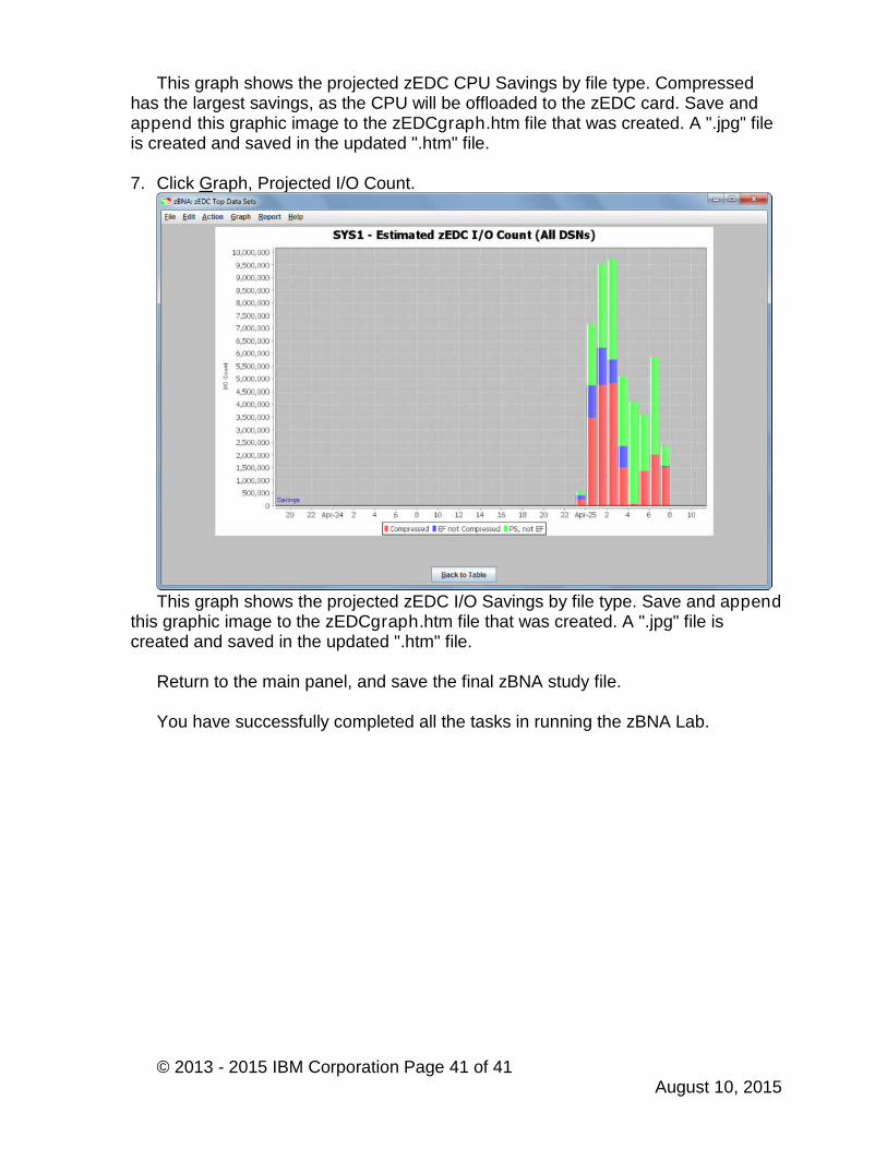
7. Click Graph, Projected I/O Count.
This graph shows the projected zEDC I/O Savings by file type. Save and appendthis graphic image to the zEDCgraph.htm file that was created. A ".jpg" file iscreated and saved in the updated ".htm" file.
Return to the main panel, and save the final zBNA study file.
You have successfully completed all the tasks in running the zBNA Lab.