Zeiss 880 (inverted) Confocal/Multiphoton Microscope User Guide B45D Weill Hall

2

TABLE OF CONTENTS

PAGE Starting the Zen software 3 Locate 4 Acquisition 5 Laser 6 Smart Setup 6 Light Path 8 Setting up a configuration manually 9 Acquisition Mode 9 Channels 11 Image acquisition 12 Image optimization - Range Indicator 12 Image optimization - Adjust laser intensity 13 Image optimization – Adjust gain and offset 13 Zoom – Live 13 Zoom – Crop box 14 Reuse 14 Image Display 14 Saving images 15 Scanning a Z stack – First/Last Mode 16 Center option for Z series 17 Center mode: Z stack at several positions 17 Scanning a Time Series 17 Tile Scan 18 Tile Scan – selecting positions 18 Bleaching (Photobleaching, FRAP/Photoactivation) 20 Positions or Multi x-y-z 21 Focus 21 Stage 21 Reflected Light Confocal 22 Transmitted Light (Brightfield) 22 Lambda Mode 23 Multiphoton (LSM or Confocal Mode) 25 Multiphoton (Non-Descanned Detection) 27

3

Starting the ZEN software

• Double click the ZEN icon on the WINDOWS desktop • The ZEN Main Application window and the LSM 880 Startup window appear on

the screen • In the small startup window, choose either to start the system (Start System

hardware for acquiring new images) or in Image Processing mode to edit already existing images. Toggle the little arrow symbol to view the Boot Status display.

• After Startup, the ZEN Main Application Window opens.

• On the Left Tool Area, the user finds the tools for sample observation, image acquisition, image processing and system maintenance, easily accessible via the five Main Tabs (Locate, Acquisition, FCS, Processing, and Maintain).

• All functions needed to control the microscope can be found on the Locate Tab; to acquire images use the Acquisition Tab

4

LOCATE

View sample through microscope eyepieces using either a halogen lamp or mercury halide lamp source; focus, and locate region to image

• Click on the

objective icon to select objective lens (magnification, numerical aperture [NA], immersion)

• Click on either the

Brightfield or Fluorescence buttons to turn on lamps and view sample thru eyepieces

• For Fluorescence, click on filter icon to select filter to view specimen fluorescence

• To turn light source off,

Brightfield: click Off button next to Transmitted Light Fluorescence: click Off button next to Reflected Light Or just close the appropriate Shutter!

• Incubator blue tool bar – for temperature and CO2 control

• When ready to do confocal, click on Acquisition Tab

BRIGHTFIELD FLUORESCENCE

5

ACQUISITION

• Make sure Show all Tools box is checked

• Click on blue tool panels to view/hide items

• Activate Show all by hitting View on the main menu, then click on Show all (global)

The Show all concept ensures that tool panels are never more complex than needed. With Show all deactivated, the most commonly used tools are displayed. For each tool, the user can activate Show all mode to display and use additional functionality.

Tools: • Laser – manual turn on/off

of lasers; view properties of highlighted laser

• Light Path – Imaging modes; diagram of excitation and emission light path of fluorophores

• Acquisition Mode – imaging parameters

• Channels – laser power, detector and pinhole settings

• Focus and Stage – adjustments through software

• Focus Devices and Strategy – autofocus • Shuffle and Find – locating marked areas of specimen

6

Laser

If needed, turn on the Argon multi-line laser. The laser is first highlighted in red (turning on), then goes on Standby (warming up ~5 min). It turns ON when ready.

The multiphoton lasers include a fixed line at 1040 nm and a tunable line from 680-1300. Highlighting the Tunable laser and clicking on Laser Properties shows the current wavelength of the tunable laser.

Smart Setup

The tool Smart Setup is an intuitive, user-friendly interface which can be used for almost all standard applications. It configures all the system hardware for a chosen set of dyes.

• Click on the Smart Setup button to open the Smart Setup window. This window can be accessed any time from the software to change dye combinations.

7

• Click on the arrow

in the Dye list and choose the dye(s) you want to use from the list dialogue. In this dialogue, the dyes can be also searched by typing the name in the search field.

• Once finished

with the input, Smart Setup suggests alternative considerations: One for Fastest imaging, one for the Best signal, and another for Smartest (compromise between both speed and best signal), and sometimes the optimal setup for later Linear Unmixing of the dyes is also displayed.

The graphs display relative values for the expected emission signals and cross-talk. The resulting imaging scheme (single or multitrack) is shown below the graphs.

• Pressing Apply, automatically sets the hardware parameters in the displayed way for the dyes chosen. If the option Linear Unmixing is selected, the system is set in the lambda mode automatically. The dyes chosen are displayed in the Light Path tool tab.

Note: The smart setup path does NOT necessarily assign the fluorophores chosen to the optimal detector for the emission wavelength of the chosen fluorophores. Specifically, fluorophores with wavelengths in the middle of the visible light spectrum may NOT be assigned to the higher sensitivity GaAsP detector.

8

Light Path

The Light Path tool displays the selected track configuration which is used for the scan procedure. You can change the settings of this panel using the following function elements:

• Main dichroic beam splitter (MBS) for visible and invisible light from the relevant list box

• Spectral emission range detected: adjust horizontal sliders underneath displayed spectra

• Activate/deactivate (via check box) selected channel for the scanning procedure; assign a color to the channel.

• Laser icon: to select the laser lines and set the attenuation values (transmission in %) in the displayed window.

• Detection Bands & Laser Lines are displayed in a spectral panel to visualize the activated laser lines for excitation (vertical lines) and activated detection channels (colored horizontal bars).

Ch1 and Ch2 are standard alkali PMTs. ChS1 is an array of 32 high-sensitivity GaAsP PMTs.

This can use up to 8 channels in Channel mode (but they have to have the same gain at any time, but different digital gain is allowed).

• If you have created a configuration, either manually or via Smart Setup, you can save

this in the Experiment Manager for easy reloading in the future.

9

Setting up a configuration manually: Tracks

• Simultaneous scanning of single, double and triple labeling (uses 1 Track): faster image acquisition, but potential cross-talk between channels

• Sequential scanning of double and triple labeling; line-by-line or frame-by-frame (uses 2 or more Tracks): only one detector and one laser are switched on at any one time. This reduces crosstalk, but image acquisition is slower

A maximum of four tracks with up to eight channels can be defined simultaneously and then scanned one after the other. Each track is a separate unit and can be configured independently from the other tracks with regard to channels, spectral emission, dichroic beam splitters and pinhole settings. • Switch track every Line: Tracks are switched during scanning line-by-line. The

following settings can be changed between tracks: Laser line, laser intensity and channels.

• Switch track every Frame: Tracks are switched during scanning frame-by-frame. The following settings can be changed between tracks: Laser line and intensity, all filters and beam splitters, the channels incl. settings for gain and offset and the pinhole position and diameter.

• Add Track (+): An additional track is added to the configuration list in the Imaging

Setup Tool. A maximum of 4 tracks can be used. • Remove Track (trash): The track marked in the List of Tracks panel is deleted.

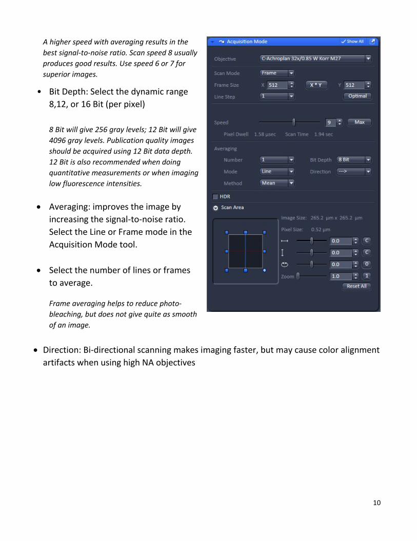
Acquisition Mode: Setting the parameters for scanning

• Scan Mode: Frame or Line • Frame Size: default is 512 x 512 pixels; Click on X*Y button to select a different frame

size; Click on the Optimal button for calculation of appropriate number of pixels depending on objective N.A. and λ.

The number of pixels influences the image resolution!

• Speed: Use the scan speed slider to adjust the scan speed

10

A higher speed with averaging results in the best signal-to-noise ratio. Scan speed 8 usually produces good results. Use speed 6 or 7 for superior images.

• Bit Depth: Select the dynamic range 8,12, or 16 Bit (per pixel)

8 Bit will give 256 gray levels; 12 Bit will give 4096 gray levels. Publication quality images should be acquired using 12 Bit data depth. 12 Bit is also recommended when doing quantitative measurements or when imaging low fluorescence intensities.

• Averaging: improves the image by increasing the signal-to-noise ratio. Select the Line or Frame mode in the Acquisition Mode tool.

• Select the number of lines or frames to average. Frame averaging helps to reduce photo-bleaching, but does not give quite as smooth of an image.

• Direction: Bi-directional scanning makes imaging faster, but may cause color alignment artifacts when using high NA objectives

11

Channels

• Image optimization via adjustments of laser power, pinhole size, detector gain and offset.

• Set the Pinhole size to 1 AU (Airy unit) for best compromise between depth discrimination and detection efficiency.

Pinhole adjustment changes the Optical Slice thickness. When collecting multi-track, multi-channel images, adjust the pinholes so that each channel has the same Optical Slice thickness. This is important for colocalization studies.

• Ch2 and ChS detectors can be used to image samples via Integration or Photon Counting Mode. The latter is only recommended for very weak fluorescence signals.

• To view all channels under various tracks, click on Expand All.

12

Image acquisition

Use one of the Set Exposure, Live, Continuous or Snap buttons to start the scanning procedure to acquire an image. A clicked button changes to a Stop button when scanning. Scanned images are shown in separate windows.

• Select Set Exposure for automatic pre-adjustment of detector gain and offset. • Select Live for continuous fast scanning – useful for finding and changing the focus. • Select Continuous for continuous scanning with the selected scan speed and

averaging. • Select Snap for recording a single image. • Select Stop for stopping the current scan procedure.

Image optimization

Choose Range Indicator

• In the Dimensions tab

located below the image field, click inside the color field in the button under the channel button.

Clicking on the down arrow on the right hand side of the button leads to a list of colors.

13

The scanned image appears in a false-color presentation.

• If the image is too bright, it appears red on the screen. Red = saturation (maximum).

• If the image is not bright enough, it appears blue on the screen. Blue = zero (minimum).

Adjust the laser intensity

• Set the Pinhole to 1 Airy Unit. • Set the Gain (Master) high. • When the image is saturated, reduce AOTF transmission in the Laser control section

of the Channels Tool using the slider to reduce the intensity of the laser light to the specimen.

Adjust gain and offset

• Increase the Digital Offset until all blue pixels disappear, and then make it slightly positive (stay as close as possible to zero)

• Reduce the Gain (Master) until the red pixels only just disappear

Zoom: Live

• Active while live scanning • Adjust zoom value • Move, resize, rotate using

graphic, values, slider, or the small up/down arrows

• Reset All to return to zoom 1 and center of Scan Area

You can zoom out to 0.6 but the corners and edges may be less bright Zoom: Real optical zoom, resolution increases, image area decreases. To image a larger field with small pixels, switch to a larger frame size (eg. 1024 x 1024 pix).

14

Zoom: via Crop Box

• You must stop scanning to use

• Under the Dimensions control block, select Crop

• Position box that appears in image display on object of interest

• Resize, move, rotate • Scan Live to see

zoomed image Reuse

Clicking the Reuse button transfers ALL acquisition parameters (exception: objective and collimator) from stored image data to the Microscope Hardware Settings / Control Tools and applies those parameters directly to the system.

Image Display

To the left of the image container, one can select how the image acquired is displayed: 2D − displays a single image in frame mode, or a multiple channel image in superimposed mode. Split – displays the individual channels of a multi-channel image as well as the superimposed image. 2.5D – This function allows to display the two-dimensional intensity distribution of an image in a pseudo 3D mode, shows the intensity values in profile, grid or filled mode, as well as separate distribution for each channel in a multi-channel image. Histogram – displays a histogram (distribution of pixel intensities) of an image or Region of Interest, shows the histogram values in table form; allows one to copy table to clipboard or save as text file, and to measure area and mean gray value and standard distribution in an area.

15

Profile – displays the intensity distribution of an image along a straight or curved line; shows the intensity values in table form and copy table to clipboard or save as text file; shows separate profiles for each channel in a multi-channel image.

Saving Images

• To save your acquired or processed images, click on the Save or Save As button in File Menu, or click the Save icon in the Main Toolbar, or click on the Save icon at the bottom of the File Handling Area (located at the right side of main application window).

• To export image display data, a single optical section in raw data format or the contents of the image display window including analysis and overlays, choose Export from the File menu. In the Export window you can select from a number of options and proceed to the WINDOWS Save As window to save the exported data to disk.

Remember, an unsaved 2D image in the active image tab will be over-written by a new scan. Multi-dimensional scans (z-stack, time series, etc.) or saved images will never be over-written and a new scan will then automatically create a new image document.

• Save files as .czi. This ensures that all hardware settings are saved and can be reused for future imaging sessions.

• Acquired data is not automatically saved to disc. Make sure you save your data appropriately and back it up regularly. The ZEN software will ask you if you want to save your unsaved images when you try to close the application with unsaved images still open.

• Copy saved images to Z: Imaging Lab FileShare.

16

Scanning a Z stack

• Select Z-Stack in the main tools area. • Open the Z Stack tool in the Left Tool

Area under Multidimensional Acquisition

First/Last Mode:

• Select Mode First/Last on the top of the Z-Stack tool.

• Scan Live. Use the focus drive of the microscope (or focus knob on touchscreen monitor) to focus on the upper position of the specimen area where the Z Stack is to start. Click on the Set First button to set the upper position of the Z Stack.

• If you wish to zero the first position, go to the Focus tab, and click on Manually.

• Focus on the lower specimen area where the recording of the Z Stack is to end. Click on the Set Last button to set this lower position.

• Click on the Smallest button to set number of slices to match the optimal Z-interval for the given stack size, objective lens, and the pinhole diameter.

• Click on the Start Experiment button to start the recording of the Z-Stack.

17

Center Option for Z-series

• Choose Center vs First/Last • Manually focus to the center of sample • Hit Center button • Choose Interval, then calculate the # of

steps needed to get the distance you want and set steps/slices

• Use the focus window to set the center to zero, if desired

Range Select

Will do x-z scan, you can change center or top/bottom on this image

Center Mode: z stack at several positions

• Use the center option to define the z-stack at the first position • Then just add each location (Positions) when in the center of the object. • You must do the same range and step size for each position • X-Y-Z coordinate is recorded • Software sets an offset to relate to center of the first position

Scanning a Time Series

• Select Time series in the main tools area. • Open the Time series tool in the Left Tool

Area under Multidimensional Acquisition • Set Interval and total number of scans

(Cycles): An interval time shorter than the scan time for a frame or line is not effective.

• Click on the Start Experiment button to start the recording of the time series

• If you also have Z-Stack checked, you will get an xyzt series • Definite Focus will keep sample in focus over time

18

Tile Scan

• Select Tile Scan in the main tools area. • Open the Tile Scan tool in the Left Tool

Area under Multidimensional Acquisition

Centered grid (The current position will be the center of the tile scan): Set number of tiles in horizontal and vertical direction

• Scan overview image for quick view • You can do a z-stack at each tile, setup

as usual • When Bi-directional is active, the image

acquisition is performed also on the horizontal backwards movement of the stage.

• Click on the Start Experiment button to start the recording of the tile scan

• Online stitching is possible when a value is put in the Overlap box. A good value to start with is 10%.

Bounding grid or Convex Hull: Positions that should be part of the tile scan have to be marked using Add. Using these positions a bounding grid or convex hull is created, which finally defines the dimensions of the tile scan.

You can select positions on a tiled image and scan selected position.

• Click the Positions button in the Dimensions tab located below the Image display

• Click on the area(s) of the tiled image you want to go to: areas are marked with a white cross and a number

• Go to the Stage tab (blue tab). Positions marked on your tiled image appear under Marks.

• Select the marked position and click the Move to button. Scan.

19

• You can also use the Stage button in the Dimensions tab to select stage positions (areas) in tiled image. A white box with a number appears on the selected position. Scan Live to move to this postion.

20

Bleaching (Photobleaching, FRAP / Photoactivation)

• Select Bleaching in the main tools area. • Time series and Regions are automatically

selected in conjunction with Bleaching • Open these 3 tools in the left tool area

under Multidimensional Acquisition • Under Bleaching tool, check Start Bleaching

after # scans, and indicate number of frames after which bleaching of the sample happens.

• Under Iterations, indicate the total no. of scans for bleaching the selected region during each bleach process.

• In the Regions tool, choose a shape to define Regions of Interest (ROI) to bleach

• The bleach process can be accelerated by checking the box next to Zoom Bleach (fast, less accurate). In this case the scanner movement will be restricted to the bleach region zooming in onto this region. This may result in a less accurate positioning of the region as the definition of the region has been made in a different zoom in the image.

• In the Excitation of Bleach area, choose the laser line and (once laser is checked) the laser intensity to use for bleaching.

• Indicate Cycles and Interval in the Time Series tool.

• Click on the Start Experiment button to

start the bleaching experiment.

21

Positions or Multi X-Y-Z

• Click on Positions in the main tools area

• Open Positions in the left tool area under Multidimensional Acquisition

• Move stage to desired X-Y-Z location • Click on Add (position is added under

Position List); repeat for more stage positions

• Click on Move to to go to desired position

• Click on the Start Experiment button to start the multi-position scan.

Focus • Set a step size • Move slider or click arrows in Z-position • Optional: To set current focus position to

zero, click on Manually box • This option can be used for setting up

a z series

Stage • Set a step size • Click in desired position in wheel or use

x/y buttons • Optional: To set current stage position to

zero, click on Set zero box. To return to set zero stage position, click on Move to zero box

22

Reflected Light Confocal

In Light Path window,

• Set Main Beam Splitter to T80/R20 • Check box for Reflection • Create small region under desired laser

line • Can combine fluorescence and reflected

light: Switch track every Frame

Transmitted Light (Bright Field)

In Light Path window,

• Click on T-PMT. • Adjust gain and offset in Channels tab • Uses whatever lasers are active • Changing any laser power affects this

image

Note: The image acquired is not an optical section

23

Lambda Mode

(used to create spectral profiles of dyes; used for spectral unmixing)

• Under Light Path, choose Lambda Mode tab

• Select spectral collection range using the horizontal bar

• Define spectral resolution For simultaneous acquisition use resolution of 8.9 nm or greater

• Select lasers with appropriate MBS

• Adjust Acquisition Settings for Balanced Image: Use the gallery view of lambda image to balance the detector gain, offset, scan speed and laser powers. It is important to eliminate any saturated and under exposed pixels in the image to ensure proper unmixing.

24

25

Multiphoton (LSM or Confocal Mode) - using internal detectors

In the Laser tab, Turn on the multiphoton laser and wait till mode-locked and ready.

Imaging Setup and Light Path tool

• The multiphoton laser required for excitation will appear under Invisible light in the Light Path (click on laser graphic)

• To detect fluorescence signal from multiphoton excitation, select the dichroic MBS690+ or MBS760+. − MBS 690+ or MBS 760+: main dichroic beam splitter reflecting NIR excitation longer than 690 nm or longer than 760 nm, respectively, and transmitting shorter wavelengths

− BS-MB 355/690+: main dichroic beam splitter reflecting NIR excitation longer than 690 nm, transmitting shorter wavelengths and reflecting 355 nm excitation; for simultaneous detection of signals from NIR and 405-excited fluorochromes.

26

Pinhole Settings and Wavelength Selection

• In the Channels tab, the pinhole for the multiphoton lasers can be fully opened for maximum detection efficiency due to the intrinsic optical sectioning capabilities of the non-linear optical effect. Use slider or click max button.

• If the laser wavelength needs to be changed (for the tunable one), type in the desired wavelength.

• Note that lasers are not ready if highlighted in red.

Bleaching with multiphoton laser

• Follow procedure on page 21, using multiphoton laser (fixed line or tunable)

27

Multiphoton (NDD – Non Descanned Detection) - using external binary GaAsP (BiG) detector

Important! All confocal lasers and room lights must be turned off when using

BiG detector for NDD.

In Non-Descanned Detection, the radiation emitted by the specimen is directly guided onto the BiG detector without passing the scanner mirror again.

• Under Light Path, click on the Non-Descanned tab to change to Non-Descanned Detection.

• Check the boxes associated to the

filters required. Note that the displayed filter range in the software is not necessarily right. (The computer does not know if the filter modules were replaced).

• Set up the light path:

a. Change main dichroic of visible lasers to None. Make sure all visible lasers are unchecked.

b. Change main dichroic of

invisible laser (check appropriate laser) to MBS 760+ (reflects wavelengths above 760 nm onto specimen and allows fluorescence emission in the range below 760 to pass thru) or MBS 690+

c. Change second dichroic to BS-

MP-760

28

d. Check wavelength range of filters and check the NDD channels suitable for your sample

• Under the Channels tab, check the

laser to use then set the desired wavelength.

• When laser is ready (red highlight goes away), make sure to turn power down to lowest setting. Keep detector gain at lowest level.

• Scan by clicking on Live button. Slowly increase laser power. Adjust focus and gain.