zentrum für entwicklungsforschung - uni-bonn.dehss.ulb.uni-bonn.de/2016/4315/4315.pdf ·...
TRANSCRIPT

Zentrum für Entwicklungsforschung
Pastoral Practices, Economics, and Institutions of
Sustainable Rangeland Management in Kenya
Inaugural-Dissertation
zur
Erlangung des Grades
Doktorin der Agrarwissenschaften
(Dr. agr.)
der
Landwirtschaftlichen Fakultät
der
Rheinischen Friedrich-Wilhelms-Universität Bonn
vorgelegt von
Evelyne Nyathira Kihiu
aus
Nairobi, Kenya
ii
Referent: Prof. Dr. Joachim von Braun
Korreferent: Prof. Dr. Mathias Becker
Tag der mündlichen Prüfung: 21.03.2016
Erscheinungsjahr: 2016
Abstract
iii
Abstract Rangelands contribute greater value than is generally acknowledged. The ecosystems
provide a significant portion of the world‘s biodiversity and culturally diverse habitats and are also of great ecological and economic importance. In spite of their significance, rangeland resources continue to be degraded, especially in the arid and semi-arid environments of Africa and Asia. This study seeks to contribute to the formulation of strategies for taking action against rangeland degradation. The study examines the dynamics, causes, and methods of promoting sustainable management of the terrestrial ecosystems with possible positive feedback on improved livelihoods of the majority of the rural poor who depend on these resources.
Dynamics of land use/land cover changes in global livestock grazing systems over the last six decades are identified in this work through comprehensive literature searches, remotely sensed global satellite images, remotely sensed data, and relevant secondary statistics. The analysis shows that native grazing systems are declining, with significant losses to other land uses/covers. Although some conversions are related to biophysical factors such as climatic factors, the key driving forces behind native grazing lands conversions are related to human activities. Many of the land use/land cover changes consist mostly of the conversion of grazing vegetation to agricultural uses, invasive bush vegetation, bare cover, and persistent decreases in productivity of static grazing vegetation.
In Kenya, the estimated adoption rates of sustainable land management (SLM) practices in rangelands are alarmingly low (14.2%), despite the declining productivity of the ecosystems. This necessitates the identification of factors conditioning the adoption of SLM practices. The econometric approach chosen in the analysis accounts for potential endogeneity of explanatory variables. The estimation shows SLM adoption highly occurs in response to land degradation as an intervention measure to reverse and restore degrading lands. Additional factors influencing adoption of SLM practices include access to extension services, agro-ecological and land characteristics, access to output markets, capacity of a household to invest in sustainable practices, and human capital endowments.
The analysis of the influence of livestock market access on land use decisions and productivity of rangelands fails to reject the hypothesis that market inefficiencies characterizing livestock markets represent a major risk that rangelands face. By employing a positive mathematical programming model and a dynamic ecological-economic rangeland model, the study reveals that improved livestock market access will likely lead to higher livestock producer margins and fewer conversions of rangelands to other land uses/land covers.
The assessment of basic capabilities, among other factors, on households‘ decisions to participate in collective management of pasture using a Zero-inflated beta model confirms the key role of the capability concept in explaining the management of natural resources. While increased capabilities reduce cooperation levels in collective management of pastoral resources, they liberate participants to pursue their individual interests. In addition, increased capabilities reduce the problem of interdependency and transaction costs of monitoring and the adherence to the rules associated with collective action. On the other hand, increased basic capabilities are likely to weaken the social cohesion, cultural values, and customs of the communities involved.
Findings from this study suggest that key policy actions to achieve sustainable management of rangelands include facilitating sustainable intensification of livestock production; empowering livestock producers to participate in value-added livestock production and access to high value product markets and market opportunities; raising awareness of, promoting, and training on best practices for SLM in rangelands; creating policies enhancing extension services through appropriate training of trainers and research initiatives; and creating policies promoting collective action through capacity building and economic benefits associated with cooperation.

Zusammenfassung
iv
Zusammenfassung Weideland stellt eine größere Bedeutung dar, als allgemein anerkannt. Die Ökosysteme liefern
einen erheblichen Anteil der Artenvielfalt und kulturell abwechslungsreicher Lebensräume auf der Welt, und sind somit von großer ökologischer und wirtschaftlicher Bedeutung. Trotz ihres Stellenwerts werden Weideländer immer weiter abgebaut, besonders in den ariden und semi-ariden Gebieten Afrikas und Asiens. Diese Studie versucht zur Formulierung von Strategien beizutragen, um gegen den Abbau von Weideland vorzugehen. Die Studie untersucht die Dynamiken, Ursachen und Methoden, die nachhaltige Bewirtschaftung der terrestrischen Ökosysteme mit möglicher positiver Resonanz, im Hinblick auf eine verbesserte Lebensgrundlage der Mehrheit der armen Landbevölkerung, die von diesen Ressourcen abhängig sind, fördern.
Die Dynamiken der Landnutzung/Landnutzungsänderung (LULCC) bei Weidesystemen von Nutztieren weltweit, über die letzten sechs Jahrzehnte, werden in dieser Arbeit durch umfangreiche Literaturrecherchen, Fernerkundungssatellitenbilder, Fernerkundungsdaten und entsprechende Sekundärstatistiken ermittelt. Die Analyse zeigt, dass naturbedingte Weidesysteme zurückgehen, und zwar mit erheblichen Verlusten bei anderen Landnutzungen/Landnutzungsänderungen. Obwohl einige Umwandlungen auf biophysikalische Faktoren, zum Beispiel Klimafaktoren, zurückzuführen sind, steht die wesentliche Triebkraft hinter den Umwandlungen naturbedingter Weidesysteme im Zusammenhang mit den menschlichen Aktivitäten. Vieles in der LULCC setzt sich hauptsächlich zusammen aus der Umwandlung der Weidelandvegetation zur landwirtschaftlichen Nutzung, invasiver Strauchvegetation, kahler Bedeckung und dem anhaltenden Rückgang in der Produktivität statischer Weidelandvegetation.
In Kenia sind die geschätzten Übernahmeraten nachhaltiger Landbewirtschaftungspraktiken (SLM) auf Weideländern alarmierend niedrig (14,2%), trotz der sinkenden Produktivität der Ökosysteme. Dies macht die Identifikation von Faktoren erforderlich, welche die Übernahme von SLM-Praktiken bedingen. Der ökonometrische Ansatz, der in der Analyse gewählt wurde, erklärt die potentielle Endogenität erläuternder Variablen. Die Einschätzung zeigt, dass die SLM-Übernahme als Reaktion des Abbaus des Lands als Interventionsmaßnahme, um degradierte Länder rückgängig zu machen und zu regenerieren, auftritt. Zusätzliche Faktoren, die eine Übernahme von SLM-Praktiken beeinflussen, schließen den Zugriff auf Beratungsdienste, agrar-ökologische Merkmale und Landmerkmale, Zugriff auf Produktionsmärkte, die Leistungsfähigkeit eines Haushalts, der in nachhaltige Praktiken investieren soll, und die Humankapitalausschüttungen, ein.
Die Analyse des Einflusses eines Viehmarktzugangs auf die Landnutzungsentscheidungen und die Produktivität von Weideländern versäumt der Hypothese zu widersprechen, dass Marktunwirtschaftlichkeiten, welche die Viehmärkte kennzeichnen, eine große Gefahr darstellen, der die Weideländer gegenüberstehen. Indem man ein positives, mathematisches Programmiermodell und ein dynamisches, ökologisch-wirtschaftliches Weidelandmodell einsetzt, enthüllt die Studie, dass ein verbesserter Zugang zum Viehmarkt wahrscheinlich zu höheren Vieherzeuger-Margen und weniger Umwandlungen von Weideländern in Landnutzungen/Landnutzungsänderungen führt.
Die Beurteilung der Grundressourcen, neben anderen Faktoren, bei den Haushaltsentscheidungen, an einer kollektiven Bewirtschaftung von Weideländern mittels eines nicht überteuerten Betamodells teilzunehmen, bestätigt die Schlüsselrolle des Leistungsfähigkeitskonzepts bei der Erklärung der Verwaltung von natürlichen Ressourcen. Während erhöhte Ressourcen die Kooperationsbereitschaft bei der kollektiven Bewirtschaftung von Weidelandressourcen senken, geben sie den Teilnehmern die Freiheit, ihre individuellen Interessen zu verfolgen. Außerdem senken erhöhte Ressourcen das Problem von Interdependenzen und Transaktionskosten für die Überwachung und Einhaltung der Regeln, die mit dieser kollektiven Maßnahme einhergehen. Andererseits besteht die Wahrscheinlichkeit, dass erhöhte Grundressourcen den sozialen Zusammenhalt, die kulturellen Werte und die Gewohnheiten der beteiligten Gemeinden schwächen.
Ergebnisse dieser Studie legen nahe, dass das Kernkonzept, um eine nachhaltige Bewirtschaftung von Weideländern zu erzielen, folgendes beinhaltet: Das Erleichtern einer nachhaltigen Steigerung der Nutztierhaltung; die Ermächtigung der Vieherzeuger, an der Wertschöpfungsnutztierhaltung teilzunehmen, und ihnen einen Zugang zu hochwertigen Produktmärkten und Marktgelegenheiten zu geben; das Steigern des Bewusstseins für das Fördern und die Ausbildung in den besten Verfahren für die SLM bei Weideländern; das Erstellen von Richtlinien, welche die Beratungsdienste durch eine geeignete Schulung von Ausbildern und Forschungsinitiativen verbessern; und das Erstellen von Richtlinien, welche die kollektive Maßnahme durch Leistungsbildung und wirtschaftliche Vorteile, die mit dieser Kooperation einhergehen, fördern.

Table of Contents
v
Table of Contents Abstract ........................................................................................................................................................ iii
Zusammenfassung ..................................................................................................................................... iv
Table of Contents ........................................................................................................................................ v
List of Figures ............................................................................................................................................ viii
List of Tables ............................................................................................................................................... xi
List of Abbreviations .................................................................................................................................... x
Acknowledgments ...................................................................................................................................... xi
1 Introduction .......................................................................................................................................... 1
1.1 Background and motivation ....................................................................................................... 1
1.2 Research questions .................................................................................................................... 5
1.3 Organization of the thesis .......................................................................................................... 7
1.4 Approach and methods .............................................................................................................. 7
1.5 Relevance of rangeland resources in economic development and poverty reduction in
developing countries ............................................................................................................................ 11
1.5.1 Relevance of the livestock sector in economic development .................................... 11
1.5.2 Livestock Production and Poverty reduction ................................................................ 11
1.5.3 Livestock Trade ................................................................................................................. 12
2 Land Use/Land Cover Changes on Global Livestock Grazing Ecosystems ........................... 16
2.1 Introduction ................................................................................................................................ 16
2.2 Resource use/cover changes on native grazing lands – Area .......................................... 17
2.3 Where to? Conversions and/or Modifications of Grassland Cover ................................... 26
2.4 Drivers of land use/land cover changes ................................................................................ 30
2.5 Effects and costs of land use land cover changes .............................................................. 33
2.5.1 Productivity influences of the land use/land cover changes ...................................... 34
2.6 Are all grazing land losses productive losses? .................................................................... 40
2.7 Conclusion ................................................................................................................................. 41
3 Determinants of Land Degradation and Improvement in Kenyan Rangelands ....................... 43
3.1 Introduction ................................................................................................................................ 43
3.2 Key Rangeland Degradation Components, Drivers, and Corresponding Consequences
in Kenya ................................................................................................................................................. 47
3.2.1 Rangeland degradation components ............................................................................. 47
3.2.2 Drivers of Rangeland Degradation ................................................................................. 48

Table of Contents
vi
3.2.3 Consequences of Rangeland Degradation ................................................................... 52
3.3 Conceptual and Empirical Frameworks ................................................................................ 53
3.3.1 Conceptual Framework .................................................................................................... 53
3.3.2 Empirical Framework ....................................................................................................... 55
3.4 Study area, data, and analysis methods ............................................................................... 56
3.4.1 Description of the Study Area ......................................................................................... 56
3.4.2 Data .................................................................................................................................... 56
3.4.3 Description of Variables ................................................................................................... 57
3.5 Results ........................................................................................................................................ 59
3.5.1 Model Performance .......................................................................................................... 59
3.5.2 Determinants of SLM adoption: Probit model............................................................... 60
3.5.3 Simultaneity issues ........................................................................................................... 62
3.6 Discussions ................................................................................................................................ 64
3.7 Conclusions and Policy Implications ..................................................................................... 66
4 Improving Access to Livestock Markets for Sustainable Rangeland Management................ 67
4.1 Introduction ................................................................................................................................ 67
4.2 Case Study Area, Rangeland Management, and Livestock Markets ............................... 68
4.2.1 Study Area ......................................................................................................................... 68
4.2.2 Rangeland Conversions and Modifications .................................................................. 69
4.2.3 Livestock Markets ............................................................................................................. 69
4.2.4 Data .................................................................................................................................... 72
4.3 The Rangeland Model .............................................................................................................. 72
4.3.1 Model Description ............................................................................................................. 72
4.3.2 Optimization Problem ....................................................................................................... 73
4.3.3 Crop production ................................................................................................................. 74
4.3.4 Rangeland Productivity/Degradation Assessment ...................................................... 74
4.3.5 Available Forage ............................................................................................................... 75
4.3.6 Optimal Stocking Levels .................................................................................................. 75
4.3.7 Herd Dynamics .................................................................................................................. 77
4.4 Results ........................................................................................................................................ 78
4.4.1 Base Specification ............................................................................................................ 78
4.4.2 Re-apportioning value-added in the livestock marketing chain ................................. 80
4.4.3 Efficient livestock transportation means ........................................................................ 83
Table of Contents
vii
4.5 Discussion and policy Implications ........................................................................................ 84
4.6 Conclusions ............................................................................................................................... 86
5 Basic Capabilities Effect: Collective Management of Pastoral Resources in South Western
Kenya.......................................................................................................................................................... 88
5.1 Introduction ................................................................................................................................ 88
5.2 Understanding Institutional Developments in Natural Resource Management in Narok
County .................................................................................................................................................... 91
5.2.1 Background ........................................................................................................................ 91
5.2.2 Group ranches and Re-aggregating individualized parcels ....................................... 92
5.3 Frameworks ............................................................................................................................... 93
5.3.1 Conceptual Framework .................................................................................................... 93
5.3.2 Theoretical Framework .................................................................................................... 95
5.3.3 Empirical Framework ....................................................................................................... 96
5.4 Data Collection and Analysis Methods .................................................................................. 97
5.4.1 Data .................................................................................................................................... 97
5.4.2 Description of variables ................................................................................................... 99
5.5 Results ........................................................................................................................................ 99
5.6 Discussion ................................................................................................................................ 103
5.7 Conclusions and Policy Implications ................................................................................... 105
6 Overall Conclusions and Policy Implications .............................................................................. 107
6.1 Overall Conclusions ............................................................................................................... 107
6.2 Policy Implications .................................................................................................................. 109
6.3 Outlook for Further Research ............................................................................................... 111
References .............................................................................................................................................. 113
Appendices .............................................................................................................................................. 137
Appendix A: Livelihoods zones data for Kenya.............................................................................. 137
Appendix B: Parameters used to calibrate the biomass production equation ........................... 138
Appendix C: Adoption of efficient transport system: Double decker truck ................................. 139
Appendix D: Detailed lists of sets, parameters, scalars, variables, and equations in the model.
............................................................................................................................................................... 140
Appendix E: Principal Component Analysis ................................................................................... 146
Appendix F: Robustness checks- Factors influencing households‘ decisions to participate in
collective provision and appropriation of rangelands resources ................................................. 147
Appendix G: Survey Instrument ....................................................................................................... 148

Table of Contents
viii
List of Figures
Figure 1.1: Rangelands of the world .................................................................................... 2
Figure 1.2: Map of world livestock production systems ........................................................ 4
Figure 1.3: Conceptual framework ....................................................................................... 6
Figure 1.4: Location of the study areas in Kenya ................................................................. 9
Figure 1.5: Narok County, Livelihood Zones ...................................................................... 10
Figure 1.6: Kenya: Contribution (%) of livestock to total household income for households above
and below the poverty line ................................................................................................. 13
Figure 1.7: Cattle meat trade in least developed countries ................................................ 14
Figure 1.8: Incentives and Disincentives for Cattle Marketing in Kenya ............................. 15
Figure 2.1: Linkages between land/land cover changes, the causes and the effects ......... 18
Figure 2.2: The areas of NDVI improvement ..................................................................... 39
Figure 3.1: Distribution of degraded grassland and bushland pixels in rangelands ............ 44
Figure 3.2: Distribution of areas with significant positive biomass productivity changes..... 45
Figure 3.3: Conceptual Framework: Determinants of land degradation and SLM adoption 54
Figure 3.4: Number of households adopting SLM practices in Kenyan Rangelands .......... 59
Figure 3.5: Proportion of households adopting SLM practices in Kenyan Rangelands ...... 59
Figure 4.1: Main components of the ecological-economic rangeland model ...................... 73
Figure 4.2: Relationship between ANPP, kg DM/ha and rainfall ........................................ 79
Figure 4.3: Relationship between ANPP, kg DM/ha and TLU in the baseline scenario ...... 79
Figure 4.4: Plots of model output results ........................................................................... 82
Figure 5.1: Conceptual framework ..................................................................................... 95

List of Tables
xi
List of Tables
Table 2.1: Summary of Land Use/Land Cover changes in global grasslands .................... 23
Table 2.2: The share of degrading area by continental regions and world (% of total area of the
land cover type across each region) .................................................................................. 35
Table 2.3: Global degrading/improving lands (aggregated by land use systems) .............. 37
Table 2.4: Global degrading and improving areas by land use systems ............................ 38
Table 3.1: Description of dependent and explanatory variables ......................................... 58
Table 3.2: Determinants of SLM adoption: Probit regression ............................................. 61
Table 3.3: Determinants of SLM adoption: IVProbit regression .......................................... 63
Table 4.1: Survey data and model results ......................................................................... 78
Table 4.2: Value chain facilitation ...................................................................................... 81
Table 5.1: Description of dependent and explanatory variables ....................................... 100
Table 5.2: Factors influencing households’ decisions to participate in collective provision and
appropriation of rangeland resources (pastures). ............................................................ 101

List of Abbreviations
x
List of Abbreviations
AVHRR Advanced Very High Resolution Radiometer
ASALs Arid and Semi-Arid Lands
ANPP Aboveground Net Primary Production
CES Constant Elasticity of Substitution
Methane
Carbon Dioxide
CRS Constant Returns to Scale
FAOSTAT Database Food and Agriculture Organization Corporate Statistical Database
FFS Farmer Field Schools
FGLM Fractional Generalized Linear Model
GDP Gross Domestic Production
GIS Geographical Information System
GOK Government of Kenya
GPS Geographical Positioning System
HILDA Historic Land Dynamics Assessment
IBLI Index-Based Livestock Insurance
IV Instrumental Variables
KARI Kenya Agricultural Research Institute
KIHBS Kenya Integrated Household Budget Survey
KMO Kaiser–Meyer–Oklin
KNBS Kenya National Bureau of Statistics
LDSF Land Degradation Sampling Framework
LULC Land use/Land Cover
LULCC Land Use/Land Cover Changes
MODIS Moderate Resolution Imaging Spectroradiometer
NALCMS North American Land Change Monitoring System
NDVI Normalized Difference Vegetation Index
NPP Net Primary Production
PCA Principal Component Analysis
PMP Positive Mathematical Programming
SLM Sustainable Land Management
SRM Society for Range Management
RUE Rainfall Use Efficiency
TLU Tropical Livestock Units
USSR Union of Soviet Socialist Republics
VCM Vicious Circle Model

Acknowledgments
xi
Acknowledgments This thesis represents not only my work behind a computer screen, but also a
culmination of the combined effort of many people who shared my vision and passion and
contributed to its writing. I would like to thank you all for making this achievement possible, a
contribution that I will cherish forever. First and foremost, my greatest gratitude goes to the
almighty God for his love, grace, and favor. He has been the source of my strength, persistent
drive, and courage, both in my great and lowly times.
A very special thanks goes out to my supervisor, Prof. Dr. Joachim von Braun, who
provided me with the opportunity to join his research team and made it possible to participate in
various workshops and conferences at all levels of my graduate experience. I appreciate his
guidance, expertise, motivation, understanding, and patience; they added great value to my
research work. I would also like to express my gratitude to my second supervisor, Prof. Dr.
Mathias Becker, for taking time out of his busy schedule to read my work and give timely
comments. My sincere thanks also go to Dr. Alisher Mirzabaev for his guidance and insightful
comments on several drafts of this thesis. I am grateful for his motivation but also for the hard
questions which enlightened various aspects of my research work. My sincere thanks also go to
the team at the Center for Development Research (ZEF), with whom I have interacted during my
stay at the institute. In particular, I am deeply grateful to Dr. Günther Manske and Mrs. Maike
Retat-Amin for their various forms of support during my graduate study. Their precious support
contributed immensely to the success of my studies. To my fellow ZEF colleagues, thank you all
for the stimulating discussions, encouragement, and the fun we had together.
Most importantly, none of this would have been possible without the love, trust, faith, and
patience of my family. I will always remember the sacrifice my lovely husband made for me,
having allowed me to embark on this journey hardly two weeks after being married. His
encouragement and faith in me has been a pillar of strength for me; thank you. I thank my lovely
mum and late dad for bringing me up to be the person I am today. I thank them for the love and
encouragement to be the best I can. To my lovely in-laws, I offer my thanks for their love,
understanding, and tolerance throughout this endeavor. To my siblings, I extend my gratitude for
their support. Their weekly calls, together with those of Mum and Dad, kept my heart warm with
love and courage to persist in achieving my goals. I am also very grateful for the support I
received from the East African family here at Bonn, the American Protestant Church (APC), and
the Swahili Service Church members here in Bonn.
Lastly, I am indebted to the German Academic Exchange Service (DAAD) for the
scholarship awarded to me to pursue my doctoral studies. I appreciate the financial support,
without which it would have been difficult to produce this work. I am also grateful to the
Economics of Land Degradation (ELD) research project and the Fiat Panis Foundation for their
additional financial support that facilitated my field work. I would also like to acknowledge the
Kenya Agricultural Research Institute (KARI) for hosting me and the immense support I received
during my field work. I am especially thankful to Dr. Wellington Mulinge and Dr. Patrick Gicheru
of KARI for taking time to visit me in the field to ensure that the data collection process was
going well. To all my field research assistants, I extend my thanks for the invaluable assistance
and cooperation that I received from each of them to ensure that the research was a success.
Thank you all, and may God bless you.
1
Chapter One
1 Introduction 1.1 Background and motivation
Rangeland ecosystems are among the earth‘s largest terrestrial ecosystems and are found in all
continents of the world (Kreutzmann et al., 2011; Lund, 2007; Mannetje, 2002; Blench and
Sommer, 1999; Fig. 1.1). The various definitions of rangelands that have been proposed can
possibly be attributed to the huge variety of rangelands that cover diverse vegetation types
(Sayre et al., 2013; Lund, 2007). This study adopts the general definition provided by Mannetje
(2002), in which rangelands refer to ―ecosystems which carry a vegetation consisting of native
and/or naturalized species of grasses and dicotyledonous herbs, trees and shrubs, used for
grazing or browsing by wild and domestic animals, on which management is restricted to
grazing, burning and control of woody plants‖. A similar definition of rangelands is given by the
Society for Range Management (SRM) (2005), in which rangelands are defined as the land
managed as a natural ecosystem with natural vegetation including grasslands, shrub-lands,
savannas, tundra, and woodlands.
Global estimates of rangelands also vary widely and range from 18% to 80% (Lund, 2007;
Mannetje 2002; Mitchell and Joyce, 2000) of the earth‘s land surface. The estimates vary
depending on the definition of rangelands and data sources. SRM provides estimates of the
global extent of major rangeland vegetation types as follows: grassland 42%, shrubland 23%
and woodland 12%, with the other vegetation types forming 23% of the earth‘s land surface.
Similar estimates are cited in Suttie et al. (2005), who give an estimated figure of 77% for the
global extent of rangeland vegetation cover.
Rangelands, like other natural resources, provide essential ecosystem services for human
welfare, both directly and indirectly (Costanza et al., 1997). The main recognized direct service
provided by rangelands is their contribution as a source of feed and habitat for livestock and
wildlife (Mannetje, 2002; Larbi et al., 2009, Sayre et al., 2013). Livestock production is found in
approximately two thirds of rangelands worldwide, with about 1 billion people mainly depending
on livestock for their livelihoods and about 70 percent of the rural poor households partially
depending on livestock as a source of income (Ashley et al., 1999; Neely et al., 2009). These
ecosystems are of high value, particularly in developing countries, where they provide the main
feed resource for traditional livestock production systems and are a main source of livelihood for
millions of rural households (Mannetje, 2002; Fig.1.2).

2
Figure 1.1: Rangelands of the world
Source: http://www.webpages.uidaho.edu/what-is-range/rangelands_map.htm
Chapter 1: Introduction
3
Overall, traditional pastoral systems are estimated to occupy about two thirds of global
rangelands and host a large share of the world‘s poor (Neely et al., 2009).
Rangelands also offer important ecological services ranging from protecting fragile soils,
providing carbon dioxide (CO2) sequestration, forming a habitat for wild fauna and flora, and
acting as watersheds (Blench and Sommer, 1999; Mannetje, 2002; Thornton and Herrero, 2010;
Jianli et al., 2011; Shaoliang and Muhammad, 2011; Kreutzmann et al., 2011; Booker et al.,
2013; Dabasso et al., 2014). Other benefits include supply of cultural services such as aesthetic
beauty and intellectual stimulation, provide military training grounds, and provide religious sites
and recreational venues amongst other uses (Mannetje, 2002; SRM, 2005; Shaoliang and
Muhammad, 2011).
Despite the value of rangelands terrestrial ecosystem services, their stewardship is undermined
by various factors leading to considerable rangeland degradation around the world (Hatfield and
Davies, 2006; Neely et al., 2009). Among the key factors driving land degradation processes in
rangelands is unprecedented land-use changes increasing pressure on the rangeland resources
(Lambin et al., 2001; Lambin et al., 2003; Hobbs et al., 2008). Degraded rangelands lead to
declining productivity and loss of ecosystems resilience. This, in most cases, is followed by a
collapse in social resilience and adaptive capacity, increasing the vulnerability of individuals and
communities that rely on the degrading rangeland resources (Vogel and Smith, 2002).
Moreover, it is not only important to improve rangeland management for productivity purposes
but also to reduce emission of greenhouse gases such as methane ( (Mannetje, 2002).
Globally, sustainable rangeland use practices are undermined by limited knowledge of the
importance of rangelands in the provision of environmental services and the economic potential
of the ecosystems. The awareness of the consequences of rangeland degradation is relatively
weak, especially compared to the much more widespread preoccupation with land degradation
problems in arable crop production. This presents a significant gap against the backdrop of the
crucial environmental benefits provided by the ecosystems, not to mention their provision of a
considerable share of agricultural output and rural incomes, especially in developing countries.
In addition, to ensure the continued flow of the identified ecosystem goods and services from the
resources, there is a need for policy actions to arrest rangeland degradation, improve
productivity of the ecosystems in both quantity and quality, and reclaim degraded rangelands
(Mannetje, 2002).

Chapter 1: Introduction
4
Figure 1.2: Map of world livestock production systems
Source: Steinfeld et al. (2006a)
Chapter 1: Introduction
5
1.2 Research questions
This study seeks to help fill the identified gap by examining causes and ways to arrest rangeland
degradation with possible positive feedback on improved productivity and services provided by
the ecosystems such as provisioning and regulatory services. The general objective of the study
is to identify trends and related drivers of land use/land cover changes in rangelands and the
resulting effects on the capacity of the ecosystems to provide goods and services in the long
term, evaluate possible factors promoting sustainable management practices and their effects
on rural livelihoods, and analyse the performance of institutions that support sustainable
rangeland management of policy relevance in developing countries like Kenya. To be more
specific, the study seeks to achieve four objectives. The guiding research questions for each of
the objectives are as follows:
1. What major changes in the global livestock grazing systems have taken place over the
last six decades?
a. What are the global trends of land use/land cover changes in grazing areas?
b. What are the key factors driving the transformation of grazing systems?
c. What are the related effects of land use/land cover changes globally?
2. What are the key determinants of the adoption of sustainable land management (SLM)
practices in Kenyan rangelands?
3. How does livestock market access influence land use decisions and productivity of
rangelands?
4. What are the key factors facilitating or hindering participation in collective provision and
appropriation of pasture resources?
Fig 1.3 presents a broad conceptualization of the relationships between the different research
questions in the study. The conceptual framework starts with evidence of the existing proximate
and underlying factors influencing land use/land cover changes (LULCC) in rangelands. The
framework also highlights the influence of incentive structures on institutions governing use
rights and control of pasture resources. The effects of the factors driving land use/land cover
changes, coupled with the existing property rights governing rangeland management, could lead
to maintenance, conversion, or modification of the natural ecosystems.

Chapter 1: Introduction
6
Source: Compiled by author. Figure 1.3: Conceptual framework
Maintenance
/ Improved
Modifications
Conversions
Exclusive
management of
rangeland
resource
Collective
provision and
appropriation of
rangeland
resources
Incentives
Structures
Proximate forces of land use/land
cover changes
- Biophysical factors (Climate,
grazing intensities, fire suppression,
and fragmented rangelands)
Underlying forces of land use/land cover changes
Eg: -Socio-economic factors and asset endowment
(livestock wealth, poverty, off-farm income)
-Institutional and policy factors (extension services,
credit facilities, land tenure, market opportunities
Transformations of
livestock grazing
resources:
-Drivers’ interactions with
rangeland resource
Land use/land cover 1
Native rangelands
Land use/land cover 2
E.g. croplands, managed
pastures, forests,
settlements etc.
Land use/land cover 3
E.g. Bush
encroachment, bare
ground cover,
productivity losses
Livestock Production
Stochastic Rainfall
Grass
Production
ANPP, kg DM/ha
Livestock Incomes
Grazing
Intensities

Chapter 1: Introduction
7
This would subsequently lead to either degradation or the sustenance of the ecosystems with
important ecological, social, cultural and economic consequences, including the productivity of
grazing lands and impacts on food security and economic welfare. The study narrows its focus
to the productive capacity of rangelands and evaluates the effects of LULCC on livestock
production and livestock incomes, which, as shown in Fig 1.3, further influence the drivers of
LULCC and incentives affecting rangeland institutions. Detailed descriptions of the various
sections of the conceptual framework are discussed in their respective chapters.
1.3 Organization of the thesis
The study is organized into six chapters. The current chapter presents the introductory section of
the study. The preceding part of the chapter presented the background information on the
research topic by discussing rangelands, their functions and challenges facing the ecosystems.
The relevance of the research topic is also emphasized in the previous section. These are aimed
at familiarizing the reader with the topic and objectives of the study chapter. The approach and
methods employed in the study and the relevance of the rangeland ecosystems in economic
development and poverty reduction are discussed in the remaining part of the introductory
chapter.
Chapter two reviews the transformations of livestock grazing systems at the global level. In this
chapter, the dynamics of land use/land cover changes in grazing areas, the associated factors,
and the related effects are assessed. In Chapter three, the study narrows its focus to Kenya and
reviews the drivers of rangeland degradation and the associated costs and effects. The chapter
then evaluates the determinants of SLM adoption on Kenyan rangelands. In Chapter four, the
potential role of livestock markets in influencing land use decisions and subsequently the
productivity of rangelands is assessed within a dynamic ecological-economic model and positive
mathematical programming (PMP) model. The chapter presents policy conclusions on efforts
made towards increasing the returns associated with grazing lands on the sustenance of the
ecosystems. In Chapter five, the study assesses the effects of basic capabilities, among other
factors, on participation in the collective management of pastoral resources among pastoral and
agro pastoral communities. The chapter identifies situations in which joint provision and
exploitation of rangeland resources is least likely to occur and ways in which SLM practices may
be enhanced in such situations. Finally, Chapter six concludes by providing an overall summary
of the study. The chapter also highlights the key policy implications and areas of potential future
research.
1.4 Approach and methods
The studies in this thesis are conducted at three levels: at the global, national, and local levels.
At the global level, the study is conducted in six regions, namely Africa, North America, Latin
America, Asia, Europe, and Australia. The analysis is carried out through comprehensive
desktop-based literature searches, remotely sensed global satellite images, and secondary
statistics relevant for rangeland areas around the world.
At the national level, the study is conducted in thirteen counties in Kenya located in the dry lands
(arid and semi-arid lands (ASALs)) of the country. These counties include Turkana, Marsabit,
Mandera, West Pokot, Samburu, Isiolo, Wajir, Garissa, Baringo, Laikipia, Narok, Kajiado, and
Tana River. The production system in these counties is either largely pastoralism or agro-
pastoralism (Fig. 1.4). These counties are endowed with a variable climate and are found in agro
Chapter 1: Introduction
8
climatic zones IV, V, and VI (Orodho, 2006; Sombroek et al., 1982). These counties also have
the highest incidence of poverty in the country whereby the key contributing factors are
vulnerability to drought, marginalization, poor infrastructure, and long distances to markets
(GOK, 2012a; Campbell et al., 2003). Livestock production remains the key component of
agricultural production in these areas, with pastures forming the main feed for livestock. The
data set used in the analysis comes from a national survey conducted in 2005/06 over a period
of 12 months (KNBS, 2005/06a; KNBS, 2005/06b). The extensive dataset covers all possible
seasons and all of the districts in Kenya, including the drylands (ASALs) (KNBS, 2005/06a;
KNBS, 2005/06b). The last national survey of this nature was conducted in the early 1980s
(KNBS, 2005/06a).
At the local level, two studies have been conducted in Narok County, a semi-arid agro-pastoral
region located in the southwestern Kenya (Fig. 1.4). The first study is conducted for the whole of
Narok County, employing data from the national survey discussed above. The second study is
purposively conducted in 6 divisions in Narok County based on the presence of pastoral
activities. The selected divisions are, namely, the Mau, Mara, Ololulunga, Osupuko, Central, and
Loita divisions. These divisions are located in the central and lower parts of the region and are
either too dry with unreliable rainfall, or the soils are too infertile and shallow (Jaetzold et al.,
2009). The production systems include pastoral/tourism, agro-pastoral, and pastoral leasing and
largely pastoral, thus making a good representation of the pastoral systems present in the
country as well as in many other developing countries (Fig. 1.5). The data set used in the
analysis comes from primary cross-sectional data collected during a household survey
conducted between November 2013 and February 2014.

Chapter 1: Introduction
9
Figure 1.4: Location of the study areas in Kenya
Cartography: Author

Chapter 1: Introduction
10
Figure 1.5: Narok County, Livelihood Zones
Source: Kenya National Bureau of Statistics
Chapter 1: Introduction
11
1.5 Relevance of rangeland resources in economic development and poverty
reduction in developing countries
As highlighted earlier, rangelands provide various ecosystem goods and services including
provisioning, supporting, regulating, and cultural services. However, the most important function
of rangelands in developing countries such as Kenya is its great economic and social role in the
production of livestock, which is a key source of livelihood for millions of poor people (Mannetje,
2002; Larbi et al., 2009; Sayre et al., 2013). The subsequent section highlights the relevance of
livestock production in economic development and poverty reduction in developing countries.
1.5.1 Relevance of the livestock sector in economic development
Agriculture continues to play a key role in the economic development and welfare of nations in
the developing world, with over 50 per cent of the population depending on agriculture (Upton,
2004). Recent estimates indicate that, in the year 2010, approximately 65 percent of the
population in the least developed countries depended on agriculture (FAOSTAT Database).
Livestock production is fundamental for global food security, as is crop production. Livestock
production is estimated to account for 40 percent of the global gross value of agricultural
production (Bruinsma, 2003). In developing countries, the contribution of livestock production is
estimated to be about one-third of agricultural production; however, this share is rapidly
increasing (Bruinsma, 2003; Upton, 2004). For instance, in Kenya, rangelands support
approximately 70 percent of the national livestock and are a home to about 14 million people
who are mainly pastoral and agro-pastoral communities (GoK, 2012a). The contribution of the
livestock sector to the Kenyan economy has, however, been understated for several years due
to products being traded informally or directly consumed by households. Recent estimates
indicate that the value added by livestock to the agricultural GDP was about $4.54 billion US
dollars in 2009, only slightly less than that from arable agriculture, with a contribution of $5.25
billion US dollars (Behnke and Muthami, 2011). The new estimates indicate the need for the
government to give more attention to the livestock sector in designing future agricultural policies
(Behnke and Muthami, 2011).
1.5.2 Livestock Production and Poverty reduction
Agriculture development in the developing world is essential, as it presents the potential to
promote significant pro-poor growth and thus reduce poverty (Ashley et al., 1999; Bruinsma,
2003; Upton, 2004). Livestock production contributes to the sustainable livelihoods and security
of millions of the world‘s rural poor households and especially of women in the developing world
(Von Braun, 2010). It is estimated that livestock production constitutes the livelihoods of at least
70 percent of the world‘s rural poor (Ashley et al., 1999; Neely et al., 2009). The livestock
systems provide these rural household fully or partially with incomes, food, wool, hides,
transportation, draft power, the possibility to accumulate capital, and risk diversification
mechanisms that can prevent the marginalized rural poor from falling further into poverty (Ashley
et al., 1999; Mannetje, 2002).
The above are in support of observations made at the country levels, particularly in developing
countries. In Kenya, rangelands are characterized by chronic poverty traps, and they face
multiple and interlocking forms of shortcomings. The areas host a large share of the country‘s
poor, with 18 of the 20 poorest constituencies in Kenya situated in these areas, where 74
Chapter 1: Introduction
12
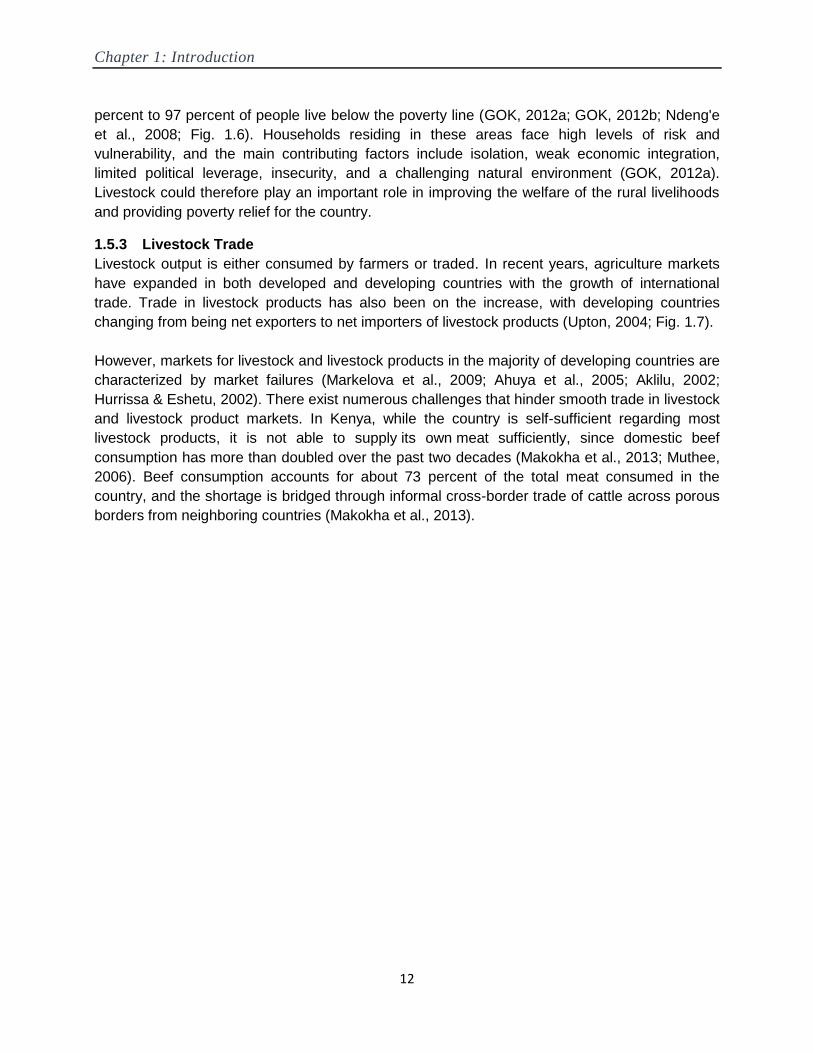
percent to 97 percent of people live below the poverty line (GOK, 2012a; GOK, 2012b; Ndeng'e
et al., 2008; Fig. 1.6). Households residing in these areas face high levels of risk and
vulnerability, and the main contributing factors include isolation, weak economic integration,
limited political leverage, insecurity, and a challenging natural environment (GOK, 2012a).
Livestock could therefore play an important role in improving the welfare of the rural livelihoods
and providing poverty relief for the country.
1.5.3 Livestock Trade
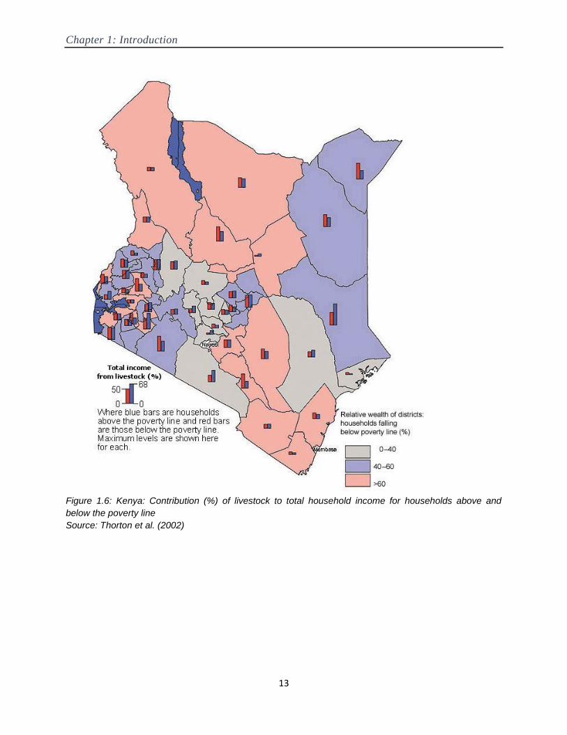
Livestock output is either consumed by farmers or traded. In recent years, agriculture markets
have expanded in both developed and developing countries with the growth of international
trade. Trade in livestock products has also been on the increase, with developing countries
changing from being net exporters to net importers of livestock products (Upton, 2004; Fig. 1.7).
However, markets for livestock and livestock products in the majority of developing countries are
characterized by market failures (Markelova et al., 2009; Ahuya et al., 2005; Aklilu, 2002;
Hurrissa & Eshetu, 2002). There exist numerous challenges that hinder smooth trade in livestock
and livestock product markets. In Kenya, while the country is self-sufficient regarding most
livestock products, it is not able to supply its own meat sufficiently, since domestic beef
consumption has more than doubled over the past two decades (Makokha et al., 2013; Muthee,
2006). Beef consumption accounts for about 73 percent of the total meat consumed in the
country, and the shortage is bridged through informal cross-border trade of cattle across porous
borders from neighboring countries (Makokha et al., 2013).
Chapter 1: Introduction
13
Figure 1.6: Kenya: Contribution (%) of livestock to total household income for households above and
below the poverty line
Source: Thorton et al. (2002)
Chapter 1: Introduction
14
Figure 1.7: Cattle meat trade in least developed countries
Source: FAOSTAT Database
0
10000
20000
30000
40000
50000
60000
19
61
19
63
19
65
19
67
19
69
19
71
19
73
19
75
19
77
19
79
19
81
19
83
19
85
19
87
19
89
19
91
19
93
19
95
19
97
19
99
20
01
20
03
20
05
20
07
20
09
20
11
Qu
anti
ty T
rad
ed
(To
nn
es)
Cattle Meat Trade in Least Developed Countries
Import Quantity
Export Quantity
Chapter 1: Introduction
15
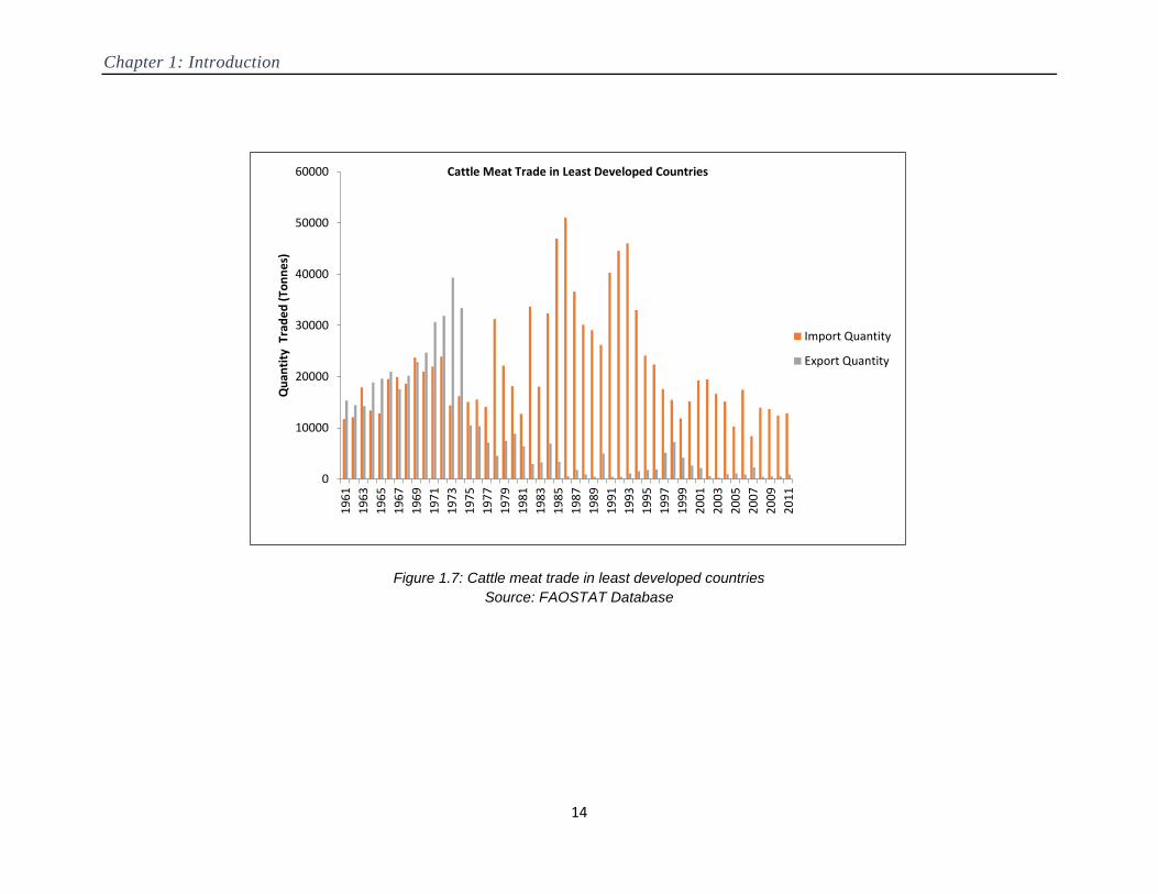
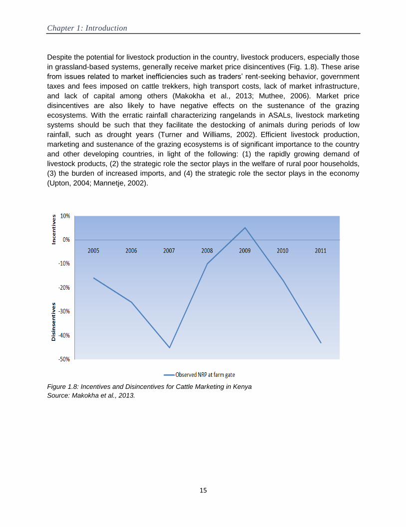
Despite the potential for livestock production in the country, livestock producers, especially those
in grassland-based systems, generally receive market price disincentives (Fig. 1.8). These arise
from issues related to market inefficiencies such as traders‘ rent-seeking behavior, government
taxes and fees imposed on cattle trekkers, high transport costs, lack of market infrastructure,
and lack of capital among others (Makokha et al., 2013; Muthee, 2006). Market price
disincentives are also likely to have negative effects on the sustenance of the grazing
ecosystems. With the erratic rainfall characterizing rangelands in ASALs, livestock marketing
systems should be such that they facilitate the destocking of animals during periods of low
rainfall, such as drought years (Turner and Williams, 2002). Efficient livestock production,
marketing and sustenance of the grazing ecosystems is of significant importance to the country
and other developing countries, in light of the following: (1) the rapidly growing demand of
livestock products, (2) the strategic role the sector plays in the welfare of rural poor households,
(3) the burden of increased imports, and (4) the strategic role the sector plays in the economy
(Upton, 2004; Mannetje, 2002).
Figure 1.8: Incentives and Disincentives for Cattle Marketing in Kenya
Source: Makokha et al., 2013.

Chapter 1: Introduction
16
Chapter Two
2 Land Use/Land Cover Changes on Global Livestock
Grazing Ecosystems
: A review of the natural rangelands systems dynamics
2.1 Introduction
Natural rangeland systems are mainly used as native grazing pastures and are defined here as
―ecosystems which carry a vegetation consisting of native and/or naturalized species of grasses
and dicotyledonous herbs, trees and shrubs, used for grazing or browsing by wild and domestic
animals, on which management is restricted to grazing, burning, and control of woody plants‖
(Mannetje, 2002). In addition to providing 50% of the world‘s livestock, the ecosystems
encompass a significant portion of the world‘s biodiversity and culturally diverse habitats and are
also of great ecological significance (Davies et al., 2015; Kreutzmann et al., 2011; Mannetje,
2002). The ecosystems are also vast and estimated to occupy about 50% of the world‘s total
land area (Kiage, 2013; Friedel et al., 2000; Mathews, 1986; Davies et al., 2015; Mannetje,
2002).
Despite providing crucial ecosystem services, rangeland areas are being degraded, particularly
in the arid and semi-arid environments of Africa and Asia (Steinfeld et al., 2006b; UNEP, 2007;
Neely et al., 2009). Understanding rangeland dynamics and the paths of degradation is critical in
the design of sustainable rangeland use. Numerous factors, as discussed later in the chapter,
have been identified to contribute to the degradation of rangeland areas. A critical review of the
drivers supports the current emerging views acknowledging the presence and interaction of both
equilibrium and non-equilibrium factors in explaining the dynamics of the productivity of
rangelands (Vetter, 2005; Domptail, 2011). The equilibrium model theory, which is mostly used
in studying rangeland dynamics, centers on density-dependent factors such as stocking rates
and the feedback of grazing pressure on vegetation composition, cover, and productivity. This
theory stresses the importance of carrying capacity of rangelands resulting in interventions of
maximum stock numbers to be allowed in an attempt to halt degradation and sustain rangelands
(Vetter, 2005). In contrast, the disequilibrium theory views the ecology of rangelands as being
best conceptualized in terms of non-equilibrium dynamics.
Chapter 2: Land use/land cover changes on global livestock grazing ecosystems
17
According to the theory, rangeland productivity is constrained by density-independent factors
such as climatic variability and other external shocks to the system rather than by density-
dependent factors (Boyd et al., 1999; Ramankutty et al., 2006). The disequilibrium theory implies
that stocking strategies are less damaging to rangeland ecosystems and have negligible
ecological effects (Kiage, 2013). However, an analysis of the literature on drivers of rangeland
degradation illustrates that both density-dependent factors and density-independent factors,
such as climate and anthropogenic factors, are responsible for rangeland degradation. This
paper unfolds the existence of density-independent factors on native rangelands, their
emergence, how they modify the ecosystems, and their possible interactions with density-
dependent factors.
The literature review reveals that a large share of the identified drivers of rangeland degradation,
as it is the case with other terrestrial ecosystems in the world, relates to land use/land cover
changes. Significant environments in the world are experiencing land use/land cover changes, a
density-independent factor, which in most cases is often associated with loss of natural
vegetation, biodiversity loss, long-term productivity capacity losses, and ecological services
losses among others (Foley et al., 2005; Kiage et al., 2007; Maitima et al., 2009). In addition,
land use/land cover changes in rangelands are likely to interact with density dependent factors,
resulting in either positive or negative consequences for the environment (Fig 2.1). For instance,
as observed in extensive rangeland systems, land use/land cover changes resulting in the loss
of pasture areas are likely to lead to restricted livestock mobility and access to pastoral
resources which are necessary for sustainable rangeland use (Homewood et al., 2012; Flintan,
2011; Eva et al., 2006; Campbell et al., 2003; Campbell et al., 2005; Butt, 2010).
This chapter reviews the evidence on land use/land cover changes in global native rangelands
over the last six decades. It first shows the trend of land use/land cover changes in rangelands
and demonstrates that the processes are global. The analysis over an extended period of time
offers more support of the trends compared to analyses over specific short-term periods, such
as changes over a period of five years (Nickerson et al., 2011). Second, the dynamics of the
land use/land cover changes are explored, indicating sources and destinations of rangelands
losses/gains. Third, the chapter makes an evaluation to determine the related effects of native
rangeland dynamics on the health of the ecosystems. This paper presents a balanced picture by
demonstrating that not all losses of native rangelands are pessimistic and neither are all gains
associated with better-managed systems.
2.2 Resource use/cover changes on native grazing lands – Area
Large environments of the world have experienced significant land cover changes.
Comprehensive studies carried out all over the world identify significant landscape changes on
rangelands associated with human activities. Land use/land cover changes are either associated
with land cover conversions, which in our case would involve the complete replacement of
grazing vegetation by another land cover type, or land cover modifications whereby the overall
classification of the land cover is maintained but the character of the land cover is affected
(Lambin et al., 2001; Lambin et al., 2003; Maitima et al., 2009; Reid et al., 2004). Figure 2.1
shows the possible transformations of grazing lands.
Chapter 2: Land use/land cover changes on global livestock grazing ecosystems
18
Source: Author’s conceptualization.
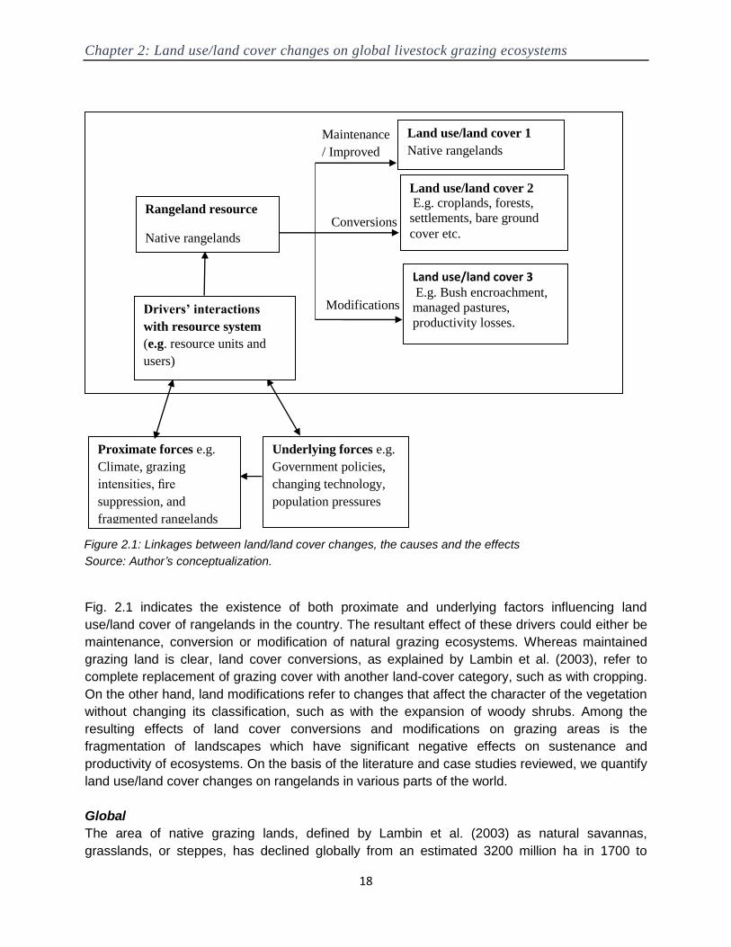
Fig. 2.1 indicates the existence of both proximate and underlying factors influencing land
use/land cover of rangelands in the country. The resultant effect of these drivers could either be
maintenance, conversion or modification of natural grazing ecosystems. Whereas maintained
grazing land is clear, land cover conversions, as explained by Lambin et al. (2003), refer to
complete replacement of grazing cover with another land-cover category, such as with cropping.
On the other hand, land modifications refer to changes that affect the character of the vegetation
without changing its classification, such as with the expansion of woody shrubs. Among the
resulting effects of land cover conversions and modifications on grazing areas is the
fragmentation of landscapes which have significant negative effects on sustenance and
productivity of ecosystems. On the basis of the literature and case studies reviewed, we quantify
land use/land cover changes on rangelands in various parts of the world.
Global
The area of native grazing lands, defined by Lambin et al. (2003) as natural savannas,
grasslands, or steppes, has declined globally from an estimated 3200 million ha in 1700 to
Figure 2.1: Linkages between land/land cover changes, the causes and the effects
Proximate forces e.g.
Climate, grazing
intensities, fire
suppression, and
fragmented rangelands
Underlying forces e.g.
Government policies,
changing technology,
population pressures
Maintenance
/ Improved
Conversions
Modifications
Land use/land cover 1
Native rangelands
Rangeland resource
Native rangelands
Land use/land cover 3 E.g. Bush encroachment,
managed pastures,
productivity losses.
Drivers’ interactions
with resource system
(e.g. resource units and
users)
Land use/land cover 2
E.g. croplands, forests,
settlements, bare ground
cover etc.

Chapter 2: Land use/land cover changes on global livestock grazing ecosystems
19
1800–2700 million ha in 1990 (Lambin et al., 2003). Recent global estimates of grazing lands,
however, indicate that the ecosystems have experienced less dramatic changes. The overall
estimates of global land cover from FAO‘s regional data indicate relatively stable grazing lands,
defined as ―land used permanently for herbaceous forage crops, either cultivated or naturally
growing‖ (FAOSTAT Database). The grazing lands are estimated to have slightly declined by
0.89% globally between the periods 1961 and 2011 (FAOSTAT Database). The estimates by
FAO, however, do not differentiate between modified/improved pastures and extensive native
grazing lands. This lack of differentiation could explain the relative stability of the grazing areas.
Even so, the estimates do indicate varying grazing lands from one region to another.
Africa
In Africa, grazing lands have declined considerably from 84.02% to 77.92% of agricultural
area/land area between 1961 and 2011 (FAOSTAT Database). The decline is relatively large in
Eastern Africa and Western Africa, with declines of 8.88% and 8.59%, respectively (FAO 2013).
The grazing ecosystems in the continent are dominated by natural pastures mainly composed of
grasslands interrupted by woody vegetation (Kiage, 2013). Therefore, the trend described above
can be taken to represent the dynamics of the native grazing ecosystems found on the
continent.
Similar observations of declining grazing lands are made by several other studies on land
use/cover changes in the region. Brink & Eva (2009) estimated the land cover changes for Sub-
Saharan Africa between 1975 and 2000. The authors estimated that land cover classified as
natural non-forest vegetation, comprising of natural vegetation such as grassland, bush land,
shrub lands, and wooded grassland, diminished by 4.72%. Based on White‘s (1983) vegetation
categories of Africa, the Sudanian, Sahel, Somalia-Masai, and Guineo-Congolian regions had
the largest significant declines of 35.9%, 29.2%, 18.9%, and 8.1%, respectively (Eva et al.,
2006). In Eastern Africa, land use and land cover changes in Kagera Basin, spanning across
Burundi, Rwanda, Uganda, and Tanzania between 1901 and 2010, indicate a decline in
savannas by 15.4% between 1901 and 2010 (Wasige et al., 2013). A similar study in the area
between 1984‒2011 indicated a decrease in Woodland savanna by 12.4% (Berakhi et al.,
2014).
Comparable trends of declining grazing lands are observed in country case studies over the vast
West African region. In Burkina Faso, between the years 1975 and 2000, savannas declined
from 59.8% to 51.6% of the land area, while in Niger, steppes and savannas mainly used as
extensive grazing lands decreased by 3.4% and 16.2%, respectively (Tappan and Cushing,
2013). In Togo, the country's savannas and woodlands declined by 10%, in Mauritania by 30%,
in Benin by 10.4%, and in Guinea by 1.9% (Tappan and Cushing, 2013). In Senegal, the
country‘s diverse savannas declined by 4.1% between 1965 and 2000 (Tappan et al., 2004). In
South Africa, changes in land use/land cover between 1961 and 2006 indicated relatively stable
conditions throughout the period (Niedertscheider et al., 2012). Within the period of 1961 to
1988, grasslands declined by 20,000 sq. km., but from 1988 to 2006, the ecosystems increased
back to 1961 values of about 270,000 sq. km. These observations are similar to the findings by
Brink and Eva (2009) and Eva et al. (2006), who found no significant land cover changes in the
Karoo-Namib and Kalahari-Highveld regions between the years 1975 and 2000.
Chapter 2: Land use/land cover changes on global livestock grazing ecosystems
20
Asia
FAO‘s regional data on land cover indicates that grazing lands in Asia increased by 7.31%
between 1961 and 2011 (FAOSTAT Database). Much more pronounced was the increase in
Western Asia (7.32%), followed by Eastern Asia (2.32%) with an increase of 6.33% in China
(FAOSTAT Database). Values of grazing areas, however, declined in Southern Asia and South-
Eastern Asia by 5.82% and 5.73%, respectively, and in Central Asia by 0.65% (FAOSTAT
Database). In Central Asia, land use/land cover changes from 1990–2009 indicate that natural
vegetation comprising woody savanna or shrub canopy cover, herbaceous cover, and other
natural vegetation types, increased by 10.67% of the land area (Chen et al., 2013). The change
represented a 16.69% increase in natural vegetation cover from 1990 to 2000 following the
conversion of abandoned farmland to natural vegetation such as grassland and shrubland (Chen
et al., 2013). However, from 2000 to 2009, the area of natural vegetation declined by 5.16%
following the reclamation of abandoned farmland (Chen et al., 2013).
Extensive research on land-use changes in montane mainland Southeast Asia in Thailand,
Yunnan (China), Vietnam, Cambodia, and Laos is available for the period of 1950-2000. The
results indicate that the increase in grazing lands, defined as grass, bamboo, and bushes, was
greatest in Tan Minh, northern Vietnam, from 27% to 67% (1952-1995). Grazing areas were also
observed to be on the increase in Mengsong, Southern Yunnan; in Ban Khun, Northern
Thailand; and in Ang Nhai, Laos (Fox and Vogler, 2005). On the other hand, significant declines
in grazing areas were observed in Baka, Southern Yunnan (25%) and Menglong, Southern
Yunnan (12%) in the period of 1965-1992. Additional areas with declining grazing areas included
Mae Tho, Northern Thailand and Ban Lung, Northeastern Cambodia (Fox and Vogler, 2005).
In Eastern Asia, land use/land cover changes in China indicate significant increases in grassland
from 1988-1995 (Yang and Li, 2000). Over this period, gains of 18.5% in grasslands in the entire
nation emerged from losses of cultivated land across provinces in the country. However, some
areas in the country observed losses in grazing lands as in the case of Xishuangbanna,
Southwest China (Hu et al., 2008; Fox and Vogler, 2005). In Xishuangbanna, Southwest China,
swidden fields, defined as lands that have the ecological functions of grassland/rangeland,
declined from 13.14% to 0.46% between 1988 and 2006 (Hu et al., 2008). On the other hand,
shrubland declined from 17.29% in 1988 to 16.05% in 2006 (Hu et al., 2008). In addition, land-
use changes in China between the years 1995-2000 feature a 134,4861 square hectometer
(hm2) decline in grasslands (Liu et al., 2003).
America
FAO‘s regional data on land cover in America indicates slight decreases in the area of grazing
land of about 1.46% for the period 1961-2011 (FAOSTAT Database). The changes, however,
vary across regions; for example, there were significant declines in grazing areas in South
America (8.22%) and among the Caribbean countries (7.31%; FAOSTAT Database). Grazing
areas also declined in Central America (3.41%), but in Northern America, there were notable
exceptions to the declining trend, with a slight increase (1.03%) in the grazing areas (FAOSTAT
Database).
During the earlier periods, changes in the landscape in Latin America indicate that
approximately 83.21% of the grassland was lost between 1850 and 1985 from 310*106 ha to

Chapter 2: Land use/land cover changes on global livestock grazing ecosystems
21
52*106 (Houghton et al., 1991). In the South American Temperate grasslands, changes in land
use and land cover in the periods of 1985–1989 and 2002–2004 indicate that grasslands,
comprising prairie and grass steppes, decreased from 67.4% (151,320 km²) to 61.4% (137,817
km²), a relative change of -8.9% (Baldi and Paruelo, 2008). Whereas in the Patagonian
landscapes in South America, the landscape structure between 1940 and 1970 indicates a
dominant decrease in shrublands by 40.9% and 20.4% in the coastal (LTC) and inland (LTI)
areas, respectively (Kitzberger and Veblen 1999). Grasslands were observed to have a relatively
smaller transition; they declined by 2.3% and 18.5% in coastal and inland areas, respectively
(Kitzberger and Veblen 1999). On the other hand, extensive research on land-use changes in
non-Amazonian South America estimating the difference between the present (2009-2012) and
potential vegetation extent indicated a decline in savannas and grasslands by 52% and 70%,
respectively (Salazar et al., 2015).
In North America, land cover changes by the North American Land Change Monitoring System
(NALCMS) from 2005-2010 indicate that grasslands in Mexico gained a net of 172km2 (Land
cover monitoring | Biodiversidad Mexicana, n.d.). A similar study in the Yucatan Peninsula,
Mexico, indicated similar trends in increasing grazing areas with an increase in tropical
grasslands by 8% between the years of 2000 and 2005 (Mascorro et al., 2014). In the U.S.,
land-use change indicates a decline in total grazing lands by about 26% (274 million acres) from
1945 to 2007. In the same period, grassland pasture and range declined by almost 7% (45
million acres). However, recently (2002-07), grassland pasture and range increased by almost
5% (27 million acres), offsetting the 26 million acre decline in cropland pasture. On the other
hand, grazed forestland was observed to be on a continuous decline, with estimates of about
218 million acres lost (63%) during 1945- 2007, and 7 million acres lost during 2002-07
(Nickerson et al., 2011).
Europe
According to FAO‘s regional dataset, grazing areas in Europe declined by about 12.17%
between 1961 and 2011 (FAOSTAT Database). However, from 1961-1991, grasslands
increased by 2.59% from 50.01% to 52.6% (FAOSTAT Database). A significant decline from
52.6% in 1991 to 37.63% in 2001 is then observed, and thereafter, the grazing areas are
maintained at relatively the same level (FAOSTAT Database). The significant decline is mainly
driven by a drastic decline in Eastern Europe over the same period and can be associated with
the drop of the Union of Soviet Socialist Republics (USSR) data from the dataset.
An extensive study on land cover/land changes for the EU27 plus Switzerland using Historic
Land Dynamics Assessment (HILDA) version 2.0 is used to assess historic net changes in
grasslands in Europe. Grasslands in the study are defined to include natural grasslands,
wetlands, pastures, and mediterranean shrub vegetation. Between 1900 and 2010, the HILDA
net change indicated that grasslands had decreased by 16.11%, while between 1950 and 2010,
grasslands are observed to have declined by 7.02% (Fuchs et al., 2013; Fuchs et al., 2015a;
Fuchs et al., 2015b). However, in the most recent periods, 1990-2010 and 2000-2010,
grasslands increased by 4.49% and 3.04%, respectively (Fuchs et al., 2013; Fuchs et al., 2015a;
Fuchs et al., 2015b).
Chapter 2: Land use/land cover changes on global livestock grazing ecosystems
22
Local studies on land cover change over similar recent periods in the area indicate similar
trends. In the Netherlands, land cover changes in the years 1986–2000 indicate that shrubs
and/or herbaceous vegetation increased from 19.1 km2 to 92.3 km2 (Feranec et al., 2007). On
the other hand, in the Slovak Republic, land cover changes for the period 1970–1990 indicates
that shrubs and/or herbaceous vegetation increased from 96.6 km2 to 922.4 km2 (Feranec et al.,
2007).
Australia
FAO estimates of grazing land in Australia & New Zealand indicate decreases of about 4.56% in
the period of 1961-2011 (FAOSTAT Database). Similar observations are made by a study
conducted to track the land use change in Australia from 1992–93 and 2005–06 (Lesslie et al.,
2011). Observations indicate a steady decline in the total grazing areas from 4,551,100 sq. km.
from 1992-93 to 4,287,600 sq. km from 2005-06 (6%; Lesslie et al., 2011; Mewett et al., 2013).
The decline includes a decrease of 149,600 sq. km. (3.37%) in the most recent period (2000-01
to 2005-06; Lesslie et al., 2011). In the period of 2005-2006, grazing natural vegetation occurred
on 46.30% of the land area (3,558,785 sq.km) and grazing modified pastures occurred on 9.37%
of the land area (720,182 sq.km), while irrigated pastures occupied 0.13% (10,011 sq.km) of the
land area (Lesslie et al., 2011). This indicates that native grazing lands are likely to have had a
higher share of decline.
Recent studies provide more evidence on the declining grazing lands. Between the period
1992–93 to 2009–10, agricultural land uses, comprising grazing and cropped areas declined by
11% (Mewett et al., 2013). Other studies estimate the decline to have been by 8% over the
same period (Lesslie et al., 2011). During the same period, crop areas (excluding grazing areas
and pasture crops) increased by 50%, up by 40% between the period of 1992–93 and 2005–06
(Lesslie et al., 2011). The above implies that the decline in the agricultural area between the
period of 1992–93 and 2009–10 was mainly from grazing areas.

Chapter 2: Land use/land cover changes on global livestock grazing ecosystems
23
Table 2.1: Summary of Land Use/Land Cover changes in global grasslands
Region Ecosystem Trend over time Net Gains From Net Losses To References
WORLD Permanent meadows and pastures-
% of agricultural area /land area 1961 2011 FAOSTAT Database
69.27% 68.38%
Natural savannas, grasslands or
steppes (million ha)
1700 1990 Lambin et al. (2001)
3200 1800–2700
AFRICA Permanent meadows and pastures 1961 2011 FAOSTAT Database
84.02 77.92
Sub-Saharan Africa Natural non-forest vegetation (ha) 1975 2000 - Agriculture
- Barren
Brink & Eva (2009) ;
Eva et al. (2006) 1,247,980 1,189,085
Kagera basin
Savannas (% of land use/cover in
the basin) 1901 2010 - Farmland Wasige et al. (2013)
35% 19.6%
Woodland savanna (% of land
use/cover in the basin)
1984 2011 - Wetlands
- Agricultural land
- Forests
- Urban land and Water
bodies
Berakhi et al. (2014)
43.7% 31.3%
Ethiopia Grasslands - Invasive bushes Admasu (2008)
South Africa Grasslands (sq. km of national land
use/ land cover) 1961 1988 2006 Niedertscheider et al.
(2012) 270,000 250,000 270,000
Namibia Grasslands - Invasive bushes Mlunga &
Gschwender (2015)
Senegal
Savanna -% National land use and
land cover trends 1965 2000 - Agricultural land
- Steppes
- Bare ground cover
Tappan et al. (2004)
Tappan & Cushing
(2013) 73.7% 69.6%
Savannas and woodlands
(% National land use and land
cover trends)
1975 2000 - Cropping lands
- Wild lands
- Protected areas
- Bare surfaces
- Sandy surfaces
- Steppe vegetation
Tappan & Cushing
(2013)
Burkina Faso 59.8% 51.6%
Togo 78.1% 68.1%
Guinea 75.9% 74%
Benin 80% 69.6%
Niger Savannas decreased by 16.2%
Mauritania Savannas decreased by 30%
Permanent meadows and pastures 1961 2011 FAOSTAT Database
ASIA 58.8 66.11
Central Asia Natural vegetation area (100,000
sq.km) 1990 2000 2009 Abandoned farmland Chen et al. (2013)
28.30 33.03 31.32
Southwest China Swidden field (% of total land area) 1988 2006 - Crop lands (rubber
plantations)
Hu et al. (2008)
13.14% 0.46%

Chapter 2: Land use/land cover changes on global livestock grazing ecosystems
24
Region Ecosystem Trend over time Gains From Losses To References
Period 1950- 2000 Fox and Vogler
(2005) Tan Minh
Grass, bamboo, bushes (% of land
use/land cover)
27% 67% - closed and open
canopy forests
Ban Lung 9% 3% - agriculture
Mae Tho 6% 4% - agriculture
Baka
32 7% - closed and open
canopy forests
Mengsong 35 43% - closed canopy cover
Menglong 26 14% - agriculture
Ban Khun 10% 18% - closed-canopy cover
China 1988 1995 - Cropland (e.g.
conservation efforts)
- abandonment of poor
quality cultivated land
Yang and Li (2000).
Grasslands(% gains from total
converted cultivated land)
18.5% gains
China Grassland (square hectometer) 1995 to 2000 arable land Liu et al. (2003).
Decline in area by 1,344,861
Permanent meadows and pastures 1961 2011 FAOSTAT Database
AMERICA 68.65 67.19
Latin America Grassland (exclusive of pastures, in
106 ha)
1850 1985 - crops
- pasture areas
Houghton et al.
(1991) 310 52
South American
Temperate
Grasslands
Grasslands- prairie and grass
steppe (% of land area)
1985-1989 2002–2004 - agricultural expansion
- afforestation
Baldi and Paruelo
(2008)
67.4% 61.4%
Patagonian
landscapes in South
America
1940 1970 - forests Kitzberger and
Veblen (1999) Grasslands (Class area (%)) 7.3% (LTC) 5% (LTC) - shrublands
28.3% (LTI) 9.8% (LTI)
Non-Amazonian
South America
Grasslands area (km2) Potential
historic area
Present area
(2009-2012)
- crop and pastures
- forests
777,571 236,240 Salazar et al. (2015)
Mexico 2005 2010 - shrublands
- cropland
- forest covers
- wetlands
- barren land
- urban and built-up
- water
Land cover
monitoring |
Biodiversidad
Mexicana, (n.d.)
Grasslands 359 531
Yucatan Peninsula,
Mexico
2000 2005 - harvesting
- hurricanes
Mascorro et al. (2014)
Tropical
Grassland
Tropical grasslands increased by
8%
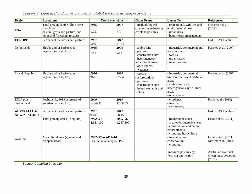
Chapter 2: Land use/land cover changes on global livestock grazing ecosystems
25
Region Ecosystem Trend over time Gains From Losses To References
USA
Total grazing land Million acres
(cropland
pasture, grassland pasture, and
range and forestland grazed).
1945 2007 - methodological
changes in estimating
cropland pastures
- recreational, wildlife, and
environmental uses
- urban uses
- better forest management
Nickerson et al.
(2011) 1,051 777
EUROPE Permanent meadows and pastures 1961 2011 FAOSTAT Database
50.01 37.84
Netherlands Shrubs and/or herbaceous
vegetation (in sq. km) 1986 2000 - arable land
- pastures
- construction sites
- heterogeneous
agricultural areas
- open spaces
- wetlands
- industrial, commercial and
transport units
- forests
- urban fabric
- inland waters
Feranec et al. (2007)
19.1 92.3
Slovak Republic Shrubs and/or herbaceous
vegetation (in sq. km) 1970 1990 - forests
(deforestation)
- pastures
- construction sites
- inland wetlands and
waters
- industrial, commercial
transport units and artificial
areas
- arable land and
heterogeneous agricultural
areas
- open spaces
Feranec et al. (2007)
96.6 922.4
EU27 plus
Switzerland
Fuchs et al., 2013 estimates of
grasslands (in sq. km) 1900 2010 - croplands
- forests
- settlements
Fuchs et al. (2013)
1484992 1245803
AUSTRALIA &
NEW ZEALAND
Permanent meadows and pastures 1961 2011 FAOSTAT Database
93.01 88.45
Australia
Total grazing areas (in sq. km) 1992–93 2005–06 - modified pastures
- area under intensive uses
- conservation and natural
environments
- cropping/ horticulture
Lesslie et al. (2011)
4,551,100 4,287,600
Agricultural area (grazing and
cropped areas) 1992–93 to 2009–10 - formal nature
conservation
- cropping
Lesslie et al. (2011)
Mewett et al. (2013) Decline in area by 8-11%
improved pastures by
fertiliser application
Australian National
Greenhouse Accounts
(2013)
Source: Compiled by author
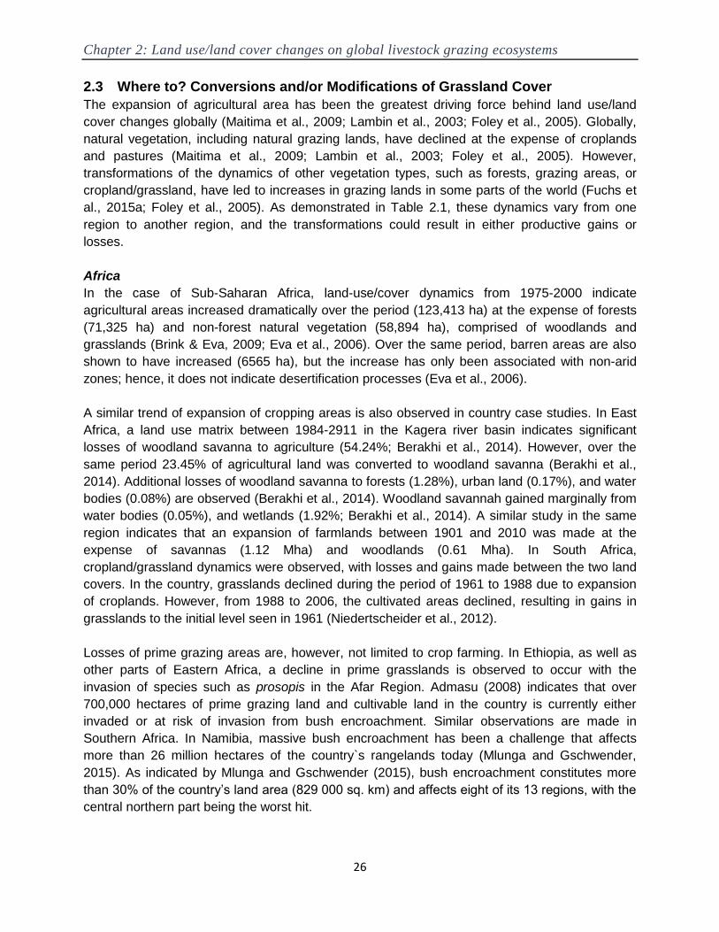
Chapter 2: Land use/land cover changes on global livestock grazing ecosystems
26
2.3 Where to? Conversions and/or Modifications of Grassland Cover
The expansion of agricultural area has been the greatest driving force behind land use/land
cover changes globally (Maitima et al., 2009; Lambin et al., 2003; Foley et al., 2005). Globally,
natural vegetation, including natural grazing lands, have declined at the expense of croplands
and pastures (Maitima et al., 2009; Lambin et al., 2003; Foley et al., 2005). However,
transformations of the dynamics of other vegetation types, such as forests, grazing areas, or
cropland/grassland, have led to increases in grazing lands in some parts of the world (Fuchs et
al., 2015a; Foley et al., 2005). As demonstrated in Table 2.1, these dynamics vary from one
region to another region, and the transformations could result in either productive gains or
losses.
Africa
In the case of Sub-Saharan Africa, land-use/cover dynamics from 1975-2000 indicate
agricultural areas increased dramatically over the period (123,413 ha) at the expense of forests
(71,325 ha) and non-forest natural vegetation (58,894 ha), comprised of woodlands and
grasslands (Brink & Eva, 2009; Eva et al., 2006). Over the same period, barren areas are also
shown to have increased (6565 ha), but the increase has only been associated with non-arid
zones; hence, it does not indicate desertification processes (Eva et al., 2006).
A similar trend of expansion of cropping areas is also observed in country case studies. In East
Africa, a land use matrix between 1984-2911 in the Kagera river basin indicates significant
losses of woodland savanna to agriculture (54.24%; Berakhi et al., 2014). However, over the
same period 23.45% of agricultural land was converted to woodland savanna (Berakhi et al.,
2014). Additional losses of woodland savanna to forests (1.28%), urban land (0.17%), and water
bodies (0.08%) are observed (Berakhi et al., 2014). Woodland savannah gained marginally from
water bodies (0.05%), and wetlands (1.92%; Berakhi et al., 2014). A similar study in the same
region indicates that an expansion of farmlands between 1901 and 2010 was made at the
expense of savannas (1.12 Mha) and woodlands (0.61 Mha). In South Africa,
cropland/grassland dynamics were observed, with losses and gains made between the two land
covers. In the country, grasslands declined during the period of 1961 to 1988 due to expansion
of croplands. However, from 1988 to 2006, the cultivated areas declined, resulting in gains in
grasslands to the initial level seen in 1961 (Niedertscheider et al., 2012).
Losses of prime grazing areas are, however, not limited to crop farming. In Ethiopia, as well as
other parts of Eastern Africa, a decline in prime grasslands is observed to occur with the
invasion of species such as prosopis in the Afar Region. Admasu (2008) indicates that over
700,000 hectares of prime grazing land and cultivable land in the country is currently either
invaded or at risk of invasion from bush encroachment. Similar observations are made in
Southern Africa. In Namibia, massive bush encroachment has been a challenge that affects
more than 26 million hectares of the country`s rangelands today (Mlunga and Gschwender,
2015). As indicated by Mlunga and Gschwender (2015), bush encroachment constitutes more
than 30% of the country‘s land area (829 000 sq. km) and affects eight of its 13 regions, with the
central northern part being the worst hit.

Chapter 2: Land use/land cover changes on global livestock grazing ecosystems
27
Transformations of the native grazing lands in Western Africa portray a similar trend to the rest
of the continent. In West Africa, expansion of agricultural land and climatic factors are cited to be
the main driving force towards declining grazing areas over the period 1975 to 2000 (Tappan
and Matthew Cushing, 2013). Despite savannas and woodlands being the dominant land
use/land cover in most parts of the region, expansion of agricultural land overrides these
ecosystems (Tappan and Matthew Cushing, 2013). In Benin, the increase in agricultural areas is
observed to have been at the expense of savannas and woodlands and other wild lands and
protected areas. Similar observations are made in Burkina Faso, where expansion of cropland
has led to the shrinking of the natural savannas with the increasing population pressures
(Tappan and Matthew Cushing, 2013). Comparable to other regions, expansion of cropping
lands in Guinea is most commonly explained by declining savannas and woodland areas, with
modest losses in forest areas (Tappan and Matthew Cushing, 2013). In Ghana, Senegal, and
Togo, expansion of agricultural land was observed to fragment savannas and woodlands. In
Senegal, harsh climatic conditions have led to the loss of savanna to steppes (4.9%) and
increased bare cover (20.1%), mainly in the pastoral regions (Tappan and Matthew Cushing,
2013). However, in some parts of the country, abandoned agricultural land (11.2%) due to crisis
periods in the agricultural economy gave rise to long-term fallows classified as shrub and tree
savanna vegetation types (Tappan and Matthew Cushing, 2013). A similar study in Senegal,
from 1965-2000, indicates encroachment of agricultural land on the country‘s diverse savannas
(Tappan et al., 2004). In addition, the diverse savannas declined by 0.4% and 1% with the
expansion of steppes cover and bare ground cover (degraded areas), respectively. Similarly, in
Niger, steppe and savanna vegetation are indicated to have declined mainly due to the
expansion of agricultural land but also partly due to drought. Sandy surfaces are observed to
have expanded (37%) in the steppes of the Mauritania's Sahelian and Saharo-Sahelian regions
due to drought and encroachment of steppe vegetation (Tappan and Matthew Cushing, 2013).
Although the agricultural area in Mauritania increased – rain fed cropping by about 700 sq. km
and irrigated by about 300 sq. km – its effect on the herbaceous vegetation was modest.
Asia
In Central Asia, the increase in natural vegetation by 4.73*105sq. km between the years 1990
and 2000 approximated the decrease in farmland by 4.89 *105sq. km over the same period
(Chen et al., 2013). As indicated by Chen et al. (2013), the dynamics reflect the conversion of
abandoned farmland to natural vegetation such as grassland and shrubland. However, between
the period of 2000 and 2009, farmland increased by 1.62 *105 sq. km., whereas natural
vegetation declined by a similar amount (1.71 *105sq. km), reflecting reclamation of some of the
abandoned farmland (Chen et al., 2013). In Southwest China, losses in swidden fields, which
have a biome equivalent to that of grass/rangelands, are attributed to shifts to large-scale rubber
plantations, resulting in significant losses in ecosystem services (Hu et al., 2008).
In Montane Mainland Southeast Asia, with the growing population pressures, the presence of
government interventions to slow down transformations of tree cover or encouraging agriculture
played a big role in land use/land cover changes. In areas such as Baka, Southern Yunnan, the
establishment of a nature reserve by the national government resulted in gains in closed and
open-canopy forest cover, with losses in other vegetation covers such as grass, bamboo, and
bushes (Fox and Vogler, 2005). However, in the absence of such interventions, as was the case
in Mengsong, Southern Yunnan, tree covers were cleared between the years 1949 and 1992, in

Chapter 2: Land use/land cover changes on global livestock grazing ecosystems
28
efforts towards self-sufficiency in food. Where more land was cleared than needed, gains in
grass, bamboo, and bush categories were observed (Fox and Vogler, 2005).
Similarly, in China, gains in grasslands within the period of 1988-1995 were mainly from losses
in cultivated areas. The increase in demand for fruits and aquatic products in response to high
incomes led to the loss of cultivated land to horticulture and fish ponds. Where the destination of
such conversions was not land to horticulture and fish ponds, the land was converted to other
uses such as grasslands (Yang and Li, 2000). In addition, cropland-grassland conversions have
been as a result of abandonment of poor quality land especially in the arid and semi-arid areas.
However, reclamation of such crop lands has been on the increase with the increasing
population pressures and demand for food (Yang and Li, 2000). Cropland-grassland
conversions in the country have also been as a result of some land-conservation projects efforts
conducted in the arid and semi-arid areas of the country, such as the Three-north Forest
Protection Belt Program (Yang and Li, 2000). The reclamation of arable land from grasslands is
further demonstrated by land-use/cover dynamics from 1995-2000 (Liu et al., 2003). Over this
period, the net losses of grassland were mainly to arable land.
Europe
Land cover/land use changes in grasslands in Europe are demonstrated to be significantly
determined by settlements (urbanization), afforestation/reforestation (and, in some instances,
deforestation), and cropland/grassland dynamics (Fuchs et al., 2015a). Land use/land cover
changes in Europe (EU27 plus Switzerland) between 1900 and 2010 demonstrate that, of all
gains in grasslands (30.4% of the entire area covered), 20.4% were from cropland, 7.1% are a
result of deforestation, and 1.6% are from settlements (Fuchs et al., 2015a). On the other hand,
of all the grassland losses (37% of the entire area covered), 5.5% were to settlements, 20.8%
were to croplands, and 9.4% were to forests (Fuchs et al., 2015a). Similar trends are observed
in local case studies in the region.
In the Netherlands, the effort to fulfill the country‘s biodiversity goals has resulted in the
conversion of agricultural land to shrub and/or herbaceous vegetation and other natural and/or
semi-natural land such as forests and inland wetlands. In the period of 1986–2000, net gains of
37.3 sq. km of arable land and 13.9 sq. km of pastures to shrub and/or herbaceous vegetation
were observed. Additional sources of net gains of shrub and/or herbaceous vegetation included
construction sites (5.8 sq.km), heterogeneous agricultural areas (5 sq.km), open spaces with
little or no vegetation (3.8 sq.km), and maritime wetlands (14.5 sq.km; Feranec et al., 2007). On
the other hand, net losses of shrub and/or herbaceous vegetation to industrial, commercial and
transport units (2.2 sq. km), inland wetlands (0.8 sq. km), forests (2.3 sq. km), urban fabric (0.1
sq. km), and inland waters (0.5 sq. km) were observed (Feranec et al., 2007).
In the Slovak Republic, significant gains in shrub and/or herbaceous vegetation in the period of
1970–1990 mainly resulted from net losses of forests (816.8sq. km) as a result of timber
extraction and a number of calamities in the forests (Feranec et al., 2007). Additional net gains
of shrub and/or herbaceous vegetation included conversions from construction sites (0.1 sq km),
pastures (22.3 sq. km), inland wetlands (3.2 sq km), and inland waters (0.30sq km). Losses, on
the other hand, were faced to industrial, commercial, and transport units (0.5 sq km); artificial,
non-agricultural vegetated areas (0.5sq km); arable land (1.9sq km); heterogeneous agricultural

Chapter 2: Land use/land cover changes on global livestock grazing ecosystems
29
areas (10.8 sq km); open spaces with little or no vegetation (3.3 sq km); and arable land (1.6 sq
km).
America
In North America, losses of grazing land in the U.S. within the period of 1949 to 2007 are
attributed to a combination of various activities. For instance, some losses are attributed to shifts
of grazing land to recreational, wildlife, and environmental uses (Nickerson et al. 2011). In some
instances, under favorable conditions, some grazing lands are indicated to have reverted back
to forests (Nickerson et al., 2011). Other causes of grazing land losses include land converted
for urban uses to meet the demands of the increasing population (Nickerson et al. 2011). In
addition, the grazed forest area in the country has declined due to improvements in both forest
management and livestock feeding practices and restricted grazing possibilities from increased
forest densities, among other factors (Nickerson et al., 2011). In the period of 2002 and 2007,
the increase in grazing area resulted mainly from methodological changes in estimating cropland
pastures (Nickerson et al., 2011).
In Mexico, between 2005 and 2010, grasslands made gains from forest covers (10 sq. km),
shrublands (123 sq. km), wetlands (7 sq. km), cropland (304 sq. km), barren land (27 sq. km),
and water (59 sq. km; Land cover monitoring | Biodiversidad Mexicana, n.d.). On the other hand,
losses to forest covers (3 sq. km), shrublands (38 sq. km), wetlands (54sq. km), cropland
(123sq. km), barren land (54 sq. km), urban and built-up (11 sq. km), and water (77 sq. km) were
observed. These transformations resulted in net gains of 172 sq. km. Similar gains in grasslands
in Mexico are observed by Mascorro et al. (2014). In their study, the changes in grasslands and
shrublands are attributed mainly to harvesting and hurricanes (Mascorro et al., 2014).
A cross-classification matrix of land use/land cover changes in the northern Patagonian
landscapes for the period of 1940-1970 indicates that, in the coastal areas, grasslands had a net
loss of 3.5% to forests but a gain of 0.7% of shrublands. However, in the inland areas,
grasslands had a net loss of 4.2% and 13.4% of the total area to forests and shrublands,
respectively. Over the same period, in the coastal areas, shrublands are indicated to have had a
net loss of 40.6% to forests, whereas in the inland areas, the loss to forests was 36.2%
(Kitzberger and Veblen 1999).
In Argentina and Uruguay, native grasslands have been converted to crops and pastures with
increasing improvements in technology and in response to increasing global food, timber, and
energy demands (Salazar et al., 2015). However, as indicated by Salazar et al. (2015), more
recent trends indicate that forested areas are also encroaching upon native grasslands.
Between the years of 1992 and 2001, Pinus and Eucalyptus plantations increased by 102,000ha
in the areas, while from 2000-2012 there was a 13,859 km2 increase in the forested area on the
native grasslands (Salazar et al., 2015). Similar observations are made by Baldi and Paruelo
(2008), where agricultural expansion in grasslands was observed in Argentina, Uruguay, and
Brazil, and transitions from grassland to forest (afforestation) were observed in Argentina and
Uruguay. An earlier cross-classification land matrix in Latin America, for the period of 1850-
1985, indicates that losses in grasslands (258*106 ha) were mainly made to crops (75*106 ha)
and pasture areas (183*106ha; Houghton et al., 1991).

Chapter 2: Land use/land cover changes on global livestock grazing ecosystems
30
Australia
Grazing areas and associated management intensities in Australia vary from highly
modified/improved (sometimes irrigated) to extensive grazing lands (Australian National
Greenhouse Accounts, 2013). Since the mid-1990s, there has been a significant increase in the
area under modified pastures subsequent to declining native grazing vegetation (Australian
National Greenhouse Accounts, 2013; Lesslie et al., 2011). For instance, according to Australian
National Greenhouse Accounts, (2013), the area under improved pastures (by fertilizer
application) increased from 27 to 44 million hectares in the period of 1990-2010 (Australian
National Greenhouse Accounts, 2013). Similar observations are made in the period of 1992–
1993 and 2005–2006. During this period, grazing areas declined by 6% while significant
increases were observed in the area under intensive use (35%), which includes urban areas,
transportation and waste, and intensive plant and animal production (Lesslie et al., 2011). In
addition, significant increases were observed in the area under conservation and natural
environments (8%), cropping (39%), and horticulture (26%; Lesslie et al., 2011; Mewett et al.,
2013).
2.4 Drivers of land use/land cover changes
Grazing ecosystems have been demonstrated to be resilient and fluctuate in response to
changes in climate. It is still unclear to what extent grazing intensities contribute to land use/land
cover changes of these ecosystems (Kiage, 2013; Ramankutty et al., 2006; Miller, 1993; Meyer
and Turner, 1992). Thus, grazing lands are seldom perceived as equilibrium ecosystems.
Existing studies, however, show evidence of land use/land cover changes on grazing lands as a
result of external factors other than climate (Le et al., 2014; Bai et al., 2008). This supports the
theory that grazing ecosystems are viewed as non-equilibrium ecosystems being affected by
climate and other external factors (Ramankutty et al., 2006). Dynamics in grazing ecosystems
may, however, be explained by the presence and interaction of both equilibrium and non-
equilibrium factors (Vetter, 2005; Domptail, 2011), as demonstrated in the discussion below.
Among the key external issues surrounding land use/land cover changes in grazing areas
globally are the relatively unrestricted access to land, increased pressures on land resources,
changing opportunities brought about by markets, policy interventions, technological change,
and changes in social organizations and attitudes (Lambin et al., 2003; Fox and Vogler, 2005;
Lesslie et al., 2011; Feranec et al., 2007; Baldi and Paruelo, 2008).
High population growth rates coupled with relatively unrestricted access to land in drylands have
led to significant land use/land cover changes on native vegetation covers such as grasslands
given the increasing demands for food, fibre, and energy (Lesslie et al., 2011; Hazell and Wood,
2008; Dong et al., 2011; Hamza, and Iyela, 2012; Pender et al., 2009; Feranec et al., 2007;
Foley et al., 2005; Maitima et al., 2009; Brink and Eva, 2009). Increasing population pressures,
intrinsic but mainly through migration, are associated with an increase in human-dominated
cover types, resulting in decreases in the extent of native grazing lands in some parts of the
world (Olson et al., 2008; Brink and Eva, 2009; Fox and Vogler, 2005; Lesslie et al., 2011;
Hazell and Wood, 2008; Parton et al., 2005). As population increases, pressure on resource
availability increases, including the availability of productive land (Lesslie et al., 2011). This
leads to a shift of agricultural production to higher value production; for instance, from native
grazing to intensive crop production or modified pastures (Fox and Vogler, 2005; Lesslie et al.,

Chapter 2: Land use/land cover changes on global livestock grazing ecosystems
31
2011; Olson et al., 2008; Dong et al., 2011; Swallow and Mccarthy, 2000; Hamza and Iyela,
2012; Brink and Eva, 2009). However, the impact of increasing population pressures has in
some instances led to the increase of both natural and managed herbaceous pasture crops
(Mascorro et al., 2014; Feranec et al., 2007; Lambin et al., 2003; Maitima et al., 2009; Houghton
et al., 1991). For instance, logging of trees for timber extraction has been observed to have led
in gains in natural savannas and pastures as a result of deforestation in some parts of the world
(Feranec et al., 2007; Lambin et al., 2003). Other pressures associated with population changes
include loss of grazing land to built-up areas with the expansion of urban and rural residential
areas (Bassett et al., n.d.; Lesslie et al., 2011; Fox and Vogler, 2005; Olson et al., 2008; Hobbs
et al., 2008; Fuchs et al., 2015a).
Government policies such as interventions by national states to conserve native vegetation to
sustain environmental flows are also among the drivers of the land use/land cover changes
(Lesslie et al., 2011; Fox and Vogler, 2005; Reid et al., 2004; Feranec et al., 2007; Fuchs et al.,
2015a). Such policies have resulted in increased natural vegetation, including native grasslands.
Inappropriate policies, on the other hand, have been illustrated to lead to loss of grazing areas
(Fox and Vogler, 2005; Hazell and Wood, 2008; Dong et al., 2011; Homewood et al., 2012;
Harris, 2010; Sneath, 2003; Fernandez-Gimenez and Batbuyan, 2004; Swallow and Mccarthy,
2000; Kirk, 2000; Robinson et al., 2010; Meinzen-Dick and Mwangi, 2009; Kimani and Pickard,
1998). For instance, land policies promoting the fragmentation of grazing areas and
transformations of pastoral systems into agricultural (cropping) systems have been
demonstrated to result in the loss and subsequent degradation of grazing lands (Fox and Vogler,
2005; Reid et al., 2004; Hobbs et al., 2008; Niamir-Fuller, 2000; Dong et al., 2011).
Market pressures also play a significant role in land use/land cover changes worldwide (Lesslie
et al., 2011; Fox and Vogler, 2005; Hazell and Wood, 2008; Sternberg, 2008; Hu et al., 2008;
Baldi and Paruelo, 2008). Semi-arid grazing lands, as indicated by Lambin et al. (2001), are
more prone to being developed as a consequence of conversion and intensification processes in
response to triggers such as opportunities created by markets. For instance, changing
opportunities with the development of both national and international markets for crop
commodities provide a pull factor towards crop production leading to land use/land cover
changes (Fox and Vogler, 2005; Reid et al., 2004; Olson et al., 2008; Baldi and Paruelo, 2008).
As highlighted by Reid et al. (2004), people residing in grazing areas, as elsewhere, respond to
opportunities with the development of external markets such as those with crop farming leading
to grazing habitat conversion, modification, and fragmentation. New economic pressures with
the development of market economies have also been observed to drive changes in land
tenures and subsequently land uses in pastoral systems (Sternberg, 2008). Evolving pastoral
land tenure systems towards private possession of land have resulted in increased conversion,
modification, and fragmentation of grazing lands with significant environmental implications.
The vulnerability of rangelands to modifications and conversions is further exacerbated by
market inefficiencies manifested in the form of distorted market prices for land and livestock
outputs, among others (Hatfield and Davies, 2006; Makokha et al., 2013). Incorrect price signals
of the actual value of rangelands leads to their undervaluation and thus practices such as
conversion to alternative ―best‖ uses (Hatfield and Davies, 2006). For instance, with the
increasing demand for energy, high energy prices are shown to lead to increased profitability of

Chapter 2: Land use/land cover changes on global livestock grazing ecosystems
32
energy crops (Johansson and Azar, 2007). This has resulted in an expansion of energy crops
not only on cropland but also on grazing land despite non-land costs for cultivation in grazing
lands being higher than those on croplands (Johansson and Azar, 2007). Cultivation is shown to
expand on grazing areas due to the relatively unrestricted access to these lands and the lower
opportunity costs associated with grazing lands when compared to other land covers such as
forests. Therefore, the failures of markets to capture the true value of land and reflect
externalities arising from their loss/conversion are key challenges to combating land use/land
cover changes (von Braun et al., 2013). Furthermore, low benefits from livestock production are
observed to encourage livestock producers to adopt alternative means of sustaining livelihood
leading to land use/land cover changes (Dong et al., 2011; Steinfeld et al., 2006b; Swallow and
Mccarthy, 2000; Pender et al., 2009; Makokha et al., 2013; Markelova et al., 2009; Ahuya et al.,
2005; Aklilu, 2002; Hurrissa and Eshetu, 2002).
Harsh climatic conditions in combination with other factors, such as overgrazing, conflicts,
topography, diseases, and pests restricting access to fragments are additional drivers of land
use/land cover changes in grazing lands (Tappan and Matthew Cushing, 2013; Tappan et al.,
2004; Reid et al., 2004; Asner et al., 2004; Olson et al., 2008; Niamir-Fuller, 2000; Dong et al.,
2011; Steinfeld et al., 2006b; Harris, 2010; Säumel et al. 2011; Swallow and Mccarthy, 2000;
Hamza and Iyela, 2012; Pender et al., 2009; Sternberg, 2008; Brink and Eva, 2009; Lambin et
al., 2003). The above factors are observed to lead to increased bare ground and declines in
productivity in grazing ecosystems.
Introduction of new and improved technologies, together with infrastructure development, have
also brought about changes in land use/land cover in grazing areas (Baldi and Paruelo, 2008;
Reid et al., 2004; Lesslie et al., 2011; Olson et al., 2008; Hazell and Wood, 2008). For instance,
irrigation systems, non-tillage techniques, genetically modified crops, and advancements in
transport infrastructures have increased access to grazing areas and presented various
opportunities/land use options in these once ―spatially isolated‖ ecosystems (Baldi and Paruelo,
2008; Reid et al., 2004). This has contributed to the conversion of grazing lands to other uses
given the increased profitability associated with the ecosystems (Reid et al., 2004; Lesslie et al.,
2011; Olson et al., 2008; Hazell and Wood, 2008).
Social changes including urban–rural interactions and the desire to access social amenities such
as education and health care have affected how people use land in grazing areas (Lesslie et al.,
2011; Reid et al., 2004; Sternberg, 2008; Lambin et al., 2003). Many communities that were
mainly nomadic have adapted permanent settlements, either totally replacing nomadic herding
systems or as a complement to it (Reid et al., 2004; Sternberg, 2008). Increased settlement
patterns of the pastoral communities have pushed households into seeking ways to buffer
against the risks they face, such as variable climatic conditions. This has led to different means
of sustaining livelihoods and also to changes in land uses (Reid et al., 2004). Increased
settlements are, however, observed to intensify grazing pressure in settled areas and have
damaging effects on the grazing ecosystems (Sternberg, 2008).
It is generally accepted that poverty is among the drivers of land use/land cover changes and
that its eradication is crucial for the sustainable management of land (Nkonya, 2008; Lambin et
al., 2001; Barbier, 1997; Duraiappah, 1998). Though not a major factor, poverty is also shown to

Chapter 2: Land use/land cover changes on global livestock grazing ecosystems
33
influence grazing land management practices (Kerven et al., 2012; Hazell and Wood, 2008). As
with other poor households, poor pastoralists tend to be mainly concerned with subsistence
demands (Duraiappah, 1998). The poor pastoralists mainly base their production decisions
within short-term horizons with a bias against long-term land management strategies (Barbier,
1997). Coupled with inadequate input resources, little consideration for long-term rangeland
management leads to practices such as irrational overstocking and overuse of accessible
pastures (Kerven et al., 2012; Harris, 2010). This leads to a reduction in the vegetation cover,
abundance, and richness of the species and productivity of the pasture resources in some
fragments of land.
Disintegration of customary resource institutions and lack of recognition of traditional knowledge
in the management of rangelands are among the key factors contributing to land use/land cover
changes in grazing areas (Asner et al., 2004; Lambin et al., 2001). Weakened customary
resource institutions, such as common property arrangements, have been on the increase with
the tenure reforms governing grazing (Meinzen-Dick and Mwangi, 2009; Flintan, 2011; Kimani
and Pickard, 1998). Among the resulting effects of weakened indigenous resource institutions
are loss, conversion and fragmentation of grazing lands, and overuse and degradation of the
accessible areas (Lambin et al., 2001; Flintan, 2011). On the other hand, lack of incorporating
traditional knowledge may lead to changes in species diversity, changes in vegetation cover and
plant production, changes in wood plants density, and changes in nutritional quality and
accessibility of pastures (Westoby et al., 1989; Solomon et al., 2007; Angassa and Oba, 2008).
From the above discussion, it is evident that human-related factors play a considerable role in
the transformations of grazing areas. The land use/land cover changes in grazing areas, as with
other land covers, are observed to be predominantly in response to socioeconomic and policy-
related factors mediated by institutional factors (Nkonya et al., 2011; Lesslie et al., 2011;
Heshmati and Squires, 2013; von Braun et al., 2013; Olson et.al. 2008; Niamir-Fuller, 2000;
Reid et al., 2004; Hazell and Wood, 2008; Dong et al., 2011; Sternberg, 2008). It is only in a few
instances where environmental factors are observed to play a key role.
2.5 Effects and costs of land use land cover changes
The land use/land cover changes on grazing areas have important ecological, social, cultural
and economic consequences. As demonstrated in the earlier sections, land use/land cover
changes either result into conversion, modification or fragmentation of grazing lands. When
grazing lands are converted, the individuals found on the habitat are lost leading to a direct
decline in populations (Reid et al., 2004). On the other hand, when grazing lands are modified or
fragmented, the processes result in a reduction in the persistence of the populations found in the
habitat (Reid et al., 2004).
Among the ecological consequences of land use/land cover changes include: progressive loss
of biodiversity; soil degradation; changes in nutrient and water cycling; changes in greenhouse
gas emissions and carbon sequestration; changes in species connectivity and means for
recovery, among other changes (Reid et al., 2004; Lesslie et al., 2011; Lambin et al., 2001;
Lambin et al., 2003; Maitima et al., 2009; Parton et al., 2005; Foley et al., 2005; Davies et al.,
2015; Kreutzmann et al. 2011; Mannetje, 2002; Ramankutty et al., 2006; Hu et al., 2008;
Feddema et al., 2005; Meyer and Turner, 1992; Houghton, 1994; Houghton et al., 1991). The

Chapter 2: Land use/land cover changes on global livestock grazing ecosystems
34
social and cultural long-term effects of land use/land cover changes include changes in
landscape aesthetics (Lesslie et al., 2011) and conflicts over land, predominantly among
cultivators, pastoralists, individual land users, wildlife conservationists, and governments
(Campbell et. al., 2003; Maitima et al., 2009).
The main economic consequences of land use/land cover changes relate to changes in human
economic welfare and productivity of grazing lands with impacts on food security (Reid et al.,
2004; Lesslie et al., 2011; Foley et al., 2005; Maitima et al., 2009). As highlighted earlier, global
grazing by biome supports the largest extent of pastoral systems (Asner et al., 2004). Land
use/land cover changes affect the productivity of livestock populations and other herbivores in
pastoral systems. The transformations affect the capacity of livestock and other herbivores to
track pastures that vary over time and space (Hobbs et al., 2008; Niamir-Fuller). In addition, the
transformations affect the ability of the herbivores to access resources, such as water, which are
not substitutable for one another and found at different locations of the grazing ecosystem
(Hobbs et al., 2008; Niamir-Fuller, 2000). Access to these resources has profound effects on the
ability of the livestock and other herbivores to survive and reproduce, especially when
confronted by variability in climate (Hobbs et al., 2008; Maitima et al., 2009). On the other hand,
grazing lands remain central to pathways out of poverty for the majority of the world‘s poorest
populations (Ashley et al., 1999; Neely et al., 2009; Robinson et al., 2014), and thus it is crucial
to maintain the agricultural productivity of these resources to avoid aggravating poverty. In the
following section, the study further focuses on the primary productivity consequences of land
use/land cover changes on the remaining (static) grazing/rangelands areas.
2.5.1 Productivity influences of the land use/land cover changes
2.5.1.1 Degrading Areas
Le et al. (2014) make use of the long-term trend of inter-annual mean Normalized Difference
Vegetation Index (NDVI) over the period of 1982–2006 to indicate areas with persistent
reduction or loss of primary production service (degradation hotspots is). Table 2.2 presents the
areas of long-term decline in NDVI in the shrub and grassland areas.
Based on Le et al. (2014), long-term vegetation productivity decline (with the correction of effects
of rainfall and atmospheric fertilization and masking saturated NDVI zone), grasslands worldwide
had the highest percentage decline in productivity. Within the regions, Africa is indicated to have
the largest share of productivity decline in both grasslands and shrublands. Having corrected for
rainfall and atmospheric fertilization effects, the decline in productivity can be attributed to
"human-induced" degradation given the low occurrence of other natural drivers of productivity
decline besides the climatic factors and atmospheric fertilization. External anthropogenic factors
such as fragmentation of rangelands with encroachment of crop farming are therefore likely to
explain such a decline in productivity. On the other hand, the least decline in both grasslands
and shrublands is observed in Europe. These observations can be associated with efforts of the
region to fulfill biodiversity goals. As highlighted earlier, efforts within the region have resulted to
the conversion of agricultural land to natural vegetation such as herbaceous and/or shrub
vegetation and other natural and/or semi-natural land (Fuchs et al., 2015a; Feranec et al., 2007).

Chapter 2: Land use/land cover changes on global livestock grazing ecosystems
35
Table 2.2: The share of degrading area by continental regions and world (% of total area of the land cover type across each
region).
Region Grass
land
Shrub
land
Crop land Mosaic
vegetation-
crop
Forested
land
Mosaic
forest-
shrub/grass
Sparse
vegetation
Asia 24%
33% 30% 31% 30% 36% 43%
Europe 17%
6% 19% 21% 21% 20% 17%
North Africa and Near East 52%
39% 45% 42% 30% 36% 18%
Sub-Saharan Africa 40%
28% 12% 26% 26% 26% 29%
Latin America and Caribbean 24%
29% 25% 16% 10% 29% 34%
North America and Australasia 40%
27% 17% 16% 32% 36% 22%
World 33%
25% 25% 25% 23% 29% 23%
Source: Le et al. (2014)

Chapter 2: Land use/land cover changes on global livestock grazing ecosystems
36
In a comparable study, an assessment of global land degradation and improvement using
spatial patterns and temporal trends of NDVI and rain-use efficiency was conducted for the
period of 1981-2003 (Bai et al., 2008). From the analyses, the findings indicated that
degradation was clearly a management issue (Bai et al., 2008). Among the areas which are
indicated as severely affected by degradation include Africa south of the Equator, south eastern
Asia and South China, N-Central Australia, the Pampas, and N America (Bai et al., 2008). Some
of the areas identified correspond to areas with significant losses in grazing lands (Eva et al.,
2006; Brink & Eva 2009; Lesslie et al., 2011; Salazar et al., 2015; Baldi and Paruelo, 2008 ;
Houghton et al., 1991; Nickerson et al., 2011). As indicated by Bai et al., 2008, conversion of
natural cover such as grassland to other vegetation types such as pastures normally results in
an immediate reduction in NPP (and NDVI). However, this does not directly indicate degradation
processes as the conversions might be profitable and sustainable, depending on the
management taken.
A comparison of land degradation with associated land cover/land uses (Table 2.3) reveals that
25% of the land degradation was on grasslands (herbaceous vegetation; Bai et al., 2008). Of the
land area occupied by grassland, 15.8% is indicated to be degrading, a much lower value to the
33% given by Le et al. (2014). From Table 2.4, we observe that grasslands that are natural and
protected appear to be less degraded than grazed areas. In addition, grazing lands under
extensive pastoralism are indicated to be less degraded than those under moderate/intensive
pastoralism and intensive pastoralism, an indication of the presence of both equilibrium and non-
equilibrium factors affecting land management.
2.5.1.2 Costs of Degradation
There is very little work on the economic costs of conversion, modification, or fragmentation of
ecosystems, especially for grazing lands due to data limitations. Based on the availability of
data, Kwon et al. (2016) estimated the on-farm cost of declining productivity of grasslands
globally to be about 2007 US$6.8 billion over the period of 2001 to 2011. The study only
considered on-farm losses of milk production and off-take rate for meat (Kwon et al., 2016). The
losses in ecosystem services, such as the loss of carbon sequestration and the effects on
livestock health which occur with land use/land cover changes, were not computed. This
indicates that the estimated costs were quite modest. In addition, the associated benefits of land
use/land cover changes on the grazing lands were not considered. This highlights the need for
further research in evaluating the benefits versus costs of land use/land cover changes on
grazing lands for policy advice.
2.5.1.3 Improving Areas
As illustrated by Le et al. (2014), the areas of land improvement (with corrections made for
rainfall and atmospheric fertilization effect) are mainly located in the Sahelian belt in Africa,
central parts of India, western and eastern coasts of Australia, central Turkey, areas of North-
Eastern Siberia in Russia, and northwestern parts of Alaska in the U.S. (Fig. 2.2). Unlike with the
land degradation trend, the areas of improvement in the study were not classified under various
land use types, which limits the interpretation of the results. Furthermore, in grazing areas,
increases of biomass production may be of lesser biological productivity. For instance, an
increase in biomass production could be related to bush encroachment, which may not be
considered as land improvement (Bai et al., 2008).
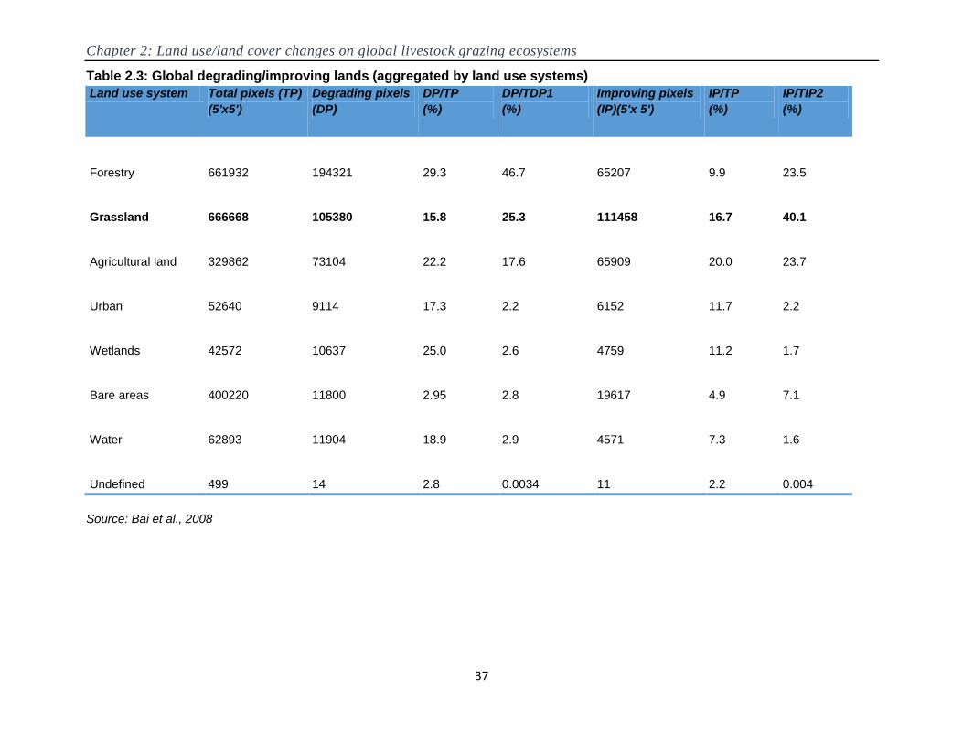
Chapter 2: Land use/land cover changes on global livestock grazing ecosystems
37
Table 2.3: Global degrading/improving lands (aggregated by land use systems)
Land use system Total pixels (TP)
(5'x5')
Degrading pixels
(DP)
DP/TP
(%)
DP/TDP1
(%)
Improving pixels
(IP)(5'x 5')
IP/TP
(%)
IP/TIP2
(%)
Forestry 661932 194321 29.3 46.7 65207 9.9 23.5
Grassland 666668 105380 15.8 25.3 111458 16.7 40.1
Agricultural land 329862 73104 22.2 17.6 65909 20.0 23.7
Urban 52640 9114 17.3 2.2 6152 11.7 2.2
Wetlands 42572 10637 25.0 2.6 4759 11.2 1.7
Bare areas 400220 11800 2.95 2.8 19617 4.9 7.1
Water 62893 11904 18.9 2.9 4571 7.3 1.6
Undefined 499 14 2.8 0.0034 11 2.2 0.004
Source: Bai et al., 2008

Chapter 2: Land use/land cover changes on global livestock grazing ecosystems
38
Bai et al. (2008), however, identify land improvement under various land use/land cover classes
(Tables 2.3and 2.4). Grasslands are demonstrated to account for the largest improved areas
globally; 40.1% of the improved areas were found in grasslands. The improvement represented
16.7% of the grassland areas. Contrary to degradation, grazed areas indicated much
improvement compared to the natural and protected grasslands and the indication that
anthropogenic factors do not always lead to degradation effects.
Table 2.4: Global degrading and improving areas by land use systems
Land use systems
Total
pixels(TP)
Degrading
pixels (DP) DP/TP(%)
Improving
pixels (IP)
IP/TP
(%)
Herbaceous - not managed/natural 212858 19012 8.9 17870 8.4
Herbaceous - protected areas 76707 10435 13.6 8560 11.2
Herbaceous with extensive pastoralism 154528 33253 21.5 31181 20.2
Herbaceous with moderate/intensive
pastoralism 129382 23199 17.9 33376 25.8
Herbaceous with intensive pastoralism 93193 19481 20.9 20471 22
Source: Bai et al., 2008.

Chapter 2: Land use/land cover changes on global livestock grazing ecosystems
39
Figure 2.2: The areas of NDVI improvement
Source: Le et al. (2014)

Chapter 2: Land use/land cover changes on global livestock grazing ecosystems
40
2.6 Are all grazing land losses productive losses?
The short answer is no. The analysis in the previous sections indicates that degradation is
mainly a management issue. Better management of grasslands is associated with less
degradation (Table 2.4). Degradation of grasslands is likely to occur where conversions of some
part of the ecosystems occur and no additional management action is taken on the remaining
grazing areas. This is illustrated in developing countries such as Africa under extensive grazing
systems. With increasing human and livestock populations, diminishing grazing resources play a
big role in determining the intensities at which grazing resources are exploited in the developing
world (Kiage, 2013). This is in support of Mannetje (2002), who indicates that among the key
causes of degradation in (semi-)arid rangelands in developing countries is the loss of the
ecosystems to other uses such as cultivation. With hardly any adoption of intensive production
systems, loss of grazing areas may present various problems: (1) less forage becomes available
with declining grazing areas; (2) the ecosystems are used more intensively creating room for
degradation with less vegetation cover and less palatable grasses; and (3) with less forage
available, conflicts are likely to arise between different groups, such as conflicts between
cultivators, pastoralists, and wildlife (Kiage, 2013; Eva et al., 2006; Tappan et al., 2004). Loss of
grazing land leads to a decline in forage availability and restricted mobility, and this results in the
overuse and degradation of the remaining grasslands (Eva et al., 2006; Mannetje, 2002;
Homewood et al., 2012; Flintan, 2011; Campbell et al., 2003; Campbell et al., 2005; Butt, 2010).
Loss of grasslands is also associated with degradation when losses occur to shrublands/steppes
and bare vegetation cover (Kitzberger and Veblen, 1999; Admasu, 2008; Tappan and Matthew
Cushing, 2013; Mlunga and Gschwender, 2015; Tappan et al., 2004). Invasive shrubland
vegetation are in most cases of lesser biological productivity and lead to a reduction of prime
grazing lands and thus are not considered as land improvement (Bai et al., 2008; Admasu,
2008; Mlunga and Gschwender, 2015). In addition, as observed in West Africa, harsh climatic
conditions in combination with other factors, such as overgrazing and topography, are observed
to lead to increased bare ground in pastoral areas (Tappan and Matthew Cushing, 2013;
Tappan et al., 2004).
However, not all conversions are associated with degradation. Conversion of native grasslands
to highly modified/improved grazing lands (pastures) as observed in Australia is not only
associated with increased productivity but may also lead to better management of the
ecosystems (Lesslie et al., 2011). In addition, as observed in Argentina and Uruguay, adoption
of better technologies may lead to conversion of native grasslands to pastures and croplands
with little adverse effects on the remaining native vegetation (Salazar et al., 2015; Baldi and
Paruelo, 2008). In fact, native grasslands in these two countries were observed to transit to
forests (afforestation), which are of high natural value. Even so, it should be noted that
conversion of native pastures to more intensive land uses such as modified/improved pastures
may be trading short-term increases in productivity for long-term losses in the capacity of the
resources to sustain productivity as well as other ecosystem services (Foley et al., 2005).
Intensive land uses such as farming on grasslands is associated with increased invasive species
at the expense of the number and abundance of native species, a decline in diversity and
abundance of biodiversity such as wildlife, and soil productivity losses, among others (Maitima et

Chapter 2: Land use/land cover changes on global livestock grazing ecosystems
41
al., 2009, Foley et al., 2005; Greiner et al., 2013). Many of the above are important for
agricultural production and thus imply that productivity is likely to be affected in the long term.
From the gains perspective, better management of land, as demonstrated in Europe and in
Montane Mainland Southeast Asia, may lead to increases in grasslands as well as other natural
vegetation at the expense of agricultural land (Fuchs et al., 2015a; Fox and Vogler, 2005). As
highlighted earlier, conversion of agricultural land to shrub and/or herbaceous vegetation and
other natural and/or semi natural land has occurred as a result of the countries‘ effort to fulfil
their biodiversity goals and preserve nature (Feranec et al., 2007; Fox and Vogler, 2005).
Contrariwise, increased grasslands are also not always associated with better management of
the ecosystems. This is well demonstrated in Central Asia, where increases in natural
vegetation, such as grassland and shrubland, resulted from abandoned farmland (Chen et al.,
2013). The abandoned lands in most instances are of poor quality and degraded from salt
accumulation among other factors and thus do not necessarily translate to better management
of land (Kitamura et al., 2006).
2.7 Conclusion
In spite of providing essential ecosystem goods and services, rangelands continue to be
degraded. Understanding rangeland dynamics and the paths of degradation is critical in the
design of sustainable rangeland use. The analysis on LULCC in global livestock grazing
systems indeed indicates that, despite native grazing lands being globally vast, the ecosystems
are on a decline. Globally, rangelands are undergoing various transformations which, in most
instances, involve losses to other land uses/covers. Expansions of agricultural land, invasive
vegetation, urban areas, and in some instances bare land cover are overriding these
ecosystems. Although some conversions are related biophysical factors such as climatic factors,
the key driving forces behind native grazing lands conversions are related to human activities.
This study presents a balanced picture by demonstrating that not all losses of native rangelands
are pessimistic and not all gains are associated with better managed systems. Despite some
transformations being linked to degradation of the ecosystems, such as invasive bush
vegetation, increased bare cover, and reduced productivity of the ecosystems, some
transformations involve productive gains.
Increasing population pressures coupled with improved technology, changing opportunities
brought about by markets, and changes in social organizations and attitudes have, in many
cases, resulted in the loss of grazing areas to cropping and pastures, with observable negative
effects on the remaining rangelands. While such conversions may involve increased productivity
of the introduced land use/land covers, caution should be taken to ensure sustainability of the
landscapes. The transformations should not sacrifice the long-term ecosystem services, the
resilience of the remaining grazing areas, or the modified landscapes. On a more positive note,
the study observed that, in some parts of the world, conservation efforts coupled with better
management of land have resulted in gains in grazing areas from other land covers other than
forests, which are of high natural value.
Effective and better management of native grazing lands would be beneficial not only from an
economic point of view but would also safeguard the capacity of the ecosystems to provide the
larger biosphere‘s goods and services such as protection of the soil and serving as carbon

Chapter 2: Land use/land cover changes on global livestock grazing ecosystems
42
sinks. As such, this paper supports the need of policy measures to ensure better management
of native grazing systems, including minimizing undesirable conversions. Where transformations
of the ecosystems are inevitable, the study supports the placement of strategic measures to
ensure sustainability of both the remaining native ecosystems and the modified landscapes. This
may include adoption of technologies such as conservation agriculture and production of good
quality forages adapted to grazing and drought stress.

43
Chapter Three
3 Determinants of Land Degradation and Improvement in
Kenyan Rangelands
3.1 Introduction
Kenyan rangelands are found in arid and semi-arid lands (ASALs) and comprise over 80% of the
country‘s total area (Harding and Devisscher, 2009; Kameri-Mbote, 2005; GOK, 2012a). The
ecosystems provide critical livelihood resources to over 20% of the total human population
residing in these areas (GOK, 2012a; Kameri-Mbote, 2005). Extensive pastoral systems of land
use prevail in the ASALs. Pastoralism not only feeds the millions in the system but also makes
significant contributions to the environment (Flintan, 2011).
Rangelands also play a key role in the economic development of the country. The ecosystems
support livestock and wildlife predominantly through their role as a natural resource
management system (GoK 2012a; Harding and Devisscher, 2009). Over 90% of the wild game
that supports wildlife tourism is found in rangelands (GoK, 2012a). In addition, in total,
approximately 70% of the national livestock are found in ASALs, with more than 80% of the
locally produced beef coming from the pastoral communities (Behnke and Muthami, 2011; GoK
2012a; Kameri-Mbote, 2005; Mwagore, 2003). Recent research estimates indicate that the
contribution of livestock to agricultural GDP was about Kshs. 320 billion (4.54 billion US dollars)
in the year 2009 (Behnke and Muthami, 2011). The amount was slightly less than that from
crops and horticulture with a contribution of $5.25 billion US dollars (Behnke and Muthami,
2011). This underscores the importance of maintaining the productivity of the resource base for
purposes of national development. Rangelands also serve as an important biodiversity
conservation area crucial for tourism, research, and national heritage (Maitima et al., 2009;
Mireri et al., 2008; Flintan, 2011; Harding and Devisscher, 2009).
The majority of the people living in ASALs are poor, the contributing factors being vulnerability to
drought, marginalization, poor infrastructure, and long distances to markets (GOK, 2012a;
Campbell et al. 2003). In addition, various processes over the years have impaired the dryland
ecosystems, through degradation, setting the rangeland communities further into poverty and
destitution. Estimates from research indicate that over the period 1982–2006, 18% of grasslands
and 42% shrub-lands in the country have experienced persistent decline in biomass productivity
(Le et al., 2014). This has been at the expense of livestock production, livelihood strategies, and
biodiversity (Maitima et al., 2009; Campbell et al., 2003).

Chapter 3: Determinants of Land Degradation and Improvement in Kenyan Rangelands
44
Figures 3.1 and 3.2 present the areas experiencing significant biomass productivity changes
across rangelands in the country between the period 1982 and 2006.
Figure 3.1: Distribution of degraded grassland and bushland pixels in rangelands
Data Source: (Le et al., 2014)1.
Figure 3.1 shows the rangeland areas experiencing persistent significant biomass productivity
declines across grazing vegetation: grassland and shrubland land cover/use types. The areas
with significant NDVI declines range from 0% to 12.82% of the administrative area (sub-
location). Figure 3.2 presents the areas showing significant positive biomass productivity
changes within the study areas.
1Rangelands defined as per FEWS livelihoods zones data for Kenya and are available at: http://www.fews.net/east-
africa/kenya/livelihood-zone-map/march-2011. See appendix A for the livelihoods zones map
Wajir
Marsabit
Turkana
Garissa
Isiolo
Tana River
Mandera
Narok
Kajiado
Samburu
Laikipia
Baringo
West Pokot
40°0'0"E
40°0'0"E
35°0'0"E
35°0'0"E
5°0'0"N 5°0'0"N
4°0'0"N 4°0'0"N
3°0'0"N 3°0'0"N
2°0'0"N 2°0'0"N
1°0'0"N 1°0'0"N
0°0'0" 0°0'0"
1°0'0"S 1°0'0"S
2°0'0"S 2°0'0"S
3°0'0"S 3°0'0"S
NDVI Decline
Degraded shrub land
Degraded grassland

Chapter 3: Determinants of Land Degradation and Improvement in Kenyan Rangelands
45
Figure 3.2: Distribution of areas with significant positive biomass productivity changes
Data Source: (Le et al., 2014).
Unlike the degraded areas, the data on areas with improved biomass productivity is not
classified under various land use/land cover types. This presents a challenge in identifying
whether the areas present grazing vegetation covers. In addition, invasive species such as P.
juliflora are indicated to have colonized large parts of the ASALS areas where improved
productivity is shown (Fig 3.2; Sirmah et al. 2008). With no grounding-truthing exercises of the
dataset to verify the vegetation cover, the above challenges complicate possible analyses on
improved vegetation cover.
Adequate policy action is needed to mitigate the adverse effects of rangeland degradation on
the capacity of the ecosystems to provide essential ecosystem goods and services. Effective
policy can be enhanced through an understanding of the factors driving land degradation as well
as those enhancing sustainable rangeland management (SLM) (Campbell et al., 2003; Liniger et
al., 2011; Akhtar‐Schuster et al., 2011; Nkonya et al. 2013). This information is crucial for the
planning, management, and conservation of the rangeland natural resources. Although general
drivers of land degradation and SLM practices have been identified (Lambin et al., 2003; Vlek et
al., 2008; Nkonya et al. 2011; Liniger et al., 2011; Akhtar‐Schuster et al., 2011; von Braun et al.,
2013; Nkonya et al. 2013), comprehensive analyses of the factors and their causality in different
Wajir
Marsabit
Turkana
Garissa
Isiolo
Tana River
Mandera
Narok
Kajiado
Samburu
Laikipia
Baringo
West Pokot
40°0'0"E
40°0'0"E
35°0'0"E
35°0'0"E6°0'0"N 6°0'0"N
5°0'0"N 5°0'0"N
4°0'0"N 4°0'0"N
3°0'0"N 3°0'0"N
2°0'0"N 2°0'0"N
1°0'0"N 1°0'0"N
0°0'0" 0°0'0"
1°0'0"S 1°0'0"S
2°0'0"S 2°0'0"S
3°0'0"S 3°0'0"S
Legend
Others
Improved Areas
Chapter 3: Determinants of Land Degradation and Improvement in Kenyan Rangelands
46
contexts is hardly sufficient to provide credible and policy-relevant scientific information (von
Braun et al., 2013; Nkonya et al., 2013).
At the global and regional levels, the identified causes of land degradation are mainly based on
expert opinions with less empirical analyses assessing the relationship between land
degradation and the selected variables (Oldeman et al., 1990; Barbier, 1997; Bregas, 1998;
Lambin et al., 2001; Lambin et al., 2003; Ravi et al., 2010; von Braun et al., 2013; Vlek et al.,
2008). Similar observations are made with regard to factors enabling SLM practices in which
analyses are mainly qualitative (Akhtar‐Schuster et al., 2011; Liniger et al., 2011; Reed et al.,
2011; Nkonya et al., 2013). Among the identified factors likely to promote SLM practices in
rangelands and vice versa are the need to integrate pastoralists and other relevant stakeholders
in efforts towards effective management of rangelands (Reed et al., 2007; Poulton and Lyne,
2009; Homewood et al., 2012; Hobbs et al., 2008; Upton, 2010; Liniger et al., 2011); recognition
of traditional institutions in the management of rangeland resources (Reed et al., 2007; Nkonya
et al., 2011; Westoby et al., 1989; Solomon et al., 2007; Angassa and Oba, 2008); knowledge
constraints (Liniger et al., 2011; Akhtar‐Schuster et al., 2011; Reed et al., 2011; von Braun et al.,
2013); the need for policy to move away from protection/conservation to sustainable use of the
natural resources with direct benefits to households (Shaoliang and Muhammad, 2011; Mekuria
and Yami, 2013; Dorj et al., 2013); inadequate and poor-quality services ranging from lack of
extension support to all weather roads (Neely et al., 2009; Liniger et al., 2011) ; market failures
(Markelova et al., 2009; Ahuya et al., 2005; Aklilu, 2002; Hurrissa and Eshetu, 2002;
Duraiappah, 1998; Hatfield and Davies, 2006; von Braun et al., 2013); institutional failures and
institutional capacity constraints (Liniger et al., 2011; Akhtar‐Schuster et al., 2011; Reed et al.,
2011; Kirsten et al., 2009a; Meinzen-Dick and Mwangi, 2009; Kerven et al., 2012; Chavunduka
and Bromley, 2011; Bruce et al., 1994; Amman and Duraiappah, 2004; von Braun et al., 2013);
conflicts (Bromwich, 1980; Osman-Elasha and El Sanjak, 1980); poverty and financial
constraints (Nkonya, 2008; Barbier, 1997; Duraiappah, 1998; Liniger et al., 2011; Akhtar‐
Schuster et al., 2011; Reed et al., 2011; Kerven et al., 2012; von Braun et al., 2013); the need to
diversify the means of sustaining livelihoods to lessen pressure on rangelands (Coppock et al.,
2011; Jian, 2011); power, wealth, and greed (Duraiappah, 1998; Nunow, 2011); and low
economic benefits associated with traditional pastoralism (Kamara et.al, 2004; Alston et al.,
1995; Campbell et al., 2005; Behnke, 1985; Hatfield and Davies, 2006). Where empirical
analyses on drivers of land degradation have been made, only correlation relationships between
land degradation proxies and selected biophysical and socioeconomic variables have been
analyzed, with no strong causal relationships identified (Nkonya et al 2011).
Similar observations are made in the majority of the local case studies in which analyses are
mainly qualitative (Turner, 1999; Ayoub, 1998; Douglas, 2006). In Kenya, there is ample
qualitative research on land degradation in drylands (Flintan, 2011; Pickmeier, 2011; Temper,
2012; Homewood 2012; Hobbs et al., 2008; Meinzen-Dick and Mwangi, 2009; Mwangi, 2009;
Mireri et al., 2008; Harding and Devisscher, 2009). Only a few empirical studies on drivers of
rangeland degradation have been performed, with hardly any on the determinants of SLM
practices (Kiage et al., 2007; Serneels and Lambin et al., 2001; Maitima et al., 2009; Greiner et
al., 2013). In addition, the main focus of these studies is on land cover/use change, with no
causal association to land degradation or SLM practices. Thus, there is a need for analyses on

Chapter 3: Determinants of Land Degradation and Improvement in Kenyan Rangelands
47
the determinants of land degradation and SLM practices to move from simplistic explanations
and single-cause relationships to quantitative analyses that integrate multiple causes while
identifying the causal relationship (Lambin et al., 2003; Nkonya et al 2011). In addition, the
causal relationships should be carried out within social–ecological strata, such as land use
zones (in this case rangelands), for more insightful analyses (Vlek et al., 2008; Sommer et al.,
2011; Vu et al., 2014). Based on the above and data availability issues, this paper aims at
identifying the causal relationship of the biophysical and socio-economic factors affecting SLM
practices in rangelands at the national level in Kenya.
To lay ground for the analysis, the study first presents a brief review of key rangeland
degradation components, the main drivers and the corresponding consequences of rangeland
degradation in Kenya in Section 3.2. Thereafter, the study presents the conceptual and empirical
frameworks in Section 3.3. Section 3.4 outlines the study area, data, and analysis methods.
Presentation of the analyses results follows in Section 3.5, followed by a discussion of the
results in Section 3.6. Finally, the conclusion and policy implications are presented in Section
3.7 of the study.
3.2 Key Rangeland Degradation Components, Drivers, and Corresponding
Consequences in Kenya
3.2.1 Rangeland degradation components
As highlighted earlier, rangeland environments in Kenya are mainly found in ASALs and
represent over 80% of the country‘s total area (Harding and Devisscher, 2009; Kameri-Mbote,
2005; GOK, 2012a). ASALs on average have rainfall ranging from 300-800 mm annually and are
found in agro climatic zones IV, V, and VI (Orodho, 2006; Sombroek et al., 1982). The dominant
soils in ASALs of Kenya include Yermosols, Xerosols, Lithosols, Regosols, Solonetz,
Solonchaks, Luvisols, Lixisols, Acrisols, Alisols, Ferralsols, Planosols, Vertisols, and Fluvisols
(Biamah, 2005). These soils are characterized by structural instability, high levels of salinity and
sodicity, poor drainage, soil crusting and compaction, very low inherent fertility, and complete
lack of moisture and vegetation all year round (Biamah, 2005). The range areas are further
characterized by high temperatures and frequent wind storms, making the soils very vulnerable
to degradation (Orodho, 2006). Degradation of the national range areas manifests itself mainly
in the form of soil erosion, vegetation cover conversions, soil salinity, and physical degradation
by trampling, especially around watering points (Odhengo et al., 2012; Gomes, 2006;
Duraiappah et al., 2000; Mwagore, 2003; Mugai, 2004; Maitima et al., 2009; Greiner et al.,
2013).
Poor protective cover of the soils brought about by vegetation clearing, overgrazing, and
trampling along livestock tracks increases the vulnerability of the soils to soil erosion. These
processes leave the land bare and soil exposed during periods of heavy wind or rain, thus
encouraging runoff (Mwagore, 2003). With reduced cover, bare soils erode easily, leading to
losses of fertile top soils (Maitima et al., 2009). Soil erosion may appear either in the form of
splash erosion, sheet erosion, rill erosion, gully erosion, or wind erosion (Mwagore, 2003). In
addition to soils eroding easily, removal of plant cover leads to low replenishment of soil
nitrogen, phosphorous, potassium, soil organic matter, and high evaporation water losses
(Maitima et al., 2009; Biamah, 2005).

Chapter 3: Determinants of Land Degradation and Improvement in Kenyan Rangelands
48
Other than soil erosion, vegetation degradation is a key problem facing rangelands in the
country. Over the years, succulent bushes and thorny shrubs have been on the increase in
range areas at the expense of palatable grasses. Palatable perennial grass species such as T.
triandra are on the decrease with the replacement of bare ground cover and unpalatable grass
species such as H. schimperi, A. adoensis and, Microchloa kunthii (Orodho, 2006; Olang, 1988).
Vegetation cover is also changing from grassland to bush with the encroachment of woody
plants such as Dodonaea angustifolia var. viscosa, Tarchonanthus camphoratus, Prosopis
juliflora, and Acacia drepolobium (Olang, 1988; Flintan, 2011; Greiner et al., 2013). Removal of
natural woody savannah grassland vegetation is associated with invasive shrub vegetation
(Greiner et al., 2013).
Salinity is another problem facing ASALs, and it occurs due to either natural or anthropogenic
causes (Mugai, 2004; Maitima et al., 2009). Natural processes forming saline salts are
accelerated by the removal of natural vegetation (Mugai, 2004). Clearance of deep-rooted native
vegetation with the replacement of shallow-rooted vegetation causes a rise in the water table of
the soils, thus mobilizing salts in the soil (Mugai, 2004). Accumulation of salts at the surface
affects the productivity of the land, killing the protective plant cover. This leaves the land bare
and vulnerable to soil erosion.
Physical degradation of rangelands by trampling, especially around watering points, is also
common in the country‘s rangelands (de Leeuw et al., 2001). Attraction to scarce and declining
rangeland water resources contracts rangeland activities into isolated pockets, especially during
prolonged drought periods, resulting in trampling. The influx of pastoralists along watering points
increases pressure on river banks, leading to degradation by trampling and overuse of pasture
resources (Pickmeier, 2011; Gomes, 2006).
3.2.2 Drivers of Rangeland Degradation
Globally, there is high variability in biophysical factors and human-related activities associated
with land degradation (Lambin et al., 2003). Efforts geared towards mitigating or halting land
degradation therefore require an understanding of the various causes in specific contexts.
Human-related factors, also known as anthropogenic factors, affect the biophysical state
attributes, such as soils, biomass, and vegetation community structure through land use, defined
as the manner in which the biophysical attributes of land are manipulated and the intent of that
manipulation (Lambin et al., 2003; Lambin et al., 2006). Insights into the anthropogenic drivers
of rangeland degradation are hence crucial in counteracting rangeland degradation.
Understanding the biophysical drivers of rangeland degradation is also essential as they define
the natural capacity for land use changes (Lambin et al., 2003). Based on a review of the
literature of the various determinants of land degradation in range areas in Kenya, we categorize
the key drivers into three main groups: institutional, socio-economic, environmental, and physical
variables.
3.2.2.1 Institutional Variables
The pressure points which have had the greatest impact on pastoral land management have
been the land reforms codifying individual rights to resources that were formerly used collectively
under common property arrangements (Mwangi, 2009; Meinzen-Dick and Mwangi, 2009;
Duraiappah et al., 2000; Campbell et al., 2003; Kameri-Mbote, 2005; Mwagore, 2003).

Chapter 3: Determinants of Land Degradation and Improvement in Kenyan Rangelands
49
Recognition of economic opportunities with altered land holding systems coupled with the belief
that mobile pastoralism was irrational and environmentally destructive has contributed to the
motivation for subdivision of rangelands into individual holdings (Campbell et al., 2003; GOK,
2012a).
The transformations in land tenure have resulted in fragmented rangelands, a key cause of
rangeland degradation (Flintan, 2011; Rutten 1992; Galaty and Ole Munei, 1999; Amman and
Duraiappah, 2004). Fragmented rangelands result in the loss of flexibility, thus disrupting
seasonal movements of livestock (Flintan, 2011). Restricted mobility leads to loss of the
opportunistic spread of grazing pressure, leading to overuse of resources in the confined areas
(Boone and Hobbs, 2004; Hobbs et al., 2008; Meinzen-Dick and Mwangi, 2009). This
undermines the capacity of pastoral communities to sustainably use the ecosystems as well as
deal with risks such as droughts. On the contrary, Lesorogol (2005) found that individual rights
to pastoral resources have resulted in gains for pastoral communities. The benefits emanate
from the role privatization plays in diversifying means of livelihoods in which crop farming is a
supplement to livestock production.
Land alienations for private interests is another factor affecting the resource base of livestock
with negative consequences on the land within confined areas. With land ownership in most
rangelands falling either as trust or government land, elite segments of the Kenyan society and
private developers have been allocated large tracts of land illegally near bodies of water as it is
with the Tana Delta (Pickmeier, 2011). In other areas, pastoralists have been limited in the drier
parts of range areas, with the remaining areas restricted for use by private undertakings. For
instance, in Laikipia County, most pastoralists are limited in the drier northern parts covering
7.45% of the county, with 48 individuals privately controlling 40.3% of the rest of the land as
commercial ranches or conservancies and 23 large-scale farms covering 1.48%. The individual
properties are fenced off and rarely provide migration routes for pastoralists, thus limiting their
mobility (Flintan, 2011). Development projects such as dam constructions and large-scale
irrigation schemes have also alienated large tracts of land from common ownership, thus limiting
grazing areas (Pickmeier, 2011; Nunow, 2011; Temper, 2012).
Inappropriate development policies such as those encouraging increased permanent watering
points in pastoral drylands have been observed to result in degradation (Gomes, 2006). For
instance, increased borehole development in ASALs attracts permanent settlement of
pastoralists. Sedentarization of pastoral communities negatively affects vegetation productivity in
range areas reducing ground cover and thus increases the vulnerability of the soils to soil
erosion (Butt, 2010). In addition, conservation protectionism policies in some cases have been
observed to lead to marginalization of pastoralists despite their ability to live successfully with
wildlife. For instance, some policies such as those invariably encouraging wildlife activities to
replace pastoralism instead of the two co-existing may emerge as a threat competing for
pastoral land, restricting livestock mobility and access to pastoral resources which are necessary
for sustainable rangeland use (Homewood, 2012; Flintan, 2011; Campbell et al., 2003; Campbell
et al., 2005).
Chapter 3: Determinants of Land Degradation and Improvement in Kenyan Rangelands
50
3.2.2.2 Socio-Economic Variables
Important changes in ASALs have been observed with the expansion of crop farming, especially
in wetter rangeland areas (Pickmeier, 2011; Temper, 2012). In addition to changes in land
tenure, the expansion of agriculture has been supported by the expansion of market
opportunities for crop production, both for local consumption and for export (Campbell et al.,
2005; Duraiappah et al., 2000). With the encroachment of crop farming, four forces cause
degradation in these resource bases. The first is the inevitable overgrazing by pastoralists driven
into small, drier grazing areas, but still maintaining large herds of livestock (Duraiappah et al.,
2000; Kameri-Mbote, 2005). Better-watered locations provide important ecological functions
during dry seasons. These dry-season grazing areas form part of the sustainable grazing cycle,
as they relieve grazing pressures on the wet season grazing areas (Temper, 2012; Mireri et al.,
2008). Loss of the well-watered areas to crop farming means lack of relief of the wet season
grazing areas in dry seasons, subjecting the areas to serious environmental degradation through
depletion of biomass, loss of biodiversity, and soil erosion (Mireri et al., 2008; Mwagore, 2003).
Second, commercial farmers leasing land in rangelands have little incentive to make
conservational investment measures on leased parcels. Once the leased parcel becomes
unproductive, the commercial farmers shift and lease other parcels, creating ‗dustbowl‘
conditions (Duraiappah et al., 2000). In addition, continued cultivation of rangelands results in
much drier soils subject to soil erosion (Gachimbi, 2002). Third is the degradation by salinization
caused by the irrigation of unsuitable soils and the replacement of deep-rooted natural
vegetation by shallow crops (Gachimbi, 2002; Mugai, 2004). The fourth factor is nutrient mining
caused by continued cultivation of the ecologically unsuitable land (Mwagore, 2003; Gachimbi,
2002).
Poverty is also observed to be a likely force driving rangeland degradation. Rangelands have
the lowest development indicators and the high levels of poverty in the country (GOK, 2012a).
The high incidence of poverty limits the pastoral communities‘ capability of mitigating their
vulnerability to drought. To reduce livestock mortality during critical periods, pastoralists are
observed to keep large numbers of livestock. Their goal is to maintain sufficient livestock in the
face of an unpredictable physical environment. This is, however, a self-defeating mechanism, as
the large number of livestock increases grazing pressure on marginal lands exacerbating
livestock mortality. This sets the pastoral communities in a downward spiral of poverty
(Duraiappah et al., 2000; Campbell et al., 2005). Poverty is also associated with the continued
dependence on the natural resources with little adoption of appropriate technologies to increase
productivity of the ecosystems in a sustainable way.
The increasing number of people searching for economic security with the growing population in
the country is among the factors causing intense pressure on the pastoral natural resources
(Mwagore, 2003). With the increasing population growth, rangelands serve as sinks for migrating
farmers from the high-potential areas, leading to increased competition for pastoral resources
(Kameri-Mbote, 2005; Campbell et al., 2005; Mwagore, 2003). On the other hand, Tiffen and
Mortimore (1994) showed that population increase may compel the society to adapt
mechanisms in response to challenges presented by increased pressure on land. Increased
population may stimulate investments in intensification technologies to restore and improve the
land resource base with the increasing population (Tiffen and Mortimore, 1994).

Chapter 3: Determinants of Land Degradation and Improvement in Kenyan Rangelands
51
Increasing livestock densities is also an important factor driving rangeland degradation in the
country. The population of livestock has also been on the increase with the increasing pastoralist
population. An additional contributing factor to increased livestock densities are sales/leases of
pastoral land in the exchange of livestock at a time when access to pastoral resources is on the
decline (Duraiappah et al., 2000; Rutten, 1992). The adverse effect of increasing livestock
densities accompanied by the loss of rangelands is further exacerbated by inadequate
participation in markets by pastoralists (Rutto, 2014). As competing land use increases, the
ability of livestock keepers to respond to potential increases in demand for livestock in livestock
markets would relieve pressure on rangeland resources.
Disregard for indigenous knowledge and rangeland management strategies of pastoralists is
also another factor leading to the degradation of rangelands. De-emphasizing the links and
relationships between people, their culture, and resources has contributed to unsustainable
practices in the management of environmental and natural resources (Mwagore, 2003). For
instance, traditionally pastoralists developed an efficient system for managing resources to deal
with the erratic rainfall characterizing the drylands. Herds were moved between dryland wet-
season pastures, making use of the scattered rangeland resources on a large scale (Duraiappah
et al., 2000; Campbell et al., 2005; Meinzen-Dick and Mwangi, 2009). As previously mentioned,
restricted herd mobility has negative effects on the ecological sustainability of the pastoral
resources. These observations are supported by empirical studies showing a pronounced
positive relationship between cattle mobility and resource availability during dry periods,
indicating the importance of mobility to resource access (Butt, 2010). In addition, the study
revealed that livestock used different parts of the ecosystem at different times.
3.2.2.3 Environmental and Physical Variables
Climate is an important factor affecting productivity of rangelands in ASALs. Drought is a
recurrent phenomenon that affects large areas and numbers of people living in ASALs in the
country (Harding and Devisscher, 2009). During drought years, the natural production capacity
of the range areas reduces, leading to pastoral communities exploiting vulnerable environmental
resources, such as along water points, in order to meet livelihood needs. The intensive influx of
livestock and wildlife concentrated around a few water points leads to severe vegetation and soil
degradation processes (Mwagore, 2003; Pickmeier, 2011).
Additional biophysical factors affecting rangelands are land characteristics such as soil
characteristics and terrain. The high temperatures and frequent wind storms in these areas
further exacerbates the vulnerability of the ecosystem to degradation (Orodho, 2006). These
factors combined make the areas inherently susceptible to degradation compared to other
geographical areas in the country.
Drawing from the above discussions, the drivers of rangeland degradation emerge to be highly
interrelated with externalities running from one factor to another. The study therefore recognizes
the challenge of generalizing drivers into simple categories: under the simple generalizations,
interactions of factors do come to play.

Chapter 3: Determinants of Land Degradation and Improvement in Kenyan Rangelands
52
3.2.3 Consequences of Rangeland Degradation
There are various consequences of rangeland degradation in relation to humans, animals,
water, soils, and the national development of the country.
Loss of ecological functions of degraded range areas has resulted in catastrophic social and
economic losses in the past (Kay, 2012). With degradation of rangelands, the pastoral resources
become less and less productive, resulting in the loss of livestock to hunger or quality decline,
especially during drought seasons (Duraiappah et al., 2000; Mireri et al., 2008; Maitima et al.,
2009). Cattle mortality is estimated to rise as high as 3 million cattle countrywide, leading to
losses of about $1 billion (Western, 2009; Flintan, 2011) during a drought year. The losses
incurred could be significantly higher as the estimates exclude mortality of other livestock such
as sheep and goats. Loss of livestock coupled with a drop in value of degraded land results in
the decrease of the income levels of pastoralists, pushing the communities further into poverty
(Duraiappah et al., 2000). In addition, declining productivity of rangelands increases the
vulnerability of the rural households to shocks from variable climates (Galaty and Ole Munei,
1999; Amman and Duraiappah, 2004; Mwagore, 2003). Loss of coping mechanisms during
droughts also results in high loss of human life and huge expenditures of humanitarian relief,
reaching heights of over of $4.0 million (Kay, 2012; Flintan, 2011).
Competition over limited and declining rangeland resources has compounded conflicts among
cultivators, pastoralists, and wildlife in the range areas of the country (Kay, 2012; Orindi et al.,
2007; Mogaka, 2006; Pickmeier, 2011; Maitima et al., 2009). Due to insecurity, pastoralists
concentrate in some areas thought to be secure, leaving other pastures unused. The limited
mobility further exacerbates the unsustainable use of the range areas, with livestock becoming
more subject to diseases (Orindi et al., 2007; Notenbaert, 2007; Gomes, 2006). Prolonged and
regular conflicts result in loss of wildlife, livestock, and human life. Incomes are also lost with
closure of markets and with grazing areas becoming no-go zones (Flintan, 2011).
Rangeland degradation also has negative effects on biodiversity. Trends in economically useful
plants over time have been on the decline with intensification of land use and the subsequent
negative consequences on the ecological function of rangelands (Maitima et al., 2009). In
addition, empirical studies show a strong negative correlation between soil erosion severity and
plant species numbers (Maitima et al., 2009). Additionally, wildlife in some ASALs in the country
is on a strong decline, with losses in some regions reaching as high as over 50 percent between
the years 1970 and 1990 (Maitima et al., 2009). Among the key causes of wildlife decline is
pasture scarcity, emanating from a loss of habitat through land fragmentation and conversion to
cultivation and the resulting ecological instability of rangelands (Maitima et al., 2009; Harding
and Devisscher, 2009; Homewood, 2012). In addition, loss of wildlife is observed as a
consequence of human wildlife conflict, exacerbated by movement of wildlife into people‘s
settlements as they look for water and pasture.
The off-site effects of rangeland degradation include effects on the tourism sectors,
sedimentation of water systems, and expenditure on meat imports. Loss of wildlife emanating
from degraded rangeland ecosystems has a negative impact on wildlife tourism, which is a major

Chapter 3: Determinants of Land Degradation and Improvement in Kenyan Rangelands
53
national development sector in the country. The tourism sector is the country‘s highest foreign
exchange earner, and it contributes about 12% to Kenya‘s GDP (GOK, 2012a). In addition, the
tourism sector contributes over half of the earnings from the restaurant and hotels sectors of the
country, and thus the decline of wildlife would have greater implication to the country as a whole
(Mogaka, 2006). With loss of flood plains and river banks to crop farmers, influx of pastoralists
on limited watering points causes sedimentation of water. Other than affecting negatively
aesthetic activities and exclusive settlements around water bodies, sedimentation reduces the
capacity and lifespans of water bodies and leads to ecosystem damage such as risk to marine
life (Mwagore, 2003).
Low productivity of rangelands is a contributory factor to Kenya‘s state of being a meat-deficit
country. The country imports about 25-30% of its beef through illegal movement of livestock from
neighboring countries (Muthee, 2006). Research suggests that if 50% of the domestic deficit
meat were to be met by increased livestock production from an ASAL region, for instance, the
North Eastern province alone, more than 400,000 jobs would be created, thus reducing
unemployment in the region by about 2.4% each year, and producers‘ incomes would increase
by more than Kshs 2 billion each year (Rakotoarisoa et al., 2008).
Livestock production plays a significant role in the economic development of the country
(Behnke and Muthami, 2011; GOK, 2012a). As highlighted earlier, value added by livestock to
agricultural GDP is significant and only slightly less than that of arable agriculture (Behnke and
Muthami, 2011). Degraded rangelands are therefore likely to have a negative impact not only on
livelihoods but also on the economy of the country. The total cost of milk and meat losses
associated with land degradation in the country were estimated to be about 2007 US$ 49.5
million and 2007 US$ 8.7 million, respectively, for the year 2007, with the highest costs occurring
in rangelands (ASALs) (Mulinge et al., 2016). When the costs associated with the weight loss of
animals not slaughtered or sold is included, the estimated costs related to land degradation were
estimated to be about 2007 US$ 77.9 million (Mulinge et al., 2016).
The above discussion underscores the urgent need to adopt SLM management practices in
rangelands.
3.3 Conceptual and Empirical Frameworks
3.3.1 Conceptual Framework
The conceptual framework for this study is based on the ELD conceptual framework (Nkonya et
al., 2011; von Braun et al., 2013; Nkonya et al., 2013; Figure 3.3). Drivers of land degradation
are classified into two groups: proximate and underlying drivers. Proximate drivers of land
degradation are those that directly affect land and involve physical action on land (Nkonya et al.,
2011; Lambin et al., 2003). Proximate drivers as shown in Figure 3.3 are further divided into
biophysical drivers and unsustainable land management practices. The underlying drivers of
land degradation refer to the indirect causes of land degradation. They are also known as root
causes, as they influence land use/cover through the proximate causes of degradation (Nkonya
et al., 2011; von Braun et al., 2013; Lambin et al., 2003). The drivers of land degradation
determine its level, which ultimately determines its outcomes/effects. Action can be taken,

Chapter 3: Determinants of Land Degradation and Improvement in Kenyan Rangelands
54
Levels of rangeland
degradation
Outcomes:
-Ecological effects
-Socio-cultural effects
-Production effects
-Economic effects
Underlying Drivers
E.g. institutional and
policy factors,
socioeconomic factors,
household characteristics
and preferences
Proximate Factors -Biophysical factors E.g. land characteristics, agro-ecological zones -Unsustainable land management practices E.g. unsustainable farm systems
Processes
Action against land
degradation
-SLM strategies
-Institutional and
policy settings
however, to halt or mitigate rangeland degradation (Figure 3.3). The action taken can be to
control either the causes of land degradation, the levels of degradation, or its effects (Nkonya et
al., 2011).
Source: Adapted from Nkonya et al. (2011) with modifications by the author
There exists ample empirical evidence that the factors driving land degradation are similar to
those inhibiting the adoption of SLM practices (Nkonya et al., 2016a; Shiferaw et al., 2009;
Prokopy et al., 2008). For instance, empirical studies show that decisions on the adoption of
SLM practices depend on biophysical environments such as the slope of land and agro
ecological zones (Pagiola, 1996; Pender et al., 2006; Gillespie et al., 2007; Kim et al., 2004).
Additional factors influencing adoption of best practices on natural resource management
include incentives such as input and output prices (Shiferaw and Holden, 1999; Shiferaw and
Holden, 2000; Pagiola, 1996); access to markets, production diversification and off-farm income
opportunities (Tiffen et al., 1994; Pender et al., 2006; Pender and Kerr, 1998; Gillespie et al.,
2007; Kim et al., 2004; Shiferaw and Holden, 1998); poverty, capital constraints, farm resource
assets, income, and wealth (Grepperud, 1997; Shiferaw and Holden 1999; Prokopy et al., 2008;
Kim et al., 2004; Gillespie, et al., 2007; Pender et al., 2006); human capital resource and other
household characteristics (Shiferaw and Holden, 1998; Pender and Kerr, 1998; Park and Lohr,
2005; Gillespie et al., 2007; Kim et al., 2004; Prokopy et al., 2008); land tenure (Shiferaw and
Figure 3.3: Conceptual Framework: Determinants of land degradation and SLM adoption

Chapter 3: Determinants of Land Degradation and Improvement in Kenyan Rangelands
55
Holden 1999; Ahuja, 1998); access to extension services, information asymmetry, and farmer
participation (Park and Lohr, 2005; Pender et al., 2006; Tiffen et al., 1994a; Gillespie et al.,
2007; Prokopy et al., 2008); and technology characteristics such as labor demand (Shiferaw and
Holden, 1998; Shiferaw et al., 2009).
Based on the synthesis of the SLM adoption literature and data availability issues, adoption of
SLM practices on Kenyan rangelands is conditioned on the identified factors.
3.3.2 Empirical Framework
To assess the determinants of SLM adoption on Kenyan rangelands, a binary probit model was
chosen due to the nature of the dependent variable which is measured on a binary scale:
if a household adopted SLM practices in rangeland management, and otherwise .
The observed decision ( ) is however assumed to represent a latent variable which
represents households' utility acquired from adopting SLM practices. is observed if the
underlying latent variable exceeds a certain threshold following the decision rule:
(3.1)
Adoption of SLM practices is specified as follows:
(3.2)
where
is adoption of SLM technologies
is a vector of biophysical factors (e.g. soil type, slope, agro-ecological zones)
is a vector of household characteristics (e.g. age, gender, education, household size)
is a vector of socio-economic factors and asset endowment (e.g. cultivable land,
livestock wealth, poverty, off-farm income)
is a vector of institutional and policy factors (e.g. extension services, credit facilities, land
tenure, market opportunities)
is a vector of vector district-fixed effects and
captures stochastic disturbances, assumed to be normally distributed.
Other than relying on the literature to correctly specify the model, the study carries out robust
checks to check for model misspecifications (Dimara and Skuras, 2003). The study also employs
instrumental variable (IV) estimation to address possible endogeneity issues likely to arise. The
1iY
0iY
iY *
iY
iY
*
iY
0
1iY
if
if
0
0*
*
i
i
Y
Y
ii uzxxxxY 5443322110 ),0(~; 2NIDui
Y
1x
2x
3x
4x
iz
iu
Chapter 3: Determinants of Land Degradation and Improvement in Kenyan Rangelands
56
robustness of the regression results is made by comparing the results of the probit model and
the instrumental variable (IV) estimations.
3.4 Study area, data, and analysis methods
3.4.1 Description of the Study Area
The study is conducted in thirteen counties in Kenya located in the dry lands (arid and semi-arid
lands [ASALs]) of the country. The counties include Turkana, Marsabit, Mandera, West Pokot,
Samburu, Isiolo, Wajir, Garissa, Baringo, Laikipia, Narok, Kajiado, and Tana River. The
production system in these counties is either largely pastoralism or agro-pastoralism (Fig. 1.7).
These counties are endowed with a variable climate and have the highest incidence of poverty
in the country (GOK, 2012a; Campbell et al., 2003; Orodho, 2006; Sombroek et al., 1982).
Livestock production remains the key component of agricultural production in these areas, with
pastures forming the main feed for livestock.
3.4.2 Data
The data set used in the analysis comes from the Kenya Integrated Household Budget Survey
(KIHBS) 2005/06, a national survey conducted in 2005/06 over a period of 12 months (KNBS,
2005/06a; KNBS, 2005/06b). The last national survey of this nature was conducted in the early
1980s (KNBS, 2005/06a). No current national surveys exist. The extensive dataset covers all
possible seasons and was drawn from each of the country‘s districts, including all ASALs
(KNBS, 2005/06a; KNBS, 2005/06b). A multistage sampling procedure was followed in the data
collection process. In the first stage, urban and rural clusters were drawn from each of Kenya's
70 districts. In total, the survey covered a total of 1,343 clusters (KNBS, 2005/06a; KNBS,
2005/06b). In the second stage, 10 households were selected, with equal probability from each
of the clusters, giving a total sample of 13,430 households. Of the total 13,430 households
sampled, 2190 households are within the focus area of the study. The geographical location of
all the households surveyed was captured using the Geographical Positioning System (GPS)
enabling their precise location. The KIHBS dataset provides detailed data on agriculture
holdings, agriculture input and output, livestock information, household consumption, and
purchase information, among others (KNBS, 2005/06a; KNBS, 2005/06b).
Data on geographical areas with persistent decline in biomass productivity was obtained from
the dataset from Le et al. (2014). The data estimates persistent decline in biomass productivity
using the long-term trend of inter-annual mean Normalized Difference Vegetation Index (NDVI)
over the period of 1982–2006 (Le et al., 2014). The long-term NDVI data is derived from
Advanced Very High Resolution Radiometer (AVHRR) 8km NDVI and has been calibrated and
corrected for rainfall and atmospheric fertilization effects (Le et al., 2014). In addition, the data
has been masked for ineligible pixels and saturated NDVI zones (Le et al., 2014). Grounding-
truthing exercises of the dataset have been conducted in various countries, including Senegal,
Niger, Ethiopia, and Tanzania. The exercise involved selection of both land degradation
hotspots and improvement bright spots for the major land use/land cover in each country.
Though grounding-truthing was not conducted in Kenya, the exercises conducted in the other
countries verified the land productivity estimates obtained and thus determined the reliability of
the remotely sensed data used in the analysis. In addition, field visits in southwestern Kenya
coupled with experts‘ inquiries in southeastern Kenya verified the land conditions as portrayed in

Chapter 3: Determinants of Land Degradation and Improvement in Kenyan Rangelands
57
the satellite data. Furthermore, comparative analyses on productivity trends in the country using
Moderate Resolution Imaging Spectroradiometer Normalized Difference Vegetation Index
(MODIS/NDVI) of higher resolution (250m) have been conducted in existing studies (Waswa,
2012). In the study by Waswa (2012), the accuracy of the productivity estimates using remote
sensing data analysis was verified using the Land Degradation Sampling Framework (LDSF).
Accuracy of the data used is further verified by similar results of other studies analyzing
productivity trends (degradation) in Kenya (Bai and Dent, 2006; Pricope et al., 2013).
3.4.3 Description of Variables
The dependent variable in the analysis is adoption of SLM practices in rangelands. SLM
practices in rangelands involve investment in improved grassland management such as pasture
establishment, control of bush encroachment, rotational grazing, tree planting, and investments
in soil conservation measures (soil erosion measures), among other measures (Nkonya et al.,
2016b; UNDP-Kenya, 2013; Liniger et al., 2011). Investments in improved grassland
management practices have various production, economic, socio-cultural, and ecological
benefits (Nkonya et al., 2016b; Liniger et al., 2011). Among the ecological benefits are
biodiversity conservation, vegetation regeneration, improved soil cover, reduced loss of top soil
through erosion (by water/wind), increased soil fertility, increased biomass/above-ground carbon
(Liniger et al., 2011; Nkonya, E et al., 2016). For example, pasture establishment and rotational
grazing are likely to lead to improved soil cover (Nkonya et al., 2016b; UNDP–Kenya, 2013;
Liniger et al., 2011). Improved soil cover in semi-arid areas of the country is indicated to reduce
runoff to almost zero (Liniger et al., 2011). Tree covers such as acacia trees are also indicated to
preserve high-value perennial grasses, even in overgrazed areas (Liniger et al., 2011). Some
tree species are also indicated to be suitable for rehabilitation and prevention of land
degradation in rangelands, such as around water sources (UNDP–Kenya, 2013) of degraded
areas. Production, economic, and socio-cultural benefits include increased fodder production,
increased animal productivity, and food security (Nkonya et al., 2016b; Liniger et al., 2011)
The grazing systems in Kenyan rangelands are based on a transhumance grazing system,
defined as the regular movement of livestock in defined areas so as to exploit the seasonal
availability of pasture resources (Liniger et al., 2011). This traditional system involves grazing
rotation strategies and the establishment of pasture reserves for the dry season (Reid et al.,
2005). The study therefore evaluates the adoption of additional SLM practices in rangelands
other than rotational grazing.
Table 3.1 provides the descriptive statistics of the variables used in the estimation. About 14.2%
of the households in the sample adopted improved grassland management practices beyond the
transhumance grazing systems explained above.

Chapter 3: Determinants of Land Degradation and Improvement in Kenyan Rangelands
58
Table 3.1: Description of dependent and explanatory variables
Source: KIHBS 2005/06 survey data
Variable Description/measurement Mean Std.Dev
Dependent variable
SLM Investment in improved grassland management, such as pasture
establishment (paddock grass) (1=Yes, 0=No).
0.142 0.349
Explanatory Variables
Household characteristics
Hhsize Household size 4.458 2.822
Gender Female headed household (1=Female, 0=Male) 0.375 0.484
Education Level of household education (years) 3.649 4.834
Education
squared
Level of household education (years) squared 34.534 55.713
Age Age of household (years) 43.949 17.585
Age squared Age of household, squared 2241 1822
Fertility Maternal age at first birth (years) 14.252 6.376
Socio-economic factors and asset endowment
Cropped area Land operated by a household for crop farming activities (Acres) 2.200 6.837
TLU Herd Size (TLU) 28.491 60.920
Otherinc Nonfarm income (1=Yes, 0=No) 0.162 0.368
Poverty level Household real per capita consumption is below the poverty line
(1=Yes, 0=No)
0.517 0.500
Biophysical factors
Slope Slope of parcel (Base Flat)
Slight Slope 0.363 0.481
Moderate Slope 0.153 0.360
Steep/Hilly 0.043 0.203
Soiltexture Soil Texture (Base Sandy)
Loamy 0.501 0.500
Between Sand and Clay 0.397 0.489
Clay 0.044 0.205
Agrozone Agro-ecological zones (Arid =0, Semi-Arid=1) 0.390 0.488
Land Degradation Persistent decline in biomass productivity (1=Yes, 0=No) 0.080 0.271
Institutional and policy factors
Extension Access to extension services (1=Yes, 0=No) 0.082 0.275
Credit Access to Credit (1=Yes, 0=No) 0.220 1.693
Market access Distance to the market (km) 2.412 2.998
Land tenure Household has title to land (1=Yes, 0=No) 0.053 0.224
Observations 1,381

Chapter 3: Determinants of Land Degradation and Improvement in Kenyan Rangelands
59
The distribution of the number of
households adopting SLM practices
varies across districts as shown in Fig
3.4 and 3.5. Among the SLM practices
highly adopted are the establishment of
pastures and capital investment in land
improvements such as bush control.
Based on the SLM adoption literature,
the main determinants of SLM adoption
in rangelands are as shown in Table 3.1.
3.5 Results
3.5.1 Model Performance
Regression estimates from the probit
model on the determinants of SLM
adoption in Kenyan rangelands are
presented in Table 3.2. To evaluate the
analysis results, the study carried out the
linktest specification and the ―collin‖
tests. The Pregibon (1980) linktest was
employed to test whether the models
were specified correctly. If a model is
specified correctly, then the prediction
squared in the linktest would have no
explanatory power. The linktest for model
specification failed to reject the null
hypothesis that the model was correctly
specified.
Though the problem of multicollinearity
cannot be clearly defined, since it
violates none of the classical
assumptions (Wooldridge, 2012), it is
better to have less correlation between
independent variables.
High correlation between two independent variables makes it difficult to uncover the partial effect
of each variable. Using the ―collin‖ test, a smaller condition number indicates less collinearity
between the independent variables compared to larger values. As a rule of thumb, a condition
number of greater than 10 indicates the presence of multicollinearity problems. The ―collin‖ test
indicates no multicollinearity problems, with the condition number being below 10, and even this
is mostly driven by the presence of both level and squared terms. The likelihood ratio test
measuring the goodness of fit of the model indicates that the model is highly significant (Table
3.2). Robust standards errors are employed.
Fig. 3.4: Number of households adopting SLM practices in
Kenyan Rangelands
Fig. 3.5: Proportion of households adopting SLM practices in
Kenyan Rangelands
Source: KIHBS 2005/06 survey data

Chapter 3: Determinants of Land Degradation and Improvement in Kenyan Rangelands
60
3.5.2 Determinants of SLM adoption: Probit model
The regression results indicate several biophysical, institutional and policy, socio-economic, and
household characteristics as key factors influencing SLM adoption in the country (Table 3.2).
Among the key biophysical factors influencing SLM adoption is the persistent decline in biomass
productivity, a proxy for land degradation. Households in areas experiencing land degradation
are more likely to adopt SLM practices by 17.4 percentage points. Additional biophysical factors
influencing SLM adoption include land erodibility characteristics. Two land erodibility measures
were assessed: soil texture and slope of land. With regard to soil texture, taking sandy soils as
the base soil texture, results show that SLM practices are more likely to occur on loamy soils by
15.8 percentage points. In terms of the slope of the land, while taking flat areas as the base
slope of land, the probability of SLM adoption increases by 14.2 and 19.7 percentage points on
parcels with moderate slopes and steep/hilly slopes, respectively. Agro-ecological zones also
significantly influence SLM adoption, where households in the high-potential rangelands (semi-
arid areas) are more likely to adopt SLM practices by 51.8 percentage points.
The institutional and policy variables having a significant effect on SLM adoption include access
to extension services, distance to the market, and land tenure (Table 3.2). The results indicate
that SLM adoption increases with access to extension services by 14.0 percentage points.
Households with limited market access are less likely to adopt SLM practices by 8.7 percentage
points, while private land ownership increases the probability of adoption by 6.8 percentage
points.
Adoption of SLM practices is also significantly influenced by socioeconomic variables.
Households below the poverty line, measured as Kshs 1,562 and Kshs 2,913 for rural and urban
areas, respectively (KNBS, 2007), are less likely to adopt SLM practices by 9.8 percentage
points. The results also indicate that improved grassland management practices are likely to be
lower for households with larger cropped areas.

Chapter 3: Determinants of Land Degradation and Improvement in Kenyan Rangelands
61
Table 3.2: Determinants of SLM adoption: Probit regression
SLM Practices in Rangelands
Probit regression Marginal Effects
Variable Coeff. Std. Errors Coeff. Std.Errors
(1) (2) (3) (4)
Household characteristics
Household size -0.038** 0.017 -0.010** 0.004
Female headed household (1=Female, 0=Male) -0.088 0.100 -0.023 0.026
Level of household education (years) 0.074** 0.032 0.019** 0.008
Level of household education (years) squared -0.004 0.003 -0.001 0.001
Age of household (years) -0.009 0.011 -0.002 0.003
Age of household, squared 0.000 0.000 0.000 0.000
Socio-economic factors and asset endowment
Cropped Area (Acres) -0.020* 0.011 -0.005* 0.003
Herd Size (TLU) 0.001 0.001 0.0003 0.0003
Nonfarm income (1=Yes, 0=No) -0.498 0.379 -0.130 0.099
Poverty level (1= Household is below the poverty
line, 0=Otherwise)
-0.377*** 0.105 -0.098*** 0.027
Institutional and policy factors
Access to Credit (1=Yes, 0=No) -0.149 0.183 -0.039 0.048
Distance to the market (km) -0.335*** 0.100 -0.087*** 0.026
Access to extension services (1=Yes, 0=No) 0.535*** 0.128 0.140*** 0.033
Household has title to land (1=Yes, 0=No) 0.259** 0.119 0.068** 0.031
Biophysical factors
Soil Texture (Base=Sandy)
Loamy 0.606*** 0.224 0.158*** 0.058
Between Sand and Clay 0.307 0.305 0.077 0.060
Clay 0.295 0.232 0.080 0.079
Slope of parcel (Base=Flat)
Slight Slope 0.117 0.103 0.031 0.027
Moderate Slope 0.543*** 0.164 0.142*** 0.042
Steep/Hilly 0.756*** 0.237 0.197*** 0.061
Agro-ecological zones (Arid =0, Semi-Arid=1) 1.985*** 0.299 0.518*** 0.075
Degraded Land (1=Yes, 0=No) 0.668*** 0.146 0.174*** 0.037
District Dummies (13) Yes Yes Yes Yes
Constant -1.852*** 0.468
Observations = 1,381 Pseudo R-squared = 0.335
LR chi2(32) = 641.23 Prob > chi2 =0.000
Log likelihood = -636.561
The results also indicate that household characteristics are key factors influencing the adoption
of SLM practices in rangelands. The education level of a household head increases the
probability of SLM adoption by 1.9 percentage points, while the number of family members
providing unpaid labor, proxied by household sizes, reduces the adoption of SLM practices in
rangelands by 1.0 percentage points.

Chapter 3: Determinants of Land Degradation and Improvement in Kenyan Rangelands
62
3.5.3 Simultaneity issues
The judgment on potential endogenous variables in this study, as a standard practice, was
guided by economic theory. The study acknowledges the debate surrounding the poverty-
environmental degradation nexus (Bremner et al., 2010; Duraiappah, 1998). The vicious circle
model (VCM) concept of poverty and the environment illustrates not just how poverty growth
impacts the environment, but also how the environment affects poverty (Bremner et al., 2010;
Kerven et al., 2012; Barbier, 1997; Duraiappah, 1998). This indicates the likelihood of an
endogeneity problem between poverty and SLM adoption. To correct for this, this study employs
IV estimation.
There exists ample empirical evidence on the strong correlation between female education and
development, including the economic performance of households not only in developing
countries but also worldwide (Browne and Barrett, 1991; LeVine et al., 2001 and Drèze and
Murthi, 2001). On the other hand, fertility rates, measured by early childbearing age, are
indicated to have a negative effect on female education and consequently on poverty (Heck et
al., 1997; Klepinger et al., 1995; Moore and Waite 1977; Waite and Moore 1978; Cardoso and
Verner, 2006). Fertility rates are also shown to have a direct impact on the poverty level of
households (Gupta and Dubey, 2003).
An assumption might be made that age at first birth is highly correlated with household sizes (as
influenced by children ever born and living). This assumption might be been true where most
births occur within a monogamous union (Ngalinda, 1998). The assumption, however, does not
hold where a considerable share of births occur out of wedlock, with use of contraceptive
methods, in polygamous unions and where extended family members make up a particular
household, as is true of rural households in Kenya (Ngalinda, 1998; KNBS, 2005/2006a; KNBS
& ICF Macro, 2010). This shows household sizes are not just confined to age at first birth. The
―collin‖ test further indicates no multicollinearity problems, showing no high correlations among
explanatory variables. Age at first birth, on the other hand, has a great influence on women's
education in Kenya, which affects the economic development of a household (KNBS & ICF
Macro, 2010). The study therefore uses fertility, measured as maternal age at first birth (Heck et
al., 1997; Moore and Waite 1977; Waite and Moore 1978), as an instrument for household
poverty in the IV estimation.
Table 3.3 presents the regression results of the IV estimation. For the instrument to be valid,
fertility should be highly correlated with poverty level and uncorrelated with the error term of the
IV model (Fisher, 2005; Klepinger et al., 1995).

Chapter 3: Determinants of Land Degradation and Improvement in Kenyan Rangelands
63
Table 3.3 Determinants of SLM adoption: IVProbit regression
1st
stage reg 2nd
stage reg. Marginal effects1
Variable Coeff. Std.
Errors
Coeff. Std.
Errors
Coeff. Std.
Errors
(1) (2) (3) (4) (5) (6)
Household characteristics
Household size 0.023*** 0.004 -0.029 0.018 -0.008 0.006
Female headed household (1=Female, 0=Male) -0.081*** 0.021 -0.094 0.094 -0.028 0.030
Level of household head education (years) -0.019** 0.007 0.068* 0.035 0.020* 0.011
Level of household head education, squared 0.002*** 0.001 -0.004 0.003 -0.001 0.001
Age of household head (years) -0.005** 0.002 -0.010 0.010 -0.003 0.003
Age of household head, squared 0.000*** 0.000 0.000 0.000 0.000 0.000
Socio-economic factors and asset
endowment
Cropped Area (Acres) 0.001 0.001 -0.020** 0.009 -0.006* 0.003
Herd Size (TLU) -0.0002 0.0002 0.001 0.001 0.0003 0.0003
Nonfarm income (1=Yes, 0=No) -0.029 0.067 -0.484 0.381 -0.165 0.149
Poverty level ((1= Household is below the
poverty line, 0=Otherwise)
-0.545*** 0.172 -0.165*** 0.056
Institutional and policy factors
Access to Credit (1=Yes, 0=No) -0.115*** 0.041 -0.189 0.211 -0.059 0.071
Distance to the market (km) 0.018 0.022 -0.329*** 0.095 -0.102*** 0.038
Access to extension services (1=Yes, 0=No) 0.051** 0.025 0.558*** 0.120 0.143*** 0.050
Household has title to land (1=Yes, 0=No) -0.080*** 0.028 0.239** 0.119 0.066* 0.039
Biophysical factors
Soil Texture(Base=Sandy)
Loamy -0.120** 0.060 0.592*** 0.199 0.174** 0.072
Between Sand and Clay -0.127** 0.062 0.280 0.208 0.081 0.058
Clay -0.148** 0.073 0.300 0.285 0.079 0.065
Slope of parcel (Base=Flat)
Slight Slope 0.006 0.022 0.120 0.106 0.035 0.029
Moderate Slope -0.057* 0.032 0.521*** 0.172 0.130*** 0.037
Steep/Hilly 0.473*** 0.060 0.840*** 0.232 0.172*** 0.061
Agro-ecological zones (Arid =0, Semi-Arid=1) -0.093* 0.049 1.993*** 0.366 0.634*** 0.058
Degraded Land (1=Yes, 0=No) 0.000 0.035 0.668*** 0.171 0.161** 0.067
District Dummies(13) Yes Yes Yes Yes Yes Yes
Instrument
Fertility- maternal age at first birth -0.052*** 0.002
Constant 0.899*** 0.097 -1.807*** 0.479
Observations= 1381 Wald chi2(32) =409.67 Prob > chi2 = 0.000 Log likelihood = -940.149
Wald test of exogeneity= (/athrho = 0): chi2(1) = 1.59 Prob > chi2 = 0.208, *** p<0.01, ** p<0.05, * p<0.1
1 Probability of positive outcome. By default, mfx compute after ivprobit calculates the linear prediction, and thus would simply return the estimated coefficients. The study
therefore estimates the marginal effects on the probability of a positive outcome.

Chapter 3: Determinants of Land Degradation and Improvement in Kenyan Rangelands
64
The first stage regression shows that poverty is negatively associated with maternal age at first
birth, consistent with the empirical literature (Heck et al., 1997; Moore and Waite 1977; Waite
and Moore 1978; Table 3.3). The test on whether the instruments employed are independent of
the error can only be carried out on the condition that the equation is over identified (more than
one instrument), which is not the case here due to the instrument-choice challenge (Fisher,
2005; Klepinger et al., 1995). However, a regression of the dependent variable on the instrument
can be used as an indication of the appropriateness of the instrument used (Fisher, 2005). A
regression of SLM adoption on fertility (maternal age at first birth) indicated that fertility had no
direct effect on SLM adoption, giving some assurance regarding the instrument choice (Fisher,
2005). Having identified an instrument, the study carries out an exogeneity test to examine
whether poverty is exogenous to SLM adoption. The Wald test of exogeneity fails to reject the
null hypothesis of exogeneity, thus there is no endogeneity bias in the probit estimates, and the
estimators are consistent. The IV estimation gives similar results to those of the probit model,
indicating the robustness of the regression results.
3.6 Discussions
SLM practices have the potential of maintaining the capacity of land to provide essential goods
and services in the present and in the long term (Liniger et al., 2011; Pender et al., 2006). Most
importantly, SLM practices have the capacity to maintain the agricultural productivity of land with
important ecological, economic, and socio-cultural effects (Pender et al., 2006; Shiferaw et al.,
2009; Liniger et al., 2011). SLM practices may, however, require additional inputs, leading to
such alarmingly low adoption rates, especially among poor rural households in developing
countries (Pender et al., 2006; Shiferaw and Holden, 1998; Shiferaw et al., 2009; Liniger et al.,
2011). This is in agreement with the findings of this study, in which only about 14.2% of the
households surveyed had adopted SLM practices in rangeland management.
Despite this, there are several factors that condition the adoption of SLM practices. Among the
key biophysical factors influencing adoption of SLM practices are agro-ecological and land
characteristics. Similar to the findings of Pender et al. (2006), SLM adoption is likely to be higher
in high-potential areas, in this case the semi-arid areas. As indicated by Shiferaw et al. (2009),
the returns on investments in SLM practices are influenced by several factors, such as climate.
This implies that the benefits of SLM adoption are likely to be higher in the semi-arid areas
characterized by higher potentials compared to the drought-prone the arid areas. Land
characteristics such as soil texture and slope of land also influence the adoption of SLM
practices. Households on land with higher physical erosion potential/greater erodibility are likely
to adopt SLM practices (Shiferaw and Holden, 1998; Pender and Kerr, 1998; Gillespie et al.,
2007; Kim et al., 2004). Adoption of SLM practices is also found to be highly in response to land
degradation. This is in agreement with the observations in many developing countries where
SLM practices are mainly adopted as intervention measures to reverse and restore degrading
lands rather than as preventive measures (Shiferaw and Holden, 1998; Pender et al., 2006). The
findings highlight the importance of information and perception issues. Households are likely to
adopt SLM practices when they perceive degradation as a key factor affecting the productivity of
their land and also their livelihood (Shiferaw et al., 2009). Along with other complementary
factors, stimulating awareness and action among rural households in developing countries on
Chapter 3: Determinants of Land Degradation and Improvement in Kenyan Rangelands
65
the benefits and risks associated with land degradation versus SLM adoption is likely to lead to
adoption of SLM practices as preventive measures rather than as intervention measures.
Institutional and policy factors are among the key variables in influencing SLM practices in
rangelands. For instance, access to output markets increases the value of production (Pender et
al., 2006). This translates to higher returns for adoption of SLM practices (Tiffen et al., 1994;
Pender et al., 2006). Constrained market access on the hand leads to higher transactional costs
and negatively affects SLM adoption (Pender and Kerr 1998). In addition, limited access to
markets is also associated with low probabilities of rangeland conversions to other land use
(Serneels and Lambin, 2001). With low transformation of the grazing cover, the traditions
systems of grazing based on transhumance are likely to be adequate for sustainable rangeland
management, thus negating the need to adopt additional SLM techniques.
Lack of information on the potential benefits, costs, and risks associated with land degradation
or SLM adoption is a key factor limiting the adoption of SLM practices (Gillespie et al., 2007;
Park and Lohr, 2005; Shiferaw et al., 2009). Extension services associated with diffusion of
information, creation of awareness, training, and promotion of SLM practices increase adoption
rates among households (Liniger et al., 2011; Tiffen et al., 1994). The presence of extension
services is, however, not always associated with the adoption of SLM practices, especially in
cases in which extension officers are inadequately trained and lack appropriate extension
packages (Liniger et al., 2011). Land tenure is also observed to have significant effects on the
adoption of SLM practices. Secure land tenure increases the planning horizon of a household,
thus increasing the probability of SLM adoption (Liniger et al., 2011; Kabubo-Mariara, 2007;
Shiferaw and Holden, 1998; Ahuja, 1998).
Adoption of SLM practices is also influenced by the capacity of a household to invest in
sustainable practices (Grepperud, 1997; Shiferaw and Holden, 1999; Shiferaw and Holden,
1998; Gillespie et al., 2007). This is illustrated by the effect of poverty on SLM adoption. High
poverty levels raise the time preference of households, leading to lower adoption levels of SLM,
which are mostly associated with longer planning horizons (Shiferaw and Holden, 1999;
Shiferaw and Holden, 1998). Increased cropped areas are associated with less adoption of SLM
practices on rangelands. This effect may be driven by competing labor and constraints between
SLM adoption on cropped areas and grassland management (Pender and Kerr, 1998). This
finding is consistent with observations of the negative effect of farm size on SLM adoption
(Pender et al., 2006).
Human capital endowments are also found to be important in determining SLM adoption
(Gillespie et al., 2007; Park and Lohr, 2005; Pender and Kerr, 1998; Kim et al., 2004).
Households with higher educational levels are more likely to adopt SLM practices. As indicated
by Shiferaw et al. (2009), education is likely to enhance the perception of degradation being a
problem as well as to increase information on available SLM practices/technologies. On the
other hand, household sizes are observed to reduce the probability of SLM practices on grazing
land management. In rangelands in which extensive systems of livestock production are
practiced, household sizes indicate the availability of unpaid labor to adopt labor-intensive
practices such as transhumance or rotational grazing (Gillespie et al., 2007). It is therefore
Chapter 3: Determinants of Land Degradation and Improvement in Kenyan Rangelands
66
expected that households with more unpaid labor in ASALs are less likely to adopt intensive
improved pasture management practices such as pasture establishment.
3.7 Conclusions and Policy Implications
Land degradation is a major problem affecting the sustenance of rangelands in Kenya. Recent
estimates indicate that land degradation affects about 18% of grasslands and 42% of shrub
lands in the country. Rangeland degradation has significant negative effects on human welfare,
animal productivity, water, soils, and national development. For instance, the total milk and meat
losses associated with land degradation in the country were estimated be about 2007 US$ 49.5
million and 2007 US$ 8.7 million, respectively, for the year 2007, with the highest costs occurring
in rangelands (ASALs).
Despite the increasing rangeland degradation problem, the adoption rates of SLM practices are
alarmingly low among rural households in developing countries, including in the ASALs of
Kenya. This necessitates the identification of factors that condition the adoption of SLM
practices among rural households in rangelands. SLM adoption is found to be highly response to
land degradation. SLM practices are adopted as intervention measures to reverse and restore
degrading lands. When not affected by degradation, less adoption rates are likely to occur. This
highlights the importance of information and perception issues, as households are likely to adopt
SLM practices when they perceive degradation as a significant factor affecting production and
their livelihood. Stimulation of awareness and action among rural households on the opportunity
cost of inaction against land degradation is therefore identified as a key factor likely to facilitate
the adoption of SLM practices. This is in agreement with the positive effect access to extension
services has on SLM adoption where extension services are associated with increased
awareness of the problems of land degradation. Additional factors influencing SLM adoption
include agro-ecological and land characteristics, access to output markets, capacity of a
household to invest in sustainable practices, and human capital endowments.
From these findings, key policy implications can be drawn. Policies promoting raising awareness
of the effects of rangeland degradation and on various SLM options/technologies available are
likely to facilitate SLM adoption among rural households. Information on possible SLM options is
likely to increase adoption among rural households, as this will allow households to adopt
techniques depending on their unique socio-economic characteristics. In addition, capacity
building and training of households on various SLM techniques is also likely to increase adoption
rates. A possible approach to achieve this is through the expansion of extension services and
Farmer Field Schools (FFS) in rangelands. Policies facilitating institutional capacity building of
extension services on innovative SLM practices are also likely to enhance SLM adoption.
Furthermore, policy action empowering livestock producers to participate in high-value product
markets, such as niche markets, is also likely to increase economic incentives in adopting SLM
practices.

67
Chapter Four
4 Improving Access to Livestock Markets for Sustainable
Rangeland Management
4.1 Introduction
Livestock production is a key component of Kenyan rangelands and indeed for rangelands in
Sub Saharan Africa found in the ASALs. About 70% of the nation‘s livestock is found in the
ASALs, valued at about Kshs. 70 billion (GOK, 2012a). Livestock production also plays a key
role in the economic development and welfare of the county. Recent estimates indicate that the
value added by livestock to the agricultural GDP is about US$4.54 billion, slightly less than that
from arable agriculture with a contribution of US$5.25 billion (Behnke and Muthami, 2011; GOK,
2012a). Livestock production also provides a source of livelihood to about 14 million people
residing in the ASALs and millions of others through backward and forward linkages (GOK,
2012a).
Extensive systems of livestock production prevail in the ASALs where pastures provide the main
feed for livestock as well as other herbivores found in the rangelands. This highlights the need to
maintain the productivity of the grazing systems with regard to the role they play in livestock
production. However, rangelands in the country are being impaired by degradation manifested in
the form of soil erosion, vegetation cover conversions, and salinity (Greiner et al., 2013;
Odhengo et al., 2012; Flintan, 2011; Pickmeier, 2011; Maitima et al., 2009; Harding and
Devisscher, 2009; Gomes, 2006; Mugai, 2004; Duraiappah et al., 2000; Olang, 1988). Among
the resulting consequences of degradation are the declining productivity of the ecosystems with
negative effects on livelihoods.
Numerous studies have been carried out identifying the driving forces of the observed
biophysical changes in rangelands in the country (Pickmeier, 2011; Harding and Devisscher,
2009; Mwangi, 2009; Gomes, 2006; Campbell et al., 2005; Amman and Duraiappah, 2004;
Mwagore, 2003; Lambin et al., 2001; Duraiappah et al., 2000; Rutten 1992). The majority of the
above studies are mainly qualitative, and only a few studies discuss the drivers of rangeland
degradation in light of how different socio-economic, political, and biophysical factors influence
each other and the resulting effect on the productivity of the ecosystems (Campbell et al., 2003;
Campbell et al., 2005). In addition, despite the scant empirical literature on the sustainability of
rangelands in the country, there is little information available on how the factors interplay and
their impact on the ecosystem.
Serneels and Lambin (2001), focusing on the proximate causes of land use change, show that
mechanized and smallholder agriculture replace rangelands in higher potential areas.

Chapter 4: Improving access to livestock markets for sustainable rangeland management
68
Butt (2010) analyzed the relationship between vegetation variability, cattle mobility, and density
in Kenya. The author identifies that cattle intensively utilize different parts of the landscape at
different times, showing the implications that sedentarization and reduced cattle mobility are
likely to have on vegetation. Maitima et al. (2009) similarly focused on the relationship between
land use change, biodiversity, and land degradation. The study indicates that land use changes
not only reduce the quality and abundance of species of conservation concern, but also lead to a
significant decline in soil nutrients. Though they present important findings, these studies are
hardly sufficient to inform policy makers about how drivers of rangeland degradation come to
play, how they affect each other, and their effect on the sustainability of the ecosystems. The
present study contributes in filling this important gap in this field of research.
From the literature review, a large share of the drivers of rangeland degradation relates to land
use/land cover changes. Among the key factors influencing LULCC in global livestock grazing
systems are the changing opportunities brought about by markets (Lesslie et al., 2011; Fox and
Vogler, 2005; Hazell and Wood, 2008; Sternberg, 2008; Hu et al., 2008; Baldi and Paruelo,
2008; Lambin et al., 2003). This study seeks to offer evidence that inefficient livestock markets,
in the face of developing national and international markets for crop commodities, may have
externalities to a number of factors driving rangeland degradation. The study postulates that
inefficient livestock markets may lead to conversion of grazing areas to competing land uses.
Conversion of grazing vegetation to other land use/land covers limits access to wider grazing
options that provide important ecological functions for rangelands in ASALs. In addition, loss of
grazing areas limits the mobility of livestock and increases grazing pressure of livestock in
confined areas. This is likely to have negative impacts on the sustenance of the ecosystems,
leading to productivity losses. Less grazing areas and less productivity of the ecosystems is
likely to have negative impacts on incomes as well as increase the vulnerability of rural
households to the variable climate characterizing rangelands. This indicates that livestock
market inefficiencies may have far-reaching side effects on other drivers of rangeland
degradation and consequently on rural livelihoods.
In Kenya as well as in many other developing countries, semi-arid grazing lands are more prone
to being developed as a consequence of conversion and intensification processes in response
to market triggers (Lambin et al., 2001). The analysis of the study is therefore based on semi-
arid rangeland environments within the country. The study is organized as follows: Section 2
provides a description of the case study area and data. Here we also discuss in some detail the
factors driving rangeland degradation and the ways in which inefficient livestock markets
contribute to degradation. Section 3 describes the rangeland model, while Section 4 presents
the results. A discussion of the modeling results drawing policy implications is presented in
Section 5, and Section 6 provides the conclusion.
4.2 Case Study Area, Rangeland Management, and Livestock Markets
4.2.1 Study Area
The study area, Narok County, is a semi-arid agro-pastoral region located in southwestern
Kenya inhabited by the pastoral Maasai. Narok County primarily supports extensive livestock
operations and wildlife. The principal livestock found in the region are cattle, sheep, and goats.
Characterized by an average rainfall ranging from 500 to 1,800 mm annually, the region seems

Chapter 4: Improving access to livestock markets for sustainable rangeland management
69
promising to agricultural neighbors, but most of the suitable areas only lie along the borders. The
center of the region is either very dry with very unreliable rainfall, or the soils are infertile and
shallow (Jaetzold et al., 2009).
Despite some differences in the challenges affecting rangeland areas, the semi-arid lands in
Kenya face similar challenges regarding the loss of grazing lands to other land uses, mainly crop
farming. Based on these similarities, the data availability, and the accessibility of the rangelands,
the study used Narok County to achieve its objectives.
4.2.2 Rangeland Conversions and Modifications
Maps of land degradation patterns by Le et al. (2014) and Waswa (2012) identify Narok as one
of the country‘s degradation hot spots; the findings were supported by field observations. Recent
scientific research provides various narratives regarding the key drivers of rangeland
degradation in Narok as well as other ASALs in Kenya (Duraiappah, 2000; Campbell et al.,
2005; Kameri-Mbote, 2005; Mwagore, 2003; Rutten, 1992; Harding and Devisscher, 2009;
Pickmeier, 2011; Gomes, 2006; Homewood, 2012; Flintan, 2011; Campbell et al., 2003). A key
driver of rangeland degradation in semi-arid areas has been LULCC (Cheche et al., 2015;
Maitima et al., 2009; Kiage et al., 2007; Serneels and Lambin, 2001). These land use/land cover
changes are often associated with the loss of natural vegetation, biodiversity loss, and land
degradation (Maitima et al., 2009; Kiage et al., 2007). The pressure points which have had the
greatest impact on land use/land cover changes in Narok County as well as other semi-arid
rangelands in the country have been the changing crop market conditions mediated by land
reforms (Campbell et al., 2003; Campbell et al., 2005; Duraiappah et al., 2000; Serneels and
Lambin, 2001; Temper, 2012; Pickmeier, 2011; Amman and Duraiappah, 2004). Increasing
opportunities for commercial arable farming created by the development of both local and
international markets act as pull factors leading to LULCC in better-watered grazing areas
(Campbell et al., 2005; Duraiappah et al., 2000; Serneels and Lambin; 2001;Temper, 2012;
Pickmeier, 2011). The facilitating land reforms constitute the redefinition of land use
arrangements from communal ownership to exclusive property rights (Mwangi, 2009; Meinzen-
Dick and Mwangi, 2009; Duraiappah et al., 2000; Campbell et al., 2003; Kameri-Mbote, 2005;
Mwagore, 2003).
Selective conversion of grazing areas to other land uses such as cropping leads to
fragmentation of land, a key driver of rangeland degradation (Flintan, 2011; Rutten, 1992; Galaty
and Ole Munei, 1999; Amman and Duraiappah, 2004; Hobbs et al., 2008). Fragmentation of the
grazing ecosystems leads to flexibility losses and the opportunistic spread of grazing pressure
that occurs with the seasonal movement of livestock, subjecting rangelands to environmental
degradation (Mireri et al., 2008; Mwagore, 2003; Flintan, 2011; Boone and Hobbs, 2004; Hobbs
et al., 2008; Meinzen-Dick and Mwangi, 2009). This undermines the capacity of pastoral
communities to sustainably use the ecosystems as well as deal with risks such as drought.
4.2.3 Livestock Markets
Feasible markets for livestock and livestock products serve as engines for drawing surplus herds
from grazing areas to consumption points and the attraction of investments such as SLM
technologies (Hurrissa and Eshetu, 2002). The ability of rural livestock producers to raise their
incomes also depends on their ability to compete in the market effectively (Markelova et al.,

Chapter 4: Improving access to livestock markets for sustainable rangeland management
70
2009). Despite livestock production being key in Narok County, markets for livestock in the
region, as well as in other parts of the country, are faced with significant market price
disincentives. The market price disincentives arise from issues related to market inefficiencies
such as middlemen rent-seeking behavior, government taxes and fees imposed on cattle
trekkers, high transport costs, lack of market infrastructure, financial and technical service
constraints, and market information system constraints, among others (Makokha et al., 2013;
Muthee, 2006; Ahuya et al., 2005; Aklilu, 2002). High exploitation by traders/middlemen and
high transport costs represent the largest shares of these inefficiencies (Makokha et al., 2013;
Muthee, 2006). The numerous challenges that hinder smooth trade in livestock markets may
explain the apparent limited price responsiveness of pastoralists in the country to livestock
markets (Ng‘eno et al., 2010). Given the challenges facing livestock markets and in the face
rural households‘ need to increase their incomes and improve their livelihoods, rural households
are likely to explore more profitable rangeland uses such as conversion to crop farming, land
leases, or sales to immigrant crop farmers.
Drawing from the above discussions, the drivers of rangeland degradation emerge to be highly
interrelated, with externalities running from one factor to another. We postulate that, with low
benefits from livestock production, the need to internalize potential economic benefits with
alternative uses of rangelands has led to evolving property rights in the area. With property
rights reforms, significant spatial expansion of cropping lands occurs with the increasing market
opportunities for crop production both for local consumption and for export. However, these
changes in land use/land cover occur at the expense of pastoralists and sustainable rangeland
use.
Theoretical models support the above discussion. The demand-led model states that redefinition
of property rights mainly follows the need to internalize externalities resulting from increasing
market opportunities and population growth. This implies that property rights in pastoral areas
evolve when the benefits of pursuing private rights exceed the costs (Kamara et al., 2004).
Similarly, Anderson and Hill (1975) state that competitive forces lead to the erosion of institutions
that no longer support economic growth. Changes in market conditions and the potential
economic benefits that can be exploited motivate adjustments to existing property rights
structures. According to the new institutional economic theory, competition, such as that
between conflicting land uses, is stated to be the key to institutional change (North, 1995).
The study further employs Hertel‘s (2011) partial equilibrium model of a profit-maximizing farm to
illustrate land supply in response to commodity prices. According to the model, change in
agricultural land use can be determined as follows:
S
L
ES
A
D
A
ES
A
IS
A
D
L
S
L
D
ALq
,,
,
*
1
(4.1)

Chapter 4: Improving access to livestock markets for sustainable rangeland management
71
where *
Lq is the long run equilibrium change in agricultural land use. The key determinants of
*
Lq are:
D
A = Change in demand for agricultural output due to exogenous factors
S
L = Change in supply of agricultural land due to exogenous factors
D
L = Exogenous yield growth
D
A = Price elasticity of demand
and the aggregate agricultural supply response to output price comprising of:-
IS
A
, = Intensive margin of land supply
ES
A
, = Extensive margin of land supply
The study focuses on the size of the intensive margin of land use relative to extensive margin of
land use
ES
A
IS
A
,
,
. This ratio captures the incentives to expand at the intensive margin (Stevenson
et al., 2011). It indicates that agricultural output can either expand with increase in yields (at the
intensive margin) or with physical expansion of area (at the extensive margin) (Stevenson et al.,
2011). When the ratio is high, the size of the denominator in equation (4.1) increases leading to
fall in equilibrium agricultural land use. In regard to rangelands, an increase in the size of the
ratio leads to less natural grazing lands being converted to agricultural land, mainly cropping
land. This occurs when the opportunity cost of converting grazing areas is high and producers
are encouraged to increase crops yields from existing cropping areas so as to increase output.
However, when the opportunity cost of conversion is relatively low, a positive shock in crop
commodity prices is likely to lead to increased crop production at the extensive margin (physical
expansion of cropping areas). Agricultural encroachment would result in loss of natural grazing
cover.
Loss of rangelands to other land uses can be minimized by increasing value/competitiveness of
livestock production. A viable method is to enhance the productivity and profitability of the
livestock production with well-established linkages to markets (improved market access).
Incorporating livestock producers directly into the value-addition chain and linking them to
existing terminal markets would loosen the grip of the livestock traders and improve pastoralists‘
and other livestock producers‘ margins. In addition, adoption of efficient methods of transporting
livestock at the prevailing road infrastructure conditions is likely to generate higher margins for
producers. Higher profitability of livestock production provides an avenue through which
rangeland conversion processes can be minimized. In addition, efficient livestock markets are
capable of facilitating the destocking of animals during periods of low rainfall, such as drought
years, thus relieving grazing pressure on the rangelands. Some of the suggested initiatives have
been rolled out, but on a small scale (CARE- Livestock marketing and enterprise project,
Garissa, Kenya), and thus it is important to evaluate their effect for policy advice. With the
underutilization of the existing meat processing facilities (Ng‘eno et al., 2010) and the country
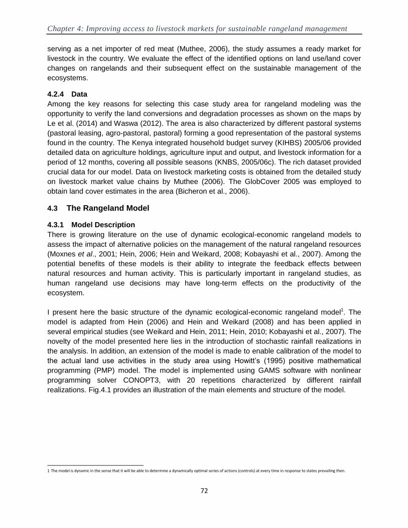
Chapter 4: Improving access to livestock markets for sustainable rangeland management
72
serving as a net importer of red meat (Muthee, 2006), the study assumes a ready market for
livestock in the country. We evaluate the effect of the identified options on land use/land cover
changes on rangelands and their subsequent effect on the sustainable management of the
ecosystems.
4.2.4 Data
Among the key reasons for selecting this case study area for rangeland modeling was the
opportunity to verify the land conversions and degradation processes as shown on the maps by
Le et al. (2014) and Waswa (2012). The area is also characterized by different pastoral systems
(pastoral leasing, agro-pastoral, pastoral) forming a good representation of the pastoral systems
found in the country. The Kenya integrated household budget survey (KIHBS) 2005/06 provided
detailed data on agriculture holdings, agriculture input and output, and livestock information for a
period of 12 months, covering all possible seasons (KNBS, 2005/06c). The rich dataset provided
crucial data for our model. Data on livestock marketing costs is obtained from the detailed study
on livestock market value chains by Muthee (2006). The GlobCover 2005 was employed to
obtain land cover estimates in the area (Bicheron et al., 2006).
4.3 The Rangeland Model
4.3.1 Model Description
There is growing literature on the use of dynamic ecological-economic rangeland models to
assess the impact of alternative policies on the management of the natural rangeland resources
(Moxnes et al., 2001; Hein, 2006; Hein and Weikard, 2008; Kobayashi et al., 2007). Among the
potential benefits of these models is their ability to integrate the feedback effects between
natural resources and human activity. This is particularly important in rangeland studies, as
human rangeland use decisions may have long-term effects on the productivity of the
ecosystem.
I present here the basic structure of the dynamic ecological-economic rangeland model1. The
model is adapted from Hein (2006) and Hein and Weikard (2008) and has been applied in
several empirical studies (see Weikard and Hein, 2011; Hein, 2010; Kobayashi et al., 2007). The
novelty of the model presented here lies in the introduction of stochastic rainfall realizations in
the analysis. In addition, an extension of the model is made to enable calibration of the model to
the actual land use activities in the study area using Howitt‘s (1995) positive mathematical
programming (PMP) model. The model is implemented using GAMS software with nonlinear
programming solver CONOPT3, with 20 repetitions characterized by different rainfall
realizations. Fig.4.1 provides an illustration of the main elements and structure of the model.
1 The model is dynamic in the sense that it will be able to determine a dynamically optimal series of actions (controls) at every time in response to states prevailing then.

Chapter 4: Improving access to livestock markets for sustainable rangeland management
73
Source: Adapted from Hein (2010) with modifications by the author
4.3.2 Optimization Problem
Households are assumed to maximize the sum of gross margin per hectare across all hectares
subject to production constraints. In the study area context, there are five main possible
production activities: four different crops (wheat, maize, beans, and potatoes) and grass,
representing pasture areas. The optimal combination of production activities is solved using the
PMP approach with a nonlinear land cost function 1(Mérel and Howitt, 2014; Howitt, 1995).
For wheat, maize, beans, potatoes, and grass; the optimization problem is defined as:
s.t . (4.2)
1 Heterogeneous land quality results in the marginal cost per unit of output increasing as more land is converted to croplands.
i
i
n
j
ijjiiiiii
i
i lawlllypMax
2
)5.0(
bAx
Figure 4.1: Main components of the ecological-economic rangeland model
Optimization Process
-Determine optimal combination of production
activities
-Households maximize the sum of gross margin per
hectare across all hectares
-PMP model is employed
Market Opportunities
Livestock
Production
Stochastic
Rainfall Grass Production
Land Allocation Decisions
Land allocated to
crop production
ANPP, kg DM/ha
Grazing
Intensities
Land allocated to
livestock production
(range areas)
production
Crop Incomes Livestock Incomes
Optimal Stocking
Densities
-Determines a
dynamically optimal
series of actions at
every time t in response
to the state
-the control variable
(TLUs sold at time t)
and the state variable
(size of the livestock
herd

Chapter 4: Improving access to livestock markets for sustainable rangeland management
74
where is a matrix of technical coefficients of resource requirements, is the land allocated to
the crop which yields , and are respectively the intercept and slope of the cost function
per unit land, is the cost per unit of the input, A is a matrix with elements , and b is a
vector of resource constraints. Land is the binding constraint for calibration. Observed data is
used to calibrate the model to replicate initial land allocation conditions.
4.3.3 Crop production
The study adopts a constant elasticity of substitution (CES) production function for each crop.
The production function allows for substitution between production inputs1. Constant returns to
scale (CRS) regarding CES production function is assumed for Narok County. The parameters
of the CES are solved following Howitt (2005). Crop yields are assumed to be fixed2 while the
prices are exogenous. The output of crops is determined by the number of acres of land
allocated to each crop.
4.3.4 Rangeland Productivity/Degradation Assessment
Prolonged grazing pressures, with loss of grazing areas, leads to poor protective cover of the
soils. This increases the vulnerability of soils to degradation. Reduced vegetation cover coupled
with intense animal tracks from trampling exposes the grazing areas to soil erosion, among other
forms of degradation. Soil erosion leads to the loss of nutrient rich topsoil and exposure of
vegetation roots, thus affecting the productivity of the soils. The above process informs the
choice of the study‘s indicator of rangeland degradation/productivity as aboveground net primary
production (ANPP).
ANPP, or its quotient to the corresponding precipitation, rainfall use efficiency (RUE), are two
ecological parameters commonly used for assessing the rangeland ecosystem state (Le
Houérou 1988; Hein, 2006; Hein and de Ridder, 2006; Hein and Weikard, 2008; Ruppert et al.,
2012; Snyman and Fouché 1991). The principal ability of ANPP to assess an ecosystem‘s state
(including degradation and desertification) has been widely confirmed (Bai and Dent, 2006; Sala
et al., 1988; Snyman and Fouché, 1991; Prince et al., 1998; Diouf and Lambin, 2001; Holm et
al., 2003; Buis et al., 2009; Ruppert et al., 2012).
Studies on the relationship between grazing biomass and rainfall in ASALs in East Africa
demonstrate biomass production to be a linear function of rainfall (De Leeuw and Nyambaka,
1988; De Leeuw et al., 1991). Sites used to measure the relationships were either protected or
located in low grazing areas (De Leeuw and Nyambaka, 1988). To model biomass productivity,
the study adopts from the work of De Leeuw et al. (1991) the linear relationship between median
rainfall and annual aboveground net primary productivity (ANPP, kg DM/ha). The relationship is
measured in a neighboring region with similar characteristics as the study area.
1 With a lack of substitution elasticity available from existing studies and lack of data to estimate, the study fixes the CES value equal to 0.6 for all inputs. This allows for limited
substitution between the production inputs as observed from farmer production practices.
2 The focus of the model is on health of grazing areas (represented by area covered by grass).
ija il
iy i i
jwthj ija

Chapter 4: Improving access to livestock markets for sustainable rangeland management
75
Following Hein (2010) and Hein and Weikard (2008), the model in this study is formulated to
account for the feedback effects of grazing intensities on biomass production, where grazing
limits biomass growth and the marginal reduction increases with high stocking rates (Hein and
Weikard, 2008). The model also incorporates the effects of uncertain rainfall events on biomass
production. In semi-arid areas, rainfall occurrence is primarily bimodal with two distinct rainy
seasons: short rains (October to December) and the long rains (March to May) (Biamah, 2005).
Four possible rainfall realizations for each season (very low, low, fair, and high) are considered.
A time series of stochastic rainfall realizations is obtained from scenarios of possible
combinations of short and long rains, together with the probability of their realization. Land users
make decisions ex ante in view of the risks and encounter the ‗realized‘ stochastic value of
rainfall ex post (Domptail and Nuppenau, 2010).
4.3.5 Available Forage
Unlike the high-potential areas, pastures are the main source of livestock feed in ASALs. About
90% of the livestock diet in rangelands is composed of natural pastures 1 . Crop residues
constitute negligible components of livestock feed, while fodder crops are hardly grown in the
dry lands. Total available livestock forage in the model is formulated as being governed by
biomass productivity by hectare (ANPP, kg DM/ha) and pasture/grazing area. A 'proper-use
factor' forage allowance is made where the standard 50% (or ―take half, leave half‖) rule of
thumb in range management is employed. An adjustment factor for biomass share available for
livestock use is also made as some of the biomass produced is consumed by other herbivorous
animals among other uses.
4.3.6 Optimal Stocking Levels
Livestock producers‘ current decisions do have an effect on the long-term productivity of
rangelands. Successful decisions should therefore constitute an optimal sequence of actions
based on the level of state variables in each period. This is achieved by adopting the value
iteration approach that solves the Bellman equation (Judd, 1999; Howitt 2005; Kobayashi et al.,
2007). The livestock producer‘s problem is presented as follows:
);x(xx| 1t
0
0 tttt
t
tc
gccfEMax (4.3)
where tx is the state variable (the size of the livestock herd measured in Tropical Livestock
Units) tc is the control variable (TLUs sold at time t), .0E is the expectation operator, .f is
the current profit equation; is the discount factor; ).(g characterizes net livestock herd size
1 Statement made from field observations as well as calculations from the 2005/06 KNBS survey

Chapter 4: Improving access to livestock markets for sustainable rangeland management
76
expansion. It also constitutes the equation of motion1; and t is the level of stochastic forage
production2.
Equation (4.3) presents an infinite-horizon problem where livestock producers aim at maximizing
the current and future profits. As stated earlier, current decisions do have an impact on the long-
term productivity of the ecosystems. Optimal livestock producers would therefore consider the
state of forage production in each time period when making decisions. A closed-loop system is
therefore defined where feedback occurs from information obtained on the level of state
variables in each time period (Kobayashi et al., 2007).
The livestock producer‘s problem is then presented using the Bellman equation as follows:
);(; 111 ttt
ctt xVEcfMaxxV
tt
(4.4)
where .V is the value function and .1t
E represents the expectations formed on forage
production in period 1t . The Bellman equation expresses the value function as a combination
of a current payoff and a discounted continuation payoff. The forward solution of the equation is
such that the sum of the maximized current payoff and the discounted or carry-over value
maximize the total value function (Howitt 2005).
The livestock sale control is represented as follows:
1
~
;
ttttt xxgxc (4.5)
where ~
t is the realized forage production.
Using equation (4.5), the control variable ( tc ) can be expressed in terms of the optimal herd
size in the next period ( 1tx ) (Kobayashi et al., 2007). Equation (4.4) can then be rewritten as:
);());((; 111
~~
11
ttttttx
tt xVExxgxfMaxxVt
t
(4.6)
Rewriting equation (4.6) using (.) and substituting the next period's value function gives:
});();,({);,(; 22121
~
1
~
12
11
tttttx
tttx
tt xVExxMaxExxMaxxVt
tt
t
(4.7)
The first order condition of equation (4.7) (w.r.t. 1tx in time t ) gives us the Euler condition:
1 We can logically assume that (.)g is concave in x i.e. 0' xg , 0'' xg
2 Because future rainfall events are unknown, the model incorporates uncertainty with the help of probability
distribution.

Chapter 4: Improving access to livestock markets for sustainable rangeland management
77
1
121
1
~
1 );,();,(
t
ttt
t
ttt
x
xx
x
xx
(4.8)
Equation (4.8) defines the condition for intertemporal optimality (Kobayashi et al., 2007). The
left-hand side gives the marginal cost, where the marginal cost is measured by potential
marginal payoffs foregone in period t, while the right-hand side gives the discounted marginal
payoffs in period 1t .
Following Judd (1999), Howitt (2005) and Kobayashi, et al. (2007), the study employs a
Chebychev Polynomial to obtain a continuous approximation to the value function. The
approximation is given as:
)()( xVxV
^
1
xj
n
j
j (4.9)
Where j is the coefficient of the thj polynomial term (.)j and
^
x is the state variable mapped
onto [–1, 1] interval on which Chebychev polynomial functions are defined.
4.3.7 Herd Dynamics
Following Hein (2010), to model livestock dynamics, the livestock herd is assumed to follow a
logistic growth process:
tttt xMTLUxLAMx *))/(1(* (4.10)
where tx are the tropical livestock units (TLU) 1 in the current period, tx is the change in TLU,
captures the potential natural growth in livestock, and is the maximum grazing
capacity of the grazing areas.
Livestock in the next period ( 1tx ) are determined by the livestock growth process defined in Eq.
(4.10) above and the number of sales ( tc ) as shown below:
tttttt cxMTLUxLAMxx )*))/(1(*(1 (4.11)
Livestock sales are considered to be the key source of livestock production revenue in the
grazing areas. The prices/costs incorporated in the model are assumed to be deterministic. The
detailed model is presented in the appendices (see Appendices B-D).
1 1 TLU = 1.43 cattle or
10 sheep or goats
LAMtMTLU
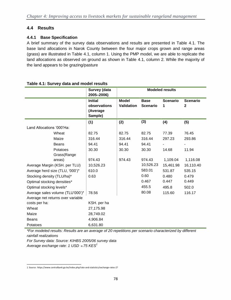
Chapter 4: Improving access to livestock markets for sustainable rangeland management
78
4.4 Results
4.4.1 Base Specification
A brief summary of the survey data observations and results are presented in Table 4.1. The
base land allocations in Narok County between the four major crops grown and range areas
(grass) are illustrated in Table 4.1, column 1. Using the PMP model, we are able to replicate the
land allocations as observed on ground as shown in Table 4.1, column 2. While the majority of
the land appears to be grazing/pasture
Table 4.1: Survey data and model results
Survey (data
2005–2006)
Modeled results
Initial
observations
(Average
Sample)
Model
Validation
Base
Scenario
Scenario
1
Scenario
2
(1) (2) (3) (4) (5)
Land Allocations ‗000‘Ha:
Wheat 82.75 82.75 82.75 77.39 76.45
Maize 316.44 316.44 316.44 297.23 293.86
Beans 94.41 94.41 94.41 - -
Potatoes 30.30 30.30 30.30 14.68 11.94
Grass(Range
areas) 974.43 974.43 974.43 1,109.04 1,116.08
Average Margin (KSH. per TLU) 10,526.23 10,526.23 15,461.98 16,110.40
Average herd size (TLU, ‗000‘)* 610.0 583.01 531.87 535.15
Stocking density (TLU/ha)* 0.63 0.60 0.480 0.479
Optimal stocking densities* 0.467 0.447 0.449
Optimal stocking levels* 455.5 495.8 502.0
Average sales volume (TLU‗000‘)* 78.56 80.08 115.60 116.17
Average net returns over variable
costs per ha:
KSH. per ha
Wheat 27,175.98
Maize 28,749.02
Beans 4,906.84
Potatoes 6,631.80
*For modeled results: Results are an average of 20 repetitions per scenario characterized by different
rainfall realizations
For Survey data: Source: KIHBS 2005/06 survey data
Average exchange rate: 1 USD 75 KES1
1 Source:
https://www.centralbank.go.ke/index.php/rate-and-statistics/exchange-rates-2?
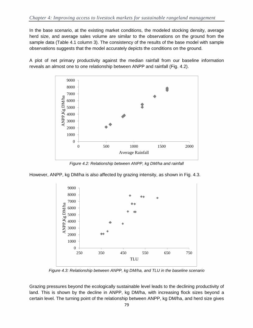
Chapter 4: Improving access to livestock markets for sustainable rangeland management
79
In the base scenario, at the existing market conditions, the modeled stocking density, average
herd size, and average sales volume are similar to the observations on the ground from the
sample data (Table 4.1 column 3). The consistency of the results of the base model with sample
observations suggests that the model accurately depicts the conditions on the ground.
A plot of net primary productivity against the median rainfall from our baseline information
reveals an almost one to one relationship between ANPP and rainfall (Fig. 4.2).
Figure 4.2: Relationship between ANPP, kg DM/ha and rainfall
However, ANPP, kg DM/ha is also affected by grazing intensity, as shown in Fig. 4.3.
Figure 4.3: Relationship between ANPP, kg DM/ha, and TLU in the baseline scenario
Grazing pressures beyond the ecologically sustainable level leads to the declining productivity of
land. This is shown by the decline in ANPP, kg DM/ha, with increasing flock sizes beyond a
certain level. The turning point of the relationship between ANPP, kg DM/ha, and herd size gives
0
1000
2000
3000
4000
5000
6000
7000
8000
9000
0 500 1000 1500 2000
AN
PP
,Kg
DM
/ha
Average Rainfall
0
1000
2000
3000
4000
5000
6000
7000
8000
9000
250 350 450 550 650 750
AN
PP
,Kg D
M/h
a
TLU

Chapter 4: Improving access to livestock markets for sustainable rangeland management
80
us the optimal stocking density, beyond which increasing grazing intensities will have a negative
effect on the ecosystems. At the base level, the optimal herd size of 455.5 TLU yields an optimal
stocking rate of 0.47 TLU/ha, which is significantly below the observed current stocking rates of
0.63 TLU/ha and the modeled 0.60 TLU/ha (Table 4.1). The results indicate that the current
grazing-livestock population exceeds the total grazing capacity in the area.
4.4.2 Re-apportioning value-added in the livestock marketing chain
: Incorporating livestock producers directly into the value-addition chain and
linking them to existing terminal livestock: Scenario 1
The detailed study on livestock market value chains in the country by Muthee (2006) is used to
estimate changes in producers‘ benefits from incorporating livestock producers directly into the
value-addition chain and linking them with the buyers at the terminal market. The above concept
has been employed, on a small scale, by organizations such as CARE Kenya1, thus ensuring its
practicability. The approach involves establishing a market-based intervention whereby the
pastoralists are organized into producer associations and enabled to participate in the value-
addition chain (fattening of animals before sale) and linked to the livestock terminal markets
(McKague et al., 2009; Muthee, 2006). Strengthening vertical linkages between fattening camps
and livestock producers improves the live weight of livestock, enabling the producers to receive
better margins, unlike in cases in which livestock is sold to middle men at the primary markets.
On the other hand, linking livestock producers to existing terminal markets would minimize the
exploitation by middlemen and further improve the livestock producers‘ margins.
The purpose of organizing producers into groups is to improve cooperation among pastoralists,
reduce transport costs and consolidate supply, and improve the collective bargaining power of
the livestock producers (McKague et al., 2009). As in the case of CARE Kenya, existing
producer associations, such as water users associations commonly found in pastoral and agro-
pastoral areas, can be used as a basis of these producer-marketing groups. The use of existing
groups limits the transaction costs of forming new associations. From the above, this study is
based on the assumption that there are existing producer associations which would act as the
basis of the above market base intervention. Hence, no transaction costs associated with
forming new associations are incurred.
This market-based intervention also requires the help of a value chain actor/market facilitator,
whereby the role can be played by either the government, or, as in the case of CARE Kenya, by
an NGO. The work of the value chain actor is just to provide support, meaning they are not
involved in buying or selling but mainly assist in removing obstacles that limit livestock producers
from participating in the terminal markets (McKague et al., 2009). The related costs of the
intervention, such as the transport costs to the terminal markets and the costs of facilitating
contracts at the terminal markets, fattening fees at fattening camps, among other costs, are
provided in detail in the study by Muthee (2006) (Table 4.2). It is on the basis of the existing
1 A non
-governmental organization involved in creating market linkages to livestock farmers by enabling them to become involved in the value chain itself charging a small fee for
operational costs
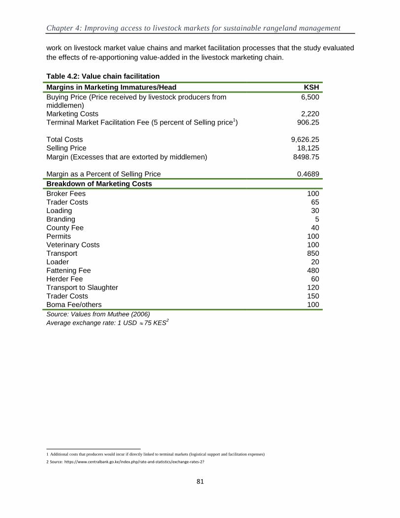
Chapter 4: Improving access to livestock markets for sustainable rangeland management
81
work on livestock market value chains and market facilitation processes that the study evaluated
the effects of re-apportioning value-added in the livestock marketing chain.
Table 4.2: Value chain facilitation
Margins in Marketing Immatures/Head KSH
Buying Price (Price received by livestock producers from middlemen)
6,500
Marketing Costs 2,220
Terminal Market Facilitation Fee (5 percent of Selling price1) 906.25
Total Costs 9,626.25
Selling Price 18,125
Margin (Excesses that are extorted by middlemen) 8498.75
Margin as a Percent of Selling Price 0.4689
Breakdown of Marketing Costs
Broker Fees 100
Trader Costs 65
Loading 30
Branding 5
County Fee 40
Permits 100
Veterinary Costs 100
Transport 850
Loader 20
Fattening Fee 480
Herder Fee 60
Transport to Slaughter 120
Trader Costs 150
Boma Fee/others 100
Source: Values from Muthee (2006)
Average exchange rate: 1 USD 75 KES2
1 Additional costs that producers would incur if directly linked to terminal markets (logistical support and facilitation expenses)
2 Source:
https://www.centralbank.go.ke/index.php/rate-and-statistics/exchange-rates-2?

Chapter 4: Improving access to livestock markets for sustainable rangeland management
82
Linking livestock producers to the end
market and involving them in the livestock
value addition is estimated to increase the
producers‘ margin by 46.89% (Table 4.2).
With the increased benefits associated with
livestock production, land allocation moves
in favor of livestock production (grass).
Higher producer margins lead to land
allocated for livestock production
increasing from 974,431ha to 1,109,041ha,
confirming that land allocations are driven
by the benefits the land users expect to
derive from the land (Table 4.1, column 4).
The reallocated land is crucial as it
represents the regaining part of former
fertile rangelands. Higher allocation of land
for grazing purposes is likely to facilitate
livestock mobility and access to wider
pasture areas. We further evaluate the
effect of increased land allocation to land
management and livelihoods (Fig 4.4).
With the re-apportioning of value addition
and links to terminal markets, we observe
the increased livestock sales levels
compared to the base average sales level
(Table 4.1, column 4 and Fig. 4.4, a). With
livestock sales as the control variable in the
dynamic livestock model, increased
livestock sales indicate that livestock
producers are able to utilize markets more
in taking action (livestock sales) in every
time period in response to the state of the
rangelands. This leads to better
management of land as productivity
increases and is less variable compared to
the base scenario (Fig. 4.4, c). In addition,
compared to the optimal stocking density of
0.45 TLU/ha1 in Scenario 1, the stocking
density of 0.48 TLU/ha indicates better
management of land, given its close proximity to the optimal level and also compared to the
Base Scenario stocking density of 0.60 TLU/ha (Table 4.1, column 4).
1 Obtained at the turning point of the relationship between ANPP, kg DM/ha and herd size as shown in Fig. 4.3
Figure 4.4: Plots of model output results. The results are
an average of 20 repetitions per scenario characterized by
different rainfall realizations. Legend: 1=Baseline
Scenario; 2=Scenario1; 3=Scenario 2.
a
b
c
Chapter 4: Improving access to livestock markets for sustainable rangeland management
83
Given the higher off-take levels, as expected, the herd size in Scenario 1 is lower compared to
that of the base scenario (Table 4.1, column 4 and Fig. 4.4, b). While this might not look
appealing at first sight; Scenario 1 presents a better strategy, as it involves fewer variations in
herd sizes. With livestock as important assets for pastoralists, Scenario 1 presents more stable
wealth levels for the livestock producers (Fig. 4.4, b). In addition, fewer variations in livestock
levels indicate that the producers are less likely to face drastic reductions in livestock compared
to the base scenario. The live weight of livestock is also expected to be better in Scenario 1,
given the higher productivity levels compared to the base scenario.
4.4.3 Efficient livestock transportation means
: Efficient livestock transportation means in addition to re-apportioning value-
added in the livestock marketing chain: Scenario 2
Similarly to the value addition and terminal market scenario, all the transports costs (trucking of
livestock) were obtained from the detailed livestock market study by Muthee (2006). Transport
costs constitute a large share of livestock marketing costs in the country, going as high as 65%
of the total marketing costs in some parts of the country (Muthee, 2006). In Narok,
trucking/trekking costs constitute about 40% of the total marketing cost (Muthee, 2006). Trucking
vehicles are normally hired and the associated costs charged per livestock head (transport,
loading, and off-loading). With the aim of mitigating the high transportation costs, the study
evaluates the effects of adopting efficient transportation means at the prevailing road
infrastructure conditions. The use of a double-decker trailer as a transport means is assessed as
a possible means of reducing transportation costs. A standard double-decker transporter has the
capacity to carry 26 cattle and 70 shoats (Muthee, 2006). We assess the benefits/savings made
by transporting shoats alongside cattle in a double-decker cabin versus transporting the shoats
separately (see table in Appendix C).
Use of a double-decker truck increases the producers‘ margin further by 6.16%, leading to land
allocations as shown in Table 4.1. Higher producer margins have the potential of increasing land
allocated to pastures to 1,116,076 ha (Table 4.1).
Similar to Scenario 1, the higher producer margins with the use of a double-decker truck are
associated with higher livestock sales levels compared to the base average sales level (Table
4.1, column 5 and Fig. 4.4, a). This indicates the use of efficient transport not only facilitates
movement of livestock to the terminal markets but also that producers are able to save on
transportation costs. As highlighted earlier, increased sales levels indicate the ability of livestock
producers to utilize livestock markets more in taking action (livestock sales) in response to the
state of the rangelands. With higher ability to take action in response to the state of the land,
productivity of the rangelands increases and is less variable compared to the base scenario and
Scenario 1 (Fig. 4.4, c). Similar to Scenario 1, the optimal stocking density in Scenario 2 is given
as 0.45 TLU/ha1. The stocking density of 0.475 TLU/ha indicates better management of land
compared to the Base Scenario and Scenario 1 (Table 4.1, column 5)
1 Obtained at the turning point of the relationship between ANPP, kg DM/ha and herd size as shown in Fig. 4.3
Chapter 4: Improving access to livestock markets for sustainable rangeland management
84
Increased participation in livestock markets leads to lower livestock levels in Scenario 2
compared to the Base Scenario but higher compared to Scenario 1 due to more land allocations
for grazing purposes (Table 4.1, column 5, and Fig. 4.4, b). Scenario 2 is also associated with
higher and more stable wealth levels compared to Scenario 1 and the base level. This is from
the higher herd sizes compared to Scenario 1 and stable livestock levels compared to the Base
Scenario (Fig. 4, b).
4.5 Discussion and policy Implications
Competing land use options in rangelands are likely to lead to the conversion of grazing
vegetation to other land uses/land covers with subsequent consequences on the health of the
ecosystems. The increasing practice of crop cultivation on the rangelands is identified as a
serious threat to future livestock production and rangeland management (Solomon et al., 2007).
Expansion of crop farming curtails the traditional adaptive strategies of pastoralists and limits the
mobility of livestock and access to key resources in particular during dry seasons (Butt, 2010).
This leads to concentrated livestock densities above optimal levels on the rest of the rangeland,
as shown in the initial observations (Table 4.1). The key consequence of rangeland losses is
restricted access and mobility of livestock (Flintan, 2011), leading to high livestock densities and
unsustainable production on the rest of the rangeland. This is demonstrated by the effect of
large herd sizes on the productivity of rangeland (ANPP,Kg DM/ha) beyond the optimal level
(Fig. 4.4, c).
Indeed, while crop farming may provide an alternative to pastoralism, especially in the wetter
semi-arid areas, the associated costs, in the mid- to long term, appear too great to bear (Davies
and Bennett, 2007). With lower productivity of the grazing areas (ANPP, kg DM/ha) and high
livestock densities (0.6 TLU/ha), communal pastoralists become more vulnerable to the
ecological climate variability of rangelands resulting in larger livelihood impacts (Fig. 4.4, b). This
is in line with observations of Banks (2003), stating that the opportunity costs of disrupting the
traditional operations of rangelands are overlooked, while the benefits may be overstated.
Among the overlooked costs are the effects of rangeland use changes on biological diversity
and the ability of biological systems to support human needs (Maitima et al., 2009). The effect of
the loss of rangelands on the sustainability of the ecosystems is further exacerbated by low take-
off rates of livestock. Well-established markets could greatly facilitate the movement of livestock
from areas of forage scarcity, thereby regulating livestock densities and minimizing the
ecological vulnerabilities of the dry lands (Turner and Williams 2002).
To understand the driving forces of the observed transformations in rangelands, emerging now
is the acknowledgement of the presence and interaction of both equilibrium and non-equilibrium
factors in the dynamics and the paths of rangeland degradation (Vetter, 2005; Domptail, 2011).
Responses to emerging economic opportunities, facilitated by institutional factors, are driving the
observed rangeland uses (Lambin et al., 2001). Rangeland users in the region, as with other
developing countries, no longer live outside the cash economy (Davies and Bennett, 2007).
Expected economic gains have been observed to influence their land use decisions. This is
shown by the land allocation decisions in response to changes in returns realized from the
current land uses. For instance, Table 4.1 shows how land allocations to various land uses differ
from the base land allocations in response to the increased benefits associated with livestock

Chapter 4: Improving access to livestock markets for sustainable rangeland management
85
production. The reverse, as has been the case, can also occur as shown by Tiffen et al. (1994),
where expansion of the area under cultivation occurs in a semi-arid area with increased crops
marketing opportunities and a decrease in livestock prices.
In their study, Tiffen et al. (1994) show that the progress of rural farmers can be facilitated by
raising producers‘ prices through transport improvements and minimization of marketing costs.
However, livestock markets function poorly with high marketing costs and high reliance on
itinerant traders with whom they often have poor bargaining power to sell stock; this finding
corroborates with that of McDermott et al. (2010), Makokha et al. (2013), and Muthee, (2006).
The inefficiencies characterizing the livestock markets affect the benefits that livestock
producers receive and drive rangeland use changes where opportunities prevail.
In addition to sustaining livelihoods, improved livestock marketing may have significant
opportunities for improving environmental management (Frost et al., 2007). Ecological research
shows that, with erratic rainfall characterizing rangelands in ASALs, the design of marketing
systems should be such that they absorb fluctuations in marketed livestock. Among the
components of such marketing systems identified is access to the largest markets and improved
transport infrastructure (Behnke, and Kerven, 1994). Similar to Turner and Williams (2002), we
found that livestock markets are capable of facilitating the destocking of animals leading to
better productivity of land (Table 4.1; Fig. 4.4). Improving market access through the creation of
opportunities for pastoralists to sell livestock more profitably and lower transportation costs
increases the benefits associated with rangelands, leading to higher land allocations to grazing
purposes (Table 4.1). Our analysis concurs with previous empirical work by Barrett and Luseno
(2004), highlighting the main factors affecting livestock producers‘ earnings in the country as
transportation costs and lack of competition within the marketing channel which create an
unattractive marketing environment for pastoralists. Price fluctuations in the terminal market
provide little empirical justification to worry about (Barrett and Luseno, 2004). Improved earnings
associated with range areas are also observed to stabilize wealth of households (Fig. 4.4 c).
This is expected to have direct positive effects on the livelihoods of rural rangeland users and
less vulnerability to the variable ecological climate characterizing ASALs.
Currently, the existing national policy for the sustainable development on ASALs, titled,
―Releasing our full potential,‖ entails a key number of objectives aimed at achieving the
sustainable use of rangelands while improving livelihoods. Among the elements include 1) the
development of an enabling environment for accelerated investment in foundations to reduce
poverty and build resilience and growth; 2) a responsive government to the uniqueness of arid
lands which include ecology, mobility, population distribution, economy, and social systems; and
3) climatic resilience (GOK, 2012a). Our findings could prove useful if brought into play by
Kenyan ASALs policy planners. The findings suggest that policy measures to attain the stated
objectives should include efforts to minimize barriers limiting livestock producers‘ participation in
value-added livestock production and access to high-value markets such as terminal markets.
This can be achieved, as illustrated in the study, by minimizing/eliminating the price market
disincentives currently characterizing rangelands. Second, community participatory approaches,
such as producer groups, could be used as market-based interventions for livestock producers.
Policy action promoting collective action at the grass-roots levels is therefore likely to have

Chapter 4: Improving access to livestock markets for sustainable rangeland management
86
positive effects not only on improving livelihoods but also on the sustainable management of
rangelands.
The study acknowledges that additional policies should go hand in hand with efforts to make
livestock markets serve as mechanisms of destocking livestock, especially during periods of low
biomass production as well as promote sustainable rangeland management. Although
pastoralists have been shown to be generally open minded, capable of producing livestock
optimally (Kimani and Pickard, 1998; Mwangi and Meinzen-Dick, 2009), and in great need for
stronger links to the outside world, such as with improved livestock market access (Coppock,
1994), more incentives may be required for active participation in markets and sustainable
rangeland management practices. An existing initiative that would complement the improved
access to livestock markets would be the expansion of the index-based livestock insurance
(IBLI). Insurance of livestock would be a critical concept encouraging livestock producers to
participate in livestock markets. Insurance would enable the producers to stabilize their livestock
accumulation, making them less likely to face drastic reductions in livestock, with increased
offtake levels, in the event of a shock from the risky climatic conditions characterizing range
areas. In addition, improved access to livestock markets coupled with IBLI is likely to lead to
crowding in of finance to provide the much-needed credit for the economic development of the
rangelands.
In addition, the livestock production associations can further be used to foster cooperation
among pastoralists, for example, with regard to how much of the grazing areas should be
unaltered and also on livestock production strategies, such as stocking levels. Such cooperation
among pastoralists currently exists, as observed in the case of conservancies, where land use
regulations have contributed to numerous ecosystem benefits (Osano et al., 2013). Producer
associations therefore present a viable option to foster sustainable management practices in
semi-arid grazing lands as a complement to market-based interventions. Further research work
may address other possible synergies between improved livestock incomes and sustainable
rangeland management.
4.6 Conclusions
Livestock production plays a key role in the economic development and welfare of the county. In
spite of their significant role, rangelands in the country are being impaired by factors related to
LULCC. Among the key factors driving conversion of rangelands to other land use/land covers
are the changing opportunities brought about by markets. This study explores the linkages
between improved livestock market access, rangeland use change, and livestock producers‘
livelihoods in the semi-arid Narok County of Kenya. In an effort to realize potential economic
benefits with rising domestic and export markets for crops, fertile rangelands are observed to be
increasingly converted to crop farming in the country. Among the resulting consequences of the
declining range areas are degradation of rangeland ecosystems leading to negative effects on
the social and economic security of the remaining livestock producers.
This study shows that improved livestock market access affects the economic returns of
producers, which in turn affects rangeland management decisions. Improved market access in
the study is sought through the creation of opportunities for pastoralists to sell livestock more

Chapter 4: Improving access to livestock markets for sustainable rangeland management
87
profitably by re-apportioning value-added in the livestock marketing chain, linking them with
terminal markets and through reduced livestock transportation marketing costs. Livestock
producers‘ margins improve with re-apportioning value-added and reduced livestock marketing
costs. Increased benefits associated with livestock production, on the other hand, lead to fewer
conversions of former rangelands to crop farming, stabilizes herd levels, and increases market
participation among livestock producers. The livelihood of livestock producers improves with
better earnings and stabilized assets levels. In addition, livestock producers‘ vulnerability to
ecological climate variability characterizing rangelands is reduced with better productivity of the
ecosystems. From the study findings, national policy on improved livelihoods of pastoral
communities should therefore entail efforts to include pastoralists in value-added livestock
production and also access to high-value markets.

88
Chapter Five
5 Basic Capabilities Effect: Collective Management of
Pastoral Resources in South Western Kenya
5.1 Introduction
Co-management of pasture resources under collective ownership systems has gained
importance in managing and structuring the use of rangelands in arid and semi-arid areas
(Banks, 2003; Hundie and Padmanabhan, 2008; Mwangi and Meinzen-Dick, 2009; Ostrom,
1990). Under these systems of joint provision and exploitation of range resources, pastoralists
have access to diverse livelihood options to hedge against risks (Kimani and Pickard, 1998;
Mwangi and Meinzen-Dick, 2009). The risks mainly emanate from low and erratic rainfall and
variations in pasture productivity characterizing the arid and semi-arid lands (ASALs). With
regard to diverse livelihood options, communal ownership of rangeland resources allows users
to have access to a larger land area that provides water and pastures in both the dry and wet
seasons. This serves as an insurance against individuals incurring losses, especially during dry
periods (Mwangi and Meinzen-Dick, 2009). As further illustrated by the authors, collective rights
to land and land resources in range areas provide a more equitable way of distributing variable
resources and are associated with significant savings on transactions and production costs
(Mwangi and Meinzen-Dick, 2009). In addition, collective systems present the necessary scale
required to maintain the ecological function of the heterogeneous land surfaces associated with
rangelands (Baland and Platteau, 1996; Meinzen-Dick and Mwangi, 2009; Ostrom, 1990). The
system provides the scale necessary for mobility that supports more sustainable livestock
production in marginal environments (Mwangi, 2009).
Redefinition of traditional land use arrangements from communal ownership to exclusive
property rights has however been observed to result in fragmentation, a key cause of rangeland
degradation (Amman and Duraiappah, 2004; Flintan, 2011; Galaty and Ole Munei, 1999; Rutten,
1992). Fragmentation of rangelands results in the loss of flexibility of livestock movements. This
disrupts the seasonal movements of livestock necessary to access resources (water and
pastures) that are heterogeneous in space and time (Flintan, 2011). Restricted mobility of
livestock has been shown to lead to the loss of the opportunistic spread of grazing pressure and
ultimately leads to the overuse of resources in the confined areas (Boone and Hobbs, 2004;
Hobbs et al., 2008; Meinzen-Dick and Mwangi, 2009). Fragmentation also occurs with the loss of
land, especially in well-watered areas, to alternative land uses such as crop farming.
Chapter 5: Collective Management of Pastoral Resources in South Western Kenya
89
Well-watered areas (i.e., dry season grazing areas) provide grazing relief in the marginal areas
(wet season grazing areas), particularly during the dry seasons (Wade, 2013). Thus the loss of
well-watered areas subjects the marginal areas to serious environmental degradation through
depletion of biomass, loss of biodiversity, and soil erosion (Mireri et al., 2008; Mwagore, 2003).
This undermines the capacity of pastoral communities to sustainably use the ecosystems as well
as deal with risks such as droughts.
While the benefits of collective management of natural resources such as rangelands are clear,
what remains unclear are the conducive factors to successful collective actions. Collective
management of natural resources does not always emerge, and thus attention by a number of
studies on factors either facilitating or hindering participation in collective action emerges
(Agrawal, 2001; Dayton-Johnson, 2000; Gebremedhin et al., 2004; Meinzen-Dick et al., 2002;
Ostrom, 2009; Willy and Holm-Müller, 2013). While there has been some general consensus on
the role of certain factors, such as the number of users, importance of the resource system to
users, and mobility of the resource system (Agrawal, 2001; Baland and Platteau, 1999; Ostrom,
2009), the role of some factors is debatable. For instance, on one hand, social networks and
social participation, which are key elements of social capital, have been identified to enhance
individuals‘ interactions in societies and facilitate participation in collective action (Gebremedhin
et al., 2004; Willy and Holm-Müller, 2013). On the other hand, social capital may bring about
subjective norms and may affect collective action negatively (Ajzen and Fishbein, 1980). For
example, perceived social pressure to opt for subdivision of commonly managed pastures would
hinder the collective management of pastoral resources. Market orientation has also been found
to affect the capacity of communities to manage resources collectively. It has been found that, in
some market-integrated societies, cooperative behavior prevails. In these environments,
markets have been found to foster social interactions, leading to the evolution of norms that
influence individual values and returns to relationship-specific investments (Bowles, 1998).
However, markets may result in competitive environments undermining collective action
(Agrawal, 2001; Carpenter and Seki, 2005). The composition of resource users within a group is
also likely to affect collective actions in natural resource conservation. While some studies argue
that inequalities in wealth within a community facilitate collective action in overcoming social
dilemmas (Baland and Platteau, 1999, 2007; Naidu, 2009), others argue that inequalities may
lead to low levels of collective action and cooperation (Dayton-Johnson, 2000; Gebremedhin et
al., 2004; Janssen et al., 2011; Johnson and Smirnov, 2012).
The seemingly inconsistent results highlight the importance of the context in which collective
action occurs (Baland and Platteau, 2007). This paper aims at contributing to the literature on
factors affecting the collective management of natural resources. The study provides evidence
on the role of basic capabilities as a determinant of collective action in communal grazing land
management in a semi-arid setting. Capabilities, as defined by Krishnakumar and Ballon (2008),
refer to the ability to achieve and relate not only to the opportunities that individuals access but
to also the opportunities that one could potentially have access to (Ballet et al., 2015). Basic
capabilities, as defined by the UNDP (1997), refer to the opportunity to achieve some minimally
acceptable levels of functioning – the presence of some basic capabilities to function.
Functionings, on the other hand, refer to the various valuable things that an individual manages

Chapter 5: Collective Management of Pastoral Resources in South Western Kenya
90
to do or be, that is, the doings and beings of an individual (UNDP, 1997; Krishnakumar and
Ballon, 2008).
As illustrated by Sen (2009), the important components of human capabilities relate to the well-
being of individuals, the role of individuals in influencing economic production, and the role of
individuals in influencing social change. Although these components are not directly observable,
they do manifest themselves in observable functionalities (Krishnakumar and Ballon, 2008;
Bérenger and Verdier-Chouchane, 2007). Capability constraints curtail the ability of individuals
to utilize the opportunities available to them (Ballet et al., 2015; UNDP 1997). In the context of
rangeland resource management, the geographical nature of the ecosystems (arid and semi-
arid lands) narrows the range of opportunities that individuals have at their disposal to exploit the
ecosystem. However, individuals‘ basic capabilities further determine individuals‘ capacity to
exploit the pasture resources in more ways than one (grazing), and this leads them to make
certain choices. The indigenous people residing in Kenyan rangelands primarily rely on common
resource ownership systems of livestock production to sustain their livelihoods. The inhabitants,
however, have been observed to react to increased opportunities to promote their economic
well-being (Campbell et al., 2005, 2003). With increased opportunities that one can access with
the exclusive appropriation of the resource pie and ability to exploit them, an individual
cooperating in common resource ownership is likely to exit and opt to exploit the potential higher
benefits.
In Kenya, there has been a growing body of research on collective action among smallholder
farmers (Andersson and Gabrielsson, 2012; Fischer and Qaim, 2012; Kariuki and Place, 2005;
Narrod et al., 2009; Willy and Holm-Müller, 2013). However, only a few studies focus on
collective action in pastoral drylands (Mwangi, 2007, 2009), with even fewer empirical studies
existing (Nduma et al., 2001) and none illustrating the contribution of basic capabilities, an
important factor explaining cooperation (Ballet et al., 2015). The present study fills this important
gap in this field of research, not only in terms of identifying the causal relationship between
multiple factors and the collective management of pastoral resources but also in showing how
basic capabilities impact collective action. The crossing between basic capabilities, among other
factors, and participation in collective management of grazing lands is thus the subject of
analysis in this paper. The objective is modeled in two separate questions: Which factors affect
(1) participation in collective management of pastoral resources and (2) the extent of
participation? To achieve the stated objective, the paper applies fractional variate estimation
procedures to data collected in a household survey among randomly selected agro-pastoral
households in six different divisions in Narok County, in Kenya.
The rest of the study is structured as follows: In Section 2, I present the institutional
developments in natural resource management in the study area. Section 3 presents the
conceptual and theoretical frameworks in addition to the empirical model. Section 4 describes
the location of the study area and data collection methods. Section 5 presents regression
results, while Section 6 discusses the results. Lastly, Section 6 draws policy implications and
concludes the study.
Chapter 5: Collective Management of Pastoral Resources in South Western Kenya
91
5.2 Understanding Institutional Developments in Natural Resource Management
in Narok County
5.2.1 Background
Narok County is located on the southwestern part of the Rift Valley Province of Kenya. The
county, a semiarid region, lies between latitudes 34°45'E and 36°00'E and longitudes 0°45'S and
2°00'S, with annual precipitation ranging from 500 to 1,800 mm and local variations in
topography playing a major role in the distribution patterns (Ojwang et al., 2010). The county has
three districts covering an area of about 17,933.1 km2, with an estimated population of 850,920
according to the 2009 census, and a population density of 47 people/km2 (Republic of Kenya,
2010). Most of the region, especially the central part of the county, is characterized by harsh
ecological conditions, resulting in low productivity. Farming is only suitable along the borders
(Jaetzold et al., 2009). Livestock production remains the key component of agricultural
production in Narok South and the lower parts of Narok North, with pastures forming the main
feed for livestock. In addition to serving as a means of livelihood, livestock production plays a
crucial role in the pastoralists‘ traditional social setting as a sign of wealth (Kaimba et al., 2011).
The county supports one of the richest masses of large herbivores worldwide, including
migratory wildebeest and a host of associated grazers, browsers, and predators (Ojwang et al.,
2010).
In the county, as is the case with the rest of the country, the political economy context is closely
linked to the processes of transformations in the institutions governing land ownership and land
use (Amman and Duraiappah, 2004; Campbell et al., 2003; Mwangi, 2009). In the pre-colonial
era, the area was mainly home to the Maasai pastoralists who practiced nomadic pastoralism
characterised by movement of livestock within seasons in search of pastures, water, and
incidence of disease (Campbell et al., 2005; Kimani and Pickard, 1998). Livestock production
formed the basis of their economic livelihoods (Campbell et al., 2005; Mwangi, 2007; Nyariki et
al., 2009). The livestock production system was defined by individual ownership of livestock with
collective use and ownership of pasture and water (Kimani and Pickard, 1998; Mwangi, 2007).
The socio-spatial organizations of the pastoralists comprised the household (the basic unit), the
boma (a number of households in the same compound), the neighborhood (a cluster of bomas),
and the section (a group of neighborhoods in the same area) (Kimani and Pickard, 1998). The
sections provided enough wet- and dry-season pastures and water and were protected against
encroachment by other pastoralists and farmers. Movement of herds out of the section occurred
only in cases of extreme drought (Kimani and Pickard, 1998). At the time of the European
arrival, the indigenous land use systems were dismantled and replaced with exclusive private
land ownership systems (Amman and Duraiappah, 2004). The indigenous populations were
deprived of the best lands that served as important dry-season and drought retreat and were
restricted to the marginal lands (Amman and Duraiappah, 2004; Campbell et al., 2005, 2003;
Kimani and Pickard, 1998).
Land adjudication at independence in many instances followed similar processes as those seen
during colonialism. High-potential land was allocated to elites and prominent individuals, while
the majority of pastoralists settled on the drier savannah lowlands (Amman and Duraiappah,

Chapter 5: Collective Management of Pastoral Resources in South Western Kenya
92
2004; Campbell et al., 2005). Even where initial distributions involved high-potential land
allocation to the indigenous people, special groups and immigrant farmers from other parts of
the country bought out the land from poorer land owners and, in most cases, at very low prices
(Amman and Duraiappah, 2004; Kimani and Pickard, 1998). For instance, in Narok County, the
relatively fertile land was occupied by Kalenjin and Kikuyu immigrants as well as special groups
of wealthy and politically connected commercial farmers (Amman and Duraiappah, 2004).
5.2.2 Group ranches and Re-aggregating individualized parcels
Group ranches were initiated in 1968 by the government of Kenya (Kimani and Pickard, 1998;
Mwangi, 2007, 2009). A group ranch consists of land that is legally jointly owned by a group,
such as a tribe, clan, section, family, or other group of persons, and is managed by a committee
elected by the members (Kimani and Pickard, 1998; Mwangi, 2009). The elected committee
controlled the resource use, that is, it managed the grazing, water, and tillage (Mwangi, 2009).
The group ranches were anticipated to encourage the pastoralists to invest in range
improvement and reduce the stocking rates, encourage commercialized livestock production,
increase the Maasai's contribution to the national economy, and provide the indigenous people
with tenure security and guard against landlessness among pastoralists (Kimani and Pickard,
1998; Mwangi, 2009). The communities welcomed the concept of group ranches to secure their
land and avoid the risk of losing more land from encroachment by immigrant farmers (Kimani
and Pickard, 1998; Mwangi, 2009). Group ranches were created to enclose sufficient wet- and
dry-season pasture and resources (Campbell et al., 2005). However, movement in extreme
drought years beyond the ranch boundaries remained necessary, and thus the strict boundaries
were not feasible (Campbell et al., 2005; Kimani and Pickard, 1998).
There has been a growing trend of group ranch sub-division into individual holdings (Carpenter
and Seki, 2005; Kimani and Pickard, 1998; Mwangi, 2007, 2009; Nyariki et al., 2009). Among
the identified factors motivating subdivision of group ranches are the difficulties in enforcing
collective interests in resource allocation and the need to protecting individuals‘ land claims
against threats of inappropriate allocation of group land to unauthorized individuals by the
management committee (Campbell et al., 2005; Kimani and Pickard, 1998; Mwangi, 2007, 2009;
Nyariki et al., 2009). While subdivision may initially have been motivated by poor management
and difficulties in enforcing collective interests, research indicates that other factors have been
important in motivating the transformation (Campbell et al., 2005; Mwangi, 2007). Other than the
need to access capital markets and the pressures from the increasing number of individuals
entitled to a share in a fixed land resource, subdivision appears to be an expedient strategy to
exploit economic opportunities with altered land-holding systems (Campbell et al., 2005, 2003).
For instance, individuals are observed to be eager to exploit opportunities arising from market
liberalization and crop market development (Campbell et al., 2005).
Land subdivision in the area has resulted in fragmented rangelands and sales to mostly
immigrant farmers, a key cause of rangeland degradation (Amman and Duraiappah, 2004;
Flintan, 2011; Galaty and Ole Munei, 1999; Kimani and Pickard, 1998; Rutten, 1992). Average
parcel sizes have decreased, while the number of fenced parcels and fragments converted to
other land uses, such as crop farming, has increased. Fragmented rangelands result in the loss
of flexibility and mobility of livestock. In addition, subdivision reduces the grazing capacity of land

Chapter 5: Collective Management of Pastoral Resources in South Western Kenya
93
and spread in opportunistic grazing, leading to the overuse of resources in the confined areas
(Boone and Hobbs, 2004; Hobbs et al., 2008; Meinzen-Dick and Mwangi, 2009). Furthermore,
due to subdivision, the indigenous people are losing the fertile lands and being pushed into the
marginal areas (Amman and Duraiappah, 2004; Kimani and Pickard, 1998). Exclusion further
exacerbates the processes of environmental degradation, as marginal lands are used intensively
beyond their capacity (Amman and Duraiappah, 2004; Kimani and Pickard, 1998). Ultimately,
the combined processes of fragmentation, exclusion, and inhibition lead to increasing levels of
poverty, both absolute and relative poverty (Amman and Duraiappah, 2004). It is, however,
worth noting that there are some group ranches that have resisted subdivision to date (Mwangi,
2007).
Besides the group ranches that have resisted subdivision, an interesting development in the
area has been the regrouping of some individual land owners in the area, with friends,
neighbours, or kin to pursue joint herd/pasture management in their re-aggregated parcels
(Mwangi, 2007). While each individual title holder retains the right to alienate his resource, the
regrouping allows access rights to resources, such as pastures, among single-titled owners who
have agreed to pursue shared strategies. Livestock benefit from rotational grazing in the shared
space given the radical changes in production systems. Aggregation of the individual parcels
indicates attempts to enhance sustainability of the production system given variation in the
environmental conditions and pasture productivity characterizing the areas (Mwangi, 2007).
Because dynamics in the land-holding systems involves rearrangement of use rights with
significant effects on sustainable land management, factors behind these changes are of
fundamental concern.
5.3 Frameworks
5.3.1 Conceptual Framework
The conceptual framework for this study is based on the theory of collective action (Ostrom,
1990, 2001, 2009), institutional economics (Kirsten et al., 2009a; Meinzen-Dick and Mwangi,
2009), and the capability approach by Sen (1980). In common property resources, rights are
held by a defined group. The rights refer to 1) access rights (the right to enter a defined
property), 2) withdrawal rights (rights to obtain goods from a resource, 3) management rights
(rights to transform the resource and control its use patterns, 4) exclusion rights (rights
preventing others to access the resource), and 5) alienation rights (rights to sell or lease or both
of the above mentioned rights) (Schlager and Ostrom, 1992; Mwangi and Meinzen-Dick, 2009).
These rights can be categorized as use rights and control or decision-making rights (Mwangi
and Meinzen-Dick, 2009). The decision whether to cooperate in the joint provision and
appropriation of pastoral resources or opt for an exclusive share of the resource pie would alter
the rights that an individual can exercise. This would have impacts on the sustenance of the
ecosystem.
Studies analyzing individual incentives to cooperate in collective action (Baland and Platteau,
2007; Meinzen-Dick et al., 2002; Ostrom, 2009) show that collective action outcomes depend on
the incentive structure available to users. Individuals weigh benefits and costs in specific action
situations, which in turn influence their decision. Individuals‘ incentive structures are on the other
hand influenced by a range of factors, such as socio-economic factors, among others (Agrawal,

Chapter 5: Collective Management of Pastoral Resources in South Western Kenya
94
2001; Dayton-Johnson, 2000; Gebremedhin et al., 2004; Meinzen-Dick et al., 2002; Ostrom,
2009; Willy and Holm-Müller, 2013). Ostrom (2009) illustrates how core subsystems of a social
ecological system affect each other as well as link social, economic, and political settings and
related ecosystems. The core subsystems – resource systems, resource units, governance
systems and resource users – are made up of multiple second-level variables (Ostrom, 2009).
The second-level variables interact in processes such as self-organizing activities to produce
outcomes. An example of a possible outcome is the ecological performance of a natural
resource (Ostrom, 2009). The author further highlights that, in regard to the management of
natural resources, when anticipated benefits of managing a resource collectively exceed the
perceived costs of organization, users are likely to engage in collective action to manage the
resources (Ostrom, 2009). However, second-level variables in a social ecological system have
been observed in empirical studies to affect the perceived benefits and costs of users and thus
affect the probability of users engaging in collective action (Ostrom, 2009).
As pointed out earlier, the capability concept is associated with the range opportunities that
individuals can fully utilize to lead the life they want as well as the constraints that limit
individuals to certain choices (Krishnakumar and Ballon, 2008; UNDP, 1997). In other words,
capabilities point to an individual‘s capacity for action or choice. In the context of natural
resource management, capabilities determine the capacity for action and subsequently for
change in managing land and land resources (Krishnakumar and Ballon, 2008). Capabilities can
therefore be interpreted as causal powers that lead not only to different economic outcomes but
also to different natural resource management outcomes (Krishnakumar and Ballon, 2008;
Martins, 2006; Sen, 2009). There exists ample literature showing that living conditions and
knowledge are important components of basic capabilities and form an integral part of human
capabilities (Di Tommaso, 2007; Krishnakumar and Ballon, 2008; Psacharopoulos and Yang,
1991; Sen, 2009; Bérenger and Verdier-Chouchane, 2007; UNDP, 1997).
Empirical evidence shows that living conditions influence human development, defined here as
the process of expanding people‘s choices and the level of well-being they can achieve (UNDP
1997). Living conditions influence the physical health, mental health, and social and emotional
development of an individual, which ultimately affects their ability to achieve (Lundberg, 1991;
Marmot et al., 2008; Siebens, 2013; Layte et al., 2010; Gove et al., 1979; Rahkonen et al., 1997;
Mann et al., 2012; Di Tommaso, 2007; Krishnakumar and Ballon, 2008). For instance, empirical
evidence from medical studies shows that household crowding is significantly related to social
relationships and the mental and physical health of an individual (Gove et al., 1979). Similar
findings are observed in other studies where living conditions are shown to impact the health of
an individual (Rahkonen et al., 1997; Mann et al., 2012). The influences living conditions have
on the well-being of individuals also affect the ability of an individual to achieve acceptable levels
of functionings. This is illustrated in the empirical findings by Lundberg (1991), and Marmot et al.
(2008), in which poor living conditions were observed to affect life chances through skills
development, education, and occupational opportunities (Lundberg, 1991; Marmot et al., 2008).
Poor living conditions therefore curtail basic capabilities or freedoms that would enable an
individual to have the kind of life they want (Bérenger et al., 2007; Krishnakumar and Ballon,
2008; UNDP, 1997). On the other hand, knowledge influences the command that an individual
has over resources as well as social factors that in turn affects what the individual can achieve

Chapter 5: Collective Management of Pastoral Resources in South Western Kenya
95
or choose to do (Di Tommaso, 2007; Krishnakumar and Ballon, 2008). The two components are
not only able to capture the well-being and role of individuals in influencing economic production
(Krishnakumar & Ballon, 2008; Sen, 2009) but are also able to capture basic capabilities in other
dimensions such as those in health and social change. For instance, better living conditions are
observed to impact positively on the health of households (Gove et al., 1979; Ross et al., 1990).
In addition, according to the new institutional economic theory, capabilities, in the form of skills
and knowledge, are viewed as a factor that brings about social changes such as changes in
institutions (North, 1995). Skills and knowledge acquired by individuals change their perceptions
about changing/evolving opportunities that may be exploited and may lead to changes in
institutions in an effort to pursue the perceived opportunities. The changes in institutions could
be, for example, from collective management to exclusive ownership of resources. Based on the
above discussion, literature review, and data availability issues, Fig. 5.1 illustrates how the
identified factors facilitate or hinder collective management of pastoral resources.
Source: Authors’ conceptualization.
5.3.2 Theoretical Framework
Households‘ decisions whether to cooperate in the joint provision and exploitation of pastoral
resources are illustrated using the economic theory of land. In this theory, landowners are
assumed to maximize utility, leading them to choose land uses that yield the highest benefits
(Rashford et al., 2011). Following Nelson and Hellerstein (1997) and Chomitz and Gray (1996),
land is assumed to be devoted to the highest-rent use such that a parcel at point will be l
Collective range
resource management Participation in collective
provision and appropriation
of range resources
Exclusive range resource
management
Neighborhood
social influences
Capabilities:
-knowledge dimensions
-living conditions
dimensions
Institutional factors:
E.g. credit access, access
to extension services
Incentives structure
Personal and socioeconomic
factors: E.g. total herd size, age
of household head, gender of
household head, primary
occupation of the household.
Resource system characteristics:
E.g. distance to the main market,
quality of road to the nearest main
market, and distance to a permanent
watering point such as a river
Social Capital:
E.g. local networks
(participation in local social
groups), external networks
(involvement with an external
organization).
Figure 5.1: Conceptual framework.
Chapter 5: Collective Management of Pastoral Resources in South Western Kenya
96
devoted to land use if > , . The land use decision can be modeled using a
multinomial logit model as shown:
( devotedto ) (5.1)
Where = vector of reduced form parameters. Vector consists of three sets of variables:
=site-specific productivity variables, = cost-of-access variables, and =spatial effects of
geophysical variables.
Eq. (5.1) can be used to model land use decisions, for instance in arid and semi-arid
environments, by integrating additional data such as socioeconomic data (see Ellis et al., 2010).
In these ecosystems, collective management of pasture resources is highly favorable compared
to exclusive land ownership systems. This mainly arises from the wide gap in the availability and
access to physical resources, such as pastures, between communal large-scale production
systems and exclusive appropriation systems (Kahi et al., 2006). In addition, due to the high
heterogeneity associated with semi-arid and arid areas, collective management systems also
ensure access to pastures in all seasons. Furthermore, with limited physical resources,
exclusive appropriation systems would require high investments in feed, infrastructure, and
labor, making the system unattractive to households (Kahi et al., 2006). However, some factors
might increase the benefits associated with exclusive appropriation of land compared to
collective management of resources. For instance, increased capabilities may be associated
with increased land use options under exclusive land ownership. In cases in which the potential
net rents from collective action are less than potential benefits with exclusive appropriation of the
resource pie, land users would opt out of the common property resource use.
5.3.3 Empirical Framework
To estimate the effect of capabilities and other factors on decisions regarding whether to
participate or not in collective management of pastoral resources, a zero-inflated beta model is
employed. The primary motivation for this method lies on the response variable which takes
fractional values and has a mass point at 0. First, the zero-inflated beta model allows for the
clustering of observations at zero. Second, in estimations where the response variable takes
fractional values, the conditional expectation is only defined on the bounded interval (0, 1)
(Papke and Wooldridge, 1996; Cook et al., 2008). This implies that the conditional expectation
needs to be a nonlinear function of the regressors (Cook et al., 2008). The use of a linear
conditional expectation function estimated by least squares, such as the Tobit model or
instrumental variables, would produce biased and inconsistent estimates of coefficients and
standard errors (Cook et al., 2008; Papke and Wooldridge, 1996). Third, in fractional responses
models, empirical evidence shows that the conditional variance must be a function of the
conditional mean (Cook et al., 2008). Zero-inflated beta models are shown to be applicable in
this case (Cook et al., 2008).
Other than to issues related to the dependent variable, the zero-inflated beta model enables the
study to correct for, if any, self-selection bias. A sample selection issue would occur, for
example, if households select themselves into participation or non-participation in collective
management of range resources. That is, if different factors generate the observations with zero
k lkTR lhTR kh
hlprob l h
j
Bv
BX
jl
hl
e
e
B X
G C S
Chapter 5: Collective Management of Pastoral Resources in South Western Kenya
97
extent values in participation. The zero-inflated beta model allows for non-participation to be
generated by a different process. The zero-inflated beta specification consists of three parts
(Buis, 2010):
a. a logistic regression model for whether or not the proportion equals 0,
b. a logistic regression model for whether or not the proportion equals 1,
c. a beta model for the proportions between 0 and 1.
In the sample, there are no households with an extent value of one, but a significant number has
zero values; there the study employs the zero-inflate option to model the zeros separately. The
zero-inflated beta model is formulated as follows (Cook et al., 2008):
for (5.2)
and
for (5.3)
where = , is a parameter of the beta distribution and
represents the probability of a household to participate in collective provision and appropriation
of pastoral resources.
5.4 Data Collection and Analysis Methods
5.4.1 Data
The data used in this study was collected from a random sample of 360 households in Narok
County between November 2013 and February 2014. The area was chosen based on the
existing different pastoral systems (pastoral leasing, agro-pastoral, pastoral, pastoral/tourism)
forming a good representation of the pastoral systems found in the country. The total number of
households selected was based on the formula given by Bartlett et al. (2001). The sample
design of the study was based on a multistage stratified random sampling procedure. In the first
stage, the study purposively selected 6 divisions based on the presence of pastoral activities to
form our sampling strata. In the second stage, with the help of officials from the Kenya National
Bureau of Statistics (KNBS) offices in Narok and division administrative officials, two locations
were randomly selected with equal probability from each of the divisions. Two sub-locations
were then selected randomly with equal probability within each of the locations. Overall, 24 sub-
locations were randomly selected within the six divisions. The next step involved selecting a
village randomly with equal probability from each of the randomly selected sub-locations. This
was done with the help of administrative officials (chiefs). In the last stage, from the shortlisted
villages, a sampling frame was prepared for each village with the assistance of chiefs and village
elders. A total sample of 3601 households was then drawn from the villages selected, with the
help of village elders and local chiefs, proportional to the number of households. Questionnaires
1 The sample size is calculated to account for contingencies such as possible missing or failed cases
)(1):0( ,
iii XCXyf ,0iy
1)(1, )1())(()(
)(()():( iXq
i
p
i
i
iii yyXqp
XqpXCXyf 10 iy
)( iXq )exp( '
iXp p )( ,
iXC

Chapter 5: Collective Management of Pastoral Resources in South Western Kenya
98
were administered through personal interviews with household heads and/or their spouses. The
survey collected information on participation in collective management of pasture resources,
social and financial capital, networking, information and extension, and socio-economic and
demographic characteristics, among others.
Principal Component Analysis (PCA) is employed to generate indices on basic capabilities and
material wealth of households. To measure capabilities, the study follows Krishnakumar and
Ballon (2008), in which basic capability indicators under two dimensions are considered:
knowledge and living conditions dimensions. While other dimensions of capabilities can be
considered, we believe the two dimensions constitute a strong measure of basic capabilities, as
they reflect other dimensions of basic capabilities as discussed earlier. The PCA was conducted
in three steps. First, following the existing literature, various observed indicators of the two
dimensions of basic capabilities are identified (Barrett, 2010; Krishnakumar and Ballon, 2008;
OECD, 2015; Psacharopoulos and Yang, 1991; Sen, 2009; UN Habitat, 2003). Among the
indicators considered based on the availability of data included knowledge indicators, quality of
dwelling conditions, access to and quality of the basic services conditions, and additional
capabilities related to well-being. Second, using PCA, the first principal component variable
across households was computed on the observed indicators. Given that the data is not
expressed in the same units and hence is not standardized, I derived the eigenvectors (weights)
using the correlation matrix to ensure that the data had equal weight and none dominated the
others (Vyas and Kumaranayake, 2006). The study makes the assumption that the first principal
component, with an associated eigenvalue of 5.158 and accounting for 43.0% of the variation in
the original data, is a measure of household basic capabilities (Appendix E.1). Third, using the
factor scores (weights) from the first principal component, a dependent variable with a mean of
zero and a variance of λ is constructed for each household (Co´rdova, 2009). The variable, with
positive as well as negative values, is regarded as the ―relative degree of basic capabilities‖ of a
household, and the higher the value, the higher the implied capabilities of that household.
Kaiser–Meyer–Olkin (KMO) was used to verify the sampling adequacy for the analysis.
Following the literature (Berman et al., 2014; Co´rdova, 2009; Vyas and Kumaranayake, 2006),
a similar procedure was followed to generate a relative wealth index variable as a measure of
material wealth. The first principal component, with an associated eigenvalue of 3.717 and
accounting for 31.0% of the variation in the original data, was taken to be a measure of
household wealth (Appendix E.2).
Following Willy and Holm-Müller (2013), the study formulated a neighborhood social influence
indicator (Case, 1992; Hautsch and Klotz, 2003) to represent the social pressure in participation
in the collective rangeland management as shown:
(5.4)
where indicates the behaviors performed by household that are similar to those of other
households in the village (that is, participating or not participating in collective provision and
appropriation of pastoral resources) in the previous period, are the behaviors performed by all
other households within the village. In the analysis, increased basic capabilities are
1
1
NEISOCINFLN
i k
i
i
B
X
iX i
kB

Chapter 5: Collective Management of Pastoral Resources in South Western Kenya
99
hypothesized to reduce the probability of a household participating in collective management of
pasture resources and also to negatively influence the extent of participation among the
participating households.
5.4.2 Description of variables
Table 5.1 presents the descriptive statistics of the variables used in the estimations. The
indicators of participation in the collective management of pastoral resources used in the study
include: (1) individual land owners/households who have re-aggregated part of the individual
parcels of land to pursue collective herd/pasture management and (2) households in group
ranches managing land collectively.
The dependent variable measures the extent of participation by a household. This is given by
the proportion of land used collectively to total land one owns or has access to. Whereas the
extent of participation in re-aggregated parcel is clear (re-aggregated area/total land owned), in
the case of group ranches, the extent of participation by a household is determined by the area
within the group pastures not converted to other uses, mainly cropping; that is, the share of non-
restricted grazing land per household. As indicated by Hobbs et al. (2008), fragments of land
converted to other uses, such as cropping, become unavailable for livestock and other
herbivores. As such, the extent of joint provision and exploitation of rangeland resources under
group ranches is limited by the spatial conversion of land fragments to other uses. Therefore, the
extent of participation of households under group ranches who have converted larger areas of
land to other uses is lower compared to those with fewer conversions.
5.5 Results
Table 5.2 presents the estimated marginal effects from the zero-inflated beta estimation model.
Column one contains the marginal effects of the logit model that seeks to explain the exact 0s.
In this study, the section seeks to explain zero extent that occurs with non-participation. Column
two contains the marginal effect estimates of the beta-model for the proportions between 0 and
1; it explains the extent of participation when participation is not zero. As expected, the marginal
effects on column 2 are relatively low due to the inclusion of proportions only between 0 and 1.
Low changes are predictable due to the narrow range over which changes can be made. Lastly,
column three presents the marginal effects when the whole sample is considered. The model
specification passes the link test.
The regression results suggest that household basic capabilities are statistically significant in
determining participation and the extent of participation in collective management of range
resources. In the study area, households with higher basic capabilities are more likely to have
zero extent of participation by 22.8 percentage points. When participation is not zero, increased
basic capabilities reduce the extent of participation by 1.3 percentage points and by 16.6
percentage points when the whole sample is considered. The elements of social capital together
with neighbors‘ influences included in the analysis are also found to significantly influence
participation.

Chapter 5: Collective Management of Pastoral Resources in South Western Kenya
100
Table 5.1: Description of dependent and explanatory variables.
Variable Description/measurement Mean/Propor
tion
Std. Dev. Min Max Expected
Sign
Dependent variables
Pextent Participation extent measured as a proportion of
land used collectively (under joint pasture
management) to total land
0.409 0.440 0 .988
Explanatory variables
Neisocinfl Neighborhood social influences index (ratio with
range 0–1) 0.228 0.200 0.026 0.875 +/-
Qlrd Quality of road to the nearest main market
(dummy, 1=graveled or tarmac; 0=earth) 0.371 0.484 0 1 -
Dmkt Distance to the main market (km) 8.277 7.153 1 26 +
Dnriver Distance to the nearest permanent watering point
such as a river (km) 16.949 15.620 0.5 46 +
Genderhh Gender of household head (dummy, 1 = Female) 0.135 0.342 0 1 -/+
Agehh Age of household head in years (dummy,1 if
Age>=55) 0.200 0.401 0 1 -
Proccup Primary occupation of the household (dummy,
0= Livestock production; 1=Others) 0.340 0.474 0 1 -
Acescredt Credit access to the household (dummy,1 = yes) 0.218 0.413 0 1 +
Herd Herd size 36.030 23.547 1.999 99.039 +
Wealthindexa Level of household wealth 0 2.177 -1.762 9.628 -
Capbindexa Degree of household basic capabilities 0 2.270 -4.555 5.429 -
Hhsize Household size 6.233 3.024 1 15 +
Acextn Access to extension services (dummy 1 = yes) 0.507 0.501 +/-
Pvdtrn Access to training in agricultural production
(dummy 1 = yes) 0.178 0.383 0 1 -
Scegps Participation in social groups (dummy 1 = yes) 0.478 0.500 0 1 +
Invol Involvement with an external organization
(dummy 1 = yes) 0.301 0.459 0 1 +
a Measured using Principal Component Analysis (PCA)
Source: Field Survey, 2013/2014

Chapter 5: Collective Management of Pastoral Resources in South Western Kenya
101
Table 5.2: Factors influencing households’ decisions to participate in collective provision
and appropriation of rangeland resources (pastures).
Zero/one inflated beta- Marg. Effects
Variables Probability of
having value 0
(1)
Conditional on not
having value 0 or 1
(2)
Proportion
(3)
Neighborhood social influences -1.708** -0.053 1.167**
(0.698) (0.069) (0.477)
Quality of road 0.890*** 0.004 -0.621***
(0.089) (0.062) (0.069)
Distance to the market -0.071* -0.003 0.048*
(0.038) (0.002) (0.027)
Distance to the river -0.140*** 0.004*** 0.100***
(0.030) (0.001) (0.021)
Gender of hh head -0.336 -0.010 0.228
(0.239) (0.025) (0.166)
Age of hh head 0.097 0.005 -0.066
(0.291) (0.019) (0.204)
Primary occupation of the hh 0.384 -0.036 -0.283
(0.293) (0.038) (0.199)
Level of hh wealth -0.062 -0.004 0.041
(0.048) (0.006) (0.034)
Degree of hh capability 0.228*** -0.013*** -0.166***
(0.061) (0.005) (0.044)
Involvement with an external
organization
-0.877*** 0.048* 0.644***
(0.079) (0.028) (0.058)
Herd Size -0.008** 0.005 0.006**
(0.004) (0.009) (0.003)
Household size -0.037 0.001 0.026
(0.048) (0.003) (0.033
Credit access 0.301 0.003 -0.209
(0.293) (0.022) (0.204)
Participation in social groups -0.484** 0.005 0.338**
(0.199) (0.018) (0.138)
Contact with extension service
providers
0.496* 0.028 -0.333*
(0.267) (0.029) (0.192)
Access to agricultural production
training
0.121 0.038 -0.068
(0.348) (0.030) (0.251)
Model summary Wald chi2(16) = 81.83 ***
Standard errors in parentheses, No. of observations 352,
*** p<0.01, ** p<0.05, * p<0.1

Chapter 5: Collective Management of Pastoral Resources in South Western Kenya
102
In the sample, households with higher neighborhood influences, who participate in social groups
or are involved with external organizations are less likely to have zero extent of participation
(column 1). These factors are also associated with a higher extent of participation when the
whole sample is considered (column 3). However, where participation was not zero, only the
involvement with external organizations was found to significantly influence the extent of
participation. Households who had networks with external organizations had a higher extent of
participation by 4.8 percentage points.
With regard to the role of resource systems characteristics, the model suggests that these
variables are statistically significant in determining the probability of households‘ participation in
collective management of range resources. Measures of market access have a significant
influence on participation. Access to good roads increases the probability of having zero extent
of participation by 89.0 percentage points while increased distance to the market reduces the
probability of having zero extent of participation by 7.1 percentage points (column 1). Similarly,
when the whole sample is considered, improved road quality reduces the extent of participation
whereas as the distance to market increases, extent of participation increases (column 3). The
variables, however, do not have a significant effect on extent for proportions between 0 and 1
(column 2). The distance of a household to a permanent watering point such as a river was
found to significantly influence both participation and the extent of participation. Increased
distance to a permanent watering point is found to reduce the probability that a household has
zero extent of participation and at the same increases the extent of participation when the whole
sample is considered (columns 1 and 3). Additionally, an additional kilometer away from a
permanent watering point is found to increase the extent of participation by 0.004 percentage
points when participation is not zero (column 2).
Access to extension agents is the only institutional factor found to significantly influence
participation in the study. Contact with extension service providers increases the probability of
households‘ having zero extent of participation (column 1). Contact with extension agents also
reduces the overall extent of participation by 33.3 percentage points (column 3). The factor,
however, does not significantly influence the extent for the households participating in collective
management (column 2). The regression results also demonstrate that socioeconomic factors
play a significant role in the collective management of pastoral resources. The herd size of a
household is found to significantly influence participation. Increased herd sizes are observed to
reduce the probability of households having zero extent of participation (column 1). In addition,
an additional unit of livestock increases the overall extent of participation by 0.06 percentage
points (columns 3). Herd sizes, however, do not significantly influence the extent of the
households‘ participation in collective management (column 2).
The study employs various other specification techniques, such as the Fractional GLM
specification advocated by Papke and Wooldridge (1996) for handling proportional regressions
for robustness checks (Appendix F). Similar results to the zero-inflated beta model are found.

Chapter 5: Collective Management of Pastoral Resources in South Western Kenya
103
5.6 Discussion
The regression results from the zero-inflated beta model indicate differences in the influence of
variables on boundary observations (zero participation) from non-boundary observations (non-
zero participation). Similar to the findings by Cook et al. (2008), the regression results show
existing differences in the factors influencing participation in collective management of range
resources from factors influencing the extent of the participation. The probability of a household
participating in collective management of range resources is found to be influenced by various
variables: neighborhood influences, degree of household basic capabilities, distance to the main
market, distance to a permanent watering point, quality of the roads, involvement with external
organizations, and participation in social groups. However, distance to the nearest permanent
watering point, household basic capabilities, and involvement with external organizations are the
only variables found to significantly influence the extent of participation for households
participating in the collective management of range resources.
The regression results demonstrate that household basic capabilities play a significant role in
the collective management of pastoral resources. As highlighted by Ballet et al. (2015),
capability changes can present an obstacle to the collective management of natural resources.
Increased basic capabilities reflect the strategic power of an individual or individuals and are
essential to transform one form of capital into another form. In this case, greater capabilities
increase opportunities for alternative uses of rangeland resources. These findings are in line
with the new institutional economic theory according to which capabilities, in the form of skills
and knowledge, shape individuals‘ perceptions about opportunities that may be exploited (North,
1995). This increases the options/choices that an individual has and ultimately leads to changes
in institutions, such as property rights, to facilitate their exploitation (North, 1995). Greater
capabilities, therefore, provide exit options for households from managing range resources
collectively and generate opportunities for different rangeland uses. In contrast, limited
capabilities restrict individuals‘ capacity to explore various options, ensuring that collective use of
pasture resources is maintained. The effect of increased basic capabilities could be viewed
positively as it reduces collective action problems of interdependency among individuals (Kirsten
et al., 2009b). As observed, increased capabilities liberate participants to pursue their interests,
so that their efforts influence the individual benefits with no wider benefits to all. Increased
capabilities are also associated with less transaction costs of monitoring and enforcing
participants‘ adherence to rules (Kirsten et al., 2009b). On the other side, increased basic
capabilities are likely to weaken social cohesion, cultural values, and customs, which are social
capital components associated with collective management of pastoral resources. These
unquantified social costs are likely to affect cooperation of communities in other areas for joint
well-being.
Components of social capital included in the model significantly influence participation in
collective management of pastoral resources. The degree of promotion that a household
receives from neighboring households is likely to affect their actions along a particular path,
such as that of participating in collective management of pastoral resources or adoption of a
technology (Case 1992; Willy and Holm-Müller, 2013). As indicated by Willy and Holm-Müller
(2013), the degree of promotion (neighborhood influences) could either be positive or negative,
depending on which of the two is stronger. In this study, the positive effect is stronger, as
Chapter 5: Collective Management of Pastoral Resources in South Western Kenya
104
neighborhood social influence is found to have a positive effect on collective management of
pasture resources. Participation in social groups is also found to facilitate collective management
of pastoral resources. Social participation enables households to establish social networks and
also involves repeated interactions, leading to higher social capital (Willy and Holm-Müller,
2013). Cooperative efforts are thus likely to be higher in households with higher social capital.
This provides fertile ground for collective action (Gebremedhin et al., 2004; McCarthy et al.,
2004; Willy and Holm-Müller, 2013). External social networks, measured by a household‘s
involvement with external organizations, also play a significant role in prompting the collective
management of pastoral resources. Involvement with external organizations in the management
of pasture resources is likely to increase the benefits associated with the ecosystems. External
organizations have been shown to provide external support as well develop the capacity of
households to utilize the full potential of rangelands, such as with wildlife tourism (Bell and
Prammer, 2012; Osano et al., 2013). This enables pastoral communities to exploit rangelands in
more beneficial ways, leading to increased economic benefits and thus the value of the
ecosystems to rural communities. Increased economic value associated with rangelands in turn
could serve as an incentive to increase cooperation levels in the management of the resources
to ensure their sustenance and also continued flow of benefits. The above confirms the findings
of Dayton-Johnson (2000) and Narloch et al. (2012), which indicate that higher individual
benefits associated with cooperation are likely to lead to higher levels of cooperation.
The role of resource system characteristics in collective management of pastoral resources
suggests a von Thünen-like model (Fujita and Thisse, 2013; Serneels and Lambin, 2001). In von
Thünen‘s model, land use is determined by land rent – locational rent. In the study, in addition to
distance to the market, land rent is determined by additional variables, namely proximity to a
permanent water source and quality of roads, as an additional proxy for transportation costs.
This is in line with the work by Serneels and Lambin (2001). Quality of the road network and
distance to the market have a significant influence on participation in collective action. In line
with the empirical work by Gebremedhin et al. (2004) and Carpenter and Seki (2005), increased
market access may result in competitive environments undermining collective management of
the pastoral resources. Competition, as indicated by the new institutional economic theory
(North, 1995), is a key driver for institutional changes, such as redefinition of land use
arrangements from collective management to exclusive property rights. On the other hand,
larger distances to the market are relevant in reducing the opportunity cost of land and providing
fewer exit options to manage the land collectively (Gebremedhin et al., 2004). In addition, as
indicated by Rashford et al. (2011), characteristics of a parcel of land, such as closeness to
water bodies, are also likely to affect collective management of pastoral resources. Parcels of
land near water bodies such as rivers are more responsive to changes in the economic returns,
increasing exit options of managing pastoral resources collectively.
Access to extension agents is found to have a negative influence on collective management of
pasture resources. As explained in Onemolease and Alakpa (2009), contact with extension
agents is likely to lead to the adoption of more agricultural innovations, such as fodder
conservation and pasture establishment and thus likely to reduce the need of collective
management of pastoral resources. The socioeconomic factors are also shown to play a
significant role in collective management of pastoral resources. Households with larger herd

Chapter 5: Collective Management of Pastoral Resources in South Western Kenya
105
stocks are more likely to participate in the collective management of pastoral resources. With
large numbers of livestock, collective management of pastoral resources mitigates the
consequences of environmental variability characterizing the ecosystems (Mwangi and Meinzen-
Dick, 2009).
5.7 Conclusions and Policy Implications
Collective ownership of range resources is a fundamental pillar in structuring the use of pastoral
rangelands. These systems allow for joint provision and exploitation of rangeland resources,
providing a more equitable way of distributing pasture resources that are highly variable over
time and space. In addition, collective management of range resources, unlike exclusive
property rights, provide significant returns to scale. Under these systems, pastoralists have
access to larger areas capable of providing water and good pastures in both dry and wet
seasons, reducing the risks emanating from low and erratic rainfall and variations in pasture
productivity characterizing rangelands. Furthermore, exclusive property rights undermine the
capacity of pastoral communities to sustainably use the ecosystems as well as deal with risks
such as droughts.
However, collective management of natural resources does not always emerge and is affected
by various factors. This study used econometric approaches to assess the influence of basic
capabilities, among other factors, on the participation and extent of participation in the collective
management of pasture resources in southwestern Kenya. Regression results indicate
differences in the factors influencing participation in the collective management of range
resources from factors influencing the extent of the participation. From the findings, increasing
neighborhood influences, participation in social groups, involvement with external organizations,
large distances to the main market and to a permanent watering point, and large herd sizes are
associated with lower probabilities of zero extent of participation. On the other hand, households
who have access to better roads and higher basic capability levels are more likely to have zero
extent of participation. With regard to non-boundary observations (non-zero participation),
distance to the river, household capabilities, and involvement with external organizations are the
only variables with significant influence on the extent of participation.
While increased basic capabilities reduce cooperation levels in collective management of
pastoral resources, it has the advantage of liberating participants to pursue their interests and
reducing collective action problems of interdependency among individuals. Increased
capabilities are also associated with less transaction costs of monitoring and enforcing the
adherence to rules associated with collective action. However, increased capabilities may result
to unquantified social costs. Less association of communities is likely to weaken or destroy
social cohesion, cultural values, and customs of pastoral communities and may affect their
cooperation in other areas for joint well-being.
Important policy implications can be drawn from these findings. Identifying the factors that that
facilitate or hinder collective management of pastoral resources can make a valuable
contribution in identifying efforts needed to mitigate risks likely to be experienced with exclusive
property rights. In addition, the results could facilitate the design of more effective pastoral
Chapter 5: Collective Management of Pastoral Resources in South Western Kenya
106
resources conservation programs. The findings suggest that building social capital may have
significant benefits for collective management of natural pasture resources. Possible
approaches to achieve this are through policies that enhance the presence of external
supporting actors at the grassroots in addition to recognizing and facilitating capacity building of
local groups. These policies are likely to expand communities‘ social networks and social
participation. In addition, the policies are likely to enable participants to exploit the opportunities
available with collective management of range resources, for instance, pastoral tourism and
organic livestock production. Furthermore, policies that present short-term rewards for
cooperation in management of range resources could increase individuals‘ benefits associated
with cooperation and thus encourage collective management of natural resources. These
policies could be either in the form of increased service delivery such as access to livestock
markets and information on livestock market prices beyond Narok County.
The effect of other forms of capital such as increased capabilities (ability to achieve) and
resource system characteristics indicate that collective action in natural resource management
may not always be viable for improved rangeland management. The results highlight the need
for policies that encourage the adoption of improved range management technologies in areas
where the law of nature (communal management of land) is being abandoned for the capitalist
structure (privatization of communal resources). The policies may include conservation
agriculture and the production of good quality forages adapted to grazing and drought stress.
The main limitation of the analysis in this study lies in the failure to integrate risks facing
rangeland users in the analysis of participation in the collective management of pastures. As
highlighted earlier, there are inherent risks associated with the stochasticity of rainfall and
variations in pasture productivity in rangelands found in arid and semi-arid areas (Domptail and
Nuppenau, 2010; Kimani and Pickard, 1998). The level of these risks depends on the severity of
drought, the level of overgrazing, and the fragility/resilience of particular land/parcel. The risk
measurement thus provides a sizeable challenge because the risks associated are stochastic
(stochastic events) and the related dynamics are not linear but determined by thresholds
(Domptail and Nuppenau, 2010; Domptail, 2011). Bio-economic models, however, allow
representation of non-liner and threshold dynamics such as those observed in rangelands
(Domptail, 2011). In addition, bio-economic models allow for the depiction of land user strategies
related to risks, as shown by Janssen and van Ittersum (2007) and employed by Domptail and
Nuppenau (2010). Further work using bio-economic models may address this limitation to
understand how risks affect pastoral and agro-pastoral farmers' decisions on collective
management.

107
Chapter Six
6 Overall Conclusions and Policy Implications
6.1 Overall Conclusions
Despite rangelands providing significant ecosystem services, research evidence indicates that
their stewardship is undermined by various factors. The obstacles hindering sustainable
rangeland use practices include limited knowledge on the importance of rangelands in the
provision of environmental services, the economic potential of rangelands, and the
consequences of rangeland degradation. The consequences of degraded rangelands include
declining capacity to sustain livestock and wildlife production, negatives effects on the ability of
the world poorest populations to sustain their livelihoods and food security, progressive loss of
biodiversity, changes in greenhouse gas emissions and carbon sequestration, changes in
species connectivity and means for recovery, and changes in nutrient and water cycling,
amongst others.
This study seeks to contribute to find solutions to the challenges that limit sustainable rangeland
management through its research in ways to arrest degradation with possible positive feedbacks
on ecological, social, cultural, and economic services provided by the ecosystems as well as
improve livelihoods. To achieve the stated objective, the study sought to address four specific
objectives: (i) to assess the dynamics of grazing systems in the world and the related effects on
the productivity of the ecosystems, (ii) to examine the key determinants of SLM adoption in
Kenyan rangelands, (iii) to assess the potential role of livestock markets in reducing the
ecological vulnerability associated with land use/land cover changes on extensive rangeland
systems, and (iv) to identify and assess factors influencing households‘ decisions to participate
in collective provision and appropriation of rangelands‘ resources. To assess the objectives, the
study employed distinct methodologies using rich datasets at different scales and frequencies to
obtain comprehensive and robust results.
The assessment of the dynamics of LULCC in global livestock grazing systems has been
analyzed using comprehensive desktop-based literature searches, remotely sensed global
satellite images, and secondary statistics relevant for rangeland areas around the world. From
the synthesis it is evident that, despite native grazing lands being vast globally, the ecosystems
are undergoing various transformations which, in most instances, involve losses to other land
uses/covers.

Chapter 6: Overall Conclusions and Policy Implications
108
Though some conversions are related to biophysical factors such as climatic factors, the key
driving forces behind native grazing lands conversions are related to human activities. The study
demonstrated that not all losses of native rangelands are pessimistic and neither are all gains
associated with better-managed systems. Some transformations were linked to the degradation
of the ecosystems, while others involved productive gains. Caution should be taken, however, to
ensure the sustainability of the landscapes. Short-term productive transformations should be
neither at the expense of long-term ecosystem services nor the resilience of the remaining
grazing areas nor the modified landscapes. The review therefore supports better management
of native grazing systems including minimal undesirable conversions. Where transformations of
the ecosystems are inevitable, the study supports the placement of strategic measures to ensure
sustainability of both the remaining native ecosystems and the modified landscapes.
The key determinants of SLM adoption in Kenyan rangelands have been assessed, duly
accounting for the simultaneity issues likely to arise. Among the key variables influencing SLM
adoption is land degradation. Households are seen to adopt SLM practices in response to land
degradation as an intervention measure to reverse and restore degrading lands. The findings
indicate that households are likely to adopt SLM practices when they perceive degradation as a
significant factor affecting production and their livelihood. This highlights the importance of
information and perception issues as factors conditioning the adoption of SLM practices.
Stimulating awareness and action among rural households on the benefits versus costs of taking
action against land degradation is thus identified as a key factor likely to facilitate the adoption of
SLM practices. This is supported by the positive effect that access to extension services has on
SLM adoption, in which case extension services are associated with awareness creation.
Additional factors influencing SLM adoption include agro-ecological and land characteristics,
access to output markets, capacity of a household to invest in sustainable practices, and human
capital endowments.
The potential impacts of improved access to livestock markets on land use decisions and
productivity of rangelands have been analyzed within the framework of a positive mathematical
programming mode and a dynamic ecological-economic rangeland model. The study postulates
that the existing market inefficiencies characterizing livestock markets, especially the price
disincentives faced by livestock producers, are a major risk rangelands face. In the face of
livestock market price disincentives and to satisfy the need to improve their incomes and
livelihoods, rural households are likely to explore more profitable rangeland uses such as
conversion to crop farming or land leases/sales to immigrant crop farmers. The results of the
analysis failed to reject the hypothesis and showed that improved livestock market access
affects the economic returns of producers which in turn affect rangeland management decisions.
Improved market access in the study was sought through the creation of opportunities for
pastoralists to sell livestock more profitably by re-apportioning value-added in the livestock
marketing chain, linking them to the terminal markets, and through reduced livestock
transportation costs. Increased benefits associated with livestock production lead to fewer
conversions of former rangelands to other land uses. The livelihoods of the rangelands‘ livestock
producers improve with better earnings and stabilized assets in the form of livestock units. In

Chapter 6: Overall Conclusions and Policy Implications
109
addition, livestock producers‘ vulnerability to ecological climate variability characterizing
rangelands is reduced.
Factors facilitating or hindering participation in collective provision and appropriation of pasture
resources have been analyzed, duly accounting for differences in the influence of variables on
boundary observations from non-boundary observations. Studies on participation and adoption
rarely model both the participation and the extent of participation, thus the study makes a
relevant contribution by focusing on both. Regression results indicated differences in the factors
influencing participation in collective management of range resources from factors influencing
the extent of the participation. The findings demonstrate that basic capabilities are important in
explaining both participation and the extent of participation in collective management of pastoral
resources. Increased basic capabilities are associated with lower levels of households‘
cooperation in the collective management of pastoral resources. While the effect of capabilities
might be viewed as negative, increased capabilities are seen as important in that they liberate
participants to pursue their own individual interests. Increased capabilities are also likely to
reduce collective action problems of interdependency among participants as well as minimize
transactions costs of monitoring and enforcing adherence to rules associated with collective
action. On the other hand, increased basic capabilities may result to undesirable social costs
such as weakened social cohesion. This may affect the communities‘ cooperation in other areas
for joint well-being. The findings also demonstrate that neighborhood social influence, distance
to the main market, distance to the nearest permanent watering point, livestock herd size,
involvement with an external organization and social participation have positive influences on
the probability of households participating in collective management of pastoral resources. In
contrast, the quality of the roads, primary occupation of the household, and access to extension
services were found to have a negative influence on participation. In addition to households‘
capabilities, distance to the nearest permanent water source and involvement with external
organizations are the only factors found to significantly influence the extent of participation in
collective management of range resources.
6.2 Policy Implications
The current study identifies some areas on which policy seeking to mitigate degrading
rangelands could focus:
1. Strategies towards sustainable intensification of agricultural activities, especially in areas
already experiencing resource strain from competing land resource uses, emerge as an
area of important need. Policies encouraging the adoption of improved range
management technologies in areas where the law of nature (communal management of
land) is being abandoned for the capitalist structure (privatization of communal
resources) would relieve grazing pressures on the remaining extensive rangeland
resources. Intensification technologies may include conservation agriculture and
production of good quality forages adapted to grazing and drought stress. This requires
policy action towards capacity building and training of households on suitable
intensification technologies available, practical training on appropriate use of the
technologies, access to establishment and maintenance inputs, and training on the
appropriate equipment and maintenance.

Chapter 6: Overall Conclusions and Policy Implications
110
2. Low adoption rates of SLM practices in rangeland management necessitate policies
towards awareness raising, promotion, and training on best practices for SLM in
rangelands. These can be facilitated through FFS and extension services. This further
calls for polices expanding and reviving FFS and extension services, especially in the
marginalized range areas. SLM practices can also be enhanced through policies that
enhance extension services through the appropriate training of trainers and research
initiatives to identify the best extension packages suitable for rangelands. In addition,
policies that promote households‘ capacity to adopt SLM practices are essential. For
instance, improved credit facilities are likely to enhance poor rural households‘ capacity
to invest in SLM practices.
3. There is also a need for policy action towards empowering livestock producers to
participate in value-added livestock production and access to high-value product markets
and market opportunities. Feasible markets for livestock and livestock products serve as
engines for the attraction of investments such as those relating to sustainable rangeland
management practices. For instance, policy action empowering livestock producers to
participate in high-value product markets, such as niche markets are likely to increase
economic incentives and also the capacity of households to invest in SLM practices.
Policies towards reducing barriers and constraints limiting livestock producers from
participating in value-added livestock production, such as fattening of livestock, and high-
value markets are also likely to improve livestock producers‘ margins. Increased benefits
associated with livestock production enhance the competitiveness of livestock production
to other land uses, such as crop farming. This is likely to reduce the conversion of
grazing vegetation to other LULC.
4. Collective action is found to be crucial in addressing environmental and pasture
productivity challenges characterizing the semi-arid rangelands. Collective action is also
likely to provide essential pathways for improved incomes and livelihoods of livestock
producers, for instance when used as a market-based intervention. There is therefore a
need for policies to promote collective action at the community level. Possible
approaches towards this include policies towards capacity building of local groups, for
example, through training opportunities. In addition, policies that present short-term
rewards for cooperation in collective action, such as increased service delivery and
enhancing presence of external supporting actors at the grassroots level, are likely to
promote collective action.
Chapter 6: Overall Conclusions and Policy Implications
111
6.3 Outlook for Further Research
The challenges on how to maintain the capacity of rangelands to provide goods and services in
the long term are far from finished, especially with increased pressures from population growth,
changing opportunities brought about by markets, policy interventions, technological change,
and changes in social organizations and attitudes. This study offers some insights into how to
address some of the obstacles that limit sustainable rangeland practices. However, a few gaps
still exist that could form a basis for future research.
First, although strategies towards sustainable intensification of agricultural activities have been
identified as possible solutions to declining suitable extensive pasture resources, the challenge
present for forage researchers relates to how to promote the adoption of forages in pastoral and
agro- pastoral settings. Unlike in smallholder systems, forages are least adopted in pastoral and
agro- pastoral systems due to the following reasons (McIntire and Debrah, 1986):
Relative land abundance associated with rangelands. Forage crops are less likely to
be adopted in pastoral and agro-pastoral systems where land is relatively abundant
compared to smallholder systems with land supply constraints. Land abundance
allows for opportunistic free grazing of livestock on natural pastures and is also
associated with low labor input per unit of land.
Heterogeneity of land associated with rangelands. Due to the high heterogeneity of
land associated with ASALs, the selection of forages which fit in each niche and into
each climatic cycle might entail high costs, among other challenges.
Need for forages with high tolerance for marginal environments.
Adoption of forage crops in a pastoral or agro-pastoral setting implies less livestock
mobility, more labor input per production unit, and higher short-term climatic risks.
This limits adoption of forage crops in pastoral and semi-pastoral systems.
In wet seasons, natural pastures are in high supply and thus likely to constrain forage
demand.
Further research is needed to promote sustainable intensification of livestock production in view
of the highlighted challenges.
Second, as highlighted earlier, livestock insurance and cooperation fostered by livestock
producer marketing associations can be employed to complement the efforts toward improved
access to livestock markets. Higher margins associated with improved livestock market
opportunities are capable of creating incentives to stock more livestock. This would have
negative effects on the sustainability of rangelands. However, the study reveals potential
synergies between collective initiatives, such as livestock producer marketing associations and
sustainable rangeland management with improved market access. Other than consolidating
supply and improving the collective bargaining power of the livestock producers, marketing
associations are capable of fostering cooperation among pastoralists on livestock production
strategies, such as stocking rates, so as to obtain better prices at the terminal end markets.
Producer associations, therefore, present a viable option to foster sustainable management
practices in semi-arid grazing lands in addition to a vehicle for market-based interventions. In
addition, livestock insurance would be a critical concept encouraging livestock producers to

Chapter 6: Overall Conclusions and Policy Implications
112
participate in livestock markets. Insurance would enable the producers to stabilize their livestock
accumulation, making them less likely to face drastic reductions in livestock, with increased
offtake levels, in the event of a shock from the risky climatic conditions characterizing range
areas. In addition, improved access to livestock markets coupled with livestock insurance is
likely to lead to crowding in of finance to provide the much-needed credit for adoption of SLM
practices. Further research work is necessary to evaluate these possible strategies for adoption
and implementation.

References
113
References Admasu, D. (2008). Invasive plants and food security: the case of Prosopis juliflora in the Afar
region of Ethiopia. FARM-Africa, IUCN.
Agrawal, A. (2001). Common property institutions and sustainable governance of resources.
World Development, 29(10), 1649–1672.
Ahuja, V. (1998). Land degradation, agricultural productivity and common property: Evidence
from Cote d'Ivoire. Environment and Development economics, 3(01), 7-34.
Ahuya, C. O., Okeyo, A. M., & Peacock, C. (2005). Developmental challenges and opportunities
in the goat industry: the Kenyan experience. Small Ruminant Research, 60(1), 197-206.
Ajzen, I., & Fishbein, M. (1980). Understanding attitudes and predicting social behavior.
EnglewoodCliffs NY Prentice Hall (Vol. 278). Retrieved from
http://www.getcited.org/pub/103368990
Akhtar‐Schuster, M., Thomas, R. J., Stringer, L. C., Chasek, P., & Seely, M. (2011). Improving
the enabling environment to combat land degradation: Institutional, financial, legal and
science‐policy challenges and solutions. Land Degradation & Development, 22(2), 299-
312.
Aklilu, Y. (2002). Critical issues impacting livestock trade in Kenya, Ethiopia and Sudan. In Y.
Jobre and G. Gebru (Eds.), Challenges and Opportunities of Livestock Marketing in
Ethiopia. Proc. 10th Annual conference of the Ethiopian Society of Animal Production
(ESAP), August 2002, 35-48. Addis Ababa, Ethiopia.
Alkire, S., & Foster, J.E. (2009). Counting and Multidimensional Poverty. In J. von Braun, J., R.
Vargas Hill, and R. Pandya-Lorch (eds), The Poorest and Hungry: Assessments, Analyses,
and Actions. International Food Policy Research Institute, Washington, D.C., pp. 77-90.
Alkire, S. & Santos, M.E. (2010). Acute Multidimensional Poverty: A New Index for Developing
Countries. OPHI Working Papers 38, University of Oxford.
Alkire, S., & Seth, S. (2015). Multidimensional poverty reduction in India between 1999 and
2006: Where and how? World Development, 72, 93-108.
Alston, L. J., Libecap, G. D., & Schneider, R. (1995). Property rights and the preconditions for
markets: the case of the Amazon frontier. Journal of Institutional and Theoretical
Economics (JITE)/Zeitschrift für die gesamte Staatswissenschaft, 89-107.
Amman, H.M. & Duraiappah, A.K. (2004). Land Tenure and Conflict Resolution: A Game
Theoretic Approach in the Narok District in Kenya. Environment and Development
Economics 9,383–407.
Andersson, E., & Gabrielsson, S. (2012). ―Because of poverty, we had to come together‖:
collective action for improved food security in rural Kenya and Uganda. International
Journal of Agricultural Sustainability.
Anderson, T. L., & Hill, P. J. (1975). The evolution of property rights: a study of the American
West. Journal of Law and Economics, 163-179.
Angassa, A., & Oba, G. (2008). Herder perceptions on impacts of range enclosures, crop
farming, fire ban and bush encroachment on the rangelands of Borana, southern
Ethiopia. Human Ecology, 36(2), 201-215.
Ashley, S., Holden, S., & Bazeley, P. (1999). Livestock in poverty-focused development.
Crewekerne: Livestock in Development.

References
114
Asner, G.P., Elmore, A.J., Olander, L.P., Martin, R.E.,& Harris,A.T. (2004). Grazing systems,
ecosystem responses, and global change. Annual Review of Environment and
Resources, 29, 261–299.
Australian National Greenhouse Accounts. (2013). Australian Land Use, Land Use Change and
Forestry Emissions Projections to 2030. Retrieved from
http://www.environment.gov.au/climate-change/publications/australian-land-use-land-
use-change-and-forestry-emissions-projections-2030.
Ayoub, A. T. (1998). Extent, severity and causative factors of land degradation in the Sudan.
Journal of Arid Environments, 38(3), 397-409.
Bai, Z.G. & Dent, D.L. (2006). Global assessment of land degradation and improvement: pilot
study in Kenya. Report 2006/01.Wageningen: ISRIC – World Soil Information.
Bai, Z. G., Dent, D. L., Olsson, L., & Schaepman, M. E. (2008). Global assessment of land
degradation and improvement. 1. Identification by remote sensing. Report 2008/01,
ISRIC – World Soil Information, Wageningen.
Baland, J. M., & Platteau, J. P. (1996). Halting degradation of natural resources: Is there a role
for rural communities? Italy: Food & Agriculture Org.
Baland, J. M., & Platteau, J. P. (1999). The ambiguous impact of inequality on local resource
management. World Development, 27(5), 773–788.
Baland, J. M., & Platteau, J. P. (2007). Collective action on the commons: the role of inequality.
In Inequality, cooperation, and environmental sustainability (pp. 10–35). Princeton, New
Jersey : Princeton University Press.
Baldi, G., & Paruelo, J. M. (2008). Land-use and land cover dynamics in South American
temperate grasslands. Ecology and Society, 13(2), 6.
Ballet, J., Bazin, D., Koffi, K. J. M., & Koména, K. B. (2015). Cultural Heterogeneity, Inequalities,
Power, and the Management of Natural Resources: How the Capability Approach
Contributes to the Debate. Society & Natural Resources, (January), 37–41.
http://doi.org/10.1080/08941920.2014.948244
Banks, T. (2003). Property rights reform in Rangeland China: Dilemmas on the road to the
household ranch. World Development, 31(12), 2129–2142.
Barbier, E. B. (1997). The economic determinants of land degradation in developing countries.
Philosophical Transactions of the Royal Society B: Biological Sciences, 352(1356), 891-
899.
Bardhan, P. K. (1993). Analytics of the institutions of informal cooperation in rural development.
World Development, 21(4), 633–639. http://doi.org/10.1016/0305-750X(93)90115-P
Bardhan, P. K. (2005). Scarcity , Conflicts and Cooperation: Essays in Political and Institutional
Economics of Development. Cambridge and London: MIT Press.
Barrett, C. B. (2010). Measuring food insecurity. Science, 327(5967), 825–828.
Barrett, C. B., & Luseno, W. K. (2004). Decomposing producer price risk: a policy analysis tool
with an application to northern Kenyan livestock markets. Food Policy, 29(4), 393-405.
Bartlett, J. E., Kotrlik, J. W. K. J. W., & Higgins, C. (2001). Organizational research: Determining
appropriate sample size in survey research appropriate sample size in survey research.
Information Technology, Learning, and Performance Journal, 19(1), 43.
Bassett, S., Trammell, J., Bock, K., Brunckhorst, D., & Morley, P.(n.d.) Identifying land use/land
cover trends for Future Scenarios in the Northern Rivers Region of New South Wales.
Institute for Rural Futures UNE, 54, 2.
References
115
Behnke, R.H. (1985). Open-Range Management and Property Rights in Pastoral Africa: A Case
of Spontaneous Range Enclosure in South Darfur, Sudan. Pastoral Development
Network Paper 20f. London: Overseas Development Institute.
Behnke, R. H., & Kerven, C. (1994). Redesigning for risk: tracking and buffering environmental
variability in Africa's rangelands. London: Overseas Development Institute, London.
Behnke, R. & Muthami, D. (2011). The contribution of livestock to the Kenyan economy. IGAD
LPI Working Paper, 03-11. Addis Ababa: IGAD Livestock Policy Initiative.
Bell, C., & Prammer, J. (2012). Linking Livestock Markets to Wildlife Conservation. In C. Eder, D.
Kyd-Rebenburg, & J. Prammer (Eds.), Global Growing Casebook Insights into African
Agriculture (pp. 154–177). Global Growing Campaign. Retrieved from http://global-
growing.org/en/content/global-growing-casebook-insights-african-agriculture.
Berakhi, R. O., Oyana, T. J., & Adu-Prah, S. (2014). Land use and land cover change and its
implications in Kagera river basin, East Africa. African Geographical Review, doi:
10.1080/19376812.2014.912140.
Bérenger, V., & Verdier-Chouchane, A. (2007). Multidimensional measures of well-being:
standard of living and quality of life across countries. World Development, 35(7), 1259-
1276.
Berkes, F., Colding, J., & Folke, C. (2000). Rediscovery of traditional ecological knowledge as
adaptive management. Ecological applications, 10(5), 1251-1262.
Berman, R. J., Quinn, C. H., & Paavola, J. (2014). Identifying drivers of household coping
strategies to multiple climatic hazards in Western Uganda: implications for adapting to
future climate change. Climate and Development, (June), 1–14. Retrieved from
http://www.tandfonline.com/doi/abs/10.1080/17565529.2014.902355
Biamah, E. K. (2005). Coping with drought: options for soil and water management in semi-arid
Kenya, No. 58. Wageningen: Wageningen University and Research Centre.
Bicheron, P., Leroy, M., Brockmann, C., Krämer, U., Miras, B., Huc, M., ... & Gross, D. (2006,
September). Globcover: a 300 m global land cover product for 2005 using ENVISAT
MERIS time series. In Proceedings of the Second International Symposium on Recent
Advances in Quantitative Remote Sensing (pp. 538-542). Servicio de Publicaciones,
Universitat de Valencia, Valencia, Spain.
Bilsborrow, R. (2002). Migration, population change, and the rural environment. Environment
Change and Security Project Report, summer(8), 69-94.
Blench, R., & Sommer, F. (1999). Understanding rangeland biodiversity. London: Overseas
Development Institute.
Bongaarts, J. (2009). Human population growth and the demographic transition. Philosophical
Transactions of the Royal Society B: Biological Sciences,364(1532), 2985-2990.
Booker, K., Huntsinger, L., Bartolome, J. W., Sayre, N. F., & Stewart, W. (2013). What can
ecological science tell us about opportunities for carbon sequestration on arid rangelands
in the United States? Global Environmental Change, 23(1), 240-251.
Boone, R. B., & Hobbs, N. T. (2004). Lines around fragments: effects of fencing on large
herbivores. African Journal of Range and Forage Science,21(3), 147-158.
Bowles, S. (1998). Endogenous Preferences : The Cultural Consequences of Markets other
Economic Institutions. Journal of Economic Literature, 36(1), 75–111. Retrieved from
http://www.jstor.org/stable/2564952.

References
116
Boyd, C., Blench, R., Bourn, D., Drake, L.,& Stevenson, P. (1999). Reconciling interests among
wildlife, livestock and people in eastern Africa: a sustainable livelihoods approach. ODI
Natural Resource Perspectives No. 45. London: Overseas Development Ins.
Bregas, J. P. (1998). Ecological impacts of global change on drylands and their implications for
desertification. Land degradation & development, 9, 393-406.
Bremner, J., Lopez-Carr, D., Suter, L., & Davis, J. (2010). Population, poverty, environment, and
climate dynamics in the developing world. Interdisciplinary Environmental Review, 11(2-3),
112-126.
Brink, A. B., & Eva, H. D. (2009). Monitoring 25 years of land cover change dynamics in Africa: A
sample based remote sensing approach. Applied Geography, 29(4), 501–512.
Bromwich, B. (1980). Environmental Impacts of Conflict: The Loss of Governance and Routes to
Recovery. Environment and Conflict in Africa, 309.
Browne, A. W., & Barrett, H. R. (1991). Female Education in Sub‐Saharan Africa: the key to
development?. Comparative education, 27(3), 275-285.
Bruce, J. W., Migot-Adholla, S. E. & Atherton, J. (1994). The findings and their policy
implications: Institutional adaptation or replacement? In J.W. Bruce, & S.E. MigotAdholla
(Eds), Searching for land tenure security in Africa, 251-265. Dubuque, IA:Kendall/Hunt.
Bruinsma, J. (Ed). (2003). World agriculture: towards 2015/2030, an FAO Perspective. London:
Earthscan.
Buis, G. M., Blair, J. M., Burkepile, D. E., Burns, C. E., Chamberlain, A. J., Chapman, P. L., ... &
Knapp, A. K. (2009). Controls of aboveground net primary production in mesic savanna
grasslands: an inter-hemispheric comparison. Ecosystems, 12(6), 982-995.
Buis, M. L. (2010, June). Analyzing proportions. Paper presented at the Eighth German Stata
Users Group Meeting in Berlin, 25 June 2010.
Butt, B. (2010). Pastoral resource access and utilization: quantifying the spatial and temporal
relationships between livestock mobility, density and biomass availability in southern
Kenya. Land Degradation & Development, 21(6), 520-539.
Campbell, D. J., Lusch, D.P., Smucker,T., & Wangui, E. E. (2003). Root causes of land use
change in the Loitokitok Area, Kajiado District, Kenya. Land Use Change Impacts and
Dynamics (LUCID) Working Paper 19, Nairobi: International Livestock Research Institute
(ILRI).
Campbell, D. J., Lusch, D. P., Smucker, T. A., & Wangui, E. E. (2005). Multiple methods in the
study of driving forces of land use and land cover change: a case study of SE Kajiado
District, Kenya. Human Ecology, 33(6), 763-794.
Cardoso, A. R., & Verner, D. (2006). School Drop-out and Push-out Factors in Brazil: The Role
of Early Parenthood, Child Labor, and Poverty. IZA Discussion Paper, 2515.
Carpenter, J. P., & Seki, E. (2005). Competitive Work Environments and Social Preferences:
Field Experimental Evidence from a Japanese Fishing Community. Contributions in
Economic Analysis & Policy.
Case, A. (1992). Neighborhood influence and technological change. Regional Science and
Urban Economics.
Central Bureau of Statistics (CBS) (Kenya). (1979). Kenya Population Census, 1979. Nairobi,
Kenya: Central Bureau of Statistics, Ministry of Planning and National Development .
Chavunduka C. & Bromley D.W. (2011). Climate, carbon, civil war and flexible boundaries:
Sudan's contested landscape. Land Use Policy, 28(4), 907–916.
References
117
Cheche, W. W., Githae, E. W., Omondi, S. F., & Magana, A. M. (2015). An inventory and
assessment of exotic and native plant species diversity in the Kenyan rangelands: Case
study of Narok North Sub-County. Journal of Ecology and The Natural Environment, 7(8),
238-246.
Chen, X., Bai, J., Li, X., Luo, G., Li, J., & Li, B. L. (2013). Changes in land use/land cover and
ecosystem services in Central Asia during 1990–2009. Current Opinion in Environmental
Sustainability, 5(1), 116-127.
Chomitz, K. M., & Gray, D. a. (1996). Roads, Land Use, and Deforestation: A Spatial Model
Applied to Belize. The World Bank Economic Review, 10(3), 487–512. Retrieved from
http://wber.oxfordjournals.org/content/10/3/487.abstract
Coppock, D. L. (1994). The Borana plateau of southern Ethiopia: Synthesis of pastoral research,
development, and change, 1980-91. International Livestock Center for Africa, Addis
Ababa.
Coppock, D. L., Desta, S., Tezera, S., & Gebru, G. (2011). Capacity building helps pastoral
women transform impoverished communities in Ethiopia. Science, 334(6061), 1394-
1398.
Cook, D. O., Kieschnick, R., & McCullough, B. D. (2008). Regression analysis of proportions in
finance with self selection. Journal of Empirical Finance, 15(5), 860–867.
Co´rdova, A. (2009). Methodological note: Measuring relative wealth using household asset
indicators. . Americas Barometer Insights, 6, 1–9.
Costanza, R., d‘Arge, R., de Groot, R., Farber, S., Grasso, M., Hannon, B., Limburg, K.,Naeem,
S., O‘Neill, R.V., Paruelo, J., Raskin, R.G., Sutton, P.,& van den Belt, M.(1997). The
Value of the World‘s Ecosystem Services and Natural Capital. Nature 387, 253–260.
CRECO. (2012). Building a Culture of Peace in Kenya: Baseline report on conflict-mapping and
profiles of 47 Counties in Kenya. Constitution and Reform Education Consortium
(CRECO),Nairobi, Kenya.
Dabasso, B. H., Taddese, Z., & Hoag, D. (2014). Carbon stocks in semi-arid pastoral
ecosystems of northern Kenya. Pastoralism: Research, Policy and Practice, 4(1), 5.
Dasgupta, P. (2009). Poverty Traps: Exploring the Complexity of Causation. In J. von Braun, J.,
R. Vargas Hill, and R. Pandya-Lorch (eds), The Poorest and Hungry: Assessments,
Analyses, and Actions. International Food Policy Research Institute, Washington, D.C., pp.
129-146.
Davies, J., & Bennett, R. (2007). Livelihood adaptation to risk: Constraints and opportunities for
pastoral development in Ethiopia's Afar region. The Journal of Development Studies,
43(3), 490-511.
Davies J., Ogali C., Laban P., & Metternicht G. (2015). Homing in on the range: Enabling
Investments for Sustainable Land Management. Technical Brief 29/01/2015. Nairobi: IUCN
and CEM. vi+23p.
Dayton-Johnson, J. (2000). Determinants of collective action on the local commons: A model
with evidence from Mexico. Journal of Development Economics.
http://doi.org/10.1016/S0304-3878(00)00080-8
de Leeuw, P. N., Grandin, B. E., & Bekure, S. (1991). Introduction to the Kenyan rangelands and
Kajiado district. In S. Bekure, P.N. de Leeuw, B.E. Grandin, P.J.H. Neate (Eds.), Maasai
herding: An analysis of the livestock production system of Maasai pastoralists in eastern
Kajiado District, Kenya, 7–20. Nairobi: International Livestock Centre for Africa (ILCA).
References
118
de Leeuw, P. N., & Nyambaka, R. (1988). The prediction of rangeland production from rainfall
data in arid and semi-arid eastern Africa. In Pasture Network for Eastern and Southern
Africa (PANESA). Proceedings of the Third Workshop held at the International
Conference Centre (pp. 260-268). International Livestock Centre for Africa: Addis Ababa.
de Leeuw, J., Waweru, M. N., Okello, O. O., Maloba, M., Nguru, P., Said, M. Y., ... & Reid, R. S.
(2001). Distribution and diversity of wildlife in northern Kenya in relation to livestock and
permanent water points. Biological Conservation, 100(3), 297-306.
Dimara, E., & Skuras, D. (2003). Adoption of agricultural innovations as a two‐stage partial
observability process. Agricultural Economics, 28(3), 187-196.
Diouf, A., & Lambin, E. F. (2001). Monitoring land-cover changes in semi-arid regions: remote
sensing data and field observations in the Ferlo, Senegal. Journal of Arid Environments,
48, 129-148.
Di Tommaso, M. L. (2007). Children capabilities: A structural equation model for India. Journal of
Socio-Economics, 36(3), 436–450.
Domptail,S. (2011). Towards Rangeland Conservation Strategies: Case Study and Bio-
economic Modeling of Farms in Southern Namibia. Kiel: Wiss.-Verlag Vauk.
Domptail, S., & Nuppenau, E. A. (2010). The role of uncertainty and expectations in modeling
(range) land use strategies: An application of dynamic optimization modeling with
recursion. Ecological Economics, 69(12), 2475-2485.
Dong, S., Wen, L., Liu, S., Zhang, X., Lassoie, J. P., Yi, S., Li, X., Li, J., & and Li., Y. (2011).
Vulnerability of Worldwide Pastoralism to Global Changes and Interdisciplinary
Strategies for Sustainable Pastoralism. Ecology and Society 16(2), 10.
Dorj, O., Enkhbold, M., Lkhamyanjin, S., Mijiddorj, K., Nosmoo, A., Puntsagnamil, M., &
Sainjargal, U. (2013). Mongolia: Country Features, the Main Causes of Desertification
and Remediation Efforts. In G. A. Heshmati & V. R. Squires (Eds.), Combating
Desertification in Asia, Africa and the Middle East, 217-229. Springer, ISBN 978-94-007-
6652-5.
Douglas, I. A. N. (2006). The Local Drivers of Land Degradation in South‐East Asia.
Geographical Research, 44(2), 123-134.
Drèze, J., & Murthi, M. (2001). Fertility, education, and development: evidence from India.
Population and development review, 27(1), 33-63.
Duraiappah, A. K. (1998). Poverty and environmental degradation: a review and analysis of the
nexus. World development, 26(12), 2169-2179.
Duraiappah, A.K., Ikiara, G., Manundu, M., Nyangena, W., & Rueben, R. (2000). Land Tenure,
Land Use, Environmental Degradation and Conflict Resolution: A PASIR Analysis for the
Narok District, Kenya. CREED Working Paper 33, IIED.
Ellis, E. A., Baerenklau, K. A., Marcos-Martínez, R., & Chávez, E. (2010). Land use/land cover
change dynamics and drivers in a low-grade marginal coffee growing region of Veracruz,
Mexico. Agroforestry Systems, 80(1), 61-84.
Eva, H. D., Brink, A., & Simonetti, D. (2006). Monitoring land cover dynamics in sub-Saharan
Africa. Institute for Environmental and Sustainability, Tech. Rep. EUR, 22498.
Feddema, J. J., Oleson, K. W., Bonan, G. B., Mearns, L. O., Buja, L. E., Meehl, G. A., &
Washington, W. M. (2005). The importance of land-cover change in simulating future
climates. Science, 310(5754), 1674-1678.

References
119
Feranec, J., Hazeu, G., Christensen, S., & Jaffrain, G. (2007). Corine land cover change
detection in Europe (case studies of the Netherlands and Slovakia). Land Use Policy,
24(1), 234-247.
Fernandez-Gimenez, M., & Batbuyan, B. ( 2004). Law and disorder: local implementation of
Mongolia‘s Land Law. Development and Change 35 (1), 141–165.
Fischer, E., & Qaim, M. (2012). Linking Smallholders to Markets: Determinants and Impacts of
Farmer Collective Action in Kenya. World Development, 40(6), 1255–1268.
Fisher, M. (2005). On the Empirical Finding of a Higher Risk of Poverty in Rural Areas: Is Rural
Residence Endogenous to Poverty? Journal of Agricultural and Resource Economics, 185-
199.
Flintan, F. (2011). Broken lands: Broken lives? Causes, processes and impacts of land
fragmentation in the rangelands of Ethiopia, Kenya and Uganda. Nairobi: Regional
Learning and Advocacy Programme (REGLAP).
Foley, J. A., DeFries, R., Asner, G. P., Barford, C., Bonan, G., Carpenter, S. R., ... & Snyder, P.
K. (2005). Global consequences of land use. science,309(5734), 570-574.
Food and Agriculture Organization of the United Nations, FAOSTAT database (FAOSTAT,
2013), available at http://faostat3.fao.org/home/E.
Fox, J., & Vogler, J. B. (2005). Land-use and land-cover change in montane mainland southeast
Asia. Environmental Management, 36(3), 394-403.
Friedel, M. H., Laycock, W. A., & Bastin, G. N. (2000). Assessing rangeland condition and trend.
In L. Mannetje & R. M. Jones (Eds.), Field and Laboratory Methods for Grassland and
Animal Production Research (pp. 227–262.). Wallingford, UK: CAB International.
Frost, P., Campbell, B., Mutamba, M., Mandondo, A., & Kozanayi, W. (2007). In search of
improved rural livelihoods in semi-arid regions through local management of natural
resources: lessons from case studies in Zimbabwe.World Development, 35(11), 1961-
1974.
Fuchs, R., Herold, M., Verburg, P. H., & Clevers, J. G. P. W. (2013). A high-resolution and
harmonized model approach for reconstructing and analysing historic land changes in
Europe. Biogeosciences, 10(3), 1543-1559, doi:10.5194/bg-10-1543-2013.
Fuchs, R., Herold, M., Verburg, P. H., Clevers, J. G., & Eberle, J. (2015a). Gross changes in
reconstructions of historic land cover/use for Europe between 1900-2010. Global Change
Biology, 21, 299–313, doi: 10.1111/gcb.12714.
Fuchs, R., Verburg, P. H., Clevers, J. G., & Herold, M. (2015b). The potential of old maps and
encyclopaedias for reconstructing historic continental land cover/use change. Applied
Geography, 59, 43-55. doi:10.1016/j.apgeog.2015.02.013.
Fujita, M., & Thisse, J. F. (2013). Economics of agglomeration: cities, industrial location, and
globalization. Cambridge: Cambridge university press.
Gachimbi, L. N. (2002). Technical report of soil survey and sampling: Loitokitok Division, Kajiado
District. LUCID Working paper 10, Nairobi: International Livestock Research Institute.
Galaty, J. G., & Munei, K. O. (1999). Maasai land, law, and dispossession. Cultural Survival
Quarterly, 22(4), 68-71.
Gebremedhin, B., Pender, J., & Tesfay, G. (2004). Collective action for grazing land
management in crop-livestock mixed systems in the highlands of northern Ethiopia.
Agricultural Systems, 82(3), 273–290.

References
120
Gillespie, J., Kim, S., & Paudel, K. (2007). Why don't producers adopt best management
practices? An analysis of the beef cattle industry. Agricultural Economics, 36(1), 89-102.
Gomes, N. (2006). Access to water, pastoral resource management and pastoralists’ livelihoods:
Lessons learned from water development in selected areas of Eastern Africa (Kenya,
Ethiopia, Somalia). FAO Livelihood Support Programme 26, Nairobi: FAO and IFRA-
Nairobi.
Gove, W. R., Hughes, M., & Galle, O. R. (1979). Overcrowding in the home: an empirical
investigation of its possible pathological consequences. American Sociological Review,
44(1), 59–80.
Government of Kenya (GOK). (2012a). Sessional Paper No. 8 of 2012 on National Policy for the
Sustainable Development of Northern Kenya and Other Arid Lands. Ministry of State for
Development of Northern Kenya and Other Arid Lands, Nairobi.
Government of Kenya (GOK). (2012b). Vision 2030 Development Strategy for Northern Kenya
and other Arid Lands. Office of the Prime Minister, Ministry of State for Development of
Northern Kenya and other Arid Lands.
Greiner, C., Alvarez, M., & Becker, M. (2013). From Cattle to Corn: Attributes of Emerging
Farming Systems of Former Pastoral Nomads in East Pokot, Kenya. Society & Natural
Resources, 26(12), 1478-1490.
Grepperud, S. (1997). Poverty, land degradation and climatic uncertainty. Oxford Economic
Papers, 49(4), 586-608.
Gupta, N. D. & Dubey A. (2003). Poverty and Fertility: An Instrumental Variables Analysis on
Indian Micro Data. Working Paper 03-11, Aarhus School of Business.
Hamza, I. A., & Iyela, A. (2012). Land Use Pattern, Climate Change, and Its Implication for Food
Security in Ethiopia: A Review. Ethiopian Journal of Environmental Studies and
Management, 5(1), 26-31.
Harding, B., & Devisscher, T. (2009). Review of the Economic Impacts of Climate Change in
Kenya, Rwanda and Burundi. Ecosystem chapters, Kenya. Available at: URI:
http://fs.wa4.lucklaboratories.com/knowledge-base/files/758/4e25a62e6948c2D-
DFIDKenya_Ecosystems_Final.pdf.
Harris, R. B. (2010). Rangeland degradation on the Qinghai-Tibetan plateau: a review of the
evidence of its magnitude and causes. Journal of Arid Environments 74, 1-12.
Hatfield, R., & Davies, J. (2006). Global review of the economics of pastoralism. Nairobi: World
Initiative for Sustainable Pastoralism/IUCN.
Hautsch, N., & Klotz, S. (2003). Estimating the neighborhood influence on decision makers:
Theory and an application on the analysis of innovation decisions. Journal of Economic
Behavior and Organization, 52(1), 97–113.
Hazell, P., & Wood, S. (2008). Drivers of Change in Global Agriculture. Phil. Trans. R. Soc. B,
363, 495 -515.
Heck, K. E., Schoendorf, K. C., Ventura, S. J., & Kiely, J. L. (1997). Delayed childbearing by
education level in the United States, 1969–1994. Maternal and child health journal, 1(2),
81-88.
Hein, L. (2010). Economics and ecosystems: Efficiency, sustainability and equity in ecosystem
management. UK: Edward Elgar Publishing.
Hein, L. (2006). The impacts of grazing and rainfall variability on the dynamics of a Sahelian
rangeland. Journal of Arid Environments, 64(3), 488-504.
References
121
Hein, L., & De Ridder, N. (2006). Desertification in the Sahel: a reinterpretation.Global Change
Biology, 12, 751-758.
Hein, L., & Weikard, H. P. (2008). Optimal long-term stocking rates for livestock grazing in a
Sahelian rangeland. African Journal of Agricultural and Resource Economics, 2(2), 126-
151.
Hertel, T. W. (2011). The global supply and demand for agricultural land in 2050: A perfect storm
in the making? American Journal of Agricultural Economics, 93(2), 259-275.
Heshmati, G. A., & Squires, V. R. (Eds.). (2013). Combating desertification in Asia, Africa and
the Middle East. Dordrecht, New York: Springer.
Hobbs, N. T., Galvin, K. A., Stokes, C. J., Lackett, J. M., Ash, A. J., Boone, R. B., ... & Thornton,
P. K. (2008). Fragmentation of rangelands: implications for humans, animals, and
landscapes. Global Environmental Change, 18(4), 776-785.
Holm, A. M., Cridland, S. W., & Roderick, M. L. (2003). The use of time-integrated NOAA NDVI
data and rainfall to assess landscape degradation in the arid shrubland of Western
Australia. Remote Sensing of Environment, 85, 145-158.
Homewood, H., Lambin, E.F., Coast, E., Kariuki, A., Kikula, I., Kivelia, J., Said, M., Serneels, S.
& Thompson, M. (2001). Long Term Changes in Serengeti-Mara Wildebeest and Land
Cover: Pastoralism, Population or Policies? Proceedings of the National Academy of
Science USA, 98(22), 12544–12549.
Homewood, K. M., Trench, P. C., & Brockington, D. (2012). Pastoralist livelihoods and wildlife
revenues in East Africa: a case for coexistence? Pastoralism, 2(1), 1-23.
Houghton, R. A. (1994). The worldwide extent of land-use change. BioScience 44, 305–313.
Houghton, R. A., Lefkowitz, D. S., & Skole, D. L. (1991). Changes in the landscape of Latin
America between 1850 and 1985 I. Progressive loss of forests. Forest Ecology and
Management, 38(3), 143-172.
Howitt, R. E. (1995). A calibration method for agricultural economic production models. Journal
of Agricultural Economics, 46(2), 147-159.
Howitt, R. E. (2005). Agricultural and Environmental Policy Models: Calibration, Estimation and
Optimisation, MIMEO.
Hu, H., Liu, W., & Cao, M. (2008). Impact of land use and land cover changes on ecosystem
services in Menglun, Xishuangbanna, Southwest China. Environmental Monitoring and
Assessment, 146(1-3), 147-156.
Hundie, B., & Padmanabhan, M. (2008). The Transformation of the Afar Commons in Ethiopia:
State Coercion, Diversification, and Property Rights Change among Pastoralists (No. 87).
CAPRi Working Paper. Washington, USA.
Hurrissa, B., & Eshetu, J. (2002, August). Challenges and opportunities of livestock marketing in
Ethiopia. Paper presented at the 10 th annual conference of the Ethiopian Society of
Animal Production (ESAP). Addis Ababa, Ethiopia.
IHSN Survey Catalog (2011, November 18). Kenya Integrated Household Budget Survey 2005-
2006-Overview. Retrieved from: http://catalog.ihsn.org/index.php/catalog/1472/study-
description#page=overview&tab=study-desc.
Jaetzold, R., Schmidt, H., Hornetz, B., & Shisanya, C. (2009). Farm management handbook of
Kenya VOL. II–Natural conditions and farm management information- ANNEX: Atlas of
Agro - Ecological Zones, Soils and Fertilising by Group of Districts . Subpart B1a:
References
122
Southern Rift Valley Province. Ministry of Agriculture, Kenya and . Nairobi: Cooperation
with the German Agency for Technical Cooperation (GTZ).
Janssen, M. A., Anderies, J. M., & Cardenas, J. C. (2011). Head-enders as stationary bandits in
asymmetric commons: Comparing irrigation experiments in the laboratory and the field.
Ecological Economics, 70(9), 1590–1598.
Janssen, S., & van Ittersum, M. K. (2007). Assessing farm innovations and responses to
policies: A review of bio-economic farm models. Agricultural Systems, 94(3), 622–636.
Jian, W. (2011). Integrating Agricultural and Pastoral Resources for Poverty Alleviation and
Reducing Eco-pressure on Rangelands. In H. Kreutzmann, Yang Yong, J. Richter (Eds.),
Pastoralism and rangeland management on the Tibetan Plateau in the context of climate
and global change, 225-238. Bonn: GIZ.
Jianli, Z., Qiang, S. Meng, T., &Guangnan, J. (2011). The Impact of Rangeland Ecological
Shelter on Xinjiang‘s Ecosystem. In H. Kreutzmann, Yang Yong, J. Richter (Eds.),
Pastoralism and rangeland management on the Tibetan Plateau in the context of climate
and global change, 50-65. Bonn: GIZ.
Johansson, D. J., & Azar, C. (2007). A scenario based analysis of land competition between
food and bioenergy production in the US. Climatic Change, 82(3-4), 267-291.
Johnson, T., & Smirnov, O. (2012). An alternative mechanism through which economic
inequality facilitates collective action: Wealth disparities as a sign of cooperativeness.
Journal of Theoretical Politics, 24(4), 461–484.
Judd, K. (1999). Numerical Methods in Economics. Cambridge, MA: MIT Press
Kabubo-Mariara, J. (2007). Land conservation and tenure security in Kenya: Boserup's
hypothesis revisited. Ecological Economics, 64(1), 25-35.
Kahi, A. K., Wasike, C. B., & Rewe, T. O. (2006). Beef production in the arid and semi-arid lands
of Kenya: Constraints and prospects for research and development. Outlook on Agriculture,
35(3), 217–225.
Kaimba, G. K., Njehia, B. K., & Guliye, A. Y. (2011). Effects of cattle rustling and household
characteristics on migration decisions and herd size amongst pastoralists in Baringo
District, Kenya. Pastoralism, 1(1), 1-16.
Kamara, A., Swallow, B., & Kirk, M. (2004). Policies, Interventions and Institutional Change in
Pastoral Resource Management in Borana, Southern Ethiopia. Development Policy
Review, Vol. 22, (4), 381-403.
Kameri-Mbote, P. (2005). Land tenure, land use and sustainability in Kenya: Towards innovative
use of property rights in wildlife management. International Environmental Law Research
Center Working Paper 4, Geneva Switzerland.
Kariuki, G., & Place, F. (2005). Initiatives for Rural Development Through Collective Action : the
Case of Household Participation in Group Activities in the Highlands of Central Kenya (No.
43). CAPRi Working Paper . Washington, DC.
Karugia, J. T., Wanjiku, J., Gbegbelegbe, S., Nzuma, J. M., Massawe, S., Macharia, E., ... &
Gulan, A. (2009, August). The impact of non-tariff barriers on maize and beef trade in
East Africa. Paper presented at the International Association of Agricultural Economists
Conference, Beijing, China.
Kay, S. (2012). Positive Investment Alternatives to Large-Scale Land Acquisitions or Leases.
Available at: URI:

References
123
http://www.tni.org/sites/www.tni.org/files/download/positive_investment_alternatives32pp
withoutbleed.pdf.
Kenya National Bureau of Statistics (KNBS) (2009). Kenya Population and Housing Census
2009 [Reference ID: KEN_2009_PHC_v01_M_v6.3_A_IPUMS]. Nairobi, Kenya: Kenya
National Bureau of Statistics.
Kenya National Bureau of Statistics (KNBS). (2007). Basic report on well-being in Kenya: Based
on Kenya Integrated Household Budget Survey 2005/06. Nairobi: Kenya National Bureau
of Statistics (KNBS).
Kenya National Bureau of Statistics (KNBS). (2005/2006a). Integrated Household Budget
Survey 2005-2006:Interviewer's Manual. Ministry of Planning and National development,
Nairobi: Kenya National Bureau of Statistics (KNBS).
Kenya National Bureau of Statistics (KNBS). (2005/2006b). Kenya Integrated Household Budget
Survey (KIHBS) 2005/06: Basic report. Ministry of Planning and National development,
Nairobi: Kenya National Bureau of Statistics (KNBS).
Kenya National Bureau of Statistics (KNBS) (2005-2006c). Kenya Integrated Household Budget
Survey 2005-2006 [Reference ID: KEN_2005_IHBS_v01_M]. Nairobi, Kenya: Kenya
National Bureau of Statistics - Ministry of Planning and National development.
Kenya National Bureau of Statistics (KNBS) & ICF Macro. (2010). Kenya Demographic and
Health Survey 2008-09. Calverton, Maryland: KNBS and ICF Macro.
Kenya Soil Survey (KSS). PH of Kenyan Soils. Available from International Livestock Research
Institute (ILRI), GIS services Web site: http://192.156.137.110/gis/search.asp?id=407.
Kerven, C., Steimann, B., Dear, C., & Ashley, L. (2012). Researching the future of pastoralism in
Central Asia's mountains: Examining development orthodoxies. Mountain Research and
Development 32 (3), 368–377. BioOne.
Kiage, L. M. (2013). Perspectives on the assumed causes of land degradation in the rangelands
of Sub-Saharan Africa. Progress in Physical Geography,37(5), 664-684.
Kiage, L. M., Liu, K. B., Walker, N. D., Lam, N., & Huh, O. K. (2007). Recent land‐cover/use
change associated with land degradation in the Lake Baringo catchment, Kenya, East Africa:
evidence from Landsat TM and ETM+. International Journal of Remote Sensing, 28(19),
4285-4309.
Kim, S. A., Gillespie, J. M., & Paudel, K. P. (2004, February). The effect of economic factors on
the adoption of best management practices in beef cattle production. In SAEA annual
meeting, Tulsa, Oklahoma (Vol. 18).
Kimani, K., & Pickard, J. (1998). Recent trends and implications of Group Ranch sub-division
and fragmentation in Kajiado District , Kenya. The Geographical Journal, 164(2), 202–213.
Kirk, M. (2000). The Context for Livestock and Crop–Livestock Development in Africa: The
Evolving Role of the State in Influencing Property Rights over Grazing Resources in Sub-
Saharan Africa. In N. McCarthy, B. Swallow, M. Kirk & P. Hazell (Eds.), Property Rights,
Risk, and Livestock Development in Africa, 23-54. Washington D.C. and Nairobi:
International Food Policy Research Institute and International Livestock Research
Institute (IFPRI).
Kirkbride, M., & Grahn, R. (2008). Survival of the fittest: pastoralism and climate change in East
Africa. Oxfam Policy and Practice: Agriculture, Food and Land, 8(3), 174-220.

References
124
Kirsten, J. F., Dorward, A.R., Poulton,C. & Vink, N. (Eds.). (2009a). Institutional Economics
Perspectives on African Agricultural Development. Washington D.C: International Food
Policy Research Institute.
Kirsten, J. F., Karaan, A. M., & Dorward, A. R. (2009b). Introduction to the Economics of
Institutions. In J. F. Kirsten, A. R. Dorward, C. Poulton, & N. Vink (Eds.), Institutional
Economics Perspectives on African Agricultural Development, 35-74. Washington, DC:
International Food Policy Research Institute.
Kitamura, Y., Yano, T., Honna, T., Yamamoto, S., & Inosako, K. (2006). Causes of farmland
salinization and remedial measures in the Aral Sea basin—Research on water
management to prevent secondary salinization in rice-based cropping system in arid
land. Agricultural Water Management, 85(1), 1-14.
Kitzberger, T., & Veblen, T. T. (1999). Fire-induced changes in northern Patagonian
landscapes. Landscape Ecology, 14(1), 1-15.
Klepinger, D., Lundberg, S., & Plotnick, R. (1995) Instrument selection: The case of teenage
childbearing and women's educational attainment. Institute for Research on Poverty
Discussion Paper, 1077–95.
Kobayashi, M., Howitt, R. E., Jarvis, L. S., & Laca, E. A. (2007). Stochastic rangeland use under
capital constraints. American journal of agricultural economics, 89(3), 805-817.
Kreutzmann, H., Yang Yong, Richter, J. (2011). Pastoralism and rangeland management on the
Tibetan Plateau in the context of climate and global change. Bonn: GIZ.
Krishnakumar, J., & Ballon, P. (2008). Estimating Basic Capabilities: A Structural Equation
Model Applied to Bolivia. World Development, 36(6), 992–1010.
Kruska, R. & Warden, J. Digital Elevation Model. Available from International Livestock
Research Institute (ILRI), GIS services Web site:
http://192.156.137.110/gis/search.asp?id=293.
Kwon, H.Y., Nkonya, E., Johnson, T., Graw, V., Kato, E., & Kihiu, E.(2016). Global estimates of
the impacts of grassland degradation on livestock productivity from 2001 to 2011. In
E.Nkonya, A. Mirzabaev & J.von Braun (Eds.), Economics of Land Degradation and
Improvement – A Global Assessment for Sustainable Development. Springer
International Publishing.
Lambin, E. F., Geist, H. J., & Lepers, E. (2003). Dynamics of land-use and land-cover change in
tropical regions. Annual review of environment and resources, 28(1), 205-241.
Lambin, E. F., Geist, H., & Rindfuss, R. R. (2006). Introduction: local processes with global
impacts. In E. F. Lambin & H. J. Geist (Eds), Land-use and land-cover change (pp. 1-8).
Berlin, Heidelberg: Springer.
Lambin, E. F., Turner, B. L., Geist, H. J., Agbola, S. B., Angelsen, A., Bruce, J. W., ... & Xu, J.
(2001). The causes of land-use and land-cover change: moving beyond the myths.
Global environmental change, 11(4), 261-269.
Land cover monitoring | Biodiversidad Mexicana. (n.d.). Retrieved July 9, 2015, from
http://www.biodiversidad.gob.mx/v_ingles/country/land_cover/index.html.
Larbi, A., Khatib-Salkini, A., Jamal, P. B., & Iniguez, L. (2009). Shrub yield and fodder quality
variations in a non-tropical dryland environment in West Asia. Agroforestry Systems,
75(2), 147-155.
Layte, R., Maître, B., & Whelan, C. T. (2010). Living conditions, social exclusion and mental well-
being. Office for Official Publ. of the Europ. Communities.

References
125
Le Houérou, H. N., Bingham, R. L., & Skerbek, W. (1988). Relationship between the variability of
primary production and the variability of annual precipitation in world arid lands. Journal
of arid Environments, 15(1),1-18.
Le, Q. B., Nkonya, E., & Mirzabaev, A. (2014). Biomass Productivity-Based Mapping of Global
Land Degradation Hotspots. ZEF-Discussion Papers on Development Policy, 193.
Lesorogol, C. K. (2005). Privatizing pastoral lands: economic and normative outcomes in Kenya.
World Development, 33(11), 1959-1978.
Lesslie, R., Mewett, J. & Walcott, J. (2011). Landscapes in transition: tracking land use change
in Australia. Science and Economic Insights Issue 2.2. Australian Government
Department of Agriculture, Fisheries and Forestry(ABARES), Canberra, Australia.
LeVine, R., LeVine, S., & Schnell, B. (2001). Improve the women: Mass schooling, female
literacy, and worldwide social change. Harvard Educational Review, 71(1), 1-51.
Liniger, H. P., Studer, R. M., Hauert, C., & Gurtner, M. (2011). Sustainable land management in
practice: Guidelines and best practices for sub-Saharan Africa. TerrAfrica, World
Overview of Conservation Approaches and Technologies (WOCAT) and Food and
Agriculture Organization of the United Nations (FAO).
Liu, J., Liu, M., Zhuang, D., Zhang, Z., & Deng, X. (2003). Study on spatial pattern of land-use
change in China during 1995–2000. Science in China Series D: Earth Sciences, 46(4),
373-384.
Lund, H. G. (2007). Accounting for the World's Rangelands. Rangelands, 29(1), 3-10.
Lundberg, O. (1991). Childhood living conditions, health status, and social mobility: a
contribution to the health selection debate. European Sociological Review, 7(2), 149-162.
Maitima, J. M., Mugatha, S. M., Reid, R. S., Gachimbi, L. N., Majule, A., Lyaruu, H., ... &
Mugisha, S. (2009). The linkages between land use change, land degradation and
biodiversity across East Africa. African Journal of Environmental Science and
Technology, 3(10).
Makokha S., Witwer M., Monroy L. (2013). Analysis of incentives and disincentives for live cattle
in Kenya. Technical notes series, MAFAP. Rome:FAO.
Mann, S. L., Wadsworth, M. E., & Colley, J. R. (1992). Accumulation of factors influencing
respiratory illness in members of a national birth cohort and their offspring. Journal of
Epidemiology and Community Health, 46(3), 286-292.
Mannetje, L. ( 2002). Global issues of rangeland management. Accessed (2 February, 2015).
Available at: URI: http://www.date/hu/acta-agraria/2002-08i/mannetje.pdf.
Markelova, H., Meinzen-Dick, R., Hellin, J., & Dohrn, S. (2009). Collective action for smallholder
market access. Food policy, 34(1), 1-7.
Marmot, M., Friel, S., Bell, R., Houweling, T. A., Taylor, S., & Commission on Social
Determinants of Health. (2008). Closing the gap in a generation: health equity through
action on the social determinants of health. The Lancet,372(9650), 1661-1669.
Martins, N. (2006). Capabilities as causal powers. Cambridge Journal of Economics, 30(5), 671–
685.
Mascorro, V. S., Coops, N. C., Kurz, W. A., & Olguín, M. (2014). Attributing changes in land
cover using independent disturbance datasets: a case study of the Yucatan Peninsula,
Mexico. Regional Environmental Change, 1-16.
Mathews, J.T. (1986).World Resources 1986: A report by The World Resources Institute and
The International Institute for Environment and Development. New York: Basic Books, Inc.
References
126
McCarthy, N., Dutilly-Diané, C., & Drabo, B. (2004). Cooperation, collective action and natural
resources management in Burkina Faso. Agricultural Systems.
McDermott, J. J., Staal, S. J., Freeman, H. A., Herrero, M., & Van de Steeg, J. A. (2010).
Sustaining intensification of smallholder livestock systems in the tropics. Livestock
Science, 130(1), 95-109.
McKague, K., Farouk, J., Christian, P. & Shamim, N. (2009). CARE Market Engagement Case
Study: Livestock Marketing and Enterprise Project and Livestock Purchasing Fund in
Kenya. AusAID and CARE.
McIntire, J., & Debrah, S. (1986, September). Forage research in smallholder and pastoral
production systems. In Utilization of agricultural by-products as livestock feeds in Africa.
Proceedings of a workshop held at Ryall’s Hotel, Blantyre, Malawi (pp. 118-126).
Meinzen-Dick, R. S. (2009). Coordination in Natural Resource Management. In J. F. Kirsten, A.
R. Dorward, C. Poulton, & N. Vink (Eds.), Institutional Economics Perspectives on
African Agricultural Development, 318–342. Washington, DC: International Food Policy
Research Institute.
Meinzen-Dick, R. S. & Di Gregorio, M.(2004). Collective Action and Property Rights for
Sustainable Development, 2020 Vision for Food, Agriculture and the Environment. Focus
11. Washington, DC: International Food Policy Research Institute.
Meinzen-Dick, R., & Mwangi, E. (2009). Cutting the web of interests: Pitfalls of formalizing
property rights. Land Use Policy, 26(1), 36-43.
Meinzen-Dick, R., Raju, K. V., & Gulati, A. (2002). What affects organization and collective
action for managing resources? Evidence from canal irrigation systems in India. World
Development, 30(4), 649–666.
Mekuria, W., & Yami, M. (2013). Changes in woody species composition following establishing
exclosures on grazing lands in the lowlands of Northern Ethiopia. African Journal of
Environmental Science and Technology, 7(1), 30-40.
Mérel, P., & Howitt, R. (2014). Theory and Application of Positive Mathematical Programming in
Agriculture and the Environment. Annu. Rev. Resour. Econ., 6(1), 451-470.
Mewett, J., Paplinska, J., Kelley, G., Lesslie, R., Pritchard, P., & Atyeo, C. (2013). Towards
national reporting on agricultural land use change in Australia. Australian Bureau of
Agricultural and Resource Economics and Sciences (ABARES) technical report.
Canberra, October.
Meyer, W. B., & Turner, B. L. (1992). Human population growth and global land-use/cover
change. Annual review of ecology and systematics, 39-61.
Miller, D. (1993, February). High elevation rangeland in the Himalaya and Tibetan Plateau:
Issues, Perspectives and Strategies for Livestock Development and Resource
Conservation. Paper presented at the 17th International Grassland Congress,
Palmerston North, New Zealand.
Mireri, C., Onjala, J., & Oguge, N. (2008). The Economic Valuation of the Proposed Tana
Integrated Sugar Project (TISP), Kenya. Prepared for Nature Kenya. Available at: URI:
https://birdwatch.rspb.org.uk/Images/tana_tcm9-188706.pdf.
Mitchell, J. E., & Joyce, L. A. (2000). Applicability of Montreal Process biological and abiotic
indicators to rangeland sustainability: introduction. The International Journal of
Sustainable Development & World Ecology, 7(2), 77-80.

References
127
Mlunga, L., & Gschwender, F. (2015). Bush encroachment, de-bushing and energy production in
Namibia. In O. C. Ruppel & B. Althusmann (Eds.), Perspectives on Energy Security and
Renewable Energies in Sub-Saharan Africa. Practical Opportunities and Regulatory
Challenges (pp. 195–202). Windhoek, Namibia: Macmillan Education Namibia.
Mogaka, H. (2006). Climate variability and water resources degradation in Kenya: improving
water resources development and management. World Bank, Working Paper 69.
Moore, K. A., & Waite, L. J. (1977). Early childbearing and educational attainment. Family
Planning Perspectives, 220-225.
Mose, P. B., Kipsat, M. J., & Njuguna, E. M. (2012, November). Small Ruminants‘ Meat
Consumption Patterns in Nairobi, Kenya. Paper presented at the 2012 Eighth African
Farm Management Association (AFMA) Congress, Nairobi, Kenya.
Moxnes, E., Danell, Ö., Gaare, E., & Kumpula, J. (2001). Optimal strategies for the use of
reindeer rangelands. Ecological Modelling, 145(2), 225-241.
Mugai, E. N. (2004). Salinity characterization of the Kenyan saline soils. Soil Science and Plant
Nutrition, 50(2), 181-188.
Mulinge, W., Gicheru, P., Murithi, F., Maingi, P., Kihiu, E., Kirui, O.K., & Mirzabaev, A. (2016).
Economics of Land Degradation and Improvement in Kenya. In E. Nkonya, A. Mirzabaev
& J.von Braun (Eds.), Economics of Land Degradation and Improvement – A Global
Assessment for Sustainable Development. Springer International Publishing.
Mundia, C.N., & Murayama, Y. (2009). Analysis of land use/cover changes and animal
population dynamics in a wildlife sanctuary in East Africa. Remote Sensing, 1(4), 952-
970.
Muthee, A. (2006). An Analysis Of Pastoralist Livestock Products Market Value Chains And
Potential External Markets For Live Animals And Meat.Kenya Livestock Sector Study.
Kenya: AU-IBAR and NEPDP.
Mwagore, D. (Ed.). (2003). Land use in Kenya: the case for a national land-use policy. Land
reform vol. 3. Kenya Land Alliance. Nairobi: Printfast Kenya limited.
Mwangi, E. (2009). What Happens during the Creation of Private Property? Subdividing Group
Ranches in Kenya‘s Maasailand. In J.F. Johann Kristen, A. R. Dorward, C. Poulton, & N.
Vink (Eds.), Institutional Economics Perspectives on African Agricultural Development,
343-358. International Food Policy Research Institute
Mwangi, E. (2007). Subdividing the Commons: Distributional Conflict in the Transition from
Collective to Individual Property Rights in Kenya‘s Maasailand. World Development, 35(5),
815–834.
Mwangi, E., & Meinzen-Dick, R. S. (2009). Understanding Property Rights in Land and Natural
Resource Management. In J. F. Kirsten, A. R. Dorward, C. Poulton, & N. Vink (Eds.),
Institutional Economics Perspectives on African Agricultural Development (pp. 295–318).
Washington, D.C.: International Food Policy Research Institute.
Naidu, S. C. (2009). Heterogeneity and Collective Management: Evidence from Common
Forests in Himachal Pradesh, India. World Development, 37(3), 676–686.
Narloch, U., Pascual, U., & Drucker, A. G. (2012). Collective Action Dynamics under External
Rewards: Experimental Insights from Andean Farming Communities. World Development,
40(10), 2096–2107.

References
128
Narrod, C., Roy, D., Okello, J., Avendaño, B., Rich, K., & Thorat, A. (2009). Public-private
partnerships and collective action in high value fruit and vegetable supply chains. Food
Policy, 34(1), 8–15.
Ndeng'e, G. , Kipruto, S. & Samoei, P. K. (2008 ). Constituency well-being report : Based on the
2005/2006 KIHBS. Nairobi : Kenya National Bureau of Statistics.
Nduma, I., Kristjanson, P., & McPeak, J. (2001). Diversity in Income-Generating Activities for
Sedentarized Pastoral Women in Northern Kenya. Human Organization, 60(4), 319–325.
Neely, C., Bunning, S., & Wilkes, A. (2009). Review of evidence on drylands pastoral systems
and climate change. Rome: Food and Agriculture Organization of the United Nations
(FAO).
Nelson, G. C., & Hellerstein, D. (1997). Do Roads Cause Deforestation? Using Satellite Images
in Econometric Analysis of Land Use. American Journal of Agricultural Economics, 79(1),
80–88. http://doi.org/10.2307/1243944.
Ngalinda, I. (1998). Age at first birth, fertility and contraception in Tanzania. Doctoral
dissertation. Humboldt University, Berlin.
Ng‘eno, V., Korir, M. K., Nyangweso, P. M., Kipsat, M. J., Lagat, B. K. (2010, September).
Pastoralists Non‐Responsiveness To Livestock Markets In East Pokot, Kenya. In 2010
AAAE Third Conference/AEASA 48th Conference, September 19-23, 2010, Cape Town,
South Africa (No. 97090). African Association of Agricultural Economists (AAAE) &
Agricultural Economics Association of South Africa (AEASA).
Niamir-Fuller, M. (2000). Managing mobility in African rangelands. In N. McCarthy, B. Swallow,
M. Kirk & P. Hazell (Eds.), Property Rights, Risk, and Livestock Development in Africa, 102-
131.
Nickerson, C., Ebel, R., Borchers, A. & Carriazo, F. (2011). Major Uses of Land in the United
States, 2007. EIB-89, U.S. Department of Agriculture, Economic Research Service,
December 2011.
Niedertscheider, M., Gingrich, S., & Erb, K. H. (2012). Changes in land use in South Africa
between 1961 and 2006: an integrated socio-ecological analysis based on the human
appropriation of net primary production framework. Regional Environmental Change,
12(4), 715-727.
Nkonya, E., & Anderson, W. (2015). Exploiting provisions of land economic productivity without
degrading its natural capital. Journal of Arid Environments,112, 33-43.
Nkonya, E., Gerber, N., Baumgartner, P., von Braun, J., De Pinto, A., Graw, V., ... & Walter, T.
(2011). The economics of desertification, land degradation, and drought toward an
integrated global assessment. ZEF‐Discussion Papers on Development Policy, 150.
Nkonya, E. Mirzabaev, A. & von Braun, J. (Eds.). (2016a). Economics of Land Degradation and
Improvement – A Global Assessment for Sustainable Development. Springer
International Publishing.
Nkonya, E., Pender, J., Kaizzi, K. C., Kato, E., Mugarura, S., Ssali, H., & Muwonge, J. (2008).
Linkages between land management, land degradation, and poverty in Sub-Saharan
Africa: The case of Uganda. Washington, DC: IFPRI, 159.
Nkonya, E., Srinivasan, R. Anderson, W. & Kato, E. (2016b). Economics of Land Degradation
and Improvement in Bhutan. In E.Nkonya, A. Mirzabaev & J.von Braun (Eds.),
Economics of Land Degradation and Improvement – A Global Assessment for
Sustainable Development. Springer International Publishing.

References
129
Nkonya, E., von Braun, J., Mirzabaev, A., Le, Q. B., Kwon, H. Y. & Kirui, O. (2013). Economics
of Land Degradation Initiative: Methods and Approach for Global and National
Assessments. ZEF-Discussion Papers on Development Policy, 183.
North, D. C. (1995). The New Institutional Economics and Third World Development. The New
Institutional Economics and Third World Development (Vol. 21).
http://doi.org/10.1080/713701070.
Notenbaert, A., Thornton, P., & Herrero, M. (2007). Livestock development and climate change
in Turkana district, Kenya. Nairobi: International Livestock Research Institute.
Nunow, A. A. (2011, April). The dynamics of land deals in the Tana Delta, Kenya. Paper
presented at the International Conference on Global Land Grabbing, Institute of
Development Studies, University of Sussex,UK.
Nyariki, D. M., Mwang, a W., & Thompson, D. M. (2009). Land-Use Change and Livestock
Production Challenges in an Integrated System : The Masai-Mara Ecosystem , Kenya.
Journal of Human Ecology, 26(3), 163–173.
Odhengo P., Matiku P., Waweru P., Guda D., Kinara T., Kathike S., Mmyamwezi E., Munguti S.,
Nelson P., and Koyier G. (2012). Tana River Delta Land Use Plan Framework. Nairobi:
Ministry of Lands, Physical Planning Department.
OECD. (2015). OECD Family Database. Retrieved June 12, 2015, from
http://www.oecd.org/social/family/database.htm
Ojwang, G. O., Agatsiva, J. L., & Situma, C. A. (2010). Analysis of Climate Change and
Variability Risks in the Smallholder Sector: Case studies of the Laikipia and Narok Districts
representing major agro-ecological zones in Kenya. Nairobi. Retrieved from
http://www.fao.org/3/a-i1785e.pdf
Olang, M. O. (1988). The Impact of Rangeland Ecological Shelter on Xinjiang‘s Ecosystem. In
B.H. Dzowela (Eds.), African Forage Plant Genetic Resources, Evalulation of Forage
Germplasm and Extensive Livestock Production Systems, 286–297. Addis Ababa: ILCA.
Oldeman, L. R., Hakkeling, R. U., & Sombroek, W. G. (1990). World map of the status of human-
induced soil degradation: An explanatory note. Wageningen: International Soil Reference
and Information Centre (ISRIC).
Olson, J.M., Alagarswamy, G., Andresen, J., Campbell, D.J., Ge, J., Huebner, M., Lofgren, B.,
..., & Wang, J. (2008). Integrating diverse methods to understand climate–land
interactions in East Africa. GeoForum 39, 898–911.
Onemolease, E. A., & Alakpa, S. O. (2009). Determinants of adoption decisions of rural youths
in the Niger delta region of Nigeria. Journal of Social Sciences, 20(1), 61–66 .
Orindi, V. A., Nyong, A., & Herrero, M. (2007). Pastoral livelihood adaptation to drought and
institutional interventions in Kenya. Occasional Paper in Fighting climate change: human
solidarity in a divided world. Human Development Report Office, Occasional Paper, 54.
Orodho, A. B. (2006). Country Pasture/Forage Resource Profiles: Kenya. Kenya: Food and
Agriculture Organization (FAO). Available at: URI:
http://www.fao.org/ag/agp/AGPC/doc/Counprof/PDF%20files/Kenya.pdf.
Orr, P., & Colby, B. (2004). Groundwater management institutions to protect riparian habitat.
Water resources research, 40(12).
Osano,P., de Leeuw, J. . Said, M. ( 2012, May). Wildlife PES Schemes and Pastoral Livelihoods
in Arid & Semi-Arid Lands (ASALs) in Kenya. Paper presented at the global agenda of
References
130
action in support of sustainable livestock sector development consultation focus area
number 2: restoring value to grasslands, Brasilia, Brazil.
Osano, P. M., Said, M. Y., de Leeuw, J., Ndiwa, N., Kaelo, D., Schomers, S., … Ogutu, J. O.
(2013). Why keep lions instead of livestock? Assessing wildlife tourism-based payment for
ecosystem services involving herders in the Maasai Mara, Kenya. Natural Resources
Forum, 37(4), 242–256. http://doi.org/10.1111/1477-8947.12027
Osman-Elasha, B., & El Sanjak, A. (1980). Global climate changes: Impacts on water resources
and human security in africa. Environment and Conflict in Africa, 27.
Ostrom, E. (2009). A general framework for analyzing sustainability of social-ecological systems.
Science (New York, N.Y.), 325(5939), 419–422.
Ostrom, E. (2001). The Puzzle of Counterproductive Property Rights Reforms: A conceptual
Analysis. In A. de Janvry, G. Gordillo, J. P. Platteau, & E. Sadoulet (Eds.), Access to Land,
Rural Poverty, and Public Action (pp. 129–150). New York: Oxford University Press.
Ostrom, E. (1990). Governing the Commons. The Evolution of Institutions for Collective Action.
Cambridge: Cambridge University Press. Retrieved from
http://lawschool.unm.edu/nrj/volumes/32/2/06_ostrom_governing.pdf.
Pagiola, S. (1996). Price policy and returns to soil conservation in semi-arid
Kenya. Environmental and Resource Economics, 8(3), 225-271.
Papke, L. E., & Wooldridge, J. M. (1996). Econometric methods for fractional response variables
with an application to 401(k) plan participation rates. Journal of Applied Econometrics,
11(6), 619–632. Retrieved from <Go to ISI>://WOS:A1996WC92100002.
Park, T. A., & Lohr, L. (2005). Organic pest management decisions: a systems approach to
technology adoption. Agricultural Economics, 33(s3), 467-478.
Parton, W. J., Gutmann, M. P., Williams, S. A., Easter, M., & Ojima, D. (2005). Ecological impact
of historical land-use patterns in the Great Plains: a methodological assessment.
Ecological Applications, 15(6), 1915-1928.
Pender, J. L., & Kerr, J. M. (1998). Determinants of farmers' indigenous soil and water
conservation investments in semi-arid India. Agricultural Economics,19(1), 113-125.
Pender, J., Mirzabaev, A., & Kato, E. (2009). Economic Analysis of Sustainable Land
Management Options in Central Asia. Final report for the ADB. IFPRI/ICARDA, 168.
Pender, J., Nkonya, E., Jagger, P., Sserunkuuma, D., & Ssali, H.(2006). Strategies to increase
agricultural productivity and reduce land degradation in Uganda: an econometric
analysis. In: Pender, J., Place, F., Ehui, S. (Eds.), Strategies for Sustainable Land
Management in the East African Highlands. International Food Policy Research Institute,
Washington, USA, pp. 165–189.
Pickmeier, U. (2011). Land acquisitions in Tana Delta, Kenya: (Bio‐) fueling local conflicts? A
youth perspective. Nijmegen, Netherlands: Radboud University.
Poulton, C., & Lyne, M. C. (2009). Coordination for market development. In J. F. Kirsten, A. R.
Dorward, C. Poulton, & N. Vink (Eds.), Institutional Economics Perspectives on African
Agricultural Development, 143-183. Washington, DC: International Food Policy Research
Institute.
Prediger, S., Vollan, B., & Frölich, M. (2011). The impact of culture and ecology on cooperation
in a common-pool resource experiment. Ecological Economics, 70(9), 1599–1608.
Pregibon, D. (1980). Goodness of link tests for generalized linear models. Applied statistics, 15-
14.
References
131
Pricope, N. G., Husak, G., Lopez-Carr, D., Funk, C., & Michaelsen, J. (2013). The climate-
population nexus in the East African Horn: Emerging degradation trends in rangeland
and pastoral livelihood zones. Global Environmental Change, 23(6), 1525-1541.
Prince, S. D., Colstoun, D., Brown, E., Kravitz, L. L. (1998). Evidence from rain‐use efficiencies
does not indicate extensive Sahelian desertification. Global Change Biology, 4, 359-374.
Prokopy, L. S., Floress, K., Klotthor-Weinkauf, D., & Baumgart-Getz, A. (2008). Determinants of
agricultural best management practice adoption: Evidence from the literature. Journal of
Soil and Water Conservation, 63(5), 300-311.
Psacharopoulos, G., & Yang, H. (1991). Educational attainment among Venezuelan youth: An
analysis of its determinants. International Journal of Educational Development, 11(4), 289–
294.
Puhani, P. A. (2000). The Heckman Correction for Sample Selection and Its Critique. Journal of
Economic Surveys, 14(1), 53–68. Retrieved from http://doi.wiley.com/10.1111/1467-
6419.00104.
Rahkonen, O., Lahelma, E., & Huuhka, M. (1997). Past or present? Childhood living conditions
and current socioeconomic status as determinants of adult health. Social science &
medicine, 44(3), 327-336.
Rakotoarisoa, M., Massawe, S., Mude, A., Ouma, R., Freeman, A., Bahiigwa, G., & Karugia, J.
(2008). Investment opportunities for livestock in the North Eastern Province of Kenya: a
synthesis of existing knowledge. ReSAKSS Working Paper No. 12. Nairobi: International
Livestock Research Institute (ILRI).
Ramankutty, N., Graumlich, L., Achard, F., Alves, D., Chhabra, A., DeFries, R. S., ... & Turner II,
B. L. (2006). Global land-cover change: Recent progress, remaining challenges. In E. F.
Lambin & H. Geist (Eds.) Land-use and land-cover change (pp. 9-39). Berlin Heidelberg:
Springer.
Rashford, B. S., Walker, J. A., & Bastian, C. T. (2011). Economics of grassland conversion to
cropland in the Prairie Pothole Region. Conservation Biology, 25(2), 276-284.
Ravi, S., Breshears, D. D., Huxman, T. E., & D'Odorico, P. (2010). Land degradation in drylands:
Interactions among hydrologic–aeolian erosion and vegetation dynamics.
Geomorphology, 116(3), 236-245.
Reed, M. S., Buenemann, M., Atlhopheng, J., Akhtar‐Schuster, M., Bachmann, F., Bastin, G., ...
& Verzandvoort, S. (2011). Cross‐scale monitoring and assessment of land degradation
and sustainable land management: A methodological framework for knowledge
management. Land Degradation & Development, 22(2), 261-271.
Reed, M. S., Dougill, A. J., & Taylor, M. J. (2007). Integrating local and scientific knowledge for
adaptation to land degradation: Kalahari rangeland management options. Land
Degradation & Development, 18(3), 249-268.
Reid, R. S., Serneels, S., Nyabenge, M., & Hanson, J. (2005). The changing face of pastoral
systems in grass dominated ecosystems of eastern Africa. In J.M. Suttie, S.G. Reynolds
& C. Batello (Eds.), Grasslands of the world (pp. 19–76). Rome: FAO.
Reid, R. S., Thornton, P. K., & Kruska, R. L. (2004). Loss and fragmentation of habitat for
pastoral people and wildlife in East Africa: Concepts and issues. African Journal of
Range and Forage Science, 21(3), 102-122.

References
132
Reisinger, H. (1997). The impact of research designs on R2 in linear regression models: an
exploratory meta-analysis. Journal of Empirical Generalisations in Marketing Science,
2(1), 1-12.
Republic of Kenya. (2010). The 2009 Kenya Population and Housing Census:Volume
1A.Population distribution by administrative units. Nairobi.
Robinson, S., Whitton, M., Biber-Klemm, S., & Muzofirshoev,N . (2010). The impact of land-
reform legislation on pasture tenure in Gorno-Badakhshan: from common resource to
private property? Mountain Research and Development 30(1), 4-13.
Robinson, T. P., Wint, G. W., Conchedda, G., Van Boeckel, T. P., Ercoli, V., Palamara, E., ... &
Gilbert, M. (2014). Mapping the Global Distribution of Livestock. PLoS ONE 9(5),e96084.
Ross, C. E., Mirowsky, J., & Goldsteen, K. (1990). The impact of the family on health: The
decade in review. Journal of Marriage and the Family, 52(4), 1059–1078.
Ruppert, J. C., Holm, A., Miehe, S., Muldavin, E., Snyman, H. A., Wesche, K., Linstädter, A.
(2012). Meta‐analysis of ANPP and rain‐use efficiency confirms indicative value for
degradation and supports non‐linear response along precipitation gradients in drylands.
Journal of Vegetation Science, 23, 1035-1050.
Rutten, M. M. E. M. (1992). Selling wealth to buy poverty: the process of the individualization of
landownership among the Maasai pastoralists of Kajiado district, Kenya, 1890-1990.
Saarbrücken, Germany: Breitenbach.
Rutto, J. K. (2014). Mainstreaming Sustainable Land Management in Agro Pastoral Production
Systems of Kenya, Narok. In A. Juepner & S. Noel (Eds.), Report on the ELD Kenya
Consultations April 2014, 112-121. Nairobi: UNDP.
Sala, O. E., Parton, W. J., Joyce, L. A., & Lauenroth, W. K. (1988). Primary production of the
central grassland region of the United States. Ecology, 69, 40-45.
Salazar, A., Baldi, G., Hirota, M., Syktus, J., & McAlpine, C. (2015). Land use and land cover
change impacts on the regional climate of non-Amazonian South America: A review.
Global and Planetary Change, 128, 103-119.
Säumel, I., Ziche, D., Yu, R., Kowarik, I., & Overdieck, D. (2011). Grazing as a driver for Populus
euphratica woodland degradation in the semi-arid Aibi Hu region, northwestern China.
Journal of Arid Environments, 75(3), 265–269.
Sayre, N. F., McAllister, R. R., Bestelmeyer, B. T., Moritz, M., & Turner, M. D. (2013). Earth
Stewardship of rangelands: coping with ecological, economic, and political marginality.
Frontiers in Ecology and the Environment, 11(7), 348-354.
Schlager, E., & Ostrom, E. (1992). Property-rights regimes and natural resources: a conceptual
analysis. Land economics, 249-262.
Sen, A. (2009). Development as freedom: individual freedom as a social commitment. In H.
Spitzeck, M. Pirson, W. Amann, S. Khan, & E. Kimakovitz (Eds.), Humanism in business
(pp. 156–174). Cambridge : Cambridge University Press.
Sen, A. (1980). Equality of What? In S.McMurrin (Ed.), Tanner Lectures on Human Values (pp.
197–220). Cambridge University Press.
Serneels, S., & Lambin, E. F. (2001). Proximate causes of land-use change in Narok District,
Kenya: a spatial statistical model. Agriculture, Ecosystems & Environment, 85(1), 65-81.
Shaoliang, Y, & Muhammad, I. (2011). From Pastoral Economy to Rangeland Economy:
Capturing the Multi-functionalities of Rangeland Resources. In H. Kreutzmann, Yang
References
133
Yong, J. Richter (Eds.), Pastoralism and rangeland management on the Tibetan Plateau
in the context of climate and global change, 66-86. Bonn: GIZ.
Shiferaw, B., & Holden, S. T. (2000). Policy instruments for sustainable land management: the
case of highland smallholders in Ethiopia. Agricultural economics, 22(3), 217-232.
Shiferaw, B., & Holden, S. (1999). Soil erosion and smallholders' conservation decisions in the
highlands of Ethiopia. World development, 27(4), 739-752.
Shiferaw, B., & Holden, S. T. (1998). Resource degradation and adoption of land conservation
technologies in the Ethiopian highlands: a case study in Andit Tid, North
Shewa. Agricultural economics, 18(3), 233-247.
Shiferaw, B. A., Okello, J., & Reddy, R. V. (2009). Adoption and adaptation of natural resource
management innovations in smallholder agriculture: reflections on key lessons and best
practices. Environment, development and sustainability, 11(3), 601-619.
Siebens, J. (2013). Extended Measures of Well-Being: Living Conditions in the United States:
2011. US Census Bureau, Household Economic Studies, P70-136.
Sirmah, P., Muisu, F., Mburu, F., Dumarçay, S., & Gérardin, P. (2008). Evaluation of Prosopis
juliflora properties as an alternative to wood shortage in Kenya. Bois et Forêts des
Tropiques, 298(4), 25-35.
Sneath, D. (2003). Land use, the environment and development in post-socialist Mongolia.
Oxford Development Studies 31 (4), 441–459.
Snyman, H. A. & Fouché, H. J. (1991). Production and water-use efficiency of semi-arid
grasslands of South Africa as affected by veld condition and rainfall.Water SA, 17, 263-
268.
Society for Range Management (SRM). (2005). Rangelands and Global Change.Society for
Range Management,Wheat Ridge, CO. Accessed (4 November, 2013). Available at:
URI: http://www.rangelands.org/.
Solomon, T. B., Snyman, H. A., & Smit, G. N. (2007). Cattle-rangeland management practices
and perceptions of pastoralists towards rangeland degradation in the Borana zone of
southern Ethiopia. Journal of Environmental Management, 82(4), 481-494.
Sombroek, W. G., Braun, H. M. H. & Van der Pouw, B. J. A. (1982). Exploratory Soil Map and
AgroClimatic Zone Map of Kenya. Nairobi: Kenya Soil Survey.
Sommer, S., Zucca, C., Grainger, A., Cherlet, M., Zougmore, R., Sokona, Y., ... & Wang, G.
(2011). Application of indicator systems for monitoring and assessment of desertification
from national to global scales. Land Degradation & Development, 22(2), 184-197.
Steinfeld, H., Gerber, P., Wassenaar, T., Castel, V., Rosales, M., & Haan, C. D. (2006a).
Livestock's long shadow: environmental issues and options. Rome: Food and Agriculture
Organization of the United Nations (FAO).
Steinfeld, H., Wassenaar, T., & Jutzi, S. (2006b). Liveszock Production systems in developing
countries:status , drivers, trends. Rev sci tech, 25(2), 505-216.
Sternberg, T. (2008). Environmental challenges in Mongolia‘s dryland pastoral landscape.
Journal of Arid Environments, 72(7), 1294-1304.
Stevenson, J., Byerlee, D., Villoria, N., Kelley, T., & Maredia, M. (2012). Agricultural technology,
global land use and deforestation: A review. Proc. Natl Acad. Sci.
Suttie, J. M., Reynolds, S. G., & Batello, C. (Eds.). (2005). Grasslands of the World. Plant
Production and Protection, 34. Rome: Food & Agriculture Org(FAO).

References
134
Swallow, B. M., & McCarthy, N. (2000). Property Rights, Risk, and Livestock Development in
Africa: Issues and Project Approach. In , N. McCarthy, B.Swallow, M.Kirk, , & P. Hazell
(Eds), Property Rights, Risk, and Livestock Development in Africa, 1-20. Washington
D.C. and Nairobi: International Food Policy Research Institute and International Livestock
Research Institute.
Tappan, G., & Cushing, M. (2013, March 26). The West Africa Land Use and Land Cover
Project. Retrieved July 16, 2015, from http://lca.usgs.gov/lca/africalulc/index.php.
Tappan, G. G., Sall, M., Wood, E. C., & Cushing, M. (2004). Ecoregions and land cover trends in
Senegal. Journal of arid environments, 59(3), 427-462.
Temper, L. (2012). Let Them Eat Sugar: Life and Livelihood in Kenya‘s Tana Delta. In H. Healy,
J. Martínez-Alier, L. Temper, M. Walter, & J. F. Gerber (Eds.), Ecological Economics
from the Ground Up, 140–162. London: Routledge.
Thornton, P. K., & Herrero, M. (2010). Potential for reduced methane and carbon dioxide
emissions from livestock and pasture management in the tropics. Proceedings of the
National Academy of Sciences, 107(46), 19667-19672.
Thorton, P. K, Kruska, R. L., Henninger, N., Krisjanson, P. M., Reid, R. S., Atieno, F., Odero, A.
N., & Ndegwa, T. (2002). Mapping poverty and livestock in the developing world. Nairobi:
ILRI (International Livestock Research Institute).
Tiffen, M., & Mortimore, M. (1994). Malthus controverted: The role of capital and technology in
growth and environment recovery in Kenya. World Development, 22(7), 997-1010.
Tiffen, M., Mortimore, M., & Gichuki, F. (1994). More people, less erosion: environmental
recovery in Kenya. Chichester: John Wiley & Sons Ltd.
Turner, M. D. (1999). Labor process and the environment: the effects of labor availability and
compensation on the quality of herding in the Sahel. Human Ecology, 27(2), 267-296.
Turner, M. D., Williams, T. O. (2002). Livestock market dynamics and local vulnerabilities in the
Sahel. World Development, 30, 683-705.
UNDP (1997). Human Development Report. New York: Oxford University Press.
UNDP - Kenya. (2013). Mainstreaming Sustainable Land Management in Agro-Pastoral
Production Systems of Kenya. (Quarterly Narrative Report April-June, 2013). Nairobi,
Kenya. Retrieved from http://slmkenya.org/sites/default/files/april-
june_2013_quartely_report_0.pdf
UNEP. (2007). Global Environment Outlook GEO-4: Environment for Development. Valletta:
United Nations Environment Programme.
UN Habitat. (2003). The Challenge of Slums:Global Report on Human Settlements 2003.
London: Earthscan.
United Nations. (2011, December). Kenya. Retrieved from
http://www.un.org/Depts/Cartographic/map/profile/kenya.pdf.
Upton, C. (2010). Living off the land: Nature and nomadism in Mongolia. Geoforum, 41(6), 865-
874.
Upton, M. (2004). The role of livestock in economic development and poverty reduction. PPLPI
Working paper No. 10. Rome : FAO.
U.S. Agency for International Development (USAID)/ Famine Early Warning Systems Network
(FEWS-NET). East Africa RFE (Rainfall Estimate). Available from USGS FEWS NET
Data Portal Web site: http://earlywarning.usgs.gov/fews/search/Africa/East%20Africa.

References
135
Vetter, S. (2005). Rangelands at equilibrium and non-equilibrium: recent developments in the
debate. Journal of Arid Environments, 62(2), 321-341.
Vlek, P. L., Le, Q. B., & Tamene, L. (2008). Land decline in Land-Rich Africa.A Creeping
Disaster in the Making. CGIAR Science Council Secretariat, Rome, Italy.
Vogel C.H.,& Smith,J. (2002). Building social resilience in arid ecosystems. In: J.F. Reynolds &
D. M. Stafford Smith (Eds), Global Desertification: Do Humans Cause Deserts?, 149-
166. Berlin: Dahlem University Press.
Von Braun, J. (2010). The role of livestock production for a growing world population. Lohmann
Information, 45, 3-9.
von Braun, J., Gerber, N., Mirzabaev, A., & Nkonya, E. (2013). The economics of land
degradation. ZEF Working Paper Series, 109.
von Braun, J. , Vargas Hill, R., & Pandya-Lorch, R. (2009). The poorest and hungry:
assessments, analyses, and actions. International Food Policy Research Institute,
Washington, D.C., pp. 1-62.
Vu, Q. M., Le, Q. B., Frossard, E., & Vlek, P. L. (2014). Socio-economic and biophysical
determinants of land degradation in Vietnam: An integrated causal analysis at the
national level. Land Use Policy, 36, 605-617.
Vyas, S., & Kumaranayake, L. (2006). Constructing socio-economic status indices: How to use
principal components analysis. Health Policy and Planning, 21(6), 459–468.
Wade, C. (2013). Strengthening Food Security in Africa: A Case for Supporting Pastoralism in
East Africa. Available at: URI: https://www.mcgill.ca/isid/files/isid/pb_2013_16_wade.pdf.
Waite, L. J., & Moore, K. A. (1978). The impact of an early first birth on young women's
educational attainment. Social Forces, 56(3), 845-865.
Wasige, J. E., Groen, T. A., Smaling, E., & Jetten, V. (2013). Monitoring basin-scale land cover
changes in Kagera Basin of Lake Victoria using ancillary data and remote sensing.
International Journal of Applied Earth Observation and Geoinformation, 21, 32-42.
Waswa, B.S.(2012). Assessment of land degradation patterns in western Kenya:Implications for
restoration and rehabilitation. PhD Dissertation. University of Bonn
Watson, D. J., & Binsbergen, J. V. (2008). Livestock market access and opportunities in
Turkana, Kenya. Nairobi : International Livestock Research Institute (ILRI).
Weikard, H. P., & Hein, L. (2011). Efficient versus sustainable livestock grazing in the
Sahel. Journal of Agricultural Economics, 62(1), 153-171.
Western, D. (2009). Crisis in Kenya’s Rangelands: The 2009 Drought. Available at: URI:
http://www.conservationafrica.org/index.php/news/archives/89-crisis-in-kenyas-
rangelands-the-2009-drough.html?showall=1.
Westoby, M., Walker, B., & Noy-Meir, I. (1989). Opportunistic management for rangelands not at
equilibrium. Journal of range management, 266-274.
White, F., 1983. Vegetation Map of Africa, UNESCO, Paris.
Willy, D. K., & Holm-Müller, K. (2013). Social influence and collective action effects on farm level
soil conservation effort in rural Kenya. Ecological Economics, 90, 94–103.
Wooldridge, J. (2012). Introductory econometrics: A modern approach. 1890-1990. Cengage
Learning.
Wooldridge, J.M. (2010). Econometric Analysis of Cross Section and Panel Data, 2nd Edition.
Cambridge, MA: MIT Press.

References
136
Wooldridge, J. M. (2002). Econometric Analysis of Cross Section and Panel Data. The MIT
Press: Cambridge, MA.
Yang, H., & Li, X. (2000). Cultivated land and food supply in China. Land use policy, 17(2), 73-
88.

Appendix A: Livelihoods zones data for Kenya
137
Appendices
Appendix A: Livelihoods zones data for Kenya
Source: FEWS livelihoods zones data for Kenya. Available at: http://www.fews.net/east-africa/kenya/livelihood-zone-map/march-2011.

Appendix B: Parameters used to calibrate the biomass production equation.
138
Appendix B: Parameters used to calibrate the biomass production equation
Parameter Description Value Source
Biomass production slope 7.5 De Leeuw et al. (1991)
Biomass production intercept
-1000 De Leeuw et al. (1991)
LAM Herd growth rate (logistic function)
0.6 Estimated using KIHBS 2005/06 data set
PH Feed required for the maintenance of a TLU(kg DM/TLU per year)
6.25 kg of forage dry matter daily
De Leeuw et al. (1991)
BINS 'Proper-use factor' forage allowance
0.5
Sedivec (1992) ; Gerrish and Morrow (1999)
BOSH
Share of biomass available for livestock after other users/uses have received their share ( e.g. feed for other herbivores and non-feed uses such as thatching ) (Domptail and Nuppenau, 2010).
0.7
INTERCEPT Livestock demand function intercept
201,312.24
Estimated using parameters from Karugia et al. (2009) and Mose et al. (2012). SLOPE Livestock demand
function slope 0.12
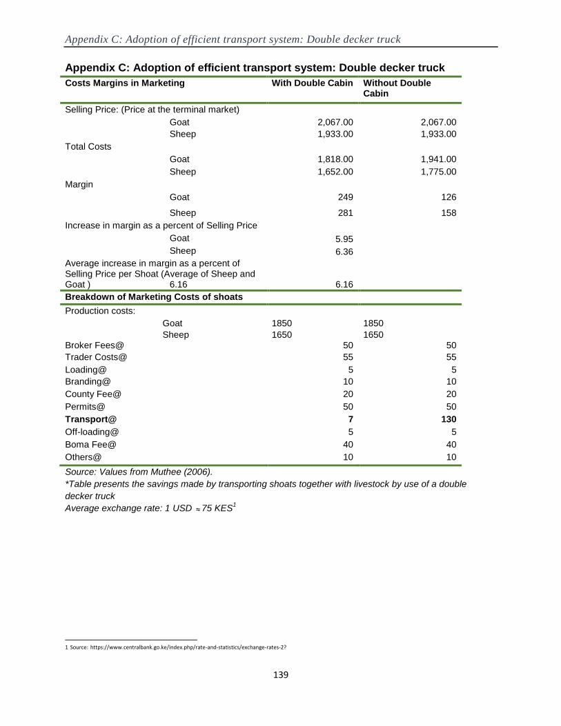
Appendix C: Adoption of efficient transport system: Double decker truck
139
Appendix C: Adoption of efficient transport system: Double decker truck
Costs Margins in Marketing With Double Cabin Without Double Cabin
Selling Price: (Price at the terminal market)
Goat 2,067.00 2,067.00
Sheep 1,933.00 1,933.00
Total Costs
Goat 1,818.00 1,941.00
Sheep 1,652.00 1,775.00
Margin
Goat 249 126
Sheep 281 158
Increase in margin as a percent of Selling Price
Goat 5.95
Sheep 6.36
Average increase in margin as a percent of Selling Price per Shoat (Average of Sheep and Goat ) 6.16 6.16
Breakdown of Marketing Costs of shoats
Production costs:
Goat 1850 1850
Sheep 1650 1650 Broker Fees@ 50 50
Trader Costs@ 55 55
Loading@ 5 5
Branding@ 10 10
County Fee@ 20 20
Permits@ 50 50
Transport@ 7 130
Off-loading@ 5 5
Boma Fee@ 40 40
Others@ 10 10
Source: Values from Muthee (2006).
*Table presents the savings made by transporting shoats together with livestock by use of a double
decker truck
Average exchange rate: 1 USD 75 KES1
1 Source:
https://www.centralbank.go.ke/index.php/rate-and-statistics/exchange-rates-2?

Appendix D: Detailed lists of sets, parameters, scalars, variables, and equations in the
model.
140
Appendix D: Detailed lists of sets, parameters, scalars, variables, and
equations in the model.
PMP MODEL
SETS
I PRODUCTION PROCESSES
II(I) INTENSIVE PRODUCTION
J RESOURCE SUB SET
R(J) LAND INPUT
P(J) CROP RESOURCE SUB SET
ITEMS ITEMS INCORPORATED IN THE SIMULATION
ALIAS (J,L)
PARAMETERS
PRI(I) CROP PRICES (KSH PER KG)
Y(I) CROP YIELD (KG PER HECTARE)
TABLE C(I,J) COST (KSH PER UNIT) OF FIXED PRODUCTION FACTORS
TABLE A(I,J) A MATRIX OF TECHNICAL COEFFICIENTS/ QUANTITY OF INPUTS (J)
THAT TRANSLATE INTO PHYSICAL OUTPUT PER HECTARE
XBASE(I) BASE/INITIAL LAND ALLOCATIONS
B(J) RESOURCE CONSTRAINTS
XB(I,J) TOTAL BASE QUANTITY OF RESOURCES USED
XB(I,J) = A(I,J) * XBASE(I) ;
REV(I) REVENUE
REV(I) = PRI(I)* Y(I) ;
CSL(I) LINEAR COST:
CSL(I) = SUM(J, C(I,J)*A(I,J));
NET(I) NET RETURN:
NET(I) = REV(I)- CSL(I);
PERDIFF1(I) DIFFERENCE BETWEEN LINEAR PROGRAM LAND USE AND
BASELINE OBSERVATIONS
PERDIFF1(I)$XB(I,"LAND") = ((LX.L(I)- XB(I,"LAND"))*100)/ XB(I,"LAND")
;
SUB ELASTICITY OF SUBSTITUTION
ADJ ADJUSTMENT FOR MARGINAL CROPS
ADJ = RESOURCE.M("LAND") * ADJFACT;
OPP(J) OPPORTUNITY COST OF LAND
OPP(J)= RESOURCE.M(J) ;
OPP("LAND")= RESOURCE.M("LAND") - ADJ;
LAM(I,J) PMP DUAL VALUE ON LAND
LAM(I,"LAND") = CALIB.M(I) + ADJ ;
TOT(I) TOTAL OUTPUT
TOT(I) = Y(I)*XB(I,"LAND") ;
CST(I,J) COST OF FIXED PRODUCTION FACTORS PLUS OPPORTUNITYCOST

Appendix D: Detailed lists of sets, parameters, scalars, variables, and equations in the
model.
141
CST(I,J) = C(I,J) + OPP(J) + LAM(I,J) ;
ETA(I) FUNCTION OF ELASTICITY OF SUBSTITUTION
ETA(I) = (SUB - 1)/SUB ;
THETA MINUS ONE OVER ELASTICITY OF SUBSTITUTION
THETA = -(1/SUB) ;
BETA(I,J) SHARE PARAMETERS
BETA(II,J)$(SW(J) EQ 1) = 1/( SUM(P, (CST(II,P)/CST(II,J)) *
( XB(II,J)/XB(II,P))**THETA ) + 1 ) ;
BETA(II,J)$(SW(J) EQ 2) = 1 - SUM(L$(SW(L) NE 2), BETA(II,L) ) ;
BETA(II,J)$(SW(J) EQ 0) = SUM(R,BETA(II,R))*(CST(II,J)/
SUM(R,CST(II,R)))* (SUM(R, XB(II,R))/XB(II,J))**THETA ;
CN(I) SCALE PARAMETER
CN(II) = TOT(II) / (SUM(J, BETA(II,J)*
((XB(II,J)+0.0001)**((SUB-1)/SUB )))** (SUB/(SUB-1))) ;
NI(J) RESOURCE COUNTER
NI(J) = ORD(J);
MARPRO2(I,J) MARGINAL PRODUCT
MARPRO2(II,J) = BETA(II,J)*(CN(II)**ETA(II))* (TOT(II)/XB(II,J))**(1/SUB)
;
VMP2(I,J) VALUE MARGINAL PRODUCT
VMP2(II,J) = MARPRO2(II,J)* PRI(II) ;
ALPH(I) COST INTERCEPT
ALPH(I) = C(I,"LAND") - LAM(I,"LAND")
GAM(I) COST SLOPE
GAM(I)$(LAM(I,"LAND") NE 0 ) = (2* LAM(I,"LAND"))
/XBASE(I)
PMPTEST(I) TEST VALUE FROM PMP
PMPTEST(I) = ALPH(I)+ GAM(I)*XBASE(I) ;
PMPDIFF(I) PERCENT DEVIATION IN PMP
PMPDIFF(I)$LAM(I,"LAND") = (( PMPTEST(I)- LAM(I,"LAND"))*100)/
LAM(I,"LAND")
VMPDIFF(II,J) VALUE MARGINAL PRODUCT CHECK
VMPDIFF(II,J)$CST(II,J) = (( VMP2(II,J)- CST(II,J))*100)/ CST(II,J);
PERDIF2(I,J) PERCENT DIFFERENCE BETWEEN CALIBRATED NON-LINEAR
MODEL INPUT ALLOCATION AND OBSERVED BASE INPUT
ALLOCATION
PERDIF2(I,J)$XB(I,J) = (XC.L(I,J) - XB(I,J)) * 100 / XB(I,J) ;
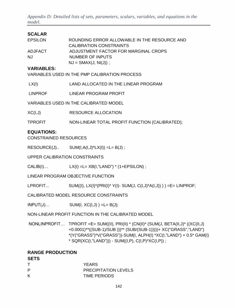
Appendix D: Detailed lists of sets, parameters, scalars, variables, and equations in the
model.
142
SCALAR
EPSILON ROUNDING ERROR ALLOWABLE IN THE RESOURCE AND
CALIBRATION CONSTRAINTS
ADJFACT ADJUSTMENT FACTOR FOR MARGINAL CROPS
NJ NUMBER OF INPUTS
NJ = SMAX(J, NI(J)) ;
VARIABLES:
VARIABLES USED IN THE PMP CALIBRATION PROCESS
LX(I) LAND ALLOCATED IN THE LINEAR PROGRAM
LINPROF LINEAR PROGRAM PROFIT
VARIABLES USED IN THE CALIBRATED MODEL
XC(I,J) RESOURCE ALLOCATION
TPROFIT NON-LINEAR TOTAL PROFIT FUNCTION (CALIBRATED);
EQUATIONS:
CONSTRAINED RESOURCES
RESOURCE(J).. SUM(I,A(I,J)*LX(I)) =L= B(J) ;
UPPER CALIBRATION CONSTRAINTS
CALIB(I)… LX(I) =L= XB(I,"LAND") * (1+EPSILON) ;
LINEAR PROGRAM OBJECTIVE FUNCTION
LPROFIT... SUM((I), LX(I)*(PRI(I)* Y(I)- SUM(J, C(I,J)*A(I,J)) ) ) =E= LINPROF;
CALIBRATED MODEL RESOURCE CONSTRAINTS
INPUT(J)… SUM(I, XC(I,J) ) =L= B(J);
NON-LINEAR PROFIT FUNCTION IN THE CALIBRATED MODEL
NONLINPROFIT… TPROFIT =E= SUM((II), PRI(II) * (CN(II)* (SUM(J, BETA(II,J)* ((XC(II,J)
+0.0001)**((SUB-1)/SUB )))** (SUB/(SUB-1)))))+ XC("GRASS","LAND")
*(Y("GRASS")*V("GRASS"))-SUM(I, ALPH(I) *XC(I,"LAND") + 0.5* GAM(I)
* SQR(XC(I,"LAND"))) - SUM((I,P), C(I,P)*XC(I,P)) ;
RANGE PRODUCTION
SETS
T YEARS
P PRECIPITATION LEVELS
K TIME PERIODS

Appendix D: Detailed lists of sets, parameters, scalars, variables, and equations in the
model.
143
W RAINY SEASONS
BASET(K) FIRST PERIOD
ROOT(N) THE ROOT NODE
KW(K,W) RELATING TIME PERIODS TO RAINY SEASONS
N NODES: DECISION POINTS OR STATES IN SCENARIO TREE
KN(K,N) MAP NODES TO TIME PERIODS
ANC(CHILD,PARENT) ANCESTOR MAPPING
NP(N,P) MAPS NODES TO PRECIPITATION LEVEL
LEAF(N)
ITER MAX NUMBER OF ITERATIONS
I NODES AT WHICH VALUE FUNCTION IS EVALUATED
ALIAS (N,PARENT,CHILD)
ALIAS (I,J)
TABLE
RAINFALL(W,P) RAINFALL AMOUNT FOR EACH SEASON
PARAMETERS
PR(P) PROBABILITY DISTRIBUTION OVER RAINFALL LEVELS
NPROB(N) PROBABILITY OF BEING AT ANY NODE
NDELTA(N) RAINFALL AT EACH NODE
R(T) RAINFALL SCENARIOS (AMOUNTS AT THE NODE OF
SCENARIO TREE FORM THE RAINFALL SCENARIOS)
DEF DEFAULT VALUE
BETA(T) DISCOUNT FACTOR
BETA(T) = 1/(1+ IR)**ORD(T);
BETA(T) = BETA("1");
TLU0 TROPICAL LIVESTOCK UNITS IN PREVIOUS PERIOD
TLU0 = STOCK(I) ;
BETA0 CURRENT BETA
BETA0 = BETA("1");
RAIN RAIN IN CURRENT PERIOD
X(I) NODE VALUE FOR THE STATE VARIABLE ON THE UNIT
INTERVAL
X(J) = COS(ARG(J)) ;
IN(I) INDICES TO CALCULATE THE ARGUMENT OF THE COSINE
WEIGHTING FUNCTION
IN(I) = ORD(I);
IMAX = SMAX(I, IN(I)) ;
AOLD(J) PREVIOUS POLYNOMIAL COEFFICIENT VALUE FOR LOOP
CONVERGENCE CHECK
AOLD(I) = ACOEF(I);
STOCK(J) STOCK LEVEL VALUE AT NODE J FOR GRID POINT
CALCULATION

Appendix D: Detailed lists of sets, parameters, scalars, variables, and equations in the
model.
144
STOCK(J) = (L+U+(U-L)*X(J))/2;
VAL(J) STORES THE VALUE OF THE VALUE FUNCTION FOR LOOP
CALCULATION
PHIBAR(I,J) POLYNOMIAL TERMS USED IN THE LOOP CONVERGENCE
CALCULATION
PHIBAR("1",J) = 1;
PHIBAR("2",J) = X(J);
LOOP(I$(ORD(I) GE 3), PHIBAR(I,J) = 2*X(J)*PHIBAR(I-1,J)-
PHIBAR(I- 2,J) ) ;
ARG(J) ARGUMENT OF THE COSINE WEIGHTING FUNCTION
ARG(J) = ((2*IN(J)-1)*PI)/(2*IMAX)
ACOEF(I) INITIAL POLYNOMIAL COEFFICIENT VALUES FOR VALUE
FUNCTION
ACOEF(I) = 0;
ACOEF(I)$SUM(J,SQR(PHIBAR(I,J))) = SUM(J,
VAL(J)*PHIBAR(I,J)) / SUM(J,SQR(PHIBAR(I,J))) ;
DIFF(ITER) DEVIATION OF CHEBYCHEV COEFFICIENTS FOR EACH
VALUE ITERATION
DIFF(ITER)= TEST;
CPOLY(ITER,I) CHEBYCHEV POLYNOMIAL COEFFICIENTS AT EACH
ITERATION
CPOLY(ITER,I)= ACOEF(I);
CVALUES(ITER,I,*) COEFFICIENT VALUES FOR CHEBYCHEV POLYNOMIALS
CVALUES(ITER,I,'CERROR') = DIFF(ITER) ;
CVALUES(ITER,I,'CCOEF_VALUEFCN') = CPOLY(ITER,I);
SCALAR
LAM GROWTH RATE OF LIVESTOCK HERD
AREA RANGE AREA IN HA
PH FEEDING REQUIREMENTS OF A TLU KG DM/TLU PER YEAR
VC VARIABLE COST PER TLU (INPUT COSTS TO MAINTAIN THE
HERD)
IR THE DISCOUNT RATE
BOSH 'PROPER-USE FACTOR' FORAGE ALLOWANCE
BINS ADJUSTMENT FACTOR FOR BIOMASS SHARE USED BY
OTHER LIVESTOCK AND NON-LIVESTOCK USES
TEST TEST FOR CONVERGENCE
TEST = SUM(I,(ACOEF(I)-AOLD(I))*(ACOEF(I)-AOLD(I)));
TOL TOLERANCE FOR CONVERGENCE
IMAX LARGEST INTEGER IN SET I
PI ...14.3 ;
U UPPER LIMIT ON CARRY-OVER STOCK
L LOWER LIMIT ON CARRY-OVER STOCK

Appendix D: Detailed lists of sets, parameters, scalars, variables, and equations in the
model.
145
VARIABLES
CVB CURRENT VALUE BENEFIT
PHI(J) NODAL APPROXIMATIONS OF VALUE FUNCTION
VALUEFCN VALUE FUNCTION
SL OPTIMAL SALES
ANPP ABOVEGROUND NET PRIMARY PRODUCTIVITY (ANPP, KG DM/HA
SRATE STOCKING DENSITY
TLU TROPICAL LIVSTCK UNITS IN NEXT PERIOD
MTLU MAXIMUM GRAZING CAPACITY
FOD FODDER
PROFIT TOTAL CURRENT PROFITS
EQUATIONS
ABOVEGROUND NET PRIMARY PRODUCTIVITY (ANPP, KG DM/HA)
RUEEQN.. ANPP =E=-1000 + 7.5*RAIN-SRATE*(-1000+7.5*RAIN) ;
STOCKING DENSITY
STOCKEQN.. SRATE =E= TLU/ AREA
LIVESTOCK DYNAMICS
TLUEQN.. TLU=E= TLU0+( LAM *( 1-( TLU0/MTLU))*TLU0 )- SL;
MAXIMUM GRAZING CAPACITY
MAXEQN.. MTLU =E= FOD/PH ;
FODDER PRODUCTION
FODEQN.. FOD =E= (ANPP* AREA*BOSH)*BINS ;
CURRENTPROFITS
PROFITEQN.. PROFIT =E= SL*(INTERCEPT- SLOPE *SL )-SALES *VC;
POLYNOMIAL RECURSION EQUATION 1
PHI1.. PHI("1") =E= 1 ;
POLYNOMIAL RECURSION EQUATION 2
PHI2.. PHI("2") =E= ((TLU-(L+U)/2)/((U-L)/2)) ;
POLYNOMIAL RECURSION EQUATION 3
PHI3(J)$(ORD(J) GE 3).. PHI(J) =E= 2*((TLU-(L+U)/2)/((U-L)/2))*PHI(J-1)-PHI(J-2) ;
VALUE FUNCTION FOR SIMULATION STAGE
VFN.. VALUEFCN =E= SUM(J, ACOEF(J) * PHI(J)) ;
PRESENT VALUE BENEFIT FUNCTION WITH CHEBYCHEV APPROXIMATION
CVBFCN .. CVB =E= PROFIT + BETAO*VALUEFCN.

Appendix E: Principal Component Analysis Results
146
Appendix E: Principal Component Analysis
Table E.1: Principal component analysis on degree of capabilities
Variable description Mean Std.Dev. Factor Scores/ Weights for Each Variable
Years of Schooling 5.600 4.845 0.4028 Literate 0.481 0.500 0.3613 Level of education attained 0.713 0.878 0.4008
Main walling material 0.153 0.361 0.2083 Main roofing material 0.572 0.495 0.2951 Toilet facility 0.298 0.458 0.2878 Lighting 0.100 0.301 0.1762 No. of people living in one house (measure of living in crowded conditions) 6.233 3.024 -0.0092
Access to the health center 4.786 4.160 -0.2649 Access to drinking water 2.332 1.592 -0.2815 Source of drinking water(protected and covered)
0.489 0.500 0.2829
Sufficiency of household food consumption
2.916 0.817 0.2696
kmo 0.864 Largest Eigenvalue,λ 5.158 Proportion of Variance Explained 0.430
Table E.2: Principal component analysis on relative wealth index (material wealth
index)
Variable description Mean Std.Dev. Factor Scores/ Weights for Each Variable
Plough 0.067 0.250 0.201 Donkey/ox cart 0.019 0.138 0.150 Wheel barrow 0.180 0.385 0.319 Tractor 0.012 0.109 0.219 Cattleshed 0.387 0.488 0.352
Bicycle 0.043 0.204 0.184 Radio 0.385 0.487 0.390 Television 0.070 0.255 0.310 Car 0.031 0.174 0.282 Mobile phone 0.447 0.498 0.406 Water tank 0.091 0.288 0.315 Motorcycle 0.053 0.224 0.199
Kmo 0.764 Largest Eigenvalue,λ 3.717 Proportion of Variance Explained 0.310
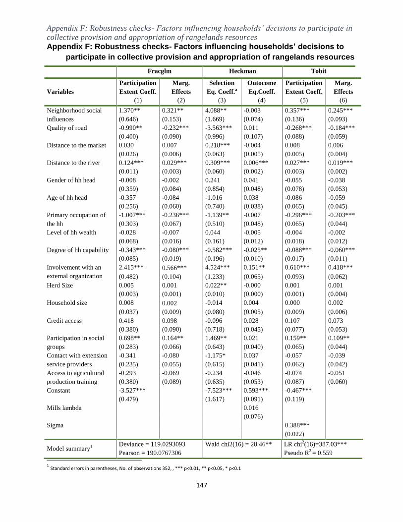
Appendix F: Robustness checks- Factors influencing households’ decisions to participate in
collective provision and appropriation of rangelands resources
147
Appendix F: Robustness checks- Factors influencing households’ decisions to
participate in collective provision and appropriation of rangelands resources
1 Standard errors in parentheses, No. of observations 352, , *** p<0.01, ** p<0.05, * p<0.1
Fracglm Heckman Tobit
Variables
Participation
Extent Coeff.
(1)
Marg.
Effects
(2)
Selection
Eq. Coeff.a
(3)
Outocome
Eq.Coeff.
(4)
Participation
Extent Coeff.
(5)
Marg.
Effects
(6)
Neighborhood social
influences
1.370** 0.321** 4.088** -0.003 0.357*** 0.245***
(0.646) (0.153) (1.669) (0.074) (0.136) (0.093)
Quality of road -0.990** -0.232*** -3.563*** 0.011 -0.268*** -0.184***
(0.400) (0.090) (0.996) (0.107) (0.088) (0.059)
Distance to the market 0.030 0.007 0.218*** -0.004 0.008 0.006
(0.026) (0.006) (0.063) (0.005) (0.005) (0.004)
Distance to the river 0.124*** 0.029*** 0.309*** 0.006*** 0.027*** 0.019***
(0.011) (0.003) (0.060) (0.002) (0.003) (0.002)
Gender of hh head -0.008 -0.002 0.241 0.041 -0.055 -0.038
(0.359) (0.084) (0.854) (0.048) (0.078) (0.053)
Age of hh head -0.357 -0.084 -1.016 0.038 -0.086 -0.059
(0.256) (0.060) (0.740) (0.038) (0.065) (0.045)
Primary occupation of
the hh
-1.007*** -0.236*** -1.139** -0.007 -0.296*** -0.203***
(0.303) (0.067) (0.510) (0.048) (0.065) (0.044)
Level of hh wealth -0.028 -0.007 0.044 -0.005 -0.004 -0.002
(0.068) (0.016) (0.161) (0.012) (0.018) (0.012)
Degree of hh capability -0.343*** -0.080*** -0.582*** -0.025** -0.088*** -0.060***
(0.085) (0.019) (0.196) (0.010) (0.017) (0.011)
Involvement with an
external organization
2.415*** 0.566*** 4.524*** 0.151** 0.610*** 0.418***
(0.482) (0.104) (1.233) (0.065) (0.093) (0.062)
Herd Size 0.005 0.001 0.022** -0.000 0.001 0.001
(0.003) (0.001) (0.010) (0.000) (0.001) (0.004)
Household size 0.008 0.002 -0.014 0.004 0.000 0.002
(0.037) (0.009) (0.080) (0.005) (0.009) (0.006)
Credit access 0.418 0.098 -0.096 0.028 0.107 0.073
(0.380) (0.090) (0.718) (0.045) (0.077) (0.053)
Participation in social
groups
0.698** 0.164** 1.469** 0.021 0.159** 0.109**
(0.283) (0.066) (0.643) (0.040) (0.065) (0.044)
Contact with extension
service providers
-0.341 -0.080 -1.175* 0.037 -0.057 -0.039
(0.235) (0.055) (0.615) (0.041) (0.062) (0.042)
Access to agricultural
production training
-0.293 -0.069 -0.234 -0.046 -0.074 -0.051
(0.380) (0.089) (0.635) (0.053) (0.087) (0.060)
Constant -3.527*** -7.523*** 0.593*** -0.467***
(0.479) (1.617) (0.091) (0.119)
Mills lambda 0.016
(0.076)
Sigma 0.388***
(0.022)
Model summary1
Deviance = 119.0293093
Pearson = 190.0767306
Wald chi2(16) = 28.46** LR chi2(16)=387.03***
Pseudo R2 = 0.559

Appendix G: Survey Instrument
148
Appendix G: Survey Instrument
Pastoralists and Agro pastoralists in Narok County Survey, 2013/2014
Collective Action Initiatives Interview Schedule
INTERVIEW WITH INDIVIDUAL PASTORAL AND AGRO-PASTORAL
HOUSEHOLDS
Good morning/afternoon. My name is _________________. I am conducting a survey
for ZEF Germany, in collaboration with KARI as part of a larger research initiative on
Economics of Land Degradation. The study aims at evaluating the effect of collective
action initiatives/groups in the region have on livelihoods and sustainable
management of rangelands. I would like to request your participation in this short
interview. Any information you provide will be strictly confidential and will not be used
for any purpose outside of this research.
STARTING TIME…………………………………………
PART 0. INTERVIEW BACKGROUND
1. Date of interview: Day: …..……………… Month: ........................ Year: …………….….…..….…
2. Interviewed by (enumerator‘s name): ………...............................................................................
3. Supervised by............................................4. County...................................................................
5. Division …………………………….. 6. Location………………………………………………………
7. Sub-Location………………………………………..8. Village.........................................................
9. GPS readings of village: a) Altitude..................; b) Latitude……………; c) Longitude……..……

Appendix G: Survey Instrument
149
PART 1: RESPONDENT IDENTIFICATION AND VILLAGE CHARACTERISTICS
1. Name of respondent........................................................................................................................
2. Marital Status (Codes A) .....................Sex (Codes B).....................Age (years)............................
3. Relation to household head..............................................................................................................
4. Highest Education Level (Codes C).................................................................................................
5. Major family language………...........................................................................................................
6. Religion of the household head (Codes D)......................................................................................
7. Primary occupation of the household (Codes E)………...…………...……………………………..
8. Secondary occupation of Household (Codes E)…….………………………………………………
9. Taking into consideration ALL your food sources (own food production + food purchase + help
from different sources + food hunted from forest etc.), how would you define your family‘s
food consumption last year? (Codes F)....................................................................................
10. Distance to the nearest neighbour (Km)…………......minutes of walking time……………………
11. Distance to the nearest main market from residence (km)……minutes of walking time………...…
12. Quality of road to the main market (Codes G)……….………..........................................................
13. Average single transport cost (per person) to the main market using a car (KSh/person)..............
14. Distance to the nearest agricultural extension office from residence (km)……..minutes of walking
time.
15. Distance to the nearest health center from residence (km)… ……minutes of walking time….........
16. Distance to the nearest primary school (km)……………………minutes of walking time…...........
17. Distance to the nearest secondary school (km)…………………minutes of walking time…............
18. Main source of drinking water………...............................................................................(Codes H)
19. Main source of livestock water…………………..............................................................(Codes H)
20. Distance to main water source for drinking from residence (km)….…minutes of walking time…..
21. Distance to nearest river from residence (km)……….….…minutes of walking time…….………..
Codes A: 1.Single, 2.married, 3.widowed, 4.separated, 5.divorced
Codes B: 1. Female; 2. Male
Codes C: 1. None; 2.Primary; 3. Secondary; 4. College/Institute; 5. University; 6. Other, specify……………………………
Codes D: 1. No religion/atheist; 2. Orthodox Christian; 3. Catholic; 4. Protestant; 5. Other Christian 6. Muslim; 7. Other, specify………...……
Codes E: 1.Herding, 2.livestock framing 3.crop farming 4.poultry farming, 5.salaried employment, 6.self-employed off-farm, 7. casual laborer on-farm, 8.casual laborer off-farm,
9.household chores, 10.apiculture, 11.aquaculture, 12.other, specify..............
Codes F: 1. Food shortage throughout the year, 2. Occasional food shortage, 3. No food shortage but no surplus, 4. Food surplus.
Codes G: 1= Very poor; 2= Poor; 3= Average; 4=Good; 5= Very good;
Codes H: 1. Piped; 2. Borehole protected and covered; 3. Borehole unprotected & uncovered; 4. Stream; 5. River; 6. Lake; 7. Ponds/dams or floods/Water Pans; 8. Harvested rain
water; 9. Others (Specify)……… Note: protected refers to water sources internally plastered and covered with a cap of wood, stone or concrete).
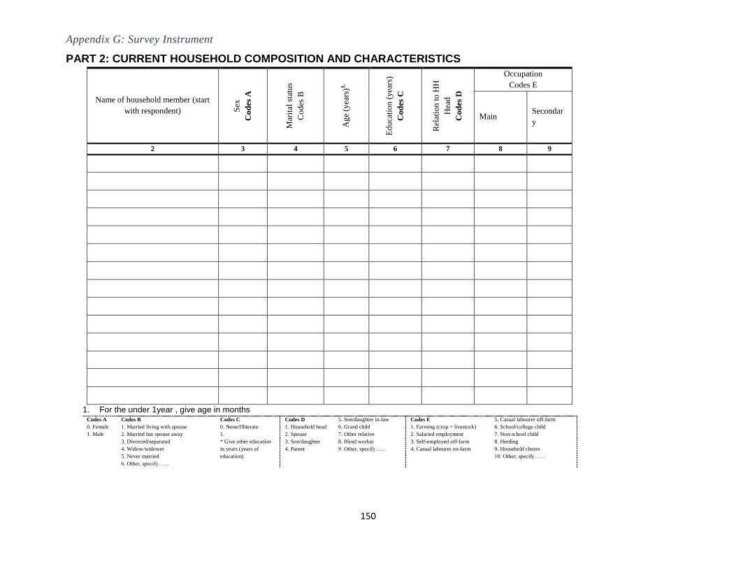
Appendix G: Survey Instrument
150
PART 2: CURRENT HOUSEHOLD COMPOSITION AND CHARACTERISTICS
Name of household member (start
with respondent) Sex
Co
des
A
Mar
ital
sta
tus
Co
des
B
Ag
e (y
ears
)1.
Ed
uca
tion
(y
ears
)
Co
des
C
Rel
atio
n t
o H
H
Hea
d
Co
des
D
Occupation
Codes E
Main Secondar
y
2 3 4 5 6 7 8 9
1. For the under 1year , give age in months Codes A
0. Female
1. Male
Codes B
1. Married living with spouse
2. Married but spouse away
3. Divorced/separated
4. Widow/widower
5. Never married
6. Other, specify……
Codes C
0. None/Illiterate
1.
* Give other education
in years (years of
education)
Codes D
1. Household head
2. Spouse
3. Son/daughter
4. Parent
5. Son/daughter in-law
6. Grand child
7. Other relative
8. Hired worker
9. Other, specify……
Codes E
1. Farming (crop + livestock)
2. Salaried employment
3. Self-employed off-farm
4. Casual labourer on-farm
5. Casual labourer off-farm
6. School/college child
7. Non-school child
8. Herding
9. Household chores
10. Other, specify……

Appendix G: Survey Instrument
151
PART 3: SOCIAL CAPITAL, TRUST, NETWORKING AND COLLECTIVE ACTION INITIATIVES: TO BE FILLED FOR
HOUSEHOLDS WITH AN ADULT HOUSEHOLD MEMBER IN A COLLECTIV ACTION INITIATIVE/GROUP
SECTION A: MEMBERSHIP IN A COLLECTIVE ACTION INITIATIVE
1. Which adults in your household (including you) are members of a collective action group? (One group membership per row.)
Name of
family
member
Relation to
HH head
Type of group
the hh member
is/was a
member of:
(codes A)
Three most important
group functions: (codes
B)
Year
joined
(YYYY)
Role in
the group
(codes C)
Still a
member
now?
(codes D)
If No in column 8, reason/s for
leaving the group (codes E),
Rank 3
1st 2nd 3rd 1st 2nd 3rd
1 2 3 4 5 6 7 8 9 10 11
Codes A
1. Conservancy
2.Water User’s Association
3. Livestock producer and marketing
group/coops
4. Farmers’ Association
5. Women’s Association
6. Youth Association
7. Saving and credit group
8. Microenterprise development (i.e., milk
processing, poultry production, apiculture,
handicraft initiatives, etc.)
9. Farmer research group
10. Other, specify……
Codes B
1.Microfinance/ Savings and credit
2. Produce marketing (crop and livestock)
3. Briquette making
4.Tree planting and establishing community nurseries
5. poultry production,
6. apiculture
7.aquaculture
8.handicraft initiatives
9. River bank protection and rehabilitation of eroded sites
10. Tourism Investment /wildlife tourism and recreation
11.Input access/marketing
12. Seed production
13. Develop and finance maintenance of boreholes,
earthen dams and water pans
14. Maintaining public spaces, e.g. roads
15Investment in human health,
16. Investment in formal education
17.Grain milling
18.Butcheries,
19 Tanneries
20.Bakeries,
21. Other, specify………
Codes C
1. Official
2. Ex-
official
3. Ordinary
member
Codes D
1. Yes
0. No
Codes E
1. Left because
organization was not
useful/profitable
2. Left because of poor
management
3. Unable to pay annual
subscription fee
4. Group ceased to exist
5. Other,
specify……………
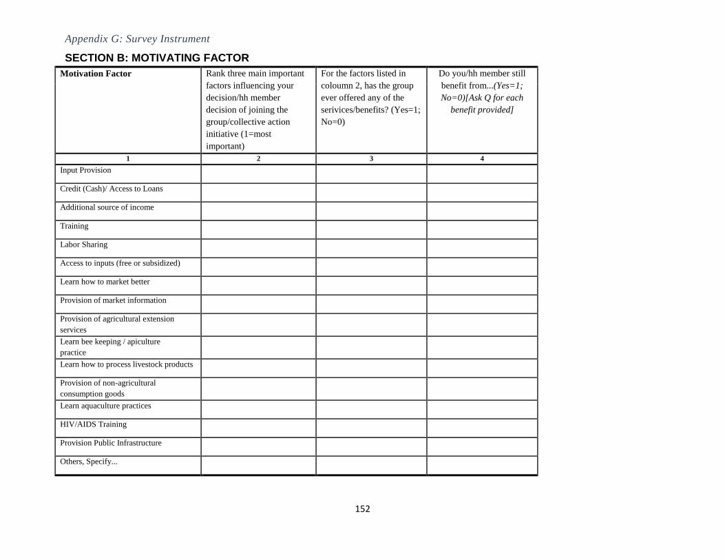
Appendix G: Survey Instrument
152
SECTION B: MOTIVATING FACTOR
Motivation Factor
Rank three main important
factors influencing your
decision/hh member
decision of joining the
group/collective action
initiative (1=most
important)
For the factors listed in
coloumn 2, has the group
ever offered any of the
serivices/benefits? (Yes=1;
No=0)
Do you/hh member still
benefit from...(Yes=1;
No=0)[Ask Q for each
benefit provided]
1 2 3 4
Input Provision
Credit (Cash)/ Access to Loans
Additional source of income
Training
Labor Sharing
Access to inputs (free or subsidized)
Learn how to market better
Provision of market information
Provision of agricultural extension
services
Learn bee keeping / apiculture
practice
Learn how to process livestock products
Provision of non-agricultural
consumption goods
Learn aquaculture practices
HIV/AIDS Training
Provision Public Infrastructure
Others, Specify...

Appendix G: Survey Instrument
153
SECTION C: ECONOMIC CONTROL, TRAINING, SOCIAL CAPITAL AND NETWORKING
1. Do the group(s)/collective action initiative(s) that you and /or the other members of your hh belong to provide
any training for its members?
(Yes=1, No=0)
2. If the group is providing training, who sponsors the training? (Government; Non-Governmental Organizations; Group own
funds; Others (Specify)…… ……….
3. If the group is providing training, what type of training is it? Please list ………………………………………..
4. Can non-members access this training? (Yes=1, No=0)
5. If non-members access training, what is the main/most important condition for accessing training for non-
members? Please state
6. Has your household gained any financial benefits from the group(s) that you or any other adult member of
your household belongs to? (If Yes continue; if No skip to 7)
(Yes=1, No=0)
7. Approximately how much financial benefit in money did your household receive in the last 12 months? (Kshs)………...
8. Does the collective action initiative/group provide cash advances? (Yes=1, No=0)
9. If yes, how frequently have you received cash advance? (Monthly, Every six months, Other
(Specify)...............................
10. Are there any criteria for getting cash advance from the group? (Yes=1, No=0)
11. What is the most important criteria? Please state …………………………..
12. What happens to defaulters? Please state ………………………………….
13. Who within your household makes decisions about what to do with the financial benefits gained from the
group(s)?
(1 = Wife 2 = My husband 3 = Wife and my husband, jointly)
14. Have you spent the financial benefits from the group(s) you and/or your hh members gained from the
group(s)? [If YES continue to 14, if No move to 16]
(Yes=1; No=0)
15. How much was spent? (Kshs)………...
16. On what were the financial benefits spent on? ..........., ............, .............
17. Have you noticed any change in your household’s wellbeing since you and/or your hh members joined the
group(s)?
(Yes=1; No=0)
18. Have you noticed any change in the ability of your hh to access credit/capital since you and/or your hh
members joined the group(s)?
(Yes=1; No=0)
19. Could you explain how your ability to access credit/capital has changed since you and/or your hh members
joined the group(s)?
.................................................
20. Have you noticed a change in your ability to create useful networks of people in your community since you
and/or your hh members joined the group(s)?
(Yes=1; No=0)
21. Could you explain how your social networks in the community changed since you and/or your hh members
joined the group(s)?
.................................................................
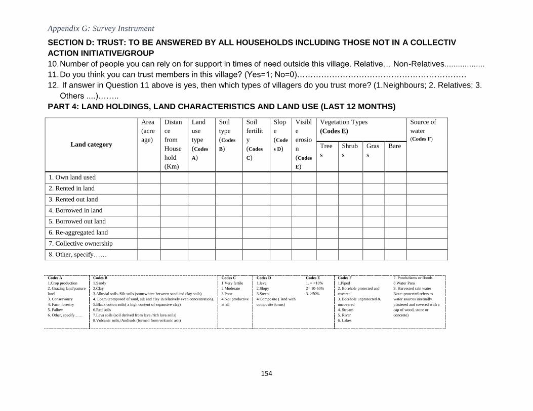
Appendix G: Survey Instrument
154
SECTION D: TRUST: TO BE ANSWERED BY ALL HOUSEHOLDS INCLUDING THOSE NOT IN A COLLECTIV
ACTION INITIATIVE/GROUP
10. Number of people you can rely on for support in times of need outside this village. Relative… Non-Relatives..................
11. Do you think you can trust members in this village? (Yes=1; No=0)………………………………………………………
12. If answer in Question 11 above is yes, then which types of villagers do you trust more? (1.Neighbours; 2. Relatives; 3.
Others ....)……..
PART 4: LAND HOLDINGS, LAND CHARACTERISTICS AND LAND USE (LAST 12 MONTHS)
Land category
Area
(acre
age)
Distan
ce
from
House
hold
(Km)
Land
use
type
(Codes
A)
Soil
type
(Codes
B)
Soil
fertilit
y
(Codes
C)
Slop
e
(Code
s D)
Visibl
e
erosio
n
(Codes
E)
Vegetation Types
(Codes E)
Source of
water
(Codes F) Tree
s
Shrub
s
Gras
s
Bare
1. Own land used
2. Rented in land
3. Rented out land
4. Borrowed in land
5. Borrowed out land
6. Re-aggregated land
7. Collective ownership
8. Other, specify……
Codes A
1.Crop production
2. Grazing land/pasture
land
3. Conservancy
4. Farm forestry
5. Fallow
6. Other, specify……
Codes B
1.Sandy
2.Clay
3.Alluvial soils /Silt soils (somewhere between sand and clay soils)
4. Loam (composed of sand, silt and clay in relatively even concentration).
5.Black cotton soils( a high content of expansive clay)
6.Red soils
7.Lava soils (soil derived from lava /rich lava soils)
8.Volcanic soils,/Andisols (formed from volcanic ash)
Codes C
1.Very fertile
2.Moderate
3.Poor
4.Not productive
at all
Codes D
1.level
2.Slopy
3.Steep
4.Composite ( land with
composite forms)
Codes E
1. = <10%
2= 10-50%
3. >50%
Codes F
1.Piped
2. Borehole protected and
covered
3. Borehole unprotected &
uncovered
4. Stream
5. River
6. Lakes
7. Ponds/dams or floods.
8.Water Pans
9. Harvested rain water
Note: protected refers to
water sources internally
plastered and covered with a
cap of wood, stone or
concrete)
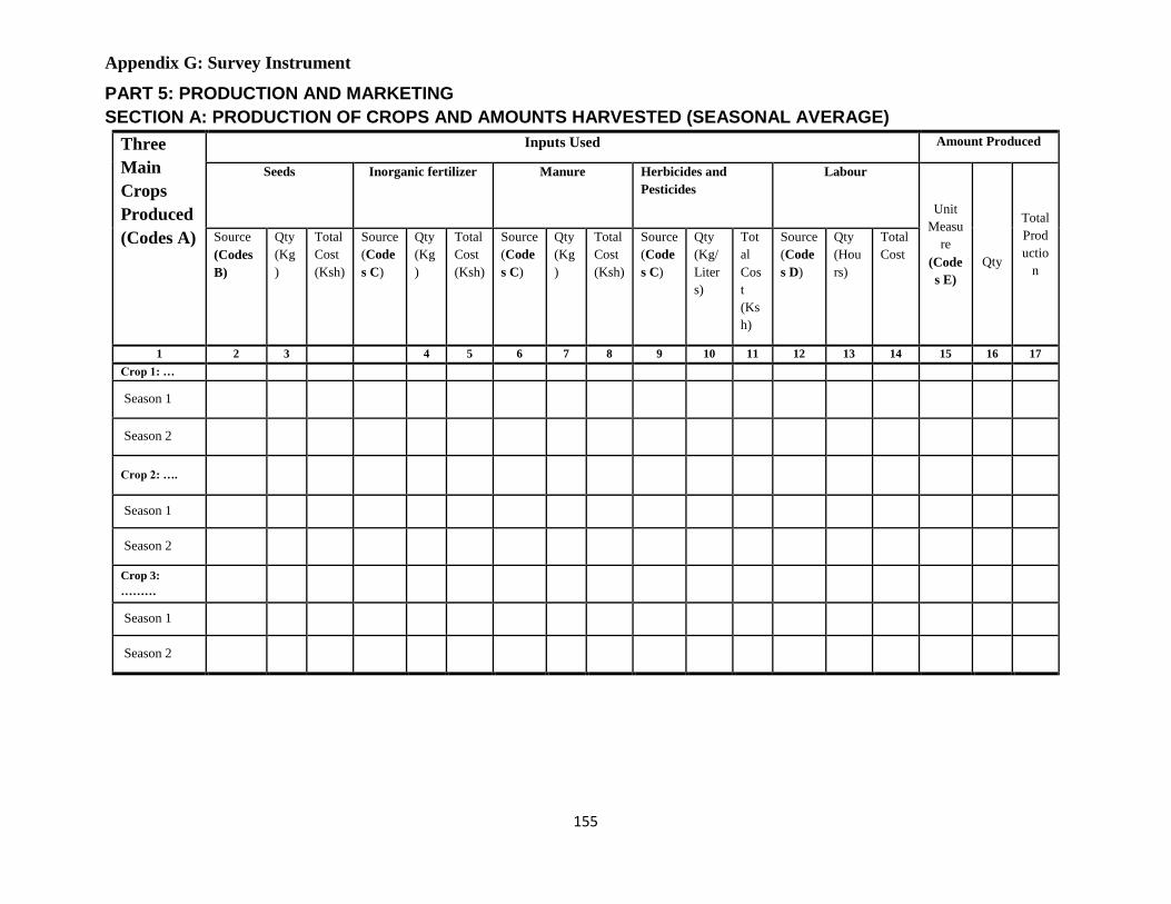
Appendix G: Survey Instrument
155
PART 5: PRODUCTION AND MARKETING
SECTION A: PRODUCTION OF CROPS AND AMOUNTS HARVESTED (SEASONAL AVERAGE)
Three
Main
Crops
Produced
(Codes A)
Inputs Used Amount Produced
Seeds Inorganic fertilizer Manure Herbicides and
Pesticides
Labour
Unit
Measu
re
(Code
s E)
Qty
Total
Prod
uctio
n
Source
(Codes
B)
Qty
(Kg
)
Total
Cost
(Ksh)
Source
(Code
s C)
Qty
(Kg
)
Total
Cost
(Ksh)
Source
(Code
s C)
Qty
(Kg
)
Total
Cost
(Ksh)
Source
(Code
s C)
Qty
(Kg/
Liter
s)
Tot
al
Cos
t
(Ks
h)
Source
(Code
s D)
Qty
(Hou
rs)
Total
Cost
1 2 3 4 5 6 7 8 9 10 11 12 13 14 15 16 17
Crop 1: …
Season 1
Season 2
Crop 2: ….
Season 1
Season 2
Crop 3:
………
Season 1
Season 2
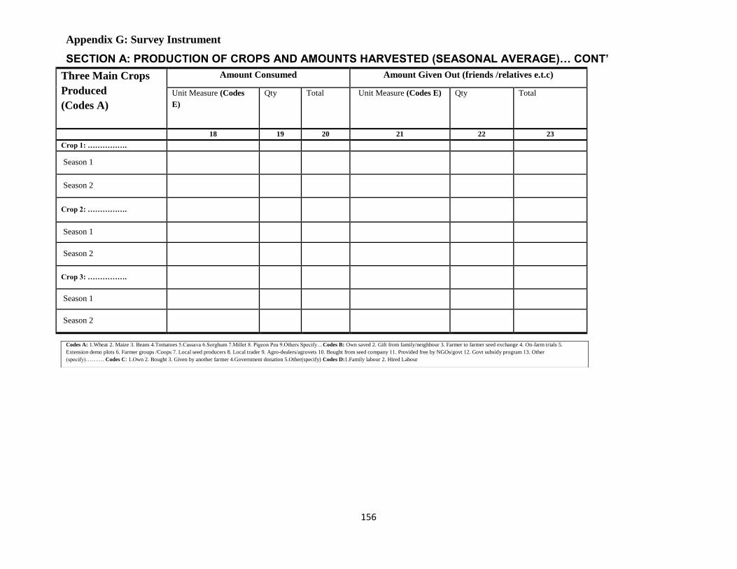
Appendix G: Survey Instrument
156
SECTION A: PRODUCTION OF CROPS AND AMOUNTS HARVESTED (SEASONAL AVERAGE)… CONT’
Three Main Crops
Produced
(Codes A)
Amount Consumed Amount Given Out (friends /relatives e.t.c)
Unit Measure (Codes
E)
Qty
Total
Unit Measure (Codes E) Qty
Total
18 19 20 21 22 23
Crop 1: …………….
Season 1
Season 2
Crop 2: …………….
Season 1
Season 2
Crop 3: …………….
Season 1
Season 2
Codes A: 1.Wheat 2. Maize 3. Beans 4.Tomatoes 5.Cassava 6.Sorghum 7.Millet 8. Pigeon Pea 9.Others Specify…Codes B: Own saved 2. Gift from family/neighbour 3. Farmer to farmer seed exchange 4. On-farm trials 5.
Extension demo plots 6. Farmer groups /Coops 7. Local seed producers 8. Local trader 9. Agro-dealers/agrovets 10. Bought from seed company 11. Provided free by NGOs/govt 12. Govt subsidy program 13. Other
(specify)………. Codes C: 1.Own 2. Bought 3. Given by another farmer 4.Government donation 5.Other(specify) Codes D:1.Family labour 2. Hired Labour
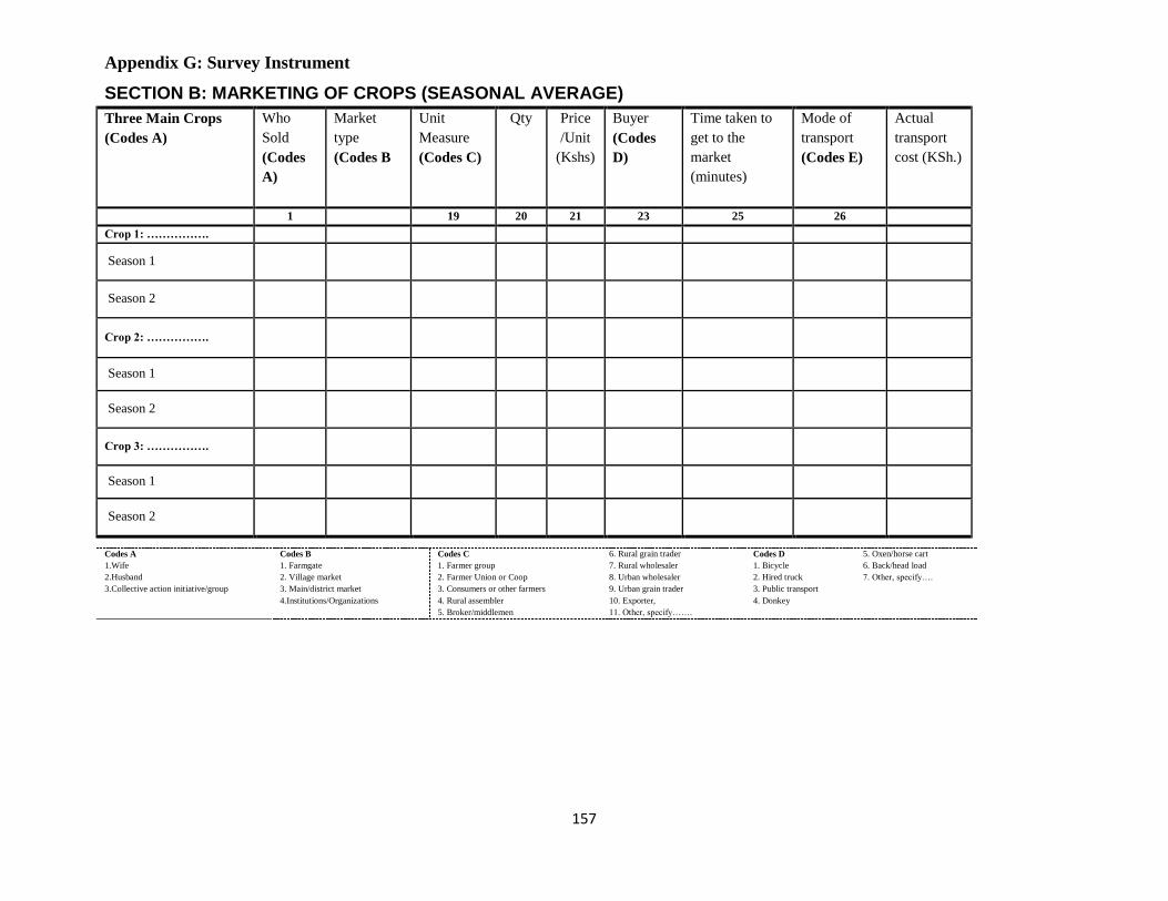
Appendix G: Survey Instrument
157
SECTION B: MARKETING OF CROPS (SEASONAL AVERAGE)
Three Main Crops
(Codes A)
Who
Sold
(Codes
A)
Market
type
(Codes B
Unit
Measure
(Codes C)
Qty
Price
/Unit
(Kshs)
Buyer
(Codes
D)
Time taken to
get to the
market
(minutes)
Mode of
transport
(Codes E)
Actual
transport
cost (KSh.)
1 19 20 21 23 25 26
Crop 1: …………….
Season 1
Season 2
Crop 2: …………….
Season 1
Season 2
Crop 3: …………….
Season 1
Season 2
Codes A
1.Wife
2.Husband
3.Collective action initiative/group
Codes B
1. Farmgate
2. Village market
3. Main/district market
4.Institutions/Organizations
Codes C
1. Farmer group
2. Farmer Union or Coop
3. Consumers or other farmers
4. Rural assembler
5. Broker/middlemen
6. Rural grain trader
7. Rural wholesaler
8. Urban wholesaler
9. Urban grain trader
10. Exporter,
11. Other, specify…….
Codes D
1. Bicycle
2. Hired truck
3. Public transport
4. Donkey
5. Oxen/horse cart
6. Back/head load
7. Other, specify….
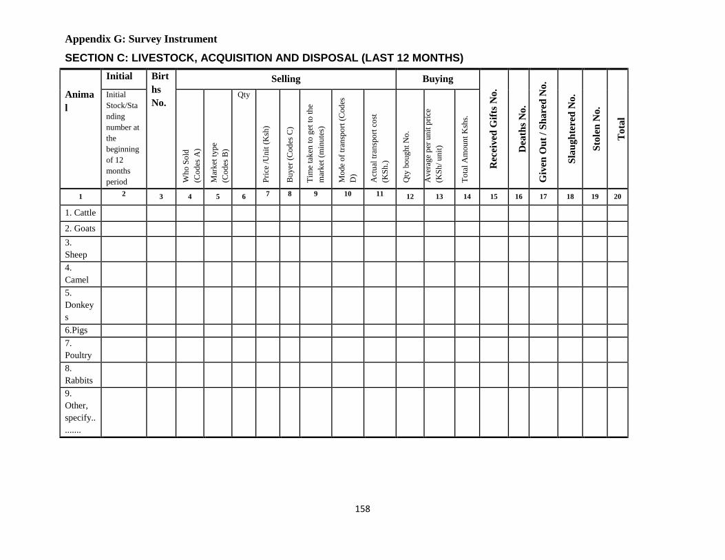
Appendix G: Survey Instrument
158
SECTION C: LIVESTOCK, ACQUISITION AND DISPOSAL (LAST 12 MONTHS)
Anima
l
Initial Birt
hs
No.
Selling Buying
Rec
eived
Gif
ts N
o.
Dea
ths
No.
Giv
en O
ut
/ S
hare
d N
o.
Sla
ugh
tere
d N
o.
Sto
len
No.
Tota
l
Initial
Stock/Sta
nding
number at
the
beginning
of 12
months
period Wh
o S
old
(Co
des
A)
Mar
ket
typ
e
(Co
des
B)
Qty
Pri
ce /
Un
it (
Ksh
)
Bu
yer
(C
od
es C
)
T
ime
tak
en t
o g
et t
o t
he
mar
ket
(m
inu
tes)
Mo
de
of
tran
spo
rt (
Cod
es
D)
Act
ual
tra
nsp
ort
co
st
(KS
h.)
Qty
bo
ug
ht
No
.
Av
erag
e p
er u
nit
pri
ce
(KS
h/
un
it)
To
tal
Am
oun
t K
shs.
1 2 3 4 5 6 7 8 9 10 11 12 13 14 15 16 17 18 19 20
1. Cattle
2. Goats
3.
Sheep
4.
Camel
5.
Donkey
s
6.Pigs
7.
Poultry
8.
Rabbits
9.
Other,
specify..
.......

Appendix G: Survey Instrument
159
SECTION D: LIVESTOCK PRODUCTS: PRODUCTION AND DISPOSAL ACTIVITIES ON A DAILY BASIS (DAILY
AVERAGE)
Type of
Product
Amount Produced Amount
Consumed
Amount
Shared/Gi
ven Out
Amount Sold
Unit
Measure
(Codes
A)
Qty
Tot
al
(L)
Qty
Total
(L)
Qty
Total
(L)
Who
Sold
(Codes
B)
Market
type
(Codes
C)
Qty
Price
/Unit
(Kshs
)
Buye
r
(Cod
es
D)
Time
taken to
get to the
market
(minutes)
Mode
of
transpo
rt
(Codes
E)
Actual
transpo
rt cost
(KSh.)
1 2 4 5 7 8 10 11 12 13 15 16 17 18 19 20
Cattle Milk
1.Dry Season
2. Wet Season
Goats Milk
1.Dry Season
2. Wet Season
Sheep Milk
1.Dry Season
2. Wet Season
Camel Milk
1.Dry Season
2. Wet Season
Codes A
1. Litre
2. 500 ml
3. 250 ml
4. Kilogramme
5. Treetop bottle(750ml)
6. Soda Bottle (300ml)
7. Soda Bottle (500ml)
8. Small Cup (250ml)
9. Headcount
10.Crates
11. Others Specify
Codes B
1.Wife
2.Husband
3.Collective action
initiative/group
Codes C
1. Farmgate
2. Village market
3. Main/district market
4.Institutions/Organizations
Codes D
1. Farmer group
2. Farmer Union or Coop
3. Consumers or other farmers
4. Rural assembler
5. Broker/middlemen
6. Rural grain trader
7. Rural wholesaler
8. Urban wholesaler
9. Urban grain trader
10. Exporter,
11. Other, specify…
Codes E
1. Bicycle
2. Hired truck
3. Public transport
4. Donkey
5. Oxen/
horse cart
6. Back/head
load
7. Other,
specify….

Appendix G: Survey Instrument
160
SECTION E: OTHER LIVESTOCK PRODUCTS: PRODUCTION AND DISPOSAL ACTIVITIES (LAST 12 MONTHS)
Type of
Product
Amount
Produced
Amount
Consumed
Amount Shared
/Given Out
Amount Sold
Unit
Measure
(Codes
A) / No.
Qt
y To
tal
Unit
Measure
(Codes
A)/No.
Q
ty Tota
l
Unit
Measu
re
(Code
s A)
/No.
Qty
Tota
l
Who
Sold
(Codes
B)
Market
type
(Code
s C)
Unit
Measur
e
(Codes
A)/No
Qty
Price
/Unit
(Kshs
)
Buye
r
(Cod
es
D)
Time
taken to
get to the
market
(minutes)
Mode
of
transpo
rt
(Codes
E)
Actual
transp
ort
cost
(KSh.)
1 2 4 5 6 7 8 9 10 11 12 13 14 15 16 17 18 19 20
1. Ghee
2. Eggs
3. Honey
4. Cattle Meat
5. Goat Meat
6. Sheep Meat
7. Cattle
Hides
8. Goat Skin
9. Sheep Skin
10. Camel
Hides
11. Others,
Specify
Codes A
1. Litre
2. 500 ml
3. 250 ml
4. Kilogramme
5. Treetop bottle (750ml)
6. Soda Bottle (300ml)
7. Soda Bottle (500ml)
8. Small Cup (250ml)
9. Headcount
10.Crates
11. Others Specify
Codes B
1.Wife
2.Husband
3.Collective action
initiative/group
Codes C
1. Farmgate
2. Village market
3. Main/district market
4.Institutions/Organizations
Codes D
1. Farmer group
2. Farmer Union or Coop
3. Consumers or other farmers
4. Rural assembler
5. Broker/middlemen
6. Rural grain trader
7. Rural wholesaler
8. Urban wholesaler
9. Urban grain trader
10. Exporter,
11. Other, specify…….
Codes E
1. Bicycle
2. Hired truck
3. Public transport
4. Donkey
5. Oxen/horse cart
6. Back/head load
7. Other,
specify….

Appendix G: Survey Instrument
161
PART 6: TRANSFER AND OTHER SOURCES OF INCOME DURING (LAST 12 MONTHS)
Sources
Who earned/ received?
0= None;
1=Women 2=Men;
3=Both
No. of units
worked/
received( days,
weeks, months,
years)
Amount per unit (Cash &
in-kind)
Total income (cash & in-
kind) Total
income
(KSh) Cash
(KSh)
Payment in
kind Cash
equivalent
Cash
(KSh)
Payment in
kind Cash
equivalent
1 2 3 4 5 6= 3x4 7=3x5 8= 6+7
1. Leased Parcel
2. Selling Firewood
3. Selling Charcoal
4.Sale of crop residues
5.Sale of fish/fish farming
6.Sale of hay
7.Sale of dung
8.Farm Labour wages
9.Non-farm labour wages
10. Non-farm business
11. Drought/flood relief
12.Safety net or food for work
13. Remittances (sent from non-
resident family and relatives living
elsewhere)
14. Other, specify
PART 7: ACCESS TO FINANCIAL CAPITAL, INFORMATION AND EXTENSION
SECTION A: INFORMATION AND EXTENSION
1. Do you have access to extension services? (1.yes; 2. No)…………………………………………………….
2. If yes, fill in the table below

Appendix G: Survey Instrument
162
Issue
Three main
items/issues that you
received
training/information
on […...] during the
last 12 months
(1=most important)
Main information
source, Rank 3
(Codes A)
Main type of
extension approach
used, Rank 3
(Codes B)
Number of
contacts
during the
last 12
months
(days/year)
Household
perception
on the
quality of
information
(Codes C) 1st 2nd 3rd 1st 2nd 3rd
1 2 3 4 5 6 7 8 9 10
1. New varieties of fodder crops
2. New varieties of crops
3. Field pest and disease control
4. Trees/tree management/agro-forestry
5. Soil and water conservation
6. Minimum tillage
7. Leaving crop residue in the field
8. Adaptation to climate change
9.Information on destocking
10. Crop storage pests
11. Output markets and prices
12. Input markets and prices
13. Collective action/farmer organization
14. Livestock production (new breeds;
indigenous breeds e.t.c)
15.Information on livestock-crop integration
16. Others, specify…………..
Codes A
1. Government extension service
2. Farmer Coop or groups
3. Neighbour farmers
4. Seed traders/Agrovets
5. Relative farmers
6. NGOs
7. Other private trader
8. Private Company
9. Research centres
10. Farmers Field Schools (FFS)
11. Faith-Based Organizations (FBOs)
12. Community-Based Organisations (CBOs)
13. Other, specify……
Codes B
1. Farm visits
2. Farmer research groups seminars/talks
3. Farmer field schools
4. Farmer-to-farmer exchange visits
5. Mobile phone
6. Radio/TV
7. Newspaper
8.Other ,specify……….
Codes C
1= Very poor
2= Poor
3= Average;
4=Good
5= Very good

Appendix G: Survey Instrument
163
3. Do you own a mobile phone? (1.yes; 2. No)…………………………………………………….………………
4. If yes, how often to do you use it to receive extension information? (1. Often; 2. Rarely; 3. Never)……………
SECTION B: ACCESS TO FINANCIAL CAPITAL, HOUSEHOLD CREDIT NEED AND SOURCES (LAST 12 MONTHS)
Expense Item
Rank the three
main needs of
finance (codes
A)
Amo
unt in
local
curre
ncy
Need
ed
credit
?
(Cod
es B)
If Yes
in
column
6, then
did you
get it?
(Codes
B)
If No in column
7, then why not?
Rank 3 (codes
C)
If Yes in column 7
1st 2n
d
3r
d 1st
2n
d 3rd
Source
of
Credit,
(Codes
D)
How
much did
you get
(KSh)
Did you get
the amount
you
requested
(Codes B)
Annual
interest
rate
charged
(%)
1 2 3 4 5 6 7 8 9 10 11 12 13 14
1. Buying seeds (per year) 2. Buying fertilizer(per year)
3. Buy herbicide and pesticides (per year)
4. Buy farm equipment/implements (per
year)
5. Buy oxen for traction(per year)
6. Buy other livestock (per year)
7. Invest in irrigation system(per year)
8.. Non-farm business or trade(per year)
9. To pay land rent(per year)
10. Buy food
11.Transport costs (per month)
12.Electricity (per moth)
13.Water (per month)
14.Cooking fuel (per month)
15.Education (per year)
16.Health care (per year)
17.Entertainment (per year) 18. Other Consumption needs (exclusive
of the consumption needs listed above)
ones listed above)
Codes A
1. Own Farm Income 2. Own Non –farm Income
3. Income from farmer groups’ microenterprise
initiatives
4. Income from
conservancies
5. Credit
Codes
B
0. No
1. Yes
Codes C
1. Interest rate was high 2. Too much
paper work/ procedures 3. I have no asset
for collateral
4. No money lenders in this area for
this purpose 5. Lenders don’t
provide the amount needed6. Other,
specify..
Codes D
1.Farmer group
2. Money lender
3. Microfinance, 4. Bank
5. SACCO Loan
6. Relative/Friends
7. AFC 8..Merry go rounds,
9. Other, specify..

Appendix G: Survey Instrument
164
SECTION C: HOUSEHOLD FINANCIAL NEEDS FOR FOOD CONSUMPTION
5. Household food consumption financial needs (last month)
Product
Consumed
amount per
month
Unit
Kg/litres Price per unit
Meat
Rice
Wheat Flour
Bread
Maize Flour
Cooking Oil
Eggs
Sugar
Butter
Potato
Carrot
Onion
Cassava
Cabbages/Sukuma
wiki/Spinach
Other Vegetables
Fruits
Alcohol and tobacco
Other (specify)
“___________”

Appendix G: Survey Instrument
165
SECTION D: HOUSEHOLD SAVINGS
PART 8: RISK, LIVELIHOOD SHOCKS AND COPING STRATEGIES
1. Have you noticed any long-term changes in temperature over the last 10 years? (1. Increased, 2. Decreased, 3. Stayed the same,
4. Don‘t know)……….
2. Have you noticed any long-term changes in rainfall over the last 10 years? (1. Increased, 2. Decreased, 3. Stayed the same, 4.
Don‘t know)..
3. Have you noticed any long term changes in rainfall patterns /variability over the last 10 years? (1. Yes, 2. No 3. Don‘t know)…..
4. Have you noticed any other changes in climate over the last 10 years?(1=yes, 2=no)….. If yes, please specify………
5. Further questions on risk, livelihood shocks and coping strategies.
Name of Saving
family member
Relation to HH
head
Has bank account
(0=No; 1=Yes)
Saving with
(Codes A)
Range of Total amount saved during the
last 12 months (KSh) (Codes B)
1 2 3 5
Codes A
1. Saving at home (personal)
2. Commercial or other banks
3. Rural micro-finance
4. SACCO (credit society)
5. Merry go-round
6. Mobile phone banking (e.g. M-Pesa)
7. Saving by lending to money lender
8. Other, specify………….…
Codes B
1. Zero/None
1.1-5,000K shs
2. 5,001-10,000 Kshs
3. 10,001-20,000 Kshs
4. 20,001-50,000
5.>50,000

Appendix G: Survey Instrument
166
Risk factor
Rank three
important
risk
factors[…]
affecting
household
livelihood
(1=most
important)
Important coping
strategies
before/after
occurrence
(mitigation/adapta
tion) […],
Codes A; Rank 3
How did
[…] affect
production
of main
food crop of
the
household
(%
reduction)
As a result
of […] did
you lose
(part of)
your income
(%
reduction)
Do you think
[…] will
become more
important in
future due to
climate
change
Codes B
If Yes,
how
often do
you think
[…] will
occur in
the next
ten
years? 1
st 2
nd 3
rd
1 2 3 4 5 9 10 11 12
1. Drought
2. Too much rain or floods
3. Inadequate water harvesting facilities
4.Crop pets/diseases
5. Livestock diseases or death of livestock
6.Declining grazing pastoral areas
7. Large decrease in crop output prices
8. Large decreases in livestock output prices
9. Large increases in crop input prices
10. Large increases in livestock input prices
11. Large increase in food prices
12. Theft of assets or livestock
13. Reduced/failure household business income
14. Reduced/loss of employment income
15. Conflict
16. Others (Specify)………….
Codes A
1. Re-aggregation of parcels of land
2.Selling of livestock
3. Herd splitting
4. Changing livestock species
5. Planting drought tolerant
pastures
6.Plant disease/pest tolerant
Crop varieties
7. Crop diversification
8. Out Migration
9.Soil and water conservation
10. None
11. Planting drought tolerant crops
12. Leasing land
13. Selling land
14. Sale of charcoal
15. Selling livestock
16.Replanting
17. Selling other assets
18.Eat less (reduce meals)
19. Sale of firewood
20. Borrowing
21. Casual labour
22.Petty trade
23. Out-Migration
24.Dietary changes
25. Other, specify..
Codes B
0. No
1. Yes

Appendix G: Survey Instrument
167
PART 9: HOUSEHOLD ASSET OWNERSHIP AS A WELFARE INDICATOR
1. Indicate the ASSETS that the household owns at the moment.
Notes:
1. Main walling material of main residential house (CodesA)…………….………………………......................................
2. Main roofing material of main residential house (CodesB)………………………………… ……………………………
3. Type of toilet used (Codes C)............................................................................................................................................................
Codes A
1. Burned bricks
2. Unburned bricks
3. Stone
4. Earth
5. Wooden (timber)
6. Other, specify……
Codes B
1. Grass thatch
2. Iron sheet
3. Tiles
4. Other, specify……
Codes C
1. Flush toilet private
2. Flush toilet shared
3. Pit latrine private
4. Pit latrine shared
5. Bucket latrine
6. No toilet/use open air
ENDING TIME............................
Current Total Current Total
Number Unit current Number Unit current
Item value value Item value value
Cow shed (s) Solar panel
Ox plough Irrigation equipment
Food store Generator
Refrigerator Sewing machine
Well (water well) Farm house(s) (see notes 1 and 2 below)
Milking shed Toilet ( see note 3 below)
Water tank Panga
Water pump Jembe
Water trough Vehicle(s)
Milking shed Tractor
Feed troughs Tractor trailer
Wheel barrow Motorbike
Donkey/ox cart Mobile phone
Bicycle Fixed land line
Television Electricity (access & wired from station)
Radio Batteries
Spade/shovel