zimora – an atmospheric dispersion model · 2014-05-12 · zimora – an atmospheric dispersion...

ZIMORA – an atmospheric dispersion model

H. R. Zimermann & O. L. L. Moraes Laboratório de Micrometeorologia, CRS/INPE – Universidade Federal de Santa Maria, Brazil

Abstract

This paper presents a development and validation of a 3D numerical model for the advection-diffusion equation. Atmospheric flow field generated by mesoscale circulation model is used as input for the wind speed. As the mesoscale model gives information at scale higher than the necessary for description of a plume trajectory a weighted linear average proper interpolation was developed for intermediate these distances. Diffusion coefficients are variables in time and space and are different for lateral and vertical directions. This assumption is important and considers that the turbulence is not isotropic. Numerical scheme is explicit and conservative and has small implicit diffusion in the advection part of the model. Boundary conditions are open at lateral domain and normal in the bottom and at the top of the Planetary Boundary Layer (PBL) height. Output of the model can be viewed at any time step as well as the concentration distributions are showed at horizontal or vertical surfaces. For validation of the model two experiments were carried out near a thermoelectric power plant located in the south of Brazil. Each experiment was forty days longer. Hourly SO2 concentrations were collected in four receptors around the power plant. During the experiments micrometeorological measurements and tethered balloons were also used in order to describe properly the local atmospheric circulation and PBL characteristics. Various static indices indicate that the model works very well at least for the source and the terrain were it is located, i.e. continuous emission and homogeneous topography. Keywords: data assimilation, numerical 3D model, atmospheric pollutant dispersion, Zimora, finite differences scheme, K-theory.

Air Pollution XVII 63

www.witpress.com, ISSN 1743-3541 (on-line)

© 2009 WIT PressWIT Transactions on Ecology and the Environment, Vol 123,

doi:10.2495/AIR090061

1 Introduction

One of the most challenging and widespread environmental problems facing the international community today is air pollution. Both the monitoring and modelling of air pollution is essential to provide a picture of the damage humans are doing to the environment, and to enable pollution problems to be discovered and dealt with. The main idea of a model is to describe what may happen to pollutant once it enters the surrounding atmosphere, where it goes and how it is diluted. In general the mathematical description of this process is done by eulerian or lagrangian models. Understanding the distribution and fluxes of various atmospheric trace constituents requires a proper knowledge of atmospheric transport as well as the relevant physical and chemical transformation and deposition processes for the trace species considered. Numerical modelling currently presents a powerful way of analyzing many problems related to the atmospheric trace constituents. The increasing power of digital computers as well as a steady improvement in the quality and resolution of meteorological data has led to the development and successful application of three-dimensional atmospheric transport models on a range of scales from local to global. In this paper it is presented the development and evaluation of numerical model, Zimora that solves the advection-diffusion equation. The Zimora is and Eulerian based model since it treats conservative equations. It achieves meteorological fields by the use of a dynamical class meteorological pre-processor model (to hereafter MPP) output. In its actual development stage it acquires only wind velocity to numerically solve the prognostic advection-diffusion equation. The dynamical mesoscale numerical model output, used as input into Zimora, for wind field was the Brazilian version of the Regional Atmospheric Modeling System (CSU-RAMS) developed by Colorado State University (USA) and adapted for Brazilian purposes and known by the name BRAMS. Its actual operational status, running as the main weather forecast product from the Atmospheric Modeling Group (GRUMA) facilities in the Santa Maria Federal University, centre of southern state in Brazil, has an output resolution of 3 hours for the time scale and 20 kilometres for horizontal scales and 17 vertical geopotential levels. The proper fields downscaling for input into Zimora will be discussed in details in the 2.1 section.

2 Description of the model

The prognostic equation adopted by this model is based in the physical principles of mass conservation representing the continuity of atmospheric fluid air parcel. This equation, in the general major of the mathematical treatments of diffusion from point sources, is the differential equation that has been used as start point, is a generalization of the classic equation of heat transference in solids, in heat form, by conduction and is essentially one description of mass conservations of the suspended material (Slade [27]). Consider for example, any scalar concentration quantity C , we express the conservation equation by:

64 Air Pollution XVII



.).( DSCVtC

+=∇+∂∂ (1)

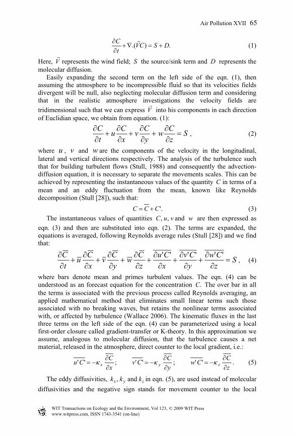
Here, V represents the wind field; S the source/sink term and D represents the molecular diffusion. Easily expanding the second term on the left side of the eqn. (1), then assuming the atmosphere to be incompressible fluid so that its velocities fields divergent will be null, also neglecting molecular diffusion term and considering that in the realistic atmosphere investigations the velocity fields are tridimensional such that we can express V into his components in each direction of Euclidian space, we obtain from equation. (1):

SzCw

yCv

xCu

tC

=∂∂

+∂∂

+∂∂

+∂∂

, (2)

where u , v and w are the components of the velocity in the longitudinal, lateral and vertical directions respectively. The analysis of the turbulence such that for building turbulent flows (Stull, 1988) and consequently the advection-diffusion equation, it is necessary to separate the movements scales. This can be achieved by representing the instantaneous values of the quantity C in terms of a mean and an eddy fluctuation from the mean, known like Reynolds decomposition (Stull [28]), such that:

'.CCC += (3) The instantaneous values of quantities vuC ,, and w are then expressed as eqn. (3) and then are substituted into eqn. (2). The terms are expanded, the equations is averaged, following Reynolds average rules (Stull [28]) and we find that:

SzCw

yCv

xCu

zCw

yCv

xCu

tC

=∂

∂+

∂∂

+∂

∂+

∂∂

+∂∂

+∂∂

+∂∂ ''''''

, (4)

where bars denote mean and primes turbulent values. The eqn. (4) can be understood as an forecast equation for the concentration .C The over bar in all the terms is associated with the previous process called Reynolds averaging, an applied mathematical method that eliminates small linear terms such those associated with no breaking waves, but retains the nonlinear terms associated with, or affected by turbulence (Wallace 2006). The kinematic fluxes in the last three terms on the left side of the eqn. (4) can be parameterized using a local first-order closure called gradient-transfer or K-theory. In this approximation we assume, analogous to molecular diffusion, that the turbulence causes a net material, released in the atmosphere, direct counter to the local gradient, i.e.:

.'';'';''zCCw

yCCv

xCCu zyx ∂

∂−=

∂∂

−=∂∂

−= κκκ (5)

The eddy diffusivities, zyx kkk and, in eqn. (5), are used instead of molecular diffusivities and the negative sign stands for movement counter to the local




gradient. The set of equations, eqn. (5), are then respectively substituted into last three terms on the left side of the eqn. (4). The terms are expanded using associative properties of the derivative operator and we find that:

.2

2

2

2

2

2

SzC

zC

zyC

yC

y

xC

xC

xzCw

yCv

xCu

tC

zz

yy

xx

=∂∂

−∂∂

∂∂

−∂∂

−∂∂

∂

∂−

+∂∂

−∂∂

∂∂

−∂∂

+∂∂

+∂∂

+∂∂

κκκκ

κκ

(6)

The eqn. (6) is the equation of tridimensional advection-diffusion time independent for non isotropic, zyx kkk and, are variable in space and time, turbulence and with source presence. This equation is evaluated using the Lax-Wendroff one-step explicit method, which consists of the approximation for convection equation using Taylor series expansion and second-order, centered-difference, finite difference approximations techniques (Lax-Wendroff, 1960). The time derivative tC ∂∂ is then evaluated and their respective three dimensional fields are projected forward through a short time step tδ . The diagnostic equations are then applied to obtain dynamically consistent fields of the other dependent variables at time tt δ+0 . The process is then repeated over succession of time steps to describe the evolution of the .C The time step tδ must be short enough to ensure that the fields of the dependent variables are not corrupted by spurious small scale patterns arising from numerical instabilities. The higher the spatial resolution of the model, the shorter the maximum allowable time step and the larger the number calculations are required for each individual time step (Wallace, 2006). The numerical equation to be solved is:

( ) ( ) ( )

( )( ) ( )( )

( )( ) ( )( ) ( ).22

241

41

41

21

21

21

1,,,,1,,2,1,,,,1,2

,,1,,,,121,,1,,1,,1,,

,1,,1,,1,,1,,,1,,1,,1,,1

1,,1,,,1,,1,,,1,,1

,,,,1,,

nkji

nkji

nkjiz

nkji

nkji

nkjiy

nkji

nkji

nkjix

nkji

nkji

nkji

nkji

nkji

nkji

nkji

nkji

nkji

nkji

nkji

nkji

nkji

nkji

nkji

nkji

nkji

nkji

kjin

kjin

kji

CCCztKCCC

ytK

CCCxtKCCKK

zt

CCKKytCCKK

xt

CCztwCC

ytvCC

xtu

SCC

−+−+

−+−+−+

−+−+−+−+

−+−+−+

+

+−∆∆

+++−∆∆

+

++−∆

∆+−−

∆∆

+

+−−∆∆

+−−∆∆

+

+−∆∆

−−∆∆

−−∆∆

−

++=

(7)

To avoid this computational instability, we use the Courant Friederichs-Levy (CFL) stability condition limited to values lower than 0.8:

.8.0CFL,8.0CFL 2 ≤=≤=itK

itU idiffiadv δ

δδδ (8)

In eqn. (8) the subscripts i ( 3,2,1=i ) represents the components of the wind velocity and diffusivities coefficients in the longitudinal, lateral and vertical directions respectively. The initial source condition for Zimora is a puff release characterized by a Gaussian shape distribution of matter given by (Lyons 1990):




( ) ( ) .41exp

4,,,,,,

222

3

++−=

ssssss z

s

y

s

x

s

zyx

ssssss K

zKy

Kx

tKKKtzyxtSzyxtC

π (9)

In eqn. (9) the subscripts s referrers to the coordinates point of the source location. The remaining continuous release of the matter is represented as sequences of this puff by instantaneous releases from the source. Assuming the domain like a box, the boundary conditions are normal in the bottom and at the top of the PBL height:

,0;;00 =∂∂

⇒==∨=zCKzzzk ziz (10)

and they are open at lateral domain:

.),,,1(),,,(t

zyxtCVt

zyxtC∂−∂

−=∂

∂ (11)

2.1 Downscaling the wind field

The Zimora seeks to model the atmospheric dispersion with higher spatial resolution than his MPP provides. Hence we developed a multi layer scheme constructed using simple linear weighted average proper to downscale the low spatial resolution of the MPP into any multiple linear spatial scale. To figure out, let’s use one dimensional case for simplicity; using two points A and B, representing two known values of any scalar quantity, spaced by a distance D kilometres between them, representing the low resolution. We want to downscale this last to a new high resolution by d kilometre. We evaluate any new point between them using weighted average techniques, attributing to A and B specific weight in each subinterval (D/d) in the new scale between A and B and use weight average. The mathematical expression for weight average is given by:

∑∑==

=m

ii

m

iiin wwxx

11, (12)

where ix is the generator entity (A or B values), m is the numbers of points of

known values, two in this example (A and B), being averaged and iw is its weight associated to each interval where we desire evaluate. To determine the weights of A and B, as our example, we need two suppositions: a) At the point of view of A, its weight should contribute the most at his own point and in the B point should be null; b) At the point of view of B the rule is the same, weight of B is maximum in his own point and null in the A point. After that, we can guess mathematical expressions that agrees these suppositions and plays transference function role to the weights of A and B, such mathematically does not alters the values of A and B and allows interpolation between them. Generalizing for 4 known points UA,UB,UC and UD, equally spaced, like figure (1), we found these expressions:

,)),max((*1, jip

xH AU

ji −=δ

(13)




,)),min((*11,

−−= jip

xH DU

ji δ (14) ,,1,

DB Ujip

Uji HH −+=

(15) .,,

BC Uij

Uji HH =

(16) In the set of equations (13-16) the ji, represents the grid node in the new scale which we are building, xδ is the spatial scale factor that we are reducing from the initial grid, 1+= xp δ and H represents the weight function respective for its superscript known point in each new grid node. So, the set of equations

(13-16) plays the role of iw into a generalized two-dimensional form of the eqn. (12). The Zimora model assimilates the wind and turbulent diffusivities coefficients fields, with resolution of 20 km, from the output of the MPP; after that it increase those resolutions to 5 km. The fig. 1 shows the Zimora’s non-staggered grid where the four black nodes represents the MPP output and the grey nodes represents the new resolution with unknown values to be interpolated for that field.

Figure 1: Example of non-staggered grid with four known points (black) and unknown points (grey).

Using the figure 1, example of data input scheme for Zimora model from mesoscale forecast model for the wind velocity, we can demonstrate a practical example. Let us assume that the velocities in the corners are (UA=3.629, UB=3.630, UC=4.025 and UD=3.994) for wind field in the 20 km spatial resolution from MPP output. In order to evaluate Zamora’s’ grey unknown points with spatial resolution of 5 km non-staggered grid, we first find the spatial

UA

UC

UB

UD




resolution factor .4520 == kmkmxδ Then, applying this into the set of eqn. (13-16) and letting the ji, vary for 1=p to 1+= xp δ , we get 1−p elements of

a matrix ppH x~ . Calling each of these layers and using into a generalized two

dimensional form of the equation (12):

,

1

1

∑

∑

=

== m

k

k

m

k

kk

ij

ij

ij

H

HUZ (17)

here, the index k represents each one of known points UA,UB,UC and UD, and evaluating for ji, ranging from 1=p to 1+= xp δ , we get a 5x5

~Z matrix which represents the Zimora new nodes values as shown in table 1.

Table 1: Values of the final 5x5~Z downscaled wind field in the new

resolution non-staggered grid by interpolation using weight layers.

3.629 3.629 3.630 3.630 3.630 3.728 3.756 3.756 3.757 3.721 3.827 3.822 3.820 3.817 3.812 3.926 3.888 3.883 3.878 3.903 4.025 4.017 4.010 4.002 3.994

This same procedure is applied, repeated, until the last MPP output grid points, always in groups of four nodes. Generalizations are the same for vertical, changing only the spatial resolutions both in MPP output and Zamora’s’ grid points, such in the final process we construct volumetric cells of 5km x 5km x 100m.

3 The boundary layer parameterizations

In order to evaluate the diffusion coefficients that are in numerical equation, we have used the boundary layer parameterization proposed by Moraes [22]. This parameterization is based on Hanna [4] assumption that the mixing efficiency of the air is completely determined by the properties of the vertical velocity spectrum, and that the parameters, vertical dispersion parameter wσ , and mk are sufficient to describe the vertical velocity spectrum. Then it follows from dimensional reasoning that the vertical eddy diffusivity coefficient zK may be written as

-1m1 kwz cK σ= (18)

where 1c is a constant equal to 0.09. From the measurements done in the surface layer and using local scalings assumptions we obtained for the vertical turbulent diffusion coefficient in the




whole boundary layer the following expressions for stable and convective atmospheric stability regimes

,)/1)(/(50.027.0

)/1)(/(1)/1(

12

121

5.1

5.12/

*1 αα

ααα

−

−

−+

−+−=

hzLzhzLzhzzucK z (19)

),/1(5.0 * iz zzzwK −= (20) where z is the height above ground, iz is the boundary layer height, *u is the friction velocity, 1α and 2α are constants determined experimentally (Moraes et. al. 1991; Moraes [22]), L is the local Monin-Obukhov length and *w is the vertical convective scale. The lateral diffusion coefficient is estimated as izw*1.0 in unstable conditions and as MzK2 in neutral-stable conditions, where MzK is the maximum of zK .

4 Verification of Zimora against experimental data results

In order to test and validate the model a micrometeorological experiment was conducted in the 2007 spring season near a thermoelectric power plant located in the Candiota town, south of Brazil near Uruguay border. This power plant can be considered an ideal Laboratory since it is the major source of some pollutants in a large area and it is located in a region of smooth topography. The power plant has a 150-m height stack and the rate of emission of e.g. SO2 is continuously monitored. The objective of the campaign was to collect a comprehensive, meteorological diffusion and dispersion database to be used to evaluate the dispersion numerical model. The campaign site (31.40S, 53.70W, 250 m above sea level) has previously been used for a number of experiments related to research on atmospheric boundary layer (for details and results from the micrometeorological point of view see Moraes [22]). It is located in a region known as the South America (SA) Pampa. The Pampa is the part of SA that covers all Uruguay territory, the south of Brazil and northwest of Argentina Meteorological data was collected over a 5-week time resulting in a full set of daytime period and the database comprises measurements of wind speed, wind direction, turbulence, temperature, humidity, pressure, solar radiation, the boundary layer structure and upper-air-soundings. The data records were broken into 1-hr segments and those collected at 10 Hz were used to compute micrometeorological parameters ( ∗u , ∗w , L ) and data collected at 1 Hz were used to estimate wind speed, wind direction and air temperature. Tethered balloon was launched each two hours and gives information mainly of the evolution of the PBL height. Ground level concentrations, used in this paper, were measured in one position located 6.8 km to the southwest of the source. The concentration data set consists of three hours values of SO2. Figure 2 and 3 below as well as table 2 presents the model performance. Figure 2 is an example of the SO2 plume evolution for one day of simulation. Each panel has the hourly mean concentration for some specific hours of the day. The selected day choose for this presentation was characterized by a cold front




Figure 2: From left to right and top to bottom, 1, 4, 8, 12, 16 and 20 hours SO2 plume time evolution simulated for the day 27/09/2008. The concentrations in the bar scale are µg / m3 and wind speed scale is m/s which magnitude scale is shown by the arrow over number on the bottom corner of each graph.

that passed in the region and we can see that the model represents very well the change of the wind direction due this cold front. To avoid some misunderstanding, due to the gray scale shaded allowed by data visualization software, as far from the center point the shaded contour refers for the leftmost concentrations values in the bottom scale. Figure 3 is the comparison between model prediction and observations of SO2 ground concentration. Table 2 presents some statistical indices, defined as the




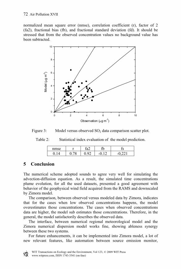
normalized mean square error (nmse), correlation coefficient (r), factor of 2 (fa2), fractional bias (fb), and fractional standard deviation (fd). It should be stressed that from the observed concentration values no background value has been subtracted.

0 2 4 6 8 100

2

4

6

8

10M

odel

(µg

m-3)

Observation (µg m-3)

Figure 3: Model versus observed SO2 data comparison scatter plot.

Table 2: Statistical index evaluation of the model prediction.

nmse r fa2 fb fs 0.14 0.78 0.92 -0.12 -0,221

5 Conclusion

The numerical scheme adopted sounds to agree very well for simulating the advection-diffusion equation. As a result, the simulated time concentrations plume evolution, for all the used datasets, presented a good agreement with behavior of the geophysical wind field acquired from the RAMS and downscaled by Zimora model. The comparison, between observed versus modeled data by Zimora, indicates that for the cases when low observed concentrations happens, the model overestimates those concentrations. The cases when observed concentrations data are higher, the model sub estimates those concentrations. Therefore, in the general, the model satisfactorily describes the observed data. The interface, between numerical regional meteorological model and the Zimora numerical dispersion model works fine, showing ableness synergy between these two systems. For future enhancements, it can be implemented into Zimora model, a lot of new relevant features, like automation between source emission monitor,




enhance the parameterizations and development of graphical interfaces to uses it as air quality monitor and virtual research lab.

Acknowledgements

This work was supported by the Companhia de Geração Térmica de Energia Elétrica (CGTEE) and by the Brasilian Agency for the Development of Science and Technology (CNPq).

References

[1] Barnes, L. S.: 1964,A Technique for maximizing Details in Numerical Weather Map Analysis, Journal of Applied Meteorology, Vol. 3, 396-409.

[2] Bendat, J. S., Piersol, A. G.:1990, Random Data - Analysis And Measurement Procedures, 2nd Ed., Wiley, New York.

[3] Cressman, G. P.:1959,An Operational Objective Analysis System, Monthly Weather Review. 87, 367-374.

[4] Hanna, S. R.:1968, A method of estimating vertical eddy transport in the planetary boundary layer using characteristics of the vertical velocity spectrum., Journal of Atmospheric Sciences, Boston, Vol. 25,1026.

[5] Haugen, D. A.:1978,Effects os sampling rates and averaging periods on meteorological measurements., In. Proc. Fourth Symposium on Meteorological Observations and Instrumentation, April 1978, Denver, CO, American Meteorological Society, Boston, MA, 15-18.

[6] Hibbard, W. L., Wylie, D. P.:1985,An Efficient Method of Interpolating Observations to Uniformly Spaced Grids., Conf. Interactive Information and Processing systems (IIPS) for Meteorology, Oceanography and Hydrology.

[7] Hinze, J. O.:1975, Turbulence., McGraw-Hill. [8] Jesus, S.M.:1999/00, Estimação Espectral e Aplicações,Curso: Engenharia

de Sistemas e Computação,Faculdade de Ciências e Tecnologia, University of Algarve.

[9] Hoffman, J. D.. 1993. Numerical Methods for Engineers and Scientists. Mechanical Engineering Series, McGraw- Hill International Editions.

[10] Kaimal, J. C and Finnigan, J. J.:1994, Atmospheric Boundary Layer Flows: Their Structure and Measurements, Oxford Press. 289pp.

[11] Kovalets, I. V., Tsiouti, V., Andropoulos, S., Bartzis, J. G.:2008, Improvement of Source and Wind Field Input of Atmospheric Dispersion Model by Assimilation of Concentration Measurements: Method and Applications in Idealized Settings, Applied Mathematical Modelling, In Press.

[12] Lamb R. G. (1978). A numerical simulation of dispersion from an elevated point source in the convective boundary layer. Atmospheric Environment 12, 12971304

[13] Lax, P.D., Weak solutions of nonlinear hyperbolic equations and the numerical computation, Comm. Pure Appl. Math.7 (1954), 159-193.




[14] Lax, P.D., Hyperbolic systems of conservation laws II, Comm. Pure Appl. Math., 10 (1957), 537-566.

[15] Lax, P. D., and Wendroff, B. (1960). Systems of conservation laws. Commun. Pure Appl. Math. 13, 217-237.

[16] Lin, C. C.:1953, On Taylor’s Hypothesis and the Acceleration terms in the Navier-Stokes Equation., Quarterly Applied Math., 10:295

[17] Lin, C. C; Reid, W.H.:1963, Handbuc der Physic., volume VIII/2, chapter Turbulent Flow. Theoretical Aspects., Springer-Verlag, 438-523.

[18] Lisieur, M.: 1997,Turbulence In Fluids, 3rd Ed., Kluwer Academic Publishers, Dordrecht.

[19] Lumley, J. L., Panofsky, H. A.: 1964,The Structure Of Atmospheric Turbulence, John Wiley & Sons, London, 232pp.

[20] Lyons, T. J. and Scott, W. D.: 1990, Principles of Air Pollution Meteorology, Belhaven Press, 22pp.

[21] Moraes O. L. L., R. C. M. Alves, R. Silva, A. C. Siqueira, P. D. Borges, T. Tirabassi, U. Rizza. 2001 25th NATO/CCMS International Technical Meeting on Air Pollution Modeling and its Application, Louvain-la-Neuve 15-19, Belgium, p. 359.

[22] _____.:2000. Turbulence Characteristics In The Surface Boundary Layer Over The South American Pampa. Boundary-Layer Meteorology 96: 317-335.

[23] _____., Ferro, M., Alves, R.C.M., and Tirabassi, T 1998.Estimating eddy diffusivities coefficients from spectra of turbulence. Air Pollution, v. VI, p. 57-65.

[24] _____., Degrazia, G.A., and Tirabassi, T. 1998 Using the Prandtl-Kolmogorov relationship and spectral modeling to derive an expression for the eddy diffusivity coefficient for the stable boundary layer. IL Nouvo Cimento, v. 20D, n. 6, p. 791-798.

[25] Panofsky, H. A.:1949,Objective Weather Map Analysis, Journal of Meteorology, No. 6, Vol. 6, 386-392.

[26] Seaman, L. N.:2000, Meteorological Modeling for Air-Quality Assessments, Atmospheric Environment, N. 34, 2231-2259.

[27] Slade, D. H.:1968, Meteorology and Atomic Energy-1968, USAEC, TID-24190, 445pp.

[28] Stull, R. B.:1988, An Introduction to Boundary Layer Meteorology, Kluwer Academic, 637pp




zimora – an atmospheric dispersion model · 2014-05-12 · zimora – an atmospheric dispersion...

Documents