ZNN DocumentationRelease 0.1.2

Aleksandar Zlateski; Kisuk Lee; Jingpeng Wu; Nicholas Turner;

October 20, 2016

Contents

1 Introduction 31.1 When to Use ZNN . . . . . . . . . . . . . . . . . . . . . . . . . . . . . . . . . . . . . . . . . . . . 31.2 CPU vs GPU? . . . . . . . . . . . . . . . . . . . . . . . . . . . . . . . . . . . . . . . . . . . . . . 31.3 What do I need to use ZNN? . . . . . . . . . . . . . . . . . . . . . . . . . . . . . . . . . . . . . . . 41.4 Resources . . . . . . . . . . . . . . . . . . . . . . . . . . . . . . . . . . . . . . . . . . . . . . . . . 41.5 Publications . . . . . . . . . . . . . . . . . . . . . . . . . . . . . . . . . . . . . . . . . . . . . . . 4

2 Installation 52.1 Using Docker image - Recommended . . . . . . . . . . . . . . . . . . . . . . . . . . . . . . . . . . 52.2 Acquiring a Machine Image . . . . . . . . . . . . . . . . . . . . . . . . . . . . . . . . . . . . . . . 52.3 Compiling the Python Interface . . . . . . . . . . . . . . . . . . . . . . . . . . . . . . . . . . . . . 52.4 Compilation of C++ core . . . . . . . . . . . . . . . . . . . . . . . . . . . . . . . . . . . . . . . . . 62.5 Compiling ZNN . . . . . . . . . . . . . . . . . . . . . . . . . . . . . . . . . . . . . . . . . . . . . 72.6 Uninstall ZNN . . . . . . . . . . . . . . . . . . . . . . . . . . . . . . . . . . . . . . . . . . . . . . 72.7 Resources . . . . . . . . . . . . . . . . . . . . . . . . . . . . . . . . . . . . . . . . . . . . . . . . . 8

3 Tutorial 93.1 1. Importing Experimental Images . . . . . . . . . . . . . . . . . . . . . . . . . . . . . . . . . . . . 93.2 2. Network Architecture Configuration . . . . . . . . . . . . . . . . . . . . . . . . . . . . . . . . . 113.3 3. Training . . . . . . . . . . . . . . . . . . . . . . . . . . . . . . . . . . . . . . . . . . . . . . . . 133.4 Forward Pass . . . . . . . . . . . . . . . . . . . . . . . . . . . . . . . . . . . . . . . . . . . . . . . 15

4 Indices and tables 17

i

ii

ZNN Documentation, Release 0.1.2

ZNN is a multi-core CPU implementation of deep learning for 2D and 3D convolutional networks (ConvNets).

Contents:

Contents 1

ZNN Documentation, Release 0.1.2

2 Contents

CHAPTER 1

Introduction

ZNN is a multi-core CPU implementation of deep learning for 2D and 3D convolutional networks (ConvNets). Whilethe core is written in C++, it is most often controlled via the Python interface.

1.1 When to Use ZNN

1. Wide and deep networks

2. For bigger output patches ZNN is the only (reasonable) open source solution

3. Very deep networks with large filters

4. FFTs of the feature maps and gradients can fit in RAM, but not on the GPU

5. Runs out of the box on machines with large numbers of cores (e.g. 144+ circa 2016)

ZNN shines when filter sizes are large so that FFTs are used.

1.2 CPU vs GPU?

Most of current deep learning implementations use GPUs, but that approach has some limitations:

1. SIMD (Single Instruction Multiple Data)

• GPUs have only a single instruction decoder - all cores do same work. You may have heard that CPUscan also use a variation of SIMD, but they can specify it per core.

• Branching instructions (if statements) force current GPUs to execute both branches, causing poten-tially serious decreases in performance.

2. Parallelization done per convolution

• Direct convolution is computationally expensive

• FFT can’t efficiently utilize all cores

3. Memory limitations

• GPUs can’t cache FFT transforms for reuse

• Limitations on the dense output size (few alternatives for this feature)

3

ZNN Documentation, Release 0.1.2

1.3 What do I need to use ZNN?

Once you’ve gotten a binary of ZNN either by compiling or using one of our Amazon Web Service AMIs (machineimages), here’s what you’ll need to get started:

1. Image Stacks

• Dataset

• Ground Truth

• tif and h5 formats are supported.

2. Sample Definition File (.spec example)

• Provides binding between datasets and ground truths.

3. Network Architecture File (.znn example)

• Provides layout of your convolutional neural network

• Some sample networks are available.

4. Job Configuration File (.cfg example)

5. Some prior familiarity with convnets. ;)

Keep following this tutorial and you’ll learn how to put it all together.

1.4 Resources

Tutorial slides: How to ZNN

1.5 Publications

• Zlateski, A., Lee, K. & Seung, H. S. (2015) ZNN - A Fast and Scalable Algorithm for Training 3D ConvolutionalNetworks on Multi-Core and Many-Core Shared Memory Machines. (arXiv link)

• Lee, K., Zlateski, A., Vishwanathan, A. & Seung, H. S. (2015) Recursive Training of 2D-3D ConvolutionalNetworks for Neuronal Boundary Detection. (arXiv link)

4 Chapter 1. Introduction

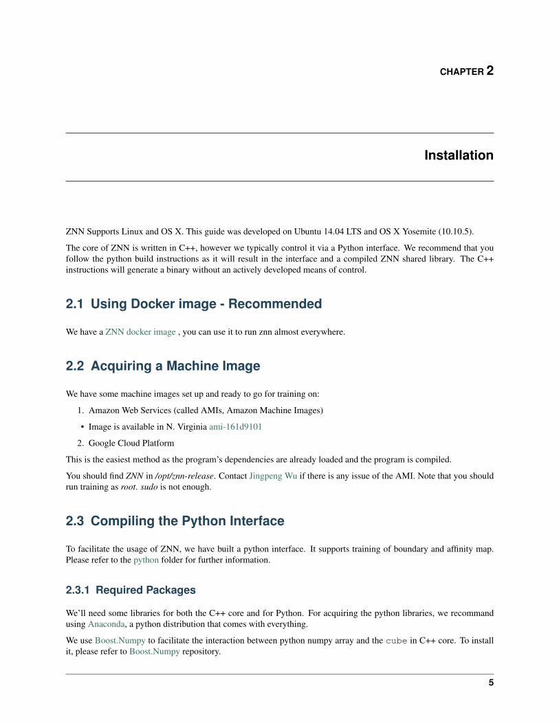
CHAPTER 2

Installation

ZNN Supports Linux and OS X. This guide was developed on Ubuntu 14.04 LTS and OS X Yosemite (10.10.5).

The core of ZNN is written in C++, however we typically control it via a Python interface. We recommend that youfollow the python build instructions as it will result in the interface and a compiled ZNN shared library. The C++instructions will generate a binary without an actively developed means of control.

2.1 Using Docker image - Recommended

We have a ZNN docker image , you can use it to run znn almost everywhere.

2.2 Acquiring a Machine Image

We have some machine images set up and ready to go for training on:

1. Amazon Web Services (called AMIs, Amazon Machine Images)

• Image is available in N. Virginia ami-161d9101

2. Google Cloud Platform

This is the easiest method as the program’s dependencies are already loaded and the program is compiled.

You should find ZNN in /opt/znn-release. Contact Jingpeng Wu if there is any issue of the AMI. Note that you shouldrun training as root. sudo is not enough.

2.3 Compiling the Python Interface

To facilitate the usage of ZNN, we have built a python interface. It supports training of boundary and affinity map.Please refer to the python folder for further information.

2.3.1 Required Packages

We’ll need some libraries for both the C++ core and for Python. For acquiring the python libraries, we recommandusing Anaconda, a python distribution that comes with everything.

We use Boost.Numpy to facilitate the interaction between python numpy array and the cube in C++ core. To installit, please refer to Boost.Numpy repository.

5

ZNN Documentation, Release 0.1.2

2.3.2 Installing Boost.Numpy (OS X)

For convenience, we’ve provided the following incomplete instructions for OS X:

To install Boost.Numpy you’ll need to get boost with Python:

1. Get Homebrew

2. brew install boost --with-python

3. brew install boost-python

4. git clone http://github.com/ndarray/Boost.NumPy

5. ...to be completed. Follow the instructions in the Boost.NumPy repository.

2.3.3 Installing emirt

emirt is a home-made python library specially for neuron reconstruction from EM images.

To install it for ZNN, simply run the following command in the folder of python:

git clone https://github.com/seung-lab/emirt.git

If you find it useful and would like to use it in your other programs, you can also install it in a system path (using yourPYTHONPATH environment variable).

2.3.4 Compile the core of python interface

in the folder of python/core:

make -j number_of_cores

if you use MKL:

make mkl -j number_of_cores

2.4 Compilation of C++ core

The core of ZNN was written with C++ to handle the most computationally expensive forward and backward passes.It is fully functional and can be used to train networks.

2.4.1 Required libraries

Library Ubuntu Package OS X Homebrewfftw libfftw3-dev fftwboost1.55 libboost-all-dev homebrew/versions/boost155

Note that fftw is not required when using intel MKL.

For OS X, you can find the above libraries by consulting the table above and using Homebrew.

6 Chapter 2. Installation

ZNN Documentation, Release 0.1.2

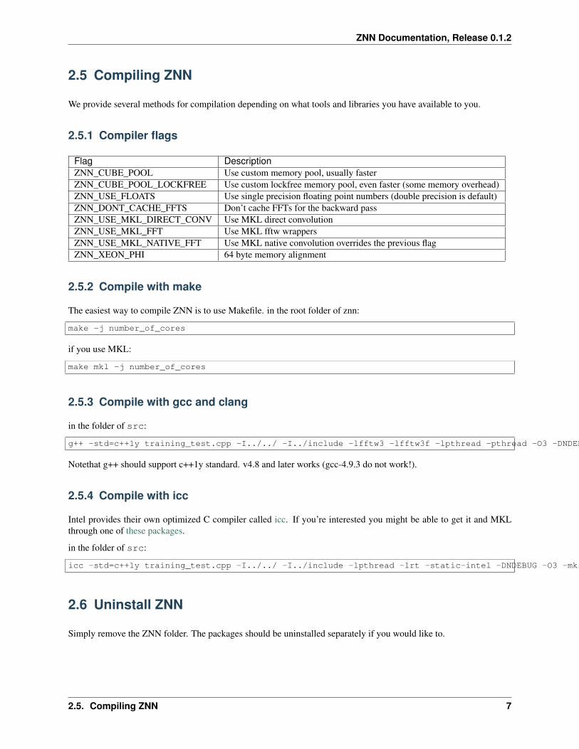
2.5 Compiling ZNN

We provide several methods for compilation depending on what tools and libraries you have available to you.

2.5.1 Compiler flags

Flag DescriptionZNN_CUBE_POOL Use custom memory pool, usually fasterZNN_CUBE_POOL_LOCKFREE Use custom lockfree memory pool, even faster (some memory overhead)ZNN_USE_FLOATS Use single precision floating point numbers (double precision is default)ZNN_DONT_CACHE_FFTS Don’t cache FFTs for the backward passZNN_USE_MKL_DIRECT_CONV Use MKL direct convolutionZNN_USE_MKL_FFT Use MKL fftw wrappersZNN_USE_MKL_NATIVE_FFT Use MKL native convolution overrides the previous flagZNN_XEON_PHI 64 byte memory alignment

2.5.2 Compile with make

The easiest way to compile ZNN is to use Makefile. in the root folder of znn:

make -j number_of_cores

if you use MKL:

make mkl -j number_of_cores

2.5.3 Compile with gcc and clang

in the folder of src:

g++ -std=c++1y training_test.cpp -I../../ -I../include -lfftw3 -lfftw3f -lpthread -pthread -O3 -DNDEBUG -o training_test

Notethat g++ should support c++1y standard. v4.8 and later works (gcc-4.9.3 do not work!).

2.5.4 Compile with icc

Intel provides their own optimized C compiler called icc. If you’re interested you might be able to get it and MKLthrough one of these packages.

in the folder of src:

icc -std=c++1y training_test.cpp -I../../ -I../include -lpthread -lrt -static-intel -DNDEBUG -O3 -mkl=sequential -o training_test

2.6 Uninstall ZNN

Simply remove the ZNN folder. The packages should be uninstalled separately if you would like to.

2.5. Compiling ZNN 7

ZNN Documentation, Release 0.1.2

2.7 Resources

• the travis file shows the step by step installation commands in Ubuntu.

8 Chapter 2. Installation

CHAPTER 3

Tutorial

Now that you have ZNN set up in an environment you want to use, let’s set up an experiment.

Since the python interface is more convenient to use, this tutorial only focuses on it.

3.1 1. Importing Experimental Images

Create a directory called “experiments” in the ZNN root directory. Copy your images to the directory. You’ll want tokeep track of which images are your source images and which are your ground truth. Make sure you create a trainingset and a validation set so that you can ensure your training results are meaningful. If you only have one set of images,split them down the middle.

3.1.1 Image format

The dataset is simply a 3D tif or h5 image stack.

type format bit depthraw image .tif 8label image .tif 32 or RGB

• For training, you should prepare pairs of tif files, one is a stack of raw images, the other is a stack of labeledimages. A label is defined as a unique RGBA color.

• For forward pass, only the raw image stack is needed.

3.1.2 Image configuration

Next create a .spec file that provides the binding between your dataset and ground truth.

The image pairs are defined as a Sample. Start with this example and customize it to suit your needs.

The .spec file format allows you to specify multiple files as inputs (stack images) and outputs (ground truth labels)for a given experiment. A binding of inputs to outputs is called a sample.

The file structure looks like this, where “N” in imageN can be any positive integer. Items contained inside anglebrackets are <option1, option2> etc.

[imageN]fnames = path/of/image1

path/of/image2pp_types = <standard2D, none> # preprocess the image by subtracting mean

9

ZNN Documentation, Release 0.1.2

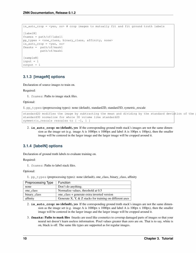
is_auto_crop = <yes, no> # crop images to mutually fit and fit ground truth labels

[labelN]fnames = path/of/label1pp_types = <one_class, binary_class, affinity, none>is_auto_crop = <yes, no>fmasks = path/of/mask1

path/of/mask1

[sampleN]input = 1output = 1

3.1.3 [imageN] options

Declaration of source images to train on.

Required:

1. fnames: Paths to image stack files.

Optional:

1. pp_types (preprocessing types): none (default), standard2D, standard3D, symetric_rescale

standard2D modifies the image by subtracting the mean and dividing by the standard deviation of the pixel values.standard3D normalize for whole 3D volume like standard2Dsymmetric_rescale rescales to [ -1, 1 ]

2. is_auto_crop: no (default), yes If the corresponding ground truth stack’s images are not the same dimen-sion as the image set (e.g. image A is 1000px x 1000px and label A is 100px x 100px), then the smallerimage will be centered in the larger image and the larger image will be cropped around it.

3.1.4 [labelN] options

Declaration of ground truth labels to evaluate training on.

Required:

1. fnames: Paths to label stack files.

Optional:

1. pp_types (preprocessing types): none (default), one_class, binary_class, affinity

Preprocessing Type Functionnone Don’t do anything.one_class Normalize values, threshold at 0.5binary_class one_class + generate extra inverted versionaffinity Generate X, Y, & Z stacks for training on different axes

2. is_auto_crop: no (default), yes If the corresponding ground truth stack’s images are not the same dimen-sion as the image set (e.g. image A is 1000px x 1000px and label A is 100px x 100px), then the smallerimage will be centered in the larger image and the larger image will be cropped around it.

3. fmasks: Paths to mask files fmasks are used like cosmetics to coverup damaged parts of images so that yourneural net doesn’t learn useless information. Pixel values greater than zero are on. That is to say, white ison, black is off. The same file types are supported as for regular images.

10 Chapter 3. Tutorial

ZNN Documentation, Release 0.1.2

3.1.5 [sampleN] options

Declaration of binding between images and labels. You’ll use the sample number in your training configuration todecide which image sets to train on.

Required:

1. input: (int > 0) should correspond to the N in an [imageN]. e.g. input: 1

2. output: (int > 0) should correspond to the N in a [labelN]. e.g. output: 1

3.2 2. Network Architecture Configuration

We have a custom file format .znn for specifying the layout of your neural network. It works based on a few simpleconcepts.

1. Each of the input nodes of the network represent an image stack.

2. The network consists of layers whose size can be individually specified.

3. The edge betwen the layers specify not only the data transfer from one layer to another (e.g. one to one, or fullyconnected), they also prescribe a transformation, e.g. a filter or weight, to be applied.

4. After all the weights or filters have been applied, the inputs are summed and a pixel-wise transfer function (e.g.a sigmoid or ReLU) is applied.

5. The type of the edges determines if the layers its connecting is a one-to-one mapping or is fully connected. Forexample, a convolution type will result in fully connected layers.

6. The output layer represents whatever you’re training the network to do. One common output is the predictedlabels for an image stack as a single node.

You can find example network N4 here.

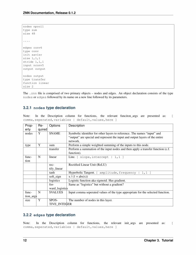
Here’s an example excepted from the N4 network:

nodes inputtype inputsize 1

edges conv1type convinit xaviersize 1,4,4stride 1,1,1input inputoutput nconv1

nodes nconv1type transferfunction rectify_linearsize 48

edges pool1type max_filtersize 1,2,2stride 1,2,2input nconv1output npool1

3.2. 2. Network Architecture Configuration 11

ZNN Documentation, Release 0.1.2

nodes npool1type sumsize 48

....

edges conv6type convinit xaviersize 1,1,1stride 1,1,1input nconv5output output

nodes outputtype transferfunction linearsize 2

The .znn file is comprised of two primary objects – nodes and edges. An object declaration consists of the typenodes or edges followed by its name on a new line followed by its parameters.

3.2.1 nodes type declaration

Note: In the Description column for functions, the relevant funciton_args are presented as: [comma,seperated,variables | default,values,here ]

Prop-erty

Re-quired

Options Description

nodes Y $NAME Symbolic identifier for other layers to reference. The names “input” and“output” are special and represent the input and output layers of the entirenetwork.

type Y sum Perform a simple weighted summing of the inputs to this node.transfer Perform a summation of the input nodes and then apply a transfer function (c.f.

function).func-tion

N linear Line. [ slope,intercept | 1,1 ]

rec-tify_linear

Rectified Linear Unit (ReLU)

tanh Hyperbolic Tangent. [ amplitude,frequency | 1,1 ]soft_sign x / (1 + abs(x))logistics Logistic function aka sigmoid. Has gradient.for-ward_logistics

Same as “logistics” but without a gradient?

func-tion_args

N $VALUES Input comma seperated values of the type appropriate for the selected function.

size Y $POS-TIVE_INTEGER

The number of nodes in this layer.

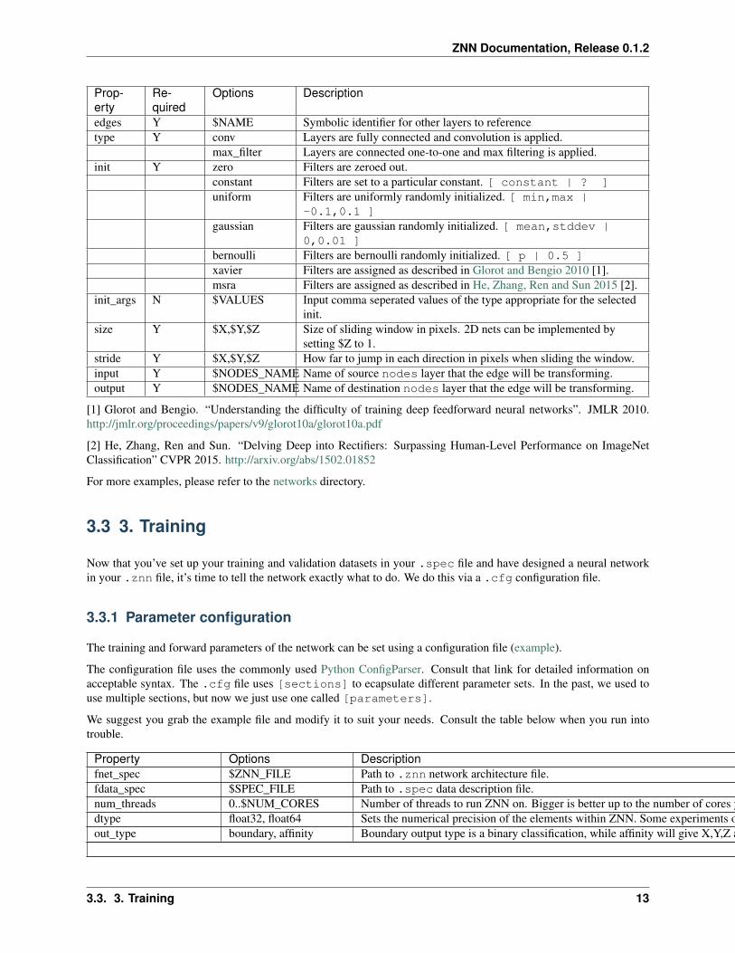
3.2.2 edges type declaration

Note: In the Description column for functions, the relevant init_args are presented as: [comma,seperated,variables | default,values,here ]

12 Chapter 3. Tutorial

ZNN Documentation, Release 0.1.2

Prop-erty

Re-quired

Options Description

edges Y $NAME Symbolic identifier for other layers to referencetype Y conv Layers are fully connected and convolution is applied.

max_filter Layers are connected one-to-one and max filtering is applied.init Y zero Filters are zeroed out.

constant Filters are set to a particular constant. [ constant | ? ]uniform Filters are uniformly randomly initialized. [ min,max |

-0.1,0.1 ]gaussian Filters are gaussian randomly initialized. [ mean,stddev |

0,0.01 ]bernoulli Filters are bernoulli randomly initialized. [ p | 0.5 ]xavier Filters are assigned as described in Glorot and Bengio 2010 [1].msra Filters are assigned as described in He, Zhang, Ren and Sun 2015 [2].

init_args N $VALUES Input comma seperated values of the type appropriate for the selectedinit.

size Y $X,$Y,$Z Size of sliding window in pixels. 2D nets can be implemented bysetting $Z to 1.

stride Y $X,$Y,$Z How far to jump in each direction in pixels when sliding the window.input Y $NODES_NAME Name of source nodes layer that the edge will be transforming.output Y $NODES_NAME Name of destination nodes layer that the edge will be transforming.

[1] Glorot and Bengio. “Understanding the difficulty of training deep feedforward neural networks”. JMLR 2010.http://jmlr.org/proceedings/papers/v9/glorot10a/glorot10a.pdf

[2] He, Zhang, Ren and Sun. “Delving Deep into Rectifiers: Surpassing Human-Level Performance on ImageNetClassification” CVPR 2015. http://arxiv.org/abs/1502.01852

For more examples, please refer to the networks directory.

3.3 3. Training

Now that you’ve set up your training and validation datasets in your .spec file and have designed a neural networkin your .znn file, it’s time to tell the network exactly what to do. We do this via a .cfg configuration file.

3.3.1 Parameter configuration

The training and forward parameters of the network can be set using a configuration file (example).

The configuration file uses the commonly used Python ConfigParser. Consult that link for detailed information onacceptable syntax. The .cfg file uses [sections] to ecapsulate different parameter sets. In the past, we used touse multiple sections, but now we just use one called [parameters].

We suggest you grab the example file and modify it to suit your needs. Consult the table below when you run intotrouble.

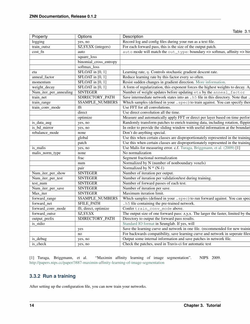
Property Options Descriptionfnet_spec $ZNN_FILE Path to .znn network architecture file.fdata_spec $SPEC_FILE Path to .spec data description file.num_threads 0..$NUM_CORES Number of threads to run ZNN on. Bigger is better up to the number of cores you have. 0 will automatically select the maximum.dtype float32, float64 Sets the numerical precision of the elements within ZNN. Some experiments on 64 bit machines show a 2x speedup with float32. If you change this, you’ll need to recompile after setting or unsetting ZNN_USE_FLOATS in the Makefile.out_type boundary, affinity Boundary output type is a binary classification, while affinity will give X,Y,Z affinities between neighboring voxels.

Continued on next page

3.3. 3. Training 13

ZNN Documentation, Release 0.1.2

Table 3.1 – continued from previous pageProperty Options Descriptionlogging yes, no Record log and config files during your run as a text file.train_outsz $Z,$Y,$X (integers) For each forward pass, this is the size of the output patch.cost_fn auto auto mode will match the out_type: boundary => softmax, affinity => binomial

square_lossbinomial_cross_entropysoftmax_loss

eta $FLOAT in [0, 1] Learning rate, 𝜂. Controls stochastic gradient descent rate.anneal_factor $FLOAT in [0, 1] Reduce learning rate by this factor every so often.momentum $FLOAT in [0, 1] Resist sudden changes in gradient direction. More information.weight_decay $FLOAT in [0, 1] A form of regularization, this exponent forces the highest weights to decay. Applied after every iteration.Num_iter_per_annealing $INTEGER Number of weight updates before updating eta by the anneal_factortrain_net $DIRECTORY_PATH Save intermediate network states into an .h5 file in this directory. Note that .h5 can store more than just image data. If you don’t provide a seed (see “Resume a Training” below), this will automatically load.train_range $SAMPLE_NUMBERS Which samples (defined in your .spec) to train against. You can specify them like 1-3,6 if you wanted to train 1,2,3, and 6.train_conv_mode fft Use FFT for all convolutions.

direct Use direct convolution all the time.optimize Measure and automatically apply FFT or direct per layer based on time performance. Note, this can take several minutes.

is_data_aug yes, no Randomly transform patches to enrich training data, including rotation, flipping.is_bd_mirror yes, no In order to provide the sliding window with useful information at the boundaries, mirror the image near the boundaries.rebalance_mode none Don’t do anything special.

global Use this when certain classes are disproportionately represented in the training data. This will rebalance the learning process by the global fraction of voxels that each class comprises.patch Use this when certain classes are disproportionately represented in the training data. This will rebalance the learning process by the patch fraction of voxels that each class comprises.

is_malis yes, no Use Malis for measuring error. c.f. Turaga, Briggmann, et al. (2009) [1]malis_norm_type none No normalization

frac Segment fractional normalizationnum Normalized by N (number of nonboundary voxels)pair Normalized by N * (N-1)

Num_iter_per_show $INTEGER Number of iteration per output.Num_iter_per_test $INTEGER Number of iteration per validation/test during training.test_num $INTEGER Number of forward passes of each test.Num_iter_per_save $INTEGER Number of iteration per save.Max_iter $INTEGER Maximum iteration limit.forward_range $SAMPLE_NUMBERS Which samples (defined in your .spec) to run forward against. You can specify them like 1-3,6 if you wanted to train 1,2,3, and 6.forward_net $FILE_PATH .h5 file containing the pre-trained network.forward_conv_mode fft, direct, optimize Confer train_conv_mode above.forward_outsz $Z,$Y,$X The output size of one forward pass: z,y,x. The larger the faster, limited by the memory capacity.output_prefix $DIRECTORY_PATH Directory to output the forward pass results.is_stdio Standard IO format in Seunglab. If yes, will

yes Save the learning curve and network in one file. (recommended for new training)no For backwards compatibility, save learning curve and network in seperate files.

is_debug yes, no Output some internal information and save patches in network file.is_check yes, no Check the patches, used in Travis-ci for automatic test

[1] Turaga, Briggmann, et al. “Maximin affinity learning of image segmentation”. NIPS 2009.http://papers.nips.cc/paper/3887-maximin-affinity-learning-of-image-segmentation

3.3.2 Run a training

After setting up the configuration file, you can now train your networks.

14 Chapter 3. Tutorial

ZNN Documentation, Release 0.1.2

Make sure you run the following command from within the znn-release/python directory. This is a limitation that canbe fixed in future releases.

python train.py -c path/of/config.cfg

3.3.3 Resume a training

Since the network is periodically saved, we can resume training whenever we want to. By default, ZNN will auto-matically resume the latest training net (net_current.h5) in a folder, which was specified by the train_netparameter in the configuration file.

To resume training a specific network, we can use the seeding function:

python train.py -c path/of/config.cfg -s path/of/seed.h5

3.3.4 Transfer learning

Sometimes, we would like to utilize a trained network. If the network architectures of trained and initialized networkare the same, we call it Loading. Otherwise, we call it Seeding, in which case the trained net is used as a seed toinitialize part of the new network. Our implementation merges Loading and Seeding. Just use the synonymous-s or --seed command line flags.

python train.py -c path/of/config.cfg -s path/of/seed.h5

3.4 Forward Pass

run the following command:

python forward.py -c path/of/config.cfg

if you are running forward pass intensively for a large image stack, it is recommanded to recompile python coreusing DZNN_DONT_CACHE_FFTS. Without caching FFTS, you can use a large output size, which reuse a lot ofcomputation and speed up your forward pass.

NOTE: If your forward pass aborts without writing anything, try reducing the output size, as you may have run out ofmemory.

3.4. Forward Pass 15

ZNN Documentation, Release 0.1.2

16 Chapter 3. Tutorial

CHAPTER 4

Indices and tables

• genindex

• modindex

• search

17