Zoltán Monostori

Essays on government debt financing

costs

Institute of Finance, Accounting and Law

Department of Finance

Supervisor:

Edina Berlinger Ph.D.

© Zoltán Monostori

CORVINUS UNIVERSITY OF BUDAPEST

Management and Business Administration

Doctoral School

Zoltán Monostori

Essays on government debt financing costs

Ph.D. Dissertation

Budapest, 2014

5

Table of contents

I. Foreword .............................................................................................................................. 9

I.1. Background, actuality .................................................................................................... 9

I.2. Methodology .................................................................................................................. 10

I.3. Results ............................................................................................................................ 13

I.4. Practice .......................................................................................................................... 14

I.5. Own publications .......................................................................................................... 15

I.6. Structure ........................................................................................................................ 16

II. Discriminatory versus uniform-price auctions ......................................................... 18

II.1. Introduction .................................................................................................................. 18

II.2. Theoretical results ...................................................................................................... 22

II.2.1. Theorems for single-unit auctions .................................................................. 22

II.2.2. Misconceptions in connection with multi-unit auctions ............................ 25

II.2.3. Bid curves submitted in multi-unit auctions ................................................ 26

II.2.4. Winner’s curse ..................................................................................................... 27

II.2.5. Risk aversion ........................................................................................................ 28

II.2.6. Fog of war ............................................................................................................. 29

II.2.7. Secondary market, forward market, collusion ............................................ 30

II.2.8. Summary of theoretical results ....................................................................... 33

II.3. Laboratory experiments ............................................................................................. 34

II.4. Non-laboratory empirical evidence.......................................................................... 35

II.4.1. Empirical evidence of uniform-price auctions ............................................ 36

II.4.2. Empirical evidence of discriminatory-price auctions ................................ 37

II.4.3. Empirical comparison of uniform-price and discriminatory-price

auctions .............................................................................................................................. 42

II.5. International practice................................................................................................. 49

II.6. Summary and conclusion ............................................................................................ 50

III. Country-Specific Determinants of Sovereign CDS spreads: The Role of

Fundamentals in Eastern Europe ........................................................................................... 56

III.1. Introduction ................................................................................................................. 57

III.2. Literature review ....................................................................................................... 63

III.2.1. Sovereign spreads and default risk ............................................................... 63

III.2.2. Non-credit risk factors ...................................................................................... 69

III.3. Data and Methodology ............................................................................................... 71

6

III.3.1. Data ....................................................................................................................... 71

III.3.2. Methodology ........................................................................................................ 79

III.4. Results .......................................................................................................................... 85

III.4.1. General results ................................................................................................... 85

III.4.2. Have the aspects of differentiation between countries changed

through time? ................................................................................................................... 91

III.4.3. Robustness checks ............................................................................................. 93

III.5. Conclusions .................................................................................................................. 95

IV. Application to the Hungarian CDS spread ................................................................ 97

IV.1. Introduction, stylized facts ...................................................................................... 97

IV.2. Model explanations for the deterioration ........................................................... 100

IV.3. Explanations for the residuals of the model ...................................................... 105

IV.4. Conclusion .................................................................................................................. 108

V. Summary ...................................................................................................................... 109

VI. Appendices .................................................................................................................. 116

VI.1. Appendix 1: The Revenue Equivalence Theory ................................................... 116

VI.2. Appendix 2: The Database ...................................................................................... 117

VI.3. Appendix 3: Coefficient estimates of rolling window regressions ................. 119

VI.4. Appendix 4: Robustness checks .............................................................................. 121

VI.5. Appendix 5: Panel Cointegration Test ................................................................. 123

VI.6. Appendix 6: Application to the Polish CDS spread ............................................ 124

VI.7. Appendix 7: Application to the Russian CDS spread .......................................... 129

VI.8. Appendix 8: Application to the Turkish CDS spread .......................................... 135

VI.9. Appendix 9: Graphs about relative fundamentals ............................................. 141

VII. References ................................................................................................................... 146

VIII. Publications of the author in this topic ................................................................. 166

VIII.1. Publications in Hungarian ..................................................................................... 166

VIII.2. Publications in English .......................................................................................... 167

7

List of Tables

List of Figures

Table 1: Theoretical studies comparing uniform-price and discriminatory-price auctions 33

Table 2: Studies comparing uniform-price and discriminatory-price auctions 47

Table 3: Treasuries using the various auction methods 49

Table 4: Long-run regression results 86

Table 5: Short-run regression results 89

Table 6: Data 117

Table 7: Principal components 118

Table 8: Factors 118

Table 9: Robustness checks: estimation on quarterly data and cross-section subsamples 121

Table 10: Robustness checks: estimations including and excluding Hungary from the sample 122

Table 11: Panel Cointegration Test 123

Figure 1: Expected revenue from uniform-price and discriminatory-price auctions 20

Figure 2: Relative position of bid functions 24

Figure 3: Explanatory power differences of restricted and unrestricted long-run regressions 92

Figure 4: Hungarian 5-year CDS spreads and the Eastern European average 98

Figure 5: Hungarian indicators compared to regional averages 99

Figure 6: Relative CDS spreads 100

Figure 7: Contributions to the model-based value of the relative CDS spread 102

Figure 8: Fundamental and wake-up call effects in changes of Hungarian spreads 104

Figure 9: The Hungarian relative CDS spread and its unexplained component 105

Figure 10: Coefficient estimates of the long-run panel regressions on two-year rolling windows 119

Figure 11: Coefficient estimates of the long-run panel regressions on one-year rolling windows 120

Figure 12: Polish 5-year CDS spreads and the Eastern European average (July 2008 – March 2012) 124

Figure 13: Poland: Contributions to the model-based value of the relative CDS spread 125

Figure 14: Polish indicators compared to regional averages 126

Figure 15: The Polish relative CDS spread and its unexplained component 127

Figure 16: Fundamental and wake-up call effects in changes of Polish spreads 128

Figure 17: Russian 5-year CDS spreads and the Eastern European average (July 2008 – March 2012) 129

Figure 18: Russia: Contributions to the model-based value of the relative CDS spread 131

Figure 19: Russian indicators compared to regional averages 132

Figure 20: The Russian relative CDS spread and its unexplained component 133

Figure 21: Fundamental and wake-up call effects in changes of Russian spreads 134

Figure 22: Turkish 5-year CDS spreads and the Eastern European average (July 2008 – March 2012) 135

Figure 23: Turkey: Contributions to the model-based value of the relative CDS spread 137

Figure 24: Turkish indicators compared to regional averages 138

Figure 25: The Turkish relative CDS spread and its unexplained component 139

Figure 26: Fundamental and wake-up call effects in changes of Turkish spreads 140

Figure 27: Log CDS spread compared to regional averages 141

Figure 28: PC_GROWTH compared to regional averages 142

Figure 29: F_BANK compared to regional averages 142

Figure 30: F_EXTERN compared to regional averages 143

Figure 31: F_GDEBT compared to regional averages 143

Figure 32: PC_INST compared to regional averages 144

Figure 33: FISCBAL compared to regional averages 144

Figure 34: RATINGS compared to regional averages 145

Figure 35: RATING_RESIDS compared to regional averages 145

8

I am most grateful to Edina Berlinger, my Ph. D. thesis supervisor and my

colleagues Judit Antal, Csaba Csávás, Áron Gereben, Viola Monostoriné

Grolmusz, Zsolt Kuti and Zoltán Reppa for their suggestions and assistance. I

am indebted to Gyula Magyarkuti, who taught me mathematical auction

theory in a Ph. D. course. I am grateful to Péter Bárczy and Alexandra

Szatmári for their valuable comments. I am indebted to Zalán Kocsis, who was

an ideal co-author of a paper also used in some parts of this dissertation. I am

grateful to Zsolt Kuti, who had also some contribution in these parts.

I would like to thank my wife, Viola Monostoriné Grolmusz, not only for her

professional assistance, but also for her love, kindness and support she has

shown during the past two years it has taken me to finalize this thesis.

Furthermore I would also like to thank my parents for their endless love and

support

9

I. FOREWORD

I.1. Background, actuality

In the recent years, more and more countries had to face the problem that

their government debt / gross domestic product quotients dynamics were not

sustainable. The most important factors in this process were smaller growth,

bad structural balance of the budget, and high financing costs of the

government debt, which is related to the increasing sovereign yields. These

three factors are closely related, but we can highlight that on the one hand,

raising the growth rate and balancing the budget could be done by using

either different (for example positive fiscal stimulus vs. fiscal tightening) or

very unpopular measures (like making more flexible working laws, or raising

the retirement age). On the other hand, it might be possible to reach success

by decreasing the sovereign yields.

The primary market of government bills and bonds is one of the most

important fields where financing costs of government debt are evolving. The

primary market affects financing costs through the selling price of

government bills and bonds. These securities are in many cases – as for

example the domestic papers in Hungary - sold through auctions. Nowadays,

two auction techniques (discriminatory and uniform-price auctions) are most

commonly used for the sale of securities, specifically government bills and

bonds. Since the selling price of the papers is influenced by the technique of

the auction, a comparison of the discriminatory and uniform-price auctions

would be helpful to determine which of the two most commonly used auction

formats is the optimal allocation mechanism under given conditions.

The financing costs of the government debt are also strongly related to the

country’s credit risk, measured mostly through sovereign CDS spreads. This

has two reasons. First, the foreign currency denominated bond yields can be

decomposed to a risk-free yield (like the sovereign German Euro-yield or the

USA Dollar-yield) and the rest of the bond yield, which is called bond spread.

The bond spread is generally near to the CDS spread, and CDS spreads tend to

10

lead bond spreads (Alper et al. [2012]; Varga [2009]). Second, in the case of

domestic bonds, the credit risk of the country also has a significant effect on

yields on the longer terms. The credit risk premium of the local currency

denominated bonds might be somewhat different from CDS spreads, but CDS

spreads have a significant co-movement with long term domestic yields

(Monostori [2012b], Monostori [2013e]). While sovereign credit risk and CDS

spreads are very actual topics also in academia, our research question has

some traditional background. Part III’s objective is to empirically assess the

role of country-specific fundamental determinants in shaping Eastern

European relative CDS spreads.

Part IV is an application of the model to the Hungarian CDS spreads. In this

case study we identify the country-specific determinants of the last years’

processes of Hungarian CDS spreads.

I.2. Methodology

The expected revenue of uniform-price and discriminatory auctions cannot be

ranked definitively based on analytical studies; therefore it may be

appropriate to approach this issue on an empirical basis. The empirical

evidence of real-world auctions provide a robust answer to the question of

expected revenue; the uniform-price format coming out as more beneficial

for the Treasury. Experiments fall into two categories: in the first case,

comparison is enabled by the fact that the auction format of identical goods

was changed from a given time, while in the other case, there were other

treasuries to auction different products in a close-to-identical time interval

with different methods. However, all experiments have been plagued by the

identification problem, that is, the change caused by the auction method is

difficult to tell apart from the effects of other circumstances. It would be a

real scientific breakthrough, though, to set up a real-life experiment in which

the same product would be sold simultaneously in both uniform-price and

discriminatory auctions. Even though fewer conclusions could be drawn than

in the previously proposed arrangement (due to the repetition of auctions), it

would be instructive to see an experiment where primary market actors have

11

to submit bids for both auction formats, then the real format would be

decided by drawing lots. We should note, however, that the experiment may

increase the ‘fog of war’, i.e. the strategy space may become even more

complicated and the number of possible equilibria may increase to extreme

heights. Such an experiment could be a very important step in future work;

however, it has to be supported by a bond issuer.

Hence, in Part II our methodology is a comparative analysis through the

relevant literature about discriminatory and uniform price auctions. The same

methodology is used by such important papers in this topic as Das & Sundaram

[1997]; Binmore & Swierzbinski [2000], or in Hungary (Szatmári [1996b]), and

the most recent Hungarian study of this subject, (Kondrát [1996]). The latter

Hungarian papers focused primarily on models based on the unit demand

assumption; whereas researchers have demonstrated that these findings are

often not applicable to all of the multi-unit auctions, so a new review might

be reasonable.

In Part III we take the traditional and simple methodological approach of

Edwards ([1983]; [1985]) and a wealth of publications since to date. We

adhere to the literature in assuming that most of the time series variation in

CDS spreads are a result of common shocks to the pricing of risk and we

concentrate the analysis on the other, cross-sectional aspect of CDS spreads

by assessing which fundamental factors have been empirically important in

explaining the relative riskiness of countries as proxied by the relative

magnitude of these indicators. In terms of estimation methodology we use a

time fixed effects panel regression on both the levels and changes of spreads

and fundamental variables. We link the short-run dynamics with the

relationship between variable levels through an error-correction term.

We lay emphasis on using a dataset that treats some empirical issues that, in

previous studies, have often been disregarded. First, we use projections of

future variables instead of actual data where possible. CDS spreads (and bond

spreads) derive from expected future cash flows during the tenor of the

instrument. Therefore it is arguably the expectations of the variables

12

influencing credit spreads (growth, budget balance, etc.) and not the actual

data available at the time that matters. Using actual data instead of

expectations introduces a source of error, and it will contaminate inference

on how the variable affects spreads. This error will be larger for variables

whose expectations are in general more volatile. Also, a mistake can be made

in assessing the explanatory power of macroeconomic variables when

comparing their actual data with financial time series. Though

macroeconomic variables change (or are observed) infrequently, while

financial indicators fluctuate on high frequency, it may be the case that the

expectation of macroeconomic variables is just as volatile as the financial

time series and that this explains more of the latter’s variation than actual

data. Second, we aim to reduce the adverse effects of variable omissions by

including a larger and conceptually wider set of fundamental variables than

usual in similar studies. Besides the standard macroeconomic variables, we

incorporate data on the banking sector and use a set of political and

institutional variables as well.

Principal components and factors are extracted from conceptually similar

variables’ groups and these are then used in CDS spreads’ regressions to

overcome problems of multicollinearity and the curse of dimensionality. To

further limit adverse effects of variable omission, we attempt to make use of

the extra information contained in credit ratings compared to that in our

fundamental variable set.

Although we do not explicitly incorporate cross-section and time period

heterogeneity of fundamental variables’ effects in our baseline model, we do

check the robustness of our general results on subsamples. Also, regressions

are re-estimated on shorter time windows to gain an intuition on how

coefficients have evolved through time.

In Part IV we apply the model from Part III to Hungarian data. We use simple

descriptive statistics to analyze the latest developments. To quantify the two

distinct effects on the relative Hungarian CDS spread, i.e. the worsening of

fundamentals and the shift in investor preferences (the wake-up call effect),

13

we use the Oaxaca-Blinder decomposition (Blinder [1973]; Oaxaca [1973]). In

particular we decompose the difference between the model-implied value for

March 2012 due to the 2010-2012 period estimates and the model-implied

value for January 2010 due to the full sample estimates.

I.3. Results

In Part II, theoretical models arrive at different rankings for expected

revenue; however, they do reveal the relationship between the bids

submitted and the auction technique. These results are confirmed both by

‘laboratory’ experiments and the empirical evidence of real-world auctions.

The latter may also provide a robust answer to the question of expected

revenue; the uniform-price format coming out as more beneficial for the

Treasury. Still, at present the global majority of issuers of government bonds

use the discriminatory-price format and central bank instruments also tend to

be sold in this format. This is because issuers may have considerations other

than expected revenue.

The main advantages of the uniform price auction method might be: higher

expected revenue, low markup between the market price and the auction

price (in the long-term average), and increased participation in the auctions.

The discriminatory auctions are able to reduce volatility, reveal the true

valuations better, and hinder price-manipulations.

In the case of the auction of Hungarian government bonds, maximizing the

expected revenue of the issuer may be important. Changing the auction

format (or conducting an experiment into such a change) would be relevant if

volatility remained persistently low with consistently high bid-to-cover ratios.

In Part III we study the relationship between relative sovereign CDS spreads

and a wide array of relative country-specific fundamentals on Eastern

European data between July 2008 and March 2012. We find a significant effect

of growth expectations, banking system stability, government debt and the

institutional-political background in the long-term relationship of relative CDS

14

spreads. Changes of these fundamental variables mainly affect CDS spreads

gradually, through an error-correction mechanism. Contrary to other studies

we do not find higher fiscal deficit being associated with higher CDS spreads,

which may be a result of reverse causality between credit risk and fiscal

balance. Our results suggest that some of the fundamental variable’s impacts

are time-varying and imply relevance of the wake-up call hypothesis.

In Part IV the model discussed in the previous part attributes the Hungarian

CDS spread’s relative increase to both a worsening of fundamentals (growth

prospects and banking stability) and to a changing in investor preferences:

government debt, one of the country’s key weaknesses, has become more

important in relative sovereign risk assessment.

I.4. Practice

While in Hungary, the Government Debt Management Agency (ÁKK) still

uses the discriminatory format, a verification of the auction method might be

particularly topical as, following similar steps by other treasuries, the public

debt management agency of a country in the Central-Eastern-European

region, Poland, switched to the uniform-price system in January 2012. Since a

decrease of 1 basis point in the selling yields could spare the budget in the

long term yearly more than one billion Hungarian Forints 1 , this topic is

important. The analysis may also be useful in reconsidering the form of

auction for the central bank instruments introduced during the crisis and for

the design of the format for the sale of any new instruments to be launched in

the future.

Sovereign CDS spreads have received increasing attention in the past

several years. The financial crisis of 2007-2008 and the ensuing sovereign

crisis of the Eurozone periphery have increased activity in sovereign CDS

1 The outstanding amount of Forint denominated government bills and bonds was 12 977

billion Forints in June 2013. Source: MNB.

http://www.mnb.hu/Root/Dokumentumtar/MNB/Statisztika/mnbhu_statisztikai_idosorok/a-

rezidens-kibocsatasu-ertekpapirok-adatai-kibocsatoi-es-tulajdonosi-

bontasban/Havi_adatok_hu.xls

15

markets and broadened the market’s scope from emerging markets with large

bond portfolios in the pre-crisis era to the smaller emerging markets and

eventually to developed economy sovereigns. Market participants used the

instrument to either take a speculative position on the credit risk outlook of

sovereigns, or to hedge credit risk exposure through bonds; whereas analysts,

central banks and the financial media observed the market to gauge the

perceived credit risk of sovereigns.

In economic policy debates, it is an often argued point whether the change of

sovereign CDS spreads was based on fundamentals in a volatile environment2.

Our model is able to estimate a relative CDS spread based on fundamentals,

so the spread between the model-based and observed CDS spreads might have

important information content in these debates.

In our model some coefficients seem to be sensitive to the selection of the

country sample. Time-variation of parameters is supported by simple rolling

regressions, pointing to an increase of government debt, banking stability and

external balance in the assessment of relative riskiness of countries, which

might be important in setting economic policy goals.

I.5. Own publications

Part II was discussed at the November 15, 2012 meeting of the Monetary

Forum, it has been presented at several conferences and it is published in

Hungarian in the Közgazdasági Szemle (Monostori [2013c]) and in English in

MNB Occasional Papers (Monostori [2014]).

The author has also other publications concerning government debt

financing costs. Monostori [2012b] at Hitelintézeti Szemle is a paper about risk

premia of government bond yields. Another paper at Society and Economy

(Monostori [2013e]) is about sovereign bond market liquidity developments on

the Hungarian market. While the article in MNB Bulletin (Erhart et al. [2013])

2 Policy makers (also Monetary Council members) often argue that observed CDS spreads will

tend to fundamental-based eqilibria in the long term.

16

is not exactly about government debt financing costs, that topic (central

banks’ balance sheet strategies) is nowadays also related to the main topic of

the dissertation.

Part III and Part IV are published only at conferences this moment (Kocsis –

Monostori, [2013a]; Kocsis – Monostori, [2013b]); however another output of

the same research will be submitted in the upcoming weeks to Economics of

Transition. These parts are results of a common research with Zalán Kocsis

(and Zsolt Kuti also had some significant contribution).

Also some further conference publications are worth mentioning.

(Monostori [2013a]; [2013b]; [2013d]; [2012a]; [2012c]; [2012d]; [2011a];

[2011b]; [2010]).

I.6. Structure

The structure of the dissertation is as follows.

The main question of the following part (Part II) is: which one of the most

commonly used (discriminatory- and uniform price) auction formats has the

more beneficial effect on government debt financing costs. This part starts

with an introduction, which is followed by theoretical models. Next, empirical

(both laboratory and non-laboratory) evidences are presented which is

followed by the description of the international practice. The part is finished

by summary and conclusions.

In Part III, the main question is: which fundamentals are the most

important country-specific determinants of sovereign CDS spreads in Eastern

Europe. After the introduction and literature review, data and methodology

are described. Next, we present the general results, the varying of the most

important factors in time and robustness checks. Finally, we conclude.

Part IV investigates the Hungarian sovereign CDS spread’s developments

through our model in the last few years. After introducing and presenting the

stylized facts, model explanations for the deterioration are shown. Then we

give explanations for the residuals of the model, and finally we conclude this

part.

17

Part V gives a summary about the most important results of the

dissertation.

18

II. DISCRIMINATORY VERSUS UNIFORM-PRICE AUCTIONS

The financing costs of government debt are strongly affected by the selling

price of government bills and bonds. These securities are in many cases –

as for example the domestic papers in Hungary - sold through auctions.

The selling price of a paper is influenced by the technique of the auction.

The purpose of this part is to compare the two auction techniques

(discriminatory and uniform-price auctions) most commonly used for the

sale of securities. Literature tends to analyze methods from the aspect of

the expected revenue from the auction. Theoretical models arrive at

different rankings for expected revenue; however, they do reveal the

relationship between the bids submitted and the auction technique. These

results are confirmed both by ‘laboratory’ experiments and the empirical

evidence of real-world auctions. The latter may also provide a robust

answer to the question of expected revenue; the uniform-price format

coming out as the more beneficial for the Treasury. Still, at present the

global majority of issuers of government bonds use the discriminatory-

price format and central bank instruments also tend to be sold in this

format. This is because issuers may have considerations other than

expected revenue.

II.1. Introduction

The purpose of the paper is to give a comprehensive overview of literature

to discuss if the uniform-price or the discriminatory auction format is the

better allocation mechanism under given conditions. This review is

particularly topical as, following similar steps by other treasuries, the public

debt management agency of a country in the Central-Eastern-European

region, Poland, switched to the uniform-price system in January 2012. The

part concludes with a policy recommendation on whether it is expedient for

the Government Debt Management Agency (ÁKK) to continue with

19

discriminatory auctions given the current state of the government bond

market and the primary dealer system. The analysis may also be useful in

reconsidering the form of auction for the central bank instruments introduced

during the crisis and for the design of the format for the sale of any new

instruments to be launched in the future.

In most countries around the world, the issued government securities are

allocated through auctions, even though subscription-based syndicated issues

did survive for quite some time in England and Japan, for instance. The

across-the-board popularity of auctions is attributable to the fact that they

assure the scheduled, regular, safe financing of public debt at a low cost and

at a close-to-market price.

The two auction methods most frequently used in this area are

discriminatory and uniform-price auctions. In both cases, the issuer ranks the

bids received for the homogeneous products by price, in a descending order.

Then it accepts bids in that order, going from highest to lowest, until the

intended volume is taken up or all the bids are accepted. (That is, the highest

bids for the given volume are accepted.) If at the lowest accepted price the

quantity demanded is higher than the residual quantity of issuable products,

then the residual quantity is distributed among bidders according to the

proportions of their submitted bids at this price. The two formats differ in

that while in discriminatory-price auctions financial settlement occurs at the

different prices indicated in the bids, in uniform-price auctions the winning

bidders all end up paying the price indicated in the highest rejected bid.

These two auction mechanisms have the following impact on the expected

revenue of the auctioneer: while participants may be assumed to submit

higher bids for uniform-price auctions3, the average price of the accepted bids

at discriminatory auctions may be increased by price discrimination (Figure

1). Thus a switch to the uniform-price auction method may be successful in

terms of expected revenue if the area between points BCD is larger than the

opportunity cost DEF, therefore the revenue from the uniform-price auction

3 Almost every accepted bidder pays less than their bid.

20

(ACFG rectangle) is greater than the revenue from the discriminatory auction

(ABEG trapezoid).

Figure 1. Expected revenue from uniform-price and discriminatory-price

auctions

Source: own figure, based on (Kondrát [1996])

Even though literature tends to examine auctions mostly from the aspect of

the expected revenue of the auctioneer, we should note that the Treasury

may have other considerations as well4. These may include efficiency (i.e.

4 As a very simple approximation for the effect on the expected revenue, we can state the

following: the amount of the Hungarian Forint denominated government debt is

approximately 13 000 billion HUFs (FX denominated debt is not allocated through auctions

nowadays in Hungary: FX-bonds are allocated subscription-based at road shows, loans are

naturally not auctioned). If another auction method could reduce the yields of the newly

issued government debt, every basis point gained in the yearly yields could save around 0.01

percent for the state in the long term (when every previously issued paper ran out), that is

ceteris paribus 1.3 billion HUFs yearly.

Later, in the chapter about the real-world empirical evidences, we will see that most authors

have found a difference around 1-3 basis points between the revenue of the different auction

methods. This might be on the one hand a significant amount for the state; on the other

hand, this might be on the same order of magnitude as some distractions (like the change in

21

whether the goods end up at the participants that place the highest value on

them), curtailing the possibility of collusion or other forms of manipulation,

promoting competition (i.e., bringing the average auction price closer to the

market price) or increasing the number of primary dealers. In the case of

central bank instruments, diverting market prices may also be a priority.

Three main practical applications are generally examined in literature

where a large volume of homogeneous goods are auctioned off: electricity

auctions (e.g. Hudson [2000]), IPOs (e.g. Aussenegg et al. [2006]; Kandel et

al. [1999]) and Treasury auctions. In this part I focus on the latter,

summarizing the literature on Treasury auctions.

This part is all the more topical as in recent years several debt

management agencies have switched from discriminatory-price auctions to

uniform-price arrangements to sell government bonds (e.g. Poland in 2012,

Korea in 2000 while Italy made the change in respect of government bonds

already in 1988 in the wake of an experiment in 1985.) One might ask: should

Hungary also make the change?

Furthermore, the comparison of auction methods may also be relevant

because central banks tend to use the discriminatory method to auction their

instruments; this is also the MNB’s format of choice for all its auctioned

instruments (1-week and 3-month FX swaps, 6-month variable-interest

collateralized loans, FX auction). We should state right in the beginning,

though, that different considerations may be relevant for the sale of central

bank instruments and government bonds. As another motivation, the most

recent Hungarian study of this subject5 focused primarily on models based on

the unit demand assumption (Kondrát [1996]), whereas researchers have

demonstrated that these findings are often not applicable to all of the multi-

unit auctions.

liquidity premium which might also be affected by the changing market structure) or the

estimation uncertainty.

5 Important contributions to the Hungarian tradition of research into auctions include Kondrát

[1996] as well as Szatmári [1996a; 1996b] and Eső [1997].

22

II.2. Theoretical results

II.2.1. Theorems for single-unit auctions

There is an ever more marked distinction in literature between single-unit

auctions (e.g. art treasures, oil fields, mobile phone frequencies) and

multiple-unit auctions (e.g., bonds, stocks, electricity) as the two scenarios

may provide different incentives for the behavior of bidders. A number of

papers (e.g. Binmore & Swierzbinski [2000]; Das & Sundaram [1997]) start the

presentation of theoretical models with single-unit auctions. We also need to

lay down some required theorems that will become important mostly for the

interpretation of our results concerning multi-unit auctions.

The theorems described below apply to the simplest single-unit model: the

non-repeatable auction of a single, indivisible, unique consumption (rather

than investment) good where participants can be described by identical

parameters, common priors, similar estimators and risk-neutral utility

functions, however, their valuations of the good can be described with

independent identically distributed random variables. During the auction the

auctioneer has no discretion, the rules are set in advance, bidders know the

rules and the identical distribution function for the valuations, then they

make decisions to maximize their profits. In this scenario, for consumer goods

the profit for losing bids is zero while for winning bids it is the difference

between the valuation and the price paid. (Later, in the case of models

assuming a secondary market, the profit for the winning bidder will be the

difference between the selling price achievable on the secondary market and

the price paid at the auction6. If the secondary market is introduced, the

auction becomes a common-value auction.) The following five theorems are

well-known in this field, and we will rely on them in later chapters. The first

three theorems are illustrated in Figure 2.

6 However, this is only an assumption of the models. In reality, by a primary dealing system,

primary dealers are not only motivated by the basis points between the selling price

achievable on the secondary market and the price paid at the auction. They have rights and

obligations as primary dealers, which might also influence their behavior.

23

In the case of second price, sealed bid auctions the genuine, honest

valuation should be submitted as the bid. (The optimum bid function7 is

the identity function, i.e., the 45 degree half-line.)8 (Krishna, 2009,

p.13.)

In the case of a first-price sealed-bid auction a bid below the valuation

is worth submitting for each valuation. (The optimum bid function on a

first price auction yields a value below the identity function for any

number of participants, since bidding the true valuation would rule a

positive profit out.) (Krishna, [2009], pp. 14-16.)

If we relax the assumption of risk-neutrality: in the case of a first-price

sealed-bid auction the ‘cowards are more aggressive’ (i.e., at the same

valuation, the more risk-averse player submits a higher bid because this

way he will win a lower value but with higher probability). This also

implies that in the case of risk-aversion, the expected revenue in a

first-price auction is greater than that in a second-price auction

(Krishna, [2009], pp. 38-39.).

7 The bid function gives the bid submitted as a function of the valuation.

8 This is because if a bid below the valuation is submitted, then, in contrast to the ‘honest’

bid, the participant gives up on cases where he could have closed the auction with a positive

profit had he told the truth, while in the case of a bid above the valuation, a negative profit

becomes possible. Everything else would be unchanged, so bidding the truth valuation is a

weakly dominant strategy.

24

Figure 2. Relative position of bid functions

Source: own figure

Revenue equivalence theorem: if a few (not overly strict) additional

conditions are satisfied9, the expected revenue from the auction does

not depend on the auction method (that is, for instance, the expected

revenue from first-price and second-price auctions is the same, but the

theorem has more general application). (Krishna, [2009], p. 28). (See

the proof in Appendix 1.)

Despite the equality of expected revenues, the different auction

methods lead to different results at a number of points: e.g., the

standard deviation of the expected revenue of first-price auctions is

lower than that of second-price auctions (Krishna, [2009], p. 19-21).

9 Conditions: the theorem applies to standard auctions (that is, the highest bidder wins) and

the strictly monotonous increase of the bid function is a condition in such a way that

participants submit a zero bid for a zero valuation while above that level they always submit

a higher bid for a higher (private) valuation. (Their valuations are independent and identically

distributed.) Proof of the theorem: (Krishna [2009], p. 28), a wit point of view: (Klemperer

[2004]).

25

II.2.2. Misconceptions in connection with multi-unit auctions

Many economists have tried to apply the theorems stated for single-unit

auctions more generally to multi-unit auctions as well, by assuming a

similarity of first-price and discriminatory auctions and of second-price and

uniform-price auctions. Undoubtedly, there is some similarity but the

imperfect separation of single-unit and multi-unit auctions has led to a

number of misunderstandings. The most common misconception is that

bidders submit their real valuation as the bid in uniform-price auctions as

well. The erroneous statements below are critically quoted, inter alia by

Ausubel & Cramton [2002] and Binmore & Swierzbinski [2000].

Milton Friedman told the Wall Street Journal: ‘A [uniform-price] auction

proceeds precisely as [a discriminatory auction] with one crucial exception:

All successful bidders pay the same price, the cut-off price. An apparently

minor change, yet it has the major consequence that no one is deterred from

bidding by fear of being stuck with an excessively high price. You do not have

to be a specialist. You need only know the maximum amount you are willing

to pay for different quantities.’ (Friedman [1991], p. A8.).

In an interview with the New York Times (15 September 1991, 3:13) Merton

Miller explained his view that in uniform-price auctions there is no incentive

for bid shading: ‘All of that is eliminated if you use the [uniform-price]

auction. You just bid what you think it's worth.’ (Miller [1991], p. 3.).

The Joint Report on the Government Securities Market written for the US

Treasury, the SEC and the Fed, lay the ground for changing the auction format

for government securities, and also started from the aforementioned

misconception: ‘Moving to a uniform-price method permits bidding at the

auction to reflect the true nature of investor preferences. ... In the case

envisioned by Friedman, uniform-price awards would make the auction

demand curve identical to the secondary market demand curve.’ (Department

of the Treasury [1992], p. B21.).

26

II.2.3. Bid curves submitted in multi-unit auctions

However, several authors (e.g. (Fabra [2003]; Vickrey [1961]) have

demonstrated that in the case of multi-unit auctions the uniform-price system

does not guarantee bids to show real valuations. What is more: the revenue

equivalence theorem is not satisfied in the case of multi-unit auctions. If the

simplest single-unit model discussed in point II.2.1 is modified, ceteris

paribus, so that a multi-unit auction is held and several types of bidders

participate in the auction, then the discriminatory-price auction may result in

higher expected auctioneer revenue than a uniform-price format.

This is because on the one hand participants in a discriminatory auction

simply submit relatively flat bid curves that have a negative slope based on

their marginal profit, which results in bids close to the market price in a

competitive market. On the other hand, Back & Zender [1993], LiCalzi &

Pavan [2005], Maxwell [1983] and Wilson [1979] have demonstrated, inter

alia, that in uniform-price auctions a few large actors known to be well-

informed may submit steep bid curves, thereby considerably increasing the

marginal cost of other participants (because they would risk their additional

demand significantly raising the price), reducing competition and depressing

the final price. These results appear to be robust also to the modifications of

Ausubel & Cramton [2002], Biais & Faugeron-Crouzet [2002] Engelbrecht-

Wiggans & Kahn [1998] and Noussair [1994].

Ausubel and Cramton describe the phenomenon of steep bid curves in the

case of uniform price auctions as follows: when the model enables a multi-

unit bid for the participants, after the first bid (made on the honest

valuation) every additional bid raises the expected price to pay for earlier

own bids with a positive probability. Therefore, the bid curves will be steeper

than the honest valuations, as the marginal revenue curve of a monopolist is

steeper then its demand curve: at a minimal quantity, the two curves meet at

the same price, but at every additional quantity the bidden price will be

below the honest valuation of the additional unit. As a result of the steep bid

curve of large actors, efficiency may also be compromised since in certain

cases smaller participants may purchase goods having a lower valuation

27

relative to the large participants. On the other hand, uniform-price and

discriminatory auctions cannot be ranked by efficiency. The extent of the

demand reduction is effected by the market power of the biggest participants

(Ausubel & Cramton, [2002]).

Viswanathan & Wang [2000] argue that the auction format yielding the

highest expected auctioneer revenue depends on the circumstances: if non-

competitive bids are submitted for very large amounts10, the steep aggregate

demand increases the expected revenue from uniform-price auctions while

otherwise the discriminatory-price format yields higher revenues for the

Treasury. Building on the work of Back & Zender [1993], Wang & Zender

[2002] demonstrated that the uniform-price format does not dominate over

the discriminatory system or vice versa, that is, either auction form may be

more profitable than the other depending on the parameters. This was a

major theoretical achievement because for a long time the so-called

Friedman argument prevailed, considering the uniform-price format to be

dominant due to the so-called ‘winner’s curse’11 (Friedman [1959])

II.2.4. Winner’s curse

In the context of the winner's curse the conditions of uniqueness and the

consumption purpose of the auctioned goods are relaxed and we assume that

participants bid to obtain investment goods at a price below the secondary

market price. We also assume that there are several types of bidders in the

market. Large actors (either because of their better analytical capacities or

their greater role in the primary or secondary market) can predict the post-

auction secondary market price more accurately than smaller ones; the latter

shade their bids considerably due to the uncertainty of the expected

secondary market price (Ausubel [1997]).

10 These bids are awarded the same volume irrespective of the eventual price and bidders pay

the average yield at the auction. They have priority over competitive bids that specify yields.

11 Ausubel tried to split the concept into a single-unit scenario (winner's curse) and a multi-

unit scenario (the phrase he suggested was ‘champion’s plague’) (Ausubel [1997]). Though the

latter phrase is also used by others, literature tends not to separate the two cases and uses

the term ‘winner's curse’ for both.

28

In this event, in a discriminatory-price auction smaller actors may fear that

their valuations (and bids) may be significantly higher than the market

valuation; consequently they may sustain large losses on their winning bids. In

the case of uniform-price auctions, however, the auction price in this model

will not be significantly different from the post-auction secondary market

price, and thus smaller actors may feel more confident to participate in the

auction. The increased volume demand may send the revenue expected from

uniform-price auctions above that of discriminatory-price auctions (Friedman

[1959]; Milgrom & Weber [1982]; Bolten [1973])12.

In connection with the entry of smaller actors in the market, it is worth

differentiating between markets depending on whether they have a primary

dealer system. While in a number of countries, including the Hungarian

government bond market, such a system is in place, and thus very small

participants could not enter the market even if the uniform-price system were

used, Germany, for instance, has no such system; therefore more actors could

be brought into the market by a switch to the uniform-price method.

Furthermore, the models examining the winner’s curse also fail to take into

account the possibility of non-competitive bids, in which case the bidder only

states the volume and receives the securities at the average auction price.

The use of non-competitive bids is also common in the Hungarian government

bond market, which may also mitigate the power of the winner’s curse to

restrain bids.

II.2.5. Risk aversion

Some studies, like the article of Harris & Raviv [1981] in which the

benchmark model is modified by risk aversion of the bidders and multi unit

auctions are enabled, also had a profound impact on literature.

Authors in these studies often use several theorems that have only been

proven for single-unit auctions. They assume that the revenue equivalence

12 As another important achievement, the article of Milgrom and Weber [1982] introduced into

academic thinking the concept of correlated-value auctions to supplement private-value and

common-value auctions.

29

theorem applies to risk neutral participants. The introduction of risk aversion

should not change the optimal strategy (of ‘truthfulness’: submitting a

realistic valuation) in the case of uniform-price auctions while in

discriminatory-price auctions, based on the ‘cowards are more aggressive’

principle, participants will raise their bids to increase their chances to obtain

large volumes at a lower profit compared to a risk-neutral scenario. Thus the

higher demand results in a higher auction price in the discriminatory-price

scenario (Kondrát, [1996]).

Several authors note that the introduction of risk aversion in itself is not

necessarily legitimate. First, the profit achieved on auction bids is generally

negligible compared to the total balance sheet of the bidding firm, thus risk

plays a minor part in their decision. Second, the motivations of the person

deciding about the auction bid are not necessarily the same as the

motivations of the investor; therefore the principal-agent problem may raise

additional questions in the context of risk aversion.

II.2.6. Fog of war

According to Binmore and Swierzbinski [2000], the fog of war is the danger

that other players may not act rationally and/or the game has more than one

equilibrium, which may make participants cautious. The simplest theoretical

example for the fog of war is in the case of private-value, single-unit auctions

of consumption goods. In this scenario the second-price system may be more

favorable to bidders because irrespective of any other factors, they always

need to submit their private valuation as the bid. This certainty showing the

right bidding strategy may also intensify auction participation; therefore

second-price auctions may be advantageous for the auctioneer as well.

To give an empirical example for the fog of war, there is evidence from

auctions of investment goods with uncertain value (e.g., the auction of an oil

field with an unknown quantity of oil) that the ascending-price (English, open

ascending second-price) auction results in a higher price than the second-

price, sealed-bid auction which is considered to be strategically equivalent in

theoretical models. This is because bidders at auctions of investment goods

30

become less cautious if they see that their valuation is not far from the

valuation of others. Empirical studies of government bond markets (e.g.

Elsinger et al. [2012]) confirm that bids are significantly affected by market

uncertainty.

As uncertainty may restrain willingness to participate, the designer of an

auction is well advised to make the auction predictable (e.g. by the accurate

specification of rules in advance) to increase demand.

However, the preference of second-price auctions cannot be extended to

multi-unit auctions as preference of the uniform-price format. Binmore and

Swierzbinski argue that uniform-price auctions entail more uncertainty than

discriminatory-price auctions (more equilibria possible, a new entrant may

cause major price swings, the quantity to be sold can often be changed,

participants may employ mixed strategies, and assuming private valuation

there is always greater uncertainty as to the outcome of the game), which

may reduce demand (Binmore & Swierzbinski 2000).13

II.2.7. Secondary market, forward market, collusion

Bikhchandani & Huang [1993] assumed the existence of a secondary market

in a model that contains two types of investors: the participants that are also

present in the primary market have considerable analytical capacities while

final investors only trading on the secondary market are price takers.

The high auction price also results in higher secondary market prices as it is

possible to profit from existing own-account (long) positions; consequently,

some major participants may have an interest in raising prices. This price

raising strategy is much cheaper for a bidder (or a cartel) to implement in a

uniform-price auction as a relatively small additional own demand may raise

13 However we can also argue against the discriminatory auction. The differences and biases

of the valuations may have an effect on the expected revenue. In the case of government

bonds, bidders may have insider information, and their knowledge about each other (i.e.

utility functions, risk aversion vs. profit maximizing) might be asymmetric. These could result

in stronger bid shading and underbidding, which might decrease the expected revenue of the

discriminatory method.

31

the price for each winning bidder. Consequently in this model the uniform-

price auction yields higher expected revenue (in a single period).

In the longer term, however, it may be a more important consideration

that price-increasing manipulations may undermine the efficiency of

auctions14 and deter potential bidders, thereby reducing demand.

A similar model was presented by Viswanathan & Wang [2000], but their

version also contained the when-issued forward market, that is, participants

could buy or sell securities at predetermined prices. In the United States this

market is very important as numerous institutional investors (e.g. pension

funds) purchase the quantities they need in advance; consequently, many

bidders start the auctions with a short position (as they have not yet

purchased what they have sold). In the aforementioned model there are two

forces at play: on the one hand, the expected revenue of the auctioneer is

higher because the items already sold may increase risk tolerance, while on

the other hand the expected revenue may be reduced by the absence of high-

valuation actors from the auction as their consumer surplus is absorbed by the

participants of the primary market. According to the model, the resultant of

these two forces is more favorable for the issuer in the case of discriminatory-

price auctions.

The fact that many actors start bidding in a short position if a when-issued

forward market exists may make puffing (price-enhancing manipulation) even

more attractive because if the puffer manages to obtain a significant part of

the securities issued, the actors that are stuck with their short positions will

be forced to buy 15 , driving prices even higher (short squeeze). A similar

manipulation of Salomon Brothers was a major contributor to the launch of an

experiment that resulted in the US Treasury introducing the right to change to

quantity sold, post-auction re-issuance (where actors left in short positions

may buy) and switching to uniform-price auctions. After the so-called

14 This means that at the end of the day not all bonds are awarded to investors with the

highest valuation.

15These involuntary post-auction purchases are called the loser’s nightmare in literature.

32

‘Salomon squeeze’ it was demonstrated empirically that short squeeze was a

frequent occurrence in the US market before the reform (Sundaresan

[1994])16. The uniform-price format was adopted despite the fact that price-

enhancing manipulation is cheaper to achieve in the case of uniform-price

auctions than in the discriminatory-price format, where free-riders would also

enjoy the benefits (Bikhchandani & Huang [1993]; Nyborg & Strebulaev

[2004]). The US reform should rather be interpreted as intending to mitigate

the winner’s curse through the introduction of uniform-price auctions,

expecting smaller actors to enter the primary market as a result. Curbing

manipulation was much better served by the right to change the volume sold

and the introduction of re-issues.

It should be noted that there are also price reducing cartels. In the case of

uniform-price auctions collusion requires only the cheap end of the bid curve

to be in the low price range. Thus any rogue cartel member can obtain only a

small additional amount by submitting a higher bid. In the case of

discriminatory-price auctions, however, the price-reducing cartel submits a

flat bid curve, thus a rogue cartel member may win the entire volume at a

slightly higher price. As price-cutting cartels are more rare (or at least short

lived) under discriminatory-price arrangements, in this model this method

yields higher expected revenues for the Treasury (Daripa [2001]). We should

also note that it is in the interest of the issuer to prevent the rouge cartel

member from being exposed, which is an argument for limiting transparency.

However, manipulation can be very effectively combated by reserving the

right to change the issued quantity (Back & Zender [2001]; Damianov & Becker

[2010]; Damianov et al. [2010]; Keloharju et al. [2005]; Kremer & Nyborg

[2004a]; Kremer & Nyborg [2004b]); indeed, in certain cases it can be

eliminated altogether (McAdams [2007]).17

16 However, nowadays the repurchase agreements developed the opportunity to defend

against short squeezes.

17 There are situations; however, when the ex post modification of the quantity offered is not

possible. Examples include IPO auctions (transparency is required in respect of the number of

shares) or certain electricity auctions (no time to change the issued quantity). The study of

33

II.2.8. Summary of theoretical results

On the whole, the main argument against discriminatory-price auctions is

that the fear of the winner’s curse makes actors with limited analytical

capacities shade their bids (last they win with a too high price) or even stay

away from the market, which reduces demand. On the other hand,

discriminatory-price auctions offer less room to powerful market players to

exercise their market power than uniform-price auctions, which results in

steep bid curves. Minor arguments for discriminatory auctions - possibly with

weaker theoretical foundations - include the model that introduced risk

aversion and the fog of war.

Table 1. Theoretical studies comparing uniform-price and discriminatory-

price auctions

Source: author’s compilation

Even though there are several arguments for the higher expected revenue

from discriminatory-price auctions, a number of studies consider the winner’s

curse to be the most dominant argument. Little is known about the resultant

of these effects; indeed, it may vary depending on the circumstances which

auction format brings the highest expected revenue to issuers.

An agent-based simulation reached a similar conclusion: in this study,

bidders were able to learn and they were out to maximize long-term profits.

Uniform-price and discriminatory-price auctions yield systematic differences

in their outcomes and that difference is robust. In respect of the expected

LiCalzi and Pavan [2005] recommends that in such cases the issued quantity is changed

according to a predetermined function. There should be a minimum price not much below the

expected price, below which no bid is accepted; then as the auction price increases, so

should the volume awarded increase (LiCalzi & Pavan [2005]).

Assumption different from the

benchmark model

A paper focusing on the

problem

Auction method

with the higher

Multi-unit auction, steep bid curves (LiCalzi & Pavan, 2005) Discriminatory

Winner's curse (Friedman, 1959) Uniform-price

Risk aversion (Harris & Raviv, 1981) Discriminatory

Fog of war (Binmore & Swierzbinski, 2000) Discriminatory

Secondary market, forward market, collusion (Viswanathan & Wang, 2000) Discriminatory

34

revenue, when the bid-to-cover ratio is low, the discriminatory-price format is

more favorable for the Treasury. Where the bid-to-cover ratio is high, the

uniform-price system is more advantageous. The ‘cross-point’ (i.e., the level

of bid-to-cover ratio where the uniform-price format becomes more

advantageous) is sensitive to parameters, which explains the differences in

research results (both analytical and empirical) (Koesrindartoto [2004]). A

study (examining the telecommunications auctions in Europe) reaches the

same conclusion: an auction format that works in one market may not be

appropriate for another (Klemperer [2002]). Another paper concludes that

uniform-price and discriminatory auctions cannot be ranked definitively based

on analytical studies; therefore it may be appropriate to approach this issue

on an empirical basis (Ausubel & Cramton [2002]). This is what we will do in

the following chapters of this part.

II.3. Laboratory experiments

In laboratory experiments examining uniform-price and discriminatory-price

auctions, bidders tend to be university students who receive compensation at

the end of the experiment proportionate to the profit achieved in the game.

The main problem with such studies is the time and funding constraints

limiting experimentation.

Other experiments having quite an impact on literature included set-ups

based on the unit demand assumption (Cox et al. [1984]; Damianov et al.

[2010]), or where an open-outcry format was used (Mccabe, Rassenti, &

Smith, [1990]).

Two experiments that are relevant for securities and that focused on

sealed-bid multi-unit auctions are often quoted in literature. Smith’s

experiment of 1967 established a new school of thought; in this, the value of

homogeneous goods was uncertain. Goods were sold on average for 96 percent

of the expected value at uniform-price auctions, while at discriminatory-price

auctions the corresponding figure was only 88 percent. As another lesson, the

dispersion of bids was much higher at uniform-price auctions (steep bid

curves) and many bids were above the expected value. However, this

35

experiment was also severely limited by time and financial constraints as only

18 goods were auctioned and bidders could submit bids for only two units

(Smith [1967]). Another frequently quoted experiment was conducted in 1996

to focus on the efficiency of collusion. The main claim of the paper is that

when bidders were allowed to communicate, a price-reducing cartel was

easier to maintain in the uniform-price format; that is, the discriminatory-

price auction yielded a higher expected revenue for the auctioneer. However,

when no communication was possible, the uniform-price format resulted in

higher prices, like in the previous experiment (Goswami et al. [1996]).

More recent experiments have confirmed that bidders tend to submit

steeper bid curves in uniform-price auctions than in the discriminatory-price

format (List & Lucking-Reiley [2000]; Engelmann & Grimm [2009]). Another

experiment from 2006 that also allowed for changing the quantity offered

confirmed that the uniform-price auction brings higher revenues but (to some

extent in contravention to theory and other experiments) it also showed that

participants formed more efficient cartels in discriminatory-price auctions

than in the uniform-price format (Sade et al. [2006]).

The results of laboratory experiments are considerably more uncertain than

real market experience as they rely on a number of simplifications: for

instance, in most cases bidders were given homogeneous information and a

round to simulate the secondary market is often omitted from the

experiment. Consequently, actual Treasury auctions are worth analyzing;

however, we should note that the steeper bid curves of uniform-price

auctions were confirmed under laboratory conditions as well and results

mostly showed that the uniform-price format yields higher expected

revenues, which coincidence to most real-life observations described in the

next chapter.

II.4. Non-laboratory empirical evidence

Comprehensive, international comparative studies of Treasury auctions are

less common; there are only three frequently quoted examples in literature.

Brenner, Galai, & Sade [2009] and Bartolini & Cottarelli [1997] collected the

36

bond auction methods used by the various countries while Sareen [2004]

described the auctions of 8 countries in detail.

The overwhelming majority of empirical studies summarize the experiences

of a single state treasury.

II.4.1. Empirical evidence of uniform-price auctions

Scalia looked at Italian auctions from the 1995-1996 period. He

demonstrated that the mark-up of primary market actors at the various

auctions depends on the number of participants, competition and the

dispersion of bids but no participant can achieve a profit significantly

different from 0 in the long term. As another lesson, the introduction of re-

issues systematically reduces the volatility of secondary market prices

between issues. This is because participants with short positions before the

auction will be able to purchase the securities on the primary market later;

therefore forcing a short squeeze will not be a profitable strategy for large

actors. Even though this is not the focus of the article, it does summarize how

the Italian auction arrangements developed. As a result of an experiment in

1985, uniform-price auctions were introduced for longer-term bonds in 1988

while short-term T-bills continued to be sold in the discriminatory format.

However, the reliability of lessons to be learned from the switch is

compromised by a number of other changes: the MTS system was introduced

in the same year and re-issue auctions were started in view of the increased

financing requirement and to prevent short squeezes (Scalia [1997]).

Bjonnes analyzed data from Norway to demonstrate that uniform-price

auctions lead to underpricing, i.e., the steep bid curves of participants may

result in a low price (below the Walrasian equilibrium price) (Bjonnes [2001]).

Keloharju et al. examined the individual demand curves of bidders in

uniform-price auctions held in Finland between 1992 and 1999. Despite the

low number of bidders (varying between 5 and 10) the authors found that

market power only has a small effect on bids in practice; they are much more

influenced by volatility in the secondary market: in a volatile environment bid

curves are steeper and underpricing is common. The latter finding is

37

consistent with the results of Nyborg, Rydqvist, & Sundaresan [2002] for

Swedish discriminatory-price actions. The observation that the mark-up of

primary market actors did not depend on the number of auction participants

is attributable to the fact that the Treasury determined the exact volume

accepted only after the auction, which made manipulation more difficult.

Furthermore, the Finnish Treasury does not determine the price at the point

most advantageous for the current auction (maximizing short term profits) but

regards issuance as a repeated game, therefore it tends to accept bids close

to the estimated market price (Keloharju et al. [2005]).

Kandel et al did not focus on Treasury auctions but they are still much

quoted; they examined 27 Israeli IPOs conducted in the 1993-1996 period

through uniform-price auctions rather than by subscription. They found that

aggregate demand was relatively flat. On the other hand, they observed an

abnormal excess yield of 4.5 percent on the first trading day, which could not

be explained by higher volatility, therefore the excess yield of the first day

could have been the result of the underpricing caused by the uniform-price

auction format (Kandel et al. [1999]).

II.4.2. Empirical evidence of discriminatory-price auctions

Looking at discriminatory US government bond auction data from the 1973-

1984 period, Cammack found that participants at T-bill auctions had

heterogeneous expectations concerning the post-auction secondary market

prices. The average auction yields were 4 basis points higher than the

corresponding secondary market prices in the period examined. The degree of

underpricing showed a positive correlation with the expectations concerning

the dispersion of bids, that is, if bidders expected a wide range of figures,

underpricing tended to be significant. The auction results affected the

secondary market: when bids showed a high variation, the disclosure of that

fact pushed secondary market prices downwards. When the number of

participants at the auction was higher than expected, prices rose on the

secondary market (Cammack [1991]).

38

Hamao and Jegadeesh write that before 1989 the Japanese Treasury agreed

on the subscription price of government bonds through negotiations with a

syndicate of over 800 members consisting mostly of Japanese-owned banks

and insurance companies. Under pressure from the US, between 1989 and

1990 40 percent of the 10-year bonds were sold at discriminatory-price

auctions, the remaining 60 percent awarded to the syndicate at the average

price in a non-competitive procedure, then in October 1990 the ratio of

auctioned securities was increased to 60 percent. In their empirical study the

authors analyzed the 1989-1995 period, concluding that the expected profit of

auction participants was not significantly different from zero. Market

uncertainty and competition had no significant impact on the mark-up of

participants. On the other hand, profits were higher when the relative

proportion of US actors was greater within the accepted bids and the

proportion of Japanese bidders was smaller. Japanese participants tended to

purchase large volumes simultaneously while Americans did not exhibit a

similar homogeneity (Hamao & Jegadeesh [1998]).

Gordy states that the negative-slope bid curve can be seen as a sign of risk

aversion. It indicates that the bidder has an idea about future secondary

market prices and the greater the expected profit per bond, the higher the

amount he is willing to risk. Even though for a long time it was thought in

literature that participants can be considered risk neutral as, being large

corporations, they bring only a negligible part of their assets to the auction,

Gordy points to the principal-agent problem in that the manager deciding on

the bid may be risk averse (for merely psychological reasons or driven by his

private interest18). He used data from Portugal to empirically examine why

participants submit several price-quantity bids. He found that by submitting

more than one bid they could approximate their average yield to the average

price of the whole auction, thereby reducing the probability of the winner’s

curse. The empirical evidence showed that the various actors submitted a

large number of bids and their submitted bids showed the greatest variance

18 The latter assumption contravenes the assumption used in more recent research that the

portfolio manager may be a risk lover to earn his bonus.

39

when there was high volatility on the secondary market and the expected

number of well-informed bidders was also high (Gordy [1999]).

Hortacsu set up a model in which continuous demand functions are

generated. A number of real characteristics have been integrated into the

model (private information, reserve requirements, secondary market) while it

also has some major flaws. First, the number of auction participants is

determined exogenously (whereas it would be reasonable for more

participants to bid when the expected profit is higher), and second, the slope

of the bid functions of participants is the same, which is contrary to empirical

evidence. The article is often quoted as an empirical study, which is because

the paper does contain statistical data about the Turkish government bond

market. However, the empirical elements were mostly aimed at testing the

model. Hortacsu recommends the model for simulation studies (Hortacsu,

[2002])19.

Hortacsu’s model was augmented by Kang and Puller; their examination of

the Korean discriminatory, then uniform-price auctions between 1999 and

2002 revealed that after filtering for the effect of the auction, the

discriminatory-price format is slightly more advantageous both for the

expected revenue and for efficiency (Kang & Puller [2008]). These results may

not be surprising in light of the assumptions of the Hortacsu model (e.g.,

exogeneity of the number of participants). Korea switched to a uniform-price

auction model in 2000.

Marszalec applied the models of Hortacsu [2002] and Février, Raphaele, &

Visser [2004] to data from Polish discriminatory-price T-bill auctions. Both

models yielded better outcomes for the discriminatory-price auction than for

the uniform-price format (Marszalec [2008]. Nevertheless, the Polish central

bank switched to the uniform-price auction format on 1 January 2012, but

there is no in-depth analysis of the experiences with that system at the time

19 There is also a new and upgraded version of that article (Hortacsu-McAdams, [2010]). We

reviewed the older version here because that was augmented and applied by other cited

authors in our article.

40

of writing of this dissertation. Based on anecdotal evidence from the Polish

Ministry of Finance, the introduction of uniform-price auctions was driven by

two expectations. First, they wanted to reduce the fear of the winner's curse

and thereby increase demand and second, they expected volatility on the

secondary market to decrease (because previously winning bidders with lower

prices wanted to realize profits in the secondary market immediately)20. The

profits of actors in the primary market decreased in excess of preliminary

expectations, the average auction yield was lower than the mid prices on the

secondary market (the difference reaching 6 basis points at times), and in

certain periods it was below secondary market ask yields. Volatility on the

secondary market (at the moments after the auctions) did not change

significantly as a result of the switch to the uniform-price format. However,

due to the low number of observations, we cannot rule out the hypothesis

that the variance of yields has decreased.

Nyborg et al. examined data from Swedish discriminatory-price auctions

between 1990 and 1994 and found that the volatility of yields significantly

contributed to bid shading.21 This phenomenon is attributable to the fear of

the winner's curse (Nyborg et al. [2002]).

Elsinger and Zulehner examined the changes in the bids of various actors at

discriminatory-price Austrian government bond auctions between 1991 and

2006. Bidders adapted to market circumstances (such as uncertainty, the

number of bidders, the volume offered) in diverse ways: for instance, by the

degree of bid shading or by changing the quantity demanded or the variance

(steepness) of bids. Among market circumstances, market uncertainty

(volatility) has the greatest effect on the following: degree of bid shading,

individual variation of bidders, profits as well as the concentration of winning

bids by participant; the demanded quantity is the only factor that does not

20 This expectation contradicts the findings of several studies as literature tends to link higher

volatility to uniform-price auctions.

21 As Krishna puts it: bid shading (or as other authors would say: demand reduction) means

that at a given price bids are submitted for smaller quantities than they would be based on

the honest valuation (Krishna [2009]).

41

depend on volatility. According to the authors, these findings confirm the

common-valuation condition of theoretical models; however, the fact that the

concentration of winning bids increases in a volatile environment suggests

that the assumption of the symmetry of bidders is not realistic (Elsinger,

Zulehner, & Schmidt-Dengler [2007]). In a more recent study the same authors

looked at the effects of Austria’s EU accession on the government bond

market. Before 1995 only domestic entities participated in issuances while

after the EU accession intensifying competition significantly depressed yields

and reduced the bidders’ profit (Elsinger et al. [2012]).

Rocholl analyzed discriminatory-price German auctions from the 1998-2002

period. Similarly to the results of the Finnish paper (Keloharju et al. [2005]),

he also found that the issuer, instead of maximizing its revenues at a single

auction, sets the auction price close to the market price. This can be

interpreted as the Treasury building up its reputation because it treats the

issue as a repeated game. He also looks at the ratio of competitive to non-

competitive bids. In Germany 30 percent of all bids are normally non-

competitive while 50 percent of the accepted bids fall into this category.

According to Rocholl, as volatility increases, more non-competitive bids are

submitted while the price and quantity of competitive bids decrease and their

dispersion increases. As an important finding, even though the auction is

discriminatory, the profit of bidders is not significantly different from zero

while literature tends to assume positive profits (Rocholl [2005]).

Discriminatory-price repo auctions in the Euro area were examined by two

teams. Bindseil, Nyborg, & Strebuaev [2002] found that, unlike the empirical

evidence of government bond auctions, the winner's curse and private

information are not the driving forces for the outcome of repo auctions while

secondary market yields and interest expectations have a major influence.

They also concluded that large bidders achieved better average prices than

their smaller counterparts. Bruno, Ordine, & Scalia [2005] found that large

actors participate in auctions more regularly and submit less steep bid curves.

The volatility of yields has a significant effect on bids: a volatile environment

reduces the probability of bid submission and makes bids less dependent on

42

interbank yields. Linzert, Nautz, & Breitung [2006] examined the repo

auctions of the Bundesbank and, similarly to the previous studies, they also

found no evidence for the winner's curse but, as opposed to the experience of

the ECB, they did not notice any significant effect of interest expectations on

bidder behavior.

II.4.3. Empirical comparison of uniform-price and discriminatory-

price auctions

The past decades have facilitated numerous empirical observations to

compare discriminatory and uniform-price auctions. Experiments fall into two

categories. The auction format of identical goods was changed at a certain

point in time in Zambia, Germany and Mexico; a similar comparison was also

made in the United States and the experiment of the IMF with the sale of gold

also fall in this category. There were two experiments in the United States

and one in Norway to auction different products in a close-to-identical time

interval with different methods. However, experiments in both categories

have been plagued by the identification problem, that is, the change caused

by the auction method is difficult to tell apart from the effects of other

circumstances. In order to avoid this problem, an empirical study was

conducted in Switzerland, which we will describe after the aforementioned

experiments.

Between 1976 and 1980 the IMF sold one fifth of its gold stock, with the

comparison of auction formats among the objectives. This experiment

demonstrated a significant advantage of the uniform-price format as the

margin was approximately 6 basis points lower relative to the previous day’s

prices on the international gold market than in the case of discriminatory-

price auctions (Feldman & Reinhart [1995]).

According to Tenorio’s article, between October 1985 and January 1987

Zambia sold dollars to importers at auctions on a weekly basis on a total of 68

occasions, using a uniform-price format the first 42 times and discriminatory-

price auctions from the 43rd auction onwards. In the course of the experiment

the volume sold increased and the exchange rate of the kwachas declined.

43

The participants (particularly bidders submitting high bids) responded to the

change of auction format with a delay. According to Tenorio, if we filter out

other factors, uniform-price auctions yielded higher revenue due to the higher

participation relative to the volume offered. It should be noted that the

elimination of other factors relied on a large number of assumptions;

furthermore, the Treasury used a minimum price at which bids were received

regularly, which could have also had a significant effect (Tenorio [1993]).

Nautz [1995] analyzed the repo transactions of the Bundesbank where the

central bank borrowed securities from credit institutions. The repo

transactions were sold in uniform-price auctions up to 1988, then the

discriminatory-price format was used. While uniform-price auctions brought

steep bid curves and higher-than-market prices, which the authors attributed

to the format (contrary to most of the literature), discriminatory auctions

were afflicted by the winner's curse, therefore price levels were lower in later

auctions. The Bundesbank attached great importance to whether the auction

yields were close to the market yields and if not, how markets perceived that

phenomenon. Empirical evidence showed that market yields responded

significantly to auction results when the assumed effect of the auction

method fell short of the customary: that is, when the price was lower than

usual in uniform-price auctions or higher than usual in discriminatory

auctions.

Umlauf examined the auctions of 30-day Mexican T-bills between 1986 and

1991. The discriminatory auction model was replaced by the uniform-price

method in July 1990, facilitating the comparison of the auction methods as

181 discriminatory and 26 uniform-price issues occurred in the period

examined. At the time of discriminatory-price auctions the 6 largest of the

participants (out of the 25 bidders participating on average) submitting

competitive bids won 72 per cent of the issued volume. This is because

Mexican law did not impose sanctions on collusion at that time. The members

of the presumed cartel sold in the secondary market the overwhelming

majority of the T-bills purchased in the afternoon of the auction. Looking at

the profits thus generated Umlauf found that the average cartel profit of 2.06

44

basis points measured at discriminatory auctions fell to an average of 0.44

basis points after the introduction of uniform-price auctions. Critics find it

rather surprising that the cartel was able to achieve relatively low extra

profits even before the rules of the game were changed; others explain this

by the fact that the Treasury had considerable discretion in respect of the

volume of issue, which made manipulation more difficult. Importantly,

Umlauf also found that at times of volatility the margin was greater, which is

explained by the fact that bidders with more limited analytical capacities vary

their bids more for fear of the winner's curse. In the period examined, Mexico

faced major macroeconomic challenges; consequently, the Treasury

eventually decided for discriminatory-price auctions with a view to reducing

the volatility of yields (Umlauf [1993]).

In the literature reviewed the only government bond market experiment

that showed higher expected revenue from discriminatory auctions was

conducted in the United States between 1973 and 1976. First, 6 uniform-price

auctions were held, followed by 10 discriminatory auctions after August 1974.

However, the low number of observations in itself detracts from the reliability

of the conclusions, and the experiment did not allow for observing the

learning process of bidders. The parameters altered in the course of the

auctions included forward market trading (allowed or not), and interest rates

were also modified. Simon demonstrated that even though there was little

difference in the profit of bidders (0.34 percentage point), other factors must

also be taken into account: with discriminatory auctions a 7-8 basis point

saving can be achieved relative to the uniform-price format, which may cause

a revenue drop of as much as 0.75 per cent for the Treasury (Simon [1994]).

However, this is the study that had the most uncertainty in its methodology,

which is indicated by the fact that other authors concluded from the same

experiment that the greater demand at uniform-price auctions would be

reflected in higher revenues for the Treasury in the long term (Tsao & Vignola

[1977]) cited by (Mester [1995]).

Berg et al. concluded from data from Norway, Israel and Switzerland that

the aggregate bid curve can be described with the same S-shaped function

45

irrespective of the auction format. Then they looked at data from Norwegian

auctions between 1991 and 1996, when discriminatory-price auctions for

short-term T-bills and uniform-price auctions for long-term government bonds

ran in parallel. They assume that the distributions of the bids for short and

long term securities can be described with similar parameters. Applying the

empirical function they found that the uniform-price auctions of Norwegian

bonds saved 24 basis points of taxpayer money on average and the same

savings could have been achieved by the uniform-price auction format of

short-term securities as well (Berg et al. [2000]). The latter result is hard to

believe as the yields of short-term securities follow the expected curve of the

central bank base rate all over the world (with the exception of high-risk

countries).

In the second experiment conducted in the United States (1992-1998) two-

and five-year bonds were sold at uniform-price auctions and other bonds

continued to be offered under the discriminatory format. Nyborg &

Sundaresan [1996] examined the profits achieved at auctions in 1992 and 1993

at both uniform-price (two- and five-year) and discriminatory-price auctions.

In contrast, Archibald, Flynn, & Malvey [1995] compared the profits on two-

and five-year bonds at the discriminatory auctions before the start of the

experiment and the uniform-price auctions under the experiment. The main

conclusion of the experiment is that uniform-price auctions entailed higher

demand and stronger dispersion of bids. These observations are attributable

to two reasons: large actors submitted steeper bid curves, and the mitigation

of the winner's curse encouraged bidders with smaller analytical capacities to

participate. None of the experiments showed major differences in the profit

of bidders: the comparison of different asset classes in the same period

brought mixed results, with a tendency to prefer uniform-price auctions,

while research of the same bonds in different periods clearly showed a slight

cost advantage of uniform-price auctions. As a result of the experiment, the

Treasury switched to the uniform-price auction format for all of its

instruments in 1998.

46

In order to avoid identification problems, Heller et al. transformed the

aggregate demand curves of the Swiss uniform-price bond auctions to

discriminatory demand curves, though they used strong assumptions for this

purpose. The assumed that the uniform-price bids observed reflect actual

demand, that is, no bid shading occurs, which contradicts a number of

research results. They also assumed that valuations are independent and each

participant is negligibly small. Briefly, under this procedure the bids received

in uniform-price auctions were used to estimate the probable distribution of

the cut-off price for the uniform-price format, then for the discriminatory

format. Then, the estimated distribution of the cut-off price of discriminatory

auctions was used to estimate hypothetical discriminatory-price bids, which in

turn allowed for projecting the Treasury’s revenue. Significantly higher

expected revenues were found to apply to the uniform-price scenario (more

than half percent funding advantage, which means a smaller spread in case of

long-term bonds, naturally) (Heller & Lengwiler [2001]).

As a result of an experiment conducted in 1985, Italy has auctioned its

long-term government bonds under a uniform-price format since 1988; Korea

(2000) and Poland (2012) have also switched to uniform-price auctions. In

contrast, Mongolia has replaced the uniform-price auction method by the

discriminatory format, while the United Kingdom, for instance, uses uniform-

price auctions only for its variable interest rate bonds (Kaminska [2010]).

These scenarios may also allow for interesting research but we have not found

any in-depth analysis of them in the literature surveyed.

Among others, Mester collects the empirical conclusions relating to the

effect of auction format on expected Treasury revenues in a summary table

(Mester [1995]). A more comprehensive set of titles is presented in Table 2.

47

Table 2. Studies comparing uniform-price and discriminatory-price

auctions

Source: own table based on (Mester [1995])

We can observe that in most empirical experiments spreads were smaller in

uniform-price auctions. This seems to suggest that uniform-price auctions

yield higher revenues for the Treasury22. It should be emphasized that all the

thoroughly planned and controlled experiments (IMF, Norwegian and the later

US experiment) lean towards the uniform-price format while the methodology

of the (earlier US) experiment that recommended the discriminatory-price

format is highly uncertain. Spreads of a few basis points may represent

significant differences in Treasury revenues as maturities increase. It should

be noted, however, that uniform-price auctions were suspended in Zambia to

avoid the excessive devaluation of the kwachas and in Mexico due to the

dominance of foreign investors submitting aggressive bids23 and the volatility

of yields (Kondrát [1996]).

However, experiments described in the literature covered have been

plagued by the identification problem; in other words, the change caused by

the auction method is difficult to tell apart from the effects of other

22 However, in theory the auction format may also have an impact on the final investor

(secondary market or forward) prices used for the comparison.

23 The lesson that switching to the uniform-price format increased the weight of foreign

actors may also be relevant for the Hungarian government bond market. The relationship

between the role of foreign investors and the auction format is not discussed in any other

study surveyed, though. This finding should be treated with reservation, though, as the

auction format favourable for foreign (potentially large) actors may depend on the specific

rules of the issuance, such as the right to change the volume.

Uniform-price Discriminatory

(Feldman & Reinhart, 1995) IMF; gold 1976-80 x

(Tenorio, 1993) Zambia; USD 1985-87 x

(Umlauf, 1993) Mexico; T-Bill 1986-91 x

(Simon, 1994) USA; T-Bill 1973-76 x

(Tsao & Vignola, 1977) USA; T-Bill 1973-76 x

(Berg, Boukai, Landsberger, & Lengwiler, 2000) Norway; T-Bill and T-Bond 1991-96 x

(K. G. Nyborg & Sundaresan, 1996) USA; T-Bill and T-Bond 1992-93

(Archibald, Flynn, & Malvey, 1995) USA; T-Bond 1991-95 x

(Heller & Lengwiler, 2001) Switzerland; T-Bond 1993-2000 x

Academic article Market BetweenHigher revenue

Difficult to decide

48

circumstances. This problem could be resolved only with the use of strong

assumptions. It would be a real scientific breakthrough, though, to set up an

experiment in which the same product would be sold simultaneously in both

uniform-price and discriminatory auctions. Even though fewer conclusions

could be drawn than in the previously proposed arrangement (due to the

repetition of auctions), it would be instructive to see an experiment where

primary market actors have to submit bids for both auction formats, then the

real format would be decided by drawing lots. We should note, however, that

the experiment may increase the ‘fog of war’, the strategy space may become

even more complicated and the number of possible equilibria may increase to

extreme heights.

49

II.5. International practice

Table 3. Treasuries using the various auction methods

Sources: National central banks; Morgan Stanley [2012]; Brenner et al. [2009]

Brenner et al. examined the countries using uniform-price government

bond auctions and discriminatory-price auctions. They demonstrated in

statistical terms that countries with market-oriented economies24 and those

that practice common law tend to use a uniform-price method, whereas those

that are less market oriented, perhaps employ more severe restrictions on

participation in auctions and practice civil law tend to use discriminatory-

price auctions for the sale of government bonds. Countries employing

uniform-price auctions are generally less corrupt and have a more simple

business environment.

24 Stock market capitalization as a percentage of GDP was used as a proxy for this.

Discriminatory Uniform price Both

Bangladesh Argentina Brazil

Belgium Australia Canada

Cambodia Columbia Ghana

Cyprus Korea Italy

Ecuador Norway Mexico

France Singapore New-Zealand

Germany Switzerland Sierra-Leon

Greece Trinidad and Tobago Slovenia

Hungary USA United Kingdom

Israel

Jamaica

Latvia

Lithuania

Macedonia

Malta

Mauritius

Mongolia

Panama

Portugal

Solomon Islands

Sweden

Turkey

Venezuela

50

Furthermore, the authors found that in countries with concentrated

banking systems (the value of the assets of the three largest banks as a share

of all banking assets is higher than a certain threshold) had a tendency to use

discriminatory-price auctions. The authors explain this with the argument that

as large primary market actors (mostly large banks) could obtain higher profits

at discriminatory auctions, they try to influence auction rule makers in that

direction (Brenner et al. [2009]).

The claim that discriminatory-price auctions favor large banks needs to be

investigated further. It is indeed advantageous for large actors that bidders

with smaller analytical capacities may shade their bids in discriminatory

auctions for fear of the winner's curse or they may stay away from the auction

altogether. However, collusion and other forms of manipulation

(characteristic of large actors) tend to be present in the uniform-price

format. Little is known about the resultant of these two effects. If we accept

the part of the reasoning of the authors that discriminatory-price auctions

favor large actors, we may explain this by the fact that in most countries

uniform-price auctions are (also) organized with terms that make

manipulation very expensive (e.g., through the ability to change the volume

sold). Consequently, the dominant considerations may indeed be the winner's

curse and the resulting bid shading, and we can assume that in reality, large

banks benefit from discriminatory-price auctions.

II.6. Summary and conclusion

Uniform-price and discriminatory-price auctions cannot be ranked based on

theoretical models by the expected revenue of the seller, and the format that

is more advantageous in a given situation probably depends on the

circumstances (bid-to-cover ratio, number of participants, market

uncertainty, etc.).

The amount of evidence from ‘laboratory’ experiments is limited but it

does coincide with real life experience. Empirical evidence shows that there

are countries employing discriminatory-price auctions where the profit of

bidders is not significantly different from 0 basis point (Germany, Japan), but

51

in most countries uniform-price auction would probably bring higher expected

revenue for the issuer than discriminatory-price auctions do.

The data collected shows that globally there are more government bond

issuers that employ the discriminatory-price format. The exclusive use of the

uniform-price format is rare among countries similar to Hungary. Central bank

instruments are also sold mostly under the discriminatory arrangement.

In addition to the aforesaid, the following conclusion drawn from the

literature reviewed may be particularly relevant.

• Re-issues after the auction may reduce the success of

manipulation strategies based on short squeeze, thus they may reduce the

volatility on the secondary market (Department of the Treasury, [1992];

Scalia, [1997]).

• The right to change the volume offered decreases the probability

of manipulation (Back & Zender, [2001]; Damianov & Becker, [2010];

Damianov, Oechssler, & Becker, [2010]; Keloharju, Nyborg, & Rydqvist,

[2005]; Ilan Kremer & Nyborg, [2004]; Ilian Kremer & Nyborg, [2004];

McAdams, [2007]).

• A distinction can be drawn between pre-trade and post-trade

transparency (see Balogh & Kóczán, [2008]). Pre-trade transparency (e.g.,

the clarity of rules) may be important in avoiding the fog of war (Binmore

& Swierzbinski, [2000]). On the other hand, a high degree of post-trade

transparency may be conducive to the survival of cartels as it may expose

rogue cartel members (Kondrát, [1996]).

• If instead of pursuing short-term profits, the Treasury sets the

cut-off price close to the market price, it may promote its reputation,

which can be more profitable in the long run (Keloharju et al., [2005];

Rocholl, [2004]).

• An experiment with two types of auctions being held

simultaneously for a given instrument could be a scientific breakthrough.

52

Even though studies of auction formats tend to focus on the effect on

expected revenue, the issuer may have a number of other motives and the

considerations to be used to optimize the choice are far from clear. If the

objective of the auction of a good is...

... to maximize revenue: empirical evidence indicates that the

uniform-price format may be more advantageous in most markets in

the long term (see the papers overseen in Table 2).

... to issue near the market price: actually, this is the original

question answered in Table 2. These papers are discussing the

expected revenue through the differences between primary and

secondary market yields. Empirical evidence shows that uniform-price

auctions may bring lower average margins in the longer term, thus the

outcome may be closer to the market price on average (see the papers

overseen in Table 2). However, this is not necessarily true for

individual auctions due to higher volatility on the primary market.

... to assure the continuity of financing and reduce volatility on the

primary market: there is empirical evidence that bids submitted in

uniform-price auctions have a higher dispersion (Ausubel & Cramton,

[2002]; Back & Zender, [1993]; Biais & Faugeron-Crouzet, [2002];

Engelbrecht-Wiggans & Kahn, [1998]; LiCalzi & Pavan, [2005]; Back &

Zender, [1993]; LiCalzi & Pavan, [2005]; Maxwell, [1983]; Noussair,

[1994]; Wilson, [1979]), thus prices may show greater variation and the

discriminatory-price model may be more advantageous.

... to find out about honest valuations: in contrast to earlier

misconceptions (Friedman, [1991]; Miller, [1991]; Department of the

Treasury, [1992]), the discriminatory-price model is likely to be more

favorable (because in the uniform-price format bidders may submit

steeper bid curves than their valuation would justify (Ausubel &

Cramton, [2002]; Back & Zender, [1993]; Biais & Faugeron-Crouzet,

[2002]; Engelbrecht-Wiggans & Kahn, [1998]; LiCalzi & Pavan, [2005];

Back & Zender, [1993]; LiCalzi & Pavan, [2005]; Maxwell, [1983];

Noussair, [1994]; Wilson, [1979])).

53

... to increase the number of bidders and strengthen the role of the

primary market: the uniform-price auction is preferred, because of

the less significant winner's curse (Ausubel, [1997]; Bolten, [1973];

Friedman, [1959]; Milgrom & Weber, [1982]), as also shown by

empirical evidence (Archibald, Flynn, & Malvey, [1995]).

... to increase efficiency25: no ranking is possible on an analytical basis

but experiments and the empirical studies based on the Hortacsu model

favor the discriminatory-price format (Hortacsu, [2002]).

... to prevent collusion: based on both theory (Bikhchandani & Huang,

[1993]; Daripa, [2001]; Nyborg & Strebulaev, [2004]) and laboratory

experience (Goswami, Noe, & Rebello, [1996]; Sade, Schnitzlein, &

Zender, [2006]), discriminatory-price auctions are more favorable,

while there is analytical and empirical evidence that the exact rules of

the auction (e.g., right to change the volume sold) have the greatest

effect on the possibility of collusion (Back & Zender, [2001]; Damianov

& Becker, [2010]; Damianov, Oechssler, & Becker, [2010]; Keloharju,

Nyborg, & Rydqvist, [2005]; Ilan Kremer & Nyborg, [2004]; Ilian Kremer

& Nyborg, [2004]; McAdams, [2007]).

... to orientate the market price (in the case of central bank

instruments): difficult to answer because the reviewed literature has

not examined this issue. As there is no empirical study available, we

should take a theoretical approach. Market price is probably best

oriented if there are more participants or high-volume bids in the

auction, in which case the auction price may have a greater impact on

the secondary market as well. The problem of bidders may be

interpreted as a private-value auction (i.e., not as a common-value

auction frequently studied in literature), that is, bidders do not ask the

simple question of how to win instruments below the post-auction

market price. Instead, banks would like to obtain cheaper funds even if

they have to pay the price of reputation risk (‘stigma effect’ that can

be evaluated bank by bank because participation in FX swap and

25 An auction is efficient if the goods are awarded to those bidders whose honest valuation is the highest.

54

central bank credit auctions may be seen as a sign of difficulties in

raising funds in the money market, which may raise the risk premium of

the bank concerned: stigma effect). This problem may turn the entire

auction into a private-value auction due to the private valuation of the

reputation loss. Assuming risk aversion, a private-value auction may

result in bids being submitted at discriminatory-price auctions even at

a smaller ‘expected financial gain – reputation loss’ difference because

the price a bank paid for the funds if their bid is accepted will be

known. In contrast, in the case of uniform-price auctions the high

degree of ‘fog of war’ means that bidders may be uncertain about the

bid price and less clear about the expected financial gain. The above

reasoning relies on a large number of assumptions. Consequently, more

studies and model experiments would be needed on the subject of the

orientation of market prices. In the case of central bank instruments

currently sold at auctions (one-week and three-month FX-swaps, six-

month variable interest rate collateralized loans, FX-auctions) the

orientation of the market price may be important, and several factors

may need to be taken into account.

Overall, for the time being there seems to be no strong argument for the

adoption of the uniform-price format in the case of central bank auctions, in

contravention to the international practice of central banks, thus

discriminatory-price auctions may continue to be appropriate allocation

mechanisms.

In the case of the auction of government bonds, maximizing the expected

revenue of the issuer may also be important. In this respect the overwhelming

majority of empirical evidence shows that uniform-price auctions have an

advantage of a few basis points or at least the average profit of bidders was

lower in uniform-price auctions in most of the cases reviewed. It should be

noted, however, that discriminatory auctions may be more advantageous in an

uncertain market environment or where the bid-to-cover ratio is low.

Consequently, amidst the present uncertainties, switching to the uniform-

price format could be hazardous. Changing the auction format (or conducting

55

an experiment into such a change) would be relevant if volatility remained

persistently low with consistently high bid-to-cover ratios. However, the

adoption of the uniform-price format may be worth considering under better

market conditions in the hope of cheaper funding. In order to suppress the

possibility of manipulation, in the uniform-price system it is particularly

important for the issuer to be able to change the volume sold, and the success

of a switch depends to a large extent on the probability of the market entry

of smaller participants, thus also on the characteristics of the primary dealer

system. The publication of an in-depth study on the change implemented by

the Polish treasury in 2012 could shed light on important considerations for

the Hungarian auction system.

56

III. COUNTRY-SPECIFIC DETERMINANTS OF SOVEREIGN

CDS SPREADS: THE ROLE OF FUNDAMENTALS IN

EASTERN EUROPE

The financing costs of the government debt are strongly related to the

country’s credit risk, measured mostly through sovereign CDS spreads. This

has two reasons. First, the foreign currency denominated bond yields can

be decomposed to a risk-free yield (like the sovereign German Euro-yield

or the USA Dollar-yield) and the rest of the bond yield, which is called

bond spread. The bond spread is in generally cases near the CDS spread,

and CDS spreads tend to lead bond spreads (Alper, Forni, & Gerard [2012];

Varga [2009]). Second, in the case of domestic bonds of riskier countries,

the credit risk of the country also has a significant effect on yields on the

longer terms. The credit risk premium of the local currency denominated

bonds might be somewhat different from CDS spreads, but CDS spreads

have a significant co-movement with long term domestic yields (Monostori

[2012b]; Monostori [2013e]).

In this part we study the relationship between relative sovereign CDS

spreads and a wide array of relative country-specific fundamentals on

Eastern European data between July 2008 and March 2012. We find a

significant effect of growth expectations, banking system stability,

government debt and the institutional-political background in the long-

term relationship of relative CDS spreads. Changes of these fundamental

variables mainly affect CDS spreads gradually, through an error-correction

mechanism. Contrary to other studies we do not find higher fiscal deficit

being associated with higher CDS spreads, which may be a result of reverse

causality between credit risk and fiscal balance. Our results suggest that

some of the fundamental variable’s impacts are time-varying and imply

relevance of the wake-up call hypothesis.

57

III.1. Introduction

Sovereign CDS spreads have received increasing attention in the past several

years. The financial crisis of 2007-2008 and the ensuing sovereign crisis of the

Eurozone periphery have increased activity in sovereign CDS markets and

broadened the market’s scope from emerging markets with large bond

portfolios in the pre-crisis era to the smaller emerging markets and eventually

to developed economy sovereigns. Market participants used the instrument to

either take a speculative position on the credit risk outlook of sovereigns, or

to hedge credit risk exposure through bonds; whereas analysts, central banks

and the financial media observed the market to gauge the perceived credit

risk of sovereigns.

Like sovereign bond spreads, CDS spreads depend on default risk. In CDS

contracts, the buyer of protection pays a regular fee, the CDS spread, for the

conditional payment of the cost of default (notional minus the recovered

amount on the cheapest-to-deliver bond) in case such event materializes. The

increase in the probability of default or the decrease in the recovery rate

increase the expected conditional cash flow for the buyer of protection, for

which sellers of protection will demand higher CDS spreads.

CDS spreads have several informational advantages over sovereign bond

spreads. First, CDS markets are in recent years much better in terms of

market liquidity (depth, breadth, resiliency, immediacy and tightness) than

foreign currency denominated bond markets in Eastern Europe. What is more,

second, several studies have shown that CDS spreads tend to lead bond

spreads in price discovery (e.g. Alper et al. [2012]; Varga [2009]). Third,

unlike bond spreads, CDS spreads are available for fixed maturities. Fourth,

taking a long position in the bond market requires more funding liquidity due

to the payment of notional, while taking a short position has been even more

difficult, if not impossible, in some markets26. Fifth, bond spreads might

26 This might also have caused bond spreads to behave sticky at low yields, since they are

difficult to sell short (Varga [2009]). However, after the 2012 European Union regulation on

naked short positions (decided in March 2012 by the European Council, entry into force in

November 2012), CDS spreads are influenced in a similar way.

58

contain not only credit risk premium, but also liquidity risk premium27. All in

all, especially for our sample between July 2008 and March 2012, these

factors may cause larger deviations from the theoretical default risk

component in the bond market than in CDS markets.

There are several channels through which fundamental factors (economic,

financial, institutional, political circumstances) affect default risk and hence

sovereign CDS spreads. On the basis of reasons for default, we can separate a

short-term inability to pay (financing) aspect and a longer-term (sustainability

or solvency) aspect. In the first case, the government is unable to finance

maturing debt and coupon payments on time, which is a consequence of the

inability to generate liquid resources via tax revenue, revenue from asset

sales, bond market issuances or accessing loan facilities of international

organizations. Default risk is lower in this respect if - compared to short-term

debt obligations - there is large fiscal revenue and primary sufficit at the

sovereign’s disposal, if new government debt issuance is running smoothly and

if there are international official resources accessible in case of need. The

currency denomination of maturing debt and of government resources may

also be important in times of financial turbulence, when it is difficult to

obtain foreign exchange liquidity, hence the trade and current account and

the level of international reserves may be important.

On the other hand the sustainability or solvency aspect of debt repayments

constitutes a longer-term viewpoint on credit risk. Sovereign debt is

sustainable if its path – as a ratio to resources, in effect to GDP - is non-

explosive28. In economic (policy) terms we can consider debt sustainable if

fiscal policy can stabilize the dynamics of the debt path – as a ratio of GDP -

by enacting appropriate measures. Once above a critical threshold of this

27 However, in the case of CDS spreads there are other factors that might influence yields. 1)

Since the „voluntary restrucuring” in Greece (2012), which was not a trigger for CDS’s

according to the ISDA definition, the credibility of the CDS product declined. Although, the

finally introduced collective action clause (CAC) triggered CDS payouts, the loss in the

credibility of CDS’s was persistent. 2) Another factor is partner risk.

28 A deep empirical investigation about the sustainability of Hungarian government debt:

(Ábel & Kóbor [2011]).

59

ratio, feedbacks may emerge between the debt ratio and the effective

interest rates that the sovereign has to pay on debt, while fiscal tightening

may not be effective due to output costs. In this case, default is unavoidable

at some point in time in the future unless some exogenous factor breaks the

debt ratio’s explosive dynamics.

Sustainability also has a political side. Since governments cannot be declared

bankrupt by court the way corporations can, they default either if they

effectively run out of financial resources to honor oncoming debt obligations

(the financing ability aspect) or if there is a political decision not to pay. The

willingness to pay is in most cases dependent on the social and economic costs

of debt servicing. Large shares of debt servicing relative to national income,

reform fatigue from constant fiscal austerity measures and the perception of

being in the above mentioned debt trap all increase the chance of such

political decisions. On the other side the adverse consequences of default -

exclusion from debt markets, and higher long-term interest rates once new

issuance is possible29, the immediate need to balance the budget, risks to the

balance sheet of the banking sector, reputational costs - may hold politicians

back from making such decisions.

Hence a country’s macroeconomic and financial variables, but also political

and institutional factors play a role in determining the default risk of the

sovereign. A higher growth rate, balanced budget, low interest payments on

debt, a lower gross or net debt stock to GDP, developed market

infrastructures that are resistant to financial market stress, international aid

or loan facilities, government’s political background that has both wide

legitimacy and the willingness to service debt 30 are some important

fundamental factors. Also, the balance sheets of the private sector and the

29 An interesting approach can be read in (Benczur & Ilut [2009]).

30 However, the information about the willingness to service debt is asymmetric between

governments and investors. An interesting model related to this is presented in Szűcs et al.

[2010].

60

banking system are important due to the conditional liabilities these mean for

the government due to the potential need for bailouts.

However, most empirical studies find that sovereign credit spreads (foreign

currency bond spreads or CDS spreads) cannot be adequately explained by

country-specific fundamental variables. The literature is diverse regarding

attempts at describing the remaining part of credit spreads.

While we deal with these in more detail in the next chapter, the main

directions have been the following. A large number of papers examine the

non-country-specific part of spreads to identify the type of cross-border

effects. Several studies deal with the general correlation between spreads,

which is described as the spreads’ systemic component. This component is

mostly interpreted as risk pricing or risk appetite and is usually either

identified by using the VIX index as a proxy or extracting the first principal

component of sovereign spreads.

The separation of fundamental default risk and risk pricing is however not

straightforward as risk pricing may have an impact on default risk itself. If

auctioning of new government debt fails due to a shock to general risk

appetite, this may lead to an increased default risk by hindering the

sovereign’s ability to honor maturing debt. It may also lead to sustainability

worries due to an increase in interest rates – which increases the debt

servicing cost - and due to a depreciation of the exchange rate - which

increases the value of foreign currency denominated debt in terms of

domestic GDP. This self-fulfilling potential is more relevant in countries where

fundamentals are already initially worse, i.e. when there is a large stock of

maturing debt that can only be financed from the market and/or if there is a

large relative stock of government debt and foreign currency debt in

particular.

Besides systemic risk repricing, there are other forms of cross-border shocks

to sovereign spreads. These risk transmissions, which can be explained due to

similarity of fundamentals (e.g. macroeconomic or financial linkages between

countries) are often called spillover, while unexplained extreme co-

61

movements are referred to as contagion. The wake-up call hypothesis on the

other hand considers the case when shocks to one country’s spreads

contaminate countries with similar fundamentals owing to market participants

realizing the importance of those fundamentals.

A strand of the literature aims at separating and identifying country- or

instrument-specific factors in spreads beside the default risk component, such

as a liquidity premium, components related to specificities of the instrument

(e.g. specific features of bonds), or institutional factors characteristic of the

market. These are more relevant in case of sovereign bonds, yet CDS spreads

may also be affected. For example, recent Europe-wide restriction on naked

short CDS positions (holding CDS spread protection without a long sovereign

position) have acted to decrease spreads by structurally restraining one side

of the market.

This part’s objective is to empirically assess the role of country-specific

fundamental determinants 31 in shaping Eastern European. We take the

traditional and simple methodological approach of (Edwards [1983]; [1985])32

and a wealth of publications since to date. In doing so, we do not endeavor to

elaborate on the theoretical underpinnings of various factors’ impacts nor do

we attempt to distinguish between different channels (e.g. default risk or

liquidity risk) through which variables affect spreads; we rather keep the

focus on variables’ reduced-form effects on spreads.

We adhere to the literature in assuming that most of the time series variation

in CDS spreads are a result of common shocks to the pricing of risk and we

concentrate the analysis on the other, cross-sectional aspect of CDS spreads

by assessing which fundamental factors have been empirically important in

explaining the relative riskiness of countries as proxied by the relative

31 The main role of fundamentals might be that we (and the market) are trying to forecast the

risks and the price of risks through the fundamentals.

32 In the traditional work of Edwards, the non-paying event is determined in a logistic way,

and with some assumptions (what is concerned exactly by the non-paying event, what is risk

neutrality, etc.) the final estimation equation can be derived.

62

magnitude of these indicators. In terms of estimation methodology we use a

time fixed effects panel regression on both the levels and changes of spreads

and fundamental variables. We link the short-run dynamics with the

relationship between variable levels through an error-correction term.

We lay emphasis on using a dataset that treats some empirical issues that, in

previous studies, have often been disregarded. First, where possible we use

projections of future variables instead of actual data. CDS spreads (and bond

spreads) derive from expected future cash flows during the tenor of the

instrument. Therefore it is arguably the expectations of the variables

influencing credit spreads (growth, budget balance, etc.) and not the actual

data available at the time that matters. Using actual data instead of

expectations introduces a source of error, and it will contaminate inference

on how the variable affects spreads. This error will be larger for variables

whose expectations are in general more volatile. Also, a mistake can be made

in assessing the explanatory power of macroeconomic variables when

comparing their actual data with financial time series. Though

macroeconomic variables change (or are observed) infrequently, while

financial indicators fluctuate on high frequency, it may be the case that the

expectation of macroeconomic variables is just as volatile as the financial

time series and that this explains more of the latter’s variation than actual

data. Also, using actual data might also have the problem of reliability33.

However the disadvantage of using expectations might be that analysts’

expectations in surveys might not reflect the expected value of

macroeconomic data, but some kind of an expected mode for example.

Second, we aim to reduce the adverse effects of variable omissions by

including a larger and conceptually wider set of fundamental variables than

usual in similar studies. Besides the standard macroeconomic variables, we

incorporate data on the banking sector and use a set of political and

institutional variables as well. Principal components and factors are extracted

from conceptually similar variables’ groups and these are then used in CDS

33 A detailed paper about the reliability of statistical data: (Bauer et al. [2008]).

63

spreads’ regressions to overcome problems of multicollinearity and the curse

of dimensionality. To further limit adverse effects of variable omission, we

attempt to make use of the extra information contained in credit ratings

compared to that in our fundamental variable set.

We must state that the linkage between fundamentals and CDS spreads might

be very complicated. We only give a linear approximation (in line with the

relevant literature), which might be a strong simplification.

Although we do not explicitly incorporate cross-section and time period

heterogeneity of fundamental variables’ effects in our baseline model, we do

check the robustness of our general results on subsamples. Also, regressions

are re-estimated on shorter time windows to gain an intuition on how

coefficients have evolved through time.

Our study’s main contribution to the literature is in assessing the fundamental

factors relevant for Eastern European CDS spreads. Analysis of sovereign bond

spreads’ determinants do exist for the region but even that is scarce and our

study contributes to those in assessing a larger array of relevant factors

limiting problems of variable omissions.

The part is structured as follows. The next section reviews the main directions

and results of the related literature. Section 3 introduces the data, and

describes the methodology. Section 4 presents results for Eastern European

countries.

III.2. Literature review

III.2.1. Sovereign spreads and default risk

The financial economics literature expanded significantly on sovereign CDS

spread-related subjects complementing the existing literature on sovereign

bond spreads. While there are important differences that we briefly

summarize below, both CDS and bond spreads contain information on

sovereign default risk. In CDS contracts the buyer of protection pays the CDS

spread in exchange for the conditional payment of losses in case the sovereign

reference entity defaults. In the bond market, spreads over the risk free rate

64

represent – in part - the premium for the conditional losses of the default

event. The increase of both the perceived probability of default and the

expected loss conditional on the credit event increases CDS and bond spreads,

since the expected payout to the buyer of protection rises in case of CDS

spreads and the expected loss on bonds increases for bond investors.

Studies that aim to directly estimate the default risk component of spreads -

in order to compare it with other components or to proceed to uncover the

default risk component’s determinants - have to estimate both the probability

of default and the expected loss given default. Both are problematic, but of

the two concepts the latter is even harder to grasp. Although arguably also

related to both the actual financing ability and a general willingness to repay,

papers which use this ratio typically calculate with some sort of historical

averages or refer to market conventions (the CDS Standard model on the ISDA

website and in Bloomberg applications for example assume a 25 percent

recovery for emerging markets and 40 percent for senior obligations of

developed sovereigns). A detailed account of sovereign credit event episodes

in Sturzenegger and Zettelmeyer [2005] shows however that the recovery rate

has been highly variable. Cruces and Trebesch [2013] show that higher

haircuts (investor losses) are associated with longer periods of exclusion from

capital markets and higher subsequent yield spreads for sovereign bonds.

Approximating the probability of default has proceeded along different paths.

One approach follows from structural credit risk modeling along the lines of

Merton [1974]. The method calculates a forward-looking expected default

frequency using information contained in the balance sheet of the entity. A

distance-to-default measure based on the ratio of asset value’s volatility to

net worth (equity) is calibrated to observed default frequencies. For

corporate issuers several papers use the expected default frequencies

provided by Moody’s KMV (e.g. Amato [2005]; Berndt et al. [2005]; Kim et al.

[2009]). In the case of sovereigns, Weigel and Gemmill [2006] estimate a

distance-to-default measure as a latent variable influenced by various

macroeconomic and financial variables, while (Gapen et al. [2005]) use

information of the sovereign’s balance sheet to arrive to a distance-to-default

65

measure. Still another possibility, advocated by Remolona et al. [2008], is to

use historical default frequencies for given rating levels, which are published

for different time horizons by rating agencies.

Another line of the literature instead tries to estimate the default risk

component by aiming to separate it from other components in spreads. These

studies usually assume a dynamic process for the arrival rate of credit events

(or for the credit spread itself) under a risk-neutral (objective) and an

observed (subjective) measure. Then, using the term-structure of the risk free

rate and spreads the risk premium and default risk components can be

identified. This is the approach taken by Duffie et al. [2003] for Russian

government bonds, Pan & Singleton [2008] for CDS spreads in Korea, Mexico

and Turkey, and Longstaff et al. [2011] for CDS spreads of 15 emerging market

sovereigns.

A more traditional reduced-form method, which this dissertation also belongs

to, uses fundamental variables in regressions of spreads as a proxy of the

default risk component. Influential early papers in this strand were (Edwards

[1983]; [1985]), which were followed by a vast number of publications to date

(Cantor & Packer [1996]; Eichengreen & Mody [1998]; Min [1999]; Ades et al.

[2000]; Afonso [2003]; Ferrucci [2003]; Bernoth & Erdogan [2010]; Rowland

[2004]; Baldacci et al. [2008]; Ebner [2009]; Nickel et al. [2009]; Alexopoulou

et al. [2009]; Attinasi et al. [2009]; Mody [2009]; Sgherri & Zoli [2009];

Schuknecht et al. [2010]; Hilscher & Nosbusch [2010]; Bernoth & Erdogan

[2010]; D’Agostino & Ehrmann [2013] and many others).

The usually employed macroeconomic fundamental variables can be classified

into the following major groups:

Fiscal position related variables (fiscal deficit, government gross or

net debt, interest payments on government debt, etc.). A worsening

fiscal debt position is expected to increase the perceived risk of

default, because it increases the cost of debt servicing relative to

the cost of non-payment.

66

External position related variables (current account and trade

balance, terms-of-trade indicators, stock of official reserves, stock

of external debt, exports or imports to GDP ratio, exports to debt

ratios). A worsening external position is expected to increase the

perceived default risk of the issuer, usually argued on the grounds

of availability of foreign currency liquidity. Small open economies

may also be more vulnerable to international shocks.

Real activity and level of development (real GDP growth and other

indicators of real activity, per capita GDP, etc.). GDP growth is

important as it decreases the relative cost of debt servicing to

income and thus makes a given level of debt more sustainable.

Developed countries are on one hand expected to be more prone to

financial market shocks and to be politically less volatile and less

willing to default34.

Banking sector variables (usually proxied by financial variables or

expected default frequencies of larger banks domiciled in the given

country). The financial crisis has highlighted the importance of

systemic banking sector risk and its interconnectedness with

sovereign risk. A deterioration of the banking sector’s risk profile

increases the conditional liabilities of the sovereign and thus leads

to increased sovereign spreads.

There are two main points to stress regarding the empirical results of the

literature. One is the heterogeneity of findings. Depending on the estimation

type, variable set, estimation sample (both in cross-section and the time

sample) the coefficients of key variables may be largely different, may gain or

lose significance or even take the sign opposing that justifiable on theoretical

grounds. (See for instance Haugh et al. [2009] Table 1 for a review on

differences in fiscal variables’ impacts.)

There are several explanations for disparities. Obviously differences in the

methodology might explain some of the differences due to differences in

34 Developed and emerging economies’ sovereign yield spreads can be explained with different economic and political determinants (Maltritz & Molchanov [2013]).

67

assumptions and restrictions on residuals and coefficients. Another, perhaps

even more important point, is the use of different variable sets. Due to the

high correlation between macroeconomic variables, omission of some of them

may bias coefficients of others left in the model. Unfortunately the inclusion

of a more complete set of relevant factors leads to large uncertainty of

parameter estimates due to multicollinearity.

Effects of variables may be different across countries and in time, so results

may differ due to a choice of the estimation sample. This is in line with

arguments of several papers in the more recent literature. Changing

importance of macroeconomic variables in the crisis are pointed out by a

series of empirical papers (Baldacci et al. [2008]; Sgherri & Zoli [2009];

Bernoth & Erdogan [2010]; Schuknecht et al. [2010]; Borgy et al. [2012];

D’Agostino & Ehrmann [2013]). There are studies, which stress an increased

interdependence of sovereigns with the banking sector (e.g. Mody [2009];

Attinasi et al. [2009]) and some authors find that the reaction to financial

market shocks is dependent on the vulnerability, i.e. the macroeconomic

fundamentals of the sovereign (Sgherri & Zoli [2009]; Haugh et al. [2009]),

although this form of non-linearity might be treated by using the logarithm of

spreads as dependent variables instead of the nominal approach followed by

these and some other studies. From the results of papers, which use individual

country regressions or SUR (seemingly unrelated regression) techniques

instead of panels it seems that there are differences in the effect of

macroeconomic variables’ impact on sovereign spreads across countries (e.g.

Nickel et al. [2009]; Longstaff et al. [2011]; Afonso & Rault [2010]).

A second point to highlight regarding the literature’s findings is the

recognition of the necessity of using forward-looking variables in the

explanation of financial indicators, which are also forward-looking in nature.

There is a notable increase in the number of studies using forecasts, surveys

rather than actual data (Sgherri & Zoli [2009]; Nickel et al. [2009]; Aizenman

et al. [2011]; D’Agostino & Ehrmann [2013]; Alper et al. [2012]).

68

Besides macroeconomic fundamentals political and institutional factors play a

role in determining default risk. As mentioned before sovereign default is

either a direct consequence of running out of liquidity or a political decision.

Addressing the latter (and often neglecting the former) cause, a strand of the

literature, following the seminal paper of Eaton-Gersovitz [1981], approaches

the pricing of sovereign debt from the aspect of the willingness to repay debt.

In this line of thought the price of debt and hence the sovereign risk spread

depends on the costs and benefits of not repaying (repudiating) debt. In cases

where the relative benefit of default increases, investors need to be

compensated for the increased risk of default by higher credit spreads. There

are several costs that can deter governments from repudiating debt, such as

the fear of exclusion from debt markets, reputational costs, impediments to

foreign trade, loss of financial assets held abroad, or collateral risk of

domestic actors (for example instability of the banking system due to their

holdings of government securities). Panizza et al. [2009] provide a

comprehensive review of the evolution of the related literature.

A few studies show that political risk and institutions have an impact on

default risk. Erb et al. [1996] find political risk as measured by Institutional

Investor ratings affecting country risk, while Baldacci et al. [2008] find that

several measures of political risk are associated with sovereign bond spreads.

For Eastern European countries in particular, both Nickel et al. [2009] and

Ebner [2009] highlight the importance of political factors, although these

studies do not explicitly measure such effects. Regarding institutional factors

Ebner [2009] shows a significant effect of EU candidate status for the case of

Croatia and Turkey. In a different context and a different sample, Dasgupta et

al. [2010] show the effect of similarities in quality of governance in

contagion. Several papers, which use domestic inflation in the explanation of

foreign currency bond spreads highlight inflation’s role also as a proxy for

quality of governance and political stability (Cantor & Packer [1996]; Afonso

[2003]).

69

III.2.2. Non-credit risk factors

Both CDS spreads and foreign exchange bond spreads are affected by several

factors, which are in various aspects different from credit default risk, but

maybe related to each other and default risk as well. A number of studies

separate risk appetite or the pricing of risk from the quantity of risk (usually

only default risk). A consistent treatment is that of Gai & Vause [2006], who

identify risk appetite as the general pricing of risk that is characteristic of

investors’ attitude toward uncertainty (risk aversion) and the level of

uncertainty itself (e.g. due to the general macroeconomic outlook) at a given

point in time. This price of risk and the particular riskiness of the entity

(quantity of risk) together make up the risk premium embedded in risky

assets. Gai & Vause [2006] refer to corporate entities within a country i.e.

quantity of risk comprises the fundamentals of the firm and price of risk is

mostly due to macroeconomic uncertainty. In terms of sovereigns, however,

we could think of the quantity of risk as the country-specific relative credit

risk – which partly also represents macroeconomic fundamentals as described

before – and the pricing of risk as a more general, global macroeconomic

outlook and global liquidity conditions.

Different methods are used in the literature to extract the risk pricing

component. Several of the previously mentioned papers, which identify credit

risk and perhaps other risk components regard the residual term as one that

represents risk appetite or use explicit proxies generally indicators of global

financial market relevance (the VIX index, flight-to-quality measures and

market liquidity proxies referred to below). There are a large number of

papers that empirically arrive to such global price of risk through either taking

the principal component (or factors) of financial time series in the first place

or using the principal components method on residuals (Collin-Dufresne et al.

[2001]; Mcguire & Schrijvers [2003]; Kisgergely [2009]; Barbosa & Costa

[2010]; Berndt & Obreja [2010]; Ang & Longstaff [2011]; Broto & Pérez-Quirós

[2011]; Kocsis & Nagy [2011]). On the sovereign CDS and bond market this

systemic component is usually found to explain more than half of the variation

of spreads.

70

The recent sovereign crisis led to an expansion of the literature on the

commonality of sovereign spread (and other financial indicators’) movements.

Although such definitions are vague (see Pericoli & Sbracia [2001]), a

distinction has been made between papers that deal with the fundamental

explanation of cross-country correlations, such as financial market or trade

linkages, i.e. financial or trade spillovers (Reinhart & Kaminsky [2000]; Kodres

& Pritsker [2002]; Forbes & Chinn [2003]; Dungey et al. [2003]; Dungey &

Martin [2007]; Vasicek & Claeys [2012]), and the contagion literature or

volatility spillovers, which deals with excessive correlation compared to

normal periods that cannot be attributed to fundamentals (Forbes & Rigobon

[2002]; Bae et al. [2000]; Bekaert et al. [2003]; Dungey & Martin [2007];

Beirne et al. [2009]; Wang & Shih [2010]; Andenmatten & Brill [2011]). The

wake-up call hypothesis, a related concept, postulates that contagion tends

to hit countries, which have similarities with those hit initially by the crisis,

i.e. investors tend to differentiate based on attributes characteristic of crisis

countries (see e.g. Van Rijckeghem & Weder [2001]; Dasgupta et al. [2010]).

A large strand of the literature has dealt with liquidity factors. Several papers

provide the theoretical reasoning for the existence of liquidity risk in asset

prices (Goldfajn & Valdes [1997]; Allen & Gale [2000]; Brunnermeier &

Pedersen [2009]). General market liquidity conditions have been shown to

have an effect on bond spreads by an abundance of studies (Benczur [2001];

Codogno et al. [2003]; Duffie et al. [2003]; Bernoth & Erdogan [2010];

Manganelli & Wolswijk [2009]; Attinasi et al. [2009]; Sgherri & Zoli [2009];

Favero et al. [2010]; Haugh et al. [2009]; Chudik & Fratzscher [2012] and De

Santis [2012], and many others). Liquidity proxies have varied widely across

studies, but two different approaches can be identified. Some authors used

general market liquidity measures such as core economy short-term interest

rates (US Fed or ECB rate), global asset price volatility or flight-to-quality

measures. Others, on the other hand, referred to liquidity characteristics of

the given bond market, employing bid-ask spreads, trading volume or the

bond market size. Market liquidity arguably influences the pricing of sovereign

bonds more than that of CDS contracts because a transfer of notional is

71

needed in the case of bond purchase and maturity, and also because it is

relatively easier to take on short positions in the CDS market.

Technical characteristics of the instruments are also relevant in determining

spreads. In case of foreign currency bond spreads such details are for example

the currency denomination, the remaining time to maturity, if the issuer is a

public or private entity, collective action clauses, market of issuance,

subordination clauses, inclusion of optional features (e.g. Eichengreen & Mody

[1998]; Min [1999]; Kocsis & Mosolygó [2006]). CDS and bond spreads (relative

to the risk free rate) should in theory be closely equal, but have empirically

been shown to deviate from each other by a number of papers (Varga [2009];

Bai & Collin-Dufresne [2011]; Wu & Game [2011]). The deviation may be

explained by limits to arbitrage (the difficulty to short sell bonds), the

cheapest-to-deliver option in CDS spreads (when CDS payments are triggered

the seller of protection has to pay the price of the cheapest bond of the

issuer), and the risks to implementing the basis trade: funding risk,

counterparty risk, and sizing the CDS position (see e.g. Bai & Collin-Dufresne

[2011] for more details.)

III.3. Data and Methodology

III.3.1. Data

Data on the dependent variable, CDS spreads, were downloaded from

Bloomberg and the most liquid 5-year maturity was chosen.

Although the CDS market has been liquid for large emerging market sovereigns

since the mid-2000s, some Eastern European sovereigns with small or nearly

non-existent public debt markets (e.g. the Baltic States) have been illiquid

until the escalation of the crisis in late-2007 to mid-2008 which introduces

stale quotes and other data problems. It is also natural to assume a structural

break in the data generating process of CDS spreads prior to the escalation of

the crisis. We therefore constrained our data set to begin in July 2008. The

end of our time sample is March 2012 due to the availability of

macroeconomic data.

72

Our choice of cross-section was determined by the availability of variables. A

full set of macroeconomic variable forecasts were available from Consensus

Economics for 14 Eastern European countries (Bulgaria, Czech Republic,

Croatia, Estonia, Hungary, Latvia, Lithuania, Poland, Romania, Russia,

Slovakia, Slovenia, Turkey and Ukraine). Slovenia was however dropped as its

CDS spread time series became continuous only in the end of 2009. A large

subset of the variables used in the analysis was available for all 13 countries,

but still a set of potentially important variables were missing for a few

countries. A larger set of variables were able to cover all the economic

concepts that the literature and we considered important for a smaller cross-

section of 9 countries (with the exclusion of Estonia, Romania, Slovakia and

Ukraine; the remaining 9 countries: Bulgaria, Czech Republic, Croatia,

Hungary, Latvia, Lithuania, Poland, Russia and Turkey). We use the latter

dataset as the benchmark for presenting results although we consider

estimation results on the other panel also in the section on robustness checks.

The frequency of the panel was chosen to be monthly. Although financial time

series were readily available on daily (or even intraday) frequencies,

macroeconomic, institutional, political variables’ frequency ran from monthly

to annual. Due to the relatively short time sample we opted for using the

monthly frequency even if this necessitated interpolation in the case of some

quarterly and few annual variables. We expect, however, that this does not

result in significant bias since variables available on quarterly and annual

frequency were typically those representing slowly changing stock-type

variables (e.g. external debt ratios to GDP), where a linear interpolation

should not be significantly different from neither the true data generating

process nor the informational base on which market participants trade CDS

spreads35. On the other hand, nearly all variables which are expected to be

more volatile, such as the macroeconomic forecasts, were available on a

35 Another possible method would be using real time (last available) data. However, for

example in the case of banking sector stability data, banks might forecast the main

developments of the actual period before data publications. The robustness checks in III.4.3.

show that the results are robust to the chosen frequency.

73

monthly basis. Also note that – beside its theoretical relevance – a practical

advantage of using survey projections is that we did not need to interpolate

important variables, such as the GDP growth rate, the current account

balance or the budget balance, whose actual data are usually available on a

quarterly basis (and are published with significant time lag). Values of CDS

spreads were taken to be the close of the 21st of the given month (or the

trading day before) because Consensus Economics Forecast surveys were

closed before or on this day of the month. Other variables of daily availability

were taken for the 15th of the month, while lower frequency variables were

taken at end of the preceding month.

Turning to variables, rating agencies’ long-term foreign currency ratings were

used as alternative proxies of sovereign credit risk. Ratings of the three major

agencies (Standard and Poor’s, Moody’s and Fitch Ratings) were each

transformed to a linear scale similar to that seen in the literature (Cantor &

Packer [1996]; Afonso [2003]). In our scaling the best rating (AAA in S&P, Fitch

notation, Aaa in Moody’s notations) was assigned a value of 1, the next rating

level (AA+/Aa1) was assigned a value of 2, and so on.

Macroeconomic explanatory variables used in this dissertation are the

following:

- Fiscal position related variables.

o Consensus Economics monthly survey medians for budget

deficits. (Available only for the 9-country panel.)

o Fiscal stock-type variables were on one hand sourced from

Bloomberg by downloading all sovereign bond and loan data

outstanding between 2007 and 2012. These data were then used

to construct time series of aggregate outstanding bond market

and loan market sizes at the given monthly time periods by

taking into account issuance and maturity dates, currency

denomination and issuance amounts. Several series were

constructed that comprise different views as to which aspect of

government debt is important: total bonds and loan facilities

74

outstanding, total bonds outstanding, total foreign currency

bonds outstanding, total short-term debt outstanding, total

short-term foreign currency bonds outstanding. Nominal amounts

were converted to Euros at prevailing exchange rates at the

middle of the month and were divided by GDP also in Euros

(actual 4-quarter GDP value, interpolated to monthly frequency,

sourced from the IMF IFS database).

o Quarterly government gross debt to GDP data were taken from

IMF IFS and a forward-looking measure was calculated based on

Consensus Economics forecasts (real GDP growth, budget balance

and inflation, the latter taken as a proxy for the GDP deflator).

(The forward-looking measure was available only for the 9-

country panel.)

- External position indicators.

o Consensus Economics survey medians for current account to

GDP, export and import (billion USD) volumes. The trade balance

to GDP was calculated from export and import volumes, the

current exchange rate and (actual) GDP.

o Energy-reliance measures were calculated as a net export of oil,

natural gas and refined oil products. These measures were taken

from the CIA World Factbook for 2009 for all countries and were

calculated in GDP terms. These energy-reliance measures enter

regressions in a form of being multiplied by Brent oil price and

the Goldman Sachs Commodity Price index since opposing signs

of energy-reliance mean different signs of expected reaction of

CDS spreads when energy prices are rising. These variables are

expected to be an important determinant of relative risk

assessment for example in energy-exporting Russia, where an

increase of oil price has the potential to significantly raise

government resources.

o Official reserves-to-GDP were sourced from IMF IFS on quarterly

frequency.

75

o External debt to GDP and short-term external debt-to-GDP were

taken from the World Bank Quarterly External Debt Database in

quarterly frequency. (Available only for the 9-country panel.)

- Real growth and development related indicators.

o Consensus Economics survey medians for real GDP growth,

industrial production growth and investment growth were

included. (The latter variable available only in the 9-country

panel.)

o GDP per capita variable was calculated from data available from

the IMF IFS database on quarterly frequency.

There is a note in place regarding the use of Consensus Economics data.

Consensus Economics supplies forecast for the actual and the next year. This

introduces jumps in both time series in the months of January, when the

reference year of projections changes. To smooth out forecast series we used

the one-year ahead (fixed horizon) calculated projections as done by several

papers in the literature using similar data (Nickel et al. [2009]; Dovern et al.

[2012]; D’Agostino & Ehrmann [2013]). This measure is calculated as a

weighted average of the survey estimates for the actual year and the next

year in the following way:

(1)

where m represents month, and represent the forecast median for the

given year and the next year, respectively.

Studies that dealt with the effect of banking sectors’ credit risk spillover to

sovereigns in the case of developed European markets were able to either

take expected default frequencies, CDS spreads or the sectoral equity index

of the major banks domiciled in a given country (e.g. Sgherri & Zoli [2009];

Mody [2009]; Attinasi et al. [2009]; Ejsing & Lemke [2009]). This has not been

an option in Eastern Europe due to data availability; therefore explicit

variables on the health of the banking sector were included:

76

o Banking profitability indicators. The return on equity and the

return on assets, quarterly, sourced from the IMF FSI database.

o Capital adequacy as measured by regulatory capital to risk-

weighted assets, quarterly, sourced from the IMF FSI database.

o Portfolio quality. Non-performing loans to total assets,

quarterly, sourced from the IMF FSI database.

o Funding liquidity. Loans to deposits quarterly, calculated from

data of the IMF IFS database. (Available only for the 9-country

panel.)

o External debt stock. Total debt and short-term external debt

stock of banks calculated into GDP ratios, quarterly, taken from

the World Bank Quarterly External Debt Database in quarterly

frequency. (Available only for the 9-country panel.)

Institutional and political variables:

o Dummy variable of EU membership membership36. A value of 1

denotes membership.37

o EIU political risk index. Composite index compiled by the

Economist Intelligence Unit of factors relating to political

stability on monthly basis. Values are scaled between 0 and 100,

the perceived political risk increasing with score.

o The Heritage Foundation Index of Economic Freedoms. The

Heritage Foundation compiles indices of business freedom, fiscal

freedom, monetary freedom, investment freedom, financial

freedom and property rights, and an overall measure. Annual

basis, range of values between 0 and 100, with increasing values

denoting better institutions.

36 None of the countries in the 9 country panel was a Eurozone member, therefore a dummy

for Eurozone membership was not neccessary.

37 In a few years’ time, taking a part in the first element of the European banking union,

Single Supervisory Mechanism (SSM) membership might also become an important dummy. An

analysis about the dilemmas of joining SSM: (Darvas & Wolff [2013]).

77

Finally, several financial time series were downloaded from Bloomberg on

monthly frequency (15th of the month to avoid problems of simultaneity) to

proxy for the pricing of risk and to use as proxies for energy shocks as referred

to above:

o Equity volatility. VIX and VDAX indices (30-day implied ATM

volatility of the S&P 500 and the DAX equity indices,

respectively.)

o EUR/USD exchange rate.

o US corporate credit risk. Spread of BBB and AAA rated issuers.

o Brent crude oil price, next delivery.

o Goldman Sachs Commodity Index

To sum up, two balanced panels were constructed running on monthly

frequency from July 2008 to March 2012. The panel that we focus our analysis

on has a larger set of available variables, but contains a cross-section of 9

Eastern European countries. The other panel has a smaller variable set and a

larger cross-section of 13 countries.

Overall we have 414 and 598 observations (time period * cross-section) for

each variables in the two panels. The 9-country panel includes 44, the 13-

country panel 37 explanatory variables, respectively. We compare results on

the two panels for robustness checks. We also test for possible bias caused by

the linear interpolation by rerunning regressions on quarterly data only.

We employed data reduction techniques to circumvent problems of

multicollinearity (and the curse of dimensionality). Variables of similar

concepts were grouped together and first principal components were

extracted. The time series of these principal components were then used in

spreads’ (and ratings’) regressions. A possible caveat here is that the first

principal components of different groups may still be correlated with each

other and may therefore obscure partial effects. Another approach that we

took therefore was running factor analysis (with varimax rotation) on a larger

set of variables and extracting rotated orthogonal components. This method

has the advantage over principal components that factor scores will be largely

78

uncorrelated and the disadvantage of potentially harder interpretation of the

factors.

The following principal components were extracted from the variable set:

PC_GROWTH: aggregating forecasts pertaining to economic activity

(real GDP, industrial production and investment growth),

PC_INST: principal component aggregating institutional and political

variables, but also GDP-per-capita was eventually included here due to

its high correlation with these variables.

PC_RATING: the first principal component of Fitch, Moody’s and

Standard and Poor’s ratings.

PC_STOCK: the first principal component of government debt-to-GDP,

outstanding loans and bonds-to-GDP and reserves to GDP in the 13-

country panel; and additionally external debt-to-GDP and bank external

debt-to-GDP in the 9-country panel.

Initially, we tried to extract first principal components from banking sector

variables, variables relating to government debt ratios, and on the external

position. However the resulting variables were still highly correlated, so in

this case variables were grouped together and three orthogonal factors were

extracted.

F_BANK: factor aggregating banking sector non-performing loans to

assets, loan to deposit ratio; and negatives of ROE, ROA and capital

adequacy. Bank sector external, short-term external debt, as well as

total external debt and short-term debt, which were available only in

the 9-country panel, also loaded mostly on this factor.

F_GDEBT: factor collecting mainly the commonalities of the

outstanding stocks to GDP of all government bonds, FX bonds, short-

term bonds, short-term FX bonds, bonds and loans; and a forward-

looking indicator of gross debt to GDP (available only in the 9-country

panel).

79

F_EXTERN: factor representing trade balance, current account balance,

reserves and the energy trade balance variables multiplied with the

price of crude oil and commodity indices.

Appendix 2 Table 6 presents the exact groupings of variables, while Table 7

and Table 8 shows loadings of variables on principal components and rotated

factors in the 9-country panel. Appendix 5 Table 11 shows a Johansen-Fisher

panel cointegration test.

III.3.2. Methodology

For a risk-neutral investor Pan & Singleton [2008] use the following pricing

model for a sovereign CDS contract of M-year maturity:

(2)

The numerator of the function is the present value of the payment conditional

on default. R is the recovery rate (1-R, is the loss), λ is the default intensity

(arrival rate of the credit event) and r is the risk free rate. The integral in the

numerator expresses the expectation of the arrival function of the credit

event throughout the life of the contract, i.e. it quantifies the probability of

default and uses a discount factor for the conditional payment at the arrival

time of default. Note also that this formulation allows the default intensity,

λ, to be time-varying. The denominator is the discount factor for the fixed

cash flow of the CDS fee.

While the integrals that express the probability of the credit event and

discount factors make the pricing equation seem complex, as Longstaff et al.

[2011] note it is well approximated by:

(3)

the product of the risk-neutral arrival rate of default and loss given default

for the risk-neutral investor assuming no arbitrage. Limits to arbitrage, the

80

presence of risk premia may cause the CDS spread to deviate from the risk-

neutral value.

In case of a one-period contract Edwards (1983, 1985) shows that if a logistic

function is assumed between the probability of default and fundamental

variables, then the logarithm of the sovereign spread can be expressed as a

linear function of a vector of fundamental variables (Xt) pertaining to issuer

and issue (bond or loan-specific) characteristics and the logarithm of a term

including the risk free rate:

(4)

More generally, then, spreads of a given country at a given time period could

be described as:

(5)

where γt are time fixed effects, to control for shifts in risk appetite and other

time-specific premia, Zi are time-invariant (cross-section specific) variables

and Wt are cross-section invariant (time-period specific) variables, such as

systemic risk proxies. Note that to be able to estimate parameters either

cross-section fixed effects or time-invariant variables and either time fixed

effects or cross-section invariant variables have to be dropped from the

equation.

Restricted variants of (5) have been used in the literature for estimating

variables’ effects on spreads in panel datasets. In the original Edwards [1983];

[1985] models αi, γt and β were estimated and no cross-section or time-

invariant variables were included. Time fixed effects therefore proxied for

the time-varying risk premium. Most papers in the literature instead used a

set of cross-section invariant Wt without time fixed effects as the goal of

these papers was to investigate which variables of systemic nature (risk free

rate; global risk appetite measure as the VIX index; global liquidity proxies

such as the US corporate Baa-Aaa spread) were more or less important in

explaining spreads. On the other hand the set of fundamental factors were

81

also time-varying in nature so that cross-section fixed effects could be

included, which could also capture effects of omitted cross-section specific

(time-invariant) variables.

The objectives of our analysis necessitate using time fixed effects and (close

to) time-invariant variables. Our study concentrates on the question of how

(based on which fundamental variables) the market differentiates between

countries across the region. Since at this point we are uninterested in

disentangling effects of different (global) systemic variables, we simply use

time fixed effects, γt, to control for shifts in risk appetite and other time-

specific premia. (This may be problematic in cases when the elasticity of

spreads to risk premia is cross-section specific. However specifying the CDS

spread in logarithms instead of nominal units (basis points) should resolve this

problem as in this case a unit increase of systemic risk variables causes larger

adjustments for countries with worse fundamentals, and thus relative higher

spreads.) On the other hand we are interested in effects of close to time-

invariant variables to which end we drop the cross-section fixed effects from

the model. Our empirical formulation is then:

(6)

Least-squares estimation of variables’ effects (β) is unaffected by variables’

cross-sectional (regional) means. In fact, the time fixed effect, γt, will absorb

the relationship between the regional means of explanatory and dependent

variables. A regression on demeaned variables will result in no constant and

the same parameter estimates, β.

(7)

This form makes it more explicit that our empirical model aims to address the

question on how relative fundamentals of a given country at a given time

82

period have been empirically important in explaining the relative CDS spreads

in the region.

We estimate both a levels’ equation between spreads and fundamental

variables and a short-run equation on their differences, which also includes an

error-correction term. The short-run equation allows us to calculate the pace

at which changes in relative fundamentals show up in relative CDS pricing.

Note that significance of such an error-correction mechanism is inconsistent

with the assumptions of efficient markets, rational investors and absence of

arbitrage opportunities, which would imply immediate adjustment of spreads

to newly available fundamental information38.

Market structure may provide an intuitive explanation for our specification

choice, for both modeling the relationship between relative levels of variables

and for a potential error-correction mechanism. A segment of the CDS and

sovereign bond markets (fund managers, macro and credit hedge funds) is

interested in trading the relative value of sovereign spreads. Fund managers

in particular generally have a longer-term investment horizon and usually hold

a wider portfolio of bonds. For these participants it is not the absolute level

of returns that is important, but the relative returns compared to

benchmarks, therefore they will aim to increase the portfolio shares of

countries with relative higher spreads given a level of risk. This requires an

understanding of the relative riskiness of different sovereigns, on which

collecting information may be time-consuming and costly, which may be one

reason for gradual adjustments. Also, the large portfolio sizes compared to

the daily liquidity of market makers may lead fund managers to only

progressively increase holding sizes to targets in order to avoid liquidity

costs39.

In the variable set X, besides the fundamental (macroeconomic, financial and

political-institutional) variables mentioned before, we also use the

38 This is in line with the latest findings, that while both country-specific and global developments are important in the long-run, global factors are the main determinants of spreads in the short-run (Csonto & Ivaschenko [2013]). 39 A comprehensive overview about government bond portfolio optimization: (Puhle [2008]).

83

information content of credit ratings to control for some of the effects of

possible omitted variables40. Although rating scales of the three agencies in

our dataset (Fitch, Moody’s, Standard and Poor’s) are consistent with each

other, there are often differences in how the agencies rate each sovereign.

This might be a consequence of different perception on the outlook of

different fundamental factors or on the relative importance of these factors

in the probability of default. We therefore use the first principal component

of the three agencies’ ratings, which we consider a better aggregate

alternative proxy for credit risk then each rating alone. Also rating changes

are infrequent (and time-invariant for some countries in some agencies’ case)

but rating’s first principal component has a larger time series variance in the

differences as individual series, which is more consistent with the higher

variance of fundamental factors.

There have been different approaches and techniques in the literature of

using ratings’ information content in explaining spreads. We follow

Eichengreen & Mody [1998] in using ratings’ (principal component’s)

orthogonalized component to fundamentals. Since ratings are correlated with

fundamental variables, direct inclusion in spreads’ regression impairs

inference on fundamental factors’ partial effects on spreads. On the other

hand, the orthogonalized component (the error term of ratings regressed on

the same set of fundamental variables) may contain information of important

omitted variables that have an effect on both ratings and spreads through

their impact on default risk. The orthogonalized component might however

also include other undesirable factors as well; for example measurement error

due to linear scaling of ratings, which might call for a non-linear specification

of the rating regression. Therefore, while inclusion of such a term might be

beneficial in treating endogeneity bias due to omitted variables, it may also

lead to problems if the error term is correlated with other fundamentals.

40 Under strong assumptions, in theory, ratings might provide enough statistics to determine

CDS spreads in a way that fundaments would not give us additional explanatory power. Of

course in practice this is not the case (one very plausible argument is that ratings are

discrete, while upgrades or downgrades need time).

84

Therefore we will run regressions of spreads both with and without the rating

term.

A set of explanatory variables may be not only a cause but also a consequence

of increased credit risk. An increased credit risk could force indebted

countries’ governments, households, banking sectors to deleverage41 resulting

in relative better and improving balances (“flow”-type indicators) in the

countries with the worst debt (“stock-type”) indicators. Sudden stops of

external capital inflows may lead to momentous current account

improvements in countries with relative higher credit risk through large FX

readjustments. Governments with the largest debt ratios are those generally

most impacted by decreased market confidence in times of financial turmoil,

which entails soaring interest rates and failure of auctions. Such financial

distress then forces these countries’ governments to introduce austerity

measures to balance budgets. The reverse causality may empirically cause

higher CDS spreads to be associated with better balances or at least to reduce

worse balances’ true, unfavorable, impact on spreads. Still other simultaneity

issues arise between spreads and the debt ratios, budget balance and growth

variables due to the interest rate channel. Some papers (Sgherri & Zoli [2009];

Baldacci et al. [2008]) use instrumental variables techniques to attempt to

control for endogeneity issues of this sort.42

In this dissertation explanatory variables precede CDS spreads in time to

reduce simultaneity effects. In the section on robustness checks we also run

regressions separately on the subsample of countries that have worse “stock-

type” indicators and compare coefficients with others with more favorable

fundamentals. We find however that there is no systematic change in

parameters in the direction expected due to endogeneity effects (although

parameters do vary due to cross-section heterogeneity in some variables’

effects). We also run our main regression using two-stage least square

41 A detailed paper about leverage-cycles: (Berlinger et al. [2012]).

42 Or to handle other similar endogeneity or measurement problems, like (Benczur [2001])

handle the substitutions of expected loss given default and realized loss given default.

85

estimation with instruments that aim to control for the endogeneity in

countries with worse fundamentals.

To gain an intuition on the time-varying heterogeneity of parameters, which

many authors found significant (Mody [2009]; Bernoth & Erdogan [2010];

Aizenman et al. [2011]; D’Agostino & Ehrmann [2013]) we investigate the

evolution of coefficient impacts through studying regression output on rolling

windows. Regarding the possible cross-section dependence of results, we look

at differences in parameters by dividing the sample in two based on stock

indicators as mentioned above. We however consider our sample too small for

consistent estimation of cross-section specific coefficients.

One further note is in place however regarding heterogeneous parameters.

Conclusions that parameters are time-varying and cross-section specific may

potentially be treated by specifying the dependent variable to be in logarithm

instead of nominal units (basis points). This specification may take care of

heterogeneity of the sort that variables (either fundamentals or the risk

pricing) influence spreads more in countries and time periods of relative

higher risk.

III.4. Results

III.4.1. General results

We treat the panel with the larger set of variables (9 countries) as our

benchmark since problems of omitted variables may be less relevant in this

case. We compare estimates on the other dataset as a robustness check in the

last part of this section.

The main regression results are shown in Table 4 for the long-run (levels’)

equation that describes the relationship between relative CDS spreads and

relative fundamental variables in a time fixed effects specification as

discussed before.

Most variables have the expected sign, are significant at conventional levels,

and are able to explain a large part of CDS spreads’ relative levels. As

expected, inferior outlook for growth, as measured by the first principal

86

component of real GDP, industrial production and investments projections,

leads to higher CDS spreads. Banking system instability (based on the factor

assessing bank profitability, portfolio quality, capital adequacy indicators, as

well as external debt indicators) is also important, which supports findings of

the recent literature (Sgherri & Zoli [2009]; Mody [2009]; Attinasi et al.

[2009]; Ejsing & Lemke [2009]). Also confirming expectations, countries with

worse external balances, i.e. current account, trade (and energy) balance,

and countries with higher government debt as a ratio to GDP, are considered

relatively more risky by participants in the CDS market. The variable assessing

the level of development, political stability and stronger institutions

(PC_INST) also has a significant impact on CDS spreads and, as we will later

see, it is one of the key variables.

Table 4. Long-run regression results

Note: For convenience, variables, whose increasing values are consistent with CDS spread decreases (higher growth, better institutions, better fiscal balance) are multiplied by -1, so that their coefficients and t-statistics are aligned with other variables and CDS spreads. All equation coefficients are therefore expected to be positive. The right-hand panel uses a dummy variable’s interaction with fiscal balance and external position for instruments in TSLS estimation. The dummy variable takes a value of 1 in the case of countries with relative good “stock-type” variables. Throughout the text we use the common notation for significances: * at 10 percent, ** at 5 percent, *** at 1 percent confidence levels.

Dependent variable Dependent variable

Explanatory variables coefficient std.error sign. Explanatory variables coefficient std.error sign.

PC_GROWTH*(-1) 0.253 0.015 *** PC_GROWTH*(-1) 0.253 0.016 ***

F_BANK 0.310 0.015 *** F_BANK 0.303 0.015 ***

F_EXTERN 0.148 0.015 *** F_EXTERN 0.121 0.017 ***

F_GDEBT 0.211 0.016 *** F_GDEBT 0.203 0.017 ***

PC_INST*(-1) 0.161 0.008 *** PC_INST*(-1) 0.154 0.009 ***

FISCBAL*(-1) -0.024 0.008 *** FISCBAL*(-1) -0.023 0.013 *

RATING_RESIDUAL 0.068 0.012 *** RATING_RESIDUAL 0.068 0.012 ***

Observations 405 Observations 405

Periods 45 Periods 45

Cross-sections 9 Cross-sections 9

R-squared 0.853 R-squared 0.850

adj. R-squared 0.832 adj. R-squared 0.829

D-W stat. 0.165 D-W stat. 0.161

Log CDS spread Log CDS spread

87

However, the coefficient of expected fiscal balance, FISCBAL, is opposite of

the expected sign (a better fiscal position is associated with higher CDS

spreads), which is probably due to endogeneity between this variable and CDS

spreads 43 . There are two possible channels of endogeneity: in times of

financial stress, such as the time period under review here, countries with

worse fundamental indicators experience a larger deterioration of financial

indicators (increase in interest rates, depreciation of the exchange rate,

higher CDS spreads) and this drives them to rebalance their budget 44 to

counter the higher debt burden that increased interest rates and a

depreciating currency cause. Also, effecting spreads in the opposite direction,

countries with larger debt stocks will face relative higher interest payments,

which worsens their budget balances. (Endogeneity may potentially

contaminate the parameter of external position as well, since countries with

bad fundamentals will experience higher devaluation leading to better trade

balances and their private sectors will be more pressed to decrease leverage.)

To attempt to control for such endogeneity we re-estimate the regression

with two-staged-least-squares using instruments for external position and

fiscal balance that are constructed as products of these variables and a

dummy variable that takes a value of 1 in observations where the given

country had better-than-average “stock-type” indicator in the region as

measured by the principal component, PC_STOCK. If the endogeneity problem

only arises in countries of worse-than-average stock-type indicators than

these instruments affect CDS spreads only through the impact on the

endogeneous variable. This alternative specification (Table 4, right panel)

causes fiscal balance to decrease in significance, while other variables’

coefficient estimates are affected only to a minor extent. Due to the small

43 However, this might also be caused by non-linearities that the regression cannot handle.

There were also some considerable outliers, like the good fiscal year of 2011 in Hungary,

which was caused by extemporaneous measures and did not have a significant positive effect

on CDS spreads.

44 Of course, this will also have an effect on other macroeconomic data, for example

economic growth. A paper about fiscal policy’s impact on economic growth: (Benczúr et al.

[2003]).

88

impact on estimates and to concerns that may relate to the validity of such an

instrument we choose to instead use the OLS estimates.

Finally, the residual of the rating regression - where the first principal

component of ratings are regressed on the same set of fundamental variables

– does have a significant effect on CDS spreads. We expect this residual to

contain some information relevant in terms of default risk that is not captured

by our fundamental variable set. For example, ratings could be affected by

expectations on the future path of banking variables and stock-type indicators

on which we only have actual data. They may also capture significant tail risks

to the outlook for growth, fiscal or external balance that do not show up in

median projections of Consensus Economics surveys. Rating agencies may also

react to problems in government debt auctioning, the existence (or prospect)

of international lending facilities, which arguably do have an impact on

financing ability of debt, but are hard to proxy. They may also be able to

better capture changes in political or institutional circumstances that we only

have infrequently and possibly inadequately measured with our proxies. While

the rating residual is significant it is reassuring that even leaving out this

factor decreases the explanatory power of the model by only 2 percent. (Note

that exclusion of this variable from the CDS spread regression results in the

same coefficient estimates of fundamental variables, since it is by

construction orthogonal to these factors.)

Turning to the short-run equation (Table 5), changes in the relative growth

outlook, external position and gradual relative shifts in the institutional-

political proxy leads to the relative adjustment of CDS spreads in the Eastern

European region. Changes in the proxies for banking system stability, and

variables representing outstanding government debt-to-GDP and the fiscal

balance outlook are statistically insignificant, while rating changes (above

that expected due to fundamental variable changes) are also insignificant at

the 5 percent significance level. These variables may however have an

indirect impact through the error-correction term, which is significant and of

the expected sign. When CDS spreads are relatively lower than expected due

to fundamentals (the ECM term is negative), this causes CDS spreads to rise.

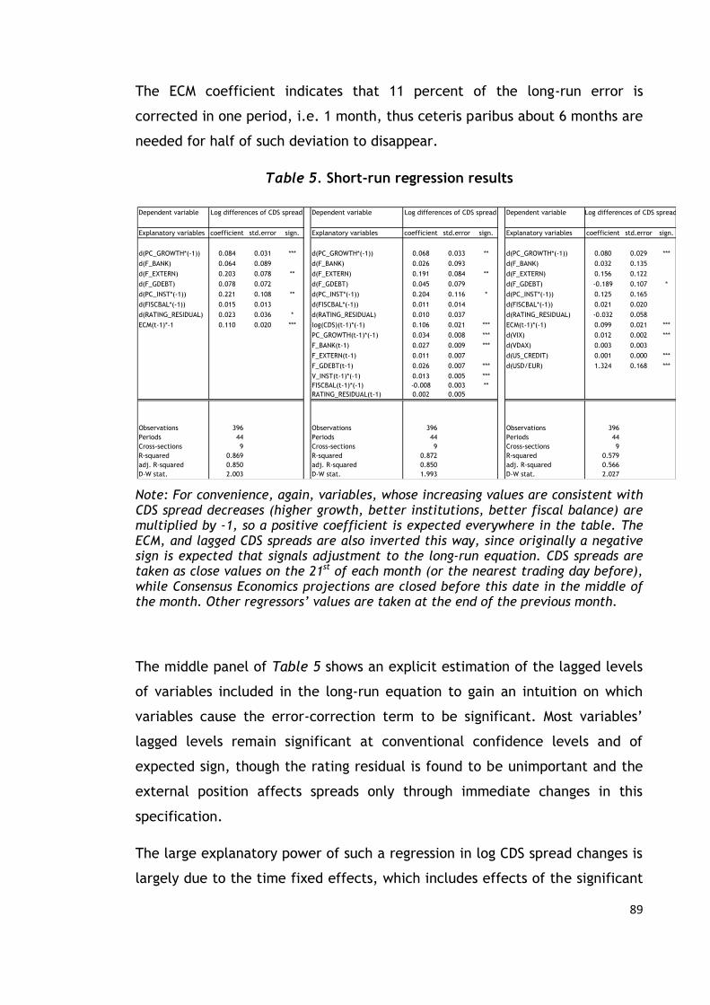
89

The ECM coefficient indicates that 11 percent of the long-run error is

corrected in one period, i.e. 1 month, thus ceteris paribus about 6 months are

needed for half of such deviation to disappear.

Table 5. Short-run regression results

Note: For convenience, again, variables, whose increasing values are consistent with CDS spread decreases (higher growth, better institutions, better fiscal balance) are multiplied by -1, so a positive coefficient is expected everywhere in the table. The ECM, and lagged CDS spreads are also inverted this way, since originally a negative sign is expected that signals adjustment to the long-run equation. CDS spreads are taken as close values on the 21st of each month (or the nearest trading day before), while Consensus Economics projections are closed before this date in the middle of the month. Other regressors’ values are taken at the end of the previous month.

The middle panel of Table 5 shows an explicit estimation of the lagged levels

of variables included in the long-run equation to gain an intuition on which

variables cause the error-correction term to be significant. Most variables’

lagged levels remain significant at conventional confidence levels and of

expected sign, though the rating residual is found to be unimportant and the

external position affects spreads only through immediate changes in this

specification.

The large explanatory power of such a regression in log CDS spread changes is

largely due to the time fixed effects, which includes effects of the significant

Dependent variable Dependent variable Dependent variable

Explanatory variables coefficient std.error sign. Explanatory variables coefficient std.error sign. Explanatory variables coefficient std.error sign.

d(PC_GROWTH*(-1)) 0.084 0.031 *** d(PC_GROWTH*(-1)) 0.068 0.033 ** d(PC_GROWTH*(-1)) 0.080 0.029 ***

d(F_BANK) 0.064 0.089 d(F_BANK) 0.026 0.093 d(F_BANK) 0.032 0.135

d(F_EXTERN) 0.203 0.078 ** d(F_EXTERN) 0.191 0.084 ** d(F_EXTERN) 0.156 0.122

d(F_GDEBT) 0.078 0.072 d(F_GDEBT) 0.045 0.079 d(F_GDEBT) -0.189 0.107 *

d(PC_INST*(-1)) 0.221 0.108 ** d(PC_INST*(-1)) 0.204 0.116 * d(PC_INST*(-1)) 0.125 0.165

d(FISCBAL*(-1)) 0.015 0.013 d(FISCBAL*(-1)) 0.011 0.014 d(FISCBAL*(-1)) 0.021 0.020

d(RATING_RESIDUAL) 0.023 0.036 * d(RATING_RESIDUAL) 0.010 0.037 d(RATING_RESIDUAL) -0.032 0.058

ECM(t-1)*-1 0.110 0.020 *** log(CDS)(t-1)*(-1) 0.106 0.021 *** ECM(t-1)*(-1) 0.099 0.021 ***

PC_GROWTH(t-1)*(-1) 0.034 0.008 *** d(VIX) 0.012 0.002 ***

F_BANK(t-1) 0.027 0.009 *** d(VDAX) 0.003 0.003

F_EXTERN(t-1) 0.011 0.007 d(US_CREDIT) 0.001 0.000 ***

F_GDEBT(t-1) 0.026 0.007 *** d(USD/EUR) 1.324 0.168 ***

V_INST(t-1)*(-1) 0.013 0.005 ***

FISCBAL(t-1)*(-1) -0.008 0.003 **

RATING_RESIDUAL(t-1) 0.002 0.005

Observations 396 Observations 396 Observations 396

Periods 44 Periods 44 Periods 44

Cross-sections 9 Cross-sections 9 Cross-sections 9

R-squared 0.869 R-squared 0.872 R-squared 0.579

adj. R-squared 0.850 adj. R-squared 0.850 adj. R-squared 0.566

D-W stat. 2.003 D-W stat. 1.993 D-W stat. 2.027

Log differences of CDS spreadLog differences of CDS spread Log differences of CDS spread

90

risk pricing component of spreads. Without time fixed effects the explained

variance of CDS spread changes would drop to around 10 percent. In the right

hand panel we show the estimate of the model using common proxies of

global risk appetite and global liquidity (VIX, VDAX indices, EU/USD rate and

the Baa-Aaa US corporate spread). The results confirm the importance of risk

appetite in affecting CDS spread changes, although these proxies cannot fully

capture all time-specific effects as shown by the relative lower explanatory

power of the regression compared to our benchmark time fixed effects

specification in the left panel of Table 5.

Fundamental variables affect CDS spreads in this regression mainly through

the long-term adjustment term. Of the fundamental variables only expected

growth, PC_GROWTH, is significant in differences at the 5 percent level. A

regression (not shown here) that includes the growth variable’s two

components, the regional average growth and the deviation from the regional

average (the cross-section specific part), results in only the regional average

part remaining significant. This indicates that changes in expected growth are

significant in such a short-run equation only due to their ability to proxy the

general growth outlook.

Our findings are consistent with the main results of the literature on sovereign

spreads. It is predominantly a time-varying common risk factor that explains

the changes of CDS spreads. This risk factor does however have a

“fundamental” component, the general growth outlook, whose changes are

able to explain some of the shocks to time-specific risk pricing. Fundamental

country-specific factors enter spreads mainly through an error-correction

term suggesting the importance of the long-run relationship between relative

spreads and relative fundamentals. Expectations on growth and external

positions are significant in such a relationship, but also government debt

ratios and a general development factor also related to EU membership,

institutional strength and political stability are important determinants45.

45 However we think that institutional strength and political stability are not on the same

importance in the case of developed and less developed countries. The difference between

91

III.4.2. Have the aspects of differentiation between countries

changed through time?

Several papers in the literature (Mody [2009]; Bernoth & Erdogan [2010];

Aizenman et al. [2011]; D’Agostino & Ehrmann [2013]) emphasized the time-

varying nature of the relationship between sovereign spreads and explanatory

variables. While a more refined approach would be a direct incorporation of

time-variation into the model, here we resort to simple rolling window

regressions on one- and two-year fixed-length windows.

Appendix 3 Figure 10 and Figure 11 plot coefficient point estimates and their

2 standard error bounds on the two window lengths. Although there are

notable differences, some general results stand out. On one hand, the

coefficient of growth decreases to a fraction of its initial value. In contrast,

the coefficients of factors representing the stability of the banking sector, the

“flow-type” external position variables and government debt ratios increase.

The institutional-political variable’s coefficient remains of similar magnitude

and of high significance throughout the period, while the fiscal balance

variable and the rating residual are insignificant or on the border of

insignificance throughout the sample.

Variables’ standard deviations are different (relative to each other and

through time), thus coefficient estimates’ changes does not say anything

about how the relative importance of these variables changed in explaining

the CDS spread. To gain an intuition on this concept we calculate and plot the

following measure. For each time window and each explanatory variable we

calculate the difference between the R-squared of the full model and the R-

squared of a restricted regression that excludes the given variable. Variables,

which are important in explaining the levels of CDS spreads in the region,

contribute more to the explanatory power of the model.

the institutional strength and political stability of two developed countries might cause a less

significant difference in CDS spreads, then a difference of two developing countries.

92

Figure 3. Explanatory power differences of restricted and unrestricted

long-run regressions

Note: 1-year rolling windows. Dates indicated are ending dates of the

estimation window.

Contributions to the explanatory power of regressions suggest similar

processes as coefficients’ evolutions (Figure 3). We observe a decrease of

explanatory power of the growth outlook variable during the period, while

government debt, banking system stability, external balance factors have

become significantly more important in the CDS spreads regressions over

time. The institutional-political variable has been significant throughout the

sample, while rating residuals and fiscal balance outlook have not added

much explanatory power.

These results imply that time-variation of variables’ effects were important in

Eastern Europe during the crisis. Moreover, considering that the Eurozone

periphery’s sovereign crisis brought issues of government debt, banking

system stability and external balances into the center of attention, the

findings that these factors gained relative importance suggests wake-up call

effects.

0

0.1

0.2

0.3

0.4

0.5

0.6

0.7

Sep/2008

Nov/

2008

Jan/2009

Marc

h/2009

May/

2009

July

/2009

Sep/2009

Nov/

2009

Jan/2010

Marc

h/2010

May/

2010

July

/2010

Sep/2010

Nov/

2010

Jan/2011

Marc

h/2011

May/

2011

July

/2011

Sep/2011

Nov/

2011

Jan/2012

Marc

h/2012

PC_GROWTH F_BANK F_EXTERN F_GDEBT

PC_INST FISCBAL RATING_RESIDS

93

III.4.3. Robustness checks

We perform several robustness checks to see how sensitive results are. First,

regressions are re-estimated on quarterly data to see whether linear

interpolation of variables had a significant affect. A priori we would expect

the banking stability factor and the component of development-institutions-

politics to be possibly affected as these are constructed by the use of (also)

linearly interpolated variables. Growth, external position, fiscal balance and

ratings are on the other hand dominantly based on either Bloomberg data

(available daily), or on projections of Consensus Economics (available on a

monthly basis). Since on quarterly frequency we have less observations we

expect coefficient uncertainty to be larger.

Appendix 4 Table 9 shows the results of quarterly regressions. The only

material difference in the long-run equation compared with the baseline

model is the insignificance of the fiscal balance variable (which is available

monthly). Otherwise standard errors are systematically higher, as expected.

The short-run equation estimates are also similar to those in the monthly

case. One key difference, however, is the larger coefficient of the error-

correction term. Much of this difference is reasonable: since time intervals

are longer between two observations in the quarterly data set, therefore to

represent a long-term effect of similar magnitude the coefficient of the ECM

term has to increase more than three-fold.

We next turn to the issue of cross-section heterogeneity of results. Since we

have a low number of time series observations even on the monthly frequency

and as suggested before coefficients are also varying over time, it is not

possible to estimate regressions separately for each country. We therefore

restrict ourselves to estimating the model on two subsamples, and then we

turn to comparing results of the panel data set of 13-countries to gain an

intuition on how stable results are to cross-section selection.

Appendix 4 Table 9 shows coefficient estimates on the two subsamples. We

chose to split the sample based on the relative value of stock variables, with

regressions estimated for a subsample of countries of worse initial

94

fundamentals (Bulgaria, Latvia, Hungary, Turkey) and another subsample of

the remaining five countries, where stock-type variables were relatively

better (Croatia, Czech Republic, Lithuania, Poland, Russia).

Although most coefficients remain significant and of expected sign in the long

run regression, there are some differences in coefficients worth mentioning.

Compared to the baseline model the bank variable has a significantly larger

parameter in the countries with better stocks, whereas the government debt

variable loses significance. In the subsample of countries with worse

fundamentals external position, government debt and ratings have greater

parameters than in the benchmark estimation. In the short-run equation the

relative CDS spreads of countries with better fundamentals are found to be

more affected by changes of fundamentals and less so by the error-correction

term compared with the other subsample’s estimates.

The data set of the larger cross-section also results in somewhat different

coefficient estimates for some variables. Notably, in the long-run equation

government debt becomes insignificant, while the coefficients of growth and

ratings are significantly larger. This may either result from the difference of

the cross-section or from the smaller variable set in this panel. To find out,

we estimate the model using the smaller variable set on the cross-section of 9

countries. In the case of the growth variable, this estimation results in a

similarly large parameter as in the 13-country panel, which implies that the

smaller variable set seems to be the reason of the deviation from the

benchmark model. In the case of government debt, however, the coefficient

is similar to the benchmark case, suggesting that in this case the addition of

the four new countries caused the difference between the two panels.

Ratings’ parameter differs due to a blend of the two reasons. The rating

regression residuals seem to take up larger coefficients to explain spreads

when government debt loses significance due to the cross-section differences,

but they are also larger owing to the difference in the variable set. The lower

coefficients of rating residuals in the benchmark regression also suggests that

the used 9-country panel’s variable set has a significant informational

advantage relative to the variable set of larger cross-section.

95

To sum up experiences of cross-section heterogeneity, some parameters, such

as institutions in the long-run equation and changes in the prospects for

growth and the external position, as well as the ECM term seem to be stable

explanatory variables in the model with coefficients largely similar across

different estimation samples. However changes to the sample leads to

significant impacts of parameters in some cases for growth, bank stability and

the debt variable in the levels equation.

Finally, and in view of the cross-section heterogeneity that we find for some

variables, we compare regressions estimated on samples including and

excluding Hungary. The reason for such an exercise is to assess how relevant

results are in an out-of-sample context: namely if the relationship between

relative CDS spreads and fundamentals estimated for other Eastern European

countries provides a good estimate for such a relationship in the Hungarian

case. Results presented in Appnedix 4 Table 10 are reassuring in this respect.

Both long-run and short-run equations have similar estimates with and without

Hungary for the full time sample and the subsample estimated on 2010-2012

data, although government debt’s coefficient increases even more in the

latter sample when Hungary is not in the sample.

III.5. Conclusions

We study the relationship between relative sovereign CDS spreads and relative

country-specific fundamentals. Principal components and factors are

extracted from a wide array of fundamental variables encompassing

expectations of growth, fiscal and external balances and actual data on the

banking sector, government debt position, as well as indicators assessing the

institutional strength and political stability of countries. The sample of the

data is the Eastern European region in the period between July 2008 and

March 2012. Time fixed effect panel regressions of both levels and first

differences are estimated between CDS spreads and fundamental variables,

with an error-correction mechanism linking levels to the short-run equation.

96

In agreement with previous studies, we find that lower expected growth,

weaker external balances, higher government debt ratios are associated with

higher sovereign CDS spreads. Consistent with the recent literature, the

indicators of banking sector stability are found to be important in explaining

spreads. We show that explicit proxies of institutional and political factors,

which are rarely used in related studies, also have a significant impact. In

contrast with much of the literature, however, we do not find a positive

relationship between the level of fiscal deficit and CDS spreads, which may be

a result of the sample and of reverse causality between credit risk and fiscal

balance.

According to the regression of variable changes, relative fundamentals affect

CDS spreads mainly through an error-correction term contradicting standard

theory, which predicts immediate reaction of markets to new information.

The significance of the error-correction term may be due to the activity of

fund managers, who, owing to the time cost of information collection and

market liquidity reasons, adjust portfolios only gradually.

Some coefficients seem to be sensitive to selection of the country sample.

Time-variation of parameters is supported by simple rolling regressions,

pointing to an increase of government debt, banking stability and external

balance in the assessment of relative riskiness of countries. This may be a

result of a wake-up call effect from the sovereign crisis of the Eurozone

periphery.

97

IV. APPLICATION TO THE HUNGARIAN CDS SPREAD

This part is a case study about the change in the Hungarian relative CDS

spread. As far as we know, this part provides the most in-depth analysis of

the country-specific fundamental determinants of the Hungarian CDS

spread so far.

The model discussed in the previous part attributes the Hungarian CDS

spread’s relative increase to both a worsening of fundamentals (growth

prospects and banking stability) and to a changing in investor preferences:

government debt, one of the country’s key weaknesses, has become more

important in relative sovereign risk assessment.

The estimations were also carried out for three other regional countries

(Poland, Russia, and Turkey). The results are presented in Appendices 6-8:

Figures 12-26.

IV.1. Introduction, stylized facts

Since the beginning of our sample in July 2008, Hungarian 5-year CDS spreads

have increased from near 100 basis points to over 500 basis points in March

2012, when our sample ends. Spreads first shot above 500 basis points after

the bankruptcy of Lehman Brothers, when the crisis spread to emerging

markets. The whole region was affected by that risk premium shock, and the

Hungarian CDS spread rose roughly together with the regional average.

Eastern European indicators experienced another peak in early 2009, but then

a region-wide decline followed in most of 2009. In spring and summer 2010,

Hungarian CDS spreads increased again, however, this time it was an increase

of mostly country-specific origins: the average of Eastern European CDS

spreads remained largely stagnant until 2011 summer.

In mid-2011 fears of the euro area sovereign crisis spreading to Italy and the

euro area banking sector, as well as concerns related to a Greek default, in

the autumn, led to a new round of CDS spread increases in the region. The

Hungarian indicator was proportionately more affected and its difference

98

compared to the regional average has increased to 300 basis points by which

time it was around double the Eastern European average (Figure 4).

Expectations of a Greek-IMF-EU agreement and the bond swap acted to

reduce Hungarian and other Eastern European spreads in the last months of

the sample period.

Figure 4. Hungarian 5-year CDS spreads and the Eastern European average

(July 2008 – March 2012)

In terms of variables incorporated in our model, the logarithm of Hungarian

CDS spread compared to the mean of Eastern European logarithmic CDS

spreads began to deviate from near 0 levels in end-2009, early-2010 and

increased to a value of 0.8 by the end of the sample.

Based on fundamental variables (Figure 5) Hungary had a relative worse

growth outlook, banking stability and a significantly worse government debt

position than the regional average in the whole period. Moreover the growth

variable and the factor representing banking sector vulnerability deteriorated

during the period, which are thus candidates for explaining the worsening of

the relative spread. On the other hand Hungary has been significantly better

-100

0

100

200

300

400

500

600

700

-100

0

100

200

300

400

500

600

700

July

/2008

Sep/2008

Nov/

2008

Jan/2009

Marc

h/2009

May/

2009

July

/2009

Sep/2009

Nov/

2009

Jan/2010

Marc

h/2010

May/

2010

July

/2010

Sep/2010

Nov/

2010

Jan/2011

Marc

h/2011

May/

2011

July

/2011

Sep/2011

Nov/

2011

Jan/2012

Marc

h/2012

Difference between Hungary and regional average (basis points)

Hungarian CDS spread (basis points)

Regional average CDS spread (basis points)

99

than regional peers on the grounds of the institutional-political-development

component proxied by the variable, PC_INST. Also, the prospects of external

balance were better and has improved compared to the region in the period.

In terms of credit ratings, Hungary was initially better than the regional

average but this has changed during the sample. Fundamentals partly

explained the deterioration since the rating residual rose by a smaller extent

than relative ratings themselves. Yet there has been a notable rise in this

factor as well, which indicates the importance of factors which our rating

regressions were not able to capture.

Figure 5. Hungarian indicators compared to regional averages

Note: Variables are scaled so that increases are consistent with a

deterioration of credit risk. Similar figures for the other countries in the

sample are shown in Appendix 9 Figures 27-35.

-0.2

0.0

0.2

0.4

0.6

0.8

1.0

July

/2008

Oct

/2008

Jan/2009

Apr/

2009

July

/2009

Oct

/2009

Jan/2010

Apr/

2010

July

/2010

Oct

/2010

Jan/2011

Apr/

2011

July

/2011

Oct

/2011

Jan/2012

PC_GROWTH

PC_GROWTH

0.0

0.2

0.4

0.6

0.8

1.0

1.2

July

/2008

Oct

/2008

Jan/2009

Apr/

2009

July

/2009

Oct

/2009

Jan/2010

Apr/

2010

July

/2010

Oct

/2010

Jan/2011

Apr/

2011

July

/2011

Oct

/2011

Jan/2012

F_BANK

F_BANK

-0.9

-0.8

-0.7

-0.6

-0.5

-0.4

-0.3

-0.2

-0.1

0.0

July

/2008

Oct

/2008

Jan/2009

Apr/

2009

July

/2009

Oct

/2009

Jan/2010

Apr/

2010

July

/2010

Oct

/2010

Jan/2011

Apr/

2011

July

/2011

Oct

/2011

Jan/2012

F_EXTERN

F_EXTERN

0.0

0.5

1.0

1.5

2.0

2.5

July

/2008

Oct

/2008

Jan/2009

Apr/

2009

July

/2009

Oct

/2009

Jan/2010

Apr/

2010

July

/2010

Oct

/2010

Jan/2011

Apr/

2011

July

/2011

Oct

/2011

Jan/2012

F_GDEBT

F_GDEBT

-3.0

-2.5

-2.0

-1.5

-1.0

-0.5

0.0

July

/2008

Oct

/2008

Jan/2009

Apr/

2009

July

/2009

Oct

/2009

Jan/2010

Apr/

2010

July

/2010

Oct

/2010

Jan/2011

Apr/

2011

July

/2011

Oct

/2011

Jan/2012

PC_INST

PC_INST

-4.0

-3.0

-2.0

-1.0

0.0

1.0

2.0

3.0

4.0

July

/2008

Oct

/2008

Jan/2009

Apr/

2009

July

/2009

Oct

/2009

Jan/2010

Apr/

2010

July

/2010

Oct

/2010

Jan/2011

Apr/

2011

July

/2011

Oct

/2011

Jan/2012

FISCBAL

FISCBAL

-1.5

-1.0

-0.5

0.0

0.5

1.0

1.5

2.0

July

/2008

Oct

/2008

Jan/2009

Apr/

2009

July

/2009

Oct

/2009

Jan/2010

Apr/

2010

July

/2010

Oct

/2010

Jan/2011

Apr/

2011

July

/2011

Oct

/2011

Jan/2012

RATINGS

RATINGS

-1.5

-1.0

-0.5

0.0

0.5

1.0

1.5

July

/2008

Oct

/2008

Jan/2009

Apr/

2009

July

/2009

Oct

/2009

Jan/2010

Apr/

2010

July

/2010

Oct

/2010

Jan/2011

Apr/

2011

July

/2011

Oct

/2011

Jan/2012

RATING_RESIDS

RATING_RESIDS

-0.2

0.0

0.2

0.4

0.6

0.8

1.0

July

/2008

Oct

/2008

Jan/2009

Apr/

2009

July

/2009

Oct

/2009

Jan/2010

Apr/

2010

July

/2010

Oct

/2010

Jan/2011

Apr/

2011

July

/2011

Oct

/2011

Jan/2012

log CDS spread

log CDS spread

100

IV.2. Model explanations for the deterioration

To apply results of the model we turn to the long-run equation to assess how

relative fundamentals have explained relative Hungarian CDS spreads. Figure

6 plots the observed and model-based estimates for the relative CDS spread

throughout the sample. Since results have suggested a time-varying property

of coefficients we also calculated and plotted the expected value of the

Hungarian relative CDS spread based on estimates of the 2010-2012

subsample.

Figure 6. Relative CDS spreads

The figure shows that, on the whole, the observed Hungarian CDS spread was

relatively close to the values implied by fundamentals and the model. A large

part of the spread’s deterioration was also consistent with a worsening of

fundamental variables. Based on full sample estimates, CDS spreads were

-0.6

-0.4

-0.2

0.0

0.2

0.4

0.6

0.8

1.0

July

/2008

Sep/2008

Nov/

2008

Jan/2009

Marc

h/2009

May/

2009

July

/2009

Sep/2009

Nov/

2009

Jan/2010

Marc

h/2010

May/

2010

July

/2010

Sep/2010

Nov/

2010

Jan/2011

Marc

h/2011

May/

2011

July

/2011

Sep/2011

Nov/

2011

Jan/2012

Marc

h/2012

Observed and model-based values of the relative Hungarian CDS spread

CDS deviation from regional mean

expected difference based on fundamentals (full period)

expected difference based on fundamentals (2010-2012)

101

somewhat lower before 2010 than expected based on the model, and were

higher than model estimates after this period.

Figure 7 shows the contributions of various fundamentals variables to the

model-based value of the dependent variable (full sample estimates). Relative

high government debt stands out as the primary factor worsening the

Hungarian CDS spread compared to the region, while the main factor reducing

the CDS spread is the effect of better institutions. Banking stability and to a

lesser extent the periodically inferior growth prospects contributed to

explaining Hungary’s higher CDS spread, while the better external balance

moderated the indicator. The effect of fiscal balance and rating residuals on

the level of relative CDS spreads seems unimportant compared to other

factors. It is also clear that increases of values (denoting a relative

deterioration) of the growth and bank variables have been the main culprits in

worsening CDS spreads. A relative improvement of external balances could

only lessen the CDS increase.

102

Figure 7. Contributions to the model-based value of the relative CDS

spread

As shown earlier in Figure 6, Hungarian relative CDS spreads were higher than

model-based values after mid-2010 if we calculate with the full sample’s

coefficients, but were largely in-line with the model-implied values if we look

at 2010-2012 estimates. This points to another key factor in the increase of

relative CDS spreads, that of shifts in variables’ coefficient estimates, i.e.

changes in CDS spreads’ sensitivity to variables over time. As we have seen in

the previous section, mainly those variables’ coefficients have increased,

which were relevant in terms of the crisis of the Eurozone periphery, i.e.

government debt and banking stability variables, suggesting a wake-up call

effect. Unfortunately, exactly these variables happened to be relative

weaknesses of Hungary compared to Eastern European peers.

103

To quantify the two distinct effects on the relative Hungarian CDS spread, i.e.

the worsening of fundamentals and the shift in investor preferences (the

wake-up call effect), we use the Oaxaca-Blinder decomposition (Blinder

[1973]; Oaxaca [1973]). In particular we decompose the difference between

the model-implied value for March 2012 due to the 2010-2012 period

estimates (CDSp2 = 0.69) and the model-implied value for January 2010 due to

the full sample estimates (CDSfull = 0.2).

Applied to our context the Blinder-Oaxaca decomposition separates the effect

of changing parameters,

, and changing variables, , so that:

(8)

where

and

denote the full sample and the second period (2010-2012)

estimates, and stand for fundamental variable values in March 2012 and

January 2010, respectively.

Figure 8 presents the result of such decomposition. The approximate increase

of 0.5 in the model-implied values of the relative Hungarian CDS spread due

to the different estimates and time periods is mainly the result of worsening

relative growth outlook and banking stability on the one hand, and a large

increase in government debt’s parameter, i.e. a wake-up call effect, on the

other.

104

Figure 8. Fundamental and wake-up call effects in changes of Hungarian

spreads

In the above reasoning we referred to implications of the long-run equation

and have neglected model dynamics. We end this subsection with a brief

account of how the above mentioned effects translate into (model-implied)

changes of the Hungarian spread. The worsening of fundamentals has two

effects. On one hand it can immediately impact Hungarian CDS spreads

through the coefficients of fundamental variables’ changes. We have seen

however that these effects are relatively small. The other channel is the

increase of the model-implied CDS spread level, which causes the error-

correction term to affect CDS spread changes gradually over time.

Similarly, the wake-up call affects spreads mainly by increasing the model-

implied CDS spread level. In the Hungarian case and after 2010 the long-run

equation estimates of the full sample implied a lower CDS spread than which

has been observed in the market. This would have caused the error-correction

mechanism to exert a downward pressure on Hungarian CDS spreads in the

short-run equation. However due to changes in investor preferences the

-0.10

-0.05

0.00

0.05

0.10

0.15

0.20

0.25

0.30

PC

_G

RO

WT

H

F_BA

NK

F_EXT

ER

N

F_G

DEBT

PC

_IN

ST

FIS

CBA

L

RA

TIN

G_R

ESI

D

effect of fundamental changewake-up call effecttotal impact on relative CDS change

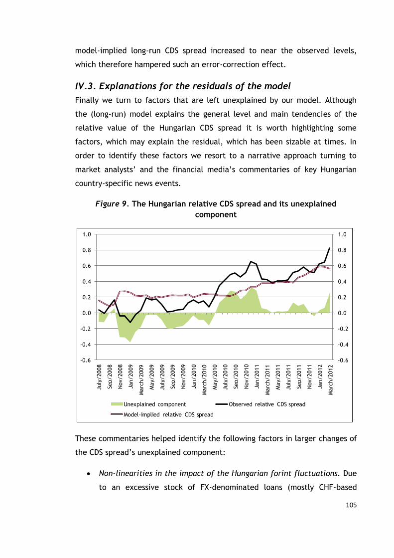
105

model-implied long-run CDS spread increased to near the observed levels,

which therefore hampered such an error-correction effect.

IV.3. Explanations for the residuals of the model

Finally we turn to factors that are left unexplained by our model. Although

the (long-run) model explains the general level and main tendencies of the

relative value of the Hungarian CDS spread it is worth highlighting some

factors, which may explain the residual, which has been sizable at times. In

order to identify these factors we resort to a narrative approach turning to

market analysts’ and the financial media’s commentaries of key Hungarian

country-specific news events.

Figure 9. The Hungarian relative CDS spread and its unexplained

component

These commentaries helped identify the following factors in larger changes of

the CDS spread’s unexplained component:

Non-linearities in the impact of the Hungarian forint fluctuations. Due

to an excessive stock of FX-denominated loans (mostly CHF-based

-0.6

-0.4

-0.2

0.0

0.2

0.4

0.6

0.8

1.0

-0.6

-0.4

-0.2

0.0

0.2

0.4

0.6

0.8

1.0

July

/2008

Sep/2008

Nov/

2008

Jan/2009

Marc

h/2009

May/

2009

July

/2009

Sep/2009

Nov/

2009

Jan/2010

Marc

h/2010

May/

2010

July

/2010

Sep/2010

Nov/

2010

Jan/2011

Marc

h/2011

May/

2011

July

/2011

Sep/2011

Nov/

2011

Jan/2012

Marc

h/2012

Unexplained component Observed relative CDS spread

Model-implied relative CDS spread

106

mortgage loans) in Hungary46, the weakening of the currency has the

potential to hit the Hungarian economy and the banking sector

disproportionally more than other countries in the region. Especially as

the exchange rate of the forint approaches levels that market

participants identify as a danger zone, non-linear effects between the

exchange rate and the CDS spread arise. While the model is able to

explain spread movements due to a deterioration of the growth

outlook, which regularly has taken place in these periods of financial

instability (early 2009, mid-end-2011) and the logarithmic specification

of the spread in the model helps to account for some of the non-

linearities, clearly the model lacks in explaining the full sovereign

credit risk impact of exchange rate deterioration. Two main reasons

may be tail risks to the growth and fiscal outlook that are not captured

by the base case projections of economists surveyed by Consensus

Economics, and the impact of forward-looking expectations of banking

sector stability for which the actual data we have could be a poor

proxy. Non-linearities have in the past worked the other way around as

well. Once improving international and domestic conditions caused the

forint to move away from the perceived danger zone, Hungary’s

spreads improved relatively more than the model’s prediction (e.g. in

the summer of 2009).

Sudden shift in households’ exchange rate expectations. Related to the

previous point, households have added to some of the non-linearities

due to a change in their behavior regarding FX market activity. In

general, households have historically had a stabilizing impact on the

exchange rate of the Hungarian forint as in periods of exchange rate

depreciations they tended to increase their foreign currency holdings,

whereas they sold FX holdings when the forint strengthened. However,

unusually rapid episodes of HUF weakening seemed to alter this

46 A detailed paper about credit expansion and external financing needs in Hungary: (Király

et al. [2008]). Another paper about the banking sector’s external financing costs: (Páles &

Homolya [2011]).

107

sector’s behavior adding to the pace of forint depreciations (such as in

early 2009 and in January 2012).

News, statements about the IMF and other international agreements

(i.e. the ECB EUR/HUF FX swap line). According to market analysts’

opinions, in the period following the collapse of Lehman Brothers, a

key determinant of relative improvement of Hungary’s risk assessment

has been related to Hungary’s IMF program that ensured the financing

ability of the sovereign. This has been arguably important in a time

when even domestic auctions have failed. As we have observed in the

past years not only the changes to having such an international

financial safety net but also expectations of the possibility or of the

timing of such agreements have been important in influencing spreads

(breakup of agreement in July 2010 and December 2011; and hopes of

an agreement in November 2011 and in early-2012). Although these

factors are not explicitly built into our model, so normally we cannot

assess their quantitative impact, they may however enter though the

rating residual, if credit rating agencies downgrade/upgrade the

country due to this factor.

Impact of political statements. Market participants have occasionally

reacted significantly to politician’s statements. In recent years several

episodes could be identified including both positive (e.g.

announcement of the Orbán-Barosso agreement, April 2012) and

negative (e.g. statements about a potential default of Hungary, June

2010) effects. Although we do have variables grasping domestic politics

incorporated in our variable PC_INST, this measure is unable to pick-up

such high-frequency market movements for most of these variables are

available on annual frequency and also since they rather refer to

general political stability.

Market assessment of government fiscal measures. Even though our

model incorporates the impact of government fiscal measures’

announcements through impacting the growth and fiscal outlook

projections, these variables may not be able to capture the indirect

108

effects that measures have on market confidence toward the

government. Both negative and positive events can be mentioned in the

last years: the Hungarian CDS spread significantly declined around the

time of the announcement of the Széll Kálmán Plan (February-March

2011), which, judging from market commentaries, was seen as an

important step not only from the perspective of balancing the budget,

but also in the aspect of the government taking a market-friendly path.

On the negative side government announcements such as the

introduction and the augmentation of the bank levy (June 2010), the

regulatory changes regarding the private pension funds, the sectoral

taxes and the early mortgage repayment scheme (October 2010)

negatively impacted Hungarian risk assessment.

IV.4. Conclusion

In the case of Hungary our model is able to reasonably explain both the level

and the general trends of the CDS spread compared to the Eastern European

region. Regarding the Hungarian relative CDS spread levels, the high

government debt ratio and, increasingly, the poor banking sector stability,

stand out as main factors of a higher spread, while based on relative

development-institutions-political stability and the external balance the

country would have a lower than average CDS spread.

The deterioration of the Hungarian indicator compared to the region observed

since end-2009 and early-2010 is the consequence of two reasons. On one

hand it is due to the worsening of relative fundamentals, in particular the

growth outlook and banking stability. On the other hand, however, it seems to

be a result of bad luck: investors have in the past years given a larger weight

to government debt ratios in their relative risk assessment, which turns out to

be Hungary’s key weakness compared to regional peers.

109

V. SUMMARY

The goal of Part II was to compare the two most commonly used auction

techniques (discriminatory and uniform price auctions) through the summary

of the relevant literature. Among several other countries, Poland has changed

its auction method on the T-bond and T-bill markets from the previously used

discriminatory format to the uniform price formula (the change was

implemented on January 1, 2012). In Hungary, both the ÁKK (in the case of T-

Bonds and T-bills) and the MNB (in the case of FX, FX-swaps, and Credit

auctions) still use the discriminatory format. The most important goal of the

analysis was to review the arguments for and against the different formulas.

The literature about the allocation of the issued bonds analyses the

different formulas (uniform and the discriminatory auctions) mostly from the

perspective of the expected revenue of the issuer. While in the case of single-

unit auctions (for example art masterpiece), the second price and the first

price auctions result in the same expected revenue, this theorem cannot be

universalized for the (in the case of securities) relevant multi-unit (uniform

price and discriminatory) auctions.

In the simplest multi-unit model the aggregate demand curve is higher in

the case of uniform price auctions; while in the case of the discriminatory

method, the average price of the accepted bids is increased by the presence

of price discrimination. The main results of further models are that on the

one hand, the uniform price auction is able to stimulate the participation of

the bidders with smaller analyzing capacity; but on the other hand it gives

more opportunity for the manipulation of prices and cartels. Therefore, the

two formulas cannot be ranked on the basis of theoretical models.

The theoretical results about the bidding behavior in the case of the two

methods are confirmed by both laboratory and real-life empirical evidence.

Those observations where the different auction formulas could be compared

in real-life auctions (because the auction format of a security was changed

110

from a given date, or two similar securities were auctioned in the same time

but with different methods) showed almost in every case that the use of the

uniform price formula results in a lower cost of several basis points.

However, all real-life experiments have been plagued by the identification

problem, that is, the change caused by the auction method is difficult to tell

apart from the effects of other circumstances. It would be a real scientific

breakthrough, though, to set up a real-life experiment in which the same

product would be sold simultaneously on both uniform-price and

discriminatory auctions. Even though fewer conclusions could be drawn than

in the previously proposed arrangement (due to the repetition of auctions), it

would be instructive to see an experiment where primary market actors have

to submit bids for both auction formats, then the real format would be

decided by drawing lots. We should note, however, that the experiment may

increase the ‘fog of war’, i.e. the strategy space may become even more

complicated and the number of possible equilibria may increase to extreme

heights. Such an experiment could be a very important step in future work;

however, it has to be supported by a bond issuer.

Despite the empirical evidence of a lower expected revenue in the

discriminatory auction case, the majority of national treasuries are using the

discriminatory formula, and the central bank instruments are also typically

issued by using this method. This can be explained by the fact that issuers

might not only consider the expected revenue, but also other factors as well

(for example the lower expected volatility in the case of discriminatory

auctions).

The main advantages of the uniform price auction method might be: higher

expected revenue, low markup between the market price and the auction

price (in the long-term average), and increased participation in the auctions.

The discriminatory auctions are able to reduce volatility, reveal better the

true valuations, and hinder price-manipulations.

111

In the case of central bank instruments, the orientation of the market price

might be an important goal. Whether the discriminatory or the uniform price

auction is the better method in this aspect is still a question. This is difficult

to answer because the reviewed literature has not examined this issue. As

there is no empirical study available, we should take a theoretical approach

to resolve this problem. Market price is probably best oriented if there are

more participants or high-volume bids in the auction, in which case the

auction price may have a greater impact on the secondary market as well.

The problem of bidders may be interpreted as a private-value auction (i.e.,

not as a common-value auction frequently studied in literature), that is,

bidders do not ask the simple question of how to win instruments below the

post-auction market price. Instead, banks would like to obtain cheaper funds

even if they have to pay the price of reputation risk (‘stigma effect’ that can

be evaluated bank by bank because participation in FX swap and central bank

credit auctions may be seen as a sign of difficulties in raising funds in the

money market, which may raise the risk premium of the bank concerned).

This problem may turn the entire auction into a private-value auction due to

the private valuation of the reputation loss. Assuming risk aversion, a private-

value auction may result in bids being submitted at discriminatory-price

auctions even at a smaller ‘expected financial gain – reputation loss’

difference because the price a bank paid for the funds if their bid is accepted

will be known. In contrast, in the case of uniform-price auctions, the high

degree of ‘fog of war’ means that bidders may be uncertain about the bid

price and less clear about the expected financial gain. The above reasoning

relies on a large number of assumptions. Consequently, more studies and

model experiments would be needed on the subject of the orientation of

market prices.

In the case of central bank instruments currently sold at auctions (one-

week and three-month FX-swaps, six-month variable interest rate

collateralized loans, FX-auctions) the orientation of the market price may be

important, and several factors may need to be taken into account. Overall,

for the time being there seems to be no strong argument for the adoption of

112

the uniform-price format, so in line with the international practice of central

banks, discriminatory-price auctions may continue to be appropriate

allocation mechanisms.

In the case of the auction of Hungarian government bonds, maximizing the

expected revenue of the issuer may also be important. In this respect the

overwhelming majority of empirical evidence shows that uniform-price

auctions have an advantage of a few basis points or at least the average profit

of bidders was lower in uniform-price auctions in most of the cases reviewed.

It should be noted, however, that discriminatory auctions may be more

advantageous in an uncertain market environment or where the bid-to-cover

ratio is low. Consequently, amidst the present uncertainties, switching to the

uniform-price format could be hazardous. Changing the auction format (or

conducting an experiment into such a change) would be relevant if volatility

remained persistently low with consistently high bid-to-cover ratios. However,

the adoption of the uniform-price format may be worth considering under

better market conditions in the hope of cheaper funding. In order to suppress

the possibility of manipulation, in the uniform-price system it is particularly

important for the issuer to be able to change the volume sold, and the success

of a switch depends to a large extent on the probability of the market entry

of smaller participants, thus also on the characteristics of the primary dealer

system. The publication of an in-depth study on the change implemented by

the Polish treasury in 2012 could shed light on important considerations for

the Hungarian auction system.

In Part III we study the relationship between relative sovereign CDS spreads

and relative country-specific fundamentals.

We adhere to the literature in assuming that most of the time series

variation in CDS spreads are a result of common shocks to the pricing of risk

and we concentrate the analysis on the other, cross-sectional aspect of CDS

spreads by assessing which fundamental factors have been empirically

important in explaining the relative riskiness of countries as proxied by the

relative magnitude of these indicators.

113

We lay emphasis on using a dataset that treats some empirical issues that,

in previous studies, have often been disregarded. First, where possible we use

projections of future variables instead of actual data (in line with D’Agostino

& Ehrmann [2013]). Second, we aim to reduce the adverse effects of variable

omissions by including a larger and a conceptually wider set of fundamental

variables than usual in similar studies. Besides the standard macroeconomic

variables, we incorporate data on the banking sector and use a set of political

and institutional variables as well. Principal components and factors are

extracted from conceptually similar variables’ groups and these are then used

in CDS spreads’ regressions to overcome problems of multicollinearity and the

curse of dimensionality. To further limit adverse effects of variable omission,

we attempt to make use of the extra information contained in credit ratings

compared to that in our fundamental variable set. A further output of this

research could be a methodological paper, in which the main question would

be, if our model can beat the mainstream models in this topic.

Principal components and factors are extracted from a wide array of

fundamental variables encompassing expectations of growth, fiscal and

external balances and actual data on the banking sector, government debt

position, as well as indicators assessing the institutional strength and political

stability of countries. The sample of the data is the Eastern European region

in the period between July 2008 and March 2012. Time fixed effect panel

regressions of both levels and first differences are estimated between CDS

spreads and fundamental variables, with an error-correction mechanism

linking levels to the short-run equation.

In line with previous studies, we find that lower expected growth, weaker

external balances and higher government debt ratios are associated with

higher sovereign CDS spreads. Consistent with the recent literature, the

indicators of banking sector stability are found to be important in explaining

spreads. We show that explicit proxies of institutional and political factors,

which are rarely used in related studies, also have a significant impact. In

contrast to much of the literature, however, we do not find a positive

relationship between the level of fiscal deficit and CDS spreads, which may be

114

a result of the sample and of reverse causality between credit risk and fiscal

balance.

According to the regression of variable changes, relative fundamentals

affect CDS spreads mainly through an error-correction term contradicting

standard theory, which predicts immediate reaction of markets to new

information. The significance of the error-correction term may be due to the

activity of fund managers, who, owing to the time cost of information

collection and market liquidity reasons, adjust portfolios only gradually.

Some coefficients seem to be sensitive to selection of the country sample.

Time-variation of parameters is supported by simple rolling regressions,

pointing to an increase of government debt, banking stability and external

balance in the assessment of relative riskiness of countries. This may be a

result of a wake-up call effect from the sovereign crisis of the Eurozone

periphery.

This part’s main contribution to the literature is in assessing the

fundamental factors relevant for Eastern European CDS spreads. Analysis of

sovereign bond spreads’ determinants do exist for the region but even that is

scarce and our study contributes to those in assessing a larger array of

relevant factors limiting problems of variable omissions.

In Part IV our model is able to reasonably explain both the level and the

general trends of the relative spread compared to the region. The high

government debt ratio and, increasingly, the poor banking sector stability,

stand out as main factors of a higher relative spread, while based on relative

development-institutions-political stability and the external balance the

country would have a lower than average spread.

Since the end of 2009 and early-2010 the observed worsening of the

Hungarian indicator compared to the region is the consequence of two

reasons. On the one hand it is due to the worsening of relative fundamentals,

in particular to the growth outlook and banking stability. On the other hand,

however, it seems to be a result of bad luck: investors have in the past years

115

given a larger weight to government debt ratios in their relative risk

assessment, which turns out to be Hungary’s key weakness compared to

regional peers.

In the upcoming weeks, a paper will be submitted to Economics of

Transition. This paper will be similar to Part IV, but the case studies will

investigate three big Eastern European economies, Poland, Russia and Turkey.

116

VI. APPENDICES

VI.1. Appendix 1: The Revenue Equivalence Theory

From: (Krishna, 2009, p. 28) “Proposition. Suppose that values are independently and identically distributed and all bidders are risk neutral. Then any symmetric and increasing equilibrium of any standard auction, such that the expected payment of a bidder with value zero is zero, yields the same expected revenue to the seller.

Proof. Consider a standard auction form, A, and fix a symmetric equilibrium β of A. Let mA(x)

be the equilibrium expected payment in auction A by a bidder with value x. Suppose that β is such that mA(0)=0. Consider a particular bidder—say, 1—and suppose other bidders are following the equilibrium

strategy β. It is useful to abstract away from the details of the auction and consider the

expected payoff of bidder 1 with value x and when he bids β(z) instead of the equilibrium bid

β(x). Bidder 1 wins when his bid β(z) exceeds the highest competing bid β(Y1), or equivalently, when z>Y1. His expected payoff is:

where as before G(z)≡F(z)N-1 is the distribution of Y1. The key point is that mA(z) depends on

the other players’ strategy β and z but is independent of the true value, x. Maximization results in the first-order condition

At an equilibrium it is optimal to report z=x, so we obtain that for all y

Thus,

since, by assumption, mA(0)=0. Since the right-hand side does not depend on the particular auction form A, this completes the proof” (Krishna, 2009, p. 28).

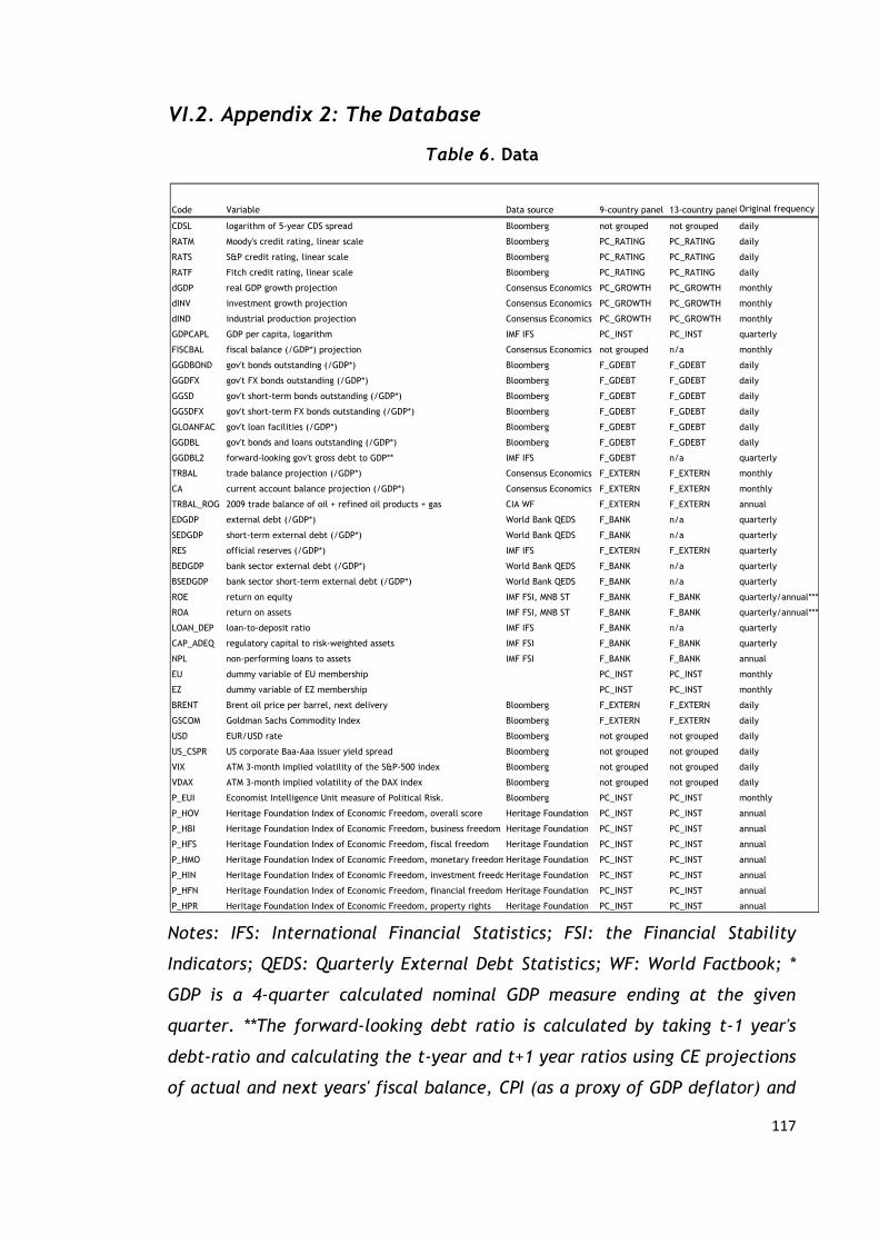
117

VI.2. Appendix 2: The Database

Table 6. Data

Notes: IFS: International Financial Statistics; FSI: the Financial Stability

Indicators; QEDS: Quarterly External Debt Statistics; WF: World Factbook; *

GDP is a 4-quarter calculated nominal GDP measure ending at the given

quarter. **The forward-looking debt ratio is calculated by taking t-1 year's

debt-ratio and calculating the t-year and t+1 year ratios using CE projections

of actual and next years' fiscal balance, CPI (as a proxy of GDP deflator) and

Code Variable Data source 9-country panel 13-country panelOriginal frequency

CDSL logarithm of 5-year CDS spread Bloomberg not grouped not grouped daily

RATM Moody's credit rating, linear scale Bloomberg PC_RATING PC_RATING daily

RATS S&P credit rating, linear scale Bloomberg PC_RATING PC_RATING daily

RATF Fitch credit rating, linear scale Bloomberg PC_RATING PC_RATING daily

dGDP real GDP growth projection Consensus Economics PC_GROWTH PC_GROWTH monthly

dINV investment growth projection Consensus Economics PC_GROWTH PC_GROWTH monthly

dIND industrial production projection Consensus Economics PC_GROWTH PC_GROWTH monthly

GDPCAPL GDP per capita, logarithm IMF IFS PC_INST PC_INST quarterly

FISCBAL fiscal balance (/GDP*) projection Consensus Economics not grouped n/a monthly

GGDBOND gov't bonds outstanding (/GDP*) Bloomberg F_GDEBT F_GDEBT daily

GGDFX gov't FX bonds outstanding (/GDP*) Bloomberg F_GDEBT F_GDEBT daily

GGSD gov't short-term bonds outstanding (/GDP*) Bloomberg F_GDEBT F_GDEBT daily

GGSDFX gov't short-term FX bonds outstanding (/GDP*) Bloomberg F_GDEBT F_GDEBT daily

GLOANFAC gov't loan facilities (/GDP*) Bloomberg F_GDEBT F_GDEBT daily

GGDBL gov't bonds and loans outstanding (/GDP*) Bloomberg F_GDEBT F_GDEBT daily

GGDBL2 forward-looking gov't gross debt to GDP** IMF IFS F_GDEBT n/a quarterly

TRBAL trade balance projection (/GDP*) Consensus Economics F_EXTERN F_EXTERN monthly

CA current account balance projection (/GDP*) Consensus Economics F_EXTERN F_EXTERN monthly

TRBAL_ROG 2009 trade balance of oil + refined oil products + gas CIA WF F_EXTERN F_EXTERN annual

EDGDP external debt (/GDP*) World Bank QEDS F_BANK n/a quarterly

SEDGDP short-term external debt (/GDP*) World Bank QEDS F_BANK n/a quarterly

RES official reserves (/GDP*) IMF IFS F_EXTERN F_EXTERN quarterly

BEDGDP bank sector external debt (/GDP*) World Bank QEDS F_BANK n/a quarterly

BSEDGDP bank sector short-term external debt (/GDP*) World Bank QEDS F_BANK n/a quarterly

ROE return on equity IMF FSI, MNB ST F_BANK F_BANK quarterly/annual***

ROA return on assets IMF FSI, MNB ST F_BANK F_BANK quarterly/annual***

LOAN_DEP loan-to-deposit ratio IMF IFS F_BANK n/a quarterly

CAP_ADEQ regulatory capital to risk-weighted assets IMF FSI F_BANK F_BANK quarterly

NPL non-performing loans to assets IMF FSI F_BANK F_BANK annual

EU dummy variable of EU membership PC_INST PC_INST monthly

EZ dummy variable of EZ membership PC_INST PC_INST monthly

BRENT Brent oil price per barrel, next delivery Bloomberg F_EXTERN F_EXTERN daily

GSCOM Goldman Sachs Commodity Index Bloomberg F_EXTERN F_EXTERN daily

USD EUR/USD rate Bloomberg not grouped not grouped daily

US_CSPR US corporate Baa-Aaa issuer yield spread Bloomberg not grouped not grouped daily

VIX ATM 3-month implied volatility of the S&P-500 index Bloomberg not grouped not grouped daily

VDAX ATM 3-month implied volatility of the DAX index Bloomberg not grouped not grouped daily

P_EUI Economist Intelligence Unit measure of Political Risk. Bloomberg PC_INST PC_INST monthly

P_HOV Heritage Foundation Index of Economic Freedom, overall score Heritage Foundation PC_INST PC_INST annual

P_HBI Heritage Foundation Index of Economic Freedom, business freedom Heritage Foundation PC_INST PC_INST annual

P_HFS Heritage Foundation Index of Economic Freedom, fiscal freedom Heritage Foundation PC_INST PC_INST annual

P_HMO Heritage Foundation Index of Economic Freedom, monetary freedom Heritage Foundation PC_INST PC_INST annual

P_HIN Heritage Foundation Index of Economic Freedom, investment freedomHeritage Foundation PC_INST PC_INST annual

P_HFN Heritage Foundation Index of Economic Freedom, financial freedom Heritage Foundation PC_INST PC_INST annual

P_HPR Heritage Foundation Index of Economic Freedom, property rights Heritage Foundation PC_INST PC_INST annual

118

GDP real growth. From the t and t+1 year-end projections the 12-month

projection is calculated as in the case of other CE projections (see main

text). *** Annual available only for: BG, EE, RU, SK.

Table 7. Principal components

Table 8. Factors

Principal component

Explained variance

share of group Variables and their loadings

dGDP dINV dIND

PC_GROWTH 94% 0.586 0.579 0.566

gdpcapl EU P_EUI P_HOV P_HBI P_HFS P_HMO P_HIN P_HFN P_HPR

PC_INST 61% 0.246 0.290 -0.339 0.389 0.298 -0.011 0.317 0.381 0.362 0.351868

RATF RATM RATS

PC_RATING 96% 0.581 0.574 0.577

RES GGDBL EDGDP BEDGDP

PC_STOCKS 55% 0.386 0.353 0.663 0.535

Communalities:

explained variable

variances Factor loadings after varimax rotation

F_BANK F_GDEBT F_EXTERN

BEDGDP 81% 0.896 -0.071 0.067

BSEDGDP 87% 0.883 -0.242 0.179

EDGDP 83% 0.839 0.332 0.141

SEDGDP 88% 0.875 -0.186 0.285

-ROE 55% 0.736 0.092 -0.028

-ROA 64% 0.784 0.155 0.037

-CAP_ADEQ 17% 0.380 0.146 0.088

NPL 37% 0.555 0.175 -0.186

GGDBOND 90% -0.127 0.930 0.134

GGDFX 38% 0.183 0.440 0.391

GGSD 79% -0.196 0.859 0.099

GGSDFX 17% -0.047 0.286 0.300

GLOANFAC 80% 0.809 0.350 -0.136

GGDBL 93% 0.218 0.937 0.059

GGDBL2 87% 0.135 0.841 -0.378

-CA 79% -0.157 -0.154 0.863

-TRBAL 80% 0.143 -0.243 0.847

-RES 30% -0.435 0.026 0.332

-BRENT*TRBAL_ROG 88% 0.347 0.463 0.740

-GSCOM*TRBAL_ROG 90% 0.324 0.437 0.775

119

VI.3. Appendix 3: Coefficient estimates of rolling window regressions

Figure 10. Coefficient estimates of the long-run panel regressions on two-

year rolling windows

Note: dates indicated are ending dates of the estimation period

4.8

4.9

5

5.1

5.2

5.3

5.4

5.5

5.6

5.7

Sep/2009

Nov/

2009

Jan/2010

Marc

h/2010

May/

2010

July

/2010

Sep/2010

Nov/

2010

Jan/2011

Marc

h/2011

May/

2011

July

/2011

Sep/2011

Nov/

2011

Jan/2012

Marc

h/2012

CONSTANT

0

0.05

0.1

0.15

0.2

0.25

0.3

0.35

0.4

0.45

Sep/2009

Nov/

2009

Jan/2010

Marc

h/2010

May/

2010

July

/2010

Sep/2010

Nov/

2010

Jan/2011

Marc

h/2011

May/

2011

July

/2011

Sep/2011

Nov/

2011

Jan/2012

Marc

h/2012

PC_GROWTH

0

0.05

0.1

0.15

0.2

0.25

0.3

0.35

0.4

0.45

0.5

Sep/2009

Nov/

2009

Jan/2010

Marc

h/2010

May/

2010

July

/2010

Sep/2010

Nov/

2010

Jan/2011

Marc

h/2011

May/

2011

July

/2011

Sep/2011

Nov/

2011

Jan/2012

Marc

h/2012

F_BANK

0

0.05

0.1

0.15

0.2

0.25

0.3

Sep/2009

Nov/

2009

Jan/2010

Marc

h/2010

May/

2010

July

/2010

Sep/2010

Nov/

2010

Jan/2011

Marc

h/2011

May/

2011

July

/2011

Sep/2011

Nov/

2011

Jan/2012

Marc

h/2012

F_EXTERN

0

0.05

0.1

0.15

0.2

0.25

0.3

0.35

0.4

0.45

Sep/2009

Nov/

2009

Jan/2010

Marc

h/2010

May/

2010

July

/2010

Sep/2010

Nov/

2010

Jan/2011

Marc

h/2011

May/

2011

July

/2011

Sep/2011

Nov/

2011

Jan/2012

Marc

h/2012

F_GDEBT

0

0.05

0.1

0.15

0.2

0.25

Sep/2009

Nov/

2009

Jan/2010

Marc

h/2010

May/

2010

July

/2010

Sep/2010

Nov/

2010

Jan/2011

Marc

h/2011

May/

2011

July

/2011

Sep/2011

Nov/

2011

Jan/2012

Marc

h/2012

PC_INST

-0.12

-0.1

-0.08

-0.06

-0.04

-0.02

0

0.02

0.04

0.06

Sep/2009

Nov/

2009

Jan/2010

Marc

h/2010

May/

2010

July

/2010

Sep/2010

Nov/

2010

Jan/2011

Marc

h/2011

May/

2011

July

/2011

Sep/2011

Nov/

2011

Jan/2012

Marc

h/2012

FISCBAL

-0.06

-0.04

-0.02

0

0.02

0.04

0.06

0.08

0.1

0.12

0.14

0.16

Sep/2009

Nov/

2009

Jan/2010

Marc

h/2010

May/

2010

July

/2010

Sep/2010

Nov/

2010

Jan/2011

Marc

h/2011

May/

2011

July

/2011

Sep/2011

Nov/

2011

Jan/2012

Marc

h/2012

RATING_RESIDS

120

Figure 11. Coefficient estimates of the long-run panel regressions on one-

year rolling windows

Note: dates indicated are ending dates of the estimation period

0

1

2

3

4

5

6

7

8

Sep/2008

Nov/

2008

Jan/2009

Marc

h/2009

May/

2009

July

/2009

Sep/2009

Nov/

2009

Jan/2010

Marc

h/2010

May/

2010

July

/2010

Sep/2010

Nov/

2010

Jan/2011

Marc

h/2011

May/

2011

July

/2011

Sep/2011

Nov/

2011

Jan/2012

Marc

h/2012

CONSTANT

-0.4

-0.2

0

0.2

0.4

0.6

0.8

1

1.2

1.4

Sep/2008

Nov/

2008

Jan/2009

Marc

h/2009

May/

2009

July

/2009

Sep/2009

Nov/

2009

Jan/2010

Marc

h/2010

May/

2010

July

/2010

Sep/2010

Nov/

2010

Jan/2011

Marc

h/2011

May/

2011

July

/2011

Sep/2011

Nov/

2011

Jan/2012

Marc

h/2012

PC_GROWTH

-0.8

-0.6

-0.4

-0.2

0

0.2

0.4

0.6

0.8

Sep/2008

Nov/

2008

Jan/2009

Marc

h/2009

May/

2009

July

/2009

Sep/2009

Nov/

2009

Jan/2010

Marc

h/2010

May/

2010

July

/2010

Sep/2010

Nov/

2010

Jan/2011

Marc

h/2011

May/

2011

July

/2011

Sep/2011

Nov/

2011

Jan/2012

Marc

h/2012

F_BANK

-0.1

-0.05

0

0.05

0.1

0.15

0.2

0.25

0.3

0.35

Sep/2008

Nov/

2008

Jan/2009

Marc

h/2009

May/

2009

July

/2009

Sep/2009

Nov/

2009

Jan/2010

Marc

h/2010

May/

2010

July

/2010

Sep/2010

Nov/

2010

Jan/2011

Marc

h/2011

May/

2011

July

/2011

Sep/2011

Nov/

2011

Jan/2012

Marc

h/2012

F_EXTERN

-0.2

-0.1

0

0.1

0.2

0.3

0.4

0.5

0.6

0.7

0.8

Sep/2008

Nov/

2008

Jan/2009

Marc

h/2009

May/

2009

July

/2009

Sep/2009

Nov/

2009

Jan/2010

Marc

h/2010

May/

2010

July

/2010

Sep/2010

Nov/

2010

Jan/2011

Marc

h/2011

May/

2011

July

/2011

Sep/2011

Nov/

2011

Jan/2012

Marc

h/2012

F_GDEBT

0

0.05

0.1

0.15

0.2

0.25

0.3

Sep/2008

Nov/

2008

Jan/2009

Marc

h/2009

May/

2009

July

/2009

Sep/2009

Nov/

2009

Jan/2010

Marc

h/2010

May/

2010

July

/2010

Sep/2010

Nov/

2010

Jan/2011

Marc

h/2011

May/

2011

July

/2011

Sep/2011

Nov/

2011

Jan/2012

Marc

h/2012

PC_INST

-0.6

-0.5

-0.4

-0.3

-0.2

-0.1

0

0.1

0.2

Sep/2008

Nov/

2008

Jan/2009

Marc

h/2009

May/

2009

July

/2009

Sep/2009

Nov/

2009

Jan/2010

Marc

h/2010

May/

2010

July

/2010

Sep/2010

Nov/

2010

Jan/2011

Marc

h/2011

May/

2011

July

/2011

Sep/2011

Nov/

2011

Jan/2012

Marc

h/2012

FISCBAL

-0.6

-0.5

-0.4

-0.3

-0.2

-0.1

0

0.1

0.2

0.3

0.4

0.5

Sep/2008

Nov/

2008

Jan/2009

Marc

h/2009

May/

2009

July

/2009

Sep/2009

Nov/

2009

Jan/2010

Marc

h/2010

May/

2010

July

/2010

Sep/2010

Nov/

2010

Jan/2011

Marc

h/2011

May/

2011

July

/2011

Sep/2011

Nov/

2011

Jan/2012

Marc

h/2012

RATING_RESIDS

121

VI.4. Appendix 4: Robustness checks

Table 9. Robustness checks: estimation on quarterly data and cross-

section subsamples

Dependent variable

Explanatory variables coefficient std.error sign. coefficient std.error sign. coefficient std.error sign. coefficient std.error sign. coefficient std.error sign. coefficient std.error sign.

PC_GROWTH*(-1) 0.253 0.015 *** 0.230 0.022 *** 0.167 0.027 *** 0.268 0.022 *** 0.398 0.016 *** 0.359 0.018 ***

F_BANK 0.310 0.015 *** 0.315 0.023 *** 0.844 0.054 *** 0.409 0.087 *** 0.239 0.013 *** 0.285 0.016 ***

F_EXTERN 0.148 0.015 *** 0.190 0.022 *** 0.144 0.028 *** 0.359 0.146 ** 0.138 0.012 *** 0.155 0.015 ***

F_GDEBT 0.211 0.016 *** 0.269 0.044 *** -0.051 0.058 0.353 0.094 *** 0.010 0.012 0.211 0.017 ***

PC_INST*(-1) 0.161 0.008 *** 0.172 0.014 *** 0.137 0.009 *** 0.233 0.049 *** 0.142 0.005 *** 0.166 0.009 ***

FISCBAL*(-1) -0.024 0.008 *** 0.023 0.012 * -0.042 0.016 ** 0.003 0.019

RATING_RESIDUAL 0.068 0.012 *** 0.078 0.033 ** 0.091 0.032 *** 0.162 0.033 *** 0.191 0.013 *** 0.103 0.011 ***

Observations 405 135 225 180 585 405

Periods 45 15 45 45 45 45

Cross-sections 9 9 5 4 13 9

R-squared 0.853 0.942 0.892 0.892 0.883 0.836

adj. R-squared 0.832 0.907 0.860 0.849 0.872 0.813

D-W stat. 0.165 0.140 0.173 0.335 0.163 0.168

Log CDS spread Log CDS spread Log CDS spread

monthly data quarterly data

relative better stock-type

variables

Log CDS spread

relative worse stock-type

variables

Log CDS spread

13-country panel

Log CDS spread

13-country panel's variables

on the 9-country panel

Dependent variable

Explanatory variables coefficient std.error sign. coefficient std.error sign. coefficient std.error sign. coefficient std.error sign. coefficient std.error sign. coefficient std.error sign.

PC_GROWTH*(-1) 0.084 0.031 *** 0.134 0.043 *** 0.129 0.042 ** 0.052 0.046 0.144 0.032 *** 0.110 0.039 ***

F_BANK 0.064 0.089 0.099 0.129 0.469 0.201 ** -0.130 0.153 0.010 0.036 0.026 0.047

F_EXTERN 0.203 0.078 ** 0.202 0.147 0.320 0.111 *** -0.152 0.178 0.176 0.053 *** 0.219 0.072 ***

F_GDEBT 0.078 0.072 0.162 0.114 0.165 0.100 -0.068 0.139 -0.052 0.040 0.102 0.053 *

PC_INST*(-1) 0.221 0.108 ** 0.394 0.162 ** 0.271 0.140 * 0.061 0.190 0.093 0.103 0.248 0.110 **

FISCBAL*(-1) 0.015 0.013 0.025 0.018 -0.035 0.023 0.032 0.027

RATING_RESIDUAL 0.023 0.036 * 0.078 0.065 0.109 0.072 0.025 0.046 0.063 0.042 0.032 0.037

ECM (t-1)*(-1) 0.110 0.020 *** 0.499 0.087 *** 0.144 0.031 *** 0.128 0.046 *** 0.074 0.016 *** 0.096 0.020 ***

Observations 396 126 220 176 572 396

Periods 44 14 44 44 44 44

Cross-sections 9 9 5 4 13 9

R-squared 0.869 0.950 0.912 0.875 0.854 0.867

adj. R-squared 0.850 0.918 0.885 0.824 0.839 0.848

D-W stat. 2.003 1.949 2.237 1.921 1.974 1.971

relative worse stock-type

variablesmonthly data quarterly data

relative better stock-type

variables

Log differences of CDS spreadLog differences of CDS spreadLog differences of CDS spreadLog differences of CDS spreadLog differences of CDS spread

13-country panel

Log differences of CDS spread

13-country panel's variables

on the 9-country panel

122

Table 10. Robustness checks: estimations including and excluding Hungary

from the sample

Dependent variable

Explanatory variables coefficient std.error sign. coefficient std.error sign. coefficient std.error sign. coefficient std.error sign.

PC_GROWTH*(-1) 0.253 0.015 *** 0.255 0.018 *** 0.162 0.016 *** 0.199 0.016 ***

F_BANK 0.310 0.015 *** 0.309 0.019 *** 0.334 0.012 *** 0.415 0.018 ***

F_EXTERN 0.148 0.015 *** 0.145 0.019 *** 0.182 0.014 *** 0.094 0.020 ***

F_GDEBT 0.211 0.016 *** 0.222 0.036 *** 0.317 0.015 *** 0.574 0.047 ***

PC_INST*(-1) 0.161 0.008 *** 0.161 0.008 *** 0.179 0.008 *** 0.184 0.008 ***

FISCBAL*(-1) -0.024 0.008 *** -0.024 0.013 * -0.006 0.009 -0.100 0.018 ***

RATING_RESIDUAL 0.068 0.012 *** 0.065 0.012 ** 0.077 0.012 *** 0.110 0.012 ***

Observations 405 360 243 216

Periods 45 45 27 45

Cross-sections 9 8 9 8

R-squared 0.853 0.852 0.893 0.906

adj. R-squared 0.832 0.827 0.877 0.889

D-W stat. 0.165 0.155 0.225 0.155

Log CDS spread Log CDS spread Log CDS spread Log CDS spread

full sample including Hungaryfull sample excluding Hungary

2010-2012 including

Hungary

2010-2012 excluding

Hungary

Dependent variable

Explanatory variables coefficient std.error sign. coefficient std.error sign. coefficient std.error sign. coefficient std.error sign.

PC_GROWTH*(-1) 0.084 0.031 *** 0.097 0.032 *** 0.007 0.043 0.024 0.047

PC_BANK/F_BANK 0.064 0.089 0.145 0.097 0.064 0.111 0.078 0.117

PC_EXTERN*(-1)/F_EXTERN 0.203 0.078 ** 0.235 0.084 *** 0.047 0.119 0.040 0.134

PC_GDEBT/F_GDEBT 0.078 0.072 0.132 0.079 * 0.150 0.092 0.164 0.090 *

PC_INST*(-1) 0.221 0.108 ** 0.249 0.113 ** 0.201 0.135 0.206 0.139

FISCBAL*(-1) 0.015 0.013 0.011 0.015 0.022 0.016 0.038 0.021 *

RATING_RESIDUAL 0.023 0.036 * 0.049 0.041 0.095 0.056 * 0.081 0.068

ECM (t-1)*(-1) 0.110 0.020 *** 0.114 0.021 *** 0.115 0.031 *** 0.124 0.036 ***

Observations 396 352 234 216

Periods 44 44 44 27

Cross-sections 9 8 9 8

R-squared 0.869 0.871 0.810 0.824

adj. R-squared 0.850 0.849 0.779 0.791

D-W stat. 2.003 2.002 2.088 2.237

Log differences of CDS spreadLog differences of CDS spreadLog differences of CDS spreadLog differences of CDS spread

full sample including Hungaryfull sample excluding Hungary

2010-2012 including

Hungary

2010-2012 excluding

Hungary

123

VI.5. Appendix 5: Panel Cointegration Test

Table 11. Panel Cointegration Test

Johansen Fisher

Panel Cointegration

Test

Series: CDSL -V_NOV F_BANK F_EXTERN F_GDEBT -V_INST -FISCBAL

RES_EQFIN_RAT_TSLS

Date: 01/28/14 Time: 16:38

Sample: 2008M07 2012M03

Included observations: 405

Trend assumption: Linear deterministic trend

Lags interval (in first differences): 1 1

Unrestricted Cointegration Rank Test (Trace and Maximum Eigenvalue) Hypothesized Fisher Stat.* Fisher Stat.*

No. of CE(s) (from trace test) Prob. (from max-eigen test) Prob. None 440.5 0.0000 142.4 0.0000

At most 1 278.0 0.0000 102.1 0.0000

At most 2 189.1 0.0000 76.11 0.0000

At most 3 121.9 0.0000 41.43 0.0013

At most 4 89.41 0.0000 37.19 0.0050

At most 5 64.38 0.0000 34.66 0.0104

At most 6 46.85 0.0002 42.44 0.0010

At most 7 27.57 0.0688 27.57 0.0688

* Probabilities are computed

using asymptotic Chi-square distribution.

124

VI.6. Appendix 6: Application to the Polish CDS spread

Figure 12. Polish 5-year CDS spreads and the Eastern European average

(July 2008 – March 2012)

The Polish CDS spread was below the regional average during the whole

sample. The international shock caused by the Lehmann default hit the Polish

CDS spreads less powerfully than those of the regional peers; however a big

part of the relative advantage disappeared between February and October of

2009.

The estimated relative CDS spread was negatively affected by the relatively

bad government debt factor during the whole sample. During the examined

period, Poland produced one of the worst government debts in the region

behind Hungary, being similar to Turkey’s government debt levels till the end

of 2010 and to Lithuania’s levels afterwards. Poland had the second highest

outstanding bonds / GDP ratio and debt / GDP ratios behind Hungary, and the

Polish outstanding amount of short debt was also higher than average.

-300

-200

-100

0

100

200

300

400

500

600

700

-300

-200

-100

0

100

200

300

400

500

600

700

July

/2008

Sep/2008

Nov/

2008

Jan/2009

Marc

h/2009

May/

2009

July

/2009

Sep/2009

Nov/

2009

Jan/2010

Marc

h/2010

May/

2010

July

/2010

Sep/2010

Nov/

2010

Jan/2011

Marc

h/2011

May/

2011

July

/2011

Sep/2011

Nov/

2011

Jan/2012

Marc

h/2012

Difference between Poland and regional average (basis points)

Polish CDS spread

Regional average CDS spread (basis points)

125

The estimated relative CDS spread was positively influenced by the growth

outlooks, especially at the beginning of the sample. This principal component

was typically the best in the region in 2009, and the second best (behind

Russia) till the end of 2010. Two Baltic countries – that were hit strongly at

the beginning of the crisis –also had better growth outlooks from the

beginning of 2011. The outstanding relative outlooks in 2009 were mostly

influenced by the GDP expectations, and to a smaller extent by the

investment or industrial output expectations.

The model-based relative CDS spread was also improved by two relatively fast

developments. The factor of banking stability developed quickly between

April and July 2011 due to better returns. The factor of institutional and

political development improved between 2009 and 2010 because of the better

EUI political risk index, and the Heritage Foundation overall economic index

(mostly driven by the business freedom and the property rights subindices).

Figure 13. Poland: Contributions to the model-based value of the relative

CDS spread

Poland’s credit rating was considerably above the regional average during the

whole sample (almost through the whole interval it was the second best

-0.5

-0.4

-0.3

-0.2

-0.1

0

0.1

0.2

0.3

2008.0

7.0

1

2008.0

8.0

1

2008.0

9.0

1

2008.1

0.0

1

2008.1

1.0

1

2008.1

2.0

1

2009.0

1.0

1

2009.0

2.0

1

2009.0

3.0

1

2009.0

4.0

1

2009.0

5.0

1

2009.0

6.0

1

2009.0

7.0

1

2009.0

8.0

1

2009.0

9.0

1

2009.1

0.0

1

2009.1

1.0

1

2009.1

2.0

1

2010.0

1.0

1

2010.0

2.0

1

2010.0

3.0

1

2010.0

4.0

1

2010.0

5.0

1

2010.0

6.0

1

2010.0

7.0

1

2010.0

8.0

1

2010.0

9.0

1

2010.1

0.0

1

2010.1

1.0

1

2010.1

2.0

1

2011.0

1.0

1

2011.0

2.0

1

2011.0

3.0

1

2011.0

4.0

1

2011.0

5.0

1

2011.0

6.0

1

2011.0

7.0

1

2011.0

8.0

1

2011.0

9.0

1

2011.1

0.0

1

2011.1

1.0

1

2011.1

2.0

1

2012.0

1.0

1

2012.0

2.0

1

2012.0

3.0

1

Contribution of PC_GROWTH Contribution of F_BANK Contribution of F_EXTERN

Contribution of F_GDEBT Contribution of PC_INST Contribution of FISCBAL

Contribution of RATING_RESIDS

126

behind the Czech Republic, only Lithuania was better at the beginning of the

period). There was only one change in the credit rating of Poland; S&P

upgraded the rating at the end of 2008. The credit ratings were significantly

better than the model-based ratings in the whole sample, so credit ratings

might have included additional positive information compared to the model.

The relative external balance deteriorated significantly till the spring of 2011

because the Polish current account and trade balance was almost unchanged

whereas the regional peers’ values improved. However, this only had minor

effects on our model estimation.

Figure 14. Polish indicators compared to regional averages

At the end of 2008, the CDS spreads were significantly lower than the model-

based values. Later, until the spring of 2011 the fit was good, after that the

model-based CDS got lower than the real value.

-2.0

-1.8

-1.6

-1.4

-1.2

-1.0

-0.8

-0.6

-0.4

-0.2

0.0

July

/2008

Oct

/2008

Jan/2009

Apr/

2009

July

/2009

Oct

/2009

Jan/2010

Apr/

2010

July

/2010

Oct

/2010

Jan/2011

Apr/

2011

July

/2011

Oct

/2011

Jan/2012

PC_GROWTH

PC_GROWTH

-0.9

-0.8

-0.7

-0.6

-0.5

-0.4

-0.3

-0.2

-0.1

0.0

July

/2008

Oct

/2008

Jan/2009

Apr/

2009

July

/2009

Oct

/2009

Jan/2010

Apr/

2010

July

/2010

Oct

/2010

Jan/2011

Apr/

2011

July

/2011

Oct

/2011

Jan/2012

F_BANK

F_BANK

-0.4

-0.3

-0.2

-0.1

0.0

0.1

0.2

0.3

July

/2008

Oct

/2008

Jan/2009

Apr/

2009

July

/2009

Oct

/2009

Jan/2010

Apr/

2010

July

/2010

Oct

/2010

Jan/2011

Apr/

2011

July

/2011

Oct

/2011

Jan/2012

F_EXTERN

F_EXTERN

0.0

0.1

0.2

0.3

0.4

0.5

0.6

0.7

0.8

0.9

1.0

July

/2008

Oct

/2008

Jan/2009

Apr/

2009

July

/2009

Oct

/2009

Jan/2010

Apr/

2010

July

/2010

Oct

/2010

Jan/2011

Apr/

2011

July

/2011

Oct

/2011

Jan/2012

F_GDEBT

F_GDEBT

-0.9

-0.8

-0.7

-0.6

-0.5

-0.4

-0.3

-0.2

-0.1

0.0

July

/2008

Oct

/2008

Jan/2009

Apr/

2009

July

/2009

Oct

/2009

Jan/2010

Apr/

2010

July

/2010

Oct

/2010

Jan/2011

Apr/

2011

July

/2011

Oct

/2011

Jan/2012

PC_INST

PC_INST

-0.5

0.0

0.5

1.0

1.5

2.0

2.5

July

/2008

Oct

/2008

Jan/2009

Apr/

2009

July

/2009

Oct

/2009

Jan/2010

Apr/

2010

July

/2010

Oct

/2010

Jan/2011

Apr/

2011

July

/2011

Oct

/2011

Jan/2012

FISCBAL

FISCBAL

-2.5

-2.0

-1.5

-1.0

-0.5

0.0

July

/2008

Oct

/2008

Jan/2009

Apr/

2009

July

/2009

Oct

/2009

Jan/2010

Apr/

2010

July

/2010

Oct

/2010

Jan/2011

Apr/

2011

July

/2011

Oct

/2011

Jan/2012

RATINGS

RATINGS

-2.0

-1.8

-1.6

-1.4

-1.2

-1.0

-0.8

-0.6

-0.4

-0.2

0.0

July

/2008

Oct

/2008

Jan/2009

Apr/

2009

July

/2009

Oct

/2009

Jan/2010

Apr/

2010

July

/2010

Oct

/2010

Jan/2011

Apr/

2011

July

/2011

Oct

/2011

Jan/2012

RATING_RESIDS

RATING_RESIDS

-0.9

-0.8

-0.7

-0.6

-0.5

-0.4

-0.3

-0.2

-0.1

0.0

July

/2008

Oct

/2008

Jan/2009

Apr/

2009

July

/2009

Oct

/2009

Jan/2010

Apr/

2010

July

/2010

Oct

/2010

Jan/2011

Apr/

2011

July

/2011

Oct

/2011

Jan/2012

log CDS spread

log CDS spread

127

Figure 15. The Polish relative CDS spread and its unexplained component

The deterioration of the principal component for growth (and the wake-up

call effect which might have influenced its significance) worsened the

estimated CDS spread. Also the increase in the government debt’s (and fiscal

balance’s) importance had a negative effect. The higher importance of rating

residuals and the banking factor had positive effects and some fundamentals

also improved (banking sector stability, institutional and political

environment, fiscal balance, rating residual).

-0.9

-0.7

-0.5

-0.3

-0.1

0.1

0.3

-0.9

-0.7

-0.5

-0.3

-0.1

0.1

0.3

July

/2008

Sep/2008

Nov/

2008

Jan/2009

Marc

h/2009

May/

2009

July

/2009

Sep/2009

Nov/

2009

Jan/2010

Marc

h/2010

May/

2010

July

/2010

Sep/2010

Nov/

2010

Jan/2011

Marc

h/2011

May/

2011

July

/2011

Sep/2011

Nov/

2011

Jan/2012

Marc

h/2012

Unexplained component Observed relative CDS spread

Model-implied relative CDS spread

128

Figure 16. Fundamental and wake-up call effects in changes of Polish

spreads

-0.15

-0.10

-0.05

0.00

0.05

0.10

0.15

0.20

0.25

0.30

0.35

0.40

PC

_G

RO

WT

H

F_BA

NK

F_EXT

ER

N

F_G

DEBT

PC

_IN

ST

FIS

CBA

L

RA

TIN

G_R

ESI

D

effect of fundamental change wake-up call effect

total impact on relative CDS change

129

VI.7. Appendix 7: Application to the Russian CDS spread

Figure 17. Russian 5-year CDS spreads and the Eastern European average

(July 2008 – March 2012)

The increase in the Russian CDS spread after the Lehman default was

extremely high, only Latvia experienced a similar rise. However, the recovery

in the spring of 2009 was faster than in the peer countries that had significant

problems with their real economies. During these months, the Russian CDS

spread declined to the regional average, and since then, it is even lower:

probably one of the reasons for this is Russia’s smaller vulnerability to the

debt crisis in some Eurozone member countries.

The estimated relative CDS was worsened in an extreme amount by the

institutional-political factor during the whole period (as Russia is not a EU

member, the EIU political risk index was high and was even increasing since

the end of 2010 and low values of the Heritage Foundation Index of Economic

Freedom also contributed to the unfavorable CDS levels).

-200

0

200

400

600

800

1000

-200

0

200

400

600

800

1 000

July

/2008

Sep/2008

Nov/

2008

Jan/2009

Marc

h/2009

May/

2009

July

/2009

Sep/2009

Nov/

2009

Jan/2010

Marc

h/2010

May/

2010

July

/2010

Sep/2010

Nov/

2010

Jan/2011

Marc

h/2011

May/

2011

July

/2011

Sep/2011

Nov/

2011

Jan/2012

Marc

h/2012

Difference between Russia and regional average (basis points)

Russian CDS spread

Regional average CDS spread (basis points)

130

However, external balance, growth, government debt and banking stability

had a positive effect on the estimated relative CDS during the whole sample.

There were multiple developments that had significant effects on the external

balance factor. At the beginning of the crisis, the lower energy prices

deteriorated the factor, later their increase coincided with the relative

worsening of trade balance and current account compared to the peer

countries. However, Russia had the best values in the region both in current

account and trade balance during the sample period (although Latvia had a

more positive current account / GDP rate for a short period in 2010). The

principal component for growth was hit earlier than in other countries, but

the recovery was also faster. Since 2009, the growth component is less

volatile for Russia than for other countries.

The movements in the estimated relative CDS spread were mostly caused by

changes in external balance (fast deterioration in the end of 2008) and growth

outlooks (deterioration in the end of 2008, recovery in 2009, then a relative

fall from the beginning of 2010 until mid-2011 followed by relatively better

developments compared to peer countries). Positive banking sector

developments also had an effect on Russian CDS spread: in the end of 2009

returns developed significantly, later negative events in the comparison

countries had a positive effect on the Russian relative position.

131

Figure 18. Russia: Contributions to the model-based value of the relative

CDS spread

The fast worsening of external balance at the beginning of the crisis and the

fluctuation in relative growth outlooks are also obvious to detect in Figure 19.

Actual credit ratings were better than model-based ones before the crisis, but

turned worse after the autumn of 2008. Since 2010, our model estimates the

credit ratings accurately. Since the Lehman default, Russia has better than

average ratings, only the Czech Republic and Poland could permanently

outperform Russia in this aspect. From the three big credit rating agencies,

only Fitch introduced modifications in Russia’s credit rating: it downgraded

twice (late 2009/ early 2010 and in the second half of 2010) and upgraded

once (late 2011 / early of 2012).

-0.8

-0.6

-0.4

-0.2

0

0.2

0.4

0.6

0.8

1

1.2

2008.0

7.0

1

2008.0

8.0

1

2008.0

9.0

1

2008.1

0.0

1

2008.1

1.0

1

2008.1

2.0

1

2009.0

1.0

1

2009.0

2.0

1

2009.0

3.0

1

2009.0

4.0

1

2009.0

5.0

1

2009.0

6.0

1

2009.0

7.0

1

2009.0

8.0

1

2009.0

9.0

1

2009.1

0.0

1

2009.1

1.0

1

2009.1

2.0

1

2010.0

1.0

1

2010.0

2.0

1

2010.0

3.0

1

2010.0

4.0

1

2010.0

5.0

1

2010.0

6.0

1

2010.0

7.0

1

2010.0

8.0

1

2010.0

9.0

1

2010.1

0.0

1

2010.1

1.0

1

2010.1

2.0

1

2011.0

1.0

1

2011.0

2.0

1

2011.0

3.0

1

2011.0

4.0

1

2011.0

5.0

1

2011.0

6.0

1

2011.0

7.0

1

2011.0

8.0

1

2011.0

9.0

1

2011.1

0.0

1

2011.1

1.0

1

2011.1

2.0

1

2012.0

1.0

1

2012.0

2.0

1

2012.0

3.0

1

Contribution of PC_GROWTH Contribution of F_BANK Contribution of F_EXTERN

Contribution of F_GDEBT Contribution of PC_INST Contribution of FISCBAL

Contribution of RATING_RESIDS

132

Figure 19. Russian indicators compared to regional averages

The unexpected component of the relative CDS increased through November

2008, and decreased in two waves: between November 2008 and April 2009,

then from May 2010 through January 2011.

-1.6

-1.4

-1.2

-1.0

-0.8

-0.6

-0.4

-0.2

0.0

July

/2008

Oct

/2008

Jan/2009

Apr/

2009

July

/2009

Oct

/2009

Jan/2010

Apr/

2010

July

/2010

Oct

/2010

Jan/2011

Apr/

2011

July

/2011

Oct

/2011

Jan/2012

PC_GROWTH

PC_GROWTH

-1.2

-1.0

-0.8

-0.6

-0.4

-0.2

0.0

July

/2008

Oct

/2008

Jan/2009

Apr/

2009

July

/2009

Oct

/2009

Jan/2010

Apr/

2010

July

/2010

Oct

/2010

Jan/2011

Apr/

2011

July

/2011

Oct

/2011

Jan/2012

F_BANK

F_BANK

-4.5

-4.0

-3.5

-3.0

-2.5

-2.0

-1.5

-1.0

-0.5

0.0

July

/2008

Oct

/2008

Jan/2009

Apr/

2009

July

/2009

Oct

/2009

Jan/2010

Apr/

2010

July

/2010

Oct

/2010

Jan/2011

Apr/

2011

July

/2011

Oct

/2011

Jan/2012

F_EXTERN

F_EXTERN

-1.8

-1.6

-1.4

-1.2

-1.0

-0.8

-0.6

-0.4

-0.2

0.0

July

/2008

Oct

/2008

Jan/2009

Apr/

2009

July

/2009

Oct

/2009

Jan/2010

Apr/

2010

July

/2010

Oct

/2010

Jan/2011

Apr/

2011

July

/2011

Oct

/2011

Jan/2012

F_GDEBT

F_GDEBT

4.6

4.8

5.0

5.2

5.4

5.6

5.8

6.0

July

/2008

Oct

/2008

Jan/2009

Apr/

2009

July

/2009

Oct

/2009

Jan/2010

Apr/

2010

July

/2010

Oct

/2010

Jan/2011

Apr/

2011

July

/2011

Oct

/2011

Jan/2012

PC_INST

PC_INST

-6.0

-5.0

-4.0

-3.0

-2.0

-1.0

0.0

1.0

2.0

3.0

4.0

July

/2008

Oct

/2008

Jan/2009

Apr/

2009

July

/2009

Oct

/2009

Jan/2010

Apr/

2010

July

/2010

Oct

/2010

Jan/2011

Apr/

2011

July

/2011

Oct

/2011

Jan/2012

FISCBAL

FISCBAL

-0.6

-0.5

-0.4

-0.3

-0.2

-0.1

0.0

0.1

0.2

July

/2008

Oct

/2008

Jan/2009

Apr/

2009

July

/2009

Oct

/2009

Jan/2010

Apr/

2010

July

/2010

Oct

/2010

Jan/2011

Apr/

2011

July

/2011

Oct

/2011

Jan/2012

RATINGS

RATINGS

-2.0

-1.5

-1.0

-0.5

0.0

0.5

1.0

1.5

2.0

2.5

July

/2008

Oct

/2008

Jan/2009

Apr/

2009

July

/2009

Oct

/2009

Jan/2010

Apr/

2010

July

/2010

Oct

/2010

Jan/2011

Apr/

2011

July

/2011

Oct

/2011

Jan/2012

RATING_RESIDS

RATING_RESIDS

-0.6

-0.4

-0.2

0.0

0.2

0.4

0.6

0.8

July

/2008

Oct

/2008

Jan/2009

Apr/

2009

July

/2009

Oct

/2009

Jan/2010

Apr/

2010

July

/2010

Oct

/2010

Jan/2011

Apr/

2011

July

/2011

Oct

/2011

Jan/2012

log CDS spread

log CDS spread

133

Figure 20. The Russian relative CDS spread and its unexplained component

The positive developments from 2010 were probably caused mostly by the

wake-up call effects. Banking sector, government debt, fiscal balance and

external balance gained significance, and these positive effects were only

partly balanced out by the increasing importance of the institutional-political

factor and the decreasing significance of growth expectations.

-0.6

-0.4

-0.2

0.0

0.2

0.4

0.6

0.8

1.0

-0.6

-0.4

-0.2

0.0

0.2

0.4

0.6

0.8

1.0

July

/2008

Sep/2008

Nov/

2008

Jan/2009

Marc

h/2009

May/

2009

July

/2009

Sep/2009

Nov/

2009

Jan/2010

Marc

h/2010

May/

2010

July

/2010

Sep/2010

Nov/

2010

Jan/2011

Marc

h/2011

May/

2011

July

/2011

Sep/2011

Nov/

2011

Jan/2012

Marc

h/2012

Unexplained component Observed relative CDS spread

Model-implied relative CDS spread

134

Figure 21. Fundamental and wake-up call effects in changes of Russian

spreads

-0.40

-0.30

-0.20

-0.10

0.00

0.10

0.20

0.30

PC

_G

RO

WT

H

F_BA

NK

F_EXT

ER

N

F_G

DEBT

PC

_IN

ST

FIS

CBA

L

RA

TIN

G_R

ESI

D

effect of fundamental change wake-up call effect

total impact on relative CDS change

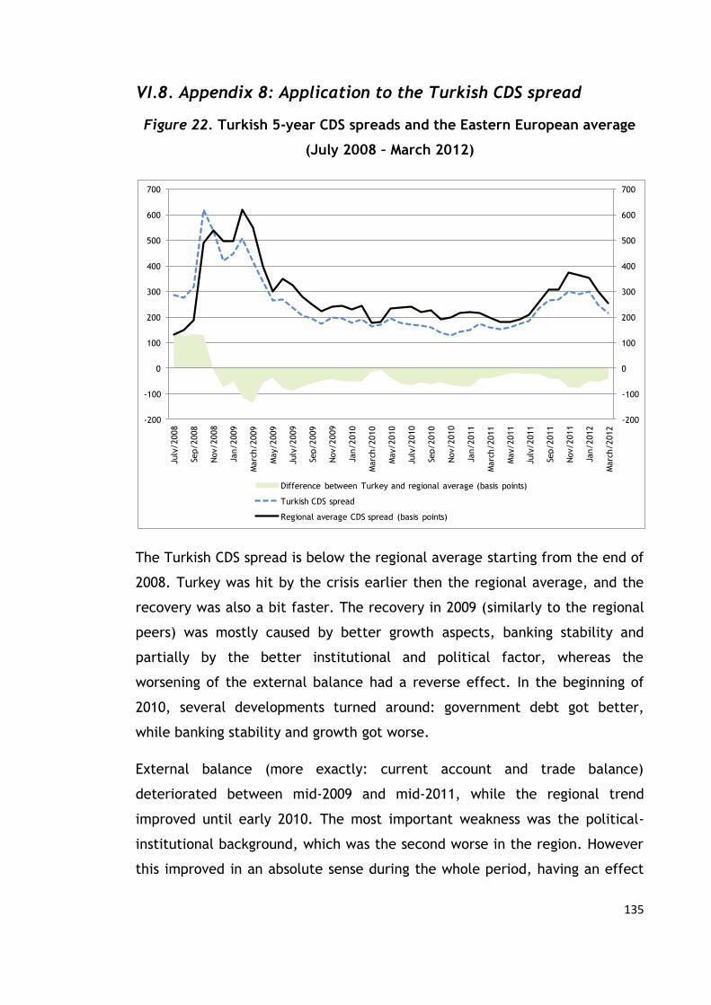
135

VI.8. Appendix 8: Application to the Turkish CDS spread

Figure 22. Turkish 5-year CDS spreads and the Eastern European average

(July 2008 – March 2012)

The Turkish CDS spread is below the regional average starting from the end of

2008. Turkey was hit by the crisis earlier then the regional average, and the

recovery was also a bit faster. The recovery in 2009 (similarly to the regional

peers) was mostly caused by better growth aspects, banking stability and

partially by the better institutional and political factor, whereas the

worsening of the external balance had a reverse effect. In the beginning of

2010, several developments turned around: government debt got better,

while banking stability and growth got worse.

External balance (more exactly: current account and trade balance)

deteriorated between mid-2009 and mid-2011, while the regional trend

improved until early 2010. The most important weakness was the political-

institutional background, which was the second worse in the region. However

this improved in an absolute sense during the whole period, having an effect

-200

-100

0

100

200

300

400

500

600

700

-200

-100

0

100

200

300

400

500

600

700

July

/2008

Sep/2008

Nov/

2008

Jan/2009

Marc

h/2009

May/

2009

July

/2009

Sep/2009

Nov/

2009

Jan/2010

Marc

h/2010

May/

2010

July

/2010

Sep/2010

Nov/

2010

Jan/2011

Marc

h/2011

May/

2011

July

/2011

Sep/2011

Nov/

2011

Jan/2012

Marc

h/2012

Difference between Turkey and regional average (basis points)

Turkish CDS spread

Regional average CDS spread (basis points)

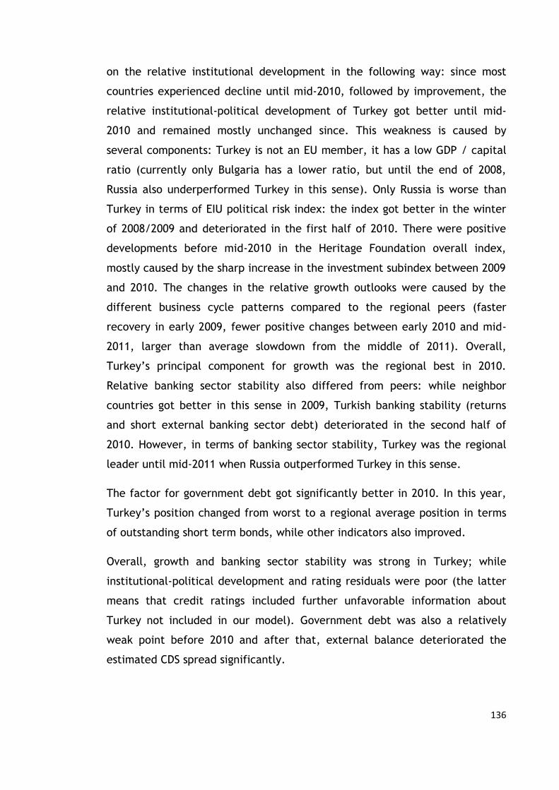
136

on the relative institutional development in the following way: since most

countries experienced decline until mid-2010, followed by improvement, the

relative institutional-political development of Turkey got better until mid-

2010 and remained mostly unchanged since. This weakness is caused by

several components: Turkey is not an EU member, it has a low GDP / capital

ratio (currently only Bulgaria has a lower ratio, but until the end of 2008,

Russia also underperformed Turkey in this sense). Only Russia is worse than

Turkey in terms of EIU political risk index: the index got better in the winter

of 2008/2009 and deteriorated in the first half of 2010. There were positive

developments before mid-2010 in the Heritage Foundation overall index,

mostly caused by the sharp increase in the investment subindex between 2009

and 2010. The changes in the relative growth outlooks were caused by the

different business cycle patterns compared to the regional peers (faster

recovery in early 2009, fewer positive changes between early 2010 and mid-

2011, larger than average slowdown from the middle of 2011). Overall,

Turkey’s principal component for growth was the regional best in 2010.

Relative banking sector stability also differed from peers: while neighbor

countries got better in this sense in 2009, Turkish banking stability (returns

and short external banking sector debt) deteriorated in the second half of

2010. However, in terms of banking sector stability, Turkey was the regional

leader until mid-2011 when Russia outperformed Turkey in this sense.

The factor for government debt got significantly better in 2010. In this year,

Turkey’s position changed from worst to a regional average position in terms

of outstanding short term bonds, while other indicators also improved.

Overall, growth and banking sector stability was strong in Turkey; while

institutional-political development and rating residuals were poor (the latter

means that credit ratings included further unfavorable information about

Turkey not included in our model). Government debt was also a relatively

weak point before 2010 and after that, external balance deteriorated the

estimated CDS spread significantly.

137

Turkey’s credit ratings were the regional worst throughout the sample;

however all three major rating agencies upgraded the country in the end of

2009.

Figure 23. Turkey: Contributions to the model-based value of the relative

CDS spread

-0.6

-0.5

-0.4

-0.3

-0.2

-0.1

0

0.1

0.2

0.3

0.4

0.5

2008.0

7.0

1

2008.0

8.0

1

2008.0

9.0

1

2008.1

0.0

1

2008.1

1.0

1

2008.1

2.0

1

2009.0

1.0

1

2009.0

2.0

1

2009.0

3.0

1

2009.0

4.0

1

2009.0

5.0

1

2009.0

6.0

1

2009.0

7.0

1

2009.0

8.0

1

2009.0

9.0

1

2009.1

0.0

1

2009.1

1.0

1

2009.1

2.0

1

2010.0

1.0

1

2010.0

2.0

1

2010.0

3.0

1

2010.0

4.0

1

2010.0

5.0

1

2010.0

6.0

1

2010.0

7.0

1

2010.0

8.0

1

2010.0

9.0

1

2010.1

0.0

1

2010.1

1.0

1

2010.1

2.0

1

2011.0

1.0

1

2011.0

2.0

1

2011.0

3.0

1

2011.0

4.0

1

2011.0

5.0

1

2011.0

6.0

1

2011.0

7.0

1

2011.0

8.0

1

2011.0

9.0

1

2011.1

0.0

1

2011.1

1.0

1

2011.1

2.0

1

2012.0

1.0

1

2012.0

2.0

1

2012.0

3.0

1

Contribution of PC_GROWTH Contribution of F_BANK Contribution of F_EXTERN

Contribution of F_GDEBT Contribution of PC_INST Contribution of FISCBAL

Contribution of RATING_RESIDS

138

Figure 24. Turkish indicators compared to regional averages

Our model’s fit is relatively good since the spring of 2009. Actual CDS was

worse than estimated before the Lehman default and in the first half of 2010;

while it outperformed the estimated values in the winter of 2008/2009 and

since mid-2011.

-2.0

-1.5

-1.0

-0.5

0.0

0.5

July

/2008

Oct

/2008

Jan/2009

Apr/

2009

July

/2009

Oct

/2009

Jan/2010

Apr/

2010

July

/2010

Oct

/2010

Jan/2011

Apr/

2011

July

/2011

Oct

/2011

Jan/2012

PC_GROWTH

PC_GROWTH

-1.8

-1.6

-1.4

-1.2

-1.0

-0.8

-0.6

-0.4

-0.2

0.0

July

/2008

Oct

/2008

Jan/2009

Apr/

2009

July

/2009

Oct

/2009

Jan/2010

Apr/

2010

July

/2010

Oct

/2010

Jan/2011

Apr/

2011

July

/2011

Oct

/2011

Jan/2012

F_BANK

F_BANK

-0.2

0.0

0.2

0.4

0.6

0.8

1.0

1.2

July

/2008

Oct

/2008

Jan/2009

Apr/

2009

July

/2009

Oct

/2009

Jan/2010

Apr/

2010

July

/2010

Oct

/2010

Jan/2011

Apr/

2011

July

/2011

Oct

/2011

Jan/2012

F_EXTERN

F_EXTERN

-0.6

-0.4

-0.2

0.0

0.2

0.4

0.6

0.8

1.0

July

/2008

Oct

/2008

Jan/2009

Apr/

2009

July

/2009

Oct

/2009

Jan/2010

Apr/

2010

July

/2010

Oct

/2010

Jan/2011

Apr/

2011

July

/2011

Oct

/2011

Jan/2012

F_GDEBT

F_GDEBT

0.0

0.5

1.0

1.5

2.0

2.5

3.0

July

/2008

Oct

/2008

Jan/2009

Apr/

2009

July

/2009

Oct

/2009

Jan/2010

Apr/

2010

July

/2010

Oct

/2010

Jan/2011

Apr/

2011

July

/2011

Oct

/2011

Jan/2012

PC_INST

PC_INST

-3.0

-2.5

-2.0

-1.5

-1.0

-0.5

0.0

0.5

1.0

1.5

2.0

July

/2008

Oct

/2008

Jan/2009

Apr/

2009

July

/2009

Oct

/2009

Jan/2010

Apr/

2010

July

/2010

Oct

/2010

Jan/2011

Apr/

2011

July

/2011

Oct

/2011

Jan/2012

FISCBAL

FISCBAL

0.0

0.5

1.0

1.5

2.0

2.5

3.0

3.5

4.0

4.5

July

/2008

Oct

/2008

Jan/2009

Apr/

2009

July

/2009

Oct

/2009

Jan/2010

Apr/

2010

July

/2010

Oct

/2010

Jan/2011

Apr/

2011

July

/2011

Oct

/2011

Jan/2012

RATINGS

RATINGS

0.0

0.5

1.0

1.5

2.0

2.5

3.0

July

/2008

Oct

/2008

Jan/2009

Apr/

2009

July

/2009

Oct

/2009

Jan/2010

Apr/

2010

July

/2010

Oct

/2010

Jan/2011

Apr/

2011

July

/2011

Oct

/2011

Jan/2012

RATING_RESIDS

RATING_RESIDS

-0.4

-0.2

0.0

0.2

0.4

0.6

0.8

1.0

1.2

July

/2008

Oct

/2008

Jan/2009

Apr/

2009

July

/2009

Oct

/2009

Jan/2010

Apr/

2010

July

/2010

Oct

/2010

Jan/2011

Apr/

2011

July

/2011

Oct

/2011

Jan/2012

log CDS spread CDSLI

log CDS spread CDSLI

139

Figure 25. The Turkish relative CDS spread and its unexplained component

The effect of the fundaments was mixed in the second half of the sample. The

estimated CDS spread improved due to the developments in government debt,

growth and institutional-political factors; while it deteriorated because of the

external and fiscal balance. Banking sector stability becoming more important

had positive, while growth aspects becoming more important and external

balance becoming less important had negative wake-up call effects.

-0.6

-0.4

-0.2

0.0

0.2

0.4

0.6

0.8

1.0

-0.6

-0.4

-0.2

0.0

0.2

0.4

0.6

0.8

1.0

July

/2008

Sep/2008

Nov/

2008

Jan/2009

Marc

h/2009

May/

2009

July

/2009

Sep/2009

Nov/

2009

Jan/2010

Marc

h/2010

May/

2010

July

/2010

Sep/2010

Nov/

2010

Jan/2011

Marc

h/2011

May/

2011

July

/2011

Sep/2011

Nov/

2011

Jan/2012

Marc

h/2012

Unexplained component Observed relative CDS spread

Model-implied relative CDS spread

140

Figure 26. Fundamental and wake-up call effects in changes of Turkish

spreads

-0.20

-0.15

-0.10

-0.05

0.00

0.05

0.10

0.15

0.20

PC

_G

RO

WT

H

F_BA

NK

F_EXT

ER

N

F_G

DEBT

PC

_IN

ST

FIS

CBA

L

RA

TIN

G_R

ESI

D

effect of fundamental change wake-up call effect

total impact on relative CDS change

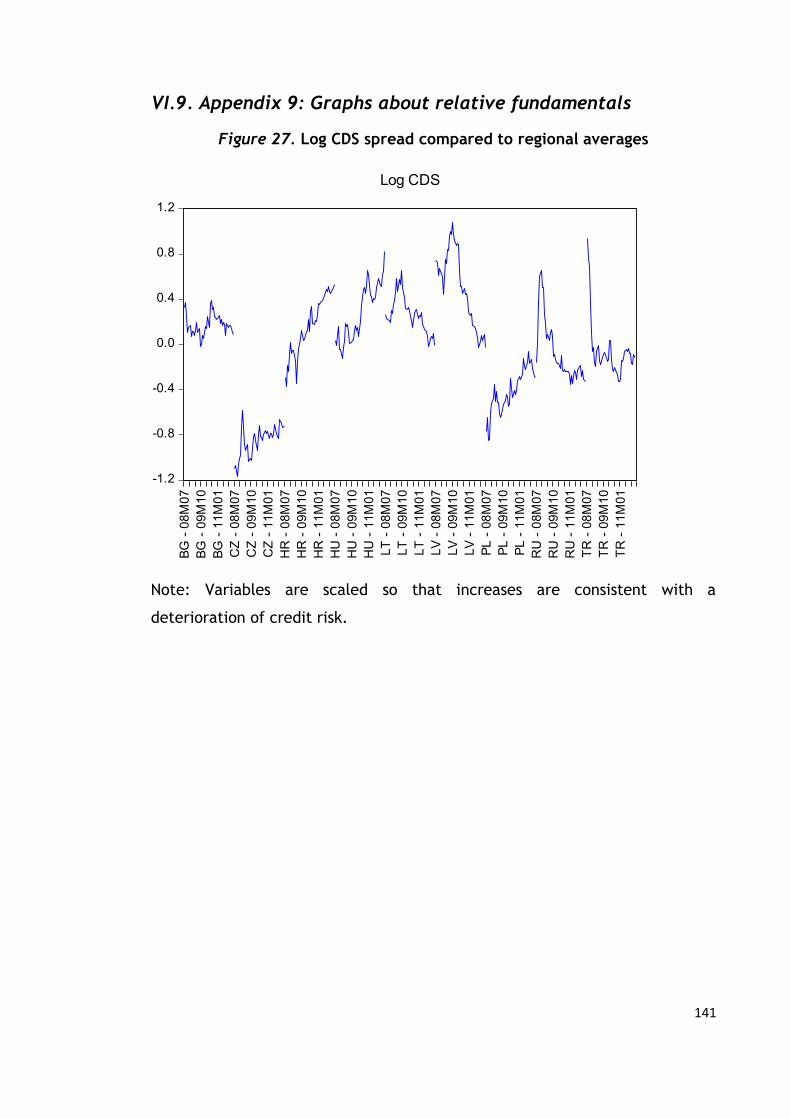
141

VI.9. Appendix 9: Graphs about relative fundamentals

Figure 27. Log CDS spread compared to regional averages

Note: Variables are scaled so that increases are consistent with a

deterioration of credit risk.

-1.2

-0.8

-0.4

0.0

0.4

0.8

1.2

BG

- 0

8M

07

BG

- 0

9M

10

BG

- 1

1M

01

CZ

- 0

8M

07

CZ

- 0

9M

10

CZ

- 1

1M

01

HR

- 0

8M

07

HR

- 0

9M

10

HR

- 1

1M

01

HU

- 0

8M

07

HU

- 0

9M

10

HU

- 1

1M

01

LT

- 0

8M

07

LT

- 0

9M

10

LT

- 1

1M

01

LV

- 0

8M

07

LV

- 0

9M

10

LV

- 1

1M

01

PL -

08M

07

PL -

09M

10

PL -

11M

01

RU

- 0

8M

07

RU

- 0

9M

10

RU

- 1

1M

01

TR

- 0

8M

07

TR

- 0

9M

10

TR

- 1

1M

01

Log CDS

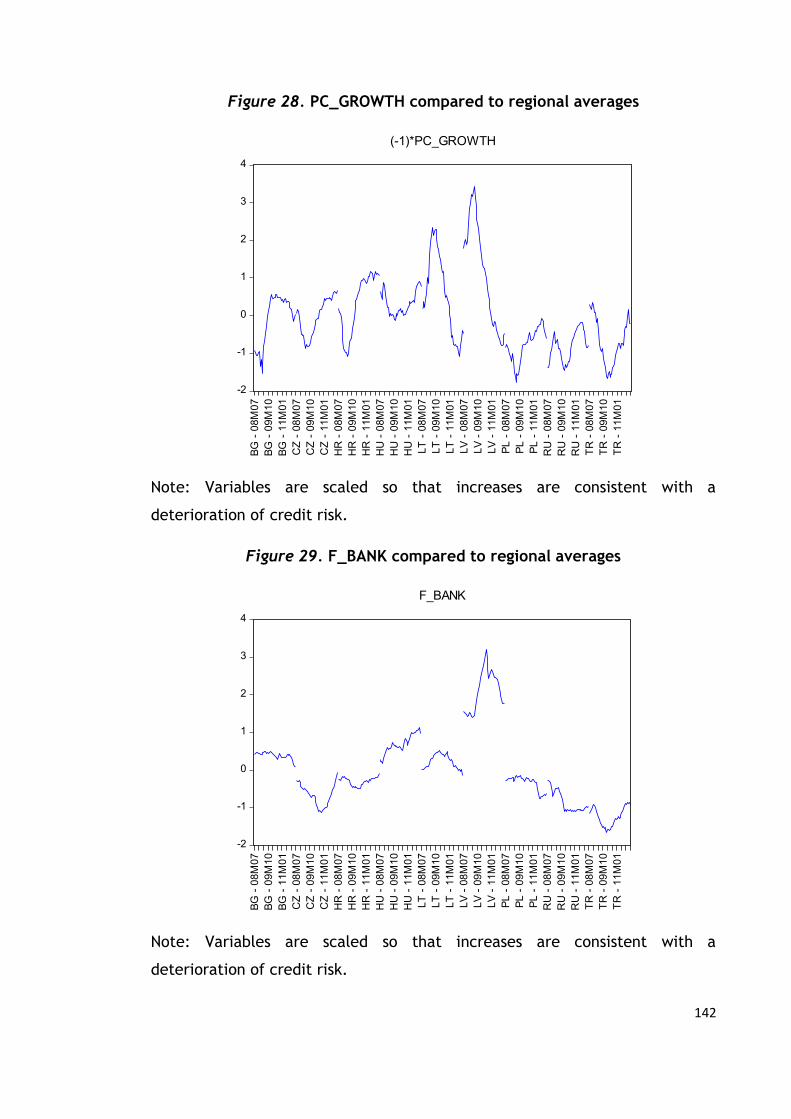
142

Figure 28. PC_GROWTH compared to regional averages

Note: Variables are scaled so that increases are consistent with a

deterioration of credit risk.

Figure 29. F_BANK compared to regional averages

Note: Variables are scaled so that increases are consistent with a

deterioration of credit risk.

-2

-1

0

1

2

3

4

BG

- 0

8M

07

BG

- 0

9M

10

BG

- 1

1M

01

CZ

- 0

8M

07

CZ

- 0

9M

10

CZ

- 1

1M

01

HR

- 0

8M

07

HR

- 0

9M

10

HR

- 1

1M

01

HU

- 0

8M

07

HU

- 0

9M

10

HU

- 1

1M

01

LT

- 0

8M

07

LT

- 0

9M

10

LT

- 1

1M

01

LV

- 0

8M

07

LV

- 0

9M

10

LV

- 1

1M

01

PL

- 0

8M

07

PL

- 0

9M

10

PL

- 1

1M

01

RU

- 0

8M

07

RU

- 0

9M

10

RU

- 1

1M

01

TR

- 0

8M

07

TR

- 0

9M

10

TR

- 1

1M

01

(-1)*PC_GROWTH

-2

-1

0

1

2

3

4

BG

- 0

8M

07

BG

- 0

9M

10

BG

- 1

1M

01

CZ

- 0

8M

07

CZ

- 0

9M

10

CZ

- 1

1M

01

HR

- 0

8M

07

HR

- 0

9M

10

HR

- 1

1M

01

HU

- 0

8M

07

HU

- 0

9M

10

HU

- 1

1M

01

LT

- 0

8M

07

LT

- 0

9M

10

LT

- 1

1M

01

LV

- 0

8M

07

LV

- 0

9M

10

LV

- 1

1M

01

PL -

08M

07

PL -

09M

10

PL -

11M

01

RU

- 0

8M

07

RU

- 0

9M

10

RU

- 1

1M

01

TR

- 0

8M

07

TR

- 0

9M

10

TR

- 1

1M

01

F_BANK

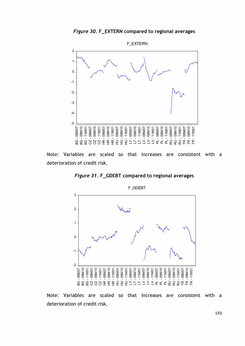
143

Figure 30. F_EXTERN compared to regional averages

Note: Variables are scaled so that increases are consistent with a

deterioration of credit risk.

Figure 31. F_GDEBT compared to regional averages

Note: Variables are scaled so that increases are consistent with a

deterioration of credit risk.

-5

-4

-3

-2

-1

0

1

2

BG

- 0

8M

07

BG

- 0

9M

10

BG

- 1

1M

01

CZ

- 0

8M

07

CZ

- 0

9M

10

CZ

- 1

1M

01

HR

- 0

8M

07

HR

- 0

9M

10

HR

- 1

1M

01

HU

- 0

8M

07

HU

- 0

9M

10

HU

- 1

1M

01

LT

- 0

8M

07

LT

- 0

9M

10

LT

- 1

1M

01

LV

- 0

8M

07

LV

- 0

9M

10

LV

- 1

1M

01

PL -

08M

07

PL -

09M

10

PL -

11M

01

RU

- 0

8M

07

RU

- 0

9M

10

RU

- 1

1M

01

TR

- 0

8M

07

TR

- 0

9M

10

TR

- 1

1M

01

F_EXTERN

-2

-1

0

1

2

3

BG

- 0

8M

07

BG

- 0

9M

10

BG

- 1

1M

01

CZ

- 0

8M

07

CZ

- 0

9M

10

CZ

- 1

1M

01

HR

- 0

8M

07

HR

- 0

9M

10

HR

- 1

1M

01

HU

- 0

8M

07

HU

- 0

9M

10

HU

- 1

1M

01

LT

- 0

8M

07

LT

- 0

9M

10

LT

- 1

1M

01

LV

- 0

8M

07

LV

- 0

9M

10

LV

- 1

1M

01

PL

- 0

8M

07

PL

- 0

9M

10

PL

- 1

1M

01

RU

- 0

8M

07

RU

- 0

9M

10

RU

- 1

1M

01

TR

- 0

8M

07

TR

- 0

9M

10

TR

- 1

1M

01

F_GDEBT

144

Figure 32. PC_INST compared to regional averages

Note: Variables are scaled so that increases are consistent with a

deterioration of credit risk.

Figure 33. FISCBAL compared to regional averages

Note: Variables are scaled so that increases are consistent with a

deterioration of credit risk.

-3

-2

-1

0

1

2

3

4

5

6

BG

- 0

8M

07

BG

- 0

9M

10

BG

- 1

1M

01

CZ

- 0

8M

07

CZ

- 0

9M

10

CZ

- 1

1M

01

HR

- 0

8M

07

HR

- 0

9M

10

HR

- 1

1M

01

HU

- 0

8M

07

HU

- 0

9M

10

HU

- 1

1M

01

LT

- 0

8M

07

LT

- 0

9M

10

LT

- 1

1M

01

LV

- 0

8M

07

LV

- 0

9M

10

LV

- 1

1M

01

PL

- 0

8M

07

PL

- 0

9M

10

PL

- 1

1M

01

RU

- 0

8M

07

RU

- 0

9M

10

RU

- 1

1M

01

TR

- 0

8M

07

TR

- 0

9M

10

TR

- 1

1M

01

(-1)*PC_INST

-6

-4

-2

0

2

4

6

BG

- 0

8M

07

BG

- 0

9M

10

BG

- 1

1M

01

CZ

- 0

8M

07

CZ

- 0

9M

10

CZ

- 1

1M

01

HR

- 0

8M

07

HR

- 0

9M

10

HR

- 1

1M

01

HU

- 0

8M

07

HU

- 0

9M

10

HU

- 1

1M

01

LT

- 0

8M

07

LT

- 0

9M

10

LT

- 1

1M

01

LV

- 0

8M

07

LV

- 0

9M

10

LV

- 1

1M

01

PL -

08M

07

PL -

09M

10

PL -

11M

01

RU

- 0

8M

07

RU

- 0

9M

10

RU

- 1

1M

01

TR

- 0

8M

07

TR

- 0

9M

10

TR

- 1

1M

01

(-1)*FISCBAL

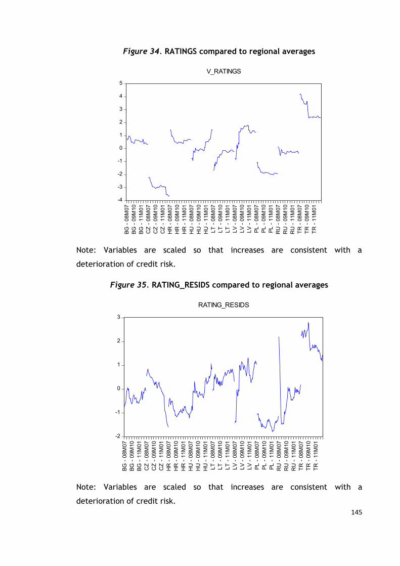
145

Figure 34. RATINGS compared to regional averages

Note: Variables are scaled so that increases are consistent with a

deterioration of credit risk.

Figure 35. RATING_RESIDS compared to regional averages

Note: Variables are scaled so that increases are consistent with a

deterioration of credit risk.

-4

-3

-2

-1

0

1

2

3

4

5

BG

- 0

8M

07

BG

- 0

9M

10

BG

- 1

1M

01

CZ

- 0

8M

07

CZ

- 0

9M

10

CZ

- 1

1M

01

HR

- 0

8M

07

HR

- 0

9M

10

HR

- 1

1M

01

HU

- 0

8M

07

HU

- 0

9M

10

HU

- 1

1M

01

LT

- 0

8M

07

LT

- 0

9M

10

LT

- 1

1M

01

LV

- 0

8M

07

LV

- 0

9M

10

LV

- 1

1M

01

PL -

08M

07

PL -

09M

10

PL -

11M

01

RU

- 0

8M

07

RU

- 0

9M

10

RU

- 1

1M

01

TR

- 0

8M

07

TR

- 0

9M

10

TR

- 1

1M

01

V_RATINGS

-2

-1

0

1

2

3

BG

- 0

8M

07

BG

- 0

9M

10

BG

- 1

1M

01

CZ

- 0

8M

07

CZ

- 0

9M

10

CZ

- 1

1M

01

HR

- 0

8M

07

HR

- 0

9M

10

HR

- 1

1M

01

HU

- 0

8M

07

HU

- 0

9M

10

HU

- 1

1M

01

LT

- 0

8M

07

LT

- 0

9M

10

LT

- 1

1M

01

LV

- 0

8M

07

LV

- 0

9M

10

LV

- 1

1M

01

PL

- 0

8M

07

PL

- 0

9M

10

PL

- 1

1M

01

RU

- 0

8M

07

RU

- 0

9M

10

RU

- 1

1M

01

TR

- 0

8M

07

TR

- 0

9M

10

TR

- 1

1M

01

RATING_RESIDS

146

VII. REFERENCES

Ábel, I. & Kóbor, Á. [2011]: Növekedés, deficit és adósság – fenntartható

keretben. Közgazdasági szemle, LVIII.(2011. június), pp.511–528.

Ades, A. et al. [2000]: Introducing GS-ESS: A New Framework for Assessing

Fair Value in Emerging Markets Hard-Currency Debt. Global Economics

Paper No. 45, Goldman Sachs, New York.

Afonso, A. [2003]: Understanding the Determinants of Sovereign Debt Ratings:

Evidence for the Two Leading Agencies. Journal of Economics and

Finance, 27(1), pp.56–74. Available at:

http://link.springer.com/10.1007/BF02751590.

DOI: http://dx.doi.org/10.1007/bf02751590

Afonso, A. & Rault, C. [2010]: Long-run Determinants of Sovereign Yields.,

CESifo Working Paper Series 3155., CESifo Group, Munich.

Aizenman, J., Hutchison, M.M. & Jinjarak, Y. [2011]: What is the Risk of

European Sovereign Debt Defaults? Fiscal Space. CDS Spreads and Market

Pricing of Risk. NBER Working Paper No.17407.

Alexopoulou, I., Bunda, I. & Ferrando, A. [2009]: Determinants of Government

Bond Spreads in the New EU Countries. ECB Working Papers No. 1093.

Allen, F. & Gale, D. [2000]: Financial Contagion. The Journal of Political

Economy, 108(1), pp.1–33. DOI: http://dx.doi.org/10.1086/262109

Alper, C.E., Forni, L. & Gerard, M. [2012]: Pricing of Sovereign Credit Risk:

Evidence from Advanced Economies During the Financial Crisis. IMF

Working Paper, WP/12/24.

Amato, J.D. [2005]: Risk Aversion and Risk Premia in the CDS Market. BIS

Quarterly Review, (December), pp.55–68.

Andenmatten, S. & Brill, F. [2011]: Measuring Co-Movements of CDS Premia

during the Greek Debt Crisis. , Discussion Paper Uni Bern No. 1104. Uni

Bern DP.

Ang, A. & Longstaff, F.A. [2011]: Systemic Sovereign Credit Risk: Lessons from

the U.S. and Europe. NBER Working Papers No. 16982.

147

Archibald, C.M., Flynn, S.T. & Malvey, P.F. [1995]: Uniform-Price Auctions  :

Evaluation of the Treasury Experience. Office of Market Finance, U.S.

Treasury Manuscript. Available at: http://www.treasury.gov/resource-

center/fin-mkts/Documents/final.pdf.

Attinasi, M.-G., Checherita, C. & Nickel, C. [2009]: What Explains the Surge in

Euro Area Sovereign Spreads During the Financial Crisis of 2007-09?.

Public Finance and Management 10, 595-645. p.

Aussenegg, W., Pichler, P. & Stomper, A. [2006]: IPO Pricing with

Bookbuilding and a When-Issued Market. The Journal of Financial and

Quantitative Analysis, 41(4), pp.829–862. Available at:

http://www.jstor.org/stable/27647276.

Ausubel, L.M. [1997]: An Efficient Ascending-Bid Auction for Multiple Objects.

University of Maryland Department of Economics Working Papers No. 97-

06. Available at: http://www.market-design.com/files/ausubel-an-

efficient-ascending-bid-auction-for-multiple-objects.pdf.

Ausubel, L.M. & Cramton, P. [2002]: Demand Reduction and Inefficiency in

Multi-Unit Auctions. University of Maryland, Department of Economics

Working Papers No. 98 wpdr. Available at:

http://drum.lib.umd.edu/bitstream/1903/7062/1/98wp-demand-

reduction.pdf.

Back, K. & Zender, J.F. [1993]: Auctions of Divisible Goods  : On the Rationale

for the Treasury Experiment. Review of Financial Studies, 6(4), pp.733–

764. DOI: http://dx.doi.org/10.1093/rfs/6.4.733

Back, K. & Zender, J.F. [2001]: Auctions of divisible goods with endogenous

supply. Economics Letters, 73(1), pp.29–34. Available at: www.nccr-

finrisk.uzh.ch/media/pdf/BackZender.pdf.

Bae, K.-H., Karolyi, G.A. & Stulz, R.M. [2000]: A New Approach to Measuring

Financial Contagion. , NBER Working Papers No. 7913.

Bai, J. & Collin-Dufresne, P. [2011]: The CDS-Bond Basis During the Financial

Crisis of 2007-2009. Available at:

http://www.ckgsb.edu.cn/Userfiles/doc/JennieBai_28Feb2012.pdf.

148

Baldacci, E., Gupta, S. & Mati, A. [2008]: Is it (Still) Mostly Fiscal?

Determinants of Sovereign Spreads in Emerging Markets. IMF Working

Paper. WP/08/259.

Balogh, C. & Kóczán, G. [2008]: Állampapírok másodpiaci kereskedési

infrastruktúrája. MNB-tanulmányok 74. Available at:

http://www.mnb.hu/Root/Dokumentumtar/MNB/Kiadvanyok/mnbhu_mn

btanulmanyok/MT_74.pdf.

Barbosa, L. & Costa, S. [2010]: Determinants of Sovereign Bond Yield Spreads

in the Euro Arae in the Context of the Economic and Financial Crisis.,

Banco de Portugal Economic Bulletin. (Autumn 2010), pp.131–150.

Bartolini, L. & Cottarelli, C. [1997]: Designing Effective Auctions for Treasury

Securities. Current Issues in Economics and Finance, Federal Reserve

Bank of New York, 3(9), pp.1–6. Available at:

http://app.ny.frb.org/research/current_issues/ci3-9.pdf.

Bauer, P. et al. [2008]: Makrogazdasági statisztikák elemzői szemmel.

Statisztikai Szemle, 86.(7-8), pp.666–694.

Beirne, J. et al. [2009]: Global and Regional Spillovers in Emerging Stock

Markets: A Multivariate GARCH-in-mean Analysis. CESifo Working Paper

Series, 2794.

Bekaert, G., Harvey, C.R. & Ng, A. [2003]: Market Integration and Contagion.

NBER Working Papers, 9510.

Benczur, P. [2001]: Identifying Sovereign Bond Risks. CEU-Economics Working

Paper, No. 9.

Benczur, P. & Ilut, C.L. [2009]: Evidence for Relational Contracts in Sovereign

Bank. Society for Economic Dynamics Meeting Papers No. 91. Available

at: http://public.econ.duke.edu/~brossi/NBERNSF/Ilut.pdf.

Benczúr, P., Simon, A. & Várpalotai, V. [2003]: Fiskális makropolitika és a

növekedés elemzése kalibrált modellel. MNB Füzetek 2003/13., Available

at:

http://english.mnb.hu/Root/Dokumentumtar/MNB/Kiadvanyok/mnbhu_m

nbfuzetek/mnbhu_mf200313/mf2003_13.pdf

Berg, S.A. et al. [2000]: Market Demand for Treasury Securities. Norges Bank

Manuscript. Available at:

149

http://wwz.unibas.ch/fileadmin/wwz/redaktion/finance/personen/yvan

/papers/logistic.pdf.

Berlinger, E., Horváth, F. & Vidovics-Dancs, Á. [2012]: Tőkeáttétel-ciklusok.

Hitelintézeti Szemle, 14(1), pp.1–23.

Berndt, A. et al. [2005]: Measuring Default Risk Premia from Default Swap

Rates and EDFs., BIS Working Papers No. 173.

Berndt, A. & Obreja, I. [2010]: Decomposing European CDS Returns. Review of

Finance, 14(March 2010), pp.189–233. Available at:

http://rof.oxfordjournals.org/cgi/doi/10.1093/rof/rfq004 [Accessed

August 29, 2013].

Bernoth, K. & Erdogan, B. [2010]: Sovereign Bond Yield Spreads: A Time-

varying Coefficient Approach. DIW Discussion Papers No. 1078., DIW,

Berlin.

Biais, B. & Faugeron-Crouzet, A.M. [2002]: IPO Auctions: English, Dutch, …

French, and Internet. Journal of Financial Intermediation, 11(1), pp.9–

36. Available at:

http://linkinghub.elsevier.com/retrieve/pii/S1042957301903195

[Accessed August 12, 2012].

Bikhchandani, S. & Huang, C. [1993]: The Economics of Treasury Securities

Markets. The Journal of Economic Perspectives, 7(3), pp.117–134.

Available at: http://www.jstor.org/stable/2138446.

Bindseil, U., Nyborg, K.G. & Strebuaev, I.A. [2002]: Bidding and Performance

in Repo Auctions: Evidence from ECB Open Market Orations. ECB Working

Papers No. 157. Available at:

http://www.ecb.int/pub/pdf/scpwps/ecbwp157.pdf.

Binmore, K. & Swierzbinski, J. [2000]: Treasury auctions: Uniform or

discriminatory? Review of Economic Design, 5(4), pp.387–410. Available

at:

http://www.springerlink.com/openurl.asp?genre=article&id=doi:10.1007/

s100580000026.

Bjonnes, G. [2001]: Bidder behavior in uniform price auctions: Evidence from

Norwegian Treasury Bond auctions. Discussion Paper September 2001.,

Norwegian Business School, Oslo.

150

Blinder, A.S. [1973]: Wage Discrimination: Reduced Form and Structural

Variables. Journal of Human Resources, 8, pp.436–455.

Bolten, S. [1973]: Treasury bill auction procedures: an empirical investigation.

The Journal of Finance, 28(3), pp.577–585. Available at:

http://onlinelibrary.wiley.com/doi/10.1111/j.1540-

6261.1982.tb03586.x/abstract [Accessed August 7, 2012].

Borgy, V. et al. [2012]: Fiscal Sustainability, Default Risk and Euro Area

Sovereign Bond Spreads. Banque de France Working Paper No. 350.

Brenner, M., Galai, D. & Sade, O. [2009]: Sovereign debt auctions: Uniform or

discriminatory? Journal of Monetary Economics, 56(2), pp.267–274.

Available at:

http://linkinghub.elsevier.com/retrieve/pii/S030439320900004X

[Accessed August 7, 2012].

Broto, C. & Pérez-Quirós, G. [2011]: Sovereign CDS Premia During the Crisis

and their Interpretation as a Measure of Risk. Banco de Espana Economic

Bulletin April, pp.134–142.

Brunnermeier, M.K. & Pedersen, L.H. [2009]: Market Liquidity and Funding

Liquidity. Review of Financial Studies, 22(6), pp.2201–2238. Available at:

http://rfs.oxfordjournals.org/cgi/doi/10.1093/rfs/hhn098 [Accessed

August 13, 2013].

Bruno, G., Ordine, M. & Scalia, A. [2005]: Banks’ participation in the

Eurosystem auctions and money market integration. Temi di discussione

No. 562. Available at:

http://www.bancaditalia.it/pubblicazioni/econo/temidi/td05/td562_05/

td562en/en_tema_562.pdf.

Cammack, E.B. [1991]: Evidence on Bidding Strategies and the Information in

Treasury Bill Auctions. Journal of Political Economy, 99(1), pp.100–130.

Available at: http://www.jstor.org/stable/2937714.

Cantor, R. & Packer, F. [1996]: Determinants and Impact of Sovereign Credit

Ratings. Federal Reserve Bank of New York Economic Policy Review,

(1996 October), pp.37–53. Available at:

http://www.iijournals.com/doi/abs/10.3905/jfi.1996.408185.

151

Chudik, A. & Fratzscher, M. [2012]: Liquidity , Risk and the Global

Transmission of the 2007-08 Financial Crises and the 2010-11 Sovereign

Debt Crisis. ECB Working Papers, 1416.

Codogno, L., Favero, C. & Missale, A. [2003]: Yield Spreads on EMU

Government Bonds. Economic Policy, 18(37), pp.503–532. Available at:

http://doi.wiley.com/10.1111/1468-0327.00114_1.

Collin-Dufresne, P., Goldstein, R.S. & Martin, J.S. [2001]: The Determinants of

Credit Spread Changes. The Journal of Finance, 56(6), pp.2177–2207.

Cox, J.C., Smith, V.L. & Walker, J.M. [1984]: Theory and Behavior of Multiple

Unit Discriminative Auctions. The Journal of Finance, 39(4), pp.983–1010.

Available at: http://www.jstor.org/stable/2327608.

Cruces, J. J. & Trebesch, C. [2013]: Sovereign Defaults: The Price of Haircuts.

American Economic Journal: Macroeconomics, 5(3), pp. 85-117.

Csonto, B. & Ivaschenko, I. [2013]: Determinants of Sovereign Bond Spreads in

Emerging Markets: Local Fundamentals and Global Factors vs. Ever-

Changing Misalignments. IMF Working Paper 13/164. Available at:

http://www.imf.org/external/pubs/ft/wp/2013/wp13164.pdf

D’Agostino, A. & Ehrmann, M. [2013]: The Pricing of G7 Sovereign Bond

Spreads: The Times, they are A-changin. MPRA Paper No. 40604.

Damianov, D.S. & Becker, J.G. [2010]: Auctions with variable supply: Uniform

price versus discriminatory. European Economic Review, 54(4), pp.571–

593. Available at:

http://linkinghub.elsevier.com/retrieve/pii/S001429210900107X

[Accessed August 12, 2012].

Damianov, D.S., Oechssler, J. & Becker, J.G. [2010]: Uniform vs.

discriminatory auctions with variable supply – experimental evidence.

Games and Economic Behavior, 68(1), pp.60–76. Available at:

http://linkinghub.elsevier.com/retrieve/pii/S0899825609001559

[Accessed August 7, 2012].

Daripa, A. [2001]: A theory of treasury auctions. Journal of International

Money and Finance, 44(0), pp.7–15. Available at:

http://www.sciencedirect.com/science/article/pii/S0261560601000225

[Accessed August 7, 2012].

152

Darvas, Z. & Wolff, G.B. [2013]: Should Non-Euro Area Countries Join the

Single Supervisory Mechanism? Danube: Law and Economics Review, 4(2),

pp.141–163. Available at:

http://www.degruyter.com/view/j/danb.2013.4.issue-2/danb-2013-

0007/danb-2013-0007.xml [Accessed August 28, 2013].

Das, S.R. & Sundaram, R.K. [1997]: Auction Theory: a Summary with

Applications to Treasury Markets. NBER Working Paper Series No. 5873.

Dasgupta, A., Leon-Gonzales, R. & Shortland, A. [2010]: Regionality Revisited:

An Examination of the Direction of Spread of Currency Crises. DIW

Discussion Papers No. 1023. DIW Berlin.

Department of the Treasury [1992]: Joint Report on the Government

Securities Market. Available at:

http://archive.org/stream/jointreportongov00unit/jointreportongov00uni

t_djvu.txt.

Dovern, J., Fritsche, U. & Slacalek, J. [2012]: Disagreement among

Forecasters in G7 Countries. The Review of Economics and Statistics,

94(4), pp.1081–1096. Available at:

http://www.mitpressjournals.org/doi/pdf/10.1162/REST_a_00207.

Duffie, D., Pedersen, L.H. & Singleton, K.J. [2003]: Modeling Sovereign Yield

Spreads: A Case Study of Russian Debt. The Journal of Finance, LVIII(1),

pp.119–160.

Dungey, M. et al. [2003]: Characterizing Global Investors’ Risk Appetite for

Emerging Market Debt During Financial Crises. , IMF Working Papers No.

03/251.

Dungey, M. & Martin, V.L. [2007]: Unravelling Financial Market Linkages

During Crises. Journal of Applied Econometrics, 22(1), pp.89–119.

Eaton, J. & Gersovitz, M. [1981]: Debt with Potential Repudiation: Theoretical

and Empirical Analysis. Review of Economic Studies, 48, 289-309.

Ebner, A. [2009]: An Empirical Analysis on the Determinants of CEE

Government Bond Spreads. Emerging Markets Review, 10(2), pp.97–121.

Available at:

http://linkinghub.elsevier.com/retrieve/pii/S1566014109000119

[Accessed August 28, 2013].

153

Edwards, S. [1983]: LDC’s Foreign Borrowing and Default Risk: An Empirical

Investigation 1976-1980. American Economic Review, vol. 74 (4)

September, AEA, 726–734. p.

Edwards, S. [1985]: The Pricing of Bonds and Bank Loans in International

Markets: An Empirical Analysis of Developing Countries’ Foreign

Borrowing. European Economic Review. Volume 30, Issue 3, June 1986,

565–589. p.

Eichengreen, B. & Mody, A. [1998]: What Explains Changing Spreads on

Emerging-Market Debt: Fundamentals or Market Sentiment? NBER Working

Papers No. 6408. NBER.

Ejsing, J.W. & Lemke, W. [2009]: The Janus-Headed Salvation Sovereign and

Bank Credit Risk Premia During 2008-09. ECB Working Papers No. 1127.,

ECB.

Elsinger, H., Schmidt-Dengler, P. & Zulehner, C. [2012]: Competition in

Austrian Treasury Auctions. Oesterreichische Nationalbank Working

Papers Forthcoming. Available at:

http://www.wcas.northwestern.edu/csio/Conferences/SchmidtDenglerPa

per.pdf.

Elsinger, H., Zulehner, C. & Schmidt-Dengler, P. [2007]: Bidding Behaviour in

Austrian Treasury Bond Auctions. Monetary Policy and the Economy, (2

(August 2007)), pp.109–125. Available at:

http://ideas.repec.org/a/onb/oenbmp/y2007i2b6.html.

Engelbrecht-Wiggans, R. & Kahn, C.M. [1998]: Economic Theory. Economic

Theory, 12(2), pp.227–258. Available at:

http://www.jstor.org/stable/25055122.

Engelmann, D. & Grimm, V. [2009]: Bidding Behavior in Multi – Unit Auctions —

An Experimental Investigation. The Economic Journal, 119(537), pp.855–

882. Available at: http://onlinelibrary.wiley.com/doi/10.1111/j.1468-

0297.2009.02249.x/abstract.

Erb, C.B., Harvey, C.R. & Viskanta, T.E. [1996]: Political Risk, Economic Risk

and Financial Risk. Financial Analysts Journal, 52(6), pp.29–46. Available

at: http://www.cfapubs.org/doi/abs/10.2469/faj.v52.n6.2038.

Erhart, S. et al. [2013]: Mindenki másképp csinálja avagy A jegybankmérlegek

és a jegybanki eszköztár átalakulása néhány feltörekvő országban. MNB

154

Szemle, 2013. Október. Különszám, pp.48–62.

http://www.mnb.hu/Root/Dokumentumtar/MNB/Kiadvanyok/mnbhu_mn

bszemle/mnbhu_msz_20131030/erhart.pdf

Eső, P. [1997]: Árverés és verseny a közbeszerzésben. Közgazdasági szemle,

XLIV.(July - August), pp.597–611. Available at:

http://epa.oszk.hu/00000/00017/00029/pdf/eso.pdf.

Fabra, N. [2003]: Tacit Collusion in Repeated Auctions : Uniform versus

Discriminatory. The Journal of Industrial Economics, 51(3), pp.271–293.

Available at: http://www.jstor.org/stable/3569711.

Favero, C., Pagano, M. & von Thadden, E.-L. [2010]: How Does Liquidity

Affect Government Bond Yields? Journal of Financial and Quantitative

Analysis, 45(01), pp.107–134.

Feldman, R.A. & Reinhart, V. [1995]: Auction Format Matters: Evidence on

Bidding Behavior and Selling Revenue. IMF Working Paper No. 95/47.

Available at:

http://adlib.imf.org/digital_assets/wwwopac.ashx?command=getcontent

&server=webdocs&value=EB/1995/WP/13935.PDF.

Ferrucci, G. [2003]: Empirical Determinants of Emerging Market Economies’

Sovereign Bond Spreads. BoE Working Papers No. 205., BoE.

Février, P., Raphaele, P. & Visser, M. [2004]: Econometrics of Share Auctions.

Department of Economics, University of Chicago Manuscript. Available at:

http://www.econ.yale.edu/seminars/apmicro/am04/fevrier-040401.pdf.

Forbes, K.J. & Chinn, M.D. [2003]: A Decomposition of Global Linkages in

Financial Markets Over Time. , pp.1–51.

Forbes, K.J. & Rigobon, R. [2002]: No Contagion, Only Interdependence:

Measuring Stock Market Comovements. Journal of Finance, LVII(5),

pp.2223–2261.

Friedman, M. [1991]: How to Sell Government Securities Wall Street Journal,

28 August 1991. Wall Street Journal, (August), p.A8. Available at:

http://0055d26.netsolhost.com/friedman/pdfs/wsj/WSJ.08.28.1991.pdf.

Friedman, M. [1959]: Testimony in Employment, Growth, and Price Levels.

Joint Economic Committee, 86th Congress, 1st Session, October 30.

Available at: http://papers.nber.org/books/fabr61-1

155

Gai, P. & Vause, N. [2006]: Measuring Investors’ Risk Appetite. International

Journal of Central Banking, 1, pp.167–188.

Gapen, M.T. et al. [2005]: Measuring and Analyzing Sovereign Risk with

Contingent Claims. IMF Staff Papers, 55(1), pp.1–49. Available at:

http://www.palgrave-

journals.com/doifinder/10.1057/palgrave.imfsp.9450026.

Goldfajn, I. & Valdes, R.O. [1997]: Capital Flows and the Twin Crises: The

Role of Liquidity. IMF Working Papers, 97/87. IMF.

Gordy, M.B. [1999]: Hedging Winer’s Curse with Multiple Bids: Evidence from

the Portuguese Treasury Bill Auction. The Review of Economics and

Statistics, 81(3), pp.448–465. Available at:

http://www.jstor.org/stable/2646768.

Goswami, G., Noe, T.H. & Rebello, M.J. [1996]: Collusion in Uniform-Price

Auctions : Experimental Evidence and Implications for Treasury Auctions.

The Review of Financial Studies, 9(3), pp.757–785. Available at:

http://www.jstor.org/stable/2962310.

Hamao, Y. & Jegadeesh, N. [1998]: An Analysis of Blidding in the Japanese

Government Bond Auctions. The Journal of Finance, 53(2), pp.755–772.

Available at: http://www.jstor.org/stable/117369.

Harris, M. & Raviv, A. [1981]: Allocation Mechanisms and the Design of

Auctions. Econometrica, 49(6), pp.1477–1499. Available at:

http://www.jstor.org/stable/1911413.

Haugh, D., Ollivaud, P. & Turner, D. [2009]: What Drives Sovereign Risk

Premiums?: An Analaysis of Recent Evidence from the Euro Area. OECD

Economics Department Working Papers, No. 718., OECD.

Heller, D. & Lengwiler, Y. [2001]: Should the Treasury Price-Discriminate ? A

Procedure for Computing Hypothetical Bid Functions. Journal of

Institutional and Theoretical Economics, 157, pp.413–429. Available at:

http://wwz.unibas.ch/fileadmin/wwz/redaktion/finance/personen/yvan

/papers/heller-lengwiler-01.pdf.

Hilscher, J. & Nosbusch, Y. [2010]: Determinants of Sovereign Risk:

Macroeconomic Fundamentals and the Pricing of Sovereign Debt. Review

of Finance, 14(2), pp.235–262. Available at:

156

http://rof.oxfordjournals.org/cgi/doi/10.1093/rof/rfq005 [Accessed

August 19, 2013].

Horatcsu, A. [2002]: Bidding Behavior in Divisible Good Auctions : Theory and

Evidence from the Turkish Treasury Auction Market. Available at:

http://home.uchicago.edu/~hortacsu/paper2_aug2.pdf.

Horatcsu, A. - McAdams, D. [2010]: Mechanism Choice and Strategic Bidding in

Divisible Good Auctions: An Empirical Analysis of the Turkish Treasury

Auction Market. Journal of Political Economy, 2010, 118(5), pp. 833-865.

http://www.jstor.org/stable/10.1086/657948

Hudson, R. [2000]: Analysis of uniform and discriminatory price auctions in

restructured electricity markets. Relatório Técnico, Oak Ridge National

Laboratory, Oak …, pp.1–7. Available at:

http://www.ornl.gov/sci/ees/etsd/pes/pubs/pricing.pdf [Accessed

August 7, 2012].

Kaminska, I. [2010]: A loser’s nightmare in Europe’s debt auctions? Financial

Times Alphaville. Available at:

http://ftalphaville.ft.com/blog/2010/09/24/351991/a-losers-nightmare-

in-europes-debt-auctions/.

Kandel, S., Sarig, O. & Wohl, A. [1999]: The demand for stocks: an analysis of

IPO auctions. Review of Financial Studies, 12(2), pp.227–247. Available

at: ftp://www1.idc.ac.il/Faculty/sarig/sarigo/demand.pdf.

Kang, B. & Puller, S.L. [2008]: The Effect of Auction Format on Efficiency and

Revenue in Divisible Goods Auctions: a Test. The Journal of Industrial

Economics, LVI(2), pp.290–332. Available at:

http://citeseerx.ist.psu.edu/viewdoc/summary?doi=10.1.1.75.5985.

Keloharju, M., Nyborg, K.G. & Rydqvist, K. [2005]: Treasury Auctions Strategic

Behavior and Underpricing in Uniform Price Auctions : Evidence from

Finnish Treasury Auctions. The Journal of Finance, 60(4), pp.1865–1902.

Available at: http://www.jstor.org/stable/pdfplus/3694856.pdf.

Kim, D.H., Loretan, M. & Remolona, E.M. [2009]: Contagion and Risk Premia in

the Amplification of Crisis: Evidence from Asian Names in the Global CDS

Market. Journal of Asian Economics, 21(3), pp.314–326. Available at:

http://linkinghub.elsevier.com/retrieve/pii/S1049007809000669

[Accessed August 28, 2013].

157

Király, J. et al. [2008]: Retail Credit Expansion and External Finance in

Hungary: Lessons from the Recent Past (1998 – 2007). BIS Papers

chapters, Financial globalisation and emerging market capital flows,

(44), pp.221–233.

Kisgergely, K. [2009]: What Moved Sovereign CDS Spreads in the Period of

Financial Turbulence? Report on Financial Stability, MNB, November

2009.

Klemperer, P. [2004]: Auctions: Theory and Practice. Princetone: Princeton

University Press. Available at:

http://www.nuff.ox.ac.uk/users/klemperer/VirtualBook/VirtualBookCov

erSheet.asp.

Klemperer, P. [2002]: What Really Matters in Auction Design. The Journal of

Economic Perspectives, 16(1), pp.169–189. Available at:

http://www.jstor.org/stable/2696581.

Kocsis, Z. - Monostori, Z. [2013a]: Country-Specific Determinants of Sovereign

CDS Spreads: the Role of Fundamentals in Eastern Europe. Magyar

Közgazdaságtudományi Egyesület (MKE) konferencia. Budapest.

Kocsis, Z. - Monostori, Z. [2013b]: Country-Specific Determinants of Sovereign

CDS Spreads: the Role of Fundamentals in Eastern Europe. In Annual

Financial Market Liquidity Conference. Budapest.

Kocsis, Z. & Mosolygó, Z. [2006]: A devizakötvény-felárak és a

hitelminõsítések összefüggése – keresztmetszeti elemzés. Közgazdasági

szemle, LIII(2006. szeptember), pp.769–798.

Kocsis, Z. & Nagy, D. [2011]: Variance Decomposition of Sovereign CDS

Spreads. MNB Bulletin, (October 2011), pp.36–50.

Kodres, L.E. & Pritsker, M. [2002]: A Rational Expectations Model of Financial

Contagion. The Journal of Finance, LVII(2), pp.769–799.

Koesrindartoto, D. [2004]: Treasury Auction, Uniform or Discriminatory?: An

Agent-Based Approach. Iowa State Uniiversity, Department of Economics

Working Paper No. 04013. Available at:

http://www2.econ.iastate.edu/research/webpapers/paper_11988_04013

.pdf [Accessed August 7, 2012].

158

Kondrát, Z. [1996]: Az aukcios modszer hatása a kincstár bevételére.

Közgazdasági szemle, XLIII. (Ju, pp.506–524. Available at:

http://epa.oszk.hu/00000/00017/00017/pdf/kondrat.pdf

Kremer, Ilan & Nyborg, K.G. [2004]: Divisible-good auctions: the role of

allocation rules. The RAND Journal of Economics, 35(1), pp.147–159.

Available at: http://www.jstor.org/stable/1593734.

Kremer, Ilian & Nyborg, K.G. [2004]: Underpricing and market power in

uniform price auctions. Review of Financial Studies, 17(3), pp. 849-877.

Available at: http://rfs.oxfordjournals.org/content/17/3/849.short

[Accessed August 7, 2012].

Krishna, V. [2009]: Auction theory Second ed. San Diego: Academic Press.

Available at:

http://books.google.com/books?hl=en&lr=&id=qW1128ktG1gC&oi=fnd&pg

=PP1&dq=Auction+Theory&ots=SS4i8Q6MIj&sig=f984hoRGpa41qGLKfPd90H

edolw [Accessed August 7, 2012].

LiCalzi, M. & Pavan, A. [2005]: Tilting the supply schedule to enhance

competition in uniform-price auctions. European Economic Review, 49(1),

pp.227–250. Available at:

http://linkinghub.elsevier.com/retrieve/pii/S0014292102003240

[Accessed August 7, 2012].

Linzert, T., Nautz, D. & Breitung, J. [2006]: Bidder behavior in central bank

repo auctions: Evidence from the Bundesbank. Journal of International

Financial Markets, Institutions and Money, 16(3), pp.215–230. Available

at: http://ac.els-cdn.com/S1042443105000478/1-s2.0-

S1042443105000478-main.pdf?_tid=43a5e2c6-1dbc-11e2-b678-

00000aacb35d&acdnat=1351070700_6e7e2967497292366fd06d0d9ae0c96e

[Accessed October 25, 2012].

List, J.A. & Lucking-Reiley, D. [2000]: Demand reduction in multiunit

auctions: Evidence from a sportscard field experiment. The American

Economic Review, 90(4), pp.961–972. Available at:

http://www.jstor.org/stable/10.2307/117317 [Accessed August 7, 2012].

Longstaff, F.A. et al. [2011]: How Sovereign is Sovereign Credit Risk? American

Economic Journal: Macroeconomics, 3(2), pp.75–103. Available at:

http://www.nber.org/papers/w13658.pdf.

159

Maltritz, D. & Molchanov, A. [2013]: Country Credit Risk Determinants with

Model Uncertainty. International Review of Economics and Finance,

Accepted Manuscript. Available at:

http://linkinghub.elsevier.com/retrieve/pii/S1059056013000531

[Accessed August 29, 2013].

Manganelli, S. & Wolswijk, G. [2009]: What Drives Spreads in the Euro Area

Government Bond Market? Economic Policy, 24(58), pp.191–240.

Marszalec, D. [2008]: A Structural Econometric Analysis of Polish Treasury Bill

Auctions. Department of Economics and Nuffield College, University of

Oxford Manuscript. Available at:

http://www.webmeets.com/files/papers/EARIE/2009/214/DMarszalec_T

BillAuctions_Feb09.pdf.

Maxwell, C.C. [1983]: Auctioning divisible commodities: A study of price

determination. Doctoral Dissertation. Harward University.

McAdams, D. [2007]: Adjustable supply in uniform price auctions: Non-

commitment as a strategic tool. Economics Letters, 95(1), pp.48–53.

Available at:

http://linkinghub.elsevier.com/retrieve/pii/S0165176506003156

[Accessed August 12, 2012].

Mccabe, K.A., Rassenti, S.J. & Smith, V.L. [1990]: Auction Institutional

Design : Theory and Behavior of Simultaneous Multiple-Unit

Generalizations of the Dutch and English Auctions. The American

Economic Review,, 80(5), p.The American Economic Review. Available at:

http://www.jstor.org/stable/2006779.

Mcguire, P. & Schrijvers, M.A. [2003]: Common Factors in Emerging Market

Spreads. BIS Quarterly Review, (December 2003), pp.65–78.

Merton, R.C. [1974]: On the Pricing of Corporate Debt: The Risk Structure of

Interest Rates. Journal of Finance, 29(2), pp.449–470.

Mester, L.J. [1995]: There’s more than one way to sell a security: The

Treasury’s Auction Experiment. Federal Reserve Bank of Philadelphia

Business Review. Available at: http://www.philadelphiafed.org/research-

and-data/publications/business-review/1995/brja95lm.pdf.

160

Milgrom, P.R. & Weber, R.J. [1982]: A Theory of Auctions and Competitive

Bidding. Econometrica, 50(5), pp.1089–1122. Available at:

http://www.jstor.org/stable/1911865.

Miller, M. [1991]: Interview with Merton Miller. The New York Times, 15th

September, p.3:13. Available at:

http://www.nytimes.com/1991/09/15/business/wall-street-diana-b-

henriques-treasury-s-troubled-auctions.html.

Min, H.G. [1999]: Determinants of Emerging Market Bond Spread: Do Economic

Fundamentals Matter? Policy Research Working Paper No. WPS 1899, The

World Bank, Washington D.C.

Mody, A. [2009]: From Bear Stearns to Anglo Irish: How Eurozone Sovereign

Spreads Related to Financial Sector Vulnerability. IMF Working Paper, No.

108.

Monostori, Z. [2014]: Discriminatory versus Uniform-price Auctions. MNB

Occasional Papers No. 111.

http://www.mnb.hu/Root/Dokumentumtar/MNB/Kiadvanyok/mnbhu_mn

btanulmanyok/OP111_final.pdf.

Monostori, Z. [2013a]: Diszkriminatív áras és egyenáras aukciók I. rész:

elméleti eredmények. In Doctoral Student Conference. Budapesti

Corvinus Egyetem.

Monostori, Z. [2013b]: Diszkriminatív áras és egyenáras aukciók II. rész:

empirikus eredmények. In Doctoral Student Conference. Budapesti

Corvinus Egyetem.

Monostori, Z. [2013c]: Diszkriminatív áras és egyenáras aukciók. Közgazdasági

Szemle, LX., pp. 1048-1074..

http://www.kszemle.hu/tartalom/letoltes.php?id=1415

Monostori, Z. [2013d]: Why did the Polish treasury change the auction format?

In Workshop on Impact of global crisis on EU and CEECs governance and

financial markets. Corvinus University of Budapest.

Monostori, Z. [2013e]: Crisis on the Hungarian Government Bond Markets in

the Winter of 2011-2012: Was that a Liquidity Problem? Society and

Economy. 35 (4), pp. 539-550.

DOI: http://dx.doi.org/10.1556/socec.2013.0009

161

Monostori, Z. [2012a]: Szuverén forintkötvények hozamainak dekompozíciója.

In Vállalkozói- és Gazdasági Trendek a Kárpát-medencében Konferencia.

Miercurea Ciuc.

Monostori, Z. [2012b]: Magyar szuverén fix kamatozású forintkötvények

hozamdekompozíciója. Hitelintézeti Szemle, 11(5), pp.462–475.

http://www.bankszovetseg.hu/wp-content/uploads/2012/10/462-475-

monostori.pdf

Monostori, Z. [2012c]: Crisis on the Hungarian Government Bond Markets: Is

that a Liquidity Problem? In 7th South East European Doctoral Student

Conference. Thessaloniki.

Monostori, Z. [2012d]: Is there a Liquidity Problem on the Hungarian Sovereign

Bond Makets? In Spring Wind Conference. Győr.

Monostori, Z. [2011a]: Az ötéves magyar szuverén fix kamatozású

forintkötvények hozamainak dekompozíciója. In OTDK dolgozat. Gödöllő.

Monostori, Z. [2011b]: Liquidity of Hungarian sovereign bond markets during

the crisis. In Annual Financial Market Liquidity Conference. Budapest.

Monostori, Z. [2010]: Az ötéves, magyar, szuverén, fix kamatozású

forintkötvények hozamainak dekompozíciója. In TDK dolgozat. Budapesti

Corvinus Egyetem.

Morgan Stanley [2012]: Emerging Markets - Local Markets Guidebook.

Available at: http://www.docstoc.com/docs/118900740/Morgan-Stanley-

--Local-Markets-Guidebook.

Nautz, D. [1995]: Zur Fernsteuerung des Geldmarktes durch die

Wertpapierpenisongeschäfte der Bundesbank. Zeitschrift für Wirtschafts-

und Sozialwissenschaten, 115(4), pp.623–644.

Nickel, C., Rother, P.C. & Rülke, J.C. [2009]: Fiscal Variables and Bond

Spreads – Evidence from Eastern European Countries. ECB Working

Papers, 1101. ECB.

Noussair, C. [1994]: Equilibria in a multi-object uniform price sealed bid

auction with multi-unit demands. Economic Theory, 5, pp.337–351. DOI:

http://dx.doi.org/10.1007/bf01215207

162

Nyborg, K.B. & Strebulaev, I.A. [2004]: Multiple unit auctions and short

squeezes. Review of Financial Studies, 17(2), pp.545–580. DOI:

http://dx.doi.org/10.1093/rfs/hhg038

Nyborg, K.G., Rydqvist, K. & Sundaresan, S.M. [2002]: Bidder Behavior in

Multi-Unit Auctions - Evidence from Swedish Treasury Auctions. Journal of

Political Economy, 110(2), pp.394–424. Available at:

http://www0.gsb.columbia.edu/faculty/ssundaresan/PDFpapers/bidding

_multiunit_auctions.pdf.

Nyborg, K.G. & Sundaresan, S. [1996]: Discriminatory versus uniform Treasury

auctions : Evidence from when-issued transactions. Journal of Financial

Economics, 42, pp.63–104. DOI: http://dx.doi.org/10.1016/0304-

405x(95)00871-b

Oaxaca, R. [1973]: Male-Female Wage Differentials in Urban Labor Markets.

International Economic Review, 14(October), pp.693–709.

Páles, J. & Homolya, D. [2011]: A hazai bankrendszer külföldi

forrásköltségeinek alakulása. MNB-szemle, (2011 október), pp.61–69.

Pan, J. & Singleton, K.J. [2008]: Default and Recovery Implicit in the Term

Structure of Sovereign CDS Spreads. The Journal of Finance, LXIII(5),

pp.2345–2384.

Panizza, U., Sturzenegger, F. & Zettelmeyer, J. [2009]: The Economics and

Law of Sovereign Debt and Default. Journal of Economic Literature,

47(3), pp.653–700. DOI: http://dx.doi.org/10.1257/jel.47.3.651

Pericoli, M. & Sbracia, M. [2001]: A Primer on Financial Contagion. Journal of

Economic Surveys, vol. 17, pp. 571-608.

Puhle, M. [2008]: Bond Portfolio Optimization. Verlag Berlin Heidelberg:

Springer.

Reinhart, C.M. & Kaminsky, G.L. [2000]: On Crises, Contagion and Confusion.

Journal of International Economics, 51(1), pp.145–168.

Remolona, E.M., Scatigna, M. & Wu, E. [2008]: A Ratings Based Approach to

Measuring Expected Losses from Sovereign Defaults. International Journal

of Finance & Economics, 13(1), pp.26–39.

163

Van Rijckeghem, C. & Weder, B. [2001]: Sources of contagion: is it finance or

trade? Journal of International Economics, 54(2), pp.293–308. DOI:

http://dx.doi.org/10.1016/s0022-1996(00)00095-7

Rocholl, J. [2005]: Discriminatory auctions with seller discretion : evidence

from German treasury auctions. Deutsche Bundesbank. Discussion Paper

Series, (15). Available at:

http://www.bundesbank.de/Redaktion/EN/Downloads/Publications/Disc

ussion_Paper_1/2005/2005_05_06_dkp_15.pdf? blob=publicationFile.

Rowland, P. [2004]: Determinants of Spread , Credit Ratings and

Creditworthiness for Emerging Market Sovereign Debt: A Follow-Up Study

Using Pooled Data Analysis. Borradores de Economia Nu. 296, Banco de la

Republica de Colombia.

Sade, O., Schnitzlein, C. & Zender, J.F. [2006]: Competition and Cooperation

in Divisible Good Auctions: An Experimental Examination. Review of

Financial Studies, 19(1), pp.195–235. Available at: http://leeds-

faculty.colorado.edu/zender/papers/SSZ1.pdf [Accessed August 12,

2012].

De Santis, R.A. [2012]: The Euro Area Sovereign Debt Crisis: Safe Haven,

Credit Rating and the Spread of the Fever from Greece, Ireland and

Porugal. ECB Working Papers, No. 1419. ECB.

Sareen, S. [2004]: Cross-Country Comparison of Models for Issuance of

Government Securities. Duke University Department of Economics

Manuscript. Available at:

http://www.geocities.ws/samitasareen/ctry_summ_boc_mod0603.pdf.

Scalia, A. [1997]: Bidder Profitability under Uniform Price Auctions and

Systematic Reopenings: the Case of Italian Treasury Bonds. Bank of Italy

Working Paper No. 303. Available at:

http://papers.ssrn.com/sol3/papers.cfm?abstract_id=1804020.

Schuknecht, L., von Hagen, J. & Wolswijk, G. [2010]: Government Bond Risk

Premiums in the EU Revisited - The Impact of the Financial Crisis. ECB

Working Papers, 1152. ECB.

Sgherri, S. & Zoli, E. [2009]: Euro Area Sovereign Risk During the Crisis. IMF

Working Papers, WP/09/222. IMF.

164

Simon, D.P. [1994]: The Treasury’s Experiment with Single-Price Auctions in

the Mid-1970s: Winner's or Taxpayer's Curse? The Review of Economics

and Statistics, 76(4), pp.754–760. Available at:

http://www.jstor.org/stable/pdfplus/2109776.pdf.

Smith, V.L. [1967]: Experimental Studies of Discrimination Versus Competition

in Sealed-Bid Auction Markets. The Journal of Business, 40(1), pp.56–84.

Available at: http://www.jstor.org/stable/2351305.

Sturzenegger, F. & Zettelmeyer, J. [2005]: Haircuts: Estimating Investor

Losses in Sovereign Debt Restructurings, 1998–2005. Journal of

International Money and Finance, 27(5), pp.1–67. DOI:

http://dx.doi.org/10.1016/j.jimonfin.2007.04.014

Sundaresan, S. [1994]: An Empirical Analysis of U.S. Treasury Auctions

Implications for Auction and Term Structure Theories. The Journal of

Fixed Income, 4(2), pp.35–50. Available at:

http://www.iijournals.com/doi/abs/10.3905/jfi.1994.408109.

Szatmári, A. [1996a]: Aukciók, avagy a képbe kerül, ha a Louvre a képbe

kerül? Közgazdasági szemle, XLIII.(April), pp.303–314.

Szatmári, A. [1996b]: DKJ. In TDK dolgozat. Budapesti Corvinus Egyetem.

Szűcs, N., Havran, D. & Csóka, P. [2010]: Információs paradoxon a

vállalkozások hitelezésében nem fizető vevő esetén. Közgazdasági

szemle, LVII(2010 április), pp.318–336.

Tenorio, R. [1993]: Revenue Equivalence and Bidding Behavior in a Multi-Unit

Auction Market: An Empirical Analysis. The Review of Economics and

Statistics, 75(2), pp.302–314. Available at:

http://www.jstor.org/stable/2109436.

Tsao, C.S. & Vignola, A.J. [1977]: Price Discrimination and the Demand for

Treasury’s Long Term Securities. U.S. Department of Treasury

Manuscript.

Umlauf, S.R. [1993]: An empirical study of the Mexican Treasury bill auction.

Journal of Financial Economics, 33(3), pp.313–340. Available at:

http://www.sciencedirect.com/science/article/pii/0304405X93900109.

Varga, L. [2009]: The Information Content of Hungarian Sovereign CDS

Spreads. MNB Occassional Papers No. 78.. Available at:

165

http://english.mnb.hu/Root/Dokumentumtar/ENMNB/Kiadvanyok/mnben

_muhelytanulmanyok/mnben_op_78/op_78.pdf

Vasicek, B. & Claeys, P. [2012]: Measuring Sovereign Bond Spillover in

Europeand the Impact of Rating News. ECB Working Paper, forthcoming.

ECB.. Available at:

http://www.cnb.cz/miranda2/export/sites/www.cnb.cz/en/research/re

search_publications/cnb_wp/download/cnbwp_2012_07.pdf.

Vickrey, W. [1961]: Counterspeculation, Auctions, and Competitive Sealed

Tenders. The Journal of Finance, 16(1), pp.8–37. Available at:

http://www.jstor.org/stable/2977633.

Viswanathan, S. & Wang, J.J.D. [2000]: Auctions with when-issued trading: a

model of the US Treasury markets. Manuscript, 2. Available at:

http://scholar.google.com/scholar?hl=en&btnG=Search&q=intitle:Auction

s+with+When-Issued+Trading:+a+Model+of+the+U.S.+Treasury+Markets#0

[Accessed August 7, 2012].

Wang, J.J.D. & Zender, J.F. [2002]: Auctioning divisible goods. Economic

Theory, 19(4), pp.673–705. DOI:

http://dx.doi.org/10.1007/s001990100191

Wang, M.-C. & Shih, F.-M. [2010]: Volatility Spillover: Dynamic Regional and

World Effects. European Journal of Scientific Research, 41(4), pp.582–

589.

Weigel, D. & Gemmill, G. [2006]: What Drives Credit Risk in Emerging

Markets? The Roles of Country Fundamentals and Market Co-movements.

Journal of International Money and Finance, 25(3), pp.476–502. DOI:

http://dx.doi.org/10.1016/j.jimonfin.2006.01.006

Wilson, R. [1979]: Auctions of Shares Author. The Quarterly Journal of

Economics, 93(4), pp.675–689. Available at:

http://www.jstor.org/stable/1884475.

Wu, J.J. & Game, A.L. [2011]: Cointegration Test with Stationary Covariates

and the CDS-Bond Basis during the Financial Crisis. Divisions of Research

& Statistics and Monetary Affairs, pp.1–29.

166

VIII. PUBLICATIONS OF THE AUTHOR IN THIS TOPIC

VIII.1. Publications in Hungarian

Books, book chapters, conference proceedings:

Monostori, Z. [2013a]: Diszkriminatív áras és egyenáras aukciók I. rész:

elméleti eredmények. In Doctoral Student Conference. Budapesti

Corvinus Egyetem.

Monostori, Z. [2013b]: Diszkriminatív áras és egyenáras aukciók II. rész:

empirikus eredmények. In Doctoral Student Conference. Budapesti

Corvinus Egyetem.

Monostori, Z. [2012a]: Szuverén forintkötvények hozamainak dekompozíciója.

In Vállalkozói- és Gazdasági Trendek a Kárpát-medencében Konferencia.

Miercurea Ciuc.

Monostori, Z. [2011a]: Az ötéves magyar szuverén fix kamatozású

forintkötvények hozamainak dekompozíciója. In OTDK dolgozat. Gödöllő.

Monostori, Z. [2010]: Az ötéves, magyar, szuverén, fix kamatozású

forintkötvények hozamainak dekompozíciója. In TDK dolgozat. Budapesti

Corvinus Egyetem.

Journal articles:

Erhart Szilárd - Kicsák Gergely - Kuti Zsolt - Molnár Zoltán - Monostori Zoltán

[2013]: Mindenki másképp csinálja avagy A jegybankmérlegek és a

jegybanki eszköztár átalakulása néhány feltörekvő országban. MNB

Szemle, 2013. Október. Különszám, pp.48–62.

http://www.mnb.hu/Root/Dokumentumtar/MNB/Kiadvanyok/mnbhu_mn

bszemle/mnbhu_msz_20131030/erhart.pdf

167

Monostori, Z. [2013c]: Diszkriminatív áras és egyenáras aukciók. Közgazdasági

Szemle, LX., pp. 1048-1074..

http://www.kszemle.hu/tartalom/letoltes.php?id=1415

Monostori, Z. [2012b]: Magyar szuverén fix kamatozású forintkötvények

hozamdekompozíciója. Hitelintézeti Szemle, 11(5), pp.462–475.

http://www.bankszovetseg.hu/wp-content/uploads/2012/10/462-475-

monostori.pdf

VIII.2. Publications in English

Books, book chapters, conference proceedings:

Kocsis, Z. - Monostori, Z. [2013a]: Country-Specific Determinants of Sovereign

CDS Spreads: the Role of Fundamentals in Eastern Europe. Magyar

Közgazdaságtudományi Egyesület (MKE) konferencia. Budapest.

Monostori, Z. [2013d]: Why did the Polish treasury change the auction format?

In Workshop on Impact of global crisis on EU and CEECs governance and

financial markets. Corvinus University of Budapest.

Monostori, Z. [2012c]: Crisis on the Hungarian Government Bond Markets: Is

that a Liquidity Problem? In 7th South East European Doctoral Student

Conference. Thessaloniki.

Monostori, Z. [2012d]: Is there a Liquidity Problem on the Hungarian Sovereign

Bond Makets? In Spring Wind Conference. Győr.

Journal articles:

Monostori, Z. [2014]: Discriminatory versus Uniform-price Auctions. MNB

Occasional Papers No. 111.

http://www.mnb.hu/Root/Dokumentumtar/MNB/Kiadvanyok/mnbhu_mn

btanulmanyok/OP111_final.pdf.

168

Monostori, Z. [2013e]: Crisis on the Hungarian Government Bond Markets in

the Winter of 2011-2012: Was that a Liquidity Problem? Society and

Economy. 35 (4), pp. 539-550.

http://www.akademiai.com/content/0661306013T326P0

Conferenece presentations:

Kocsis, Z. - Monostori, Z. [2013b]: Country-Specific Determinants of Sovereign

CDS Spreads: the Role of Fundamentals in Eastern Europe. In Annual

Financial Market Liquidity Conference. Budapest.

Monostori, Z. [2011b]: Liquidity of Hungarian sovereign bond markets during

the crisis. In Annual Financial Market Liquidity Conference. Budapest.