zonal flows and pattern formation - physics courses

This content has been downloaded from IOPscience. Please scroll down to see the full text.

Download details:

IP Address: 132.239.66.164

This content was downloaded on 14/04/2016 at 18:28

Please note that terms and conditions apply.

Zonal flows and pattern formation

View the table of contents for this issue, or go to the journal homepage for more

2015 J. Phys. A: Math. Theor. 48 293001

(http://iopscience.iop.org/1751-8121/48/29/293001)

Home Search Collections Journals About Contact us My IOPscience

iopscience.iop.org/page/terms

http://iopscience.iop.org/1751-8121/48/29

http://iopscience.iop.org/1751-8121

http://iopscience.iop.org/

http://iopscience.iop.org/search

http://iopscience.iop.org/collections

http://iopscience.iop.org/journals

http://iopscience.iop.org/page/aboutioppublishing

http://iopscience.iop.org/contact

http://iopscience.iop.org/myiopscience

Topical Review

Zonal flows and pattern formation

Ö D Gürcan1 and P H Diamond2,3

1 LPP, Ecole Polytechnique, CNRS, F-91128 Palaiseau, France2WCI Center for Fusion Theory, NFRI, Daejeon, Korea3 CMTFO and CASS, UCSD, California 92093, USA

E-mail: [email protected]

Received 8 January 2015, revised 14 April 2015Accepted for publication 21 April 2015Published 3 July 2015

AbstractThe general aspects of zonal flow physics, their formation, damping andinterplay with quasi two dimensional turbulence are explained in the contextof magnetized plasmas and quasi-geostrophic fluids with an emphasis onformation and selection of spatial patterns. General features of zonal flows asthey appear in planetary atmospheres, rotating convection experiments andfusion plasmas are reviewed. Detailed mechanisms for excitation and dampingof zonal flows, and their effect on turbulence via shear decorrelation is dis-cussed. Recent results on nonlocality and staircase formation are outlined.

Keywords: zonal flows, drift waves, plasma turbulence, geophysical fluiddynamics, staircases

(Some figures may appear in colour only in the online journal)

1. Introduction: zonal flows in nature and laboratory

There are a range of problems in nature where an open dynamical system, usually a fluid,displays irregular behavior that results from free energy sources driving instabilities leading toa chaotic or turbulent state as the system evolves nonlinearly. These nonlinear systemstypically create and destroy, a large number of different kinds of structures corresponding todifferent configurations of a field variable at different hierarchical levels that are nonlinearlycoupled. Spatial structures that are generated by external drive in a turbulent fluid, and aredestroyed by cascading to smaller or larger scales of a spectral hierarchy is an example of this.

Such systems, when driven far from equilibrium, can in fact explore a wide range ofpossible configurations of their phase space. A far from equilibrium system will go throughmany different configurations, and will generate more exotic structures as compared to a fluidnear equilibrium. While the emergence of these structures are usually related to the particularsof the free energy source, and how the system taps this source microscopically, there are some

Journal of Physics A: Mathematical and Theoretical

J. Phys. A: Math. Theor. 48 (2015) 293001 (64pp) doi:10.1088/1751-8113/48/29/293001

1751-8113/15/293001+64$33.00 © 2015 IOP Publishing Ltd Printed in the UK 1

mailto:[email protected]

http://dx.doi.org/10.1088/1751-8113/48/29/293001

http://crossmark.crossref.org/dialog/?doi=10.1088/1751-8113/48/29/293001&domain=pdf&date_stamp=2015-07-03

http://crossmark.crossref.org/dialog/?doi=10.1088/1751-8113/48/29/293001&domain=pdf&date_stamp=2015-07-03

general features of how these ‘large scale’ structures adapt to the microphysics of the pro-blem. Advective nonlinearities in a fluid system for instance, tend to decorrelate spatial pointsthat may initially be correlated, by mixing the fluid elements via swirling eddy motions.However, every now and then, the out of equilibrium system, as it explores the phase space ofall possible configurations in a nonlinear way, finds an interesting configuration that may becalled a ‘coherent structure’, which is an emergent configuration of the turbulent fields that ispreferred by the dynamics and the external constraints because of its distinct properties.

A particular spatial configuration of a fluid may, for example, transport heat most effi-ciently. Or it may be that the way the dissipation acts on a system makes it such that aparticular flow configuration is unaffected by dissipation. In other cases, it may be that aspatial pattern arises because it is favored by the intrinsic nonlinear dynamics of the system.

One may speculate that part of the story of formation of coherent structures in a non-linearly evolving system, can be understood via a process akin to ‘natural selection’: thosestructures that are fittest in the sense that they can withstand the action of the nonlinearity, ortransform the abundant free energy sources most efficiently, last longer, while the others dieand keep generating other structures nonlinearly until they find a similar coherent config-uration that is preferred by the nonlinearity, the dissipation or the externally imposedconstraints.

One implication of this view is that a strongly nonlinear open dynamical system, isexpected to eventually be populated by coherent structures especially in regions of thehierarchy that are farther away from the drive. Homogenization of potential vorticity (PV) inquasi-geostrophic fluids [1] or quasi-two dimensional description of plasmas, formation ofdipolar vortex solutions in quasi-geostrophic fluids [2, 3] and in drift wave turbulence [4],magnetic relaxation [5, 6] or the process of dynamic alignment in magnetohydrodynamics(MHD) [7–9] can all be considered as examples of this kind of evolution towards a nonlinearstructure that is least prone to the action of the nonlinearities.

The rest of the story involves how different structures that are most effective in some-times opposing roles such as transforming free energy sources and withstanding nonlinearstresses, co-evolve and adapt collectively to the environmental pressures that they themselvescreate or modify. As is the case in what are called ‘complex adaptive systems’ [10], thestructures are not only affected by their environment which define them, but form collectivelyan ecosystem that sustains their own subsistence and evolve towards new equilibria that arebetter adapted to the environmental constraints and pressures.

Similar to species evolution, complex multiscale dynamical behavior may appear innonlinear systems. For instance, a competition between two kinds of structures, one that canabsorb the free energy very effectively, and another that can withstand the nonlinearity forlong periods of time is not all that surprising. Such a competition may turn into an evolu-tionary ‘arms race’, and may end up developing very effective coherent structures leading toone species wining the arms race. Such a drastic change appears, when a dynamical systemgoes through a phase transition.

Possibly, one of the most striking phase transition phenomenon observed in plasmaturbulence, is that of low to high confinement (L–H) transition in fusion plasma devices calledtokamaks. In these systems, a certain class of coherent structures, called zonal flows, usuallyform and coexist with the underlying turbulence that is driven unstable by backgroundgradients of heat and particles that are being confined. A particular class of instabilities thatappear in these systems, generically called drift-instabilities (or drift-waves), drive thesestructures via Reynolds stresses, while these structures regulate the underlying drift-wavesthat drive them. Today we know that the L–H transition in tokamaks is preceded by limitcycle oscillations, that may be modeled as predator-prey (PP) dynamics.

J. Phys. A: Math. Theor. 48 (2015) 293001 Topical Review

2

Such large scale, long lived coherent structures, usually exist in systems that allowinverse cascade. The ‘great red spot’ of the Jovian atmosphere is a remarkable example. Gulf-stream, or meandering jet streams in the atmosphere may be cited as other, more down toearth examples. While it is important to understand how these structures form, it is clear thatonce they form, they are relatively stable, as they can avoid complex distortions due tononlinear stresses. Both atmospheres display atmospheric zonal flows, mesoscale alternatingmeridional flow patterns in addition to these convective structures. The subject of the currentreview is the formation and damping of these flows, characterization and qualitative under-standing of their dynamics, and their influence on the environment, and the turbulence thatdrives them.

Even though they are a member of the cosmic family of coherent structures, with apossible underlying general principle such as the one discussed above, the zonal flows arealso very specific in their flow patterns. The fact that they appear in physically very differentnatural systems imply that more concrete similarities may exist between these differentproblems. In other words, in addition to the rather general common nature of formation ofcoherent structures in open, nonlinear, far from equilibrium systems, formation of zonal flowpatterns in quasi-two dimensional systems require particular attention to detail, in order tounderstand their particular ‘universal’ character.

1.1. Dynamics of drift wave/quasi-geostrophic turbulence with zonal flows

The complexity of turbulent dynamics, necessitates using a statistical description. While astraightforward application of the statistical methods leads to a solution with zero energy fluxamong spatial scales associated with the equipartition of energy, the physical solution of theenergy budget equations in a driven (or internally unstable) system with a well defined inertialrange (or a similar range of scales with regular character) is the case of fixed spectral flux.This leads to various types of spectra akin to the celebrated Kolmogorov spectrum [11].

The presence of large scale flow structures such as zonal flows, modify this picturesubstantially by turning it into a problem of mesoscale dynamics. In this view, neither thespectrum, nor the fluctuation level (i.e. mixing length), are a priori statistically stationary.There is no necessary ‘steady state’, and therefore the meso-scale dynamics of zonal jets andfluctuations has to be resolved at the same footing with the establishment of the wave-numberspectra and radial profiles of average density, angular momentum, temperature as well as thefluctuations themselves. Here we will discuss how this difficult problem can be formulated fordrift waves in magnetized confinement devices and quasi-geostrophic fluids in planetaryatmospheres, and how it can be tackled in various different limiting cases with concreteapplications from fusion plasmas.

Notice that this does not preclude the existence of steady states with zonal flows. This isthe case, for instance, in the atmosphere of Jupiter, with a zonal flow pattern that seems tovary little over the years [12]. Similar staircase patterns are known to exist in the ocean [13],and have been observed in basic plasma devices [14] and gyrokinetic simulations of fusionplasmas [15].

Turbulence in a rotating frame can be approximately formulated as a PV conservation, orin the more general case as a PV budget, generated via barotropic pumping and dissipated viafrictional drag or viscous stresses. This formulation is applicable to a surprisingly widevariety of examples from planetary atmospheres to the ocean and to sloping bottom androtating convection experiments, due to the fact that the relation is exact for the Navier–Stokes equation in a rotating frame of reference, and therefore is respected in variousapproximate forms or expansions such as the quasi-geostrophic approximation.


3

There are various descriptions of plasma turbulence to varying degrees of realism fromthe Klimontovich, to Vlasov–Boltzmann, to two fluid, to gyro or drift-kinetics. Reduced driftequations can be obtained either by taking the moments of gyro or drift-kinetic equations[16], or by using a drift expansion of the velocities in two-fluid equations. Since each of thetwo-fluid equations are isomorphic to the Navier–Stokes equation in rotating frame (withLorentz force playing the role of Coriolis force), it is easy to show that one can define a PVfor each species (ions or electrons) that is conserved as it is advected by the velocity of thatspecies. In the case of simplified dynamics for ions or electrons (such as adiabatic ions, or asimple generalized Ohmʼs law), one can write a single PV that is conserved by the plasmavelocity. Substituting the drift expansion into these conserved potential vorticities and usingother equations such as the equation of continuity etc we can derive a wide range of equationsfrom ion temperature gradient driven instability (ITG) to Hasegawa–Wakatani or to Charney–Hasegawa–Mima, with proper treatment of zonal flows, in the form of sheared flows whichform out of the stresses exerted on the fluid by the wave turbulence.

PV mixing can be thought of as a unifying framework that can be used to describe theformation of staircases. We discuss how the plasma and the geophysical cases are similar incertain aspects with certain key differences in others. We note that the Rhines scale defines ascale at which the standard 2D dual cascade picture at smaller scales, switch to wave tur-bulence interacting primarily with the zonal flows. One can define an anisotropic general-ization of this, as a curve in k k,x y space inside of which the drift or Rossby wave turbulencedisplay the character of wave turbulence. Note that the Rhines scale, critical balance andmixing length estimates are related as they all describe balance between linear and nonlinearprocesses defining a critical scale, or a critical curve in k space.

PV is important for the turbulence/ZF evolution since it is a mixed quantity (i.e. back-ground+fluctuation+zonal) that is exactly conserved by the full nonlinear dynamics. There-fore it is the square of the PV, the potential enstrophy (PE), that is really exchanged betweenthe zonal and the fluctuating components. The spectral evolution can be described moreaccurately as a local dual cascade, competing with a nonlocal PE forward cascade mediatedby the zonal flows through which the zonal flows acquire their energy. A description leadingto PP oscillations by these processes can be introduced using the wave-kinetic formulation.

Because the basic form of drift/Rossby group propagation is backwards with respect toits radial phase propagation they carry wave momentum towards the stirring region resultingin momentum convergence. Thus, if a seed velocity shear is introduced, the sheared flowleading to a tilting of the eddies results in an increase of the initial shear. This mechanismforms the basis of the modulational instability analysis based on a wave-kinetic formulation.

The modulational instability framework also allows the derivation of amplitude equationsdescribing the self-focusing and the wave-collapse phenomena for the coupled drift-wave/zonal flow dynamics. The amplitude equations can also be derived to describe the twodimensional evolution of this system and therefore describing and anisotropic wave-collapse.Using more and more anisotropic scalings to describe the anisotropic collapse leading to theformation of the zonal flows.

During the cycle of the PP evolution, one important stage, which determines how thecycle advances, is the phase where the zonal flow slowly dissipates its energy. This happensdue to a damping, or a drag mechanism on the large scale flow. Different linear and nonlinearmechanisms for the damping of zonal flows exist. In particular the effect of passing-trappedparticle friction, can be mentioned as a linear neoclassical mechanism for the zonal flowdamping.

Another key phase in the PP cycle is the quenching of the turbulence by the zonal flowsby shearing apart, or by refracting (in kr) the underlying turbulence. This is a well-known


4

mechanism which is due to the shearing of the eddies by zonal flow shear, which can bedescribed also as an exchange of enstrophy between the large scale flow and the small scaleturbulence. One not so obvious mechanism of shear decorrelation come actually from theeffect of sheared flow on the three-wave resonance process. The sheared flow acts as adifferential Doppler shift on the frequency of each of the three interacting waves. This reducesthe resonance manifold, while decreasing the nonlinear three-wave interaction coefficients,making the direct three-wave interactions less efficient, and thus forcing the turbulence tointeract exclusively via the zonal flows.

The stages of initial growth, the secondary growth of the sheared flow, the suppression ofthe primary instability by the flow shear, and the damping of the sheared flow consequentlyconstitute a PP cycle. The first being the growth phase of a linear instability, which is usuallywell studied. The second stage being the formation of sheared flows for instance via themodulational instability, which is caused by Reynolds stresses (but could be Maxwell orkinetic stresses as well). The last stage, being the damping of the zonal flow. Surprisingly,such a cycle can be modeled by simplifying the linear pieces of the physics (putting a constantgrowth rate for the turbulence and damping rates for both the turbulence and the zonal flows),and using a basic description of the enstrophy transfer such as cascade models or shellmodels. It is clear in this picture that the cascade that is mediated by the zonal flows and thePP dynamics are inherently tied.

Zonal flows are probably key players also in the transition to the H-mode in magneticallyconfined plasmas. Limit cycle oscillations, possibly linked to PP oscillations between zonalflows, mean flows, and turbulent fluctuations have been observed in a number of tokamaksduring the transition phase (also called the I-phase). Simple L–H transition models based onself-consistent mean E × B shear and its suppression of turbulent transport have been studiedstarting from the early 90s. Such models can be extended to include the PP dynamics, leadingto the formation of limit cycle oscillations or radially propagating zonal flow waves viacoupling to momentum transport physics.

PV staircases, are well-known features in geophysical fluid dynamics, which give rise tothe formation of zonal jets. Zonal jets can be described by inverting these PV staircases forthe zonal flow component. While in the equivalent plasma system (either the Hasegawa–Wakatani, or the generalized Hasegawa–Mima problems) it is not possible to simply invertthe PV in order to obtain the flow, the fact remains that the zonal flow equation is a simpleEuler equation even in the plasma case, which makes it possible that the zonal PV can beinverted to obtain zonal flows.

One final subject related to the zonal flow physics is the question of non-locality inturbulent transport in magnetically confined plasmas. A turbulent patch localized in space dueto the localization of its drive or free energy naturally spreads in space. It is the basic swirlingmotion of turbulent eddies themselves that spread the turbulence. Zonal flows play a key rolein turbulent spreading either by inhibiting it, or by dynamically coupling to it and generatingzonal flow-avalanche (of poloidal momentum transport) waves.

1.2. Planetary atmospheres

There is no uniformity in terms of atmospheric dynamics of planets in the solar system.Mercury has little atmosphere and the wind patterns around it are dominated by an outwardflow away from the sun, much like a cometʼs. Venus has a dense atmosphere that rotates muchfaster than the rotation of the planet itself (super-rotation), two features shared also by Saturnʼsmoon Titan, the only moon in the solar system to have a substantial atmosphere. Earthʼsatmosphere has interesting turbulent dynamics and complex wind patterns, with appearance of


5

intermittent cyclones, hurricanes and other phenomena, which incidentally gets more interestingas we keep pumping CO2 into it. However the speeds of these winds barely ever reach 10–20%of the rotation speed of the earth. As any fan of science fiction knows; one of the most strikingfeatures of the Martian atmosphere, is the existence of sudden giant sandstorms.

In an interesting contrast to those, are the gas giants, like Jupiter and Saturn. Jupiterʼsatmosphere is very particular with persistent characteristic features. Yet it is very dynamic and

Figure 1. Jupiter, with the banded flow pattern of its atmosphere and its giant red spoton the left, and Saturn with its disk and finer banded structure of its atmosphere on theright as observed by the Hubble Space Telescope.

Figure 2. Atmospheric wind patterns of Jupiter on the left [18] and Saturn on the right[19] from the Cassini ISS (Imaging Sub-System) data.


6

rotates differentially with a rather remarkable banded cloud structure resulting from the zonalwinds that dominate the flow pattern of the atmosphere (see figure 1). Saturn has a similarbanded cloud structure of its atmosphere, which seems relatively finer than that of Jupiter.However, its differential flow pattern is rather similar (see figure 2) with banded,sheared flows.

Observations of features of Jupiterʼs atmosphere, go back to the 17th century, to the timeof Giovanni Cassini who was apparently aware of the giant red spot. The realization of itsdifferential rotation came about as a kind of acceptance of defeat in the face of a series offailed attempts to determine its rotation speed based on the rotation of characteristic featuresvisible on its surface [17].

Determination of the atmospheric flow patterns of Jupiter date back to 50 s from groundbased observations [20]. Images from Voyager missions [12], Hubble Space Telescope [21]and Cassini spacecraftʼs Imaging Sub-System (ISS) [18] have been used to determine theatmospheric velocities, verifying and increasing the confidence in earlier observations. Theimages from these missions give us a very detailed picture of the turbulence at the top layersof Jupiterʼs atmosphere as a very rich complex dynamical problem [22].

One obvious feature of the atmospheres of these planets is the existence of zonal flowstructures, a feature incidentally shared by the atmosphere of our earth in the form of mid-latitude westerlies. Banded zonal flows are also observed in the Earthʼs oceans [13, 23, 24], inthe form of coherent flow structures elongated in the east-west direction.

While the giant planets and earth have very different atmospheres, sufficient parallelsexist between these systems that a uniform mathematical formulation is possible at thesimplest level. In fact, with slight differences on the equations of state and the approximationson compressibility, the same basic mathematical set of equations can be used to describe thedynamics of the atmosphere and of the oceans at the same time.

1.2.1. β-plane turbulence. From Rossby [25]:

In a barotropic atmosphere it is possible to eliminate the pressure between the twoequations governing the horizontal components of motion. The resulting equation expressesthe fact that vertical atmospheric columns, moving across the surface of the earth, mustpreserve their individual absolute vorticity after allowence has been made for such vorticitychanges as may result from horizontal shrinking or stretching.

Large scale chaotic motions in a planetʼs atmosphere can be described using a fluidformulation similar to Navier–Stokes equations to a very good approximation. Electro-magnetic fluctuations and kinetic effects can safely be neglected when dealing with flowpatterns at atmospheric scales. Instead, there are two ingredients, which are essential in orderto describe atmospheric turbulence: rotation and granulation. To describe basic fluid motionin a rotating atmosphere, we can write the basic equations in the form:

t

Pv v v· 2 (1)Ω

ρ∂∂

+ + × = −⎜ ⎟⎛

⎝⎞⎠

and derive the equation for the component of vorticity that is normal to the planet surface:n vˆ · ( )ζ ≡ ×

tf v

yfv v· ( ) · 0, (2)yζ ζ∂

∂+ + + + ∂

∂=⊥ ⊥ ⊥ ⎜ ⎟⎛

⎝⎞⎠


7

where v⊥ is the horizontal component of the velocity, f 2 sinΩ θ= is the local component ofthe planetary vorticity (Ω is the planetary rotation rate and θ is the latitude) n is the vectornormal to the planetʼs surface and P and ρ are the pressure and mass density of theatmosphere. Note that the normal component of the curl of the term on the right hand side (i.e.

Pn ·2ρ ρ×− ) vanishes by virtue of the equation of state P P ( )ρ= , independent of itsparticular functional form. Fluids that satisfy this condition (i.e. P 0ρ × = ) in general arecalled ‘barotropic fluids’. Here x and y are local longitudinal and latitudinal directionsrespectively. Hence, f is taken to be a function of y.

If we consider thickness of the fluid layer, an equation of continuity can be written:

th hv v· · 0 (3)

∂∂

+ + =⊥ ⊥ ⊥ ⎜ ⎟⎛⎝

⎞⎠

which together with (2) implies conservation of

t

f

h

d

d0 (4)

ζ + =⎡⎣⎢

⎤⎦⎥

which means for an individual fluid element f h( )ζ + ∝ .In other words, as Rossby describes in the above quotation, the absolute vorticity ζ + f of

a fluid element, changes only with horizontal shrinking or stretching. This is in fact aparticular version of what has come to be called the Ertelʼs theorem:

t

d

d

·0, (5)aω λ

ρ=

⎡⎣⎢

⎤⎦⎥

where vaω Ω= + × is the absolute vorticity, and λ is a Lagrangian conserved quantitywhich is a function of density, pressure or both (usually λ = s, where s is entropy), withpossible sources and sinks. In the above example for example the λ corresponds todensity itself with a constant stratification of height h in the direction normal to the planetʼssurface.

The above quantity is called ‘PV’, probably in analogy with the concept of ‘potentialtemperature’ that was already commonly used in atmospheric physics at the time when it wasfirst introduced. It indicates the vorticity the air column would have had, had it been at thereference latitude f0 with a reference height of h0.

1.2.2. Freezing in laws. Freezing in laws in the form of

tv( ), (6)ω ω∂

∂= × ×

where ω is a freezing in quantity, are important ingredients of mixed conservation laws suchas PV conservation. Considering together with an equation of continuity of the form

n

tn nv v· · 0

∂∂

+ + =

we can write:

t n nv v· · (7)

ω ω∂∂

+ = ⎜ ⎟⎛⎝

⎞⎠


8

Following Vallis [26], consider a Lagrangian conserved quantity χ. The difference in valuesof χ between two infinitesimally separated points on a line element ℓδ is also conserved:

ℓt t

d

d

d

d( · ) 0δχ χ δ= =

and since the equation of an infinitesimal line element can be written as ℓ t vd dδ δ= or:

ℓ ℓt

v v· · (8)δ δ∂∂

+ = ⎜ ⎟⎛⎝

⎞⎠

since (7) and (8) are isomorphic, the vorticity and the line element evolve exactly the sameway, which means that we can write:

t n

d

d· 0.χ ω =⎜ ⎟

⎛⎝

⎞⎠

1.2.3. Geostrophic balance. The simplest formulation, which includes a basic form ofplanetary rotation and granulation is the so-called β-plane model. This model is commonlyused in geophysical fluid dynamics as a crude model of geophysical turbulence. Its simplicitycomes from a number of assumptions and approximations.

It relies on a particular condition called the geostrophic balance:

P

fv

nρ

= ×⊥

which is a statement of the local balance between the vertical components of the Coriolisforce u2Ω− × and the pressure gradient force P ρ− .

It is mathematically equivalent to the so called ‘drift approximation’ in magnetizedplasmas. For example, the E × B drift:

Bcv

bE

Φ= ×

which is a balance between the Lorentz force (i.e. q cv B× ) and the electric force (i.e.q Φ− ) is in fact a lowest order force balance when the magnetic field is large. The analogy

between the magnetized plasmas and planetary atmospheres is based partly on the fact thatCoriolis and Lorentz forces have the same mathematical forms.

Both of these expression for the lowest order balance, can be extended by adding othersimilar terms. Both correspond to the zeroth order equation in a perturbation expansion with asmall parameter (introduced by strong rotation in one case, and strong magnetic field in theother). The small parameter in the case of geophysical fluid dynamics is the Rossby number

U

L2,ε

Ω=

where U and L are characteristic velocity and length scale respectively.A similar balance exists in the horizontal direction between the horizontal pressure

gradient and the gravity force. This allows us to write the horizontal component of thevelocity as gf hv n1= ×⊥

− , where the thickness of the fluid layerh h x y h x y t( , ) ( , , )0 1= + plays the role of the stream function [27].

The critical simplification of the beta plane approximation is the assumption that theprojection of the planetary vorticity in the direction perpendicular to the surface of the planetvaries roughly linearly in the latitudinal direction (i.e. f f y0 β= + ). The assumption isapproximately valid for mid latitudes as long as the characteristic latitudinal extent of


9

fluctuations remains small compared to the scale at which the local component of theplanetary vorticity changes.

The strength of the PV conservation becomes apparent when we note that within theseapproximations, the PV to be conserved takes the form:

qf y

h h

f y f h h

h, (9)0

0 1

0 0 1 0

0

ζ β ζ β≈

+ ++

≈+ + −

where the advection velocity is gf hv n01

1= ×⊥− (i.e. assuming h0 is constant for the sake of

argument). Due to its approximate nature q is sometimes called the quasi-geostrophic PV,whose conservation equation that can be written explicitly as:

( )t x

n · 0, (10)2ψ ψ ψ β ψ∂∂

+ × − + ′ ∂∂

=⊥ ⊥ ⊥ ⎜ ⎟⎛⎝

⎞⎠

where the temporal and spatial variables are scaled by f01− and R h g f0 0

1= − (i.e. the so-called Rossby deformation radius) respectively, the normalized streamfunction is the heightdeviation ratio h h1 0ψ = and R

f0β β′ = is the ratio of the Rossby radius to the local planetary

vorticity gradient length. Note that (10) is the Charney equation, or the Charney–Hasegawa–Mima (CHM) equation as it is called in plasma physics. We obtained it here using a constantbottom height and a linear variation of the local horizontal planetary vorticity.

However as can be seen from the definition of PV, the same equation can be obtained witha constant f0 but with a linear variation of the bottom height h y( )0 , in which case, one would

write R

h

h

y

d

d0

0β′ = − which is the ratio of the Rossby deformation radius to the gradient length forthe bottom height. It is not surprising given that the PV can change either with an increase inabsolute vorticity (i.e. for instance due to a linearly varying locally vertical planetary vorticity)or with a decrease in fluid height (i.e. for instance due to a linearly varying profile of bottomheight). The two give exactly the same equation. In fact any combination of those would workalso in which case one would define β′ using the gradient length of the equilibrium PV.

One can introduce mesoscale flows explicitly into the above picture, simply by addingthe mesoscale vorticity (which is mostly zonal for geophysical problems, but we leave itgeneral) to the definition of total PV:

q q q q ,0≈ + + ∼

where q f yh0 0

0= + β , q ζ= , q h

f

h 10

02ζ= −∼∼ ∼

, where q is the mesoscale (e.g. zonal) vorticity,

which in principle varies in a slower time scale compared to the fluctuations q∼, but in a fastertime scale compared to the mean q0. In this case the advection velocity is also a sum ofmesoscale and fluctuation velocities vv v= +∼

⊥ ⊥ ⊥, where the mesoscale velocity and vorticityare linked via vζ = × ⊥ . We leave the discussion of zonal flow physics to section 3.

The PV conservation is useful in particular due to the fact that one can invert it, to obtainphysical quantities such as velocity, pressure etc. This feature is called the ‘principle ofinvertibility’ [28]. This is possible in the problem that is discussed above, so that the CHMproblem can be analyzed completely in terms of PV alone. Adding any Lagrangian conservedquantity with sources and sinks (such as entropy) do not break this invertibility but changesthe definition of PV.

1.3. Rotating convection

The idea that the same equation can be obtained using either the β effect, or using a constantvorticity but a variation of the bottom height may seem like a mathematical curiosity.


10

However this fact can actually be used to model planetary dynamics under laboratory con-ditions. This can be done in practice, using rotating platforms, where the rotation speed can becontrolled and different kinds of fluid containers with varying bottom heights can be used. Inthe context of geophysical fluid dynamics, what is particularly interesting is the so called‘rotating convection’ experiments. These can be set-up in different ways, using cylindrical orspherical containers with free or constrained top surfaces and some kind of temperaturedifference or fluid granulation to provide the convective drive. A large number of suchexperiments has been performed over the years starting from the mid 50s [29, 30] instigatedpartly by the theoretical works of S Chandrasekhar [31]. Today, the study of rotating con-vection continue to progress, especially with the advent of new measurement, analysis andvisualization techniques. The large, rotating turntable experiment of Laboratoire des Ecou-lements Gophysiques et Industriels in Grenoble is an example of a setup where suchexperiments are being performed today under different configurations. Figure 4 shows thezonal flow structures in an experiment when a small scale convective driving is supplied byspraying the upper free surface with salty (denser) water in this setup [32]. A review of theearlier experimental work on this subject can be found in [33].

One particular setup that is commonly studied in this context is the cylindrical annuluswith sloping top and bottom surfaces (see figure 3) to provide the β effect where the inner andouter surfaces are kept at different temperatures to provide a temperature gradient and hencethe free energy for forming convective cells [34].

Another interesting setup is the Grenoble experiment which has a sloping bottom surfaceand a free top surface and the convective drive is obtained by spraying salty (denser) waterfrom the top. The observed zonal jets and their dynamics can be seen in figure 4.

You can find a detailed (and rather standard) derivation of the equations describing theevolution of rotating convection system of figure 3 in the appendix A. While for a viscousfluid with free energy injection, PV is not really conserved, one can still think in terms of a

Figure 3. A characteristic rotating annulus setup for the rotating convectionexperiments. The system rotates with a rotation frequency Ω, the inner and outerplates of the cylinder are kept at T0 and T1 respectively, providing a temperaturegradient for the convection, and the slope at the top and bottom of the containerprovides a β effect as discussed in section 1.3.


11

PV budget:

q

tP D

d

d, (11)q q= −

where Pq is the production and Dq is the dissipation of q. For a Newtonian fluid, we can writethe dissipation as D qq

2ν= − ⊥ . The production of PV comes from the so-called baroclinicterm, the normal component of the curl of the term on the right hand side of equation (1)divided by height (i.e. h Pn ·2 1ρ ρ×− − ). The equation of state for the rotating convectionproblem is (e.g. [31]):

( )T T10 0ρ ρ α= − −⎡⎣ ⎤⎦which suggest that the density perturbation is linked to temperature perturbation, which isgoverned by the heat equation rather than the pressure perturbation, which is linked to

Figure 4. The velocity field from the sloping bottom experiment in Grenoble [32]. Herethe snapshot of the velocity field (right) and the spatially averaged zonal velocity (left)are shown in (a) and the time evolution of the mean zonal velocity is shown in (b).Figure used with permission from Read P L et al 2004 Geophys. Res. Lett. 31 L22701.Copyright 2004 Wiley and Sons.


12

http://dx.doi.org/10.1029/2004GL020106

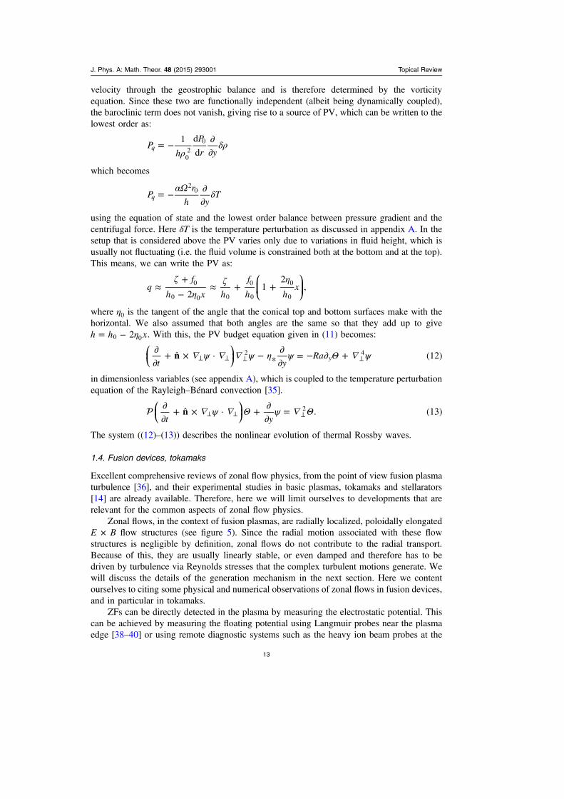
velocity through the geostrophic balance and is therefore determined by the vorticityequation. Since these two are functionally independent (albeit being dynamically coupled),the baroclinic term does not vanish, giving rise to a source of PV, which can be written to thelowest order as:

Ph

P

r y

1 d

dq

02

0

ρδρ= − ∂

∂

which becomes

Pr

h yTq

20αΩ

δ= − ∂∂

using the equation of state and the lowest order balance between pressure gradient and thecentrifugal force. Here δT is the temperature perturbation as discussed in appendix A. In thesetup that is considered above the PV varies only due to variations in fluid height, which isusually not fluctuating (i.e. the fluid volume is constrained both at the bottom and at the top).This means, we can write the PV as:

qf

h x h

f

h hx

21

2,0

0 0 0

0

0

0

0

ζη

ζ η≈

+−

≈ + +⎛⎝⎜

⎞⎠⎟

where 0η is the tangent of the angle that the conical top and bottom surfaces make with thehorizontal. We also assumed that both angles are the same so that they add up to giveh h x20 0η= − . With this, the PV budget equation given in (11) becomes:

t yRan · * (12)y

2 4ψ ψ η ψ Θ ψ∂∂

+ × − ∂∂

= − ∂ +⊥ ⊥ ⊥ ⊥ ⎜ ⎟⎛⎝

⎞⎠

in dimensionless variables (see appendix A), which is coupled to the temperature perturbationequation of the Rayleigh–Bénard convection [35].

t yn · . (13)2 ψ Θ ψ Θ∂

∂+ × + ∂

∂=⊥ ⊥ ⊥ ⎜ ⎟⎛

⎝⎞⎠

The system ((12)–(13)) describes the nonlinear evolution of thermal Rossby waves.

1.4. Fusion devices, tokamaks

Excellent comprehensive reviews of zonal flow physics, from the point of view fusion plasmaturbulence [36], and their experimental studies in basic plasmas, tokamaks and stellarators[14] are already available. Therefore, here we will limit ourselves to developments that arerelevant for the common aspects of zonal flow physics.

Zonal flows, in the context of fusion plasmas, are radially localized, poloidally elongatedE × B flow structures (see figure 5). Since the radial motion associated with these flowstructures is negligible by definition, zonal flows do not contribute to the radial transport.Because of this, they are usually linearly stable, or even damped and therefore has to bedriven by turbulence via Reynolds stresses that the complex turbulent motions generate. Wewill discuss the details of the generation mechanism in the next section. Here we contentourselves to citing some physical and numerical observations of zonal flows in fusion devices,and in particular in tokamaks.

ZFs can be directly detected in the plasma by measuring the electrostatic potential. Thiscan be achieved by measuring the floating potential using Langmuir probes near the plasmaedge [38–40] or using remote diagnostic systems such as the heavy ion beam probes at the


13

core of the plasma where the physical access is limited [41, 46]. However most measurementsof zonal flows in tokamak plasmas, is done on a particular class of oscillating zonal flows,called geodesic acoustic modes (GAMs). Because GAMs have a frequency of the order offew kHz in most tokamaks, they are much easier to detect. They have been observed on DIII-D [47, 48], JIPP T-IIU [49], ASDEX Upgrade [50], JFT-2M [51], T-10 [52], HL-2A [53] andrecently on Tore Supra using a special detection technique [54]. Note that, since theiroscillation is rather generic to toroidal geometry, we will not discuss specifics of GAMphysics in this review. Some aspects of GAMs are, nonetheless, similar to the low frequencyzonal flows that are related to the zonal flows that are observed in the geophysical setting.

Various diagnostic systems that measure fluctuation characteristics in tokamaks measuredensity fluctuations directly. These fluctuations show structures that propagate in the poloidaldirection. This apparent movement is due to a combination of wave propagation and theactual plasma velocity. While it is not possible to separate wave propagation and plasmavelocity looking only at density fluctuations, it is generally accepted that the radial profile ofthis speed corresponds roughly to the radial profile of the plasma velocity and the wave-number dependence of this observed velocity corresponds roughly to the wavenumberdependence of the phase speed, i.e.:

( ) ( )v r k v r v k, ( ) .fl E ph≈ +θ θ

Figure 6 shows the two dimensional profile of the poloidal velocity as inferred from themovement of density fluctuations observed using the beam emission spectroscopy system inthe DIII-D tokamak [37]. Here the shear in the radial direction comes mostly from the shear inthe E × B velocity.

1.5. Basic plasma devices

Zonal poloidal plasma flows have also been observed in various basic plasma devices, fromsmall stellerators such as CHS [41], TJ-II [42] and TJK [43] to linear machines such as CSDX[44], CLM [45] among others. Because of the relatively large values of collisionality, thedynamics in these small devices (in particular the linear ones) is mostly dominated by

Figure 5. A cartoon, showing the basic rotating convection pattern due to diamagneticdrift, temperature inhomogeneity and curvature in a tokamak, and the zonal flows thatare driven by the Reynolds stresses that are generated (in red).


14

Figure 6. The poloidal flow velocity associated with the zonal flow (GAM) in theD-IIID tokamak as inferred from the movements of density fluctuations measured bythe beam emission spectroscopy (BES) system [37].

Figure 7. Poloidal ion fluid velocity from CSDX, measured using a mach probe. Theoriginal figure in [55] also has error bars roughly of the order of ±50 m s−1 that wedropped for clarity.


15

dissipative drift instabilities (such as described by the Hasegawa–Wakatani system introducedin section 2.3.2). Using some heating schemes, ITG or electron temperature gradient driveninstability (ETG) modes has been reported in some of these basic devices. While stellaratorsmay appear relatively complicated for modeling, linear plasma machines can be modeledrather simply using a cylindrical geometry. A cylindrical plasma device with magnetic fieldalong its axis, is almost a one-to-one analogue to the rotating convection experimental setupdiscussed in section 1.3. Figure 7 shows the poloidal ion fluid velocity as a function of radiuswhere a ‘zonal jet’ (associated partly with the diamagnetic velocity due to background densitygradient) and smaller zonal flow structures can be observed.

2. Turbulence in fusion plasmas

The primary goal of the magnetic fusion programme is to achieve sufficiently long timeconfinement of plasma particles and heat so that the fusion reaction may start. This isachieved in tokamaks by keeping the effective diffusion of particles and heat across themagnetic field as small as possible. In modern fusion devices, collisions are fairly rare that theheat and particle transport they drive is feeble. This allows, by heating the core of the plasma,to enforce temperature profiles, where the plasma is very hot in the center, which is necessaryfor the fusion reaction, and relatively much colder where the plasma touches material sur-faces, which is important for the preservation of those surfaces. These radially inhomoge-neous profiles of temperature and density provide free energy sources for convectiveinstabilities akin to the convective instabilities in rotating convection problem describedabove (where physical rotation is replaced by diamagnetic rotation). These general class ofinstabilities are called drift-instabilities. They are classified based on the free energy source,rotation direction and the mechanism for tapping the free energy source.

As a general rule, radially inhomogeneous background profiles drive instabilities thathave an inward-outward fluctuating velocity component. This can be explained as the plasmatrying to get rid of the excess free energy (i.e. increase entropy), and in the absence ofmeaningful collisional transport, it can do so by arranging its fluctuating radial E × B flowsuch that the E × B flow is inward when the local temperature fluctuation is negative, andoutward when the local temperature fluctuation is positive (at least for the case when the freeenergy source is the temperature gradient). This way the hotter plasma is carried outward andthe cooler plasma inward, leading to an increase of entropy. This tendency, selects a linearlymost unstable mode with finite poloidal wavenumber k 0y ≠ , and usually a vanishing radialwavenumber k 0x = (where x is the radial direction as in the rotating convection problem).This mode that is linearly unstable is characterized by spatial patterns that can be called‘linear streamers’.

Starting from seed levels, such fluctuating flow patterns grow exponentially in time in thelinear phase, and saturate via mode coupling in the nonlinear phase. The couplings may beweak, nearly resonant triad interactions between well-defined waves, or strong interactions asin the case of fully developed turbulence, leading to a flux of energy, enstrophy etc through k-space. Furthermore, kinetic physics also contribute to this balance via resonant interactionsbetween waves and particles (Landau damping, Cerenkov emission etc).

Since the goal is the amelioration of confinement, and in the MHD sense a basic state ofconfinement is already achieved, the primary subject of plasma turbulence in magnetizedfusion is the study of the transport that the turbulence drives.


16

2.1. Description of plasma turbulence

While its classical description is rather simple, its collective nonlinear nature make the generalproblem of plasma turbulence, one of the most complex issues that the nature confronts uswith. It is, for instance, notably more complicated than the turbulence in neutral fluids due tocouplings to electromagnetic fields and kinetic effects such as Landau damping. There are apleithora of descriptions relevant for plasma problems, from the full Klimontovich descriptionto simple reduced fluid models such as Hasegawa–Mima or Hasegawa–Wakatani systems(see figure 8).

2.1.1. Klimontovich description. In a classical formulation, point particles follow trajectoriesthat are fully determined by the forces acting on them. Given a collection of such pointparticles, the probability of finding a particle at a given time at a given position with a givenspeed is either one or zero, depending on whether or not a particle trajectory coincides withthat point in phase space. This can be formulated using the probability distribution function

( ) ( )F t t tr v r r v v( , , ) ( ) ( ) , (14)s

j

N

j j

1

s

∑δ δ= − −=

where tr ( )j and tv ( )j constitute the trajectory of the jth particle. Taking the derivative of thisexpression with respect to time gives:

F

t t

F

t

Fr

r

v

v

d

d·

d

d· ,s

j

Nj s

j

j s

j

v

1

s

j⏞∑∂

∂=

∂∂

+∂∂=

⎛

⎝

⎜⎜⎜⎜

⎞

⎠

⎟⎟⎟⎟where the trajectories are determined by the equations of motion for the particles:

( ) ( ) ( )t

q

mt

ct t

vE r

vB r K r v

d

d, , , , (15)

j s

sj

jj s j j= + × ≡

⎡⎣⎢

⎤⎦⎥

Figure 8. The connections between different types of formulations in plasmaturbulence. The most general formulation being that of Klimontovich, and the simplestones being Hasegawa–Mima and reduced MHD. Only the crucial assumptions that arerequired are written at each step, even though there are others. BBGKY stand for theBogoliubov–Born–Greene–Kirkwood–Yvon hierarchy. One interesting observation isthat while rMHD seems to require a collisional fluid closure, one may obtain it alsobased on a large Magnetic field (which localize the particles, via Larmor rotation andplay the role of short mean free path).


17

with qs being the electrical charge for the species s, not to be confused with the PV (alsodenoted by q in this paper). Noting that F t F tr v r v( , , ) ( , , )j r rj

∑ = −∂∂

∂∂ and

F t F tr v r v( , , ) ( , , )j v vj∑ = −∂

∂∂

∂ , because of the form of (14), and using (15), we obtain

the Klimontovich equations:

F

t

Ft

Fv

rK r v

v· ( , , ) · 0. (16)s s

ss∂

∂+

∂∂

+∂∂

=

For each species s, which are coupled to the Maxwellʼs equations [56] for the fields with thesources given by:

( )t q q F tJ r v r r v r v v( , ) ( , , )d ,s j

s j j

ss s

3∫∑∑ ∑δ= − =

( )t q q F tr r r r v v( , ) ( , , )d .s j

s j

ss s

3∫∑∑ ∑ρ δ= − =

This formulation is in fact nothing but a trivial re-writing of the equations of motion in acompatible form with probabilistic descriptions. Thus, it provides no simplificationwhatsoever in the insurmountable initial task of solving Ns equations of motion for eachspecies coupled with the Maxwell equations.

One interesting, maybe somewhat philosophical point, is that turbulence as aphenomenon of multiscale disorder is nowhere to be found in this formulation of perfectlydeterministic motion of classical point particles. Nonetheless, the couplings between particlesin the above equation, which take place through Ks that is determined by the phase spacedistribution of all the other charged particles via the Maxwellʼs equations open the door to thepossibility of complicated motions that form the basis of what we call plasma turbulence.

2.1.2. Vlasov equation. One problem with the Klimontovich formulation, among others, isthat ( )F t F tr v r v r v( , , ) , , , , 0s s j j= ∣ depends on the initial positions and velocities of all theparticles of all species, since one needs the initial conditions for solving the equations ofmotion in order to find the trajectories. Since neither the determination of all the initialconditions, nor the computation of all the trajectories is possible, a statistical description is theonly option.

In order to achieve this, consider the average of ( )F tr v r v, , , , 0s j j∣ over a statisticalensemble of possible initial conditions:

( )f t F tr v r v r v( , , ) , , , , 0 .s s j j=

The distribution function f tr v( , , )s defined this way is naturally independent of the initialconditions, and is formally called a ‘single particle distribution function’. We can write downthe equation for the evolution of f tr v( , , )s by averaging the Klimontovich equation (16) overa statistical ensemble:

f

t

ft

Fv

rK r v

v· ( , , ) · 0. (17)s s

ss∂

∂+

∂∂

+∂∂

=

The Klimontovich acceleration involves only the electromagnetic fields that are solutions ofthe Maxwellʼs equations. Since those are linear, they can be solved using a response functionin terms of the charges and currents, which are themselves functions of the distributionfunction Fs. Therefore the last term in (17) describing the correlations between particles canbe reduced in two ways. If one drops correlations altogether, and considers only the mean


18

fields (that is the particles interact with eachother only via their interactions with thecollectively generated mean electromagnetic fields), one obtains the Vlasov equation:

f

t

f q

mt

ct

fv

rE r

vB r

v· ( , ) ( , ) · 0s s s

s

s∂∂

+∂∂

+ + ×∂∂

=⎡⎣⎢

⎤⎦⎥

in contrast, if one considers only local interactions (i.e. direct collisions), one obtains theBoltzman equation. In general, both of them together leads to the inclusion of a collisionoperator in the Vlasov equation above. Taking the moments of the Vlasov equation and usinga simple collisional closure, one can obtain different fluid closures such as the Braginskiiequations, or the two-fluid system of equations, which can be thought of as the basis forfurther reduction (see section 2.1.5 for a discussion).

2.1.3. Freezing in laws of two-fluid description. Consider the ion equation of motion:

t

e

m c

P

m nv v E

vB· (18)i i

i

i

i i

∂∂

+ = + × −⎜ ⎟ ⎜ ⎟

⎛⎝

⎞⎠

⎛⎝

⎞⎠

and continuity

tn nv v· · 0i i i i

∂∂

+ + = ⎜ ⎟⎛⎝

⎞⎠

for ions.Note that (18) is isomorphic to equation (1), with Lorentz force replacing the Coriolis

force. Taking the curl of the identity: v v v v v v( · ) 2 · 2 ( )= + × × wev v v vobtain [ · ] [ ( )]× = − × × × , which can be used to rewrite (18) as:

( )t m n

n Pv1

, (19)ig

i ig

i ii i2

Ω Ω∂∂

= × × + ×

where ig

ie

m c

B

iΩ ω≡ + is the ‘ion plasma absolute vorticity’, which is a sum of the ion plasma

vorticity vi iω = × and the cyclotron frequency e m cB i . Since (19) has the form of afreezing in law, we can write it as

t n m nn P

d

d·

1· . (20)i

g

i ii i2

χΩ

χ= × ⎛⎝⎜

⎞⎠⎟

Considering an equation of heat of the form

tP P Pv v· · 0.i iΓ∂

∂+ + =

Which actually implies conservation of:

tsv · 0,i

∂∂

+ =⎜ ⎟⎛⎝

⎞⎠

where s P n= Γ is the specific entropy. Now by choosing χ = s (or a function of s) causes theright hand side of (20) to vanish, resulting in the general definition of ion plasma PV as:

qn

s·i

ie

m c

i

B

iω

≡+

⎛

⎝⎜⎜

⎞

⎠⎟⎟


19

advected by the ion velocity vi. We will see later that simply using this definition with a driftapproximation, actually gives the correct definition of PV for various models such asHasegawa–Mima, Hasegawa–Wakatani or slab ITG.

Note that one can write a similar conservation law separately for the electron fluid,advected by the electron velocity

nev v

J,e i= −

where J is the plasma current density. Assuming for instance that the electrons have constanttemperature (or have a temperature proportional to their density):

q

e

m c

n

B

· ,e

ee

e

ωχ≡

−

⎛

⎝

⎜⎜⎜⎜

⎞

⎠

⎟⎟⎟⎟where χ is a constant of motion of the electron fluid.

2.1.4. Dual PV conservation in Hall MHD. If we consider the usual limit m me i≪ , and thedefinition of the v ve i

c B

ne4= −

π× , we can write dual freezing in laws as [57]

( ) j R Lu , ( , )t j j jΩ Ω∂ = × × =

with the pair of generalized vorticities and velocities defined as:

e

m c

c

ne

e

m c

Bu v B

Bv u v

,4

,

, ,

Re

R

Li

L

Ωπ

Ω

= = − ×

= + × =

where v, the ion velocity plays the role of plasma velocity. Since J· 0= , the equation ofcontinuity with the ion and electron fluids become the same with the quasi-neutralitycondition n ne i= :

n

tn

n

tnv v· ( ) · ( ) 0i e

∂∂

+ = ∂∂

+ =

which means that density is conserved both by ions and electrons, which allows us to write aPV pair:

qn

e

m c

c

ne

qn

e

m cs

Bu v B

Bv u v

1· ,

4

1· ,

Re

R

Le

L

χπ

= = − ×

= + × =

⎛⎝⎜

⎞⎠⎟

such that

tq j R Lu · 0, ( , ).j j

∂∂

+ = =⎜ ⎟⎛⎝

⎞⎠

Left fluctuations are expected to dominate the ion scales, while the right fluctuations dominatethe electron scales. This has actually been verified in a direct numerical simulation ofincompressible Hall-MHD [58].


20

2.1.5. Drift-fluid description and PV conservation. For spatial scales larger than the gyro-radius and time scales slower than the cyclotron frequency, one may consider the plasma as areduced fluid that moves around with drift velocities. The reduction that leads to this reducedfluid description is in fact a reduction in particle orbits approximating them using driftvelocities. Since the dynamics of its individual elements define the nature of a ‘fluid’ (as acontinuum approximation to a discrete system with very large degrees of freedom) the factthat the individual particles move in drift orbits leads to a description of a drift-fluid. Plasmain these scales act approximately as a drift-fluid as long as local kinetic equilibrium isestablished. In the case where kinetic physics is important, we use a drift-kinetic descriptionwhose moments would correspond to the drift-fluid description of desired complexitydepending on the closure of the fluid hierarchy.

One interesting aspect of reduced descriptions (especially for plasmas) is that multiplereductions based on very different assumptions may lead to same or very similar reducedmodels even though the justifications are based on completely different hypotheses. Oneexample is that, one can obtain reduced MHD equations either by making a fluid closure(strictly justified only when the collisions dominate) and than taking a strong magnetic field toforce the system to become 2D or directly by assuming a strong magnetic field and building afluid-like closure via the effect of the Lorentz force dominating the dynamics [59]. The reasonfor that is the second step making the first simplifying assumption obsolete, but somehow stillrespecting the final result (to a certain extent). So in this sense for instance the standard MHDmay be seen as an unnecessary but simplifying intermediate step.

In the same vein, the drift-fluid equations can actually be derived from two-fluid equations(which are normally justified based on collisional closures à la Braginskii). For this reason, somepeople call these drift-Braginskii closures. One may however also derive them by directly takingthe moments of the gyrokinetic equation leading to what is known as the gyrofluid [16]description and then going to the drift limit by dropping higher order finite Larmor radius effects.

Based on this justification, we will use two-fluid equations. An asymptotic expansion of thesmall parameter iω Ω (using the fact that the background magnetic field is very strong) leads towhat is known as the drift expansion. Doing this separately for ions and electrons and makingthe usual assumptions of quasi-neutrality and m me i≪ leads to simple tractable fluid models[60]. However, since the starting point for this derivation is the two-fluid equations. The exactconservation of PV for the two-fluid system leads to the conservation of an expandedapproximate PV for the drift-fluid, with an advection velocity given by the drift velocities.

For instance considering the dominant order ion velocity of the form v vi E= , where vE isthe E B× velocity gives directly:

t nv · 0E

i i

i

ζ Ω∂∂

++

=⊥⎜ ⎟⎛⎝

⎞⎠

⎛⎝⎜

⎡⎣⎢

⎤⎦⎥

⎞⎠⎟

now where v b· ˆi E

c

B2ζ Φ= × = ⊥ is the parallel component of the ion plasma vorticity,

and iΩ is the ion cyclotron frequency. It is interesting to note that this gives the Hasegawa–Mima equation that will be discussed in the next section when density is expanded as alinearly varying (i.e. in x) background and a small fluctuation around that. Note that in thisapproach, one need not to consider the nondivergence-free higher order correction to theplasma velocity (which is the polarization drift in the case of magnetized plasmas) explicitly.

2.1.6. Gyrokinetic equation and the PV. An honest description of turbulent phenomena infusion plasmas unfortunately requires a way to treat kinetic effects. In order to describekinetic evolution of plasmas under the influence of strong magnetic fields, we use the


21

gyrokinetic equation. Gyrokinetic equation in its full glory tends to be rather complicated.However in most cases it can be written in the form of a conservation law for the guidingcenter distribution function ( )F F X p t, , ,i i μ= ∥ :

( )( )t

B FX

XF Bp

p F B· ˙ ˙ 0,i i i* * *

∂∂

+ ∂∂

+ ∂∂

=∥ ∥∥

∥ ∥⎡⎣ ⎤⎦

where μ , the adiabatic invariant is simply a label (since td d 0μ = ). If we want to define aquantity similar to PV, we can define:

N B F vd di i*∫ μ≡ ∥ ∥

which is actually a normalized ion guiding center density. It becomes proportional to theusual PV in the limit of slab with adiabatic electrons and k 1sρ ≪⊥ .

2.2. Role of turbulence in fusion plasmas, turbulent transport etc

The possibility of transport driven by plasma microturbulence (called anomalous transportdue to historical reasons), and the difficulty this poses to the magnetized fusion was recog-nized rather early on in the development of the fusion programme. Different kinds ofinstabilities, with different characteristics have been identified over the years. One importantclass of instabilities that drive transport in tokamaks is the drift waves [61].

2.3. Drift waves, and instabilities

The basic drift wave is a density fluctuation on top of an inhomogeneous background densityprofile (see figure 9) that propagate because the radial fluctuating E × B velocity that this

Figure 9. The basic mechanism of the drift wave. Here filled contours of density isshown, which is the sum of a background profile decreasing in the x direction plus afluctuating sinusoidal component, which is proportional to the fluctuating electrostaticpotential due to the adiabatic electron response. This gives an E × B flow as shown,which is inward just below the density maximum and outward just above it. Since theoutward flow increase the density (by carrying high density plasma from the core) andthe inward plasma decrease it, the density maximum ends up moving upward.


22

density fluctuation generates, moves the high (low) density plasma outward just above adensity peak (hole), and low (high) density plasma inward just below it, leading to amovement of the density peak (hole) upward in the y direction.

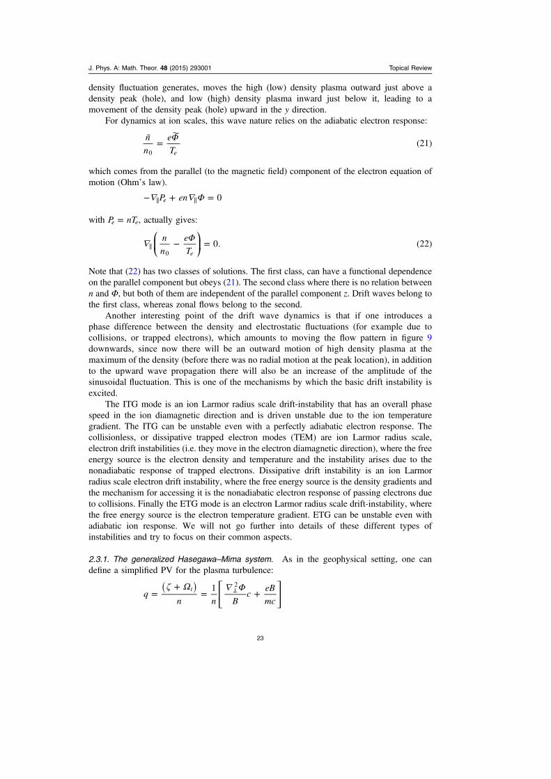
For dynamics at ion scales, this wave nature relies on the adiabatic electron response:

n

n

e

T

˜(21)

e0

Φ=

which comes from the parallel (to the magnetic field) component of the electron equation ofmotion (Ohmʼs law).

P en 0e Φ− + =∥ ∥

with P nTe e= , actually gives:

n

n

e

T0. (22)

e0

Φ− =∥⎛⎝⎜

⎞⎠⎟

Note that (22) has two classes of solutions. The first class, can have a functional dependenceon the parallel component but obeys (21). The second class where there is no relation betweenn and Φ, but both of them are independent of the parallel component z. Drift waves belong tothe first class, whereas zonal flows belong to the second.

Another interesting point of the drift wave dynamics is that if one introduces aphase difference between the density and electrostatic fluctuations (for example due tocollisions, or trapped electrons), which amounts to moving the flow pattern in figure 9downwards, since now there will be an outward motion of high density plasma at themaximum of the density (before there was no radial motion at the peak location), in additionto the upward wave propagation there will also be an increase of the amplitude of thesinusoidal fluctuation. This is one of the mechanisms by which the basic drift instability isexcited.

The ITG mode is an ion Larmor radius scale drift-instability that has an overall phasespeed in the ion diamagnetic direction and is driven unstable due to the ion temperaturegradient. The ITG can be unstable even with a perfectly adiabatic electron response. Thecollisionless, or dissipative trapped electron modes (TEM) are ion Larmor radius scale,electron drift instabilities (i.e. they move in the electron diamagnetic direction), where the freeenergy source is the electron density and temperature and the instability arises due to thenonadiabatic response of trapped electrons. Dissipative drift instability is an ion Larmorradius scale electron drift instability, where the free energy source is the density gradients andthe mechanism for accessing it is the nonadiabatic electron response of passing electrons dueto collisions. Finally the ETG mode is an electron Larmor radius scale drift-instability, wherethe free energy source is the electron temperature gradient. ETG can be unstable even withadiabatic ion response. We will not go further into details of these different types ofinstabilities and try to focus on their common aspects.

2.3.1. The generalized Hasegawa–Mima system. As in the geophysical setting, one candefine a simplified PV for the plasma turbulence:

( )q

n n Bc

eB

mc

1i2ζ Ω Φ

=+

= +⊥⎡⎣⎢

⎤⎦⎥


23

using

( )( )

qn B

ceB

mc

n Bc

n

eB

mc

x

L

n

n

1

1

1 11

x

L

n

n

n

0

2

0

2

0 0

n 0

Φ

Φ Φ

≈− +

+

≈+

+ + −∼

⊥

⊥

∼

⎛⎝⎜

⎞⎠⎟

⎛⎝⎜

⎞⎠⎟

whose conservation gives two equations when the fluctuating and mean components areseparated:

( ) ( )t L y

b bˆ · ˆ ·

(23)

s

n

2 2Φ Φ Φρ

Φ δ Φ Φ∂∂

+ × − + ∂∂

= × ⊥ ⊥ ⎜ ⎟⎛⎝

⎞⎠

tb bˆ · ˆ · , (24)2 2Φ Φ Φ Φ∂

∂+ × = − × ⊥ ⊥ ⎜ ⎟⎛

⎝⎞⎠

where ( )ab ab abδ ≡ − ⟨ ⟩∼ ∼ ∼∼ ∼ ∼, and we have used the adiabatic electron response (21) and

scaled temporal and spatial variables by i1Ω − and sρ respectively. We have also used the

dimensionless electrostatic potential e

Te

Φ . This system is called the generalized Hasegawa–Mima (or sometimes generalized Charney–Hasegawa–Mima) equations. Its nontrivialnonlinear structure follows from the fact that the electron response to the fluctuations areadiabatic, the electrons can not respond to Φ who is independent of the parallel coordinate.Note that a term similar to the last term on the left hand side of (23) is dropped from theequation for Φ , who is taken to be a function only of the radial coordinate x. However, formore general convective cells, such a term should be added to (24).

2.3.2. The Hasegawa–Wakatani system. Consider the PV for the drift wave problem:

( )q

n,

iζ Ω=

+

where cB

2

ζ = Φ⊥ as before, coupled to the equation for electron density (note that by quasi-neutrality n n ni e= = ), which can be written as:

tn

eJv ·

1E

∂∂

+ = ∥ ∥ ⎜ ⎟⎛⎝

⎞⎠

we can write the vorticity equation by eliminating the density from q td d 0= :

( )( )

t neJv ·E i

iζ Ωζ Ω∂

∂+ + =

+∥ ∥ ⎜ ⎟⎛

⎝⎞⎠

which basically says that the plasma absolute vorticity increases with a parallel current thatincrease with the parallel coordinate since such a current profile leads to an accumulation ofelectrons and thus an increase of plasma density. An increase in plasma density in turnincreases the vorticity, since the PV is conserved.

The Hasagawa–Wakatani system of equations follow if we use the Ohmʼs Law with afinite parallel resistivity instead of the adiabatic electron response:


24

e

TJ e

T

n

ne e 0

η Φ= −∥ ∥⎛⎝⎜

⎞⎠⎟

which gives:

( )t

nL

D n c nb · (25)s

ny

2 2Φρ

Φ Φ∂∂

+ × + ∂ − = −∼ ∼ ∼ ∥ ⎜ ⎟⎛⎝

⎞⎠

( )t

c nb · , (26)2 4 2Φ Φ ν Φ Φ∂∂

+ × − = − ∼ ⊥ ∥ ⎜ ⎟⎛⎝

⎞⎠

where we have scaled the parallel variable by Ln and defined cT

n L e

1

i

e

n02 2≡

Ω ηin addition to

using the dimensionless variables of section 2.3.1 and added model diffusion terms withdiffusion coefficients D and ν that are supposed to represent damping processes.

2.4. ITG

While a discussion of all the various different electrostatic micro-instabilities of the drift typein tokamaks is certainly out of the scope of this review, the ITG mode should probably bementioned as the most prominent ion Larmor radius scale instability.

The kinetic physics of the ITG mode is sufficiently complex that even the basic lineardispersion relation, with various usual simplifying assumptions such as adiabatic electronsand fluctuations being strongly localized to the low field side etc requires numerical approachfor finding the zeroes of a plasma dielectric function which has to be evaluated numerically.Furthermore, even such a (relatively complicated) numerical calculation is well known tooverestimate the growth rate of the ITG mode approximately by a factor of two. This meansthe full poloidal eigenmode problem has to be solved numerically. This is a rather fusionspecific exercise and has no place in a general review such as the current one.

While its accuracy in reproducing the linear physics would be poor, a reduced fluid ITGmodel can be used to study the nonlinear behavior of this mode. The use of such a model maybe justified retrospectively by the existence of zonal flows which tend to weaken thebalooning mode structure.

ITG requires either the parallel dynamics (cylindrical) or the curvature effects in order tobe unstable. We start with the PV budget (11) as in the rotating convection problem:

q

tP D

d

d,q q= −

where, we write the dissipation as D qq2ν= − ⊥ .

The PV for the simple slab ITG system can be defined as

( )q

P

n

i1ζ Ω

=+ Γ

considering ( )P P 1 x

L

P

P0P 0

= − +∼

, ( )n n 1 x

L

n

n0n 0

= − +∼

, and c

B2ζ Φ≈ :

qP

n

c

B

n

n

x

L

P

P

x

L1

1i

n P

01

0

2

0 0Φ Ω

Γ≈ + − − + −

∼

∼Γ

⎡⎣⎢⎢

⎛⎝⎜⎜

⎡⎣⎢

⎤⎦⎥

⎡⎣⎢

⎤⎦⎥

⎞⎠⎟⎟

⎤⎦⎥⎥

which basically is equivalent to q n P2Φ= − +Γ

in dimensionless form when the constantis dropped. The conservation of PV implies:


25

tn

P

L L yb · 0.s

n

s

p

2Φ ΦΓ

ρ ρΓ

Φ∂∂

+ × − + + − ∂∂

=∼ ∼ ⎜ ⎟⎛

⎝⎞⎠

⎡⎣⎢

⎤⎦⎥

⎛⎝⎜⎜

⎞⎠⎟⎟

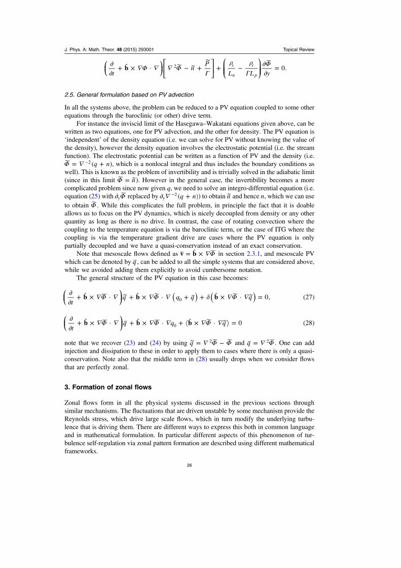
2.5. General formulation based on PV advection

In all the systems above, the problem can be reduced to a PV equation coupled to some otherequations through the baroclinic (or other) drive term.

For instance the inviscid limit of the Hasegawa–Wakatani equations given above, can bewritten as two equations, one for PV advection, and the other for density. The PV equation is‘independent’ of the density equation (i.e. we can solve for PV without knowing the value ofthe density), however the density equation involves the electrostatic potential (i.e. the streamfunction). The electrostatic potential can be written as a function of PV and the density (i.e.

q n( )2Φ = + − , which is a nonlocal integral and thus includes the boundary conditions aswell). This is known as the problem of invertibility and is trivially solved in the adiabatic limit(since in this limit nΦ = ∼ ). However in the general case, the invertibility becomes a morecomplicated problem since now given q, we need to solve an integro-differential equation (i.e.equation (25) with yΦ∂ replaced by q n( )y

2∂ +− ) to obtain n∼ and hence n, which we can useto obtain Φ . While this complicates the full problem, in principle the fact that it is doableallows us to focus on the PV dynamics, which is nicely decoupled from density or any otherquantity as long as there is no drive. In contrast, the case of rotating convection where thecoupling to the temperature equation is via the baroclinic term, or the case of ITG where thecoupling is via the temperature gradient drive are cases where the PV equation is onlypartially decoupled and we have a quasi-conservation instead of an exact conservation.

Note that mesoscale flows defined as v b Φ= × in section 2.3.1, and mesoscale PVwhich can be denoted by q , can be added to all the simple systems that are considered above,while we avoided adding them explicitly to avoid cumbersome notation.

The general structure of the PV equation in this case becomes:

( )( )t

q q q qb b bˆ · ˆ · ˆ · 0, (27)0Φ Φ δ Φ∂∂

+ × + × + + × =∼ ∼ ⎜ ⎟⎛⎝

⎞⎠

tq q qb b bˆ · ˆ · ˆ · 0 (28)0Φ Φ Φ∂

∂+ × + × + × =∼ ⎜ ⎟⎛

⎝⎞⎠

note that we recover (23) and (24) by using q 2Φ Φ= −∼ and q 2Φ= . One can addinjection and dissipation to these in order to apply them to cases where there is only a quasi-conservation. Note also that the middle term in (28) usually drops when we consider flowsthat are perfectly zonal.

3. Formation of zonal flows

Zonal flows form in all the physical systems discussed in the previous sections throughsimilar mechanisms. The fluctuations that are driven unstable by some mechanism provide theReynolds stress, which drive large scale flows, which in turn modify the underlying turbu-lence that is driving them. There are different ways to express this both in common languageand in mathematical formulation. In particular different aspects of this phenomenon of tur-bulence self-regulation via zonal pattern formation are described using different mathematicalframeworks.


26

3.1. Zonal flows and PV mixing

Various problems in geophysical fluid dynamics, plasma physics, and laboratory experimentsof rotating convection can be formulated using a PV quasi-conservation, where the injectionis via the baroclinic, or temperature gradient driven instabilities and the dissipation is due tosmall scale stresses. Therefore general rules about the tendencies of PV dynamics are veryuseful for understanding the common features of such systems.

One rather interesting, general observation of PV dynamics is that as long as the initialconfiguration has closed contours of time averaged PV (i.e. q q q0⟨ ⟩ ≡ + in the formulationof (27), (28)), the final state will consist of homogenized patches of PV connected by largegradients. Similar conclusion can also be drawn for contours of mean flow (streamlines),since to the lowest order these two are functionally related. This can be shown in differentways [1] here we only mention the demonstration using the integral around a closed PVcontour.

First note that the basic background steady state solution of (28), suggests that

qb · 0Φ× ≈

which means that to the lowest order, there is a functional relation between the mean PV andthe mean electrostatic potential:

( )q Q O ( ). (29)Φ ϵ= +

Note also that for any function f, the integral over an area A enclosed by a mean streamline

f s f ℓb bˆ · d ˆ · d 0, (30)A C

∫ ∮Φ Φ× = × =

where C is the closed contour around the streamline (i.e. ℓ ℓd dΦ Φ = ∣ ∣ ).Using this and (28), we can write:

q ℓb · d 0 (31)C

∫ Φ× ≈∼

in the steady state. Now using an eddy viscosity hypothesis:

qx

qb .i ijj

Φ κ× ∼ − ∂∂

∼

And the perturbation expansion (29), we can write

Q

x x

ℓd0

Cij

i j∫Φ

κ Φ ΦΦ

− ∂∂

∂∂

∂∂

≈

which implies that as long as ijκ is positive 0Q ≈Φ

∂∂

for any closed streamline. This means thatthe PV does not vary from one streamline to another on such a closed contour, which meansthat the steady state solution of the problem defined by (27) and (28) is simply:

q q q Oconst. ( )0 ϵ= + = +

in a region where the initial condition contained a closed contour of mean PV.However since this is in opposition to the background variation of the PV for example

due to background density gradient in the drift wave problem. The flat region of PV wouldhave to be connected to the next flat region by a strong gradient. When many of such regionsare connected, the result is what can be called a PV staircase.

Notice that the nonlinear term vanishes for a homogenized PV profile. There is a closeanalogy between the homogenization of the PV and the phenomenon of flux expulsion in


27

MHD and eventually to the phenomenon of dynamic alignment which leads to generation oflarge regions of aligned or counter-aligned velocity and magnetic field profiles which areconnected by sheets or filaments where the alignment changes rapidly.

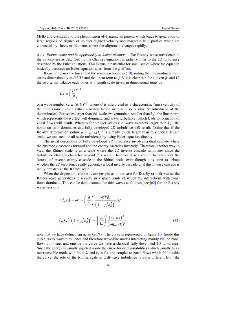
3.1.1. Rhines scale and its applicability to fusion plasmas. The Rossby wave turbulence inthe atmosphere as described by the Charney equations is rather similar to the 2D turbulencedescribed by the Euler equations. This is true in particular for small scales where the equationbasically becomes an Euler equation apart from the β effect.

If one compares the linear and the nonlinear terms in (10), noting that the nonlinear termscales dimensionally asU L2 2 and the linear term as Uβ′ it is clear that for a given β′ and U,the two terms balance each other at a length scale given in dimensional units by:

LU

R

1 2

β≡

⎛⎝⎜

⎞⎠⎟

or a wave-number k U( )R1 2β≡ , where U is interpreted as a characteristic (rms) velocity of

the fluid (sometimes a rather arbitrary factor such as 2 or π may be introduced at thedenominator). For scales larger than this scale (wavenumbers smaller than kR), the linear termwhich represents the β effect will dominate, and wave turbulence, which leads to formation ofzonal flows will result. Whereas for smaller scales (i.e. wave-numbers larger than kR), thenonlinear term dominates and fully developed 2D turbulence will result. Notice that if theRossby deformation radius R h g f0 0

1= − is already much larger than this critical lengthscale, we can treat small scale turbulence by using Euler equation directly.

The usual description of fully developed 2D turbulence involves a dual cascade wherethe enstrophy cascades forward and the energy cascades inversely. Therefore, another way toview the Rhines scale is as a scale where the 2D inverse cascade terminates since theturbulence changes character beyond this scale. Therefore it is common to talk about the‘arrest’ of inverse energy cascade at the Rhines scale, even though it is open to debatewhether the 2D turbulence really generates a local inverse cascade or if this inverse cascade isreally arrested at the Rhines scale.

When the dispersion relation is anisotropic as in the case for Rossby or drift waves, theRhines scale generalizes to a curve in k space inside of which the interactions with zonalflows dominate. This can be demonstrated for drift waves as follows (see [62] for the Rossbywave version):

( )u k

L

k

k1rms R

s

n

s Ry

s R

i2 2 2

2 2 2

2 2 22ω

ρ ρ

ρΩ= =

+

⎛⎝⎜

⎞⎠⎟

( )( ) ( )( )

k kL e T

1sin

(32)s R s Rs

n

R

rms e

2 2 2 22 2

2ρ ρ

ρ α

Φ+ =

⎛⎝⎜

⎞⎠⎟

note that we have defined k ksin R Ry Rα ≡ . The curve is represented in figure 10. Inside thiscurve, weak wave turbulence and therefore wave-like modes interacting mainly via the zonalflows dominate, and outside the curve we have a classical fully developed 2D turbulence.Since the energy is usually injected inside the curve for drift instabilities (which usually has amost unstable mode with finite ky and k 0x ≈ ), and couples to zonal flows which fall outsidethe curve, the role of the Rhines scale in drift-wave turbulence is quite different from the


28

arrest of the 2D inverse cascade picture. Note that as an order of magnitude

( )( )e Te Lrms2 2

s

nΦ ∼ ρ

in drift wave turbulence (i.e. the mixing length estimate).

While the applicability or the importance of the Rhines scale to fusion plasma turbulencemay be questionable, the curve given in figure 10 can be interpreted as the boundary betweenanisotropic turbulence at ‘large’ scales and the isotropic turbulence at ‘small’ scales. Whenthe energy is injected within the above curve, it will excite a drift wave which has the form ofa streamer (i.e. k kx y≪ mode), this mode couples naturally to an isotropic mode (withk kx y∼ , sometimes called a Kelvin–Helmholtz-like mode, but we think that this terminologyis misleading) and a zonal mode. The interaction in a fusion device is actually a 4-waveinteraction where the two satellites of the primary pump mode (i.e. the streamer) couple togive the zonal mode. We will discuss how this can be described in the framework ofmodulational instability in the following sections.

However note that as the energy goes to the zonal flow, the zonal flow transfers some ofthis energy to a smaller (or larger) scale k kx y∼ mode and a smaller (or larger) scale streamer-like mode. Sometimes called a tertiary instability. However since the smaller scale streamerthat is driven by the ‘tertiary instability’ then drives smaller scale zonal flows leading to acascade of enstrophy through the k-space via these particular triads, it is in fact simply a partof an hierarchy of interactions. We think that within the context of turbulence calling it an‘instability’ is misleading unless one sees each step in the cascade as an instability of theprevious scale. In contrast it is clear that for single wave-packet whose characteristics actuallyevolve in time, the tertiary instability has a clear meaning.

3.1.2. Rhines scale versus mixing length versus critical balance. There are various examplesin the literature where people consider the balance between the linear and the nonlinear termsas we have discussed above to define the Rhines scale. The mixing length idea commonlyused in fusion to estimate the fluctuation level is indeed a balance between the linear and thenonlinear terms. For instance for the Hasegawa–Mima case:

L y

e

T

e

T

e

Tb ·s

ns s

4 2ρ

ρ Φ ρ Φ Φ∂∂

≈ ×

⊥ ⎛⎝⎜

⎞⎠⎟

⎛⎝⎜

⎞⎠⎟

⎛⎝⎜

⎞⎠⎟

Figure 10. Anisotropic Rhines scale for drift wave turbulence. Inside the curve, theturbulence has a wave-like character and interactions with the zonal flows dominate,outside it has the character of a classical fully developed 2D turbulence.


29

which gives (for k k 1s s yρ ρ∼ ∼⊥ which is roughly true for the most unstable mode):

e

T Ls

n

Φ ρ∼

this is the basic mixing-length estimate of the fluctuation level for drift-wave turbulence. Amore detailed version can be used to determine the maximum of the turbulence k-spectrum byarguing that the maximum occurs when the linear growth rate is balanced by the nonlineardecorrelation rate (i.e. eddy damping):

D k ,k knl 2γ ≈ ⊥

where Dknl e

T2k∝ ∣ ∣Φ is the nonlinear diffusion coefficient that appears in turbulent fluxes of

density and particles [63]. The maximum of the spectrum can be obtained by solving:

e

T kmax maxk k

2

2

Φ γ≈

⊥

⎛⎝⎜⎜

⎞⎠⎟⎟

⎛⎝⎜

⎞⎠⎟

for k. Since the functional form of kγ can in principle be obtained maximizing kk2γ ⊥ one

obtains the mixing length maximum of the spectrum. It is interesting to note that this seems towork rather well for turbulence in tokamak plasmas even with the complicating effects ofcurvature, magnetic shear etc [124]. The reason is probably that most of the complicatingeffects change the form of kγ in this argument, but do not change the fact that the kγ isbalanced by an effective turbulent diffusion near the most unstable mode. Note that while oneuses the same basic idea of balancing linear and nonlinear terms, the mixing length considersthe energy budget (so the energy injected by the linear instability is equal to the energyextracted by the nonlinear transfer), whereas the Rhines scale argument is based on acomparison between the eddy turnover rate and the wave propagation in the original equation.

Yet another famous balance between the linear and the nonlinear terms is the so-calledcritical balance [64] in 3D MHD turbulence. The idea is very similar to how one obtains theRhines scale but considering parallel propagating Alfvén waves with a fully developed 2Dperpendicular spectrum. By balancing the Alfvén wave transit rate in the parallel directionwith the eddy turnover rate in the perpendicular direction, one obtains:

( )v k u k k .A ≈∥ ⊥ ⊥

Notice that in standard 3D MHD there is no process which would break the isotropy on theperpendicular plane (i.e. kx versus ky), however there is a rather important source ofanisotropy in the parallel versus perpendicular directions. Since the spectral energy density inthe perpendicular direction for a 2D forward cascade is ( )E k k2 3 5 3ε∝⊥ ⊥

− or

( ) ( )u k E k k k ,1 2 1 2 1 3 1 3ε∼ ∝⊥ ⊥ ⊥ ⊥− the critical balance gives the relation:

kv

k .A

1 32 3ε∝∥ ⊥

This is usually interpreted as a strongly anisotropic spectrum with k∥ following the k⊥ cascadescale by scale until it reaches the critical balance. It can be generalized for an arbitrarydispersion relation by replacing vA with the parallel phase velocity v k( )ph∥ . The idea can beapplied to various systems with parallel propagating waves.

3.1.3. PV and its importance in DW/ZF dynamics. As discussed above, a number of plasmaand geophysical fluid dynamics models can be formulated using a description based on PV


30

evolution. Advection of PV, coupled to other equations such as that of entropy density orpressure via the baroclinic term or via curvature effects when there are additional sources offree energy. Notice however that in general the quadratic quantity that is conserved by thenonlinear dynamics of co-evolving drift waves and zonal flows, as described for instance by(23) and (24), is the PE.

( )W q q q 1 .2 2 2 22

2 2Φ Φ≡ = + = − +∼

In other words the nonlinear system described by (23) and (24), the zonal flows and the driftwaves exchange PE and not energy. So it is the PE that is conserved between the drift wavesand the zonal flows, since it is the PV that is advected. However local interactions among thedrift waves still conserve energy and enstrophy leading to a dual cascade.

3.1.4. Forward enstrophy cascade and ZF formation. One interesting point is that while it iscommon to talk about zonal flow formation informally as a process of ‘inverse cascade’, in

Figure 11. Forward potential enstrophy cascade mediated by large scale flow structures.

Figure 12. Simple mechanism for the zonal flow reinforcement.


31

reality the anisotropic mechanism that leads to the formation of zonal flows does not reallyhave the character of a local cascade where the energy moves to larger and larger scales. Themechanism can be described better as a nonlocal interaction in k-space where the zonal flowacts on all scales diffracting the fluctuations to smaller and smaller wave-numbers (seefigure 11).

From a spatial, ’pattern formation’ point of view, the same process can be explained bylooking at the dispersion relations for drift or Rossby waves. Consider the setup in figure 12,for Rossby waves as the first example. The basic Rossby wave has a mainly westward phasemotion, with a phase velocity given by:

k

kv kx

ph 4

β= −

′

while its latitudinal group velocity, vgx, can be in either direction, its meridional groupvelocity, vgy, is in the opposite direction to its meridional phase velocity, making it abackwards wave in the meridional direction:

vk

k

k

k k

k

2.gy

y

x x y

2 4

β β= ∂

∂−

′=

′⎛⎝⎜

⎞⎠⎟

Similarly for drift waves the main phase velocity propagation direction is counter-clockwisein the geometry of figure 12 if the magnetic field is in the out of plane direction. The radialgroup velocity

( ) ( )v

k L

k

k L

k k

k

d

d*

1*

2

1gx

x n

y

n

x y

2 2 2

ρ ρ=

+= −

+

⎡

⎣⎢⎢

⎤

⎦⎥⎥

which is also backwards with respect to its radial phase propagation (i.e.( )

v *x L

k k

k kph

1n

y x

2 2= ρ

+).

Note that while Rossby waves carry negative wave momentum away from the stirring region,the drift waves carry positive wave momentum towards the stirring region resulting in thesame basic effect of momentum convergence towards this region.

One very interesting point is that if an infinitesimal velocity shear which has the profilegiven in figure 12 is introduced, the sheared flow leading to a tilting of the eddies resulting ina radial (meridional in the case of Rossby waves) group propagation which leads tomomentum convergence towards the maximum of the flow.

3.2. The wave-kinetics formulation

Self-regulating drift/Rossby wave turbulence, can be described using the wave kineticequation in a weakly inhomogeneous medium [65–67]:

( )

( ) ( )tN t N t

N t C N N

X V k X

V k X

( , ) · · ( , )

· · ( , ) , , (33)

Xk k k

X k k k k

ω

ω

∂∂

+ −

− − = ′

⎡⎣ ⎤⎦⎡⎣ ⎤⎦

where Nk is the wave quanta of the drift waves. The weak inhomogeneity described partly bythe dispersion relation and partly by the mean flow V above can be coupled to the slower timescale evolution of the zonal flows using a scale separation approach. Notice that it is alsopossible to obtain the wave kinetic formulation, and derive explicit expressions for thediffusion coefficients using a Lagrangian correlations approach [68, 69].


32

When considered by itself the wave-kinetic equation describes the evolution of highfrequency drift waves that move around in a medium whose optical index of refraction isdetermined by the zonal shearing. Recall that the WKB equations can be written as

( )t

xk

V kd

d·kω= ∂

∂−

and

( )t

kx

V kd

d·kω= − ∂

∂−

which is the basis for the interpretation of (33) as a ‘kinetic’ equation. Notice that since zonalflows are narrow banded flow structures, they play the role of wave-guides for drift waves.

The wave kinetic formulation of drift-wave zonal flow interaction is a very powerful tool.As discussed in detail in reference [36], a quasi-linear calculation, based on the wave-kineticformulation (i.e. using N N Nk k kδ= ⟨ ⟩ + where Nkδ is a perturbation) can be used to estimatethe zonal flow ‘growth rate’ (i.e. the rate at which the zonal flows are driven by drift waves):

( )[ ]W q c

k

kR k q k

kW2

1( , ) ,q k s

k

y s

s

xx

k2 2

2 2

2 2 2∑γ

ρ

ρ= −

+

∂∂

where ( )W k1k s k2 2 2 2ρ Φ= ⟨ + ∣ ∣ ⟩ is the drift wave PE density. Remarkably, the general form

of the coupled quasi-linear system of equations that result:

tW

kD

kW W

NW , (34)k

rk

rk k k

kk

0

2γΔω∂

∂− ∂

∂∂

∂= −

⎡⎣⎢

⎤⎦⎥

[ ]t

W . (35)q q k q d q nl q q2 2 2 2 2Φ γ Φ γ Φ γ Φ Φ∂

∂= − − ⎡

⎣⎢⎤⎦⎥

A formal statistical calculation based on the direct interaction approximation betweendisparate scales for the generalized Hasegawa–Mima system gives essentially the same resultalso [70]. Notice that the equations (34) and (35) already suggest

(i) that the turbulence drives zonal flows via qγ ,(ii) that the zonal flows contribute to the forward enstrophy cascade by refracting the drift

waves towards smaller kr. Adding the zonal flow damping, we have roughly all theingredients for a spectral PP dynamics as described in figure 11.

3.3. Modulational instability framework

Assuming that the spatio-temporal dynamics of large scale flow structures is sufficientlyslower than that of drift/Rossby wave turbulence, one can use the modulational instabilityframework. The complete framework can actually be developed from a Hamiltoniandescription of nonlinear waves, for which there are already very good books and reviews[71, 72]. Since, the purpose of this paper is to review physical mechanisms, we limit our-selves to a discussion of the modulation instability and discuss the formulation by Newell[73]. Consider the nonlinear system

( )R, , , (36)t ϕ ϕ ϕ∂ =

where , and are operators representing linear terms and nonlinear couplingsrespectively, and R represents a parameter that determines the stability condition (e.g. the


33

Rayleigh number for the problem of convention). We obtain the linear dispersion relation forgiven R by linearizing (36):

Rk(i , i , ) 0, (37) ω− =where irk k kω ω ω γ= ≡ + is the complex frequency. One can obtain the stability conditionby substituting R( )kω ω= and setting 0kγ = , and solving for R R k( )c= instead.

In many problems in nature there is a critical scale (the most unstable mode) at which thenet energy production has a maximum because the energy production decreases towardslarger scales, and the dissipation increases towards smaller scales. This implies that R k( )c hasa minimum at this point. Thus, when the control parameter R is close to, but slightly above itscritical value

( )R R 1c2ϵ χ= +

only a small subset of modes around the most unstable mode are excited (i.e. k O ( )c ϵ± ). Thisallows us to consider a wave whose amplitude is slowly modulated:

( )X T, , e c. c .,tk xi · i ˜rkϕ Φ τ= +ω−∼

where X T( , , )Φ τ is the modulated complex amplitude, using the reductive perturbationtheory:

( )0 12

2ϕ ϵ ϕ ϵϕ ϵ ϕ= + + + ⋯

with a basic scale separation assumption, which can be regarded as a Taylor series expansionof the operator 0 1

22 ϵ ϵ= + + + ⋯, around the point R( ˜ , ˜ , )t c∂ to a neighboring

point ( )R˜ ¯ , ˜ ¯ , 1t T c2 2ϵ ϵ ϵ ϵ χ+ ∂ + ∂ + ∂ +τ ⎡⎣ ⎤⎦ in the operator space. For example

( )

R R

R

k k

kk

v

(i , i , )

( i )¯ (i , i , )

(i )· ¯

(i , i , )

( i )¯ · ¯ , (38)

T

T g

10 0

0

ωω

ω

ωω

=∂ −

∂ −∂ +

∂ −∂

=∂ −

∂ −∂ +

⎛⎝⎜

⎞⎠⎟

where we have used the fact that

R Rk

kk

k(i , i , ) (i , i , )0 0 ω ωω

ω∂∂

− = − ∂∂

∂∂

−

which can be obtained by differentiating the dispersion relation (37). Note that (38)corresponds to the group motion of the envelope modulation and can be eliminated bytransforming to a frame of reference moving with the group velocity.

Similarly

k k ki

RR

1

2¯ ¯ 1

2¯

(39)

TTi

T ii j

i j2

20

2

20

20 0 0

ω ω ωχ= −

∂∂

∂ +∂∂ ∂

∂ ∂ −∂

∂ ∂∂ ∂ +

∂∂

∂ +∂∂τ

substituting the following relation, which can be obtained by taking the second derivative ofthe dispersion relation with respect to k:

k k k k k k k k

R

k k R

1

2

1

2

1

2

1

2(40)

i j i j i j i j i j

20

20

20

2

20

20 ω

ωω ω

ωω

ω−

∂∂ ∂

= ∂∂ ∂

∂∂

+ ∂∂

∂∂

∂∂

+ ∂∂

∂∂ ∂

+ ∂∂ ∂

∂∂


34

and using the transformation to the group velocity frame that was used to eliminate 1 (i.e.

T k ii

∂ = − ∂ω∂∂

), we note that the first and second terms of (39) are canceled by the second andthe third terms on the right hand side of (40) respectively. This leaves:

k k

R

k k R RRi ¯ 1

2

1

2(41)

i ji j

i ji j2

02

02

0 0 ω

ωω

χ=∂∂

∂ + ∂∂ ∂

∂∂

∂ ∂ + ∂∂ ∂

∂∂

∂ ∂ +∂∂τ

which is to be balanced by the nonlinear terms. The exact form of the resulting equationsdepend on the details of the nonlinear saturation mechanism that balances the envelopemodulations that can be described in general using the above formalism. The envelopeequation, including the lowest order nonlinear terms takes the form

.2 0 0 0 0 0 Φ Φ Φ≈

The simplest possible example that results in various physical problems is the so callednonlinear Schrödinger equation, which takes the form:

k xi ¯

1

2

d

d0,

2

2

2

22Φ ω Φ λ Φ Φ∂ + ∂

∂+ =τ

where λ is the lowest order coefficient for the perturbation expansion of the nonlinear term.The nonlinear Schrödinger equation is common to a number of interesting physical problems,and its implications are profound. Another thing that is very remarkable about this equation isthat, it has actually been solved using the inverse scattering method, which were later ondeveloped into a methodology for solving similar equations. However here we only use it asan example to the large class of possible amplitude equations that can be obtained from themodulational instability framework and refer the reader to the well written books and reviewpapers on the subject [125].

3.3.1. Amplitude equations and their application to basic zonal-flow/drift-wave system.Consider the nonlinear system (23)–(24) which describes the coupled evolution of simpledrift-waves and zonal flows. We can write (23) in the form:

( ) ( )b bˆ · ˆ · ,2 2Φ Φ Φ Φ δ Φ Φ= − × − + × ⊥ ⊥

where the linear dispersion relation follows from:

( )( ) kL

kki , i i 1 0k ks

ny0

2 ω ωρ

− = − + + =

which gives:

( )( ) kki , i i 1 .k

k02

ωω∂

∂− = − +

Note that for this problem, there is no R, since the basic linear dispersion relation is alwaysstable.

Using the reductive perturbation method described above, considering zonal modula-tions, and flows (i.e. 0Y∂ → ) and assuming further that the zonal electrostatic field variesroughly at the same scale at which the envelope is modulated (i.e. X T( , , )e tk x

0 0i( · )Φ Φ τ= ω−

and X T( , )Φ Φ= ), we can write for 2 from (41):


35

k kki

1

2(42)

x xXX y X

2ω Φ Φ Φ∂ + ∂∂ ∂

∂ = ∂τ⎛⎝⎜

⎞⎠⎟

which is then coupled to

( )v k k2 . (43)gx X XX x y XX2ϵ Φ Φ∂ − ∂ ∂ = ∂τ

Note that a scaling O ( )Φ ϵ∼ , O ( )Φ ϵ∼ is suggested if the term on the right hand side of(42) is to be of the same order as the term on the left hand side, while the group velocity termin (43) is to be of the same order as the term on the right hand side. In this case we can solve(43) by neglecting the the higher order ϵ∂τ term and substitute the result into (42), whichgives:

k k

k k

vi

1

2

20 (44)

x xXX

x y

gx

2 22Φ ω Φ Φ Φ∂ + ∂

∂ ∂∂ + =τ

which is again the nonlinear Schrödinger equation (NLS), which we write as

i 0, (45)XX2Φ β Φ α Φ Φ∂ + ∂ + =τ

where

k k

k k

v

1

2and

2. (46)

x x

x y

gx

2 2

β ω α≡ ∂∂ ∂

≡

Consider the following perturbed homogeneous solution:

( )e0i 2Φ Φ δΦ= + α Φ τ

which, without the δΦ is a homogeneous plane wave with a nonlinear frequency shift.Looking at the linear stability of ( )e q X

0i x ZδΦ δΦ∼ ω τ− , one obtains the dispersion relation:

q q2 .zf x x2 2 4 2

02ω β αβ Φ= −

The instability condition for this dispersion relation is basically that

q 2x2

02α

βΦ<

when the mode is unstable, we can write:

( )q q q2zf x x x2

02 2 4γ αβ Φ β= −

which allows us to compute the most unstable zonal mode, (i.e. by setting ( )q 0zf xγ′ = ):

q (47)x2

02α

βΦ=

and with this the growth rate of the most unstable mode:

( )( )qc k k

L

e

T

1zf x

s y s

s n e0

22 2 2

02

γ α Φρ

ρΦ

= =+

in dimensional form.It is interesting to note that, the modulational instability framework, defines a specific

characteristic ‘most unstable’ wave-number for the zonal flows (i.e. (47)). While the final‘steady state’ (if there ever is a steady state) value of the zonal flow wave-number depends


36

also on the way it is dissipated, which we will discuss in section 4, the most unstable wave-number would give an indication about the characteristic radial size of the zonal flows. It isinteresting to note that as to the knowledge of current authors, this was never used as a basisfor comparison, at least in fusion experiments.

3.4. Pattern selection in electron scales by modulational instability

Using the general framework of modulational instability, we consider a two field model ofsmall scale drift turbulence driven by ETG. Both because it was done initially for this systemand due to the its direct similarity to the rotating convection problem discussed in section 1.3.Here we also demonstrate the application of the modulational instability framework to thequestion of 2D pattern selection in plasma turbulence. We consider a reduced fluid ETGsystem as a working model:

( )( ) Pz · 1 ( ) 0, (48)t y2 4Φ Φ Φ ν Φ∂ + × − + ∂ + + =

( )P P rz · 0, (49)t y2Φ χ Φ∂ + × − − ∂ =

where the following dimensionless drift wave variables are used:

e

TP

P

Pt t

L

v

c L

v

c

L

v

cr

x x*

, , * ,

** , *

* ,

, *

i i

B e

i ie i e

ie

n

i

see

e

p

e

se

Be

B

B

se

B e

i

1

*2

0

*2

e

Φ ϕϵ

ϵϵ

Ω ϵ τ ρ

ϵτ ρ

ϵτ ρ

ϵτ ρ ϵ ϵ

ϵ

→ → → →

= = = − =

= = =

and T Ti eτ = . In order to apply the modulational instability framework, we separate thefluctuations and mean flows/fields. The mean flow equations, dropping the dissipative terms,can be written as

( ) ( )P z1 ¯ ¯ ¯ ˆ ˜ · ˜ , (50)T Y2 2Φ Φ Φ Φ∂ − + ∂ + = ×

P r Pz¯ ¯ ˆ ˜ · ˜ , (51)T YΦ Φ∂ − ∂ = ×

and the two equations for the fluctuations can be combined as:

( )

( )

( )

( )

( )( )

( )

( )

r

k rk k Pz k

1

ˆ · 1 2 ¯ ¯ 0 (52)

t t y yy

L

y y y

N P

2

, ,

2

¯, ¯

t y x

Φ ω Φ Φ

∂ ∂ − + ∂ + ∂

× − × + − − =

Φ

∂ ∂ ∂

⎡⎣ ⎤⎦

by dropping the direct interactions between fluctuations and dissipation.The Reynolds stress for a modulated monochromatic wave in general can be written as:

( )( )

z z k k

z k J k J

ˆ ˜ · ˜ 2 ˆ · ( · )

ˆ · ( · ) ( · )( ) , (53)z

2 2Φ Φ Φ× ≈ ×+ × − ×


37

where,

( )J i * *Φ Φ Φ Φ= −

is the Schrödinger intensity flux density, and Φ is the complex amplitude. Similarly for theadvection of pressure,

( )P P P P Pz z k zˆ ˜ · ˜ · ˆ i * * ˆ * * . (54)Φ Φ Φ Φ Φ× ≈ × − + × − ⎡⎣ ⎤⎦ ⎡⎣ ⎤⎦The phase difference between Φ and P can be calculated from (49), by including slowmodulations. When we consider a particular perturbation expansion (53) and (54) will befurther simplified.

It is easy to see, from (52) that the linear dispersion relation has two solutions, and theunstable mode has a maximum at k 0x = . This means that the monochromatic drift-wavearound which we perform the modulational instability has k 0x = but finite ky.

3.4.1. Initially isotropic modulations. In order to see what kind of elongated patterns formamong zonal flows with X YΔ Δ≪ , streamers with X YΔ Δ≫ , or isotropic convective cellswith X YΔ Δ∼ , we start the analysis with isotropic modulations and see in which direction thesystem evolves. The amplitude equation in this case can be written as:

( )k k

ki1

2

1

20. (55)

yYY

xXX y XX

2

2

2

22 2Φ ω Φ ω Φ α Φ Φ∂ + ∂

∂∂ + ∂

∂∂ + ∂ =τ

It is also possible to rewrite this with the scalings X X xβ→ ∣ ∣ , Y Y yβ→ ∣ ∣ ,k( )y xΦ α β Φ→ ∣ ∣ , where k(1 2)x x

2 2β ω= ∂ ∂ and k(1 2)y y2 2β ω= ∂ ∂ , and replacing

*Φ Φ→ if 0xβ < , which gives:

( )i . (56)YY XX XX2Φ Φ Φ σ Φ Φ∂ + ∂ + ∂ + ∂τ

This scaling uses the fact that the signs of xβ and yβ are the same. Here 1σ = ± is the overallsign of ( )xα β , where 1σ = − corresponds to an attractive nonlinearity and σ = +1 to arepulsive one. The total Hamiltonian for (56):

( )( )H Vd2

(57)X Y X2 2 2

2∫ Φ Φ σ Φ= ∂ + ∂ + ∂⎡⎣⎢

⎤⎦⎥

is conserved. Following Talanov, we write the evolution equation for the radial and poloidalvariance (defined as X X X Yd d2 2 2∫ Φ⟨ ⟩ = ∣ ∣ and Y Y X Yd d2 2 2∫ Φ⟨ ⟩ = ∣ ∣ respectively):

( )( )X

tH X Y

d

d4 4 d d , (58)X X Y

2 2

22 2 2 2∫ σ Φ Φ Φ= + ∂ + ∂ − ∂

⎡⎣⎢

⎤⎦⎥

Y

tH X Y

d

d4 4 d d . (59)Y X

2 2

2

2 2∫ Φ Φ= + ∂ − ∂⎡⎣ ⎤⎦As these are explicit differential equations for the second derivatives of these quantities

(akin to acceleration), one may qualitatively interpret them as Newtonʼs equations of motion.For H 0< , which is possible for σ = −1, the total variance V is always ’pulled’ towards zero,leading to a collapse. However it is easy to see that for H 0< V Vx y− is always ’pulled’

towards the negative axis. This means X 2⟨ ⟩ is always ‘pulled’ more strongly than Y 2⟨ ⟩. Sincean initially isotropic state corresponds to X Y2 2⟨ ⟩ ∼ ⟨ ⟩, one arrives at the conclusion that the


38

final state will have X Y2 2⟨ ⟩ ≪ ⟨ ⟩ or X Y∂ ≫ ∂ . Notice that H 0< is a condition on the initialdata that allows the finite time singularity formation.

The collapse of the initial data to a singular layer in the perturbation analysis suggeststhat the wave amplitude becomes larger and X∂ becomes smaller than it is assumed in theperturbation expansion corresponding to the initial isotropic modulation. The completeevolution of an initially isotropic amplitude modulation can be seen in figure 13. Theperturbation expansion breaks down as the system collapses in the radial direction, resultingin a poloidally elongated (i.e. X Y∂ ≫ ∂ ) modulation (and flow) structure. However, we cancontinue the analysis by choosing a new scaling.

3.4.2. Further anisotropic evolution. An equation describing the further evolution of thestructure in the limit X Y∂ ≫ ∂ may be derived similarly to the isotropic case. The mainproblem is that if the scaling is such that Y X

2∂ ∼ ∂ , one can no longer neglect the divergence ofintensity flux density term k J( · )y x∂ in the calculation of the Reynolds stress. It is possiblethat this term nonlinearly damps the zonal flow, balancing the self focusing tendency. Thus,the critical scaling O ( )X

1 4ϵ∂ ∼ , corresponds on the scale at which the collapse possiblystops (see figure 13). Using *iϵ as a crude estimate for ϵ we get X Les n

3 4 1 4Δ ρ∼ for the radialscale of the final meso-scale structure. If this is the zonal flow (i.e. no breakup into smallerscale structures occurs), then this would be the radial size of the zonal flow. However, asmentioned before, it is also possible that breakup into smaller scale structures occurs, then,this estimate would correspond to the radial size of these ‘small scale’ structures resultingfrom a tertiary instability.

Before the critical scaling however there is an intermediate scaling. Since thiscorresponds to a poloidally collapsed state of an initially isotropic field, the scaling of Y∂should be kept as before (i.e. O ( )Y

1 2ϵ∂ ∼ , O ( )X1 3ϵ∂ ∼ , k O ( )x

1 2ϵ∼ and k O (1)y ∼ )

avoiding the critical scaling O ( )x1 4ϵ∂ ∼ , in order to be able to neglect the divergence of the

intensity flux density term. This, in turn, results in a scaling of the mean field as O¯ ( )1 3Φ ϵ∼ ,and time as O ( )T

1 2ϵ∂ ∼ and O ( )2 3ϵ∂ ∼τ . Then, the dynamics of fluctuations in a frame

Figure 13. Evolution of an initial isotropic modulation (i.e. X Y∂ ∼ ∂ ) of a mode withk kx y≪ . Note that while the modulational instability framework describes the

modulations of complex amplitude (i.e. amplitude and phase), we have only depictedmodulations of real amplitude and for simplicity in this figure.


39

moving with velocity vv ygy= , can be described with a simple amplitude equation as before.

( )ki 0.x XX y XX2 2Φ β Φ α Φ Φ∂ + ∂ + ∂ =τ

There are two possible end results (probably coexisting in actual turbulence): (a) thezonal flow structure can break up into streamers, in which case we can continue our analysisfor streamer structures, (b) the modulations continue to collapse and form a shear layer. Thesize of such a shear layer will be determined by the competition between the tendency of thenonlinearity to collapse, and the effect of dissipation or higher order nonlinearities that playthe role of dissipation.

3.4.3. Streamer formation. For the ETG mode, the possibility that the zonal flows aredamped or balanced during the isotropic phase due to other physical processes [74] shouldalso be considered. In this case Vx will remain fixed (or oscillate) after some initial collapse,while Vy would continue collapsing, after the fluctuations reach a certain level. This leads usto the state in which the anisotropy of the drive and the modulations are the same (i.e.k kx Y y X∂ ∼ ∂ ). Choosing the scaling as O ( )X ϵ∂ ∼ , O ( )Y

1 2ϵ∂ ∼ , k O ( )x1 2ϵ∼ and

k O (1)y ∼ , and going through a similar analysis as in the isotropic case, one can writedown the amplitude equation:

( )k k

k z ki1

2

1

2ˆ · 0. (60)

yYY

xx

2

2

2

22 2 2Φ ω Φ ω Φ αΦ Φ∂ + ∂

∂∂ − ∂

∂+ × =τ

Notice that apart from resonance (i.e. considerable enhancement of α, near marginal stability),the terms in this equation can only be balanced by choosing an expansion of the form:

...1 20

1 21Φ ϵ Φ ϵ Φ= + + − , which is a rather strong scaling of the field, producing

e T O ( * )i i1 2Φ ϵ ϵ∼ . For this to be meaningful, it should be true that1 i*

2ϵ ϵ≫ ⩾ . Physically,since we still neglect the ITG effects, our ‘large scale’ structures are smaller then the ionLarmor radius. The above condition effectively requires the large scale structures to besmaller then the density gradient length scales. This should still be very well satisfied for theETG system. Also, for *iϵ ϵ∼ , as a crude estimate for the expansion parameter, thefluctuation level is estimated to be e T O ( )e i*

1 2Φ ϵ∼ .Defining α, xβ and yβ as before, we can write down a single soliton solution of (60):

X YG

m

X

k

aa Y

k

kX

Ua( , , )

2

1 2sech

4

e

(61)

y xy

yx

y

U Ykk

X U a k

02 2

1 22

i2 4

.y

x

yx x

2 2

Φ τσβ α β

β τ= + + − −

× ββ τ+ − − +

⎛⎝⎜⎜

⎞⎠⎟⎟

⎡⎣⎢⎢

⎛⎝⎜⎜

⎞⎠⎟⎟

⎛⎝⎜

⎞⎠⎟

⎤⎦⎥⎥

⎜ ⎟⎛

⎝⎜⎜

⎛⎝⎜

⎞⎠⎟

⎛⎝

⎞⎠

⎞

⎠⎟⎟

This is a self-sheared soliton solution of (60), with a and U being measures of amplitude andvelocity of the soliton in the Y X( )

k

k yx

yη β= + ∣ ∣ direction, respectively.

4. Damping of zonal flows

Zonal flow damping is the key parameter that determines the ‘fitness’ of the zonal flow as acomplex structure. Therefore, it also is one of the key parameters that determine the steadystate of the complex nonlinear system consisting of interacting drift/ Rossby-waves and zonal


40

flows. Since it is the zonal flow that regulates the drift wave turbulence, the level of zonalflow defines the steady state (if it exists), or the characteristics of dynamics (if the system doesnot have a well defined steady state). Thus, the dissipation via zonal flow damping rate is atleast as important as the energy injection by the (linear) instability of the drift wave turbu-lence. However, the understanding of the actual mechanisms of zonal flow damping in fusionplasmas is rudimentary compared to that of the primary instability.

In the case of quasi-geostrophic fluids, the primary source of zonal flow damping is thebottom drag [26], which is usually taken as Ekman friction. Bottom drag controls the finalcharacteristics of zonal flows such as their characteristic scale and the spectrum of the quasi-geostrophic turbulence that results [75].

In the case of fusion plasmas, the picture is more complicated due to the possibility ofcoupling to kinetic physics. While all the physical effects that have been discussed previouslycould be described within a fluid or a gyrofluid model even if applied to plasma turbulence,zonal flow damping may have an inherently kinetic nature. In fusion turbulence research, themain justification for using the much more expensive gyrokinetic simulations instead of thecheaper gyrofluid ones is the fact that the gyrofluid codes, even when some closure thatimitates linear Landau damping is used, could not get the zonal flow damping right [76]. Thismeans even if a particular description can describe the instability and the nonlinear physicsreasonably correctly, if it can not describe the damping of zonal flows, it is not very useful inpredicting the fluctuation levels and therefore the resulting transport.

4.1. Linear damping

There are various mechanisms that can damp poloidal flows in tokamak devices. For instance,in the core region, a certain class of oscillating zonal flows, called GAMs, are damped due toLandau damping. However, GAM physics is particular to toroidal geometry, and standardzonal flows are not subject to Landau damping. This means they are damped mainly bycollisional processes. A complete theory of how the collisional processes function in toroidalgeometry, especially in the presence of particles that are trapped in the low field side of thetoroidal magnetic confinement geometry, called the ‘neoclassical theory’ were developed inthe early stages of fusion research [126].

The main linear damping mechanism on zonal flows in the regime of weak collisionalityis the damping due to what are called ‘banana particles’, which are particles that are trapped inthe low field side (the outer part) of the torus and follow trajectories that somewhat resemblebananas. (see figure 14). The mechanism works as a drag between trapped particles andzonal flows.

The short time response of the zonal flow due to effects of collisional drag, can becomputed exactly (with certain simplifying assumptions such as large aspect ratio, circularconcentric flux surfaces etc) using a variational principle within a boundary layer defined bythe passing/trapping boundary. The result is the short time response kernel (i.e.

t t( ) ( ) (0)ks

k k( ) Φ Φ≡ , where t iiτ≪ ) [127]:

t tt

t( ) 11

e cos ( )1

e erfc( )

, (62)ks t

G

tt( )

( )1 2G

2

2α

ωα

βα

= − +νβα− ⎜ ⎟⎜ ⎟⎛

⎝⎞⎠

⎛⎝

⎞⎠

where v RG thiω = and eG Gq2ν ω= − are the GAM frequency and damping rate respectively

(due to Landau damping), q1 1.6 2 1 2α ε= + and ( )t q t( ) 3 ( )2 1 2 3 2β π ν εΛ= . Note that

here ( )( )[ ]t t( ) ln 161 2Λ ε ν≈ , 0.61 iiν τ= , and the standard fusion notation is used so

that q is the safety factor, iiτ is the ion–ion collision time, vthi is the ion thermal speed, R is the


41

major radius and ε is the aspect ratio. The figure 15 depicts this kernel for 0.18ε = , q 1.4=and * 0.04iν = .

A similar linear, collisional mechanism due to friction between passing and trappedelectrons for ETG turbulence has been suggested as a mechanism for damping of small scaleelectron zonal flows [128] whose formation is discussed in section 3.4. It should be noted thatelectron heat transport due to ETG turbulence remains a controversial problem, where theexperimental measurements are scarce and gyrokinetic simulations disagree with one another.Therefore, at least for now, it remains difficult to make an objective assessment of theimportance of zonal flows, or their damping in ETG turbulence.

Figure 14.A banana orbit in the toroidal geometry of a tokamak and its projection ontothe r( , )θ plane.

Figure 15. The short time collisional response kernel (62), as a function of time(normalized to ion–ion collision time iiτ ). The solid line shows the full kernel whereasthe dashed line shows the second term in (62), which corresponds to the damping ofzonal flows. Note that initial oscillations correspond to GAM oscillations that arerapidly damped via Landau damping.


42

4.2. Nonlinear damping

As is usually the case with linear phenomena, the collisional drag for zonal flows in tokamaksand geostrophic fluids of different kinds have no similarities. This is due to the fact that theanalogy between the different systems are limited to the forms of reduced partial differentialequations that are used to describe these different systems and the similarity does not extendto the effects of boundary layers or geometry, or the nature and the effects of collisions(classical versus neo-classical for example).

In contrast the basic effects of nonlinearities are almost exactly the same in these verydifferent physical systems, since the way the nonlinear interactions function is rather uni-versal. It is the nonlinearity, for instance, that allows the formation of zonal flows through amodulational instability. There are also higher order nonlinear terms that may contribute totheir damping. The basic idea that higher order nonlinear terms cause the collisionlessdamping of zonal flows exist in various forms. Coupling to ‘damped eigenmodes’ [77] orparallel and perpendicular stresses acting in opposition [78], are suggested examples of suchideas for fusion plasmas.

Note that, since within the modulational instability picture, the zonal flow formation isrealized through a collapse of the modulation envelope, a nonlinear diffusion effect thatsimply causes the envelope to smooth out, will also oppose the collapse.

Another way the zonal flow can be nonlinearly damped is the phenomenon of ‘tertiaryinstability’, which may take the form of a Kelvin–Helmholtz instability of the sheared flowpattern that is formed by the zonal flow.

4.3. Nonacceleration: Charney–Drazin theorem

Taking dimensionless form for the fluctuating part of (9):

q hζ≈ −∼ ∼ ∼

we can define the zonally averaged latitudinal PV flux as:

qvy

h hy y x= ∂∂

∂ ∂∼∼ ∼ ∼

which is in fact equivalent to the Taylor identity. This allows us to write:

v qv F D . (63)t x y x v∂ − = −∼∼

Considering the equation for the evolution of zonally averaged PE:

( )t

q qvy

q q v q qP qD2 2 2 (64)y y y q q2

02∂

∂+ ∂

∂+ + ∂ = −∼ ∼∼ ∼ ∼ ∼ ∼ ∼

and combining (63) and (64) in order to cancel the second terms on the left hand sides:

( ) ( )q q tq

tv

q qqP qD F D

1

2

1 1. (65)

y

x

y

q q x v

0

2

0+∂∂

+ ∂∂

=+

− + −∼ ∼ ∼ ∼∂∂

∂∂

⎡

⎣⎢⎢

⎤

⎦⎥⎥ ⎡⎣ ⎤⎦


43

Dropping the highest order terms in q q∼ , and forcing and dissipation, once can write

( )v

q

q q

1

2constx

y

2

0

++

=∼

∂∂

which is a statement of conservation of total meridional momentum including zonal flows andwaves. In other words, (65) implies that the meridional momentum due to waves and zonalflows can increase or decrease (locally) only as a result of forcing and dissipation at thatspatial position. In particular, local meridional forcing, and drag that modify the zonal flowmomentum or local PE injection and dissipation that modify the wave momentum caneventually increase or decrease total meridional momentum by transfer to the other ‘species’via the action of turbulent PV flux. The same reasoning can be applied to drift waves [79].

5. Shearing effects on turbulence

5.1. Shear decorrelation

As discussed in the earlier sections, self-regulated large/meso-scale sheared flow structuresemerge from the natural dynamical evolution of certain types of turbulence. Those systemsthat can develop flow shear, such as magnetized plasmas and fluids subjected to strongrotation, are naturally more effective in enduring large amounts of external free energy thanothers. In such a turbulent system, the initial instability acts merely as a catalyst that transfersthe free energy from the external agent to the large scale flows, since the generated large scaleflow shear reacts back on the turbulence and eventually suppresses its own driver.

While the end result may be a statistical quasi-steady state with flows and turbulence, itmay also lead to intermittent cycles à la PP oscillations between the growth of the primaryinstability and the growth of the secondary flow structures and a consequent decay of theprimary instabilities [80].

The stages of these oscillations are (i) the initial growth of the primary instability, (ii) thesecondary growth of the meso-scale sheared flow structures (iii) the supression of the primaryinstability by the flow shear via shear decorrelation, and (iv) the damping of the sheared flow.An important part of research on magnetized fusion has historically been dedicated to theidentification and classification of linear instabilities. Therefore this is not really addressed inthis paper beyond a basic mention of characteristics of drift instabilities. Zonal flow forma-tion, and its various aspects has already been discussed in some detail in section 3. Dampingof zonal flows, both linear and nonlinear, are discussed in section 4. This leaves us with thequestion of shear decorrelation.

While it is part of the bigger picture of coupled co-evolution of flows and turbulence, inorder to focus on physics of shear decorrelation itself, in this section we drop the requirementof self-consistency and consider an externally imposed flow shear. As such the approach ismore directly applicable to a stationary sheared radial electric field, or an imposed shearedflow in a rotating convection experiment. Nonetheless it gives us useful information about thenature of the shear decorrelation process which plays a role also in the zonal-flow/turbulenceinteraction.

The basic idea of shear decorrelation is that a sheared flow can stretch an initiallyisotropic eddy to a length that is much larger than its initial length sufficiently rapidly that theeddy size hits the turbulence correlation length and thus the eddy gets decorrelated faster. Forgiven free energy source, the faster decorrelation implies lower fluctuation intensity andhence a reduction of turbulent transport [81]. The subject is reviewed previously [82] with


44

detailed references. Our purpose here is not to repeat the existing review but to present theformulation of the [81] (BDT henceforth) in an understandable way.

In order to see the effect of sheared flow on turbulence, consider the following equation:

tv x

yv q x y t P D( ) · ( , , ) (66)Ey

∂∂

+ ∂∂

+ = −∼ ∼ ∼⎡⎣⎢

⎤⎦⎥

which has the basic form of PV advection, with P∼being the production and D the dissipation

of q∼ (it is clear that q x y t( , , )∼ need not have to be the PV and may be another fluctuating fieldas well). Note that we are using slab geometry unlike the original BDT calculation, whichuses a cylindrical geometry. An equation for the two-point correlation C t q q( )12 1 2≡ ⟨ ⟩∼ ∼ can be

written by multiplying the equation for ( )q q x y t, ,1 1 1≡∼ ∼ by ( )q q x y t, ,2 2 2≡∼ ∼ , and vice versaand adding and statistically averaging the two equations:

tv x

yv x

yC t N L( ) ( ) ( ) ,Ey Ey1

12

212

∂∂

+ ∂∂

+ ∂∂

+ =⎡⎣⎢⎢

⎤⎦⎥⎥

where N q v q q v q· ·2 1 1 1 2 2= ⟨ ⟩ + ⟨ ⟩∼ ∼∼ ∼ ∼ ∼ represents the nonlinear terms, and L P q1 2= ⟨ ⟩+∼∼

P q D q D q2 1 1 2 2 1⟨ ⟩ − ⟨ ⟩ − ⟨ ⟩∼ ∼ ∼ ∼represents linear production and dissipation terms. In order to

describe stretching, we consider the sum and difference coordinates: x x x( ) 21 2= ++ ,x x x( ) 21 2= −− . Taylor expanding the mean E × B flow as ( ) ( )v x v x x v x( )Ey Ey Ey1 ≈ + ′+ − +

and ( ) ( )v x v x x v x( )Ey Ey Ey2 ≈ − ′+ − + and using ( ) 2y y y1∂ = ∂ + ∂

+ −and ( ) 2y y y2

∂ = ∂ − ∂+ −

and assuming that the two point correlation is homogeneous (i.e. a function only of thedifference variable), we obtain:

tx v x

yC t N L( ) ( ) ,Ey 12

∂∂

+ ′ ∂∂

+ =− +−

⎡⎣⎢⎢

⎤⎦⎥⎥

where N and L denote the nonlinear and the linear terms in the resulting equation respectively.Dropping the linear terms and using an eddy diffusivity to represent the nonlinear ones, wearrive at:

tx v x

yC t

xD

xC t( ) ( ) ( ) 0. (67)Ey 12 12

∂∂

+ ′ ∂∂

− ∂∂

∂∂

=− +− − −

⎡⎣⎢⎢

⎤⎦⎥⎥

In order to describe the evolution of average distance between two points, we consider theequation for x 2

− , x y− − and y2− moments of (67) using ( )D D x x y y 2t t0

2 2 2 2Δ Δ Δ= + ∼− −

( )x x k y 2t t y2 2

02 2ω Δ+− − , and defining v k xs Ey y t0ω Δ≡ ′ , which gives:

( )tx x x k y

d

d3t t y

2 2 202 2Δω Δ= +− − −

( )t

x y k x x x yd

ds y t t0

1 2ω Δ Δω= +− −−

− − −

( )t

y k x x yd

d2 .s y t

20

1ω Δ=−−

− −


45

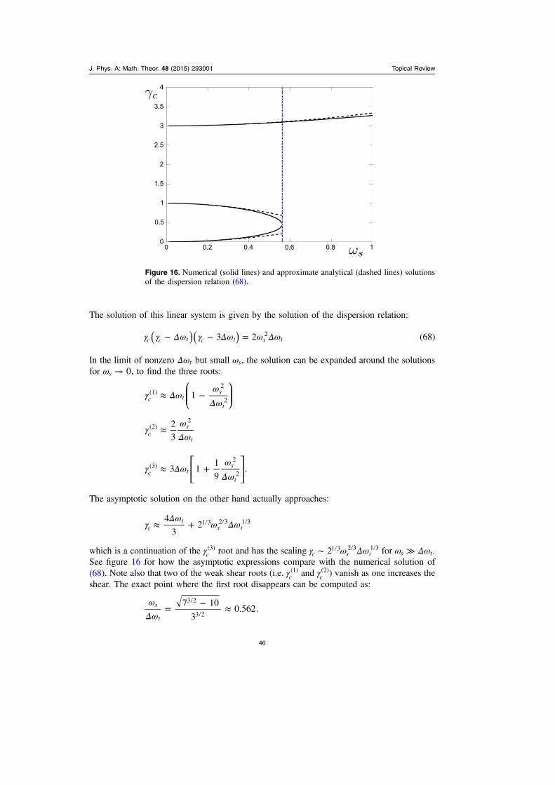
The solution of this linear system is given by the solution of the dispersion relation:

( )( )3 2 (68)c c t c t s t2γ γ Δω γ Δω ω Δω− − =

In the limit of nonzero tΔω but small sω , the solution can be expanded around the solutionsfor 0sω → , to find the three roots:

1c ts

t

(1)2

2γ Δω

ωΔω

≈ −⎛⎝⎜

⎞⎠⎟

2

3cs

t

(2)2

γωΔω

≈

3 11

9.c t

s

t

(3)2

2γ Δω

ωΔω

≈ +⎡⎣⎢

⎤⎦⎥

The asymptotic solution on the other hand actually approaches:

4

32c

ts t

1 3 2 3 1 3γΔω

ω Δω≈ +

which is a continuation of the c(3)γ root and has the scaling 2c s t

1 3 2 3 1 3γ ω Δω∼ for s tω Δω≫ .See figure 16 for how the asymptotic expressions compare with the numerical solution of(68). Note also that two of the weak shear roots (i.e. c

(1)γ and c(2)γ ) vanish as one increases the

shear. The exact point where the first root disappears can be computed as:

7 10

30.562.s

t

3 2

3 2

ωΔω

= − ≈

4

3.5

3

2.5

2

1.5

1

0.5

00 0.2 0.4 0.6 0.8 1

Figure 16. Numerical (solid lines) and approximate analytical (dashed lines) solutionsof the dispersion relation (68).


46

5.2. Effect on the resonance manifold

The resonance manifold, that defines how the wave-like fluctuations can interact with each-other efficiently is the key ingredient of the description of weak wave turbulence. A givenwave-number p interacts with two other wave-numbers q and k p q= − − (since theinteracting wavenumbers form a triangle). Thus, if p and p q− − are on the manifold definedby the Manley–Rowe relations p q p q( ) ( ) ( ) 0Δω ω ω ω≡ + + − − = (using the conventionthat frequency is taken as negative if the wavenumber is negative).

Consider for instance the resonance manifold given by the dispersion relation for theCharney–Hasegawa–Mima equation: ( )k k1k y

2ω = + :

( ) ( ) ( )p

p

q

q

p q

p qp q

q p( , )

1 1 1 2 ·0.

y y y y

2 2 2 2Δω ≡

++

+−

+

+ + +=

To consider the effect of constant shear, one can introduce the so-called shearing coordinates[83]:

t t x y v x t t( ), , ( ). (69)Ey0 0τ ξ η= − = = − ′ −

The other key element in computing the efficiency of three wave interactions is the interactioncoefficient. For the CHM system, it can be written as:

( )M

q p

k

z p qˆ ·

1.kpq

2 2

2=

× −

+The effect of a constant shear on the resonance manifold and the interaction coefficient can beseen in figure 17.

Figure 17. The resonant manifold p q k( ) ( ) ( ) 0Δω ω ω ω≡ + + ≈ , with q k p= − − ,in shearing coordinates as a function of time τ for p 0.6x = , p 0.4y = . The color codes

indicate the strength of the nonlinear interaction coefficient Mkpq. The figure shows thatwhile initially this mode was coupled to two other modes roughly k 1x ∼ − , k 0.3y ∼and k 0.6x ∼ , k 0.6y ∼ − , later on, both the size of the resonant manifold and the

nonlinear interaction coefficient on the resonant manifold diminish. This suggests thatthe three wave interactions become very ineffective.


47

It is well known that in plasmas and quasi-geostrophic fluids, weaknesses in resonantinteractions (i.e. that the manifold is small and the interaction coefficient vanishes on a largeportion of that manifold) is one of the primary reasons for the generation of large scale flowstructures. In other words, as the resonance manifold is weakened the only remaininginteraction that remains is via the large scale flow that satisfies the Manley–Rowe relations ina trivial way.

It is therefore interesting to see that the action of flow shear, indeed weakens the reso-nance manifold in time, hence a time averaged ‘effective’ resonant manifold also gets weaker.This leads to the turbulence being forced to couple even more to the large scale flow. In otherwords, while at the beginning of the shearing transformation the turbulence may have beencoupling to other modes, as the time increases, the eddies are tilted and they can only coupleto the large scale flow.

Physically this corresponds to tilting and absorption of small scale vortices by thesheared flow as discussed in [84]. This is a self-enhancing nonlinear mechanism that amplifiesthe initial shear as opposed to the vortex break up. This observation is interesting for control,because if we impose external flow shear, the same level of turbulence will generate morezonal flows under the action of large scale shear because the eddies can not couple to anythingelse other than the zonal flows due to the destruction of the resonance manifold. This meansthat for quasi-2D turbulence, by applying an external flow shear we can increase self gen-erated flow shear structures as well.

5.3. Self amplification

We have discussed various mechanisms by which a shear flow amplifies itself. First wediscussed the simple process of radial group velocity propagation of the waves that are tiltedin a certain direction giving rise to sheared flows which increase the tilt and hence theReynolds stress. Then there is the basic mechanism of modulational instability; a seed shearedflow which acts on fluctuations by modulating their amplitude results in ‘negative viscosity’and hence finite time singularity. Finally we discussed the effect of sheared flow on the three-wave interaction resonance manifold, noting that while initially the manifold is reasonablypopulated, as the sheared flow acts, the three wave interactions become less and less efficient,favoring the coupling with the zonal flows.

These are all different ways of describing a common phenomenon; that of the selfamplification of the zonal flow by its effect on turbulence. This usually corresponds to theinitial phase of the zonal flow growth and works until the fluctuations start to be seriouslymodified by the zonal shear that they are unable to sustain their energy.

6. PP dynamics

6.1. Basic PP dynamics

The fact that the zonal flow feeds on the energy of turbulent fluctuations, while suppressingthose same fluctuations that drive it, via shear decorrelation, suggests an analogy between thedynamics of the zonal flow/drift wave system and that of a predator and a prey species. In thisanalogy, the zonal flow acts as a predator, whose increased population becomes a threat to thedrift wave that play the role of the prey. The zonal flow damping is then a key controlparameter that determines, once the prey is gone, how long will the predators last. This is thekey parameter, along with the available free energy that sets the dynamics of the system. Thebasic Lotka–Volterra equations for zonal-flow drift-wave system can be obtained by


48

considering the zero-dimensional limit of the wave-kinetic formulation described insection 3.2:

N

tN E N N , (70)V

2γ α Δω∂∂

= − −

( )E

tNE E E E , (71)V

V F V nl V Vα ν γ∂∂

= − −

where N indicates the wave-quanta density and EV indicates the energy associated with zonalshear. Various coupling coefficients such as γ, the linear growth rate, α shearing efficiency,Δω, nonlinear decorrelation rate, Fν , the zonal flow damping and nlγ define the characteristicsof the model.

It is clear that the evolution of the turbulent fluctuations coupled to zonal flow energy asdescribed by the simplified model given by (70) and (71) describes the dynamics of a PPsystem. The prey species N has an internal growth as well as a nonlinear damping (due to‘eddy’ diffusion), while the predator species has linear damping but nonlinear growth -that isproportional to the population of the prey- as well as a higher order nonlinear damping (whichis not really necessary for a minimal model).

A PP cycle thus has four phases dominated subsequently by these four terms. It startswith the initial growth phase where the fluctuations grow exponentially. This is followed by apredation phase, where the zonal flows grow rapidly feeding off of the free energy of thefluctuations. This phase is characterized by modulational instability or self-enhanced growthof initially weak zonal perturbations. The next phase, characterized by shear suppression isthe phase where intense zonal flow shear scatters turbulence energy to high-k where it getsdissipated. In this phase the fluctuation intensity decreases. The final phase in the PP cycle isthe zonal flow damping phase. Physically this is usually the slowest phase, and therefore itdetermines the period of PP oscillations.

Figure 18. Temporal evolution of the Lotka–Volterra system (on the left) and its basicgeneralization that is used in plasma turbulence (on the right), where the fixed pointsgiven in (72) are shown as dashed lines. Here the variable x correspond to the primaryturbulence (prey) and the variable y corresponds to the zonal flow (the prey).


49

6.1.1. Lotka–Volterra. The basic Lotka–Volterra equations are given by

x

tax bxy

d

d= −

y

tcy dxy

d

d,= − +

where x correspond to drift waves (prey) and y to zonal flows (predator). The system has twofixed points for each variable given by x = 0, y = 0, x = c/d, y = a/b. The resulting oscillationis shown in figure 18.

6.1.2. The zonal flow variant. The equation

x

tax bxy ex

d

d2= − −

y

tcy dxy fy

d

d2= − + −

has the fixed points defined by

x a by ex( ) 0− − =

y c dx fy( ) 0− − + =which gives the nontrivial solution

xcb fa

db efy

a ec

b ef,

d

d(72)= +

+= −

+as we can see in figure 18, the system saturates by approaching this solution. While thedynamics of this simple model is representative of the similar dynamics in tokamaks, it is notclear if the fixed point remains meaningful even after considerable modeling effort to estimatethe coefficients. The model is actually a rather qualitative model that is used to developinsight into the tendencies rather than as a quantitative model.

6.2. PP and forward enstrophy cascade

When the zonal flows become important dynamically, low k drift wave spectrum is dominatedmainly by nonlocal interactions with the zonal flow. These interactions are anisotropic innature and are nonlocal in k-space in that the zonal shearing, can act on small scales directlyby transferring some of the PE in the drift waves (which is a conserved quantity of the zonalflow–drift wave interaction) to smaller scales.

However since the zonal flow obtains energy by transforming the PE of the low-k driftwave to the high-k one it becomes stronger, and as it becomes stronger it leads to more andmore spectral flux being dumped to small scales and dissipated. However as the zonal flowbecomes too effective in moving the PE to dissipation range, it starts to deplete its source.With some zonal flow damping, this leads to cycles of ‘bursts’ in the spectral evolutionequation of the zonal flow.

Consider for example the basic spectral budget for PE:

tW k

kq k

kk P k k( ) ( , ) ( ) ( ) ( ), (73)nℓ

WℓW

W WΠ Π ε∂∂

+ ∂∂

+ ∂∂

= −


50

where k( )ℓWΠ is the usual k-space flux of PE, driven by local interactions and q k( , )nℓΠ is the

part of the flux that is driven by nonlocal interaction with the zonal mode (of wave-number q).PW and Wε are the production and the dissipation of PE.

6.2.1. Spectrum with nonlocal interactions. Basic dimensional analysis suggests that

q k q k W k k( , ) ( , ) ( )nℓW

zf1Π τ= −

q k kE q q( , ) ( )zf1 1 2 1 2τ ∝−

now considering a constant nonlocal flux, we obtain:

W kk

u q( )

( ), (74)

2

rms

β=−

where u q E q q( ) ( )rms1 2 1 2= is the root mean square velocity of the zonal flow. Note that here

we took the zonal flow as a more general two-dimensional structure and considered theisotropized energy spectrum in order to preform a dimensional analysis. The basic scalingsshould work as long as there is an additional mechanism which isotropize the fluctuations atsmaller scales.

Remarkably, the spectrum

( )n

k

k1k k2 2

3

2 2Φ ∝ ∝

+

−

one obtains from (74) for ( )W k k k( ) 1k2 2 2

Φ∼ + (note that the extra k is an integrationfactor) seem to agree reasonably well with experimental observations of density fluctuationsin Tore Supra, especially for high-k where the turbulence is expected to be relativelyisotropic, using the Doppler back-scattering diagnostic system.

7. Role of zonal and mean flows in L–H transition

Recent observations of the intermediate phase (I-phase) that appear between L and H-modestates and display limit cycle oscillations between turbulence intensity and mean flows pointout the key role that the zonal flows play in the formation of transport barriers.

The basic role of E × B shear in H-mode is rather well understood. In a quasi-steady state,the energy injection rate + the energy generated by the fusion reactions (which is usuallyweak compared to the injected energy in current tokamaks, but will hopefully becomeimportant in the future ones) has to be balanced by the heat flux. However the heat transportin tokamaks is mainly turbulent, and since E × B shear reduces turbulence, and thus theturbulent diffusion coefficients, if a Fickʼs law is used to estimate the turbulent heat transportas the diffusion coefficient goes down, in order to keep the heat flux constant, the temperaturegradient has to go up. A similar argument can be made for the density. In fact there are anumber of simple transport models, which can ‘describe’ the L–H transition qualitativelyusing this basic idea [85].

7.1. Modeling the L–H transition.

The minimum model that can describe the L–H transition involves the E × B shear sup-pression mechanism where the E × B shear is somehow linked to either the temperaturegradient via the neoclassical expression for toroidal velocity [86], or density gradient times


51

temperature gradient via the radial force balance [85]. The minimal model, which has relevantphysics for the H-mode is a setup, somewhat related to a 1-D double diffusive convectionproblem encountered in the study of salinity transport in the ocean.

Consider a set of radial transport equations for density n r t( , ) and pressure P r t( , ):

[ ]tn

r rr S r

1( )n nΓ∂

∂+ ∂

∂=

tP

r rrQ H r

3

2

1[ ] ( ),p

∂∂

+ ∂∂

=

where a slow ‘transport time scale’ dynamics is assumed for the evolution of the profileswhich are averaged over the flux surfaces (in θ and ϕ directions around the torus), so thatfluctuations smooth out. It is further assumed that a basic closure for the heat and particlefluxes can be implemented such that:

Dn

rD

n

rn 0 1Γ = − ∂

∂− ∂

∂

QP

r

P

r,p 0 1χ χ= − ∂

∂− ∂

∂

where D0 and 0χ corresponds respectively to the residual part of the particle and heatdiffusivities usually thought to be due to neoclassical diffusion, and D1 and 1χ are theturbulent particle and heat diffusivities respectively, which are explicitly proportional to theturbulence intensity . A simple shear suppression rule in the spirit of section 5.1, whichcorrespond to the weak shear limit of reference [81], is usually used:

v1 Ey

02

α=

+ ′

to imitate the suppression of the turbulence due to sheared flow.Where usually an approximate form of the radial force balance for the ions:

Ev

cB

v

cB

P

enr = − + +θ

ϕϕ

θ

such as

vc

eBn

n

r

P

r

d

d

d

dEyi2

′ =

is used (recall that v cE BEy r= − ) [85]. The heat source H r( ) is localized in the center and theparticle source S r( ) is localized near the edge of the plasma. This system of equations solvedwith the boundary conditions n a n( ) a= , P a P( ) a= and n P(0) (0) 0t x t x∂ ∂ = ∂ ∂ = (andpossibly with other boundary conditions as well), gives a rather clear L–H transition (seefigure 19).

Many similar models have been developed, explaining the details of the bifurcationphenomenon [87], including angular momentum transport to explain intrinsic rotation[88, 89], including turbulence spreading [90] and turbulence-zonal flow PP evolution toexplain the L–I–H transition [90–92]. In our current understanding of the phenomenon, thezonal flows play an important role during the transition.


52

7.2. Models including PP dynamics

Recent observations of, slow coupled oscillations between plasma fluctuations and large scaleflow structures, display certain characteristics of PP dynamics. Such ‘limit cycle oscillations’have been observed in TJ-II stellerator [93], and HL-2A [94], ASDEX-Upgrade [95], D-IIID[96], EAST [97] and Alcator C-Mod [98] tokamaks and point to zonal flows as a universaltrigger to the L–H transition [99].

Figure 19. Dynamics and the final steady state of the basic transport model, showingthe establishment of the L-mode profiles (denoted with L) slightly below the criticalthreshold at q 2.9a = and the H-mode profiles (denoted with L) slightly above it at

q 3.0a = for pressure (on the left) and density (on the right). It is remarkable that the

L-mode profile is established very rapidly while the transition to H-mode takes time inthis formulation.

Figure 20. Limit cycle oscillations before an L–H transition as predicted by a simplemeso-scale model [100], the solid line corresponds to turbulence intensity, the dottedline to zonal flows and the dashed line corresponds to the mean flow (or equivalentlythe pressure gradient). Figure used with permission from Kim E-J and Diamond P H2003 Phys. Rev. Lett. 90 185006. Copyright 2003 American Physical Society.


53

http://dx.doi.org/10.1103/PhysRevLett.90.185006

While the experimental observations of the phenomenon are relatively new, the idea hasbeen around for a while. Most notably, Kim and Diamond had predicted the limit cycleoscillations [100] from a simple L–H transition model that includes zonal-flow turbulenceinteractions (see figure 20). The models have recently been extended in a series of papers byMiki and Diamond et al in the form of reduced meso-scale models of zonal flow triggering ofthe L–H transition [92, 101–103]. Similarly coupling a shell model of drift-wave turbulence(which incorporates naturally the PP evolution) to a transport model has given a qualitativelyconsistent picture of meso-scale evolution leading to pedestal formation [90].

The basic picture which arise from these theoretical studies and experimental observa-tions is that the zonal flows and therefore the meso-scale dynamics associated with them, suchas avalanches, turbulence spreading, spatial and spectral evolution of turbulence intensity intoregions of phase-space that are not linearly excited is an essential part of the dynamical self-regulation leading up to the L–H transition. Dominant paradigms based on a fixed back-ground gradient driving micro-turbulence, whose only effect is to define a turbulent diffusioncoefficient can not capture the PP behavior as a result of either the lack of or a strong dampingof mesoscale phenomenon. This suggests that a direct approach to modeling the turbulenttransport is more difficult than initially thought, since it requires a direct numerical simulationof the evolution of the full gyro-kinetic distribution function where the free energy sources arenot the gradients but rather explicit heating terms written in terms of fluxes. Such a ‘flux-driven’ simulation effort, has indeed been undertaken, but has shown to be rather difficultwith current resources, for realistic practical applications for tokamak plasmas [129].

This justifies the use of simpler models as discussed in this review, sometimes as the onlysource of prediction, as most direct numerical simulations are based on fixed imposed pro-files, which work only when the plasma is not dynamically evolving and basically has nohope of simulating a multi-scale dynamical phenomenon such as an L–I–H transition.

7.3. Staircases and sandpiles

PV staircases are a well known feature of the Earthʼs atmosphere related to zonal jets indifferent planets shown in figures 1 and 2 in section 1. They are also a key feature of thethermohaline, and provide a barrier for the thermal transport across different layers of theocean. They also probably exist in tokamaks and act as a seed for the formation of the actualtransport barrier.

While staircases reduce transport across them due to the flow shear associated with them,they don’t completely suppress turbulence. As a result the flux that is slightly reduced leads toan accumulation of the transported quantity leading to a sharpening of its gradient and hencethe possibility of a sudden burst of transport. This dynamical coupling between a formingstaircase pattern and a sudden burst of transport (an ‘avalanche’) is a secondary meso-scaledynamics of plasma turbulence that has important implications on the dynamics of the profiles(i.e. transport) especially formation and destruction of barriers.

An interesting aspect of avalanche dynamics is its relation to self organized criticality(SOC) and thus sandpiles. One may intuitively expect that the plasma when driven far fromequilibrium drives sheared flows and other complex mesoscale structures to bring itself near aself-organized critical ‘equilibrium’. In this dynamical state, the plasma would be in a state oflocally marginal equilibrium hovering slightly above and slightly below this self-organizedmarginal stability curve.

Leaving the question of what this marginal equilibrium is and how it is established aside,we may describe the evolution of the profiles around this equilibrium. Noting that the jointreflection symmetry x x→ − , P Pδ δ→ − is respected [104] by the flux near an SOC


54

equilibrium state (such that P P PSOC δ= + ), one can consider a combination of the simplestpossible forms of the flux as p P P( ) ( 2)

x2Γ δ λ δ χ δ≈ − ∂

∂. This gives the following equation

for the deviation from the SOC state for the plasma pressure [105]:

tP

xP

x xP

202δ λ δ χ δ∂

∂+ ∂

∂− ∂

∂∂∂

=⎜ ⎟ ⎜ ⎟⎛⎝

⎞⎠

⎛⎝

⎞⎠

which can be recognized as the Burgers equation. Since the Burgerʼs equation leads toformation of shocks, and a slower process of PV homogenization counters this tendency, it isnot surprising that the system generates ‘staircase’ patterns.

The effect of a mean sheared flow on this basic Burgers dynamics can be included byadding another direction to consider a flow in the y direction that is sheared in the x direction.This gives a ‘transport’ equation of the form:

tP v x

yP

xP

x xP

y yP

20E

2δ δ λ δ χ δ χ δ∂∂

+ ′ ∂∂

+ ∂∂

− ∂∂

∂∂

− ∂∂

∂∂

=⎜ ⎟ ⎜ ⎟⎛⎝

⎞⎠

⎛⎝

⎞⎠

⎛⎝⎜

⎞⎠⎟

which is still consistent with the joint reflection symmetry.

8. Nonlocality, radial propagation

Another mechanism by which the zonal flow/drift wave system can saturate is through spatialpropagation. We have already seen a glimpse of that in the modulational instability frame-work as we made a transformation to the frame of reference, moving radially at the radialgroup velocity. The zonal flow, which does not move is then retarded in this reference frameand it is this effect that balances the Reynolds stress at the lowest order. However in realitythe coupling of spatial propagation and zonal flows is not as simple. Since modulations thatare generated in different spatial positions with different characteristics and can propagateeither inward or outward both due to linear and nonlinear effects.

In nature, turbulence is never local. If a local perturbation injects energy to a turbulentfield locally in space, the resulting fluctuations spread throughout the system. The phenom-enon while obvious from a turbulence perspective, may appear counter-intuitive from amagnetized plasma perspective where the particles are well localized due to small Larmorradii.

However since turbulent transport allow the particles or heat to be transported radiallydue to phase relations of fluctuating fields, the generated turbulence can also propagate viathese same turbulent mechanisms. The phenomenon that is called ‘turbulence spreading’ isusually described using Fokker–Planck formulations resulting in Fischer–Kolmogorov typenonlinear equations, such as:

t xv D

x, (75)g nℓ0

2 γ γ∂∂

+ ∂∂

− ∂∂

= −⎡⎣⎢

⎤⎦⎥

where x t( , ) is a measure of the turbulent fluctuation level (usually a nonlinearly conservedquantity such as energy, or PE).

The equation can also be obtained by a systematic reductive perturbation method basedon the two scale direct interaction approximation, which is applicable to two and more fieldmodels of turbulence [106]. The equation (75) has a number of exact solutions for certainforms of γ and nℓγ that are physically relevant solutions, such as self-similar spreading orballistic fronts [107].


55

A detailed derivation of a similar equation can be done, starting from the drift-kineticequation, where the flux can be written as an integral over the velocity space of the flux offree-energy density, instead of the particular form (i.e. v Dg x0 Γ = − ∂

∂ ) that was takenabove:

f

f

f

fv d v

vb

2 2ˆ , (76)

E2 2

3 ∫Γ ≡ +∼ ∼ ∼

∥

⎛

⎝

⎜⎜⎜

⎞

⎠

⎟⎟⎟

where f and f∼being the slowly evolving and the rapidly fluctuating parts of the drift kinetic

distribution function.Basic effect of large scale flow shear can be included in this equation by including the

physics of advection by a radially sheared poloidal flow:

tv x

y xv D

x.E g nℓ0

2 γ γ∂∂

+ ′ ∂∂

+ ∂∂

− ∂∂

= −⎡⎣⎢

⎤⎦⎥

A formulation of this form is not self consistent unless one includes the effect of fluctuationson driving the E × B shear. It may however be useful in the case, when the E × B shear issufficiently strong and steady that it can be considered as an external one. The H-mode intokamaks would satisfy this condition.

However for the transition, current understanding suggests that the spatio-temporal PPlike dynamics of turbulent fluctuations and zonal flows with mean E × B shear acting as areservoir of kinetic energy play the dominant role. While the fluctuations can recover fromzonal shear suppression due to zonal flow damping, mean shear eventually acquires enoughenergy and suppresses the turbulent fluctuations sufficiently, reducing the transport coeffi-cients considerably leading to a state of high confinement.

It should be noted however that the simple PP idea described above, which will bediscussed in more detail below, does not take into account the spatial propagation. None-theless, both the fluctuations and the zonal flows actually propagate as they are nonlinearlycoupled forming complex interaction patterns. A description of this phenomenon usingsimple models is possible and interesting in its own right. However even the simplest modelends up with 4-5 partial differential equations describing spatio-temporal evolution of dif-ferent quantities.

8.1. Telegraph equation, traffic flow, and turbulent elasticity

8.1.1. Telegraph equation. In the standard formulation of plasma transport, the response ofthe flux to the gradient is usually taken to be local and instantaneous There is a direct relationbetween the heat flux and the temperature gradient (i.e. with adiabatic electrons and zerorotation with symmetric k∥ spectrum):

QT

r. (77)iχ= − ∂

∂

This relation is called the Fickʼs law (or the Fourier law of heat conduction in the case ofsolids), and it implies that the flux responds infinitely rapidly and perfectly locally to thegradients. In contrast, ‘the second sound’ [108], in solids at very fast time scales [109], and inreactive fluids, a commonly used relation is the following (e.g. [110]):


56

Q

tT Q 0, (78)i rτ χ∂

∂+ + =

where τ can be considered as a new coefficient of transport physics, which physicallycorresponds to the response time of the flux to the gradient. This relation, which is called theMaxwell–Cattaneo relation, incorporates the fact that if the gradient is suddenly changed, theheat flux would respond in some finite response time (i.e. τ). Notice that, the steady state limitof (78) is indeed (77). In order to understand ‘transient’ transport, we actually need both τ and

iχ even though τ may be as fast as a few turbulent decorrelation times.However since the plasma transport is driven mainly by turbulence, the response of the

flux is not a simple ‘transient’, because by the time the flux is saturated to its mixing lengthlevel, the gradient is also changed via the transport equation for heat:

T

tQ H r t· ( , ), (79)i

r i∂∂

+ =

where H r t( , ) is the net heating, and this allows a dynamical coupling between the flux andthe gradient. For example expanding around an equilibrium (i.e. Q H r t· ( , )r i = ), it is easyto see that the excess temperature obeys the equation:

T

t tT T

1· 0 (80)i

i ri

r

2

2

δτ

δχτ

δ∂∂

+ ∂∂

− = ⎡⎣⎢

⎤⎦⎥

which is actually the telegraph equation. This equation is well known to describe the timeevolution of the transport in reactive fluids and in problems of population growth, moreaccurately than a simple diffusion equation [111, 112]. It is the simplest formulation thatdescribes the phenomenon of diffusion in a medium, which describes not only the positions,but also the momenta of the basic elements [113] that constitute that medium. It is clear thatas 0τ → , the first term in (80) becomes negligible and we recover the usual diffusionequation. Note that this is a singular limit where the highest order derivative with respect totime drops.

In contrast, for finite τ, the wave character of the equation suggests a radial propagationspeed vr iχ τ= , which is consistent with the spreading phenomenology v D2spr γ∼(where γ is the growth rate), except that the diffusion coefficient for turbulence intensity D isreplaced in this coupled formulation by the heat diffusivity iχ [107, 114–116].

If the flux response is not perfectly local, but rather smoothed out (i.e. a discontinuity inthe gradients, does not generate a step function flux), we can write:

Q

tT Q 0, (81)r Q i rτ τ Γ χ∂

∂+ + + =

where a local closure for the flux of heat flux:

DQ

r(82)QΓ = − ∂

∂

can be proposed, which gives the so-called Guyer–Krumhansl constitutive relation [117],which is sometimes referred to as a ‘weakly nonlocal’ relation. Obviously, if the radial groupvelocity of the waves that are responsible for transport is finite, it should be added to QΓ (i.e.as v Qgr ).

Note that this formulation of the transport now has three coefficients, namely the heatdiffusivity iχ , flux response time τ and the flux penetration length Dλ τ= . Note that (81) issimply the Cattaneo relation with the added diffusion of heat flux. However since, the


57

transport is anomalous in fusion plasmas, the coefficients ,χ τ and D are functions ofturbulence intensity, rendering the constitutive relation nonlinear as will be discussed.

The effect of mean shear can be introduced into the equation for the heat flux by movingto two dimensions as:

tv x

yQ T Q 0.E r Q i rτ τ Γ χ∂

∂+ ′ ∂

∂+ + + =

⎛⎝⎜

⎞⎠⎟

8.1.2. Turbulent elasticity and PP waves. The basic approach that has been outlined in theprevious section for weakly nonlocal evolution of the heat flux can be applied to otherquantities that are transported in a plasma, such as particles and momentum. A full matrixformulation is discussed in appendix B as a starting point for this generalization. Howeversince such a formulation is by definition ‘meso-scale’ both in time and in space, other meso-scale phenomena, and in particular zonal flows has to be included in the same footing. Whilethe zonal flows are special in the sense that they suppress the underlying turbulence, they aredriven by a perpendicular momentum flux, just as any other flow can be driven by momentumflux. In fact the zonal momentum flux evolution can be obtained simply by taking thecorresponding moment of the wave-kinetic equation. Following [118], we consider the wavekinetic equation (33), which can be written as:

( )tN v

xN k v

kN N N (83)k g k k y E k N k k k, , 0,γ∂

∂+ ∂

∂− ′ ∂

∂= − −

coupled to the spatio-temporal evolution of the zonal+mean flow:

( )tv

xv v .E y F E E,0Π ν∂

∂+ ∂

∂= − −

The wave-quanta density Nk is driven towards N k0, , which is the steady state k-spectrum dueto eddy damping, and vE, which is the zonal E × B velocity is driven towards vE,0 -the E × Bflow implied by the radial force balance- due to ZF damping mechanisms discussed above.Here

v vy x yΠ = ∼ ∼

is the radial flux of zonal momentum and using the equivalence of wave-particle momenta[79] is equivalent to wave-momentum, which can be computed by multiplying (83) by v kg k y,

and integrating over k as:

( )t x x

v . (84)y

y E N y y0

ΠΓ α γ Π Π

∂∂

+ ∂∂

+ ∂∂

= − −Π

Here Nγ is the expectation value of N k,γ over the ‘distribution’ N N Nk k k0,δ = − . The local,steady-state limit of (84), gives a Fickʼs law like expression for the zonal flow:

xv ,y y

NE0Π Π α

γ= − ∂

∂

where y0Π plays the role of a residual momentum flux [89, 119] in the absence of E × B shear.

One can get a simple telegraph equation for the zonal flow, even by dropping thex yΓΠ

∂∂

termaltogether (i.e. considering a delayed response, but no spatial coupling).


58

t xv

yE N y

Πα γ Π

∂∂

+ ∂∂

= −∼

tv

xv ,E y F EΠ ν∂

∂+ ∂

∂= −∼ ∼

where y y y0Π Π Π= − and v v vE E E0= −∼ are the meso-scale time evolving components. Thetwo equations can be combined simply as:

t tv

xv 0F N E E

2

2ν γ α∂

∂+ ∂

∂+ − ∂

∂=∼ ∼⎜ ⎟⎜ ⎟⎛

⎝⎞⎠

⎛⎝

⎞⎠

which suggest damped wave-like solutions independent of the sign and the value of α. Thismeans that in order to excite spatial PP waves, one has to include some form of spatialnonlocality.

Since we are not interested in the temporal evolution of yΓΠ , we can use a flux-limiteddiffusion [120, 121] expression as a ‘closure’:

( )x

1 lny

y y

y x y2

Γχ Π

λ Π= −

∂∂

+Π

Π

Π∂∂

for 0yλ →Π or lnx y y

1 2Π λ≪ Π∂∂

− , the expression gives the usual Fickʼs law, but in theopposite limit it gives advection. In this latter limit, the combined equation takes the form of ageneralized telegraph equation:

t tv

x xv 0. (85)F N c E

2

2ν γ α∂

∂+ ∂

∂+ − ∂

∂− ∂

∂=∼⎜ ⎟⎜ ⎟

⎡⎣⎢

⎛⎝

⎞⎠

⎛⎝

⎞⎠

⎤⎦⎥

The modulational instability condition for (85) is q N F2α γ ν> , which also gives a critical

(i.e. most unstable) zonal wave-number as qc F N1 2ν γ α≈ . It is clear that once these radially

propagating PP waves establishes, all the fluxes become equally nonlocal, since the localgradients of temperature, density and momentum, will all be determined by the incomingfluxes via this dynamics rather than the other way around.

With this we may be able to say a few words about a current debate in the fusioncommunity about fixed gradient versus flux driven formulations. It is true that the turbulencein fusion devices are excited locally by the free energy in the gradients. However aformulation based on fixed gradients is not very meaningful since the profiles themselvesadjust in order to be able to accommodate the injected heat, particles and momentum. Thismeans that a flux-driven formulation (source-driven is usually implied) is critical fordescribing the evolution of the plasma globally. However a global description necessitates aproper implementation of boundary conditions and different parts of the plasma, such as openand closed field lines. Instead a partially local description can be imagined where the fluxesand the gradients co-evolve in the domain, and the boundary conditions are chosen as thefluxes and the gradients at the boundary of the domain. If the simulated domain does notcontain sources, such a partially local formulation may be sufficient for describing the weaklynonlocal dynamics of the plasma turbulence.


59

Acknowledgments

This research was supported in part by the National Science Foundation under Grant No. NSFPHY11-25915.

Appendix A. Derivation of thermal Rossby equations

Considering a viscous fluid in the container depicted in figure 3, the equation of motion canbe written as:

t

Pv v n v r v· 2 ˆ . (A.1)2 2Ω Ω

ρν∂

∂+ + × + = − +

⎜ ⎟⎛

⎝⎞⎠

Using a perturbation expansion, P P P0 δ= + , and 0ρ ρ δρ= + , the zeroth order balancewith no flow takes the form

P r r. (A.2)0 02

0ρ Ω= −

When we substitute these expansions back into (A.1), and use (A.2) to eliminate P0 , weobtain:

t

Prv v n v r v· 2 ˆ ˆ . (A.3)

0

20

0

2Ω δρ

Ω δρρ

ν∂∂

+ + × = − − +

⎜ ⎟⎛⎝

⎞⎠

Using the equation of state:

( )T T10 0ρ ρ α= − −⎡⎣ ⎤⎦we can write T0δρ αρ δ= − where Tδ is the deviation from an equilibrium profile oftemperature, which is the steady state solution of the heat equation:

tT Tv · (A.4)2κ∂

∂+ = ⎜ ⎟⎛

⎝⎞⎠

which actually becomes the Laplaceʼs equation T 020 = , one solution to which is a constant

gradient linking the two boundary values of temperature

T x TT

Dx( ) . (A.5)0 1

Δ= +

Multiplying (A.3) by D3 2ν , and using the dimensionless variables Dv v ν′ = , t t D2ν′ = ,

Dx x′ = , D P2

20

π =ν

δρ and T T( )Θ δ Δ= :

tE Rav v n v r v· 2 ˆ ˆ , (A.6)1 2π Θ∂

∂+ + × = − + +− ⎜ ⎟⎛

⎝⎞⎠

where we dropped the primes for convenience and defined

RaD T

r ,3

20α Δ

νκΩ≡

which is the Rayleigh number, and

ED

,2

νΩ

≡

which is the Ekman number. The equation for temperature perturbation can be obtained bysubstituting T T x T( )0 δ= + with T x( )0 given by (A.5) into the heat equation (A.4):


60

tT v

T

DTv · x

2δ Δ κ δ∂∂

+ + = ⎜ ⎟⎛⎝

⎞⎠

multiplying by D T( )2 νΔ and using the normalization discussed above, we obtain:

tvv · . (A.7)x

2 Θ Θ∂∂

+ + = ⎜ ⎟⎛⎝

⎞⎠

Using v n ψ= × ⊥ , and the geostrophic balance as described already in section 1.2.3 thesystem of equations (A.6) and (A.7) can be written as

( )( )t

E Ray

v v· 2 ·1 2ζ ζ Θ ζ∂∂

+ + + = − ∂∂

+−⊥ ⎜ ⎟⎛

⎝⎞⎠

using (3) with h h x h x( ) 20 0η= = − , we can write

tRa

yv · * ,y

2ζ η ψ Θ ζ∂∂

+ − ∂ = − ∂∂

+ ⎜ ⎟⎛⎝

⎞⎠

where ( )Eh* 4 0 0η η= .

Appendix B. Matrix formulation of weakly nonlocal transport

One can formulate general transport equations with evolving fluxes in simple geometry asfollows:

tS· (B.8)rξ Γ∂

∂+ =

( )t

· [ · ] · , (B.9)rres Γ Γ Γτ ∂∂

+ − + = R M

where

nnTnv

Q,n

ξ ΓΓ

Π= =

ϕ ϕ

⎛⎝⎜⎜

⎞⎠⎟⎟

⎛

⎝⎜⎜⎜

⎞

⎠⎟⎟⎟

nT

v

D U U

U U

U U,

r

r

n nT n

Tn i T

n T

χχ

= = −ϕ

ϕ

ϕ

ϕ ϕ ϕ

M

⎛

⎝⎜⎜⎜

⎞

⎠⎟⎟⎟

⎛

⎝

⎜⎜⎜

⎞

⎠

⎟⎟⎟

Q

D U U

U D U

U U D

, .r n

r

r

Q

Q Q Q

Q

n n n

n

n

Γ

Π= = −

ϕ

Γ Γ Γ Π

Γ Π

Π Γ Π Π

ϕ

ϕ

ϕ ϕ ϕ

R

⎛

⎝⎜⎜⎜

⎞

⎠⎟⎟⎟

⎛

⎝

⎜⎜⎜⎜

⎞

⎠

⎟⎟⎟⎟

Furthermore these can be extended to include temperature anisotropy as well as magneticcurvature and inhomogeneity separating turbulent and neoclassical contributions to the flux[122]. Note that in the above formulation the neoclassical fluxes should appear as offset, notas a modification of the fixed point. In other words, we would say neo turbΓ Γ Γ= + and write(B.9) only for the turbulent bit. Here we present this matrix formulation as the basis of analternative to standard transport frameworks (e.g. [123]).


61

References

[1] Rhines P B and Young W R 1982 J. Fluid Mech. 122 347–67[2] Larichev V and Reznik G 1976 Dokl. Akad. Nauk SSSR 231 1077–9[3] Flierl G R, Stern M E and Jr J A W 1983 Dyn. Atmos. Oceans 7 233–63[4] Meiss J D and Horton W 1983 Phys. Fluids 26 990–7[5] Taylor J B 1974 Phys. Rev. Lett. 33 1139–41[6] Diamond P H and Malkov M 2003 Phys. Plasmas (1994–present) 10 2322–9[7] Dobrowolny M, Mangeney A and Veltri P 1980 Phys. Rev. Lett. 45 144–7[8] Grappin R, Frisch U, Pouquet A and Leorat J 1982 Astron. Astrophys. 105 6–14[9] Boldyrev S 2006 Phys. Rev. Lett. 96 115002[10] Levin S A 1998 Ecosystems 1 431–6[11] Frisch U 1995 Turbulence: The Legacy of A N Kolmogorov (Cambridge: Cambridge University

Press)[12] Ingersoll A P, Beebe R F, Collins S A, Hunt G E, Mitchell J L, Muller P, Smith B A and

Terrile R J 1979 Nature 280 773–5[13] Maximenko N A, Bang B and Sasaki H 2005 Geophys. Res. Lett. 32 L12607[14] Fujisawa A 2009 Nucl. Fusion 49 013001[15] Lin Z, Hahm T S, Lee W W, Tang W M and White R B 1998 Science 281 1835–7[16] Brizard A 1992 Phys. Fluids B 4 1213–28[17] Hockey T A 1999 Galileoʼs Planet : Observing Jupiter Before Photography (Bristol: Institute of

Physics)[18] Porco C C et al 2003 Science 299 1541–7[19] García-Melendo E, Pérez-Hoyos S, Sánchez-Lavega A and Hueso R 2011 Icarus 215 62–74[20] Peek B M 1958 The Planet Jupiter (London: Faber and Faber) http://archive.org/details/

ThePlanetJupiter[21] García-Melendo E and Sánchez-Lavega A 2001 Icarus 152 316–30[22] NASA/JPL/University of Arizona 2000 PIA02863: Planetwide Color Movie http://photojournal.

jpl.nasa.gov/catalog/PIA02863[23] Maximenko N A, Melnichenko O V, Niiler P P and Sasaki H 2008 Geophys. Res. Lett. 35

L08603[24] Richards K J, Maximenko N A, Bryan F O and Sasaki H 2006 Geophys. Res. Lett. 33 L03605[25] Rossby C G 1940 Q. J. R. Meteorol. Soc. 66 68–87[26] Vallis G K 2006 Atmospheric and Oceanic Fluid Dynamics: Fundamentals and Large-scale

Circulation 1st edn (Cambridge, UK: Cambridge University Press)[27] Pedlosky J 1987 Geophysical Fluid Dynamics 2nd edn (New York: Springer)[28] Hoskins B J, McIntyre M E and Robertson A W 1985 Q. J. R. Meteorol. Soc. 111 877–946[29] Fultz D and Nakagawa Y 1955 Proc. R. Soc. A 231 211–25[30] Hide R 1958 Phil. Trans. R. Soc. A 250 441–78[31] Chandrasekhar S 1953 Proc. R. Soc. A 217 306–27[32] Read P L, Yamazaki Y H, Lewis S R, Williams P D, Miki-Yamazaki K, Sommeria J,

Didelle H and Fincham A 2004 Geophys. Res. Lett. 31 L22701[33] Busse F H 2004 Chaos 14 803[34] Busse F H and Or A C 1986 J. Fluid Mech. 166 173–87[35] Chandrasekhar S 1961 Hydrodynamic and Hydromagnetic Stability (Dover Classics of Science

and Mathematics) (New York: Dover)[36] Diamond P H, Itoh S-I, Itoh K and Hahm T S 2005 Plasma Phys. Control. Fusion 47 R35–161[37] McKee G R et al 2003 Phys. Plasmas 10 1712–9[38] Tynan G R, Moyer R A, Burin M J and Holland C 2001 Phys. Plasmas 8 2691–9[39] Moyer R A, Tynan G R, Holland C and Burin M J 2001 Phys. Rev. Lett. 87 135001[40] Xu G S, Wan B N, Song M and Li J 2003 Phys. Rev. Lett. 91 125001[41] Fujisawa A, Itoh K, Iguchi H et al 2004 Phys. Rev. Lett. 93 165002[42] Estrada T et al 2009 Plasma Phys. Control. Fusion 51 124015[43] Manz P, Ramisch M and Stroth U 2009 Phys. Rev. Lett. 103 165004[44] Tynan G R et al 2006 Plasma Phys. Control. Fusion 48 S51[45] Sokolov V, Wei X, Sen A K and Avinash K 2006 Plasma Phys. Control. Fusion 48 S111[46] Fujisawa A, Itoh K, Shimizu A et al 2008 Phys. Plasmas 15 055906[47] Jakubowski M, Fonck R J and McKee G R 2002 Phys. Rev. Lett. 89 265003


62

http://dx.doi.org/10.1017/S0022112082002250

http://dx.doi.org/10.1017/S0022112082002250

http://dx.doi.org/10.1017/S0022112082002250

http://dx.doi.org/10.1016/0377-0265(83)90007-6

http://dx.doi.org/10.1016/0377-0265(83)90007-6

http://dx.doi.org/10.1016/0377-0265(83)90007-6

http://dx.doi.org/10.1063/1.864251

http://dx.doi.org/10.1063/1.864251

http://dx.doi.org/10.1063/1.864251




http://dx.doi.org/10.1063/1.1576390

http://dx.doi.org/10.1063/1.1576390

http://dx.doi.org/10.1063/1.1576390





http://dx.doi.org/10.1007/s100219900037

http://dx.doi.org/10.1007/s100219900037

http://dx.doi.org/10.1007/s100219900037

http://dx.doi.org/10.1038/280773a0

http://dx.doi.org/10.1038/280773a0

http://dx.doi.org/10.1038/280773a0

http://dx.doi.org/10.1029/2005GL022728

http://dx.doi.org/10.1088/0029-5515/49/1/013001

http://dx.doi.org/10.1126/science.281.5384.1835



http://dx.doi.org/10.1063/1.860129

http://dx.doi.org/10.1063/1.860129

http://dx.doi.org/10.1063/1.860129

http://dx.doi.org/10.1126/science.1079462



http://dx.doi.org/10.1016/j.icarus.2011.07.005



http://archive.org/details/ThePlanetJupiter

http://archive.org/details/ThePlanetJupiter

http://dx.doi.org/10.1006/icar.2001.6646



http://photojournal.jpl.nasa.gov/catalog/PIA02863

http://photojournal.jpl.nasa.gov/catalog/PIA02863

http://dx.doi.org/10.1029/2008GL033267

http://dx.doi.org/10.1029/2008GL033267

http://dx.doi.org/10.1029/2005GL024645

http://dx.doi.org/10.1002/qj.49711147002

http://dx.doi.org/10.1002/qj.49711147002

http://dx.doi.org/10.1002/qj.49711147002

http://dx.doi.org/10.1098/rspa.1955.0167



http://dx.doi.org/10.1098/rsta.1958.0004






http://dx.doi.org/10.1029/2004GL020106

http://dx.doi.org/10.1063/1.1774413

http://dx.doi.org/10.1017/S0022112086000095

http://dx.doi.org/10.1017/S0022112086000095

http://dx.doi.org/10.1017/S0022112086000095

http://dx.doi.org/10.1088/0741-3335/47/5/R01

http://dx.doi.org/10.1088/0741-3335/47/5/R01

http://dx.doi.org/10.1088/0741-3335/47/5/R01

http://dx.doi.org/10.1063/1.1559974

http://dx.doi.org/10.1063/1.1559974

http://dx.doi.org/10.1063/1.1559974

http://dx.doi.org/10.1063/1.1357220

http://dx.doi.org/10.1063/1.1357220

http://dx.doi.org/10.1063/1.1357220




http://dx.doi.org/10.1088/0741-3335/51/12/124015


http://dx.doi.org/10.1088/0741-3335/48/4/S05

http://dx.doi.org/10.1088/0741-3335/48/4/S08

http://dx.doi.org/10.1063/1.2889012


[48] Schmitz L, Wang G, Hillesheim J C, Rhodes T L, Peebles W A, White A, Zeng L, Carter T A andSolomon W 2008 Rev. Sci. Instrum. 79 10F113

[49] Hamada Y, Nishizawa A, Ido T, Watari T, Kojima M, Kawasumi Y, Narihara K, Toi K andGroup J I 2005 Nucl. Fusion 45 81

[50] Conway G D, Scott B, Schirmer J, Reich M, Kendl A and the ASDEX Upgrade Team 2005Plasma Phys. Control. Fusion 47 1165

[51] Nagashima Y et al 2005 Phys. Rev. Lett. 95 095002[52] Vershkov V, Shelukhin D, Soldatov S, Urazbaev A, Grashin S, Eliseev L, Melnikov A and

the T-10 team 2005 Nucl. Fusion 45 S203[53] Zhao K J et al 2006 Phys. Rev. Lett. 96 255004[54] Vermare L, Hennequin P, Gürcan Ö D and the Tore Supra Team 2012 Nucl. Fusion 52 063008[55] Yu J, Holland C, Tynan G, Antar G and Yan Z 2007 J. Nucl. Mater. 363–5 728–32[56] Jackson J D 1998 Classical Electrodynamics Third Edition 3rd edn (New York: Wiley) ISBN

047130932X[57] Yoshida Z and Mahajan S M 2002 Phys. Rev. Lett. 88 095001[58] Meyrand R and Galtier S 2012 Phys. Rev. Lett. 109 194501[59] Chew G F, Goldberger M L and Low F E 1956 Proc. R. Soc. A 236 112–8[60] Hasegawa A and Wakatani M 1983 Phys. Rev. Lett. 50 682–6[61] Horton W 1999 Rev. Mod. Phys 71 735–78[62] Vallis G K and Maltrud M E 1993 J. Phys. Oceanogr. 23 1346–62[63] Balescu R 2005 Aspects of Anomalous Transport Plasmas (Series in Plasma Physics) (Bristol:

Institute of Physics)[64] Goldreich P and Sridhar S 1995 Astrophys. J. 438 763–75[65] Carnevale G F and Martin P C 1982 Geophys. Astrophys. Fluid Dyn. 20 131–64[66] Dubrulle B and Nazarenko S 1997 Physica D 110 123–38[67] Smolyakov A I and Diamond P H 1999 Phys. Plasmas 6 4410–3[68] Balescu R 2003 Phys. Rev. E 68 046409[69] Balescu R, Petrisor I and Negrea M 2005 Plasma Phys. Control. Fusion 47 2145[70] Krommes J A and Kim C B 2000 Phys. Rev E 62 8508–39[71] Zakharov V E and Kuznetsov E A 1997 Phys. Usp. 40 1087[72] Falkovich G 2011 Fluid Mechanics: A Short Course for Physicists 1st edn (Cambridge:

Cambridge University Press)[73] Newell A 1974a Nonlinear Wave Motion (Lectures in Applied Mathematics) (Providence, RI:

American Mathematical Society) p 15[74] Kim E j, Holland C and Diamond P H 2003 Phys. Rev. Lett. 91 075003[75] Manfroi A J and Young W R 1999 J. Atmos. Sci. 56 784–800[76] Dimits A M et al 2000 Phys. Plasmas 7 969–83[77] Terry P W, Gatto R and Baver D A 2002 Phys. Rev. Lett. 89 205001[78] Itoh K, Hallatschek K, Toda S, Sanuki H and Itoh S I 2004 J. Phys. Soc. Japan 73 2921–3[79] Diamond P H, Gurcan O D, Hahm T S, Miki K, Kosuga Y and Garbet X 2008 Plasma Phys.

Control. Fusion 50 124018[80] Diamond P H, Liang Y M, Carreras B A and Terry P W 1994 Phys. Rev. Lett. 72 2565–8[81] Biglari H, Diamond P H and Terry P W 1990 Phys. Fluids B 2 1–4[82] Terry P W 2000 Rev. Mod. Phys. 72 109–65[83] Goldreich P and Lynden-Bell D 1965 Mon. Not. R. Astron. Soc. 130 125[84] Manz P, Ramisch M and Stroth U 2009 Phys. Rev. Lett. 103 165004[85] Hinton F L and Staebler G M 1993 Phys. Fluids B 5 1281–8[86] Hinton F L 1991 Phys. Fluids B 3 696–704[87] Malkov M A and Diamond P H 2008 Phys. Plasmas 15 122301[88] Dominguez R R and Staebler G M 1993 Phys. Fluids B 5 3876–86[89] Gürcan Ö D, Diamond P H, Hahm T S and Singh R 2007 Phys. Plasmas 14 042306[90] Berionni V 2014 Etude de l’impact des flux zonaux sur la turbulence plasma, la transition LH et

la production d’entropie PhD Thesis LPP, Ecole Polytechnique in preparation[91] Kim E and Diamond P 2003 Phys. Plasmas 10 1698–704[92] Miki K, Diamond P H, Gürcan Ö D, Tynan G R, Estrada T, Schmitz L and Xu G S 2012 Phys.

Plasmas 19 092306[93] Estrada T, Happel T, Hidalgo C, Ascasibar E and Blanco E 2010 Europhys. Lett. 92 35001[94] Zhao K J et al 2010 Plasma Phys. Control. Fusion 52 124008


63

http://dx.doi.org/10.1063/1.2953675

http://dx.doi.org/10.1088/0029-5515/45/2/002

http://dx.doi.org/10.1088/0741-3335/47/8/003


http://dx.doi.org/10.1088/0029-5515/45/10/S17


http://dx.doi.org/10.1088/0029-5515/52/6/063008

http://dx.doi.org/10.1016/j.jnucmat.2007.01.253













http://dx.doi.org/10.1103/RevModPhys.71.735



http://dx.doi.org/10.1175/1520-0485(1993)023<1346:GOMFAJ>2.0.CO;2



http://dx.doi.org/10.1086/175121

http://dx.doi.org/10.1086/175121

http://dx.doi.org/10.1086/175121

http://dx.doi.org/10.1080/03091928208209002

http://dx.doi.org/10.1080/03091928208209002

http://dx.doi.org/10.1080/03091928208209002

http://dx.doi.org/10.1016/S0167-2789(97)00120-6

http://dx.doi.org/10.1016/S0167-2789(97)00120-6

http://dx.doi.org/10.1016/S0167-2789(97)00120-6

http://dx.doi.org/10.1063/1.873725

http://dx.doi.org/10.1063/1.873725

http://dx.doi.org/10.1063/1.873725

http://dx.doi.org/10.1103/PhysRevE.68.046409

http://dx.doi.org/10.1088/0741-3335/47/12/005




http://dx.doi.org/10.1070/PU1997v040n11ABEH000304


http://dx.doi.org/10.1175/1520-0469(1999)056<0784:SEOZJO>2.0.CO;2



http://dx.doi.org/10.1063/1.873896

http://dx.doi.org/10.1063/1.873896

http://dx.doi.org/10.1063/1.873896


http://dx.doi.org/10.1143/JPSJ.73.2921



http://dx.doi.org/10.1088/0741-3335/50/12/124018




http://dx.doi.org/10.1063/1.859529

http://dx.doi.org/10.1063/1.859529

http://dx.doi.org/10.1063/1.859529




http://dx.doi.org/10.1093/mnras/130.2.125


http://dx.doi.org/10.1063/1.860919

http://dx.doi.org/10.1063/1.860919

http://dx.doi.org/10.1063/1.860919

http://dx.doi.org/10.1063/1.859866

http://dx.doi.org/10.1063/1.859866

http://dx.doi.org/10.1063/1.859866

http://dx.doi.org/10.1063/1.3028305

http://dx.doi.org/10.1063/1.860610

http://dx.doi.org/10.1063/1.860610

http://dx.doi.org/10.1063/1.860610

http://dx.doi.org/10.1063/1.2717891

http://dx.doi.org/10.1063/1.1559006

http://dx.doi.org/10.1063/1.1559006

http://dx.doi.org/10.1063/1.1559006

http://dx.doi.org/10.1063/1.4753931

http://dx.doi.org/10.1209/0295-5075/92/35001

http://dx.doi.org/10.1088/0741-3335/52/12/124008

[95] Conway G D, Angioni C, Ryter F et al 2011 Phys. Rev. Lett. 106 065001[96] Schmitz L, Zeng L, Rhodes T L, Hillesheim J C, Doyle E J, Groebner R J, Peebles W A,

Burrell K H and Wang G 2012 Phys. Rev. Lett. 108 155002[97] Manz P et al 2012 Phys. Plasmas 19 072311[98] Cziegler I et al 2013 Phys. Plasmas 20 055904[99] Tynan G et al 2013 Nucl. Fusion 53 073053[100] Kim E J and Diamond P H 2003 Phys. Rev. Lett. 90 185006[101] Miki K, Diamond P H, Hahn S H, Xiao W W, Gürcan Ö D and Tynan G R 2013 Phys. Rev. Lett.

110 195002[102] Miki K et al 2013 Nucl. Fusion 53 073044[103] Miki K, Diamond P H, Schmitz L, McDonald D C, Estrada T, Gürcan Ö D and Tynan G R 2013

Phys. Plasmas 20 062304[104] Hwa T and Kardar M 1989 Phys. Rev. Lett. 62 1813–6[105] Diamond P H and Hahm T S 1995 Phys. Plasmas (1994–present) 2 3640–9[106] Gürcan Ö D, Diamond P H and Hahm T S 2006 Phys. Plasmas 13 052306[107] Gürcan Ö D, Diamond P H, Hahm T S and Lin Z 2005 Phys. Plasmas 12 032303[108] Lane C T, Fairbank H A and Fairbank W M 1947 Phys. Rev. 71 600–5[109] Brorson S D, Fujimoto J G and Ippen E P 1987 Phys. Rev. Lett. 59 1962–5[110] Chester M 1963 Phys. Rev. 131 2013–5[111] Méndez V, Fedotov S and Horsthemke W 2010 Reaction Transport Systems: Mesoscopic

Foundations, Fronts and Spatial Instabilities (Springer Series in Synergetics) 1st edn (Berlin:Springer)

[112] Méndez V and Camacho J 1997 Phys. Rev. E 55 6476–82[113] Taylor G I 1922 Proc. Lond. Math. Soc. s2-20 196–212[114] Garbet X, Laurent L, Samain A and Chinardet J 1994 Nucl. Fusion 34 963[115] Lin Z and Hahm T S 2004 Phys. Plasmas 11 1099–108[116] Garbet X, Sarazin Y, Imbeaux F, Ghendrih P, Bourdelle C, Gürcan Ö D and Diamond P H 2007

Phys. Plasmas 14 122305[117] Guyer R A and Krumhansl J A 1966 Phys. Rev. 148 766–78[118] Guo Z B, Diamond P H, Kosuga Y and Gürcan Ö D 2014 Phys. Rev. E 89 041101[119] Diamond P H, McDevitt C J, Gürcan Ö D, Hahm T S and Naulin V 2008 Phys. Plasmas 15

012303[120] Levermore C D and Pomraning G C 1981 Astrophys. J. 248 321–34[121] Jou D, Casas-Vazquez J and Lebon G 1999 Rep. Prog. Phys. 62 1035[122] Garbet X, Abiteboul J, Strugarek A, Sarazin Y, Dif-Pradalier G, Ghendrih P, Grandgirard V,

Bourdelle C, Latu G and Smolyakov A 2012 Plasma Phys. Control. Fusion 54 055007[123] Artaud J F, Basiuk V, Imbeaux F et al 2010 Nucl. Fusion 50 043001[124] Jenko F, Dannert T and Angioni C 2005 Plasma Phys. Control. Fusion 47 B195[125] Sulem C and Sulem P-L 1999 The Nonlinear Schrödinger Equation: Self-Focusing and Wave

Collapse 1st edn. (New York: Springer-Verlag)[126] Hinton F L and Hazeltine R D 1976 Rev. Mod. Phys. 48 239[127] Hinton F L and Rosenbluth M N 1999 Plasma Phys. Control. Fusion 41 A653[128] Kim E-J, Holland C and Diamond P H 2003 Phys. Rev. Lett. 91 075003[129] Dif-Pradalier G et al 2010 Phys. Rev. E 82 025401(R)


64



http://dx.doi.org/10.1063/1.4737612

http://dx.doi.org/10.1063/1.4803914

http://dx.doi.org/10.1088/0029-5515/53/7/073053



http://dx.doi.org/10.1088/0029-5515/53/7/073044

http://dx.doi.org/10.1063/1.4812555




http://dx.doi.org/10.1063/1.871063

http://dx.doi.org/10.1063/1.871063

http://dx.doi.org/10.1063/1.871063

http://dx.doi.org/10.1063/1.2180668

http://dx.doi.org/10.1063/1.1853385

http://dx.doi.org/10.1103/PhysRev.71.600












http://dx.doi.org/10.1112/plms/s2-20.1.196



http://dx.doi.org/10.1088/0029-5515/34/7/I04

http://dx.doi.org/10.1063/1.1647136

http://dx.doi.org/10.1063/1.1647136

http://dx.doi.org/10.1063/1.1647136

http://dx.doi.org/10.1063/1.2824375





http://dx.doi.org/10.1063/1.2826436

http://dx.doi.org/10.1063/1.2826436

http://dx.doi.org/10.1086/159157

http://dx.doi.org/10.1086/159157

http://dx.doi.org/10.1086/159157

http://dx.doi.org/10.1088/0034-4885/62/7/201

http://dx.doi.org/10.1088/0741-3335/54/5/055007

http://dx.doi.org/10.1088/0029-5515/50/4/043001

http://dx.doi.org/10.1088/0741-3335/47/12B/S15


http://dx.doi.org/10.1088/0741-3335/41/3A/059

http://dx.doi.org/10.1103/PhysLett.91.075003


zonal flows and pattern formation - physics courses

Documents