zul waker mohammad al-kabir - university of canberra · a knowledge based system for diagnosis of...
TRANSCRIPT

A Knowledge Based System for Diagnosis of Lung Diseases from Chest X-Ray
Images
By
Zul Waker Mohammad Al-Kabir
The thesis is submitted in fulfilment of the requirements for the degree of Master of
Information Science in the school of Information Sciences and Engineering under the
division of Business, Law, and Sciences
At the
University of Canberra
May 2006

i
COPYRIGHT
I, Zul Waker Mohammad Al-Kabir, grant permission to University of Canberra, Australia
to reproduce and to redistribute publicly paper and electronic copies of this thesis in
whole or in part. Any reproduction and usage will not be for commercial use or for profit.
Copyright @ 2006 Zul W. M Al-Kabir. All rights reserved.
Printed in the University of Canberra
University Drive
Bruce ACT-2617
Australia

iii
Acknowledgements
I would like to express my sincere gratitude to my supervisors Dr. Kim Le and Associate
Prof. Dharmendra Sharma of the University of Canberra for their kindness and valuable
advice, suggestions, feedback and encouragement during the research. I would also like
to give my heartfelt thanks to AProf. John Campbell, AProf. Craig McDonald for their
suggestions and feedback and for making me feel part of the research community. I am
also grateful to Dr. Dat Tran for his invaluable support in the Mathematical areas.
I would like to thank Dr. Aslam Jaman and Ms. Rejowana Majid for their prompt reply
and assistance in understanding and interpreting medical images and any clinical issues. I
also thank all the medical people from Bangladesh and Thailand.
I would like to thank the Department of Education, Science and Training (DEST), the
University of Canberra and School of Information Sciences and Engineering for funding
me with a Research Training Scheme scholarship. I would also like to thank everyone
who provided support for numerous workshops and other research activities.
I would also like to take the opportunity to acknowledge Ms. Sue Prentice for editing the
thesis prior to submission.
Finally, I thank my departed mother, my still going energetic father, my sisters with
whom I left all my frustrations for a good night sleep. I also thank other friends for their
cordial support during the research.
iv
Abstract
The thesis develops a model (that includes a conceptual framework and an
implementation) for analysing and classifying traditional X-ray images (MACXI)
according to the severity of diseases as a Computer-Aided-Diagnosis tool with three
initial objectives.
• The first objective was to interpret X-ray images by transferring expert knowledge
into a knowledge base (CXKB): to help medical staff to concentrate only on the
interest areas of the images.
• The second objective was to analyse and classify X-ray images according to the
severity of diseases through the knowledge base equipped with an image
processor (CXIP).
• The third objective was to demonstrate the effectiveness and limitations of several
image-processing techniques for analysing traditional chest X-ray images.
A database was formed based on collection of expert diagnosis details for lung images.
Five important features from lung images, as well as diagnosis rules were identified and
simplified. The expert knowledge was transformed into a Knowledge base (KB) for
analysing and classifying traditional X-ray images according to the severity of diseases
(CXKB). Finally, an image processor named CXIP was developed to extract the features
of lung images features and image classification.
CXKB contains 63 distinct lung diseases with detailed descriptions. Some 80-chest X-ray
images with diagnosis details were collected for the database from different sources,
v
including online medical resources. A total of 61 images were used to determine the
important features; 19 chest X-ray images were not used because of low visibility or the
difficulty of diagnosis. Finally, only 12 images were selected after examining the
diagnosis details, image clarity, image completeness, and image orientation. The most
important features of lung diseases are a pattern of lesions with different levels of
intensity or brightness. The other major anatomical structures of the chest are the hilum
area, the rib area, the trachea area, and the heart area.
Seven different severity levels of diseases were determined. Development and
simplification of rules based on the image library were analysed, developed, and tested
against the 12 images. A level of severity was labelled for each image based on a
personal understanding of all the image and diagnosis details. Then, MACXI processed
the selected 12 images to determine the level of severity. These 12 images were fed into
the CXIP for recognition of the features and classification of the images to an accurate
level of severity. Currently, the processor has the ability to identify diseased lung areas
with approximately 80% success rate.
A step by step demonstration of several image processing techniques that were used to
build the processor is given to highlight the effectiveness and limitations of the
techniques for analysing traditional chest X-ray images is also presented.

vi
Contents
Chapter 1: Introduction ............................................................................... 1
1.1. Background and Motivations................................................................................... 2
1.2. Aims and Objectives ................................................................................................ 3
1.3. Research Questions.................................................................................................. 4
1.4. Chapter Summary .................................................................................................... 4
Chapter 2: Review of Literature ................................................................. 5
2.1. Importance of Traditional Chest X-ray Imaging ..................................................... 5
2.2. Importance of CAD.................................................................................................. 6
2.3. X-ray Image Processing Review.............................................................................. 9
2.3.1. General Processing............................................................................................ 9
2.3.1.1. Image Enhancement................................................................................. 10
2.3.1.2. Subtraction Technique ............................................................................. 10
2.3.2. Segmentation and Analysis............................................................................. 10
2.3.2.1. Extraction of Lung Area .......................................................................... 11
2.3.2.2. Extraction of the Rib Area ....................................................................... 13
2.3.2.3. Extraction of Other Structures ................................................................. 15
2.3.2.4. Abnormality Detection............................................................................. 16
2.4 MACXI Architecture .............................................................................................. 17
2.5. Selection of Image Processing Techniques and Tools........................................... 21
Chapter 3 Reflection on the Research Method ........................................ 26
3.1. Research Method Construction.............................................................................. 26
3.2. Data Collection Procedure ..................................................................................... 27
3.3. Data Analysis Procedure........................................................................................ 28
3.4. My Contribution to Knowledge ............................................................................. 28

vii
Chapter 4: Knowledge Base Development ............................................... 30
4.1. CXR Image Diagnosis Domain ............................................................................. 31
4.2. Computational Representation of Chest ................................................................ 32
4.3. Expert Diagnosis Representation........................................................................... 34
4.4. Image Manipulation ............................................................................................... 36
4.5. Disease Description and Interpretation.................................................................. 38
4.6. Interpretation of Diagnosis Details ........................................................................ 41
4.6.1. X-ray Image Interpretations............................................................................ 41
4.6.2. Symptom Interpretation .................................................................................. 46
4.7. X-ray Image Features Construction ....................................................................... 48
4.8. Formulation of Important Features ........................................................................ 49
4.9. Feature Selection.................................................................................................... 53
4.10. Development of Rules.......................................................................................... 53
4.11. Simplification of Rules ........................................................................................ 59
4.12. Determining the Severity Level ........................................................................... 61
Chapter 5: The MACXI Model, Algorithms and Implementation........ 66
5.1. CXIP’s Manipulation of Images ............................................................................ 66
5.2. System Requirements............................................................................................. 67
5.3. CXIP Implementation and Functionality ............................................................... 68
5.3.1. CXIP Interface ................................................................................................ 69
5.3.2. Image Selection Menu .................................................................................... 70
5.3.3. Perform Dilation ............................................................................................. 75
5.3.4. Perform Erosion .............................................................................................. 76
5.3.5. Calculate the Normal Gradient ....................................................................... 77
5.3.6. Calculate the Morphological Gradient............................................................ 78
5.3.7. Calculate the Morphological Reconstruction.................................................. 78
5.3.8. Determine the Regional Minima and Maxima................................................ 80
5.3.9. Label Minima and Maxima............................................................................. 81
5.3.10. Distance Calculation ..................................................................................... 82
5.3.11. Histogram Analysis....................................................................................... 83

viii
5.3.12. Propagate Regions ........................................................................................ 85
5.3.13. Lung Region Extraction................................................................................ 86
5.3.14. Smoothing the Image .................................................................................... 87
5.3.15. Isolation of the Left and Right Lung Areas .................................................. 88
5.3.16. Abnormality Detection.................................................................................. 90
5.3.17. Determine Lesion.......................................................................................... 92
5.3.18. Classification Process ................................................................................... 94
Chapter 6: Evaluation and Results ........................................................... 96
6.1. Value to the Research Community ........................................................................ 96
6.2. Implications............................................................................................................ 97
6.3. Performance ........................................................................................................... 98
Chapter 7: Limitations, Future Directions and Conclusion................. 102
7.1. Fulfilment of Project Objectives.......................................................................... 102
7.2. Conclusion ........................................................................................................... 102
7.3. Research Limitations ........................................................................................... 103
7.4. Future Directions ................................................................................................. 104
Appendices................................................................................................. 105
Appendix A : Image diagnosis details ........................................................................ 105
Appendix B: Image manipulation and selection......................................................... 105
Appendix C: Lung disease details............................................................................... 105
Appendix D: Individual rule for 80 images ................................................................ 105
Appendix E: CXIP and CXKB ................................................................................... 105
Appendix F: Classified Images................................................................................... 106
Appendix G: Image Library........................................................................................ 108
Appendix H: Pseudocode............................................................................................ 109
Pseudocode for Propagation ................................................................................... 109
Pseudocode for Smoothing Operation .................................................................... 111
Pseudocode for Left and Right Lung determination............................................... 113
Pseudocode for Lesion Determination.................................................................... 118

ix
Bibliography .............................................................................................. 120

x
List of Figures
Figure 2.1: Conceptual framework of MACXI................................................................. 18
Figure 2.2: Hough circle detection with gradient information. ........................................ 24
Figure 4.1: Chest anatomical structure ............................................................................. 32
Figure 4.2: Hierarchical representation of lung diseases .................................................. 38
Figure 4.3: Hierarchical representation of a lung tumour and its characteristics ............. 38
Figure 4.4: Images used every feature (Graphical Representation).................................. 50
Figure 4.5: Instance of the symptoms diagnosis process.................................................. 55
Figure 4.6: Instance of the lung abnormality diagnosis process ...................................... 59
Figure 5.1: Traditional CXR CXIP interface (before loading image) .............................. 70
Figure 5.2: Image selection menu..................................................................................... 71
Figure 5.3: CXIP interface................................................................................................ 72
Figure 5.4: Mouse driven frame box................................................................................. 73
Figure 5.5: Histogram analysis board ............................................................................... 74
Figure 5.6: Pixel values are shown inside the histogram analysis board.......................... 74
Figure 5.7: Dilated images: dI (x,y).................................................................................. 76
Figure 5.8: Eroded images: eI (x,y) .................................................................................. 77
Figure 5.9: Normal gradient image................................................................................... 77
Figure 5.10: Morphological gradient images.................................................................... 78
Figure 5.11: Morphologically reconstructed images (multiple reconstructions).............. 80
Figure 5.12: Images of regional minima labelled (in red) ................................................ 82
Figure 5.13: Distance images............................................................................................ 83
Figure 5.14: Histogram of an actual image....................................................................... 84
Figure 5.15: Histogram of a morphologically reconstructed(multiple) image ................. 84
Figure 5.16: Image after propagation................................................................................ 85
Figure 5.17: Lung region extracted image (with noise, blobs and holes)......................... 86

xi
Figure 5.18: Lung region extracted image after smoothing.............................................. 88
Figure 5.19: Left and Right Lung region extracted images .............................................. 90
Figure 5.20: Lesion extracted images ............................................................................... 94
Figure 6.1: Examples of classified images from MACXI .............................................. 100

xii
List of Tables
Table 4.1: Examples of image diagnosis details with image number and source............. 35
Table 4.2: Example of lung disease details preceded by disease type and source stored in
CXKB ....................................................................................................................... 40
Table 4.3: Explanation of several important linguistic expressions used in the diagnosis of
chest images .............................................................................................................. 46
Table 4.4: Images used in every feature (Tabular Representation) .................................. 52
Table 4.5: Number of Images used for feature and image interpretation ......................... 52
Table 4.6: Rule Group classification for lung disease symptoms..................................... 57
Table 4.7: Sample rule descriptions taken from CXKB ................................................... 58
Table 4.8: Rule Description in Linguistic terms............................................................... 60
Table 4.9: Decision matrix in linguistic expression.......................................................... 61
Table 4.10: Rules for the classification of images according to the severity order of
diseases ..................................................................................................................... 62
Table 4.11: Traditional CXR image diagnosis and severity level .................................... 65
Table 5.1: Classification of images (in severity order) by MACXI ................................. 95
Table 6.1: Comparison of classification in severity order between human expert (based on
expert diagnosis details) and MACXI....................................................................... 99

xiii
List of Abbreviations
AI Artificial Intelligence
ANN Artificial Neural Network
CAD Computer Aided Diagnosis
CRT Cathode Ray Tube
CT Computed Tomography
CXR Chest X-ray
FL Fuzzy Logic
HLND Hybrid Lung Nodule Detection system
IDL Interactive Data Language
IS Information Systems
KB Knowledge Base
MATLAB Matrix Laboratory
MACXI Model for Analysing and Classifying Traditional Chest X-ray Images
CXIP Image processor for Analysing and Classifying Traditional Chest X-ray
Images
CXKB Knowledge base for Analysing and Classifying Traditional Chest X-ray
Images
MRI Magnetic Resonance Imaging
MSAccess Microsoft Access
MSVB Microsoft Visual Basic 6.0
OS Operating System
PA Posterior Anterior
ROC Receiver Operating Characteristic
ROI Region of Interest

xiv
RSNA Radiological Society of North America
SD Systems Development
SDLC Systems Development Life Cycle
SDRM Systems Development Research Method

xv
Glossary
Throughout the thesis, new items were highlighted when first encountered. Here, the
most significant of these terms are presented with brief definitions.
Computed Tomography (CT)
Computed tomography is a tomographic image acquisition system using X-ray
transmissions for gathering cross sectional slice-image from projection images: used
primarily in medical imaging applications (Baxes, 1994)
Computer Aided Diagnosis (CAD)
Computer Aided Diagnosis is a computer-based automated tool to diagnose medical
images to a certain extent.
Fluoroscopy
Fluoroscopy is based on the same techniques as traditional X-ray, with the photographic
plate replaced by a fluorescent screen (Columbia University Press, 2005).
IDL
IDL is a programming application.
Image Analysis
The processing of an image to extract quantitative object measurements and then classify
the results (Baxes, 1994).

xvi
Magnetic Resonance Imaging (MRI)
A tomographic image acquisition system using magnetic excitation for gathering cross
sectional slice images from projection images; used primarily in medical imaging
applications (Baxes, 1994). MRI is a non-invasive procedure that uses powerful magnets
and radio waves to construct pictures of the body.
MATLAB
MATLAB stands for MATrix LABoratory. It is a software tool for a range of engineering
works.
Morphological Process
A morphological process is a group of processes that evaluates each pixel in a binary or
gray scale image along with its neighbouring pixels. Resulting pixel brightness is
determined by looking at the input pixel brightness patterns (binary image case) or
minimum and maximum values (gray-scale image case) (Baxes 1994).
Traditional Chest X-ray Image (CXR)
Traditional Chest X-ray Image is A stream of photons, that has a penetrating power, is
passed through any organ of human body (e.g.-lung) to produce a photograph on a plastic
photographic plate (Columbia University Press, 2005).
X-ray
X-ray is a relatively high-energy photon having a wavelength in the approximate range
from 0.01 to 10 nanometres (Columbia University Press, 2005)

1
Chapter 1: Introduction
Detection of lung diseases using traditional X-ray images is not adequate for radiologists
to fully identify diseased areas. A number of other medical tools such as Computed
Tomography (CT), Magnetic resonance imaging (MRI) and Fluoroscopy (Briggs, 2004)
are available to assist experts to diagnose lung diseases accurately. Diagnosis of the lung
using such technologies is usually expensive particularly when it is not even necessary
for some patients. Moreover, CT and MRI are still not available in many medical
institutes around the world. As a result, radiologists and medical experts depend on
traditional radiographic images to diagnose patients at the primary stage of disease.
Every well-captured radiographic image has almost enough information to identify each
diseased area. However, it might not always be possible for the human vision and
cognition system to trace all the areas of interest (Giger et al., 2000). What happens if an
expert is not able to properly identify a diseased area in the lung? Possible answers
include the following
a second expert can diagnose the image
more concentration can be given during diagnosis
advanced diagnosis such as CT, MRI can be used as a substitute for traditional X-
ray imaging.
However, each of the options above raises another set of questions. Using a second expert
may not always be realistic because the number of radiographic experts available in this
area is limited. Improving the concentration and psychological aspects has again very
vague meaning when the lives of patients depend on accurate diagnosis. And lastly, CT,
MRI are costly and require time. Moreover, these tools are not widely available in many

2
medical areas. Even it is not necessary for many patients. Hence, the answer lies in a
computer based tool that can be used to assist radiologists. The tool will allow them to
put more concentration on areas of chest radiograph. While keeping the diagnosis cost
low, this kind of tool will still allow radiologists to detect abnormalities from images in
the first instance. Several such Computer Aided Diagnosis (CAD) tools have already
been developed to assist experts for assuring a level of quality diagnosis. However, the
image analysis process of traditional chest X-ray (CXR) images using CAD tools is not
commonly available as implemented systems for researchers and scientists to pursue their
research further.
The main purpose of this research is to develop a prototype knowledge base equipped
with an image-processor that will use several image-processing techniques to isolate,
identify and extract several important areas of interest from a traditional X-ray image.
The proposed system will attempt to classify images in levels (no sickness to very high
probability of sickness) of severity. However, if the level of severity cannot be
determined from a traditional CXR image by a medical expert, then neither is the system
expected to analyse it.
The model for the prototype knowledge base equipped with the image-processor and
algorithms will be available to students, researchers and scientists as research outcomes.
It will assist them in ascertaining the effectiveness and limitations of several image-
processing techniques and in analysing several features of traditional CXR images.
1.1. Background and Motivations
Lung diseases can still prove to be fatal in the modern and technologically advanced
world. Both human lungs combined can hold hundreds of malignant diseases that can kill
us within five years (Radiology: Chest Articles, 2005). However, the lung, as an organ,
reveals disease only when the disease is in the later stages and when the lung is already
almost dysfunctional.

3
Hence, experts advise radiographic diagnosis for those people who have clear symptoms
(cough, sputum, blood) of lung diseases. It is very important to diagnose a traditional
CXR with care and attention. Reports also suggest that experts cannot diagnose an image
with 100% attention all the time (Krupinski, 2000). The performance of diagnosis varies
depending on the knowledge available as well as social, physical and psychological
factors.
Sometimes, the decision-making process unintentionally diagnoses a sick patient as
healthy. In fact, this is the greatest risk and one, which everybody hopes to avoid. And it
is here that the need arises for a computerised system (Krupinski, 2000) that can address
the problem interacting between the expert and the traditional X-ray image to advise the
expert that a non-zero level of severity of a disease exists. The expert can then further
analyse the symptoms and diagnose accordingly.
1.2. Aims and Objectives
This research is based on existing theories available in the image-processing paradigm.
The primary aim of this research is to apply morphological image processing technique
that comprises a collection of methods for extracting features from any image. The
objectives are:
To understand, to a certain extent, the context and knowledge of medical experts,
in order to develop a knowledge base.
To design a model (MACXI) for analysing and classifying traditional X-ray
images according to the severity of diseases. This model includes a Knowledge
base (KB) called (CXKB) and an image processor (CXIP).
To identify the effectiveness and limitations of several image processing
techniques in analysing a range of traditional CXR images.

4
1.3. Research Questions
A knowledge base equipped with an image processing system can effectively analyse a
range of X-ray images according to its severity level (extremely sick, sick, moderately
sickness, slightly sick, not sick). The main research question for this thesis is
“If a Knowledge Base and Image Processing tools are combined as a Computer
Aided System to diagnose lung diseases from traditional chest X-Ray images,
how useful will the System be?”
1.4. Chapter Summary
Chapter two investigates the relevant research and technologies that were used for
analysing and processing medical images. Chapter three demonstrates the research
methodology used for this particular research. Chapter four discusses the Knowledge
base (KB) construction based on the image library. Chapter five illustrates the image
processor (CXIP) development and functionalities. Chapter six shows the evaluation,
results and findings to answer the research question. The thesis ends with a conclusion,
which considers future directions of this particular research.

5
Chapter 2: Review of Literature
The chest radiograph is one of the most challenging radiographs to interpret
diagnostically. Radiologists miss abnormal regions because anatomical structures often
obscure the abnormal regions. As a result, the miss rate for radiographic detection of lung
diseases is higher than for most other medical image diagnosis processes. Reasons for
failure in detecting lung diseases have been categorised into three major groups as
follows (Giger et al., 2000):
• Scanning errors
• Recognition errors, and;
• Decision making errors.
Computers have the potential to reduce these errors and take the place of a second expert.
The optimistic scope of this research includes analysing and classifying the X-ray images
to assist experts during the diagnosis process.
2.1. Importance of Traditional Chest X-ray Imaging
Radiology is basically a visual discipline. Through years of training and experience,
radiologists are able to identify the radiographic shadows produced by pathologic
processes and anatomic irregularities. Since Wilhelm Roentgen’s 1895 discovery,
radiologists have made their diagnostic evaluations based on film interpretations.
However, the soft tissue in which lung diseases occur is almost transparent to X-rays and
so its shadow in images often has inadequate contrast (Briggs, 2004). As a result,
radiology experts depend on other devices such as endoscopes, colonoscopes, advanced
X-ray generators, screen film systems etc.

6
Although other devices are currently used to capture specific areas with tiny cameras, the
X-ray image still plays a vital role in the diagnosis of diseases because of its lower cost.
On the other hand, radiologists often make mistakes in analysis (Giger, Armato III,
MacMahon & Doi, 2000; Armato SG III, 2002) of X-ray images because of many factors
such as poor visibility, lack of time given for interpreting each X-ray image and failure in
identifying small areas of abnormality.
Computer technology is also increasingly used in the radiographic imaging process. The
very nature of the radiographic process, from the technical, image acquisition aspect to
the clinical, diagnostic evaluation aspect, makes it uniquely amenable to the logic utilised
by computers. The diagnostic radiology process with image processing, computer vision,
artificial intelligence (AI), and CAD systems presents vast opportunities for research with
the intent of eventual clinical implementation. As a result, the all-digital radiology
department is gaining acceptance around the world.
The research team at the Kurt Rossman laboratories for radiographic image research, part
of the Department of Radiology at the University of Chicago made major contributions in
the understanding of radiographic images using computers (Armato III, 2002).
2.2. Importance of CAD
The term “computer aided diagnosis” (CAD) is a diagnosis process made by a radiologist
who integrates the output of computerised techniques into the medical decision-making
process. This computer output can be visual or the output can be numeric. A computer
can assist in determining the likelihood of a lesion being malignant or benign. The CAD
methodologies being developed are based on computer vision techniques that incorporate
concepts from imaging physics, image processing, pattern recognition, and statistical
methods. For chest radiography and mammography applications, studies show that the
diagnostic routine of radiologists is improved when a computer assisted output is

7
available (Armato III, 2002). Scientists and researchers from engineering, mathematics,
medicine, statistics, and psychology have been working on medical image processing for
more than twenty five years. In fact, significant research results have benefited in:
• analysing X-ray images (CXR, CT, MRI).
• reducing false positives.
• increasing true positives, and
• understanding the impact of using CAD tools, on the performance of experts
(Krupinski, 2000).
In recent times, interest in CAD has grown and digital technology is increasingly applied
to different areas of medical imaging. Researchers have demonstrated various CAD
schemes for chest radiography at different scientific forums to enable radiologists to gain
experience of the benefits and limitations of CAD (Abe et al., 2003). Existing CAD tools
try to achieve the following three main objectives (Wiemker, 2005)-
• Assure diagnostic quality by detecting and marking suspicious lesions,
• Increase therapy success by early detection of diseases,
• Reduce the usage of advanced procedures.
Many reasonable issues have motivated experts from different areas to build CAD tools
in such a way that they can assist human experts in making their decisions accurately and
in a less error prone way (Giger et al., 2000, p. 259). Radiological Society of North
America (RSNA) has performed numerous observer tests on CAD programs. Indeed, a
total of 127 radiologists (35 chest radiologists, 63 other radiologists, and 29 residents)
have participated in the observer tests since 1996. In each group, there was a statistically
significant improvement in the accuracy of lesion detection with the use of CAD (Abe et
al., 2003). Other researchers used different performance studies where it was found that
their CAD scheme is also useful in improving the performance of radiologists.

8
CAD tools also reduce the expense of and dependence on using two human experts to
diagnose one X-ray image if experts are trained properly. However, some studies have
shown that CAD tools can increase the performance and dwell time of a human expert
although they do not necessarily reduce the diagnosis time because of pre-processing
(scanning, digitisation and comparison as well as computation time) of traditional X-ray
images (Giger et al., 2000; Krupinski, 2000).
Most of the existing CAD tools focus on CT images (Sivaramakrishna et al., 2002) rather
than on the traditional X-ray images. The main reasons for focusing on CT images are the
transparency of layers of organs and the availability of digitised images on Cathode Ray
Tube (CRT) monitors (Giger, Armato III, MacMahon & Doi, 2000; Krupinski, 2000;
Giger, 1991).
Much still remains to be done because CAD tools for processing X-ray images are rarely
available for clinical use. As a result, the impacts of these tools are still not clear. Some
of the reasons for the unavailability of existing CAD tools for clinical use include:
• ambiguity in interpreting patient medical history,
• lack of understanding of expert knowledge and requirements,
• inaccuracy in analysing images using CAD tools, and;
• complexity of CAD tools and CAD interfaces.
Most of the available literature does not give detailed analysis and descriptions of the
expert knowledge representation and reasoning process in this area (Krupinski, 2000;
Giger, Armato III, MacMahon & Doi, 2000; Armato III, 2002; Doi, 2005). MACXI tries
to address psychological understanding, context, knowledge, requirements and behaviour
of medical experts from the perspective of building a strong medical knowledge base
(CXKB) for CXR images (Krupinski, 2000, p. 49).

9
2.3. X-ray Image Processing Review
Computer Vision requires a higher level of analysis of the image. A particular image
analysis needs a series of complicated processes to resolve the image understanding
problems. Image understanding problems relate to how a computer captures, pre-
processes, analyses and makes quantitative/qualitative conclusion (Sonka, 1999).
Chest image processing consists of three important steps: the lung region detection, the
ribs and blood vessel shadows extraction and the candidate lesion site detection. The
main step used in the image processing is the lung region detection, since any information
outside the lung region is clearly irrelevant. After the lung region is detected, the later
steps are restricted to the lung region. Two main areas are important in the literature on
computer analysis of chest radiographs. These are:
• General processing
o enhancement
o subtraction techniques
• Segmentation and Analysis
o Extraction of lung fields
o Extraction of rib area
o Extraction of other structures
o Detection of abnormalities
2.3.1. General Processing
Before carrying out different image segmentation techniques on CXR images, some
initial processing is inevitable to ensure the success of the advanced image processing
and analysis successful. As a result, to improve the image quality, to fix the image
orientation, to select the regions of interest, image enhancement and subtraction
techniques are mostly used in the area of radiographic image processing.

10
2.3.1.1. Image Enhancement
Image enhancement is done to improve the quality of the image. Chest images display a
wide range of intensities. Histogram equalisation is the most used technique in
enhancing traditional X-ray images (Ginneken, Romeny & Viergever, 2001).
2.3.1.2. Subtraction Technique
Subtraction techniques attempt to remove normal structures in chest radiographs so that
abnormalities appear more clearly for the computer to do better work during post
processing. This technique is used in temporal images rather than in traditional X-ray
images. However, the technique has also been used as a pre-processing step for analysing
X-ray images. An input image is registered with a previous radiograph of the same
patient and then a temporal matching is performed to find the region of interest (ROI).
Another technique is mirroring of the same image (Wei, 1997; Ginneken, Romeny &
Viergever, 2001).
2.3.2. Segmentation and Analysis
The two main approaches for lung segmentation are rule-based reasoning and pixel
classification. A rule based algorithm is a sequence of steps, tests and rules. Most
algorithms fall into this category. The techniques that are used in rule-based reasoning are
region-growing, thresholding, edge detection, smoothing, and morphology. On the other
hand every pixel can be classified into an anatomical class. Classifiers are statistical
models, neural networks (ANN), fuzzy models and hybrid models loaded with a priori
knowledge that includes intensity, location, and texture measures (Ginneken, Romeny &
Viergever, 2001).
Pixel classification is conceptually a simple yet powerful approach to image
segmentation. In pixel classification (PC), a training set is constructed with image feature

11
vectors that can be calculated for each position in an image, and the matching
segmentation labels. Classifiers based on pattern recognition theory can be trained to
provide the segmentation labels for a new set of features, taken out from the pixels in a
formerly unseen image. However, the performance of this method will mostly depend on
the set of image features, the training set and the classifier used. Pixel Classification is a
local segmentation method, where a separate classification is made for each pixel. Pixel
classification would be more advantageous if global information could be used where an
image contains exactly one connected instance of a particular object, which has a typical
shape. Methods such as Markov Random Field models and relaxation labelling employ
contextual information at the expense of a large increase in complexity. This level of
complexity forces users to employ simple models (Ginneken & Loog, 2004).
2.3.2.1. Extraction of Lung Area
Many image processing algorithms, including automated detection of lung nodules,
quantitative texture analysis and characterisation of interstitial disease edge enhancement,
and delineation of ribs have already been developed. In all these applications, the
information outside the lung region is irrelevant. Thus lung segmentation becomes the
first image processing procedure that has to be performed before any other techniques are
applied.
There are methods considered as standards in the field of edge detection. Linear filtering
followed by nonlinear decision making processes seems to be the most frequently used
such as Robert, Sobel, Laplacian, LoG or Canny operators. Petron and Kittler have
derived filters for ramp edges of various slopes. Beside the lung contour, these methods
also detect edges of all anatomic regions including ribs, arteries, blood vessels and tubes.
This makes the lung edge detection very difficult (Zhao, 2003; Kim, Jaong & Lee, 1989).
The basis of the lung segmentation involves finding a threshold in the density histogram
of chest images (Zhao, 2003; Duryea & Boone, 1995; Kim, Jaong & Lee, 1989;
Ginneken & Romeny, 2000; Kubota, Mitsukura, Fukumi, Akamatsu & Yasutomo, 2005).

12
The thresholding and histogram analyses have been used to enhance certain areas rather
than to describe anatomic regions. Another approach has been based on a set of
predefined rules or anatomic constraint points to obtain each lung boundary. These rules
rely on empirically defined parameters about the relative shape, size, area, and geometry.
Furthermore, thresholding techniques have also been applied to underexposed image
either penetrate the lungs or retain parts of other anatomic regions yielding no reasonable
results in any of these cases.
Another global approach applies pattern recognition techniques in which each pixel is
assigned to one of several anatomical regions (lungs, heart, sub diaphragm arm, head and
background). The classification is based on three groups of features including gray level
based measures, local difference measure in a predefined neighbourhood and local
texture measures. These measures are subjected to a classifier. Each pixel is considered as
a separate object. A lack of context prevents the correct classification rate from exceeding
70% to 80% (Pietka, 1994).
D.H. Ballard and J. Sklansky employed a hierarchical strategy to detect the lung
boundaries. A tree based search plan defined on the gradient array were used, where the
goal nodes represented closed boundaries and the intermediate nodes represented partial
boundaries. The team of Hall, Kruger, Turner and Thompson used three anatomical
constraint points: the lung apex, the cardiac diaphragm intercept and the costophrenic
angle vertex to obtain each lung boundary (Cheng & Goldberg, 1988).
Many algorithms for chest radiograph are proposed to segment left and right lung
separately. Cheng et al. proposed a system where the system calculated a minimum
rectangular frame, which completely enclosed the lung region, were determined. The
vertical edges of the frame were determined by using the horizontal signature. The
horizontal edges of the frame were obtained by using the maximum vertical gradient sum
criterion and the vertical signature. Most of the segmentation processes were based upon
grey level histogram thresholding analysis (Ginneken, Romeny & Viergever, 2001). The
pixels less than a prefixed threshold were set to the background and those above to the

13
foreground. The choice of thresholding value was based upon a priori knowledge about
the chest radiograph. Finally, a noise removal process was applied to smooth the
boundaries. The top borders were refined by parabolas and the side borders by straight
lines. The algorithm was shown to be effective in segmenting lung areas (Cheng et al.,
1988). However, choosing the thresholding value was better conducted as a manual
process since it is difficult to determine when image intensity varies significantly.
Hara et al. proposed an algorithm where the lung field was extracted to limit the region to
be processed (Hara, Fujita & Xu, 1997). The knowledge based (Senay & Ignatius, 1994)
lung field extraction method (Brown, Wilson, Doust, Gill & Sun, 1998), developed by
Brown et al. and extended by Park et al. was applied to extract the lung field (Park, Jin
& Wilson, 2001). Burton et al. proposed a method for creating a model of the lung
boundary extracted from transverse Magnetic Resonance (MR) images of human lungs.
The model was reconstructed from the images using advanced data visualisation and
modelling techniques. The model provided the framework for the reconstruction of
morphological branching airway models (Burton, Isaacs, Fleming & Martonen, 2004).
2.3.2.2. Extraction of the Rib Area
The ribs in chest radiographs are essential structures of the osseous thorax and provide
information that aids in the interpretation of a radiographic image. Techniques for making
precise identification of the ribs are useful in detection of rib lesions (Wechsler &
Sklansky, 1977) and localisation of lung lesions. The clavicle may be used as an
anatomic landmark for chest radiographs (Park, Jin & Wilson, 2003; Moreira, Mendonca
& Campilho, 2004).
Toriwaki et al. in 1973 attempted to use template matching and assumed that all ribs had
the same width and were equally spaced. Wechsler et al. designed a system where a high
pass filter was used to enhance the edges. He used a combination of thresholding,
Laplacian and gradient operators to detect the local edges, a Hough Transform to detect

14
straight lines and several concepts of AI through an elaborate rib model consisting of a
combination of parabolas and elliptical curves to select rib edges from the detected edges.
Wechsler et al. proposed a rib detector that detected the local edge and global edge of the
image to find candidates for the dorsal and ventral portions of the rib contours by
matching straight, parabolic and elliptical curve segments. Then a fourth degree
polynomial was used to join the dorsal and ventral segments and to represent each rib
contour as a separate entity. However, the proposed method produced many false
contours, which reduced the success of the rib detection process (Wechsler & Sklansky,
1977).
Powell et al. used a shift variant function to two vertical profiles in the periphery of both
lungs to obtain estimates of the locations of rib edges. Sun used a priori knowledge that
provided through a model of the object the ability to identify and locate the ribs through
comparing the input image and the model. Yue et al. used the Hough transform (HT)
inside the edge pixels and used simple rules to discriminate true maxima in the Hough
space from false responses. He then refined the location of the rib borders with Snakes.
Sugahara et al. used a derivative filter to compute the intensity of the edges of an input
image and the possibility of lines and arcs using the Hough Transformation (HT) to make
a structural edge map consisting of subclavicular, heart, diaphragm and ribs. Vogelsang et
al. calculated the rib borders by applying a filtering operation in the frequency domain to
emphasise the high frequency parts of the image signal, a Hough Transform on the image
and a network approach to detect the rib structures and borders. Ginneken et al.
developed a statistical shape model for the complete rib cage and fitted the global rib
cage directly to the radiograph. Li et al. developed a model-based detection technique for
rib edges using a generalised Hough Transform technique and a snake model technique.
While detecting the rib area, Daponte et al. indicated that the Sobel operator appears to be
more suitable for processing chest radiographs than the Roberts operator. He also
mentioned that the most efficient procedure was to filter the image with the Gaussian

15
filter approximation before applying the sobel operation. The gradient operators are a
theoretically tractable and computationally effective way of enhancing the edges of
objects. However, two lines for one edge are obtained when an edge detector is applied to
detect the edges on an image. However, only one line is expected for one edge. (Park, Jil
& Wilson, 2003).
2.3.2.3. Extraction of Other Structures
A hilar region is a depression or fissure where vessels or nerves or ducts enter an organ.
This region is not easily found because it is superimposed with other structures of the
lung, creating a complex structure, which is difficult to define. The most important
feature a radiologist needs is the size of the region. Therefore, Jin proposed a system that
compares the intensity value of the hilar region with the average intensity value of the
whole lung. He proposed a fuzzy function to compute hilar size and to detect the hilar
region. Park et al. proposed a method to find out the edges of the hilar and clavicle region
(Park et al., 2002).
Nakamori et al. proposed a scheme that can determine the size of the heart area as an aid
to radiologists in their diagnosis of heart disease. The proposed method computed the
lateral boundary of the cardiac shadow and then the entire contour of the heart was
determined by fitting of a model function to the detected boundary points (Nakamori,
Doi, Sabet & MacMahon, 1990).
Xu et al. proposed a method for accurate detection of right and left hemidiaphragm edges
in digital chest images based on landmark information extracted from several previous
research findings of midline determination, vertical positions of the lung top and lung
bottom, right and left lung angle lines and the position of the lowest right and left ribcage
edges close to the costophrenic angles of both right and left lungs (Xu & Doi, 1996).

16
2.3.2.4. Abnormality Detection
Detecting nodules in chest images remains one of the most difficult tasks for radiologists.
Study has shown that radiologists fail to detect 30% of positive cases of pulmonary
nodules. As radiologists miss rates in spotting lung nodules are rather high, it is expected
that their performance could be improved with a second opinion provided by CAD (Wei,
1997). Possible causes of missed lung nodules on chest radiographs include the
camouflaging effects of normal anatomic background, lack of clinical data, failure to
review previous radiographs, and subjective factors such as distraction and subjective and
varying decision criteria.
One of the major problems that CAD tools face is marking areas that are not actually a
diseased region (False Positive) or missing the area that is actually a diseased region
(False Negative). Many schemes have been proposed to reduce the false positives and to
correct the false negative output (Matsumoto et al., 1992; Giger, 1991; Wu, Doi, Giger,
Metz & Zhan, 1994). Kobayashi described a computerised scheme for the detection of
lung nodules and reported the results of observer tests. Kabayashi achieved a CAD
performance level of 70%-80% sensitivity and more than seven false positive nodules
detected per image (Kobayashi, 1996).
The RSNA developed a CAD scheme that detected pulmonary nodules using a
difference-image technique followed by feature extraction and rule-based analysis (Abe
et al., 2003).
Campadelli et al. proposed a method to segment the lung area and detect nodules.
(Campadelli, Casiraghi & Columbano, 2004). Isa et al. proposed a seed based region
growing (MSBRG) algorithm to discover lung abnormalities (Isa & Sabarudin, 2005).
Artificial Neural Networks (ANN) has already been widely exploited in computer aided
lung cancer diagnosis. However, since there is no rigorous theory indicating how to build
a successful artificial neural network based application, the fruits that artificial neural

17
network techniques may produce do not always appear (Wu, Doi, Giger, Metz & Zhang,
1994). Based on the recognition of the power of an artificial neural network ensemble, an
automatic pathological diagnosis procedure named neural ensemble based detection was
proposed by Zhou (Zhou, 2002).
Chiou et al. proposed an artificial neural network based on a hybrid lung cancer detection
system (HLND) (Bartz, Mayer, Fischer, Ley, Rio, Thust, Heussel, Kauczor & Straber,
2003) which was used to improve the accuracy of diagnosis and the speed of lung
cancerous pulmonary radiology. Lin et al. developed a system based on an artificial
neural network and on a multi level output encoding procedure, which was used in the
diagnosis of lung cancer nodules found on digitised chest radiographs. Hayashibe et al.
developed an automatic method based on the subtraction between two serial mass chest
radiographs, which was used in the detection of new lung nodules. Kanazawa et al.
developed a system that extracted and analysed features of the lung and pulmonary blood
vessel regions and then utilised defined rules to perform diagnosis, which was used in the
detection of tumour candidates from helical CT images. Mori et al. proposed a procedure
to extract the bronchus area from 3-D CT images. Penedo et al. developed a system that
employed an artificial neural network to deal with the curvature peaks of suspicious
regions, This was used in the detection of lung nodules found on digitised chest
radiographs (Zhou, 2002). Ginneken et al. proposed a subtraction technique to detect lung
cancer (Ginneken et al., 2004).
2.4 MACXI Architecture
The thesis makes a useful contribution to the successful extraction of features to classify
X-ray images in order of disease severity and to the understanding of image processing
techniques. CXIP brings to the surface, first, several key tradeoffs in building the needed
package of technology. Second, it also gauges, in a very tangible way, the impacts that
may arise from implementing existing and emerging image processing techniques in very
simple ways and can be a learning tool for researchers to become familiar with the
implementation details of several image processing techniques in new ways. Third, by

18
examining the medical expert knowledge in some depth, and by considering the
importance of understanding the diagnosis details of traditional X-ray images, the project
provides a useful counterpoint to the radiologists, and explains the possibility of
developing a model (MACXI) to successfully classify any (image of any human visual
quality) traditional X-ray image.
Figure 2.1 shows the conceptual framework of the MACXI.
Figure 2.1: Conceptual framework of MACXI
The three main reasons for developing CXIP are:
• The Need for the application of a combination of image processing techniques
• The need for a system to classify images
• The need to compare expert diagnosis with the system response
The three objectives are discussed briefly in the following sub sections:
Classification of Traditional CXR Images
Identify Lung Area and extract lesions
Effectiveness and Limitations of
Selected Image Processing
Technique
CXIP Image Library
Radiographic
Knowledge
CXKB Image Processing
Techniques

19
The need for the application of a combination of image processing techniques:
It is clear that morphological image processing techniques have rarely been used in for
segmentation (Yoo, 2004; Ginneken, 2001) of traditional CXR images. Moreover, the
success of morphological image processing techniques for analysing traditional X-ray
images is not known or is incomplete in literature. In addition, other image processing
tools such as MATLAB (Image Processing Toolbox) and IDL (Kling, 2005) provide only
a very brief set of functions to operate different morphological techniques. For example,
using Matlab or IDL for the analysis of these X-ray images would seem an inconvenient
process. As a result, Microsoft Visual basic 6.0 (MSVB) which is a very simple and ‘easy
to code’ environment was chosen. The reasons for using this application were:
It achieves the research objectives by systematic code demonstration for other
researchers.
It allows the independence to write one’s own functions, methods and variables.
Hence, to evaluate the success of MACXI, it was mandatory to develop an CXIP and to
choose SDRM to operate the whole research process.
The need for a system to classify images:
This research did not propose a new concept. Rather this research tried to apply several
existing concepts to interpret and classify images according to the severity of diseases.
This has not been demonstrated in previous research.
The need to compare expert diagnosis with the system response:
As the research aim was to classify X-ray images automatically, it was necessary to build
a system to compare the system response with the expert diagnosis details and the
classification process.

20
Underlying these three primary thrusts, it was necessary to build a system, in recognition
of the importance of radiologist interpretation in the diagnosis of X-ray images. CXIP is
developed as a test-bed to experiment with alternative ways to:
• Extract features from X-ray images
• Classify X-ray images manually
• Understand and learn different image processing techniques
The computer does not fully understand knowledge described in natural language. Rather
it looks for data to fire a set of rules (Russel et al., 2003; Winston, 1992). It is difficult to
transform radiologist knowledge into rules because of the ambiguity in medical
knowledge representation. In this research, the uncertainty of the radiologist diagnosis
process made it necessary to concentrate on very specific issues that can be represented
computationally. The lack of clarity in the data made it more difficult for this research to
construct rules that could make the system perform accurately. A number of other
intelligent techniques such as fuzzy logic (FL) (Watman & Le, 2004), artificial neural
network (ANN), genetic algorithm (GA) could be used; however, considerably more
processing of data is required to build intelligent techniques. Hence, because of the time
constraints this research focused only on understanding the knowledge and applying
several image processing techniques according to “if and then” rules.
Fuzzy rules (Watman et al., 2004) or sets could be one of the many options for
classifying the image to a level of satisfaction. However, building well-structured fuzzy
sets required more images and more analysis to create the sets and rules. The reason for
not using Fuzzy rules or sets at this point was a lack of understanding of the expert
knowledge. The assistance of a human expert and additional images would allow us, in
future, to propose a fuzzy system where the classification of the images could be
improved. As deploying several important image processing techniques was necessary for
the research, these techniques were implemented to examine the effect for the analysis
and classification of X-ray images.

21
CXKB for the CXIP prototype delivered some understanding of diagnosis. It also offered
an efficient and a manageable access to store, analyse and update queries for radiographic
diagnosis, patient history and system output. By using image data, this project afforded a
chance to begin exploring the features that were necessary to segment using different
image processing techniques. To use the knowledge base database effectively, users often
need to compare, complete, or otherwise supplement it with their own information
resources. This motivated the development of a system connected with a database to
foster the future scope of this research.
The project’s intent was to contribute not only to the knowledge base effort itself, but
also to inform the design and development of image processor standards and of the
framework for classifying images for the first time. As such, alongside the detailed
knowledge base, CXIP provided digital analysis of images that could be reusable,
configurable tools for other areas of image processing of medical images such as CT and
MRI.
2.5. Selection of Image Processing Techniques and Tools
For segmentation and for the identification of edges and boundaries of traditional CXR
images, a combination of thresholding, morphological and region growing techniques
was used in this research to extract the features and to classify images according to the
severity of disease. The first step in any image analysis is to pre-process the image,
reducing the unnecessary components. Nixon and Aguado (2002) define a segmentation
operation as
‘any operation that highlights or in some way isolates, individual objects within
an image.’
However, the segmentation process should be carried out in such a way that it does not
remove any valuable information, features, characteristics or objects from the image. It is
much more crucial issue when the image that needs segmentation is actually a medical

22
image. It should be noted that a change of one pixel or a set of pixel values might remove
some abnormality from the target image. As a result, removing information from medical
images is sometimes unrealistic; rather, the task is to keep the actual image unchanged.
Every image has noise or other unnecessary disturbance that occurs when the image is
captured. However, for medical images, It was felt better not to remove any information
from the actual image. On the other hand, it is equally important to smooth, enhance, and
remove image information for a better segmentation. As a result, it was a good idea to use
Smoothing operation (Nguyen, Worring & Boomgaard, 2003; Leymarie et al., 1989;
Derraz, Beladgham & Khelif, 2004) that can be tuned according to the results.
During development, numbers of assumptions and tests were undertaken. As a result,
different versions demonstrate the different approaches that were adopted to extract
features successfully. As every image contains a maximum of 122500 pixels, it is not
considered realistic to process all the pixels together. As a result, a different structuring
element or window or mask (Baxes, 1994; Schalkoff, 1989; Jain,1989; Wilson, 1992)
was used to process every pixel by comparing a number of neighbour pixels. In this
research, several operations using a 3X3, 5X5 window size or mask size were performed
by keeping the target pixel at the centre. Several operations were also performed using
7X7, 9X9, 11X11, 25X25 windows depending on the results. Determining a good
window or mask size depends on the image. It was a trial and error based technique and
the window size was chosen based on the best result. However, the computational costs
were another major factor. For example, when the image was processed using an 11X11
window, the processing was extremely slow. As a result, a trade off was made by
reducing the window size and using other parameters. The large-sized window was only
used when the image area was small.
In other words:
The size of a window was inversely proportional to the size of the image area to be
processed.

23
The neighbourhood connectivity depended on the mask at different stages of the
processing. All the masks used all connected neighbourhood technique during the
processing,. For example, if the window size is 3X3 then the neighbourhood connectivity
is eight connected. If the window size is 5X5 then the neighbourhood connectivity is 24
connected. Accordingly, the neighbourhood connectivity can be written as below:
If the window size is nXn then the neighbourhood connectivity is n.n-1 where n is 1to 25
In this research, for each necessary technique a copy was created of the previous copy of
the image. This kept the image originality without removing valuable information needed
in the later stages of the analysis or the extraction process. To distinguish objects and to
extract objects, a combination of thresholding (Baxes, 1994; Kubota, Mitsukura, Fukumi,
Akamatsu & Yasutomo, 2005) and morphological image processing techniques was used
as this is an important group of image analysis operations. The concepts, theory, model
and algorithms of morphological image processing techniques are covered in depth by
several authors(Beucher & Lantuejoul, 1979; Flores & Lotufo, 2003; Beucher, Bilodeau
& Yu, 1990; Beucher, 1991; Leymarie & Levine, 1989; Dobrin, Viero & Gabbouj, 1994;
Meyer & Maragos, 1999; Najman & Schmitt, 1994; Najman & Schmitt, 1996; Rivest,
Soille & Beucher, 1993; Vincent, 1992; Preteux, 1992;Vachier & Meyer, 2005; Foliguet,
Vieira & Araujo, 2001; Serra, 1982). Relevant ideas from these papers have been
incorporated in the prototype implementation.
To determine and detect different nodule or lesion size with a circular or oval shape,
some mathematical form was needed. A modified form of the Hough Transform (HT)
offered the solution to the problem. HT can be defined by considering the equation for a
circle given by:
222 r y0)-(y x0)-(x =+

24
HT defines a locus of points (x, y) centred on an origin (x0, y0) and with radius r. This
equation can again be visualised in two ways: as a locus of points (x, y) in an image or as
a locus of points (x0, y0) centred on (x, y) with radius r.
The application of the HT for circles defines a set of circles in an accumulator space.
These circles are defined by all the possible values of the radius and are centred on the
co-ordinates of the edge point. Mainly, each edge point defines circles for the other
values of the radius. When all the edge points are collected, the maximum in the
accumulator space again corresponds to the parameters of the circle in the original image
(Nixon & Aguado, 2002).
Figure 2.2: Hough circle detection with gradient information.
However, a slightly modified way (Figure 2.2) of detecting a circle using the edges of
abnormal nodules or lesions was applied. Similar connected pixels were identified. Each
of the target pixels was used as a centre and the final circle was calculated using a given
radius. Whenever, the circle fitted in a specific region inside the connected set of target
pixels, it became a region of interest. The following mathematical form was used:
)r.cos( - x0x θ= )r.sin(-y0 y θ=
Instead of using the Hough Transform (HT) form as:
x
x0,y0
r

25
)r.cos( - x x0 θ= )r.sin(-y y0 θ=
Chapter 5 demonstrates the CXIP functionality as well as the techniques used to achieve
the successful classification of images by the system according to the severity rules
developed during the CXKB development phase of the research.

26
Chapter 3 Reflection on the Research Method
This research uses a combination of mathematics, logic, statistics, psychology and
medical science. The research objective is to create an effective design for an image
processor for use in the broader community. The research combines knowledge of the
properties of different image processing techniques and knowledge of radiographic
experts for analysing traditional CXR images (Gregor, 2002). The following sections
discuss the appropriateness of the research design for this research.
3.1. Research Method Construction
This research depends on an understanding of the expert knowledge contained in the
radiographic literature. This will be gathered during the requirements collection phase of
the systems development method. Current concepts of image processing techniques will
allow the application of a set of suitable concepts combining knowledge of radiography
extracted from the radiographic literature on which analysis of a set of selected
radiographic images will be based. This research has a subjective mode and therefore, the
data collection and analysis procedure will be structured largely to answer qualitative
queries. Observation is another technique, which will be used to acquire the qualitative
information required to address the research question of the research. An in-depth review
of literature on image processing and medical science (diagnosis and prognosis of CXR
images) will help to generate knowledge for this multi disciplinary research. The existing
knowledge will therefore be fed into the whole research process to achieve the better
integration of the image processing techniques with traditional CXR images.
This research addresses new and future user needs (Williamson, 2002, p.13) and
demands, as an understanding of radiologists’ and practitioners’ knowledge clearly shows
27
that human expert behaviour/diagnosis varies because of human psychological and visual
limitations (Strickland, 2000). The underlying theory behind this research is that “several
image processing techniques are capable of isolating objects of interest”. The research
will implement those concepts by constructing a prototype that will also allow
researchers to understand the underlying theory better.
However, before demonstrating the existing image processing concepts, it is important to
discover what features (objects) we most need to extract. One X-ray image may contain
many important features; however, the nature of these features is complicated. Due to the
time constraints of this research, extracting the lung area and the lesion area will be the
primary focus of interest. Furthermore, to apply these techniques to a set of CXR images,
it is also essential to have some understanding of the human or expert knowledge. The
success of this research lies on a thorough understandings of the radiographic knowledge
followed by application of that knowledge in a computer system.
3.2. Data Collection Procedure
An in-depth literature review will be the first source of data collection. In addition, it will
also act as an input to the CXKB of the prototype. The different sources of literature
include-
• Journals
• Books
• Reliable online resources
• Newspapers
The literature review will be the basis for creating CXKB. CXKB will contain X-ray
images, diagnosis details, disease details, symptom details and chest anatomy details.
CXKB will mainly be used to extract rules and features.

28
3.3. Data Analysis Procedure
The prototype testing will also act as the analysis phase of the data. A set of images will
be selected for the whole analysis procedure to maintain the consistency of the findings.
During the data analysis phase, establishing relationships among the data is the primary
task. Reading the literature and observing the prototype will allow me to write notes and
memos about related factors to develop organisational categories. Developing
organisational categories will be used to analyse the data. Finally, the data will be
theoretically categorised and quantitatively measured (necessary for some data) to
formally answer the research questions (Yin, 1994, p. 97).
3.4. My Contribution to Knowledge
To achieve the objective of the research, it is necessary to develop a knowledge base
(CXKB) equipped with an image processor (CXIP). The image processor should at least
be able to detect the regions of interest from an X-ray image and measure the level of
sickness for the benefit of radiologists, general practitioners, and nurses. However,
extracting and identifying the parts of an X-ray image that are of interest requires in-
depth knowledge of Image Analysis and processing tools, techniques, methods and
technology.
In this research, a combination of thresholding, edge and morphological tools, techniques
and methods is proposed to process, segment and analyse traditional CXR images. The
research proposes a model (MACXI) that not only detects nodules or abnormalities but
also classifies images according to the level of severity of diseases. This means that the
research concentrates on a completely different purpose. The objective of this model
(MACXI) is not to reduce false positives nor to test the performance of users nor to
improve the accuracy of diagnosis. The research is virtually looking for a model
(MACXI) that will be able operate in an environment where thousands of images are
processed every month and assist radiologists by identifying which images need to be
diagnosed first by labelling every image according to the level of severity of the diseases.

29
This research will try to build a framework (MACXI) that can represent problems in a
broad context. The framework (MACXI) focuses on classifying the images according to
the severity of the disease rather than improving the quality of the expert performance or
the system performance.
Moreover, the framework (MACXI) will enable researchers and scientists to understand
the effectiveness and the limitations of several existing image-processing techniques for
processing traditional CXR images.

30
Chapter 4: Knowledge Base Development
“The art of creating machines that perform functions that require intelligence
when performed by people”
(Kurzwell 1990, cited in Russell & Norvig, 2003”).
“...The study of the computations that make it possible to perceive reason and act”
(Winston 1992, cited in Russell et al., 2003).
How do we develop a traditional CXR image processor that can at least classify a range
of traditional CXR images according to the severity level of diseases? To answer this, AI
is the rising discipline where similar type of questions has been addressed for many years.
And to address the research questions, it is essential to store the knowledge and
perceptions of radiologist experts and to represent the knowledge in an understandable
way. This knowledge or processed information can then be used to reason and answer
logical questions that can ultimately visualise image with a set of rules to classify
traditional CXR images. As a result, this knowledge was a mandatory and integral part of
this research in order to be able to answer the research questions.
In this research, it is important to gain a thorough understanding of the expert knowledge
before analysing the traditional CXR images. This research involved building CXKB to
understand the expert knowledge to some level. CXKB is loaded with expert knowledge,
traditional posterior anterior (PA) CXR image anatomy, and a range of lung disease
details, patient details and patient history. CXKB is also capable of storing the image
analysis results and the severity information details of every image. Moreover, CXKB is
fully dependent on CXIP. On the other hand, CXIP is also dependent on the knowledge
domain. As a result, CXIP cannot be used as a plug-in system for other knowledge
31
domains. The knowledge of CXKB will be represented by simple if-then rules through
the inference module of MACXI. The current version of CXKB being developed
includes:
Expert knowledge representation containing information on X-ray images, chest
anatomy details, patient details, consultant details, disease details, lesion details
and diagnosis details for every image.
Relationships among the variables of the expert knowledge domain.
Rules for every image
Variable simplification
Simplified rules
4.1. CXR Image Diagnosis Domain
To develop an image processor suitable for a radiologist, it was important to extract some
understanding of the domain both from experts and from the literature and mould this
understanding into chosen knowledge representation. Figure 4.1 shows the depiction of
the lung used to understand the organs in the chest.

32
Figure 4.1: Chest anatomical structure
4.2. Computational Representation of Chest
The major research interest of this study was mainly the lung area. However, it was also
important to take into consideration other organs including the scapula, the heart, the
trachea, the thorax, the mediastinum, the diaphragm, the hilum, the rib in order to analyse
images. Each individual organ was divided into parts and subparts, if necessary, to better
understand the image and to store every small piece of information. The following fields
were created to store the image diagnosis details:
Right Upper Lobe Status
Right Middle Lobe Status
Right Lower lobe Status
Right Rib Left Rib
Pleural Cover
Scapula Clavicle
Right Lung
Right Upper Lobe
Right Middle Lobe
Right Lower Lobe
Left Lung
Left Upper Lobe
Left Lower Lobe
Thorax
Mediastinum
Diaphragm
Hilum Hilum
Stomach Gas
Scapula Clavicle
Heart

33
Left upper Lobe Status
Left Lower lobe Status
Left Hilum Status
Left Hilum Shift Direction
Right Hilum Status
Right Hilum Shift Direction
Left Diaphragm Status
Left Diaphragm Shift Direction
Right Diaphragm Status
Right Diaphragm Shift Direction
Trachea Shift Direction
Heart Status
Heart Shift Direction
Rib Visibility Status
Rib Abnormality Location
Mediastinum Status
Mediastinum Shift Direction
Pleural Status
Pleural Abnormality Location
Both Lung Shadow
Overall Left Lung Status
Overall Right Lung Status
This classification allowed a good understanding and the collection of information in a
systematic way from traditional CXR images. For every image, it was important to locate
the left lung and right lung with the location of the lobes. It was also necessary to
establish the placement of 12 sets of ribs on each side of the lung. This process also
includes rib visibility. After that, it is important to see the status of the heart, the trachea
and the mediastinum. Any displacement of these three areas means an abnormality. The
pleural cover areas were assessed and judged. Shift in these organs was noted during the
diagnosis process. Only after all these details have been established, can a radiologist

34
look for further abnormality in the two lung areas, such as nodules, internal collapse,
whiteness in the hila area, abnormal whiteness near the heart and in the lower left lung
area.
However, the understanding of traditional X-ray images require years of experience in the
interpretation of these images. Two different images might have similar characteristics
requiring an expert to examine them against the background of the patient’s medical
history and make a decision that comes from long practical experience of diagnosing
images. Trying to interpret these types of images and storing specific information
becomes complicated as the interpretation may give similar characteristics with different
disease names. As a result, it is evident that the decisions are made from an ambiguous
environment where experience, patient history and proper attention help experts make
decisions allowing for some level of ambiguity. Although the research does not aim to
identify diseases and classify images according to disease type, disease details were
important in order to build a better KB and to look only for those features that are
necessary to answer the specific research question of the research.
4.3. Expert Diagnosis Representation
The first question, when building CXKB, was how to interpret a traditional X-ray image.
The question seems simple but the answer is complicated and interpretation processes are
uncertain and incomplete in many cases. As a result, traditional X-ray images in many
cases give the radiologist only a superficial understanding of the condition of the lung.
Based on their understanding of the image after looking at traditional X-ray images,
radiologists request further advanced examinations in order to provide more accurate
interpretation and make better decisions. Table 4.1 (See Appendix A for Diagnosis details
for images) shows examples of the diagnosis details of several images that are stored in
CXKB.

35
Image Source Image Diagnosis Details
1 P:\RadiographicImages\
httpwww.emedicine.co
mradiotopic406.htm\xim
age-2.jpg
Picture 1. Non–small cell lung
cancer. A large central lesion was
diagnosed as non–small cell
carcinoma
2 P:\RadiographicImages\
httpwww.emedicine.co
mradiotopic406.htm\xim
age-3.jpg
Picture 2. Non–small cell lung
cancer. Left pleural effusion and
volume loss secondary to non–small
cell carcinoma of the left lower lobe.
The pleural effusion was sampled
and found to be malignant;
therefore, the lesion is inoperable
3 P:\RadiographicImages\
httpwww.emedicine.co
mradiotopic406.htm\xim
age-4.jpg
Picture 3. Non–small cell lung
cancer. Left upper collapse is almost
always secondary to endobronchial
bronchogenic carcinoma
4 httpwww.emedicine.co
mradiotopic406.htm\xim
age-5.jpg
Picture 4. Non–small cell lung
cancer. Complete left lung collapse
secondary to bronchogenic
carcinoma of left mainstem
bronchus.
5 httpwww.emedicine.co
mradiotopic406.htm\xim
age-6.jpg
Picture 5. Non–small cell lung
cancer. A cavitating right lower lobe
squamous cell carcinoma.
Table 4.1: Examples of image diagnosis details with image number and source

36
4.4. Image Manipulation
A total of 80 different traditional X-ray images (See Appendix G) were collected. The
quality of each image (See Appendix B for Image selection and manipulation results for
80 traditional CXR images) was assessed by several criteria. Images were collected from
radiological literature and online medical image sources (Briggs, 2004; Corne et al.,
2002; Radiology: Chest Articles, 2005; Basic Imaging: Introduction to Chest X-ray,
2005)
The task was to discover the images that could be diagnosed with least ambiguity by a
radiologist. It was a complicated process because it was not possible to make contact with
a radiologist expert during this research. It was therefore important for the researcher to
gather basic knowledge for interpreting traditional CXR images. It helped the research to
select the images that would be suitable for CXIP to analyse. Moreover, the quality of the
images was determined before they were fed into CXIP. The sources used for image
collection were easy to access and were available at no cost. Although most of the images
required some pre-processing, the manual pre-processing allowed the researcher to learn
more about the individual images. The following pre-processing procedures were
performed:
• assess Image clarity, and;
• assess Image orientation
Every good image that was on paper or in a book was scanned using a normal HP
Scanner (HP 1400 Home Series). This produced a rather larger image than the size
required for CXIP. Adobe Photoshop, Microsoft Paint and other drawing tools were used
to resize the image and improve their clarity while maintaining their proper orientation.
The traditional CXR image orientation properties were selected and assessed before the
image could be fed into CXIP. For each image, it was established whether:
• The hilum area was at the centre

37
• The two scapula were horizontally equally spaced from the upper border of every
image.
• The left of the right lung and the right of the left lung were also nearly equally
distant from the two vertical sides of the image.
• The diaphragm was present at the bottom of the X-ray image.
• The Stomach bubble was present at the right lower/bottom side of the image and
below the left lung divided by the diaphragm.
If the above criteria were properly met, the images were assumed to be properly oriented
and taken.
Several important features were used to assess the image clarity. First of all, the left lung
and right lung attenuation were decided to be appropriate when the intensity or gray level
value of the left and the right lung was more dense than the surrounding organs such as
the trachea, the mediastinum, the heart, the diaphragm and the area between the lung and
the hand or the area between the lung and the shoulder/scapula. A higher-level contrast
between the lungs and the mediastinum was mandatory. Moreover, the boundary of the
image had to have a dark area, as this was a mandatory requirement to ensure the success
of the chosen image processing technique.
For the success of CXIP, it established measurements whether
• The ribs and the rib cage were properly and uniformly set over the lung.
• The left side of the heart was properly placed over the lower lobe of the left lung
area.
• The trachea was directing vertically straight down towards the heart area.
The image manipulation and selection process were performed manually. The current
prototype does not have the functionalities to determine the quality of an image according
to the requirements mentioned above. Only 12 images out of 80 images met all the
requirements to be fed into CXIP.

38
4.5. Disease Description and Interpretation
Currently, 63 different lung diseases are recorded in the database. The aim was to collect
as many samples of lung diseases as possible. For each disease, there are medical
explanations and interpretation details. Figure 4.2, Figure 4.3, and Table 4.2 demonstrates
the lung disease hierarchy, lung disease type hierarchy and examples of lung disease
details of several images, respectively.
Figure 4.2: Hierarchical representation of lung diseases
Figure 4.3: Hierarchical representation of a lung tumour and its characteristics
Benign
• Not cancerous
• Removable
Malignant
• Cancerous
• damage other tissues
Lung Tumour
Small Cell Non Small Cell
Squamous Adenocarcinoma Bronchoalveolar Other
Lung Cancer
Lung Diseases
Other Diseases

39
Disease
Type
Description Source Description
Active
tuberculosis
http://www.lung.ca/tb/ab
outtb/pulmonary/active.
html
http://www.lung.ca/tb/m
ain.html
Once the tuberculosis infection has
gained enough momentum in the body
to produce pus, it will continue to form
many more tubercles on the surface of
the lung, which will develop into
"cavities", or pits in the lungs. The pus
from infected lungs is coughed up,
sometimes with blood, and this fluid is
expelled from the body and called
"sputum".
Acute
respiratory
distress
syndrome
http://www.lung.ca/tb/ab
outtb/pulmonary/active.
html
http://www.lung.ca/tb/m
ain.html
Acute respiratory distress syndrome, or
ARDS, occurs when there is a
malfunction of the lungs due to injury
of the small air sacs or alveoli, and the
surrounding capillaries. When this
injury occurs, blood and fluid leak into
the spaces between the air sacs, and
eventually into the air sacs themselves,
resulting in major breathing difficulties,
hence the name. ARDS develops as a
result of any disease that directly or
indirectly injures the lungs.
Apha-1
antitrypsin
deficiency
http://www.lung.ca/dise
ases/alph1.html
What is Alpha-1 Antitrypsin
Deficiency?
Alpha-1 Antitrypsin deficiency is an
inherited disorder that may cause lung

40
or liver disease. Normally, the protein
alpha-1 antitrysin is released into the
bloodstream and travels to the lung
where it protects the lungs from the
destructive actions of common illnesses
and exposures, particularly tobacco
smoke. People with a deficiency of this
protective protein often suffer from
progressive lung damage known as
emphysema. Unlike the common form
of emphysema seen in otherwise
healthy individuals who have smoked
for many years, this alpha antitrypsin
deficiency form of emphysema may
occur at an unusually young age and
after minimal exposure to tobacco
smoke.
Table 4.2: Example of lung disease details preceded by disease type and source stored in CXKB
Table 4.2 (See Appendix C for disease details of the remaining images) depicts several
examples of lung diseases with three important fields. However, a list of other disease
details is also included for a better understanding of the diseases for the future. The other
significant fields are:
Disease Medication
Disease Urgency level for further tests
Disease Consultancy Rate
Disease Mortality Probability
As the above field information neither readily available nor complete for all diseases,
these fields were kept empty. However, further research on this knowledge base in the

41
presence of a radiologist expert will allow the above information to be populated for
better development of the knowledge base.
The disease name and description details played a vital role in developing CXKB. Each
disease has its own individual characteristics. However, when an expert looks at the
image, the same feature can represent different diseases. Detection of a lung disease
depends on consideration of the patient medical history and the experience of the medical
expert. This becomes even more complicated for a medical expert when he/she needs to
decide on the diagnosis of a particular disease, sometimes based on assumption merely by
examining traditional CXR images and patient medical history. As a result, experts
recommend further diagnosis if the primary diagnosis and prognosis cannot be done by
looking at a traditional CXR image.
4.6. Interpretation of Diagnosis Details
This research collected traditional X-ray imagesand diagnosis details for each image.
Whenever the diagnosis details were inadequate, a number of possible assumptions have
been made against the images. Images with poor diagnosis details were excluded from
the image analysis process manually. Table 4.1 gives an impression of how the images
and their related diagnosis details were stored
4.6.1. X-ray Image Interpretations
Basic interpretation of the traditional CXR film abnormality can be divided into (Corne,
Carroll & Delany, 2002)
• Too white
• Too black
• Too large
• In the wrong place

42
To determine abnormality or lesion in the lung, it is important to be familiar with the
location of the lung, the heart, the diaphragm, the rib cage, and the mediastinum. With a
good understanding of these areas, it becomes easier to locate abnormalities in the lung.
The most common medically defined abnormality can be found in a lung are discussed
below.
Pleural effusion: If an area of whiteness at the lower end of the lung is found, it could be
a pleural effusion.
Collapse: Collapse of a lung means a loss of volume in either the left or the right lung.
Collapse is an important cause of a white lung area on X-ray image.
Consolidation: Consolidation means an area of white lung that is uniform with the border
well demarcated.
The coin lesion: The coin lesion means a discrete area of whiteness located in the lung
field. It is usually circular but does not have to be circular. The lesion area will be as
densely white as the density of the bone area.
Cavitating lesion: Cavitating lesion is as coin lesion except that the centre of the lesion
will be dark.
Pneumonectomy: Pneumonectomy happens due to air trapping and the development of
bullae. It creates a darker (black) shade over the lung. The possible symptoms include
lack of visibility of the rib lines, a flatter diaphragm, the small size of the heart etc.
Pneumothorax: Pneumothorax occurs when vascular shadows disappear because of air or
if the vessels are deprived of blood as in a pulmonary embous. The possible symptoms
are loss of lung edge, shift of mediastinal area from the black lung.

43
Abnormal hilum: Abnormal hilum refers to a situation in which one hilum is bigger than
the other is. Possible symptoms are the different shape of the hila, the different density of
the hila, and loss of the normal concave shape.
It was necessary to describe the above abnormalities in a language that could be used in
the image analysis process. As a result, any abnormality was treated as a lesion and
categorised according to 20 lesion types as indicated below:
• Atrial enlargement • Net
• Cardiac enlargement • Nodule
• Cavitating • Opacity
• Coin lesion • Osteosarcoma
• Collapse • Plaques
• Consolidation • Pleural effusion
• Mass • Pulmonary oedema
• Mastectomy shadow • Vascular air
• Heart enlargement • Other
• Hilar enlargement; and, • Miliary shadows
A range of lesion shape is listed below:
• Lobular • Irregular
• Honeycomb • Bat wing
• Nodule • Nearly circular
• Not well circumscribed • Ring shape
• Circumscribed • Ring cavity
• Circular • Grapebunch; and,
• Undefined
The following lesion characteristics were found

44
• Whiteness
• Blackness, and;
• Both
The number of lesions could be single or multiple throughout the lung area of a
traditional CXR image. Moreover, taking into account the lesion shape, characteristics
and number of lesions, the lesion size has been divided into six specific categories, as
below:
• Small
• Medium
• Large
• Very Small
• Very Large, and;
• Spot or dot
Definition of every linguistic expression or explanation of the chest status extracted from
the traditional X-ray image was explained in such a way that it could further be
transformed into a syntactical manner. Table 4.3 shows several of the important attributes
that were interpreted for a better computational transformation. Explanation of these
attributes varies widely depending not only on the image visibility and quality but also on
human cognition and interpretation. These issues remain huge research areas for human,
psychological, behavioural, cognition, vision, neuro, and computer science. However,
this research has very little space to focus on the areas of human understanding and
interpretation. Rather this research tried to address a small segment of expert
interpretation by assuming the whole interpretation, understanding, knowledge, and
cognition process as a black box.

45
abnormal Status of an organ that has some degree of problem. The specific
problem could lie in a range from very small to large. In such cases,
the specific area has some white, black or significant shadow over
area of interest.
circular Shape that is nearly oval or more than an oval shape or an exact
circle
very small Region of width or height less than .50 cm
small Region of width or height greater than .50 cm but less than or equal
to 2 cm
medium Region of width or height greater than 2 cm but less than 4 cm
large Region of width or height greater than 4 cm but less than or equal to
5 cm
very large Region of width or height greater than 5 cm
circumscribed Shape that is neither an oval nor a circle but close to those
irregular Shape that has width or height or area of nearly or exact linear or
square or rectangular shape
undefined Shape that cannot be explained through any geometrical structure.
bat wing Shape that looks almost like the wings of a bat.
honeycomb Collection of whiteness or blackness or both that creates a shape
looks like honeycomb
ok No problem in the specific feature
none No problem in the specific feature

46
whiteness Change of gray level with a gray level between 171-255 in the
specific region
blackness Change of gray level with a gray level between 0-75 in the specified
region
both Gray level between 76-170
multiple Means more than one area of whiteness or blackness throughout the
X-ray image
single Means one area of whiteness or blackness throughout the X-ray
image
no interest in
gray level
Gray level between 0-100 and 190-255
interest in
gray level
Gray level between 101-140
Table 4.3: Explanation of several important linguistic expressions used in the diagnosis of chest images
4.6.2. Symptom Interpretation
In the main, the common risk factors for lung diseases are (Scott, 2001):
• Smoking: Chemicals in cigarettes cause approximately eighty to ninety percent of all
lung cancers.
• Age: when a patient’s age is more than forty years, the risk of having a lung disease is
higher than in the case of a patient aged less than forty.
• Heredity: When a patient has a family history of lung diseases (especially lung
cancer), the chance of the patient having lung disease is higher.
• Environmental Pollution and Occupational exposure: This is a very common risk for
people who work in the chemical, mineral and mining industries. If they have worked
in close proximity to asbestos, carcinogens, radon, nickel, viny, chloride, arsenic, or
47
chromium over a long span of time, they have a very high risk of contracting lung
disease.
The following are the most important factors/symptoms that assist the experts to
determine the presence of lung disease:
Wheezing
Fever
Chest pain
Persistent Hoarseness
Drooping Eyelid
Pain in the arm and armpit
Shortness of breath
Swelling of the face or arms
Cancer spreading beyond the chest
Skeletal pain
Neurological symptoms
o Headache
o Nausea
o Vomiting
o Loss of bowel or bladder control
o Weakness
o Significant weight loss
Usually, the treatments are determined by:
• Age
• Health
• Extent of the disease
• Image report

48
4.7. X-ray Image Features Construction
The objective of creating CXKB, with all the details that are necessary during the
analysis of the traditional CXR images, is to interpret X-ray images according to the
severity level of the disease. To achieve this primary objective, the expert knowledge acts
as the basis for creating all the syntactical rules for CXIP. A series of reasoning strategies
was developed to solve the analysis process of a traditional X-ray image by the processor
and to assist in delivering accurate and complete classification of images.
However, representation of this knowledge is a very complicated process because
representing natural expert language in programming language is still in its infancy in the
field of AI. In particular, for the analysis of X-ray images, the uncertainty and ambiguity
of the diagnosis process makes the representation of knowledge more complicated.
Moreover, it seems hard to express the context of the expert knowledge for machine
understanding. For example, a number of small white spots near the hila area indicate a
fibrosis. Explaining the white spots could be done by looking at the gray level of that
region. However, the areas, where these spots can be found, can also have similar gray
levels. Creating the distinction between the diseased spots and the hila’s white region
therefore is very complicated and difficult to determine using the current computational
techniques.
Although image-processing techniques with different intelligence techniques can detect
the distinction, they will also detect false spots thus creating another problem. As a result,
this research addressed several system issues while it was constructing CXKB. However,
there was insufficient knowledge to solve the problem. On the other hand, representing
the knowledge by using conventional programming language seemed even more difficult
to achieve. As a result, this research created rules for problems that were solvable by
using rather unambiguous expert knowledge.

49
It was important for the processor not only to solve a particular problem based on the
available knowledge but also to produce an accurate and successful solution among all
other optional solutions. To make the solution to a problem more accurate, it was
important to build the knowledge computationally to be as understandable as possible.
CXKB was built by giving CXIP the ability to percept the environment based on the prior
knowledge.
Although, time was another important factor in analysing an image, it was rather static
for a traditional CXR image unless patient history had not been taken into consideration.
As a result, to simplify the classification process of the images, detecting every disease
by analysing the images was not seriously considered. Thus, only seven different levels
were created to indicate the severity of the disease as a whole. As a result, the set of
available knowledge was utilised merely to undertake unambiguous analysis and
classification of images. This also simplified the computational complexity.
4.8. Formulation of Important Features
After combining all the information, it was easy to establish the features that required
consideration during the diagnosis of a traditional CXR image. The process of identifying
the most important features was, firstly, to list the area or organ/sub organs that were
most commonly used to diagnose the eighty collected images. Secondly, what kinds of
basic shape, size and characteristics were the primary focus while continuing a diagnosis
process were determined. For example, while diagnosing an X-ray image, usually regions
of excessive whiteness or excessive blackness become the place to examine closely,
followed by the shape (circular, oval, spot, ring, coin) and size (whiteness size or
blackness size) (a size of more than 2 mm size can be seen by a human observer).
Moreover, the location of the size and shape were also very important as regions of
excessive whiteness or excessive blackness do not mean anything above the clavicle or
shoulder bone. On the other hand, regions of excessive whiteness mean little near the
diaphragm or at the middle of the lower left and the right lung. As a result, detecting the
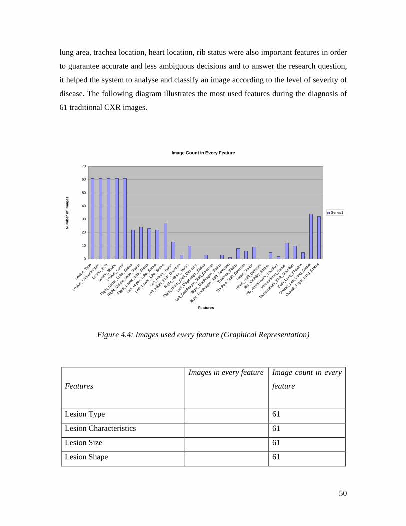
50
lung area, trachea location, heart location, rib status were also important features in order
to guarantee accurate and less ambiguous decisions and to answer the research question,
it helped the system to analyse and classify an image according to the level of severity of
disease. The following diagram illustrates the most used features during the diagnosis of
61 traditional CXR images.
Image Count in Every Feature
0
10
20
30
40
50
60
70
Lesio
n_Typ
e
Lesio
n_Cha
racter
stics
Lesio
n_Size
Lesio
n_Shap
e
Lesio
n_Cou
nt
Right_Upp
er_Lob
e_Stat
us
Right_Middle
_Lobe
_Stat
us
Right_Lo
wer_lob
e_Stat
us
Left_
uppe
r_Lobe
_Stat
us
Left_
Lower_
lobe_
Status
Left_
Hilum_S
tatus
Left_
Hilum_S
hift_D
irecti
on
Right_Hilu
m_Status
Right_Hilu
m_Shif
t_Dire
ction
Left_
Diaphragm
_Stat
us
Left_
Diaphragm
_Shif
t_Dire
ction
Right_Diap
hragm_Stat
us
Right_Diap
hragm_Shif
t_Dire
ction
Trachea_
Status
Trachea_
Shift_D
irecti
on
Heart_S
tatus
Heart_S
hift_D
irecti
on
Rib_Visi
bility
_Status
Rib_Abno
rmality
_Loca
tion
Medias
tinum
_Status
Medias
tinum
_Shif
t_Dire
ction
Both_L
ung_S
hado
w
Overal
l_Left
_Lun
g_Stat
us
Overal
l_Righ
t_Lung
_Stat
us
Features
Num
ber o
f Im
ages
Series1
Figure 4.4: Images used every feature (Graphical Representation)
Features
Images in every feature
Image count in every
feature
Lesion Type 61
Lesion Characteristics 61
Lesion Size 61
Lesion Shape 61

51
Lesion Count 61
Right Upper Lobe Status 7,8,11,27,28,31,32,38,4
0,45,47,55,
58,62,63,50,40,39,62,6
9,70,75
22
Right Middle Lobe Status 15,17,19,28,32,35,38,3
9,41,44,45,46,47,51,55,
58,62,64,68,65,71,
74,75,72
24
Right Lower lobe Status 5,6,10,15,19,27,28,31,3
5,39,42,47,51,53,54,55,
58,62,65,72,74,73,75
23
Left upper Lobe Status 3,4,9,10,13,27,28,29,41
,43,44,47,48,49,51,55,5
7,59,61,66,68,75,
22
Left Lower lobe Status 51,30,29,75,26,1,60,59,
34,54,28,48,47,13,7,4,3
,2,,55,44,66,70,63,68,6
1,73,71,
27
Left Hilum Status 3,26,46,51,55,59,64,66,
67,68,71,73,75
13
Left Hilum Shift Direction 46,51,59 3
Right Hilum Status 10,28,35,46,64,66,68,7
1,74,75
10
Right Hilum Shift Direction 0
Left Diaphragm Status 35,66,67 3
Left Diaphragm Shift Direction 0
Right Diaphragm Status 35,41,63 3
Right Diaphragm Shift Direction 41, 1
Trachea Status 32,40,44,48,61,63,69,7 8

52
5
Trachea Shift Direction 40,44,48,61,63,69 6
Heart Status 40,51,54,60,6,72,73,51,
74
9
Heart Shift Direction 0
Rib Visibility Status 3,44,47,48,62 5
Rib Abnormality Location 44,47 2
Mediastinum Status 10,28,39,48,44,51,54,5
7,61,63,66,67
12
Mediastinum Shift Direction 39,44,48,51,54,57,61,6
3,66,67
10
Both Lung Shadow 67,9,66,44,58 5
Overall Left Lung Status 1,2,3,4,9,13,26,27,28,2
9,30,34,35,43,44,47,48,
49,51,52,54,55,57,59,6
0,63,64,66,67,69,70,71,
73,75
34
Overall Right Lung Status 5,6,7,8,9,10,11,17,27,3
1,32,42,40,41,44,45,46,
47,38,50,51,52,53,54,5
5,58,62,65,68,69,70,74,
32
Table 4.4: Images used in every feature (Tabular Representation)
Total Number of Images 80
Total Number of Images Used for Feature 61
Total Number of Distinct Lung Diseases 65
Total Number of Healthy Lung Image 1
Total Number of Images Not used for Feature 19
Table 4.5: Number of Images used for feature and image interpretation

53
On the other hand, a qualitative measure was taken to choose the five most important
features. First, the most used features were ranked and then the features, that could be
extracted using the proposed algorithm, were chosen. Other important features were taken
into consideration while analysing the image using the image processing techniques. This
means that several other important features were analysed by the system but were not
taken into consideration in the classification according to the severity level of diseases.
This process therefore has provided the opportunity to expand the research further and to
work with other important features. Moreover, other important features had already been
studied in other research. As a result, this trade off assisted in answering the research
question thoroughly. This research has concentrated on classifying 80 images according
to the severity of diseases rather than accurately identifying abnormalities and disease
names.
4.9. Feature Selection
After in-depth study of the important features, the following five features were chosen as
those that were most likely to be able to answer the research question reliably:
Left Lung area
Right Lung area
Trachea area
Rib and Hilum area
Nodule area
4.10. Development of Rules
Just as it was important to understand the interpretation process of the traditional CXR
images, it was also important to understand the interpretation of the patient symptoms
that indicate different lung diseases. Patient symptoms of course also play a vital role in
the decision regarding what disease a patient might have. The traditional CXR image

54
might have similar opacities or shadows that indicate different diseases and the symptoms
help the practitioners to advice, prognoses and decide the disease.
The combination of X-ray image diagnosis and patient symptom diagnosis helps
practitioners to decide what category and what level of a disease a patient is. Although, in
this study patient disease symptoms had not been used for the classification of images
according to the severity of diseases, the diseases that cause different symptoms were
studied. An understanding of different symptoms was equally needed for a better
knowledge domain to back up CXIP with valuable information. A single sysmptom or a
set of symptoms are divided into non significant alphabetical order so the CXIP can apply
a rule or a combination of rules (see Section 5.6.17) based on symptoms for the
determination of lung diseases.Figure 4.5 demonstrates several of the most important
symptoms in the determination of lung diseases. The symptoms were divided into 10 rule
groups. The rule groups for symptoms described in Figure 4.5 are indicated in Table 4.6
for a better understanding.

55
Figure 4.5: Instance of the symptoms diagnosis process
If age > 40 and history of having lung disease in the family tree then
If age> 40 and worked in a place with environmental pollution then
If smoke = yes, number of cigarettes per day >=40 and smoking habit >20 years then
If (age>40 and age<60)
If smoking then
if age >40 then
If family members had/have lung diseases then
If exposure to uranium, radon or asbestos, nickel, arsenic, carcinogens, chloride,
chromium, vinyl then
If frequently coughing then
If coughing up blood then
If wheezing then
If hoarseness found then
If shortness in breath then
If coughing up sputum
If fever with coughing up dark sputum then}
If persistentchest pain then
If drooping eyelid then
If pain in arm or armpit then
If pupil of eye becomes smaller and one side of face sweats less than the other then}
If pain in bones in spine, bones in thigh then
If persistent Headache then
If nausea then
If vomiting then
If loss of bowel or bladder control then
If weakness then
If significant weight loss then

56
Symptom Rule Description Rule Group
If smoking then A
if age >40 then B
If family members had/have lung diseases then C
If exposure to uranium, radon or asbestos, nickel, arsenic, carcinogens,
chloride, chromium, vinyl then
D
If frequently coughing then E
If coughing up blood then E
If wheezing then F
If hoarseness found then F
If shortness in breath then F
If coughing up sputum F
If fever with coughing up dark sputum then} F
If persistent chest pain then G
If drooping eyelid then H
If pain in arm or armpit then H
If pupil of eye becomes smaller and one side of face sweats less than the
other then}
H
If pain in bones in spine, bones in thigh then I
If persistent headache then I
If nausea then I

57
If vomiting then I
If loss of bowel or bladder control then} I
If weakness then J
If significant weight loss then J
Table 4.6: Rule Group classification for lung disease symptoms
On the other hand, for every diagnosis of each traditional CXR image, one informal rule
was created for every image and the accompanying diagnosis details. Examples of rules
for several images are shown in Table 4.7 (See Appendix D for the rules of other
images).
Image
No
Rule Description
1 if large central lesion or white circular mass found then non small cell lung
cancer
2 if volume loss or white mass and pleural effusion at the left lower lobe of lung
then lung cancer
3 if irregular white mass or collapse in left lung then lung cancer (endobronchial
carcinoma)
4 if irregular white mass or collapse in the whole left lung then lung cancer
(endobronchial carcinoma)
5 if a clear cavity or ring cavity with white mass boundary and lucency inside in
the right lower lobe then lung cancer (squamous cell carcionoma)
6 if opacity or shadow (any specific density(whiteness) or lucency(blackness)) and
not well circumscribed in the right lower lobe then lung cancer (squamous cell
carcinoma)
7 if lesion or whiteness in the right upper lobe then lung cancer adenocarcinoma.∗

58
8 if irregular white mass or collapse and the actual size and shape are not
consistent in the right upper lobe then lung cancer (carcinoma)
9 if large mass with opacity or shadow (any specific density(whiteness) or lucency
(blackness)) in left mid lung throughout the upper lung then small cell cancer/ if
nodule or ring with clear whiteness or cavity with white boundary and lucency
in the middle then lung cancer ª
10 if opacity or shadow (any specific density (whiteness) or lucency (blackness)) in
right hila or volume loss then small cell lung cancer/if volume loss or whiteness
with destruction of the proper shape and size of the right lower lobe then small
cell cancer/if whiteness or shadow in the hilar or the mediastinal mass then small
cell lung cancer. ª
* = weak rule ª = multiple rule
Table 4.7: Sample rule descriptions taken from CXKB
The overall rule for the whole diagnosis process can be written in the following algorithm
shown in Figure 4.6. These rules were simplified further before being implemented in the
CXIP.

59
Figure 4.6: Instance of the lung abnormality diagnosis process
4.11. Simplification of Rules
The rules found from every image (Table 4.7 or See Appendix D) and the generic rules
mentioned in Figure 4.6 were further modified and simplified. The simplification process
is shown in Table 4.8 and Table 4.9. This phase of simplification was also done using
linguistic expression that is still not in a formal logic for computational processing.
If there is no white mass in the lung area and the shape of lung, heart, trachea,
diaphragm and mediastinum looks normal then
No sickness
ElseIf there is a white mass in the lung area then
If the white mass has light spot(s) with irregular and poorly defined borders
and is not uniform in density then
probably tuberculosis
If a white mass is found on the outer boundaries of the lungs then
it is probably adenocarcinoma
If a white mass can be found in the joints of the bronchi and the lung then
it is probably squamous cell carcinoma
If the white mass has no defined shape and it changes the boundary of the lung
then
it is pleural effusion or collapse or consolidation.
If the white mass has a small, round or nearly circular shape and it is located
in the outer third of the lungs, especially in the subpleural region of the lower
zones then
it is a nodule
End if

60
Rule Feature Value Severity Level
Rule 1 x1: lesion: size large Medium Level
sickness
x2: lesion: shape circular
x3: lesion: characteristics whiteness
Rule 2 x4: lesion: size medium Low Level sickness
x5: lesion: shape circular
x6: lesion: characteristics blackness/darkness
Rule 3 x7: lesion: size big High Level sickness
x8: lesion: shape oval/ring cavity
x9: lesion: characteristics whiteness & blackness
Rule 4 x10: lesion: size big High Level sickness
x11: lesion: shape irregular
x12: lesion: shape White/black region >1
Rule 5 x13: lesion: characteristics whiteness Low Level sickness
Rule 6 x14: lesion: characteristics blackness Low Level sickness
Rule 7 x15: lung proportion very low High Level sickness
Rule 8 x16: lung proportion normal Normal
Rule 9 x17: lung proportion very high High Level sickness
Table 4.8: Rule Description in Linguistic terms

61
Decision
Matrix
Lesion
Size
(m1)
Lesion
shape
(m2)
Lesion
characteristics
(m3)
lung
proportion
(m4)
Output
R1 large circular whiteness normal Medium Level
sickness
R2 medium circular blackness normal Low Level
sickness
R3 big oval whiteness +
blackness
normal High Level
sickness
R4 big irregular white spot > 1 very low High Level
sickness
R5 whiteness Medium Level
sickness
R6 blackness Medium Level
sickness
R7 very low High Level
sickness
R8 normal Normal
R9 very high High Level
sickness
Table 4.9: Decision matrix in linguistic expression
4.12. Determining the Severity Level
For the classification of images according to the severity of diseases, seven different
types of classification levels were created. The severity levels were determined between
zero to six. The reason for doing this has also been discussed in the previous sections.
The concept of classifying the images according to the severity of diseases is actually an
improvement on and extension of the strategies proposed by Watman et al. (Watman &
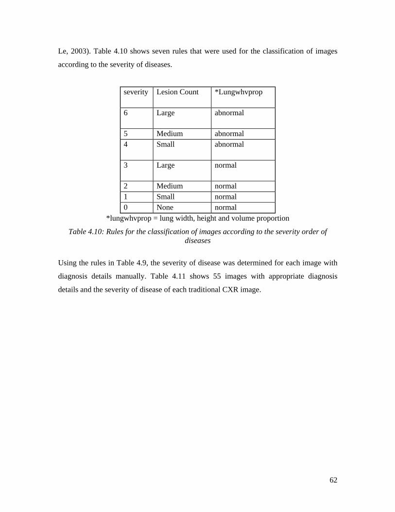
62
Le, 2003). Table 4.10 shows seven rules that were used for the classification of images
according to the severity of diseases.
severity Lesion Count *Lungwhvprop
6 Large abnormal
5 Medium abnormal 4 Small abnormal
3 Large normal
2 Medium normal 1 Small normal 0 None normal
*lungwhvprop = lung width, height and volume proportion
Table 4.10: Rules for the classification of images according to the severity order of diseases
Using the rules in Table 4.9, the severity of disease was determined for each image with
diagnosis details manually. Table 4.11 shows 55 images with appropriate diagnosis
details and the severity of disease of each traditional CXR image.

63
Image No
Lesion Count
Right Lung Status
Left Lung Status
Hilum Status
Diaphragm Status
Trachea Status
Heart Status
Rib Visibility Status
Severity Level/6
1 single ok abnormal abnormal ok Ok ok ok 42 Single ok abnormal ok ok Ok ok ok 43 Single ok abnormal abnormal ok Ok ok abnormal 44 single ok abnormal ok ok Ok ok ok 65 single abnormal ok ok ok Ok ok ok 16 single abnormal ok ok ok Ok ok ok 48 single abnormal ok ok ok Ok ok ok 59 multiple abnormal abnormal ok ok Ok ok ok 5
10 single abnormal abnormal ok ok Ok ok ok 511 single abnormal ok ok ok Ok ok ok 512 multiple ok ok ok ok Ok ok ok 613 multiple ok abnormal ok ok Ok ok ok 214 none ok ok ok ok Ok ok ok 015 multiple abnormal ok ok ok Ok ok ok 119 single abnormal ok ok ok Ok ok ok 621 Single abnormal ok abnormal abnormal Abnormal abnormal abnormal 626 single ok abnormal abnormal ok Ok ok ok 427 multiple abnormal abnormal ok ok Ok ok ok 328 multiple abnormal abnormal abnormal ok Ok ok ok 129 multiple ok abnormal ok ok Ok ok ok 430 single ok abnormal ok ok Ok abnormal ok 131 multiple abnormal ok ok ok Ok ok ok 432 multiple abnormal ok ok ok Abnormal ok ok 334 multiple ok abnormal ok ok Ok ok ok 135 multiple abnormal ok abnormal abnormal Ok ok ok 238 multiple abnormal ok ok ok Ok ok ok 339 single abnormal ok ok ok Ok ok ok 640 single abnormal ok ok ok Abnormal ok ok 6
Table 4.11: Traditional CXR image Diagnosis and Severity Level

64
Image No
Lesion Count
Right Lung Status
Left Lung Status
Hilum Status
Diaphragm Status
Trachea Status
Heart Status
Rib Visibility Status
Severity Level/6
41 single abnormal ok ok abnormal Ok abnormal ok 342 multiple abnormal ok ok ok Ok ok ok 443 multiple ok abnormal ok ok Ok ok ok 644 multiple ok abnormal ok ok Abnormal abnormal abnormal 645 multiple abnormal ok ok ok Ok ok ok 647 multiple abnormal abnormal ok ok Ok ok abnormal 648 single ok abnormal ok ok Abnormal ok abnormal 649 single ok abnormal ok ok Ok ok ok 150 multiple abnormal ok ok ok Ok ok ok 453 multiple abnormal ok ok ok Ok ok ok 254 multiple abnormal abnormal ok ok Ok abnormal ok 555 multiple abnormal abnormal abnormal ok Ok ok ok 557 multiple ok abnormal ok ok Ok ok ok 558 multiple abnormal ok ok ok Ok ok ok 459 multiple ok abnormal abnormal ok Ok ok ok 560 multiple ok abnormal ok ok Ok ok ok 661 single ok abnormal ok ok Abnormal abnormal ok 562 single abnormal ok ok ok Ok ok abnormal 563 single ok abnormal ok ok Abnormal abnormal ok 564 multiple abnormal ok abnormal ok Ok ok ok 165 single abnormal ok ok ok Ok ok ok 466 single ok abnormal abnormal abnormal Ok abnormal ok 467 single ok ok abnormal abnormal Ok ok ok 468 multiple abnormal abnormal abnormal ok Ok abnormal ok 169 single abnormal ok ok ok Abnormal ok ok 571 multiple abnormal abnormal abnormal ok Ok ok ok 172 single abnormal ok ok ok Ok ok ok 3

65
Image No
Lesion Count
Right Lung Status
Left Lung Status
Hilum Status
Diaphragm Status
Trachea Status
Heart Status
Rib Visibility Status
Severity Level/6
73 multiple abnormal abnormal ok ok Ok abnormal ok 575 multiple abnormal abnormal abnormal ok Abnormal abnormal ok 6
Table 4.11: Traditional CXR image diagnosis and severity level

66
Chapter 5: The MACXI Model, Algorithms and Implementation
Chapter 4 examined the expert CXKB being built to link the activities of radiologists.
This provided insights into the role of today’s state of the art technologies in medical
science and into the complexity and uncertainty surrounding the implementation of KB.
Whereas the preceding chapter focused on the complexities of medical image processing
techniques and the expert knowledge context, this chapter adopts a very different angle,
namely, the need for a system for researchers learning different image processing
techniques and for experts requiring assistance both before and during diagnosis. The
research included an eight-month long software development project. The project was
conducted within the limited laboratory environment and aimed at classifying X-ray
images based on disease severity order. The outcome of the project was an interactive
interface for a digital image processor (CXIP) for classifying X-ray images, which
embodied several image processing design principles mentioned in Chapter 3 for
successful analysis of traditional CXR images.
The following sections summarise, first, the objective of MACXI development. This is
followed by a sketch of the project’s specific goals and development stages; the functions
provided by the final product.
5.1. CXIP’s Manipulation of Images
This involved, first, learning the intricacies of the medical images. Collection
management and selection of images manually has been discussed in depth in Chapter 4.
However, it is necessary to explain how the images were loaded into the system. Every
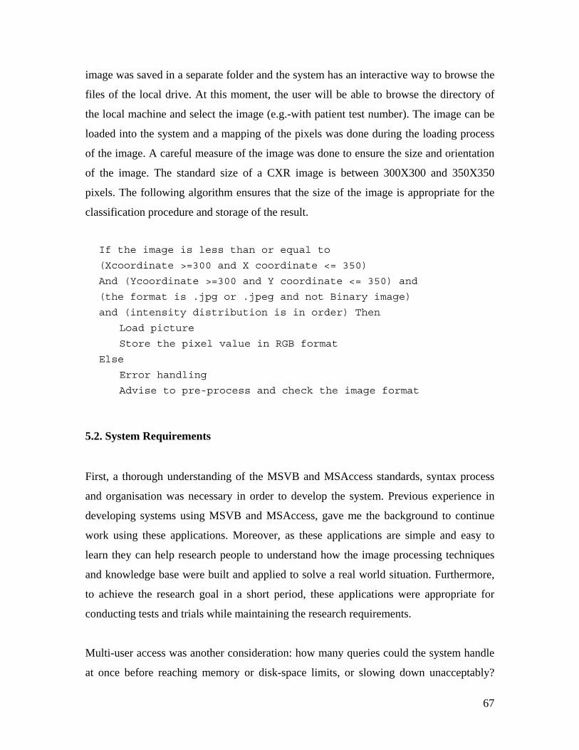
67
image was saved in a separate folder and the system has an interactive way to browse the
files of the local drive. At this moment, the user will be able to browse the directory of
the local machine and select the image (e.g.-with patient test number). The image can be
loaded into the system and a mapping of the pixels was done during the loading process
of the image. A careful measure of the image was done to ensure the size and orientation
of the image. The standard size of a CXR image is between 300X300 and 350X350
pixels. The following algorithm ensures that the size of the image is appropriate for the
classification procedure and storage of the result.
If the image is less than or equal to
(Xcoordinate >=300 and X coordinate <= 350)
And (Ycoordinate >=300 and Y coordinate <= 350) and
(the format is .jpg or .jpeg and not Binary image)
and (intensity distribution is in order) Then
Load picture
Store the pixel value in RGB format
Else
Error handling
Advise to pre-process and check the image format
5.2. System Requirements
First, a thorough understanding of the MSVB and MSAccess standards, syntax process
and organisation was necessary in order to develop the system. Previous experience in
developing systems using MSVB and MSAccess, gave me the background to continue
work using these applications. Moreover, as these applications are simple and easy to
learn they can help research people to understand how the image processing techniques
and knowledge base were built and applied to solve a real world situation. Furthermore,
to achieve the research goal in a short period, these applications were appropriate for
conducting tests and trials while maintaining the research requirements.
Multi-user access was another consideration: how many queries could the system handle
at once before reaching memory or disk-space limits, or slowing down unacceptably?

68
Managing CXIP brought another set of questions. Any pre-processing of the images
reduced the need to process them on the fly; but how many files, or how complex a data
structure, were we willing to maintain? Considerable trial-and-error was needed to
resolve these questions.
A number of other issues were also addressed such as hardware and operating systems
(OS); it was assumed that Microsoft OS are more user friendly and more accessible than
any other available OS. As a result, building a system in this environment allows more
people to access and understand the system. On the other hand, a better trade off cannot
be established to allow users use the system in an old hardware configuration. Although
the system will definitely work, the process will be time consuming. As a result, the
minimum requirements are set to an Intel Pentium III machine or equivalent with a RAM
of at least 64 MB.
5.3. CXIP Implementation and Functionality
MACXI is useful for a wide variety of purposes, given that it combines the expert
understanding, patient history and image processing techniques for a vision that involves
the classification of images. Making MACXI a part of an online medical advisory system
such as Medical Advisory System (MEDADVIS) (Al-kabir, Le & Sharma, 2005) was
taken into consideration.
The current CXIP prototype also served as a pilot study for an ultimate computer aided
tool for any windows-based medical environment. Through the Systems Development
Research Method (SDRM), an understanding of traditional X-ray image diagnosis
interpretation by radiologists and experts was built with an in-depth view of the technical
components involved, their interconnection, and interdependence. MACXI was
implemented in a laboratory environment. However, mathematical and statistical
understanding was also addressed at the suggestion of members of the academic staff at
the University of Canberra. The following sections describe CXIP functionality and
implementation details.

69
5.3.1. CXIP Interface
The first task was to change the interface components by adding several more
functionalities that allowed the user to browse a local directory. As a result, the design for
directory browse was created in such a way as to allow the user to browse the local
directory only for .jpg and .jpeg images. This includes the possibility of users making
mistakes by choosing images in different format. On the other hand, the design applied
that will show only X-ray images as opposed to other types of images in .jpg format. So,
images that are not X-ray images will not be shown. The following naming convention
for X-ray images has been used:
Every image contains x as a prefix with the patient number and the test number
constituting the remainder of the name. The convention thus appears as follows:
If the patient number is 0032 and the test number is 01 then the format will be as
X0032_01.jpg.
The system will also allow the user to search for and locate an image by the test number
for a specific patient. However, it has not been implemented in current version yet. The
interface viewed by the user of this system is illustrated below. The Interface allows the
user to do all the processing in one interface. Figure 5.1 shows the prototype of the
Interface at the initial stage.

70
Figure 5.1: Traditional CXR CXIP interface (before loading image)
First, the user needs to load an image. The user can browse different directories and
folders to choose the image he/she wants to process for classification. Whenever the user
selects the image and double clicks on the image name, the system loads the image by
storing the pixel values in an array.
5.3.2. Image Selection Menu
The following part of the interface deals with the image selection options. The user is
able to browse the local directory and choose the desired image.

71
Figure 5.2: Image selection menu
When the user chooses the desired image and double clicks on it, the following algorithm
is performed to load the image:
Show the image details in a text box
Maximum size of x axis <- maxwidth - 1
Maximum size of y axis <- maxheight - 1
Set array
For x = 0 to maximum size of x axis
For y = 0 to maximum size of y axis
Get colour for point(x,y)
Set graylevel[] <- color
Set slope(x,y) = slope(x,y,slopesquare)
Set slopeX(x,y) = slopeX(x,y,slopesquare)
Set slopeY(x,y) = slopeY(x,y,slopesquare)
Next y
Next x
During the loading process, the system puts the gray value for each pixel point in an
array. Moreover, the slope of X direction, Y direction and in both directions is calculated
and stored. The slopes of the X coordinates, the Y coordinates and for the XY
coordinates are calculated as below:
SlopeX(x,y) = (grayvalue (x + 1, y) - grayvalue(x - 1, y))/2

72
SlopeY(x,y) = (grayvalue (x, y + 1)- grayvalue(x, y - 1))/2
SlopeXY = Sqr root (slopeX(x,y) * slopeX(x,y) + slopeY(x,y) *
slopeY(x,y))
After trying a number of parameters, SlopeX and SlopeY at each point were divided by 2
giving a better approximation for the gradient and edge determination for traditional X-
ray images. This gradient value was used for the normal thresholding operations to isolate
and extract the scapula and lung region. However, it did not give a better result in the
classification of the lung area whenever the images with different intensities increased.
As a result, a morphological gradient determining technique was used at the later stage of
the development. This gave better result than using the normal gradient image. The
interface (Figure 5.3) loads three copies of the same image on three separate frames of
the interface.
Figure 5.3: CXIP interface
The user can select any of the frame boxes and see different results. The system provides
a very powerful tool that enables the user to select the image area to process. It gives the

73
user and the system to negotiate the area that the user wants the system to process. On the
other hand, user selection allows the system to respond with an accurate answer and with
less computational time. The tool is called a “mouse driven frame box”. This tool will
allow the user to select a rectangular or square area to be processed by the processor.
Using the tool is very simple. The user needs to select a starting point and drag the mouse
to an end point in a diagonal direction. Whenever the system gets the start and the end
points, it forms a rectangle where the start point is the lowest x, y coordinates and end
point is the highest x, y coordinates of the mouse driven frame box. Moreover, the
processor determines the centre of the requested rectangle/square by placing a small,
pointed ball at the centre of the frame box. If the user does not select the region, the
system will determine the most suitable region to be processed automatically.
Figure 5.4 shows the mouse driven frame box :
Figure 5.4: Mouse driven frame box.
The following two frames show different features of histogram findings:

74
Figure 5.5: Histogram analysis board
Figure 5.6: Pixel values are shown inside the histogram analysis board
In the following sections, the different image processing techniques that are used to
classify images according to the severity of diseases are demonstrated and described.
During development, numbers of assumptions and tests were undertaken. As a result,
different versions demonstrate the different approaches that were adopted to extract
features successfully. As every image contains a maximum of 122500 pixels, it is not
considered realistic to process all the pixels together. As a result, a different structuring
element or window or mask (Baxes, 1994; Schalkoff, 1989; Jain,1989; Wilson, 1992)
was used to process every pixel by comparing a number of neighbour pixels. In this
research, several operations using a 3X3, 5X5 window size or mask size were performed
by keeping the target pixel at the centre. Several operations were also performed using
7X7, 9X9, 11X11, 25X25 windows depending on the results. Determining a good
window or mask size depends on the image. It was a trial and error based technique and
the window size was chosen based on the best result. However, the computational costs
were another major factor. For example, when the image was processed using an 11X11

75
window, the processing was extremely slow. As a result, a trade off was made by
reducing the window size and using other parameters. The large-sized window was only
used when the image area was small.
In other words:
The size of a window was inversely proportional to the size of the image area to be
processed.
For segmentation and for the identification of edges and boundaries, a combination of
thresholding, morphological and region growing techniques was used to extract the
features and to classify images according to the severity of diseases.
The rest of the chapter demonstrates the artefact functionality as well as the techniques
used to achieve the successful classification of images by the system according to the
severity rules developed during the CXKB development phase of the research.
The neighbourhood connectivity depended on the mask at different stages of the
processing. All the masks used all connected neighbourhood technique during the
processing,. For example, if the window size is 3X3 then the neighbourhood connectivity
is eight connected. If the window size is 5X5 then the neighbourhood connectivity is 24
connected. Accordingly, the neighbourhood connectivity can be written as below:
If the window size is nXn then the neighbourhood connectivity is n.n-1 where n is
1to 25.
5.3.3. Perform Dilation
Whenever the user selects dilation (Gil & Kimmel, 2000; Droogenbroeck, 2005), CXIP
performs the following algorithm using a 3X3 or a 5X5 structuring element. If I(x,y) is

76
the pixel to be processed and if Xn are the neighbouring pixels then the output value of
the dilation is
O(x,y) = max(Xn, I(x,y)) where n = 1 to 8
Figure 5.7: Dilated images: dI (x,y)
5.3.4. Perform Erosion
Whenever the user selects erosion (Gil et al., 2000), CXIP performs the following
algorithm using a 3X3 or a 5X5 structuring element.
If I(x,y) is the pixel to be processed and if Xn represents the neighbouring pixels then the
output value of the erosion is O(x,y) = min(Xn,I(x,y) where n = 1 to 8
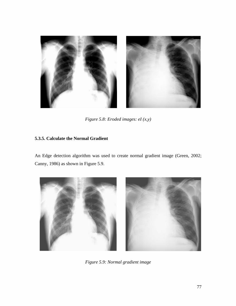
77
Figure 5.8: Eroded images: eI (x,y)
5.3.5. Calculate the Normal Gradient
An Edge detection algorithm was used to create normal gradient image (Green, 2002;
Canny, 1986) as shown in Figure 5.9.
Figure 5.9: Normal gradient image

78
5.3.6. Calculate the Morphological Gradient
Having established the dilation and erosion for every pixel, the next task was to
determine the morphological gradient (Baxes, 1994; Dougherty & Loce, 1992; Rivest et
al., 1993) which is the subtraction between the dilated image and the eroded image using
a dual image point process. The algorithm can be written as follows: O(x,y) = dI(x,y) – eI(x,y)
Figure 5.10 shows two morphological gradient images after performing the above
algorithm.
Figure 5.10: Morphological gradient images
5.3.7. Calculate the Morphological Reconstruction
When using morphological image processing, morphological image reconstruction
(Beucher et al. 1990; Beucher, 1991; Qian & Zhao, 1997)) is a very valuable technique
that reduces the number of local maxima and minima by averaging connected
components. This technique creates large plateaus, catchment basins and peaks by giving
one selected gray level value to a similar set of gray level values. This process is actually

79
a combination of dilation and erosion. First of all, two marker images are created from
the initial eroded and dilated images. The algorithm is: O(x,y) = eI(x,y)-1
O(x,y) = dI(x,y)+1
After this, a 3X3 or 5X5 window was used to give the centre pixel the highest value and
create another image set. This process was performed three times. Omax(x,y) = max(Xn, I(x,y)) --- perform 3 times
In addition, another image set was also created by giving the target pixel the lowest gray
value. This process was also performed three times. Omin(x,y) = min(Xn,I(x,y)) --- perform 3 times
The third image set for the above two algorithms was used to determine the point wise
maximum and point wise minimum for each pixel and to create another two sets of
images. The algorithm is described below:
To get the point wise minimum If Originial(x,y) >= Omax(x,y) then
Opointmin(x,y) = Original(x,y)
Elseif Original(x,y) <= Omax(x,y) then
Opointmin = Omax(x,y)
To get the point wise maximum If Originial(x,y) < Omin(x,y) then
Opointmax(x,y) = Original(x,y)
Elseif Original(x,y) <= Omin(x,y) then
Opointmax = Omin(x,y)
The following algorithm reconstructs the minima and maxima images: Oreconminima(x,y) = Original(x,y) – Opointmin(x,y)
Oreconmaxima(x,y) = Opointmax(x,y) – Original(x,y)
Next, a combination of opening and closing by reconstruction are performed: O(x,y) = I{closing}(x,y)
O(x,y) = I{opening}(x,y)
Dilation was again performed on the Omax(x,y) image as below: Omax = max (Xn,Imax(x,y)
Erode the previously produced image five times and the algorithm is: Omin = min (Xn,Imin(x,y) --- perform 5 times

80
Figure 5.11 shows morphologically reconstructed images.
Figure 5.11: Morphologically reconstructed images (multiple reconstructions)
5.3.8. Determine the Regional Minima and Maxima
The next step was to determine the regional minima and maxima (Moga & Gabbouj,
1997; Beucher, 1983). In this research, the minima to extract the features were utilised.
The previous image was dilated out and then the new copy of the image was eroded again
three times again. The combination of dilation and erosion was used to remove the
occluded parts and blobs from the image. Odil(x,y) = max(Xn,Omin(x,y))
Oero(x,y) = min(xn, I(x,y)) --- perform 3 times
The regional maxima and minima were calculated using the following algorithm: For i = 1 to windowsize
If targetpixel = Xn(i)
count = count +1
End if
Loop

81
If count >=windowsize-1 and I(x,y){this image is the image that
had been created at the five consecutive erosion at the
previous stage} >= meangrayvalue then
Targetpixel{regionmaxvalue}(x,y) = 255
Elseif I(x-1,y) <= lowestgrayvalue
Targetpixel {regionmaxvalue} (x, y) = 0
Else
Targetpixel {regionmaxvalue} (x, y) = -1
End if
5.3.9. Label Minima and Maxima
A labelling technique was used to label the minima and maxima (Moga & Gabbouj,
1998) for every region. The algorithm is described below:
For i = 0 to picxmax
For j = 0 to picymax
Set 7X7 window on I(x, y)
If I{regionmaxvalue}(x,y) = 0 and I{labelstampmin}(x,y) = 0
then
For m = x-3 to x+3
For n = y-3 to y+1
If I{labelstampmin}(m,n) > 0 and I{regmaxval}(m,n) =0 then
I{labelstampmin}(x,y) = I{labelstampmin}(m,n)
For s = x-3 to x+3
For t = y -3 to y+3
I {labelstampmin}(s,t) = I{labelstampmin}(x,y)
Next t
Next s
Exit
Elseif I {labelstampmin}(m,n) = 0 and
I{regionmaxval}(x,y) = 0
counter = counter + 1
End if
Next n
Next m

82
If counter >= 49 Then
For m = x - 3 To x + 3
For n = y - 3 To y + 3
I{labelstampmin}(m, n) = LabelMinLcounter
Next n
Next m
LabelMinLcounter = LabelMinLcounter + 1
End If
End if
Next j
Next i
Figure 5.12 shows the target regional minimum of two images labelled in red colour.
Figure 5.12: Images of regional minima labelled (in red)
5.3.10. Distance Calculation
Figure 5.13 shows the distance transformed image (Meijster, Roerdink, & Hesselink,
(2000); Preteux, 1992) of the morphologically reconstructed image (Figure 5.11). The
morphologically reconstructed image, minima labelled image and distance image were
used to trace the boundary of the scapula, the trachea, the diaphragm and the lung areas.

83
Figure 5.13: Distance images
5.3.11. Histogram Analysis
Using the actual gray level value and the reconstructed gray level value, histograms
(Astola, Koskinen & Neuvo, 1992) for actual image and reconstructed image were
created. Figure 5.14 shows the histogram diagram of the actual image and Figure 5.15
shows the histogram diagram of the reconstructed image. The x direction indicates the
gray level and the y direction indicates the number of pixels that have a particular gray
value or reconstructed value. The histograms were used to perform the propagation
process in the morphologically reconstructed image (Figure 5.11).

84
Figure 5.14: Histogram of an actual image
Figure 5.15: Histogram of a morphologically reconstructed(multiple) image

85
5.3.12. Propagate Regions
The Propagation (Lotufo & Falcao, 2000; Meyer, 2000; Rambabu Rathore &
Chakrabarti, 2003) algorithm (See Appendix H-Pseudocode for Propagation) was used to
grow each region from the selected minima determined in the previous algorithm. The
minima were selected. The minima expands its region based on the gray value being
equal to or higher than the minima value that ultimately stops near the region outside the
lung area. This was the key process of the entire processing. The first task was to
determine which minima region needed to be selected to perform the propagation
process. The best starting point from all the minima regions was actually the
rectangular/square outer boundary of the image. As a result, the propagation algorithm
started from the outer boundary of the image. This is strongly recommended to ensure the
quality of the images as is discussed in Chapter 4. Each pixel is given a label value. A
component labelled image (Cypher, Sanz & Snyder, 1990; Cypher, Sanz & Snyder, 1989;
Alnuweiri & Kumar, 1991) is created where every pixel receives a gray value of zero (0)
or one (1). Figure 5.16 shows images after the propagation algorithm is performed on
morphologically reconstructed and distance images.
Figure 5.16: Image after propagation

86
5.3.13. Lung Region Extraction
A binary image was then created giving the labelled pixels 0 and the unlabelled pixels 1.
This process nicely extracted the left and right lung as white and the rest of the area as
black. However, some areas near the trachea, clavicle and diaphragm will have white
holes and blobs and noise between the lung area and near the outer side of both the left
lung and the right lung. To remove noises, holes and blobs, smoothing operation was
performed. The algorithm is described below: For I = picFrame.x1 to picFrame.x 2
For j = picFrame.y1 to picFrame.y2
If I{labelstamp}(i, j) = 1 Then
I{binaryvalue}(i, j) = 0
Else
I{binaryvalue}(i, j) = 1
End If
Next j
Next i
Figure 5.17: Lung region extracted image (with noise, blobs and holes)

87
5.3.14. Smoothing the Image
The smoothing (Nguyen, Worring & Boomgaard, 2003; Leymarie et al., 1989; Derraz,
Beladgham & Khelif, 2004) operation (See Appendix H-Pseudocode for Smoothing
Operation) was used to remove the remaining small blobs, noise and holes from the
binary image. This operation removed the blobs near the upper trachea area in between
and slightly above the lung area. The smoothing operation determined the trachea area
and removed the white hole of the upper part of the trachea.
Moreover, the smoothing algorithm calculated the distance between two lungs from the
upper inner left and right lobe of the image. The algorithm looked at the white (1 valued)
connected components that are not lung area by detecting the size and geometry of the
white (1 valued) connected regions. If the size of a white connected region has a circular,
rectangular or square shape with a size of less than 1400 pixels, the smoothing algorithm
assigned zero (black) to those pixels.
Moreover, it also looked at the size of the trachea. The trachea region usually has a
rectangular shape where it has a different height and width and the height is higher than
the width. The height was calculated vertically and the width was calculated horizontally,
and if it is found that the height and width of that area is different and the area of the
rectangle is more than 800 pixels and less than 1400 pixels, then it was taken as the upper
part of the trachea. At this point, my system can detect the upper part of the trachea and
clavicle. These areas were assigned a zero (black) value during the smoothing process for
a better classification process.

88
Figure 5.18: Lung region extracted image after smoothing
5.3.15. Isolation of the Left and Right Lung Areas
When the smoothing algorithm is performed, it assigns a zero value to all the regions
except the left and right lung area that can be visualised by a radiologist. However, when
a lung area is not visible or when a collapse or consolidation is present, what does a
human expert do? What does an expert do to recognise the pattern for a lung area and
differentiate the perceived lung knowledge from the lung area present in a traditional X-
ray image? How can this level of knowledge be put into MACXI? This is the most
complicated process as none of the lung anatomy has a fixed size or pattern. The reason
is that if it is tissue or flesh, the shape changes depending on the patient situation during
the radiographic image capturing process. What happens when the patient takes a deep
breath? The lung actually expands in size. However, the rib area from the middle of the
left and right lung disappears, because air in expanded lung absorbs very little x-radiation
and the anterior part of the ribs move upwards with inspiration. The opposite effect
occurs when the patient only takes a shallow breath. The lung shrinks in size thus
illuminating the rib area. The result is that the X-ray captures the rib area very well but
the left and right lung boundaries become less evident. Therefore, representing these

89
differences using a rule-based system is not possible although some level of success can
be achieved whenever the system finds dissimilarity in the size and geometry of the left
or right lung.
The usual rule is that the right lung is slightly larger than the left lung. Is that the size? Or
is it the volume? Is it the height? Or is it the width? Moreover, the left side of the heart
area overlaps the lower lobe of the left lung. But, what is the possible size? Again, there
is no proper approximation in finding the proportion of the overlap because this depends
on the level of the X-ray beam transmitted through the patient’s chest. How much should
the patient inhale or exhale? And furthermore, it is difficult to discover an abnormality in
the heart in a case in which it really overlaps the whole lower lobe of the left lung. For
this reason, this last parameter is taken as a least assumption. So, the parameters to reveal
the abnormality in the size of the lung or to detect the collapse or consolidation of the left
or the right lung, the height, width and volume of both lungs in proportion to each other
are used to see if the proportion is higher or less than the threshold. On the other hand, if
the proportion of volume and height (vertical) is less or more than the threshold, the
problem is near the lower lobe of the left or the right lungs. If the proportion of the height
and the width is higher or less than a threshold, it usually means a level of collapse or
consolidation is present in either the left or the right lung. The width and height
proportion is measured or mapped through one rectangle/square for each lung. The
volume proportion is mapped through the pixels inside the left and right lung area.
After the left and right rectangles were determined, the first task was to label the pixel
that belongs to the left or the right lung. When every pixel in either the left or the right
lung was labelled, the total number of pixels for each lung was determined. The
proportion of the total number of pixels for each lung was measured. Whenever, the
proportion is less than or higher than a threshold, a level of abnormality is reported.
Whenever the height and width proportion is above or below a threshold value, a level of
abnormality is also reported.

90
The algorithm for determining the lung width, height and volume can be found in
Appendix H-Pseudocode for Left and Right Lung determination.
Finally, the following algorithm calculates the proportions of lung volume, lung width
and lung height: initialise lungproportion, heightpro, widthpro As 0
lungproportion = (rlungpixelcount / llungpixelcount)
widthpro = ((rxmax - rxmin) / (lxmax - lxmin))
heightpro = ((rymax - rymin) / (lymax - lymin))
Figure 5.19: Left and Right Lung region extracted images
5.3.16. Abnormality Detection
A considerable amount of time was spent building algorithms that included some
constant parameters (threshold) to independently discover patterns (Fukunaga, 1990;
Young & Calvert, 1974; Tveter, 1998; Aylward & Kim, 2004). The algorithm was
performed to detect lung abnormality and any diseases present inside the lung area. This
research tested and evaluated twelve (12) different images by tuning the constant
parameter. The reason for combining lung height, width and volume to establish an

91
average is that this provided improved findings. After an in-depth analysis, it was found
that the sum of the proportions of lung width, height and volume divided by 3 gives a
result between 0.93 and 1.14, which would be regarded as a normal lung finding. On the
other hand, if the average of the sum is below 0.93 and more than 1.14 then there is a
level of abnormality present in the lung size and volume. The constant values are the
knowledge that human experts use during their diagnosis process. The human experts
expect the proportion of the right and the left lung to be 1.1 meaning the right lung is
larger than the left lung. Moreover, the volume of the right lung is also greater than the
volume of the left lung.
If (((lungproportion + widthpro + heightpro) / 3) >= 0.93 and
((lungproportion + widthpro + heightpro) / 3) <= 1.14) or
(lungproportion >= 0.9 and lungproportion <= 1.14) Then
lung_volume_proportion = "Normal"
ElseIf (lungproportion < 0.93) Then
lung_volume_proportion = "abnormal Right Lung"
ElseIf (lungproportion > 1.14) Then
lung_volume_proportion = "Abnormal Left Lung"
End If
If (heightpro >= 0.93 And heightpro < 1.12) Then
lung_height_proportion = "Normal"
ElseIf (heightpro < 0.93) Then
lung_height_proportion = "abnormal Right Lung"
ElseIf (heightpro > 1.12) Then
lung_height_proportion = "abnormal Left Lung"
End If
If (widthpro >= 0.93 And widthpro < 1.12) Then
lung_width_proportion = "Normal"
ElseIf (widthpro < 0.93) Then
lung_width_proportion = "abnormal Right Lung"
ElseIf (widthpro > 1.12) Then
lung_width_proportion = "abnormal Left Lung"
End If
If rlungpixelcount = 0 And llungpixelcount <> 0 Then
lung_proportion = "right lung Collapse"
ElseIf llungpixelcount = 0 And rlungpixelcount <> 0 Then
lung_proportion = "left lung Collapse"

92
End If
5.3.17. Determine Lesion
A 21X21 window was initialised over every pixel of the left and right lung regions. The
task of this window was to determine the gray values that are between two threshold
values. After an in-depth analysis of the images, it was found that the nodules or the
diseased areas of any lung region have a gray value that is usually higher than or equal to
the average of the sum of the mean gray value and the median gray value of each lung
region.
On the other hand, the diseased areas gray value is also less than the difference between
the maximum gray value in that region and the absolute approximate average of the
difference of the maximum gray value and the mean gray value. If the gray value of
pixels under the window is in between the mentioned threshold then a counter is
increased and the window moves to the next pixel. In this way, whenever there are more
than 300 pixels under the 21X21 window that have the value between the threshold
values, the algorithm looks for the shape (e.g. circular, oval or not uniform) of the
diseased area.
To do this, CXIP applied the basic algorithm of the Hough Transform (Parker, 1996;
Nixon 2002). However, it was modified by taking the 21X21 window centre as the centre
of the circle and 21 pixels as the radius of the circle. If all the pixels inside the circle/oval
have the same values between the threshold, then it is an abnormal area.
This process allowed CXIP to exclude detecting the rib area as the diseased area because
whenever the size or shape of the window area is nearly rectangular or square, the

93
window goes another 40 pixels in every direction (NSEW) and checks the rate of change
of gray level. If two of the directions have a higher length than the other direction, this
means that it could be the rib region and thus the system excludes that region.
This is the last processing required to make the classification complete. At this point,
whenever there is less than one nodule detected, it means there is no diseased spot is
found. If there is more than one and less than or equal to two spots present, then there is a
low level lesion present. If there are more than two and less than or equal to six spots
present, then it is a medium level lesion. Finally, if there are more than six
circular/oval/nearly rectangular spots (Geometric Operations-Rotate, 2005) are present,
then the lesion abnormality is high and the lesion shape is not uniform.
Moreover, the size of the lesion is determined by approximately 121, 225, 441, 961 pixels
of rectangular area. The lesion whiteness or blackness is determined by the gray mean,
median, maximum and minimum values divided or multiplied by sever fixed parameters.
Lesion shape has already been discussed in previous paragraph. Currently, the system can
identify approximately 441 pixels of rectangular area very well. Moreover, the lesion
whiteness is calculated accurately by the system.
To a certain extent, other sizes and characteristics are also determined by the system. This
processing only deals with opacity/nodule/spots/ununiformed density well inside the lung
area detected by CXIP. It has an essential meaning with real world diagnosis. When a
human expert looks at an image and finds that the lung shape/volume/height/width has
abnormality, the system does similar processing (See Appendix H- Pseudocode for
Lesion Determination). Figure 5.20 shows the lesion extracted images.

94
Image No: 9 Image No: 11
Figure 5.20: Lesion extracted images
5.3.18. Classification Process
When the lesion size, shape, characteristics, number of lesions, lung area, lung width,
lung height and lung volume are measured by the system, the system fires one of the
seven different rules that were discussed in Chapter 4. These rules label every image with
a level of severity and store the output in the knowledge database. The system
classification according to the severity level of diseases for the 12 images is shown in
Table 5.1.

95
Image No Severity Level (MACXI Output)
1 1
4 6
5 1
6 4
8 5
9 4
10 5
11 5
14 0
21 6
49 1
58 4
Table 5.1: Classification of images (in severity order) by MACXI

96
Chapter 6: Evaluation and Results
This chapter discusses the issues that were explored to answer the research question.
Section 6.1 and Section 6.2 discusses the contribution to the research community and the
importance of the research. Section 6.3 shows the results that were produced by CXKB
equipped with CXIP. The results were evaluated against the severity level determined,
based on diagnosis details for each image.
6.1. Value to the Research Community
The research demonstrated the report of successful use of morpholocial image processing
technique in CAD of lung diseases from CXR images. Morphological image processing
is also claimed to be successful, especially in medical imaging. However, the
implementation of these concepts in a CAD system seemed rather incomplete,
unavailable or vague. No related research was found that used morphological image
analysis as the primary technique for the processing and analysis of traditional X-ray
images. The focus was to process and analyse traditional CXR images for classification
according to the severity of diseases and the research has successfully addressed this
particular case.

97
6.2. Implications
The study found that millions of traditional CXR images are produced every year in the
US. This is the most traditional method for looking at the lung at the initial stage. If
appropriate and reliable statistics were available it could be assumed that at least several
million other images are taken every year all over the world for the diagnosis of lung
diseases. Especially when developing countries and rural areas around the world depend
largely on traditional CXR images for their diagnosis, prognosis and advice, it is
important to isolate the most severe images to act in relation to those patients who have
acute lung diseases. MACXI offers a contribution to the existing CAD technology that
will help other experts or novice operators for the classification of images according to
severity of diseases because this function is performed optimally by the processor.
MACXI has the potential to be life saving equipment, which obviates the need for
patients, would not have to wait months to receive their reports, start medication or
receive further advice or suggestions. This processor will also allow radiologists to
recommend advanced diagnosis that, hopefully, will be quick enough to save lives.
Moreover, this processor is also a learning tool, which enables researchers, and medical
imaging researchers will be able to understand the strengths and weaknesses of using
morphological operations and a combination of morphological techniques and other
techniques before they use these techniques for their research.

98
6.3. Performance
Only 12 different traditional CXR images among the 80 stored traditional X-ray images
stored in CXKB were used to test the processing, analysis and classification process. The
remaining 68 images were not used because the images did not meet the requirements
previously mentioned in Section 4.5 of Chapter 4 (or see Appendix B). Most of the 68
images had some similarities, including incomplete chest anatomical structures,
incomplete diagnosis details, inaccurate orientation, and inappropriate resolution. On the
other hand, the selected 12 images were carefully chosen as being capable of successful
processing by MACXI. The 12 selected images were processed and assessed and then
sent to MACXI for classification. Even this process took a long time because the images
were collected from a variety of sources and most of the images had different
orientations, and intensity levels. There are only a few other similar systems developed
for the X-ray analysis work but were not accessible and hence, the MACXI results could
not be compared with results from other systems.
For each image, the success of the classification process was measured against individual
diagnosis reports made by radiologists and other experts. This was a challenging but
interesting stage of the research. Basically, this improved the classification process and
the results almost matched the decisions made by experts and/or radiologists all the
images. The system classification of images according to the severity of diseases was
successful in 10 of the 12 images. Table 6.1 shows the comparison of the severity levels
based on expert diagnosis details and the system classification output.

99
Image
No
Human Interpreted
(Based on Radiographic diagnosis
details)
Machine Interpreted
(MACXI)
Lesion
Count
Lung Status Severity
Level
Lesion
Count
Lung
Status
Severity Level
1 1 Abnormal 4 1 Normal 1
(Misclassified)
4 2 Abnormal 6 2 Abnormal 6
5 1 Normal 1 1 Normal 1
6 1 Abnormal 4 1 Abnormal 4
8 4 Abnormal 5 4 Abnormal 5
9 4 Abnormal 5 2 Abnormal 4
(Misclassified)
10 4 Abnormal 5 4 Abnormal 5
11 4 Abnormal 5 4 Abnormal 5
14 0 Normal 0 0 Normal 0
21 0 Abnormal
(Collapse)
6 0 Abnormal
(Collapse)
6
49 2 Normal 1 1 Normal 1
58 2 Abnormal 4 1 Abnormal 4
Table 6.1: Comparison of classification in severity order between human expert (based on expert diagnosis details) and MACXI.

100
Image No: 1 Image No: 5
Figure 6.1: Examples of classified images from MACXI
Figure 6.1 (See Appendix F for other images) shows two images classified by MACXI.
According to the diagnosis details of the expert, the level of severity of Image No.1 was
determined as 4 whereas MACXI classified the image with severity level of 1. MACXI
successfully marked the circular region of interest at the upper lobe of left lung; however,
it miscalculated the lung region. The reason for the large discrepancy in the classification
of the image is that MACXI miscalculated the proportions of the lung height, width and
volume ratio (see 5.7.16). On the other hand, the level of severity of Image No.5 was
determined as 1 and MACXI also classified the image with a severity level of 1. In this
case, MACXI successfully calculated the lung region as well as small circular region of
interest at the lower lobe of the right lung.
Approximately 83.33% accuracy was achieved in determining the severity level of
images. The detection of 21 regions of interest in the selected 12 images where it should
have been 25 regions of interest was a major problem faced by CXIP. This means the
system was detecting 1.75 regions of interest per image instead of detecting

101
approximately 2.08 regions of interest per image. As a result, it changed the classification
level decision-making process because the error in the region of interest meant that there
were additional abnormalities (nodule, opacity, density) inside the lung area. The
sensitivity rate (false positive) rate was approximately 4.76 percent or 1 false positive in
the 12 images. On the other hand, the specificity rate was approximately 19.05% or a
total of 4 false negatives in the 12 images.
As the ultimate objective was not to discover the type of abnormality inside the lung, but
rather, to classify the image to a severity level by analysing the whole anatomical
structure of the image, this way of looking at all the abnormalities inside and outside the
lung area was thought to be a worthwhile trade off in order to achieve a better
classification according to the severity of diseases.
However, the classification process becomes deteriorates when the window size for
detecting abnormalities inside the lung region is reduced; a smaller window size results in
more regions of interest by making the classification result inaccurate. On the other hand,
increasing the window size overlooks areas of interest that are true positives or truly
abnormal. This dilemma raised another problem and as a result, the research used trial
and error techniques to determine the best window size for the detection of abnormalities
inside the lung area. The research also applied several morphological operations after
extracting the lung area; however, additional work is needed to ascertain what other
image processing techniques can be amalgamated with morphological operations to more
successfully determine abnormalities inside the lung area.
This research can be further extended by applying fuzzy theory and sets (Watman, C. &
Le, K., 2004) for the detection of fuzzy connected regions (Udupa & Saha, 2004;
Foliguet et al., 2001) and for the classification of images according to the severity of
diseases.

102
Chapter 7: Limitations, Future Directions and Conclusion
7.1. Fulfilment of Project Objectives
The primary objective of the prototype building was to develop a knowledge base
equipped with an image processor for classifying images according to severity of diseases
and to help researchers understand several image-processing techniques in a coded
manner rather than in a conceptual manner. The radiologist/expert version of the
prototype successfully classified 12 different traditional CXR images.
7.2. Conclusion
The proposed model MACXI brings a completely new way of looking at a framework
that can assist the radiologist by classifying images according to the severity of diseases.
MACXI is an entirely new scheme that offers radiologists the opportunity not only to
look at areas of interest (nodules or lung abnormality) but also to focus first on those
images that have a higher level of severity.
This research has demonstrated a traditional CXR analysis and classification model using
the latest science for the classification of traditional CXR images according to the
severity of diseases. Current image processing techniques, tools and methods were also
justified throughout the study.
The MACXI model makes a valuable contribution to the existing knowledge, which
currently lacks a model for the classification of images. Moreover, the proposed model
demonstrated several image-processing techniques that have not previously been used in
analysing traditional X-ray images before. Furthermore, this model included an open

103
source system that can help researchers understand several image-processing systems and
their effectiveness.
On the other hand, this research could not address several issues, which provide new
directions based on this particular research. A fuzzy system or system with ANN, for
example, could be expected to improve the current model’s abnormality selection
process. Moreover, access to an image database as well as medical areas and experts will
allow the model to handle the real environment and the model becoming fully functional
operational in medical areas in the future.
7.3. Research Limitations
The study has a number of research limitations. These are as follows:
Firstly, although it was very important for this research to have strong
communication relationships with experts from different areas of medical science,
the number of experts employed may not be regarded as sufficient for purposes of
statistical analysis. Moreover, experts from different geographical locations were
strongly needed for participation.
Secondly, applying image processing techniques and methods was very important
for this research. However, this requires the contribution of experts from the fields
of engineering, mathematics, information science, statistics and psychology to
identify methods and techniques that will best suit the diagnosis of traditional
CXR images and this was beyond the scope of this individual research.
Thirdly and most importantly, this research had a very tight time constraint, which
restricted the study to one and half year (three semesters). Thus it was not
possible to achieve all the goals and aims of this proposal. Elevation of this
research to PhD level would allow more time and more support to ensure the
complete achievement of the proposed aims and objectives.

104
7.4. Future Directions
The following steps could be taken to extend this research for future directions
• The model might more accurately and successfully identify, analyse and
classify images if FL or ANN were implemented rather than using hard logic.
• The quality of 80 CXR images was manually assessed based on the criteria,
for example- clarity, orientation, completeness, mentioned in Chapter 4. New
functionalities could be added in the current prototype to assess and determine
the quality of images automatically.
• Additional diagnosis details and clinical details as well as the presence of a
radiologist expert could assist in the construction of a better knowledge base
that could deal more efficiently with ambiguity and uncertainty.
• Collection of images with higher resolution and uniform intensity could
improve the model’s classification process considerably.
• Access to patients’ explanations of clinical details and experts’ interpretations
and access to medical institutes could improve the accuracy of the proposed
model significantly.
• Although this system was tested with 12 X-ray images, the system can be
extended to analyse any number of images based on the criteria and
procedures established in Section 4.5.

105
Appendices
Appendix A : Image diagnosis details
Diagnosis details of 80 CXR Images (can be found in Image_Details_For_KB.doc of the
attached CD#1).
Appendix B: Image manipulation and selection
Image Manipulation of 80 CXR images (can be found in
Image_manipulation_&_Selection.doc of the attached CD#1).
Appendix C: Lung disease details
Description of Lung Diseases (can be found in Disease_Details_For_KB.doc of the
attached CD#1).
Appendix D: Individual rule for 80 images
Linguistic Rules for 80 selected images (can be found in
General_Rule_With_Image_Details_For_KB.doc of the attached CD#1).
Appendix E: CXIP and CXKB
See the attached CD#1 for CXIP and CXKB

106
Appendix F: Classified Images
• See 12_Selected_Images folder of the attached CD#1 for 12 pre-processed (before
classification) images.
Image No: 4 Image No: 6
Image No: 8 Image No: 9
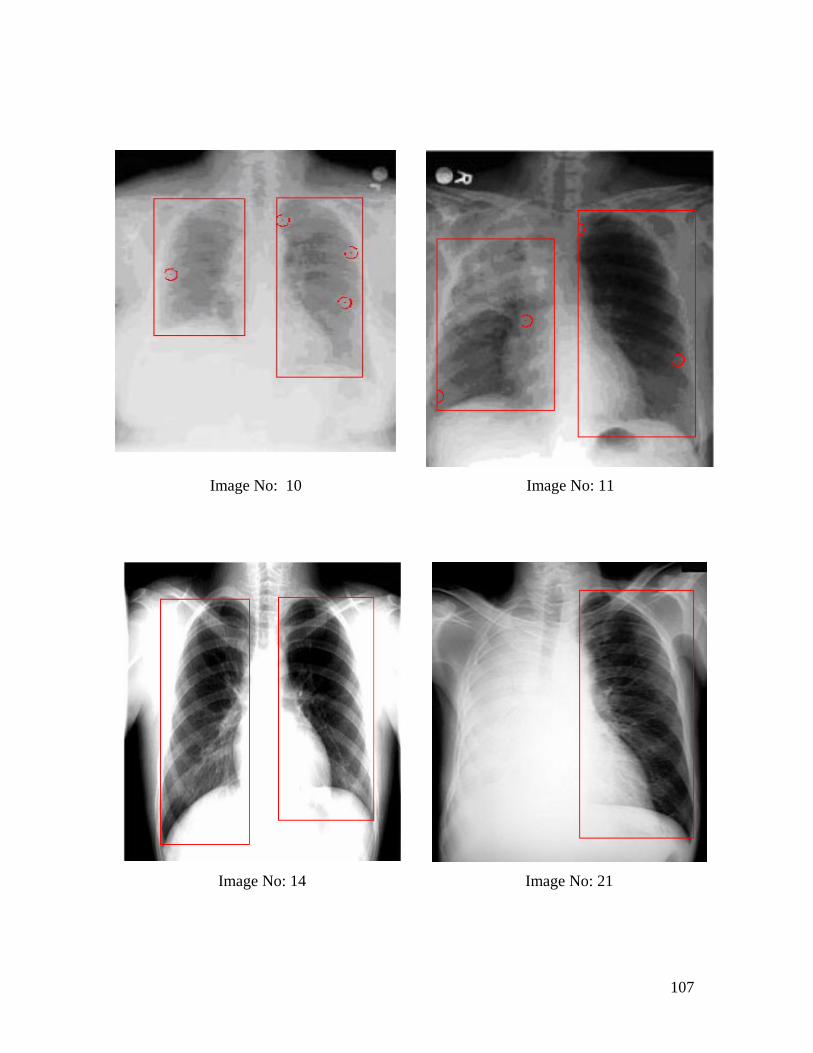
107
Image No: 10 Image No: 11
Image No: 14 Image No: 21
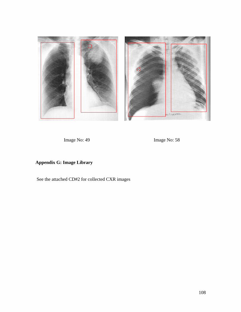
108
Image No: 49 Image No: 58
Appendix G: Image Library
See the attached CD#2 for collected CXR images

109
Appendix H: Pseudocode
Pseudocode for Propagation
initialise array histox(m,n) = -1 and histoy(m,n) = -1 to store
x and y coordinates where m = 0 to 255 and n = 1 to 100000
initialise array histo(r) where r = 0 to 255
For x = picFrame.x1 To picFrame.x2
For y = picFrame.y1 To picFrame.y2
If I{reconstructed}(x, y) < 0 Then
I{ reconstructed}(x, y)= 0
ElseIf I{ reconstructed}(x, y) > 255 Then
I{reconstructed}(x, y)= 255
End If
r = I{reconstructed}(x, y)
histo(r) = histo(r) + 1
Next y
Next x
For n = 0 To 255
m = 0
For x = picFrame.x1 To picFrame.x2
For y = picFrame.y1 To picFrame.y2
If n = I{reconstructed}(x, y)Then
histox(n, m) = x
histoy(n, m) = y
m = m + 1
End If
Next y
Next x
Next n
For k = 0 To 255
For m = 0 to histox(k)
If histox(k, m) = -1 or histoy (k, m) = -1 Then
Else

110
If I{labelstamp}(histox(k, m), histoy(k, m)) > 0 And
I{labelstamp}(histox(k, m),
histoy(k, m)) < 2 then
Initialise a 15X15 window
For i = histox(k, m) - 7 To histox(k, m) + 7
For j = histoy(k, m) - 7 To histoy(k, m) + 7
If I{reconstructed}(histox(k, m), histoy(k, m)) =
I{reconstructed}(i, j) Then
I{labelstamp}(i, j) = I{labelstamp}(histox(k, m),
histoy(k, m))
ElseIf I{reconstructed}(histox(k, m), histoy(k, m)) < I{
reconstructed}(i, j) Then
I{labelstamp }(x, y)= I{labelstamp}(histox(k, m),
histoy(k, m))
End If
Next j
Next i
End If
End If
Next m
Next k

111
Pseudocode for Smoothing Operation
For x = picxMin To picxMax
For y = picxmin To picyMax
If I{binaryvalue}(x, y) = 1 Then
For i = x To x
For j = y To y + 70
If I{binaryvalue}(x, y) = 0 Then
countera = j
Exit For
End If
Next j
If countera >= 1 Then
Exit For
End If
Next i
For j = y To y
For i = x To x + 70
If I{binaryvalue}(x, y) = 0 Then
counterb = i
Exit For
End If
Next i
If counterb >= 1 Then
Exit For
End If
Next j
j = y
For i = x To x
Do While j >= y - 70
If I{binaryvalue}(x, y) = 0 Then
counterc = j
Exit Do
End If
j = j - 1
Loop

112
If counterc >= 1 Then
Exit For
End If
Next i
i = x
For j = y To y
Do While i >= x - 70
If I{binaryvalue}(x, y) = 0 Then
counterd = i
Exit Do
End If
i = i - 1
Loop
If counterd >= 1 Then
Exit For
End If
Next j
If countera >= 1 And counterb >= 1 And counterc >= 1 And
counterd >= 1 Then
For x = counterd To counterd
For y = counterc To countera
If I{binaryvalue}(x, y) = 0 Then
counta = countb + 1
End If
Next y
Next x
For x = counterb To counterb
For y = counterc To countera
If I{binaryvalue}(x, y) = 0 Then
countb = countb + 1
End If
Next y
Next x
For x = counterd To counterb
For y = counterc To counterc
If I{binaryvalue}(x, y) = 0 Then
countc = countc + 1
End If
Next y

113
Next x
For x = counterd To counterb
For y = countera To countera
If I{binaryvalue}(x, y) = 0 Then
countd =countd + 1
End If
Next y
Next x
End If
if counta >= (Abs(countera - counterc) + 1) / 1.6 And countb
>=(Abs(countera - counterc) + 1) / 1.6 And countc >=
Abs(counterb - counterd) + 1) / 1.6 And countd >=
(Abs(counterb - counterd) + 1) / 1.6 Then
For x = counterd To counterb
For y = counterc To countera
I{binaryvalue}(x, y) = 0
Next y
Next x
End If
End If
Next y
Next x
Pseudocode for Left and Right Lung determination.
Initialize lxmin, lxmax, ymin, ymax, rxmin, rxmax, rymin, rymax
to 0
'right lung isolation
For j = picyMin To picyMin
For i = picxMin To (((picxMax - picxMin) / 2) + picxMin) - 15
If I{binaryvalue}(x,y) = 0 Then
ElseIf PicArr(i, j).bwvalue1 = 255 Then
rymin = j
Exit For
End If
Next i
If rymin > 0 Then

114
Exit For
End If
Next j
For i = picxMin To (((picxMax - picxMin) / 2) + picxMin) - 15
For j = picymin To picymax
If I{binaryvalue}(i, j) = 0 Then
ElseIf I{binaryvalue}(I,j) = 1 Then
rxmin = i
Exit For
End If
Next j
If rxmin > 0 Then
Exit For
End If
Next i
j = picFrame.y2
Do While j >= picymin
For i = picxmin To (((picxmax - picxmin) / 2) + picxmin) - 15
If I{binaryvalue}(i,j) = 0 Then
ElseIf I{binaryvalue}(i,j) = 1 Then
rymax = j
Exit Do
End If
Next i
If rymax > 0 Then
Exit Do
End If
j = j - 1
Loop
i = (((picxmax- picxmin) / 2) + picxmin) - 15
Do While i >= picxmin
For j = picFrame.y1 To picFrame.y2
If I{binaryvalue}(i,j) = 0 Then
ElseIf I{binaryvalue}(i,j) = 255 Then
rxmax = i
Exit For
End If
Next j
If rxmax > 0 Then

115
Exit Do
End If
i = i - 1
Loop
For y = rymin To rymax
Draw vertical line (y axis)
Next y
For x = rxmin To rxmax
Draw horizontal line (x axis)
Next x
**left lung isolation
For j = picyminTo picymax
For i = (((picxmax - picxmin) / 2) + picxmin) + 15 To picxmax
If I{binaryvalue}(i, j) = 0 Then
ElseIf I{binaryvalue}(i, j) = 1 Then
lymin = j
Exit For
End If
Next i
If lymin > 0 Then
Exit For
End If
Next j
For i = (((picxmax - picxmin) / 2) + picxmin) + 15 To picxmax
For j = picymin To picymax
If I{binaryvalue}(i, j) = 0 Then
ElseIf I{binaryvalue}(i, j) = 1 Then
lxmin = i
Exit For
End If
Next j
If lxmin > 0 Then
Exit For
End If
Next i
j = picymax
Do While j >= picymin
For i = (((picxmax - picxmin) / 2) + picxmin) + 15 To picxmax
If I{binaryvalue}(I,j) = 0 Then

116
ElseIf i{binaryvalue}(I,j) = 1 Then
lymax = j
Exit Do
End If
Next i
If lymax > 0 Then
Exit Do
End If
j = j - 1
Loop
i = picxmax
Do While i >= (((picxmax - picxmin / 2) + picxmin) + picxmin +
15
For j = picymin To picymax
If I{binaryvalue}(i,j) = 0 Then
ElseIf I{binaryvalue}(i,j) = 1 Then
lxmax = i
Exit For
End If
Next j
If lxmax > 0 Then
Exit Do
End If
i = i - 1
Loop
For y = lymin To lymax
Draw vertical line (y axis)
Next y
For x = lxmin To lxmax
Draw horizontal line (x axis)
Next x
‘Set array of left lunglabel and right lunglabel
Set I{llunglabel}(i,j) and I{rlunglabel}(I,j)as -1 and -1. where
I = picxmin to picxmax and j = pixymin to pixymax.
For i = lxmin To lxmax
For j = lymin To lymax
If I{binaryvalue}(i, j) = 1 Then
I{llunglabel}(i, j) = 0
llungpixelcount = llungpixelcount + 1

117
End If
Next j
Next i
For i = rxmin To rxmax
For j = rymin To rymax
If I{rlunglabel}(i, j) = 1 Then
I{rlunglabel}(i, j) = 0
rlungpixelcount = rlungpixelcount + 1
End If
Next j
Next i
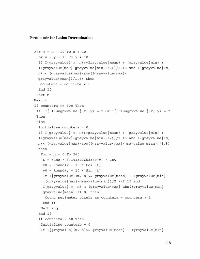
118
Pseudocode for Lesion Determination
For m = x - 10 To x + 10
For n = y - 10 To y + 10
If I{grayvalue}(m, n)>=Grayvalue{mean} + (grayvalue{min} +
((grayvalue{max}-grayvalue{min})/2))/2.15 and I{grayvalue}(m,
n) < (grayvalue{max}-abs((grayvalue{max}-
grayvalue{mean})/1.8) then
countera = countera + 1
End If
Next n
Next m
If countera >= 300 Then
If I{ llungbwvalue }(x, y) = 2 Or I{ rlungbwvalue }(x, y) = 2
Then
Else
Initialise countera = 0
If I{grayvalue}(m, n)>=grayvalue{mean} + (grayvalue{min} +
((grayvalue{max}-grayvalue{min})/2))/2.15 and I{grayvalue}(m,
n)< (grayvalue{max}-abs((grayvalue{max}-grayvalue{mean})/1.8)
then
For ang = 0 To 360
t = (ang * 3.14159265358979) / 180
x0 = Round(x - 10 * Cos (t))
y0 = Round(y - 10 * Sin (t))
If I{grayvalue}(m, n)>= grayvalue{mean} + (grayvalue{min} +
((grayvalue{max}-grayvalue{min})/2))/2.15 and
I{grayvalue}(m, n) < (grayvalue{max}-abs((grayvalue{max}-
grayvalue{mean})/1.8) then
Count perimeter pixels as countera = countera + 1
End If
Next ang
End if
If countera > 60 Then
Initialise counterb = 0
If I{grayvalue}(m, n)>= grayvalue{mean} + (grayvalue{min} +

119
((grayvalue{max}- grayvalue{min})/2))/2.15 and
I{grayvalue}(m, n)< (grayvalue{max}-abs((grayvalue{max}-
grayvalue{mean})/1.8) then
Count pixels inside the circle area
counterb = counterb + 1
End if
End if
If counterb > 280 Then
Determine the shape of nodule
Count the number of nodules
nodulecounter = nodulecounter + 1
End If
End if
End if

120
Bibliography
Abe, H., MacMahon, H., Engelmann, R., Li, Q., Shiraishi, J., Katsuragawa, S., Aoyama,
M., Ishida, T., Ashizawa, K., Metz, CE. & Doi, K. (January-February 2003). Computer-
aided Diagnosis in Chest Radiography: Results of Large-Scale Observer Tests at the
1996–2001 RSNA Scientific Assemblies. RadioGraphics, Vol.23, No.1. pp.255-265
Al-kabir, Z.W., Le, K. & Sharma, D. (2005). MEDADVIS: A Medical Advisory System.
KES, Vol-2. pp. 789-795.
Alnuweiri, M. H. & Kumar, V.K.P. (February 1991). Fast Image Labeling Using Local
Operators on Mesh-Connected Computers. IEEE Transactions on Pattern Analysis and
Machine Intelligence, Vol.13, No. 2. pp.202-207
Armato III, G. S. (October 2002). Lung segmentation: Applications in chest radiology,
Austral- Asian Journal of Cancer, ISSN-0972 2556, Vol. 2, No.2. pp1.
Armato III, G. S. (2003). Lung segmentation: Applications in chest radiology. Austral-
Asian Journal of Cancer, Vol. 2. pp. 124–132
Armato III, G. S., Giger, L. M. & MacMahon, H. (1998). Automated lung segmentation
in digitized posteroanterior chest radiographs, Acad Radiol, Vol.5. pp. 245-255.
Astola, J., Koskinen, L. & Neuvo, Y. (1992). Statistical Properties of Discrete
Morphological Filters. In Edward R. Dougherty (Ed.). Mathematical Morphology in
Image Processing. Mercel Dekker.

121
Aylward, R. S. & Kim, J. (2004). Statistics of pattern recognition. In Terry S.Yoo (Ed.).
Insight into images, principles and practice for segmentation, registration and image
analysis. A K Peters.
Bartz, D., Mayer, D., Fischer, J., Ley, S., Rio, D. A., Thust, S., Heussel, P. C., Kauczor,
U. H. & Straber, W. (2003). Hybrid segmentation and exploration of the human lungs.
Proceedings of the 14th IEEE visualization Conference. pp-177-181.
Basic Imaging: Introduction to Chest X-ray. (2005). Retrieved 5 April 2005.
http://radiology.creighton.edu/cxray.htm
Baxes, A. G. (1994). Digital image processing: Principles and applications. Wiley.
Beucher, S. (1983). Extrema of Grey-Tone Functions and Mathematical Morphology.
Technical Report N-793, Ecole des Mines de Paris.
Beucher, S. (1991). The Watershed Transformation Applied to Image Segmentation.
1Oth Conf. on Signal and Image Processing in Microscopy and Microanalysis,
Cambridge, UK. pp. 299-314.
Beucher, S., Bilodeau, M. & Yu, X. (1990). Road Segmentation by Watersheds
Algorithms. Proceedings of the Pro-art vision group PROMETHEUS workshop, Sophia-
Antipolis, France.
Beucher, S. & Lantuejoul, C. (1979). Use of Watersheds in contour detection.
International workshop on image processing: Real-time edge and Motion
detection/estimation, Rennes, France, pp.17-21.
Green, B. (2002). Edge Detection Tutorial. Retrieved 20 May, 2005.
http://www.pages.drexel.edu/~weg22/edge.html

122
Bratko, I. (2001). Prolog programming for artificial intelligence (3rd Ed.). Pearson.
Briggs, G. (2004). Pocket Guide to chest X-rays. McGraw Hill.
Brown, S. M., Wilson, S. L., Doust, D. B., Gill, W. R. & Sun, C. (1998). Knowledge-
based method for segmentation and analysis of lung boundaries in chest X-ray images.
Computerized Medical Imaging and Graphics, Vol. 22. pp 463-477
Burton, T. R., Isaacs, K. K., Fleming S. J. & Martonen, B.T. (2004). Computer
reconstruction of a human lung boundary model from magnetic resonance images.
Respiratory Care, Vol.49, No.2.
Campadelli, P., Casiraghi, E. & Columbano, S. (2004). Lung segmentation and nodule
Detection in postero-anterior chest radiographs. Retrieved 12 April, 2005.
http://homes.dsi.unimi.it/~campadel/Articoli/GIRPR2004.pdf.
Canny, J. (1986). A Computational Approach to Edge Detection. IEEE Transactions on
Pattern Analysis and Machine Intelligence, Vo. PAMI-8, No. 6. pp.679-687.
Cheng, D. & Goldberg, M. (1988). An algorithm for segmenting chest radiographs. SPIE
Visual Communications and Image Processing’88, Vol. 1001. pp. 261.
Columbia University Press. (2005). Retrieved 25 April, 2005.
http://www.answers.com/topic/X-ray
Corne, J., Carroll, M. & Delany, D. (2002). Chest X-ray made easy (2nd Ed.). Churchill
Livingstone.
Current status and future potential of computer-aided diagnosis in medical imaging
K Doi, PhD, British Journal of Radiology (2005) 78, 3-19.

123
Cypher, R.E., Sanz, J.L.C. & Snyder, L. (1990). Algorithms for image component
labelling on SIMD mesh-connected computers, IEEE Transactions on Computers,
Vol.39, No. 2, February 1990, pp-276-281.
Cypher, R.E., Sanz, J.L. C. & Snyder, L. (1989). An EREW PRAM Algorithm for image
component labeling. IEEE Transactions on Pattern Analysis and Machine Intelligence,
Vol 11, No.3. pp.258-262.
Derraz, F., Beladgham, M. & Khelif, M. (2004). Application of active contour models in
medical image segmentation. Proceedings of the International Conference on
information Technology: Coding and Computing, IEEE.
Dobrin, P. B., Viero, T. & Gabbouj, M. (1994). Fast Watershed algorithms: analysis and
extensions, SPIE Vol.2180, Nonlinear Image Processing V. pp. 209-220.
Doi K. (2005). Current status and future potential of computer-aided diagnosis in medical
imaging. British Journal of Radiology, Vol.78. pp.3-19.
Dougherty R. E. & Loce P. R. (1992). Efficient design strategies for the optimal binary
digital morphological filter: Probabilities, constraints, and structuring-element libraries.
In Edward R. Dougherty (Ed.). Mathematical Morphology in Image Processing. Mercel
Dekker.
Droogenbroeck V. M. (2005). Algorithms for Openings of Binary and Label Images with
Rectangular structuring Elements. Retrieved 10 July, 2005.
http://www.ulg.ac.be/telecom.
Duryea, J. & Boone M. J. (1995). A fully automated algorithm for the segmentation of
lung fields on digital chest radiographic images. Med Phys, Vol.22, No.2.

124
Flores, C. F. & Lotufo, de A. R. (2003). Object segmentation in image sequences by
Watershed from markers: A generic approach. Proceedings of the XVI Brazillian
Symposium on Computer Graphics and Image Processing. IEEE. pp.347
Foliguet, P. S., Vieira, B. M. & Araujo, De A. A. (2001). Segmentation into fuzzy
regions using topographic distance. IEEE Proceedings of the XIV Brazillian Symposium
on Computer Graphics and Image Processing, IEEE.
Fukunaga K. (1990). Introduction to statistical pattern recognition. (2nd ed.). Academic
Press.
Geometric Operations-Rotate. (2005). Retrieved 20 July, 2005.
http://homepages.inf.ed.ac.uk/rbf/HIPR2/rotate.htm
Giger, L. M. (1991). Automated scheme for lung nodule detection in chest radiographs.
Image Technology and Information Display, Vol. 23. pp. 1088-1091
Giger, L. M., Armato III, G. S., MacMahon, H. & Doi, K. (2000). Computerized
Detection of Lung Nodules. In Robin N. Strickland (Ed.). Image Processing Techniques
for Tumour Detection. Marcel Dekker. pp. 243-270.
Gil, J. & Kimmel, R. (2000). Efficient dilation, erosion, opening and closing algorithms.
In J. Goutsian, L. Vincent & D.S.Bloomberg (Eds.), Mathematical morphology and its
applications to image and signal Processing. Kluwer Academic Publishers.
Ginneken, V. B. & Loog, M. (2004). Pixel position regression – Application to Medical
Image Segmentation. 17th International Conference on Pattern Recognition (ICPR'04) –
Vol. 3.
Ginneken, V. B. & Romeny, H. B. M. T. (2000). Automatic segmentation of Lung fields
in chest radiographs. Med. Phys, Vol. 27 No.10. pp 2445-2455.

125
Ginneken, V. B., Romeny, H. B. M. T. & Viergever, A. M. (2001). Computer aided
diagnosis in chest radiography: A survey, IEEE Transactions on medical imaging, Vol.
20, No. 12.
Gregor, S. (2002). A theory in theories in information systems. Australian Journal of
Information systems, Special issue. pp.14-22.
Hara, T., Fujita, H., Lee, Y., Yoshimura, H. & Kido, S. (1999). Automated Lesion
Detection Methods for 2D and 3D Chest X-ray Images. Proceedings of the 10th
International Conference on Image. pp. 768-773.
Hara, T., Fujita, H. & Xu, J. (1997). Development of automated detection system for lung
nodules in chest radiograms. International Conference on Intelligent Information
Systems, IASTED. pp.71-74.
Hayashibe, R., Asano, N., Hirohata, H., Okumura, K., Kondo, S., Handa, S.,
Takizawa, M., Sone, S. & Oshita, S. (1996). An automatic lung cancer detection from
X-ray images obtained through yearly serial mass survey, Proceedings., International
Conference on Image Processing, 1996, Vol.1. pp.343-346.
Image Processing Toolbox. (2005). MATLAB (software tutorial).
Isa, M. N. A. & Sabarudin, S. (2005). Automatic detection of breast tumours from
ultrasound images using the modified seed based region growing technique. KES 2005,
LNAI 3682. pp.138-144.
Jain K. A. (1989). Fundamentals of digital image processing. Prentice Hall.
Kakeda, S., Moriya, J., Sato, H., Aoki, T., Watanabe, H., Oda, N., Katsuragawa, S.,
Yamamoto, K., Doi, K. & Roentgenol, J. A. (2004). Improved detection of lung nodules
on chest radiographs using a commercial computer-aided diagnosis system. AJR, Vol.182,
No.2. pp.505-510.

126
Kim, M. Y., Jaong, S. K. & Lee, H. M. (1989). A new algorithm for detection of Lung
Boundary. IEEE Engineering in Medicine and Biology Society, 11th Annual International
Conference.
Kling, R. (2005). Application Development with IDL: Combining analytical methods with
widget programming (Personally Published), www.rlkling.com, USA
Knowledge-based systems. (2005). Retrieved 2 December, 2005.
http://en.wikipedia.org/wiki/Knowledge-based_systems
Knowledge-based systems. (2005). Retrieved 4 December, 2005.
http://www.answers.com/topic/knowledge-based-system
Krupinski, A. E.(2000). Clinical Applications: Present and Future. In Robin N. Strickland
(Ed.). Image Processing Techniques for Tumor Detection. Marcel Dekker. pp. 47-70.
Kubota, Y., Mitsukura, Y., Fukumi, M., Akamatsu, N. & Yasutomo, M. (2005).
Automatic extraction system of a kidney region based on the Q-learning. KES 2005,
LNAI 3681. pp.1261-1267.
Kundel, L. H. & Dean, B. P. (2002). Tumor Imaging. In Robin N. Strickland (Ed.). Image
Processing Techniques for Tumor Detection. Marcel Dekker.
Kobayashi, T. (1996). Effect of a computer aided diagnosis scheme on Radiologists’
performance in detection of lung nodules on radiographs. Radiology, Vol.199. pp.843-
848.
Leymarie, F. & Levine, M.D. (1989). Curvature Morphology. Proc. Vision Interface '89.
pp. 102-109.

127
Lotufo, R. & Falcao, A.(2000). The ordered queue and the optimality of the watershed
approaches. In J. Goutsian, L. Vincent & D.S.Bloomberg (Eds.), Mathematical
morphology and its applications to image and signal Processing. Kluwer Academic
Publishers.
Matsumoto, T., Yoshimura, H., Doi, K., Giger, L. M., Kano, A., MacMahon, H., Abe, K.
& Montner, M. S. (1992). Image feature analysis of false positive diagnoses produced by
automated detection of lung nodules, Investigative Radiology, Vol. 27, No.8. pp.587-97.
Meijster, A., Roerdink, J.B.T.M., & Hesselink, W.H. (2000). A general algorithm for
computing distance transforms in linear time. In J. Goutsian, L. Vincent &
D.S.Bloomberg (Eds.), Mathematical morphology and its applications to image and
signal Processing. Kluwer Academic Publishers.
Meyer, F. (2000). Flooding and Segmentation. In J. Goutsian, L. Vincent &
D.S.Bloomberg (Eds.), Mathematical morphology and its applications to image and
signal Processing. Kluwer Academic Publishers.
Meyer, F. & Maragos, P. (1999). Multiscale Morphological Segmentations Based on
Watershed, Flooding and Eikonal PDE. Proceedings of the Second International
Conference on Scale-Space Theories in Computer Vision, LNCS Vol. 1682. pp.351 – 362.
Moga, N. A. & Gabbouj, M. (1997). Parallel Image Component Labeling with Watershed
Transformation. IEEE Transactions on Pattern analysis and Machine Intelligence. Vol 1.
No. 5. pp. 441-450.
Moga N. A. and Gabbouj, M. (1998) A Parallel Marker Based Image Segmentation with
Watershed Transformation. Journal of Parallel and Distributed Computing,
Vol. 51, No. 1. pp 27-45.
Moreira, R., Mendonca M. A., & Campilho, A. (2004). Detection of Rib Borders on X-
ray Chest Radiographs. ICIAR, LNCS 3212. pp.108-115.
128
Najman, L. & Schmitt, M. (1994). Watershed of a Continuous function. Signal
Processing, Elsevier Science, 38. pp.99-112.
Najman, L. & Schmitt, M. (1996). Geodesic saliency of watershed contours and
hierarchical segmentation. IEEE Transactions on Pattern Analysis and Machine
Intelligence, Vol. 18, No. 12, IEEE. pp.1163-1173.
Nakamori, N., Doi, K., Sabeti,V. & MacMahon, H. (1990). Image Feature Analysis and
computer aided diagnosis in digital radiolgraphy: Automated analysis of sizes of heart
and lung in chest images. Med. Phys, Vol.17, No.3.
Nguyen, T. H., Worring, M., & Boomgaard, van den R. (2003). Watersnakes: Enery
Driven Watershed Segmentation, IEEE Transactions on Pattern Analysis and Machine
Intelligence, Vol. 25, No. 3. pp. 330-342.
Nixon, M. & Aguado, A. (2002). Feature extraction & image processing. Newnes.
Park, M., Jin, S. J. & Wilson, S. L. (2001). Automatic extraction of lung boundaries by a
knowledge-based method. Visual Information Processing, Vol. 2. pp.14-19.
Park, M., Jin, S. J. & Wilson, S. L. (2002). Detection and measurement of hilar region in
chest radiograph. Visual Information Processing. pp.83-88.
Park, M., Jin, S. J. & Wilson, S. L. (2003). Detection and labelling ribs on expiration
chest radiographs. The Physics of Medical Imaging conference at SPIE, San Diego USA,
Vol. 4, No.21. pp.1021-1031.
Parker, J.R. (1996). Algorithm for Image processing and computer vision. (1st ed.).
Wiley.
129
Pietka, E. (1994). Lung segmentation in digital radiographs. Journal of Digital Imaging,
Vol 7, No 2. pp 79-84.
Preteux, F. (1992). On a Distance Function Approach for Gray-Level Mathematical
Morphology. In Edward R. Dougherty (Ed.). Mathematical Morphology in Image
Processing. Mercel Dekker.
Qian, Y. & Zhao, R. (1997). Image Segmentation Based on Combination of the Global
and Local Information. International Conference on Image Processing, IEEE, Vol.1.
pp.204-206.
Radiology: Chest Articles. (2005). Retrieved 5 April, 2005
http://www.emedicine.com/radio/CHEST.htm.
Rahman, M. M., Wan, T. & Desai, C. B. (2004). Medical image retrieval and registration:
Towards computer assisted diagnostic approach, IDEAS Workshop on Medical
Information Systems: The Digital Hospital. pp.78-89.
Rambabu, C., Rathore,T.S. & Chakrabarti, I. (2003). A New Watershed Algorithm
Based On Hillclimbing Technique for Image Segmentation, IEEE.
Rivest, J.F., Soille, P. & Beucher, S. (1993). Morphological Gradients. Journal of
Electronic Imaging. Vol. 02, No.04. pp.326-336.
Russel, S. & Norvig, P. (2003). Artificial intelligence: A modern approach. (2nd ed.).
Pearson Education.
Sacco, D. C., Lutzemberger, L. & Salvetti, O. (1997). Deformation Analysis of Three-
Dimensional Morphometric Structures. International Conference on Image Processing,
IEEE. pp.452.

130
Schalkoff , J. R. (1989). Digital image processing and computer vision. Wiley.
Scott, W. (2001). Lung Cancer: A guide to diagnosis and Treatment (1st Ed.). Addicus
Books.
Serra, J. (1982). Image analysis and Mathematical Morphology. Academic Press.1982
Sebestyen S. G. (1962). Decision-making processes in pattern recognition. Macmillan.
New York.
Senay, H. & Ignatius, E. (1994). A knowledge-based system for visualization Design.
IEEE Computer Graphics and Applications. pp.36-47.
Sivaramakrishna, R., Birbeck, S. J., Higgs, E. B., Cothren, M. R., Parisky, R. Y. &
Boswell, D. W. (Fall/Winter 2002). Computer aided detection of lung cancer from
Computed Tomography images, Technology Review Journal. pp-79-91.
Tveter R. D. (1998). The pattern recognition basis of artificial intelligence. IEEE.
Udupa, K. J. & Saha, K. P.(2004). Fuzzy connectedness. In Terry S.Yoo (Ed.). Insight
into images, principles and practice for segmentation, registration and image analysis. A
K Peters.
Vachier, C. and Meyer, F. (2005). The Viscous Watershed Transform. Journal of
Mathematical Imaging and Vision,Vol.22, No.2-3. pp. 251-267.
Vincent, L. (1992). Morphological Algorithms. In Edward R. Dougherty (Ed.).
Mathematical Morphology in Image Processing. Mercel Dekker.
Watman, C. and Le, K. (2003). Gravity Segmentation of Human Lungs from X-ray
images for sickness Classification. Fourth International Conference on Intelligent
Technologies (Intech'03). pp. 428-434.

131
Watman, C. & Le, K. (2004). Fuzzy analysis of X-ray images for automated disease
examination. KES 2004, LNAI 3214. pp.491-497.
Wechsler, H. & Sklansky, J. (1977). Finding the rib cage in chest radiographs. Pattern
Recognition, Pergamon Press 1977, Vol.9. pp. 21-30.
Wei, X. (1997). Development of an improved CAD scheme for automated detection of
lung nodules in digital chest images. Medical physics, Vol.24, No.9. pp.1395.
Wiemker, R. (2005). Aspects of computer aided detection (CAD) and volumetry of
pulmonary nodules using multislice CT. The British journal of radiology, 78. pp. S46-
S56.
Wilson S. S. (1992). Training structuring elements in morphological networks. Edward
R. Dougherty (Ed.). Mathematical Morphology in Image Processing. Mercel Dekker.
Winston H. P. (1992). Artificial intelligence. (3rd ed.). Pearson Education.
Wu, C. Y., Doi, K., Giger, L. M., Metz E. C. & Zhang W. (1994). Reduction of false
positives in computerized detection of lung nodules in chest radiographs using artificial
neural network, discriminant analysis, and rule based scheme. Journal of Digital
Imaging, Vol.7, No.4. pp.196-207
Xu, W. X. & Doi, K. (1995). Image feature analysis for computer-aided diagnosis:
Accurate determination of ribcage boundary in chest Radiographs. Med. Phys, Vol.22,
No.5.
Xu, W. X. & Doi, K. (1996). Image feature analysis for computer aided diagnosis:
Detection of right and left hemidiaphragm edges and delineation of lung field in chest
radiographs. Med. Phys, Vol. 23,No. 9. pp.1613-24.
132
Yin, K.R.(1994). Case Study Research: Design and Methods (2nd ed.). Applied Social
Research Methods Series, Vol.5. Sage.
Yoo, S. T. (July 2004). Segmentation basics, In Terry S.Yoo (Ed.). Insight into images,
principles and practice for segmentation, registration and image analysis. A K Peters.
Young Y. T. & Calvert W. T. (1974). Classification, estimation and pattern recognition.
Elsevier.
Zhou, H. Z. (2002). Lung cancer cell identification based on artificial neural network
ensembles. Artificial Intelligence in Medicine, vol.24, no.1. pp. 25-36.